06.1

Object Based Image Analysis: Introduction to eCognition

eCognition Developer 9.0

Description: We will be using eCognition and a simple image to introduce students to the concepts of Object Based Image Analysis

06.2

Object Based Image Interpretation: Introduction to eCognition

Objective: Use a synthesized image to demonstrate some of the concepts of object based

image analysis and contrast it to pixel based classifiers such as ERDAS Imagine. As part of this demonstration we will examine rule sets, the programming functionality of eCognition. You will start from a skeleton rule set and classify the St. Paul Campus data “stack”.

Background:

eCognition is an object based image analysis program. What we have worked with up to now in ERDAS Imagine is pixel based classification. In this lab we will see how eCognition segments the entire scene into image objects based on their spectral similarity. Then using elements of image interpretation such as size context to more effectively classify these objects

Your Mission Today:

Using the prepared content in the eCognition lab on the G drive, we will examine some introductory capability of eCognition and object based image interpretation. After you are familiar with the software you will create a rule set to classify the St. Paul Campus area of interest we used in the previous labs

Getting Set Up:

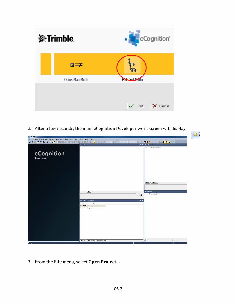
1. Open eCognition Developer 64 9.0 from the start menu. Within the All Programs listing, it is located in in the Trimble folder. When the following screen appears click on the Rule Set Mode icon

06.3

2. After a few seconds, the main eCognition Developer work screen will display

3. From the File menu, select Open Project…

06.4

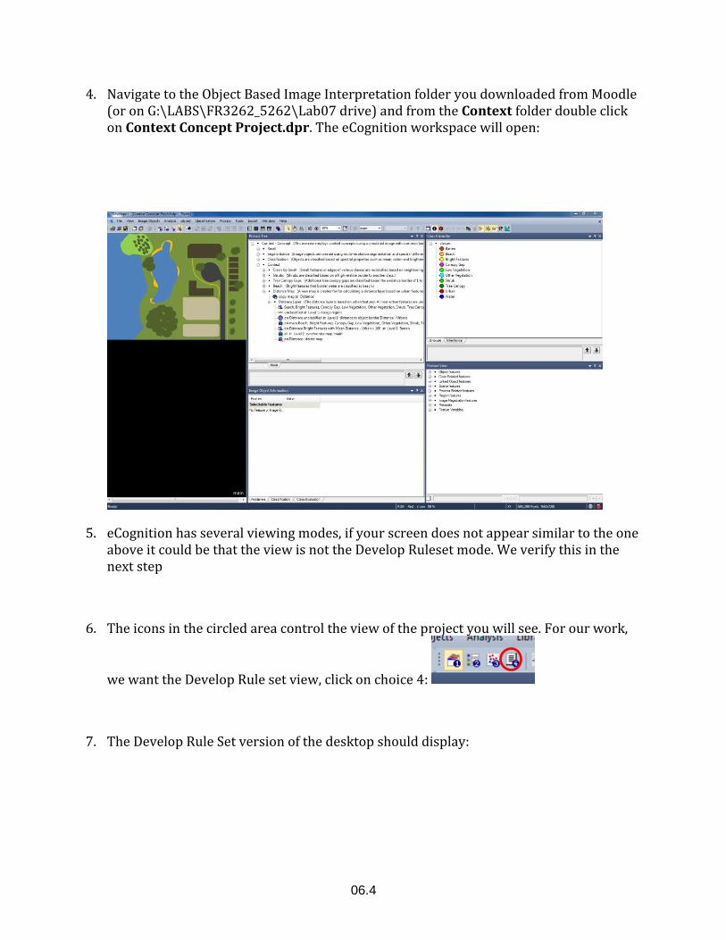
4. Navigate to the Object Based Image Interpretation folder you downloaded from Moodle (or on G:\LABS\FR3262_5262\Lab07 drive) and from the Context folder double click on Context Concept Project.dpr. The eCognition workspace will open:

5. eCognition has several viewing modes, if your screen does not appear similar to the one above it could be that the view is not the Develop Ruleset mode. We verify this in the next step

6. The icons in the circled area control the view of the project you will see. For our work,

we want the Develop Rule set view, click on choice 4:

7. The Develop Rule Set version of the desktop should display:

06.5

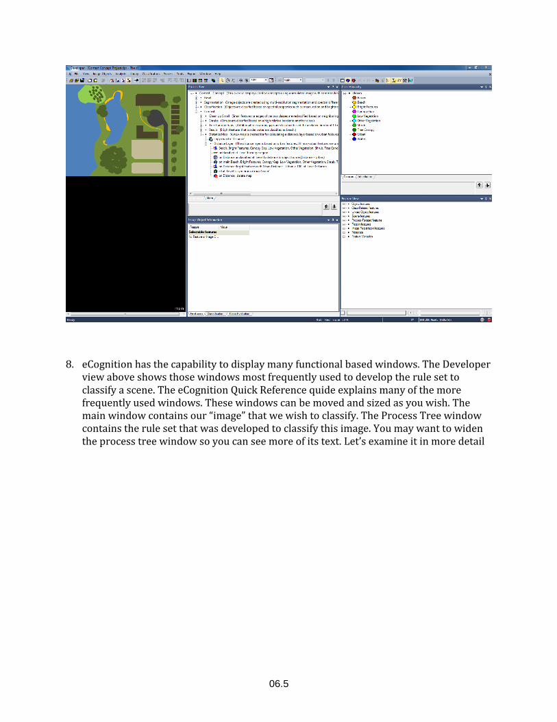
8. eCognition has the capability to display many functional based windows. The Developer view above shows those windows most frequently used to develop the rule set to classify a scene. The eCognition Quick Reference quide explains many of the more frequently used windows. These windows can be moved and sized as you wish. The main window contains our “image” that we wish to classify. The Process Tree window contains the rule set that was developed to classify this image. You may want to widen the process tree window so you can see more of its text. Let’s examine it in more detail

06.6

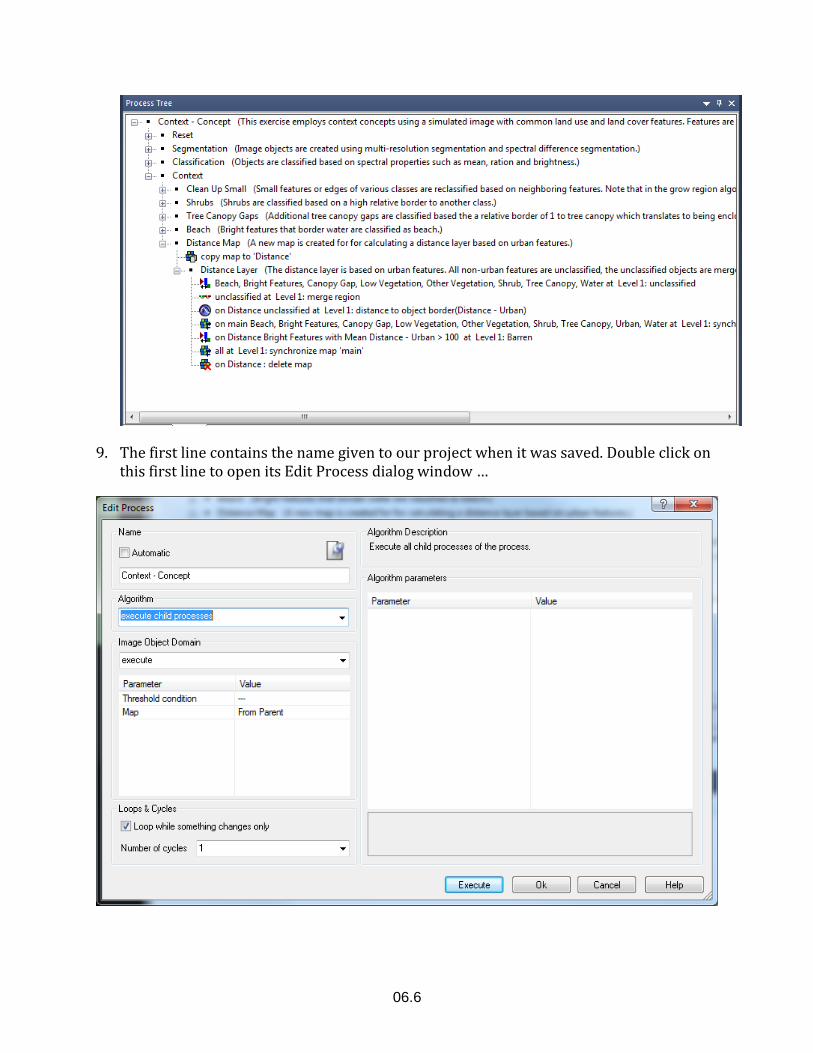
9. The first line contains the name given to our project when it was saved. Double click on this first line to open its Edit Process dialog window …

06.7

10. The Edit Process dialog appears for this line. The name is Context – Concept and the Algorithm that this step will perform is to ‘execute child processes’, that is executing this line will run all of the steps in the hierarchy below it. We want to execute the lines one by one so let’s Cancel from this dialog.

11. You can see that the next step, is called Reset and it has a plus indicating it is a grouping. Rule sets often are developed in this way, since major functional steps in the classification process may in fact take several individual eCognition commands to implement.This command clears out and prvious classification we may have done and starts us from a fresh position.

12. Go ahead and run the Reset section by right clicking on it and choosing Execute from the menu. (You could also double click on Reset and click on the Execute button in the Edit Process dialog box.

13. Notice that a time has been added… . This shows us that the step took less than a millisecond to execute

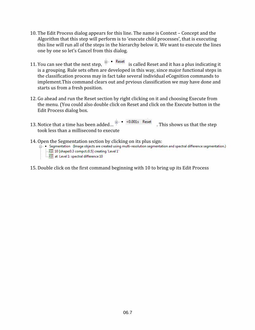
14. Open the Segmentation section by clicking on its plus sign:

15. Double click on the first command beginning with 10 to bring up its Edit Process

06.8

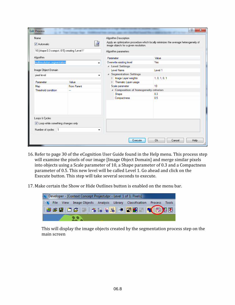
16. Refer to page 30 of the eCognition User Guide found in the Help menu. This process step will examine the pixels of our image [Image Object Domain] and merge similar pixels into objects using a Scale parameter of 10, a Shape parameter of 0.3 and a Compactness parameter of 0.5. This new level will be called Level 1. Go ahead and click on the Execute button. This step will take several seconds to execute.

17. Make certain the Show or Hide Outlines button is enabled on the menu bar.

This will display the image objects created by the segmentation process step on the main screen

06.9

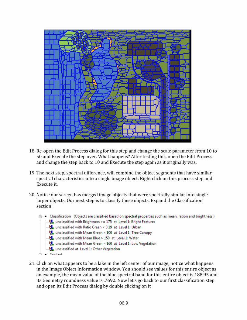
18. Re-open the Edit Process dialog for this step and change the scale parameter from 10 to 50 and Execute the step over. What happens? After testing this, open the Edit Process and change the step back to 10 and Execute the step again as it originally was.

19. The next step, spectral difference, will combine the object segments that have similar spectral characteristics into a single image object. Right click on this process step and Execute it.

20. Notice our screen has merged image objects that were spectrally similar into single larger objects. Our next step is to classify these objects. Expand the Classification section:

21. Click on what appears to be a lake in the left center of our image, notice what happens in the Image Object Information window. You should see values for this entire object as an example, the mean value of the blue spectral band for this entire object is 188.95 and its Geometry roundness value is .7692. Now let’s go back to our first classification step and open its Edit Process dialog by double clicking on it

06.10

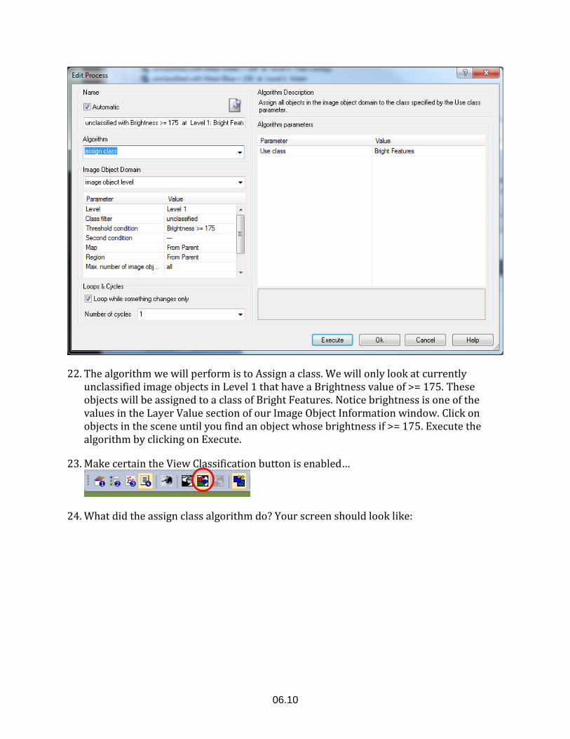
22. The algorithm we will perform is to Assign a class. We will only look at currently unclassified image objects in Level 1 that have a Brightness value of >= 175. These objects will be assigned to a class of Bright Features. Notice brightness is one of the values in the Layer Value section of our Image Object Information window. Click on objects in the scene until you find an object whose brightness if >= 175. Execute the algorithm by clicking on Execute.

23. Make certain the View Classification button is enabled…

24. What did the assign class algorithm do? Your screen should look like:

06.11

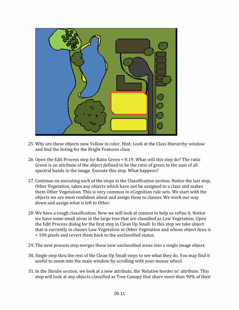
25. Why are these objects now Yellow in color. Hint: Look at the Class Hierarchy window and find the listing for the Bright Features class

26. Open the Edit Process step for Ratio Green < 0.19. What will this step do? The ratio Green is an attribute of the object defined to be the ratio of green to the sum of all spectral bands in the image. Execute this step. What happens?

27. Continue on executing each of the steps in the Classification section. Notice the last step, Other Vegetation, takes any objects which have not be assigned to a class and makes them Other Vegetation. This is very common in eCognition rule sets. We start with the objects we are most confident about and assign them to classes. We work our way down and assign what is left to Other.

28. We have a rough classification. Now we will look at context to help us refine it. Notice we have some small areas in the large tree that are classified as Low Vegetation. Open the Edit Process dialog for the first step in Clean Up Small. In this step we take object that is currently in classes Low Vegetation or Other Vegetation and whose object Area is < 100 pixels and revert them back to the unclassified status.

29. The next process step merges these now unclassified areas into a single image object.

30. Single step thru the rest of the Clean Up Small steps to see what they do. You may find it useful to zoom into the main window by scrolling with your mouse wheel.

31. In the Shrubs section, we look at a new attribute, the ‘Relative border to’ attribute. This step will look at any objects classified as Tree Canopy that share more than 90% of their

06.12

border with Other Vegetation and reclassify them as Shrub. Prior to running this step, zoom in to the area with the Other vegetation.

32. The Tree Canopy Gaps section looks at additional objects in the tree and classifies them as Canopy Gaps

33. What does the process step in Beach do? What element of image interpretation is this utilizing? Could you do this with a pixel based classifier like ERDAS Imagine’s unsupervised classifier?

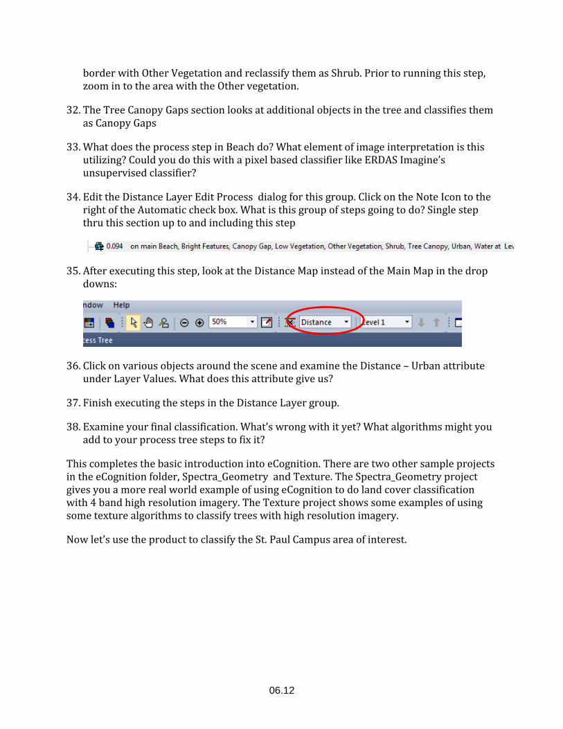
34. Edit the Distance Layer Edit Process dialog for this group. Click on the Note Icon to the right of the Automatic check box. What is this group of steps going to do? Single step thru this section up to and including this step

35. After executing this step, look at the Distance Map instead of the Main Map in the drop downs:

36. Click on various objects around the scene and examine the Distance – Urban attribute under Layer Values. What does this attribute give us?

37. Finish executing the steps in the Distance Layer group.

38. Examine your final classification. What’s wrong with it yet? What algorithms might you add to your process tree steps to fix it?

This completes the basic introduction into eCognition. There are two other sample projects in the eCognition folder, Spectra_Geometry and Texture. The Spectra_Geometry project gives you a more real world example of using eCognition to do land cover classification with 4 band high resolution imagery. The Texture project shows some examples of using some texture algorithms to classify trees with high resolution imagery.

Now let’s use the product to classify the St. Paul Campus area of interest.

06.13

Classify St. Paul Campus Area of Interest

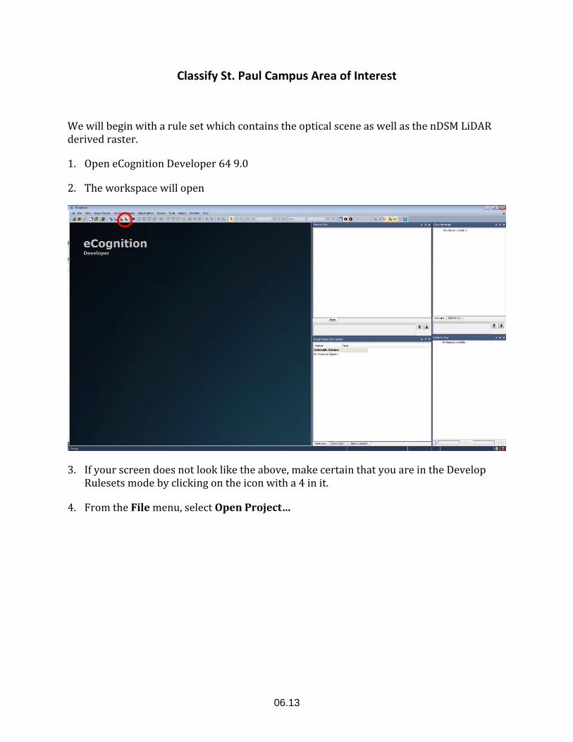
We will begin with a rule set which contains the optical scene as well as the nDSM LiDAR derived raster.

1. Open eCognition Developer 64 9.0

2. The workspace will open

3. If your screen does not look like the above, make certain that you are in the Develop Rulesets mode by clicking on the icon with a 4 in it.

4. From the File menu, select Open Project…

06.14

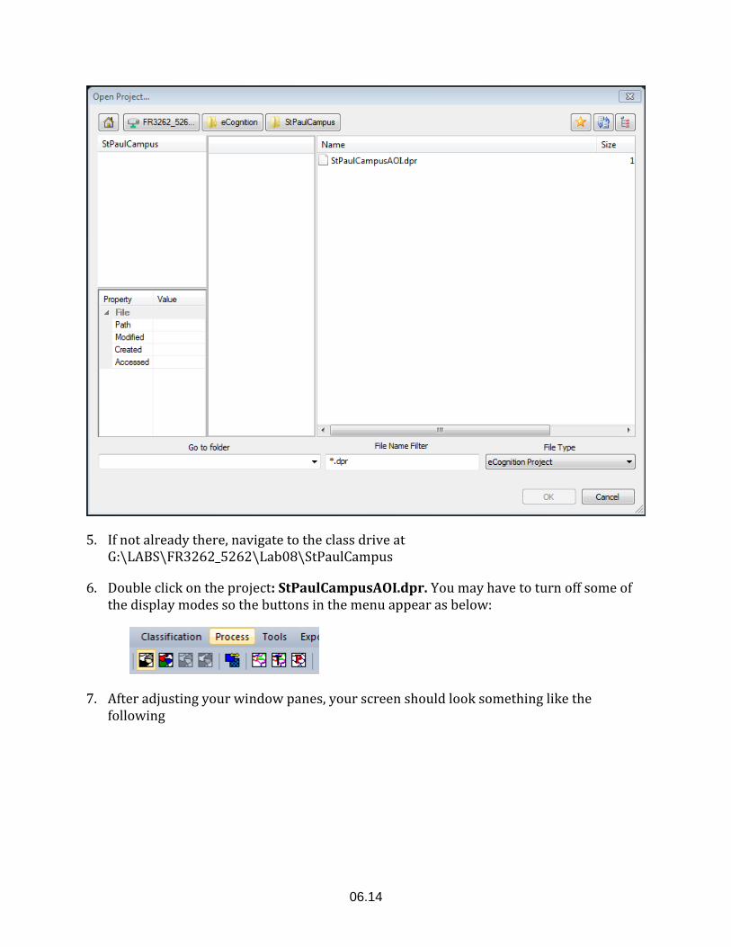
5. If not already there, navigate to the class drive at G:\LABS\FR3262_5262\Lab08\StPaulCampus

6. Double click on the project: StPaulCampusAOI.dpr. You may have to turn off some of the display modes so the buttons in the menu appear as below:

7. After adjusting your window panes, your screen should look something like the following

06.15

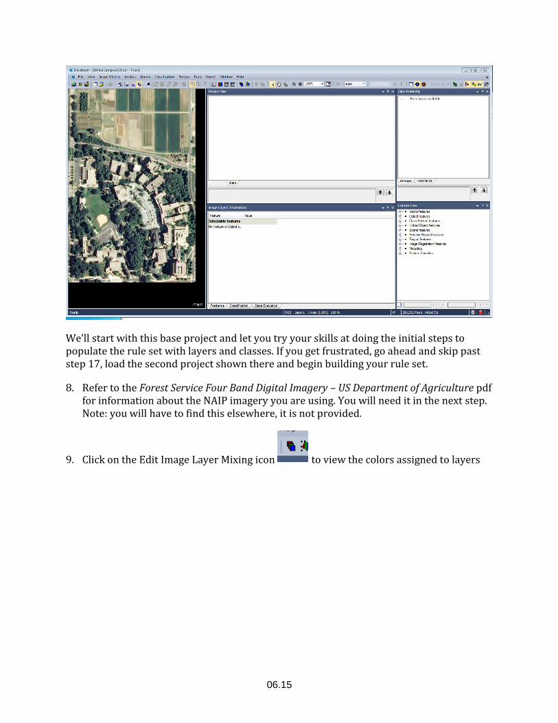
We’ll start with this base project and let you try your skills at doing the initial steps to populate the rule set with layers and classes. If you get frustrated, go ahead and skip past step 17, load the second project shown there and begin building your rule set.

8. Refer to the Forest Service Four Band Digital Imagery – US Department of Agriculture pdf for information about the NAIP imagery you are using. You will need it in the next step. Note: you will have to find this elsewhere, it is not provided.

9. Click on the Edit Image Layer Mixing icon to view the colors assigned to layers

06.16

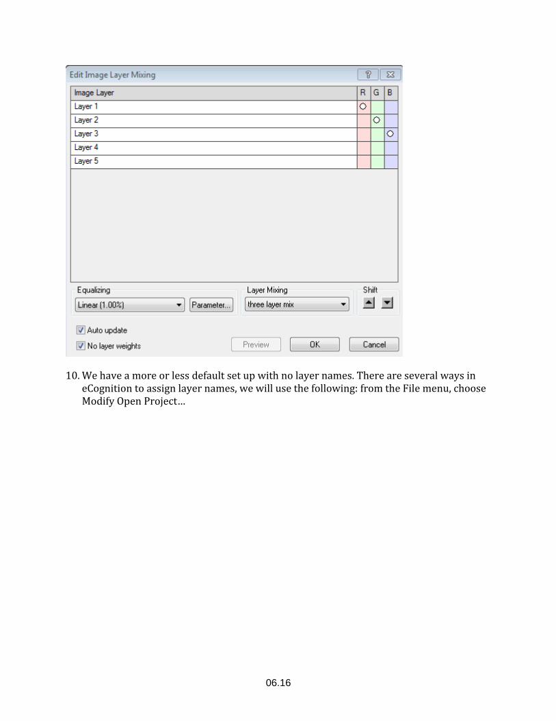
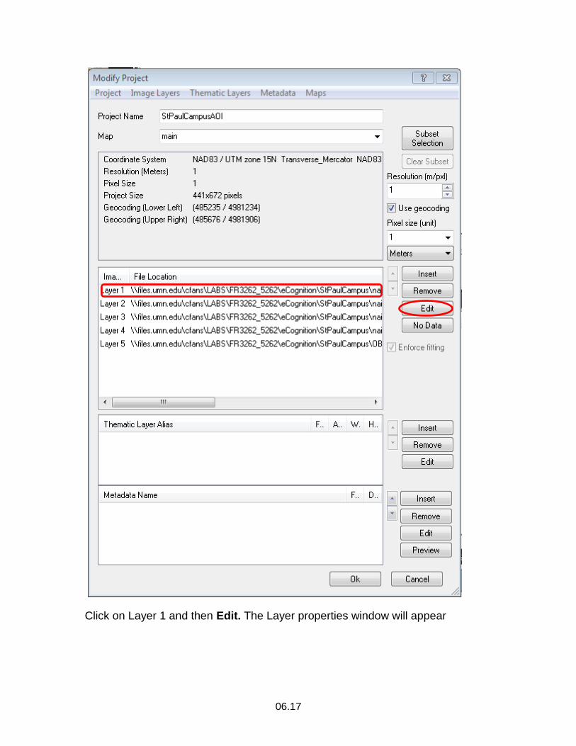
10. We have a more or less default set up with no layer names. There are several ways in eCognition to assign layer names, we will use the following: from the File menu, choose Modify Open Project…

06.17

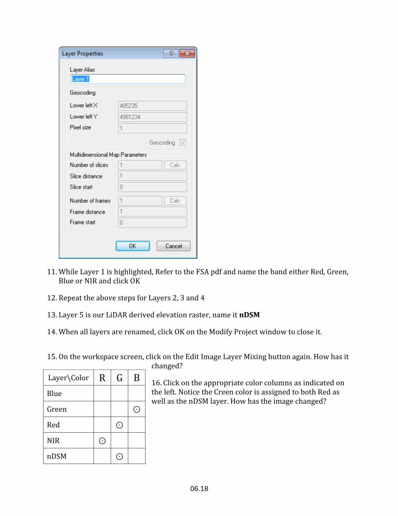
Click on Layer 1 and then Edit. The Layer properties window will appear

06.18

11. While Layer 1 is highlighted, Refer to the FSA pdf and name the band either Red, Green, Blue or NIR and click OK

12. Repeat the above steps for Layers 2, 3 and 4

13. Layer 5 is our LiDAR derived elevation raster, name it nDSM

14. When all layers are renamed, click OK on the Modify Project window to close it.

15. On the workspace screen, click on the Edit Image Layer Mixing button again. How has it changed?

16. Click on the appropriate color columns as indicated on the left. Notice the Creen color is assigned to both Red as well as the nDSM layer. How has the image changed?

Layer\Color R G B

Blue

Green ⊙

Red ⊙

NIR ⊙

nDSM ⊙

06.19

Your screen is now ready to begin developing a rule set to classify the scene. First we need to set up our classes. Our goal is to classify the image into the following:

Tree Canopy Grass Bushes & Low Vegetation Buildings Streets/Parking lots Sidewalks Bare Soil

17. Right click in the Class Hierarchy window and Insert a class for each of the above. Choose what every color you feel is reasonable

18. We will also need some temporary classes. Enter a class for _Tall, _Low and _Temp

Refer to your other rule sets and begin developing a rule set to classify this image. We have started you off by first creating an NDVI layer.

Go ahead and struggle a bit on your own to get the rule set started. If you get frustrated, look at the StPaulCampusAOI_B project as a good starting point upon which to build your rule set.

A completed rule set is also available for review (StPaulCampusAOI_Finished). This rule set took about 2 hours for a somewhat experienced TA to generate. More improvements could certainly be made to it but it should give you an idea of some of the capabilities of the product.

06.20

Lesson 06 Outcomes

At this point you should be able:

1. Understand how rule sets work in eCognition software

2. Be able to explain the difference between the capabilities of a pixel based classifier vs. an object based classifier.

3. Be familiar with some of the more common algorithms used in eCognition software.