Oblique Inlet Pressure Loss for Swirling Flow

Entering a Catalyst Substrate

T. Persoons ∗, M. Vanierschot and E. Van den Bulck

Katholieke Universiteit Leuven, Department of Mechanical Engineering,Celestijnenlaan 300A, B-3001 Leuven, Belgium, tel: +32-16-322511,

fax: +32-16-322985

Abstract

This experimental study investigates the oblique inlet pressure loss for the entry ofan annular swirling flow into an automotive catalyst substrate. The results are appli-cable to a wide range of compact heat exchangers. For zero swirl, the total pressureloss agrees with established expressions for pressure loss in developing laminar flowin parallel channels with finite wall thickness. For positive swirl, the additional pres-sure loss due to oblique flow entry is correlated to the tangential velocity upstreamof the catalyst, measured using laser Doppler anemometry. The obtained obliqueinlet pressure loss correlation can improve the accuracy of numerical calculations ofthe flow distribution in catalysts.

Key words: swirling, oblique, inclined flow, catalyst, heat exchanger, pressure loss,laser-Doppler anemometryPACS: 44.15.+a, 47.32.Ef, 47.80.Cb

Nomenclature

D, d hydraulic diameter of annular duct and substrate channel, mK pressure loss, relative to the substrate channel dynamic headL catalyst substrate length, mp pressure, PaR outer radius of the annular duct, mRe Reynolds number, based on d

∗ Corresponding author. Present address: Trinity College Dublin, Department ofMechanical Engineering, Parsons Building, Dublin 2, Ireland

Email address: tim.persoons@tcd.ie (T. Persoons).

Preprint submitted to Exp. Therm. Fluid Sci. 3 March 2008

S, SW swirl number and swirl vane settingU , V , W axial, radial and tangential velocity, m/su, v, w axial, radial and tangential turbulent fluctuation, m/sx, r axial and radial coordinate, mGreek symbolsα incidence angle of the oblique flow (tan α = Ut/U ), ◦

β LDA alignment angle, ◦

ε open frontal area ratioφ LDA beam intersection half-angle, ◦

θ tangential coordinate, ◦

ρ density, kg/m3

Subscriptsc substrate channeli inner radius of the annular ductm cross-sectional average

t transverse velocity component (e.g. Ut =√

V 2 + W 2)w hot-wire sensing element

1 Introduction1

Devices for exchange of mass or heat (e.g. catalytic converter, heat exchanger,2

particulate filters) operate optimally when the flow distribution over the cross-3

section is uniform. In this case, the pressure loss is minimal and the efficiency4

of mass or heat exchange is maximal. Particularly for a catalyst, local degra-5

dation or ageing [1] can be avoided by means of a uniform flow distribution.6

The degree of flow uniformity is mainly determined by the upstream flow con-7

figuration. Generally, a diffuser distributes the flow, and allows for a device8

with a larger cross-section than the connecting ducts. This approach increases9

the residence time within the exchange device, thereby increasing the overall10

exchange rate.11

For the case of automotive catalysts, a number of experimental studies [2,12

3, 4] investigate the influence of stationary and pulsating flow conditions and13

diffuser geometry on the catalyst flow uniformity. However, industrial design of14

inlet ducts and headers relies mainly on computational fluid dynamics (CFD).15

As shown in Fig. 1, a catalyst substrate consists of a large number of small16

parallel channels. As such, a porous volume approach is used to model such17

systems in CFD. The lengthwise flow resistance is determined based on the18

local axial velocity U immediately upstream of the porous volume, and the19

known pressure loss expressions. The overall pressure loss comprises (i) wall20

friction in fully developed flow, (ii) the momentum loss due to the boundary21

layer development, (iii) contraction and expansion losses at the inlet and outlet22

2

faces.23

The upstream flow configuration (particularly the diffuser) causes transverse24

velocity components Ut. Upon entering the channels, the oblique flow is straight-25

ened (see Fig. 1). Depending on the flow conditions, this process encompasses26

an additional pressure loss, here denoted ‘oblique inlet pressure loss’.27

Haimad [5] and Benjamin et al. [6, 7] have proven the importance of incor-28

porating the oblique inlet pressure loss in modeling the porous volume. Upon29

incorporating the oblique inlet pressure loss, CFD yields a flow distribution30

that agrees much better with the experimental results.31

Kuchemann and Weber [8] discuss the pressure loss for oblique flow in finned32

heat exchangers. For a heat exchanger with tubes resembling two-dimensional33

flat plates, the authors propose two models for the oblique inlet pressure loss34

coefficient Kα. The simplest model assumes that no suction can be sustained35

on the backside of the tubes, causing complete flow separation after the leading36

edge of the tubes. This condition is depicted schematically in Fig. 1 and yields37

a pressure loss K(1)α = tan2 α. This model is used by Benjamin et al. [6, 7].38

Since tan2 α · ρU2/2 = ρU2t /2, the entire transverse dynamic head is lost, and39

equals the oblique inlet pressure loss.40

A second, less conservative model [8] assumes that no loss occurs up to a41

critical angle αcrit. The value of αcrit is such that the pressure rise due to42

the streamtube expansion upon entering the channel equals the overall pres-43

sure loss in the channel for axial inlet flow, represented by K0. Symbolically,44

cos αcrit = 1/√

1 + K0 and the pressure loss is defined as:45

K(2)α =

0 ; |α| 6 αcrit

tan2 α−K0 ; |α| > αcrit

(1)

46

Kuchemann and Weber [8] provide some experimental data that confirm the47

proposed models. For laminar flow (inside the heat exchanger), the first model48

best agrees with the experiments. For turbulent flow, stronger suction can be49

sustained, and the inlet pressure loss is better predicted by the second model50

(Eq. (1)).51

Haimad [5] performed CFD calculations of oblique flow entering an automotive52

catalyst, not using a porous volume yet with full discretization of the substrate53

channels. The CFD results yield a correlation for the oblique inlet pressure54

loss of Kα = 0.831 tan2 α (R2 = 1.00). No experimental validation is provided.55

Meyer and Kroger [9] perform pressure drop measurements on several types56

of finned tube heat exchangers, for a broad range of angle of incidence α,57

3

between 0 and 80 ◦. The results collapse reasonably well to the first model of58

Kuchemann and Weber [8] (Kα = tan2 α), unlike the expression (1/sin θ − 1)259

suggested by Meyer and Kroger [9]. The experimental setup consists of a heat60

exchanger, placed at an incidence to the flow in a wind tunnel test section.61

In such a setup, the flow will deviate towards the part of the heat exchanger62

inclined away from the direction of flow. Therefore, the local angle of incidence63

can deviate significantly from the inclination angle of the heat exchanger.64

A number of studies [10, 11] examine the pressure drop and heat transfer of65

louvered fin heat exchangers. A higher louver angle α causes increased heat66

transfer, and a penalty in terms of pressure loss.67

Lee [10] discusses experimental results for the heat transfer coefficient and68

pressure drop in an array of inclined short plates, where the angle of attack69

α varies between 20 and 35 ◦ (350 < Re < 5000). Based on Fig. 18 [10], the70

contribution to the pressure loss due to the plate inclination behaves roughly71

as Kα = tan2 α, for Re between 700 and 2500, in spite of the very short plates72

(L/d ' 0.4). Lee [10] provides an interesting comparison of the heat transfer73

for a long flat plate and an array of inclined short plates with the same pressure74

loss, yielding an optimum angle α ' 30 ◦.75

DeJong and Jacobi [11] discuss experimental heat transfer and pressure drop76

results for a louvered-fin heat exchanger, with louver angles α between 18 and77

28 ◦. An increase in pressure drop may be noted for increasing louver angle,78

yet the range of α is too limited to assess the significance of the pressure loss79

results.80

Springer and Thole [12, 13] provide detailed velocity data for the entrance81

region of louvered-fin heat exchangers, yet no pressure loss data are provided.82

Wang and Tao [14] perform numerical calculations of laminar flow in an array83

of short inclined plates, as a function of the incidence angle α. The results84

show a strong relationship between the pressure drop and α. Upon reworking85

the data in Fig. 7 [14] for Re = 50, the contribution to the overall pressure loss86

due to the inclination varies as Kα = tan2 α, according to the simple model of87

Kuchemann and Weber [8].88

Yocum and O’Brien [15] performed wind tunnel experiments on inclined two-89

dimensional compressor blade cascades. The experimental pressure loss co-90

efficient in Fig. 18 [15] (for Re = 200 000) behaves according to the second91

model [8], with αcrit ' 15 ◦.92

Elvery and Bremhorst [16] provide experimental data for the pressure inside93

the tubes of a heat exchanger, placed at an incidence to the flow. The results94

show that the size of the recirculation region near the entrance grows for95

increasing values of α, from 0.5d for α = 0 to about 2d for α = 60 ◦, while the96

4

maximum subpressure is roughly independent of α.97

This paper provides accurate pressure loss data for oblique inlet flow condi-98

tions. The research uses an axisymmetric setup instead of a two-dimensional99

configuration, to eliminate flow redistribution across the cross-section. Fur-100

thermore, the local velocity is measured as close as possible to the inlet face101

of the channels. Although the research uses an automotive catalyst, the find-102

ings are relevant to all devices exchanging heat or mass, that consist of small103

parallel channels, operating in low Re conditions.104

2 Experimental approach105

This section discusses the experimental setup, the instrumentation, and ex-106

plains how the oblique inlet pressure loss is determined.107

2.1 Annular swirling flow rig108

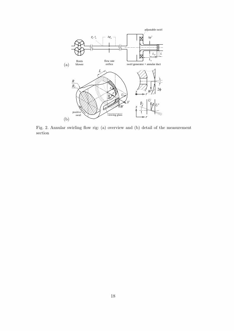
Figure 2a shows a schematic overview of the experimental setup. A Roots109

blower with ISO standardized flow rate orifice supplies air to a swirl generator,110

designed by the International Flame Research Foundation (IFRF) [17] for use111

on a 300 kW burner. The moveable block swirl generator allows to continuously112

adjust the swirl from zero to a maximum, corresponding to a ratio of tangential113

to axial velocity of about unity.114

The swirling flow is guided into a concentric annular duct by a smooth tran-115

sition. The annular duct features an outer and inner radius of R = 38.0 mm116

and Ri = 28.3 mm, corresponding to a hydraulic diameter D = 19.4 mm. The117

outer wall is PVC, the inner wall is aluminium, both with a smooth surface118

finish.119

Figure 2b shows a detail of the annular duct, which is connected to an auto-120

motive catalyst substrate of length L (400 cells per square inch, wall thickness121

4.3 × 10−3 inch, unwashcoated). The distance between substrate and swirl122

generator is 18D. Downstream of the catalyst, an outlet sleeve of length 2R123

is mounted. A cylindrical polar coordinate system [x, r, θ] is defined according124

to Fig. 2b.125

The catalyst substrate is mounted tight against the inner annulus wall, and126

sealed with silicon to prevent leakage. The test section and substrate are con-127

nected to the swirl generator by bolted flanges, taking care for proper align-128

ment. This allows to test various substrate lengths.129

5

2.2 Velocity measurements130

2.2.1 Laser-Doppler anemometry131

The axial and tangential velocity components U and W are measured inside132

the annular duct, in front of the catalyst substrate. A two-component laser-133

Doppler anemometer (LDA) is used with a 5 W Ar+ laser, with Bragg cell134

frequency shifting on both components. The system is operated in backscat-135

tering mode. Optical access is through a 1 mm thick glass microscope slide,136

flush with the outer annulus wall. As shown in Fig. 2b, the glass insert causes137

a minor defect, about 0.2 mm in height.138

To maximize the signal-to-noise ratio when measuring close to the inner annu-139

lus wall or the catalyst substrate, a second glass insert is mounted flush with140

in the inner annulus wall. Inside the annulus core, a beam dump reduces the141

amount of reflected laser light.142

The velocities are determined using a Dantec Flow Velocity AnalyzerTM with143

accompanying software, which is only used for data collection. Velocity weight-144

ing and statistics are performed using in-house software. An aerosol of DEHS145

oil is used as seeding, with particle diameters between 0.2 and 1 µm.146

The LDA system is carefully aligned and focused. The combination of a147

310 mm focal lens, a beam separation of 60 mm and a beam diameter of148

1.2 mm results in a measurement volume of ∅ 0.17 mm and 1.7 mm long.149

The beam intersection angle 2φ ' 11 ◦. While the LDA measurement vol-150

ume remains fixed in space, the swirl generator is traversed using a three-axis151

motorized translation stage, featuring a positioning accuracy within 50 µm.152

In each measurement point, sufficient samples are collected to reduce the mean153

axial velocity uncertainty to within 1%, based on a 95% confidence level. The154

inverse of the velocity magnitude is used as weighting factor, to reduce LDA155

velocity bias errors [18]. The mean axial velocity is verified using an ISO156

standardized flow rate orifice (see Fig. 2a), to within an uncertainty of ±5%.157

To measure the velocity close to the substrate inlet face, the LDA system is158

aligned at an angle β (> φ) to the annular duct (see Fig. 2b). As such, the LDA159

measures the velocity [U ′, W ′]. Assuming the radial velocity V is negligible,160

the actual velocity [U,W ] is obtained as W = W ′ and U = U ′/cosβ . A radial161

velocity measurement is feasible by applying different alignment angles β1162

and β2 in two measurements. These result in U ′1 = U cos β1 + V sin β1 and163

U ′2 = U cos β2 + V sin β2, from which the axial and radial velocity [U, V ] are164

readily obtained.165

For an incompressible fluid, the conservation of mass in a cylindrical polar166

6

coordinate system is expressed as:167

∂U

∂x+

1

r

∂ (rV )

∂r+

1

r

∂W

∂θ= 0 (2)

168

where ∂W/∂θ = 0 for axisymmetric flow (after careful annulus alignment, the169

deviation from axisymmetry is below 1 %). Equation (2) shows that the radial170

velocity V = 0 if ∂U/∂x = 0. The experiments reveal that ∂U/∂x 6= 0 close171

to the substrate, from a critical distance |x| < x0 (see Sect. 3.1). Beyond this172

critical distance (|x| > x0), ∂U/∂x ' 0, and therefore the radial velocity is173

negligible as well.174

The limited width of the annular duct R − Ri ' 0.25R limits the radial ve-175

locity magnitude. In fact, the annular geometry has been chosen after initial176

experiments with swirling flow in a circular duct. In swirling flow, the tangen-177

tial velocity W creates pressure gradients in the radial direction to balance178

the centrifugal forces:179

∂p

∂r=

ρW 2

r(3)

180

Initial experiments have been carried out using swirling flow in a circular duct,181

as opposed to the annular duct. In a circular duct, swirl causes a subpressure182

along the central axis. Since the tangential velocity decays in downstream183

direction, the central subpressure decreases, resulting in a positive pressure184

gradient ∂p/∂x along the duct axis. For strong swirl, ∂p/∂x becomes large185

enough to create backflow along the central axis, a phenomenon referred to186

as ‘vortex breakdown’ [19]. The presence of the catalyst substrate further187

increases ∂p/∂x , thereby promoting vortex breakdown. In these conditions,188

LDA measurements proved very difficult near the circular duct axis, due to189

seeding problems. The annular duct approach eliminates this problem.190

2.2.2 Hot-wire anemometry191

The axial velocity profile downstream of the catalyst has been measured using192

hot-wire anemometry. This measurement serves to verify the upstream axial193

velocity profile, as measured using LDA. To minimize the distortion of the194

downstream profile (due to the mixing of the laminar jets from the substrate195

channels) the velocity is measured only 1 mm from the outlet face, at x =196

L + 1 mm.197

Since the flow length scale is as small as d ' 1 mm, the sensor wire of standard198

hot-wire probes is too long (typically lw ' 1.5 mm). Therefore, a probe with199

shorter wire is custom-made for this purpose. As prescribed by Bruun [20],200

7

the wire length should be at least twice the cold wire length lw,cold to mini-201

mize conduction heat loss to the prongs. For a Tungsten sensor wire of 5 µm202

diameter, the cold length lw,cold ' 0.23 mm at U = 15 m/s [20]. As such, the203

probe wire is chosen lw = 0.5 mm long. The hot-wire is operated in constant204

temperature mode, with an overheat ratio of 1.8. The probe is calibrated in205

an open jet with an accuracy better than 1%.206

Due to the close measurement position, the velocity profile shows the individ-207

ual laminar jets. For each channel, the mean velocity is determined, resulting208

in a ‘discretized’ reference profile for the axial velocity (see Fig. 6).209

2.3 Evaluation of the oblique inlet pressure loss210

Static pressure taps are located at Lp = 9.6D upstream of the catalyst sub-211

strate (see Fig. 2a). The static pressure measured at that station ∆p∗ is cor-212

rected with the equivalent pressure drop ∆p(Lp) in an annular duct of length213

Lp, assuming fully developed turbulent flow (Re based on D varies between214

13 000 and 32 600), using the Colebrook-White correlation for smooth walls.215

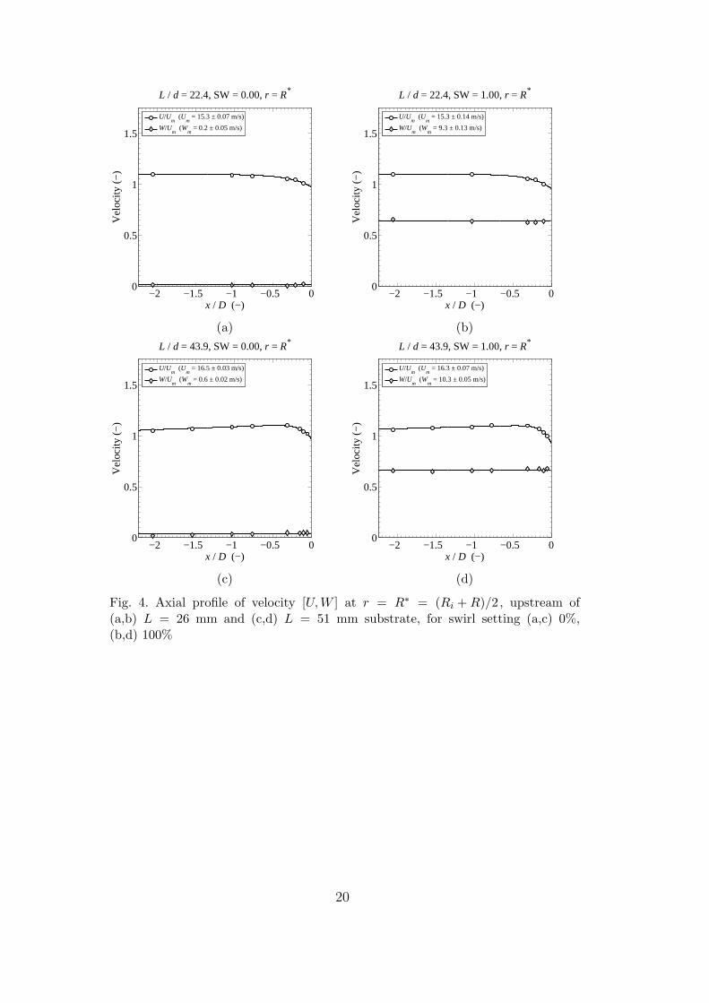
This yields the pressure loss ∆p (= ∆p∗ − ∆p(Lp)) over the substrate, with216

respect to the ambient pressure.217

∆p can be expressed as the sum of various sources of pressure loss, as described218

in App. A:219

∆p = (4fappL/d + Kcon + Kexp + Kα) ρU2c /2 (4)

220

where Uc is the mean velocity [m/s] inside the substrate channels. Uc = Um/ε ,221

where Um is the mean axial duct velocity [m/s] and ε is the substrate porosity.222

For zero swirl, the oblique inlet pressure loss vanishes (Kα = 0).223

From the substrate cell density and wall thickness, d and ε can be determined.224

For a 400/4.3 substrate, d ' 1.16 mm and ε ' 0.835. Each term in Eq. (4)225

depends on these values. Using the expressions for fapp, Kcon and Kexp in226

App. A, Eq. (4) is least-square fitted to the measured pressure loss, with the227

substrate wall thickness as fitting parameter. The hydraulic diameter d and228

porosity ε are determined as a function of the fixed cell density and the fitting229

parameter, i.e. the wall thickness.230

The fitting procedure results in a slightly different value for d and ε compared231

to the geometrical specifications. However, this approach is justifiable given the232

finite tolerances on the substrate geometry. After least-square fitting the wall233

thickness, Eq. (4) provides an excellent prediction of the measured pressure234

8

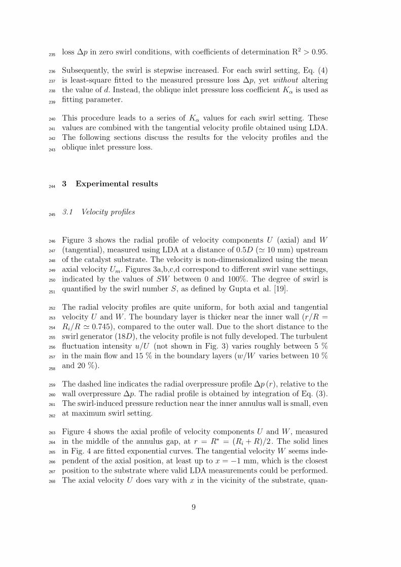
loss ∆p in zero swirl conditions, with coefficients of determination R2 > 0.95.235

Subsequently, the swirl is stepwise increased. For each swirl setting, Eq. (4)236

is least-square fitted to the measured pressure loss ∆p, yet without altering237

the value of d. Instead, the oblique inlet pressure loss coefficient Kα is used as238

fitting parameter.239

This procedure leads to a series of Kα values for each swirl setting. These240

values are combined with the tangential velocity profile obtained using LDA.241

The following sections discuss the results for the velocity profiles and the242

oblique inlet pressure loss.243

3 Experimental results244

3.1 Velocity profiles245

Figure 3 shows the radial profile of velocity components U (axial) and W246

(tangential), measured using LDA at a distance of 0.5D (' 10 mm) upstream247

of the catalyst substrate. The velocity is non-dimensionalized using the mean248

axial velocity Um. Figures 3a,b,c,d correspond to different swirl vane settings,249

indicated by the values of SW between 0 and 100%. The degree of swirl is250

quantified by the swirl number S, as defined by Gupta et al. [19].251

The radial velocity profiles are quite uniform, for both axial and tangential252

velocity U and W . The boundary layer is thicker near the inner wall (r/R =253

Ri/R ' 0.745), compared to the outer wall. Due to the short distance to the254

swirl generator (18D), the velocity profile is not fully developed. The turbulent255

fluctuation intensity u/U (not shown in Fig. 3) varies roughly between 5 %256

in the main flow and 15 % in the boundary layers (w/W varies between 10 %257

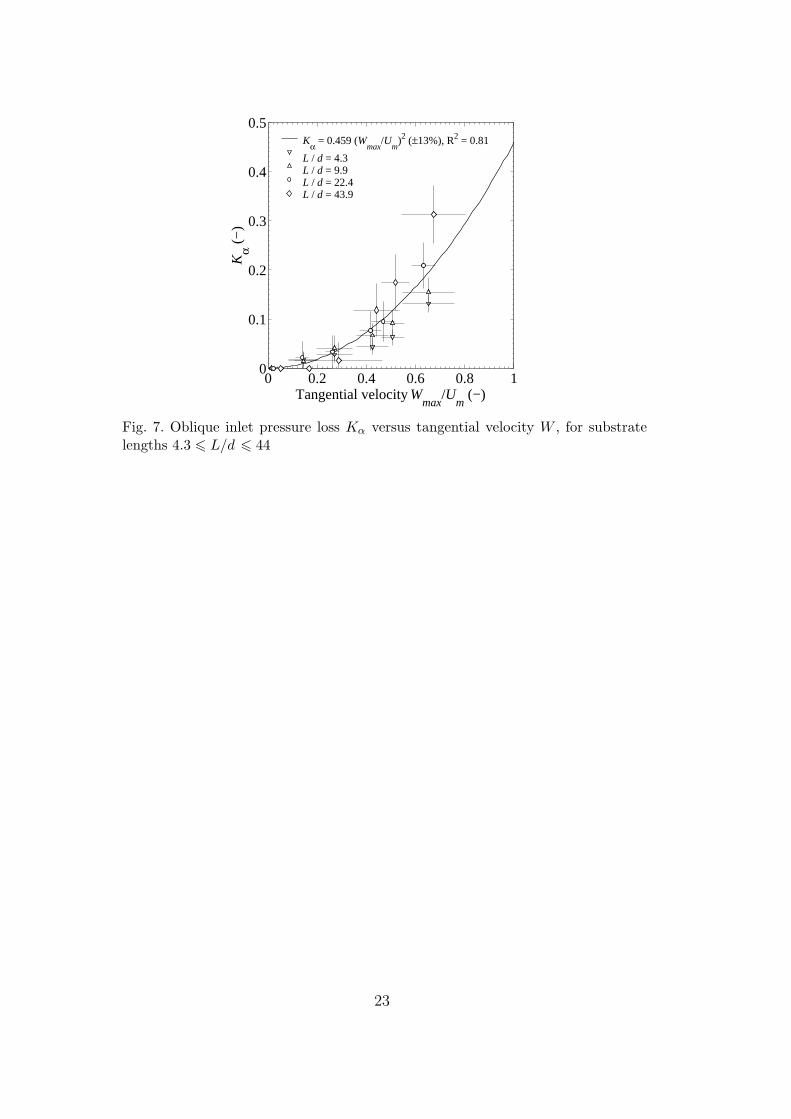
and 20 %).258

The dashed line indicates the radial overpressure profile ∆p (r), relative to the259

wall overpressure ∆p. The radial profile is obtained by integration of Eq. (3).260

The swirl-induced pressure reduction near the inner annulus wall is small, even261

at maximum swirl setting.262

Figure 4 shows the axial profile of velocity components U and W , measured263

in the middle of the annulus gap, at r = R∗ = (Ri + R)/2. The solid lines264

in Fig. 4 are fitted exponential curves. The tangential velocity W seems inde-265

pendent of the axial position, at least up to x = −1 mm, which is the closest266

position to the substrate where valid LDA measurements could be performed.267

The axial velocity U does vary with x in the vicinity of the substrate, quan-268

9

tified by a stagnation length x0. Close to the substrate, radial flow spreading269

occurs as indicated in Fig. 5.270

From the continuity equation (2) follows ∂ (rV )/∂r = −r ∂U/∂x , for axisym-271

metric flow. Thus, an order of magnitude analysis can be performed:272

∆U

x0

' 1

R

R Vmax

D/4⇒ Vmax

Um

' 1/4

x0/D

∆U

Um

(5)273

where the experimental results show that ∆U/Um ' 0.1. Based on the LDA274

results, x0/D varies between 0.1 and 0.5. As such, Vmax/Um is estimated to275

vary between 0.25 and 0.05. In terms of dynamic pressure, the radial compo-276

nent ρV 2/2 is therefore small (yet not negligible) compared to the tangential277

component ρW 2/2.278

The measurement of the full velocity vector [U, V,W ] within |x| < x0 proved279

too difficult using LDA, since reflections rapidly reduce the signal quality in280

the vicinity of the substrate. This has not been further pursued. Since W281

remains unchanged in x-direction, the tangential velocity profile is measured282

at x = −0.5D, where the LDA signal quality is adequate.283

In a follow-up paper [21], stereoscopic particle image velocimetry (PIV) is284

used in the same experimental setup to study the three-dimensional velocity285

field [U, V,W ] close to the substrate inlet face (|x| ' 0.2 mm). The relation286

between the stagnation length x0, flow uniformization and catalyst pressure287

drop K is discussed [21].288

Figure 6 shows the radial profile of axial velocity, measured using hot-wire289

anemometry (HWA), at 1 mm downstream of the catalyst substrate. The290

circular markers represent the actual velocity measurements, exhibiting the291

features of laminar jets issuing from the substrate channels. The solid staircase292

line represents the mean velocity for each individual channel, with vertical293

lines representing the 95% error margins. Due to the short substrate length294

(L/d = 22.4), the individual channel profiles are not fully developed.295

Upon comparison of Fig. 6a,b to Fig. 3a,d, there is some difference in the296

upstream (x = −0.5D) U profile and the solid line in Fig. 6a,b representing the297

channel-averaged downstream velocity (x = L+1 mm). Near the inlet face, the298

radial spreading causes a further uniformization of the axial velocity profile.299

This effect could not be adequately measured with LDA. Instead, stereoscopic300

PIV is used in a follow-up study [21] to investigate the flow stagnation region.301

10

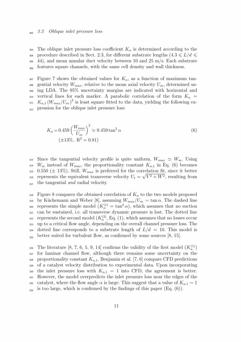
3.2 Oblique inlet pressure loss302

The oblique inlet pressure loss coefficient Kα is determined according to the303

procedure described in Sect. 2.3, for different substrate lengths (4.3 6 L/d 6304

44), and mean annular duct velocity between 10 and 25 m/s. Each substrate305

features square channels, with the same cell density and wall thickness.306

Figure 7 shows the obtained values for Kα, as a function of maximum tan-307

gential velocity Wmax, relative to the mean axial velocity Um, determined us-308

ing LDA. The 95% uncertainty margins are indicated with horizontal and309

vertical lines for each marker. A parabolic correlation of the form Kα =310

Kα,1 (Wmax/Um )2 is least square fitted to the data, yielding the following ex-311

pression for the oblique inlet pressure loss:312

Kα = 0.459(

Wmax

Um

)2

' 0.459 tan2 α (6)

(±13%, R2 = 0.81)

Since the tangential velocity profile is quite uniform, Wmax ' Wm. Using313

Wm instead of Wmax, the proportionality constant Kα,1 in Eq. (6) becomes314

0.550 (± 13%). Still, Wmax is preferred for the correlation fit, since it better315

represents the equivalent transverse velocity Ut =√

V 2 + W 2, resulting from316

the tangential and radial velocity.317

Figure 8 compares the obtained correlation of Kα to the two models proposed318

by Kuchemann and Weber [8], assuming Wmax/Um = tan α. The dashed line319

represents the simple model (K(1)α = tan2 α), which assumes that no suction320

can be sustained, i.e. all transverse dynamic pressure is lost. The dotted line321

represents the second model (K(2)α , Eq. (1), which assumes that no losses occur322

up to a critical flow angle, depending on the overall channel pressure loss. The323

dotted line corresponds to a substrate length of L/d = 10. This model is324

better suited for turbulent flow, as confirmed by some sources [8, 15].325

The literature [8, 7, 6, 5, 9, 14] confirms the validity of the first model (K(1)α )326

for laminar channel flow, although there remains some uncertainty on the327

proportionality constant Kα,1. Benjamin et al. [7, 6] compare CFD predictions328

of a catalyst velocity distribution to experimental data. Upon incorporating329

the inlet pressure loss with Kα,1 = 1 into CFD, the agreement is better.330

However, the model overpredicts the inlet pressure loss near the edges of the331

catalyst, where the flow angle α is large. This suggest that a value of Kα,1 = 1332

is too large, which is confirmed by the findings of this paper (Eq. (6)).333

11

4 Conclusions334

The oblique inlet pressure loss has been determined experimentally for an au-335

tomotive catalyst substrate, using an annular swirling flow rig. Laser-Doppler336

anemometry (LDA) is used to determine the upstream axial and tangential337

velocity profiles, as close as possible to the substrate inlet face.338

The axial velocity profile exhibits radial spreading close to the inlet face.339

However, the tangential velocity profile remains constant up to the closest340

measurable distance to the inlet face, |x| ' 1 mm. In the vicinity of the inlet341

face, LDA signal quality rapidly deteriorates due to wall reflections. Therefore,342

stereoscopic particle image velocimetry (PIV) is used in a follow-up paper [21]343

to examine the axial, tangential and radial velocity closer to the inlet face344

(|x| ' 0.2 mm).345

Four substrate lengths (4.3 6 L/d 6 44) are investigated, for six swirl settings346

(0 6 S 6 0.6) and three annular duct Reynolds numbers (13000 6 Re 6347

32600). Based on the substrate channel diameter, 850 6 Red 6 2100.348

For zero swirl, the substrate pressure loss is well predicted by the established349

expressions for pressure loss in developing laminar flow in channels with finite350

wall thickness, as summarized in App. A.351

For positive swirl, the additional pressure loss due to oblique flow entry is352

correlated to the peak tangential velocity upstream of the substrate. Although353

there is evidence of radial velocity near the inlet face, the tangential velocity354

is not significantly affected. As such, it is argued that the peak tangential355

velocity is most representative for the overall transverse dynamic pressure.356

Figure 7 confirms that the oblique inlet pressure loss coefficient Kα correlates357

satisfactorily to the squared ratio of tangential to axial velocity, or:358

Kα = 0.459(

Wmax

Um

)2

' 0.459 tan2 α

(±13%, R2 = 0.81)

This result agrees with the literature [8, 7, 6, 5, 9, 14]. The proportionality359

constant Kα,1 = 0.459 is smaller than unity, where the upper limit value of360

Kα,1 = 1 corresponds to a total loss of transverse dynamic pressure [8].361

For the case of automotive catalysts, the value of Kα,1 = 0.459 (± 13%) seems362

appropriate, based on the experience of Benjamin et al. [7, 6] in implementing363

the inlet pressure loss with Kα,1 = 1 in CFD.364

12

Acknowledgements365

The authors thank E. Delarue and K. De Vocht for the assistance during the366

initial measurement campaign on the circular duct swirling flow rig.367

A Pressure loss in channel flow368

The following sections review the different sources of pressure loss associated369

with flow through an array of parallel straight channels, particularly for lami-370

nar flow (Re < 2300). Each pressure loss contribution is non-dimensionalized371

using the dynamic head ρU2c /2, based on the mean channel velocity Uc.372

A.1 Fully developed flow373

For fully developed flow, the pressure loss is governed by wall friction, and374

quantified as 4fL/d . For laminar flow, the product of the Fanning friction375

factor f and Re is constant, e.g. f·Re ' 14.227 for square channels [22].376

A.2 Boundary layer development377

The velocity distribution at the channel inlet is assumed uniform, since the378

flow enters multiple parallel channels from a large cross-sectional area. The379

boundary layer development requires momentum transport from the wall to380

the channel center. Furthermore, the wall velocity gradient changes for a de-381

veloping profile, so the wall friction is larger in the developing flow region.382

Both effects combined cause an increase in pressure loss, quantified by Shah383

and London [22], Shah [23] as an apparent friction factor fapp (> f):384

fapp Re(x+

)=

3.44√x+

+f·Re + K∞

4x+ − 3.44√x+

1 + Cx+−2 (A.1)385

where x+ = (x/d)/Re . The effect of the boundary layer development can386

be singled out as Kdev (x+) = 4 (fapp Re (x+)− f·Re) x+. This incremental387

pressure loss tends to K∞ for x+ →∞. For a square cross-section, K∞ = 1.43388

and C = 0.000 29 [23], although other studies yield different values for K∞,389

e.g. K∞ = 1.55 [24].390

13

A.3 Contraction and expansion loss391

Upon entering and exiting channels with finite wall thickness, the flow respec-392

tively contracts and expands, according to the open area ratio ε. Kays and393

London [25], Kays [26] provide empirical data for the associated pressure loss394

in heat exchangers. For laminar flow in a square channel:395

Kcon = (1− Cc,0) (1− ε2) + 2(k

(in)d − 1

)Kexp = (1− ε)2 − 2

(k

(out)d − 1

)ε

(A.2)

where Cc,0 ' 0.615 [26] is the vena contracta area ratio for ε = 0 (i.e. entrance396

from an infinite reservoir). k(in)d and k

(out)d quantify the distribution of momen-397

tum, respectively at the channel inlet and outlet (kd =∫A (U/Um )2 dA/A >398

1). Lundgren et al. [24] explain how kd is related to Kdev from Sect. A.2. As-399

suming a fully developed outlet profile, k(out)d = 1.3785 [24], yielding Kexp =400

(1− ε)2 − 0.757 ε.401

Kays [26] evaluates k(in)d for a fully developed profile, thereby partially incor-402

porating the pressure loss due to the boundary layer development in Kcon. In403

the opinion of the authors, it is preferable to assume a uniform velocity profile404

near the inlet, immediately following the vena contracta. As such, k(in)d = 1 and405

Kcon = 0.385 (1− ε2). Thus, the contraction and expansion loss is considered406

separate from the boundary layer development loss.407

A.4 Overall408

The core of this paper concerns the additional pressure loss due to oblique flow409

inlet Kα. All pressure loss contributions (excluding temperature changes 1 ) are410

added to yield the overall pressure loss:411

K = 4fappL/d + Kcon + Kexp + Kα (A.3)412

1 For lengthwise temperature changes, the density and velocity change accordingly,causing an additional pressure loss or rise depending on ρ (x)/ρ (0) .

14

References413

[1] C.H. Bartholomew, Mechanisms of catalyst deactivation, Applied Catal-414

ysis A-General 212 (1-2) (2001) 17-60.415

[2] T. Persoons, A. Hoefnagels, E. Van den Bulck, Experimental validation416

of the addition principle for pulsating flow in close-coupled catalyst man-417

ifolds, Journal of Fluids Engineering-Transactions of the ASME 128 (4)418

(2006) 656-670.419

[3] T. Persoons, E. Van den Bulck, S. Fausto, Study of pulsating flow in420

close-coupled catalyst manifolds using phase-locked hot-wire anemome-421

try, Experiments in Fluids 36 (2) (2004) 217-232.422

[4] S.F. Benjamin, C.A. Roberts, J. Wollin, A study of pulsating flow in423

automotive catalyst systems, Experiments in Fluids 33 (5) (2002) 629-424

639.425

[5] N. Haimad, A theoretical and experimental investigation of the flow per-426

formance of automotive catalytic converters, PhD thesis, Coventry Uni-427

versity, UK, 1997.428

[6] S.F. Benjamin, H. Zhao, A. Arias-Garcia, Predicting the flow field inside429

a close-coupled catalyst: The effect of entrance losses, Proceedings of the430

IMechE C-Journal of Mechanical Engineering Science 217 (3) (2003) 283-431

288.432

[7] S.F. Benjamin, N. Haimad, C.A. Roberts, J. Wollin, Modelling the flow433

distribution through automotive catalytic converters. Proceedings of the434

IMechE C-Journal of Mechanical Engineering Science 215 (4) (2001) 379-435

383.436

[8] D. Kuchemann, J. Weber, Aerodynamics of Propulsion, McGraw-Hill,437

London, 1953, Chap. 12.438

[9] C.J. Meyer, D.G. Kroger, Air-cooled heat exchanger inlet flow losses,439

Applied Thermal Engineering 21 (7) (2001) 771-786.440

[10] Y.N. Lee, Heat-transfer and pressure-drop characteristics of an array of441

plates aligned at angles to the flow in a rectangular duct, International442

Journal of Heat and Mass Transfer 29 (10) (1986) 1553-1563.443

[11] N.C. DeJong, A.M. Jacobi, Localized flow and heat transfer interactions444

in louvered-fin arrays, International Journal of Heat and Mass Transfer445

46 (3) (2003) 443-455.446

[12] M.E. Springer, K.A. Thole, Experimental design for flowfield studies of447

louvered fins, Experimental Thermal and Fluid Science 18 (3) (1998) 258-448

269.449

[13] M.E. Springer, K.A. Thole, Entry region of louvered fin heat exchangers,450

Experimental Thermal and Fluid Science 19 (4) (1999) 223-232.451

[14] L.B. Wang, W.Q. Tao, Heat-transfer and fluid-flow characteristics of452

plate-array aligned at angles to the flow direction, International Jour-453

nal of Heat and Mass Transfer 38 (16) (1995) 3053-3063.454

[15] A.M. Yocum, W.F. O’Brien, Separated flow in a low-speed two-455

dimensional cascade: Part 2. Cascade performance, Journal of456

15

Turbomachinery-Transactions of the ASME 115 (3) (1993) 421-434.457

[16] D.G. Elvery, K. Bremhorst, Wall pressure and effective wall shear stresses458

in heat exchanger tube inlets with application to erosion corrosion, Jour-459

nal of Fluids Engineering-Transactions of the ASME 119 (4) (1997) 948-460

953.461

[17] W. Leuckel, Swirl intensities, swirl types and energy losses of different462

swirl generating devices, International Flame Research Foundation, Ij-463

muiden, The Netherlands, 1969, G02/a/16.464

[18] R.D. Gould, K.W. Loseke, A comparison of four velocity bias correction465

techniques in laser doppler velocimetry, Journal of Fluids Engineering-466

Transactions of the ASME 115 (3) (1993) 508-514.467

[19] A. Gupta, G. Lilley, N. Syred, Swirl Flows, Abacus Press, Tunbridge468

Wells, UK, 1984.469

[20] H.H. Bruun, Hot-Wire Anemometry: Principles and Signal Analysis, Ox-470

ford University Press, Oxford, UK, 1995, pp.21-26.471

[21] T. Persoons, M. Vanierschot, E. Van den Bulck, Stereoscopic PIV mea-472

surements of swirling flow entering a catalyst substrate, Experimental473

Thermal and Fluid Science (in review).474

[22] R.K. Shah, A.L. London, Laminar flow forced convection in ducts, in:475

R.F. Irvine, J.P. Hartnett, (Eds.), Advances in Heat Transfer, Academic476

Press, New York, 1978, pp.98-212.477

[23] R.K. Shah, A correlation for laminar hydrodynamic entry length solu-478

tions for circular and noncircular ducts, Journal of Fluids Engineering-479

Transactions of the ASME 100 (2) (1978) 177-179.480

[24] T.S. Lundgren, E.M. Sparrow, J.B. Starr, Pressure drop due to the481

entrance region in ducts of arbitrary cross section, Journal of Basic482

Engineering-Transactions of the ASME 86 (3) (1964) 620-626.483

[25] W.M. Kays, A.L. London, Compact Heat Exchangers, McGraw-Hill, New484

York, 1984, Chap. 5.485

[26] W.M. Kays, Loss coefficients for abrupt changes in flow cross section with486

low Reynolds number flow in single and multiple-tube systems, Transac-487

tions of the ASME 72 (1950) 1067-1074.488

16

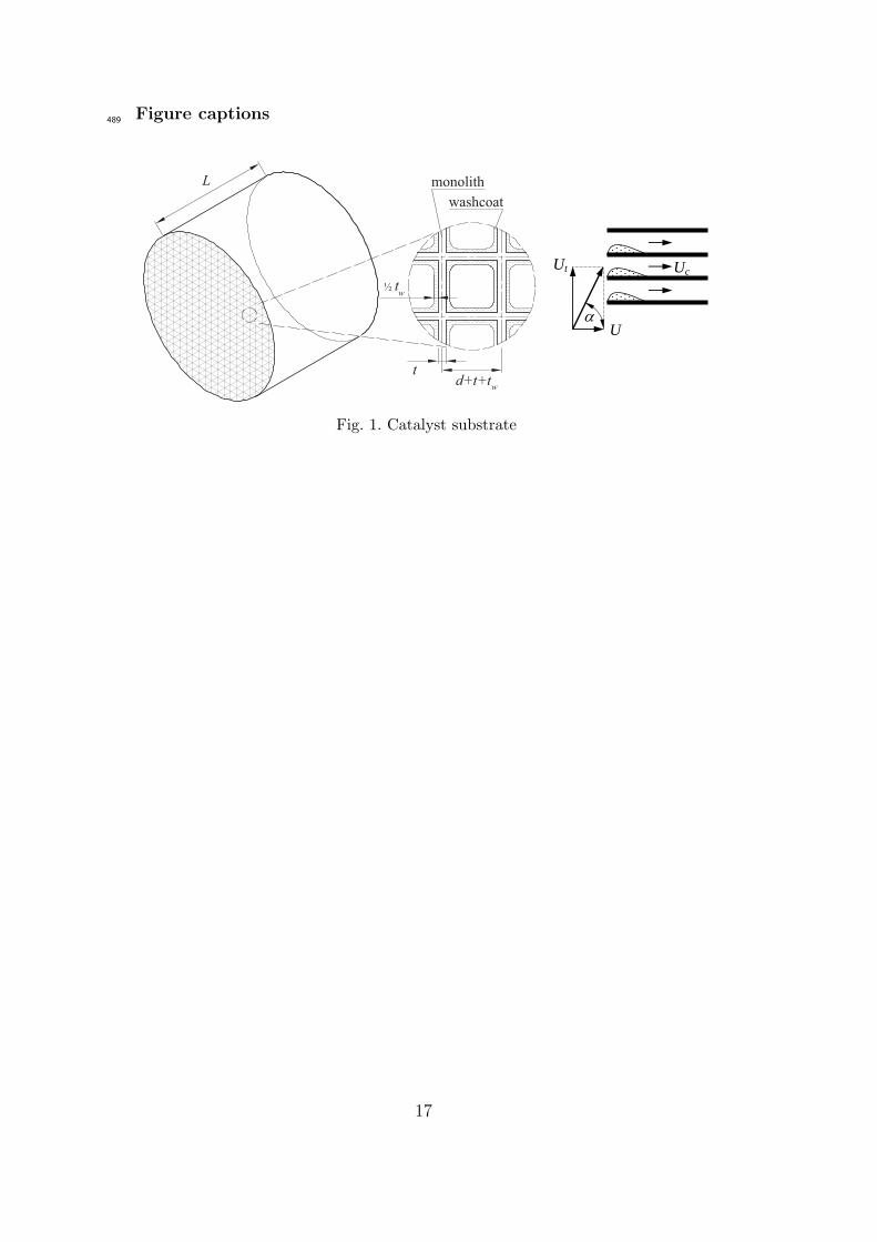
Figure captions489

x

Lz

y

td+t+t

monolith

washcoat

½ tw

w

α U

Ut Uc

Fig. 1. Catalyst substrate

17

(a)Rootsblower

∆pp , t

flow rateorifice

adjustable swirl

swirl generator + annular duct

L L

L

∆poo o

a

p

*

(b)

θ

x

r

V

U

Wpositive

swirl viewing glass

L

RRi

W'

UU'β

r

x

rx 2φ

Fig. 2. Annular swirling flow rig: (a) overview and (b) detail of the measurementsection

18

0.75 0.8 0.85 0.9 0.95 10

0.5

1

1.5

r / R (−)

Vel

ocity

, pre

ssur

e (−

)

L / d = 22.4, SW = 0.00, x = −0.5 D

U/Um (U

m = 13.8 ± 0.11 m/s)

W/Um (W

m = 0.1 ± 0.05 m/s), S = 0.01 ± 0.65

∆p/∆pwall

(∆pwall

= 314 ± 1 Pa)

(a)

0.75 0.8 0.85 0.9 0.95 10

0.5

1

1.5

r / R (−)

Vel

ocity

, pre

ssur

e (−

)

L / d = 22.4, SW = 0.60, x = −0.5 D

U/Um (U

m = 14.6 ± 0.04 m/s)

W/Um (W

m = 3.6 ± 0.02 m/s), S = 0.22 ± 0.01

∆p/∆pwall

(∆pwall

= 323 ± 1 Pa)

(b)

0.75 0.8 0.85 0.9 0.95 10

0.5

1

1.5

r / R (−)

Vel

ocity

, pre

ssur

e (−

)

L / d = 22.4, SW = 0.90, x = −0.5 D

U/Um (U

m = 13.8 ± 0.05 m/s)

W/Um (W

m = 6.5 ± 0.03 m/s), S = 0.42 ± 0.01

∆p/∆pwall

(∆pwall

= 337 ± 1 Pa)

(c)

0.75 0.8 0.85 0.9 0.95 10

0.5

1

1.5

r / R (−)

Vel

ocity

, pre

ssur

e (−

)L / d = 22.4, SW = 1.00, x = −0.5 D

U/Um (U

m = 14.4 ± 0.05 m/s)

W/Um (W

m = 9.1 ± 0.04 m/s), S = 0.56 ± 0.01

∆p/∆pwall

(∆pwall

= 352 ± 1 Pa)

(d)

Fig. 3. Radial profile of velocity [U,W ] and pressure p at x = −0.5D, upstream ofL = 26 mm substrate, for swirl setting (a) 0%, (b) 60%, (c) 90% and (d) 100%

19

−2 −1.5 −1 −0.5 00

0.5

1

1.5

x / D (−)

Vel

ocity

(−

)

L / d = 22.4, SW = 0.00, r = R*

U/Um (U

m = 15.3 ± 0.07 m/s)

W/Um (W

m = 0.2 ± 0.05 m/s)

(a)

−2 −1.5 −1 −0.5 00

0.5

1

1.5

x / D (−)

Vel

ocity

(−

)

L / d = 22.4, SW = 1.00, r = R*

U/Um (U

m = 15.3 ± 0.14 m/s)

W/Um (W

m = 9.3 ± 0.13 m/s)

(b)

−2 −1.5 −1 −0.5 00

0.5

1

1.5

x / D (−)

Vel

ocity

(−

)

L / d = 43.9, SW = 0.00, r = R*

U/Um (U

m = 16.5 ± 0.03 m/s)

W/Um (W

m = 0.6 ± 0.02 m/s)

(c)

−2 −1.5 −1 −0.5 00

0.5

1

1.5

x / D (−)

Vel

ocity

(−

)L / d = 43.9, SW = 1.00, r = R*

U/Um (U

m = 16.3 ± 0.07 m/s)

W/Um (W

m = 10.3 ± 0.05 m/s)

(d)

Fig. 4. Axial profile of velocity [U,W ] at r = R∗ = (Ri + R)/2, upstream of(a,b) L = 26 mm and (c,d) L = 51 mm substrate, for swirl setting (a,c) 0%,(b,d) 100%

20

r

R R Ri*

VVmax

D/2

x

UU∞

x 0

ΔU

Fig. 5. Scaling analysis of radial spreading near the catalyst substrate inlet face

21

0.75 0.8 0.85 0.9 0.95 10

0.5

1

1.5

r / R (−)

Vel

ocity

(−

)

L / d = 22.4, SW = 0.00, x = L+1 mm

U/Um

(Um

= 16.5 ± 0.15 m/s)

(a)

0.75 0.8 0.85 0.9 0.95 10

0.5

1

1.5

r / R (−)

Vel

ocity

(−

)

L / d = 22.4, SW = 1.00, x = L+1 mm

U/Um

(Um

= 16.0 ± 0.17 m/s)

(b)

Fig. 6. Radial profile of velocity U at x = L + 1 mm, downstream of L = 26 mmsubstrate, for swirl setting (a) 0% and (b) 100%

22

0 0.2 0.4 0.6 0.8 10

0.1

0.2

0.3

0.4

0.5

Tangential velocity Wmax

/Um

(−)

Kα (

−)

Kα = 0.459 (Wmax

/Um

)2 (±13%), R2 = 0.81

L / d = 4.3L / d = 9.9L / d = 22.4L / d = 43.9

Fig. 7. Oblique inlet pressure loss Kα versus tangential velocity W , for substratelengths 4.3 6 L/d 6 44

23

0 0.2 0.4 0.6 0.8 10

0.1

0.2

0.3

0.4

0.5

Tangential velocity Wmax

/Um

(−)

Kα (

−)

Kα = 0.459 (Wmax

/Um

)2 (±13%), R2 = 0.81

Kα(1) = tan2α

Kα(2) = tan2α − K

0 (L/d = 10)

Fig. 8. Oblique inlet pressure loss Kα in comparison to K(1)α and K

(2)α [8]

24