observing mass transport to understand global change and
TRANSCRIPT

Deutsche Geodätische Kommission
der Bayerischen Akademie der Wissenschaften
Reihe B Angewandte Geodäsie Heft Nr. 320
Observing Mass Transportto Understand Global Change and to Benefit Society:
Science and User Needs
– An international multi-disciplinary initiative for IUGG –
edited by
Roland Pail
with contributions of
Rory Bingham, Carla Braitenberg, Annette Eicker, Martin Horwath, Eric Ivins, Laurent Longue-vergne, Isabelle Panet, Bert Wouters, Gianpaolo Balsamo, Melanie Becker, Decharme Bertrand,John D. Bolten, Jean-Paul Boy, Michiel van den Broeke, Anny Cazenave, Don Chambers, Tonievan Dam, Michel Diament, Albert van Dijk, Henryk Dobslaw, Petra Döll, Jörg Ebbing, JamesFamiglietti, Wei Feng, Rene Forsberg, Nick van de Giesen, Marianne Greff, Andreas Güntner, Jun-Yi Guo, Shin-Chan Han, Edward Hanna, Kosuke Heki, György Hetényi, Steven Jayne, WeipingJiang, Shuanggen Jin, Georg Kaser, Matt King, Armin Köhl, Harald Kunstmann, Jürgen Kusche,Thorne Lay, Anno Löcher, Scott Luthcke, Marta Marcos, Mark van der Meijde, Valentin Mikhailov,Christian Ohlwein, Fred Pollitz, Yadu Pokhrel, Rui Ponte, Matt Rodell, Cecilie Rolstad-Denby,Himanshu Save, Bridget Scanlon, Sonia Seneviratne, Frederique Seyler, Andrew Shepherd, TonySong, Wim Spakman, C.K. Shum, Holger Steffen, Wenke Sun, Qiuhong Tang, Virendra Tiwari,Isabella Velicogna, John Wahr, Wouter van der Wal, Lei Wang, Hua Xie, Hsien-Chi Yeh, Pat Yeh,Ben Zaitchik, Victor Zlotnicki
München 2015
Verlag der Bayerischen Akademie der Wissenschaften
in Kommission beim Verlag C. H. Beck
ISSN 0065-5317 ISBN 978-3-7696-8599-2


Deutsche Geodätische Kommission
der Bayerischen Akademie der Wissenschaften
Reihe B Angewandte Geodäsie Heft Nr. 320
Observing Mass Transportto Understand Global Change and to Benefit Society:
Science and User Needs
– An international multi-disciplinary initiative for IUGG –
edited by
Roland Pail
with contributions of
Rory Bingham, Carla Braitenberg, Annette Eicker, Martin Horwath, Eric Ivins, Laurent Longuevergne,Isabelle Panet, Bert Wouters, Gianpaolo Balsamo, Melanie Becker, Decharme Bertrand, John D. Bolten,Jean-Paul Boy, Michiel van den Broeke, Anny Cazenave, Don Chambers, Tonie van Dam, Michel Diament,Albert van Dijk, Henryk Dobslaw, Petra Döll, Jörg Ebbing, James Famiglietti, Wei Feng, Rene Forsberg,Nick van de Giesen, Marianne Greff, Andreas Güntner, Jun-Yi Guo, Shin-Chan Han, Edward Hanna,Kosuke Heki, György Hetényi, Steven Jayne, Weiping Jiang, Shuanggen Jin, Georg Kaser, Matt King,Armin Köhl, Harald Kunstmann, Jürgen Kusche, Thorne Lay, Anno Löcher, Scott Luthcke, Marta Marcos,Mark van der Meijde, Valentin Mikhailov, Christian Ohlwein, Fred Pollitz, Yadu Pokhrel, Rui Ponte, MattRodell, Cecilie Rolstad-Denby, Himanshu Save, Bridget Scanlon, Sonia Seneviratne, Frederique Seyler,Andrew Shepherd, Tony Song, Wim Spakman, C.K. Shum, Holger Steffen, Wenke Sun, Qiuhong Tang,Virendra Tiwari, Isabella Velicogna, John Wahr, Wouter van der Wal, Lei Wang, Hua Xie, Hsien-Chi Yeh,Pat Yeh, Ben Zaitchik, Victor Zlotnicki
München 2015
Verlag der Bayerischen Akademie der Wissenschaftenin Kommission beim Verlag C. H. Beck
ISSN 0065-5317 ISBN 978-3-7696-8599-2
Adresse der Deutschen Geodätischen Kommission:
Deutsche Geodätische Kommission
Alfons-Goppel-Straße 11 ! D – 80 539 München
Telefon +49 – 89 – 23 031 1113 ! Telefax +49 – 89 – 23 031 - 1283 / - 1100
e-mail [email protected] ! http://www.dgk.badw.de
Adresse des Herausgebers (Stand Oktober 2015):
Prof. Dr.techn. Mag.rer.nat. Roland PailInstitut für Astronomische und Physikalische Geodäsie
Technische Universität MünchenArcisstraße 21
80333 MünchenE-Mail: pail<at>bv.tum.de
Diese Publikation ist als pdf-Dokument veröffentlicht im Internet unter der Adresse /
This volume is published as pdf-document in the internet
<http://dgk.badw.de/index.php?id=10>
© 2015 Deutsche Geodätische Kommission, München
Alle Rechte vorbehalten. Ohne Genehmigung der Herausgeber ist es auch nicht gestattet,die Veröffentlichung oder Teile daraus auf photomechanischem Wege (Photokopie, Mikrokopie) zu vervielfältigen
ISSN 0065-5317 ISBN 978-3-7696-8599-2

3
Contents
Executive Summary ................................................................................................................................. 5
1. Introduction ................................................................................................................................... 11
2. Overarching scientific questions and benefits from satellite gravimetry ..................................... 14
3. Derivation of requirements for main thematic fields ................................................................... 17
3.1 Continental Hydrology........................................................................................................... 18
3.1.1 Societal challenges related to hydrology ...................................................................... 18
3.1.2 Scientific questions and challenges and their relation to gravity field signals .............. 18
3.1.3 Relevant temporal and spatial scales ............................................................................ 20
3.1.4 Achievements and limitations of current gravity missions ........................................... 21
3.1.5 Identification of potential new satellite gravimetry application fields ......................... 24
3.1.6 Added value of individual mission scenarios ................................................................. 27
3.1.7 Definition of theme-specific science requirement ........................................................ 33
3.2 Cryosphere ............................................................................................................................ 35
3.2.1 Societal challenges related to the cryosphere .............................................................. 35
3.2.2 Scientific questions and challenges and their relation to gravity field signals .............. 35
3.2.3 Relevant temporal and spatial scales ............................................................................ 37
3.2.4 Achievements and limitations of current gravity missions ........................................... 40
3.2.5 Identification of potential new satellite gravimetry application fields ......................... 45
3.2.6 Added value of individual mission scenarios ................................................................. 47
3.2.7 Definition of theme-specific science requirement ........................................................ 50
3.3 Oceanography ....................................................................................................................... 52
3.3.1 Societal challenges in oceanography............................................................................. 52
3.3.2 Scientific questions and challenges and their relation to gravity field signals .............. 54
3.3.3 Relevant temporal and spatial scales ............................................................................ 57
3.3.4 Achievements and limitations of current gravity missions ........................................... 58
3.3.5 Identification of potential new satellite gravimetry application fields ......................... 62
3.3.6 Added value of individual mission scenarios ................................................................. 64
3.3.7 Definition of theme-specific science requirement ........................................................ 69
3.4 Solid Earth ............................................................................................................................. 71
3.4.1 Societal challenges related to solid Earth ..................................................................... 71
3.4.2 Scientific questions and challenges and their relation to gravity field signals .............. 72
3.4.3 Relevant temporal and spatial scales ............................................................................ 76

4
3.4.4 Achievements and limitations of current gravity missions ........................................... 77
3.4.5 Identification of potential new satellite gravimetry application fields ......................... 82
3.4.6 Added value of individual mission scenarios ................................................................. 88
3.4.7 Definition of theme-specific science requirement ........................................................ 90
3.5 Cross-theme aspects and additional thematic fields ............................................................ 93
4. Consolidated Science Requirements ............................................................................................. 97
5. Bibliography ................................................................................................................................. 101
5.1 Continental Hydrology (chapter 3.1) ................................................................................... 101
5.2 Cryosphere (chapter 3.2) ..................................................................................................... 106
5.3 Ocean (chapter 3.3) ............................................................................................................. 108
5.4 Solid Earth (chapter 3.4) ...................................................................................................... 111
5.5 Cross-theme aspects and additional thematic fields (chapter 3.5)..................................... 116
Appendix 1: Thematic Expert Panels ................................................................................................... 117
Appendix 2: Previous studies .............................................................................................................. 120
Appendix 3: Performance numbers – Conversion .............................................................................. 121

5
Executive Summary There is a strong science and user need for the sustained observation of the Earth’s gravity field by means of dedicated satellite gravity missions. They provide a unique tool for observing changes and dynamic processes in the Earth system related to mass transport that is complementary to all other types of available and planned Earth observation missions. During the last decade, with satellite gravity missions of the first generation such as GRACE and GOCE, spectacular science results and new insights into the Earth’s sub-systems hydrosphere, cryosphere, oceans, atmosphere and solid Earth, and their interaction, could be achieved. However, these results suffer from several shortfalls, such as limited temporal and spatial resolution and a limited length of the observation time series. The quantification of dynamic processes in the components of the Earth system and of their coupling provides an improved understanding of the global-state behavior of the Earth as well as direct and essential indicators of both subtle and dramatic global change. Therefore, a sustained observation of mass transport at fine scales for long periods is needed and mandatory for separating natural from human-made climate change effects. For the sustained observation of the global water cycle, satellite gravimetry is unique because it observes the completely integrated water column. It also enables the detection of sub-surface storage variations of groundwater or sub-glacial water mass exchanges that are generally difficult to access and that have specifically been hidden from remote sensing observations. Therefore, with satellite gravimetry all relevant processes of the global water cycle and mass changes of ice sheets and glaciers can be quantified, allowing to directly estimate their contribution to sea level rise. Because of its unique sensitivity to the solid Earth interior mass displacement, satellite gravity can also provide important information for monitoring the entire seismic cycle and understanding how stress accumulates and is released. In spite of the great contributions by the first generation of satellite gravity missions, our current knowledge of mass transport and mass variations within the Earth system still has severe gaps. Due to a currently achievable resolution of 200-500 km (depending on signal strength, time scale and geographic location) on a monthly basis, worldwide only about 10% of the hydrological basins can be captured, and not even the largest individual outlet glacier drainage basins of ice sheets can be resolved. This limited spatial resolution also hampers the separation of different superimposed processes, thus leading to leakage problems and the misinterpretation of signals. As an example, current uncertainties in the knowledge of glacial isostatic adjustment (GIA), resulting from deglaciation of primarily ice sheets, overprint ice mass variations in Antarctica. For ocean applications, a higher spatial resolution and measurement accuracy is required to monitor the variability of the main processes driving ocean circulation, such as the Atlantic Meridional Overturning Circulation (AMOC). Due to limited measurement accuracy, up to now only the very strongest earthquakes with a magnitude greater than 8.4 can be detected. Many applications also suffer from the limited length of the currently available time series. More reliable separation of anthropogenic and naturally induced changes of the water cycle, ice mass melting and sea level rise on global to regional scales requires a sustained observation infrastructure. Natural processes like decadal fluctuation of Earth’s global mean surface temperature obscure, and therefore make it difficult to predict, secular anthropogenic change in climate. The currently too short time series prevent us from disentangling the effect of climate

6 Executive Summary
modes on global and regional sea level. Limited temporal and spatial resolution together with rather long product latencies hamper the use of satellite gravity products for near real time applications and services. The current shortcoming of the gravity observation infrastructure can be overcome by tackling the following challenges in the future.
A long-term sustained satellite gravity observation system is a prerequisite for deriving robust and reliable trend estimates and for capturing non-secular behavior. At least 3 decades of gravity time series are required for properly separating true secular changes from natural mass transport variability wherein we anticipate a rich spectrum of scales to be operating. The longer the time series, the better positioned we are to provide answers to questions of ice mass loss, sea level rise, groundwater depletion, and natural hazards. The longer time series will also allow identifying the intensification of seasonal transport of mass and energy, say between the tropics and sub-tropics. Therefore, the continuation of available time series is of utmost importance.
Increase of spatial resolution, targeting approximately 100 km, is required to properly monitor important catchment basins that are either smaller than, or at the resolution limits of, current space gravimetric missions. It is a prerequisite to study hydrological and cyrospheric processes on regional and sub-basin scale, to include regional ocean mass and heat transport patterns into empirical forecasts of sea level rise and coastal vulnerability, and it will also facilitate separation of superimposed signals. Moreover, it will close the scaling gap to high-resolution terrestrial data and will thus enable consistent combination with complementary in-situ terrestrial and remote sensing observations.
Increase of temporal resolution toward 1 to a few days, in combination with short latencies, will facilitate real-time application services, such as in water management and evaluation of flood risk or agricultural and ecosystem stress, and the inclusion of satellite gravity data into operational forecasting. An increased temporal resolution will also provide data related to more complex modes, such as quasi-periodic stability and unstable transitions in climate physics.
Consistent combination of satellite gravimetry with complementary satellite and ground-based data will provide a more complete picture of Earth system processes. It is necessary to separate mass and thermosteric effect of sea level change, to measure global ocean circulation to disentangle the individual contributors to the global water cycle and to close the water budget, to quantify the flux exchange between land and atmosphere, and to separate solid Earth processes from ice mass changes.
Combined observations and their uncertainties have to be assimilated and consistently integrated into physical process models, because the physical understanding of processes forms the basis to facilitate reliable predictions. The long-term aim is to feed an Earth system model directly with mass changes rather than to extract each contributing source as it is done today. The integration of sustained mass transport observations will result in improvements in climate system models, and will provide an important and unique variable for global initiatives such as the Intergovernmental Panel on Climate Change (IPCC).
Meeting these challenges, the sustained high-resolution mapping of mass transport for a long period will help solving the following science objectives, among others,
� Closure of the global water balance on scales down to 150-200 km and separation of medium-scale drainage basins,

7
� Robust estimation of ice mass balance for individual drainage basins at monthly to decadal time-scales, their relation to climate forcing and their contribution to global and regional sea level rise,
� Recovery of variations in global ocean circulation patterns, as well as mass and heat transport in the oceans on regional scale,
� Regional separation of mass and steric contributions to regional and global sea level rise, � Monitoring earthquake events with magnitude M > 7.0 (about 12 events per year), � Signal separation of tectonic, GIA, hydrologic and cryospheric effects, � Support of atmospheric modelling by observing processes related to surface mass balance
changes, � Separation of natural and human-made effects of climate change on regional scale.
A stronger commitment to turn satellite gravimetry into an observation system would enable to include gravimetric data sets into operational modelling and forecasting systems. Ensuring short latencies of data availability, significant contributions to applications of water management, short-term prediction and operational forecasting of floods and droughts, risk management and disaster mitigation related to natural hazards, and monitoring changes of a globally unified height reference surface for land management applications will serve important societal needs. Understanding the dynamics of coastal sea level variability will support medium-term forecasting of coastal vulnerability, and understanding the climate forcing on continental hydrology, cryosphere, ocean and atmosphere will enable significant contributions to near-future climate predictions. Fig. E-1 summarizes the main scientific (yellow) and societal (blue) objectives addressed by a future satellite gravity constellation.
Figure E-1: Main scientific (yellow) and societal (blue) objectives addressed by a future sustained satellite gravity observing system.
8 Executive Summary
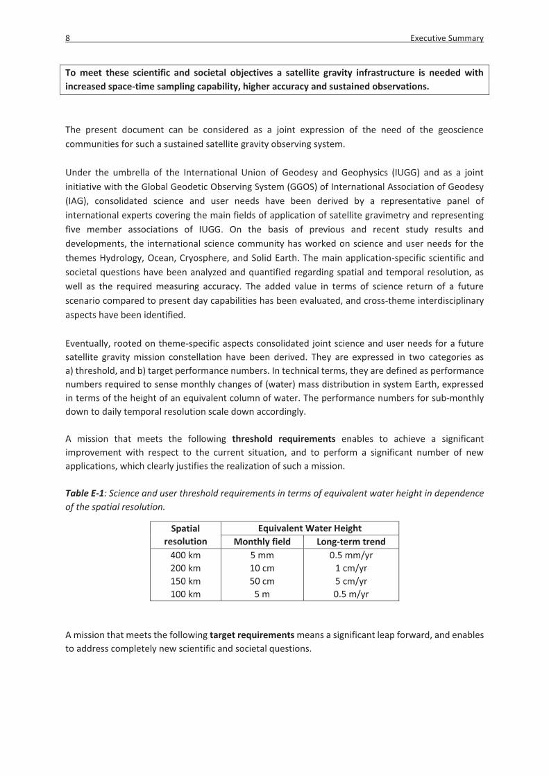
To meet these scientific and societal objectives a satellite gravity infrastructure is needed with increased space-time sampling capability, higher accuracy and sustained observations. The present document can be considered as a joint expression of the need of the geoscience communities for such a sustained satellite gravity observing system. Under the umbrella of the International Union of Geodesy and Geophysics (IUGG) and as a joint initiative with the Global Geodetic Observing System (GGOS) of International Association of Geodesy (IAG), consolidated science and user needs have been derived by a representative panel of international experts covering the main fields of application of satellite gravimetry and representing five member associations of IUGG. On the basis of previous and recent study results and developments, the international science community has worked on science and user needs for the themes Hydrology, Ocean, Cryosphere, and Solid Earth. The main application-specific scientific and societal questions have been analyzed and quantified regarding spatial and temporal resolution, as well as the required measuring accuracy. The added value in terms of science return of a future scenario compared to present day capabilities has been evaluated, and cross-theme interdisciplinary aspects have been identified. Eventually, rooted on theme-specific aspects consolidated joint science and user needs for a future satellite gravity mission constellation have been derived. They are expressed in two categories as a) threshold, and b) target performance numbers. In technical terms, they are defined as performance numbers required to sense monthly changes of (water) mass distribution in system Earth, expressed in terms of the height of an equivalent column of water. The performance numbers for sub-monthly down to daily temporal resolution scale down accordingly. A mission that meets the following threshold requirements enables to achieve a significant improvement with respect to the current situation, and to perform a significant number of new applications, which clearly justifies the realization of such a mission. Table E-1: Science and user threshold requirements in terms of equivalent water height in dependence of the spatial resolution.
Spatial resolution
Equivalent Water Height Monthly field Long-term trend
400 km 200 km 150 km 100 km
5 mm 10 cm 50 cm
5 m
0.5 mm/yr 1 cm/yr 5 cm/yr 0.5 m/yr
A mission that meets the following target requirements means a significant leap forward, and enables to address completely new scientific and societal questions.

9
Table E-2: Science and user target requirements in terms of equivalent water height in dependence of the spatial resolution.
Spatial resolution
Equivalent Water Height Monthly field Long-term trend
400 km 200 km 150 km 100 km
0.5 mm 1 cm 5 cm 0.5 m
0.05 mm/yr 0.1 cm/yr 0.5 cm/yr 0.05 m/yr
Recommendation: The international science community, represented by IUGG, urges international and national institutions, agencies and governmental bodies in charge of supporting Earth science research to make all efforts in implementing a long-term satellite gravity observing system with high accuracy that would respond to the aforementioned need for sustained observation.

10

11
1. Introduction Global satellite gravity measurements provide unique information on mass and mass transport processes in system Earth. They are linked to changes and dynamic processes in continental hydrology, cryosphere, oceans, atmosphere, and solid Earth. Investigation of the non-tidal time-dependence of the Earth’s gravity field began with the launch of Starlette in 1975, and Lageos-1 in 1976. While of great scientific value, orbital tracking of these satellites have mapping capability at very large scales (only up to wavelengths of the order of the radius of the Earth), and therefore had either limited, or virtually no application to mass transport studies. Some 25 years later, however, dedicated gravity missions such as CHAMP (Challenging Minisatellite Payload), GRACE (Gravity Recovery And Climate Experiment) and GOCE (Gravity field and Steady-State Ocean Circulation Explorer) initiated a revolution in our understanding of near-surface mass transport processes due to the improved resolution to medium scales offered by these global gravity field mapping missions. A future gravity field observation concept at even finer scales is expected to realize a similarly dramatic advancement in application capabilities and scientific discoveries. Therefore, it is important to address mission concepts beyond those of the GRACE-Follow-On mission that is scheduled for launch in 2017 and to move from demonstration capabilities to sustained observations at fine scale whilst continuing the medium scale heritage from GRACE and GRACE Follow-on. Beyond scientific questions, a future satellite gravity constellation shall be able to address practical applications with societal benefit. Figure 1 summarizes the main scientific (yellow) and societal (blue) challenges that shall be tackled by such a future concept.
Figure 1-1: Main scientific (yellow) and societal (blue) challenges addressed by a future satellite gravity constellation.

12 1 Introduction
Previous studies on selected science needs and mission goals (see Appendix 2) have resulted in quite different performance requirements for future gravity concepts. Therefore, the main motivation of this initiative is to collect all relevant scientific and user communities’ needs and to achieve consensus on expected and desired performance of a future satellite gravity field concept, which is capable of serving these needs. Furthermore, it can expand our knowledge of global mass transport processes at short and long time-scales within the Earth system and in the meantime provide sustained observations of this essential global change variable. Therefore, in a joint initiative of the International Union of Geodesy and Geophysics (IUGG), the Global Geodetic Observing System (GGOS) (Working Group on Satellite Missions), and the International Association of Geodesy (IAG) (Sub-Commissions 2.3 and 2.6), consolidated science and user needs have been derived by a representative panel of international experts covering the main fields of application of satellite gravimetry (cf. Appendix 1). They are representing five member associations of IUGG: International Association of Hydrological Sciences (IAHS), International Association for the Physical Sciences of the Oceans (IAPSO), International Association of Cryospheric Sciences (IACS), International Association of Seismology and Physics of the Earth's Interior (IASPEI), and International Association of Geodesy (IAG), with additional contributions by the International Association of Meteorology and Atmospheric Sciences (IAMAS).
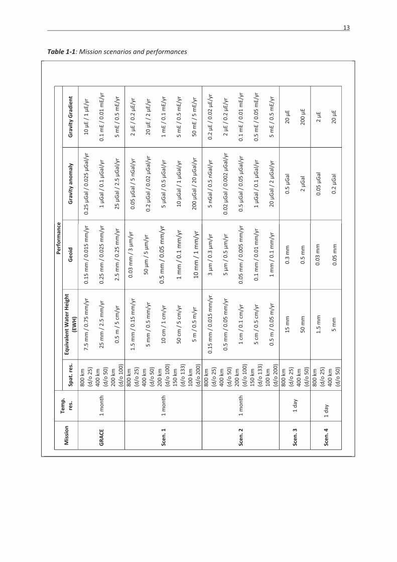
On the basis of previous and recent study results and developments, the international science community has worked on science and user needs for the themes Hydrology, Ocean, Cryosphere, and Solid Earth. In order to guide the discussion between what is desired and what might be feasible whilst keeping technological capability in mind, a limited number of mission scenarios have been assessed to see which science and user needs can be addressed roughly by what type of mission (cf. Table 1-1). This is done to trade-off new applications and the added value in terms of science return of a future scenario compared to present day capabilities.
The logical flow of this document is as follows: In Chapter 2, the overarching scientific questions of global mass transport in the climate system that can be addressed by satellite gravimetry are discussed. In Chapter 3, the science requirements for the four main themes, hydrology, cryosphere, ocean, and solid Earth, are derived, and cross-theme interdisciplinary aspects are identified. Finally, in Chapter 4, a set of consolidated science and user requirements are derived from those rooted in the four themes. Consensus on these requirements has been achieved at a joint international workshop that was held on 26-27 September 2014 in Herrsching/München, Germany.
Therefore, the resulting consolidated Science and User Need Document can be considered as a joint expression of the need of the geoscience communities for a future sustained satellite gravity field infrastructure.
13
Table 1-1: Mission scenarios and performances
Mis
sion
Te
mp.
re
s.
Perf
orm
ance
Spat
. res
. Eq
uiva
lent
Wat
er H
eigh
t (E
WH)
G
eoid
G
ravi
ty a
nom
aly
Gra
vity
Gra
dien
t
GRA
CE
1 m
onth
800
km
(d/o
25)
40
0 km
(d
/o 5
0)
200
km
(d/o
100
)
7.5
mm
/ 0.
75 m
m/y
r
25 m
m /
2.5
mm
/yr
0.
5 m
/ 5
cm/y
r
0.15
mm
/ 0.
015
mm
/yr
0.
25 m
m /
0.02
5 m
m/y
r
2.5
mm
/ 0.
25 m
m/y
r
0.25
μGa
l / 0
.025
μGa
l/yr
1
μGal
/ 0.
1 μG
al/y
r
25 μ
Gal /
2.5
μGa
l/yr
10 μ
E / 1
μE/
yr
0.
1 m
E / 0
.01
mE/
yr
5
mE
/ 0.5
mE/
yr
Scen
. 1
1 m
onth
800
km
(d/o
25)
40
0 km
(d
/o 5
0)
200
km
(d/o
100
) 15
0 km
(d
/o 1
33)
100
km
(d/o
200
)
1.5
mm
/ 0.
15 m
m/y
r
5 m
m /
0.5
mm
/yr
10
cm
/ 1
cm/y
r
50 c
m /
5 cm
/yr
5
m /
0.5
m/y
r
0.03
mm
/ 3
μm/y
r
50 μ
m /
5 μm
/yr
0.
5 m
m /
0.05
mm
/yr
1
mm
/ 0.
1 m
m/y
r
10 m
m /
1 m
m/y
r
0.05
μGa
l / 5
nGal
/yr
0.
2 μG
al /
0.02
μGa
l/yr
5
μGal
/ 0.
5 μG
al/y
r
10 μ
Gal /
1 μ
Gal/y
r
200
μGal
/ 20
μGa
l/yr
2 μE
/ 0.
2 μE
/yr
20
μE
/ 2 μ
E/yr
1 m
E / 0
.1 m
E/yr
5 m
E / 0
.5 m
E/yr
50 m
E / 5
mE/
yr
Scen
. 2
1 m
onth
800
km
(d/o
25)
40
0 km
(d
/o 5
0)
200
km
(d/o
100
) 15
0 km
(d
/o 1
33)
100
km
(d/o
200
)
0.15
mm
/ 0.
015
mm
/yr
0.
5 m
m /
0.05
mm
/yr
1
cm /
0.1
cm/y
r
5 cm
/ 0.
5 cm
/yr
0.
5 m
/ 0.
05 m
/yr
3 μm
/ 0.
3 μm
/yr
5
μm /
0.5
μm/y
r
0.05
mm
/ 0.
005
mm
/yr
0.
1 m
m /
0.01
mm
/yr
1
mm
/ 0.
1 m
m/y
r
5 nG
al /
0.5
nGal
/yr
0.
02 μ
Gal /
0.0
02 μ
Gal/y
r
0.5
μGal
/ 0.
05 μ
Gal/y
r
1 μG
al /
0.1
μGal
/yr
20
μGa
l / 2
μGa
l/yr
0.2
μE /
0.02
μE/
yr
2
μE /
0.2
μE/y
r
0.1
mE
/ 0.0
1 m
E/yr
0.5
mE
/ 0.0
5 m
E/yr
5 m
E / 0
.5 m
E/yr
Scen
. 3
1 da
y
800
km
(d/o
25)
40
0 km
(d
/o 5
0)
15 m
m
50
mm
0.3
mm
0.5
mm
0.5
μGal
2 μG
al
20 μ
E
200
μE
Scen
. 4
1 da
y
800
km
(d/o
25)
40
0 km
(d
/o 5
0)
1.5
mm
5 m
m
0.03
mm
0.05
mm
0.05
μGa
l
0.2
μGal
2 μE
20 μ
E
14 2 Overarching scientific questions and benefits from satellite gravimetry
2. Overarching scientific questions and benefits from satellite gravimetry The past decade of satellite gravimetric data - that have so advanced our quantitative understanding of Earth mass transport and mass redistribution processes - demonstrates that the measurement of gravity from space provides both immediate and long-term benefits for society. An improved understanding of the global-state behavior of the Earth and the coupling between dynamic processes of the main components of the Earth system is a central focus for space gravimetry missions. The coupling takes place between elements of ocean, continental hydrology, cryosphere, atmosphere and solid Earth, and these interact through forcing and feedback mechanisms. Satellite gravimetry is a unique measurement technique sensitive to distributed mass and mass change in the Earth system, which includes for example key contributions from the global water cycle. As such, it now has a proven capability to observe processes that are direct indicators of both subtle and dramatic climate change and provide the seed information for improving climate system models. With such improvements we have a better chance to separate natural variability from anthropogenically induced climate changes. Results derived from gravity missions have been widely used as important input for the Intergovernmental Panel on Climate Change (IPCC) Fifth Assessment Report (AR5) in 2014.
Changes in the Earth system occur on a variety of spatial and temporal scales. Currently, they are usually investigated and modelled on the level of individual sub-systems, without fully taking into account the global, large-scale coupling with other sub-systems, feedback-loops and the input/output balance, thus neglecting mass conservation in the total system. Therefore, consistency of the global mass balance and sea level budget are key scientific challenges to obtain a consistent picture of the Earth system and its changes.
Most of the mass redistribution processes are related to the global water cycle, by which the ocean, atmosphere, land, and cryosphere storages of water interact through temporal and spatial water mass variations, at time scales ranging from daily to inter-annual, and decadal periods. Examples of mass changes related to climate variability are ice mass changes in ice sheets, ice caps and glaciers, changes in the global ocean circulation patterns, sea level rise, ground water storage change and severe droughts. These processes may indicate a change in forcing or of feedback loops that have an impact on climate change. Therefore, mass variations in all sub-systems can be considered as a proxy and indicator for natural or anthropogenic-induced climate change.
The understanding of the dynamics and the variations of the global water cycle requires the closing of the water balance, i.e. the variation of water mass input, output and storage in time and space, and a solid understanding of the processes governing the water exchange between all sub-systems: land, oceans, ice masses, and the atmosphere. Today, many processes are still poorly understood, which is also due to the fact that they are hardly accessible through direct measurements. For example, almost no direct observational techniques for evapotranspiration and for storage changes in groundwater and deep aquifers exist for large areas. Also, other water flux terms of the continental water budget (precipitation, run-off) have been provided with large uncertainties only. It has been difficult if not impossible to validate global hydrological models until space gravimetry data became available. Time-lapse gravity observations are an integral measure of water storage changes. These observations have the potential to close the terrestrial water budget, and they serve as an important constraint to evaluate and complement observed and modeled fluxes, provided that they are available with sufficiently high temporal and spatial resolution. Currently, the size of many river basins is somewhat smaller than the spatial resolution of satellite gravimetry. However, the societal relevance of closing the terrestrial water balance and of observing changes in the water storage lies in providing sound

15
information on changing freshwater supply for human consumption, for agriculture and industry, facing the challenge of steadily growing demands that are anticipated for the future. Thus, gravity data may provide a basis for developing sustainable water resource management strategies, including near real-time observations for the monitoring and prediction of extreme hydrological events such as floods and droughts.
Knowledge on the state of continental ice masses and the processes of past and present evolution of ice sheets and glaciers is also key for the understanding of the Earth and climate system, because they represent very sensitive indicators of climate change. In contrast to other geometrical observation methods, satellite gravimetry is relatively little affected by problems of incomplete sampling and avoids the inherent difficulty of making problematic ice volume to mass conversions (firnification). However, the shortness of available time series still makes it difficult to separate anthropogenic-induced effects from natural long-term variability, and the current observation capabilities via GRACE with limited spatial scales of 200-500 km (depending on signal strength, time scale and geographic location) restrict their application to larger catchments. Consequently, the current understanding of cryospheric mass balance and coupling processes, such as the dynamic response of ice flow to changing oceanic and atmospheric boundary conditions and interactions with subglacial hydrology, remains limited.
Interaction of continental hydrology and cryosphere with the ocean results in changes in the mean sea level, as the sum of mass in(out)flux and a thermosteric component. With the help of gravity observations, a separation between these two components can be achieved on global to regional level, and the individual contributions can be quantified. The monitoring and prediction of sea level change has an important societal impact to address coastal vulnerability and for the mitigation and adaptation of global coastal industrial infrastructure. Additionally, in combination with complementary data sources, surface and deep ocean circulation, the latter being an essential but hidden part of the climate system, can be quantified, and thus we have the possibility to greatly improve models of the energy transport in the oceans, atmosphere and land hydrosphere. Closing the sea level budget still poses a great challenge due to that fact that complementary observations of dissimilar temporal and spatial character and of entirely differing sampling, error budgets and bias corrections must be dealt with.
The solid Earth experiences mass variability associated with its deformation. The associated time scales vary: viscous deformations are slow and reveal themselves primarily as trends, and elastic deformations are short-term processes associated with great earthquakes, which are essentially instantaneous step jumps. Glacial Isostatic Adjustment (GIA) is due to long-term viscoelastic rebound of the solid Earth resulting from the deglaciation of primarily the Late Pleistocene ice sheets, and results in variations of the relative sea level. Thus it is an important example for the coupling of solid Earth with cryosphere and oceans. Together with this viscoelastic deformation, elastic response of the Earth due to loading effects related to changing surface water, ice and atmospheric masses as well as the co- and post-seismic solid Earth deformation hold important information about the Earth’s rheology. In the gravimetry observations, solid Earth mass variations are superimposed on those that are fluid in nature. Consequently, this mixing of signals, part of which have a solid Earth origin, requires careful treatment. This is especially true when trying to interpret climate trend signals, which must be separated from the trend signals related to GIA and tectonic uplift. Accurate model representation of the solid Earth signal can be crucial for deriving precise estimates of continental water and cryospheric mass balance and sea level changes. In the future, it also might be possible to detect mass change signals due to plate tectonics, rising mantle plumes, dynamical processes in the mantle and core motions, which are currently too small to be observed. Finally, in addition to the mitigation of natural hazards and an improved understanding of geophysical processes, also the exploration and evolution

16 2 Overarching scientific questions and benefits from satellite gravimetry
of natural resources, such as minerals, hydrocarbons or geothermal energy, pose a great challenge with a high societal relevance.
In spite of the great contributions by the first generation of satellite gravimetry missions, our knowledge of mass transport and mass variations within the Earth system still has severe gaps, which simultaneously poses challenges to be tackled by satellite gravimetry in the future.
Long-term monitoring is a prerequisite for deriving reliable trend estimates and for capturing non-secular behavior. The longer time-series could provide necessary information for properly separating true secular changes from natural mass transport variability wherein we anticipate a rich spectrum of scales to be operating. The longer the time series, the better positioned we are to providing answers to questions of ice mass loss, sea level rise, groundwater depletion, and natural hazards. The longer time series could also allow identification of the intensification of seasonal transport of mass and energy, say between the tropics and sub-tropics. Therefore, the continuation of available time series is of utmost importance.
Increase of spatial resolution is required to properly monitor important catchment basins that are either smaller than, or at the resolution limits of, current space gravimetric missions. Currently, different spatial scales prevent a consistent combination with complementary in-situ terrestrial and remote sensing observations. An increased spatial resolution will also facilitate signal separation and reduction of leakage effects (contamination of target signals by mass variations in adjacent areas).
Increase of temporal resolution, in combination with short latencies, will facilitate real-time applications and services with direct applicability, e.g., in water management and evaluation of flood risk, issues of coastal vulnerability, and agricultural and ecosystem stress. An increased temporal resolution will also provide data related to more complex modes, such as quasi-periodic stability and unstable transitions in climate physics.
Consistent combination of satellite gravimetry with complementary satellite and ground-based data will provide a more complete picture of Earth system processes. It is necessary to separate mass and thermosteric effect of sea level change, to measure global ocean circulation, to disentangle the individual contributors to the global water cycle and to close the water budget.
Combined observations and their uncertainties have to be assimilated and consistently integrated into physical process models, because the physical understanding of processes forms the basis to facilitate reliable predictions. The long-term aim is to feed an Earth system model directly with mass change observations rather than to extract each contributing source as it is done today.

17
3. Derivation of requirements for main thematic fields In the following, specific requirements for the main fields of application, continental hydrology, cryosphere, ocean, and the solid Earth, are derived. An overview of scientific questions and challenges of each discipline is given, and the spatial and temporal scales of the geophysical phenomena involved are addressed. By necessity we both highlight current achievements and identify certain limitations of satellite gravimetry. Additionally, potential new fields of application and recipes for addressing new research questions are considered. We therefore identify key areas where the limited performance of current missions limits the scope of science questions that we can address. Based on this review and the mission scenarios defined in Chapter 1, the added value of these new mission scenarios is analyzed, based on which theme-specific science and user needs are defined. In this document, we consistently distinguish between threshold requirements and target requirements, which are defined as follows:
� A mission that meets the threshold requirements enables to achieve a significant improvement with respect to the current situation, and to perform a significant number of new applications, which clearly justifies the realization of such a mission.
� A mission that meets the target requirements means a significant leap forward, and enables to address completely new scientific and societal questions.
Finally, based on the theme-specific user needs identified by the main fields of application, joint science and user needs will be derived in Chapter 4.
18 3 Derivation of requirements for main thematic fields
3.1 Continental Hydrology 3.1.1 Societal challenges related to hydrology
The terrestrial hydrological cycle is constantly changing under the influence of natural climate variability, climate change, and direct and indirect anthropogenic impacts. Monitoring, separating and understanding these effects will pose important challenges for hydrological research in the upcoming decades, with critical questions on freshwater resources, food security and ecosystem services preservation (Gerten et al., 2013). In this context, the following societal challenges can be identified:
� Water management The sustainable exploitation of water resources is one of the most important environmental and socio-economic challenges of a constantly growing population, important to ensure drinking water supply, agriculture and food security particularly in arid and semi-arid regions around the world. Terrestrial water storage data based on time-variable gravity monitor overall variations of continental water storage, including all storage compartments such as soil moisture, groundwater, snow and ice, water in rivers/lakes and reservoirs. Therefore, they reflect the abundance of both green and blue water resources, being national or trans-boundary. The sustainable use of water can be investigated and therefore information to evaluate water policies and constrain their impact on ecosystem services can be provided to stakeholders.
� Early warning for extreme events and risk management Hydrological extremes, such as floods and droughts, represent globally important natural hazards. Observations of water storage change have been shown to improve model predictability and constrain potential trends. Therefore, assimilation of these data into models may lead to a better prediction of extreme events, at seasonal time scales (droughts, floods) and short time scales (floods) and contribute to early-warning systems and the set-up of adaptation strategies.
� Understanding climate change impacts on the water cycle The terrestrial water cycle is responding to climate change (see e.g. Douville et al. (2013), Jung et al. (2010)). Water storage information is critical to assess the impact of changing water fluxes, since it accumulates fluxes over long timescales, and can therefore provide valuable insights for both direct and indirect impacts of climate variability. Main advances encompass (but are not limited to) the separation of natural interannual climate cycles from long-term trends, informing about adaptation strategies to climate variability (impact of irrigation, land-use changes), and investigating the storage components with long transfer time (groundwater, permafrost, glaciers). 3.1.2 Scientific questions and challenges and their relation to gravity field signals
Meeting the societal challenges described above leads to the following scientific questions:
The monitoring of changes in water storages on different spatial and temporal scales will remain a challenging task, especially in those storage compartments that are not well constrained by observations (e.g. groundwater, snow with regard to snow water equivalent). Changes in water storage directly cause variations in the gravity field, and monitoring these changes will spur investigation of new processes, which have so far been difficult to analyze, at spatial scales ranging from regional to global. Such processes include, but are not limited to, groundwater-surface water interactions, storage change in confined and unconfined aquifers, permafrost thawing, erosion and sediment transport, and the contribution of glacier melt to the hydrological cycle.

3.1 Continental Hydrology 19
Different modeling results, reanalyses, and observations are available for different variables of the hydrological and the atmospheric water cycle, but we are still far from closing the budgets on various spatial and temporal scales. Reducing the uncertainties for the individual quantities will be required to converge towards budget closure. Especially the water fluxes (precipitation P, evapotranspiration ET, atmospheric convergence, fresh water exchanges with the ocean (surface & subsurface)) are provided with large uncertainties and these will require better constraints. As the net flux deficit is balanced by changes in the water storage term, observed changes of water mass, as provided by gravity field observations, can serve as such constraints.
Other important hydrological challenges will be involved with the evaluation and control of water management procedures and policies. These procedures, such as the impoundment of reservoirs cause gravity changes on very small temporal and spatial scales (but aggregate to larger scales) and will require near real-time observations that are available after a few days. Other examples for near real-time applications, which might gain increasing importance in the future, is the validation of seasonal climate forecasts and the prediction of extreme events such as flooding. Initial conditions of catchment wetness in terms of soil moisture and aquifer storage are a key to this prediction.
Focusing on longer time scales, the identification of climate change signature and anthropogenic impacts on the hydrological cycle will present an important research question. We are still far from disentangling the overlaying influences that inter-annual natural background climate variability, radiative forcing (e.g. CO2 emission due to fossil burning), and direct and indirect anthropogenic influences have on the terrestrial water cycle. Anthropogenic influences might impact and accelerate the water cycle either directly by use and consumption of “blue water”, as it occurs in case of irrigation or during the construction and management of reservoirs, or indirectly through land use and land cover change, which can have significant influence on the generation of evaporation and run-off and through complex soil-vegetation-atmosphere feedbacks. All these effects directly or indirectly influence the distribution of water masses and thus induce variations in the gravity field. Changes in these anthropogenic impacts might be attributed to change of management practices, human adaption to climate change, and population growth. The quantification of individual natural and human-driven influences, as well as the separation of the different effects will only be possible in a joint effort of combining modeling approaches with a large variety of different observations. Furthermore, observed changes of water mass changes will be necessary to validate decadal climate predictions. Being already a major topic in the meteorological community those days (Meehl et al. 2009, Goddard et al. 2013), decadal prediction attempts to bridge the current gap between seasonal predictions and climate projections.
Finally, reliable hydrological models on various spatial and temporal scales will be indispensable for quantifying changes of the terrestrial water cycle, for understanding the underlying controls, and especially for making reliable predictions into the future. For example, when predicting the impact of climate change on water use, the uncertainties that arise from global hydrological models outweigh by far uncertainties from global circulation models and from emission scenarios (Wada et al., 2013). Therefore, it will be one of the major scientific challenges in the upcoming decades to drive and constrain the development of predictive hydrological models for water management and climate adaption studies. One deficit of hydrological models has been an accurate and reliable evaluation of the storage term. Here, space gravimetry has a huge contribution to improve the models. In order to achieve a more realistic representation of the hydrological processes, and to separate all the different effects mentioned in the paragraphs above, these models will have to incorporate a large variety of complementary observations, e.g. by means of data assimilation and model calibration techniques.

20 3 Derivation of requirements for main thematic fields
3.1.3 Relevant temporal and spatial scales
The spatial and temporal scales associated to the abovementioned processes are summarized in Table 3.1-1, and discussed thereafter. Bubble plots illustrating the spatial scales versus the signal magnitude are shown in Fig. 3.1-1.
Table 3.1-1: Spatial and temporal scales associated to gravity changes relevant to land hydrology investigations.
Signal Time scales Expected signals: temporal variation in equivalent water height (EWH)
Spatial scale
Groundwater storage
years to secular
up to ̴ 2-4 cm EWH/yr on large scales, a few cm more on smaller scales
a few 10 km to ~1000 km
monthly to (inter-) annual
up to 10-20 cm on larger scales, up to 30-40 cm on smaller scales of a few 10 km
same as above
Surface water storage
decades to secular
up to 0.5m/year on large scales ( a few 100 km), up to 1 m/year on smaller scales (a few km)
a few meters up to a few hundred km
monthly to (inter-) annual
up to ~10 m, on different scales
same as above
daily to monthly up to a few meters same as above
Soil moisture
monthly to (inter-) annual
up to ~40 cm a few km up to a few 100 km
hourly to daily linked to precipitation and evapotranspiration (see below)
A few km to a few 100 km
Snow water equivalent
years to secular up to 1 cm/year
a few 10 km to a few 100 km
daily to annual up to several m on small scales, up to ̴50 cm on scales of a few 100 km
a few meters up to several 100 of km
Precipitation hourly to daily up 1 m on small scales, up to a few 10 cm on larger scales
a few km to >100 km
Evapotranspiration hourly to daily up to a few cm a few 100 m to a few 100 km
� Groundwater storage changes: The spatial scales of aquifers range from a few tens of kilometers up to around 1000 km for the largest existing aquifer (Great Artesian Basin). When determining groundwater storage changes from satellite gravimetry, the withdrawal of (fossil) groundwater sources is of particular interest. Magnitudes of trends can lead up to ̴ 2-4 cm EWH/yr on large scales and even more on smaller scales. Monthly to interannual groundwater variations reach from a few cm on larger scales, up to 30-40 cm on smaller scales of a few 10 km.
3.1 Continental Hydrology 21
� Surface water storage change: continental surface waters exist on a large range of spatial scales, from a few meters of river width or lake size up to around 300 km for the largest reservoir (Lake Victoria) and 600 km for the largest lake (Caspian Sea). Monthly variations can be in the order of up to ~10 m on all different spatial scales, whereas long-term trends range from around 0.5 m/year on large scales of a few 100 km, up to ~1 m/year on smaller scales of a few km. In case of the impoundment or drawdown of reservoirs, a few meters of water change can be achieved on very short (daily to weekly) time scales.
� Soil moisture storage change (storage change in the unsaturated zone, including root zone): relevant soil moisture variations can be detected on scales of a few meters up to a few 100 km, with magnitudes of monthly to annual variations in the order of up to 40 cm.
� Change in snow water equivalent: Snow covered areas reach from > 100 m to several hundreds of km. Monthly to seasonal storage changes range from several meters on small scales to ~20 cm on scales of a few hundreds of km. Trends of a few mm/year can be expected on scales of a few 10 km to a few 100 km.
� Precipitation: Water mass changes due to precipitation events happen on very short temporal scales of hours to days, reaching several months in monsoonal regions. The spatial dimension spans areas of a few km to a few 100 km with magnitudes of up to 1 m on small scales and a few tens of cm on larger scales. Precipitation is strongly affected by interannual oceanic teleconnections (e.g. El Nino) and trends may reach 0.5 cm per year.
� Evapotranspiration: Water mass changes due to evaporation can occur on small temporal (daily) time scales, but is generally driven by a seasonal cycle. The magnitude can reach a few cm per day and a few 10 cm for interannual variations (e.g. Sudd wetlands, Nile). Trends are in the order of 0.5 mm per year.
� Vegetation storage (biomass, interception water): storage changes of up to 2 mm are regarded as negligible compared to, e.g., 200 mm soil moisture variations, but indirect effects of varying LAI (leaf area index) on related processes such as evapotranspiration might have an effect on water balance and water redistribution.
3.1.4 Achievements and limitations of current gravity missions
GRACE has, for the first time, provided global observations of large-scale terrestrial water storage variations. Time series of basin-wide averages of water storage changes were computed for large and medium size catchments (Swenson and Wahr 2002, Lettenmaier and Famiglietti 2006) to investigate especially seasonal, inter-annual, and long-term water storage variations (e.g., Tang et al. 2010, Becker et al. 2011, Llovel et al. 2010, Crowley et al. 2006). Tailored processing strategies have allowed to push the limits of the spatial extent of river basins down to a surface area of about 200.000 km2 (Longuevergne et al. 2010) and to investigate smaller-scale mass change phenomena with large amplitude, as they occur, e.g., in case of surface water bodies (Awange et al. 2013, Tourian et al. 2015).
This improved knowledge of water storage changes has allowed to impose innovative constraints on the estimation of water fluxes such as precipitation (Swenson 2010, Seo et al. 2010), evapotranspiration (Ramilien et al. 2006, Long et al. 2014a), the flux deficit (precipitation minus evapotranspiration, Swenson and Wahr 2006) and river discharge (Syed et al. 2007, Syed et al. 2010, Jensen et al. 2013) by solving the terrestrial water balance equation for the quantity of interest. From the opposite point of view, the degree of closure of the terrestrial water budget, which has only

22 3 Derivation of requirements for main thematic fields
become analyzable because GRACE provides the before largely unknown storage change term, can serve as constraint to evaluate the quality of observed and modeled fluxes and storage changes (Sheffield et al. 2009, Gao et al. 2010, Springer et al. 2014, Lorenz et al. 2014). Furthermore, enforcing the water balance closure as a hard constraint has been used to generate an improved estimate of the individual terms of the water budget equation (Sahoo et al. 2011, Pan et al. 2012). By combining terrestrial and atmospheric water balance equations, GRACE has also been applied to investigate atmospheric water budgets (Fersch et al. 2012) and the fate of water in the global hydrological cycle (van Dijk et al. 2014).
Several studies have proven the potential of satellite gravimetry to serve as a sensor for inter-annual climate variabilities. GRACE water storage variations have been linked to ENSO-like climate indices, revealing good correlations in various regions (Garcia-Garcia 2011, Xavier et al. 2010, Morishita et al. 2008, Becker et al. 2010). It has been concluded that GRACE is able to detect all the significant known ENSO teleconnection patterns around the globe (Phillips et al. 2012) and that such teleconnections can also be exploited to predict water storage changes in certain areas (Forootan et al. 2014b).
Furthermore, GRACE time series analysis has enabled the investigation of extreme hydrological events (Seitz et al. 2008, Famiglietti and Rodell 2013, Long et al. 2014b), revealing the capability of GRACE to monitor the spatio-temporal evolution of droughts (Leblanc et al. 2012, Frappart et al. 2012), and floods (Chen et al. 2010b, Espinoza et al. 2013). It was found that GRACE-derived water storage changes provide a more reliable source of information regarding the magnitude of droughts than modeled storages, which often lack an adequate representation of groundwater changes (Chen et al. 2010a, Long et al. 2013). Integrating water storage information into a drought monitoring system has allowed the development of GRACE-based drought indicators and therefore the identification of drought conditions (Hobourg et al. 2012) with the potential to also improve fire season forecasts (Chen et al. 2013). Additionally, it was pointed out that GRACE has the ability to provide unique information on soil saturation conditions and therefore has a considerable potential to be used in flood prediction systems (Reager and Famiglietti 2009, Reager et al. 2014).
As GRACE observes the complete vertically integrated water column, it enables the detection of sub-surface storage variations that are generally difficult to access and that have specifically been hidden from remote sensing observations before. Therefore, it can be considered as one of the major achievements of the GRACE mission, that (anthropogenically induced) groundwater depletion has for the first time been derived from space (Taylor et al 2013). This potential of GRACE has been validated in regions with a good coverage of in-situ groundwater observations, such as North American aquifers (Yeh et al. 2006, Famiglietti et al. 2011, Scanlon et al. 2012) and has been applied to monitor groundwater changes in regions where extensive irrigation is expected to lead to a critical decrease in groundwater resources, such as Northern India (Rodell et al. 2009, Tiwari et al. 2009), the Middle East (Voss et al. 2013, Joodaki et al. 2014, Forootan et al. 2014a, Mulder et al. 2014), the Sahara (Gonçalvès et al. 2013) and Northern China (Feng et al. 2013). In addition to the withdrawal of groundwater, also other direct anthropogenic impacts of water management on the water cycle can be studied using GRACE. As an example, water impoundment in large reservoirs has been quantified from satellite gravimetry and good agreement has been found with in situ measurements of the same surface water storage changes (Wang et al. 2011, Longuevergne et al. 2012).
By providing information on large-scale water storage changes with global coverage, temporal gravity field variations represent an innovative and very valuable data source for the evaluation and improvement of hydrological modeling. A variety of studies have compared modeled and observed storage variations, with the satellite data serving generally as a validation tool for the model output

3.1 Continental Hydrology 23
(e.g., Güntner 2008, Syed et al. 2008, Alkama et al. 2010). Such comparisons have shown that GRACE can detect water storage anomalies which are not sufficiently represented in models (Grippa et al. 2011), and they have revealed the importance of accurately modeling individual storage compartments such as river (Kim et al. 2009), groundwater (Vergnes and Decarme 2012, Pokhrel et al. 2013, Lo et al. 2010), as well as canopy and snow storage compartments (Yang et al. 2011). The validation with GRACE has also illustrated the necessity of correctly representing the lateral redistribution of water (routing) in rivers and groundwater aquifers towards the oceans (Ngo-Duc et al. 2007). Furthermore, a comparison with GRACE trends has led to a more realistic quantification of groundwater withdrawals in groundwater depletion areas world-wide (Döll et al. 2014a). However, it was found that only if water abstractions lead to long-term changes in TWS by depletion or restoration of water storage in groundwater or large surface water bodies, GRACE may be used to support the quantification of human water abstractions (Döll et al. 2014b). In order to improve model structures, calibration approaches have been developed that tune model parameters (retention times, soil water capacities, runoff velocities, etc.) to make the models fit better to GRACE (and other) observations (Werth and Güntner 2010, Xie et al. 2012, Livneh and Lettenmaier 2012). These studies conclude that the resulting calibrated models have better predictability skills and that their output agrees better with independent data sets than the original model runs. Constraining land surface model simulations using GRACE has led to an improved representation of modeled water table depth and therefore to a better characterization of groundwater storage changes (Lo et al. 2010). Recently, it has become increasingly important to assimilate GRACE data into hydrological models, allowing not only for an improvement of model results, but also for a disaggregation of the integral GRACE water storage observations spatially, temporally, and vertically into the individual hydrological storage compartments (Zaitchik et al. 2008, Li et al. 2012, Su et al. 2010, Eicker et al. 2014).
Currently, the major limitations to an even broader use of GRACE in hydrology are spatial sensitivity, accuracy, and the length of the available time series. The limited spatial resolution of a few hundred km is critical, as many of the hydrological processes take place on much smaller spatial scales (see bubble plots in Fig. 3.1-1). The typical size of a large number of river basins and of classical aquifers is below the GRACE resolution. Furthermore, hydrological mass variations are characterized by pronounced spatial heterogeneity (even within the same river basin), with neighboring signals being not necessarily in phase, and by a multitude of water transfer processes taking place on various spatial scales. The limits in spatial resolution go in hand with significant leakage effects (i.e., contamination of the signal of interest by mass variations in adjacent areas), which makes the distinction between individual processes very challenging and distorts the magnitudes of water balance estimates (Klees et al. 2006). Furthermore, varying GRACE accuracy due to occasionally appearing short repeat orbit periods leads to an even further reduced spatial resolution in the affected monthly GRACE solutions. A second important limitation is the length of the GRACE time series. Hydrological trend signals (caused, for example, by human influences) are often small and difficult to distinguish from (natural) inter-annual variability. Longer time series are therefore mandatory to allow more robust conclusions about long-term anthropogenically induced or climate-driven changes in the terrestrial water cycle. Episodic extreme events such as floods or droughts are also of major societal importance. However, monitoring the event dynamics of hydrological extremes is limited due to the low GRACE temporal resolution of monthly averaged values. Furthermore, the latency of about 2-6 months before the release of a new monthly GRACE gravity field would have to be significantly reduced in order to use GRACE as a source of information on the catchment wetness state for hydrological forecasts.
24 3 Derivation of requirements for main thematic fields
3.1.5 Identification of potential new satellite gravimetry application fields
The potential for new hydrological applications of satellite gravimetry data results primarily from overcoming the aforementioned limitations of spatial and temporal resolution and from ensuring continuity of the mass variation time series. The following new investigation areas can be identified:
a) Water storage changes in medium to small river basins & closing the terrestrial water balance
The limited spatial resolution of GRACE has so far prevented the analysis of water storage changes in medium to small river basins (< 200.000 km2), and pronounced leakage effects have strongly disturbed estimations of storage changes even on larger scales. The missing resolution and accuracy of the storage term can be regarded as one of the reasons why we are far from closing the terrestrial water balance, especially on smaller spatial scales.
b) Analyzing the atmospheric water balance
An enhanced quality of satellite gravimetry products would allow more sophisticated budget analyses. This will lead to a much better constraint of the water fluxes, allowing, for example, a validation/calibration of precipitation data sets. The problem of spatial resolution is very challenging when trying to analyze the atmospheric water balance, which therefore has only rarely been addressed as a research topic from GRACE data.
c) Land surface - atmosphere feedback
Interactions between the land surface and the atmosphere have a strong influence on the hydrological cycle. Feedbacks between soil moisture and near-surface groundwater with the atmosphere lead, for example, to changes in precipitation variability (Seneviratne et al. 2006). An improved accuracy and spatial resolution of satellite gravity models can aid in better constraining model simulations and therefore contribute to a better understanding of the complex feedback processes.
d) Quantifying the impact of land cover and land management change
Changes in land cover and land management are expected to have a significant impact on the terrestrial water cycle. In particular, the effects of changing land management (while keeping the same land cover type) are largely unknown so far, nor represented in land surface models. The land use impact on water storage on large scales, however, may not be instantaneous but can be expected to evolve over decadal time scales. Therefore, longer time series than provided by GRACE will be necessary to study those effects. Longer time series will also be required to distinguish land use effects from other anthropogenically induced climate change impacts and from natural climate variability.
e) Near-real time analysis of hydrological extremes and episodic events
The analysis of episodic events and extremes, as they occur, for example, in the case of floods or as a result of water engineering measures (e.g. impoundment of reservoirs) requires a near real time analysis of gravity data. This means that a reduced latency (of a few days to not more than a few weeks) of providing new gravity field solutions and possibly also a higher temporal resolution of gravity field models (daily to weekly) is necessary for monitoring and forecasting such events.
f) Quantifying snow melt and mountain glacier contribution
Quantifying the water cycle contribution of snow melt and mountain glaciers (see also Section 3.2) based on GRACE is difficult, as these mass changes generally take place on spatial scales below the GRACE resolution, and a separation from surrounding effects is challenging due to leakage. However, the storage of water in its solid state plays an important role for global freshwater supply and power generation in many regions worldwide located downstream of the mountainous water towers. At the
3.1 Continental Hydrology 25
same time, these resources are particularly threatened by a warming climate. Therefore, a better understanding of their evolution is very important to assess future meltwater availability and redistribution, and its contribution to sea-level rise.
g) Study surface water - groundwater interactions and inter-basin groundwater flow
Lateral water routing to the outlet of river basins and to the sea takes place by both river and groundwater flow systems. Interactions between surface water bodies and groundwater are critical as the groundwater system generates river baseflow and might exchange water among basins. First studies (Han et al. 2009, Frappart et al. 2012, Vergnes et al. 2012) have shown the path to follow for the example of the Amazon basin or on the global scale. Improved spatial resolution of GRACE data products could help in validating emerging coupled land surface-subsurface models that seek to predict these processes.
h) Impacts of permafrost thawing on water storage compartments
Changes in the Arctic terrestrial water cycle may be closely connected to thawing of permafrost due to recent climate warming over the northern land areas. However, changes of the hydrological processes in terms of deepening and destabilization of the active permafrost layer, talik formation or groundwater recharge and drainage are a complex function of changing climatic conditions and the spatial patterns of permafrost properties, e.g., the distribution of continuous and discontinuous permafrost. Observations of water storage changes with higher spatial resolution than present GRACE data will help quantifying hydrological budgets of the Arctic and contribute to unraveling the dominant processes and impacts of permafrost changes.
i) Validation of seasonal and decadal climate predictions
Water storage changes simulated for different climate scenarios can be compared to satellite gravimetry to investigate whether the predicted changes provided by the reference scenarios can be identified in the measurements. This can be achieved by land surface models that are coupled to atmospheric general circulation models, and thus respond to decadal changes in precipitation and evapotranspiration. Such a validation of seasonal to decadal climate predictions would definitely benefit from homogeneous multi-decade satellite gravity time-series, preferably at a substantially higher spatial resolution to further reduce the leakage issues. This would support detection/attribution of anthropogenic effects.
j) Signal separation/disaggregation of total water storage dynamics
The issue of signal separation has not been sufficiently solved for GRACE and will remain a major challenge for upcoming decades. The problem can be seen as twofold: First of all it is necessary to distinguish the changes in the terrestrial water masses from other mass change effects, such as variations in the atmosphere, cryosphere, oceans, and solid Earth (see also the following Sections 3.2, 3.3, and 3.4). Secondly, depending on the research question, the total terrestrial water storage change has to be assigned horizontally to the respective area of interest, e.g., within an individual river basin, and has to be separated vertically into its individual storage compartments. A significant increase in spatial resolution will be necessary to reduce leakage effects and thus to enable a more sophisticated attribution of gravity field signals to their different sources. For a separation of long-term hydrological changes from other secular changes as, e.g., GIA signals, an extension of the time series of gravity field models will be mandatory as well. In addition to improving the resolution and the accuracy of the gravity field time series, the ongoing development of geophysical modeling will contribute decisively to better signal separation skills in the future. In particular, improved hydrological models together

26 3 Derivation of requirements for main thematic fields
with the development of data assimilation techniques will assure a better horizontal, temporal and vertical disaggregation of the gravity field signal into individual hydrological storage compartments.
k) Data combination
A strategy towards more comprehensively exploiting the information content of satellite gravimetry is data combination with other independent satellite and ground-based measurements, being of geodetic or classical remote sensing nature (e.g., terrestrial gravimetry, inland radar altimetry, satellite-derived near-surface soil moisture, interferometric SAR, GNSS-based deformation and reflectometry). The complementary observation types help to validate and interpret the satellite gravimetry data and especially to separate the different contributions to the integral gravity signal. In upcoming years, there will be a variety of new developments in observing the terrestrial water cycle from space. For example the SMOS and SMAP missions improve our knowledge of soil moisture changes. The SWOT mission (scheduled for launch in 2020) will enable the determination of storage changes in surface water bodies with unprecedented accuracy and resolution. Further examples of upcoming Earth observation satellites that can be used for water cycle studies include the Sentinel missions, the Global Precipitation Mission (GPM) and new altimeter satellites such as ICESat2. The integration of future satellite gravity data with such existing and new data sets will clearly benefit from a higher spatial resolution than available at present.
l) Data assimilation and improving the predictive skills of models
The integration of GRACE data into hydrological and land surface models with the goal to better represent water flow processes and the exchange among storage compartments as well as to disaggregate the integral gravity observations can best be achieved by data assimilation techniques. While first attempts have been made to assimilate GRACE data into hydrological models and land surface models, this remains a challenging task, as the gap in spatial resolution between model increments and observations is huge and the short length of the GRACE time series prevents a reasonable constraint of long-term changes. To enable the analysis of complex land-atmosphere feedback processes, it will be beneficial to assimilate future satellite gravity data with enhanced spatial resolution and long time series into fully coupled groundwater / land surface / atmosphere models.
The possibility of developing and improving the predictive capabilities of hydrological models will be of extreme importance for forecasting and monitoring water-related hazards and water scarcity. This includes both short-term predictions of hydrological conditions such as droughts and floods by, e.g., real-time assimilation of future satellite gravity data into hydrological modeling, and seasonal to decadal predictions of hydrological and climatic conditions. Besides an improved accuracy and spatial/temporal resolution, the generation of drought and flood indicators from satellite gravity or model/satellite gravity assimilated data sets also requires a reduced latency for providing new gravity field models.
m) Satellite gravimetry as a sustained observation system
So far, GRACE has been classified as a science mission. A stronger commitment to turn satellite gravimetry into a sustained observation system would enable the use of gravity observations as (non-research) data set, which could be included into operational modeling and forecasting systems. The establishment of satellite missions as reliable long-term sustained systems would therefore allow for an even wider use of the data.

3.1 Continental Hydrology 27
3.1.6 Added value of individual mission scenarios
In the following, the improvements that can be achieved by the pre-defined satellite gravity mission scenarios (see Table 1-1) will be discussed. The “bubble plots” in Fig. 3.1-1 illustrate the spatial scales and magnitudes of the hydrological phenomena (that were defined in Table 3.1-1) and show the accuracy levels assumed for the different mission scenarios. An individual bubble plot is provided for different time scales (long-term trends, seasonal to interannual variations, and short-term mass changes).
Figure 3.1-1: Added value of mission scenarios. Bubble plots for three different temporal scales. In the following, exemplary benefits of the improved mission scenarios (Scenarios 1 to 4 according to Table 1-1) as well as a “wishful-thinking” scenario will be described. Scenario 1: An increase in resolution and accuracy as provided by this scenario, would have significant added value for studying water storage changes in smaller river basins and aquifers than has been possible with GRACE. The accuracy for 400 km spatial resolution would improve from 25 mm to 0.5 mm according to Table 1-1. Figure 3.1-2 shows the world-wide distribution of (sub-)basin sizes exceeding a size of 25000 km² . It can be observed that a large number of basins is smaller than 400-500 km (when the square root of the basin area is chosen as a measure for the spatial extent). If an accuracy of 1.5 cm EWH is taken as reference, this can be reached for ~550 km resolution with GRACE (see Table 1-1),

28 3 Derivation of requirements for main thematic fields
corresponding to only about 10% of the basins. In contrast to this, the same accuracy can be achieved with Scenario 1 for a resolution of approximately 330 km, which covers almost 40% of the (sub-)basins. For many applications related to long-term storage variations and trends, timeseries length is considerably more important than the increase in resolution and accuracy. Scenario 1 will, therefore, have a significant positive impact on the determination of (anthropogenic) groundwater withdrawal and will possibly enable the separation of other human-driven effects, such as the impact of land cover and land management change from climate change and natural inter-annual climate variability such as ENSO-like phenomena.
Figure 3.1-2: Histogram of river basin sizes, based on a global watershed delineation (HydroBASINS, Lehner & Grill, 2013, data is available at www.hydrosheds.org). For the histogram, all river basins and sub-basins worldwide exceeding a size of 25000 km² according to the Pfaffstetter classification (Level 4) were selected. The black, blue and red lines show the number of river basins that can be investigated by each mission scenario when an accuracy of 1.5cm EWH is required. Scenario 2: The specification of this scenario imply that for a spatial extent of 200 km (corresponding to a basin of approximately 40.000 km2) an accuracy of 1 cm EWH can be reached for monthly gravity field models (Table 1-1). By such an increase in accuracy, a large step towards the closure of the terrestrial water balance will be achieved. When using again the 1.5 cm accuracy as a reference, this can be obtained for a resolution of approximately 180 km. Thus according to Fig. 3.1-2, it allows the investigation of about 85% of all world-wide river (sub-)basins. A huge improvement can also be expected in terms of signal separation due to a strong reduction of leakage, both when trying to separate hydrological signals from surrounding mass change effects, such as variations in coastal ocean areas, ice sheets and the solid Earth, but also when distinguishing hydrological signals in neighboring (sub-)basins that might not be of similar amplitude and phase. Also for the assimilation of gravity data into hydrological models and coupled atmosphere/surface/subsurface models, this enhanced resolution and accuracy will be of great benefit. A gravity field resolution of 100-200 km is much closer to the size of (global) hydrological modeling grid cells, which can be in the order of 50 km. Figure 3.1-3 reveals that global hydrological

3.1 Continental Hydrology 29
models contain quite a significant amount of signal energy also on short spatial scales. Its amplitude, though, strongly depends on the modeled processes. Important water redistribution processes (lateral flow in river and groundwater systems) or water extraction tend to occur at small spatial scales. Therefore, 90% of signal energy is captured at 250 km spatial resolution for the most recent models (e.g., WGHM).
Figure 3.1-3: Cumulative degree variance spectrum of a set of land surface models (GLDAS CLM, VIC, NOAH, MOSAIC - GLDAS-2 NOAH, ISBATRIP, MATSIRO, CLM4 and 4.5) and global hydrological models (WGHM2.1 and 2.2, W3RA). The mean and the spread (1 sigma) are shown as solid line and filled area. The amplitudes are scaled by a factor of 3 to reconcentrate the signal on the continents. The signal content of the seasonal signal (periods < 2 years) is plotted in blue, the long term signal (period > 2 years) is shown in red. The cyan line (NOAH) shows the typical behavior of land surface models (1D model, 90% energy at degree 30), the dotted blue line represents the signal characteristics of global hydrological models (WGHM 2.2,1D + lateral redistribution, 90% energy at degree 80). When dealing with long-term trends, the enhanced accuracy of Scenario 2 compared to Scenario 1 will allow a more reliable and more regional separation of anthropogenically from naturally induced changes of the water cycle. Figure 3.1-4 (from Döll et al. 2014a) shows a global map of human groundwater abstractions. While some of the larger aquifers have already been studied by analyzing GRACE data, the size of many groundwater depletion hot spots is still below the available resolution. The Mississippi River Valley aquifer (a) with an area of about 80.000 km2 and an east-west extent of up to 200 km and the region around the La Mancha aquifer in Spain (b, estimated depletion area of ~50.000 km2) are only two examples of highly irrigated areas with significant groundwater abstraction that could be isolated when a next generation gravity field mission with a trend resolution provided by Scenario 2 is available.

30 3 Derivation of requirements for main thematic fields
Figure 3.1-4: Global map of net groundwater abstractions (Döll et al. 2014b). Example regions are the River Valley aquifer (a) and the region around the La Mancha aquifer (b). Scenario 3/4: These scenarios aim at an increase in temporal resolution down to daily gravity field models. The availability of daily models would enable the study of short-term hydrological variations that have not been possible at all so far with GRACE. The limited spatial resolution of the daily models can be overcome by assimilating them into hydrological models with higher spatial resolution. A significant benefit by this can be expected for short-term monitoring and forecast of flood events, in particular. A further new and important application of daily gravity field models might be the improvement of operational atmospheric models and datasets (e.g. precipitation data), especially when accuracies provided by scenario 4 (or even better) can be obtained. Furthermore, it might be possible to monitor the impoundment of (large) reservoirs in near real-time. Finally, as several mass transfer processes might occur at sub-monthly time scales (atmosphere in particular), daily gravity field would help to improve dealiasing models, which in turn would contribute to the reduction of GRACE uncertainties. Relevance of time series length: From the hydrological point of view, the extension of the existing gravity field time series is of considerable importance for the following research topics:
� Continuous observation of groundwater storage, including groundwater depletion due to consumptive use.
� Quantification and separation of long-term processes, related to the impact of natural interannual cycles (ENSO, North Atlantic Oscillation, etc.) and to anthropogenic impacts (e.g., climate change, land use and land management change, river/dam engineering, … ).
� Validation of decadal climate predictions � Contribution of the land hydrosphere to sea level rise
Limitation of the previous scenarios: A spatial resolution of 50-100 km with an accuracy of 1-2 cm would mean a quantum leap for the application of satellite gravity data in hydrology and water resources management. Such a high spatial resolution would allow the analysis (and possible closure) of the terrestrial water balance in almost all existing river basins. The contribution of individual mountain glacier systems and snow melt regions could be analyzed and groundwater withdrawals could be monitored on the scale of the irrigation areas rather than just averaged over entire river basins. For a local to regional prediction of flood events, an even higher spatial resolution of a few tens of km, possibly combined with an increased temporal resolution of daily to weekly, would be desirable.

3.1 Continental Hydrology 31
Similar requirements in terms of spatial/temporal resolution (and a possibly even further enhanced accuracy) would be a wishful thinking scenario for the evaluation of atmospheric models with respect to high-resolution local features in the order of days (or below) and for the assimilation of GRACE-derived water storage estimates into fully coupled atmosphere/surface/sub-surface models. Quantification of added value of mission scenarios
To further quantify the added value of the pre-defined mission scenarios, a brief assessment of the relevant temporal and spatial scales has been performed using the continental component of the updated ESA Earth System Model (ESM; Dobslaw et al. 2015). The hydrological variations within the ESM are provided by the hydrological model LSDM (Dill 2008). Although global hydrological models are still affected by large uncertainties, for this assessment they give a realistic estimate of the amplitudes, spatial and temporal scales of continental water storage changes. The LSDM high-resolution synthetic model of the time-variable gravity field is available over a period of 12 years and contains spatially highly variable terrestrially stored water mass anomalies with standard deviations of up to 30 cm EWH (Fig. 3.1-5, left). Even after the removal of linear trend and the seasonal cycle (Fig. 3.1-5, right), substantial variability of several cm EWH remains in particular within - but not limited to - areas dominated by surface water bodies.
Figure 3.1-5: Standard deviation of 12 years of daily terrestrially stored water mass anomalies simulated by LSDM (Dill 2008) for the updated ESA Earth System Model (Dobslaw et al. 2015): full signal content (left) and after the removal of linear trend and annual cycle (right). To analyze the relevance of high temporal resolution signals, it was investigated how much of the ESM signal variance can be explained by linearly interpolating monthly values of the same data set. For many places in the world a monthly resolution appears to be sufficient, supported by the ESM data showing relative explained variances close to 1 (Fig. 3.1-6). For several regions influenced by occasional but heavy precipitation or rapid snow melt events, however, relative explained variances drop down to 0.6, indicating that the ESM indeed contains signal variability that is missed when only a monthly sampling of gravity fields is aspired. Since meteorological extremes as major flooding events are typically connected with such events, and since moreover latencies of much less than a month are important to provide information on such events to water management authorities, there is still great value in enhancing the temporal sampling capabilities of a future gravity mission. This strongly supports the need of daily to weekly gravity field models, preferably provided with an accuracy as envisaged by Scenario 4 or even better.
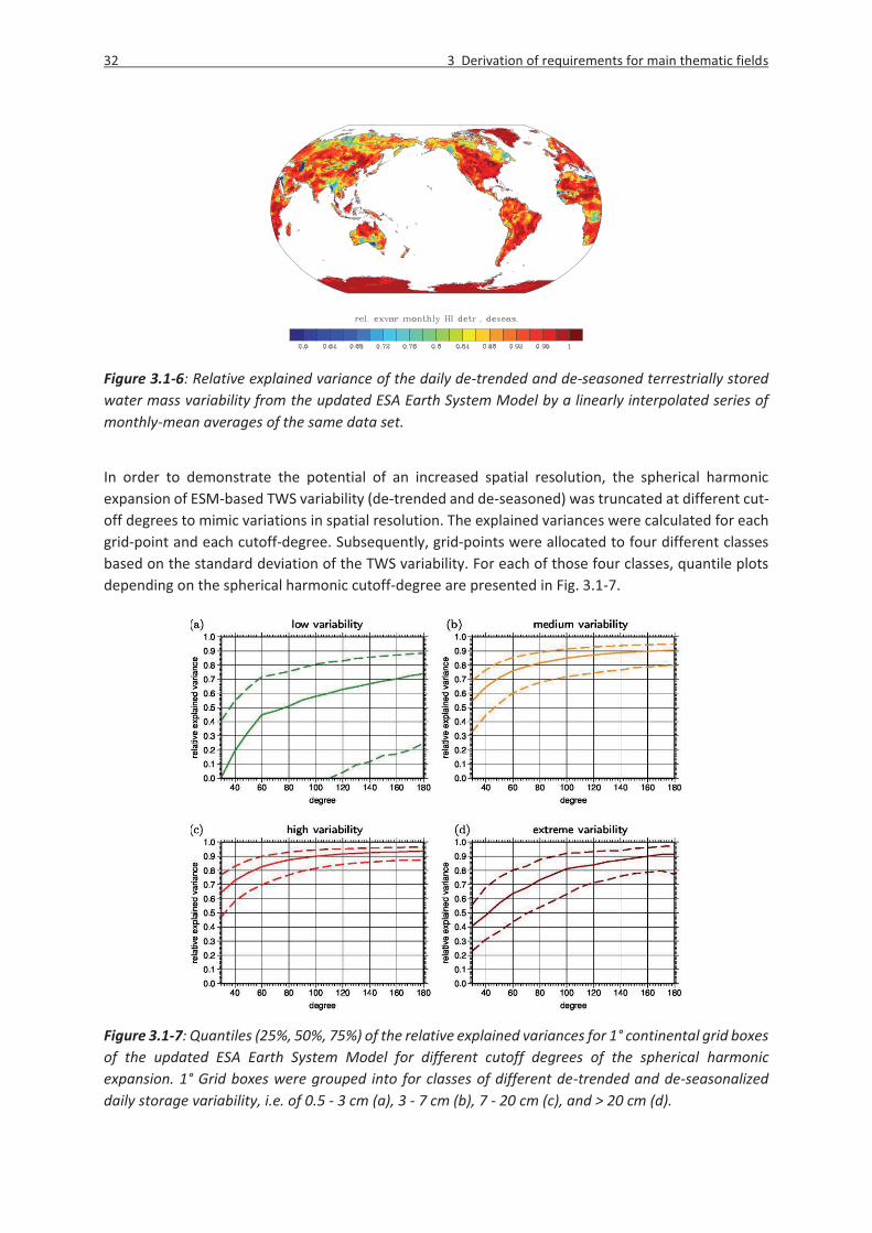
32 3 Derivation of requirements for main thematic fields
Figure 3.1-6: Relative explained variance of the daily de-trended and de-seasoned terrestrially stored water mass variability from the updated ESA Earth System Model by a linearly interpolated series of monthly-mean averages of the same data set.
In order to demonstrate the potential of an increased spatial resolution, the spherical harmonic expansion of ESM-based TWS variability (de-trended and de-seasoned) was truncated at different cut-off degrees to mimic variations in spatial resolution. The explained variances were calculated for each grid-point and each cutoff-degree. Subsequently, grid-points were allocated to four different classes based on the standard deviation of the TWS variability. For each of those four classes, quantile plots depending on the spherical harmonic cutoff-degree are presented in Fig. 3.1-7.
Figure 3.1-7: Quantiles (25%, 50%, 75%) of the relative explained variances for 1° continental grid boxes of the updated ESA Earth System Model for different cutoff degrees of the spherical harmonic expansion. 1° Grid boxes were grouped into for classes of different de-trended and de-seasonalized daily storage variability, i.e. of 0.5 - 3 cm (a), 3 - 7 cm (b), 7 - 20 cm (c), and > 20 cm (d).
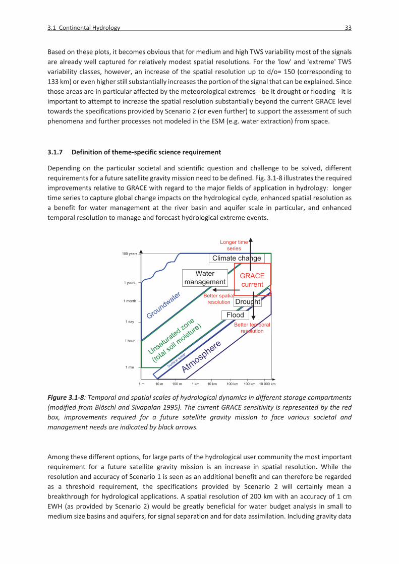
3.1 Continental Hydrology 33
Based on these plots, it becomes obvious that for medium and high TWS variability most of the signals are already well captured for relatively modest spatial resolutions. For the 'low' and 'extreme' TWS variability classes, however, an increase of the spatial resolution up to d/o= 150 (corresponding to 133 km) or even higher still substantially increases the portion of the signal that can be explained. Since those areas are in particular affected by the meteorological extremes - be it drought or flooding - it is important to attempt to increase the spatial resolution substantially beyond the current GRACE level towards the specifications provided by Scenario 2 (or even further) to support the assessment of such phenomena and further processes not modeled in the ESM (e.g. water extraction) from space. 3.1.7 Definition of theme-specific science requirement
Depending on the particular societal and scientific question and challenge to be solved, different requirements for a future satellite gravity mission need to be defined. Fig. 3.1-8 illustrates the required improvements relative to GRACE with regard to the major fields of application in hydrology: longer time series to capture global change impacts on the hydrological cycle, enhanced spatial resolution as a benefit for water management at the river basin and aquifer scale in particular, and enhanced temporal resolution to manage and forecast hydrological extreme events.
Figure 3.1-8: Temporal and spatial scales of hydrological dynamics in different storage compartments (modified from Blöschl and Sivapalan 1995). The current GRACE sensitivity is represented by the red box, improvements required for a future satellite gravity mission to face various societal and management needs are indicated by black arrows. Among these different options, for large parts of the hydrological user community the most important requirement for a future satellite gravity mission is an increase in spatial resolution. While the resolution and accuracy of Scenario 1 is seen as an additional benefit and can therefore be regarded as a threshold requirement, the specifications provided by Scenario 2 will certainly mean a breakthrough for hydrological applications. A spatial resolution of 200 km with an accuracy of 1 cm EWH (as provided by Scenario 2) would be greatly beneficial for water budget analysis in small to medium size basins and aquifers, for signal separation and for data assimilation. Including gravity data
Atmosphere
Unsaturated zone
(total so
il moistu
re)
GRACEcurrent
Longer timeseries
Better spatialresolution
Better temporalresolution
Groundwater
100 years
1 years
1 month
1 day
1 hour
1 min
1 m 10 m 100 m 1 km 10 km 100 km 100 km 10 000 km
Surface water
Flood
Drought
Watermanagement
Climate change

34 3 Derivation of requirements for main thematic fields
of such a high quality will significantly enhance the predictive capability of hydrological models, both on seasonal time scales and for inter-annual variations. For the study of long-term effects and the separation of climatic from anthropogenic drivers a time series length of at least 30 years is required. These long timeseries provided with a trend accuracy of 1 mm/yr on scales of 200 km (as envisaged by Scenario 2) will be sufficient to provide reliable estimates of groundwater depletion and the effects of permafrost thawing and glacier melt on the regional scale and, as a novel application, to distinguish the effect of land use change on water storage from other anthropogenically induced climate change impacts and from natural climate variability. Even though temporal resolution is considered less important (compared to spatial resolution) by large parts of the user community, there is nevertheless considerable interest in near real-time applicability of gravity data with a temporal resolution of a few days and/or a reduced latency of a few days. Therefore, it can be summarized, that in order to meet the societal challenges identified in Section 3.1.1, the following threshold and target requirements can be identified for hydrological applications: Water management: Improved spatial resolution is a clear necessity to work at the scale of river basin and aquifer management.
� Threshold: Scenario 1 � Target: Scenario 2 � Wishful thinking: 1 cm@50 km
Early warning for risk management of extreme events: While spatial resolution is important, low latency data would allow for contributing to near-real time operational forecasting systems. Daily to weekly data is also vital for short-term predictions.
� Threshold: Scenario 1 / Scenario 3, latency of a few days � Target: Scenario 2 / Scenario 4, latency of a few days
Understanding global change impacts on the water cycle: To analyze long-term effects of climate change and to separate natural from anthropogenically driven changes, the most important aspect is a continuous time series in combination with an increased spatial resolution.
� Threshold: extended time series � Target: Scenario 1 � Wishful thinking: satellite gravity as sustained observation infrastructure
35
3.2 Cryosphere 3.2.1 Societal challenges related to the cryosphere
The cryosphere comprises all occurrences on Earth of water in its solid form. The existence of ice on land and in the ocean, its formation and extinction are key elements of global and regional climate processes and exhibit complex interactions with climate change. For example, the high radiation reflectance of snow- and ice-covered areas regulates the Earth’s radiation budget. Melting, freezing and sublimation impacts the atmospheric heat budget. Sea ice formation is a driver of the oceanic thermohaline circulation. The paramount societal challenge of understanding and predicting the climate system and its anthropogenic changes is therefore intrinsically tied to a better understanding of the large variety of cryospheric processes.
Continental ice mass changes directly induce global and regional sea level change. Its understanding and prediction is of utmost societal importance, since large parts of mankind live near the shores. Ice sheets bear the potential of rising sea level by several meters in the coming centuries. The amplitudes of sea level change, as well as the related societal and economic vulnerability, vary geographically and need to be understood based on an understanding of the triggering ice mass change processes.
High societal relevance also arises where glaciers directly control regional hydrological systems through water retention as ice and subsequent melt. Monitoring, understanding, and predicting of their impacts on human water supply are a challenge. They are also needed for emergency management in cases of hazards such as glacially induced flooding.
3.2.2 Scientific questions and challenges and their relation to gravity field signals
While continental snow cover and permafrost are a subject of continental hydrology (Section 3.1), sea ice processes have no direct link to mass distribution and thereby the gravity field. This section therefore focuses on continental ice cover. Following the IPCC terminology, we distinguish between ice sheets and glaciers. Glaciers include mountain glaciers and ice caps as well as the glaciers in the periphery of ice sheets.
The past, present, and future changes of ice sheets (Greenland and Antarctica) is principally determined by the budget between surface mass balance (SMB, i.e. surface accumulation minus ablation) and mass loss due to ice flow. A recent (last 20 years) accelerated decline in mass balance for both ice sheets has been noted (Vaughan et al. 2013 and references reviewed therein, Church et al. 2013, Hanna et al. 2013). These ice losses are linked to polar amplification of global warming, superimposed with possible shifts in large-scale atmospheric circulation pattern, and enhanced by regional positive feedbacks between the ice, atmosphere and ocean. While this mass loss is likely to increase further, not all forcings and feedbacks are sufficiently understood.
In Greenland, current mass loss is approximately equally through SMB (surface meltwater runoff) and enhanced ice flow across the grounding line (van den Broeke et al. 2009). Both atmosphere and ocean have been identified in driving the mass losses. For example, the 2012 record surface melt event in Greenland was mainly forced by the atmosphere (Hanna et al. 2014b), whereas the flow velocities of many tidewater glacier changes are strongly influenced by oceanic forcing (Murray et al. 2010). An emerging field of research and great scientific challenge lies in the connection between surface-melting and ice-dynamics. For the Antarctic Ice Sheets the effect of increased ice flow is dominant. It is triggered by increased basal melt of ice shelves due to warming oceanic boundary conditions forced

36 3 Derivation of requirements for main thematic fields
by changing wind pattern, but also connected to large-scale oceanic transport variations (Pritchard et al. 2012). There is strong interannual variability (Horwath et al. 2012), primarily in the mass gain by snowfall, which has been linked to global atmospheric circulation patterns, such as ENSO (Sasgen et al. 2010, Boening et al. 2012). Increased SMB (snowfall) has at least temporarily increased regional mass balance in East Antarctica (Shepherd et al. 2012, Lenaerts et al. 2013).
The current understanding of mass balance processes is insufficient to predict the near-future evolution of the ice sheets, and consequently sea-level rise. In particular, there is lack of knowledge on the dynamic response of ice flow to changing oceanic and atmospheric boundary conditions, including interactions with intra- and subglacial hydrology. Where the ice sheet is grounded below sea level and deepening inland (like in most parts of the West Antarctic Ice Sheets) positive feedback mechanisms might even lead to ice sheet collapse (e.g. Joughin and Alley 2011). The current lack of understanding the physical processes has prevented the Intergovernmental Panel on Climate Change (IPCC) to include related sea level contributions in their Fifth Assessment Report, thus leaving ice sheet dynamics as a major source of uncertainty to sea level projections.
The past, present, and future changes of glaciers (that is, mountain glaciers and ice caps) poses another set of scientific questions and challenges. In their entirety, glaciers have dominated the eustatic contribution to sea level rise in the last decades, yet the uncertainty of this contribution is even larger than for the two ice sheets, due to the difficulties of extrapolating the sparse sample of observations to the approximately 170,000 glaciers on Earth (Vaughan et al. 2013, Gardner et al. 2013).
Much of the mass losses from mountain glaciers and ice caps are from subpolar climates and maritime coastal environments. These glaciated regions are particularly sensitive to climate variations and are more likely to experience rapid mass losses. For example, the Gulf of Alaska maritime glaciers experienced a significant summer balance season mass loss of approximately 530 Gt in a few months during the 2004 season due to record high summer temperatures in the region (Luthcke et al. 2008) (Figure 3.2-3). The low elevation maritime Yakutat, Glacier Bay and Juneau Icefield regions had the largest negative summer net balance. The Gulf of Alaska glacier mass balance anomalies give a clear illustration of the susceptibility of the subpolar glaciers and ice caps to climate variations and sudden events. In order to fully characterize these events and to model and understand their regional and global impact on life we need a much more comprehensive observational basis.
Ultimately, modeling is the approach to a full understanding and robust prediction capability of ice sheet and glacier changes. Observations are crucial in this context to validate model developments, provide boundary conditions and allow model initialization. Currently, the ability of models to describe recent changes is limited - not to speak about predictions. Therefore, observations are the primary source for describing present-day ice mass changes. Understanding the processes revealed by observations must drive the further development of models with the aim of reaching predicting capability. Various types of observations have illuminated current processes of ice sheet change, including observations of ice surface geometry and its temporal changes by satellite and airborne altimetry, observations of ice flow velocity and its temporal changes by satellite remote sensing, glaciological observations of ice thickness and surface mass balance.
Since continental ice mass changes (and the accompanying changes in the global water mass distribution) inevitably affect the gravity field, observations of temporal gravity field variations provide complementary, integrative information. Indeed, gravity is unique in its direct link to mass changes. Gravity avoids issues of incomplete sampling (present in geometric techniques like altimetry), the restriction to measurements of the top layer of snow and ice, and the ambiguity in converting ice volume change to ice mass change. Gravity also circumvents problems associated with mass budget
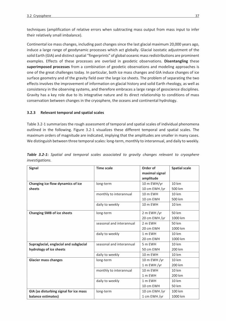
3.2 Cryosphere 37
techniques (amplification of relative errors when subtracting mass output from mass input to infer their relatively small imbalance).
Continental ice mass changes, including past changes since the last glacial maximum 20,000 years ago, induce a large range of geodynamic processes which act globally. Glacial isostatic adjustment of the solid Earth (GIA) and distinct spatial “fingerprints” of global oceanic mass redistributions are prominent examples. Effects of these processes are overlaid in geodetic observations. Disentangling these superimposed processes from a combination of geodetic observations and modeling approaches is one of the great challenges today. In particular, both ice mass changes and GIA induce changes of ice surface geometry and of the gravity field over the large ice sheets. The problem of separating the two effects involves the improvement of information on glacial history and solid Earth rheology, as well as consistency in the observing systems, and therefore embraces a large range of geoscience disciplines. Gravity has a key role due to its integrative nature and its direct relationship to conditions of mass conservation between changes in the cryosphere, the oceans and continental hydrology. 3.2.3 Relevant temporal and spatial scales Table 3.2-1 summarizes the rough assessment of temporal and spatial scales of individual phenomena outlined in the following. Figure 3.2-1 visualizes these different temporal and spatial scales. The maximum orders of magnitude are indicated, implying that the amplitudes are smaller in many cases. We distinguish between three temporal scales: long-term, monthly to interannual, and daily to weekly.
Table 3.2-1: Spatial and temporal scales associated to gravity changes relevant to cryosphere investigations.
Signal Time scale Order of maximal signal amplitude
Spatial scale
Changing ice flow dynamics of ice sheets
long-term 10 m EWH/yr 10 cm EWH /yr
10 km 500 km
monthly to interannual
10 m EWH 10 cm EWH
10 km 500 km
daily to weekly 10 m EWH 10 km
Changing SMB of ice sheets long-term 2 m EWH /yr 20 cm EWH /yr
50 km 1000 km
seasonal and interannual 2 m EWH 20 cm EWH
50 km 1000 km
daily to weekly 1 m EWH 20 cm EWH
10 km 1000 km
Supraglacial, englacial and subglacial hydrology of ice sheets
seasonal and interannual 5 m EWH 50 cm EWH
10 km 200 km
daily to weekly 10 m EWH 10 km Glacier mass changes
long-term 10 m EWH /yr 1 m EWH /yr
10 km 200 km
monthly to interannual
10 m EWH 1 m EWH
10 km 200 km
daily to weekly 1 m EWH 10 cm EWH
10 km 50 km
GIA (as disturbing signal for ice mass balance estimates)
long-term 10 cm EWH /yr 1 cm EWH /yr
100 km 1000 km

38 3 Derivation of requirements for main thematic fields
Changing ice flow dynamics of ice sheets
Changes in ice flow velocity may be induced by changes of either the driving forces or the forces that resist the flow. Driving forces may change on a long term, e.g. due to changing ice thickness or surface slope. Examples for changes in the resisting forces are changes in buttressing stresses by ice shelves induced by ice shelf thinning; changes in basal stresses by changes in subglacial water content, by ungrounding of ice (grounding line migration), or change in the thermal regime and rheology of the ice.
These changes may occur on very different temporal scales. Long-term changes of ice flow may be overlaid by episodic or rapid changes (in days), for example in the sequence of iceberg calving or even ice shelf disintegration, glacier surge events, or events subglacial water intrusion and channeling. The variety in temporal scales poses critical limitations on extrapolating observations beyond the observation interval and to resolve, from a decadal observation series, accurate long-term trends. The ongoing discussion on the nature of the observed possible acceleration of mass loss rates in Greenland and Antarctica (Velicogna 2009; Wouters et al. 2013) arises from these critical limitations.
Concerning the spatial patterns, ice mass changes induced by changes in flow dynamics inherit the complex spatial structure of ice flow (cf. Figure 3.2-2). That is, they are mainly concentrated on narrow outlet glaciers and ice streams.
Changing SMB of ice sheets
Positive SMB anomalies are driven by synoptic precipitation events, affecting areas with a size of hundreds of kilometers on timescales of just days. The typical surface patterns have smaller scales, down to kilometers, and are associated with orographic (lifting and precipitation shadow) and drifting snow effects. Because of the dominance of forced convection in the Polar Regions, even low (on the order of 100 m) and small (on the order of 10 km) topographic disturbances, such as ice rises on ice shelves, may introduce strong snowfall gradients (Lenaerts et al. 2014). Snowfall-induced temporal mass variability is largest in the regions with high precipitation rates, i.e. in the coastal regions, especially upwind of topographical disturbances. Negative SMB anomalies are associated with enhanced meltwater runoff and sublimation. Being both driven in first order by temperature, these patterns are spatially relatively smooth, yet with strong gradients due to the surface topography, concentrating melt production in the narrow ablations zone along the ice sheet margin. Additionally, once melt has started, strong spatial and temporal variability may be introduced here also, for instance by the feedback with albedo, which is a major control on ice melt. Due to this positive feedback, sudden increases in ice melt are possible, as was demonstrated in the exceptionally warm summer over west Greenland in 2012, where infrastructure dating from the 1950's was destroyed by a meltwater-driven flooding event that lasted only 2-3 days.
The large range of temporal scales involved poses critical limitations on the use of observational time series shorter than a multi-decadal climate scale. For example, the question whether recent positive Antarctic accumulation anomalies are already a signal of climate change (Lenaerts et al. 2013) prompts for longer observational time series. They are the only way to resolve long-term trends in the presence of climate variability as well as to study the climate variability by itself, for valuable insights into climate processes.
Glacial hydrology of ice sheets
Processes related to liquid water at the surface, in the interior, and at the bottom of an ice sheet are both extraordinarily complex and essential for the ice sheet regime as a whole. Surface melt water, once it has formed, may locally refreeze in the cold snow/firn, run off over the ice sheet surface, after

3.2 Cryosphere 39
some time penetrate to the bottom of the ice sheet through vertical channels (moulins) or crevasses, become trapped temporarily in supra-, sub- or proglacial lakes. Once it leaves the glacial system, the meltwater may flow into fjords where it interacts with the fjord circulation and enhance frontal melt, or influence the boundary currents in the ocean. Sub-glacial lakes cover up to 5 % of the surface of the grounded part of the Antarctic ice sheet and are an important component of the sub-glacial melting system, influencing basal properties and channeling of ice flow. Our current knowledge about the size and distribution of the active lakes is at best patchy; their interconnections through the sub-glacial drainage system and their episodic discharge events is understood even more poorly. Recently, altimetry observations recorded subsidence of the ice sheet surface of several meters, attributed to a lake drainage event (Mc Millan et al. 2013) with an associated water redistribution of several cubic kilometers over the course of a few months.
Glacier mass changes
Mountain glaciers and ice caps extend at spatial scales from sub-kilometer to hundreds of kilometers, and mass changes occur at all these scales, with a range of amplitudes similar to the one for ice sheet outlet glaciers. Changes in surface mass balance are the major driver of these changes, as many of these ice bodies are land-terminating. As a result, the same challenges as described above for ice sheets apply to these glaciers, albeit at an even smaller scale.
Glacier changes include events of rapid changes. An example is given by the 2009 extreme imbalance of Alaskan glaciers (approximately -140 Gt, that is 50% of the Greenland Ice Sheet mean annual mass balance) (Figure 3.2-3; Luthcke et al. 2013). It was triggered by the eruption of Mt. Redoubt (Arendt et al. 2013) resulting in widespread dark ash covering large portions of the glaciated region and leading to an abnormally low albedo and increased solar energy absorption.
GIA
The viscous reaction of the Earth mantle to ice load changes usually lasts thousands of years. Over the period of satellite observations, GIA is therefore usually considered as linear in time. It is noteworthy, however, that recent attention has been drawn to lateral variations of Earth rheology parameters including low viscosity zones where isostatic compensation of ice load changes may happen on the order of decades (Nield et al. 2014). Long observational time series are favourable to isolate the long-term GIA signal from other, superimposed geophysical signals and from observation noise. Due to the rigidity of the crust between the ice load and the mantle, GIA deformation patterns are spatially more extended and smoother than the original patterns of ice load changes. Solid Earth mass displacements by GIA affect the gravity field, just as ice mass changes do. We express this gravity field effect in terms of equivalent changes of a surface water layer [m EWH], in order to be compatible with the expression of ice mass effects.
The “bubble plots” in Fig. 3.2-1 illustrate the spatial scales and magnitudes of cryospheric signals for different time scales (long-term, monthly to interannual, daily to weekly), and show the accuracy levels assumed for the different mission scenarios.
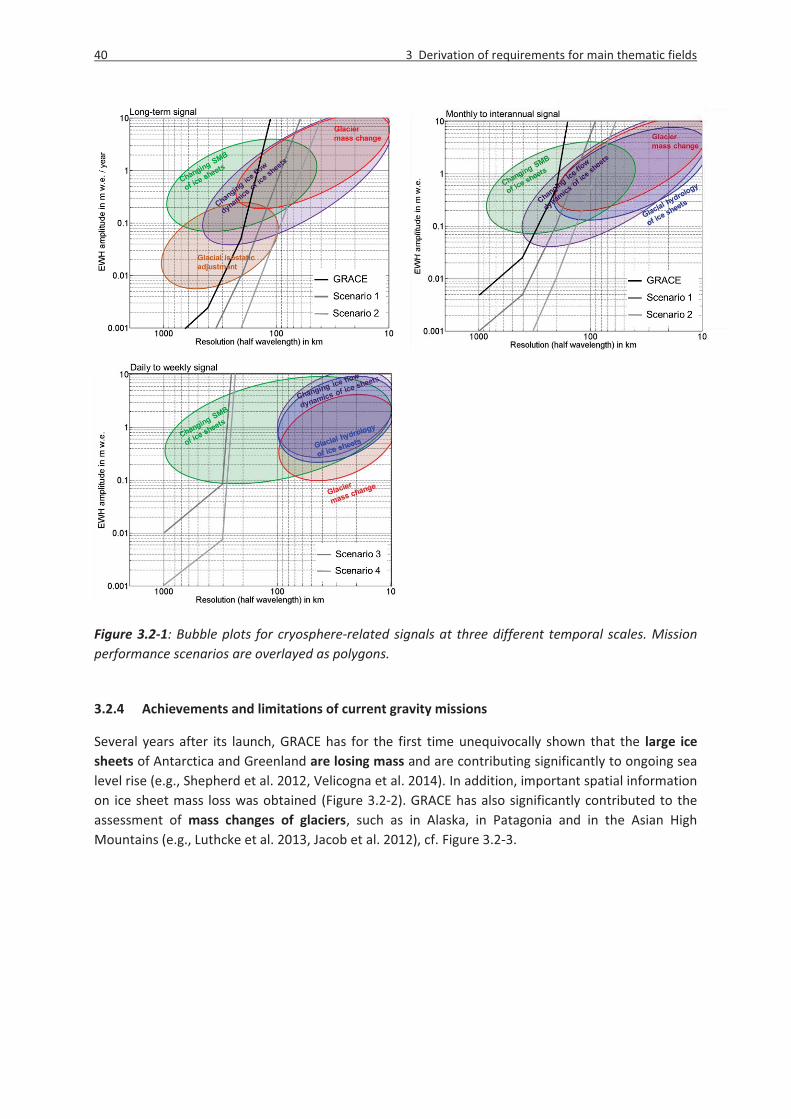
40 3 Derivation of requirements for main thematic fields
Figure 3.2-1: Bubble plots for cryosphere-related signals at three different temporal scales. Mission performance scenarios are overlayed as polygons.
3.2.4 Achievements and limitations of current gravity missions
Several years after its launch, GRACE has for the first time unequivocally shown that the large ice sheets of Antarctica and Greenland are losing mass and are contributing significantly to ongoing sea level rise (e.g., Shepherd et al. 2012, Velicogna et al. 2014). In addition, important spatial information on ice sheet mass loss was obtained (Figure 3.2-2). GRACE has also significantly contributed to the assessment of mass changes of glaciers, such as in Alaska, in Patagonia and in the Asian High Mountains (e.g., Luthcke et al. 2013, Jacob et al. 2012), cf. Figure 3.2-3.
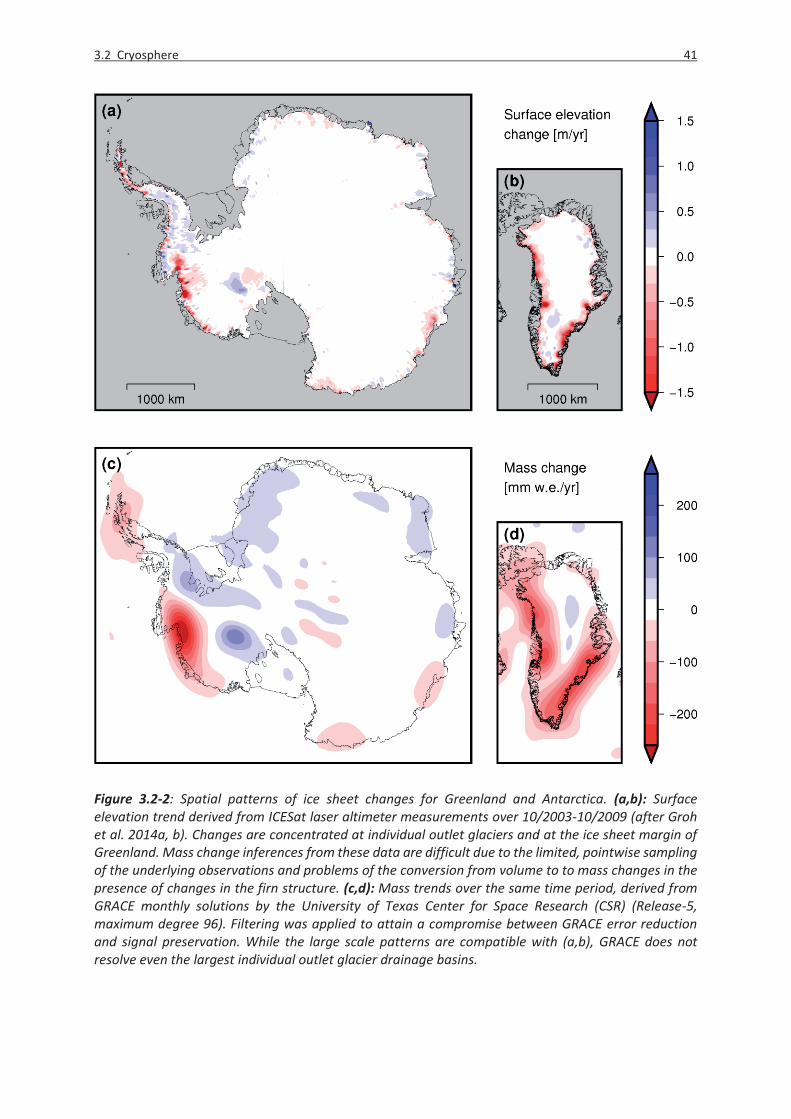
3.2 Cryosphere 41
Figure 3.2-2: Spatial patterns of ice sheet changes for Greenland and Antarctica. (a,b): Surface elevation trend derived from ICESat laser altimeter measurements over 10/2003-10/2009 (after Groh et al. 2014a, b). Changes are concentrated at individual outlet glaciers and at the ice sheet margin of Greenland. Mass change inferences from these data are difficult due to the limited, pointwise sampling of the underlying observations and problems of the conversion from volume to to mass changes in the presence of changes in the firn structure. (c,d): Mass trends over the same time period, derived from GRACE monthly solutions by the University of Texas Center for Space Research (CSR) (Release-5, maximum degree 96). Filtering was applied to attain a compromise between GRACE error reduction and signal preservation. While the large scale patterns are compatible with (a,b), GRACE does not resolve even the largest individual outlet glacier drainage basins.

42 3 Derivation of requirements for main thematic fields
Figure 3.2-3: Mass changes of the Gulf of Alaska glaciers derived from a global mascon solution (Luthcke et al. 2013). (a) Time series of mass changes. (b) annual mass balances. (c) annual changes of individual. Spatial correlations constraints were applied since the individual 1° x 1° mascons could not be resolved otherwise by GRACE. A true 1°-2° mascon resolution would be needed to properly understand the impact of significant climatic changes and their forcings. The figure also shows the strong spatial and temporal variability observed in the lower latitude maritime glacier regions.
More recently, comparisons of ice sheet mass balance results from GRACE with results from the geometric (altimetry) approach and the input-output approach have shown agreement between the complementary methods, within their error bounds. By its direct link to mass changes, GRACE satellite gravimetry has acted as the ultimate independent evaluation tool for the complementary methods (Figure 3.2-4).
Importantly, the continuous GRACE observations with about a monthly temporal resolution have enabled to resolve, and clarify, the temporal variations in the rates of mass change. Such variations were linked to both accelerating ice flow and SMB variations or SMB trends (Rignot et al. 2011, Shepherd et al. 2012, Sasgen et al. 2012, Velicogna et al. 2014, Horwath et al. 2012). Indeed, GRACE has become the primary validation source for modeled temporal variations of SMB (Figure 3.2-4). The new temporal resolution capabilities have lead to a paradigm change from the mere consideration of secular trends to a consideration of signals at a large range of temporal scales. For example, Luthcke et al. (2013) proposed an Ensemble Empirical Mode Decomposition (EEMD) applied to a high resolution mascon solution for quantifying dominant modes in order to identify underlying processes (Gulf of Alaska glaciers annual mass balance shown in Figure 3.2-3).

3.2 Cryosphere 43
Figure 3.2-4: Individual mass balance components of the Greenland ice sheet based on the RACMO2 regional atmospheric climate model and remote sensing of ice discharge, their summed effect (gray) and GRACE results (black). GRACE validates the integral mass balance from the input-output method for Greenland. Figure from Masson-Delmotte et al. (2012). GRACE results courtesy of I. Velicogna and J. Wahr.
There are three major limitations to the mentioned achievements. One limitation is the shortness of the available time series. It significantly impairs the signal-to-noise ratio when attempting to detect and attribute medium-to-long term mass trends in the presence of natural mass variability as well as observation noise (e.g. Wouters et al. 2013). The lengths of present time series are not satisfactory for resolving long-term trends in the presence of climate variability, or for deriving a meaningful reference climatology for models.
As a second limitation, satellite gravity is currently limited to 200-500 km scale (depending on signal strength, time scale and geographic location). Therefore, GRACE only gives coarse, spatially averaged mass signals and is not able to resolve signals down to the spatial scales at which most of the relevant processes occur (Figures 3.2-2, 3.2-5). On the very large scale, uncertainties in long-term trends of the low-degree harmonic components of surface mass change, notably the degree-one and degree-two harmonics, propagate to considerable uncertainties for signals of very large spatial dimension but small amplitude, like in interior East Antarctica.
A third limitation is the inability to separate different superimposed processes of mass redistribution. For vertically superimposed processes (such as GIA and ice mass changes), the absence of separation capability is owing to the physical principles of gravity. For processes adjoining horizontally, the separation limitations are due to the mentioned resolution limits.
Ultimately, all three limitations manifest themselves in different ways as separation problems. Important examples are the following:

44 3 Derivation of requirements for main thematic fields
- Attribution of mass signals to individual glaciers and drainage systems. Since even neighboring
glaciers may have very different climatological/glaciological settings and flow behavior, attributing mass changes to one glacier or another can dramatically change the picture. For example, separating Pine Island Glacier (PIG) mass change from Thwaites Glacier (THW) mass change would be essential since the ice flow regimes are different. PIG has the potential of instability due to its bed geometry.
- Making a clear distinction between mass changes in mountain glacier ice and the surrounding (and probably related) hydrology and possibly related solid Earth processes, such as vertical isostatic motions. Narrowing the glacier mass changes down to individual glaciers or subsets of glaciers situated in climatologically well-defined regions would be ideal, but is a difficult challenge.
- GIA uncertainty. The separation between present-day ice mass changes and GIA-related displacement of solid Earth material is one of the great challenges, owing to the spatial superposition of the two phenomena and large density of the displaced crustal and mantle material, as compared to ice. In fact, GIA is the dominant source of uncertainty for GRACE-based mass balance estimates of the Antarctic Ice Sheet. For example, recent updates of GIA models have significantly affected GRACE-based mass change estimates (King et al. 2012, Ivins et al. 2013). While the incorporation of additional information, from GIA modeling and/or from complementary geodetic observations, is inevitable to overcome this situation, an improved spatial resolution and accuracy of satellite gravity trends would equally benefit these efforts by supporting the distinction of the different spatial characteristics of ice mass changes and GIA.
- Separating ice sheet changes from coastal ocean changes. This task includes the account for the gravitationally consistent ocean changes induced by the ice mass changes themselves, as well as changes due to ocean dynamics (which again, may be linked to continental ice mass changes). Processing steps are likely capable of taking advantage of the spectral character that might be assigned to either the mass changes offshore and the hydrological/cryospheric changes onshore. More work is needed to understand the region-specific spectral character.
The combination with complementary observations is a means of disentangling various mass transport processes. Separating ice mass change and GIA in Antarctica is a prominent example. Various combination approaches have been pursued (Riva et al. 2009; Gunter et al. 2014, Wu et al. 2010, Groh et al. 2012, Gardner et al. 2013), ranging from local to global scale. Involved observables reach from geometry of continental ice to crustal deformation and sea level patterns (absolute or relative) and modelled ice sheet evolution and local vertical motion from precision GPS. The development of such integrative analyses of satellite gravity with complementary observations is just at its beginning. Gravimetry is instrumental in such combinations for the fact that it gives a direct handle on mass conservation and global consistency of mass transport processes. However, currently, the large horizontal resolution gap between satellite gravimetry and the other techniques poses serious limitations on such inversion approaches.
3.2 Cryosphere 45
3.2.5 Identification of potential new satellite gravimetry application fields
The continuation of satellite gravity time series and a higher accuracy of satellite gravimetry will allow monitoring cryospheric ice mass changes on climatic time scales and better separating underlying mass change signals, thereby overcoming present problems in the interpretation of satellite gravimetry.
Unexpected and partly dramatic processes of ice mass change have been going on in the last decades, and this is likely to continue. The availability of satellite gravimetry will be critical for our ability to observe such processes with the aim of understanding and ultimately predicting these processes.
New applications fields are the following:
a) Cryosphere mass balance time series at monthly to multi-decadal time scales to understand climate forcing on ice sheets, glaciers and ice caps
Linking continental ice mass changes to climate changes (including climate forcing on mass balance as well as feedbacks to climate changes) is crucial to understand not only the mass balance mechanisms but the Earth system and climate change as a whole. The links in question cannot be conclusively established before cryospheric mass changes will be comprehensively observed over lengths at climatic time scales (at least three decades). A new satellite gravity mission, continuing and improving upon previous missions, would achieve this major requirement.
Concerning secular trends of the Greenland and Antarctic ice sheets, even the continuation of satellite gravimetry with today’s accuracy would improve the interpretation of changes in terms of climate variability versus climate trend. For instance, the robust identification of a sustained acceleration of ice sheet mass losses needs 2-3 decades of observations (Wouters et al. 2013). Sub-annual sampling (e.g., monthly) is required for the understanding of mass fluctuations and their link to climate.
b) Cryosphere contribution to global and regional sea level
Understanding sea level changes, including the precise closure of the sea level budget and the comprehension of regional patterns of sea level change, needs precise observations of the eustatic contribution from continental ice shrinkage and its geographic origin. A new mission with the target requirement sufficient to include regional glacier mass balance and regionalized ice sheet mass balance will ensure such observational data.
c) Observe and separate GIA as a prerequisite to understand feedbacks between ice mass change and regional sea level
GIA is presently the crucial error source for Antarctic ice mass balance estimates from satellite gravimetry and an essential error source for other glaciated regions. As a prerequisite for applications a) and b), GIA needs to be quantified much more accurately than today. Moreover, understanding GIA is a prerequisite to understand feedbacks between ice mass changes and regional sea level. A major step forward can be achieved by the continuation of satellite gravimetry in a new mission with enhanced accuracy. Both the greater length of the time series and the better performance of the new mission will allow to infer linear trends more accurately and at higher spatial resolution than today. This will facilitate the separation of ice mass, ocean mass, and GIA signals based on their specific fingerprints in the gravity field trends and on enhanced possibilities of combinations with complementary approaches.

46 3 Derivation of requirements for main thematic fields
d) Aid ice sheet modeling and prediction by the determination of mass changes of individual ice sheet drainage basins
Individual glaciers can react very differently to changes in their boundary conditions, for instance due to their different bed geometries. Understanding the reaction of an ice sheet to climate forcing must therefore build on understanding the dynamics on a drainage system level. In order to be a useful data source for constraining and validating respective models, satellite gravimetry must deliver mass change estimates for individual basins, independently of a-priori information. This requires an enhanced spatial resolution as compared to GRACE (cf. Figures 3.2-2, 3.2-5). An enhanced spatial resolution would also enable to separate (through their spatial signatures) dynamically induced changes from SMB-induced changes. Consequently, satellite gravimetry would become an independent, unequivocal data source for dynamically induced changes, not restricted to the episodic temporal sampling inherent to ice flow velocity observations from remote sensing.
e) Aid ice dynamic modeling by observing processes leading to changes in ice flow, including grounding line migration and glacial hydrology
Processes that trigger changes in ice flow dynamics are often even more spatially confined than the ice dynamic changes themselves. The triggering processes include grounding line migration and the whole spectrum of subglacial and supraglacial hydrology. Fundamentally new applications would arise from a mission that brings at least some of the triggering processes into the realm of observability.
A strong enhancement of resolution would also enable the distinction between SMB variation patterns and ice dynamic mass change patterns. Given a sufficient temporal and spatial resolution, satellite gravimetry could indicate the origin of mass changes to be either SMB or ice dynamics or could reveal the links between SMB and ice dynamics, e.g. through glacial hydrology. By imposing leads and lags to optimize correlation of GRACE signals with SMB modelling results, inferences can probably be made about the volume of englacial/supraglacial meltwater storage (see e.g., van Angelen et al. 2013). A better resolution would indeed bring the detection of individual drainage events within reach.
f) Aid atmospheric modeling by observing processes related to SMB changes
Quantifying the contribution to glacier mass balance made by surface processes requires resolving mass changes at daily to decadal time scales. At those time scales the impact of the strong daily cycle of meltwater runoff as well as the role of decadal climate oscillations on glacier surface mass balance become apparent. Although atmospheric models have proven to be capable to model with some accuracy the surface mass balance processes over the large ice sheets of Greenland and Antarctica, they still relatively poorly represent several important mass redistribution processes, such as drifting snow (sublimation and transport), horizontal and vertical water flow in firn, as well as physical and biological surface processes that govern the all-important melt-albedo feedback.
Direct gravity measurements with improved temporal and spatial resolution will thus be invaluable as independent, ultimate evaluation of coupled atmospheric/surface mass balance/firn models. The enhanced resolution will mitigate the present ambiguity of isolating SMB effects from the overall ice mass changes.
g) Determination of mass changes of glaciers
While satellite gravity has proven useful for the determination of mass changes of mountain glaciers and ice caps, results from GRACE cannot distinguish between glaciers within regions of several hundred kilometers dimension. Moreover, the ambiguity between ice masses and hydrological water storage on the surrounding land areas is a considerable concern.
3.2 Cryosphere 47
An improved spatial resolution and accuracy will largely reduce these limitations. As a new application, satellite gravity will serve as a truly comprehensive and unequivocal source of the mass balance of glaciers with at least monthly resolution and global coverage – something absolutely unaffordable by classical glaciological observations. Even if satellite gravimetry will not resolve individual glaciers, the reliable mass balance for clusters of glaciers at 100-150 km dimensions will place glaciological monitoring and modeling on an unprecedented data basis (cf. Figure 3.2-3).
h) Observation of glacier processes for hydrological and emergency applications (flooding, water storage, hydro power)
As an ambitious operational application, glacier mass change observations on high spatial resolution (ca. 25 km) and small temporal latency (days) could serve applications in water management and emergency management. Examples are the management of water supply for settlements, industry and hydropower plants, and the emergency management for cases of episodic or catastrophic events, such as meltwater flooding or processes induced by ash cover following volcanic eruptions.
i) Technique combination
Beyond the isolated use of satellite gravimetry, an enhanced resolution of gravimetry will boost the success of technique combinations for the separation of processes. Once gravity information is available in an enlarged spectral range, the corresponding spectral range in complementary datasets, e.g. satellite altimetry, can be exploited in combination approaches. This will provide discriminatory information, e.g., for the discrimination of dynamically induced ice mass changes (spatially correlated to places with large ice flow), GIA (much smoother, and therefore more extended in space), and descent or ascent of interannual precipitation.
3.2.6 Added value of individual mission scenarios
The most basic need, and therefore the first priority, of the cryospheric user community consists in the continuation of satellite gravity missions to reach the climatic time scales that are a demand for applications like the derivation of cryosphere mass balance time series at monthly to multi-decadal time scales to understand climate forcing on ice sheets, glaciers and ice caps (a) and the cryosphere contribution to global and regional sea level (b), and a strong benefit for all other applications. As the second priority, a new mission should have improved spatial resolution, or equivalently, less noise at small spatial scales. The third priority is an increased temporal resolution.
The increase in spatial resolution offered by Scenario 1 would allow to realize a number of new applications listed in Section 3.2.5. Therefore, this Scenario would mean an essential step forward for cryospheric sciences. The leap in accuracy offered by Scenario 2, as compared to Scenario 1, would be a breakthrough for applications like the separation of GIA effects (c), the determination of mass changes of glaciers (g), and technique combinations for the separation of the processes (i). In many cases, the degree to which applications can be realized depends gradually on the mission performance. Therefore, naturally, Scenario 2 would be an essential additional benefit to those applications that may be already addressed by Scenario 1. It is worth mentioning that a satellite gravity mission involving near-polar orbiting satellites provides a better accuracy in polar regions than on a global average (e.g., better by a factor of two for GRACE). Finally, wishful thinking performances well beyond the specified scenarios are required for tasks like the observation of glacier and ice cap processes for hydrology and emergency applications (h) as well as for smaller-scale realisations from the other application fields. In the following, a few examples are elaborated for the above statements.

48 3 Derivation of requirements for main thematic fields
Concerning the separation of ice sheet drainage basins (application d), the glaciers in the Amundsen Sea Sector (Pine Island Glacier; Thwaites Glacier; and Haynes, Smith and Kohler Glacier system; see Figure 3.2-5a) are an important case. The distance between the glacier trunks is about 150 km. Given the large amplitude of mass changes (on the order of 0.5 m EWH over one year on the 150 km scale), these basins may be separated by Scenario 1, while they cannot be separated by GRACE without the use of external information. Similarly, Scenario 1 will allow to separate the two large glacier complexes in Northeast Greenland, namely the 79° Glacier/Zachariae Glacier complex and the Storstrømmen, which are about 150 km apart. On the other hand, Jacobshavn Isbrae, the Greenland glacier with the most dramatic changes over the past decade, is in a distance of about 80 km from its northern neighbors (e.g., Eqip Sermia) large glaciers, which exhibit remarkable, but different, dynamics. An accuracy better than Scenario 2 is required to allow a separation of the different drainage basin signals at least on a 50 cm EWH/yr accuracy level. In terms of wishful thinking we may think of separating the mass signals at the Eastern and Western side of the Antarctic Peninsula, with very different regimes of SMB and different boundary conditions on ice flow. The distance is 50 km or less. This requirement would need a mission substantially more accurate than Scenario 2.
As an example for the separation of glaciers (application g), distinct glaciated mountain ranges within the Golf of Alaska region are about 150 km apart. GRACE analyses suffer significant signal leakage between those subregions (Arendt et al. 2013). Given annual mass variations on the order of 1 m EWH, Scenario 2 would fully satisfy the need of separation between these mountain ranges and would also significantly aid the distinction between glacier mass changes and hydrological variations on the surrounding ice-free areas. This scenario would therefore mean an enormous benefit. Scenario 1 could still be a compromise but would degrade the monthly accuracy level at 150 km to 50 cm EWH, that is, similar to the expected signal amplitudes.
Glaciers contribute about as much to eustatic sea level rise as the two ice sheets. Therefore, applications a) and b) depend on the requirements for glacier mass balance. Scenario 2 would be appropriate, while Scenario 1 would be a compromise.
Concerning a better separation of GIA from ice mass signals (application c) we may note that Antarctic GIA patterns extend about 200 km into the ocean, with magnitudes of about 10 mm EWH/yr. To separate these patterns unequivocally from ice mass signals leaking out into the ocean, we would need the secular trend with, say, 2mm EWH/yr accuracy at 150 km resolution. Scenario 2 is near to fulfilling these requirements, in view of the expected enhanced accuracy in polar regions.
Applications e) and f) address a multitude of tasks and related requirements. One of the phenomena related to both application fields is glacial hydrology. An event of water discharge of 5 Gt from a subglacial lake (as reported from altimetry by McMillan et al. 2013) over a hypothetic distance of 200 km (cf. Wingham et al. 2006) would constitute a signal of 0.12 m EWH at 200 km scale (5 km3 divided by 200x200 km2). This would be resolvable by Scenario 1. Events with smaller discharge volume or smaller distance of discharge could be resolved by averaging over a number of months before the event and after the event, or by Scenario 2. Therefore, satellite gravimetry could offer an additional means (in addition to satellite altimetry) of monitoring large water mass exchanges in a subglacial hydrological network. In fact, inside the polar gap of altimeter missions (beyond 81.5° or 88°, depending on altimeter mission), satellite gravimetry would be the only way of detecting such events.
To be able to distinguish changes due to SMB from changes due to ice flow dynamics just from their spatial signatures in satellite gravimetry, we would like to have a 0.1 m EWH accuracy at a spatial resolution of 80 km and temporal resolution of 1 yr, leading to a 0.35 m EWH monthly accuracy requirement at 80 km. Even Scenario 2 has an error level ten times larger than that. Therefore, this kind of separation is referred to a wishful thinking.

3.2 Cryosphere 49
Finally, application h) would require at least a 25 km resolution, be it with a 1 m EWH accuracy. This is, again, a wishful thinking scenario.
Figure 3.2-5: Illustration of ice sheet mass change signal content and signal omission for different spatial resolutions. For this simulation, elevation trends shown in Figure 3.2-2 (a,b) are used as a proxy for the spatial patterns and spectral properties of the actual mass change signal. (a) Signal retained by different spatial resolutions for the example of the Amundsen Sea Sector of West Antarctica. PIG, THW and HSK mark the Pine Island Glacier, the Thwaites Glacier and the Haynes/Smith/Kohler glaciers, respectively. (b) Signal omitted due to the respective resolution limits. The sum of (a) and (b) in each column gives the full signal. (c) Evaluation of the omission error, expressed as the ratio between its variance and the variance of the total signal. This calculation is based on the entirety of the Antarctic and Greenland ice sheet change patterns. Annotated circles illustrate how omission errors for a given level of GRACE measurement error reduce with Scenario 2 as compared to GRACE.
50 3 Derivation of requirements for main thematic fields
Figure 3.2-5 illustrates the ice sheet signal content retainable with different spatial resolution. Overall, continental ice mass changes show strong spatial concentration, lending great importance to small spatial scales. While even a 100 km resolution leaves 50% of the variance of the spatial patterns unobserved, an increase in resolution according to the target Scenario 2 would dramatically reduce the signal omission and lend dramatically higher fidelity to the patterns of change derived from satellite gravimetry. 3.2.7 Definition of theme-specific science requirement
In result of the discussion in Sections 3.2.5 and 3.2.6 we may qualify the application-specific requirements as follows.
a) Cryosphere mass balance time series at monthly to multi-decadal time scales to understand climate forcing on ice sheets, glaciers and ice caps
� Threshold: Scenario 1 � Target: Scenario 2
b) Cryosphere contribution to global and regional sea level
� Threshold: Scenario 1 � Target: Scenario 2
c) Observe and separate GIA as a prerequisite to understand feedbacks between ice mass change and regional sea level
� Threshold: Scenario 1 � Target: Scenario 2
d) Aid ice sheet modeling and prediction by the determination of mass changes of individual ice sheet drainage basins
� Threshold: Scenario 1 � Target: Scenario 2 � Wishful thinking: 1 m EWH at 25 km with monthly resolution
e) Aid ice dynamic modeling by observing processes leading to changes in ice flow, including grounding line migration and glacial hydrology
� Wishful thinking: 1 m EWH at 25 km with weekly resolution
f) Aid atmospheric modeling by observing processes related to SMB changes
� Threshold: Scenario 1 � Target: Scenario 2 � Wishful thinking: 1 m EWH at 25 km with weekly resolution
g) Determination of mass changes of glaciers
� Threshold: Scenario 1 � Target: Scenario 2 � Wishful thinking: 1 m EWH at 25 km with weekly resolution

3.2 Cryosphere 51
h) Observation of glacier and ice caps processes for hydrological and emergency applications (flooding, water storage, hydro power)
� Wishful thinking: 1 m EWH at 25 km with weekly resolution
i) Technique combination � Threshold: Scenario 1 � Target: Scenario 2 � Wishful thinking: 1 m EWH at 25 km with monthly resolution
In conclusion, Scenario 2 would really open the major application fields a), b), c), d), f), g) and i). We qualify Scenario 2 as the target requirement. Scenario 1 would allow to realize part of the identified applications and would be still an important step forward with respect to previous satellite gravity missions. We qualify Scenario 1 as the threshold requirement.
Wishful thinking scenarios that push the spatial resolution to about 25 km and the temporal resolution to a few days would be needed for the application fields e) and h). Such scenarios would also, again, revolutionize the benefit from those application fields already addressed with the threshold and target scenarios.
52
3.3 Oceanography 3.3.1 Societal challenges in oceanography
The global ocean plays an important role in many of the problems facing society today. If society is to adapt to and mitigate against these threats, it is crucial that we have the observations that will allow us to monitor, understand and predict oceanographic processes. Among these, observations from satellite gravimetry can provide unique insights into the behaviour of the ocean. Satellite gravimetry is therefore a tool with great potential in helping us address the societal challenges in which the ocean plays a role. With a large fraction of the world’s population living, and major cities built, on land with an elevation less than 1 meter above sea level, rising sea level is one of the most serious consequences of climate change. Sea level is rising globally (presently at a rate of about 3 mm/yr) due to ocean warming, and the consequent steric expansion, and from mass input from melting ice sheets and glaciers (Fig. 3.3-1). Since each of these has its own response to climate change, if we are to make better predictions it is essential that we can distinguish between them. As only satellite gravity offers the possibility to observe mass changes in the oceans, it clearly plays a crucial role in helping us meet the grave societal challenge of rising seas. A related challenge, also of great societal importance, is the ability to understand and predict decadal fluctuations and secular changes in Earth’s global mean surface temperature. Decadal fluctuations obscure, and therefore make it more difficult to predict, the secular, anthropogenic change in climate. Therefore accounting for decadal fluctuations in global temperate is critical in understanding and accurately predicting the human impact on climate, which is necessary if we are to take appropriate action to limit global warming and address its consequences, either through adaption and/or mitigation. Decadal fluctuations are important in their own right too: they are too short to adapt to, but too long to ignore. There is growing evidence that due to its large heat capacity the ocean has a strong influence on decadal fluctuations in global mean temperature, including the recent global warming hiatus. By giving us the ability to discriminate between regional sea level fluctuations due to mass redistribution and those due to oceanic heat up-take, satellite gravity can be used to identify where the ocean is taking up heat and how this is changing over time. This will lead to a better understanding of the role of ocean dynamics in ocean heat uptake and how the ocean affects global surface temperatures on decadal and secular timescales. By carrying relatively warm water from the equator to much cooler northerly latitudes, the Atlantic meridional overturning circulation (AMOC) plays a crucial role in regulating Earth’s climate and maintaining the relatively mild climate of North-western Europe. Evidence from climate models and palaeo records suggest that changes in the AMOC go hand-in-hand with relatively rapid, global-scale changes in Earth’s climate. Elevated levels of freshwater input into the sub-polar North Atlantic – as is currently occurring due to warming-induced melting of the Greenland ice sheet – may cause a slowdown or, in the extreme, a collapse of the AMOC. The potential magnitude of the associated changes in climate, combined with the rapid speed with which they could occur, would be very difficult for society to respond to. It is therefore vital that as the Earth warms the AMOC is carefully monitored over many decades to understand and predict how it is responding, and will respond to, a warming climate and increased freshwater input from the Greenland ice sheet. As will be shown below, a sufficiently accurate satellite gravity mission would potentially enable us to monitor this vital
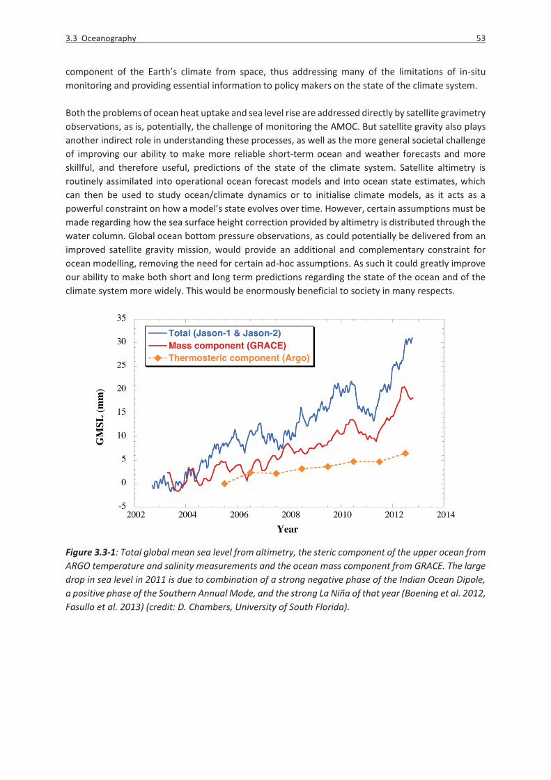
3.3 Oceanography 53
component of the Earth’s climate from space, thus addressing many of the limitations of in-situ monitoring and providing essential information to policy makers on the state of the climate system. Both the problems of ocean heat uptake and sea level rise are addressed directly by satellite gravimetry observations, as is, potentially, the challenge of monitoring the AMOC. But satellite gravity also plays another indirect role in understanding these processes, as well as the more general societal challenge of improving our ability to make more reliable short-term ocean and weather forecasts and more skillful, and therefore useful, predictions of the state of the climate system. Satellite altimetry is routinely assimilated into operational ocean forecast models and into ocean state estimates, which can then be used to study ocean/climate dynamics or to initialise climate models, as it acts as a powerful constraint on how a model’s state evolves over time. However, certain assumptions must be made regarding how the sea surface height correction provided by altimetry is distributed through the water column. Global ocean bottom pressure observations, as could potentially be delivered from an improved satellite gravity mission, would provide an additional and complementary constraint for ocean modelling, removing the need for certain ad-hoc assumptions. As such it could greatly improve our ability to make both short and long term predictions regarding the state of the ocean and of the climate system more widely. This would be enormously beneficial to society in many respects.
Figure 3.3-1: Total global mean sea level from altimetry, the steric component of the upper ocean from ARGO temperature and salinity measurements and the ocean mass component from GRACE. The large drop in sea level in 2011 is due to combination of a strong negative phase of the Indian Ocean Dipole, a positive phase of the Southern Annual Mode, and the strong La Niña of that year (Boening et al. 2012, Fasullo et al. 2013) (credit: D. Chambers, University of South Florida).

54 3 Derivation of requirements for main thematic fields
3.3.2 Scientific questions and challenges and their relation to gravity field signals
As the climate warms over the coming decades, there are many gaps in our understanding of the physical ocean that must be addressed if we are to take the appropriate steps to mitigate or ameliorate the impacts of climate change. Broadly speaking these can be grouped into four categories: Sea level change; The internal dynamics of the ocean; The ocean’s role as a component of the Earth system; The ability to accurately forecast the future state of the climate system. Below we provide an overview of the questions and challenges in each of these areas and the role that satellite gravity can play in answering them. Sea level rise
Rising seas are one of the greatest threats facing humankind over the coming centuries. Satellite altimetry provides an accurate measurement of changes in global mean sea level. Since the early 1990s global mean sea level has been rising at a rate of approximately 3 mm/yr. Sea level rise occurs due to steric expansion (directly related to the density of the sea water, mainly due to changes in the heat content of the ocean, but also to changes in the salinity of the sea water), and, due to the addition of mass to the ocean (e.g., caused by melting of land ice). The ability to discriminate between these two contributions (see Fig. 3.3-1) is crucial in understanding how to Earth system is responding to climate change and to improve our ability to predict how sea level is likely to change in the future. Argo profiling floats can provide estimates of global and regional steric height changes from which, in principle, in combination with satellite altimetry, mass changes can be inferred. Yet, this yields an incomplete picture, since the Argo floats sample only the upper 2000 m of the ocean, introducing a substantial uncertainty related to the steric contribution of the deep ocean. Furthermore they suffer from many limitations common to in-situ observing systems. Their sampling of the ocean is and will remain sparse in both time and space. This entails the use of interpolation methods to provide a global picture. In-situ floats do not provide a measurement platform with stable, consistent and homogeneous error characteristics, such as can be provided by a satellite observing system. It is likely that even with float technology improvements the deep ocean will remain very sparely sampled. Thus, with sufficient space and time resolution, satellite gravimetry is a more suitable tool, in combination with altimetry for estimating global mean and large scale patterns of steric sea level variations. As the only measurement system capable of directly measuring changes in the ocean’s total mass as well as regional mass variations, satellite gravimetry will be an essential tool in understanding the threat posed by rising seas. Although global mean sea level is a useful integrated measure of how the ocean is responding to climate change, it is regional and in particular coastal sea level change that matters to society. There are many factors driving regional and coastal sea level change, including ocean dynamics. Untangling these factors will improve our understanding of the role of ocean dynamics in regional and coastal sea level change and will enable more robust predictions of future coastal sea level change. The ability to separate the mass and steric components of regional sea level as could be provided by satellite altimetry and satellite gravimetry is a powerful diagnostic for understanding the processes that drive regional sea level variations. A gravity mission can also help by better constraining glacial-isostatic adjustment (see Sections 3.2.5, 3.4.2, 3.5), which affects relative sea level at coastal zones through land subsidence. If attainable at a sufficiently high resolution, the ability to discern between regional mass and steric sea level change can be crucial in understanding how the climate system is working, in terms of changes in atmospheric circulation patterns, hydrological cycle, etc., much more than simply looking

3.3 Oceanography 55
at the global mean. The ocean has the capacity to take up, store and release vast quantities of heat. As well as affecting global mean and regional sea level variations, heat fluxes between the atmosphere and the ocean have the potential to modify land and ocean surface temperatures and alter the ocean’s circulation. These impacts and how long the heat may be stored for depend on where the changes in heat content occur. Tracking where this heat is being taken up by the ocean, determining how much is being stored in the deep ocean, and understanding the processes that control this are all important to understand sea level rise and improve the predictive skill of climate models. Additionally, this will provide a step forward in closing the thermal energy balance of the climate system by relating variations in the rate of Earth’s mean temperature to ocean heat content storage. By allowing us to remove the mass component from altimetric sea level we could study heat content changes, and infer changes in the salinity level of the sea water (freshening). Further by combining this with Argo sampling of the upper ocean we could examine steric changes in the deep ocean. Currently, the time series of ocean mass changes from gravimetry spans about 10 years. In the Earth's climate system, naturally forced variations affecting sea level have time-scales of several decennia. To assess how the climate system in general and the sea level in particular will respond to rising levels of CO2 and the potential of natural variations to ameliorate or exacerbate man-made changes we must build up an observational record of sufficient length to discriminate between anthropogenic and naturally forced variations in global and regional sea level. The ability to separate the mass and steric components where the climate sensitivities and range of natural variations is likely to be different will aid the attribution and detection of anthropogenic sea level changes. Internal ocean dynamics
Our understanding of the dynamics of the ocean remains inadequate. Skillful climate forecasts will require improved representation of these processes in ocean/climate models. As already noted, by decoupling the steric and mass components of sea level signals, satellite gravimetry can improve our understanding of ocean dynamics. However, the bottom pressure variations and the time mean dynamic topography that can potentially be provided by a satellite gravity mission are also powerful tools for investigating the ocean’s internal dynamics. Ocean dynamics are essential for estimating basin scale transport of heat and freshwater variations. As an example of this, consider that if we know the bottom pressure variations on the continental slopes of the Atlantic, then we could easier measure the Atlantic meridional overturning circulation (AMOC), which plays a crucial role in the Earth's heat transport. Because such variations are confined to relatively narrow slopes, this would place a tight constrained on the required spatial resolution. So far, gravimetry has not been shown to be capable of detecting variations in the AMOC, but this may change when observations with a higher resolution and reduced noise level become available (Bingham and Hughes 2008, 2009). Furthermore, the capabilities of gravimetry for mapping regional bottom pressure variability allow for better insight on barotropic circulation changes, including depth mean currents, that are very difficult to obtain by other means. The assimilation of bottom pressure data, together with altimetry and other data, into ocean models could improve the determination of the oceanic baroclinic and barotropic circulations. When averaging its observations over a sufficiently long time, satellite gravimetry provides the best option for determining the geoid. If the ocean were at rest, its surface would coincide with the geoid. However, wind and buoyancy (heat and freshwater) force the ocean water to circulate. The geoid may

56 3 Derivation of requirements for main thematic fields
be combined with observations of the mean sea surface height from altimetry to derive the mean dynamic topography (MDT) of the ocean. The mean ocean surface currents are related to the MDT through geostrophy, and provide important information about the currents – such as the Gulf Stream – that redistribute heat and thus regulate the Earth's climate. Furthermore, gravimetry observations with a high spatial resolution (in the order of a few 10 kilometers), along with altimetry, can be used to map the circulation and help understand the role of eddies in the ocean. Eddies play an important role in (vertical and horizontal) mixing and transporting of heat and biochemical materials in the oceans, but due to the lack of observations, their exact role is not well understood. Understanding the ocean as an Earth system component
Our knowledge of many of the large and small-scale processes within the ocean and at its boundaries – crucial for understanding energy balances and the ocean’s large-scale characteristics – remains inadequate. Many large-scale phenomena affecting climate on interannual time-scales – such as the AMOC, ENSO, NAO, AMO, etc. – involve interaction between the atmosphere and the ocean. Yet, the balance of power within these processes is still poorly understood. Understanding this balance of power and how it may shift in a warming climate is an important question for oceanography and climate research. For example, how is the AMOC responding to changing ocean/atmospheric conditions and what will the long term impact of any MOC changes – a slowdown for example – be on the European/global climate system. A better understanding of these processes will be crucial for untangling natural from anthropogenic variability and in making skillful decadal climate forecasts. As mentioned above, combining time-variable gravity observations with altimetry allows the decoupling of mass and steric components. If the spatial resolution of the gravity data can be improved, this may allow tracking of movement of warm water cells towards the polar regions, where the interaction with ice sheets/ice shelves has the potential to induce accelerated ice melt. The response of the cryosphere to warming oceans is paramount in projections of future sea level rise, as it may represent a major contributor. As discussed in Chapter 3.2, GRACE is able to observe the mass changes of the major ice sheets and glaciers, allowing us to directly estimate their contribution to sea level rise. In turn, these gravimetry observations can be used to constrain the freshwater input from the ice sheets in global ocean circulation models. The ability to accurately forecast the future state of the climate system
One of the grand challenges of climate science is to move from climate projections to skillful climate forecasts that will be useful to policy makers for social and economical decision making. This will involve coupled state estimation and optimal use of modelling and observational resources. Although clearly a topic broader than oceanography, the requirement for useful climate forecasts will be an important driver of oceanographic research in the coming decades, and many of the challenges discussed above can be viewed as being in service of this overarching objective. The quality of near-future climate predictions is strongly dependent on how models are initialized: their state at the start of the prediction should resemble reality as close as possible. Satellite gravimetry, together with altimetry and Argo sampled upper ocean, provides the best option for monitoring heat changes in the deep ocean, including deep contributions currently hard to observe with available measurements, and similarly for freshwater storage. Further, satellite gravimetry can contribute by providing estimates of present-day trends in global and regional ocean mass, and its acceleration (provided the time series are adequately long). These observations can serve as input for (semi-)empirical forecasts of future sea level rise.

3.3 Oceanography 57
3.3.3 Relevant temporal and spatial scales
Discrimination between mass and steric components of sea level is the primary benefit of a gravity mission. Essentially this means detecting bottom pressure signals. These cover a wide range of spatial scales and amplitudes, which are discussed below and illustrated in Fig. 3.3-5: Table 3.3-1: Spatial scales and amplitudes of the ocean processes of interest
Signals Time scales Expected signals: temporal variation in equivalent water height
Spatial scale
Mass input (global)
secular 1 mm/yr global interannual 1 mm (with peak-to peak
variations of ~5mm) seasonal 10 mm
Basin scale mass redistributions
secular 1 mm/yr > 10000 km interannual few mm seasonal 5 mm
Regional mass variations
secular ~ 3 mm/yr 0(100-1000) km interannual 5 mm, locally up to 15 mm
seasonal 10 – 50 mm with local peaks up to 20 cm
Boundary processes (incl. MOC)
decadal 1-20 mm 20 – 200 km
Ocean tides hours to years 0-5000 mm 0(100-1000) km GRACE has been used to estimate the long-term trend in ocean mass, which is in the order of ~1 mm/yr (Table 3.3-1). Given the ~10 year time series, the trend estimates are still affected by interannual and decadal variability. In fact, GRACE showed that many interannual variations in global mean sea level (GMSL) corresponds to changes in the mass component and not the thermosteric sea level. In particular, the 5 mm drop in GMSL in 2011 has been linked to excessive precipitation in Australia, which could be attributed to a very unique combination of a strong negative phase of the Indian Ocean Dipole, a positive phase of the Southern Annual Mode, and the strong La Niña of that year (Fasullo et al. 2013). Longer time series are required to come to more robust trend (and acceleration) estimates and to disentangle the effect of climate modes on global and regional sea level. Since the power of these modes generally lies at the decadal time scales, time series with a length of several decades may be required. Also, the results for the global ocean mass trends depend strongly on the models used to correct for glacial isostatic adjustment (GIA). It is expected that longer GRACE time series will lead to improved GIA models, thereby reducing the uncertainty in the ocean mass trend estimates. At the basin-scale scales, the volume of water exchanged between the Atlantic, Pacific and Indian Ocean is in the order of 1000 km3, while interannual variability has been show to amount to 200-400 km3 (Chambers and Willis 2009). Due to the large area of the ocean basins, the associated change in equivalent water height is small (a few mm), yet this signal can still be retrieved by current satellite gravimetry due to its large length-scale.

58 3 Derivation of requirements for main thematic fields
Regionally, seasonal redistribution of ocean water has an associated signal of typically 1 cm or less, with slightly higher values (~5 cm) in regions where wind forcing is significant combined with weakened H/f gradients (H = ocean depth; f = Coriolis parameter), such as the northwestern Pacific and the Southern ocean (Vinogradov et al. 2008). Extreme values of seasonal ocean bottom pressure variations with amplitudes up to 20 cm with length-scales of a few 100 kms have been detected by GRACE in coastal semi-enclosed shelf zones, such as the Gulf of Thailand and the Gulf of Carpentaria (Australia) (Tregoning et al. 2008, Wouters and Chambers 2010). Interannual variability is an order of magnitude smaller (~ 5 mm), with higher values (up to 1.5 cm) found in shallow or semi-enclosed areas such as the Indonesian and Nordic Seas and the aforementioned areas of strong wind stress curl and weakened H/f gradients such as the Australian-Antarctic Basin and the Bellingshausen Basin (Piecuch et al. 2013, Ponte and Piecuch 2014). As discussed in section 3.3.4, little work has been done to evaluate low-frequency variations in the transport of the major ocean currents, however, except for some evaluation of correlations between GRACE derived transport for the Antarctic Circumpolar Current (ACC) averaged over the Pacific sector and the Southern Annual Mode (SAM). Although correlations between GRACE-derived transport and SAM have been shown to be high (Bergmann and Dobslaw 2012), the results are likely biased by the high-frequency and seasonal variability. No analysis was done for the longer than annual period. However, assuming monthly errors of 3 Sv (1 Sverdrup = 106 m3/s) with a random autocorrelation, a change in transport of less than 0.3 Sv/year should be detectable by GRACE with 90% confidence using the current 10-year record. Continued time series will further increase the confidence of the estimates. Even more challenging than assessing the ACC transport, the largest ocean current, is the measurement of surface and deep ocean boundary currents, which have length-scales in the order of 20-200 km, and which often flow along the contours of steep continental slopes (Hughes and Legrand 2005). Examples of particular interest are the Gulf Stream and its deep counterpart the Deep Western Boundary Current. These currents form part of the AMOC, which, by transporting vast quantities of freshwater and heat, plays a central role in regulating Earth’s climate. Bingham and Hughes (2008, 2009) find a bottom pressure signal on the continental shelf of the US east coast of around +2 cm (eq. water height) for each Sverdrup drop in AMOC transport strength, with an opposite change in bottom pressure of -1 cm on the lower continental slope. The relative weakness and O(100 km) length scale of the bottom pressure/geoid changes associated with AMOC variability poses a significant challenge to the ability of satellite gravity missions to detect such signals. In fact, the weaker lower-slope signal [at ~1300-3000 m depth] may be more readily detected given that it is further from the coast and so less affected by leakage from continental hydrology. Clearly, a leap in resolution and accuracy will be required to monitor variations at annual and even inter-annual time scales. However, the variations in the major deep-ocean currents affecting continental climate have periods of a decade or longer, so that a viable solution may be to difference gravimetric observations averaged over 10 year periods (thereby reducing the noise) and infer such low-frequency changes (Hughes and Legrand 2005).
3.3.4 Achievements and limitations of current gravity missions
In the following, the main achievements of gravimetry in oceanography will be discussed.1 Oceanography benefits from both the time-mean and time-variable components of satellite gravity. The mean component (the geoid) can be combined with sea surface height (SSH) from satellite
1 This section is based on the oceanography section in Wouters et al. (2014), written by Don Chambers (University of South Florida).

3.3 Oceanography 59
altimetry to determine the mean dynamic ocean topography (MDT). The horizontal derivatives of the MDT are directly proportional to surface geostrophic currents (Wunsch and Gaposchkin 1980). Early gravity models were too inaccurate to be useful except at the very longest wavelengths, much larger than the width of major current systems (Stammer and Wunsch 1994, Tapley et al. 1994), making them useless for determining the surface geostrophic currents (Tapley et al. 2003). Since the launch of GRACE, along with improved terrestrial and airborne gravity data and higher-resolution gravimetry from the GOCE mission after 2009, the global surface geostrophic currents can now be resolved over widths of less than 100 km (Bingham et al. 2011, Knudsen et al. 2011, Pavlis et al. 2012). An example of global geostrophic ocean currents as derived using GOCE is shown in Fig. 3.3-2 (Rio et al. 2014).
Figure 3.3-2: Geostrophic ocean current velocities as derived using GOCE (Rio et al. 2014). Global mean sea level (GMSL) is the sum of the mass component and the thermosteric component. Several studies have used GRACE to monitor the global ocean mass content. Chambers et al. (2004) demonstrated that by averaging over the entire ocean basin, GRACE was capable of measuring seasonal global ocean mass variability to an accuracy of a few mm of equivalent sea level. In later work, GRACE has been used to study the seasonal cycle in sea level in various regions. For example, Piecuch and Ponte (2014a) used GRACE data to perform a detailed study of the monsoon-driven ocean bottom pressure changes in the tropical Indian Ocean. Many efforts have focused on closing the ’sea level budget’ of trends and estimating the relative size of different contributions at interannual time scales. Initial results using altimetry (total GMSL), GRACE (mass component), and temperature profiles from the Argo floats (thermosteric component) suffered from bias errors and sampling issues with the Argo and altimetry data (Lombard et al. 2007, Willis et al. 2008, Leuliette and Miller 2008, Cazenave et al. 2009, Nerem et al. 2010). However, after correcting altimetry for known biases, removing Argo floats with pressure biases and using only floats after 2005 when data are relatively well distributed globally, all studies now find closure of the sea level budget within the assumed uncertainty (Chambers et al. 2010, Willis et al. 2010, Leuliette and Willis 2011,

60 3 Derivation of requirements for main thematic fields
Boening et al. 2012). Between 2002 and 2012, the trend in the mass component of GMSL explains 60–80% of the observed rise of GMSL over the same period. The residual 20%–40% is caused by thermosteric sea level rise. GRACE has shown that roughly 70% of the mass increase is coming from the Greenland and Antarctica ice sheets. To determine the long-term trend in global ocean mass, one needs to remove the GIA signal from the GRACE observations. There has been considerable controversy in the literature regarding the appropriate correction (Peltier 2009, Chambers et al. 2009, but recent estimates of the GIA correction agree within the estimated uncertainty of 20-30% (Chambers et al. 2012, Peltier et al. 2012). Yet, the GIA correction is still limited by our current knowledge of mantle viscosity and ice histories, see Chapters 3.2.5 and 3.4.2 for a further discussion. In addition to the longer-term trend in ocean mass, GRACE has shown that many interannual variations in GMSL correspond to changes in the mass component and not the thermosteric sea level (Willis et al. 2008, Chambers and Schröter 2011). This is most apparent between 2010-2012, when the large oscillation from low anomalies to high anomalies in global mean sea level is found mainly in ocean mass (Boening et al. 2012). Fasullo et al. (2013) demonstrated that such behavior could be attributed to a unique combination of a strong negative phase of the Indian Ocean Dipole, a positive phase of the Southern Annual Mode, and the strong La Niña, all of which led to an anomalously high amount of precipitation over the interior of Australia. Since there is no direct drainage from this region to the ocean, this led to a built up of water, observed by GRACE, and a drop in GMSL of approximately 5 mm. The time-variable mass measured by GRACE has also been used to quantify certain aspects of regional ocean dynamics. Low-frequency variations in ocean bottom pressure caused by changes in the circulation and transport are particularly difficult to measure or model. Bottom pressure recorders (BPRs) are expensive and difficult to deploy. Moreover, they have significant drifts in the recorded pressure over time, making measurements of variations with periods longer than about 1-year challenging. Models can simulate low-frequency ocean bottom pressure, but results are often suspect due to the time-scale needed to update the state in the deep ocean – of order 100 years or longer. Morison et al. (2007) used GRACE to measure a shift in the gyre circulation in the Arctic Ocean. Although BPRs saw a dramatic drop in pressure in the center of the Arctic Ocean from 2005 to 2006, it was unclear if this was a real signal or drift in the instrument. GRACE measurements confirmed this was not a drift in the BPRs and that the trend had in fact started earlier and showed that the drop was associated with increasing OBP in the coastal regions, consistent with a change in the gyre circulation. By combining GRACE with altimetry and in situ measurements Morison et al. (2012) inferred the regional distribution of freshwater content in the Arctic ocean, which they link to Arctic Oscillation. Another oceanic region where GRACE has been used to better understand low-frequency mass variations is the North Pacific. Bingham and Hughes (2006) showed that the satellites can detect large-scale OBP seasonal variations in the region. Song and Zlotnicki (2008) found a significant interannual fluctuation in the OBP from 2003 to 2005. Chambers and Willis (2008) and Chambers (2011) examined a longer time-span of data in the area and found a significantly longer-lasting increase in OBP lasting until at least 2009. GRACE was used to separate interannual barotropic and baroclinic signals in the western tropical North Pacific, and comparison to model output has lead to a better understanding of the governing ocean processes in the region (Piecuch 2013). In the North Atlantic, Piecuch and Ponte (2014b) observed spatially coherent non-seasonal fluctuations in bottom pressure centered on the North Atlantic Current.

3.3 Oceanography 61
GRACE measurements have also been used to track exchanges of mass between ocean basins. Although previous studies based on models demonstrated that there are large-scale redistributions of mass within the ocean at periods of a year or shorter (Stammer et al. 1996, Ponte 1999, Stepanov and Hughes 2006), interannual variations were considered suspect due to potential drift in the models. Due to the large month-to-month variability of transport in the Antarctic Circumpolar Current (ACC), the capability to measure the variability of the net transport into and out of a basin using in situ instrumentation is limited to a precision of about ±10 Sv. Chambers and Willis (2009), however, demonstrated large, coherent mass exchanges between the Indo-Atlantic and Pacific oceans, on time-scales longer than 1-year. The change in volume transport required to support the observed ±1500 Gt mass exchange is of the order of 0.001 Sv. The current GRACE resolution is too low to measure topographic-scale variability of deep mass transport, which has length scales in the order of 20 – 200km (Hughes and Legrand 2005). However, GRACE has been shown to be capable of detecting transport variations in ACC, which has measurable currents to the sea floor. In-situ measuring of such variations is challenging, since it can only be done directly by measuring temperature and salinity along a north-south transect of the ACC, such as along the Drake Passage, then estimating geostrophic current shear. However, this is only precise (better than 25 Sv) if the measurements are made to the bottom, and a current reading is also made at some depth as a reference, neither of which has been done more than a handful of times due to the expense (Cunningham et al. 2003). Other estimates have been made using bottom pressure gauges based on some assumptions that simplify the problem (e.g., Hughes et al. 2003). While there have been attempts to measure the transport of the ACC with GRACE, all have focused on seasonal and shorter period fluctuations, and for averages over large areas, generally the size of the Pacific sector of the ACC (Zlotnicki et al. 2007, Boening et al. 2010, Bergmann and Dobslaw 2012). Results show generally good agreement with the seasonal and higher frequency variability predicted by models, with differences of about 3 Sv RMS. A major limitation of the current GRACE data, is the ’leakage’ problem caused by land hydrology. Near the coast, the comparably weak OBP variations are obscured by signal leakage from nearby land hydrology, due to the limited spatial resolution of GRACE. An exception are shallow semi-enclosed shelf zones, which generally have a predominantly barotropic variability. GRACE has been used to identify large OBP variations in the Gulf of Carpentaria (Australia) (Tregoning et al. 2008) and the Gulf of Thailand (Wouters and Chambers 2010), with a seasonal amplitude of 20 cm and more. Interestingly, the hydrological signals over land captured by GRACE can also be used to infer OBP variations in the oceans. Changes in mass loading on land will alter the gravitational pull on the ocean, so that water moving from land to ocean will not be distributed as a uniform layer in the ocean, thereby affecting coastal sea level. Continental mass anomalies from GRACE have been used as input to characterize trends and seasonality in relative sea level (Riva et al. 2010, Vinogradova et al. 2011, Wouters et al. 2011). Direct observation of these sea level 'fingerprints' have not yet been achieved, since the associated signal is an order of magnitude smaller than mass movement caused by ocean dynamics. Another important limitation of the GRACE data are the deficiencies near the coast in the de-aliasing models. Various studies have used the GRACE intersatellite range-rate observations to invert local tidal mass variations and revealed tidal variations not predicted by tidal models, in particular in the Arctic (Killett et al. 2011) and Antarctic (e.g., Köhl et al. 2012, Rietbroek et al. 2006) regions.

62 3 Derivation of requirements for main thematic fields
3.3.5 Identification of potential new satellite gravimetry application fields
As is evident from the discussion above, satellite gravimetry with an improved accuracy and higher spatial and temporal resolution would allow a number of new applications, and reduce the uncertainty in current applications. The following fields will particularly benefit from an improved future gravity mission:
a) Detection and attribution of sea-level rise and its acceleration
As discussed in sections 3.3.3 and 3.3.4, the current GRACE mission is well capable of monitoring the global ocean mass. It has become evident that inter-annual variability in ocean mass is substantial, and has a significant impact on the total global mean sea level. Sufficiently long time series are required to reduce the impact of interannual variability associated with slow processes in the climate system, such as ENSO, PDO and the NAO, so that secular (anthropogenically induced) sea level trends can be separated from natural variability. The same applies for the detection of an acceleration of sea-level rise, which tends to be even more obscured by natural processes. Time series spanning several decennia will be required to smoothen out the effect natural variability (Nerem et al. 1999; Wouters et al. 2013). b) Coastal ocean bottom pressure
An important and so far unresolved question in oceanography is the sampling of continental shelves/coastal zones, where sea level signals may be quite different from the open ocean. The limited spatial resolution of the current data does not allow to infer ocean bottom pressure variations near the coast, which affects examination of coastal processes in relation to sea level variability, near-field self-attraction and loading effects, vorticity budget analysis in the Southern Ocean, etc. This is due to the relatively short length-scales of these coastal processes, but also because, in these areas, the relatively small ocean signal is generally obscured by the stronger hydrological signal on land. Current hydrology models are not accurate enough to correct for this. It should be noted that improving the quality of the coastal ocean bottom pressure observations does not only depend on technological improvements of a future gravity mission, but also require better background models used in the de-aliasing of the satellite observations. These models are not sufficiently accurate, especially in coastal regions. c) AMOC variability
The AMOC plays a key role in climate regulation through the redistribution of heat and mass in the ocean, but the associated gravity signal is small and takes place in narrow regions with length-scales in the order of 20-200 km (Hughes and Legrand 2005). As is shown by the simulation in section 3.3.6, a considerable improvement in the spatial scale and accuracy of the gravity observations is required to study the variability of this system, and it may not be possible for the next generation gravity mission to capture the signals associated with AMOC variability on a monthly basis, a problem compounded by leakage of much larger continental hydrology signals into the ocean. However, as discussed in section 3.3.3, detection of decadal changes may be feasible if the spatial resolution and accuracy can be improved significantly. Since many of the most important of the ocean’s surface and deep currents follow steep continental slopes, and since the continental slopes are where the bottom pressure changes associated with large-scale changes in ocean circulation and transports are often most clearly expressed, detection of AMOC serves as threshold target, the attainment of which would transform our ability to study and monitor the ocean using satellite gravity missions.

3.3 Oceanography 63
d) Improved tidal models
The gravity observations from the current GRACE mission are routinely corrected for high-frequency variability induced by ocean tides. The models used for this correction require accurate knowledge of bathymetry, and are heavily dependent on satellite altimetry data, which has its own limitations. Therefore, tidal models are imperfect and especially coastal tides are very problematic, since bathymetry on the continental shelves is not well sampled and the coverage of altimetry is poor near the coast. It has been shown that, after correction, the residual signal in the GRACE observations can be used to improve existing models (e.g., Killett et al. 2011). This means that not only improved tidal models are required to obtain the desired improved accuracy of coastal ocean bottom pressure, but also that gravimetry with better accuracy and spatial resolution will in turn help to improve existing tidal models.
Similarly to atmospheric dealiasing, in current processing strategies also ocean tides with dominant semi-diurnal and diurnal periods are usually coped with by a-priori reduction from the gravity measurement time-series by applying external ocean tide models. Errors in ocean tide models are mapped as temporal aliasing signatures to gravity field solutions. Recent investigations show the potential to co-estimate ocean tide signals and thus to improve ocean tide models. For this, increased measurement accuracy, long time series and double- and multi-pair satellite formations are highly beneficial. e) Improved heat and mass redistribution observations
Data from the GRACE mission has been combined with altimetry in order to separate mass and steric contributions in sea level variability. To exploit the full potential of the altimetry data, monthly gravimetry at a resolution of 1/3 degree would be desirable, but even a resolution of ~200 km would allow an important step forward in our understanding of air-ocean heat fluxes, the heat budget of the ocean and the climate system in general. By combing the steric variability from the altimetry-gravimetry combination with Argo sampling of the upper ocean, heat content changes in the deep ocean can be examined (albeit at a lower resolution due to the poorer coverage of the Argo floats). f) Improved ocean circulation models
Assimilation of data into ocean general circulation models can provide insight into data errors (Stammer et al. 2007), but this technique is also hindered by the fact that models have substantial biases. A first attempt to assimilate GRACE ocean bottom pressure (OBP) data into an ocean model was presented by Köhl et al. (2012), and not surprisingly, the most prominent remaining residuals pointed to known GRACE data problems such as land hydrology leakage or noise in the form of meridional stripes. The comparison of ocean syntheses results with and without the assimilation of OBP data indicated that GRACE OBP provides information complementary to the standard set of data sources which include in situ and altimeter data. Although GRACE data have been demonstrated to be skillful in representing the signal observed by OBP records (Rietbroek et al. 2006), models may even be more skillful in simulating OBP (Siegismund et al. 2011). Future gravimetry data at a higher spatial resolution and a lower noise level will lead to stronger constraints and improved circulation estimates when assimilated in ocean models. g) Improved near-future climate forecasts
Long-term (O(100yr)) climate projections are largely defined by the scenario used for the radiative forcing used during the climate model run. Near-future (intra-seasonal to decadal) climate forecasts,
64 3 Derivation of requirements for main thematic fields
on the other hand, are defined by both the radiative forcing and the initial state of the Earth system components (mainly ocean and atmosphere) in the climate model run. The large vertical and horizontal dimensions of the Earth's ocean and the poor sampling of its state make that the oceans are currently the main limitation in obtaining skillful forecasts. By assimilating high-resolution, accurate ocean bottom pressure data and improving the initial state of the models, the skill of climate forecasts will improve, providing crucial information to society and policy makers about climate in the coming decades. Limitations of the previous scenarios:
The following applications are not feasible with the technology envisioned to be used in either scenario 1 and 2, but are still an oceanographer's wish list:
� tides and other dynamic response to surface loading (daily and longer, scales of a few km, a few years of monitoring)
� surface and deep boundary currents (weekly and longer, scales of a few km, a few years of monitoring)
� flow-topography interactions (daily and longer, scales of a few km, months)
� sea level in relation to land ice and hydrology (monthly and longer, scales of a few km, long term monitoring)
� estimating large submarine earthquake-induced seafloor deformation, requires a spatial resolution of few km and accuracy of 1 cm and would be useful for the understanding of tsunami generation and modeling
3.3.6 Added value of individual mission scenarios
The main challenge in using GRACE gravimetry for oceanographic purposes is the small amplitude of the signal. Near the coast, where boundary currents are located, the oceanographic signal gets obscured by leakage from hydrological signals, which have an amplitude typically an order of magnitude larger than the signals of interest for oceanographers. In the open ocean, bottom pressure variations generally are smaller than in coastal areas (except for regions with substantial wind forcing combined with weakened H/f gradients) and additional post-processing of the gravimetry data is required to bring down the noise to an acceptable level. Even then, only processes with wavelengths larger than approximately 500-700 kilometers can be resolved. In the oceanographic user community, top priority is a gravimetric mission with higher accuracy and spatial resolution. A higher temporal resolution is not the primary requirement for a future gravity mission (although this may be required for improving the de-aliasing models, which indirectly would lead to a higher accuracy). If needed, in situ bottom pressure sensors could cover the gap for shorter (<1 month) term variations in some particular regions of higher interest (the Mediterranean, where pressure changes dominate sea level variability at all time scales, is an example). Regardless of the specific configuration of a future gravity missions, oceanography will benefit from the extension of the gravimetric time series. As discussed in the previous sections, longer time series allow a better understanding of the interannual and interdecadal variations occurring in the ocean, and the role of internal climate modes in re-distributing mass within the Earth system. In turn, this will
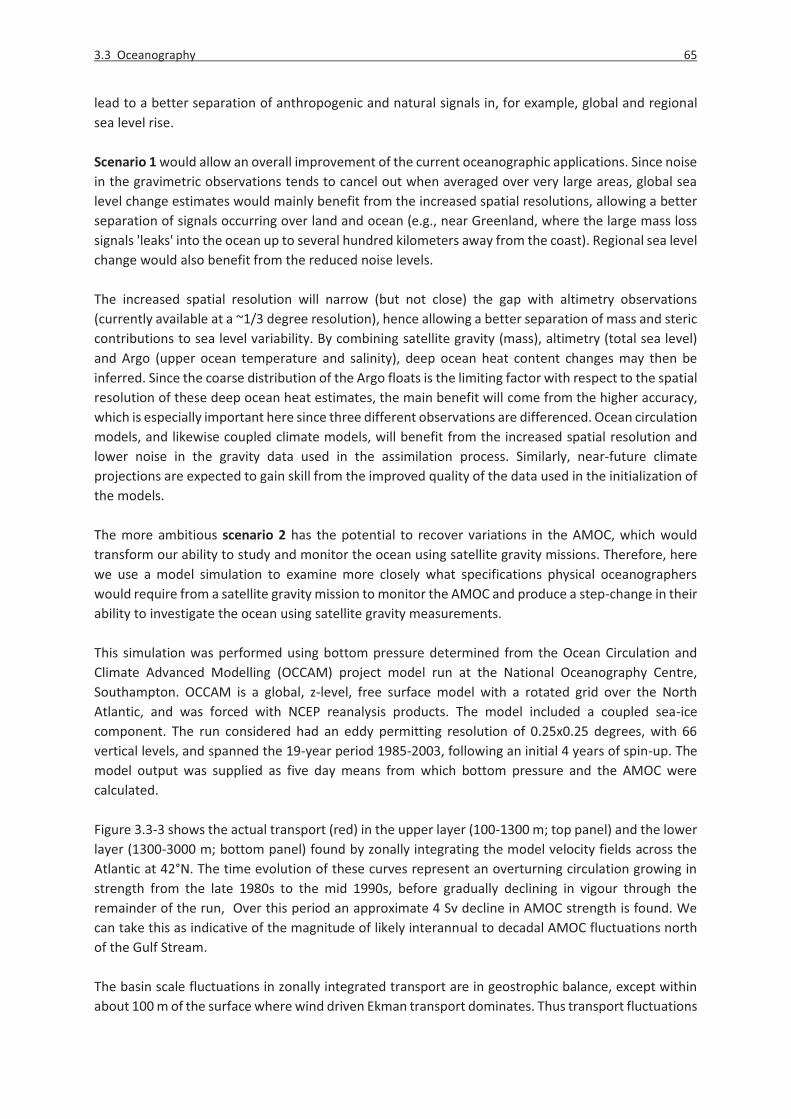
3.3 Oceanography 65
lead to a better separation of anthropogenic and natural signals in, for example, global and regional sea level rise. Scenario 1 would allow an overall improvement of the current oceanographic applications. Since noise in the gravimetric observations tends to cancel out when averaged over very large areas, global sea level change estimates would mainly benefit from the increased spatial resolutions, allowing a better separation of signals occurring over land and ocean (e.g., near Greenland, where the large mass loss signals 'leaks' into the ocean up to several hundred kilometers away from the coast). Regional sea level change would also benefit from the reduced noise levels. The increased spatial resolution will narrow (but not close) the gap with altimetry observations (currently available at a ~1/3 degree resolution), hence allowing a better separation of mass and steric contributions to sea level variability. By combining satellite gravity (mass), altimetry (total sea level) and Argo (upper ocean temperature and salinity), deep ocean heat content changes may then be inferred. Since the coarse distribution of the Argo floats is the limiting factor with respect to the spatial resolution of these deep ocean heat estimates, the main benefit will come from the higher accuracy, which is especially important here since three different observations are differenced. Ocean circulation models, and likewise coupled climate models, will benefit from the increased spatial resolution and lower noise in the gravity data used in the assimilation process. Similarly, near-future climate projections are expected to gain skill from the improved quality of the data used in the initialization of the models. The more ambitious scenario 2 has the potential to recover variations in the AMOC, which would transform our ability to study and monitor the ocean using satellite gravity missions. Therefore, here we use a model simulation to examine more closely what specifications physical oceanographers would require from a satellite gravity mission to monitor the AMOC and produce a step-change in their ability to investigate the ocean using satellite gravity measurements. This simulation was performed using bottom pressure determined from the Ocean Circulation and Climate Advanced Modelling (OCCAM) project model run at the National Oceanography Centre, Southampton. OCCAM is a global, z-level, free surface model with a rotated grid over the North Atlantic, and was forced with NCEP reanalysis products. The model included a coupled sea-ice component. The run considered had an eddy permitting resolution of 0.25x0.25 degrees, with 66 vertical levels, and spanned the 19-year period 1985-2003, following an initial 4 years of spin-up. The model output was supplied as five day means from which bottom pressure and the AMOC were calculated. Figure 3.3-3 shows the actual transport (red) in the upper layer (100-1300 m; top panel) and the lower layer (1300-3000 m; bottom panel) found by zonally integrating the model velocity fields across the Atlantic at 42°N. The time evolution of these curves represent an overturning circulation growing in strength from the late 1980s to the mid 1990s, before gradually declining in vigour through the remainder of the run, Over this period an approximate 4 Sv decline in AMOC strength is found. We can take this as indicative of the magnitude of likely interannual to decadal AMOC fluctuations north of the Gulf Stream. The basin scale fluctuations in zonally integrated transport are in geostrophic balance, except within about 100 m of the surface where wind driven Ekman transport dominates. Thus transport fluctuations

66 3 Derivation of requirements for main thematic fields
are proportional to the difference in pressure between eastern pe and western pw boundaries, with the zonally integrated transport T as a function of depth z given by
T(z) = (pe(z)-pw(z))/ρ0f0 ≈ -pw(z))/ρ0f0 where ρ0 is the average seawater density and f0 is the Coriolis parameter at the latitude of interest. In fact, Bingham and Hughes (2008, 2009) have shown that in the model interannual to decadal pressure changes on the eastern boundary are negligible and can thus be neglected. As a result it is possible to determine the transport fluctuations quite accurately at sub-polar latitudes north of the Gulf Stream using only pressure from the western boundary. This is illustrated by the blue curves in Figure 3.3-3 which show the transport fluctuations in each layer estimated from the western boundary pressure according to the equation above. Assuming this relationship between transport fluctuations and western boundary pressure changes observed in the model to be an accurate reflection of reality, it provides a clear target for what a gravity mission must achieve if it is to deliver bottom pressure changes with sufficient accuracy and spatial resolution to allow the zonally integrated transport to be monitored and studied. Here we focus on the western boundary pressure signal on the lower (1300-3000 m) part of the continental slope. This is associated with deep return flow of the AMOC and may correspond to fluctuations in the deep western boundary current. Although somewhat weaker than the upper slope transport, it would in practice be less affected by leakage from continental hydrology changes. In this case a 1 Sv increase in the southward flow corresponds to approximately 1 cm (eq. water height) drop in bottom pressure on the lower part of the slope. Figure 3.3-4 a (red) shows the western boundary pressure signal averaged over the lower 1300-3000 m part of the continental slope which has a lateral extent of approximately 80 km. This represents the signal we wish to recover. To test the ability of a gravity mission to recover this AMOC bottom pressure signal, the global ocean bottom pressure fields were expressed as a set of spherical harmonic coefficients. The bottom pressure was then reconstructed on the global grid, and the maximum degree and order at which the spherical harmonic expansion was truncated ranging from d/o=0 to d/o=200, corresponding to spatial scales of 100 km or greater. Figure 3.3-4 a (blue) shows the bottom pressure time series recovered for d/o=200. The true signal is well reproduced, accounting for 95% of the total variance. The rate of reproduction (percent of variance accounted for) is reduced when truncating the series at lower d/o. The rate of reproduction is a still reasonable 80% for a truncation at d/o=150 (Figure 3.3-4 a, dark grey), but only 30% at d/o=100 (light grey). In the latter case, this estimate of the bottom pressure signal would be of little value for monitoring the AMOC. Since the observations will contain a certain amount of noise (Table 1-1), some form of filtering will be necessary, reducing the potential to fully recover the AMOC signal (Figs. 3.3-4 b and c). Figure 3.3-4 b (green) shows the influence of Gaussian filtering with a half-wave radius of 70 km as a function of d/o. This is the maximum filter radius for which a skill score of greater than 50% is obtained, in this case at d/o=170. Figure 3.3-4 c shows how the skill of reproduction rapidly decreases as the filter radius is increased for the three truncations presented in Figure 3.3-4 a. For a mission delivering coefficients to d/o=200 (blue) the maximum filter radius that can be sustained before the recovered signal becomes useless is approximately 65 km, while for d/o=150 it is just 60 km. Clearly the ability to recover a useful signal places a very tight constraint on the level of filtering that could be tolerated. This is not surprising given the spatial scale of the signal we are trying to recover.

3.3 Oceanography 67
Figure 3.3-3: (a) Inter-annual fluctuations in the total upper layer (100-1300 m) zonally integrated meridional transport at 42N in the Atlantic in OCCAM (red) and as estimated from the bottom pressure variations on the western continental slope (blue). (b) As in (a) but for the lower layer (1300-3000 m). Based on this study, we try to derive the potential of scenario 2 to recover the AMOC. We have shown that noise-free gravimetric observations up to degree/order 200 would allow recovery of changes in the AMOC strength with a skill of reproduction of about 0.95, which gradually decreases as the maximum degree/order decreases and drops below 0.50 at degree/order 120 (Fig. 3.3-4 b). Taking into account additional filtering for noise reduction, monthly observations of the AMOC variability are therefore unlikely to be achieved under this scenario, but the noise may be reduced by averaging the observations over longer time periods, which would allow retrieval of interannual AMOC variations.
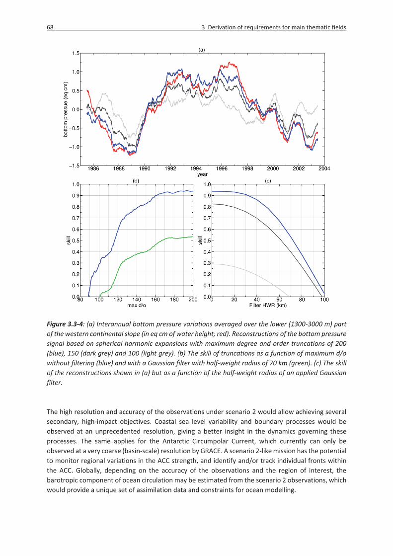
68 3 Derivation of requirements for main thematic fields
Figure 3.3-4: (a) Interannual bottom pressure variations averaged over the lower (1300-3000 m) part of the western continental slope (in eq cm of water height; red). Reconstructions of the bottom pressure signal based on spherical harmonic expansions with maximum degree and order truncations of 200 (blue), 150 (dark grey) and 100 (light grey). (b) The skill of truncations as a function of maximum d/o without filtering (blue) and with a Gaussian filter with half-weight radius of 70 km (green). (c) The skill of the reconstructions shown in (a) but as a function of the half-weight radius of an applied Gaussian filter. The high resolution and accuracy of the observations under scenario 2 would allow achieving several secondary, high-impact objectives. Coastal sea level variability and boundary processes would be observed at an unprecedented resolution, giving a better insight in the dynamics governing these processes. The same applies for the Antarctic Circumpolar Current, which currently can only be observed at a very coarse (basin-scale) resolution by GRACE. A scenario 2-like mission has the potential to monitor regional variations in the ACC strength, and identify and/or track individual fronts within the ACC. Globally, depending on the accuracy of the observations and the region of interest, the barotropic component of ocean circulation may be estimated from the scenario 2 observations, which would provide a unique set of assimilation data and constraints for ocean modelling.
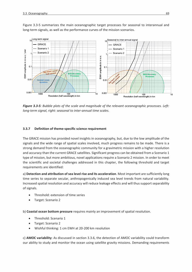
3.3 Oceanography 69
Figure 3.3-5 summarizes the main oceanographic target processes for seasonal to interannual and long-term signals, as well as the performance curves of the mission scenarios.
Figure 3.3-5: Bubble plots of the scale and magnitude of the relevant oceanographic processes. Left: long-term signal, right: seasonal to inter-annual time scales.
3.3.7 Definition of theme-specific science requirement The GRACE mission has provided novel insights in oceanography, but, due to the low amplitude of the signals and the wide range of spatial scales involved, much progress remains to be made. There is a strong demand from the oceanographic community for a gravimetric mission with a higher resolution and accuracy than the current GRACE satellites. Significant progress can be obtained from a Scenario 1 type of mission, but more ambitious, novel applications require a Scenario 2 mission. In order to meet the scientific and societal challenges addressed in this chapter, the following threshold and target requirements are identified:
a) Detection and attribution of sea level rise and its acceleration. Most important are sufficiently long time series to separate secular, anthropogenically induced sea level trends from natural variability. Increased spatial resolution and accuracy will reduce leakage effects and will thus support separability of signals.
� Threshold: extension of time series � Target: Scenario 2
b) Coastal ocean bottom pressure requires mainly an improvement of spatial resolution.
� Threshold: Scenario 1 � Target: Scenario 2 � Wishful thinking: 1 cm EWH at 20-200 km resolution
c) AMOC variability: As discussed in section 3.3.6, the detection of AMOC variability could transform our ability to study and monitor the ocean using satellite gravity missions. Demanding requirements

70 3 Derivation of requirements for main thematic fields
on spatial resolution and accuracy are necessary to achieve this goal. A little less stringent requirements enable at least detecting interannual variability of AMOC.
� Threshold: Scenario 2 � Target: Scenario 2 (to map interannual variability), better than Scenario 2 (to achieve monthly
resolution) � Wishful thinking: 1 cm EWH at 20-200 km resolution
d) Improved tidal models by co-estimation of ocean tide parameters requires long time series as well as increased accuracy compared to the current state.
� Threshold: Scenario 1 � Target: Scenario 2 � Wishful thinking: sub-daily observations, 10 cm EWH at 100 km resolution
e) Improved heat and mass redistribution observations require mainly improved spatial resolution, in association with improved accuracy, in order to separate mass and steric effects, and to understand air-ocean heat fluxes and the heat budget of the ocean.
� Threshold: Scenario 1 � Target: Scenario 2 � Wishful thinking: matching altimetry, monthly observations at 1/3 degree resolution and
~5 cm EWH accuracy f) Improved ocean circulation models. Improving the spatial resolution and lowering the noise level will lead to stronger constraints and improved ocean circulation estimates when assimilating gravity data into ocean circulation models.
� Threshold: Scenario 1 � Target: Scenario 2 � Wishful thinking: matching model resolution, O(100 km) globally to O(10km) regionally.
g) Improved near-future climate forecasts: This will lead to a better understanding and prediction of decadal fluctuations in surface temperatures and precipitation, thus providing essential information to policy makers for social and economical planning and decision making. Both improved resolution and accuracy are required to achieve this goal.
� Threshold: Scenario 1 � Target: Scenario 2 � Wishful thinking: matching model resolution, O(100 km)
h) Understanding and prediction of decadal fluctuations and secular changes in global mean surface temperature
� Threshold: Scenario 1 � Target: Scenario 2 � Wishful thinking: matching model resolution, O(100 km)

3.4 Solid Earth 71
3.4 Solid Earth 3.4.1 Societal challenges related to solid Earth In the investigation of the solid Earth with a future satellite mission, four scientific focus themes have been identified, each of which contributes to solving key societal challenges. Here these challenges and the proposed methodology to address the issues are briefly described.
A) Natural hazards associated to earthquakes, tsunamis, volcanoes
Gravity observations from a future satellite mission can provide new inputs to monitor the seismic cycle and thus improve knowledge of the risk to human life and property associated to natural hazards. This involves the estimation of the mass movement during and after magnitude 7 earthquakes, as well as the knowledge of interseismic deformation. Satellite gravity brings unique information, as traditional observations (seismographs and geodetic measurements) are often insufficient to characterize undersea and deep earthquake sources, yet crucial for knowing the seismic and tsunami risks.
B) Understanding climate changes
A new gravity mission could contribute to an enhanced quantification of the present day ice sheet loss by improving its separation from the ongoing solid Earth deformation in response to the last deglaciation, i.e., the post glacial rebound (GIA) signal. A better separation of present day water (ice or ocean) mass variations from the GIA effect will also contribute to improve our understanding of sea level variations. Ice loss and sea level variations are essential indicators of present climate changes.
C) Sustainable exploitation of natural resources
GOCE has contributed to describing the Earth’s crust in terms of density variations and geometry. This information improves our knowledge on the geology and therefore allows us to identify natural resources deposits. A new challenge is the monitoring of mass movements related to the extraction and immission of fluids when exploiting natural resources. An improved satellite mission would provide innovative means to monitor the underground fluid movements related to the exploitation process.
D) The physical properties in the deep interior, and their relationship to deep and shallow geodynamic processes
Tectonic processes leading to earthquakes, volcanoes, mountain building, mineral production, and hydrocarbons formation are linked to deep mantle and crustal processes. Thus, the understanding of the risks associated with natural hazards, as well as a sustained use of our planet’s resources in the long term, rely on the knowledge of the interior structure and dynamics of the Earth. A future satellite gravity mission would contribute to create a 4D Earth model that addresses the target of understanding and predicting near-surface motion and deformation by linking them to the underlying geodynamic processes.
In the following the scientific topics that allow to contribute to the above defined societal challenges are discussed in detail.

72 3 Derivation of requirements for main thematic fields
3.4.2 Scientific questions and challenges and their relation to gravity field signals
From surface to depth, the solid Earth is a mostly hidden, but the largest component within the Earth system. It may be divided into a surface crustal layer overlying a predominantly viscoelastic mantle, a fluid outer core and a solid inner core. The elastic and viscous behavior implies time scales of deformations ranging from < 1 second to thousands of years and up to many tens of millions of years. The solid Earth interacts with our near-surface environment in many different ways. Heat and mass (including water) are continuously exchanged between the surface and the deep, slowly cooling Earth’s interior. Volcanism releases water and gases into the atmosphere, while surface landscapes are ultimately shaped by Earth’s internal dynamics – very slowly, in the case of mountains building, on moderate time-scales for glacial isostatic adjustment, and episodically, or instantaneously, in the case of earthquakes. The deep driving forces of the mantle interact with crust and surface processes, such as active faulting, erosion, or surface mass fluxes due to (de)glaciation. These interactions reflect couplings between processes at different spatial and temporal scales, from the deeper mantle to the shallower layers of the crust, and the Earth’s gravity field reflects all these processes and their temporal evolution.
Several critical issues for society are highly relevant with solid Earth dynamics. They range from the mitigation of, or adaptation to risks from natural hazards, to the evolution or depletion of its energy, mineral and water resources. Knowing how underground fluids are distributed and move requires knowledge of the permeability of Earth’s crust, among other properties. Topics relevant for climate and environmental change are also concerned, as the climatic system inevitably interacts with the solid Earth: at the Last Glacial Maximum, ancient ice sheets in the northern hemisphere and in Antarctica depressed the Earth’s surface by several hundreds of meters. Climate and climate-driven erosion contribute to continuous shaping of mountain ranges and to other redistribution of surface loads (e.g. ice sheet melting and the corresponding sea level changes) to which the solid Earth instantaneously responds as a result of loading causing topography changes.
To address global societal concerns and urgencies about natural hazards, about sustainable supply of energy and mineral resources, and about environmental changes, with a goal to improve prediction capabilities and to apprehend the evolution of the geosphere and its habitability at the human time scale, we need to have a better understanding of the underlying dynamic processes in the crust and mantle, and how they interact with each other over a wide range of spatial and temporal scales. This requires a multi-scale, three-dimensional and time-varying imaging, as well as dynamic modeling of the Earth’s interior, to describe how the variations of Earth’s structure and physical properties affect our near-surface environment and to provide clues to the relevant statistics that characterize their time-dependence. Here we summarize scientific challenges and the associated benefits to society, which cannot be fully addressed at present.
a) A first challenge deals with monitoring Earth’s tectonic activity, aiming to understand the geophysical processes that can trigger catastrophic events: seismic activity, volcanism and landslides. The general consensus is that the lack of quantitative observations covering sufficient temporal and spatial scales of the relevant geophysical processes is limiting our capability towards understanding, modelling and possibly predicting the occurrence of such kinds of natural hazards. The tectonic plate movements are complex, as revealed by geodetic surface observations including GNSS and synthetic aperture radar (SAR) interferometry (InSAR). At subduction zones, where plates descend into the mantle, these data have shown that subduction is not a continuous process and that the subduction interface is generally a mosaic of freely slipping (i.e. creeping) patches and locked zones. The locked zones are continually loaded by slippage on creeping patches, which may be distributed over a wide

3.4 Solid Earth 73
depth range (from the ocean-bottom trench to the transition zone typically >~30 km deep) and may proceed at irregular intervals (steady creep versus episodic tremor and slip). When the accumulated stress on locked or partially locked patches becomes larger than a threshold, it is released by an earthquake or by an aseismic movement with highly variable speeds over a range of time scales, possibly as long as several years (Schwartz 2007). Because they modify the state of stress, aseismic motions might be responsible for earthquake triggering, and the interactions between these two modes of deformations remain poorly understood. Moreover, earthquakes themselves are complex phenomena: slow earthquakes release stress with a rupture propagation including low velocity components, while ‘silent’ earthquakes release stress without emitting seismic waves (Dziewonski and Gilbert 1974). Thus, seismic earthquakes express only a part of the total energy released, and a full understanding of the seismic cycle cannot be obtained only from seismic data. Complementary and critical observations for earthquake studies have currently been provided by GNSS geodetic networks and InSAR measurements, by geological and geophysical studies.
However, their spatial coverage is often insufficient for monitoring the complete breadth of deformations that encompass the entire interplate boundary. In addition, it is often difficult to obtain any observations of seafloor deformation, which would provide key constraints on the size and extent of tectonic stress accumulation, the undersea earthquake source process and possible resulting tsunami generation.
Because of its homogeneous spatial coverage and its unique sensitivity to the solid Earth interior mass displacement, both seismic and aseismic, as well as over land and at seafloor, satellite gravity can provide important information for monitoring the entire seismic cycle and understanding how stress accumulates and is released. Gravity data are especially efficient for undersea earthquakes and mass redistribution at the Earth’s surface and within its interior. This results in potentially improved early warning response time of seismic events and advances in protection of property and human life. Moreover, to describe the state of locking of the faults, and to better assess seismic and tsunami hazards, it is necessary to understand the post-seismic processes and the role of visco-elastic relaxation, post-seismic creep and other processes. Indeed, surface deformations associated with earthquake activity can arise from localized slip at depth, and/or from viscous flows over broad volumes triggered by coseismic stress changes. The relative importance of these processes is currently in debate, as it has been for more than three decades. Potential observations of post-seismic mass displacements by satellite gravity could provide key information to assess the role of aseismic-slip and broadscale-flow processes following great subduction zone earthquakes and provide one-of-a-kind first order observations at shallow, intermediate and deep levels along the subducting slab.
The non-elastic constitutive nature of the solid Earth is difficult to quantify as it involves a broad set of time scales, ranging from the periods of damped seismic waves to the scales of thermo-chemical mantle convection. In its simplest approximation at longer time scale, we can think of the Earth behaving as a Newtonian fluid with a large viscosity. With this simple approximation we struggle with constraining the viscosity and its spatial variability. Yet, the mantle viscosity is key to modeling the deformation of the mantle and crust, as it controls the velocity of convective flow and associated heat transport, the viscous deformations of the Earth in response to various internal and external forces, and the stress distribution in the lithosphere at plate boundaries as well as plate interiors. Laboratory experiments of rock deformation are one avenue for inferring the Earth’s viscosity, as realistic mantle temperatures and pressures are approachable. Besides, rheology depends on strain rate and water content. The role of these factors is not well constrained especially at high temperature and for very slow long-time strain. These limitations make geophysical observations of gravity changes after earthquake stress drop or due to glacial load change extremely important to infer the rheological properties of both the crust and mantle.
74 3 Derivation of requirements for main thematic fields
b) The Glacial Isostatic Adjustment (GIA) process is gravity driven and also alters the Earth’s gravity field as a consequence of viscoelastic mass redistribution after a long temporal history of (de)glaciation, and as the Earth’s mantle redistributes mass, the sea-level or the geoid also changes as a result of the GIA process. The ice (un)loading component may originate from the Late Pleistocene global glacial period, the Little Ice Age, or deglaciation during the Anthropocene. Despite observations such as geological and glaciological indicators of paleo sea-level, GNSS/GPS and tide-gauge measurements, determinations of GIA and inferences of Earth’s rheology remain ambiguous. Moreover, measuring GIA is difficult because many regions where we would expect to observe the viscoelastic response to the melting of the Pleistocene- and Neogene-age ice sheets and ice fields are located at or near present-day large ice sheets or glaciers. These regions are also affected by elastic surface displacements due to present day ice mass variations, e.g. in Alaska, West Antarctica, Greenland and Patagonia (Ivins and James 1999, Larsen et al. 2005, Kahn et al. 2008, Ivins et al. 2013, Nield et al. 2014, Lange et al. 2014, Mémin et al. 2014). For Antarctica, limited accessibility to rock outcrop and spatially limited paleo constraints for delivering reliable GIA models (Whitehouse et al. 2012, Ivins et al. 2013) mean that we must now use a host of interdisciplinary observations to fill this gap (e.g., Sasgen et al. 2013, Gunter et al. 2014). Current uncertainties in the GIA corrections overprint ice mass variations in Antarctica: the GIA signal could account for nearly the entire Antarctic ice-loss signal interpreted from GRACE (e.g., Velicogna and Wahr 2006, King et al. 2012). They also affect how we reconcile sea level rise observations, as the gravitational effect of GIA produces a signal of about 1 mm/yr EWH (EWH: Equivalent Water Height) on the sea level when integrated over the ocean, and presently has uncertainties of about half that size (Tamisiea 2011, Guo et al. 2012, Ivins et al. 2013).
A second challenge of a new gravity mission with improved accuracy and resolution is to contribute to the regional separation of present-day ice-mass changes from GIA, and provide valuable data to be included in GIA modelling. Areas where the GIA signal has a smaller magnitude and spatial extent might also be considered, provided overprinting signals can be well modelled – for instance where ice thickness changes in the last 500 years could result in significant present-day uplift rates or where a low-viscosity layer is present at shallow depths. Examples of regions with lower viscosity include the global seafloor, subduction wedges, continental sites of oceanic ridge subduction and mantle hot-spots. Thickness of the mechanical lithosphere and flexural rigidity is another information retrievable from gravity in combination with seismic tomography which influences the amplitude of the GIA response. It is also possible that combined space geodetic techniques, that include advanced time-varying and static gravity observations, might provide the criteria for potentially separating ongoing ice mass balance signals from GIA (Sasgen et al. 2013; Gunter et al. 2014).
c) A third challenge is to decipher geodynamic processes involved in the creation, evolution and destruction of Earth’s crust and how they are coupled to the climatic system – through processes of erosion and sediment transport for instance, that remove crust and induce isostatic uplift, or through the influence of water on rock rheology. It is indeed the very existence and stability of a continental crust that makes Earth habitable by terrestrial life, and this shallow layer holds essential resources for mankind. Over the continents, this includes all processes of mountain range building, from those having extensional origins to those involving compression. Another important challenge is to monitor and understand the rise of mantle plumes that can lead to super-volcanoes. Over the oceans, the monitoring of uplift at spreading ridges can provide new information about the processes involved in magma ascent and sea-floor generation. The gravity signature of this uplift and associated magma mass transfers, and hence their impact on the mean sea-level, is otherwise inaccessible using satellite altimetry measurements due to a lack of accuracy and the limitation to resolve long wavelength gravity signals.
3.4 Solid Earth 75
d) The fourth challenge is dedicated to the exploration and evolution of Earth’s natural resources, including geothermal energy, minerals, hydrocarbons and water. First, we need to locate the resources. For the latter, their finding is closely related to the geologic history, the type and age of the crust, its evolution in time and present geometry; the geologic evolution is closely linked to the geodynamic evolution of the building blocks of the continent, the oldest components of which are the cratons, leading to the assembly and break-up of the proto-continents. Cratons are nearly indeformable parts of the lithosphere around which deformation occurs through rifting, sedimentation and mountain range building since the Proterozoic. Their margins thus have been the location of crustal shortening, subduction and rifting, producing the metamorphic and magmatic rocks that are essential for mineral production and the sedimentary basins formations that can develop to hydrocarbon reservoirs. These processes induce density changes in the rocks, as sediments have low density while rifting and orogenesis may lead to rock densification through magmatism and metamorphism. The related density changes lead to spatial gravity field variations. Therefore gravity contributes to high resolution crustal imaging in terms of rock density. A cross-plate mapping of all the geologic features linked to density variations would be extremely useful to identify signals matching known natural resources and to define the geometry and depth of the density units, bringing clues on the geodynamic evolution. Currently there still exists a gap between very high resolution terrestrial and marine gravity maps and those recovered from dedicated satellite gravity missions at larger scales, such as GOCE. Higher spatial resolution of satellite gravity will help to bridge this gap especially in poorly surveyed areas or regions with low-quality land gravity data. The findings will guide the location selection for the detailed land investigations which are very time consuming and costly. A general idea of the regional scale structures will allow us to improve the success rate of these detailed land investigations. Moreover, for hydrocarbon exploration, a mapping of the transition between continental and ocean crust is crucial, yet it cannot be reliably recovered from satellite altimetry when close to the coast. Thus, a homogeneous gravity field with no loss of continuity from continents to ocean is needed.
A sustained exploitation of natural resources requires monitoring the evolution of underground fluids and their interaction with the solid Earth. For instance, excessive water pumping from deep aquifers can lead to the collapse and cementation of the voids that provide the Earth’s crust with a finite permeability and porous nature. Such collapse prevents the aquifer from further replenishment and constitutes an enormous danger for the long-term availability of freshwater. Pumping or extraction leading to changes in the volume of underground fluids furthermore has been connected to induced seismicity and subsidence effects. Combined with the modeling of the crustal deformation, in particular the poroelastic effects, and of the stress field induced by the underground fluids extraction, observation of mass changes in areas where such fluids are present (be they water or oil) could contribute both to assessing their distribution, the hazard of induced seismicity and deformation associated to their exploitation, and to modeling their evolution.
e) The fifth challenge is to relate near-surface motions and changes to deeper Earth mantle properties and dynamics. Naturally, these are coupled to large thermal and chemical exchange with the core. Understanding the physics of shallow and near-surface transport of solid Earth materials thus requires a global geodynamic modelling of the Earth. These models may include the manifestation of superplumes emanating from the core-mantle boundary (e.g., Campbell and Griffiths 1990, Larson 1991, van Keken 1997, Wignall 2001). The observational information that a gravity mission might provide is useful in two substantial and unique ways. The first is by highlighting the mass transport globally, over continents and oceans, as proxies for the above discussed processes. The second is that an improved time-variable gravity field also improves the determination of the long-term component of gravity and its spatial gradients. In a multi-disciplinary perspective, this can advance knowledge on

76 3 Derivation of requirements for main thematic fields
the mantle mass structure and its links to lateral variations of temperature and composition, helping to decipher the nature and the scales of the mantle convection and their interplay with the near-surface evolution. For instance, this would allow researchers to link the seismicity at plate boundaries to the structure of the mantle and to understand the evolution of the asperities at the moving plates interface, a key point in seismic hazard assessment. For this purpose, the unique geometric sensitivity of gravity gradients makes them very complementary to seismic tomography. A regionalized imaging of the mantle physical properties would also allow us to more accurately model its elastic and viscous deformations in response to various excitations, a pre-requisite to take the best of high accuracy measurements of mass displacements within the Earth’s system.
The coupling of the mantle to the core and the core dynamics are the most challenging topics. Observing gravity perturbations associated to the oscillation modes of the core would shed light on parameters of the Earth’s deepest interior such as the density contrast and the flattening at the inner core boundary, the magnetic friction at the fluid core boundary as well as the effective viscosity of the inner core. They include the Slichter modes, resulting from oscillations in translation of the solid inner core around its equilibrium position (after a very large earthquake for instance), or the rotational eigenmodes of the inner core. Observing the oscillation modes in the fluid core, the excitation mechanisms of which are not well identified, would allow to constrain the viscosity of the outer core, to test the excitation models, and to bring information on the dynamic (in)stability of the fluid core. However, it is highly unlikely if not impossible that spaceborne gravimeters detect the Slichter modes. At sub-decadal time scales, the origin of geomagnetic jerks is still poorly understood; information on core flows through time variations of gravity would help constrain the physical mechanism behind these sudden changes in Earth’s magnetic field.
3.4.3 Relevant temporal and spatial scales
The spatial and temporal scales associated to the abovementioned processes are summarized in Table 3.4-1, and discussed hereafter.
� Concerning the seismic cycle, a study of geoid variations at GRACE resolution associated with earthquakes of varying magnitude can be found in de Viron et al. (2008). A higher spatial resolution and accuracy is needed to detect the gravitational changes associated with earthquakes of Mw 7 to 8.
� Concerning GIA signals, the largest geoid change is found in the Hudson Bay area with around 1.3 mm/yr (Rangelova & Sideris, 2008). However, elsewhere GIA signals in smaller areas and with smaller amplitude exist which require a significantly higher accuracy and higher spatial resolution (Ivins et al., 2011; Zhang & Jin, 2013; Root et al., 2014).
� Concerning the oscillation modes of the core: the Slichter modes have a 2-6 hours period, and the amplitude of the gravity perturbation induced by an earthquake at these periods has been estimated to about the nanogal (Crossley 1992, Rosat 2007). The amplitude of the gravity perturbations induced by the rotational eigenmodes of the inner core (Mathews et al. 2002) is weak (about 1 nGal) due to the small size of the inner core, and there is atmospheric noise around this period. At sub-decadal time-scales, core fluid flows can contribute to time variations of the gravity field by advection of a density heterogeneity (Dumberry 2010), or due to the dynamic pressure at the core-mantle boundary caused by the flows, which deforms the overlying mantle (Greff-Lefftz et al. 2004). Large-scale gravity anomalies of magnitude ~100 nGals can be obtained.

3.4 Solid Earth 77
Table 3.4-1: Spatial and temporal scales associated to gravity changes relevant to solid Earth investigations. FCN: Free Core Nutation, FICN: Free Inner Core Nutation. CMB: Core-Mantle Boundary.
Signals Time scales Expected signals: temporal variation in geoid, or gravity
Spatial scale
Earthquakes (Mw 7-9) Coseismic
instantaneous 0.1 to 1 mm geoid or 5 μGal
Geoid amplitude decrease by > 10 times when Mw reduced by 1
Mw 9: > 300 km Mw 8: 200-300 km Mw 7: 60-130 km
Earthquakes (Mw 7-9) Post-seismic
up to decades 0.01 to 0.1 mm geoid change/yr or 1 μGal/yr
same as above
Slow & silent earthquakes
up to years Possibly periodic
can be equivalent to a Mw 6-7 earthquake (Hirose et al., 1999)
~100 – 200 km
Glacial Isostatic Adjustment
decades up to secular
1 mm/yr geoid
from global to tens of km
Mantle convection & global scale plate tectonics
secular sinking slabs: < 0.005 mm/yr
1,000 km
Mid-ocean ridges secular
0.5 mGal/yr few 10 km
Regional plate tectonics, mountain building, crustal thickening at a rate 0.1 – 2 cm/yr
decades to secular
2 μGal/yr
10 km to few 100 km
Subsidence or emergence of volcanic islands; fast movements in volcanic regions
decades to secular, also higher rates possible
0.1 to 1 μGal/yr
local: few km to few 10 km
Core motions, magnetic pressure at the CMB
years 100 nGal (large uncertainty exists)
large-scale
Slichter mode, FCN, FICN
hours 1 nGal
large-scale
Seismic normal modes < 1 hour 1 nGal
large-scale
� The order of magnitude for gravity signals due to crustal thickening can be derived considering the example of the Tibetan plateau, where horizontal convergence is 3-4 times the uplift rate. The absolute gravity rate at Lhasa set at the South-Eastern part of the plateau is 1.97 � 0.66 μGal/yr, and when corrected for the uplift and assumed erosional denudation remains negative at a rate of -1.56 � 0.67 μGal/yr. The residual negative gravity rate has been interpreted as the observation of crustal thickening, in terms of Moho deepening, at a rate of 2.3 � 1.33 cm/yr (Sun et al. 2011).
3.4.4 Achievements and limitations of current gravity missions
The achievements of satellite gravimetry have been spectacular for the two missions GRACE and GOCE, which are complementary. The time varying gravity field from GRACE has contributed significantly to the modeling of the GIA signal and to the observation of mass redistribution at the site of great subduction zone earthquakes. Correlations between time variations of the gravity and magnetic fields have also been observed. GOCE was designed for modeling the static gravity field at improved

78 3 Derivation of requirements for main thematic fields
resolution. This static field has given new results in the knowledge of crust, lithosphere and mantle, useful for geodynamics, exploration and seismic hazard evaluation. A further application of the improved gravity field is the unification of national height systems, one of the goals of GOCE. In the following some results are summarized, going from the faster to the slower processes.
� At time scales of years and less, achievements from GRACE can be cited for the monitoring and
understanding of the seismic cycle. Co-seismic and post-seismic gravity variations associated to large earthquakes (Sumatra 2004, 2005, Bengkulu 2007, Maule 2010, Tohoku-Oki 2011, Indian Ocean 2012) have been detected and allowed to test candidate co-seismic rupture models and evidence the importance of co-seismic crustal dilatation of the upper plate (2004 Mw 9.1 Sumatra: Han et al. 2006, Panet et al. 2007, de Linage et al. 2009, Broerse et al. 2011, Cambiotti et al. 2011, Wang et al. 2012c, 2010 Maule: Han et al. 2010, Heki and Matsuo 2010, Wang et al. 2012a, 2011 Mw 9.0 Tohoku-Oki: Han et al. 2011, Matsuo and Heki 2011, Wang et al. 2012b, Cambiotti and Sabadini 2012, Zhou et al. 2012, Dai et al. 2014). Figures 3.4-1 and 3.4-2 show the co-seismic and post-seismic gravity signal induced by the Sumatra-Andaman earthquake. Not only thrust earthquakes, which are accompanied by important vertical deformations, could be detected, but also the 2012 Indian Ocean strike-slip event, involving mostly horizontal crustal displacements, was sensed by GRACE. The GRACE data analysis revealed substantial gravity change associated with compression and dilatation in four different quadrants (Han et al. 2013). The added value of satellite gravity is as follows. First, it brings information on the rupture geometry when it is ambiguously constrained from the surface networks. Such uncertainty in the rupture model is often the case for undersea earthquakes due to the limited spatial coverage of ground geodetic data, e.g., the comparison of five rupture models proposed for the 2004 Boxing Day earthquake in Sumatra based on different types of data (excluding satellite gravity) in Poisson et al. (2011). Wang et al. (2012) showed the sensitivity of GRACE to the size of the fault and the average slip in the case of the Maule earthquake. Dai et al. (2014) demonstrated the unique sensitivity of gravity signals using GRACE for the 2011 undersea Tohoku-Oki earthquake, and used GRACE data for inversion of the slip rake angle, centroid location and seismic moment to further constrain the
Figure 3.4-1: Co-seismic gravity variations (microGals) due to the Sumatra-Andaman earthquake (Han et al., 2006)
Figure 3.4-2: Post-seismic geoid variations (mm) after the Sumatra-Andaman earthquake, until 2009 (Einarsson et al., 2010)

3.4 Solid Earth 79
focal mechanism. Note that in the case of offshore earthquakes, the geographical localization of the gravity anomaly with respect to the trench can help distinguishing between deeper or shallower models of slip along the plate interface. The source depths and rigidity and bulk modulus were also understood independently from seismic and geodetic data (Cambiotti et al. 2011, Han et al. 2013). A second added value is to compute the seismic moment of the sources also including its slower components. GRACE resolved the sources on temporal and spatial scales exceeding the seismic and geodetic spectrum and confirmed the slow components for the 2004 Sumatra-Andaman earthquakes, but not for the 2011 Tohoku-Oki earthquake (Han et al. 2013). Finally, when combined with GPS data, which exhibit a different sensitivity to mass displacements as a function of depth, satellite gravity helps to assess the respective role of afterslip and visco-elastic relaxation after the earthquakes as shown by Han et al. (2008) and Panet et al. (2010) for the Sumatra earthquake and to reveal prevailing viscoelastic relaxation by Han et al. (2014a) after the 2011 Tohoku-Oki earthquake and by Han et al. (2014b) after the 2012 Indian Ocean earthquake. Deciphering the roles of these processes is important in order to infer the distribution of stress at the subduction boundary and to understand the interseismic stress loading cycle, and thus to assess seismic hazard. Constraints on the viscosity of the upper mantle could be obtained in Höchner et al. (2011), showing large rates of deformation that suggest the transient viscosity as low as 5�1017 Pa s and the steady state viscosity of 1019 Pa s – and even possibly non-linear rheologies in the upper mantle (Panet et al. 2010).
The interest and possibility of using time-varying gravity gradients for studying earthquakes was put forward through the detection of the Tohoku-Oki seismic signal in GOCE data (Fuchs et al. 2013); the acoustic waves propagated by the earthquake have been sensed by the mission accelerometers (Garcia et al. 2013). However, up to now only earthquakes with magnitude Mw greater than 8.4 could be detected from the present satellite gravity, so only a very limited amount of events could be studied. The use of gravitational gradient change observations inferred from GRACE is demonstrated to be useful for detecting higher frequency band seismic deformation by Wang et al. (2012b) on the Sumatra-Andaman earthquake, and the Tohoku-Oki earthquake (Dai et al. 2014).
� At inter-annual scales, a common mode of variability between the time variations of the gravity field from GRACE and the magnetic field secular acceleration has been evidenced in an area over Africa (Mandea et al. 2012). It suggests the interest of joint gravity/magnetic field investigation for core dynamics studies, to gain better understanding of the origin of the internal geomagnetic field.
� At decadal to secular time scales, GRACE has delivered a new kind of dataset for the measurement and modelling of the Glacial Isostatic Adjustment. Due to its spatial coverage, satellite gravimetry indeed proved to bring unique new constraints on the spatial pattern of GIA and, subsequently, on the mantle viscosity and lithospheric thickness (Paulson et al. 2007a, Steffen et al. 2012), and on the ancient ice (Tamisiea et al. 2007). In North America and Fennoscandia, where the GIA induced gravity rate is large and smooth, GRACE derived estimates of GIA are accurate (van der Wal et al. 2011; cf. Fig. 3.4-3) and uncertainties in the modeling are reduced (Paulson et al. 2007b). However, it was demonstrated by analysis of higher resolution data from the GOCE satellite that there is time-variable gravity signal at wavelengths below the GRACE resolution (Bouman et al. 2013a).
At present, we cannot separate with sufficient accuracy mass movement caused by GIA from contemporary ice sheet mass changes through GIA modelling alone (Barletta et al. 2008) and we need to consider multiple data sets (Ivins et al. 2011, 2013; Sasgen et al. 2013). Current inversions

80 3 Derivation of requirements for main thematic fields
for GIA and present-day mass changes combine GRACE data with high-resolution altimetry data (Wu et al. 2010; Gunter et al. 2014). Such combination introduces other errors and the spatial resolution is currently limited by the relatively low spatial resolution of GRACE. Gravity trend data might be able to separate present-day ice losses, which have a more localized signature, from the longer wavelength signature of viscoelastic rebound.
Figure 3.4-3: Uplift rates in Fennoscandia derived from GRACE (left) and interpolated from GPS data (right), associated to post-glacial rebound (van der Wal 2011).
� At scales of decades, relative plate movements at mountain ranges are well constrained from GPS observations. As crustal material is not destroyed, it implies that it contributes to crustal thickening, which, according to the isostatic degree of compensation, is divided into topographic uplift and crustal root growth. Sun et al. (2009) thus interpret negative gravity rates over Tibet as the observation of crustal thickening. Alternatively, Matsuo and Heki (2010) attribute the yearly and long-term gravity change to hydrologic effects concentrated at the outer border of the Tibet plateau. These authors mention the uncertainty in the contribution of isostatic or tectonic uplift, but do not consider the effect of crustal thickening. The satellite observation of mass transfer in these areas at a GOCE-type spatial resolution would deliver a useful constraint on modeling the mountain building process and reduce the uncertainties in the interpretation of the gravity signal, including the separation of the tectonic and the hydrological effects.
� Referring to the static field, gravity gradients from GOCE advanced knowledge on the interior structure and processes leading to earthquakes. The data allowed to identify asperities at the interface between moving plates, thus showing the relation between lithospheric structure and faulting. Magmatic bodies at the subducting interface alter the stress regime, leading to formation of relatively strong asperities which control the timing and spatial extent of fault rupture. The position and extent of the strong asperities determines the topography of the approaching and overriding plate. The subducted bathymetric features and the batholiths are detectable in the gravity field due to the density differences in relation to the subducting and the overriding plates (Song and Simons 2003; Tassara 2010). Using GOCE data Alvarez et al. (2014) have confirmed that the subducted bathymetric elevations control the megaquakes along the Chilean margin. Information on asperities on the fault that control rupture is necessary in the modeling of stress-

3.4 Solid Earth 81
strain and estimation of future ruptures. Immediately after an earthquake one important question is whether the main stress on the fault has been released, and what the expected maximum magnitude for the aftershocks may be. The presence of asperities on the ruptured fault is an important input in the hazard calculations. The resolution of GOCE has been estimated to resolve a batholith with 240 kg m−3 density contrast of 45 km diameter (Köther et al. 2012). Much higher resolution power is needed in the future to be able to use satellite gravimetry in subduction zone (asperity) mapping.
� Numerous improvements on the knowledge of the density variations in the crust and mantle-lithosphere have been obtained from GRACE and GOCE. The topics have been the depth variations at the crust-mantle interface (e.g., Bagherbandi and Eshagh 2012, Braitenberg and Ebbing 2009, Reguzzoni and Sampietro 2012, van der Meijde et al. 2013), evaluation of existence of magmatic crustal underplating (Kaban et al. 2010; Mariani et al. 2013), modeling lithosphere interactions at subduction zones (Köther et al. 2012), 3D lithospheric structure below the Himalayas and Tibet from a joint gravimetry-seismology inversion (Basuyau et al. 2013) and evaluation of the isostatic equilibrium (Shin et al. 2007, 2009).
All above topics are crucial in constraining the composition and evolution of the Earth’s crust-mantle system. The combined terrestrial and satellite fields as the EIGEN-models (Förste et al. 2008 and successive editions) and EGM2008 (Pavlis et al. 2012) have triggered geophysical studies covering the entire globe, although they suffer from inhomogeneities in the terrestrial data coverage (Bomfim et al. 2013).
Correlation analysis between synthetic gravity data from existing models such as CRUST2.0 and GOCE observations have demonstrated that these models must be improved. The GOCE gravity field and the gravity field of topography and isostatic models correlate at a level of 0.8 for degrees between 125 and 210, decrease remarkably for degrees both up to n=250 and less than 25, and have a systematically lower value (between 0.6 and 0.7) for degrees between 25 and 150 (Hirt et al. 2012). The correlation coefficient with the CRUST2.0 model is less than 0.4 at all degrees, demonstrating that it is presently inadequate and needs critical improvement. The 80-km resolution of GOCE is adequate at Moho level, but higher resolution is strongly required to model crustal density architecture, including superficial layers such as sedimentary basins. Satellite gravity use in this direction has so far only been attempted in combination with land geophysical data (e.g., Basuyau et al. 2013).
� Gravity is also an important observable when it comes to constrain structure and dynamics of the sublithospheric mantle. The GOCE-satellite gradients are well suited to study the upper mantle density structure, making them complementary to gravity and seismic tomography (Bouman et al. 2013b, Fullea et al. 2014, Martinec and Fullea 2014). When combined with orbit data, the Earth’s gravity gradients from GOCE are also sensitive to the large-scale structure of the upper part of the lower mantle and were interpreted to reveal sinking tectonic plates and convective instabilities between 1000 and 2500 km depth (Panet et al. 2014). In contrast to geoid data, the gradients bring an enhanced geometric characterization of the mass distribution. This opens new possibilities to study the deep mantle mass structure and dynamics in combination with seismic tomography. Chaves and Ussami (2013) inverted geoid undulations in 3D using tesseroids below the Yellowstone Province, with the aim of mapping the mantle plume. They find that the inversion is stable and that the results are complementary to the seismic tomography models in retrieving temperature and compositional changes. GRACE static gravity fields, which are of a great quality for the larger spatial scales, were also analyzed to study the lower mantle structure and to characterize thermochemical oscillating domes (Cadio et al. 2011), or to analyze the formation of bathymetric swells due to the interaction of a rising plume with the lithosphere (Cadio et al. 2012).

82 3 Derivation of requirements for main thematic fields
� With GOCE data, for the first time a satellite derived field has sufficient resolution and precision to resolve geologic units useful in geophysical exploration. Although presently only large-scale features can be identified, results in Africa (Braitenberg 2014, Braitenberg et al. 2011, Martinec and Fullea 2014), Arabian peninsula (Ebbing et al. 2013), Mediterranean (Fullea et al. 2014) and the Alps (Braitenberg et al. 2013) are encouraging. Presently only greater geologic units can be identified. Although exploration applications usually require more details, the units that have sufficient extension have been identified without any doubt and an excellent match with the geological maps has been demonstrated. Units that are disguised by recent sedimentary cover have been shown to be identified with the GOCE gravity models. The identification is crucial for planning more detailed investigations with higher resolution than GOCE. For the Congo basin Martinec and Fullea (2014) interpreted the gravity anomaly and vertical gravity gradient of the GOCE/GRACE combined gravity model to renew the existing model of sedimentary rock cover and density stratification. The Congo basin is nearly circular with a radius of 600 km, so one of the largest basins worldwide. An increase in spatial resolution would increase the number of basins that could be studied from satellite gravity.
In the underexplored Rub'al-Khali area of the Arabian Peninsula the GOCE vertical gradient was used to invert for crustal thickness (Bouman et al. 2013b). The Moho model was used to update the heat flow model and maps describing the possible existence of oil or gas in view of the thermal state of the source rock (source rock maturity maps), which were generally consistent with known source rock maturity trends in the surrounding regions. GOCE gradients were therefore shown to be useful to map crustal thickness and deep regional structures. In combination with other data, heat flow can be modeled which is essential for basin maturity evaluation.
3.4.5 Identification of potential new satellite gravimetry application fields
Beyond GRACE and GOCE, there is a wide range of scientific targets and applications for society that would greatly benefit from gravity measurements continued in the future.
a) Monitoring magnitude 7 earthquakes and induced post-seismic deformations
Earthquakes of such magnitudes are often extremely destructive and occur relatively frequently. Because of its homogeneous coverage all over the globe, satellite gravity shows a unique capability to describe these events, especially undersea earthquakes which cannot be obtained from terrestrial geodetic observations. Because of its sensitivity to both seismic and aseismic mass displacements, satellite gravity can contribute to describe the entire earthquake process, including the components beyond the seismic frequency band and aseismic creep. In addition, gravity data is inherently sensitive to the interior structure and deformation in complement to surface measurements from GPS and InSAR (Interferometric Synthetic Aperture Radar). The gravity signal produced at subduction zones by a strike-slip or dip-slip fault (dip = 15°) is shown in Fig. 3.4-4. An improved mission performance as Scenario 2 would allow to detect M 7.0-7.5 earthquakes at a resolution of 150 km. With such spatial resolution, it may be possible to distinguish afterslip on the fault from post-seismic relaxation, which has been quite difficult to discriminate based on ground GPS data. With their study on the 2011 Tohoku-Oki earthquake, Han et al. (2014a) demonstrate the importance of spatial resolution in discerning the type of post-seismic movement. Earthquakes with M > 7.5 occur every ca. 3-4 months, and for M >7.0 every month on average.

3.4 Solid Earth 83
Fig. 3.4-4: Coseismic gravity change decomposed at different wavelengths for earthquakes at subduction zones compared to the performance of the different satellite gravity mission scenarios.
For such objectives, application of spaceborne gravity requires higher spatial resolution. This would also increase the statistical likelihood of capturing a greater number of events over a space mission lifetime. For instance, a satellite mission with GOCE-type spatial resolution providing time variable gravity models could result in catching the earthquakes with magnitude Mw>7.5, which would result in up to 3 observable events per year. The use of time-varying gravity gradients would strongly enhance the geometric description of the earthquake-related mass transfer at depth, as shown by recent studies (Dai et al., 2014), helping to identify the earthquake signal from the superimposed noise and fluid components. This would be a unique capability of satellite gravity as compared to all other observations systems.
Furthermore, beyond the earthquakes and subsequent deformations, the ability of satellite gravity to monitor aseismic mass displacements over land and ocean is a unique asset in order to monitor the entire seismic cycle, including the slow movements related to stress accumulation and stress release that cannot be studied by seismology and are hardly detectable by ground geodetic networks. Extreme resolution and precision would be needed to monitor the locked asperities of subduction zones.
At subduction zones involving island arcs the geodetic monitoring is hampered by the lack of dense stations that allow monitoring the interseismic deformation process. Due to the density contrasts between crust and mantle and crust and water the deformation generates a detectable gravity signal. Although island arcs are narrow, their along strike extent is several hundreds of km, which makes detection with satellite gravimetry feasible.
The recent example on the 2011 Tohoku-Oki earthquake demonstrates the importance of enhanced spatial resolution of the satellite gravity data to discriminate between two competing postseismic processes: afterslip versus postseismic relaxation. In addition to seafloor displacement measurements,

84 3 Derivation of requirements for main thematic fields
gravity data would be able to efficiently identify differences between the two processes if the data provide a higher resolution, such as 100 km or longer, as opposed to the present GRACE spatial resolution of 333-500 km (e.g., Han et al., 2014a).
Another aspect regards the detection of the gravity field oscillation produced by seismic and tsunami waves and free oscillations. Presently seismology relies strictly on ground displacement/oscillation measurements detected by seismogram. However, earthquakes produce gravity field oscillation as much as ground shakings. The innovative analysis of satellite gravity data (instantaneous gravity perturbation measured, e.g., in range-rate change) will allow the analysis of earthquakes, seismic and tsunami waves, and free oscillation from the orbiting satellites. In order to analyze the potential, range-rate changes have been simulated along the GRACE orbits (500 km altitude) induced by the 2004 Sumatra-Andaman earthquakes in 26 December 2004. The normal modes down to 200 sec (from 0S2 with 54 min periods) were integrated to simulate the gravity perturbation along the orbit based on the centroid moment solution by Stein and Okal (2005). The computation results during the first and last 6 hours of the day are shown in Fig. 3.4-5 to highlight greater attenuation of higher frequency modes over time. The 0S2 mode shows the least attenuation and will last even for a week, perturbing continuously the satellite orbits to the level detectable by inter-satellite microwave and laser ranging. A future satellite gravity mission should allow groundbreaking seismological research based on gravitational seismogram from the orbits.
Figure 3.4-5: Transient gravity change induced by seismic waves and free oscillations of 2004 Sumatra-Andaman earthquake, manifested in inter-satellite range-rate. Simulation is based on a single centroid (M0 = 1200�10-27 dyne cm from Stein and Okal (2005)), depicted in blue. The normal modes of 200 sec or longer were used. The red line represents only the 0S2 mode (~54 min period). The earthquake occurred at around 1 hour of the day (UTC). Societal Benefits: A future gravity satellite mission with capability to detect tectonic deformation (resulting in mass movement) before, during and after earthquakes with magnitudes > 7 would bring a completely new and complementary component to assessing seismic hazard in many plate boundary regions. For example, the plate boundary region between Africa and Eurasia from the Azores to
3.4 Solid Earth 85
Anatolia, which encompasses the entire Alpine-Mediterranean region, is characterized by such major-earthquake activity often close to densely populated regions (e.g. west-Anatolian fault; central and South Italy; Gulf of Cadiz & Betic-Rif-Alboran region). The largest known mega-thrust earthquake that struck Europe was the “Lisbon earthquake” of 1755, which actually occurred in the Atlantic oceanic lithosphere south of Portugal, with an estimated magnitude of 8.5-8.7, causing a huge tsunami and widespread large destruction. The next generation gravity satellite observations would provide the missing pillar needed for advancing integrative studies of the active deformation of the wider Mediterranean plate boundary region, complementing efforts of seismology (crust-mantle structure and earthquake mechanisms), geodesy (active surface deformation), and 4-D modeling of lithosphere-mantle dynamics (linking mantle structure, active tectonic processes to crustal deformation). This example can be generalized and extended to other plate boundaries and subduction zones worldwide; the ultimate target is that future integrative and detailed 4-D deformation models must fit the detailed gravity field observations as an independent constraint on both density and structure. A necessary and key input for the seismic and tsunami hazard assessment – the latter concerning much broader areas than the subduction zone location itself - is the knowledge of the amount of ongoing interseismic deformation. In the case of subduction at remote island arcs and for deep seated faults (over 100 km depth), traditional methods including geodetic monitoring and microseismic observations fail due to remoteness and depth of source. After the earthquakes, the viscosity is the most important factor to govern evolution of the long-wavelength (large scale) stress field. It may be better characterized by observations with complete spatial coverage such as the space-based monitoring of postseismic gravity changes, leading to a better understanding of increased seismic hazard following great earthquakes.
b) Modelling of the Glacial Isostatic Adjustment
The estimates of both GIA and current ice melt, combining GRACE data with high resolution altimetry, will improve when the GRACE error is reduced and the spatial resolution increased, as well as reliable GRACE error estimation becomes available. In areas where the GIA signal has a smaller magnitude and spatial extent, much can be gained from time-variable gravity measurements with higher accuracy and increased spatial resolution. This includes areas where the GIA signal is close to the current measurement error of GRACE such as Patagonia (Ivins et al. 2011) and the Barents Sea (Root et al. 2014). Higher resolution is also necessary in areas where ice thickness changes in the last 500 years result in significant present-day uplift rate, such as Alaska (Larsen et al. 2005), Iceland (Auriac et al. 2013), Patagonia (Lange et al. 2014) and Antarctica (Whitehouse et al. 2012). Because of the timing and spatial extent of the ice thickness changes in combination with low viscosities at shallow depth, the gravity rate pattern will have more short-wavelength variations than in areas with high viscosity. Thus, higher spatial resolution in these areas is crucial either for observing GIA signals or for separating them from signal due to present-day mass changes. Such low-viscosity regions include the global sea-floor. Indeed, seafloor lithosphere has the thinnest crust on Earth, and some areas feature thinner elastic lithosphere and lower viscosity upper mantle or asthenosphere, e.g., the coastal low-viscosity zones have a depth of 20 km, a thickness of 12 km and a viscosity of 1018 Pa s. A seafloor region with low viscosity (upper) mantle would imply faster time of GIA uplift as compared to more ancient cratonic lithosphere regions. There are very few ocean-bottom geodetic instruments presently deployed, hence few observations to capture transient deformation; as altimetry cannot capture long-wavelength signals and lacks accuracy, an advanced GRACE type measurement would shed light on this geophysical process.

86 3 Derivation of requirements for main thematic fields
In continental areas, analysis of longer time spans of satellite gravity data should also allow us to separate more clearly inter-annual hydrological and cryospheric mass variations from the GIA signal. Better mass variation records will also lead to improvements in numerical modeling of GIA and cryospheric mass variations. This will enhance capabilities to simulate long-term cryospheric mass fluxes and separate them from changes induced by GIA.
Societal benefits: Quantitative description of present climate changes and predictions of the future changes are crucial for sustainable societal development. Ice loss is an essential indicator of present changes. Moreover, it is important to know which ice sheets contribute to sea level rise because ice sheets evolve differently in a warming environment. Some ice sheets may reach tipping points after which the ice loss becomes irreversible. Knowledge of sea level rise is essential for planning building and flood prevention measures in coastal regions. Both ice loss and sea level change measurements rely on the observation of height changes of the sea level or ice sheet, respectively. Conversion of the height changes to corresponding volume changes necessitates accurate knowledge of isostatic and dynamic uplift and subsidence which are one of the aims of the future gravity mission.
c) Modeling and monitoring of tectonic motions related to the processes of crust formation, evolution and destruction
This includes uplift and subsidence typical to areas of plate divergence, e.g. oceanic ridges, and convergence, e.g. mountain belts and subduction zones. In mountain belts the ongoing uplift has been measured by GPS, and rates of a few mm/yr are typical. The horizontal convergence rates at mountain ranges and subduction fronts are much greater, in the order of several cm/yr. From surface observations alone it is not possible to distinguish different processes acting at the lower crustal level such as crustal thickening, crustal ablation or lower crustal melting and metamorphism. The different lower crustal mechanisms imply mass or mass-distribution changes that are measurable. At present, the GRACE resolution is too coarse to separate the contributions from superficial, and deeper mass dynamics and crustal thickening is not detectable from present GRACE data. An increased resolution would allow to provide a greater insight into the mountain building process, with a benefit for the modeling of stress accumulation and volcanic and earthquake hazard assessment. Quantifying sediment transport is important in coastal lowlands as it negatively affects navigational routes. At volcanoes the uprising magma generates a deformation of the volcano, monitored by tiltmeters and space geodetic methods, but the mass variation can only be indirectly induced from these observations. The problem is that the characteristic wavelengths and amplitude of gravity signals are relatively small, and remain at the limit of resolution of the future satellite missions discussed here. A further benefit is the improved modeling of sediment production rate of orogens.
Societal benefits: The rate of ongoing tectonic motions is a crucial parameter that is necessary in modeling the seismic cycle as well as vertical movements induced by GIA and present ice and sea level changes. The societal benefit therefore is in the improvement of seismic hazard assessment and in the quantitative monitoring of climate change. Neglect of knowledge of mass variations and vertical movements induced by tectonic motions directly translates into errors in the estimate of seismic hazard and the volume of continental ice loss. Both issues are crucial for the planning of future society on a changing Earth.

3.4 Solid Earth 87
d) Monitoring of the natural resources and the interactions between underground fluids and the solid Earth
Groundwater storage monitoring is crucial for monitoring the fluid-volumes and for the induced changes, as deformation. 4D terrestrial gravity acquisitions aimed at CO2 sequestration or aimed at monitoring the fluid movements and the induced deformation and seismicity at hydrocarbon fields must be corrected for the background noise due to the groundwater cycle. Gravimetry has been proven efficient for hydrological studies, and has given excellent results when comparing point-wise repeated absolute gravity observations with well data and moisture probes. The GHYRAF (Gravity and Hydrology in Africa) experiment in Western Africa gave a seasonal signal up to 11 μGal, equivalent to a water storage changes of 260-mm thick infinite layer of water. The present resolution of GRACE is sufficient for monitoring storage changes only in very large basins which area approaches 2�105 km2. The time resolution should be at least 1 month at a signal level of 2 μGal (entire peak to peak signal 11 μGal, divided in four periods to evaluate the estimated variation). The mission should be planned for at least 6 years, to be able to distinguish a seasonal from a long-term signal.
Societal benefits: The net amount of underground fluids stored in the subsurface is disturbed by fluid extraction or emission affecting the underground stress equilibrium. Gravity is a mean to monitor the fluid movements and storage. Applications include natural resources monitoring and environmental issues connected with the type of fluid that is injected into the subsurface. The satellite gravity field is an integrative exploration tool able to investigate the full extent and depth of the fluids.
e) 4D dynamic Earth model
Finally, the overarching and grand research target of solid Earth Sciences for which particularly future gravity missions are becoming very important is relating the tectonic activity of the surface and near-surface crust to the internal structure and dynamics of our planet, by creating a 4D dynamic Earth model for understanding and predicting (near)-surface motion and deformation. Such a comprehensive research challenge aims to eventually integrate the large temporal and spatial scales comprising, e.g., tectonic motions and deformation, GIA and spatially variable sea-level change, and earthquake generation in an advanced model of planetary dynamics. This model integrates the 3-D heterogeneous structure and the complex non-linear rheological behavior of the crust-mantle system into a dynamically self-consistent model of the Earth. Key constraints on such a model are satellite observations of Earth’s gravity field on the widest spectrum of wavelengths and with as much temporal resolution as possible. Achieving this grand target requires a time-path of decades, but given current observational and methodological capabilities in a wide range of Earth Sciences (geology, geophysics, geodesy, surface and environmental sciences), this is achievable when future (including beyond the next) satellite gravity (and other Earth-oriented geodetic) missions provide the detailed observations necessary for integrating the local-to-global structures, processes, and dynamics in an concerted effort with solid Earth Sciences.
A new and important topic to mention in this context is the interplay between mantle and core dynamics, particularly for gaining much deeper understanding of (sudden?) intensity drops of the magnetic field lowering the Earth’s magnetic shield against devastating high-energy particles from space. Even though observing gravity signals related to core dynamics appears an extremely challenging task, a new gravity satellite mission may bring core-dynamics and core-mantle coupling into play. It requires the highest accuracy – not only in the gravity measurements, but also in the separation from other physical signals of a 4D-dynamic Earth to be reached for large spatial scales and/or very high temporal resolutions. Oscillation modes of the core appear to occur with very short
88 3 Derivation of requirements for main thematic fields
periods and with extremely small amplitude and thus constitute a very ambitious target. Possible signals correlating with geomagnetic field variations (magnetic jerks) should be slower, but with a possibly larger (but still small) amplitude. The cause for strong magnetic field intensity variations (eventually leading to the switch between Magnetic North and South poles) are not well understood and may correlate with any inner-outer core dynamics and/or coupling between core and mantle dynamics.
3.4.6 Added value of individual mission scenarios
As discussed in the previous sections, GRACE has demonstrated the detection of solid Earth signals associated to GIA and to earthquake-related deformation and hydrologic signals, but a higher spatial resolution is necessary in order to make a leap forward in solid Earth sciences. Mikhailov et al. (2004) showed that a mission 10 times more accurate than GRACE would allow for the detection of the accumulation of mass along active tectonic zones, discrimination of fault plane models, and the monitoring of asperities on locked seismic zones. Concerning slow earthquakes, they were found to be equivalent to Mw 6/7 earthquakes (Hirose et al., 1999). A future gravity mission with one to two orders of magnitude improvement will lower the detection threshold of earthquakes to Mw 7.8 and 7.0, respectively (Pollitz, 2006; Sun and Okubo, 2004) that occurs typically several times per year. Better accuracy also enables the combination of GRACE data with altimetry to separate GIA from cryospheric mass changes at smaller spatial scales.
A crucial point is to separate the solid Earth signals from the superimposed hydrological sources, which cannot be modeled independently in sufficient detail and thus must be recovered from the mission. If a monthly time resolution would be sufficient to correctly catch the seasonal variations, weekly observations would be preferable to perform such sources separation close to earthquakes and better model the responses of aquifers. A performance in EWH of 1 m or 0.1 m/yr would be too low to be useful in estimating the hydrologic effects, e.g. the example of Western Africa gives seasonal variations of only 25 cm. Moreover, if a higher spatial resolution is needed for many solid Earth science objectives, a proper separation of the gravity signals from superimposed sources with various characteristics also requires the larger spatial scales to be still accurately determined at the same time.
Figure 3.4-7 summarizes the different solid Earth target processes for static, long-term and short-term signals discussed in the previous sections, comparing their amplitudes with the error curves of the scenarios presented in the first chapter of this document. Although not quasi-static, co-seismic signals have been added in the respective figure as well.
Among the proposed scenarios, the target one is to enhance the spatial resolution to 100 km (d/o 200) as described in scenario 2. Such spatial resolution would allow the study of earthquakes greater than Mw 7 and related deformations, which cannot be addressed by GRACE. With a still high accuracy at larger spatial scales, this scenario would allow a powerful separation of GIA signals from ice and hydrology ones based on different spatial characteristics finely resolved. If the time resolution could be further increased to weekly, the monitoring of fast deformations would be considerably enhanced, for instance along plate boundaries. It would allow to augment the datasets to define the source mechanism, to understand the early phase of post-seismic deformations and to evaluate the possible great aftershocks.
If the performances are lowered to those of scenario 1, identified as a threshold (a monthly time resolution, a few cm EWH accuracy at a spatial resolution of 200 km (d/o 100)), the threshold of earthquakes shifts to Mw 7.8, and progress would be expected in monitoring tectonic and plate boundary deformations. Scenario 1 could be used in monitoring induced seismicity; it would also allow
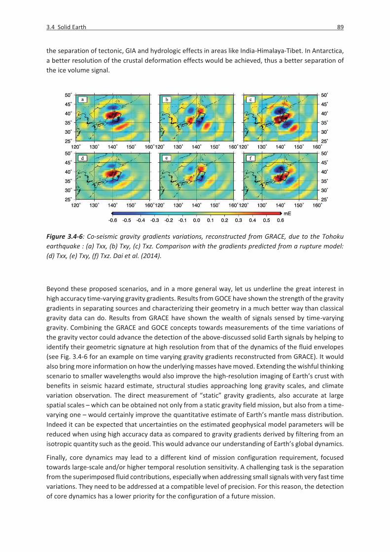
3.4 Solid Earth 89
the separation of tectonic, GIA and hydrologic effects in areas like India-Himalaya-Tibet. In Antarctica, a better resolution of the crustal deformation effects would be achieved, thus a better separation of the ice volume signal.
Figure 3.4-6: Co-seismic gravity gradients variations, reconstructed from GRACE, due to the Tohoku earthquake : (a) Txx, (b) Txy, (c) Txz. Comparison with the gradients predicted from a rupture model: (d) Txx, (e) Txy, (f) Txz. Dai et al. (2014).
Beyond these proposed scenarios, and in a more general way, let us underline the great interest in high accuracy time-varying gravity gradients. Results from GOCE have shown the strength of the gravity gradients in separating sources and characterizing their geometry in a much better way than classical gravity data can do. Results from GRACE have shown the wealth of signals sensed by time-varying gravity. Combining the GRACE and GOCE concepts towards measurements of the time variations of the gravity vector could advance the detection of the above-discussed solid Earth signals by helping to identify their geometric signature at high resolution from that of the dynamics of the fluid envelopes (see Fig. 3.4-6 for an example on time varying gravity gradients reconstructed from GRACE). It would also bring more information on how the underlying masses have moved. Extending the wishful thinking scenario to smaller wavelengths would also improve the high-resolution imaging of Earth’s crust with benefits in seismic hazard estimate, structural studies approaching long gravity scales, and climate variation observation. The direct measurement of “static” gravity gradients, also accurate at large spatial scales – which can be obtained not only from a static gravity field mission, but also from a time-varying one – would certainly improve the quantitative estimate of Earth’s mantle mass distribution. Indeed it can be expected that uncertainties on the estimated geophysical model parameters will be reduced when using high accuracy data as compared to gravity gradients derived by filtering from an isotropic quantity such as the geoid. This would advance our understanding of Earth’s global dynamics.
Finally, core dynamics may lead to a different kind of mission configuration requirement, focused towards large-scale and/or higher temporal resolution sensitivity. A challenging task is the separation from the superimposed fluid contributions, especially when addressing small signals with very fast time variations. They need to be addressed at a compatible level of precision. For this reason, the detection of core dynamics has a lower priority for the configuration of a future mission.

90 3 Derivation of requirements for main thematic fields
Figure 3.4-7: Expected signals for different phenomena in comparison to the error curves of five mission scenarios and the GRACE error curve. Distinction is made between gravity and gravity variation rates.
3.4.7 Definition of theme-specific science requirement
The main themes in solid Earth scientific research and societal applications that require a next generation gravity mission are the following: 1) Monitoring Earth’s tectonic activity, 2) Evolution of Earth crust due to GIA and plate movements, 3) Management of natural resources, and 4) Overarching 4D mantle and core evolution and influence on Earth evolution. Figure 3.4-8 summarizes these themes and their temporal and spatial resolution. These main themes require different improvements from a future generation satellite mission, in terms of enhanced spatial resolution, higher precision at long wavelengths, longer time series and improved temporal resolution.
Figure 3.4-8: Main themes in solid Earth and relation to wavelengths and time variations.

3.4 Solid Earth 91
Setting as priority for societal needs the first two themes, which aim to improve natural hazard monitoring and climate change, the most important requirement for a next generation gravity mission is an increase in spatial resolution. A spatial resolution of 200 km with an accuracy of 0.5 μGal (as provided by scenario 2) would allow to detect tectonic activity equivalent to magnitude 7 events, including seismic and aseismic, creeping movement. This would considerably increase the number of events that could be monitored, as shown in Fig. 3.4-9. For the time interval 1900-2014 a threshold of M> 8.5 sees 0.14 events/year, of M> 7.8 sees 1 event/year, and of M> 7 gives a leap to 12 events/yr. For crustal evolution monitoring it would allow to distinguish tectonic movement from GIA signal, allowing to approach scales of single orogens. Including gravity data of such a high quality will significantly enhance the areas that can be investigated and distinguish a local from a global hazard. Identification of long-term effects and the separation from annual to interannual climatic factors which affect surface deformation of the crust, time series length of at least 30 years is required. These long time series provided with a trend accuracy of 0.05 μGal/yr on scales of 200 km will be sufficient for the first time to provide estimates of mass movements at topography, at ocean bottom and at regional scale, and at the lower crust. As a novel application it is planned to distinguish the creeping crust at subduction zones from a locked zone, which is crucial for hazard estimation of the interseismic interval of large earthquakes. Even though temporal resolution is considered less important (compared to spatial resolution), mass earthquake monitoring profits from an improved time resolution (for instance weekly) to distinguish the instant effects from the long-term movements. An example is the coseismic effect on mass redistribution as distinguished from the following postseismic effect.
Figure 3.4-9: Number of earthquakes with magnitude greater 6. Worldwide for the time interval 1900-2014 (NEIC Database).
92 3 Derivation of requirements for main thematic fields
In order to meet the societal challenges identified in Sections 3.4.1 and 3.4.5, the following threshold and target requirements can be identified:
1) Monitoring Earth tectonic activity: Improved spatial resolution increases the number of faults that can be monitored with an exponential proportionality factor. Scenario 2 would allow to monitor M > 7 earthquakes, amounting to 12 events/year. Scenario 1 would allow to monitor events with M > 7.8, amounting to 1 event/year. (With GRACE only events with M> 8.5 can be monitored, amounting to 0.14 events/year). Monthly resolution is required, daily to weekly data is vital for short-term monitoring. With daily resolution and longer wavelength recovery 400-800 km, the threshold magnitude would be larger but still smaller than M = 8.0. With daily resolution, postseismic transient gravity change may be observed, which may be useful to discriminate various processes, including others than seismic signals. Conversely, for other studies such as oceanography, undersea earthquake signals should be removed from the GRACE data.
� Threshold: Scenario 1 � Target: Scenario 2 � Wishful thinking: 1 mGal@10km
2) Evolution of Earth crust due to GIA and plate movement: Spatial and temporal resolution are less critical with respect to Earth’s tectonic activity. Monthly resolution is adequate. As long term effects are involved, the most important aspect is a continuous time series in combination with an increased spatial resolution. The minimum required time series is 6 years.
� Threshold: Scenario 1 in continuity with GRACE follow on. � Target: Scenario 2 ; 1 cm EWH/yr@200 km; � Wishful thinking: 1 microGal/year@100 km; 0.02 EWH/yr@100 km wishful thinking for GIA
is a long time series of decades which allows perfect separation of climatic signals from GIA.
3) Management of natural resources: improved spatial resolution is important for the static part of the problem. High temporal resolution is necessary for monitoring of underground anthropogenically driven mass variations. Monthly resolution is adequate, weekly resolution is desirable.
� Threshold: Scenario 1 � Target: Scenario 2 � Wishful thinking: 1 mGal@10 km
4) Overarching 4D Earth model: key constraints are satellite observations on the widest spectrum of wavelengths imaginable and with as much temporal resolution as possible.
� Threshold: Scenario 1 � Target: Scenario 2 � Wishful thinking: daily resolution and wide spectrum from lowest to crustal scale (10 km)
wavelengths.

3.5 Cross-theme aspects and additional thematic fields 93
3.5 Cross-theme aspects and additional thematic fields In this section we summarize aspects which are at the interface of different themes and thus can only be resolved when considering the individual Earth’s components as one consistent system. It shall be considered rather as an exemplary collection than an exhaustive list. Further, additional thematic fields which can stongly benefit from future gravity field missions are addressed.
a) Global Isostatic Adjustment (GIA)
Long-term mass variations due to GIA overprint hydrological and cryospheric signals on different time scales and spatial resolutions. Typical regions with significant GIA signal are, for example, Antarctica, North America, and Fennoscandia. Continuous and higher accurate satellite gravimetry observations will give better constrains on GIA modeling. After removing long-term GIA-induced mass variations accurately, we gain an improved understanding of hydrological and cryospheric signals and their potential response to climate changes. In addition, increased spatial resolution and accuracy of new satellite gravimetry will reduce the uncertainties of GIA in places where the magnitude of GIA signal is debated now and is under the accuracy of current GRACE observations (such as Tibet). Better understanding GIA signal in these areas will allow us to retrieve more clearly hydrological and cryospheric mass variations on inter-annual, decadal and long-term time scales. Vice versa, after separation of surface mass effects from the GIA signal, an improved understanding of surface loading, the visco-elastic response, and ultimately about Earth’s rheology can be gained.
b) Sea level
Changes in continental water storage, mass changes of ice sheets and glaciers, deformations of the seafloor due to long-term GIA deformations and instantaneous elastic load deformations, displacements of gravity equipotential surfaces following mass redistributions – all these effects are integrated in eustatic sea level change. At the same time, climate variability and climate change cause steric sea level changes and ocean circulation changes. Satellite gravity has allowed to separate eustatic effects from steric effects in the total sea level changes observed by satellite altimetry. Moreover, sea level changes of particular origin (e.g. from ice mass loss in a particular region) exhibit distinct patterns – sea level fingerprints – controlled by the sea level equation. Geodetic observations therefore have the potential to separate, by observing purely oceanic patterns, the origins of sea level change. However, sea level fingerprints are particularly pronounced in coastal regions, where the resolution limits of GRACE inhibit their separation from continental mass changes. There, a higher-resolution mission can allow significant progress. Coastal regions are also those regions that determine human vulnerability to sea level changes. Again, higher-resolution satellite gravity will help to assess and to understand the nature of those changes. c) Atmosphere
Atmosphere models are currently used in gravity field processing as external information, mainly for reducing short-period mass variations with periods which cannot be temporally resolved by current satellite gravity mission. Correspondingly, errors in these atmospheric models cause temporal aliasing effects such as the typical GRACE striping errors in the gravity field. However, as gravity missions measure the sum of all masses/mass variations, they sense also atmospheric signals. Provided a higher temporal resolution and accuracy of a future gravity field mission, atmospheric parameters derived from gravity field satellites could be fed into atmospheric models, thus help improving the model

94 3 Derivation of requirements for main thematic fields
quality in an iterative feed-back loop. Additionally, in contrast to standard GRACE processing approaches currently it is attempted to avoid de-aliasing by reducing atmospheric (and ocean) signals as a pre-processing step, but rather to estimate the full time-variable signal with high temporal resolution, which also contains atmospheric mass variations. By this, a future gravity field mission constellation could set the grounds for a new and strongly improved processing logic. The potential and added value for atmospheric modelling and the impact on medium-term weather forecast and climate modelling still needs to be assessed.
d) Geodesy – height systems
Globally, more than 100 national and regional height systems exist, which refer to a local datum realized by a single tide gauge measuring the local mean sea level. As an example, large differences between the two official vertical datums of Canada (CGVD28) and the USA (NAVD88) exist, and constitute a significant problem for many engineering projects in areas along the Canadian and USA border.
An equipotential surface defined by the gravity field, the geoid, defines a physical reference surface and correspondingly an ideal zero-height surface. The availability of global gravity information from gravity field satellites, complemented by terrestrial and air-borne gravity to add the high-frequency signal content which cannot be resolved by satellite techniques, allows measuring heights by a combination of quite inexpensive GNSS measurements and the precise knowledge of the gravity field over the continents, a method which is usually called “GNSS-levelling” (Featherstone and Filmer 2012). The technique of GNSS-levelling can be applied for the connection and unification of national height systems in continental areas and in combination with satellite altimetry, which provides ellipsoidal heights over the oceans, even height systems across the oceans can be connected. Fig. 3.5-1 shows a schematic view of the principle of global height system unification with GOCE. National height systems (vertical reference systems – VRS) are usually connected to local tide gauges, which are not on the same equipotential surface and thus define “national” zero levels. Heights are transferred to the inland via spirit levelling. By determining the deviation of the individual VRS’s (�A, �B) from the globally consistent high-resolution geoid acting as an ideal “zero surface”, the national height systems can be connected.
Figure 3.5-1: Schematic view on the principle of global height system unification.
3.5 Cross-theme aspects and additional thematic fields 95
GNSS-levelling has also a high economic potential, because it can replace the expensive and time consuming spirit levelling. GNSS-levelling specifically is of great interest for countries with a less advanced geodetic infrastructure like primary reference stations, positioning and levelling networks, and terrestrial gravity data. There are many developing and newly industrializing countries lacking any vertical reference system at all (Rummel 2013), a situation which creates major negative consequences for construction, infrastructure and the potential for industrialization.
One of the main problems is the spectral limitation of satellite gravity field missions, resulting in omission errors, i.e. non-resolved gravity signals, which can amount to high-frequency geoid height signals of several decimetres in mountainous regions. A future mission with a performance of Scenario 2 will be able to reduce the omission error to only a few centimeters, even in regions where no or only low-quality terrestrial gravity data are available. Beyond the provision of high-resolution static gravity field information, a future satellite gravity constellations could provide also temporal changes in the geoid and correspondingly of heights. This is particularly important in regions with strong gravity trends, e.g. due to GIA signals, and contributes to a correct description of regional relative sea level changes. e) Thermosphere density and wind
The instrumentation and orbital characteristics of the past gravity field missions CHAMP, GRACE and GOCE have proven to be especially well suited for the derivation of data sets of upper atmospheric air density and crosswind speed at the altitude of these satellites. These data sets have been derived from an aerodynamic analysis of the observed satellite accelerations (Bruinsma et al. 2004, Doornbos et al. 2010 and references therein). The thermosphere data sets from these missions continue to have a large impact on research of the dynamics of the neutral upper atmosphere and its relation with solar activity as well as with upwards propagating waves from the lower atmosphere, and coupling with ionospheric and magnetospheric processes. Continuing and improving the measurement and data processing of accelerometer-derived thermospheric density and crosswind speeds with future gravity missions would be of great benefit to these science disciplines and significantly increase the science return from these missions.
A simple extension of the current data sets over even longer time periods will already provide important additional scientific benefits. For example, additional data is required for a better separation of seasonal, local solar time, longitudinal and solar activity variations in the structure and dynamics of the thermosphere (e.g. Lieberman et al. 2013). In addition, the future availability of density data, spanning multiple decades, will allow for a very detailed investigation of long-term cooling of the upper atmosphere, which is thought to be partly caused by the increase of greenhouse gases in the lower layers of the atmosphere (Emmert et al. 2008). The interaction between neutral atmospheric particles and charged particles means that long-term changes in the Earth’s magnetic field might play a role in long term change processes as well. The separation of such changes from changes introduced by variability of the solar energy input requires the availability of accurate observation data on thermospheric densities over multiple 11-year solar cycles, starting in 2000 with CHAMP and extending beyond the operation period of GRACE Follow-on.
Simultaneous observations from a multi-satellite mission in multiple orbital planes separated in right ascension of the nodes (and therefore in local time) will allow for better observations of transient phenomena in the upper atmosphere, such as travelling atmospheric disturbances, as well as better separation of local time and seasonal variations. If one of the orbital planes has a relatively low inclination, the crosswind measurements will be able to provide unique information on meridional winds at lower latitudes. Additional instrumentation, such as a neutral mass spectrometer for

96 3 Derivation of requirements for main thematic fields
determining the composition, temperature and/or wind speed, would provide great synergy with acceleration-derived data, and be of enormous benefit for upper atmospheric research. The additional data would provide the means to accurately determine the absolute scale of thermospheric density (Doornbos et al. 2013).

97
4. Consolidated Science Requirements Based on the science and user requirements derived by the individual thematic fields, i.e., continental hydrology, cryosphere, ocean and solid Earth (Chapter 3), joint requirements for a future satellite gravity mission constellation have been derived. Naturally, the individual requirements differ in the various fields and even among different applications within one field. Therefore, the following joint requirements shall be interpreted as a compromise for a mission configuration which is able to cover a wide range of applications, but which could be optimized further for a specific discipline. In general, the conclusion in all four fields is that, apart from the extension of the currently available time series of global gravity measurements, which improves particularly trend estimates and thus the separability of natural and antropogenically induced effects of climate change, an increase of spatial resolution is given priority over an increase of temporal resolution. Therefore, the joint product needs first are given as performance numbers of monthly fields. The performance of sub-monthly down to daily resolution are derived from the monthly scenarios, because they can be simultaneously realized through mission design by appropriate choice of sub-cycles, or additional satellite pairs. A future mission is on the one hand driven by science needs and novel science opportunities, but must on the other hand also serve a significant number of applications with societal benefit. Therefore, gravity field products on short time-scales of 1 to a few days and their availability with short latencies are also required. In the following, the consolidated science and user needs are given as threshold and target requirements following the definition in chapter 3. a) Threshold requirements The threshold values for a future satellite gravity mission constellation are2:
Spatial resolution
Equivalent Water Height Geoid Monthly field Long-term trend Monthly field Long-term trend
400 km 200 km 150 km 100 km
5 mm 10 cm 50 cm
5 m
0.5 mm/yr 1 cm/yr 5 cm/yr 0.5 m/yr
50 μm 0.5 mm 1 mm
10 mm
5 μm/yr 0.05 mm/yr 0.1 mm/yr 1 mm/yr
2 For the sake of lucidity, the numbers are given only as equivalent water heights and geoid heights. The respective numbers for other gravity field functionals can be derived from Tables 1-1 and A-1.

98 4 Consolidated Science Requirements
Referring to the scientific and societal challenges identified in Fig. 1-1, the benefits of a mission with such a specification are (not exhaustive):
Scientific challenges Closure of global water and regional water balances
� Water storage in medium-scale river basins � Derivation of long-term storage trends � Understanding climate change impacts on the water cycle � Assessing the human impact on the water cycle
Dynamics of ice sheets and glaciers
� Mass balance of major ice sheet drainage basins in Greenland and Antarctica and of large glacier clusters
� Cryosphere contribution to global and regional sea level Flux exchange between land and atmosphere
� Determination of atmospheric mass variations � In-situ observation of atmospheric density as input to
atmospheric models Ocean mass and heat transport budget
� Improved determination of Mean Dynamic Topography � Improved determination of ocean bottom pressure and deep
ocean flow, in particular AMOC Sea level rise � Global to regional sea level estimates
� Improved separation of mass and steric contributions to sea level
Solid Earth dynamics � Monitoring the mass shifts due to earthquake events with magnitude M ≥ 7.8 (about 1 event per year)
� Monitoring of large tectonic movements in restricted areas � Monitoring of underground anthropogenically driven mass
variations Separation of natural and anthropogenic processes
� Separation of anthropogenic and natural effects on large spatial scales
Societal challenges Water management and ground water monitoring
� Significant contribution to applications of water management on medium to large scale
Monitoring and forecasting of floods and droughts
� Early warning for extreme events, such as floods and droughts
Climate impact of water cycle and ice sheets
� Contribution to separation of anthropogenic and natural effects on large spatial scales
� Contributions to near-future climate predictions Coastal vulnerability � Global to regional sea level estimates
� Improved separation of mass and steric contributions to sea level
Height systems and land management
� Monitoring of large to medium scale changes in global height reference surface
Risk assessment of natural hazards
� Risk management related to natural hazards
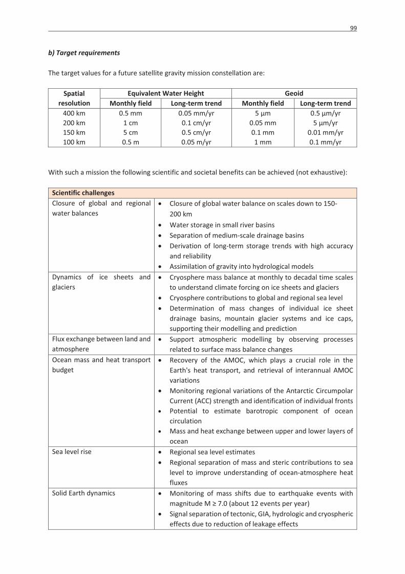
99
b) Target requirements The target values for a future satellite gravity mission constellation are:
Spatial resolution
Equivalent Water Height Geoid Monthly field Long-term trend Monthly field Long-term trend
400 km 200 km 150 km 100 km
0.5 mm 1 cm 5 cm 0.5 m
0.05 mm/yr 0.1 cm/yr 0.5 cm/yr 0.05 m/yr
5 μm 0.05 mm 0.1 mm 1 mm
0.5 μm/yr 5 μm/yr
0.01 mm/yr 0.1 mm/yr
With such a mission the following scientific and societal benefits can be achieved (not exhaustive):
Scientific challenges Closure of global and regional water balances
� Closure of global water balance on scales down to 150-200 km
� Water storage in small river basins � Separation of medium-scale drainage basins � Derivation of long-term storage trends with high accuracy
and reliability � Assimilation of gravity into hydrological models
Dynamics of ice sheets and glaciers
� Cryosphere mass balance at monthly to decadal time scales to understand climate forcing on ice sheets and glaciers
� Cryosphere contributions to global and regional sea level � Determination of mass changes of individual ice sheet
drainage basins, mountain glacier systems and ice caps, supporting their modelling and prediction
Flux exchange between land and atmosphere
� Support atmospheric modelling by observing processes related to surface mass balance changes
Ocean mass and heat transport budget
� Recovery of the AMOC, which plays a crucial role in the Earth's heat transport, and retrieval of interannual AMOC variations
� Monitoring regional variations of the Antarctic Circumpolar Current (ACC) strength and identification of individual fronts
� Potential to estimate barotropic component of ocean circulation
� Mass and heat exchange between upper and lower layers of ocean
Sea level rise � Regional sea level estimates � Regional separation of mass and steric contributions to sea
level to improve understanding of ocean-atmosphere heat fluxes
Solid Earth dynamics � Monitoring of mass shifts due to earthquake events with magnitude M ≥ 7.0 (about 12 events per year)
� Signal separation of tectonic, GIA, hydrologic and cryospheric effects due to reduction of leakage effects
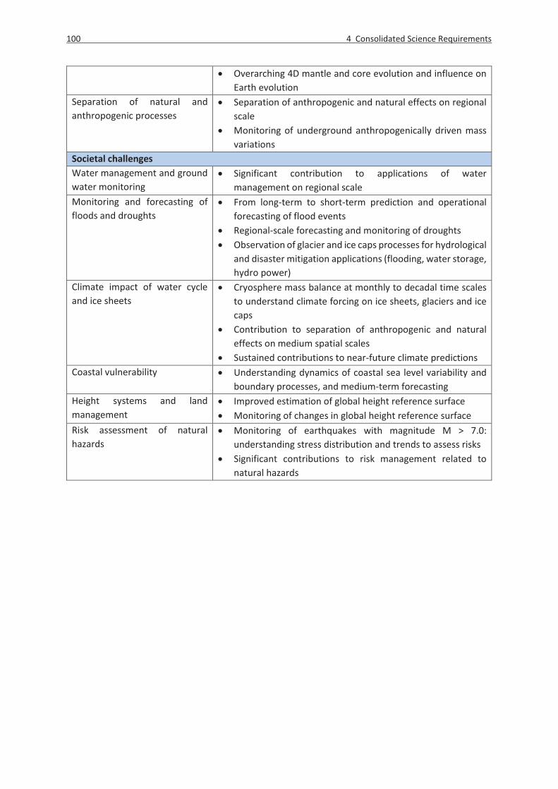
100 4 Consolidated Science Requirements
� Overarching 4D mantle and core evolution and influence on Earth evolution
Separation of natural and anthropogenic processes
� Separation of anthropogenic and natural effects on regional scale
� Monitoring of underground anthropogenically driven mass variations
Societal challenges Water management and ground water monitoring
� Significant contribution to applications of water management on regional scale
Monitoring and forecasting of floods and droughts
� From long-term to short-term prediction and operational forecasting of flood events
� Regional-scale forecasting and monitoring of droughts � Observation of glacier and ice caps processes for hydrological
and disaster mitigation applications (flooding, water storage, hydro power)
Climate impact of water cycle and ice sheets
� Cryosphere mass balance at monthly to decadal time scales to understand climate forcing on ice sheets, glaciers and ice caps
� Contribution to separation of anthropogenic and natural effects on medium spatial scales
� Sustained contributions to near-future climate predictions Coastal vulnerability � Understanding dynamics of coastal sea level variability and
boundary processes, and medium-term forecasting Height systems and land management
� Improved estimation of global height reference surface � Monitoring of changes in global height reference surface
Risk assessment of natural hazards
� Monitoring of earthquakes with magnitude M > 7.0: understanding stress distribution and trends to assess risks
� Significant contributions to risk management related to natural hazards

5.1 Continental Hydrology (chapter 3.1) 101
5. Bibliography 5.1 Continental Hydrology (chapter 3.1)
Alkama, R., and Coauthors (2010): Global Evaluation of the ISBA-TRIP Continental Hydrological System. Part I: Comparison to GRACE Terrestrial Water Storage Estimates and In Situ River Discharges. J. Hydrometeor, 11, 583–600.doi: http://dx.doi.org/10.1175/2010JHM1211.1
Awange, J. L., Forootan, E., Kusche, J., Kiema, J. B. K., Omondi, P. A., Heck, B., ... & Goncalves, R. M. (2013). Understanding the decline of water storage across the Ramser-Lake Naivasha using satellite-based methods. Advances in Water Resources, 60, 7-23.
Becker, M., William LLovel, Anny Cazenave, Andreas Güntner, Jean-François Crétaux (2010) Recent hydrological behavior of the East African great lakes region inferred from GRACE, satellite altimetry and rainfall observations, Comptes Rendus Geoscience, Volume 342, Issue 3, Pages 223-233, ISSN 1631-0713, http://dx.doi.org/10.1016/j.crte.2009.12.010.
Becker, M., Meyssignac, B., Xavier, L., Cazenave, A., Alkama, R., & Decharme, B. (2011). Past terrestrial water storage (1980–2008) in the Amazon Basin reconstructed from GRACE and in situ river gauging data. Hydrology and Earth System Sciences, 15(2), 533–546. doi:10.5194/hess-15-533-2011
Blöschl, G. and Sivapalan, M. (1995): Scale issues in hydrological modeling: a review. Hydrological Processes, Vol. 9, 251-290
Chen, J. L., Wilson, C. R., Tapley, B. D., Longuevergne, L., Yang, Z. L., & Scanlon, B. R. (2010a). Recent La Plata basin drought conditions observed by satellite gravimetry. Journal of Geophysical Research: Atmospheres (1984–2012), 115(D22).
Chen, J. L., Wilson, C. R., & Tapley, B. D. (2010b). The 2009 exceptional Amazon flood and interannual terrestrial water storage change observed by GRACE. Water Resources Research, 46(12)
Chen, Y., Velicogna, I., Famiglietti, J.S., Randerson, J.T. (2013). Satellite observations of terrestrial water storage provide early warning information about drought and fire season severity in the Amazon. Journal of Geophysical Research: Biogeosciences 118, doi:10.1002/jgrg.20046.
Crowley, J. W., J. X. Mitrovica, R. C. Bailey, M. E. Tamisiea, and J. L. Davis (2006), Land water storage within the Congo Basin inferred from GRACE satellite gravity data, Geophys. Res. Lett., 33, L19402, doi:10.1029/2006GL027070.
Dill, R. (2008), Hydrological model LSDM for operational Earth rotation and gravity field variations Scientific Technical Report 08/09, pp. 37, GFZ Potsdam, Germany, doi:10.2312/GFZ.b103-08095.
Dobslaw, H. Bergmann-Wolf, I., Dill, R., Forootan, E., Klemann, V., Kusche, J., Sasgen, I. (2015), The updated ESA Earth System Model for future gravity mission simulation studies, J. Geodesy, doi:10.1007/s00190-014-0787-8.
Döll, P., Müller Schmied, H., Schuh, C., Portmann, F. T., & Eicker, A. (2014a). Global-scale assessment of groundwater depletion and related groundwater abstractions: Combining hydrological modeling with information from well observations and GRACE satellites. Water Resources Research, 50(7), 5698-5720.
Döll, P., Fritsche, M., Eicker, A., Müller Schmied, H. (2014b): Seasonal water storage variations as impacted by water abstractions: Comparing the output of a global hydrological model with GRACE and GPS observations. Survey in Geophysics. 35 (6), 1311-1331, doi: 10.1007/s10712-014-9282-2
Douville, H., Ribes, A., Decharme, B., Alkama, R., & Sheffield, J. (2013). Anthropogenic influence on multidecadal changes in reconstructed global evapotranspiration. Nature Climate Change, 3(1), 59-62.
Eicker, A., Schumacher, M., Kusche, J., Döll, P., Müller Schmied, H. (2014) Calibration/Data Assimilation Approach for Integrating GRACE Data into the WaterGAP Global Hydrology Model (WGHM) Using an Ensemble Kalman Filter: First Results, Surveys in Geophysics, Volume 35, Issue 6, pp 1285-1309, doi: 10.1007/s10712-014-9309-8

102 5 Bibliography
Espinoza J.C., Ronchail J., Frappart F., Lavado W., Santini W., Guyot J-L. (2013). The major floods in the Amazonas River and tributaries (Western Amazon basin) during the 1970 - 2012 period: A focus on the 2012 flood, Journal of Hydrometeorology, 14, 1000-1008, doi: 10.1175/JHM-D-12-0100.1.
Famiglietti, J. S., Lo, M., Ho, S. L., Bethune, J., Anderson, K. J., Syed, T. H., ... & Rodell, M. (2011). Satellites measure recent rates of groundwater depletion in California's Central Valley. Geophysical Research Letters, 38(3).
Famiglietti, J. S., & Rodell, M. (2013). Water in the Balance.Science, 340(6138), 1300-1301.
Feng, W., M. Zhong, J.-M.Lemoine, R. Biancale, H.-T. Hsu, and J. Xia (2013), Evaluation of groundwater depletion in North China using the Gravity Recovery and Climate Experiment (GRACE) data and ground-based measurements, Water Resour. Res., 49, 2110–2118, doi:10.1002/wrcr.20192.
Fersch, B., Kunstmann, H., Bárdossy, A., Devaraju, B., Sneeuw N. (2012): Continental-Scale Basin Water Storage Variation from Global and Dynamically Downscaled Atmospheric Water Budgets in Comparison with GRACE-Derived Observations. J. Hydrometeor, 13, 1589–1603.doi: http://dx.doi.org/10.1175/JHM-D-11-0143.1
Forootan; E., R. Rietbroek; J. Kusche; M.A. Sharifi; J. Awange; M. Schmidt; P. Omondi; J. Famiglietti (2014a). Separation of large scale water storage patterns over Iran using GRACE, altimetry and hydrological data. Journal of Remote Sensing of Environment, 140, Pages 580-595, dx.doi.org/10.1016/j.rse.2013.09.025
Forootan; E., J. Kusche; I. Loth; W-D. Schuh; A. Eicker; J. Awange; L. Longuevergne; B. Diekkrueger; M. Schmidt; C.K. Shum (2014b). Multivariate prediction of total water storage anomalies over West Africa from multi-satellite data. Surveys in Geophysics, in-press, doi:10.1007/s10712-014-9292-0.
Frappart, F., Papa, F., Da Silva, J. S., Ramillien, G., Prigent, C., Seyler, F., & Calmant, S. (2012).Surface freshwater storage and dynamics in the Amazon basin during the 2005 exceptional drought.Environmental Research Letters, 7(4), 044010.
Gao, H., Tang, Q., Ferguson, C. R., Wood, E. F., & Lettenmaier, D. P. (2010). Estimating the water budget of major US river basins via remote sensing. International Journal of Remote Sensing, 31(14), 3955-3978.
García-García, D., Caroline C. Ummenhofer, Victor Zlotnicki (2011) Australian water mass variations from GRACE data linked to Indo-Pacific climate variability, Remote Sensing of Environment, Volume 115, Issue 9, Pages 2175-2183, ISSN 0034-4257, http://dx.doi.org/10.1016/j.rse.2011.04.007
Gerten, D., Lucht, W., Ostberg, S., Heinke, J., Kowarsch, M., Kreft, H., ... & Schellnhuber, H. J. (2013). Asynchronous exposure to global warming: freshwater resources and terrestrial ecosystems. Environmental Research Letters, 8(3), 034032.
Goddard, L., Kumar, A., Solomon, A., Smith, D., Boer, G., Gonzalez, P., …, Delworth, T. (2013). A verification framework for interannual-to-decadal predictions experiments. Climate Dynamics, 245272.doi:10.1007/s00382-012-1481-2
Gonçalvès, J., J. Petersen, P. Deschamps, B. Hamelin, and O. Baba-Sy (2013), Quantifying the modern recharge of the “fossil” Sahara aquifers, Geophys. Res. Lett., 40, 2673–2678, doi:10.1002/grl.50478.
Grippa, M., Kergoat, L., Frappart, F., Araud, Q., Boone, A., De Rosnay, P., ...& Ramillien, G. (2011). Land water storage variability over West Africa estimated by Gravity Recovery and Climate Experiment (GRACE) and land surface models. Water Resources Research, 47(5).
Güntner, A. (2008). Improvement of global hydrological models using GRACE data. Surveys in geophysics, 29(4-5), 375-397.
Han, S.-C., H. Kim, I.-Y. Yeo, P. Yeh, T. Oki, K.-W. Seo, D. Alsdorf, and S. B. Luthcke (2009), Dynamics of surface water storage in the Amazon inferred from measurements of inter-satellite distance change, Geophys. Res. Lett., 36, L09403, doi: 10.1029/2009GL037910.
Houborg, R., M. Rodell, B. Li, R. Reichle, and B. Zaitchik (2012) Drought indicators based on model assimilated GRACE terrestrial water storage observations, Wat. Resour. Res., 48, W07525, doi:10.1029/2011WR011291.
Jensen, L., R. Rietbroek, and J. Kusche (2013), Land water contribution to sea level from GRACE and Jason-1 measurements, J. Geophys. Res. Oceans, 118, 212–226, doi:10.1002/jgrc.20058.
Joodaki, G., J. Wahr, and S. Swenson (2014), Estimating the human contribution to groundwater depletion in the Middle East, from GRACE data, land surface models, and well observations, Water Resour. Res., 50, 2679–2692, doi:10.1002/2013WR014633.
5.1 Continental Hydrology (chapter 3.1) 103
Jung, M., Reichstein, M., Ciais, P., Seneviratne, S. I., Sheffield, J., Goulden, M. L., ... & Zhang, K. (2010). Recent decline in the global land evapotranspiration trend due to limited moisture supply. Nature, 467(7318), 951-954.
Kim, H., P. J.-F. Yeh, T. Oki, and S. Kanae (2009), Role of rivers in the seasonal variations of terrestrial water storage over global basins, Geophys. Res. Lett., 36, L17402, doi:10.1029/2009GL039006.
Klees, R., Zapreeva, E. A., Winsemius, H. C., and Savenije, H. H. G. (2006) The bias in GRACE estimates of continental water storage variations, Hydrol. Earth Syst. Sci. Discuss., 3, 3557-3594, doi:10.5194/hessd-3-3557-2006
Leblanc, M., Sarah Tweed, Albert Van Dijk, Bertrand Timbal (2012) A review of historic and future hydrological changes in the Murray-Darling Basin, Global and Planetary Change, Volumes 80–81, Pages 226-246, ISSN 0921-8181, http://dx.doi.org/10.1016/j.gloplacha.2011.10.012.
Lehner, B., Grill G. (2013): Global river hydrography and network routing: baseline data and new approaches to study the world’s large river systems. Hydrological Processes, 27(15): 2171–2186.
Lettenmaier, D. P., & Famiglietti, J. S. (2006). Hydrology: Water from on high. Nature, 444(7119), 562-563.
Li, B., Rodell, M., Zaitchik, B.F., Reichle, R.H., Koster, R.D., van Dam, T.M. (2012): Assimilation of GRACE terrestrial water storage into a land surface model: evaluation and potentialvalue for drought monitoring in western and central Europe. Journal of Hydrology
Livneh, B. and Lettenmaier, D. P. (2012): Multi-criteria parameter estimation for the Unified Land Model, Hydrol. Earth Syst. Sci., 16, 3029-3048, doi:10.5194/hess-16-3029-2012.
Llovel, W., Becker, M., Cazenave, A., Crétaux, J.-F., & Ramillien, G. (2010). Global land water storage change from GRACE over 2002–2009; Inference on sea level. Comptes Rendus Geoscience, 342(3), 179–188. doi:10.1016/j.crte.2009.12.004
Lo, M.-H., J. S. Famiglietti, P. J.-F. Yeh, and T. H. Syed (2010), Improving parameter estimation and water table depth simulation in a land surface model using GRACE water storage and estimated base flow data, Water Resour. Res., 46, W05517, doi:10.1029/2009WR007855.
Long, D., Scanlon, B. R., Longuevergne, L., Sun, A. Y., Fernando, D. N., & Save, H. (2013). GRACE satellite monitoring of large depletion in water storage in response to the 2011 drought in Texas. Geophysical Research Letters, 40(13), 3395-3401.
Long, D., L. Longuevergne, and B. R. Scanlon (2014a), Uncertainty in evapotranspiration from land surface modeling, remote sensing, and GRACE satellites, Water Resour. Res., 50, 1131–1151, doi:10.1002/2013WR014581.
Long, D., Shen, Y., Sun, A., Hong, Y., Longuevergne, L., Yang, Y., ... & Chen, L. (2014b). Drought and flood monitoring for a large karst plateau in Southwest China using extended GRACE data. Remote Sensing of Environment, 155, 145-160.
Longuevergne, L., Scanlon, B. R., & Wilson, C. R. (2010). GRACE Hydrological estimates for small basins: Evaluating processing approaches on the High Plains Aquifer, USA. Water Resources Research, 46(11).
Longuevergne, L., Wilson, C. R., Scanlon, B. R., & Crétaux, J. F. (2012). GRACE water storage estimates for the Middle East and other regions with significant reservoir and lake storage. Hydrology & Earth System Sciences Discussions, 9(10).
Lorenz, C., Kunstmann, H., Devaraju, B., Tourian, M., Sneeuw, N., Riegger, J. (2014) Large-scale runoff from landmasses: a global assessment of the closure of the hydrological and atmospheric water balances, Journal of Hydrometeorology, doi: 10.1175/JHM-D-13-0157.1
Meehl, G., Goddard, L., Murphy, J., Stouffer, R. J., Boer, G., Danabasoglu, G., Stockdale, T. (2009). Decadal Prediction: Can it be skillful? Bull. A. Met. Soc., 90(10), 1467-1485.
Morishita, Y., Kosuke Heki (2008) Characteristic precipitation patterns of El Niño/La Niña in time-variable gravity fields by GRACE, Earth and Planetary Science Letters, Volume 272, Issues 3–4, Pages 677-682, ISSN 0012-821X, http://dx.doi.org/10.1016/j.epsl.2008.06.003
Mulder, G., Olsthoorn, T. N., Al-Manmi, D. A. M. A., Schrama, E. J. O., & Smidt, E. H. (2014). Identifying water mass depletion in Northern Iraq observed by GRACE. Hydrology and Earth System Sciences Discussions, 11(10), 11533-11563.

104 5 Bibliography
Ngo-Duc, T., K. Laval, G. Ramillien, J. Polcher, and A. Cazenave (2007), Validation of the land water storage simulated by Organising Carbon and Hydrology in Dynamic Ecosystems (ORCHIDEE) with Gravity Recovery and Climate Experiment (GRACE) data, Water Resour. Res., 43, W04427, doi:10.1029/2006WR004941.
Pan, Ming, Alok K. Sahoo, Tara J. Troy, Raghuveer K. Vinukollu, Justin Sheffield, Eric F. Wood (2012): Multisource Estimation of Long-Term Terrestrial Water Budget for Major Global River Basins. J. Climate, 25, 3191–3206.doi: http://dx.doi.org/10.1175/JCLI-D-11-00300.1
Phillips, T., R. S. Nerem, B. Fox-Kemper, J. S. Famiglietti, and B. Rajagopalan (2012), The influence of ENSO on global terrestrial water storage using GRACE, Geophys. Res. Lett., 39, L16705, doi:10.1029/2012GL052495.
Pokhrel, Y. N., Y. Fan, G. Miguez-Macho, P. J.-F. Yeh, and S.-C. Han (2013), The role of groundwater in the Amazon water cycle: 3. Influence on terrestrial water storage computations and comparison with GRACE, J. Geophys. Res. Atmos., 118, 3233–3244, doi:10.1002/jgrd.50335.
Ramillien, G., Frappart, F., Güntner, A., Ngo-Duc, T., Cazenave, A., & Laval, K. (2006). Time variations of the regional evapotranspiration rate from Gravity Recovery and Climate Experiment (GRACE) satellite gravimetry. Water resources research, 42(10).
Reager, J. T., and J. S. Famiglietti (2009), Global terrestrial water storage capacity and flood potential using GRACE, Geophys. Res. Lett., 36, L23402, doi:10.1029/2009GL040826.
Reager, J. T., Thomas, B. F., & Famiglietti, J. S. (2014). River basin flood potential inferred using GRACE gravity observations at several months lead time. Nature Geoscience, 7(8), 588-592.
Rodell, M., .Velicogna, and J. S. Famiglietti (2009) Satellite-based estimates of groundwater depletion in India. Nature 460.7258: 999-1002.
Sahoo, A. K., Pan, M., Troy, T. J., Vinukollu, R. K., Sheffield, J., & Wood, E. F. (2011). Reconciling the global terrestrial water budget using satellite remote sensing. Remote Sensing of Environment, 115(8), 1850-1865.
Scanlon, B. R., Faunt, C. C., Longuevergne, L., Reedy, R. C., Alley, W. M., McGuire, V. L., & McMahon, P. B. (2012). Groundwater depletion and sustainability of irrigation in the US High Plains and Central Valley.Proceedings of the national academy of sciences, 109(24), 9320-9325.
Seitz, F., Schmidt, M., & Shum, C. K. (2008). Signals of extreme weather conditions in Central Europe in GRACE 4-D hydrological mass variations.Earth and Planetary Science Letters, 268(1), 165-170.
Seneviratne, S. I., Lüthi, D., Litschi, M., & Schär, C. (2006). Land–atmosphere coupling and climate change in Europe. Nature, 443(7108), 205-209.
Seo, K.-W., D. Ryu, B.-M. Kim, DE Waliser, B. Tian, and J. Eom (2010), GRACE and AMSR-E-based estimates of winter season solid precipitation accumulation in the Arctic drainageregion, J. Geophys. Res., 115, D20117, doi: 10.1029/2009JD013504.
Sheffield, J., C. R. Ferguson, T. J. Troy, E. F. Wood, and M. F. McCabe (2009), Closing the terrestrial water budget from satellite remote sensing, Geophys. Res. Lett., 36, L07403, doi:10.1029/2009GL037338.
Springer, A., Kusche, J., Hartung, K., Ohlwein, C., & Longuevergne, L. (2014). New estimates of variations in water flux and storage over Europe based on regional (Re) analyses and multisensor observations. Journal of Hydrometeorology, 15(6), 2397-2417.
Su, H., Z.-L.Yang, R. E. Dickinson, C. R. Wilson, and G.-Y. Niu (2010), Multisensor snow data assimilation at the continental scale: The value of Gravity Recovery and Climate Experiment terrestrial water storage information, J. Geophys. Res., 115, D10104, doi:10.1029/2009JD013035.
Swenson, S., and J. Wahr (2002) Methods for inferring regional surface-mass anomalies from Gravity Recovery and Climate Experiment (GRACE) measurements of time-variable gravity, J. Geophys. Res., 107(B9), 2193, doi:10.1029/2001JB000576
Swenson, S., J. Wahr (2006): Estimating Large-Scale Precipitation Minus Evapotranspiration from GRACE Satellite Gravity Measurements. J. Hydrometeor, 7, 252–270.doi: http://dx.doi.org/10.1175/JHM478.1
Swenson, S. (2010): Assessing High-Latitude Winter Precipitation from Global Precipitation Analyses Using GRACE. J. Hydrometeor, 11, 405–420.doi: http://dx.doi.org/10.1175/2009JHM1194.1
Syed, T. H., J. S. Famiglietti, V. Zlotnicki, and M. Rodell (2007), Contemporary estimates of Pan-Arctic freshwater discharge from GRACE and reanalysis, Geophys. Res. Lett., 34, L19404, doi:10.1029/2007GL031254.
5.1 Continental Hydrology (chapter 3.1) 105
Syed, T. H., Famiglietti, J. S., Rodell, M., Chen, J., & Wilson, C. R. (2008). Analysis of terrestrial water storage changes from GRACE and GLDAS. Water Resources Research, 44(2).
Syed, T. H., Famiglietti, J. S., Chambers, D. P., Willis, J. K., & Hilburn, K. (2010). Satellite-based global-ocean mass balance estimates of interannual variability and emerging trends in continental freshwater discharge. Proceedings of the National Academy of Sciences, 107(42), 17916-17921.
Tang, Qiuhong, Huilin Gao, Pat Yeh, Taikan Oki, Fengge Su, Dennis P. Lettenmaier (2010): Dynamics of Terrestrial Water Storage Change from Satellite and Surface Observations and Modeling. J. Hydrometeor, 11, 156–170.doi: http://dx.doi.org/10.1175/2009JHM1152.1
Taylor, R. G., Scanlon, B., Döll, P., Rodell, M., Van Beek, R., Wada, Y., ...& Treidel, H. (2013). Ground water and climate change. Nature Climate Change, 3(4), 322-329.
Tiwari, V. M., Wahr, J., and Swenson, S. (2009). Dwindling groundwater resources in northern India, from satellite gravity observations. Geophysical Research Letters, 36:18401–+, doi:10.1029/2009GL039401
Tourian, M. J., Elmi, O., Chen, Q., Devaraju, B., Roohi, S., & Sneeuw, N. (2015). A spaceborne multisensor approach to monitor the desiccation of Lake Urmia in Iran. Remote Sensing of Environment, 156, 349-360.
van Dijk, A. I. J. M., Renzullo, L. J., Wada, Y., and Tregoning, P. (2014): A global water cycle reanalysis (2003–2012) merging satellite gravimetry and altimetry observations with a hydrological multi-model ensemble, Hydrol. Earth Syst. Sci., 18, 2955-2973, doi:10.5194/hess-18-2955-2014.
Vergnes, J.-P.and Decharme, B. (2012): A simple groundwater scheme in the TRIP river routing model: global off-line evaluation against GRACE terrestrial water storage estimates and observed river discharges, Hydrol. Earth Syst. Sci., 16, 3889-3908, doi:10.5194/hess-16-3889-2012.
Voss, Katalyn A., et al. (2013) Groundwater depletion in the Middle East from GRACE with implications for transboundary water management in the Tigris-Euphrates-Western Iran region. Water resources research 49.2: 904-914.
Wada, Y., et al. (2013), Multimodel projections and uncertainties of irrigation water demand under climate change, Geophys. Res. Lett., 40, 4626–4632, doi:10.1002/grl.50686.
Wang, X., C. de Linage, J. Famiglietti, and C. S. Zender (2011), Gravity Recovery and Climate Experiment (GRACE) detection of water storage changes in the Three Gorges Reservoir of China and comparison with in situ measurements, Water Resour. Res., 47, W12502, doi:10.1029/2011WR010534.
Werth, S., Güntner, A. (2010): Calibration analysis for water storage variability of the globalhydrological model WGHM. Hydrology and Earth System Sciences 14(1), 59.
Xavier, L., M. Becker, A. Cazenave, L. Longuevergne, W. Llovel, O.C. Rotunno Filho (2010) Interannual variability in water storage over 2003–2008 in the Amazon Basin from GRACE space gravimetry, in situ river level and precipitation data, Remote Sensing of Environment, Volume 114, Issue 8, Pages 1629-1637, ISSN 0034-4257, http://dx.doi.org/10.1016/j.rse.2010.02.005.
Xie, H., Longuevergne, L., Ringler, C., and Scanlon, B. R. (2012): Calibration and evaluation of a semi-distributed watershed model of Sub-Saharan Africa using GRACE data, Hydrol. Earth Syst. Sci., 16, 3083-3099, doi:10.5194/hess-16-3083-2012.
Yang, Z.-L., G.-Y. Niu, K. E. Mitchell, F. Chen, M. B. Ek, M. Barlage, K. Manning, D. Niyogi, M. Tewari, and Y. Xia (2011), The community Noah land surface model with multiparameterization options (Noah-MP): 2. Evaluation over global river basins, J. Geophys. Res., doi:10.1029/2010JD015140
Yeh, P. J. F., Swenson, S. C., Famiglietti, J. S., & Rodell, M. (2006). Remote sensing of groundwater storage changes in Illinois using the Gravity Recovery and Climate Experiment (GRACE). Water Resources Research, 42(12).
Zaitchik, B.F., Rodell, M., Reichle, R.H. (2008): Assimilation of GRACE terrestrial water storagedata into a land surface model: Results for the Mississippi River basin. Journal ofHydrometeorology 9(3), 535-548.

106 5 Bibliography
5.2 Cryosphere (chapter 3.2) Arendt, A., S. Luthcke, A. Gardner, S. O’Neel, D. Hill, G. Moholdt, W. Abdalati (2013), Analysis of a GRACE global mascon Solution for Gulf of Alaska Glaciers, J. Glac., Vol. 59, No. 217, doi: 10.3189/2013JoG12J197
Boening, C., Lebsock, M., Landerer, F., & Stephens, G. (2012). Snowfall-driven mass change on the East Antarctic ice sheet. Geophysical Research Letters, 39(21).
Church, J.A., P.U. Clark, A. Cazenave, J.M. Gregory, S. Jevrejeva, A. Levermann, M.A. Merrifield, G.A. Milne, R.S. Nerem, P.D. Nunn, A.J. Payne, W.T. Pfeffer, D. Stammer and A.S. Unnikrishnan, 2013: Sea Level Change. In: Climate Change 2013: The Physical Science Basis. Contribution of Working Group I to the Fifth Assessment Report of the Intergovernmental Panel on Climate Change
Gardner, A. S., Moholdt, G., Cogley, J. G., Wouters, B., Arendt, A. A., Wahr, J., Berthier, E., Hock, R., Pfeffer, W. T., Kaser, G., Ligtenberg, S. R. M., Bolch, T., Sharp, M. J., Hagen, J. O., van den Broeke, M. R., and Paul, F., 2013: A Reconciled Estimate of Glacier Contributions to Sea Level Rise: 2003 to 2009. Science, 340(6134): 852-857.
Groh, A., Ewert, H., Scheinert, M., Fritsche, M., Rülke, A., Richter, A., ... & Dietrich, R. (2012). An investigation of glacial isostatic adjustment over the Amundsen Sea Sector, West Antarctica. Global and Planetary Change, 98, 45-53.
Groh, A.; Ewert, H.; Fritsche, M.; Rülke, A.; Rosenau, R.; Scheinert, M.; Dietrich R. (2014a): Assessing the current evolution of the Greenland Ice Sheet by means of satellite and ground-based observations. Surveys in Geophysics, doi: 10.1007/s10712-014-9287-x.
Groh, A.; Ewert, H.; Rosenau, R.; Fagiolini, E.; Gruber, C.; Floricioiu, D.; Abdel Jaber, W.; Linow, S.; Flechtner, F.; Eineder, M.; Dierking W.; Dietrich , R. (2014b): Mass, volume and velocity of the Antarctic Ice Sheet: present-day changes and error effects. Surveys in Geophysics, doi: 10.1007/s10712-014-9286-y.
Gunter, B. C., Didova, O., Riva, R. E. M., Ligtenberg, S. R. M., Lenaerts, J. T. M., King, M. A., ... & Urban, T. (2014). Empirical estimation of present-day Antarctic glacial isostatic adjustment and ice mass change. The Cryosphere, 8(2), 743-760.
Hanna, E., T.E. Cropper, P.D. Jones, A.A. Scaife, R. Allan (2014a) Recent seasonal asymmetric changes in the NAO (a marked summer decline and increased winter variability) and associated changes in the AO and Greenland Blocking Index. Int. J. Climatol. DOI: 10.1002/joc.4157
Hanna, E., Fettweis, X., Mernild, S. H., Cappelen, J., Ribergaard, M.H., Shuman, C. A., Steffen, K., Wood, L. and Mote, T. L. (2014b) Atmospheric and oceanic climate forcing of the exceptional Greenland ice sheet surface melt in summer 2012. Int. J. Climatol., 34: 1022–1037. doi: 10.1002/joc.3743.
Hanna, E., F.J. Navarro, F. Pattyn, C. Domingues, X. Fettweis, E., Ivins, R.J. Nicholls, C. Ritz, B. Smith, S. Tulaczyk, P. Whitehouse & J. Zwally (2013) Ice-sheet mass balance and climate change. Nature 498, 51-59.
Horwath, M., Legrésy, B., Rémy, F., Blarel, F., & Lemoine, J. M. (2012). Consistent patterns of Antarctic ice sheet interannual variations from ENVISAT radar altimetry and GRACE satellite gravimetry. Geophysical Journal International, 189(2), 863-876.
Ivins, E. R., James, T. S., Wahr, J., Schrama, O., Ernst, J., Landerer, F. W., & Simon, K. M. (2013). Antarctic contribution to sea level rise observed by GRACE with improved GIA correction. Journal of Geophysical Research: Solid Earth, 118(6), 3126-3141.
Jacob, T., Wahr, J., Pfeffer, W. T., & Swenson, S. (2012). Recent contributions of glaciers and ice caps to sea level rise. Nature, 482(7386), 514-518.
Joughin, I., & Alley, R. B. (2011). Stability of the West Antarctic ice sheet in a warming world. Nature Geoscience, 4(8), 506-513.
King, M. A., Bingham, R. J., Moore, P., Whitehouse, P. L., Bentley, M. J., & Milne, G. A. (2012). Lower satellite-gravimetry estimates of Antarctic sea-level contribution. Nature, 491(7425), 586-589.
Lenaerts, J., Meijgaard, E., Broeke, M. R., Ligtenberg, S. R., Horwath, M., & Isaksson, E. (2013). Recent snowfall anomalies in Dronning Maud Land, East Antarctica, in a historical and future climate perspective. Geophysical Research Letters, 40(11), 2684-2688.

5.2 Cryosphere (chapter 3.2) 107
Lenaerts, J. T., Brown, J., van den Broeke, M. R., Matsuoka, K., Drews, R., Callens, D., ... & van Lipzig, N. P. (2014). High variability of climate and surface mass balance induced by Antarctic ice rises. Journal of Glaciology, 60(224), 1101.
Luthcke, S. B., Arendt, A. A., Rowlands, D. D., McCarthy, J. J., & Larsen, C. F. (2008). Recent glacier mass changes in the Gulf of Alaska region from GRACE mascon solutions. Journal of Glaciology, 54(188), 767-777.
Luthcke, S. B., Sabaka, T. J., Loomis, B. D., Arendt, A. A., McCarthy, J. J., & Camp, J. (2013). Antarctica, Greenland and Gulf of Alaska land-ice evolution from an iterated GRACE global mascon solution. Journal of Glaciology, 59(216), 613-631.
Masson-Delmotte, V., Swingedouw, D., Landais, A., Seidenkrantz, M. S., Gauthier, E., Bichet, V., ... & Vinther, B. (2012). Greenland climate change: from the past to the future. Wiley Interdisciplinary Reviews: Climate Change, 3(5), 427-449.
McMillan, M., Corr, H., Shepherd, A., Ridout, A., Laxon, S., & Cullen, R. (2013). Three-dimensional mapping by CryoSat-2 of subglacial lake volume changes. Geophysical Research Letters, 40(16), 4321-4327.
Murray, T., Scharrer, K., James, T.D., Dye, S.R., Hanna, E., Booth, A.D., Selmes, N., Luckman, A., Hughes, A.L.C., Cook, S. and Huybrechts, P. (2010). Ocean-regulation hypothesis for glacier dynamics in south-east Greenland and implications for ice-sheet mass changes. Journal of Geophysical Research - Earth Surface, 115, F03026, doi:10.1029/2009JF001522; http://dx.doi.org/10.1029/2009JF001522.
Nield, G. A., Barletta, V. R., Bordoni, A., King, M. A., Whitehouse, P. L., Clarke, P. J., ... & Berthier, E. (2014). Rapid bedrock uplift in the Antarctic Peninsula explained by viscoelastic response to recent ice unloading. Earth and Planetary Science Letters, 397, 32-41.
Pritchard, H. D., Ligtenberg, S. R. M., Fricker, H. A., Vaughan, D. G., Van den Broeke, M. R., & Padman, L. (2012). Antarctic ice-sheet loss driven by basal melting of ice shelves. Nature, 484(7395), 502-505.
Rignot, E., Velicogna, I., Van den Broeke, M. R., Monaghan, A., & Lenaerts, J. T. M. (2011). Acceleration of the contribution of the Greenland and Antarctic ice sheets to sea level rise. Geophysical Research Letters, 38(5).
Riva, R. E., Gunter, B. C., Urban, T. J., Vermeersen, B. L., Lindenbergh, R. C., Helsen, M. M., ... & Schutz, B. E. (2009). Glacial isostatic adjustment over Antarctica from combined ICESat and GRACE satellite data. Earth and Planetary Science Letters, 288(3), 516-523.
Sasgen, I., Dobslaw, H., Martinec, Z., & Thomas, M. (2010). Satellite gravimetry observation of Antarctic snow accumulation related to ENSO. Earth and Planetary Science Letters, 299(3), 352-358.
Sasgen, I., van den Broeke, M., Bamber, J. L., Rignot, E., Sørensen, L. S., Wouters, B., ... & Simonsen, S. B. (2012). Timing and origin of recent regional ice-mass loss in Greenland. Earth and Planetary Science Letters, 333, 293-303.
Shepherd, A., Ivins, E. R., Geruo, A., Barletta, V. R., Bentley, M. J., Bettadpur, S., ... & Zwally, H. J. (2012). A reconciled estimate of ice-sheet mass balance. Science, 338(6111), 1183-1189.
van Angelen, J. H., M Lenaerts, J. T., Van den Broeke, M. R., Fettweis, X., & Meijgaard, E. V. (2013). Rapid loss of firn pore space accelerates 21st century Greenland mass loss. Geophysical Research Letters, 40(10), 2109-2113.
van den Broeke, M., Bamber, J., Ettema, J., Rignot, E., Schrama, E., van de Berg, W. J., ... & Wouters, B. (2009). Partitioning recent Greenland mass loss. Science, 326(5955), 984-986.
Vaughan, D.G., J.C. Comiso, I. Allison, J. Carrasco, G. Kaser, R. Kwok, P. Mote, T. Murray, F. Paul, J. Ren, E. Rignot, O. Solomina, K. Steffen and T. Zhang, 2013: Observations: Cryosphere. In: Climate Change 2013: The Physical Science Basis. Contribution of Working Group I to the Fifth Assessment Report of the Intergovernmental Panel on Climate Change [Stocker, T.F., D. Qin, G.-K. Plattner, M. Tignor, S.K. Allen, J. Boschung, A. Nauels, Y. Xia, V. Bex and P.M. Midgley (eds.)]. Cambridge University Press, Cambridge, United Kingdom and New York, NY, USA.
Velicogna, I. (2009). Increasing rates of ice mass loss from the Greenland and Antarctic ice sheets revealed by GRACE. Geophysical Research Letters, 36(19).
Velicogna, I., Sutterley, T. C., & van den Broeke, M. R. (2014). Regional acceleration in ice mass loss from Greenland and Antarctica using GRACE time-variable gravity data. Geophysical Research Letters, 41(22), 8130-8137.

108 5 Bibliography
Wingham, D. J., Siegert, M. J., Shepherd, A., & Muir, A. S. (2006). Rapid discharge connects Antarctic subglacial lakes. Nature, 440(7087), 1033-1036.
Wouters, B., Bamber, J. L., van den Broeke, M. R., Lenaerts, J. T. M., & Sasgen, I. (2013). Limits in detecting acceleration of ice sheet mass loss due to climate variability. Nature Geoscience, 6(8), 613-616.
Wu, X., Heflin, M. B., Schotman, H., Vermeersen, B. L., Dong, D., Gross, R. S., ... & Owen, S. E. (2010). Simultaneous estimation of global present-day water transport and glacial isostatic adjustment. Nature Geoscience, 3(9), 642-646.
5.3 Ocean (chapter 3.3) Bergmann I. and H. Dobslaw. Short-term transport variability of the Antarctic Circumpolar Current from satellite gravity observations. Journal of Geophysical Research (Oceans), 117:C05044, May 2012. doi: 10.1029/2012JC007872.
Bingham R. J., P. Knudsen, O. Andersen, and R. Pail. An initial estimate of the North Atlantic steady-state geostrophic circulation from GOCE. Geophys. Res. Lett., 38:L01606, January 2011. doi: 10.1029/2010GL045633.
Bingham R. J. and C. W. Hughes. Observing seasonal bottom pressure variability in the North Pacific with GRACE. Geophys. Res. Lett., 33:L8607, April 2006. doi: 10.1029/2005GL025489.
Bingham, R. J., and C. W. Hughes (2008), Determining North Atlantic meridional transport variability from pressure on the western boundary: A model investigation, J. Geophys. Res., 113, C09008, doi:10.1029/2007JC004679.
Bingham, R. J., and C. W. Hughes (2009). The signature of the Atlantic meridional overturning circulation in sea level along the east coast of North America, Geophys. Res. Lett., 36, L02603, doi:10.1029/2008GL036215.
Boening C., J. K. Willis, F. W. Landerer, R. S. Nerem, and J. Fasullo. The 2011 La Niña: So strong, the oceans fell. Geophys. Res. Lett., 39:L19602, October 2012. doi: 10.1029/2012GL053055.
Boening C., R. Timmermann, S. Danilov, and J. Schröter. Antarctic circumpolar current transport variability in grace gravity solutions and numerical ocean model simulations. In F. Flechtner, T. Gruber, Guentner A., M. Mandea, M. Rothacher,T. Schöne, and J. Wickert, editors, System Earth via Geodetic-Geophysical Space Techniques, pages 187–199. Springer, Berlin, Heidelberg, 2010. ISBN ISBN 978-3-642-10227-1. doi: 10.1007/978-3-642-10228-8 15.
Cazenave A., K. Dominh, S. Guinehut, E. Berthier, W. Llovel, G. Ramillien, M. Ablain, and G. Larnicol. Sea level budget over 2003-2008: A reevaluation from GRACE space gravimetry, satellite altimetry and Argo. Global and Planetary Change, 65:83–88, January 2009.
Chambers D. P. ENSO-correlated fluctuations in ocean bottom pressure and wind-stress curl in the North Pacific. Ocean Science, 7(5):685–692, 2011. doi: 10.5194/os-7-685-2011.
Chambers D. P. and J. Schröter. Measuring ocean mass variability from satellite gravimetry. Journal of Geodynamics, 52:333–343, December 2011. doi: 10.1016/j.jog.2011.04.004.
Chambers D. P., J. Wahr, and R.S. Nerem. Preliminary observations of global ocean mass variations with GRACE. Geophys. Res. Lett., 31:L13310, 2004. doi:10.1029/2004GL020461.
Chambers D. P., J. Wahr, M. E. Tamisiea, and R. S. Nerem (2010). Ocean mass from GRACE and glacial isostatic adjustment. Journal of Geophysical Research (Solid Earth), 115:B11415. doi: 10.1029/2010JB007530
Chambers D. P., J. Wahr, M. E. Tamisiea, and R. S. Nerem. Reply to comment by W. R. Peltier et al. on ”Ocean mass from GRACE and glacial isostatic adjustment”. Journal of Geophysical Research (Solid Earth), 117:B11404, November 2012. doi: 10.1029/2012JB009441.
Chambers D. P. and J. K. Willis. Analysis of large-scale ocean bottom pressure variability in the North Pacific. J. Geophys. Res. (Oceans), 113:11003–+, November 2008. doi: 10.1029/2008JC004930.
Chambers D. P. and J. K. Willis. Low-frequency exchange of mass between ocean basins. Journal of Geophysical Research (Oceans), 114:11008–+, November 2009. doi: 10.1029/2009JC005518.

5.3 Ocean (chapter 3.3) 109
Cunningham S. A., S. G. Alderson, B. A. King, and M. A. Brandon. Transport and variability of the Antarctic Circumpolar Current in Drake Passage. Journal of Geophysical Research (Oceans), 108:8084, May 2003. doi: 10.1029/2001JC001147.
Fasullo J. T., Boening C., Landerer F. W., Nerem R.S. Australia’s unique influence on global sea level in 20102011. Geophys. Res. Lett., 40(16):4368–4373, 2013. ISSN 1944-8007. doi: 10.1002/grl.50834.
Hughes C. W. and Pascal Legrand. Future benefits of time-varying gravity missions to ocean circulation studies. Earth, Moon, and Planets, 94(1-2):73–81, 2005. ISSN 0167-9295. doi: 10.1007/s11038-005-0452-6.
Hughes C. W., P. L. Woodworth, M. P. Meredith, V. Stepanov, T. Whitworth, and A. R. Pyne. Coherence of Antarctic sea levels, Southern Hemisphere Annular Mode, and flow through Drake Passage. Geophys. Res. Lett., 30:1464, May 2003. doi: 10.1029/2003GL017240.
Killett B., J. Wahr, S. Desai, D. Yuan, and M. Watkins. Arctic Ocean tides from GRACE satellite accelerations. Journal of Geophysical Research (Oceans), 116: C11005, November 2011. doi: 10.1029/2011JC007111.
Knudsen P., R. Bingham, O. Andersen, and M.-H. Rio. A global mean dynamic topography and ocean circulation estimation using a preliminary GOCE gravity model. Journal of Geodesy, 85:861–879, November 2011. doi: 10.1007/s00190-011-0485-8.
Köhl A., F. Siegismund, and D. Stammer. "Impact of assimilating bottom pressure anomalies from GRACE on ocean circulation estimates." Journal of Geophysical Research: Oceans (1978–2012) 117.C4 (2012).
Leuliette E. W. and L. Miller (2008). Closing the sea level rise budget with altimetry, Argo, and GRACE. DOI: 10.1029/2008GL036010.
Leuliette E. W. and J. K. Willis. Balancing the Sea Level Budget. Oceanography, 24:122–129, 2011. doi: 10.5670/oceanog.2011.32.
Lombard A., D. Garcia, G. Ramillien, A. Cazenave, R. Biancale, J. M. Lemoine, F. Flechtner, R. Schmidt, and M. Ishii. Estimation of steric sea level variations from combined GRACE and Jason-1 data. Earth and Planetary Science Letters, 254:194–202, February 2007. doi: 10.1016/j.epsl.2006.11.035.
Morison J., Ron Kwok, Cecilia Peralta-Ferriz, Matt Alkire, Ignatius Rigor, Roger Andersen, and Mike Steele. Changing Arctic Ocean freshwater pathways. Nature, 481(7379):66–70, January 2012. doi: 10.1038/nature10705.
Morison J., J. Wahr, R. Kwok, and C. Peralta-Ferriz. Recent trends in Arctic Ocean mass distribution revealed by GRACE. Geophys. Res. Lett., 34:7602–+, April 2007. doi: 10.1029/2006GL029016.
Nerem R. S., D. P. Chambers, C. Choe, and G. T. Mitchum. Estimating Mean Sea Level Change from the TOPEX and Jason Altimeter Missions. Marine Geodesy, 33(sup1):435–446, 2010. doi: 10.1080/01490419.2010.491031.
Nerem, R.S., D.P. Chambers, E.W. Leuliette, G.T. Mitchum, and B.S. Giese, Variations in Global Mean Sea Level Associated with the 1997-98 ENSO Event: Implications for Measuring Long Term Sea Level Change, Geophys. Res. Lett., 26 (19), 3005-3008, 1999.
Pavlis N. K., S. A. Holmes, S. C. Kenyon, and J. K. Factor. The development and evaluation of the Earth Gravitational Model 2008 (EGM2008). Journal of Geophysical Research (Solid Earth), 117:B04406, April 2012. doi: 10.1029/2011JB008916.
Peltier W. R.. Closure of the budget of global sea level rise over the GRACE era: the importance and magnitudes of the required corrections for global glacial isostatic adjustment. Quaternary Science Reviews, 28:1658–1674, August 2009. doi:10.1016/j.quascirev.2009.04.004.
Peltier W. R., R. Drummond, and K. Roy. Comment on ”Ocean mass from GRACE and glacial isostatic adjustment” by D. P. Chambers et al. Journal of Geophysical Research (Solid Earth), 117:B11403, November 2012. doi: 10.1029/2011JB008967.
Piecuch, C. G., 2013: Dynamics of satellite-derived interannual ocean bottom pressure variability in the western tropical North Pacific. J. Geophys. Res., 118, 5117–5128, doi:10.1002/ jgrc.20374.
Piecuch, C. G., and R. M. Ponte, 2014a. Annual cycle in southern tropical Indian Ocean bottom pressure, Journal of Physical Oceanography, 44, 1605-1615.
Piecuch, C. G., and R. M. Ponte, 2014b, Nonseasonal mass fluctuations in the midlatitude NorthAtlantic Ocean, Geophys. Res. Lett., 41, 4261–4269, doi:10.1002/2014GL06024

110 5 Bibliography
Piecuch, C. G., K. J. Quinn, and R. M. Ponte: Satellite-derived interannual ocean bottom pressure variability and its relation to sea level, Geophys. Res. Lett., 40, 3106-3110, doi:10.1002/grl.50549, 2013
Ponte R. M. A preliminary model study of the large-scale seasonal cycle in bottom pressure over the global ocean. J. Geophys. Res., 104:1289–1300, 1999; doi: 10.1029/1998JC900028.
Ponte, R. M., and C. G. Piecuch: Interannual Bottom Pressure Signals in the Australian-Antarctic and Bellingshausen Basins, J. Phys. Oceanogr., 44(5), 1456-1465, 2014.
Rietbroek R., Le Grand P., Wouters, B., Lemoine J., Ramillien G., Hughes C. W. "Comparison of in situ bottom pressure data with GRACE gravimetry in the Crozet-Kerguelen region." Geophysical research letters 33.21 (2006).
Rio M.-H., Mulet S., Picot N. (2014): Beyond GOCE for the ocean circulation estimate: Synergetic use of altimetry, gravimetry, and in situ data provides new insight into geostrophic and Ekman currents. Geophysical Research Letters, 41(24), 8918–8925, doi: 10.1002/2014GL061773.
Riva R.E.M., J.L. Bamber, D. A. Lavalle, and B. Wouters. Sea-level fingerprint of continental water and ice mass change from GRACE. Geophys. Res. Lett., 37: L19605, 2010. doi: 10.1029/2010GL044770.
Siegismund, F., et al. "Ocean bottom pressure variations estimated from gravity, nonsteric sea surface height and hydrodynamic model simulations." Journal of Geophysical Research: Oceans (1978–2012) 116.C7 (2011).
Song Y. T. and V. Zlotnicki. Subpolar ocean bottom pressure oscillation and its links to the tropical enso. International Journal of Remote Sensing, 29(21):6091–6107, 2008. doi: doi:10.1080/01431160802175538.
Stammer D., A. Köhl, and C. Wunsch. "Impact of accurate geoid fields on estimates of the ocean circulation." Journal of Atmospheric and Oceanic Technology 24.8 (2007): 1464-1478.
Stammer D., R. Tokmakian, A. Semtner, and C Wunsch. How well does a 1/4◦ global circulation model simulate large-scale oceanic observations? J. Geophys. Res., 101:25779, November 1996. doi: 10.1029/96JC01754.
Stammer D. and C. Wunsch. Preliminary assessment of the accuracy and precision of TOPEX/POSEIDON altimeter data with respect to the large-scale ocean circulation. J. Geophys. Res., 99:24584, December 1994. doi: 10.1029/94JC00919.
Stepanov V. N. and C. W. Hughes. Propagation of signals in basin-scale ocean bottom pressure from a barotropic model. Journal of Geophysical Research (Oceans), 111:C12002, December 2006. doi: 10.1029/2005JC003450.
Tapley B. D., D. P. Chambers, S. Bettadpur, and J. C. Ries. Large scale ocean circulation from the GRACE GGM01 Geoid. Geophys. Res. Lett., 30:2163, November 2003. doi: 10.1029/2003GL018622.
Tapley B. D., D. P. Chambers, C. K. Shum, R. J. Eanes, J. C. Ries, and R. H. Stewart. Accuracy assessment of the large-scale dynamic ocean topography from TOPEX/POSEIDON altimetry. J. Geophys. Res., 99:24605, December 1994. doi:10.1029/94JC01827.
Tregoning P., K. Lambeck, and G. Ramillien. GRACE estimates of sea surface height anomalies in the Gulf of Carpentaria, Australia. Earth and Planetary Science Letters, 271:241–244, July 2008. doi: 10.1016/j.epsl.2008.04.018.
Vinogradov, S. V., R. M. Ponte, P. Heimbach, and C. Wunsch (2008), The mean seasonal cycle in sea level estimated from a data-constrained general circulation model, J. Geophys. Res., 113, C03032, doi:10.1029/2007JC004496
Vinogradova N. T., R. M. Ponte, M. E. Tamisiea, K. J. Quinn, E. M. Hill, and J. L. Davis. Self-attraction and loading effects on ocean mass redistribution at monthly and longer time scales. Journal of Geophysical Research (Oceans), 116: C08041, August 2011. doi: 10.1029/2011JC007037.
Willis J. K., D. P. Chambers, C.-Y. Kuo, and C. K. Shum. Global Sea Level Rise: Recent Progress and Challenges for the Decade to Come. Oceanography, 23:26–35, 2010. doi: 10.5670/oceanog.2010.03.
Willis J. K., D. P. Chambers, and R. S. Nerem. Assessing the globally averaged sea level budget on seasonal to interannual timescales. J. Geophys. Res., 2008. doi:10.1029/2007JC004517.
Wouters, B., J. L. Bamber, M. R. van den Broeke, J. T. M. Lenaerts and I. Sasgen (2013). Limits in detecting acceleration of ice sheet mass loss due to climate variability. Nature Geosci 6(8): 613-616
Wouters B., J A Bonin, D P Chambers, R E M Riva, I Sasgen and J Wahr, "GRACE, time-varying gravity, Earth system dynamics and climate change," Reports on Progress in Physics Volume 77 Number 11, 2014

5.4 Solid Earth (chapter 3.4) 111
Wouters B. and D. Chambers. Analysis of seasonal ocean bottom pressure variability in the Gulf of Thailand from GRACE. Global and Planetary Change, 74:76–81, November 2010.
Wouters B., R. E. M. Riva, D. A. Lavallé, and J. L. Bamber. Seasonal variations in sea level induced by continental water mass: First results from GRACE. Geophys. Res. Lett., 38:3303–+, February 2011. doi: 10.1029/2010GL046128.
Wunsch C. and E. M. Gaposchkin. On Using Satellite Altimetry to Determine the General Circulation of the Oceans With Application to Geoid Improvement (Paper 80R0631). Reviews of Geophysics and Space Physics, 18:725, November 1980. doi: 10.1029/RG018i004p00725.
Zlotnicki V., J. Wahr, I. Fukumori, and Y. Song. Antarctic circumpolar current transport variability during 2003-05 from GRACE. J. Phys. Oceanogr., 37(2):230–244, 2007.
5.4 Solid Earth (chapter 3.4) Alvarez O., S. Nacif, M. Gimenez, A. Folguera, C. Braitenberg (2014) GOCE derived vertical gradient delineates great earthquake rupture zones along the Chilean margin, Tectonophysics, TECTO9049R1, in press.
Auriac, A., K. H. Spaans, F. Sigmundsson, A. Hooper, P. Schmidt and B. Lund (2013). "Iceland rising: Solid Earth response to ice retreat inferred from satellite radar interferometry and visocelastic modeling." Journal of Geophysical Research: Solid Earth 118(4): 1331-1344.
Bagherbandi M. and Eshagh M. (2012), Recovery of Moho's undulations based on the Vening Meinesz-Moritz theory from satellite gravity gradiometry data: A simulation study. Advances in Space Research 49 (2012) 1097–1111. doi:10.1016/j.asr.2011.12.033.
Barletta VR, Sabadini R, Bordoni A (2008) Isolating the PGR signal in the GRACE data: impact on mass balance estimates in Antarctica and Greenland. Geophysical Journal International 172:18–30. doi: 10.1111/j.1365-246X.2007.03630.x
Basuyau C, Diament M, Tiberi C, Hetényi G, Vergne J, Peyrefitte A (2013) Joint inversion of teleseismic and GOCE gravity data: Application to the Himalayas. Geophys J Int 193(1):149-160. doi:10.1093/gji/ggs110
Bomfim E.P., C. Braitenberg, E.C. Molina (2013) Mutual Evaluation of Global Gravity Models (EGM2008 and GOCE) and Terrestrial data in Amazon Basin, Brazil, Geophys. J. Int. 195, 870-882, doi: 10.1093/gji/ggt283.
Bouman J, Horwath M, Fuchs M, Ivins E, Lieb V, Pail R, Rexer M, Schmidt M, Schrama E, Visser P, van der Wal W (2013a) Ice mass changes in West Antarctica from satellite gravimetry: GOCE adds spatial resolution to GRACE, AGU Fall Meeting, San Francisco, 9-13 December 2013.
Bouman J., J. Ebbing, S. Meekes, R.A. Fattah, M. Fuchs, S. Gradmann, R. Haagmans, V. Lieb, M.Schmidt, D. Dettmering, W. Bosch (2013b) GOCE gravity gradient data for lithospheric modeling, International Journal of Applied Earth Observation and Geoinformation, Available online 12 December 2013, ISSN 0303-2434; http://dx.doi.org/10.1016/j.jag.2013.11.001
Braitenberg C. (2014). Exploration of tectonic structures with GOCE in Africa and across-continents. International Journal of Applied Earth Observation and Geoinformation, in press doi:10.1016/j.jag.2014.013
Braitenberg, C., Ebbing, J (2009) New insights into the basement structure of the west-Siberian basin from forward and inverse modelling of Grace satellite gravity data,. J. Geophysical Res., 114, B06402, doi:10.1029/2008JB005799.
Braitenberg C., Mariani P., De Min A. (2013). The European Alps and nearby orogenic belts sensed by GOCE. Bollettino di Geofisica Teorica ed Applicata, 54, 4, 321-334, doi: 10.4430/bgta0105.
Braitenberg C., Mariani P., Ebbing J., Sprlak M. (2011). The enigmatic Chad lineament revisited with global gravity and gravity gradient fields. In: Van Hinsbergen, D.J.J., Buiter, S.J.H., Torsvik, T.H., Gaina, C., and Webb, S. (eds) 'The formation and evolution of Africa: a synopsis of 3.8 Ga of Earth History', Geological Society, London, Special Publications, Vol. 357, 329-341.

112 5 Bibliography
Broerse D.B.T., Vermeersen L.L.A., Riva R.E.M. and van der Wal W.; 2011: Ocean contribution to co-seismic crustal deformation and geoid anomalies: application to the 2004 December 26 Sumatran-Andaman earthquake. Earth Planet. Sci. Lett., 305, 341-349, doi:10.1016/j.epsl.2011.03.011.
Cadio, C., Ballmer, M., Panet, I., Diament, M., Ribe, N. (2012). New constraints on the origin of the Hawaiian swell from wavelet analysis of the geoid to topography ratio, Earth. Planet. Sc. Lett., 359-360, 40-54.
Cadio, C., Panet, I., Davaille, A., Diament, M., Métivier, L., de Viron, O. (2011). Pacific geoid anomalies revisited in light of thermochemical oscillating domes in the lower mantle, Earth Planet. Sc. Lett., 306, 123-135.
Cambiotti G. and Sabadini R.; 2012: A source model for the great 2011 Tohoku earthquake (Trial mode = 9.1) from inversion of GRACE gravity data. Earth Planet. Sci. Lett., 335-336, 72-79, doi:10.1016/j.epsl.2012.05.002.
Cambiotti, G., A. Bordoni, R. Sabadini, and L. Colli (2011), GRACE gravity data help constraining seismic models of the 2004 Sumatran earthquake, J. Geophys. Res., 116, B10403, doi:10.1029/2010JB007848
Campbell, IH., and R.W. Griffiths, (1990) Implications of mantle pume structure for the evolution of flood basalts, Earth Planet Sci. Lett, 99, 79—93.
Chaves, C. A. M., and N. Ussami (2013), Modeling 3-D density distribution in the mantle from inversion of geoid anomalies: Application to the Yellowstone Province, J. Geophys. Res. Solid Earth, 118, doi:10.1002/2013JB010168.
Crossley, D.J., 1992. Eigensolutions and seismic excitation of the Slichter mode triplet for a fully rotating Earth model, EOS, 73,60
Dai, C., C. K. Shum, R. Wang, L. Wang, J. Guo, K. Shang, and B. Tapley (2014), Improved constraints on seismic source parameters of the 2011 Tohoku earthquake from GRACE gravity and gravity gradient changes, Geophys. Res. Lett., 41, doi:10.1002/2013GL059178
de Linage C., Rivera L., Hinderer J., Boy J.P., Rogister Y., Lambotte S. and Biancale R.; 2009: Separation of coseismic and postseismic gravity changes for the 2004 Sumatran earthquake from 4.6 yr of GRACE observations and modelling of the coseismic change by normal mode summation. Geophys. J. Int., 176, 695-714, doi:10.1111/j.1365-246X.2008.04025.x.
de Viron O, Panet I, Mikhailov V, van Camp M, Diament M. (2008) Retrieving earthquake signature in GRACE gravity solutions. Geophysical Journal International 174(1):14-20. doi10.1111/j.1365-246X.2008.03807.x
Dumberry, M., 2010. Gravity variations induced by core flow. GJI, 180, 635–650.
Dziewonski, A.M. and Gilbert, F. (1974). Temporal variation of the seismic moment tensor and evidence of precursive compression for two deep earthquakes, Nature, 247, 185-188.
Ebbing, J., Bouman, J., Fuchs, M., Lieb, V., Haagmans, R., Meekes, J. A. C. , and Fattah R.A. (2013). Advancements in satellite gravity gradient data for crustal studies. 32(8), 900-906.doi: 10.1190/tle32080900.1
Einarsson, I., Hoechner, A., Wang, R., Kusche, J. (2010) Gravity changes due to the Sumatra-Andaman and Nias earthquakes as detected by the GRACE satellites: A reexamination, Geophysical Journal International, 183, 733-747. DOI: 10.1111/j.1365-246X.2010.04756.x.
Förste, C., et al. (2008), The GeoForschungsZentrum Potsdam/Groupe de Recherche de Geodesie Spatiale satellite-only and combined gravity field models: EIGEN-GL04S1 and EIGEN-GL04C, J. Geod., doi:10.1007/s00190-007-0183-8.
Fuchs, M., Nouman, J., Broerse, T. Visser, PNAM and Vermeersen, B. (2013). Observing co-seismic gravity change from the Japan Tohoku-Oki 2011 earthquake with GOCE gravity gradiometry, Journal of Geophysical Research, doi: 10.1002/jgrb.50381.
Fullea J., J. Rodríguez-González, M. Charco, Z. Martinec, A. Negredo, A. Villaseñor (2014), Perturbing effects of sub-lithospheric mass anomalies in GOCE gravity gradient and other gravity data modelling: Application to the Atlantic-Mediterranean transition zone, International Journal of Applied Earth Observation and Geoinformation, Available online 13 March 2014, ISSN 0303-2434, http://dx.doi.org/10.1016/j.jag.2014.02.003.
Garcia, R.F., Bruinsma S., Lognonné P. , Doornbos E., and Cachoux F. .2013, GOCE: The first seismometer in orbit around the Earth. GEOPHYSICAL RESEARCH LETTERS, VOL. 40, 1015–1020, doi:10.1002/grl.50205, 2013
Greff-Lefftz, M., Pais, A. and Le Mouel, J.-L., 2004. Surface gravitational field and topography changes induced by the Earth’s fluid core motions. J. Geodesy, 78, 386-392. DOI: 10.1007/s00190-004-0418-x

5.4 Solid Earth (chapter 3.4) 113
Gunter, B. C., Didova, O., Riva, R. E. M., Ligtenberg, S. R. M., Lenaerts, J. T. M., King, M. A., ... & Urban, T. (2014). Empirical estimation of present-day Antarctic glacial isostatic adjustment and ice mass change. The Cryosphere, 8(2), 743-760.
Guo, J., Z. Huang, C. Shum, and W. van der Wal (2012). Comparisons among contemporary glacial isostatic adjustment models, J. Geodyn., doi:10.1016/j.jog.2012.03.011.
Han S.C., Shum C.K., Bevis M., Ji C. and Kuo C.Y.; 2006: Crustal dilatation observed by GRACE after the 2004 Sumatran-Andaman earthquake. Sci., 313, 658-662, doi:10.1126/science.1128661.
Han, S.-C., J. Sauber, S. Luthcke (2010), Regional gravity decrease after the 2010 Maule (Chile) earthquake indicates large-scale mass redistribution, Geophysical Research Letters, 37, L23307, doi:10.1029/2010GL045449
Han, S.-C., J. Sauber, S. Luthcke, C. Ji, F. Pollitz (2008), Implications of postseismic gravity change following the great 2004 Sumatra-Andaman earthquake from the regional harmonic analysis of GRACE intersatellite tracking data, Journal of Geophysical Research, 113, B11413
Han, S.-C., R. Riva, J. Sauber, E. Okal (2013), Source parameter inversion for recent great earthquakes from a decade-long observation of global gravity fields, Journal of Geophysical Research, 118
Han, S.-C., J. Sauber, and F. Pollitz (2014a), Broadscale postseismic gravity change following the 2011 Tohoku-Oki earthquake and implication for deformation by viscoelastic relaxation and afterslip, Geophys. Res. Lett., 41, 5797–5805, doi:10.1002/2014GL060905.
Han, S.-C., J. Sauber, F. Pollitz, R. Riva, and E. Okal (2014b), Broad-scale gravity changes following the 2011 Tohoku-Oki thrust and 2012 Indian Ocean strike-slip earthquakes and implications for coseismic dilatation and viscoelastic relaxation, a paper presented at the American Geophysical Union, San Francisco, 15-19 Dec 2014.
Heki K. and Matsuo K.; 2010: Coseismic gravity changes of the 2010 earthquake in central Chile from satellite gravimetry. Geophys. Res. Lett., 37, L24306, doi:10.1029/2010GL045335.
Hirose, H., Hirahara, K., Kimata, F., Fujii, N. and Miyazaki, S. (1999). A slow thrust slip event following the two 1996 Hyuganada earthquakes beneath the Bungo Channel, southwest Japan. Geophys. Res. Lett., 26 (21), 3237-3240.
Hirt, C., Kuhn, M., Featherstone, W.E. & Göttl, F., 2012. Topographic/isostatic evaluation of new-generation GOCE gravity field models, J. geophys. Res., 117, B05407, doi: 10.1029/ 2011JB008878.
Höchner, A., Sobolev, S. V., Einarsson, I., Wang, R. (2011): Investigation on afterslip and steady state and transient rheology based on postseismic deformation and geoid change caused by the Sumatra 2004 earthquake. - Geochemistry Geophysics Geosystems (G3), 12, Q07010.
Ivins, E.R. and T.S. James, (1999) Simple models for late Holocene and present-day Patagonian glacier fluctuations and predictions of a geodetically detectable isostatic response, Geophys. J. Int., 138, 601-624.
Ivins, E.R., M.M. Watkins, D-N. Yuan, R. Dietrich, G. Casassa & A. Rülke (2011) On-land ice loss and glacial isostatic adjustment at the Drake Passage: 2003-2009, J. Geophys. Res., B., 116, B02403, doi:10.1029/2010JB007607.
Ivins, E.R., T.S. James, J. Wahr, E. J.O. Schrama, F.W. Landerer and K.M. Simon (2013) Antarctic contribution to sea-level rise observed by GRACE with improved GIA correction, J. Geophys. Res., B., 118, 3126-3141, doi: 10.1002/jgrb.50208.
Kaban, M.K., M. Tesauro, S. Cloetingh (2010) An integrated gravity model for Europe's crust and upper mantle, Earth and Planetary Science Letters, 296, 195-209, doi: 10.1016/j.epsl.2010.04.041.
Khan, S. A., J. Wahr, E. Leuliette, T. van Dam, K. M. Larson, and O. Francis (2008), Geodetic measurements of postglacial adjustments in Greenland, J. Geophys. Res., 113, B02402, doi:10.1029/2007JB004956.
King, M. A., R. J. Bingham, P. Moore, P. L. Whitehouse, M. J. Bentley and G. A. Milne (2012). "Lower satellite-gravimetry estimates of Antarctic sea-level contribution." Nature 491(7425): 586-589.
Köther, N., Götze, H.-J., Gutknecht, B.D., Jahr, T., Jentzsch, G., Lücke, O.H., Mahatsente, R., Sharma, R., Zeumann, S. (2012) The seismically active Andean and Central American margins: Can satellite gravity map lithospheric structures?Journal of Geodynamics, 59-60, pp. 207-218.
Lange, H., G. Casassa, E. R. Ivins, L. Schröder, M. Fritsche, A. Richter, A. Groh and R. Dietrich (2014). "Observed crustal uplift near the Southern Patagonian Icefield constrains improved viscoelastic Earth models." Geophysical Research Letters 41(3): 805-812.

114 5 Bibliography
Larsen, C. F., R. J. Motyka, J. T. Freymueller, K. A. Echelmeyer and E. R. Ivins (2005). "Rapid viscoelastic uplift in southeast Alaska caused by post-Little Ice Age glacial retreat." Earth and Planetary Science Letters 237(3-4): 548-560.
Larson, R.L., (1991) Latest pulse of the Earth: Evidence for a mid-Cretacoeous superswell, Geology, 19, 547-550.
Mandea, M., Panet, I., Lesur, V., de Viron, O. & Diament, M. (2012). doi 10.1073/pnas.1207346109, 109 (47) 19129-19133.
Mariani P., Braitenberg C., Ussami N. (2013). Explaining the thick crust in Parana’ basin, Brazil, with satellite GOCE-gravity observations. Journal of South American Earth Sciences, 45, 209-223, doi:10.1016/j.jsames.2013.03.008.
Martinec Z. and X. Fullea (2014) A refined model of sedimentary rock cover in the southeastern part of the Congo basin from GOCE gravity and vertical gravity gradient observations, International Journal of Applied Earth Observation and Geoinformation, in press.
Mathews, PM, Herring, TA and Buffett, BA, 2002. Modeling of nutation and precession: New nutation series for nonrigid Earth and insights into the Earth's interior. JGR, 107, B2, doi: 10.1029/2001JB000390
Matsuo K. and K. Heki (2010) Time-variable ice loss in Asian high mountains from satellite gravimetry, Earth and Planetary Science Letters 290 (2010) 30–36, doi:10.1016/j.epsl.2009.11.053
Mémin, A., G. Spada, J-P. Boy, Y. Rogister and J. Hinderer, (2014), Decadal geodetic variations in Ny-Ålesund (Svalbard): role of past and present ice-mass changes, Geophys. J. Int., 198, 285–297, doi: 10.1093/gji/ggu134.
Mikhailov, V., S. Tikhotsky, M. Diament, I. Panet, V. Ballu, 2004, Can tectonic processes be recovered from new satellite gravity data?, Earth and Planetary Science Letters, 228, 281-297
Nield, G.A., V.R .Barletta, A. Bordoni ,M.A. King, P.L. Whitehouse, P.J. Clarke, E. Domack, T. A. Scambos, and E. Berthier, (2014) Rapid bedrock uplift in the Antarctic Peninsula explained by viscoelastic response to recent ice unloading, Earth Planetary Sci. Lett., 397, 32--41.
Panet I, Pollitz F, Mikhailov V, Diament M, Banerjee P, Grijalva K (2010) Upper mantle rheology from GRACE and GPS post-seismic deformation after the 2004 Sumatra-Andaman earthquake. Geochemistry, Geophysics, Geosystems 11(6):Q06008. doi:10.1029/2009GC002905
Panet, I., et al., 2007; Co-seismic and post-seismic signatures of the Sumatra December 2004 and March 2005 earthquakes in GRACE satellite gravity. Geophysical Journal International, 171, 177-190.
Panet, I., Pajot-Métivier, G., Greff, M., Métivier, L., Diament, M., Mandea, M. (2014). Mapping the mass distribution of Earth’s mantle using satellite-derived gravity gradients, Nature Geoscience, doi: 10.1038/NGEO2063.
Paulson A, Zhong S, Wahr J (2007a) Inference of mantle viscosity from GRACE and relative sea level data. Geophys J Int 171:497-508
Paulson, A., S. Zhong and J. Wahr (2007b). Limitations on the inversion for mantle viscosity from postglacial rebound. Geophysical Journal International 168: 1195-1209.
Pavlis, N., Holmes, S., Kenyon, S., Factor, J. (2012). The development and evaluation of the Earth Gravitational Model (EGM2008). J. Geophys. Res., 117, B4, B04406.
Poisson, B., Oliveros, C., Pedreros, R. (2011) Is there a best source model of the Sumatra 2004 earthquake for simulating the consecutive tsunami? Geophysical Journal International, 185, 1365-1378. DOI: 10.1111/j.1365-246X.2011.05009.x.
Pollitz, F. (2006). A new class of earthquakes observations, Science, 313, 619-620
Rangelova, E. and M. G. Sideris (2008). "Contributions of terrestrial and GRACE data to the study of the secular geoid changes in North America." Journal of Geodynamics 46(3–5): 131-143.
Reguzzoni, M. and D. Sampietro (2012). Moho estimation using GOCE data: a numerical simulation. International Association of Geodesy Symposia, "Geodesy for Planet Earth", Proc. of the IAG Scientific Assembly, 31 August – 4 September 2009, Buenos Aires, Argentina, S. Kenyon, M.C. Pacino and U. Marti (eds), Vol. 136, Springer-Verlag, Berlino, pp. 205-214.

5.4 Solid Earth (chapter 3.4) 115
Root BC, van der Wal W, Tarasov L (2014) Ice loading model for Glacial Isostatic Adjustment in the Barents Sea constrained by GRACE gravity observations, EGU General Assembly, Vienna, 27 April – 2 May 2014,
Rosat, S., 2007. Optimal seismic source mechanisms to excite the Slichter mode. IAG Symposia, Dynamics Planet, vol 130, 571-577, Springer Berlin Heidelberg New York
Sasgen, I., H. Konrad, E.R. Ivins, M van den Broeke, J. Bamber Z. Martinek and V. Klemann, (2013), Antarctic mass balance 2002 to 2011: regional re-analysis of GRACE satellite gravimetry measurements with improved estimate of glacial isostatic adjustment, The Crysophere, 6, 3703-3732, doi:10.5194/tdc-6-3703-2012.
Schwartz, S.Y. (2007). Episodic aseismic slip at plate boundaries, in The Treatise on Geophysics, Ed. G. Schubert, vol. 4, Earthquake seismology, ed. H. Kanamori, Elsevier Press, The Netherlands, ISBN: 0-444-51928-9.
Shin, Y.H, Shum, C.K., Braitenberg, C., Lee, S.M., Xu, H., Choi, K.S., Baek, J.H., Park, J.U., 2009. Three-dimensional fold structure of the Tibetan Moho from GRACE gravity data. Geophysical Research Letters, 36(1), doi: 10.1029/2008GL036068.
Shin, Y.H., H. Xu, C.Braitenberg, J. Fang, Y. Wang (2007) Moho undulations beneath Tibet from GRACE-integrated gravity data, Young H. Geophys. J. Int., doi: 10.1111/j.1365-246X.2007.03457.x, 1-15.
Song, T.R.A., Simons, M., 2003. Large trench-parallel gravity variations predict seismogenic behavior in subduction zones. Science 301, 630–633.
Steffen, H., Wu, P., and Wang, H., 2012. Optimal locations for absolute gravity measurements and sensitivity of GRACE observations for constraining glacial isostatic adjustment on the northern hemisphere, Geophys. J. Int., 190, 1483–1494, doi:10.1111/j.1365-246X.2012.05563.x.
Stein, S., and E.A. Okal, Size and speed of the Sumatra earthquake, Nature, 434, 581-582, 2005.
Sun, W., Okubo, S., 2004. Coseismic deformations detectable by satellite gravity missions: A case study of Alaska (1964, 2002) and Hokkaido (2003) earthquakes in the spectral domain, J.Geophys.Res.109, B04405.
Sun W., Q. Wang, H.Li, Y. Wang and S. Okubo (2011) A Reinvestigation of Crustal Thickness in the Tibetan Plateau Using Absolute Gravity, GPS and GRACE Data, Terr. Atmos. Ocean. Sci., 22, 109-119, doi: 10.3319/TAO.2010.06.07.01(TibXS).
Sun, W., Q. Wang, H. Li, Y. Wang, S. Okubo, D. Shao, D. Liu, and G. Fu (2009), Gravity and GPS measurements reveal mass loss beneath the Tibetan Plateau: Geodetic evidence of increasing crustal thickness, Geophys. Res. Lett., 36, L02303, doi:10.1029/2008GL036512
Tamisiea ME (2011) Ongoing glacial isostatic contributions to observations of sea level change. Geophys J Int 186:1036-1044. doi:10.1111/j.1365-246X.2011.05116.x
Tamisiea ME, Mitrovica JX, Davis JL (2007) GRACE gravity data constrain ancient ice geometries and continental dynamics over Laurentia. Science 316:881. doi:10.1126/science.1137157
Tassara, A., 2010. Control of forearc density structure on megathrust shear strength along the Chilean subduction zone. Tectonophysics 495 (1–2), 34–47.
van der Meijde M., Julià J., Assumpção M., 2013. Gravity derived Moho for South America, Tectonophysics 609, 456–467.
van der Wal W, Wu P, Sideris MG, Shum CK (2008) Use of GRACE determined secular gravity rates for glacial isostatic adjustment studies in North-America. J Geodyn 46 (3–5):144–154
van der Wal, W., E. Kurtenbach, J. Kusche and B. Vermeersen (2011). "Radial and tangential gravity rates from GRACE in areas of glacial isostatic adjustment." Geophysical Journal International 187(2): 797-812.
van Keken, P., (1997), Evolution of starting mantle plumes: a numerical and laboratory, Earth and Planetary Science Letters, 148, 1 – 11.
Velicogna, I. and J. Wahr (2006). "Measurements of Time-Variable Gravity Show Mass Loss in Antarctica." Science 311(5768): 1754-1756.
Wang, H, Jia L, Steffen H, Wu P, Liming Jiang L, Hsu H, Xiang L, Wang Z, Hu B (2012) Increased water storage in North America and Scandinavia from GRACE gravity data. Nature Geoscience, doi:10.1038/NGEO1652

116 5 Bibliography
Wang, L., C. Shum, and C. Jekeli (2012c), Gravitational gradient changes following the 2004 December 26 Sumatra–Andaman Earthquake inferred from GRACE, Geophys. Jl. Inter., 191 (3), 1109–1118, doi: 10.1111/j.1365-246X.2012.05674.x
Wang, L., C. Shum, F. Simons, A. Tassara, K. Erkan, C. Jekeli, A. Braun, C. Kuo, H. Lee, and D. Yuan (2012a), Coseismic slip of the 2010 Mw 8.8 Great Maule, Chile, earthquake quantified by the inversion of GRACE observations, Earth & Planet. Sci. Lett., 335–336, 167–179
Wang, L., C. Shum, F. Simons, B. Tapley, and C. Dai (2012b), Coseismic and postseismic deformation of the 2011 Tohoku-Oki earthquake constrained by GRACE gravimetry, Geophys. Res. Lett., 39, L07301, doi:10.1029/2012GL051104
Whitehouse, P. L., M. J. Bentley, G. A. Milne, M. A. King and I. D. Thomas (2012) A new glacial isostatic adjustment model for Antarctica: calibrated and tested using observations of relative sea-level change and present-day uplift rates. Geophysical Journal International 190(3): 1464-1482.
Wignall, P.B. (2001), Large igneous provinces and mass extinctions, Earth Sci. Rev., 53, 1-33.
Wu, X., M. B. Heflin, H. Schotman, B. L. A. Vermeersen, D. Dong, R. S. Gross, E. R. Ivins, A. W. Moore and S. E. Owen (2010) "Simultaneous estimation of global present-day water transport and glacial isostatic adjustment." Nature Geosci 3(9): 642-646.
Zhang, T. Y. and S. G. Jin (2013). "Estimate of glacial isostatic adjustment uplift rate in the Tibetan Plateau from GRACE and GIA models." Journal of Geodynamics 72(0): 59-66.
Zhou X., Sun W., Zhao G., Fu G., Dong J. and Nie Z.; 2012: Geodetic observations detecting coseismic displacements and gravity changes caused by the (Trial mode = 9.0) Tohoku-Oki earthquake. J. Geophys. Res., 117, B05408, doi:10.1029/2011B008849.
5.5 Cross-theme aspects and additional thematic fields (chapter 3.5) Bruinsma S., D. Tamagnan, and R. Biancale. Atmospheric densities derived from CHAMP/STAR ac- celerometer observations. Planetary and Space Science, 52(4):297–312, 2004.
Doornbos E., J. van den IJssel, H. Lühr, M. Förster, and G. Koppenwallner. Neutral density and crosswind determination from arbitrarily oriented multiaxis accelerometers on satellites. Journal of Spacecraft and Rockets, 47(4):580–589, 2010.
Doornbos E., S. Bruinsma, M. D. Pilinski, and B. Bowman. The need for a standard for satellite drag computation to improve consistency between thermosphere density models and data sets. In L. Ouwehand, editor, 6th European Conference on Space Debris, SP-723. ESA, 2013.
Emmert J., J. Picone, and R. Meier. Thermospheric global average density trends, 1967–2007, derived from orbits of 5000 near-Earth objects. Geophysical Research Letters, 35(L05101), 2008.
Featherstone W.E. Filmer, M.S. (2012), The north-south tilt in the Australian Height Datum is explained by the ocean’s mean dynamic topography. J. Geophys. Res., 117: C08035, doi:10.1029/2012JC007974Fischer, I. (1977), Mean sea level and the marine geoid - an analysis of concepts, Marine Geodesy, 1(1), 37, doi:10.1080/01490417709387950.
Lieberman R., R. Akmaev, T. Fuller-Rowell, and E. Doornbos. Thermospheric zonal mean winds and tides revealed by champ. Geophysical Research Letters, 40(10):2439–2443, 2013.
Rummel R. (2013). Height unification using GOCE; Journal of Geodetic Science, Vol. 2012, Nr. 2, Heft 4, pp 355-362, DOI: 10.2478/v10156-011-0047-2.

117
Appendices:
Appendix 1: Thematic Expert Panels Overall co-ordination
Roland Pail Technische Universität München, Germany
Hydrology
Annette Eicker University of Bonn [email protected] Laurent Longuevergne Université de Rennes 1 laurent.longuevergne@univ-
rennes1.fr
Gianpaolo Balsamo ECMWF [email protected] Melanie Becker LEGOS Toulouse [email protected]
mip.fr Decharme Bertrand Meteo France [email protected] John D. Bolten Hydrological Science Lab., NASA [email protected] Jean-Paul Boy University of Strasbourg [email protected] Henryk Dobslaw GFZ Potsdam [email protected] Petra Döll University of Frankfurt [email protected] James Famiglietti UC Irvine; NASA’s Jet Propulsion
Laboratory [email protected]
Wei Feng Chinese Academy of Sciences [email protected] Nick van de Giesen TU Delft [email protected] Andreas Güntner GFZ Potsdam [email protected] Harald Kunstmann Karlsruhe Institute of Technology [email protected] Jürgen Kusche University of Bonn [email protected] Anno Löcher University of Bonn [email protected] Christian Ohlwein Hans-Ertel-Centre for Weather
Research [email protected]
Yadu Pokhrel Michigan State University, East Lansing
Matt Rodell Goddard Space Flight Center, NASA [email protected] Himanshu Save University of Texas [email protected] Bridget Scanlon University of Texas [email protected] Sonia Seneviratne ETH Zurich [email protected] Frederique Seyler Université Paul Sabatier, Toulouse,
France [email protected]
Qiuhong Tang Chinese Academy of Sciences [email protected] Albert van Dijk Australian National University [email protected]

118 Appendix 1: Thematic Expert Panels
Hua Xie International Food Policy Research Institute, Washington
Pat Yeh National University of Singapore [email protected] Ben Zaitchik Johns Hopkins University Baltimore [email protected]
Cryosphere
Martin Horwath TU München [email protected]
Cecilie Rolstad Denby Norwegian University of Life Sciences [email protected]
Michiel van den Broeke Utrecht University [email protected] Rene Forsberg National Space Institute, DTU-Space [email protected] Edward Hanna University of Sheffield [email protected] Erik Ivins JPL [email protected] Georg Kaser University of Innsbruck [email protected] Scott Luthcke Goddard, NASA [email protected] Andrew Shepherd University of Leeds [email protected] Isabella Velicogna University of California, Irvine [email protected] John Wahr University of Colorado [email protected]
Ocean
Bert Wouters University of Colorado [email protected] Rory Bingham University of Bristol [email protected]
Anny Cazenave LEGOS/CNES [email protected] Don Chambers University of Texas [email protected] Steven Jayne Woods Hole Oceanographic
Institution, US [email protected]
Matt King University of Tasmania [email protected] Armin Köhl University of Hamburg [email protected] Marta Marcos University of the Balearic Islands [email protected] Rui Ponte AER [email protected] Tony Song NASA/JPL [email protected] Victor Zlotnicki NASA/JPL [email protected]

119
Solid Earth
Isabelle Panet IGN, France [email protected] Carla Braitenberg University of Trieste, Italy [email protected]
Michel Diament CNRS, France [email protected]
Jörg Ebbing University CAU Kiel, Germany [email protected]
Wei Feng Chinese Academy of Sciences, China; CNES/GRGS, France
Marianne Greff IPGP, France [email protected]
Jun-Yi Guo Ohio State University, USA [email protected]
Shin-Chan Han NASA GSFC, USA [email protected] Kosuke Heki Hokkaido University, Japan [email protected]
György Hetényi ETH Zurich, Switzerland [email protected]
Erik Ivins JPL, USA [email protected]
Weiping Jiang Wuhan University, China [email protected] Shuanggen Jin Chinese Academy of Science,
China [email protected]
Thorne Lay University California Santa Cruz, USA
Scott Luthcke NASA, USA [email protected] Mark van der Meijde University of Twente, The
Netherlands [email protected]
Valentin Mikhailov Earth Russian Academy of Sciences, Russia
Fred Pollitz USGS, USA [email protected] Wim Spakman Utrecht University, The
Netherlands [email protected]
C.K. Shum Ohio State University, USA [email protected] Holger Steffen Lantmäteriet, Sweden [email protected] Wenke Sun Chinese Academy of Sciences,
China [email protected]
Virendra Tiwari CSIR National Geophysical Research Institute, India
Tonie Van Dam University of Luxembourg, Luxemburg
Wouter van der Wal TU Delft, The Netherlands [email protected] Previously: Bert Vermeersen
TU Delft, The Netherlands [email protected]
Lei Wang Columbia University, USA [email protected]
Hsien-Chi Yeh Huazhong Univ. Science and Technology, China

120 Appendix 2: Previous studies
Appendix 2: Previous studies In the following, a non-exhaustive list of previous studies including recommendations on science requirements for future gravity field mission concepts is provided: [RD-1] Assessment of a Next Generation Mission for Monitoring the Variations of Earth’s Gravity. Final Report, ESTEC Contract No. 22643/09/NL/AF, http://emits.esa.int/emits-doc/ESTEC/AO7317_RD4-NGGM_FinalReport_Issue2.pdf
[RD-2] Assessment of a Next Generation Gravity Mission to Monitor the Variations of Earth’s Gravity Field. Final Report, ESTEC Contract No. 22672/09/NL/AF, http://emits.esa.int/emits-doc/ESTEC/AO7317_RD5-Final_Report_Issue_1_w_ESA_dissemination_rights.pdf
[RD-3] Panet I., Flury J., Biancale R., Gruber T., Johannessen J., van den Broeke M.R., van Dam T., Gegout P., Hughes C., Ramillien G., Sasgen I., Seoane L., Thomas M. (2013): Earth System Mass Transport Mission (e.motion): A Concept for Future Earth Gravity Field Measurements from Space. Surveys in Geophysics, 34(2), 141-163, Springer, ISSN 0169-3298, DOI: 10.1007/s10712-012-9209-8.
[RD-4] Gruber T., Murböck M., NGGM-D Team (2014): e2.motion - Earth System Mass Transport Mission (Square) - Concept for a Next Generation Gravity Field Mission. Final Report of Project "Satellite Gravimetry of the Next Generation (NGGM-D)". Deutsche Geodätische Kommission der Bayerischen Akademie der Wissenschaften, Reihe B, Angewandte Geodäsie, Vol. 2014, Heft 318, C.H. Beck, ISBN (Print) 978-3-7696-8597-8; http://dgk.badw.de/fileadmin/docs/b-318.pdf.

121
Appendix 3: Performance numbers – Conversion
Table A-1: Conversion between cumulative geoid heights in mm, gravity anomalies in μGal, gravity gradients in mE and total water storage in cm EWH depending on the spatial resolution in km (from: Murböck 2015).

122 Appendix 3: Performance numbers – Conversion
Figure A-1: Conversion between performance numbers of cumulative geoid heights and other gravity functionals as a function of the spatial wavelength (from: Murböck 2015).
Figure A-2: Conversion between performance numbers of cumulative geoid heights and other gravity functionals as a function of the spherical harmonic (SH) degree (from: Murböck 2015)3.
3 Murböck (2015): Virtual Constellations of Next Generation Gravity Missions. Dissertation, TU München.