ocean–atmosphere interaction over agulhas extension … · ocean–atmosphere interaction over...

Ocean–Atmosphere Interaction over Agulhas Extension Meanders

W. TIMOTHY LIU AND XIAOSU XIE

Jet Propulsion Laboratory, California Institute of Technology, Pasadena, California

PEARN P. NIILER

Scripps Institute of Oceanography, La Jolla, California

(Manuscript received 18 October 2006, in final form 15 March 2007)

ABSTRACT

Many years of high-resolution measurements by a number of space-based sensors and from Lagrangiandrifters became available recently and are used to examine the persistent atmospheric imprints of thesemipermanent meanders of the Agulhas Extension Current (AEC), where strong surface current andtemperature gradients are found. The sea surface temperature (SST) measured by the Advanced Micro-wave Scanning Radiometer-Earth Observing System (AMSR-E) and the chlorophyll concentration mea-sured by the Sea-viewing Wide Field-of-view Sensor (SeaWiFS) support the identification of the meandersand related ocean circulation by the drifters. The collocation of high and low magnitudes of equivalentneutral wind (ENW) measured by Quick Scatterometer (QuikSCAT), which is uniquely related to surfacestress by definition, illustrates not only the stability dependence of turbulent mixing but also the uniquestress measuring capability of the scatterometer. The observed rotation of ENW in opposition to therotation of the surface current clearly demonstrates that the scatterometer measures stress rather thanwinds. The clear differences between the distributions of wind and stress and the possible inadequacy ofturbulent parameterization affirm the need of surface stress vector measurements, which were not availablebefore the scatterometers. The opposite sign of the stress vorticity to current vorticity implies that theatmosphere spins down the current rotation through momentum transport. Coincident high SST and ENWover the southern extension of the meander enhance evaporation and latent heat flux, which cools theocean. The atmosphere is found to provide negative feedback to ocean current and temperature gradients.Distribution of ENW convergence implies ascending motion on the downwind side of local SST maxima anddescending air on the upwind side and acceleration of surface wind stress over warm water (decelerationover cool water); the convection may escalate the contrast of ENW over warm and cool water set up by thedependence of turbulent mixing on stability; this relation exerts a positive feedback to the ENW–SSTrelation. The temperature sounding measured by the Atmospheric Infrared Sounder (AIRS) is consistentwith the spatial coherence between the cloud-top temperature provided by the International Satellite CloudClimatology Project (ISCCP) and SST. Thus ocean mesoscale SST anomalies associated with the persistentmeanders may have a long-term effect well above the midlatitude atmospheric boundary layer, an obser-vation not addressed in the past.

1. Introduction

The ocean has a long memory and its feedback to theatmosphere governs climate changes. The coupling ofthe small and slow processes of the ocean to the tran-sient and large-scale processes of the atmosphere, par-ticularly in the extratropical latitudes and for long time

periods, has been controversial. Over the global ocean,areas associated with ocean fronts are particularly in-teresting, because they have extremely high mean ki-netic energy, and the smaller-scale variation of windconvergence and evaporation may produce localizedbuoyancy and energetic vertical motion that couldpropagate the ocean effects far up into the atmosphere.

Active air–sea coupling across ocean fronts has beenknown, particularly on short time scales. It was dem-onstrated in a number of field campaigns, including theJoint Air–Sea Interaction experiment (JASIN) in theNorth Sea in the summer of 1978 (e.g., Guymer et al.

Corresponding author address: W. Timothy Liu, Jet PropulsionLaboratory, MS 300-323, California Institute of Technology, Pasa-dena, CA 91109-8001.E-mail: [email protected]

5784 J O U R N A L O F C L I M A T E VOLUME 20

DOI: 10.1175/2007JCLI1732.1

© 2007 American Meteorological Society

JCLI4354

1983), the Equatorial Pacific Ocean Climate Studies(EPOCS) in the eastern equatorial Pacific in the winterof 1980 (e.g., Greenhut 1982), and the Frontal Air–SeaInteraction Experiment (FASINEX; e.g., Friehe et al.1991). The results show coupling mainly within the at-mospheric boundary layer.

There have been many studies on large-scale cou-pling and long-term climate changes based on numeri-cal model simulation and analysis of model products(e.g., Lau and Nath 1994; Kushnir et al. 2002; Liu andWu 2004). Because of the strong effort to understand ElNiño and Southern Oscillation in the past few decades,ocean–atmosphere coupling in the tropics and subtrop-ics is relatively better understood through observations.Space observations have made contributions in mo-mentum (e.g., Liu et al. 1996) and heat (e.g., Liu et al.1994) balances. Liu and Xie (2002), in their study ofdouble intertropical convergence zone (ITCZ), pre-sented observational evidence of two major mecha-nisms by which the ocean drives the atmosphere. Whenthe ocean is warm and SST is above the deep convec-tion threshold (around 26°–27°C), as associated withthe stronger ITCZ, surface winds from different direc-tions converge to the local SST maximum, driven by thepressure gradient force. The weaker ITCZ occurs overcooler water and is caused by the deceleration of thesurface winds as they approach the cold upwelling wa-ter near the equator. Decreases in turbulent mixing andincreases in vertical wind shear over cooler water aresuggested to be the causes. The hypothesis was sup-ported by Luis and Pandey (2005) in the analysis overthe Indian Ocean. If the hypothesis is correct the sta-bility mechanism should prevail over a large part of theglobal ocean (where SST � 26°C), as reviewed by Xie(2004). The two mechanisms (pressure gradient andturbulent mixing) will cause different phase relation-ships between surface stress and SST (e.g., Hayes et al.1989).

The recent availability of space-based high-resolu-tion ocean surface wind stress (as reviewed by Liu 2002and Liu and Xie 2006) and SST (e.g., Wentz et al. 2000)induced many investigations on the coherence of oceanand atmosphere features. Many investigators have de-scribed the coherent propagation of Quick Scatterom-eter (QuikSCAT) measurements and the thermal frontof tropical instability waves (TIW; e.g., Xie et al. 1998;Liu et al. 2000; Wentz et al. 2000) have postulated theboundary layer mechanisms behind the coherencepropagations (e.g., Chelton et al. 2001; Hashizume et al.2002; Cronin et al. 2003) and have simulated the cou-pling in numerical models (e.g., Yu and Liu 2003; Smallet al. 2003; Song et al. 2004). The coherent featureswere also observed over extratropical SST fronts (Xie

et al. 2002; White and Annis 2003; Nonaka and Xie2003; O’Neill et al. 2005) in the Indian Ocean (Vecchiet al. 2004), over the Gulf Stream rings (Park and Cor-nillon 2002), and in the wake of tropical cyclones (Linet al. 2003). Scatterometer features associated with thehorizontal shear zone of ocean current were also ob-served by Cornillon and Park (2001) over Gulf Streamrings, by Kelly et al. (2001) over equatorial current, andby Polito et al. (2001) over TIW. Because QuikSCATobserved an in-phase relation between the horizontalvariations of stress and SST, there should be an in-phase relation between stress vorticity and cross-wind SST gradient, as demonstrated by Chelton et al.(2001, 2004) and O’Neill et al. (2003, 2005). TheSST-generated vorticity (curl) of wind stress may inturn drive ocean circulation as postulated by White andAnnis (2003).

Wind stress or air–sea momentum flux (�) has beendirectly measured only in limited regions over limitedtime. Until the launch of the scatterometer, our knowl-edge of � distribution is largely derived from windsmeasured at ships and buoys through a drag coefficient(turbulence parameterization). As described in section2, � is the turbulent transfer of momentum, and turbu-lence is generated by instability of the atmospherecaused both by wind shear (difference between windand current) and buoyancy (density stratification re-sulted from vertical temperature and humidity gradi-ents). Thus, over the strong horizontal temperature andcurrent gradients of the ocean fronts, the distribution of� is very different from the overlying winds. Although itis generally recognized that scatterometers measurestress, the correlation between scatterometer observa-tions and ocean parameters are often discussed in termsof wind errors or wind anomalies because of insufficientunderstanding of the characteristics of stress.

In this study, the characteristics of momentum ex-changes will be demonstrated over the Agulhas Exten-sion Current (AEC) meanders also known as AgulhasReturn Current, where the frontal meanders are semi-permanent. Possible extension of the ocean influencebeyond the turbulent atmospheric boundary layer willalso be described. The scope of this study is limited towhat our measurements reveal, as described in section3. The implications of the observation, particularly ofthe feedback mechanism, and the scientific questionsraised are discussed in section 4.

2. Data

a. Scatterometer

The scatterometer sends microwave pulses to theearth’s surface and measures the backscatter power.

1 DECEMBER 2007 L I U E T A L . 5785

Over the ocean, the backscatter power is largely causedby small centimeter-scale waves on the surface, whichare believed to be in equilibrium with �. Liu and Large(1981) demonstrated, for the first time, the relation be-tween measurements by a space-based scatterometerand surface stress measured on research ships. The geo-physical data product of the scatterometer is theequivalent neutral wind (ENW) at a reference level(Liu and Tang 1996), which, by definition, is uniquelyrelated to �, while the relation between � and the actualwinds (u) at the reference level depends on atmospherestability and ocean surface current.

Surface stress is transported by chaotic turbulence.The expression of turbulence in terms of stability pa-rameters, such as Richardson number or Obukhovlength, has been described in textbooks (e.g., Fleagleand Businger 1963; Tennekes and Lumley 1972). Therelation between � and u at a height of z, in terms of anempirical drag coefficient (CD), has been studied exten-sively and is governed by the flux-profile relation (e.g.,Liu et al. 1979):

u � us

u*� 2.5�ln

z

z0� �u� �

1

�CD

, �1�

where us is the surface current, u* � (�/�)1/2 is the fric-tional velocity, � is the air density, z0 is roughnesslength, and is the function of the stability parameter.The stability parameter is the ratio of buoyancy toshear production of turbulence. Typical wind profiles atvarious stabilities are shown in Fig. 1 as an illustration.The stress or u* is related to the vertical wind shear (thevector difference between wind and surface current),not just the wind vector. ENW, similar to the frictionalvelocity, can be viewed as stress scaled to the wind unit.

The effect of sea state and surface waves (Geernart1990) are not included explicitly in the relation.

Advection, rolls (secondary flow), organized convec-tion, and cloud entrainment, affect boundary layerdynamics and winds, but their effects on � have to bemanifested through surface turbulence and Eq. (1)(e.g., Brown and Liu 1982). Liu and Tang (1996) de-scribed the method of computing ENW from conven-tional measurements of winds at buoys and ships, whichare made within the lowest 50 m of the boundary layerwhere more complicated factors (e.g., flux divergence,baroclinicity, Coriolis force) do not significantly affectturbulent mixing and the drag coefficient. This methodhas been used in calibration/validation of measure-ments for all the scatterometers launched by the Na-tional Aeronautics and Space Administration (NASA),starting with Seasat in 1978. An example is illustrated inFig. 1. Starting with in situ measurements made underunstable conditions (A on blue curve), u* and z0 arecomputed from the curve (the gradient and intercept atthe surface) defined by the flux-profile relation of Liuet al. (1979). With u* and zo, we move up the neutralprofile (black straight line) to B to get ENW at thereference height (10 m). As discussed by Liu and Tang(1996) and shown in Fig. 1, ENW is higher than u underunstable conditions and lower than u under stable con-ditions.

b. Other data

Recently, more than a decade long of global datasetof near-surface current has been made available. Thecurrent velocity was derived from Argos satellite col-lections of the displacements of drifters with droguescentered at 15-m depth (Niiler 2001). Five years of datafrom January 2000 to December 2004 were averagedand used in this study.

The Advanced Microwave Scanning Radiometer-Earth Observing System (AMSR-E), on board NASA’sAqua satellite, was launched in May 2002 and has beencollecting global hydrological parameters. Over theocean, a number of parameters, including SST, precipi-table water (W), and wind speed, have been derivedfrom AMSR-E. These three parameters averaged to0.25° by 0.25° grids for ascending and descending paths(Wentz and Meissner 2000), were obtained from Re-mote Sensing System. They were averaged daily andused to compute latent heat flux (LH) based on themethodology by Liu et al. (1991, 1994). Both the SSTand LH were then averaged between June 2002 andDecember 2004.

The chlorophyll concentration was derived from Sea-viewing Wide Field-of-view Sensor (SeaWiFS) level-3

FIG. 1. Typical wind profiles at various stability conditions de-rived from the flux-profile relation by Liu et al. (1979). Here B isthe equivalent neutral wind corresponding to the actual windmeasurement at A.


Fig 1 live 4/C

monthly maps with a 9-km resolution (McClain et al.2004) from the Goddard Space Flight Center (GSFC)and was gridded to 0.5° by 0.5° and averaged fromJanuary 2000 to December 2004 in this study.

Atmospheric Infrared Sounder (AIRS) has providedtemperature and humidity profiles in the atmospherewith accuracy comparable to those of conventional ra-diosondes since 2002 (Chahine et al. 2006). Tempera-tures at 12 levels from 1000 to 100 mb from September2002 to December 2004 from the GSFC Data ActiveArchive Center have been averaged and used in thisstudy.

The International Satellite Cloud ClimatologyProject (ISCCP; Rossow and Schiffer 1999) high-resolution dataset, known as ISCCP DX, was used. Thisdata consists of samples at 30 km resolution and 3 hrtime intervals. ISCCP provides data from all opera-tional geostationary and polar-orbiting weather satel-lites, but only Meteosat-5 data were used in this study.They are provided at the Langley Research Center At-mospheric Science Data Center. Cloud-top tempera-ture (CTT), cloud flag pixel, and cloud optical thicknessfrom January 2000 to December 2004 are examined.

The operational numerical weather prediction(NWP) analysis products of the National Centers forEnvironmental Prediction (NCEP) at 1° resolution forthe 5-yr period were obtained from the National Centerfor Atmospheric Research. The high-resolution surfacewind vectors (at 1°) and the temperature and humiditysoundings (at 0.5°) of the European Centre for Me-dium-Range Weather Forecasts (ECMWF) were ob-tained for the same periods by the QuikSCAT andAIRS projects for validation purposes under special ar-rangements.

c. Isolating the signal

To separate the features related to AEC meandersfrom the large-scale spatial gradients, a two-dimension-al filter was applied to the monthly mean of all param-eters. The filter essentially removed the running meanwith scales of 10° in longitude and 2° in latitude,weighted by a sine function. The deviations from therunning mean were averaged through the available dataperiod to construct the long-term mean anomalies; theyare referred to anomalies hereafter. The circularanomaly features associated with the AEC meandersare referred to as eddies. For the zonal (U) and me-ridional (V) components of a vector (ENW or surfacecurrent), the convergence (�U/x � V/y) and vor-ticity (V/x � U/y) anomalies are computed from the5-yr means of U and V anomalies. Vorticity is the ver-tical component of the curl of the vector.

3. Results

a. Current

The drifters reveal the semipermanent meanders ofthe AEC extending from the southern tip of the Afri-can continent east into the Indian Ocean. Figure 2shows that the strongest part of the current is locatedapproximately at 39°S, and the magnitude of the 5-yrmean reaches about 0.6 m s�1. High chlorophyll, asmeasured by SeaWiFS, and cold SST, as measured byAMSR-E, are located with the cyclonic (clockwise inthe Southern Hemisphere) current; warm SST and lowchlorophyll are located with anticyclonic currents. Veryhigh chlorophyll is also found poleward of the strongestzonal current.

Cyclonic currents cause divergence and the upwellingof cold and nutrient rich water, and anticyclonic cur-rents cause convergence and downwelling, in agree-ment with the basic geophysical fluid dynamics. Such ascenario is more clearly exhibited after the filtering (de-scribed in section 2c), as shown in Figs. 3 and 4a. Al-though SST data are averaged only over a 3-yr period,while chlorophyll and surface current are averaged overa 5-yr period, the centers of SST anomalies (Fig. 3b) arecollocated with centers of chlorophyll (Fig. 3a), exceptfor slight shifts (e.g., at 45° and 53°E). The chlorophylland SST anomalies are also collocated with current vor-ticity anomalies (Fig. 4a), except at 45° and 53.5°E,where the vorticity centers are ill defined. Drifter dataare sparse and it takes a few years to cover the regionfully. Space-based measurements of SST and chloro-phyll serve to support the location of the eddies by thedrifters.

b. Current effect on stress

The mean ENW measured by QuikSCAT are west-erly, reaching over 7 m s�1 over the AEC. With thelarge-scale zonal means removed by the same filter asused for the currents, the ENW anomalies (Fig. 4b)show rotations in opposite direction to the currentanomalies (Fig. 4a) at most locations, most clearly at25° and 30°E. The opposite rotation centers are slightlyshifted at other locations or less clearly defined at 35°and 54°E. Although the mean ENW is more than 10times stronger than the mean current, the vorticity ofthe current is stronger than that of the ENW. The op-posite rotation of ENW with respect to the current im-plies that the scatterometer measures surface stressrather than wind as explained in section 2a.

c. Temperature effect on stress

The collocation of and the positive correlation be-tween the magnitude of ENW (or �) and SST are


clearly demonstrated in Fig. 5a. Positive ENW anoma-lies are found over warmer water and negative anoma-lies over cooler water. For example, at 26°E (locationA) and 50.0°E (location B), negative ENW anomaliesof 0.6 and 0.35 m s�1 correspond to negative SSTanomalies of 1.2° and 1.0°C, respectively. At 30°E (lo-cation C) and 53°E (location D), positive ENW anoma-

lies of 0.35 and 0.2 m s�1 correspond to positive SSTanomalies of 0.9° and 0.8°C, respectively.

To illustrate that the coherence between QuikSCATmeasurements and SST is inherent in the definition ofENW (turbulent mixing theory), ENW is computedwith the method described in section 2a, using a uni-form wind speed of 7.5 m s�1 at 10 m, but using

FIG. 3. Same as the color images in Fig. 2, except a two-dimensional filter has been applied.Contours of filtered ocean surface current vorticity are also shown in Fig. 3a; contour intervalis 0.75 � 10�6 s�1.

FIG. 2. Ocean surface current measured by Lagrangian drifters (white arrows) superim-posed on (a) chlorophyll (color, mg m�3) from SeaWiFS and (b) SST (color, °C) fromAMSR-E. Circles and stars represent centers of warm and cold SST anomalies.


Fig 2 live 4/C Fig 3 live 4/C

AMSR-E SST and NCEP air temperature and humidityat each grid location. The anomalies of ENW computedfrom a uniform wind speed field show similar coher-ence with SST as the QuikSCAT measurements (Fig.5b). At location A and C in the west, the ENW anoma-lies with uniform wind speed account for about 30% ofthe anomalies measured by QuikSCAT and at locationB and D in the east, they account for 90% of the SST-dependent anomalies observed by QuikSCAT.

The uniform wind speed we used is the average forboth QuikSCAT and ECMWF (they are in close agree-

ment) for the region over the major eddies (37°–42°S,25°–55°E) and for the period 2000–04. Using the higherwind speed from NCEP (9.7 m s�1) would reduce theanomalies. Changes in wind speed or density stratifica-tion would, obviously, change the computed ENW con-trasts across SST fronts as percentage of QuikSCATobservations, as discussed in more detail in section 4d.However, it is not the intention of this conceptual ex-periment to provide the exact quantitative portion ofQuikSCAT wind anomalies represented by the presentturbulence parameterization. The objective of this

FIG. 5. (a) Filtered ENW magnitude (color, m s�1) derived from QuikSCAT superimposedby SST (isotherms) from AMSR-E; isotherm interval is 0.15°C. (b) Filtered ENW magnitudecomputed using horizontally homogeneous wind speed (color, m s�1) superimposed by Quik-SCAT ENW magnitude (isotachs); isotach interval is 0.1 m s�1.

FIG. 4. (a) Filtered surface currents (black arrows) measured by drifters superimposed onthe vorticity (color, 10�6 s�1) derived from the current. (b) Filtered ENW measured byQuikSCAT superimposed on the vorticity (color, 10�6 s�1) derived from ENW.



study, as addressed in section 4d, is to show that thedependence of scatterometer observations on SST is aninherent characteristic of stress, and to explore theother possible causes of the ENW–SST coherence ob-served from QuikSCAT and AMSR-E if turbulent mix-ing alone could not account for the spatial coherence.

d. Surface convergence

Westerly ENW anomalies are collocated with warmSST anomalies, and easterlies are collocated with coldSST; the result is that spatial variation of surface ENWconvergence is in quadrature (90° phase difference)with SST (Fig. 6a). The convergence on the downwindside of high SST anomalies is the result of the decel-eration of ENW, and the divergence on the upwind sideof the high SST anomalies is the result of accelerationof ENW. The convergence and divergence may resultin ascending and descending air motion, respectively.The possible enhanced convection and feedback is dis-cussed in section 4d.

e. Surface latent heat flux

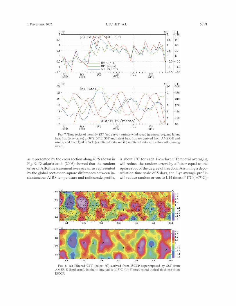
Figure 6b shows that evaporative cooling is enhancedover areas of collocated warmer water and higher ENWand reduced over areas of lower SST and lower ENW.Typical time series were shown in Fig. 7a as an ex-ample, illustrating the positive contemporary correla-tion among the three parameters after filtering. HigherSST causes higher wind and evaporation almost instan-taneously. The filtering, in effect, removes the low-frequency variation (annual cycle). Without filtering,however, the annual cycle dominates (Fig. 7b). Evapo-

ration is opposite in phase with the temporal rate ofchange of SST, which is in quadrature with SST itself.Higher wind speed and higher evaporation during win-ter start the cooling, which results in the lowest SSToccurring a few months later. The contemporary corre-lation between wind speed and SST will be negative, asdescribed in previous studies over global ocean (e.g.,Liu et al. 1994). More explanations and implications aregiven in section 4c.

f. Upper atmosphere signatures

Figure 8a shows that, averaged over the same 5-yrperiod, the ISCCP CTT anomalies have a similar dis-tribution as SST anomalies. Clear-sky pixels were re-moved in this dataset to eliminate the influence by sur-face temperature. Figure 8b shows that optically thickerclouds are observed to be collocated with higher CTTand SST and vice versa. Cloud-top pressure fromISCCP data varies from 570 mb over the cold eddies(e.g., 26°E) to 650 mb over the warm eddies (e.g.,30°E), but the values are derived from the temperaturefield based on knowledge of the atmospheric tempera-ture profile and are not directly observed from space-based sensors. Nonetheless, it implies that the cloud topis high above the usual height of atmospheric boundarylayer (900 mb). The collocation of CTT and SSTanomalies indicates interaction between SST and theatmosphere way above the atmospheric boundarylayer.

AIRS temperature soundings show that the high- andlow-temperature anomalies, collocated with warm andcold ocean eddies, penetrate all the way up to 300 mb,

FIG. 6. (a) Filtered surface ENW convergence (color, 10�5 s�1) and (b) latent heat flux(color, W m�2), both superimposed by SST (isotherms). Isotherm interval is 0.15°C. TheENW convergence is derived from QuikSCAT, and latent heat flux is derived from AMSR-E.


Fig 6 live 4/C

as represented by the cross section along 40°S shown inFig. 9. Divakarla et al. (2006) showed that the randomerror of AIRS measurement over ocean, as representedby the global root-mean-square differences between in-stantaneous AIRS temperature and radiosonde profile,

is about 1°C for each 1-km layer. Temporal averagingwill reduce the random errors by a factor equal to thesquare root of the degree of freedom. Assuming a deco-rrelation time scale of 5 days, the 3-yr average profilewill reduce random errors to 1/14 times of 1°C (0.07°C).

FIG. 8. (a) Filtered CTT (color, °C) derived from ISCCP superimposed by SST fromAMSR-E (isotherms). Isotherm interval is 0.15°C. (b) Filtered cloud optical thickness fromISCCP.

FIG. 7. Time series of monthly SST (red curve), surface wind speed (green curve), and latentheat flux (blue curve) at 39°S, 35°E. SST and latent heat flux are derived from AMSR-E andwind speed from QuikSCAT. (a) Filtered data and (b) unfiltered data with a 3-month runningmean.



Even with a 10-day decorrelation time scale, the accu-racy will still be better than 0.1°C. The 0.1°–0.2°Canomalies shown in Fig. 9 are significant. Tian et al.(2006) demonstrated that AIRS temperature anomaliesof similar magnitude could be successfully used to studyMadden–Julian oscillation.

The correlation coefficients of the geographic varia-tions (585 pairs of data at a 0.5° grid in the region of42°–38°S, 23°–55°E) between SST and CTT for 3-yr,1-yr, and 3-month periods are nearly constant, over 0.7;they decrease to around 0.65, 0.5, and 0.4 at 1-month,10-day, and 5-day periods, respectively. The correlationcoefficients between SST and upper-level AIRS tem-perature (e.g., 600 mb) also decrease with shorter av-eraging periods, but with sharper drops at short peri-ods, from over 0.6 at 1 yr to 0.15 at 5 days.

If one assumes 585/4 (every other grid point) as thedegree of freedom, a correlation coefficient of 0.16 willmeet the 95% confidence criterion. If we use 585/9 (ev-ery third grid point) as the degree of freedom, a corre-lation coefficient of 0.24 will meet the 95% confidentlevel. An additional significance test is performed usingMonte Carlo simulation. The 585 pairs of data wereselected randomly from all 10-day and monthly aver-ages separately, and the correlation coefficients werecomputed repeatedly 1000 times to obtain a normaldistribution. In both cases, the 95% confidence level is0.085. Except for the time period of 5 days and shorter(synoptic time scales) the spatial correlations are sig-nificant.

4. Discussions

a. Ocean dynamics

The AMSR-E SST and SeaWiFS chlorophyll clearlysupport the identification of the AEC semipermanentmeanders by Lagrangian drifters. The locations of theanomalies are in agreement with the short-duration

cruise measurements during the Cape of Good HopeExperiments (KAPEX; Boebel et al. 2003), which arelargely made in the western region. When comparedwith drifter measurements averaged for the previous 5yr (January 1995 to December 1999), the locations ofthe eddies west of 35°E remain unchanged, while thelocations of the eastern eddies are less well defined.The agreement at different time periods demonstratesthe quasi-steady nature of the meandering jets, firstidentified by Pazan and Niiler (2004) using drifter mea-surements from 1978 to 2003.

The dynamic balance of similar quasi-steady frontshas been postulated by Niiler et al. (2003), Hughes(2005), and Ochoa and Niiler (2007). While the zonalorientation of chlorophyll concentration in the Circum-polar Current observed by SeaWiFS has been investi-gated (e.g., Moore and Abbott 2000; Pollard et al.2002), the strong chlorophyll concentration poleward ofthe maximum AEC current, as shown in Fig. 2, has notbeen discussed and the mechanism of its formation,whether it is due to horizontal transport or upwelling, isunknown.

b. Feedback on current

As explained in section 2a, � depends on wind shear,or the difference between the wind vector near the sur-face and the surface current. The importance of surfacecurrent feedback on the determination of stress in thetropical ocean was studied by simulation using oceangeneral circulation models (e.g., Pacanowski 1987).While surface current has been included in some of theformulation of bulk parameterization of stress (e.g., Liuet al. 1979), it is generally assumed to be negligiblecompared with wind. Scatterometer data show thatsuch assumption is not valid when the magnitude ofwind relative to current is low, as over tropical oceans(Kelly et al. 2001), and when there is directional differ-ence caused by current rotation. Because ocean surface

FIG. 9. Vertical structure of filtered air temperature (°C) across 40°S from AIRS data.Circles and stars are projected locations of the SST anomaly centers shown in Fig. 2b.


Fig 9 live 4/C

current is not used as boundary conditions, NWPdata could not produce the rotation � with the currenteffect.

The rotation of ENW in opposition to the rotation ofthe surface current observed over the AEC is in agree-ment with the observation of Cornillon and Park (2001)over the Gulf Stream rings. It clearly demonstrates thatthe scatterometer measures stress rather than winds.The opposite sign of the vorticity also implies that thestress anomalies spin down the current rotation throughmomentum transport. The small magnitude of ENWvorticity anomalies compared with those of the oceancurrent anomalies implies that ocean current dominatesin the long-term mesoscale vorticity coupling.

The ENW vorticity anomalies (Fig. 4b) are collo-cated (and opposite in phase) with ocean current andSST anomalies; they should be in quadrature with thevorticity caused by the crosswind SST gradient de-scribed in the introduction. O’Neill et al. (2005), usinga broader filter, show the in-phase correlation betweenENW vorticity and crosswind SST gradient over alarger region that includes the entire Agulhas Currentsystem and circumpolar currents. However, over thesmaller region we examined (38°–41°S, 25°–37°E), bothO’Neill’s and our results show that the correlation be-tween ENW vorticity and crosswind SST gradient isweak and the effect of surface current vorticity onENW vorticity dominates.

c. Feedback on ocean temperature

The latent heat flux, as represented by conventionalbulk parameterization, is

LH � �aCeLu�Q�Ts� � rQ�Ts � �T� ,

where L is the latent heat of vaporization, �a is surfaceair density, Ce is the water vapor transfer coefficient, ris the relative humidity, Ts is SST, �T is sea–air tem-perature difference, and Q(T) is the saturation specifichumidity at temperature T. Atmospheric turbulentmixing is fast. The temporal variation of LH, u, and Ts

are in phase. The contemporary positive correlationsamong the filtered SST, u, and LH over the mesoscaleeddies are the result of the ocean driving the atmo-sphere.

A simplified representation of the heat balance in awell-mixed layer of the upper ocean of depth h withtemperature approximately equal to Ts is

�wch�Ts

�t� A � LH,

where �w is the surface water density, c is isobaric spe-cific heat of water, and A is the sum of ocean heatadvection (horizontal and vertical), the surface radia-tive flux, and sensible heat flux into the layer. The timeseries in Fig. 7b shows the atmosphere driving theocean. While the variation of LH is opposite in phasewith Ts/t, it is in quadrature with Ts (sine and cosinefunctions). If the temporal variation is dominated bythe annual cycle, Ts may lag LH by a season. It takestime for LH to cool the ocean surface layer. Figure 7bshows that the low SST lags the high wind and highlatent heat flux, and this negative correlation betweenwind speed and SST is prevalent if the low-frequencyvariation is retained. The results are consistent with theanalysis of large-scale and low-frequency variationsover the global ocean using space-based data by Liu etal. (1994). Another major factor is the solar heating; itsannual variation is shown by Liu et al. (1994) to be inphase with Ts/t. How the mesoscale variation ofevaporation affects low-frequency variation or atmo-spheric buoyancy and convection remains to be ascer-tained.

d. Feedback on stress

The spatial coherence of SST with ENW both mea-sured by QuikSCAT and computed in our conceptualexperiment of horizontally homogeneous wind speed,supports that QuikSCAT measures stress rather thanwind. If the spatial coherence between scatterometerobservations and SST is mainly caused by the depen-dence of turbulent mixing with atmospheric densitystratification, as postulated by almost all the past stud-ies (cited in the introduction), the coherence should beinherent in the definition of ENW. Any discrepancies,if realistic, may suggest the present scatterometermodel function does not accurately retrieve ENW orthe need of additional positive feedback to the turbu-lent mixing mechanism.

Unfortunately, high-resolution atmospheric tem-perature and humidity measurements are not availableto derive the stability parameters and ascertain the dis-crepancies in the conceptual experiment; NCEP tem-perature and humidity may not sufficiently representthe long-term, high-resolution features over AEC. Thewinds should not be spatially uniform, but constantlyadjusting to the ocean fronts, through turbulent trans-port and response to large-scale thermodynamics. Thecomputed ENW, of course, depends on the stabilityfunction , which represents the state-of-art knowledgeof turbulence parameterization. Although there havebeen many investigations to improve the drag coeffi-cient (e.g., Fairall et al. 1996) in past few decades, thereis no significant change in the formulation of .


There are various error sources for ENW related toSST. The model function might be calibrated notagainst ENW but the actual winds. Except for the pre-flight model function for the NASA Scatterometer(NSCAT) [called Seasat-A Satellite Scatterometer(SASS-2)], which was adjusted with ENW computedfrom in situ measurements (e.g., JASIN experiment)collected for Seasat validation, most tuning of revisedmodel functions (e.g., NSCAT-1, NSCAT-2) was basedon NWP wind products (e.g., Wentz and Smith 1999)that are not ENW. ENW errors depend on the historyof calibration and are difficult to gauge. Surface stress(or ENW) depends on surface viscosity, which varieswith SST. A small secondary effect of stress depen-dence on viscosity at weak winds was observed by Liu(1984), in agreement with postulation of Lleonart andBlackman (1980). According to the postulation, thebackscatter coefficient and ENW would be higher athigher viscosity and lower SST, in opposite to the ob-served relation between ENW and SST presented insection 3c.

Turbulent mixing may not be able to account for allthe ENW or stress anomalies related to SST. Convec-tive mixing may be the additional mechanism to en-hance the horizontal stress anomalies across the tem-perature front. QuikSCAT observations show that thevariation of ENW divergence anomalies are in quadra-ture with SST similar to the results of Xie et al. (1998)and Liu et al. (2000), in the tropical Pacific, or in phasewith downwind temperature gradient as described byChelton et al. (2001). As illustrated in Fig. 6a, conver-gence found on the downwind side of local SST maximamay result in ascending air and divergence on the up-wind side may result in descending air, reversed diver-gence and vertical motions on the two sides of SSTminima. The result of the convective cell may be a posi-tive feedback to the ENW–SST coherence resultingfrom stability difference; it accelerates ENW overwarm water and decelerates ENW over cool water. Thequestion is how high does such convection go over along period of time.

e. Possible effect on upper troposphere

Past studies of atmospheric responses to ocean ther-mal fronts, whether through observations or numericalexperiments, explored only the limited effects on theatmospheric boundary layer. Strong synoptic variabilityand atmospheric forcing are believed to be more im-portant than ocean forcing in the midlatitudes. TheAIRS soundings and ISCCP data show that the thermaleffect extends far above the boundary layer. It is ap-parent that the whole atmosphere warms and forms

optically thicker clouds over warmer water and coolsand forms optically thinner clouds over cooler water.Accurate measurement of vertical velocity is not avail-able to examine the dynamics. The dynamics and ther-modynamics of such behavior need to be addressed infuture study. There is likely to be significant cloud–SSTfeedback (Ramanathan and Collins 1991; Fu et al. 1996;Lin et al. 2002) that also requires further investigation.The high-resolution ECMWF and NCEP vertical tem-perature profiles do not show the penetrating tempera-ture effects as in the AIRS soundings. It is questionablewhether the operational atmospheric models have suf-ficient mesoscale thermodynamics to produce realisticlong-term means.

5. Conclusions

The recent push from research to operational appli-cations of a space-based scatterometer has channeledmuch community effort in articulating scatterometer asa wind-measuring instrument for operational numericalweather and tropical cyclone predictions. The originaljustification for the scatterometer, however, came fromoceanographers who need surface wind forcing of theocean (O’Brien 1982). Ocean surface stress, rather thanwind, is the momentum flux, which drives ocean circu-lation that affects long-term climate changes. This studyclarifies the unique capability of the scatterometer inmeasuring stress over global ocean, night and day, clearand cloudy, at high spatial resolution. The dependenceof scatterometer measurements on ocean surface cur-rent and SST should not be viewed as wind error orwind anomalies but as the natural characteristics of sur-face stress. For a long time, stress has been derived onlyfrom wind, and its dependence on ocean variability hasmostly been neglected. Scatterometer measurementsare casting new light on stress and will improve futureresearch and operational, meteorological, and oceanicapplications.

There has been continuous improvement in the spa-tial resolution of NWP outputs. The use of high-resolution SST as boundary condition (starting May2001 at ECMWF) and the assimilation of QuikSCATdata (starting in January 2002 for both NCEP andECMWF) should have improved the operational sur-face wind products. But without inputs of ocean param-eters, such as surface currents, surface waves, and seastate, improving stress estimation would be difficult.Our present parameterization of stress in terms of windis not sufficient over ocean fronts, and perhaps, in se-vere storms. Direct measurements of stress from space-borne scatterometers, without the need of deriving itfrom the wind vector, are critically needed.


The Agulhas Currents continuously supply energy tomaintain the current shears and surface temperaturegradients that cause the instability in the atmosphereand generate turbulent mixing. Atmospheric turbu-lence tends to dissipate the energy, reduces the insta-bility, and provides a negative feedback to smooth outthe ocean gradients. In the atmosphere, the effect ofocean fronts may include positive feedback on convec-tive mixing that enhances the horizontal stress gradient.Dynamic linkage of surface turbulent transfer to large-scale circulation and cloud–radiative feedback, in thefuture, will require multi-year and high-resolution datawith sufficient coverage from a combination of space-based sensors.

Experimental investigation of air–sea interactionnear ocean fronts has been mostly on synoptic timescales and within the boundary layer; the validations ofspace-based observations are mostly made at synoptictime scales. The results of this study show potentialeffects of surface anomalies near the ocean front, inlong periods and high into the atmosphere; the effectsare important to climate changes and radiation balancein the atmosphere. Present NWP models may not havethe physics to simulate the long-term, penetrating ef-fects, making space-based observations (e.g., ISCCPand AIRS) all the more important in the characteriza-tion, understanding, and prediction of climate changes.This study demonstrates the synergism of five sets ofspace-based measurements, QuikSCAT, AMSR-E,SeaWiFS, AIRS, and ISCCP and the surface currentmeasured by the Lagrangian drifters.

Acknowledgments. This study was conducted at theJet Propulsion Laboratory, California Institute of Tech-nology, under contract of NASA. It was jointly sup-ported by the Physical Oceanography, Ocean VectorWind, Earth Observing System, and the Energy andWater Cycle Programs of NASA. William Rossow, EricFetzer, Hartmut Aumann, and Moustafa Chahinekindly reviewed and advised on the analyses of ISCCPand AIRS data.

REFERENCES

Boebel, O., T. Rossby, J. Lutjeharms, W. Zenk, and C. Barron,2003: Path and variability of the Agulhas Return Current.Deep-Sea Res. II, 50, 35–56.

Brown, R. A., and W. T. Liu, 1982: An operational large-scalemarine planetary boundary layer model. J. Appl. Meteor., 21,261–269.

Chahine, M. T., and Coauthors, 2006: AIRS: Improving weatherforecasting and providing new data on greenhouse gases.Bull. Amer. Meteor. Soc., 87, 911–926.

Chelton, D. B., and Coauthors, 2001: Observations of couplingbetween surface wind stress and sea surface temperature inthe eastern tropical Pacific. J. Climate, 14, 1479–1498.

——, M. G. Schlax, M. H. Freilich, and R. Milliff, 2004: Satellitemeasurements reveal persistent small-scale features in oceanwinds. Science, 303, 978–983.

Cornillon, P., and K.-A. Park, 2001: Warm core ring velocitiesinferred from NSCAT. Geophys. Res. Lett., 28, 575–578.

Cronin, M. F., S.-P. Xie, and H. Hashizume, 2003: Barometricpressure variations associated with eastern Pacific tropicalinstability waves. J. Climate, 16, 3050–3057.

Divakarla, M. G., C. D. Barnet, M. D. Goldberg, L. M. McMillin,E. Maddy, W. Wolf, L. Zhou, and X. Liu, 2006: Validationof Atmospheric Infrared Sounder temperature and water va-por retrievals with matched radiosonde measurementsand forecasts. J. Geophys. Res., 111, D09S15, doi:10.1029/2005JD006116.

Fairall, C. W., E. F. Bradley, D. P. Rogers, J. B. Edson, and G. S.Young, 1996: Bulk parameterization of air-sea fluxes forTropical Ocean-Global Atmosphere Coupled Ocean-Atmosphere Response Experiment. J. Geophys. Res., 101,3747–3764.

Fleagle, R. G., and J. A. Businger, 1963: An Introduction to At-mospheric Physics. Academic Press, 346 pp.

Friehe, C. A., and Coauthors, 1991: Air-sea fluxes and surfacelayer turbulence around a sea surface temperature front. J.Geophys. Res., 96 (C5), 8593–8609.

Fu, R., W. T. Liu, and R. E. Dickinson, 1996: Response of tropicalclouds to the interannual variation of sea surface tempera-ture. J. Climate, 9, 616–634.

Geernaert, G., 1990: Bulk parameterizations for the wind stressand heat fluxes. Current Theory, G. Geernaert and W. J.Plant, Eds., Vol. 1, Surface Waves and Fluxes, Kluwer Aca-demic, 91–172.

Greenhut, G. K., 1982: Stability dependence of fluxes and bulktransfer coefficients in a tropical boundary layer. Bound.-Layer Meteor., 24, 253–264.

Guymer, T. H., J. A. Businger, K. B. Katsaros, W. J. Shaw, P. K.Taylor, W. G. Large, and R. E. Payne, 1983: Transfer pro-cesses at the air–sea interface. Philos. Trans. Roy. Soc. Lon-don, A308, 253–273.

Hashizume, H., S.-P. Xie, M. Fujiwara, M. Shiotani, T. Watanabe,Y. Tanimoto, W. T. Liu, and K. Takeuchi, 2002: Direct ob-servations of atmospheric boundary layer response to SSTvariations associated with tropical instability waves over theeastern equatorial Pacific. J. Climate, 15, 3379–3393.

Hayes, S. P., M. J. McPhaden, and J. M. Wallace, 1989: The influ-ence of sea-surface temperature on surface wind in the east-ern equatorial Pacific: Weekly to monthly variability. J. Cli-mate, 2, 1500–1506.

Hughes, C. W., 2005: Nonlinear vorticity balance of the AntarcticCircumpolar Current. J. Geophys. Res., 110, C11008,doi:10.1029/2004JC002753.

Kelly, K. A., S. Dickinson, M. J. McPhaden, and G. C. Johnson,2001: Ocean currents evident in satellite wind data. Geophys.Res. Lett., 28, 2469–2472.

Kushnir, Y., W. A. Robinson, I. Bladé, N. M. J. Hall, S. Peng, andR. Sutton, 2002: Atmospheric GCM response to extratropicalSST anomalies: Synthesis and evaluation. J. Climate, 15,2233–2256.

Lau, N.-C., and M. J. Nath, 1994: A modeling study of the relativeroles of tropical and extratropical SST anomalies in the vari-ability of the global atmosphere–ocean system. J. Climate, 7,1184–1207.

Lin, B., B. Wielicki, L. Chambers, Y. Hu, and K.-M. Xu, 2002: The


iris hypothesis: A negative or positive cloud feedback? J.Climate, 15, 3–7.

Lin, I.-I., W. T. Liu, C.-C. Wu, J. C. H. Chiang, and C.-H. Sui,2003: Satellite observations of modulation of surface windsby typhoon-induced upper ocean cooling. Geophys. Res.Lett., 30, 1131, doi:10.1029/2002GL015674.

Liu, W. T., 1984: The effects of the variations in sea surface tem-perature and atmospheric stability in the estimation of aver-age wind speed by SEASAT-SASS. J. Phys. Oceanogr., 14,392–401.

——, 2002: Progress in scatterometer application. J. Oceanogr.,58, 121–136.

——, and W. G. Large, 1981: Determination of surface stress bySeasat-SASS: A case study with JASIN data. J. Phys. Ocean-ogr., 11, 1603–1611.

——, and W. Tang, 1996: Equivalent neutral wind. JPL Publica-tion 96-17, Jet Propulsion Laboratory, California Institute ofTechnology, Pasadena, CA, 16 pp.

——, and X. Xie, 2002: Double intertropical convergencezones—A new look using scatterometer. Geophys. Res. Lett.,29, 2072, doi:10.1029/2002GL015431.

——, and ——, 2006: Measuring ocean surface wind from space.Remote Sensing of Human Settlements, M. K. Ridd and J. D.Hipple, Eds., Manual of Remote Sensing, Vol. 5, AmericanSociety for Photogrammetry and Remote Sensing, 149–178.

——, K. B. Katsaros, and J. A. Businger, 1979: Bulk parameter-ization of air-sea exchanges of heat and water vapor includingthe molecular constraints at the interface. J. Atmos. Sci., 36,1722–1735.

——, W. Tang, and P. P. Niiler, 1991: Humidity profiles over theocean. J. Climate, 4, 1023–1034.

——, A. Zhang, and J. Bishop, 1994: Evaporation and solar irra-diance as regulators of sea surface temperature in annual andinterannual changes. J. Geophys. Res., 99, 12 623–12 638.

——, W. Tang, and R. Atlas, 1996: Responses of the tropicalPacific to wind forcing as observed by spaceborne sensorsand simulated by an ocean general circulation model. J. Geo-phys. Res., 101, 16 345–16 360.

——, X. Xie, P. S. Polito, S.-P. Xie, and H. Hashizume, 2000:Atmospheric manifestation of tropical instability wave ob-served by QuikSCAT and Tropical Rain Measuring Mission.Geophys. Res. Lett., 27, 2545–2548.

Liu, Z., and L. Wu, 2004: Atmospheric response to North PacificSST: The role of ocean–atmosphere coupling. J. Climate, 17,1859–1882.

Lleonart, G. T., and D. R. Blackman, 1980: The spectral charac-teristics of wind-generated capillary waves. J. Fluid Mech., 97,455–479.

Luis, A. J., and P. C. Pandey, 2005: Characteristics of atmosphericdivergence and convergence in the Indian Ocean inferredfrom scatterometer winds. Remote Sens. Environ., 97, 231–237.

McClain, C. R., G. C. Feldman, and S. B. Hooker, 2004: An over-view of the SeaWiFS project and strategies for producing aclimate research quality global ocean bio-optical time series.Deep-Sea Res. II, 51, 5–42.

Moore, J. K., and M. R. Abbott, 2000: Phytoplankton chlorophylldistributions and primary production in the Southern Ocean.J. Geophys. Res., 105, 28 709–28 722.

Niiler, P. P., 2001: The World Ocean surface circulation. OceanCirculation and Climate: Observing and Modelling the GlobalOcean, G. Siedler, J. Church, and J. Gould, Eds., Interna-tional Geophysics Series, Vol. 77, Academic Press, 193–204.

——, N. A. Maximenko, and J. C. McWilliams, 2003: Dynamicallybalanced absolute sea level of the global ocean derived fromnear-surface velocity observations. Geophys. Res. Lett., 30,2164, doi:10.1029/2003GL018628.

Nonaka, M., and S.-P. Xie, 2003: Covariations of sea surface tem-perature and wind over the Kuroshio and its extension: Evi-dence for ocean-to-atmosphere feedback. J. Climate, 16,1404–1413.

O’Brien, J. J., 1982: Scientific Opportunities Using Satellite SurfaceStress Measurements Over the Ocean–Report of the SatelliteSurface Stress Working Group. Nova University Press,163 pp.

Ochoa, J., and P. P. Niiler, 2007: Vertical vorticity balance in me-anders downstream the Agulhas retroflection. J. Phys.Oceanogr., 37, 1740–1744.

O’Neill, L. W., D. B. Chelton, and S. Esbensen, 2003: Observa-tions of SST-induced perturbations of the wind stress fieldover the Southern Ocean on seasonal time scales. J. Climate,16, 2340–2354.

——, ——, ——, and F. J. Wentz, 2005: High-resolution satellitemeasurements of the atmospheric boundary layer response toSST variations along the Agulhas Return Current. J. Climate,18, 2706–2723.

Pacanowski, R. C., 1987: Effect of equatorial currents on surfacestress. J. Phys. Oceanogr., 17, 833–838.

Park, K.-A., and P. Cornillon, 2002: Stability-induced modifica-tion of sea surface winds over Gulf Stream rings. Geophys.Res. Lett., 29, 2211, doi:10.1029/2001GL014236.

Pazan, S. E., and P. P. Niiler, 2004: Ocean sciences: New globaldrifter data set available. Eos, Trans. Amer. Geophys. Union,85, 17.

Polito, P. S., J. P. Ryan, W. T. Liu, and F. P. Chavez, 2001: Oce-anic and atmospheric anomalies of tropical instability waves.Geophys. Res. Lett., 28, 2233–2236.

Pollard, R. T., M. I. Lucas, and J. F. Read, 2002: Physical controlson biogeochemical zonation in the Southern Ocean. Deep-Sea Res. II, 49, 3289–3305.

Ramanathan, V., and W. Collins, 1991: Thermodynamic regula-tion of ocean warming by cirrus clouds deduced from obser-vations of the 1987 El Niño. Nature, 351, 27–32.

Rossow, W. B., and R. A. Schiffer, 1999: Advances in understand-ing clouds from ISCCP. Bull. Amer. Meteor. Soc., 80, 2261–2287.

Small, R. J., S.-P. Xie, and Y. Wang, 2003: Numerical simulationof atmospheric response to Pacific tropical instability waves.J. Climate, 16, 3723–3741.

Song, Q., T. Hara, P. Cornillon, and C. A. Friehe, 2004: A com-parison between observations and MM5 simulations of themarine atmospheric boundary layer across a temperaturefront. J. Atmos. Oceanic Technol., 21, 170–178.

Tennekes, H., and J. L. Lumley, 1972: A First Course in Turbu-lence. MIT Press, 300 pp.

Tian, B., D. E. Waliser, E. J. Fetzer, B. H. Lambrigtsen, Y. L.Yung, and B. Wang, 2006: Vertical moist thermodynamicstructure and spatial–temporal evolution of the MJO inAIRS observations. J. Atmos. Sci., 63, 2462–2485.

Vecchi, G. A., S.-P. Xie, and A. S. Fischer, 2004: Ocean–atmosphere covariability in the western Arabian Sea. J. Cli-mate, 17, 1213–1224.

Wentz, F. J., and D. K. Smith, 1999: A model function for theocean-normalized radar cross section at 14 GHz derived fromNSCAT observations. J. Geophys. Res., 104, 11 499–11 514.


——, and T. Meissner, 2000: Algorithm Theoretical Basis Docu-ment (ATBD) version 2: AMSR ocean algorithm. RemoteSensing Systems Tech. Rep. 121599A, 59 pp.

——, C. L. Gentemann, D. Smith, and D. Chelton, 2000: Satellitemeasurements of sea surface temperature through clouds.Science, 288, 847–850.

White, W. B., and J. L. Annis, 2003: Coupling of extratropicalmesoscale eddies in the ocean to westerly winds in the atmo-spheric boundary layer. J. Phys. Oceanogr., 33, 1095–1107.

Xie, S.-P., 2004: Satellite observations of cool ocean–atmosphereinteraction. Bull. Amer. Meteor. Soc., 85, 195–208.

——, M. Ishiwatari, H. Hashizume, and K. Takeuchi, 1998:Coupled ocean-atmospheric waves on the equatorial front.Geophys. Res. Lett., 25, 3863–3866.

——, J. Hafner, Y. Tanimoto, W. T. Liu, H. Tokinaga, and H. Xu,2002: Bathymetric effect on the winter sea surface tempera-ture and climate of the Yellow and East China Seas. Geo-phys. Res. Lett., 29, 2228, doi:10.1029/2002GL015884.

Yu, J.-Y., and W. T. Liu, 2003: A linear relationship betweenENSO intensity and tropical instability wave activity in theeastern Pacific Ocean. Geophys. Res. Lett., 30, 1735,doi:10.1029/2003GL017176.


ocean–atmosphere interaction over agulhas extension … · ocean–atmosphere interaction over...

Documents