c O s Pa r 2010

Earth sciEncEs

84

Oceanography

Operational space oceanography has startedThanks to its historical strong involvement and expertise in space oceanography, CNES has been exercising a wide variety of activities and partnerships in that field. It has been involved in all aspects of it, from research to deve-lopment and operation. Its subsidiaries CLS and Mercator Océan are testimonies of this.

With the Jason program, space altimetry becomes operationalJune 20, 2008 will surely be remembered in the history of oceanography as the day space oceanography truly became operational. On that day, Jason-2 was launched success-fully from the Californian Air Force Base of Vandenberg. The result of a cooperation between CNES, NASA, Eumet-sat and NOAA, this mission is the successor of Jason-1. The two satellites were placed during a few months in a close formation, less than a minute from each other in order to calibrate the two systems with one another with millimetric precision. Then, in February 2009, Jason-1 was moved to a more complementary orbit in order to optimize the space and time coverage of the two satellites for the benefit of the oceanographic community.

Jason-2, an improvement of Jason-1While walking in the footsteps of Jason-1, Jason-2 has been equipped with the latest technologies in the field of space

altimetry. Its new capabilities will enable it to follow the level of coastal waters, lakes, and the biggest rivers with a never-before-achieved precision.Its oceanographic performance has already exceeded that of Jason-1 in part thanks to a precise measuring system which combines the best available technologies to date: DORIS, GPS and laser reflectometry. Jason-1 and Jason-2 are the refer-ence missions enabling to establish the long-term evolution maps of sea level, a precious indicator for the Intergovern-mental Panel on Climate Change (IPCC). The Jason products are now distributed by Eumetsat and NOAA to the various operational users, and by CNES and NASA to more than a thousand research teams around the globe. Building on this success, Eumetsat and NOAA have decided to lead the Jason-3 mission, whose launch is expected in 2013. In late 2009, CNES gave its approval to act as contracting owner, and the program started in February 2010, as soon as Eumetsat obtained the decision from its member states.

AltiKa before Sentinel-3Around 2013, the GMES Sentinel-3A mission will complete the Jason-2 and Jason-3 missions, thanks to its helio- synchronous orbit. Meanwhile, in order to minimize the risk of zero service for end users, CNES, in cooperation with ISRO, the Indian space agency, launched the development of the satellite SARAL (Satellite with ARgos and ALtiKa). This satellite will be placed on ENVISAT’s orbit in 2011, and its Ka band altimeter will provide the necessary entry data for assimilation models and scientific teams.

AUTHORE. Thouvenot

[Fig. 1] [Fig. 2]

85

(Surface Wave Investigation and Monitoring). China will also provide, apart from the platform and the launch, a complementary instrument to SWIM called SCAT, whose aim is to measure the wind fields on the surface of the waves. The program is entering development phase, and launch is expected in 2014. The mission will be part of a broad cooperation between France and China in the field of space oceanography. As early as 2011, the Chinese HY-2A altimetry satellite will carry a DORIS precise orbit measuring instrument.

The CNES seminar of scientific prospective held in 2009 also enabled to define the research priorities for the next decade. The main themes which already undergo feasibility studies at CNES are wide-swath altimetry and ocean colour measur-ing in geostationary orbit to define biological parameters.

Oceanography

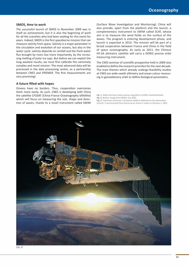
Fig. 1: AltiKa electronic boxes during integration of SARAL Payload Module.Fig. 2: Redsea, image from MODIS, July 2003.Fig. 3: Impression of Envisat, a European platform dedicated to the observation of Earth. It was launched from Kourou by an Ariane 5 rocket on February 2, 2002.

SMOS, time to workThe successful launch of SMOS in November 2009 was in itself an achievement, but it is also the beginning of work for all the scientists who had been waiting for this event for years. Indeed, SMOS is the first spaceborne mission that can measure salinity from space. Salinity is a major parameter in the circulation and evolution of our oceans, but also in the water cycle: salinity depends on rainfall and the fresh water flux brought by rivers but more importantly, by the increa-sing melting of polar ice caps. But before we can exploit the long awaited results, we must first calibrate this extremely complex and novel mission. The most advanced data will be processed in the data processing centre, as a partnership between CNES and IFREMER. The first measurements are very promising!

A future filled with hopesOceans have no borders. Thus, cooperation overcomes them more easily. As such, CNES is developing with China the satellite CFOSAT (China-France Oceanography SATellite) which will focus on measuring the size, shape and direc-tion of waves, thanks to a novel instrument called SWIM

[Fig. 3]

c O s Pa r 2010

86

Laboratory contr ibut ionEarth sciEncEs

Abstract

With an observational period of more than 20 years of satellite chlorophyll and sea surface temperature, researchers from the Laboratoire d’océanographie de Villefranche have highlighted that the distribution and abundance of phytoplankton in the Pacific and Atlantic oceans depend on these basins’ decadal physical oscillations. They demonstrate the need to take into account such fluctuations into models to improve forecasts of phytoplankton evolution in response to global environmental changes.

Avec plus de 20 ans d’observations par satellite de la chlorophylle et des température de surface, des chercheurs du LOV ont montré que la distribution et l’abondance en phytoplancton dans le Pacifique et l’Atlantique dépendent des oscillations décennales des propriétés physiques de ces bassins. Ces oscillations doivent être prises en compte dans les modèles pour améliorer les prévisions de réponse du phytoplancton face aux changements environnementaux globaux.

Influence of decadal climate oscillations of ocean basins on phytoplankton.

Influence des oscillations climatiques décennales des bassins océaniques sur le phytoplancton.

Laboratoire d’océanographie de Villefranche (LOV), quai de la Darse, BP 8, 06238 Villefranche-sur-Mer Cedex, France.

Phytoplankton are unicellular algae that in-habit the upper layer of the ocean (from a few tens of meters to ~200 m). They need CO2 to grow, thus affecting the ocean and atmosphere CO2 levels and playing an essential role in the global carbon cycle. Therefore it is important to estimate the concentration of phytoplankton at global scale and to under-stand how their distribution and abundance are affected by ocean variability. Physical processes, e.g. ocean circulation, heat balance, atmospheric conditions at the ocean surface etc., occur on a variety of time scales: interdecadal at basin or global scales, interannual and seasonal, and probably the cen-tennial one associated with anthropogenic global warming.

The best way to assess phytoplankton concentrations at global scale is to estimate chlorophyll concentration (Chl) using radiometers on board Earth observation satellites. This technique was initiated around 30 years ago. It is referred to as “ocean color” or “Visible Spectral Radiometry” (VSR), and has resulted in long time series of Chl at global scale. However, understanding phytoplankton changes induced by decadal cycles in the oceans remains difficult.

LOV researchers were interested in two time series of ocean color, provided twenty years apart by the CZCS (1979-1986) and the SeaWiFS (1998-ongoing) missions. Two five-year

AUTHORSE. MartinezD. Antoine

F. D’OrtenzioB. Gentili

Oceanography

87

periods within each of these time series were reprocessed in order to homogenize them (1979-1983 and 1998-2002)[1]. A statistical analysis of these data and of Sea Surface Tempera-ture (SST) has allowed to investigate the relative variability of temporal and spatial signals of Chl and SST (Fig. 1). Pre-vious results obtained over the period 1997-2005 [2] were confirmed, namely that Chl and SST are inversely related (when one increases the other decreases and vice versa) over 75% of the ocean basins. The direction of change was however reversed between the two studies (Fig. 2). These results highlighted that Chl variability is directly related to the Pacific Decadal Oscillation (PDO) in the Pacific, and to the Atlantic Multi-decadal Oscillation (AMO) in the Atlan-tic. Observation of this SST-Chl relationship led to different interpretations depending on whether one looks at the inter-annual (2006 work) or multi-decadal scale (current work). This apparent contradiction comes from regime shifts in the oceans. The Pacific shifted from a warm to a cold regime in the 80s and then returned to a warm regime in 2002. The Atlantic shifted from a cold to a warm regime in the mid 80s. Identifying these shifts is not feasible when using time series that are too short. These results show that it is risky to interpret short-term changes (<10 years) of phyto- plankton biomass as long-term trends.

But where does this correlation between Chl and SST come from? Phytoplankton need light and nutrients to grow. However, nutrient reservoirs are in deep layers. They may be brought to the surface via the seasonal variability of the mixed layer (a) or via the variability of the nutricline depth (b). Analysis of model outputs suggests that, according to the oceanic regions and the time scales considered in the

current study, the deepening or shallowing of the nutricline is probably the mechanism behind the Chl-SST correlation.

These results provide a new framework to interpret the contemporary changes in phytoplankton. They demonstrate the importance of representing decadal oscillations in global ocean models in order to improve the predictions of the response of ecosystems to global warming. They show that the effort to build global, long-term, multi-satellite “climate data records” must be continued. Such records will provide invaluable information to understand the impact of global climate change on ocean ecosystems.(a) The ocean mixed layer is a layer where temperature and other physical properties are homogeneous, starting at the surface and extending down to a zone of strong tempera-ture gradient, called the thermocline. The thermocline is the transition between warmer surface waters and colder waters. Nutrients are brought to the surface from deep layers when the mixed layer deepens.(b) The nutricline depth is characterized by a strong gradient in nutrient concentration, above which there are few nutrients. Its depth varies in particular with the deep-ocean circulation.

Fig. 1: (Left) Chl change from the CZCS (1979-1983) to SeaWiFS (1998-2002) era, expressed as the average value ratio logarithm over the two time periods. (Right) SST (from ERSST) difference over the same period. The SST zero difference is reported on the maps as a thick black curve.Fig. 2: Mapping of areas with concomitant parallel or opposite changes of Chl and SST, as indicated. (Left) Spatial distribution observed between 1999 and 2004. (Right) as in left panel but between periods CZCS (1979-1983) and SeaWiFS (1998-2002). Data were averaged in time over each period.

References

[1] Antoine, D., Morel, A., Gordon, H.R., Banzon, V.F. and Evans, R.H. (2005), Bridging ocean color observations of the 1980’s and 2000’s in search of long-term trends, Journal of Geophysical Research, 110, C06009.

[2] Behrenfeld, M.J., Boss., E. (2006), Beam attenuation and chlorophyll concentration as alternative optical indices of phytoplankton biomass, J. Mar. Res, 64, 431-451.

[Fig. 1]

[Fig. 2]

Oceanography

c O s Pa r 2010

88

Laboratory contr ibut ionEarth sciEncEs

Abstract

Improving our knowledge of the topography of polar regions was the goal of the SPIRIT inter- national polar year project. SPIRIT allowed the acquisition of a large archive of SPOT 5 stereoscopic images covering most polar ice masses. High resolution images and Digital Elevation Models (DEMs) have been delivered freely to glaciologists in over 20 countries. This new generation of polar DEM has already been used to map changes in various regions, in particular in Southeast Alaska.

Améliorer notre connaissance de la topographie des régions polaires était l’objectif du projet Spirit durant la quatrième année polaire. Des couples d’images stéréoscopiques ont été acquis sur de nombreux glaciers polaires par le capteur Spot 5-HRS. Des images haute-résolution et des modèles numériques de terrain ont ainsi été distribués aux glaciologues. Cette nouvelle topographie des pôles est aujourd’hui utilisée pour étudier leur évolution récente, par exemple dans le Sud-Est de l’Alaska.

SPIRIT. Spaceborne mapping of polar ice masses during the fourth international polar year.

Spirit. Cartographie des glaces polaires pendant la quatrième année polaire.

1 Université de Toulouse, CNS Legos, 14 avenue Edouard Belin, 31400 Toulouse, France.2 Spot Image, 5 rue des Satellites, BP 14359, 31030 Toulouse Cedex 4, France.3 IGN Espace, 6 avenue de l’Europe, BP 42116, 31520 Ramonville Cedex, France.4 CNES, 18 avenue Edouard Belin, 31401 Toulouse Cedex 9, France.

For the last two decades, the cryosphere has experienced rapid and major changes. Shrinkage of mountain glaciers and ice caps has accelerated, with con-tribution to sea level rise growing from 0.33 mm/yr be-tween 1961 and 1990 to 0.8 mm/yr between 2001 and 2004 [1]. The break up of Larsen A and B ice shelves in the Antarctic Peninsula has led to the thinning and accel-eration of the glaciers located upstream. Major changes in the ice dynamics have also been recently detected in Greenland [2]. Thus, the cryosphere appears as one of

the major players and indicators of the ongoing climate change.

Obtaining a homogeneous and precise topography of these remote regions is important to characterize their response to recent climate change, constrain ice model-ling, quantify their contribution to sea level rise and detect future evolution. Yet, the topography of glaciers, ice caps and ice shelves remains poorly known because in situ observations are difficult and scarce. Furthermore,

AUTHORSE. Berthier 1

F. Daupras 2

M. Bernard 2

D. Lasselin 3

E. Thouvenot 4

F. Rémy 1

Oceanography

89

spaceborne measurements of the ice elevation are also challenging and not always a priority. To build a reference ice topography during the fourth International Polar Year (IPY), CNES, Spot Image, IGN Espace and LEGOS launched the SPIRIT project (SPOT 5 stereoscopic survey of Polar Ice: Reference Images and Topographies).

Fig. 1: 3D view of Barnard glacier (Alaska) derived from SPOT 5 images.Fig. 2: Map of surface elevation change in the Western Chugach Mountains between the 1950s and 2007. The thick black line corresponds to the limits of the Columbia Glacier.

Images and DEM coverage achieved during IPYThe aims of the SPIRIT project were to build a comprehen-sive archive of SPOT 5-HRS images over polar ice and, for selected regions, to produce DEMs and ortho-images that would be delivered for free to the scientific community involved in IPY projects. Over 40 scientists in 20 different countries benefited from the SPIRIT data.

The SPOT 5-HRS sensor, embedded on SPOT 5, was designed for DEM generation by acquiring stereo pairs of images along the track of the satellite. It is composed of two telescopes, pointing 20° forward and 20° backward, in relation with nadir. The short time interval between the acquisitions of the two scenes of the stereo pair (90 s) ensures very limited changes at the glacier surface and nearly identical sun illumination so that the radiometry of the two images is similar.

The target areas were the margins of the Greenland and Antarctic ice sheets and most glaciers, icefields and ice caps surrounding the Arctic Ocean and Antarctica. One major constraint was the 81.15° north – 81.15° south acquisition limit of the SPOT 5 satellite. The flat, snow-covered and homogeneous central regions of the Antarctic and Green-land ice sheets were deliberately excluded because DEMs produced by matching of optical stereo images generally contain large data gaps over homogeneous regions and would not reach the decimeter accuracy achieved using spaceborne radar or laser altimeters.

Oceanography

[Fig. 1]

[Fig. 2]

90

Earth sciEncEs Laboratory contr ibut ion

About 75% of the targeted areas were covered with cloud-free images. Cloud-free images were acquired over 1.6 × 106 km2 in the Arctic (Fig. 1) and 4.4 × 106 km2 in Antarctica. DEMs were derived over 1.3 × 106 km2 in each hemisphere. Images showing the IPY stereo images and DEM coverage are available at http://www.spotimage.com/IPY.

Using SPIRIT data to map glacier changesThe potential of SPIRIT data for glaciological studies was first demonstrated in the case of Jakobshavn Isbrae, one of the major outlet glaciers of the Greenland ice sheet. Using SPIRIT DEMs and ortho-images, the rapid thinning of the fastest glacier on Earth was mapped and found to be mostly restricted to the fast flowing part of the ice stream [3].

Recently, SPIRIT data were combined with ASTER images to provide a revised estimate of the contribution of Alaskan gla-ciers to sea level rise between 1962 and 2006 [4]. For each glacierized region of Alaska, surface elevation changes were mapped by comparing the satellite-derived DEM with the older map-derived DEM. The map of ice elevation changes for one of those regions (Western Chugach, Fig. 2) illustrates the complexity of the glacier response to climate change.

In this region, a few glaciers are thickening and advancing (in blue) but the vast majority of them are thinning (in red). In particular, the Columbia Glacier is shrinking dramati-cally: since 1980, when the retreat started, this tidewater glacier has thinned by as much as 400 m at a rate exceeding 20 m/yr. Elevation changes of Alaskan glaciers are uneven and, thus, it is difficult to sample such complex spatial varia-bility on the basis of a few field or airborne measurements. Thanks to its regional coverage, SPIRIT data make it possible to improve observations of glacial response to climate change and to specify the contribution of glaciers to sea-level rise. In total, Alaskan glaciers contributed 0.12 mm/yr to sea-level rise over the period 1962-2006.

Following these early studies in Greenland and Alaska, SPIRIT data are now being used by many glaciologists to map changes in most major glaciated polar areas such as Svalbard, Iceland, Antarctica and Greenland.

During the fourth IPY, the SPIRIT project allowed to build a unique archive of SPOT 5 high-resolution stereoscopic images. This is a precious reference dataset to study future changes of the polar cryosphere. We now hope that a similar large scale mapping campaign will be repeated within the next few years.

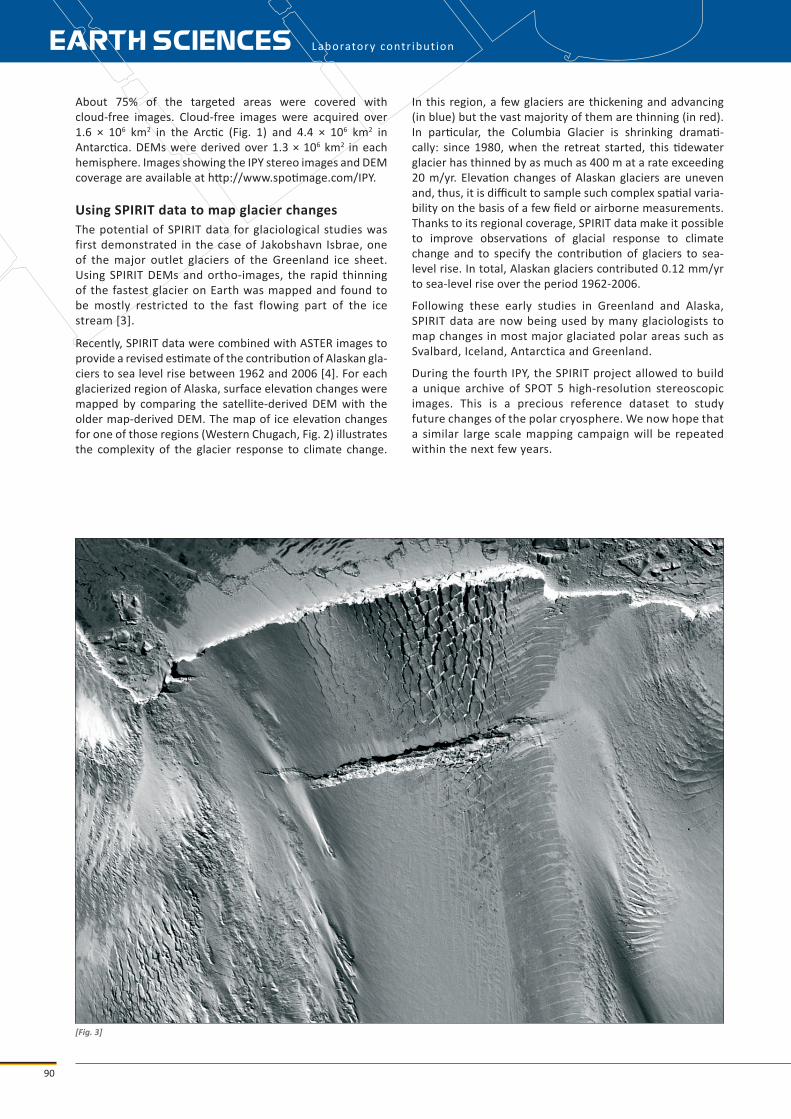
[Fig. 3]

91

References

[1] Kaser, G., et al. (2006), Mass balance of glaciers and ice caps: Consensus estimates for 1961-2004, Geophys Res Lett, 33(19), L19501.[2] Rignot, E., and P. Kanagaratnam (2006), Changes in the velocity structure of the Greenland ice sheet, Science, 311(5763), 986-990.[3] Korona, J., et al. (2009), SPIRIT. SPOT 5 stereoscopic survey of Polar Ice: Reference Images and Topographies during the fourth International Polar

Year (2007-2009), ISPRS J Photogramm, 64, 204-212.[4] Berthier, E., et al. (2010), Contribution of Alaskan glaciers to sea level rise derived from satellite imagery, Nat Geosci, 3(2), 92-95.

Fig. 3: SPOT 5 view of an outlet glacier of the Antarctic ice sheet (Dumont d’Urville area). A transverse fracture has appeared and delimits the future iceberg.Fig. 4: 3D view of the Myrdalsjökull ice cap (Iceland) derived from SPOT 5 images. Fig. 5: 3D view of Mt Erebus (Antarctica) derived from SPOT 5 images.

[Fig. 4] [Fig. 5]

Oceanography