odyssey into space aperture characterization of …...displaced-phase-center-antenna (dpca) and...

Resolution and SyntheticAperture Characterization ofSparse Radar Arrays

NATHAN A. GOODMAN, Member, IEEE

JAMES M. STILES, Senior Member, IEEEUniversity of Kansas

The concept of radar satellite constellations, or clusters, for

synthetic aperture radar (SAR), moving target indicator (MTI),

and other radar modes has been proposed and is currently

under research. These constellations form an array that is

sparsely populated and irregularly spaced; therefore, traditional

matched filtering is inadequate for dealing with the constellation’s

radiation pattern. To aid in the design, analysis, and signal

processing of radar satellite constellations and sparse arrays in

general, the characterization of the resolution and ambiguity

functions of such systems is investigated. We project the radar’s

received phase history versus five sensor parameters: time,

frequency, and three-dimensional position, into a phase history

in terms of two eigensensors that can be interpreted as the

dimensions of a two-dimensional synthetic aperture. Then, the

synthetic aperture expression is used to derive resolution and

the ambiguity function. Simulations are presented to verify the

theory.

Manuscript received December 29, 2001; revised November 19,2002 and April 7, 2003; released for publication April 7, 2003.

IEEE Log No. T-AES/39/3/818501.

Refereeing of this contribution was handled by L. M. Kaplan.

This work was supported in part by the Air Force Office ofScientific Research under Contract F49620-99-1-0172.

Authors’ current addresses: N. A. Goodman, Dept. ofElectrical and Computer Engineering, University of Arizona,1230 E. Speedway Blvd., Tucson, AZ 85721-0104, E-mail:([email protected]); J. M. Stiles, Radar Systems andRemote Sensing Laboratory, The University of Kansas, Lawrence,KS 66045.

0018-9251/03/$17.00 c 2003 IEEE

I. INTRODUCTION

As evidenced by recent literature [1–4] and by thetheme of a recent radar conference, 2001: Radar’sOdyssey into Space [5], there is currently muchinterest in moving radar technology onto spaceborneplatforms. The advantages of moving radar intospace are numerous [3, 6–7]. First, spaceborne radarsprovide global coverage, as opposed to airborne radarsthat are limited by airspace restrictions. Satellite radarsmay also reduce the amount of personnel needed tosupport surveillance operations, since no on-boardcrew is necessary. Furthermore, support personnel andthe radar asset are not as vulnerable to military threatsas they would be on an airborne platform.

One proposed concept for a space-based radar(SBR) system is to place multiple transmitters andreceivers into space, each on their own, small satellite[8–11]. These satellites, called microsats, wouldfly in a formation called a satellite constellation.Each satellite in the constellation would be able tocoherently sample the signal transmitted from each ofthe transmitters in the constellation. In this way, theconstellation would work as a single, virtual radar ableto operate in multiple modes including interferometric,synthetic aperture radar (SAR), and moving targetindicator (MTI).

The advantages of a microsat constellation arenumerous [2, 8–9, 12–14]. First, it may be lessexpensive to launch several microsats than to launch alarge satellite with the same overall antenna aperturedue partly to the possibility of using microsatsto optimize a launch vehicle’s payload capacity.Manufacturing costs are also reduced through thebenefits of mass production. In addition, a microsatconstellation degrades gracefully as individualmicrosats fail, either as expected or prematurely, andthe constellation can be reconfigured to optimizeits configuration after a failure [15]. Failure in amonolithic satellite, however, is catastrophic for theentire radar system. When microsat failure causessystem performance to fall below an acceptable level,the hardware and launch costs of a few replacementmicrosats are much less than an entire replacementsystem. Furthermore, microsat replacement canbe stretched out over time as funding becomesavailable, and system upgrades can be performedby either replacing failed microsats or augmentingconstellations with new, upgraded microsats.

The main disadvantage of a microsat constellationis that the constellation will constitute a sparselypopulated, nonuniform, three-dimensional array.Although planar, regularly spaced, tightly packedsatellite clusters have been discussed, the fuelrequirements for maintaining such a constellationare prohibitive. Consequently, radar signalprocessing algorithms previously developed forSAR and MTI are not applicable. The traditional

IEEE TRANSACTIONS ON AEROSPACE AND ELECTRONIC SYSTEMS VOL. 39, NO. 3 JULY 2003 921

displaced-phase-center-antenna (DPCA) andspace-time adaptive processing (STAP) algorithmsassume uniform, linear arrays aligned along thedirection of travel and have been applied primarilyto sidelooking scenarios. For example, the JointSurveillance Target Attack Radar System (JSTARS)uses a 24 ft phased array in along-track that ismechanically scanned in cross-track [3, 16]. Themicrosat constellation, therefore, amounts to a uniquechallenge for radar engineers. New algorithms mustbe developed to accommodate the unique arraystructure and wide range of look geometries that willbe encountered.Before effective algorithms can be developed,

however, a method for analyzing important systemcharacteristics must be established. Specifically, theconstellation’s resolution and ambiguity function mustbe determined. The importance of these parametersis obvious for SAR, but also has significance forMTI because they determine clutter rank, which is ameasure of the degrees of freedom in the collecteddata used up by ground clutter. The radar system’sresolution and ambiguity function will dependon five sensor parameters: time, frequency, andthree-dimensional spatial location. Resolution andambiguity are typically determined by coherentprocessing interval (CPI) and signal bandwidth, butthis may not be the case for large constellations thathave very small spatial beamwidths. Characterizing aconstellation’s resolution and ambiguity function asdetermined by the sensor’s five parameters, therefore,is a critical step in determining if SAR and MTI areachievable for a given microsat constellation and indeveloping appropriate signal processing algorithms.The rest of this paper is dedicated to characterizing

a 3D satellite constellation’s resolution and ambiguityfunction. In Section II, we describe the radar model,including system geometry, and derive the phase ofthe received signal as a function of the five sensorparameters. In Section III, we derive a transformationthat projects the 5D sample structure into a 2Dsynthetic aperture. The 2D synthetic aperture isanalogous to the along-track synthetic aperture that isthe well-understood interpretation of SAR. In SectionIV, we use the synthetic aperture to determine theconstellation’s resolution and ambiguity function,and we also present simulation results to confirm thetheory. We make our conclusions in Section V.

II. RADAR MODEL

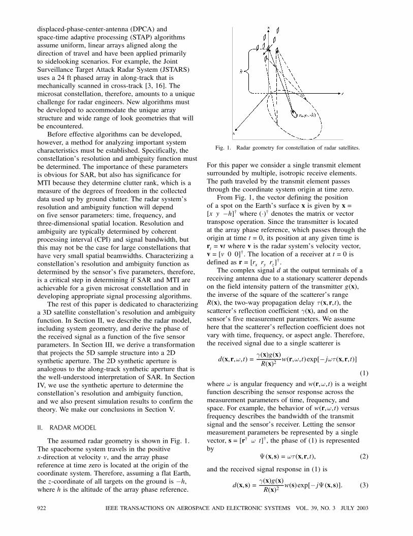
The assumed radar geometry is shown in Fig. 1.The spaceborne system travels in the positivex-direction at velocity v, and the array phasereference at time zero is located at the origin of thecoordinate system. Therefore, assuming a flat Earth,the z-coordinate of all targets on the ground is h,where h is the altitude of the array phase reference.

Fig. 1. Radar geometry for constellation of radar satellites.

For this paper we consider a single transmit elementsurrounded by multiple, isotropic receive elements.The path traveled by the transmit element passesthrough the coordinate system origin at time zero.

From Fig. 1, the vector defining the positionof a spot on the Earth’s surface x is given by x=[x y h]† where ( )† denotes the matrix or vectortranspose operation. Since the transmitter is locatedat the array phase reference, which passes through theorigin at time t= 0, its position at any given time isrt = vt where v is the radar system’s velocity vector,v= [v 0 0]†. The location of a receiver at t= 0 isdefined as r= [rx ry rz]

†.The complex signal d at the output terminals of a

receiving antenna due to a stationary scatterer dependson the field intensity pattern of the transmitter g(x),the inverse of the square of the scatterer’s rangeR(x), the two-way propagation delay ¿(x,r, t), thescatterer’s reflection coefficient °(x), and on thesensor’s five measurement parameters. We assumehere that the scatterer’s reflection coefficient does notvary with time, frequency, or aspect angle. Therefore,the received signal due to a single scatterer is

d(x,r,!, t) =°(x)g(x)R(x)2

w(r,!, t)exp[ j!¿(x,r, t)]

(1)

where ! is angular frequency and w(r,!, t) is a weightfunction describing the sensor response across themeasurement parameters of time, frequency, andspace. For example, the behavior of w(r,!, t) versusfrequency describes the bandwidth of the transmitsignal and the sensor’s receiver. Letting the sensormeasurement parameters be represented by a singlevector, s= [r† ! t]†, the phase of (1) is representedby

ª (x,s) = !¿ (x,r, t), (2)

and the received signal response in (1) is

d(x,s) =°(x)g(x)R(x)2

w(s)exp[ jª (x,s)]: (3)

922 IEEE TRANSACTIONS ON AEROSPACE AND ELECTRONIC SYSTEMS VOL. 39, NO. 3 JULY 2003

From (3), it is apparent that several variables affectthe phase of the received radar response due to asingle scatterer. The phase varies with sensor time,space, and frequency as well as the location of thescatterer. The only scatterer-dependent parameters thataffect how the received phase varies are the x and ycoordinates of the scatterer. Since the scatterers onlyhave two variables that affect their response at theradar, it is reasonable to assume that only two sensordimensions are needed for representing the SAR data.Therefore, the hypothesis is that although the phaseexpression of (3) varies versus five sensor parameters,those sensor parameters can be projected into thecoordinates of two independent eigensensors. Theprojection of a sensor’s time, space, and frequencyparameters onto these two eigensensors forms a 2Dsynthetic sensor that can be used to characterize SARand MTI performance. We further note that although aflat-Earth approximation has been made here, a 2Dsynthetic aperture can be generated for stationaryscatterers located on any 2D surface because onlytwo independent variables are needed to define ascatterer’s location.

III. SPACE-TIME-FREQUENCY SYNTHETIC APERTURE

The manner in which ª varies over scattererposition and sensor parameters determines resolutionand the radar ambiguity function. For sidelookingarrays with large bandwidths, long CPI lengths, andrelatively small physical arrays, the along-track andcross-track directions decouple and we understandvery well the resulting along-track and cross-trackresolutions [17]. For the microsat concept, however,this may not be the case. Even for sidelookinggeometries, if the physical array is wide enough thatthe mainlobe of the array pattern dominates resolutionrather than bandwidth and CPI length, then the twomain axes of resolution may rotate away from along-and cross-track. Furthermore, the satellite constellationmay be steered to look forward or backward. Inthis case, the size and orientation of the resolutioncell are not straightforward to determine. We needa method of predicting the ambiguity function andsize and shape of a resolution cell for a wide rangeof transmitted signals, physical arrays, and lookgeometries.In this section, we derive a method for determining

a radar system’s resolution and ambiguity function.We expand the received phase response using Taylorexpansions to demonstrate that the five sensorparameters of space, time, and frequency can beprojected into an equivalent two-dimensional sensorthat we call the 2D synthetic aperture. The 2Dsynthetic aperture is analogous to the 1D syntheticaperture interpretation of traditional SAR. In SAR,one or more receivers are placed on a movingplatform. As the platform moves over successive

samples, the measurements obtained are equivalentto a set of measurements obtained by a nonmovingarray with element spacing dependent on the pulserepetition interval (PRI); hence, time and along-trackposition are related by the sensor velocity. Moregenerally, however, we can say that two sensorparameters, time and along-track position, aretransformed into an equivalent 1D aperture. Similarly,we take five sensor parameters and project them intoa 2D synthetic aperture. The advantage is the same asfor traditional SAR. We analyze the synthetic apertureto understand the resolution and ambiguity functionof the moving radar system. Here, we use the 2Dsynthetic aperture to understand the resolution andambiguity function of a radar system that moveswith time, samples over a certain bandwidth, andhas receive elements offset in along-track and twocross-track dimensions.

A. Synthetic Aperture Derivation

First-order Taylor expansions of the phase of theradar response are performed in two steps. First, ª isexpanded around the radar sensor parameters s. Theresult is

ª(x,s) ª (x, s̄) + ( sª x,s̄)†¢s (4)

where

s̄= [rx0 ry0 rz0 !0 t0]†

s= [@=@rx @=@ry @=@rz @=@! @=@t]†

¢s= s s̄= [rx rx0 ry ry0 rz rz0 ! !0 t t0]†

:

(5)

In (4), s̄ is the set of sensor parameters around whichthe expansion is performed. Using the array phasereference, mean sensor time, and mean frequency,the sensor parameters around which the expansion isperformed are given by

s̄= [0 0 0 !0 0]†: (6)

The first term in (4) is a constant phase term withrespect to changes in the sensor parameters, ¢s. Assuch, we can assume without a loss of generality thatit is zero. The second term of (4) contains all themeasurement information about a target at x. To seethis, we explicitly write the derivatives implied by thegradient operation:

ª (x,s) =@ª

@rx x,s̄rx+

@ª

@ry x,s̄

ry +@ª

@rz x,s̄

rz

+@ª

@! x,s̄(! !0) +

@ª

@t x,s̄t: (7)

The derivatives in the first three terms show thechange of measurement phase with respect to sensor

GOODMAN & STILES: RESOLUTION AND SYNTHETIC APERTURE CHARACTERIZATION 923

position in each of three spatial directions. Theseare, by definition, the spatial frequencies kx(x),ky(x), and kz(x) of the wave scattered from a targetat x. Likewise, the fourth term provides the changein measurement phase with respect to temporalfrequency, which is the definition of the propagationdelay to the target. The final term shows the changein measurement phase as a function of time, whichdefines the target’s Doppler frequency. Recognizingthese definitions, (7) can be written as

ª(x,s) = kx(x)rx+ ky(x)ry + kz(x)rz

+ ¿(x)(! !0) +!D(x)t (8)

where kx, ky, and kz are the spatial frequencies,¿ is the delay, and !D is the Doppler frequencyassociated with the scattered signal from a target atx. Hence, we can view a radar as a sensor that collectsmeasurements across five dimensions: space, time, andfrequency, providing information about five scatteredsignal frequencies: kx, ky, kz, ¿ , and !D.Returning to (4), which was the phase function

after expanding around the sensor parameters, thesensor-dependent component of phase is written as

ª (x,s) = ks(x)†¢s (9)

where ks(x) = sª x,s̄ is used to emphasize similaritywith the standard wavenumber vector. Next, thefirst-order Taylor expansion of ks(x)

† around theposition of the scatter on the ground is performed.Defining x̄= [x0 y0 h]† as the central point ofillumination on the ground and the point aroundwhich the expansion is performed, the expansionis

ks(x)† ks(x̄)

† +¢x†[ xks(x)†x̄] (10)

where¢x= x x̄= [x x0 y y0]

† (11)

and

x = [@=@x @=@y]†: (12)

The received phase then becomes

ª (x,s) ks(x̄)†¢s+¢x†[ xks(x)

†x̄,s̄]¢s

= [(k0s )† +¢x†¤s]¢s (13)

where k0s = ks(x̄) = sª x̄,s̄, and ¤s = x( sª )†x̄,s̄ is

coined the sensor transformation matrix. In (13), k0s isa five-dimensional vector describing the center signalfrequencies. These are the average frequency values ofthe scattered signals from across the illuminated areaand correspond to the signal frequencies due to thecenter location x̄. Therefore, the second term in (13),¢x†¤s, is a vector that represents the deviation fromthe center signal frequencies, resulting from a targetlocated at x̄+¢x. The matrix ¤s thus transforms

the two-dimensional target position vector x into thefive-dimensional scattered signal frequency vector thatcorresponds to that target.

Using (13), the received signal in (3) becomes

d(x,¢s) =°(x)g(x)R(x)2

w(¢s)exp j[(k0s )†¢s+¢x†¤s¢s] :

(14)

Next, attention is turned to the radiation patterng(x) of the transmitting antenna. The transmittingantenna is a single aperture that is much smaller thanthe volume spanned by the sparse receive array. Formicrosat constellations, this corresponds to havingonly one satellite transmitting. The antenna patternis given by

g(x) =SA

wl(l) exp[ jªl(x, l)]dl: (15)

In (15), wl(l) is the antenna’s complex current or fielddistribution, l= [lx ly lz]

† is a vector to a point on theantenna’s conducting structure or aperture, SA is thesurface of the conducting structure or aperture, andªl(x, l) is the relative phase shift over the antenna dueto a slightly varying range to the scatterer location x.The phase shift ªl(x, l) is given by

ªl(x, l) =!0cl x : (16)

Since the antenna distribution wl(l) is complex, it canbe written as

wl(l) = wl(l) exp[ jªa(l)]: (17)

The phase in (15) is similar to the phase usedpreviously to derive the sensor response. The range toa point x on the scattering surface varies slightly overthe antenna structure. The radiation pattern is obtainedby integrating this variation over the antenna structureas indicated by (15). Performing Taylor expansionssimilar to those performed earlier for the sensorparameters, the phase of the antenna distribution canbe expressed as

ªl(x, l) = (k0l )†¢l+¢x†¤l¢l (18)

where

k0l = lªl x̄,l̄, (19)

¤l = x( lªl)†x̄,̄l, (20)

l = [@=@lx @=@ly @=@lz]†, (21)

¢l= l l̄, (22)

l̄ is the point on the antenna structure aroundwhich the first expansion is performed, and ¤l istermed the antenna transformation matrix. Using (18),


the transmit pattern is

g(x) =SA

wl(l) exp j[ªa(l)+ (k0l )†¢l+¢x†¤l¢l] dl:

(23)

Last, the transmitting antenna can be focused on themean scatterer location x̄ by forcing a phase taper of

ªa(l) = (k0l )†¢l: (24)

Then, the transmit pattern is

g(x) =SA

wl(l) exp( j¢x†¤l¢l)dl: (25)

B. Synthetic Aperture Interpretation

The performance of a traditional, single-aperture,sidelooking SAR is relative easy to evaluate andunderstand. a target’s position in cross-track isdetermined from the signal delay, while its along-trackposition is determined by Doppler. Moreover, thecross-track resolution is determined by the frequencybandwidth of the transmit signal, and the along-trackresolution is determined by the processing timewidth,or CPI.Alternatively, the behavior of proposed

sparse-array radars appears difficult to evaluate. Thesesensors, in general, will not be sidelooking, andthe spatial extent of the satellite array can be largeenough to affect sensor resolution. As a result, allfive signal frequencies may be jointly dependent onboth the along-track and cross-track positions of thetarget. This complex coupling between target positionand scattered signal frequencies is demonstrated bythe sensor transformation matrix ¤s. In general, allelements of this matrix will be non-zero, showing thateach signal parameter is dependent on each dimensionof target position. Accordingly, the sensor providesalong-track and cross-track resolutions that are bothjointly dependent on frequency bandwidth, CPI, andthe spatial size of the 3D array. Resolution will bedetermined by some or all of these parameters, asopposed to just one. Moreover, resolution will be afunction of look angle, so that there exists no simple,direct relationship between sensor resolution andsensor bandwidth, CPI, and array size.However, analysis of the sensor transformation

matrix provides a method for projecting the fivesignal frequencies and five sensor measurementsinto a two-dimensional space. We find that theseprojections are orthogonal, such that each projectedmeasurement corresponds to target position in oneof two orthogonal directions. In this manner, atwo-dimensional synthetic aperture is constructed fromthe original five-dimensional set of measurements.

To create this synthetic aperture, we begin byexpressing the sensor transformation matrix in termsof its singular value decomposition (SVD), given by

USV† =¤s (26)

where

U= [u1 u2] (27)

S=¾1 0 0 0 0

0 ¾2 0 0 0(28)

andV= [v1 v2 v3 v4 v5]: (29)

Then, with the SVD explicitly expanded, the receivedphase is

ª(x,s) (k0s )†¢s+¾1(¢x

†u1)(v†1¢s) +¾2(¢x

†u2)(v†2¢s)

= (k0s )†¢s+ k®®+ k¯¯ (30)

where k® = ¾1¢x†u1, k¯ = ¾2¢x

†u2, ®= v†1¢s, and

¯ = v†2¢s. The sensor transformation matrix can beinterpreted using (30). The basis vectors, v1 and v2,for the rows of ¤s project the five sensor parametersinto two independent dimensions of a 2D syntheticaperture, ® and ¯. Based on their interpretationusing eigenanalysis, the two dimensions are termedeigensensors. The first eigensensor is obtained throughthe inner product of the sensor parameter vector¢s with v1, and the second eigensensor is obtainedthrough the inner product of the sensor parametervector ¢s with v2. Consequently, the coordinatesof an element in the synthetic aperture are given by®= v†1¢s and ¯ = v

†2¢s. When these two dimensions

are used as the measurement dimensions, then theyare the only two dimensions needed because theyare the only two dimensions with non-zero singularvalues. The other three dimensions: v3, v4, and v5, areassociated with zero singular values, and a change inthe position of a scatterer produces no change in themeasurements obtained in these three dimensions.Therefore, only the first two dimensions provideinformation about stationary scatterers, and these twodimensions preserve all the information collected bythe sensor in space, time, and frequency.

In addition to preserving all the sensor informationin just two dimensions, the two eigensensors arealso independent. Therefore, the two eigensensorsprovide information about two orthogonal frequenciesthat are obtained through inner products with thebasis vectors, u1 and u2 for the columns of ¤s. Thevalues of the new spatial frequencies are given byk® = ¾1¢x

†u1 and k¯ = ¾2¢x†u2.

The eigensensors provide the opportunity tocharacterize radar behavior with the same simplicityas with standard, sidelooking SAR. Just as signaldelay and Doppler correspond, respectively, to target


cross-track and along-track position, the signalfrequencies k® and k¯ correspond, respectively,to target position in orthogonal directions u1 andu2. Also, just as target resolution in cross-trackand along-track depend, respectively, on sensorbandwidth and CPI, target resolution in u1 and u2depend, respectively, on the extent, or width, of sensormeasurements ® and ¯.Note that for an individual antenna, ¤l performs a

function similar to what ¤s performs for the sensorsamples. ¤l takes any point on the structure of anantenna and projects that point onto a plane. Theplane is perpendicular to boresight of the antenna asdefined by x̄. Therefore, the antenna transformationmatrix ¤l takes an antenna aperture described in3D space and transforms it into a 2D antenna thathas an equivalent illumination pattern for the regionsurrounding the point x̄. In addition, ¤l projectsthe original spatial frequencies corresponding tothe x and y positions of the scatterer to new spatialfrequencies that are measured by the primary axes ofthe equivalent 2D antenna.

C. Sidelooking Example

Although the SVD of ¤s must generally beperformed numerically, a sidelooking sensor geometryprovides a case where algebraic expressions of theSVD can be determined. The results describe theknown behavior of a sidelooking SAR, and providesupport to both the validity and utility of this method.From the geometry and vectors defined earlier, therange from the transmitter to a scatter at x is given by

Rtx = rt x = (vt x)2 + y2 + h2: (31)

Likewise, the range from the scatterer back to areceiver is given by

Rrx = r+ vt x = (rx+ vt x)2 + (ry y)2 + (rz + h)2

(32)and the two-way propagation delay is

¿(x,r, t) =1c

(rx+ vt x)2 + (ry y)2 + (rz +h)2

+ (vt x)2 + y2 +h2 : (33)

In terms of derivatives, ¤s is given by

¤s =

@2

@x@rx

@2

@x@ry

@2

@x@rz

@2

@x@!

@2

@x@t

@2

@y@rx

@2

@y@ry

@2

@y@rz

@2

@y@!

@2

@y@t

ª

x̄,s̄

:

(34)

Substituting (33) and (2) into (34) and evaluating at s̄and x̄, the sensor transformation matrix becomes

¤s=!0c

(h2 + y20)

R30

x0y0R30

x0h

R30

2x0!0R0

2v(h2 + y20)

R30

x0y0R30

(h2 + x20)R30

y0h

R30

2y0!0R0

2vx0y0R30

(35)

where R0 = h2 + x20 + y20. For sidelooking, x0 = 0,

and ¤s becomes

¤s =

1R0

0 0 02vR0

0h2

R30

y0h

R30

2y0!0R0

0: (36)

Substituting (36) back into (13), the phase response is

ª(x,s) = (k0s )†¢s+

!0c(y y0)

2y0!0R0

(! !0)h2

R30ry

y0h

R30rz

!0c

x

R0(rx+2vt) (37)

and (14) becomes

d(x,¢s)

=1

R(x)2w(¢s)exp[ j(k0s )

†¢s]

exp j!0c(y y0)

2y0!0R0

(! !0)h2

R30ry

y0h

R30rz

exp j!0c

x

R0(rx+2vt)

SA

wl(l) exp( j¢x†¤l¢l)dl: (38)

Looking at (38), it is seen that the along- andcross-track dimensions contribute independentcomponents. In (38), the first line contains theattenuation due to spreading and the measured phasedue to the mean target frequencies. The secondline describes the cross-track component, the thirdline describes the along-track component, and thefourth line accounts for the radiation pattern of thetransmitter. Isolating the along-track component andnoting that !0x=cR0 kx, the along-track component is

½x = exp[kx(rx+2vt)]: (39)

Equation (39) is the along-track responsecommonly used in SAR and MTI analysis. It showsthat the along-track spatial frequency componentis sampled by a synthetic aperture with elementslocated at (rx+2vt). Consequently, (13) is awardeda degree of confidence based on proper prediction ofthe along-track component for the sidelooking case.Simulations presented later in this paper demonstratethat (13) is valid for a wide span of scenarios.


IV. SENSOR RESOLUTION AND AMBIGUITYFUNCTION

Now that (13) provides a method for projectingall sensor parameters into a synthetic 2D aperture,it is straightforward to evaluate the radar system’sresolution and ambiguity function. The beampatternof the resulting synthetic aperture can be determinedin the same manner as any physical aperture, albeitwith results in terms of spatial frequencies k® andk¯ . The resulting pattern can be directly projectedonto an illuminated surface, along the coordinatesystem defined by u1 and u2. This projectionresults in the function commonly referred to as thesensor’s ambiguity function and effectively displaysthe correlation of one target’s response with theresponse from targets at all other locations. Thesensor characteristics that can be discerned fromthis function include resolution and target ambiguity,where target ambiguity is manifested as grating lobesand sidelobes.In the first part of this section, expressions

are derived that define the resolution of sparseradar arrays. The efficacy of these expressions isdemonstrated by comparing their predictions withambiguity functions generated from a numeric radarsimulator. In the latter section, measurement ambiguityin the form of both grating lobes and sidelobes isaddressed.

A. Resolution

Radar resolution is traditionally considered interms of the correlation between two adjacent targets.This correlation can, of course, be expressed in termsof a matched-filter response; therefore, we begin thisanalysis by determining the output of a matched filterin the presence of two targets. The filter is matchedto the first signal, which is due to a target at x= x̄.Initially, we assume that the transmit aperture has aGaussian amplitude taper with size and orientationdescribed by the matrix Jl and phase taper accordingto (24), such that

wl(l) =1

(2¼)3=2 Jlexp[ 1

2¢l†J 1l ¢l]exp[j(k

0l )†¢l]:

(40)

The received signal due to a scatterer at x̄ with ascattering coefficient of °1 is

d1(x̄,¢s) =°1R(x̄)2

w(¢s) exp[ j(k0s )†¢s]

1

(2¼)3=2 Jlexp[ ¢l†J 1

l ¢l]d¢l

=°1R(x̄)2

w(¢s) exp[ j(k0s )†¢s]g(x̄): (41)

The received signal due to a second scatterer locatedat x̄+¢x with a scattering coefficient of °2 is

d2(x̄+¢x,¢s)

=°2

R(x̄+¢x)2w(¢s)exp[ j(k0s )

†¢s]

exp[ j¢x†¤s¢s]

SA

1

(2¼)3=2 Jlexp[ 1

2¢l†J 1l ¢l]

exp[ j¢x†¤l¢l]d¢l: (42)

By completing the square in the integrand of (42), d2is

d2(x̄+¢x,¢s)

=°2

R(x̄+¢x)2w(¢s)exp[ j(k0s )

†¢s]

exp[ j¢x†¤s¢s]

g(x̄) exp[ 12¢x

†¤lJl¤†l¢x]: (43)

A filter matched to the response from the first targetcan be implemented by correlating with the functionhc given by

hc =R(x̄)2

g(x̄)w(¢s) exp[j(k0s )

†¢s]: (44)

We assume also that the sensor weight function w(¢s)is Gaussian with width and orientation described bythe covariance matrix Js. Although this assumptionappears to be restrictive and unrealistic, we showthat this Gaussian assumption leads to a result that isalso very accurate for other sensor weight functions.Therefore, the sensor weight function, w(¢s), isexpressed as

w(¢s) =1

(2¼)5=4 Js 1=4exp( 1

4¢s†J 1s ¢s): (45)

The output » of the correlation filter is

» =S

(d1 + d2 + ni)hcd¢s

= °1S

w(¢s) 2d¢s

+ °2R(x̄)2

R(x̄+¢x)2exp[ 1

2¢x†¤lJl¤

†l¢x]

S

w(¢s) 2 exp[ j¢x†¤s¢s]d¢s+ no

(46)

where ni and no are additive Gaussian noise at theinput and output of the filter, respectively, and theintegrations are performed over the full range of eachsensor measurement parameter. The first term in (46)is simply an integration over a 5D Gaussian function;therefore, the integral goes to one and the first termbecomes the desired output, °1. Since the filter is


matched to the first scatterer, the second term in (46)depends on the correlation between d1 and d2. Thesecond term, which is temporarily designated as»2, is

»2 = °2R(x̄)2

R(x̄+¢x)2exp( 1

2¢x†¤lJl¤

†l¢x)

exp( 12¢x

†¤sJs¤†s¢x): (47)

Noting thatR(x̄)2

R(x̄+¢x)21 (48)

when ¢x is small, the output of the correlation filterbecomes

» = °1 + °2 exp[12¢x

†(¤sJs¤†s +¤lJl¤

†l )¢x] + no:

(49)

Equation (49) shows that the output of the correlationfilter depends on three terms. The first term is thedesired output—the reflectance due to the pixel ofinterest. The second term is the error due to leakageof the second target into the filter output. It dependson the exponential term, which we now recognize asthe correlation between the two scatterers. The lastterm is the error due to noise that passes through thematched filter.1) Resolution Defined by Target Correlation: We

use two criteria for defining sensor resolution. Thefirst uses the more traditional approach where twotargets are resolvable if their responses are sufficientlyuncorrelated. From (49), the correlation between theresponses of targets located at x̄ and x̄+¢x is

∙c = exp[12¢x

†(¤sJs¤†s +¤lJl¤

†l )¢x]: (50)

We can use this expression to determine thecorrelation between two targets displaced by ¢x,or we can fix the correlation ∙c to a specified valueand determine the locations of all targets that arecorrelated by the same amount. Taking the naturallogarithm of (50), we get elliptical contours ofconstant correlation defined by

2ln∙c =¢x†(¤sJs¤

†s +¤lJl¤

†l )¢x: (51)

If the constant ∙c represents the correlation requiredfor target resolution, then the resulting contour canbe considered the resolution ellipse, a contour thatindicates both the size and orientation of the mainlobeof the sensor ambiguity function. The size of theellipse depends on both the value of ∙c and on theresulting matrix in parentheses. For example, thesize of the ellipse depends inversely on the matrix’sdeterminant. If the sensor’s measurement extent isincreased (e.g., its bandwidth and/or CPI is increased),the variances in Js become larger, and the determinantof the matrix increases. As a result, the resolution

ellipse decreases in size, indicating an expectedimprovement in sensor resolution.

Typically, the transmit antenna does not impactradar sensor resolution. Accordingly, the determinantof ¤lJl¤

†l is relatively small, and (51) can be

approximated as

2ln∙c =¢x†¤sJs¤

†s¢x: (52)

2) Resolution Defined by Estimation Error:The second approach to resolution is based on theCramer–Rao lower bound (CRLB). The matched filteroutput value » can be used to estimate the complexreflection coefficient °1. Due to measurement noiseand the presence of a second target with unknownreflectance °2, this estimate will exhibit error thatdepends on the estimator implemented. The CRLB,however, provides a lower bound on the error varianceproduced by any unbiased estimator.

We begin by determining the Fisher informationmatrix [18], defined as

J= E [ °(lnp(» °))][ °(lnp(» °))]† : (53)

Given that the noise and complex target reflectancescan be accurately described as independent Gaussianrandom variables, J is determined to be

J=

1¾2n+1¾2°

∙c¾2n

∙c¾2n

∙2c¾2n+1¾2°

(54)

where E[ °12] = E[ °2

2] = ¾2° , E[°1°2] = 0, andE[ no

2] = ¾2n . The CRLB is contained in the inverseof this information matrix,

J 1 =1

¾2n +¾2°(1+∙2c)

¾2° (¾2n +¾

2°∙2c ) ∙c¾

4°

∙c¾4° ¾2° (¾

2n + ¾

2° )

:

(55)

The lower bounds for the estimation error varianceof the two target reflectances are given on the maindiagonal of (55). Therefore, the CRLB of the errorvariance of the estimate °̂1(») is

E[ °1 °̂1(»)2] ¾2°

1+¾2°¾2n

∙2c

1+¾2°¾2n(1+ ∙2c )

∙2e : (56)

We see in (56) that the estimation error depends onthe signal-to-noise ratio (SNR) through the ratio¾2°=¾

2n .From (56), the target correlation in terms of the

CRLB is

∙2c =¾2°¾

2n ∙2e¾

2° ∙2e¾

2n

¾2° (∙2e ¾2° ): (57)


Inserting (50) into (57), we form the followingrelationship:

ln¾2°¾

2n ∙2e¾

2° ∙2e¾

2n

¾2° (∙2e ¾2° )=¢x(¤sJs¤s+¤lJl¤l)¢x:

(58)For a desired value of estimate error variance,

∙2e , the above expression can be solved for ¢x.The set of all such solutions can be used to mapcontours of equal error variance, which again willbe elliptically shaped. Therefore, (51) and (58) eachdefine a resolution ellipse, providing a graphicalindication of sensor resolution. Equation (51) usestarget correlation as the resolution criterion whereas(58) uses estimation error variance. Although thetarget correlation is the more traditional criterion, (58)uses a criterion more directly dependent on sensorparameters, specifically SNR and desired estimateerror variance.3) Simulations: Using (51), we have predicted

the resolution ellipses for several cases and comparedthem with ambiguity functions obtained numericallyusing a multiple aperture radar simulator. The numericsimulator was developed in-house. It computes thein-phase and quadrature analog-to-digital convertersamples for a scatterer at a given location x. Thesamples are computed for every array element,slow-time sample, and frequency (fast-time)sample. The sets of measurements due to allilluminated scatterers can be weighted by theircorresponding scattering reflectivities and summedto obtain a simulated version of the complete radarmeasurements. Then, the radar measurements canbe input into a SAR or MTI processor. In addition,the data samples from each scattering location canbe correlated to arrive at a numerically generatedambiguity function. a more detailed description of thesimulator is available in [19].In the first three cases that follow, Gaussian

tapers were used for the time and frequency sensordimensions. a uniform taper, however, was appliedacross the physical array, with the spatial-dependentelements of Js calculated according to a variancemeasure of the sparse array. For example, the (x,y)component of Js, J

xys , was calculated according to

Jxys =S

(rx rx0)(ry ry0)drxdry: (59)

In the fourth example, all five sensor parameters haduniform tapers with elements of Js calculated in amanner equivalent to (59).Fig. 2 shows a sidelooking scenario with a sparse,

but relatively small, physical array. The physical arrayin this case is small enough that the transmit signal’sbandwidth and CPI length are the dominant factorsin determining resolution. The 2D and 3D viewsare shown in Figs. 2(a) and 2(b), respectively. Theresolution ellipse, shown as black in the 3D view

Fig. 2. Simulated ambiguity function and theoretically predictedresolution ellipse for a sidelooking geometry with small physical

array. (a) 2D view. (b) 3D view.

and white in the 2D view, is correctly predicted withits axes aligned with the along-track and cross-trackdirections. The resolution axes align with the along-and cross-track dimensions in this case becauseresolution is controlled by bandwidth and CPI length.From the 3D view, it is seen that the predictedresolution ellipse intersects the numerical ambiguityfunction at approximately the specified correlationlevel, which was ∙c = 0:707.

When the physical array is extremely large,however, the result is as seen in Fig. 3. In thiscase, the ellipse becomes smaller because the arraybeamwidth is smaller than the resolution providedby the sensor’s bandwidth and CPI. Moreover, eventhough the scenario is still sidelooking, the axes ofthe resolution ellipse rotate away from along- andcross-track because the array formed by the satelliteconstellation has no along- and cross-track symmetry.In addition, since the physical array is the dominantcomponent and it is sparsely populated with auniform taper, the sidelobes in the ambiguity function


Fig. 3. Simulated ambiguity function and theoretically predictedresolution ellipse for sidelooking geometry with large physical

array that affects resolution. (a) 2D view. (b) 3D view.

are much larger in Fig. 3 than they were inFig. 2.In Fig. 4, the physical array is again relatively

large, but now the scenario is forward looking. Theresolution ellipse’s size and orientation are correctlypredicted by (51). The axes of the resolution ellipsedo not align with along- and cross-track because ofthe forward-looking geometry and the orientationof the satellite array. Sidelobes are again significantbecause the dominant sensor measurements thatdetermine the mainlobe shape and size are themeasurements obtained by the sparse, uniformlyweighted, satellite array.Last, we demonstrate in Fig. 5 that the Gaussian

assumption made in deriving (51) is not as restrictiveas it may appear. In the simulations that produced Fig.5, each of the five sensor measurement parameters:time, frequency, and 3D space, were given uniformamplitude tapers. The elements of Js were calculatedaccording to the variance of the uniform tapers, asdemonstrated for the (x,y) component in (59). The

Fig. 4. Simulated ambiguity function and theoretically predictedresolution ellipse for forward-looking geometry with large physical

array that affects resolution. (a) 2D view. (b) 3D view.

scenario is forward looking with a moderately sizedconstellation. Therefore, all five sensor parameters hadan effect on total system resolution. The results shownin Fig. 5 demonstrate that by using the variance ofthe uniform tapers, the resolution of the system canstill be determined effectively. Furthermore, sincemany realistic frequency spectra, time windows, andarray functions are closer in shape to a Gaussian taperthan to a uniform taper, we conclude that the Gaussianassumption used to derive (51) does not significantlyrestrict the range of scenarios or sensor functions towhich (51) can be applied.

B. Sensor Ambiguity Function

In addition to resolution, a fundamentalperformance characteristic of a sparse radar arrayis the sidelobe structure exhibited in the sensorambiguity function. At a minimum, no grating lobes,which result from perfect measurement correlationbetween dissimilar targets, should occur within the


Fig. 5. Simulated ambiguity function and theoretically predictedresolution ellipse for forward-looking geometry with moderatelysized physical array that affects resolution. Uniform tapers applied

to all five sensor measurement parameters. (a) 2D view.(b) 3D view.

sensor ambiguity function. In addition, the sidelobesof the ambiguity function should ideally be small.Again considering the traditional sidelooking,single-aperture SAR, significant sidelobes within thesensor ambiguity function can be directly determinedfrom knowledge of the transmit pulse repetitionfrequency (PRF). However, for a sparse radar array,the concept of the synthetic aperture, as discussedin Section III, must be implemented to determinesensor ambiguity. The complexity of this sensor:five sensor measurement parameters, forward- andbackward-looking geometries, and the large but sparsespatial array, make a more direct analysis problematic.For the analysis in this section, we assume the

radar transmits a simple coherent pulse train at aconstant PRF. As a result, the sensor weight functionfor the time parameter wt(¢t) is represented as aperiodic series of time samples separated by 1/PRFacross the sensor’s CPI. Similarly, the weight function

for the frequency parameter wf(¢!) is represented asa periodic series of frequency samples separated by2¼PRF across the sensor bandwidth. Since the receivearray formed by the satellite constellation likewiserepresents sampling in three dimensions of space,the entire sensor weight function w(¢s) representsa five-dimensional array. This array can be then beprojected into a two-dimensional synthetic array, usingthe projection vectors described in Section III.

As stated earlier, the sensor ambiguity functionfor a sparse radar array is determined from thetwo-dimensional synthetic aperture or array, asdescribed in Section III. As with any aperture orarray, the sidelobe levels of the resulting patterndepend on the aperture function since the two arerelated by a Fourier transform. As a result, the2D synthetic aperture function of a sparse radararray can provide direct insight into the behaviorof this sensor. For example, the size of the aperturein each orthogonal measurement direction willdetermine sensor resolution. Likewise, to avoid largesidelobes, the aperture or array must be filled—that is,measurements must be made across the entire apertureextent. Additionally, grating lobes can occur if thesynthetic aperture or array has periodicities.

More specifically, to evaluate the sidelobeperformance of a synthetic array, the concept of acoarray is used. The coarray is the autocorrelation ofthe array and is a measure of the spatial lags sampledby the array. The far-field power pattern produced byan array is simply the Fourier transform of its coarray.Regularly spaced arrays and coarrays are defined ashaving spacing that can be laid out on an underlying,evenly spaced grid. Therefore, the distances betweensamples are always multiples of each other. If samplesare missing such that the Nyquist criterion is notsatisfied, the array is said to be sparsely populated.If no underlying grid can be found on which to locatethe samples, then the array is said to be randomly, ornon-uniformly, spaced.

There are two cases where true grating lobes donot occur: when a regularly spaced coarray is Nyquistsampled or when the coarray is irregularly spaced. Ifa regular coarray results in grating lobes, then theirseparations from the mainlobe are determined bythe minimum separation between coarray samples.Therefore, a regularly spaced, sparse array will nothave true grating lobes if some of its coarray samplesare closely spaced. For an irregular coarray, highsidelobes are possible, but the lack of a periodicstructure prevents true grating lobes. Therefore,a sparse array radar system based on the satelliteconstellation concept will not likely have true gratinglobes, although high sidelobes could be present. Forrandomly placed arrays such as we have assumedfor microsat constellations, the number of aperturesin the array strongly controls sidelobe levels. Thisis because by adding more apertures within the


Fig. 6. Comparison of (a) numerically generated ambiguityfunction with (b) ambiguity function generated using synthetic

array.

same constellation area, the sample density of thesynthetic array is increased and the result is a moreappropriately sampled system. a more detaileddiscussion of coarrays is available in [20].First, we demonstrate in Fig. 6 that the synthetic

array derived in Section III does, indeed, accurately

Fig. 7. (a) 2D synthetic array for relatively small constellation generates synthetic coarray in (b). Ambiguity function of system shownin (c).

predict the sensor’s ambiguity function. We generatedambiguity functions for a forward-looking scenariowith both our numeric radar simulator and thesynthetic array. The ambiguity function obtainedfrom the simulator is shown in Fig. 6(a), and theambiguity function obtained from the synthetic arrayis shown in Fig. 6(b). There are some differences inthe ambiguity functions since the approximationsmade in deriving the synthetic array do not apply tothe numerical simulation. Specifically, we see thatthe differences are more apparent at the edges of theambiguity function. This is because these regions arefurther from the center of the illuminated area wherethe second Taylor expansion was performed. However,although there are some differences, the ambiguityfunctions in Fig. 6a and 6b are generally in goodagreement.

Figs. 7 and 8 demonstrate the application of thesynthetic coarray. In Fig. 7(a), the 2D synthetic arrayfor a system with a five-element satellite constellationis shown; hence, Fig. 7(a) shows the projection ofevery physical array element, slow-time sample, andfast-time sample into the 2D eigensensor system.Some periodic samples along dimension ® can beseen. These are due to periodic slow-time samples.Likewise, the periodic samples that are seen alongdimension ¯ are due to periodic fast-time samples.Additional nonperiodic samples in Fig. 7(a) are due torandom array-element spacings projected onto the 2Deigensensor.

In this example, the size of the constellation isrelatively small compared with the synthetic aperturespanned by the eight fast-time and eight slow-timesamples. Hence, many of the synthetic array samplesoverlap, and bandwidth and CPI rather than the size ofthe constellation primarily determine the overall sizeof the synthetic array. By taking the autocorrelationof the synthetic array, we generate the syntheticcoarray shown in Fig. 7(b). Because of the randomnature of the spatial sampling, there is no underlyingsample grid for either the synthetic array or coarray.Therefore, the corresponding ambiguity functionshown in Fig. 7(c) has no true grating lobes.


Fig. 8. (a) 2D synthetic array for relatively large constellation generates synthetic coarray in (b). Ambiguity function of system shownin (c).

The random-array ambiguity function, however,does show effects of both the periodic sampling ofthe radar signal and the sparse, nonperiodic samplingof the satellite constellation. Since there is periodicsampling in both time and frequency, there arehints of range-Doppler ambiguities in the resultingambiguity function. The potential range-Dopplerambiguities are multiplied by sidelobes of the radarconstellation’s radiation pattern to arrive at thesidelobes seen in Fig. 7c. Since the array patternis random in nature, the expected sidelobe levelsdepend on the sample density in the synthetic arrayand coarray [20]. This density, in turn, depends on thesystem PRF, the overall size of the constellation, andthe number of satellites in the constellation.In Fig. 8, we present the results of a final

experiment to demonstrate the effect of sample densityon the system ambiguity function. The constellationused to generate the results shown in Fig. 7 wasrelatively small. As a result, many elements of thesynthetic array overlapped, the size of the syntheticarray was primarily determined by the transmitsignal, the density of samples in the synthetic coarraywas relatively high, and the sidelobes immediatelysurrounding the ambiguity function’s mainlobe weresmall. In Fig. 8, however, the satellite constellation ismuch larger. As a result, the synthetic coarray shownin Fig. 8(a) has wide regions without any samples.The overall size of the synthetic array has increasedbecause of the huge size of the constellation, but thesample density seen in the synthetic coarray of Fig.8(b) is much less than the density seen in Fig. 7(b).Hence, although resolution has improved throughthe wider extent of the synthetic array, the reducedsampling density results in high sidelobes immediatelysurrounding the ambiguity function’s mainlobe. Theambiguity function for this case is shown in Fig. 8(c).The compromise between resolution and sample

density is a primary issue for processing of sparseradar arrays. Of course, we desire a high sampledensity over a wide extent, resulting in goodresolution and low sidelobe levels, but this may notbe achievable. We can, however, use the simulations

in Figs. 7 and 8 to make some judgments aboutwhen sparse arrays can be effectively processed forSAR and MTI. The situation in Fig. 8 is one whereresolution has improved through the large size of theconstellation. In essence, the number of resolutioncells in the SAR map has increased, but the numberof measurements for estimating the scattering fromthose cells has remained constant. Therefore, wecannot expect to be able to perform SAR processingeffectively. If, however, we design a system suchthat bandwidth and CPI are the dominant factorsin determining resolution, we ensure a sufficientsampling density such that quality SAR processingis achievable. In other words, the synthetic coarrayanalysis shows that since the time and frequencymeasurement dimensions are more sufficientlysampled than the spatial measurement dimensions,they should be the dimensions that largely determineresolution. For extremely wide satellite constellations,this may require very long CPIs and wide signalbandwidths.

V. CONCLUSIONS

There is currently an emphasis on movingradar technology into space, and one proposedconcept for doing so is a cooperative constellationof formation-flying micro-satellites. Althoughthere are many advantages to the microsat concept,current signal processing algorithms are, in general,not applicable due to the constellation’s sparselypopulated physical array. Furthermore, little effortis reported in the literature for dealing with sparselysampled, irregularly spaced, physical arrays forapplication to SAR and MTI.

To develop appropriate signal processingalgorithms, the ability to describe a radar system’simportant characteristics is needed. To that end, wehave derived a method for quickly and efficientlydetermining a radar system’s resolution and ambiguitycharacteristics. The technique transforms a radar’sfull sensor parameters: time, frequency, and spatialposition, into a two-dimensional synthetic aperture.


The synthetic aperture’s overall size determinesits mainlobe width and, therefore, the total systemresolution. Also, the synthetic aperture can be usedto generate a synthetic coarray that can be used forambiguity and sidelobe analysis.A significant advantage of this sensor

representation is that it is robust for both forward- andsidelooking scenarios and for both large and smallphysical arrays. The analysis is valid for fully filledphysical arrays as well as sparse arrays. However,since the derivation is based on Taylor expansions,far-field and narrowband conditions are assumed.While these assumptions may be restrictive forvery large physical arrays and bandwidths, we havedemonstrated through simulation that the syntheticarray can be valid for systems where the physicalarray beamwidth controls resolution rather thanbandwidth and coherent integration time. Therefore,based on the 2D synthetic aperture’s ability to predictsystem characteristics over a wide range of sensorstructures and look geometries, the method presentedin this paper should be a valuable tool for analyzingthe performance of radar systems that extend beyondairborne, sidelooking scenarios.

REFERENCES

[1] Scott, W. B. (1999)Testbeds wring out technologies.Aviation Week and Space Technology, (Apr. 5, 1999),52–53.

[2] Whelan, D. A. (2000)DISCOVERER II program summary.In Proceedings of the IEEE 2000 International RadarConference, Washington, D.C., 7–8.

[3] Entzminger, J., Fowler, C., and Kenneally, W. (1999)JointSTARS and GMTI: Past, present and future.IEEE Transactions on Aerospace and Electronic Systems,35, 2 (Apr. 1999), 748–761.

[4] Davis, M. E. (2000)Technology challenges in affordable space based radar.In Proceedings of the IEEE 2000 International RadarConference, Washington, D.C., 18–23.

[5] Proceedings of the IEEE 2001 Radar Conference, Atlanta,GA, May 1–3, 2001.

[6] Overman, K., Leahy, K., and Fritsch, R. J. (2000)The future of surface surveillance—revolutionizing theview of the battlefield.In Proceedings of the IEEE 2000 International RadarConference, Washington, D.C., 1–6.

[7] Nohara, T. J., Weber, P., and Premji, A. (2000)Space-based radar signal processing baselines for air, landand sea applications.Electronics & Communication Engineering Journal, 12, 5(Oct. 2000), 229–239.

[8] Zetocha, P., et al. (2000)Commanding and controlling satellite clusters.IEEE Intelligent Systems, 15, 6 (Nov. 2000), 8–13.

[9] Kitts, C., et al. (1999)Emerald: A low-cost spacecraft mission for validatingformation flying technologies.In Proceedings of the 1999 IEEE Aerospace Conference,Aspen, CO, 217–226.

[10] Massonnet, D., et al. (2000)A wheel of passive radar microsats for upgrading existingSAR projects.In Proceedings of the IEEE 2000 International Geoscienceand Remote Sensing Symposium, Honolulu, HI,1000–1003.

[11] Massonnet, D. (2001)Capabilities and limitations of the interferometriccartwheel.IEEE Transactions on Geoscience and Remote Sensing, 39,3 (Mar. 2001), 506–520.

[12] Air Force Research Lab (c. 1999)TechSat 21 next generation space capabilities.Available:www.vs.afrl.af.mil/TechProgs/TechSat21/NGSC.html.

[13] Martin, M., and Stallard, M. (1999)Distributed satellite missions and technologies—TheTechSat 21 program.In Proceedings of the AIAA Space Technology Conferenceand Exposition, Albuquerque, NM, Sept. 1999, AIAA99–4479.

[14] Das, A., Cobb, R., and Stallard, M. (1998)TechSat 21: A revolutionary concept in distributed spacebased sensing.In Proceedings of the AIAA Defense and Civil SpacePrograms Conference and Exhibit, Huntsville, AL, Oct.1998, AIAA 98–5255.

[15] Burns, R., et al. (2000)Techsat 21: Formation design, control, and simulation.In Proceedings of the 2000 IEEE Aerospace Conference,Big Sky, MT, 19–25.

[16] Covault, C. (1996)Joint-Stars patrols Bosnia.Aviation Week and Space Technology, (Feb. 19, 1996),44–49.

[17] N. Levanon (1988)Radar Principles.New York: Wiley, 1988.

[18] Van Trees, H. L. (1968)Detection, Estimation, and Modulation Theory, Part I.New York: Wiley, 1968.

[19] Goodman, N. A. (2002)SAR and MTI processing of sparse satellite clusters.Ph.D. dissertation, Dept. of Electrical Engineering andComputer Science, University of Kansas, Lawrence,2002.

[20] Johnson, D. H., and Dudgeon, D. E. (1993)Array Signal Processing: Concepts and Techniques.Englewood Cliffs, NJ: Prentice-Hall, 1993.


Nathan A. Goodman (S’98—M’02) received the B.S., M.S., and Ph.D. degreesin electrical engineering from the University of Kansas, Lawrence, in 1995, 1997,and 2002, respectively.He is currently an assistant professor in the Department of Electrical and

Computer Engineering at the University of Arizona. From 1996 to 1998, he wasan RF systems engineer with Texas Instruments, Dallas, TX, and from 1998 to2002, he was a graduate research assistant in the Radar Systems and RemoteSensing Laboratory (RSL) at the University of Kansas. His research interests arein radar and array signal processing.Dr. Goodman was awarded the Madison A. and Lila Self Graduate Fellowship

upon returning to the University of Kansas in 1998. He was also awarded theIEEE 2001 International Geoscience and Remote Sensing Symposium InteractiveSession Prize Paper Award.

James M. Stiles (S’91—M’95—SM’97) received the B.S. degree in electricalengineering from the University of Missouri, Columbia, in 1983; the M.S. degreein electrical engineering from Southern Methodist University, Dallas, TX, in1987; and the Ph.D. degree in electrical engineering from the University ofMichigan, Ann Arbor, in 1996.From 1983 to 1990, he was a microwave systems design engineer for Texas

Instruments, and from 1990 to 1996 he was employed as a graduate researchassistant in the Radiation Laboratory at the University of Michigan. Since 1996,he has been at the University of Kansas, where he is an associate professorof electrical engineering and a member of the Radar Systems and RemoteSensing Laboratory (RSL). His research interests include radar remote sensingof vegetation, propagation and scattering in random media, ground-penetratingradar, and radar signal processing.


odyssey into space aperture characterization of …...displaced-phase-center-antenna (dpca) and...

Documents