université d'Ottawa University of Ottawa

RELATIONSHIPS BETWEEN WATER QUALITY AND STREAM INVERTEBRATE ASSEMBLAGES OF EASTERN ONTARIO AND WESTERN QUEBEC.

Benoît Lalonde

Thesis subrnitted to the School of Graduate Studies and Research

University of Ottawa in partial fulfillrnent of the requirernents for the

M.Sc. degree in the

Ottawa-Carleton Institute of Biology

Thèse soumise a é école des études supérieures et de la recherche

Université d'Ottawa en vue de l'obtention de la maîtrise es Sciences

L' l nstitut de biologie d'Ottawa-Carleton

National Library I*) of Canada Bibliothèque nationale du Canada

Acquisitions and Acquisitions et Bibliographie Services services bibliographiques

395 Wellington Street 395. nie Wellington Ottawa ON K I A ON4 Ottawa ON K I A ON4 Canada Canada

The author has granted a non- L'auteur a accordé une licence non exclusive licence allowing the exclusive permettant à la National Library of Canada to Bibliothèque nationale du Canada de reproduce, loan, distribute or sel1 reproduire, prêter, distribuer ou copies of this thesis in microform, vendre des copies de cette thèse sous paper or electronic formats. la forme de rnicrofiche/filrn, de

reproduction sur papier ou sur format électronique.

The author retains ownershp of the L'auteur conserve la propriété du copyright in this thesis. Neither the droit d'auteur qui protège cette thèse. thesis nor substantial extracts fiom it Ni la thèse ni des extraits substantiels rnay be printed or otherwise de celle-ci ne doivent être imprimés reproduced without the author's ou autrement reproduits sans son permission. autorisation.

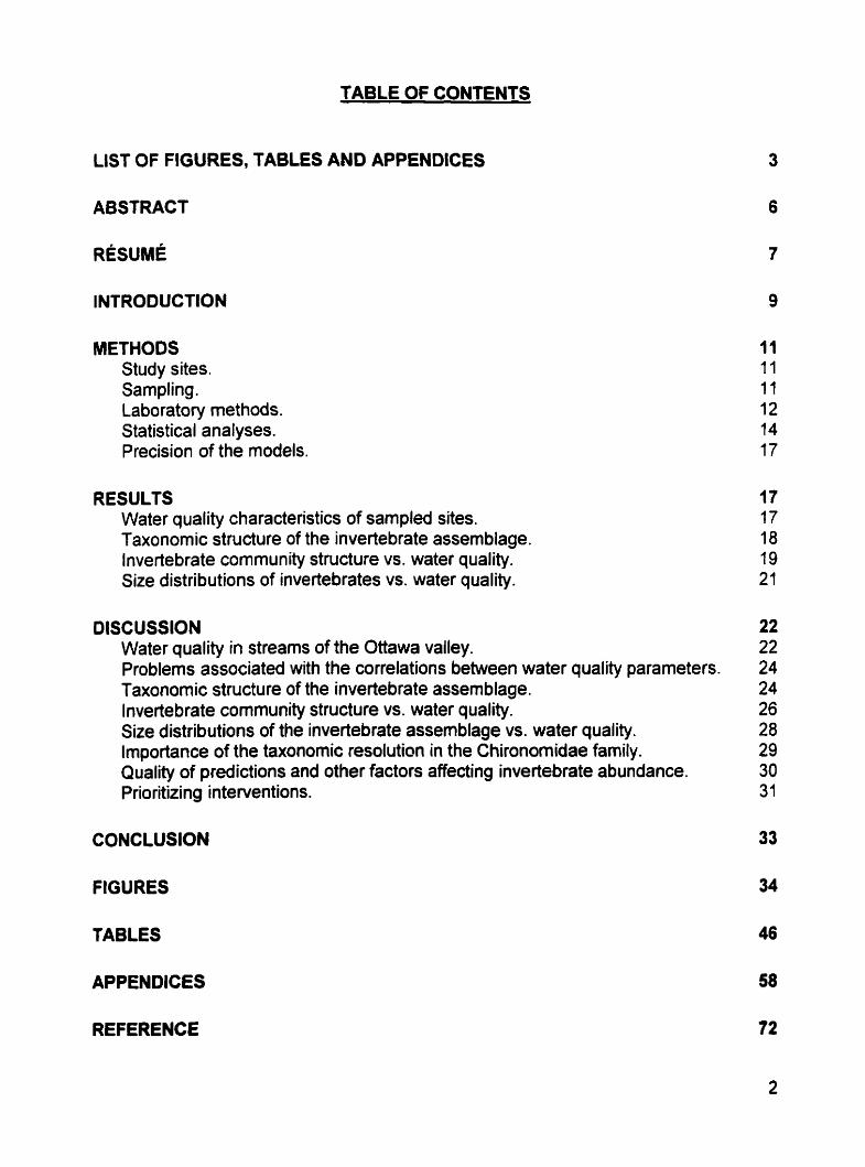
TABLE OF CONTENTS

LIST OF FIGURES, TABLES AND APPENDICES

ABSTRACT

INTRODUCTION

METHOOS Study sites. Sampling . Laboratory methods. Statistical analyses. Precision of the models.

RESULTS Water quality characteristics of sampled sites. Taxonornic structure of the invertebrate assemblage. lnvertebrate cornmunity structure vs. water quality. Size distributions of invertebrates vs. water quality.

DISCUSSION Water quality in streams of the Ottawa valley. Problems associated with the correlations between water quality parameters. Taxonornic structure of the invertebrate assemblage. lnvertebrate community structure vs. water quality. Size distributions of the invertebrate assemblage vs. water quality. Importance of the taxonomie resolution in the Chironomidae family. Quality of predictions and other factors affecting invertebrate abundance. Prioritizing interventions.

CONCLUSION

TABLES

APPENDICES

REFERENCE

Table 3. Correlation coefficients (p values) between water quality variables. Legend: Peri - (Periphyton) (mg chlalrn2), CI - Loglo (Chloride) (mglL), Conduct - Logio (Conductivity) (pslcm), NH3 - Log10 (Ammonia) (mgIL), NOx - Loglo (Nitrite and nitrate) (rnglL), SOr - Log10 (Sulfate) (mglL), SRP - Loglo (Soluble reactive phosphorus) (mg/L), TKN - Loglo (Total Kjeldahl nitrogen) (mglL), TP - Loglo

.............. (Total phosp horus) (mglL), TSS Logl (Total suspended solids) (mg/L). .51

Table 4. Multiple regression models of the principal components on taxa as a function of the principal components of water quality. Legend: PC l wQ - (chloride, sulfate. conductivity and n itrate+nitrite), PC2wa - (total suspended solids, total p hosp horus, soluble reactive p hosphorus, total Kjeldahl nitrogen, ammonia), SE - (standard error), p - (p values). n - (number of observations), R2 - (proportion of the variance

................. in the data explained by the models), RMS - (Residual mean square). 52

Table 5. Taxa richness as a function of the principal components of water quality. Legend: PCZwa - (total suspended solids, total phosphorus, soluble reactive phosphorus, total Kjeldahl nitrogen, ammonia), SE - (Standard Error), p - (p values), n - (number of observations), R2 - (proportion of the variance in the data

...... . explained by the models), RMS - (Residual mean square), PE (Pure error). 53

Table 6. Multiple regtession models of abundance per taxa as a function of water quality in strearns of the Ottawa Valley. Legend: PCIWQ - (chloride, sulfate, conductivity and nitrate+nitrite), PCZwQ - (total suspended solids, total phosphorus, soluble reactive phosphorus, total Kjeldahl nitrogen, ammonia) (SE) - (standard error), n - (number of observations), R2 - (proportion of the variance in the data explained by the models), RMS - (Residual mean square), PE - (Pure error). * = pc0.05, **=p<o .O1 , ***=p<o.o01 ......................................................................................... -54

Table 7. Multiple regression models predicting the density per size class of the total assemblage and of the dominant taxa. Legend: M-Log10 (dry mass) (pg), PClwa - (chloride, sulfate, conductivity, nitrate+nitrite), PC2wQ - (soluble reactive phosphorus, total phosphorus, total Kjeldahl nitrogen, total suspended solids, ammonia), Coeff. - (Coefficient), SE - (standard Error), p - (p value), R2 - (proportion of the variance in the data explained by the models), RMS - (Residual mean square), PE - (Pure error). ............................................................................ 55

Appendix 1. Taxon-specific intercept (a) and exponent (b) of the formula M = ~ L ~ , where M is the body mass (pg, DM) of a specific group of invertebrate and L is the body length (central axis) (in mm) ................................................................................... 58

Appendix 2. Mean Logio (density+lO) for each taxon at each sampling site. Legend: Station - (sampling station), EPH - (Ephemeroptera), PLEC - (Plecoptera), TRICH - (Trichoptera), COL - (Coleoptera). CHlR - (Chironominae), ORTH - (Orthocladiinae), TANY - (Tan ypodinae), SlMU - (Simuliidae), OlPT - (Diptera), GAST - (Gastropoda), ZEBR - (Zebra mussels), BlVA - (Bivalvia), AMPH - (Amphipoda), ISO - (Isopoda), NEM - (Nematoda), OLlG - (Oligochaeta), PLAT -

......................................... (Platyhelminthes), HYDR - (Hydra), XYZ - (unknown). 59

Appendix 3. Average logio (density +10) per size classes (mass, pg) by sampling stations (47) and by taxa (8). .................................................................................. 61

ABSTRACT

Forty-seven rime zones from 21 streams of Eastern Ontario and Western Québec were

sampled in 1998 to describe how characteristics of the benthic invertebrate assemblage

(abundance, taxa richness and size distribution) varied as a function of water quality

parameters (conductivity, TP, SRP. TSS. N03+NOî. NH3. TKN, CI-: ~ 0 ~ ~ 3 along a

gradient of watershed development. A principal cornponents analysis on water quality

parameters revealed that there were two groups of correlated water quality variables

that explained the rnajority of the variability among sites. The first group of variables

included chloride, sulfate, nitrate+nitrite and conductivity and represented a gradient of

urbanization while the second group represented nutrients and included: soluble

reactive phosphorus, total phosphorus. ammonia, total suspended solids and total

Kjeldahl nitrogen. Simple and multiple regression models predicting invertebrate

assemblage characteristics were fitted using water quality principal components scores

as independent variables. Overall, invertebrate assemblage characteristics were related

to both groups of water quality variables. Abundances per taxon and size classes

generally increased with increased nutrients. and overall abundance and the ratio of

abundances of sensitive to tolerant taxa declined with increasing chloride, sulfate,

nitrate+nitrite and conductivity. Existing information suggests that the water quality

gradient found in these streams is more a reflection of anthropogenic sources than the

result of geological differences. Therefore, it appears that human activities affect the

distribution and abundance of invertebtates in this region. However our models did not

explain a good proportion of the variability. It would seem that stream invertebrates of

the Ottawa valley are also affected by other parameters that have yet to be identified.

Quarante-sept sites situés dans les eaux rapides de 21 ruisseaux et rivières de l'Est de

l'Ontario et de l'Ouest du Québec ont été échantillonnés afin de décrire comment les

caractéristiques (abondance, richesse taxonomique et spectre de taille) des

assemblages d'invertébrés benthiques variaient en fonction de paramètres décrivant la

qualité des eaux (conductivité, TP, SRP, TSS, N03+NO~, NH3, TKN, CI*, s0d2-) le long

d'un gradient de développement des bassins hydrographiques. Une analyse par

composante principale des paramétres de la qualité des eaux a révélé qu'il y avait deux

groupes de paramètres fortement corrélés qui expliquaient une grande partie de la

variabilité entre les sites. Le premier groupe de variable représentait un gradient

d'urbanisation et comprenait le chlore, le sulfate, le nitrite+nitrate et la conductivité

tandis que le second groupe représentait un gradient d'eutrophication et comprenait le

phosphore réactif soluble, le phosphore total. l'ammoniac, les solides en suspension et

l'azote totale de Kjeldahl. Des modèles de régression simples et multiples ont été

ajustés en utilisant les scores des composantes principales de la qualité des eaux

comme variables indépendantes. Les caractéristiques de l'assemblage des invertébrés

sont généralement affectées par les deux composantes principales de la qualité des

eaux. L'abondance par taxon et par classe de taille augmentent avec une augmentation

des éléments nutritifs tandis que l'abondance totale et le ratio de I'abondance des

espèces sensibles sur celle des espèces tolérantes diminuent avec une augmentation

du chlore,du sulfate,du nitrite et nitrate et de la conductivité. L'information existante

suggère que la variabilité de la qualité des eaux est en bonne partie attribuable aux

activités humaines plutôt qu'à la géologie des bassins hydrographiques. Ceci semble

indiquer que la distribution des invertébrés de la région est en partie affectée par l'être

humain. Cependant. une fraction importante de la variabilité des caractéristiques des

assemblages d'invertébrés demeure inexpliquée. II semblerait donc que les invertébrés

benthiques de la vallée de l'Outaouais soient aussi affectés par des facteurs n'ayant

pas encore €té isolés.

INTRODUCTION

Urbanization and agriculture typically result in increased runoff of nutrients and

pollutants to surface waters (Lystrom, 1978; Smith, 1987; Lenat and Crawford, 1994;

Stark, 1997; Thorne and Williams, 1997). Changes in stream water quality often have

detrimental effects on stream organisms and can affect structure and function of the

whole ecosystem (Jones and Clark, 1987, Lenat and Crawford, 1994). JO prevent such

changes that too often reduces the recreational and service value of running waters. it is

important to identify how human activities and the resulting changes in water quality

affect stream organisms. Moreover, because it is economically unrealistic tu implement

masures to mitigate or eliminate ail changes in water quality due to intense agriculture

or urbanization, it is desirable to quantify the effects of these changes so that

interventions can be prioritized.

Ideally, the identification of the most deleterious changes in water quality would

proceed from time series on water quality and community characteristics from

undisturbed and developed watersheds. Unfortunately, such historical data are seldom

available. A suboptimal alternative is to conduct a cross-sectional study along a gradient

of watershed development to describe the changes in water quality and cornmunity

structure correlated with the gradient of watershed development. Such correlative

descriptions do not allow strict inference about causal relationships but can help identify

water quality parameters most strongly associated with community changes.

Changes in benthic macroinvertebrate assemblage characteristics (abundance, taxa

richness, and taxonornic composition) have been linked to natural or anthropogenic

variations in several water quality characteristics including: total suspended solids

(DeWalt and Olive, 1988; Doeg and Koehn, 1994; Ryan, 1991), chloride (Short et al,

1 991 ; Olive et al. 1992; Havas and Hadvokaat. 1995: Srivastava and Singh, l996),

sulfate (Srivastava and Singh. 1996. Plenet and Gibert, 1994; Soulsby et al, 1997),

amrnonia (Cosser, 1988). conductivity (Marchant et al, 1997), phosphorus (Mundie et al,

1991) and nitrogen (Cosser, 1988). Since these parameters can be affected by

watershed deveiopment (Lystrom, 1978; Peters, 1984; Smith, 1987, Jones and Clark,

1987, Lenat and Crawford, 1994), they should al1 be examined to determine which ones

are most strongly related to community changes in a particular region.

The response of invertebrate communities to water quality changes is generally

described from the changes in taxonomic composition of the assemblage (richness,

abundance or diversity). However, this requires strong taxonornic expertise and is

extremely time consuming. An alternative is to use size distributions as a method to

compare invertebrate assemblages. Previous studies have described how the size

distributions of stream rnacroinvertebrates varied temporally along nutrient gradients

and among substrate types (Morin and Nadon, 1991 ; Bourassa and Morin, 1995; Morin

et al, 1995). Moreover, the relationships between the size distributions of stream

invertebrates and water quality parameters most frequently changing with urbanization

(i.e. suspended solids, ammonia, sulfate, chloride) have yet to be described.

This study describes the variability in water quality and in invertebrate assemblage

structure along a gradient of watershed development in the Ottawa-Hull area in order to

determine which water quality parameters are most strongly associated with changes in

community taxonomic and size structure.

METHODS

Study sites.

In June 1998, 47 riffle zones in 21 streams around Ottawa (Ontario, Canada, 45'00'N,

76'201W - 45"301N, 75'001W) were sampled for invertebrates and water quality

variables (Tables 1 and 2). Twenty of the sampling sites were located within an urban

region, 23 in agricultural areas while 4 sites were in forested areas of the Canadian

Shield. The type of watershed (Le. urban, agricultural or forested) was determined by

characterizing the majority of the land located upstream of the sampling station.

Sampling.

To sarnple invertebrates, 8 rocks (rock surface 31-259 cm2) were taken from the top

layer of the stream bottom at random locations within riffle zones at each sampling site.

Current velocity 2.5 cm above stream bottom and at 60% of the maximum depth (range

0-2.7 rnls and 0-2.9mls respectively) and water depth (range 2-47 cm) were measured

where each rock was collected. The velocity was measured using a PVM.2A Montedoro

Withney and Price 622A current meter. Rocks were delicately picked up from the water

and put into plastic TwirlTM bags with a measured volume of ethanol(95%). Conductivity

as well as pH were measured at the tirne of sampling for every site with the help of a

portable HYDROLABTM (H20 multiprobe).

Surface water samples were collected in plastic bottles at each sampling site and the

bottles stored into a cooler containing ice packs. At the end of the day , water sarnples

were taken to a water quality laboratory in Ottawa (RMOC, R.O. Pickard Environmental

Center) for analysis of CI (chloride), NO, (nitrate and nitrite), NH3 (ammonia), TP (total

phosphorus), TKN (total Kjeldahl nitrogen), TSS (total suspended solids), SRP (soluble

reactive phosphorus). and S04 (sulfate) concentrations by standard protocols (RMOC.

1996). Annual rneans of the following parameters: chloride, nitrate and nitrite, amrnonia,

total phosphorus, total Kjeldahl nitrogen, total suspended solids, soluble reactive

phosphorus, and sulfate were obtained using yearly data collected at each sampling

sites by the following agencies: Regional Municipality of Ottawa-Carleton and the South

Nation River Conservation Authority.

Laboratory methods.

Periphytic algal biomass for each rock was estimated from the chlorophyll extracted by

the ethanol used to preserve the samples in the field. After 24 hours in the dark, a 12

ml ethanol aliquot was taken from each bag, centrifuged for 5 minutes and chlorophyll

concentration was deterrnined from spectrop hotometer readings accord ing to the

formulas of Ostrofsky and Rigler (1987). Aftenivards, each bag was emptied of its

content (ethanol and rock) over a pair of sieves fitted on top of each other (the size of

the sieves were 1000 and 500 pm). The rocks were brushed over the sieves and al1 of

the invertebrates and residues (organic rnatter, gravel, sand etc) of the h o fractions

were put into separate plastic jars and preserved with ethanol (95%). lnvertebrates in

both fractions were ultimately sorted under a dissecting microscope (1 2-25X). Samples

containing more than 200 individuals were subsampled using a Folsom plankton splitter

until there remained at least one hundred individuals. The invertebrates were sorted into

broad taxonornic groups: Amphipoda, Bivalvia, Coleoptera, Diptera (Simuliidae,

Chironominae, Orthocladiinae, Tanypodinae, others), Gastropoda, Hydra, Isopoda,

Nematoda, Oligochaeta, Platyhelminthes, Plecoptera, Trichoptera, Dreissena

polymorpha and others.

Individual body lengths of the most abundant taxa (Chironominae, Ephemeroptera,

Isopoda, Oligochaeta. Orthocladiinae, Tanypodinae and Trichoptera) were measured

using an image analysis software. Images of invertebrates were captured from a

dissecting microscope by a video camera and projected onto a monitor. On this image,

connected vectors were manually created along the central body axis of the

invertebrates from the anterior end of its head to the posterior end of its last abdominal

segment (excluding appendages). The sum of these vectors yielded the body length of

the invertebrates (to the nearest 0.Olmm). The rnass (M) of the invertebrates was

determined using allometric equations of the form M = ~ L ~ where L was the body length

(in mm) and a,b were taxa specific constants (Appendix 1).

The surface area of each rock was estimated by carefully wrapping the rock with

aluminum foi1 and converting the weight of the aluminum foi1 to a surface area.

Estimates of the abundance (individuals m2) of the invertebrates and of periphyton

standing stock (mg chlorophyll a m") were calculated using the total surface area of

each rock.

Statistical analyses.

Patterns of variation in water quality among the sampling sites were described by

principal components analysis (PCA). PCA was performed on log transformed water

quality parameters (conductivity, Cl (chloride), NOx (nitrate and nitrite), NH3 (ammonia),

TP (total phosphorus), TKN (total Kjeldahl nitrogen). TSS (total suspended solids), SRP

(soluble reactive phosphorus), and S01 (sulfate)), and site scores were compared

among sites from urban, rural and forested watersheds. To examine the relationship

between water quality and underlying geology, site scores from the PCA on water

quality parameters were also compared among grouping of sites based on the surficial

and bedrock geology. The underlying geology characterizing each sampling site

corresponded to the main geological formations found upstream of the sarnpling site.

The upstream geological formations were assessed using maps of the Geological

Survey of Canada.

Analyses of invertebrate community structure were perfomed using means of log

transformed data as dependent variables. Because there were several replicate

sarnples containing O individuals of particular taxa or size classes, we added half the

density detection limit (Le. 0.5 individual per 8 rocks, approximately 10 ind. m-') before

log transformation.

Patterns of variability in invertebrate community composition were also described using

PCA performed on log transformed abundance data.

Multiple regression models were then used to quantify the relations hips between

invertebrate assemblage structure (abundance per taxa, richness), and water quality

parameters (PCA factor scores). Taxa richness was calculated as the total number of

taxa present at a given sampling site.

The models had the following form:

Y= constant + PClwQ + PC2wo + PCIWQ'PCPWQ

where Y was either the log transformed abundance values (density + 10) or site scores

on factor 1 and 2 of the PCA of density per taxa at each site and PCIwa, PCZwa were

PCA factor scores.

The regression models were then estimated using stepwise multiple regression. The

residuals were examined for independence, linearity and homoscedasticity.

Polynomial regression models including interaction terms were used to assess the

effects of water quality parameters on the size distributions of invertebrates. The

dependent variable was the rnean log transformed abundance of invertebrates per size

class per sampling site.

Models for the entire assemblage and for dominant taxa were built in two steps. First, a

polynomial regression of the fom:

was fitted to the data to describe the average size distribution of invertebrates. Second,

we tested for significant effects of PCA factor scores on size distribution by including

main effects terrns and first order interaction terms.

Fitted models had the following fom: '.

Precision of the models.

To assess the precision of multiple regressions we compared the RMS of models to

estimates of the variance of mean measurements (pure error). Pure error was estimated

by fitting a one-way ANOVA of the dependent variable of the model on sampling

stations. The residual mean square of the one-way ANOVA was then divided by the

number of replicates (8) taken at each site as an estimate of the average variance of the

mean, and this value compared to the variance of residuals to the fitted regression.

The statistical analyses were done with SystatTM 7.0 while graphs were obtained with

the help of the following software: SystatTM 7.0 and SigmaPlcitTM 4.0.

RESULTS

Water quality characteristics of sampled sites.

The streams ranged from oligotrophic to eutrophic (Table 2) and water quality differed

among urban, rural, and forested watersheds, but was not strongly related to underlying

geological formations. (Figure 2)

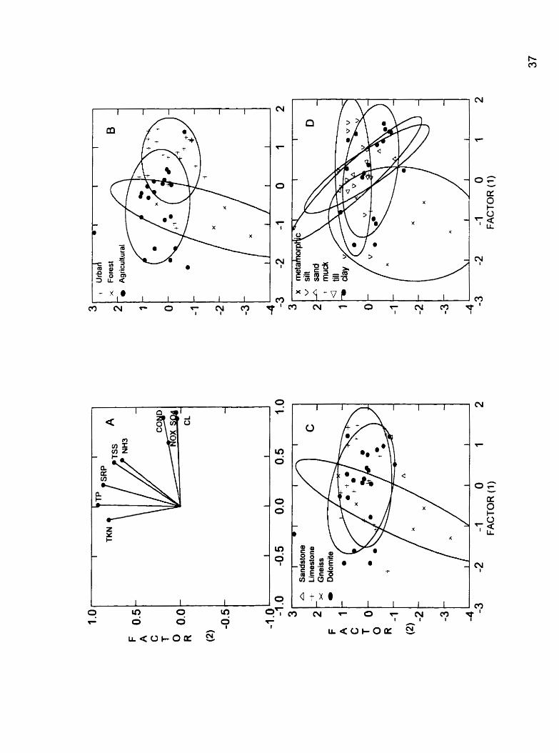
There were two groups of strongly correlated water quality variables (Table 3, Figure 2-

A) that accounted for most of the differences in water quality among sites. The first

group of variables, loading strongly on the first principal component axis, included

chloride, sulfate, nitrate+nitrite and conductivity. The second group, representing

nutrients (soluble reactive phosphorus, total phosphorus, ammonia, total suspended

solids and total Kjeldahl nitrogen) loaded strongly on the second principal cornponent.

Moreover, the PCA on water quality explained more than 75% of the variability in water

quality between sarnpling sites. Forested streams differed frorn urban and rural streams

by having lower nutrient concentrations. Urban sites had typically higher values of CI.

SOs, NOx and conductivity than the rural sites while agricultural sites had equal or

higher values of soluble reactive phosphorus, total phosphorus, ammonia, total

suspended solids and total Kjeldahl nitrogen than the urban sites (Figure 2-8).

Bedrock and surficial geology were poorly correlated with water quality of the sam pling

sites (Figure 2 -C and D) except for gneiss and metamorphic rocks for forested streams

of the Canadian Shield. The overall positions of the ellipses (gneiss and metamorphic)

in Figure 2-C and 2-D were spatially located at an opposite end of both principal

components loadings of water quality (Figure 24).

Taxonornic structure of the invertebrate assemblage.

Over 100 000 individual invertebrates were sampled and sorted into 18 broad

taxonomic groups ranging from order to genus. The most common taxon was

Orthocladiinae accounting for 50% of al1 invertebrates sarnpled. Other important taxa

included Trichoptera, Isopoda, Chironominae, Oligochaeta, Ephemeroptera, Hydra and

Platyhelrninthes with relative densities ranging from 2 to15% (Figure 3). Taxonornic

composition and abundance differed among the urban, rural and forested sites. Urban

streams tended to have abundant Isopoda, Oligochaeta and Orthocladiinae and low

abundance of Plecoptera and Epherneroptera while forested streams had the opposite

tendency (Figure 4 A , B). Meanwhile, abundant Trichoptera, Tanypodinae, Gastropoda,

Platyhelminthes, and Coleoptera characterized rural streams (Figure 4-A. B).

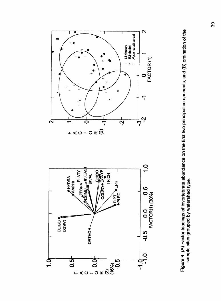
Proportion of Orthocladiinae and relative abundance of sensitive (Plecoptera,

Ephemeroptera) and tolerant taxa (Isopoda and Oligochaeta) were the main axes of

variation in invertebrate assemblages. The first 2 principal components (PCATAXA) of the

analysis on the 16 most common taxa explained 46% of the variance among sites

(Figure 4). The first principal component (PCITAXA) accounted for 30% of the variance

and was positively correlated to the abundance of most invertebrate taxa, but negatively

correlated to Orthocladiinae abundance. In contrast, PCPTnxA (16%) was correlated to

the following ratio: (Isopoda + Oligochaeta) I (Plecoptera + Ephemeroptera).

lnvertebrate comrnunity structure vs. water quality.

Al1 invertebrate assemblage characteristics (PCATAXAl taxa richness, abundance)

responded one way or another to water quality variations (PCAwQ). Assemblage

composition and abundance, described by scores on the first two PC axes, were

significantly related to the principal components of water quality (PCl wQ and PCZwa).

Regression models of the principal components on taxa abundance predicted for 16 to

30% of the variance in abundance (Table 4). Factor 1 (PCITAXA), which represents the

overall abundance of invertebrates, was negatively related to the first principal

cornponent of water quality (PClwQ) and positively related to the second principal

component (PC2 wQ) (Table 4). Factor 2 ( ~ C ~ T A X A ) , proportional to the ratio: lsopoda +

Oligochaeta 1 Ephemeroptera + Plecoptera, was positively related to the first principal

component of water quality (PCl wQ) (Table 4).

Taxa richness increased with increasing nutrients and was significantly related to the

second principal component of water quality (R~=O. 18,~able 5).

Abundance of individual taxa also varied with water quality. Ephemeroptera,

Chironominae, Tanypodinae, D. poiymorpha, and Platyhelmint hes decreased in density

with an increase in ?ClwQ (water conductivity/ions), whereas Simuliidae, Oligochaeta,

Isopoda, and Orthocladiinae increased along the same gradient (Table 6). Abundance

of Chironominae, Gastropoda, Oligochaeta and Platyhelminthes were also positively

related to nutrients (axis 2 of the PCAw~).

Finally, assemblage composition and abundance (described by scores on the fint h o

axes of the PCA on taxa) as well as taxa richness and individual taxa abundance were

not significantly related to the interaction between the two principal components of water

quality (PC1 WQ*PC~WQ).

Size distributions of invertebrates vs. water quality.

The size distribution of the benthic invertebrate assemblage was unimodal with a peak

at around 100pg (4.64mm) (Figure 5). The size spectra for individual taxa were also

unimodal but mean size and the shape of the distribution varied among taxa. (Figure 5).

Body mass was the single best predictor of abundance per size class. Polynomial

models of the size distributions of the different taxa and of the total assemblage

accounted for 10 to 77% of the variance in abundance per size class (Table 7). Water

quality differences among sites accounted for an additional 3 to 23% of the variability.

Responses to water quality differed arnong taxa. Along the conductivity/ionic gradient

(PClwa), Chironominae and Ephemeroptera abundance tended to decrease (Figure 6-

El G) whereas the abundance of Oligochaeta, Orthocladiinae and the total assemblage

tended to be greater in sites with higher conductivity/ions (Figure 6 4 , B. 1, J, M. N)

(Table 7). Abundance of Chironominae, Oligochaeta and of the total assemblage was

higher in sites with high nutrient concentrations (PCZwQ) (Figure 642, F, KI L). The

shape of the size distribution also varied with water quality and responses of taxa

d iffered .

DISCUSSION

Water quality in streams of the Ottawa valley.

Physico-chernical attributes of streams in the Ottawa valley reflected more the land use

than the geology of the watenhed. This suggests that human activities are responsible

for some of the differences in water quality. Indeed, the two main gradients of water

quality (conductivity/ions and nutrient) identified by the K A w Q could be caused by

urbanization and agriculture.

Urban streams are often characterized by high dissolved nitrogen (Lenat and Crawford,

1 994), sulfate (Smith, 1987) and chloride levels (Jones and Clark, 1987). lncreased

sulfate levels can be attributed to the combustion of fossil fuels and to localized

industrial outfalls (Peters, 1984; Hem, 1985; Smith, 1987) while chloride levels. in a

populated northern region, often result from the application of chemical de-icers on

roads, especially NaCl and KCI (Fisher. 1968; Hanes et al, 1970; Peters, 1984; Hem,

1985; Smith, 1987). The application of these chemical agents has been shown to

increase significantly the chloride levels of nearby streams (Peters and Turk, 1981 ;

Scott, 1981 ; McBean and Al-Nassri, 1987; Demers and Sage, 1990; Shanley, 1994).

Rural streams are often characterized by high nutrients and TSS levels (Lystrom, 1978;

Lenat and Crawford, 1994) while forested streams in undeveloped watersheds of the

Ottawa valley are characterized by low nutrient levels (Morin and Nadon, 1991 ;

Bourassa and Morin, 1995).

The geological formations (bedrock and surficial) underlying stream watenheds are

seldom taken into account in biological surveys. Nevertheless, geological formations are

often important non point sources of chemical elements in rivers, for example; Peters

(1 984) found that limestone basins have hig her concentrations of chloride and sulfate

than either sandstone or crystalline basins. The geological formations of Eastern

Ontario and Western Québec are composed of numerous and distinct geological

assemblages including sedimentary rocks (limestone and dolomite) in the southeast

and metamorphic rocks in the northwest. However, the sampling sites located within the

urban reg ion and agricultural areas have sim ilar bed rock and surficial geolog y since

they were subjected to the same events: glaciation by the Wisconsin sheet, inundation

by the Champlain sea and erosion and deposition of early phase of the Ottawa River

(Water and Earth Science, 1981). Therefore, we are unable to strongly link either

principal components of water quality to the geological formations of urban or

agricultural streams.

The geological formation of the forested stream watershed is very different from that of

the other rivers (urban and agricultural). The low nutrients in the soi1 and surface waters

can be attributed to the underlying geology since gneiss rocks and metamorphic rocks

do not contain or easily leach nutrients to the soi1 or water (Hem, 1985, Birkeland and

Larson, 1989). Since the forested basin is not suitable for agricultural practices little

nutrients flow in these rivers.

Problems associated with the correlations between water quality parameters.

The ultimate goal in biornonitoring studies is to show causal relationships between

invertebrate assemblages and water quality, often described as separate entities (CI,

S04, TP, etc). However, the results of this study and of another similar study (Yu et al,

1995) often reveal strong correlations between various water quality parameters. Since

the aquatic invertebrates are exposed to a combination of chernical parameters present

in the water, predictive models of invertebrate characteristics (abundance, taxa

richness) should include the chemical parameters as groups instead of individual

parameters. A principal components analysis (PCA) is an easy and practical way to

group the water quality parameters. In this case, not only did the PCA on water quality

explain over 75% of the variability of water quality between sites, but it also separated

the 9 physico-chemical parameten into only 2 groups. Furthemore, the relationships of

the parameters within a group were easily interpretable. Therefore, due to the numerous

correlations found between the water quality parameters (Figure 244, Table 3) we are

unable to predict if the various invertebrate characteristics (PCATAxn, abundance, taxa

richness and size distributions) are affected solely by an individual parameter or a

combination thereof.

Taxonomic structure of the invertebrate assemblage.

The taxonomic composition of the invertebrate assemblages is similar to that previously

reported in creeks of the Ottawa valley (Bourassa and Morin, 1995). Orthocladiinae

were found over the entire range of sampling sites and they were the dominant taxon,

especially in the most urbanized sites. Orthocladiinae are considered opportunistic and

tolerant of physico-chemical disturbances (Jones and Clark, 1987). They also prefer

rocky substrates (Peckarsky, 1990) like the cobbles and rocks that were sampled.

Abundances of Isopoda, Oligochaeta, and Orthocladiinae were correlated and tended to

be highest in the urbanized sites. It has been previously reported that stressed systems

are usually dominated by few taxa (Resh and Jackson, 1993; Lenat and Crawford,

1994). These taxa contain species that are rather tolerant to a variety of physico-

chemical stresses (Barton and Farmer, 1997; Jones and Clark, 1987).

Agricultural streams had more CO-dominant taxa (Trichoptera, Gastropoda, Coleoptera,

Platyhelminthes, Chironominae and Tanypodinae) than urban or forested streams

probably because of the high nutrients and low physico-chernical stresses associated

with urbanization. The increase in nutrients in these waters could accommodate more

scrapers as well as herbivore invertebrates (Trichoptera, Gastropoda, Coleoptera and

Chironominae).

Gill breathing taxa such as Ephemeroptera and Plecoptera are often absent from highly

impacted sites. Both rural and forested streams had high abundances of Plecoptera and

Ephemeroptera compared to urban streams maybe because of the lower concentrations

of toxic compounds associated with the urban region (CI, S04, and NO,) and low

suspended solids (TSS) levels found in forested streams.

lnvertebrate assemblages reflect the type of watershed sampled (urban, agricultural or

forested) as well as the individual abilities of the invertebrates to withstand physico-

chernical stresses (Figure 4). Along the first principal component (PCIm), Oligochaeta

and lsopoda are clumped together. These two groups dominate urban creeks and are

highly tolerant to a variety of physico-chemical stresses (Jones and Clark, 1987). Again,

along P C I T ~ , Hydra, Simuliidae and Arnphipoda are grouped together and they CO-

dominate urban and agricultural areas. Platyhelminthes, Gastropoda, Chironominae,

Tanypodinae, Bivalvia, Coleoptera and Trichoptera are clumped together along f CZTAXA

and dominate the agricultural streams. These groups contain species that can be either

tolerant or sensitive to pollution. Finally, Diptera, Plecoptera and Ephemeroptera are

grouped together along PCZTAXA and CO-dominate both agricultural and forested

streams. Previous studies suggests that Plecoptera and Ephemeroptera are very

sensitive to physico-chemical stresses (Short et al, 1991 ; Olive et al, 7 992).

lnvertebrate community structure vs. water quality.

Proportion of Orthocladiinae (PCITAXA) increased with an increase in conductivity/ions

(PClwa), and decreased with increasing nutrients (PC2wQ). Previous studies have

found that chloride negatively affects numerous taxa (Olive et al. 1992, Havas and

Hadvokaat, 1995) and the observed pattern suggests that Orthocladiinae are less

sensitive than average to chloride stress. lncreases in nutrients generally translate into

increases in algae and other primary producers, which are at the base of the foodweb of

herbivore invertebrates (Lenat and Crawford , 1 994). Apparently, Orthoclad iinae do not

respond as strongly as other invertebrates to nutrient increase since their relative

abundance declines with eutrophication.

The ratio (PCZTM) of (( tolerant » (Isopoda, Oligochaeta) to (( intolerant » taxa was

positively related to conductivity/ions (PC 1 wo). Pfenet and Gibert (1 994) found that the

total abundance of invertebrates was positively related to conductivity. Since Isopoda,

Orthocladiinae and Oligochaeta dominated the invertebrate assemblages, and since

they respond positively to an increase in conductivity, the results of this study support

the observations of Plenet and Gibert (1 994).

Taxa richness was influenced positively by nutrients (PCZwQ). An increase of nutrients

in streamwater usually translates into increase in food availability and diversity, which in

turn can support a more diverse fauna of invertebrates. Cao et al (1986) also found that

species richness increased with a slight increase in organic pollution.

Densities of sensitive taxa such as Ephemeroptera, Platyhelminthes, Chironominae,

and Tanypodinae were al1 negatively related to conductivity/ions (PClwa). This is partly

in concordance with other studies that have shown different tolerance levels to Sa4, CI

or conductivity by different taxa (Short et al, 1991 ; Olive et al, 1992; Plenet and Gibert,

1994; Havas and Hadvokaat, 1995; Soulsby et al. 1997).

Chironominae, Gastropoda, Oligochaeta and Platyhelminthes were positively related to

nutrients (PC2wQ). Similar increases in abundance with increases in nutrients have

been reported and discussed previously.

Size distributions of the invertebrate assemblage vs. water quality.

Observed size distributions were very similar to previously reported macroinvertebrate

size distributions (Morin and Nadon, 1991, Bourassa and Morin, 1995). Bourassa and

Morin (1995) also found that mass was the single most important predictor of

invertebrate abundance per size class. Water quality accounted for only an additional 3

to 23% of the variability depending on the taxa taken into account.

The size distributions of the total assemblage as well as those of the dominant taxa are

slightly affected by changes in water quality (PCl Wa and PCZwQ) (Table 7). The density

per size class of the total assemblage as well as Oligochaeta and Orthocladiinae

increases with an increase in conductivity/ions (PCIWQ) (Figure 6) (Table 7). A high

tolerance to urbanization as been previously reported for these groups (Jones and

Clark, 1987; Cao et al, 1986; Mulliss et al, 1996). The density per size class of the total

assemblage as well as Chironorninae and Oligochaeta increases with an increase in

nutrients (PC2wQ) (Figure 6). Some species of Oligochaeta have been known to thrive

under high organic pollution levels (Peckarsky , 1990). In addition, the increase in

nutrients in these waters could accommodate more scrapers (Chironominae). The

density per size classes of Epherneroptera decreases with an increase in

conductivity/ions (PCl wQ). A low tolerance to chloride/sulfate as been previously

reported for Ephemeroptera (Short et al, 1991 ; Soulsby et al, 1997).

Few studies have reported the size distributions of dominant taxa of lotic invertebrates

probably because of the tirne-constraints associated with first identifying the

invertebrates and then measuring their mass. However, as the results of this study

show, the additional time required to measure the size distribution of individual taxa is

warranted. The responses of individual taxa to changes in water quality differed from

one another and the size distribution of the total assemblage shifted as the distribution

of its dominant taxa. In this case, the size distribution of the total population reflects

rnainly that of Orthocladiinae (which comprise about 50% of the total population) and

Trichoptera. 1 he size distribution of the total assemblage is very similar to the

distribution of Orthocladiinae, especially for the invertebrates measuring between 3 and

10rnm (Figure 5). Furthenore, the size distribution of the total assemblage is sirnilar to

the distribution of Trichoptera for animals measuring between 1 and 2.6 mm as well as

those from 14 to 46mm. Therefore, taxon-based size distributions enabled us to

evaluate more precisely the effects of water quality on stream invertebrates.

Importance of the taxonornic resolution in the family Chironomidae.

In most biornonitoring studies, rnidges are only identified at the family level of

Chironomidae instead of classifying them into their respective sub-families:

Orthocladiinae, Chironominae, Tanypodinae, etc (Thorne and Williams, 1997; Lenat and

Crawford, 1994). Because the sub-families have very different responses to water

quality, lumping al1 rnidges together is not appropriate. Orthocladiinae seern to be very

tolerant and thrive despite pollutants (chloride, sulfate) while Chironominae and

Tanypodinae seem much less tolerant. Recent studies have begun to debate the need

for higher taxonornic resolution in the Chironomidae family (Resh and Jackson, 1993).

The results reported here advocate in favor for identification at least at the sub family

level.

Quality of predictions and other factors affecting invertebrate abundance.

The residual variance can be used as a metric of the precision of predictive models and

the stridy by Morin (1 997) provides typical ranges for various estimates of invertebrate

abundance (both daily-mean and size spectra models). Overall, the precision of the

models predicting abundance of invertebrates in this study is generally weak. The

precision of the models of invertebrate abundance in this study is much worse than that

of typical models and measurements reported by Morin (1 997). However, precision of

the size spectra models was similar to those reported by Morin (1 997). Therefore, the

size distribution models could be qualified as precise.

Another way to assess the quality of predictions from predictive models is to compare

the magnitude of prediction errors (RMS) to that of measurement errors (pure error). If

the RMS approaches pure error, then al1 of the variability among sites has been

accounted for. However. since RMS values were always much larger than the estimates

of pure error (Tables 5-7), a large proportion of the variability among sites rernained

unexplained by the regression models. Therefore, other factors are affecting

significantly the Stream invertebrate assemblages in the Ottawa valley.

Heavy metals in the water (Timmermans et al, 1989; Bervoets et al, 1994, Schumacher

et al. 1993), heavy metals in sediments (Beauvais 1995; Pinochet et al, 1995;

Schumacher et al. 1995). pesticides (Cheevaparanapiwat and Menasveta, 1981 ; Elder

and Mattraw, 1984), PCB (Cheevaparanapiwat and Menasveta, 1981; Elder and

Mattraw, l984), insecticides (Greichus et al., 1977) and other unmeasured toxic

chernicals may well affect invertebrates. The single or synergetic effects of these

parameters rnay account for compositional differences among sites that are not related

to nutrients or conductivity/ions. However, inorganic and organic pollutants in stream

waters from the Ottawa Valley are generally at trace levels (RMOCA,B, 1993), and it

seems unlikely that the unexplained variability in invertebrate abundance among sites

could be explained by pollutants.

It seems more likely that stochastic factors, differences in ph ysical factors (poollriffle

ratios, moss cover, etc) or in food availability (detritus, diatoms), or differences in fish

predation pressure among sites could account for the variability unexplained by the

regression rnodels.

Prioritizing interventions.

The majority of stream invertebrate characteristics (abundance, taxa richness, size

distributions) were negatively related to the first principal component of water quality

(composed of NO,, CI, S04 and conductivity). This leads us to hypothesize that a

decrease of the first principal component of water quality would be beneficial to the

invertebrate assemblage of this region. However, since there are strong correlations

between the three physico-chernical variables comprising the first principal component

of water quality. we are unable to correctly identify the main stressor. Therefore, we

suggest that the abatement of al1 three physico-chernical parameters (chloride, sulfate

and nitrate+nitrite) should be a priority of the different levels of municipal. regional.

provincial and federal agencies present in the Ottawa valley.

CONCLUSION

A principal components analysis on the water quality parameters revealed that two

groups of correlated variables explained most of the variability among sites. Both

principal components were strongly linked to land usage: PClwQ represented a kind of

urbanization gradient while PC2wQ represented nutrients. C haracteristics of the stream

macroinvertebrate assemblages of the Ottawa valley (abundance, taxa richness and

size distribution) were shown to be related to water quality. Overall, both principal

ccrnponents of water quality were good predictors of invertebrate characteristics

(abundance, taxa richness or size distribution). Given the origin of the ions included in

the principal components, it appears that human activities are affecting the distribution

of invertebrates in streams of the Ottawa valley.

FIGURES

Figure 2. (A) Factor loadings of the water quality parameters on the first two principal components, and (B) ordination of the sampted sites grouped by watershed type, bedrock geology (C), and surficial geology (D). Ellipses are the 68% confidence ellipses.

a - x a n A l A 1 4 4 v T A

k < o t O K C?

Chironominae

1

Total

1

b

Ephemeroptera

I

Oligochaeta

* Tanypodinae I

Trichoptera

t

Figure 5. Size distributions of the dominant taxa and of the total assemblage of stearn invertebrates. Mean log (density+lO) with SE (n=8).

Figure 6. Predicted size distributions of stream invertebrates as a function of water quality. Lines are the densities predicted by the models of Table 7 at low, medium and high values of PClwQ (or PCSwQ) while PCZwQ (or PClwo) was kept at a mean value. Low values of PClwQ are represented by sites with low concentrations of chloride, nitrate and nitrite, conductivity and sulfate while low values of PCZwQ are represented by sites with low concentrations of total suspended solids, total phosphorus, soluble reactive phospharus, total Kjeldahl nitrogen and ammonia. High values of PClwa are represented by sites with high concentrations of chloride, nitrate and nitrite, conductivity and sulfate white high values of PCZwQ are represented by sites with high concentrations of total suspended solids, total phosphorus, soluble reactive phosphorus, total Kjeldahl nitrogen and ammonia.

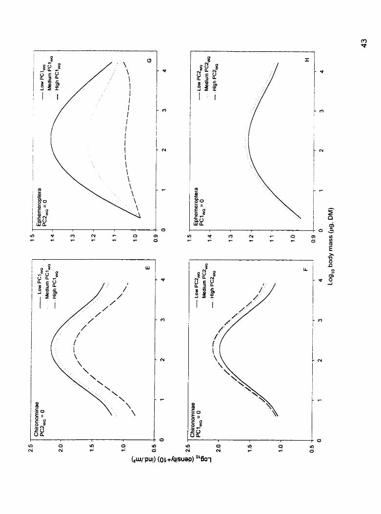
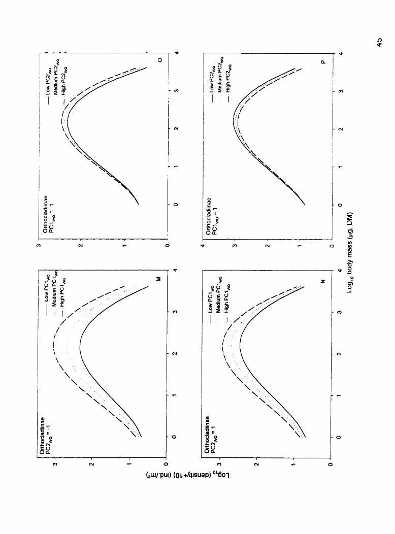
Table 1. Location and characteristics of the sampling sites. -- -

River Site # ~afitude Longitude Landscape Geology (generalized bedrock) Geology (surficial materials) Bear Brook

Bilberry Ck.

Black Rapids Carp River

Castor Creek

Chelsea Ck.

Coady Creek Graham Ck.

Green's Ck.

Hunt Club Jock River

Lemay Creek Lenard Creek Mud Creek Outaouais R. Pinecrest Ck.

BEAO1 BEA02 BI LO 1 BI L02 BLAOI CARO1 CAR02 CAR03 CAR04 CAS01 CAS02 CAS03 CAS04 CHE01 CHE02 CHE03 CHE04 COD01 GRAOl GRA02 GREOt GRE03 GREM HUNOI JOCO1 JOC08 LEM01 LENOI MUDO1 on02 PIN01

75O18W 75OO5'W 75O32W 75"30tW 7504ZfW 76" 1 2'W 75"55'W 76" 1 O'W 75"54'W 75"23'W 75'32'W 75"21tW 75"30W 75O44'W 75"47'W 75"49'W 75"50'W 76" 12W 75"4B'W 75O47'W 75O35W 75O36W 75O35'W 75"4 1 'W 75O42'W 75"58'W 75"45'W 75"30'W 75"42'W 75"45'W 75"47'W

Agricultural Agricultural Urban Urban Urban Agricultural Agricultural Agricultural Agricultural Agricultural Agricultural Agricultural Agricultural Forest Forest Forest Forest Agricultural Urban Urban Urban Urban Agricultural Urban Agricultura t Agricultural Urban Agricultural Agricultural Agricul tural Urban

Shale (thin dotornite)// Black shale Shale (thin dolomite)// Black shale Limestonell Shale and sandstone Limestone Dolomite Dolomite and Iimestone Limestone (some sandstone) Dolomite and Iimestone Limestone (some sandstone) Dolomite and sandstone Dolomite and sandstone Dolomite and sandstone Grey shale and dolomite Gneiss Paragneiss Gneiss Gneiss Limestone and dolomite Dolomite and limestone Dolomite and limestone Shale and lirnestone Shale and limestone Shale and lirnestone Limestone Dolomite and limestone// Quaternary Dolomite and limestone Unknown (Quaternary) Limestone Dolomite Limestone , sandstone Lirnestone

Yellow-find sand, silt, clay, till Sand, silt, clay Silt and silty clay Blue-grey clay, silt Blue-grey clay, silt and silty clay Clay, silt and intrusive, metamorphic rocks Till, clay and sand Clay, silt and intrusive, metamorphic rocks Muck and peat, sand, grave1 Till, clay, silt, and sand Till, clay, silt, and sand Till, clay, silt, and sand Till, clay, silt, and sand lntrusive and metamorphic rocks lntrusive and metamorphic rocks lntrusive and metamorphic rocks Intrusive and rnetamorphic rocks Blue-grey clay, silt and silty clay Blue-grey clay, silt and silty clay Blue-grey clay, silt and silty clay Blue-grey clay, silt and silty clay, muck and peat Blue-grey clay, silt and silty clay Blue-grey clay, silt and silty clay, rnuck and peat Yellow-fine sand, till and clay Muck and peat, clay and silt Blue-grey clay, silt and silty clay Silt and silty clay Silt and silty clay Blue-grey clay, silt and silty clay Silt and silty clay Till, silt and sand

PIN02 45"2 1'N 75"46'W Urban Limestone Silt and silty clay

- - --

River Site # Latitude Longitude Landscape Geology (generalized bedrock) Geology (surficial materiak) - Rideau River RlDOl 45O25'N 75"401W Urban Lirnestone and shale Clay and silt

RID04 45O22'N 75O4 1'W Urban Limestone Clay and silt RIDO7 45O14'N 75O40W Agricultural Dolomite Blue-grey clay, silt and silty clay

Sawmill Ck SAWOl 45O23'N 7!i040'W Urban Black shale and dolomite Silt and silty clay SAW02 45O20'N 75'37W Urban Grey shale Yellow-fine sand

South Nation SOU01 45'32'N 74O59W Agricultural Limestone, shale Silt, clay, sands and silty clay SOU02 45'19'N 75'05W Agricultural Limestone and shale Silt, clay , sands and silty clay SOU03 45'1 3'N 75O09'W Agricultural Limestone and shale Silt, sands and silty clay SOU04 44O59'N 75O27W Agricultural Dolomite and sandstone Silt, sands and silty clay SOU05 44"50'N 75O32'W Agricultural Dolomite and sandstone Silt, sands and silty clay

Stillwater Ck. STlOl 45O20'N 75O49'W Urban Dolomite and limestone Silt, blue-grey clay and silty clay Watt's Creek WATOl 45'20'N 75O53'W Urban Dolomite and limestone Silt and silty clay

WAT02 45O19'N 75O55'W Urban Dolomite and limestone Blue-grey clay, silt and silty clay WAT03 45O20'N 75O54W Urban Sandstoneii Dolomite and limestone Blue-grey clay, silt and silty clay WAT04 45O18'N 75O54'W Urban Sandstoneii Dolomite and limestone Blue-grey clay, silt and silty clay

Table 2. Physico-chernical parameters of the rocks sampled and the sampling sites. With the exception of five sampling sites, the conceiitration of chloride, conductivity, ammonia, nitate+nitrite, sulfate, soluble reactive phosphorus, total Kjeldhal nitrogen, total phosphorus and total suspended solids are annual means. Legend: * - (Denotes sites with a single observation), Type - (Type of watershed), A - (Surface area of the rock), D - (Depth where the rock was collected), VI - (Water velocity at maximum water depth), V2 - (Water velocity at 60% of the water depth), Peri - (Periphyton) (mg chlalrn2), CI - (Chloride), Con - (Conductivity), NH3 - (Ammonia), NOx - (Nitrite and nitrate), S04 - (Sulfate), SRP - (Soluble reactive phosphorus), TC - (Water temperature). TKN - (Total Kjeldahl ritrogen), TP - (Total phosphorus), TSS (Total suspended solids).

Station Type A D V1 V2 Peri Cl Con NH3 NO, pH SO, SRP TC TKN TP TSS Cm2 cm mls mls mglL uSlcm mg/L mg/L mglL mg/L "C mglL mg/L mg/&

BEAOI Agricultural 135.5 12.4 1.93 1.08 32.4 93 690 0.063 0.35 8.1 47 0.04 13 0.78 0.067 10.4 BEA02 Agriculturat 148 6.25 0.59 0.59 34.1 81 579 0.033 0.378 8.1 24 O 17 0.84 0.111 34 BILOI Urban 113.9 9.88 0.85 0.81 60.9 317 1544 0.117 1.091 8.2 86 0.06 15 0.6 0.087 33.3 BIL02 Urban 98.01 6.88 0.68 0.68 49 270 1489 0.028 0.87 7.7 93 0.05 12 0.35 0.052 2.3 BLAOI Urban 135.2 8.75 0.96 0.79 27.4 92 719 0.108 1.734 7.9 22 0.06 10 0.61 0.085 12.9 CARO1 Agricultural 123.8 11.4 0.96 0.78 23.9 91 666 0.0760.307 8.3 29 0.01 13 0.67 0.052 12.8 CAR02 Urban 132.3 6.25 0.55 0.55 118 54 707 0.066 0.178 7.8 73 0.01 9.3 0.82 0.041 6.76 CAR03 Agricultural 172.3 17.8 0.6 0.45 28.1 107 745 0.07 0.297 8.1 34 0.02 15 0.69 0.05 7.5 CAR04 Urban 120.7 8.63 0.93 0.93 34.2 113 806 0.055 0.03 7.3 63 0.02 16 0.56 0.046 11.2 CAS01 Agricultural 95.73 7.25 1.18 1.18 76.8 28 552 0.043 0.495 8.2 42 0.05 17 0.64 0.086 21.6 CAS02 Agricultural 108.7 15 1.01 0.73 52.6 27 531 0,039 0.12 8.1 42 0.26 14 1.44 1.7 18.6 CAS03 Agricultural 127.6 12.3 0.45 0.4 33.7 51 668 0.024 0.237 8.5 91 0.01 17 0.73 0.049 9.48 CASW Agricultural 130.1 8.88 1.35 1.35 28 69 959 0.045 0.094 8.2 137 0.02 21 0.62 0.044 17.3 CHEOI* Forest 124.4 13.5 1.1 0.96 11.4 57 444 0.034 0.745 7.7 16 0.05 14 0.36 0.076 37 CHE02* Forest 291 14.1 0.9 0.76 8.95 59 398 0.004 0.149 8.1 17 O 12 0.28 0.011 1.5 CHE03' Forest 188.8 15.5 1.03 0.99 5.34 40 317 0.007 0.078 8 10 O 13 0.36 0.015 1.6 CHE04' Forest 117 6.13 0.94 0.94 5.19 13 199 0.005 0.16 8 7.4 O 70 0.12 0.005 0.4 COD01 Agricultural 148.2 9.88 1.33 1.26 37.9 35 518 0.05 0.215 8 12 0.07 13 0.67 0.095 16.1 GRAOI Urban 148.5 17.9 0.85 0.7 74.3 208 1137 0*038 1.181 8.2 74 0.01 12 0.39 0.028 7.89 GRA02 Urban 131.4 13.5 0.49 0.43 18.9 117 816 0.037 1.47 8 63 0.02 6.3 0.36 0.045 21.1 GREO1 Urban 11'?.6 11.3 0,94 0.93 38.9 300 1380 0.098 0.285 8 112 0.03 11 0.74 0.067 18.3 GRE03 Urban 137.2 9 0.81 0.75 16.6 220 1$27 0.23 0.33 7.2 85 0.03 14 0.82 0.06 24 GRE04 Agricultural 124.1 14.4 1.6 1.23 49.5 154 1320 0.135 0.27 7.7 220 0.01 16 0.44 0.022 8.4 HUNOl Urban 251 9.13 0.99 0.93 31.9 139 882 0.062 0.474 8.1 66 0.01 13 0.53 0.033 6.36

Station Type A D V I V2 Peri CI Con NH3 NO, pH S04 SRP TC TKN TP TSS Cm2 cm mls mls mglL uS/cm mg/L mc$L mglL mglL OC mglL mg/L mg/L

JOCO1 Agricultural 135.4 16 JOCO8 tEMOlm LENO1 MUDOl OTT02 PIN01 PIN02 RlDOl RIDO4 RI007 SAWOS SAWO2 SOU01 SOU02 SOU03 SOU04 sou05 STIO1 WATOI WAT02 WATO3 WATW

Agricultural Urban Agricultural Agricultural Agricultural Urban Urban Urban Urban Agricultural Urban Urban Agricultural Agricultural Agricultural Agricultural Agricultural Urban Urban Urban Urban Urban

Table 3. Correlation coefficients (p values) between water quality variables. Legend: Peri - (Periphyton) (mg chla/m2), CI - Loglo (Chloride) (mglL), Conduct - Loglo (Conductivity) (pslcm), NH3 - Loglo (Ammonia) (mgll), NOx - Logto (Nitrite and nitrate) (mglL), S04 - Loglo (Sulfate) (rnglL), SRP - Loglo (Soluble reactive phosphorus) (mglL), TKN - Loglo (Total Kjeldahl nitrogen) (rnglL), TP - Loglo (Total phosphorus) (mglL), TSS Logio (Total suspended solids) (mglL).

Peri

CI

Conduct

NH3

NO,

so4

SRP

TKN

TP

TSS

Peri CI Conduct NH3 NO, so4 SRP TKN TP TSS

1 .O00 (0.0)

0.355 (0.521)

0.400 (O. 193)

0.551 (0.002)

0.541 (0.003)

0.462 (0.039)

0.665 (~0.001)

Table 4. Multiple regression models of the principal components on taxa as a function of the principal components of water quality. Legend: PClwQ - (chloride, sulfate, conductivity and nitrate+nitrite), PCPwQ - (total suspended solids, total phosphorus, soluble reactive phosphorus, total Kjeldahl nitrogen, ammonia), SE - (standard error), p - (p values), n - (number of observations), R2 - (proportion of the variance in the data explained by the models), RMS - (Residual mean square).

Dependent Effect Coefficient SE P n R2 RMS Factor 1 Constant 0.000 O. 125 1.000 47 0.301 0.731

Factor 2 Constant 0.000 0.135 1.000 47 O. 156 0.862 pclwa 0.395 O. 137 0.006

Table 7. Multiple regression models predicting the density per size class of the total assemblage and of the dominant taxa. Legend: M-Log10 (dry mass) (pg), P C ~ W Q - (chloride, sulfate, conductivity, nitrate+nitrite), PCZwQ - (soluble reactive phosphorus, total phosphorus, total Kjeldahl nitrogen, total suspended solids, ammonia), Coeff. - (Coefficient), SE - (standard Error), p - (p value), R2 - (proportion of the variance in the data explained by the models), RMS - (Residual mean square), PE - (Pure error).

Taxa Effect Coeff. SE P R2 RMS PE Total Constant

M M2 M" hl4

Constant M M2 Ma M~ PC1 wa PC2wa M*PC 1 M*PCl wa*PC2wa M2 'PClwQ PC2wa*PC2wa

C hironominae Constant M M2 M3 M~

Constant M M2 MJ M' ~ C ~ W Q M'PC2wa PC 1 wa'PCl wa PCZwa'PC2wa

Ephemeroptera Constant M M2

Constant M Ma M~ PCl wa M*PC7wQ M2 'PClwa

Taxa Effect Coeff. SE P R2 RMS PE lsopoda Constant O. 794 0.047 0.000 0.105 0.050 0.009

Constant M M3 M~ MaPClWQ M' *PClwa PC1 wa*PCl wa

Oligochaeta Constant M MS M~

Constant M M3 M4

Orthocladiinae Constant M M2 M3 M~

Constant M M2 M3 M~ PClwa M'PC 1 wQ Mz 'PCI wa M'PCl wa'PC2wa

Taxa Effec t Coeff. SE P R2 RMS PE Tanypodinae Constant 0.702 0.054 0.000 0.195 0.041 0.01 1

M 0.445 0.059 0.000 M5 -0.060 0.012 0.000 hl4 0.009 0.002 0.000

Trichoptera Constant M MZ M~

Constant 1.013 0.042 0.000 0.333 0.136 0.025 M 0.70 1 0.059 0.000 MZ -0.181 0.020 0.000 M~ 0.002 0.000 0.000 PC~WQ -0.094 0.014 0.000 M*PCZwa 0.051 0.01 7 0.003 M'PCl wQ'PC2wQ -0.016 0.005 0.001 M2 'PC2wQ -0.010 0.004 0.01 9 PC 1 wa'PCl wa -0.089 0.01 3 0.000

APPENDICES

Appendix 1. Taxon-specific intercept (a) and exponent (b) of the formula M = ~ L ~ , where M is the body rnass (pg, DM) of a specific group of invertebrate and L is the body length (central axis) (in mm)

- - -- -

Taxon a b Source Chironominae 5.097 2.32 Smock. 1980 Ephemeroptera 6.5979 2.88 smock; 1980 lsopoda 9.602 2.728 Adcock, 1979 Oligochaeta 1 2 Lindengaard et al. 1994 Orthoclad iinae 5.097 2.32 Smock, 1980 Tanypodinae 3.8 2.41 Smock, 1980 Trichoptera 1.928 3.12 Smock, 1980 Total Population 1 3 Morin and Nadon, 1991

Appendix 2. Mean Loglo (density+lO) for each taxon at each sampling site. Legend: Station - (sampling station), EPH - (Ephemeroptera), PLEC - (Plecoptera), TRICH - (Trichoptera), COL - (Coleoptera), CHlR - (Chironominae), ORTH - (Orthocladiinae), TANY - (Tanypodinae), SlMU - (Simuliidae), DlPT - (Diptera), GAST - (Gastropoda), ZEBR - (Zebra mussels), BlVA - (Bivalvia), AMPH - (Amphipoda), ISO - (Isopoda), NEM - (Nematoda), OLlG - (Oligochaeta), PLAT - (Platyhelminthes), HYDR - (Hydra), XYZ - (unknown).

Station €PH PLEC TRICH COL CHlR ORTH TANY SlMU DlPT GAST ZEBR BlVA AMPH ISO NEM OLlG PLAT HYDR XYZ

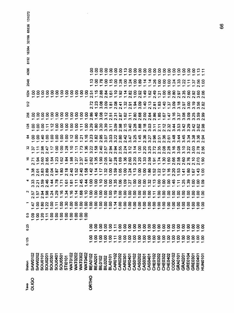
Appendix 3. Average loglo (density + I O ) per size classes (mass, pg) by sampling stations (47) and by taxa (8).

Mass 0.125 0.25 0.5 1 2 4 8 16 32 ô4 128 256 512 1024 2048 4096 8192 16384 32768 65536 131072 Taxa Station CHlRO BEAOl02 1.00 1.00 1.00 1.52 2.69 2.98 3.08 2.84 2.67 2.76 2.27 1.28 1.00

BEA0201 1.00 1.00 1.00 7.22 1.50 1.70 1.77 1.68 1.48 1.21 1.21 1.06 1.00 ML0 102 1.00 1.00 1.00 1.00 1.00 1.00 1.12 1.12 1.29 1.29 1.13 1.00 1.00 SILO202 1.00 1.00 1.00 1.00 1.27 1.57 1.92 1.81 1.88 2.20 1.31 1.14 1.00 BtA0101 1.00 1.00 1.13 1.84 2.02 2.89 2.80 2.71 2.71 2.77 2.71 1.15 1.00 CAR01 02 1.00 1.00 1.11 1.41 2.33 2.80 2.98 2.52 2.53 2.29 1.25 1.00 1.00 CAR0202 1.00 1-00 1.16 1.30 1.59 1.74 1.92 1.75 1.28 1.14 1.00 1.00 1.00 CAR0301 1.00 1.09 1.24 1.69 2.69 3.09 3.09 2.77 2.52 2.07 1.44 1.23 1.00 CAR0401 1.00 1.00 1.00 1.11 1.66 2.21 2.27 1.58 2.08 1.96 1.22 1.00 1.00 CAS01 02 1.00 1.00 1.00 1.13 1.53 2.28 2.65 2.08 1.51 1-12 1.00 1.00 1.00 CAS0202 1.00 1.00 1.00 1.00 1.00 1.16 1.43 2.50 2.66 2.85 2.24 1.10 1.00 CAS0301 1.00 1.00 1.13 1.57 1.49 2.20 2.10 2.06 1.94 2.09 1.92 1.32 1.00 CAS0401 1.00 1.00 1.12 1.43 2.45 2.67 2.67 2.53 1.87 2.14 1.78 1.00 1.00 CHE0102 1.00 1.00 1.13 1.13 1.22 1.72 2.06 1.62 1.i3 1.12 1.00 1.00 1.00 CHE0202 1.00 1.00 1.00 1.03 1.42 1.52 1.18 1.26 1.03 1.19 1.15 1.00 1.00 CHE0302 1.00 1.08 1.30 1.96 2.40 2.69 2.33 1.89 1.61 1.23 1.09 1.00 1.00 CHE0402 1.00 1.00 1.00 1.00 1-00 1.00 1.00 1.00 1.00 1.00 1.00 1.00 1.00 COD01 02 1.00 1.00 1-00 1.00 1.52 1.80 2.14 2.10 1.56 1.83 1.59 1.00 1.00 GRAOlOl 1.00 1.00 1.00 1.00 1.00 1-00 1.00 1.00 1.00 1.00 1.00 1.00 1.00 GRA0201 7.00 1.00 1.00 1.28 1.47 1.38 1.76 1.99 1.68 1.68 1.10 1.00 1.00 GRE0104 1.00 1.00 1.00 1.00 1.00 1.15 1.25 1.34 1.00 1.15 1.15 1.00 1.00 GRE0301 1.00 1.00 1.00 1.12 1.20 t.36 1.39 1.26 1.25 1.14 1.25 1.00 1.00 GRE0401 1.00 1.00 1.00 1.00 1-00 1.13 1.22 1.26 1.46 1.13 1.00 1.00 1.00 HUN0301 1.00 1.00 1.00 1.00 1.00 1.00 1.18 1.09 1.17 1.00 1.00 1.00 1.00 JOC0107 1.00 1.00 1.11 1.49 2.19 2.74 2.76 2.42 2.06 2.11 1.67 1.12 1.00 30CO804 1.00 1.00 1.00 1.39 1.99 2.09 1.89 1.79 2.06 1.60 1.24 1.00 1.00 LEM0102 1.00 1.00 1-00 1.00 1.00 1.12 1.25 1.10 1.00 1.00 1.00 1.00 1.00 LENO102 1.00 1.00 1.00 1.00 1.00 1.16 1.16 1.43 1.13 1.00 1.00 1.13 1.00 MUDO101 1.00 1.00 1.32 2.04 3.04 2.99 3.02 2.84 2.40 2.42 2.09 1.11 1.00 OTT0207 1.00 1.00 1.13 1.13 1.34 1.48 1.45 1.32 7.00 1.00 1.00 1.00 1.00 PIN01 02 1.00 1-00 1.00 1.00 1.00 1.00 1.00 1-00 1-00 1.00 1.00 1.00 1.00 PIN0202 1.00 1.00 1.00 1.00 1.00 1.00 1.00 1.00 1.11 1.00 1.00 1.00 1.00

Taxa Station

CHlRO RI00107 RD0407 RI00707 SAW0102 SAW0202 SOU0101 SOU0201 SOU0301 S0U0401 SOU0501 STlO't O1 WATO 1 02 WAT0202 WAT0302 WATû402

€PH BEA0102 BEA0201 BlL0102 BIL0202 BLAOlOl CARO1 02 CAR0202 CAR0301 CAR0401 CAS01 02 CAS0202 CAS0301 CAS040 1 CHE0102 CHE0202 CHE0302 CHE0402 COD0102 GRAO101 GRA020 1 GRE0104

Taxa Station

ISo WATO402 OLlGO BEA0102

BEA0201 BIL0102 BIL0202 BLA0101 CAR01 02 CAR0202 CAR0301 CAR0401 CAS01 02 CAS0202 CAS0301 CAS0401 CHE0102 CHE0202 CHE0302 CHE0402 COD01 02 GRAOl01 GRA0201 GRE0104 GRE0301 GRE0401 HUNO101 JOC0107 JOC0804 LEM0102 LENO102 MUDO101 On0207 PIN0102 PIN0202 RIDO107 RID0407 RID0707

Taxa Station

ORTHO JOCOlO7 JOC0804 LEM0102 LENOl O2 MUDO101 OIT0207 PIN0102 PIN0202 RID0107 RIDO407 RID0707 SAW0102 SAW0202 S0U0101 S0U0201 SOU0301 SOU0401 SOU0501 STIOS03 WATO102 WAT0202 WAT0302 WAT0402

TANY BEA0102 BEA0201 BILO102 BIL0202 BIAO1 01 CARO3 02 CAR0202 CAR0301 CAR0401 CAS01 02 CAS0202 CAS0301 CAS0401

Taxa Station

TRICH MUDO101 OTT0207 PIN0102 PIN0202 RIO0107 RI00407 RID0707 SAW0102 SAWO202 SOU0101 SOU0201 SOU0301 SOU0401 SOU0501 ST10101 WATO102 WATO202 WAT0302 WAT0402

REFERENCE

Adcock J.A. (1979). Energetics of a population of the lsopod Asellus aqoaticus: Life history and production. Fresh water Siology , 9, 343-355.

Barton DR., & Farmer M.E.D. (1997). The effects of conservation tillage practices on benthic invertebrate communities in headwater streams in southwestern Ontario, Canada. Environmental Pollution , 96, 207-21 5.

Beauvais G.J. (1995). Cadmium and mercury in sediment and burrowing mayfly nymphs (Hexagenia) in the upper Mississippi River. Archives of Environmental Contamination and Toxicology, 28, 1 78-1 83.

Bervoets L., Int Panis L., 8 Verheyen R. (1994). Trace metal levels in water, sediments and Chironomus gr. thumni, from different water courses in Flanders (Belgium). Chemosphere, 29, 1 591 -1 601.

Birkeland P.W., 8 Larson E.E. (1989). Putnam's geology. Oxford: Oxford University Press.

Bourassa N., & Morin A. (1 995). Relationships between size structure of invertebrate assemblages and trophy and substrate composition in streams. Journal of the North American Benthological Society, 74, 393403.

Cao Y., Bark A.W., 8 Williams P. (1986). Measuring the response of macroinvertebrate communities to water pollution: a cornparison of multivariate approaches, biotic and diversity indices. Hydrobiologia, 34 1, 1-1 9.

Cheevaparanapiwat V., & Menasveta P. (1981). Heavy metals, organochlorine pesticides and PCB's in green mussels, mullets and sediments of river mouths in Thailand. Manne Pollution Bulletin, 12, 1 9-25.

Cosser P.R. (1 988). Macroinvertebrate cornmunity structure and chemistry of an organically polluted creek in South-East Queensland. Australian Journal of Marine and Freshwater Research, 39, 67 1-683.

Demers C.L., & Sage R.W. (1990). Effects of road deicing salt on chloride levels in four Adirondack streams. Water, Air and Soi1 Pollution, 49, 369-373.

DeWalt RE., & Olive J.H. (1988). Effects of eroding glacial silts on the benthic insects of silver Creek, Portage County , O hio. Ohio Journal of Science, 88, 1 54-1 59.

Doeg T.J., & Koehn J.D. (1 994). Effects of draining and desilting a small weir on downstream fish and macroinvertebrates. Regulated Rivers Research and Management 9,263-275.

Elder J.F., 8 Mattraw H.C. (1984). Accumulation of trace elements, pesticides, and polychlorinated biphenyls in sediments and the clam Corbicula manilensis of the Apalachicola. Archives of Environmental Contamination and Toxicology, 13, 469

Fisher D.W. (1 968). Atmospheric contributions to water quality of steams in the Hubbard Brook experimental Forest: New Hampshire. Water Resources Research, 4, 1115-1126.

Greichus Y.A., Greichus A., Amman B.D., Call D.J., Hamman D.C.D.. 8 Pott R.M. (1 977). Insecticides, polychlorinated biphenyls and metals in African lake ecosystems. 1. Hartbeespoort dam, Transvaal and Voelvlei dam, Cape province, Repu blic of South Africa. Archives of Environmentai Contamination and Toxicology, 6, 383

Hanes R.E., Zelazny L.W., & Blaser R.E. (1970). Effects of deicing salts on water qua1 ity and biota . National Cooperative High way Research Program Report, 9 1, 1-70,

Havas M., & Hadvokaat E. (1995). Can sodium regulation be used to predict the relative acid-sensitivity of various life-stages and different species of aquatic fauna? Water, Air and Soi1 Pollution, 85, 865-870.

Hem J.D. (1985). Study and interpretation of chernical characteristics of natural water. USGS- Water Supply Paper, 2254, 1 -202.

Jones R.C, & Clark C.C. (1 987). Impact of watershed urbanization on stream insect communities. Water Resources Bulletin, 23, 1047-1 055.

Lenat D.R., & Crawford J.K. (1994). Effects of land use on water quality and aquatic biota of three North Carolina Piedmont streams. Hydrobiologia, 294, 1 85- 1 99.

Lindengaard C., Hamburger K., & Dall P.C. (1994). Population dynamics and energy budget of Manonina southemi (Cernosvitov) (Enchytraeidae, Oligochaeta) in the shallow littoral of Lake Esrom, Denmark. Hydrobiologia, 278, 291-301.

Lystrom D.J. (1978). Regional analysis of the effects of land use on stream water quality, methodology, and application in the Susquehanna River basin, Pennsylvania and New York. USGS-Water-Resources Investigation., 78, 1-60.

Marchant R., Hirst A., Norris R.H., Butcher R., Metzeling L., &Tiller D. (1 997). Classification and prediction of rnacroinvertebrate assemblages from running waters in Victoria, Australia. Journal of the North Amencan Benthologicai Society, 16, 664-681 .

McBean E., & AI-Nassri S. (1 987). Migration pattern of deicing salts from roads. Journal of Environmental Management, 25, 23 1 -238.

Morin A., 8 Nadon D. (1991). Size distributions of epilithic lotic invertebrates and implications for community metabolism. Journal of the No& American Benthological Society, IO, 300-308.

Morin A.. Rodriguez M.A., & Nadon D. (1995). Temporal and environmental variation in the biomass spectrum of benthic invertebrates in streams: an application of thin- plate splines and relative warp analysis. Canadian Journal of Fishenes and Aquatic Science, 52, 1 88 1 -1 892.

Morin A. (1997). Empirical models predicting population abundance and productivity in lot ic systerns. Joumal of the North Amencan Benthological Society, 7 6, 3 1 9-3 37.

Mulliss R.M., Revitt DM., & Shutes R.B.E. (1996). A statistical approach for the assessrnent of the toxic influence on Gammarus pulex (Amphipoda) and Aselus (Isopoda) exposed to urban aquatic discharge. Water Research, 30, 1237-1 243.

Mundie J.H., Simpson K.S., & Perrin C.J. (1991). Responses of stream periphyton and benthic insects to increases in dissolved inorganic phosphorus in a mesocosm. Canadian Joumal of Fishenes and Aquatic Science, 48, 2061 -2072.

Olive J.H., Jackson J.L., Keller D., 8 Wetzel P. (1 992). Effects of oil field brines on biological integrity of two tributaries of the little Muskingum River, Southeastern Ohio. Ohio Journal of Science, 92, 1 39-1 46.

Ostrofsky M., & Rigler F.H. (1987). Chlorophyll-phosphorus relationships for subarctic lakes in Western Canada. Canadian Joumal of Fishenes and Aquatic Science, 44, 775-781.

Peckarsky B.L. (1 990). Freshwater mecroinvertebrates of North America. Ithaca, New York: Cornell University Press.

Peters N.E., & Turk J.T. (1981). lncrease in sodium and chloride in the Mohawk river, New York from 1 950's to 1 970's attributed to road salt. Water Resources Bulletin, 11 7:586-598.

Peters NE. (1984). Evaluation of environmental factors affecting yields of major dissokred ions of streams in the United States. USGS- Water Supply Paper, 2228, 1-28.

Pinochet H., De Gregori I., Delgado D., Gras N. , Munoz L., Bruhn C., & Navarette G. (1995). Cadmium and copper in bivalves mussels and associated bottom sediments and waters from Coral Bay, Chile. Environmental Technology, 7 6, 539-548.

Plenet S., & Gibert J. (1994). lnvertebrate community response to physical and chemical factors at the riverlaquifer interaction zone 1. Upstream from the city of Lyon. Alch.HydmbioI.., 132, 165-1 89.

Resh V., & Jackson J.K. (1 993). Rapid assessrnent approaches to biomonitoring using benthic macroinvertebrates. In Rosenberg D.M. & Resh V. H. (Eds.), Freshwater biomonitoring and benthic macroinvertebrates. (pp. 1-488). New York: Chapman and Hall.

RMOC-A. 1993. Rideau river watershed technical report. Surface water quality branch, Water environment protection division, Environmental services department, reg ional rnunicipality of Ottawa-Carleton.

RMOC-B. 1993.0ttawa River technical appendices. Surface water quality branch, Water environment protection division, Environmental services department, Regional Municipality of Ottawa-Carleton.

RMOC. (1996). Quality Control Summary 1996. Regional Municipality of Ottawa- Carleton.

Ryan P.A. (1 991). Environmental effects of sediments on New Zealand streams: a review. New Zealand Joumal of Marine and Freshwater Research, 25, 207-22 1.

Schumacher M., Domingo J.L., Llobet J.M., & Corbella J. (1 993). Evaluation of the effect of temperature, pH, and bioproduction on Hg concentration in sediments, water, molluscs and algae of the delta of the Ebro River. Science of the Total Environrnentsuppl., 1993, 1 1 7- 1 25.

Schumacher M., Domingo J.L., Llobet J.M., & Corbella J. (1 995). Variations of heavy metals in water, sediments, and biota from the delta of the Ebro River, Spain. Journal of Environmental Health, A30, 1 361 -1 372.

Scott W.S. (1981). An analysis of factors influencing deicing salt levels in streams. Journal of Environmental Management, 13, 269-287.

Shanley J.B. (1 994). Effects of ion exchange on strearn solute fluxes in a basin receiving h ighway deicing salts. Journal of Environmental Quality, 23, 977-986.

Short T.M., Black J.A.. 8 Birge W.J. (1 991). Ecology of a saline stream: cornmunity responses to spatial gradients of environmental cond itions. Hydrobiologia, 226, 167-1 78.

Smith R.A. (1987). Analysis and interpretation of water quality trends in major US. rivers, 1 974-1 981. USGS- Water Supply Paper, 2307, 1 -1 3.

Smock L.A. (1 980). Relationships between body size and biomass of aquatic insects. Freshwater Biology, IO, 375-383.

Soulsby C., Turnbull D., Hirst D., Langan S. J., & Owen R. (1 997). Reversibility of strearn acidification in the Cairngorm region of Scotland. Journal of Hydrology, 195, 291-311.

Srivastava V.K.. 8 Singh S.R. (1 996). On the population dynamics of larvae of Chironomus sp. (Chironomidae, Diptera, Insecta) in relation to water quality and soi1 texture of Ganga River (between Buxar and Ballia). Proceedings Natural Academy of Science. lndia, 62, 259-270.

Stark J.R. (1997). Causes and variation in water quality and aquatic ecology of the Upper Mississippi River Basin, Minnesota and Wisconsin. USGS-Fact sheet, Apnl1997,

Thorne R., & Williams W.P. (1 997). The response of benthic macroinvertebrates to pollution in developing countries: a multimetric system of bioassessment. Australian Joumal of Ecology, 37, 671 -686.

Timmermans K.R., Van Hattum B, Kraak M.H.S., & Davids C. (1989). Trace metals in a littoral foodweb: concentration in organisms, sediment and water. Science of the Total Environment, 87/88, 477494.

Water and Earth Science associates Ltd. (1 981 ). Erosion-sedimentation study. South Nation River Conservation Authority.

Yu K.-C., Ho S.-T., Chang J.-K, 8 Lai S.-D. (1995). Multivariate correlation of water quality, sediment and benthic bio-community components in €11-Ren river system, Taiwan. Water, Air and Soi/ Pollution, 84, 31-49.