on integer fractional programming - orsj.or.jparchive/pdf/e_mag/vol.17_01_049.pdf · on integer...
TRANSCRIPT
J. Operations Research Soc. of Japan Vo!. 17, No. I, March 1974
ON INTEGER FRACTIONAL PROGRAMMING
YUICHIRO ANZAI
Keio University
(Received May 18, 1973)
Abstra.ct
An algorithm to solve integer linear fractional programming
problems is proposed. The procedure is reduced to the solution of a
sequence of integer linear subproblems. The number of subproblems
necessary to be solved is expected to be fairly smaIl, and the finite
convergence to the global optimum is guaranteed. Some properties
of the algorithm including the relations to the generalized Lagrangian
method and to continuous fractional programming are discussed.
Besides, the application to some goal programming problems is de
scribed by an example.
1. Introduction
The problems of the type:
( 1 ) . pTx+r
mm JC qTX +S
subj. to xEX={xIA.l~:(b,x>O}~E"
where qTX+S>O for all x EX
are called linear fractional programs. They belong to the class of
quasiconvex programs since the objective function is quasiconvex over
a convex subset of P, and a lot of effective solution procedures have
been proposed in [5], [6], [12], [15], [16], [19].
If we restrict the variables in (1) to be integers, the problem
49
© 1974 The Operations Research Society of Japan
50 Yuichiro Anzai
becomes an integer linear fractional program. In this paper, an
algorithm to solve such programs is proposed, and some properties
induding the relations to the generalized Lagrangian method and to
some (continuous) linear fractional programming algorithms are dis
cussed. Furthermore, a goal programming problem is solved by the
algorithm so that its applicability to practical problems is suggested.
The procedure is reduced to solving integer linear subproblems in
each iteration, and the finite convergence to the global optimum is
guaranteed if the feasible region is bounded and the degeneracy is
avoided. Besides, the number of integer linear programs necessary to
be solved is expected to be fairly small.
2. Development of the Algorithm
We restrict our attention to the problems of the following type
in this paper:
(2 ) pTx+r
m i n -"'------''-----x qTX+S
subj. to x E X={xIAx~b, x~o, x is an integer vector}
where qTX+S>O for all x EX.
To begin with, note that (2) is equivalent to the following problem:
. pTx+rXn+l min T X,Xn+l q X+SXn+1
subj. to x EX, x n+l=l
where qTX+ SXn+1>O for all x E X, Xn+1=1.
Hence, it is sufficient to develop an algorithm for the problems
of the following type without loss of generality:
( 3) . pTx
mm-x qTx
subj. to xEX={xIAx~b,x~O,x is an integer vector}.
We deal with the problem (3) in this paper, and assume that X
Copyright © by ORSJ. Unauthorized reproduction of this article is prohibited.
On Integer Fractional Programming 51
is nonvoid and bounded, and qTX>O for all x E X. Let X={x1, "', X"}.
Lemma 1. There exists a finite optimal solution such that only one
component is positive and others all zero, y*=(yt, yt, "', y:y, of
the problem:
( 4 ) min 2:. pTx"y/c k
subj. to 2:. qTx k yk=l k
Yk~O.
Proof. Since X=/=f/J, bounded and qlX>O for all x E X by the assump
tion, the linear program (4) has a finite optimal solution. Furthermore,
since it has just one equality constraint with positive right-hand side,
there exists at least one optimal solution, y*, such that just one
component is strictly positive.
Theorem 1. Let y*=(yt, yt, "', Yi)T be an optimal solution of (4)
such that y~>O and that yt=O for all k=/=r. Then, x' is an optimal
solution of (3).
Proof. Since Yk=l/qTx k, Yi=O (i=/=k) is a feasible solution of (4) for
all k, pTX' . pTXk --=mln-qTx' k qTxk
which implies that x' is an optimal solution of (3).
Suppose that a feasible basic solution of (4) is given by the primal
revised simplex method, and let rr be the current value of the simplex multiplier. Then, the cost coefficient of Yk is pTxk_rrqTxk for k=l,
"', s. Let
Z=pTXT _rrqTxT= minp~"xk-rrqTxk. k
If z~O, the current feasible basis is optimal. Otherwise, yr should be
brought into the basis. As X={x1, "', X S}, x' can be found by solving
the following integer linear program:
( 5 ) min pTx-rrqTx x
subj. to x E X.
Copyright © by ORSJ. Unauthorized reproduction of this article is prohibited.
52 Yuichiro Anzai
If the optimal objective value of (5) is nonnegative, an optimal solu
tion of (4) has been obtained.
Barring the degeneracy, the optimum of (4) is attained by solving
the finite number of the problems (5) by the assumption that X is
bounded. Furthermore, if x* is the optimal solution of (5) at some
iteration in the solution of (4), the basis inverse and the cost coefficient
of the basic variable are l/qTx * and pTX*, respectively. Thus, the
current value of the simplex multiplier is rr=qTx*/qTx*.
Combining the above discussions with Theorem 1 provides the
finite algorithm to solve (3) as follows.
Step 1. Set rr=M, where M is a sufficiently large number.
Step 2. Find an optimal solution of (5), x*. If the optimal objective
value is nonnegative, stop. x* is an optimal solution of (3).
Otherwise, go to Step 3.
Step 3. Set rr=pTx*/qTx* and go to Step 2.
Note that
(a) the primal feasibility of (4) is retained after the first feasible
solution is found, which implies that a value of the objective function
of (4) at any iteration in Phase 2 provides an upper bound of the
objective value of the original problem (3), and that (b) if (4) is in
feasible, then (3) is infeasible.
Practical interest for the algorithm consists in how many integer
linear programs (5) should be solved to obtain an optimal solution of
(4). But the number of iterations necessary in most linear programm
ing problems is empirically around 3m where m is the number of
constraints. Since m=l in (4), the number of problems necessary to
be solved is fairly small, perhaps around 3 after the first feasible
solution is found.
Rlustrative Example Let us solve the following problem by the algorithm:
. xl-3x2 mm Xl,X2 3Xl +2X2
Copyright © by ORSJ. Unauthorized reproduction of this article is prohibited.
On Integer Fractional Programming
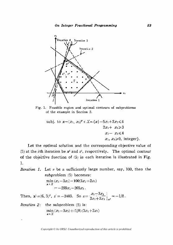
Fig. 1. Feasible region and optimal contours of sub problems of the example in Section 2.
subj. to X=(Xl, X2)T E X={xl-5xl+2x2~4
2Xl+ x2~3
Xl- x2~4
Xl, X2~0, integer}.
53
Let the optimal solution and the corresponding objective value of
(5) at the ith iteration be Xi and Zi, respectively. The optimal contour
of the objective function of (5) in each iteration is illustrated in Fig.
1.
Iteration 1. Let 7r be a sufficiently large number, say, 100, then the
subproblem (5) becomes:
min (xl-3x2)-100(3xl +2X2) XEX
= -299xl-203x2.
Then, xl=(6, 3)T, zl=-2403. So n==: xl-3x2 I =-1/8. 3Xl+2x2 x'
Iteration 2: the subproblem (5) is:
min (XI-3X2)+(1/8) (3Xl +2X2) XEX
Copyright © by ORSJ. Unauthorized reproduction of this article is prohibited.
54 Yuichiro Anzai
= (11/8)Xl-(11/4)X2 .
Then, x2=(2, 6Y, z2=-55/4, and 1r
Iteration 3. the subproblem (5) is:
min (xl-3x2)+(8/9) (3Xl +2X2) XEX
= (11/3)Xl-(11/9)X2 .
Then, x 3=(1, 4Y, z3=-11/9, and 7r=-1.
Iteration 4: the subproblem (5) is:
min (xl-3x2)+(3xl +2X2) xEX
=4Xl-X2.
Then, x4=(1, 4Y, Z4=0. Since the optimal objective value of (5) is
nonnegative, an optimal solution is obtained, which is xl=l, x2=4,
and the optimal objective value is -l.
Extension to multisector problems. Consider the following large-scale
nonlinear integer programming problem, in which p subsystems are
coupled in the fractional objeGtive function:
(6 ) . p[x1+··· +pJxP mln T T
Xl.···.Xp q1 X 1+···+qp x p
subj. to Xi E Xi={XiIAiXi~bi, Xi ";3; 0, integer vector},
i=l,···,p.
We assume that Xi is nonvoid and bounded for all i=l, ... , p, and p
:2jq[Xi>O for Xi E Xi, i=l, ... , p. i=l
Applying the above algorithm to the problem (6), subproblems
(5) become: p p
min :2]p[x;-7r:2]q[x; Xl. ''', xpi=l i=l
subj. to Xi E Xi, i=l, ... , p,
or
(7 ) • T T mlnpi Xi-7rq; Xi X; i=l, .'., p.
subj. to Xi E Xi
Copyright © by ORSJ. Unauthorized reproduction of this article is prohibited.
On Integer Fractional Programming 55
Though (6) is the nonlinearly coupled system, its optimal solution can
be obtained by the iterative solution of p independent linear sub·
problems (7). Sinc.e the efficiency of integer programming algorithms
generally decreases nonlinearly with the increase of the number of
variables, the above machinary may improve the computational effi·
ciency. Actually, the problem (3) is the special case of (6) for p=1.
Rlustrative Example
. -xl-3xi-X3+X4--XS mm --2XI +x2+3x3+5xd-xs
subj. to XI=(XI, X2)T E XI={xl-XI+2x2~9,
4xI+x2~21, ;rl-3x2~0, 4XI+5X2;;;.12,
Xl, X2;;;'0, integer}
X2=(Xa, Xl, x!)T E X2={xl-2x8+6X4~21,
7X3+4x4~39, xs=l, Xs, X4, xs;;;'O, integer}.
Iteration 1: let 'Jr= 100, then the two subproblems (7) become:
subproblem 1: min (-1, -3)xl-1OO(2, l)xl XIEXl
= - 201xI --103x2 .
subproblem 2: min (-1,1, -l)x2-100(3, 5, 1)x2 X2 EX2
= -301xs--499x4-101xs.
Optimal solutions are xl=(4, 5Y, x~=(3, 4, l)T. The sum of the optimal
objective values is z'=zl+zl= -4319.. Then,
(-1, -3)xl+(-1, 1, -l)xl 'Jr=
(2, 1)xl+(3, 5, l)xl -19/43.
Iteration 2: the subproblems (7) are:
subproblem 1: min (-1, -3)Xl +(19/43) (2, l)xl XI E Xl
= -(5/43):cl-(1l0/43)x2 ,
subproblem 2: min (-1,1, -1)x2+(19/43)(3, 5, 1)x2 X2 E X2
= (14/43)xs + (138/43)x4 - (24/43)xs .
Then, xi=(3, 6)T, xl=(O, 0, l)T, and .;::'=zi+zl= -675/43-24/43= -699/43.
And substituting xi and xi into the objective function, we obtain
Copyright © by ORSJ. Unauthorized reproduction of this article is prohibited.
56 Yuichiro Anzai
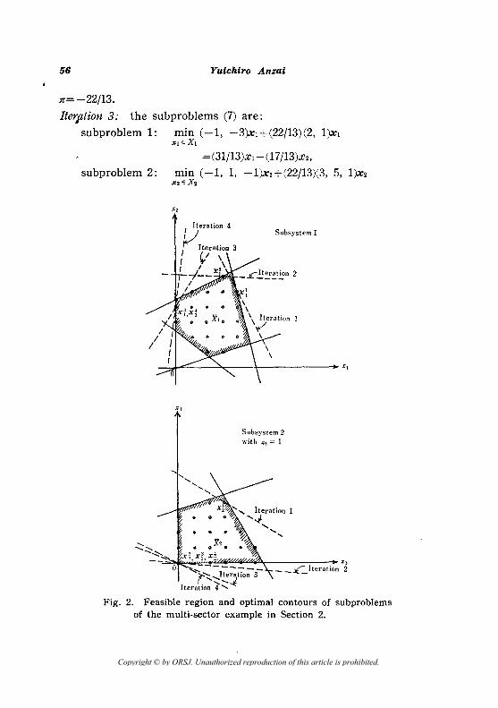
n=-22j13.
Jterption 3: the subproblems (7) are:
subproblem 1: min (-1, -3)Xl +(22/13) (2, l)Xl X,EX,
= (31j13)xl - (17 j13)x2,
subproblem 2: min (-1, 1, -1)x2+(22j13)(3, 5, 1)x2 X2 E X2
Subsystem 1
__ ~~ ____ ~~ ____ .~ ____________ .x,
Subsystem 2 with X5 = 1
.::::, ~~~-~~~~~~~~~~----__ ~--~X3 __ L Iteration 2
Fig. 2. Feasible region and optimal contours of subproblems of the multi-sector example in Section 2.
Copyright © by ORSJ. Unauthorized reproduction of this article is prohibited.
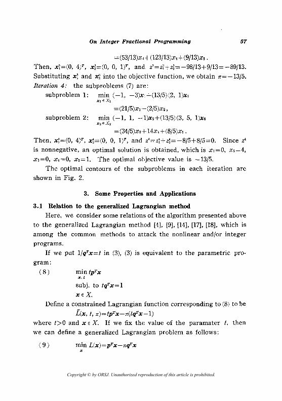
On Integer Fractional Programming 57
= (53/13)x3 + (123/13)x! + (9/13)x5 .
Then, x;=(O, 4)T, x;=(O, 0, I)T, and Z3=Z;+Z;= -98/13+9/13= -89/13.
Substituting x; and r, into the objective function, we obtain rc= -13/5.
Iteration 4: the subproblems (7) are:
subproblem 1: min (-1, -3)xl+(13/5) (2, l)Xl XIEXI
= (21/5)xl --- (2/5)X2 ,
subproblem 2: min (-1,1, -1)x2+(13/5) (3, 5, l)x2 X2 E X2
= (34/5)xa + 14x, + (8/5)xs .
Then, x:=(O, 4Y, x:=(O, 0, l)T, and z'=z:+z;= -8/5+8/5=0. Since z!
is nonnegative, an optimal solution is obtained, which is Xl=O, x2=4,
X3=0, x,=O, xs=l. The optimal objective value is -13/5.
The optimal contours of the subproblems in each iteration are
shown in Fig. 2.
3. Some Properties and Applications
3.1 Relation to the generalized Lagrangian method
Here, we consider some relations of the algorithm presented above
to the generalized Lagrangian method [4], [9], [14], [17], [18], which is
among the common methods to attack the nonlinear and/or integer
programs.
If we put l/qTx=t in (3), (3) is equivalent to the parametric pro
gram:
(8) min tpTx x, t
subj. to tqTx= 1
XEX.
Define a constrained Lagrangian function corresponding to (8) to be
i(x, t, rc)=tpTx-rc(tqTx-1)
where t>O and x E X. If we fix the value of the paramater t, then
we can define a generalized Lagrangian problem as follows:
(9) min L(x)=pTx-rcqTx x
Copyright © by ORSJ. Unauthorized reproduction of this article is prohibited.
58 Yuichiro Anzai
subj. to X E X.
Since X is a nonvoid, finite set, a finite optimal solution of (9) exists
for any n.
In general, the procedures to change the values of multipliers in
generalized Lagrangian methods are essentially trial and error, and
solving Lagrangian problems may not provide the solution of the
original problem whatever the values of multipliers are changed.
However, note that (9) is just the sub problem (5) solved in our
algorithm. Furthermore, it can be easily verified that an optimal
solution of (9), x(n), is an optimal solution of (8) where the parameter
t is fixed to be l/qTx(n). Thus, the algorithm presented in Section 2
may be considered as the finite procedure to solve the Lagrangian
problem (9) by suitably changing the value of n. In other words,
our algorithm can also be classified as the generalized Lagrangian
method with the finite convergence.
3.2 Relation to the continuous fractional programming algorithms
The proposed algorithm can be modified to solve the continuous
linear fractional programs (1) if X is bounded as will be shown below.
We assume that r=s=O in (1) without loss of generality and X is
bounded in this section.
It is well known that the optimum of (1) occurs at an extreme
point of X [19]. Thus, defining X={xlx E X, x is a basic feasible
solution}={xl, ... , X S}, an optimal solution of (4) provides an optimal
solution of (1). The column to enter the basis in each simplex itera
tion of the solution of (4) is determined by min pTxk-nqTx'<, however, k
it can be found by solving the linear subproblem:
(10) minpTx-nqTx .le
subj. to x EX,
since Xk is an extreme point of X. Hence, the global optimum of (1)
can be obtained directly by the proposed algorithm.
Copyright © by ORSJ. Unauthorized reproduction of this article is prohibited.
On Integer Fractional Programming 59
Since the optimum can be obtained at an extreme point of the
feasible region in continuous fractional programs, some pivoting
algorithms to search neighboring extreme points have been proposed
in [12], [19]. Let us compare those with our method.
Adding to constraints the equations related to the denominator and the numerator:
2:: qjXj-ZI=O j
2:: PjXj-Z2=0 j
and describing them in the canonical form related to some feasible basis, the equations can be written as follows:
+ + +
x'" +am, m+IX",+I + ... + a",,,x,, = b", -Zl +qm+I;Cm+I +···+q"x" =-Zl
-Z2 +pm+l.rm+l +···+p"x" =-Z2. Pivoting at ars, new values of Zl, ZI: are
-ZI=-ZI-8qs -Z2= -z2-8ps
where 8=br/ars>0. Then the value of the fractional objective becomes
z2+8ps zl+8q~ .
The objective value is improved when Z<Z2/ZI, i.e.,
z2+8ps Zl +8ijs
or, since Zl +8q.>0, 8>0,
(11) c.=P.-(Z2/ZI)q.<0.
The column to enter the basis is determined by min Cj. If Cj;;;;'O for J
Copyright © by ORSJ. Unauthorized reproduction of this article is prohibited.
60 Yuichiro Anzai
all j, then the optimal solution with ZI, Z2 provides the optimum of (1).
Note that Cj is just the cost coefficient of Xj in our subproblem
(10). So the above procedure searches locally a good extreme point
of X, but our method searches globally by resolving the linear pro·
gram (10), both using the relative cost factor (11).
The relative cost factor (11) is slightly different from ones in
Gilmore and Gomory [12] or Swarup [19]. Since O/(ZI +01js) is eliminated
in (11), min Cj need not provide the best neighboring extreme point. j
This situation occurs in the same way as in [19], but, in [12], the best
direction is searched by using directional derivatives.
By the above reason, comparing to the other methods, ours is not
the locally steepest descent method. Furthermore, different from [12]
or [19], several linear programs should be solved in our method, though
the primal simplex method can be effectively used by considering re
as the cost parameter.
3.3 Relation to the vector optimum problems
As fractional programming is a relative optimization problem, it
is naturally related to the optimization problems with multiple objec
tives as follows [11]:
(12) max (f1(X), "', j m,(X» JC
subj. to x E Xt;;E'" where ji(X) is an arbitrary function of x.
A common concept of optimality for such a problem is Pareto
optimality.
Definition. x E X is said to be a Pareto optimal solution of (12) if there
exists no XEX such that ji(X);:.ji(X) for all i=l, "', m and j,,(x»
j,,(x) for some h such that l~h~m.
The relation between our problem (3) and the problems of the
type (12) is specified as follows.
Theorem 2. Consider the vector optimum problem:
Copyright © by ORSJ. Unauthorized reproduction of this article is prohibited.
On Integer Fractional Programming 61
(13) max (jl(X) = _pTX, j2(X)=qTX)
'" subj. to xEX={x!Ax",;b, x~o, integer vector}
where jl(X)~O, j2(X»O for all x EX.
Then an optimal solution of (3), x*, is a Pareto optimal solution of
(13).
Proof. Suppose that x* is not a Pan~to optimal solution of (13). Then
there exists x E X such that jl(X) > fl(X*) and j2(X)~ j2(X*), or jl(X)~
jl(X*) and j2(X) > j2(X*). For both cases,
That is,
_jl(X*»_jl~) f * - X or x ,XE . j2(X*) j2(X)
It contradicts the assumption that .x* is an optimal solution of (3).
Note that the above result holds also if the feasible region is g, for the definition of Pareto optimality does not depend on topological
properties of X or jt(x).
3.4 Application to goal programming Fractional programming is essentially a relative optimization of
the numerator and denominator function. Hence, as an important
field to which it is applicable is the optimization of efficiency. For
example, a multi-item production scheduling to maximize the rate of
return under the resource and demand constraints. Another example
is referred to by Gilmore and Gomory in cutting stock problems in
the paper industries [12]. However, in fact, the maximization or mini
mization of "efficiency" is sometimes meaningless. On the contrary,
the goal attainment of efficiency is not only meaningful, but it is
sometimes the more practical objective in actual social systems than
ones such as the maximization of total profits or the minimization of
total costs.
Here, a goal attainment problem of the total rate of return in a
Copyright © by ORSJ. Unauthorized reproduction of this article is prohibited.
62 Yuichiro Anzai
capital budgeting problem for the project selection is formulated as
the 0-1 integer linear fractional program, and solved by the proposed
algorithm.
The goal programming problem to select projects from n condidate
projects such that expected profit/total capital investment is closest
to the given goal value of the rate of return under the constraints of
upper and lower bounds of the total capital investment and the variance
of profit can be formulated as follows:
n
. 2: p,X, (14) min I ':' A
Xl' •••• xn'L,CiXi i=l
n subj. to CL~ 2: c,x,~Cu
i=l n
:ZWiXi~V i=l
x,=O or 1, i=l, ... , n, n
where w,=v,c,/ 2: C,Xi, pi=r,C" i=l
and e,: capital investment for the ith project
r,: expected rate of return of the i th project
v,: variance of rate of return of the ith project
Cu: upper bound of the available total capital
CL: lower bound of the available total capital
V: upper bound of the sum of weighted variance
of profit
A: goal value of rate of return.
Note that xi=1 if the ith project is selected and x,=O if not.
An optimal solution of (14) can be obtained by solving the follow
ing two 0-1 fractional programs:
n
±{:z (r,-Aci)x,} (15) min
i=l
n :Zc,x, i=l
Copyright © by ORSJ. Unauthorized reproduction of this article is prohibited.
On Integer Fractional Programming 63
n
subj. to GL~ .2: CiXi~GU i=l
n .2: (Vi- V)CiXi:;;;;O i=l
n ± { .2: (ri-ACi)Xi}>O
i=l
Xi=O or 1, i=l, "', n.
The above problems can be solved by the proposed algorithm,
where the subproblems (5) become 0-1 linear programs.
The computational result of an example problem with 12 projects
Table 1. Data for the project selection problem.
Project No. Capital Expected Variance of investment rate of return rate of return
1 47.0 0.17 0.0060 2 55.0 0.25 0.0045 3 86.0 0.20 0.0058 4 23.0 0.41 0.0033 5 98.0 0.59 0.0125 6 25.0 0.33 0.0050 7 74.0 0.48 0.0100 8 74.0 0.35 0.0088 9 70.0 0.08 0.0015
10 45.0 0.27 0.0045 11 93.0 0.15 0.0075 12 55.0 0.56 0.0090
Parameters: G=200.0, G=125.0, V=O.007.
Table 2. Computational results for the project selection problem.
Goal value Projects Total Expected Expected of rate of capital rate of I(A)-(B)I return (A) selected investment profit return (B)
0.1 9, 11 163.0 19.6 0.120 0.020 0.2 4, 9, 10 138.0 27.2 0.197 0.003 0.3 4, 9, 10, 12 193.0 58.0 0.300 0.000 0.4 2, 4, 12 133.0 54.0 0.406 0.006 0.5 4, 6, 10, 12 148.0 60.6 0.410 0.090 0.6 4, 6, 10, 12 148.0 60.6 0.410 0.190
Copyright © by ORSJ. Unauthorized reproduction of this article is prohibited.
64 Yuichiro Anzai
is tabulated in Tables 1 and 2. Subproblems are solved by Balas'
additive algorithm [1] and the average execution time for one case is
about 30-40 secs (IBM 7040, FORTRAN IV).
Note that (14) is essentially different from the problem with the
objective function, minimize \ ~;PiXi-A~CiXi \. They have been
sometimes confounded with in practical systems. 0-1 fractional pro·
gramming algorithms were treated with by Ivanescu and Rudeaunu
[13], but they considered basically the problems such that every term
in the denominator has the plus sign and there are no constraints
except 0-1 conditions.
Comments
1. As in nonlinear programming, it would be more popular to
solve integer nonlinear programs by the iterative solution of integer
linear subproblems (Benders' partitioning method [3] is a typical ex
ample). Thus, the presented algorithm, which provides the solution
of integer nonlinear programs, also suggests one of the main direc
tions to attack formidable integer nonlinear programming, though it
does not conquer the difficulties of handling with linear integer pro
grams.
2. Note that only the finiteness property of X is used in the
construction of subproblems (5). This implies that, even if X in (3)
is characterized as a finite set of another type, it is sufficient that
practically solvable sub problems are constructed. It makes very wide
the applicability of the algorithm.
Acknowledgement
The author thanks Associate Professors K. Shimizu and H. Yanai
of Keio University for their helpful suggestions.
References
[1] Balas, E., "An Additive Algorithm for Solving Linear Programs with Zero-
Copyright © by ORSJ. Unauthorized reproduction of this article is prohibited.
On In teger Fractional Programming 65
one Variables," Opns. Res., 13 (1965), 517-544. [2] Bector, C.R., "Programming Problems with Convex Fractional Functions,"
Opns. Res., 16 (1968), 383-391. [3] Benders, J.F., "Partitioning Procedures for Solving Mixed-Variables Pro
gramming Problems," Numerische Mathematik, 4 (1962), 238-252. [ 4] Brooks, R. and A. Geoffrion, "Finding Everett's Lagrange Multipliers by
Linear Programming," OPns. Res., H (1966), 1149-1153. [5] Charnes, A. and W.W. Cooper, "Programming with Linear Fractional
Functionals," Naval Res. Log. Quart., 9 (1962), 181-186. [6] Charnes, A. and W.W. Cooper, "Programming with Linear Fractional
Functionals, A Communication," Nal'al Res. Log. Quart., 10 (1963), 273-274. [7] Cord, J., "A Method for Allocating Funds to Investment Projects when
Returns are subject to Uncertainty," Management Sci., 10 (1964) 335-341. {8] Dantzig, G.B., Linear Programming and Extensions, Prinston Univ. Press,
N.J., 1963. [9] Everett HI, H., "Generalized Lagrange Multiplier Method," Opns. Res., 11
(1963), 399-417. [10] Fogler, H.R., "Ranking Techniques and Capital Budgeting," The Accounting
Review, XLVII (1972), 134-143. [11] Geoffrion, A., "Solving Bicriterion Mathematical Programs," Opns. Res., 15
(1967), 39-54. [12] Gilmore, P.C. and R.E. Gomory, "A Linear Programming Approach to the
Cutting Stock Problem-Part H," OPns. Res., 11 (1963), 863-888. [13] Ivanescu, P.L. and S. Rudeaunu, "Pseudo-Boolean Methods for Bivalent
Programming," Lecture Notes in l'vtathematics, Vo!. 23, Springer-Verlag. Berlin-Heidelberg-New York, 1966.
[14] Jagannathan, R., "On Some Properties of Programming Problems in Parametric Form Pertaining to Fractional Programming," Management Sci., 12 (1966), 609-615.
[15] Joksch, H., "Programming with Fractional Linear Objective Functions," Naval Res. Log. Quart., 11 (1964), 19?-204.
[16] Martos, S., "Hyperbolic Programming," Naval Res. Log. Quart., 11 (1964). 135-155.
[17] Nemhauser, G. and Z. Ullman, "A Note on the Generalized Lagrange Multiplier Solution to an Integer Programming Problem," OPns. Res., 16 (1968), 450-452.
[18] Shapiro, J.F., "Generalized Lagrange Multipliers in Integer Programming," OPns. Res., 19 (1971), 68-76.
[19] Swarup, K., "Linear Fractional Functionals Programming," Opns. Res., 13 (1965), 1029-1036.
[20] Swarup, K., "Fractional Programming with Non-linear Constraints," Z.A.M.M., 46 (1966), 468-469. As for nonlinear fractional programming,
Copyright © by ORSJ. Unauthorized reproduction of this article is prohibited.
66 Yuichiro Anzai
see also Gupta, R.K. and K. Swarup, Z.A.M.M., 49 (1969), 753-756, and Anand, P. and K. Swarup, Z.A.M.M., 50 (1970), 320-321.
[21] Swarup, K., "Some Aspects of Duality for Linear Fractional Functionals Programming," Z.A.M.M., 47 (1967), 204-205.
[22] Weingartner, H.M., "Capital Budgeting of Interrelated Projects: Survey and Synthesis," Management Sei., 12 (1966), 485-516.
Copyright © by ORSJ. Unauthorized reproduction of this article is prohibited.