on modular and cusp forms with respect to the congruence ... · the congruence subgroup, over which...
TRANSCRIPT

On modular and cusp forms with respect tothe congruence subgroup, over which themap given by the gradients of odd Thetafunctions in genus 2 factors, and related
topics
Alessio Fiorentino
Thesis Advisor
Prof. R. Salvati Manni

2
Contents
1 The Siegel Upper Half-plane and the Simplectic Group 111.1 The Symplectic Group . . . . . . . . . . . . . . . . . . . . . . . . 111.2 Congruence subgroups of the Siegel modular group . . . . . . . 131.3 Action of the Symplectic Group on the Siegel Upper Half-Plane 17
2 Siegel Modular Forms 232.1 Definition and Examples . . . . . . . . . . . . . . . . . . . . . . . 232.2 Fourier series of a modular form . . . . . . . . . . . . . . . . . . 262.3 Cusp forms . . . . . . . . . . . . . . . . . . . . . . . . . . . . . . . 31
3 Theta constants 353.1 Characteristics . . . . . . . . . . . . . . . . . . . . . . . . . . . . . 353.2 k-plets of even 2-characteristics . . . . . . . . . . . . . . . . . . . 383.3 Theta constants . . . . . . . . . . . . . . . . . . . . . . . . . . . . 433.4 Jacobian determinants . . . . . . . . . . . . . . . . . . . . . . . . 553.5 Classical structure theorems . . . . . . . . . . . . . . . . . . . . . 573.6 A new result: another description for χ30 . . . . . . . . . . . . . 593.7 Rings of modular forms with levels . . . . . . . . . . . . . . . . . 63
4 The group Γ and the structure of A(Γ) and S(Γ) 674.1 The Theta Gradients Map . . . . . . . . . . . . . . . . . . . . . . 674.2 The congruence subgroup Γ . . . . . . . . . . . . . . . . . . . . . 684.3 Structure of A(Γ): generators . . . . . . . . . . . . . . . . . . . . . 724.4 Structure of A(Γ): relations . . . . . . . . . . . . . . . . . . . . . . 74
4.4.1 Relations among θ2mθ
2n . . . . . . . . . . . . . . . . . . . . 74
4.4.2 Relations among D(N) . . . . . . . . . . . . . . . . . . . . 754.4.3 Relations among D(N) and θ2
mθ2n . . . . . . . . . . . . . . 79
4.5 The Ideal S(Γ)e . . . . . . . . . . . . . . . . . . . . . . . . . . . . . 86
A Elementary results of matrix calculus 87
B Satake’s compactification 91B.1 Realization of Sg as a bounded domain . . . . . . . . . . . . . . 91B.2 Boundary Components . . . . . . . . . . . . . . . . . . . . . . . . 93B.3 The cylindrical topology on Drc
g . . . . . . . . . . . . . . . . . . . 96
Bibliografia 98
3

4 CONTENTS

Introduction
The theory of automorphic functions rose around the second half of the nine-teenth century as the study of functions on a space, which are invariant underthe action of a group and consequently well defined on the quotient space.
The so-called elliptic functions, for which the first systematical expositionwas given by Karl Weierstrass, are one of the simplest examples of automorphicfunctions. These are meromorphic functions of one variable with two indepen-dent periods and can be regarded, therefore, as functions on the complex torusC/L, where L is the lattice generated by the two periods 1.
A first classical generalization of this notion is suggested by working withfunctions defined on isomorphism classes of complex tori. Since there existsa bijection between the isomorphic classes of complex tori and the points ofthe quotient space H/SL(2,Z) 2, where H is the complex upper half-plane, aremarkable example pertaining to the theory of automorphic functions is pro-vided by holomorphic functions on H, which are invariant under the action ofSL(2,Z); this is what is meant by a modular function 3.
More in general, the classical theory of the so-called elliptic modular formspertained to the study of holomorphic functions onH, which transform underthe action of a discrete subgroup of SL(2,R) as a multiplication by a factorsatisfying the 1-cocycle condition. In the first half of the twentieth centuryCarl Ludwig Siegel was the first to generalize the elliptic modular theory tothe case of more variable, by discovering some prominent examples of au-tomorphic functions in several complex variables; these are named after himSiegel modular forms. In this theory ([F], [Kl], [VdG]), H is generalized by theupper half-plane Sg B
{τ ∈ Sym(g,C) | Imτ > 0
}and a transitive action of the
symplectic group Sp(2g,R) is defined on Sg, thus generalizing the action ofSL(2,R) onH:
1A classical result completely describes these functions by means of the Weierstrass ℘-functionand its derivative; the elementary theory is detailed, for instance, in [FB]
2See, for instance, [FB].3Thanks to a classical result, the field of modular functions is known to be generated by the
so-called absolute modular invariant, discovered by Felix Klein in 1879 (see Chapter 2, Example2.3)
5

6 CONTENTS
Sp(2g,R) ×Sg −→ Sg( (A BC D
), τ
)→ (Aτ + B) · (Cτ + D)−1
The arithmetic subgroup Γg B Sp(2g,Z) plays, in particular, a meaningful roleaccording to this action from a geometrical point of view, since the points of thequotient space Ag B Sg/Γg describe the isomorphism classes of the principallypolarized abelian varieties 4.
Modular forms can be used as coordinates in order to construct suitableprojective immersions of level quotient spaces with respect to the action ofremarkable subgroups of the group Γg. Riemann Theta functions with charac-teristics:
θm(τ, z) B∑n∈Zg
eπi[
t(n+ m′2 )τ(n+ m′
2 )+2t(n+ m′2 )(z+ m′′
2 )]
are, in particular, are a good instrument at disposal of the theory, in order toconstruct suitable modular forms, because the so-called Theta constants:
θm(τ) B θm(τ, 0)
and the Jacobian determinants:
D(n1, . . . ,ng)(τ) B
∣∣∣∣∣∣∣∣∣∣∂∂z1θn1 | z=0 (τ) . . . ∂
∂zgθn1 | z=0 (τ)
......
∂∂z1θng | z=0 (τ) . . . ∂
∂zgθng | z=0 (τ)
∣∣∣∣∣∣∣∣∣∣turn out to be modular forms with respect to a technical level subgroupΓg(4, 8) ⊂ Γg. A remarkable map can be defined in particular on the levelmoduli space A4,8
g B Sg/Γg(4, 8), whose image lies in the Grassmannian of g-dimensional complex subspaces inC2g−1(2g
−1)and whose Plucker coordinates arethe Jacobian determinants:
PgrTh : A4,8g −→ GrC(g, 2g−1(2g
− 1))
In their paper [GSM] Samuel Grushevski and Riccardo Salvati Manni provedthat the map PgrTh is generically injective whenever g ≥ 3 and injective ontangent spaces when g ≥ 2.The map is conjectured to be injective whenever g ≥ 3, albeit it has not beenproved yet. On the other hand, when g = 2, the map:
4See, for instance, [GH], [De] or [SU]
CONTENTS 7
PgrTh : A4,8−→ P14
is known not to be injective.
In this thesis, a description is provided for the congruence subgroup Γ suchthat the the map PgrTh in genus 2 is still well defined on the correspondentlevel moduli space AΓ B Sg/Γ and also injective. It is also proved that Γ isa normal subgroup of Γ2 with no fixed points; hence, the correspondent levelmoduli space AΓ turns out to be smooth.A structure theorem is also proved for the even part of the rings of the gradedrings of modular forms A(Γ) and for the even part of the ideal of cusp formsS(Γ) (namely the modular forms which vanish on the boundary of Satake’scompactification) with respect to Γ. These are, indeed, the only parts whichcounts in studying the geometry of the desingularization of the map on theboundary of Satake’s compactification. Alas, a geometrical description stillmisses, due to the the not simple structure of A(Γ) and S(Γ).
Chapters 1 and 2 are designed to provide an outline of the basic theory; thereader is obviously referred to the bibliography for a deeper knowledge of thetopics.
Chapter 3 is mainly focused on Theta constants and related topics. Section3.6 is, in particular, devoted to a new description found for a known modularform of weight 30 in genus 2, which is characterized by transforming with anon-trivial character under the action of Γ2.
Chapter 4 is, finally, centered around the above mentioned results concern-ing the group Γ.
The author wishes to thank Professor Salvati Manni for his help. He alsoseizes the opportunity to thank Professor Freitag for having performed somenecessary computations by means of a computer program written by him.

8 CONTENTS

Notation
For each set A the symbol |A| will stand for its cardinality. The symbol A ⊂ Bwill mean that A is a subset of B, which is not necessarily proper. To state thatthe set A is a proper subset of B, the symbol A ( B will be used.For an associative ring with unity R, the symbol M(g,R) will denote the g × gmatrices, whose entries are elements of R, while the symbol Symg(R) will standfor the symmetric g × g matrices.For a field F, GL(g,F) and SL(g,F) will stand respectively for the general lineargroup of degree n and for the special linear group of degree n.The symbol Sn will stand for the symmetric group of order n!.The exponential function eπiz will be denoted by the symbol exp(z).
9

10 CONTENTS

Chapter 1
The Siegel Upper Half-planeand the Simplectic Group
A more exhaustive discussion concerning these topics can be found in Siegel’sclassical work [Si], as well as in Freitag’s book [F] and Klingen’s book [Kl],where a focus on Minkowski’s reduction theory is also available. Most of thetopics are also outlined in Namikawa’s Lecture notes [Na], where Satake’s andMumford’s compactifications of the quotient space are discussed.
1.1 The Symplectic Group
Definition 1.1. The symplectic group of degree g is the following subgroup ofGL(2g,R):
Sp(g,R) B={γ ∈M(2g,R) | tγ · Jg · γ = Jg
}where:
Jg =
(0 1g−1g 0
)is the so called symplectic standard form of degree g.
The symplectic group naturally arises as the group of the automorphisms ofthe lattice Z2g, provided with the form Jg
1; as it clearly turns out from thedefinition, it is an algebraic group.A generic element of the symplectic group can be depicted in a standard blocknotation as:
γ =
(aγ bγcγ dγ
)aγ, bγ, cγ, dγ ∈M(g,R)
1More in general, a symplectic group Sp(g,Λ) can be defined, whose elements are the lineartransformations preserving a given non-degenerate skew-symmetric bilinear form Λ of degree 2;such transformations are in fact named symplectic transformations.
11

12CHAPTER 1. THE SIEGEL UPPER HALF-PLANE AND THE SIMPLECTIC GROUP
By expliciting the conditions describing the elements of the group, one has:
Sp(g,R) =
{γ ∈ GL(2g,R |
taγcγ = tcγaγtbγdγ = tdγbγ
; taγdγ − tcγbγ = 1g
}=
=
{γ ∈ Gl(2g,R) | γ−1 = J−1
gtγJg =
(tdγ −
tbγ−
tcγ taγ
)} (1.1)
As it immediately turns out, the symplectic group is stable under the transpo-sition γ → tγ; thus, an equivalent characterization follows, by expliciting theconditions for the transposed element:
Sp(g,R) =
{γ ∈ GL(2g,R |
aγtbγ = bγtaγcγtdγ = dγtcγ
; aγtdγ − bγtcγ = 1g
}(1.2)
The following definition introduces a remarkable subgroup of Sp(g,R), onwhich the theory focuses:
Definition 1.2. The subgroup:
Γg B Sp(g,Z) ={γ ∈ Sp(g,R) | aγ, bγ, cγ, dγ ∈M(g,Z)
}= Sp(g,R)∩M(2g,Z)
is called the Siegel modular group of degree g 2. When g = 1, the group Γ1 =SL(2,Z) is called the elliptic modular group 3
Proposition 1.1. The set:
S B{
Jg ,
{(1g S0 1g
)}S∈Symg(Z)
}is a set of generators for the modular group Γg.
Proof. For each η ∈ Γ1 and h = 1, . . . g, let A(g)η,h be the 2g × 2g matrix, whose
entries are:
(A(g)η,h)i j =
aη − 1 if i = j = h;bη if i = h, j = h + g;cη if i = h + g, j = h;dη − 1 if i = j = h + g;0 otherwise
Then:
γ(g)η,h B 12g + A(g)
η,h ∈ Γg ∀η ∈ Γ1, ∀h = 1, . . . g
2One can observe that Γg is an example of arithmetic subgroup of Sp(g,R)3A classical result states that Γ1/{±1} is the group of the biholomorphic automorphisms of the
Riemann sphere C.

1.2. CONGRUENCE SUBGROUPS OF THE SIEGEL MODULAR GROUP 13
By multiplying γ ∈ Γg by suitable elements of the kind γ(g)η,h from the left, it can
be checked that the matrix:
Nγ =
(u 00 tu−1
)∏η,h
γ(g)η,h γ
with a suitable u ∈ GLg(Z), has the unit vector eg+1 as (g + 1)-th column. Sinceγ ∈ Γg, the first row of Nγ have to be e1. Then, by induction, one concludes thatthe group Γg is generated by:
{{γ(g)η,h}η,h ,
{(u 00 tu−1
)}u∈GLg(Z)
,
{(1g S0 1g
)}S∈Symg(Z)
}However, it is easily checked that the elements γ(g)
η,h are generated by the otherelements and Jg. Therefore, the modular group turns out to be generated bythe set:
{Jg ,
{(u 00 tu−1
)}u∈GLg(Z)
,
{(1g S0 1g
)}S∈Symg(Z)
}Moreover, for each u ∈ GLg(R) one has:
(u 00 tu−1
)=
(1g u0 1g
) (0 1g−1g 0
) (1 u−1
0 1
) (0 1g−1g 0
) (1g u0 1g
) (0 1g−1g 0
)and, therefore, the thesis follows. �
Corollary 1.1. The modular group Γg is also generated by matrices of the form:
γ =
(aγ bγ0 dγ
), tγ−1 =
(dγ 0−bγ aγ
)tbγdγ = tdγbγ ; taγdγ = 1g
Proof. Thanks to Proposition 1.1, one has only to check that the set S is generatedby such matrices. However, since:
Jg =
(1g 0−1g 1g
) (1g 1g0 1g
) (1g 0−1g 1g
)the thesis easily follows.
�
1.2 Congruence subgroups of the Siegel modulargroup
The aim of this section is to introduce some remarkable subgroups of the Siegelmodular group Γg, which reveal themselves to be a natural tool to generalizethe notion of modular functions.

14CHAPTER 1. THE SIEGEL UPPER HALF-PLANE AND THE SIMPLECTIC GROUP
Definition 1.3. For each n ∈ N let Γg(n) be the kernel of the natural homomorphismΓg → Sp(g,Z/nZ), induced by the canonical projection. Γg(n) is known as theprincipal congruence subgroup of level n.
As a kernel of a group homomorphism, Γg(n) is a normal subgroup of Γg.Moreover, since:
Γg(n) = {γ ∈ Γg | γ ≡ 12g modn}
an immediate characterization can be derived:
Γg(n) ={γ ∈M(2g,Z) | γ ≡ 12g + nMγ
}
with Mγ =
(aM bMcM dM
)s.t.
tbM = bM + n(tdMbM −
tbMdM)
tcM = cM + n(taMcM −tcMaM)
dM + taM + n(taMdM −tcMbM) = 0
(1.3)
It is a remarkable property of such subgroups that they are of finite index inthe Siegel modular group; in particular, the following Lemma holds:
Lemma 1.1. For each n ∈ N:
[Γg : Γg(n)] = ng(2g+1)∏p|n
∏1≤k≤g
(1 −
1p2k
)Proof. A proof can be found in [Ko]. �
Pertaining principal congruence subgroup with even level, some elementarylemmas can be stated:
Lemma 1.2. If γ ∈ Γg(2n), γ2∈ Γg(4n).
Proof. Let γ1 = 12g + 2nM1, γ2 = 12g + 2nM2 ∈ Γg(2n) with reference to thenotation introduced in (1.3). Then, one has:
γ1γ2 = 12g + 2n(M1 + M2 + 2nM1M2) (1.4)
hence, the thesis follows. �
Lemma 1.3. For each γ ∈ Γg(2n):
diag(taγcγ) ≡ diag(cγ) mod4n diag(tbγdγ) ≡ diag(bγ) mod4n
Proof. Using again the notation introduced in (1.3), one has the following simplechain of congruences:
diag(taγcγ) = diag[t(1g + 2naM) · 2ncM] = diag[2ncM + 4n2(taMcM)] =
= 2n diag(cM) + 4n2diag(taMcM) ≡ 2n diag(cM) mod4n
which proves the first relation, since cγ = 2ncM. Likewise, the second relationis proved. �

1.2. CONGRUENCE SUBGROUPS OF THE SIEGEL MODULAR GROUP 15
Definition 1.4. A subgroup Γ of Γg, such that Γg(n) ⊂ Γ for some n ∈ N is called acongruence subgroup of level n.
Remarkable examples of proper congruence subgroups (namely congruencesubgroups which are not principal) of level n are clearly given by the followingfamily:
Γg,0(n) B{γ ∈ Γg | cγ ≡ 0 modn
}(1.5)
A notable family of congruence subgroups, on which this work mainlyfocuses, is the following one:
Γg(n, 2n) B{γ ∈ Γg(n) | diag(taγcγ) ≡ diag(tbγdγ) ≡ 0 mod2n
}=
={γ ∈ Γg(n) | diag(aγtbγ) ≡ diag(cγtdγ) ≡ 0 mod2n
}It is immediately seen that Γg(2n) ⊂ Γg(n, 2n); therefore, such subgroups arecongruence subgroups of level 2n. Moreover, Lemma 1.3 implies the character-ization:
Γg(2n, 4n) ={γ ∈ Γg(2n) | diag(bγ) ≡ diag(cγ) ≡ 0 mod4n
}(1.6)
The congruence subgroups of the type (1.6) satisfy some notable properties:
Lemma 1.4. If γ ∈ Γg(2n, 4n), γ2∈ Γg(4n, 8n).
Proof. Let γ = 12g + 2nM be as in (1.3); then, the thesis follows from (1.4), sincefor hypothesis diag(bM) ≡ diag(cM) ≡ 0 mod2. �
Proposition 1.2. The congruence subgroup Γg(2n, 4n) is normal in Γg for each n ∈ N.Moreover, [Γg(2n) : Γg(2n, 4n)] = 22g.
Proof. Let γ = 12g + 2nM be, as in (1.3), the generic element of Γg(2n); then foreach n one can define the map:
Dn : Γg(2n) −→ Zg2 ×Z
g2
γ −→ (diag(bM) mod2, diag(cM) mod2)
Due to (1.4), Dn is a group homomorphism. Moreover the condition Dn(γ) = 0 isequivalent to diag(bγ) ≡ diag(cγ) ≡ 0 mod4n; therefore Γg(2n, 4n) is the kernel ofDn; in particular, Γg(2n, 4n) is normal in Γg(2n). In order to prove that Γg(2n, 4n)is normal in Γg, one has to prove that ηγη−1
∈ KerDn whenever γ ∈ Γg(2n, 4n)and η ∈ Γg. One has:
ηγη−1 =
(aη bηcη dη
) [(1g 00 1g
)+ 2n
(aM bMcM dM
)] (tdη −
tbη−
tcη taη
)= 12g + 2n
(a′ b′
c′ d′
)
16CHAPTER 1. THE SIEGEL UPPER HALF-PLANE AND THE SIMPLECTIC GROUP
where, for instance, b′ = aηbMtaη − bηcM
tbη + t(aηtdMtbη) − (aηaM
tbη); by (1.3)aM + tdm ≡ 0 mod2n, hence:
diag(b′) ≡ aη · diag(bM) + bη · diag(cM) mod2
Since γ ∈ KerDn, it follows that diag(b′) ≡ 0 mod2; likewise one has diag(c′) ≡0 mod2.To prove the second part of the statement, one observes that Dn is also surjective.In fact, for (ε1, ε2) ∈ Zg
2 ×Zg2 , by (1.3) one can choose γ1 ∈ Γg(2n) and γ2 ∈ Γg(2n)
satisfying respectively aM1 = cM1 = dM1 = 0 and diag(bM1 ) ≡ ε1 mod2, and aM2 =bM2 = dM2 = 0 and diag(cM2 ) ≡ ε2 mod2. Then, D(γ1) = (ε1, 0) e D(γ2) = (0, ε2),and the surjectivity of Dn follows, because D(γ1γ2) = (ε1, ε2). Therefore, thefollowing isomorphism is given:
Γg(2n)/Γg(2n, 4n) � (Z2)2g
and consequently [Γg(2n) : Γg(2n, 4n)] = 22g. �
Proposition 1.3. Γg(2n, 4n)/Γg(4n, 8n) is a g(2g + 1)-dimensional vector space onZ2.
Proof. Lemma 1.4 implies that each element in Γg(2n, 4n)/Γg(4n, 8n), whichdiffers from identity, has order 2. Γg(2n, 4n)/Γg(4n, 8n) is, in particular, anabelian group. By Lemma 1.1 and Proposition 1.2, one immediately has[Γg(2n, 4n) : Γg(4n, 8n)] = 2g(2g+1). Then:
Γg(2n, 4n)/Γg(4n, 8n) � Zg(2g+1)2 (1.7)
and the thesis follows. �
Proposition 1.4. For each couple of indices 1 ≤ i, j ≤ g one can denote by Oi j thematrix g × g, whose coordinates are O(hk)
i j = δihδ jk. Then, the following matrices:
Ai j B
(ai j 00 ta−1
i j
)(1 ≤ i, j ≤ g) con ai j B
{1g + 2Oi j se i , j1g − 2Oi j se i = j
Bi j B
(1g bi j0 1g
)(1 ≤ i ≤ j ≤ g) con bi j B
{2Oi j + 2O ji se i , j2Oi j se i = j
Ci j B tBi j (1 ≤ i ≤ j ≤ g)
are a set of generators for Γg(2).
Proof. A proof can be found in [I3]. �
As a consequence of Proposition 1.4 one has the following Corollary:
Corollary 1.2. The g(2g+1) elements Ai j (for i, j , g),Bi j,Ci j (for i < j),B2ii,C
2ii,−12g
are a basis for the Z2 - vector space Γg(2, 4)/Γg(4, 8).
Proof. Thanks to the characterization (1.6), the elements Ai j (i, j , g),Bi j,Ci j (i <j),B2
ii,C2ii are plainly checked to belong to Γg(2, 4). Moreover it can be straightly
verified that such elements belong to distinct independent cosets of Γg(4, 8) inΓg(2, 4). Then, the thesis follows from Proposition 1.3. �

1.3. ACTION OF THE SYMPLECTIC GROUP ON THE SIEGEL UPPER HALF-PLANE17
Another important family of remarkable congruence subgroups this workwill focus on defined by:
Γg(n, 2n, 4n) B{γ ∈ Γg(2n, 4n) | Tr(aγ) ≡ g mod4n
}(1.8)
In the next section the main properties of the action of these subgroups on ameaningful tubular domain of the complex euclidean space will be discussed.
1.3 Action of the Symplectic Group on the SiegelUpper Half-Plane
Definition 1.5. The Siegel Upper Half-Plane of degree g is the following subset:
Sg B{τ ∈ Symg(C) | Imτ > 0
}(1.9)
The Siegel upper half-plane clearly turns out to be a generalization of the usualcomplex upper half-planeH B {τ ∈ C | Imτ > 0} = S1.
An action of Sp(g,R) on Sg, can be defined, by generalizing the known actionof SL(2,R) on H:
Sp(g,R) ×Sg −→ Sg(γ, τ
)→ (aγτ + bγ) · (cγτ + dγ)−1
(1.10)
One has the following statement:
Proposition 1.5. The action (1.10) is well defined and transitive.
Proof. First of all, for each γ ∈ Sp(g,R) and τ ∈ Symg(C) the following identitiesare easily verified:
t(aγτ + bγ)(cγτ + dγ) − t(cγτ + dγ)(aγτ + bγ) = τ − tτ = 0 (1.11)
t(aγτ + bγ)(cγτ + dγ) − t(cγτ + dγ)(aγτ + bγ) = τ − τ = 2i(Imτ) (1.12)
In order to be sure the expression in (1.10) is well defined, it will be needed firstto prove that cγτ + dγ is invertible for each τ ∈ Sg and for each γ ∈ Sp(g,R).If cγτ+dγ were such an element which is not invertible, a nonzero vector z ∈ Cg
would exist, such that (cγτ + dγ)z = 0, and consequently:
0 = tzt(aγτ + bγ)(cγτ + dγ)z = tzt(cγτ + dγ)(aγτ + bγ)z
Then, (1.12) would imply 2itz(Imτ)z = 0, which contradicts the hypothesisτ ∈ Sg.Now, one has to prove that γτ B (aγτ + bγ) · (cγτ + dγ)−1
∈ Sg for each τ ∈ Sg

18CHAPTER 1. THE SIEGEL UPPER HALF-PLANE AND THE SIMPLECTIC GROUP
and for each γ ∈ Sp(g,R). Since cγτ + dγ is invertible under such hypothesis,(1.11) is equivalent to γτ ∈ Symg(C). This assertion and (1.12) imply:
Im(γτ) =12i
[t(γτ) − (γτ)] =
=12i
t(cγτ + dγ)−1[t(aγτ + bγ)(cγτ + dγ) − t(cγτ + dγ)(aγτ + bγ)](cγτ + dγ)−1 =
= t(cγτ + dγ)−1· Imτ · (cγτ + dγ)−1
from which it follows that Im(γτ) > 0, because τ ∈ Sg.Then it is immediately checked that (1.10) satisfies the properties of an action.Finally, thanks to the Cholesky decomposition (Corollary A.2), for each τ ∈ Sgthere exists a matrix u ∈ GL(g,R) such that Imτ = utu. Hence, one clearly has:
τ =
(1g Reτ0 1g
) (u 00 tu−1
)(−i1g)
and the transitivity of the action follows. �
The action of the symplectic group on Sg provides a complete descriptionfor the group Aut(Sg) of the biholomorphic automorphisms of Sg:
Proposition 1.6. Sp(g,R)/{±1g} � Aut(Sg).
Proof. The action (1.10) allows to define for each γ ∈ Sp(g,R) the holomorphicmaps Tγ : τ→ γτ onSg to itself. Each map Tγ is clearly invertible with inverseTγ−1 ; a group homomorphism is therefore defined:
T : Sp(g,R) → Aut(Sg)γ → Tγ
(1.13)
whose kernel is precisely {±1g}. The proof of the surjectivity of T is provided in[Si], by applying a generalized version of Schwartz lemma for several complexvariables. �
Some remarkable properties of the Siegel upper half-plane related to theaction of the symplectic group can be stated here.
Proposition 1.7. Sg is a symmetric space.
Proof. One needs to prove that each point of Sg admits a symmetry.For such a purpose, one can consider the generator:
γ =
(0 1g−1g 0
)∈ Sp(g,R)
and the related holomorphic map Tγ as in (1.13).Tγ is an involution of Sg, for T2
γ = IdSg . Moreover, Tγ(i1g) = i1g, hence Tγis a symmetry for the point i1g ∈ Sg. Since by Proposition 1.5 Sp(g,R) actstransitively on Sg, for each τ ∈ Sg there exists η ∈ Sp(g,R) such that τ = ηi1g.Tηγη−1 is thus a symmetry for τ. �
1.3. ACTION OF THE SYMPLECTIC GROUP ON THE SIEGEL UPPER HALF-PLANE19
To prove other important properties of this action, a classical result concerningthe group action on topological spaces have to be recalled:
Theorem 1.1. Let G be a second-countable locally compact Hausdorff topological groupwhich acts continuously and transitively on a locally compact Hausdorff topologicalspace X. Then, for each x ∈ X one has the homeomorphism between topological spacesG/Stx � X.
Proof. The following application:
T : G/Stx → X
gStx → gx
is clearly well defined and injective; moreover, it is also surjective for the actionof G is transitive. In order to prove that T is indeed a homeomorphism, one hasto show that the map g 7→ gx, which is continuous by hypothesis, is an openmap.Then let U ⊂ G be an open set; one has to show that gU = {gx|g ∈ U} is an openset. Then, let gx ∈ gU and let V a compact neighbourhood of e ∈ G such thatV−1 = V and gV2
⊂ U. Since G is second-countable, there exists a collection ofelements {gn}n∈N ⊂ G such that G = ∪∞n=1gnV and, consequently, X = ∪∞n=1gnVx.For each n, the set gnVx is a closed set, for it is compact in X; since X is a locallycompact Hausdorff space, it is a Baire space, and therefore the interiors of gnVxcan not be all empty. Then, there must exists n0 ∈ N such that gn0 Vx has interiorpoints. Therefore, the interior of Vx is not empty, since Vx is homeomorphic togn0 Vx. Then, let x0 ∈ X such that x0x ∈ Int(gn0 Vx); one has:
gx ∈ gx−10 Int(gn0 Vx) ⊂ gV2x ⊂ Ux
hence gx is an interior point of gU; since each point of gU is interior, gU is anopen set, and the thesis follows. �
Proposition 1.8. Sg is a homogeneous space.
Proof. The subgroup:
U(g) ={γ ∈ Sp(g,R) | dγ = aγ, cγ = −bγ, aγtaγ + bγtbγ = 1g
}is the stabilizer Sti1g of the point i1g. As a consequence of Theorem 1.1 one hasthe homeomorphism:
Sg � Sp(g,R)/U(g) (1.14)
�
The following Proposition concerns the behaviour of the action of discretesubgroups on homogeneous spaces:
Proposition 1.9. Let X � G/K a homogeneous space. Then, each discrete subgroupof G acts properly discontinuously on X.

20CHAPTER 1. THE SIEGEL UPPER HALF-PLANE AND THE SIMPLECTIC GROUP
Proof. It is a straightforward consequence of the fact that π : G → G/K is aproper map. �
The following Corollary for the action of the Siegel modular group is an imme-diate consequence:
Corollary 1.3. The Siegel modular group Γg acts properly discontinuously on Sg by(1.10).
Proof. Since Γg is a discrete subgroup of Sp(g,R), the statement follows byplainly applying Proposition 1.9. �
Siegel provided in [Si] an explicit description of a fundamental domain forthe action of Γg on Sg:
Fg =
τ ∈ Sg
∣∣∣∣∣n Imτ tn ≥ Imτkk ∀ n = (n1, · · · ,ng) ∈ Zg k − admissibleImτk, k+1 ≥ 0 ∀ k|det (cγτ + dγ)| ≥ 1 ∀ γ ∈ Γ|Reτ| ≤ 1/2
where n = (n1, · · · ,ng) ∈ Zg is called k admissible for 1 ≤ k ≤ g whenevernk, · · · ,ng are coprime. This domain is known as the fundamental Siegel’sdomain of degree g, and will be here denoted by the symbol Fg
4.
Example 1.1. The Siegel fundamental domain in the case g = 1 can be easily describedas:
F1 = {τ ∈ H | |Reτ| ≤ 1/2, |τ| ≥ 1}
The following property is a remarkable consequence of Corollary 1.3:
Corollary 1.4. The coset space Ag B Sg/Γg admits a normal analytic space structure.
Proof. It is a straightforward application of Cartan’s Theorem on the existenceof an analytic space structure for the quotients by the action of a finite group(cf. [Ca]). �
The coset space Ag B Sg/Γg turns out to be remarkably meaningful in thetheory of abelian varieties, since its points can be set in a one-to-one correspon-dence with the classes of isomorphic polarized abelian varieties (cf. [De]).
Some Lemmas will be stated now, in order to prove a useful property ofSiegel’s fundamental domain Fg, namely that it is contained in a so-called gen-eralized vertical strip.
Lemma 1.5. Whenever τ ∈ Fg, one has:
1. Imτkk ≤ Imτk+1,k+1 ∀k ∈ {1, . . . , g − 1}
2. |2Imτkl| ≤ Imτkk ∀k <l4The conditions Imτk, k+1 ≥ 0 and nImτtn ≥ Imτkk for each n which is k-admissible, are tradi-
tionally expressed in literature by stating the matrix Imτ is reduced in the sense of Minkowski (or,equivalently, it belongs to a Minkowski reduced domain)

1.3. ACTION OF THE SYMPLECTIC GROUP ON THE SIEGEL UPPER HALF-PLANE21
3. ∃ c > 0 such that:
det Imτ ≤g∏
i=1
Imτii ≤ c det Imτ
Proof. Let 1 ≤ k ≤ g − 1 be fixed. Since n Imτtn ≥ Imτkk for each k-admissible n,the condition 1. is obtained by choosing n = ek+1. By setting n = ek ± el for eachl such that k < l ≤ g, one has:
Imτkk + Imτl,l ± (Imτkl + Imτl,k) = Imτkk + Imτl,l ± 2Imτkl ≥ Imτkk
and consequently the condition 2. is also verified.Finally, the condition 3. can be derived as a consequence of Hermite inequality,which holds for real positive definite matrices M ∈ Symn(R):
mink∈Zn
k,0
tkMk ≤ c det M1n
where c > 0 is a constant depending only on n (cf. [Kl]). �
Using Proposition A.4, the following technical statement can be derived byLemma 1.5 (cf. [Kl]):
Lemma 1.6. For each τ ∈ Fg let ImτD be the following diagonal matrix:
ImτD B
Imτ11 0 · · · 0
0 Imτ22...
.... . . 0
0 · · · 0 Imτgg
(1.15)
Then, there exists c > 0 such that:
c Imτ − ImτD > 0
Thanks to this Lemma, Siegel’s fundamental domain Fg is proved to be con-tained in a generalized vertical strip:
Lemma 1.7. There exists λ > 0 such that:
Fg ⊂ {τ ∈ Sg | Imτ − λ1g ≥ 0}
Proof. Let τ ∈ Fg, ImτD as in (1.15) and η the element:
η B
0 0 1 00 1g−1 0 0−1 0 0 00 0 0 1g−1
∈ Γg
Since τ ∈ Fg, in particular, |det (cητ + dη) | = |τ11| > 1; moreover, |Reτ11| ≤ 1/2,hence Imτ11 ≥
√3/2. Now, let λ1 B
√3/2. Since for construction ImτD
ii is

22CHAPTER 1. THE SIEGEL UPPER HALF-PLANE AND THE SIMPLECTIC GROUP
diagonal and ImτDii = Imτii for each i, (by condition 1. in Lemma 1.5), one has
(ImτD− λ11g) ≥ 0. Then, let c > 0 be as in Lemma 1.6; by setting λ = λ1c−1, one
has Imτ − λ1g = (Imτ − c−1ImτD) + (c−1ImτD− λ1g) ≥ 0, and the statement is
proved.�
Pertaining to level moduli spaces, which are quotients of Siegel’s upper-halfplane with respect to the action of congruence subgroups, the following Propo-sition, guarantees that an important family of such spaces admits a complexstructure:
Proposition 1.10. Let n ≥ 3. The action Γg(n) on the Siegel upper half-plane Sg isfree; Sg/Γg(n) is, therefore, a g(g + 1)/2-dimensional complex manifold.
Proof. A proof can be found in [Se]. �
The following properties descend:
Proposition 1.11. Let γ ∈ Γg(4, 8) an element which has fixed points on Sg; thenγ = 1g. In particular the so-called level moduli space A4,8
g B Sg/Γg(4, 8) is smooth.
Proposition 1.12. An element γ ∈ Γg, which has fixed point on Sg, has finite order.
In particular, the following statement holds:
Corollary 1.5. An element γ ∈ Γg(2, 4), which has fixed points on Sg, has order 2.
Proof. Let γ ∈ Γg(2, 4) such an element. By Proposition 1.12, γ has finite order;moreover, γ2
∈ Γg(4, 8) by Lemma 1.4; then, Proposition 1.11 implies γ2 = 1. �

Chapter 2
Siegel Modular Forms
2.1 Definition and Examples
The aim of this section is to introduce a brief overview on the basic aspects ofthe theory of Siegel modular forms, which generalize the notion of modularfunctions, as already stated in the introduction.For a detailed exposition on this interesting topic, Freitag’s book [F] is the mainreference. Klingen’s introductory book [Kl] is also an important reference toquote. Van der Geer’s lectures [VdG] provide an exhaustive overview of thetheory, while Lang’s book [L] Diamond and Shurman’s book [DS], Miyake’sbook [Mi] and Zagier’s lectures [Z] focus on a detailed description of the clas-sical theory in the case g = 1.
Definition 2.1. Let k ∈ Z and let Γ be a congruence subgroup. A classical Siegelmodular form of weight k with respect to Γ is a function f : Sg → C, satisfying thefollowing conditions:
1. f is holomorphic on Sg
2. f (γτ) = det (cγτ + dγ)k f (τ) ∀γ ∈ Γ, ∀τ ∈ Sg
3. When g = 1 the function τ 7→ det (cγτ + dγ)−k f (γτ) is bounded on F1 for eachγ ∈ Γ1
1
It is useful to introduce for each γ ∈ Sp(g,R), the function:
(γ|k f )(τ) B det (cγ−1τ + dγ−1 )−k f (γ−1τ) (2.1)
In fact, since for each k ∈ Z:
det(cγγ′τ + dγγ′ )k = det(cγγ′τ + dγ)kdet(cγ′τ + dγ′ )k∀γ, γ′ ∈ Sp(g,R)
one therefore has:1This condition, which is equivalent to the request for the function f to be holomorphic on ∞
when Γ = Γ1, is indeed redundant when g > 1 (see Corollary 2.1)
23

24 CHAPTER 2. SIEGEL MODULAR FORMS
γ|k(γ′|k f ) = γγ′|k f 12g|k f = f
and consequently (2.1) defines an action of Sp(g,R) on the space of the holo-morphic function on Sg
2
By using the notation introduced in (2.1), the conditions appearing in Definition2.1 can be translated into the following ones:
1. f is holomorphic on Sg;
2. γ−1|k f = f ∀γ ∈ Γ
3. When g = 1 , γ−1|k f is bounded on F1 for each γ ∈ Γ1
Example 2.1. (Eisenstein series of weight k ≥ 3) For each k ≥ 3 the series:
Ek(τ) B∑
(c,d)∈Z2
MCD(c,d)=1
1(cτ + d)k
converges absolutely. Moreover it uniformly converges on the compacts of the complexupper half-planeH; therefore, when k ≥ 3 the series Ek defines a holomorphic function,which is easily seen to be a modular form of weight k with respect to the Siegel modulargroup (see, for instance, [DS]). This modular form is called the Eisenstein series.
Example 2.2. (Generalized Eisenstein Series) The series
Ek(τ) B∑
c,d∈Symg(Z)c,d coprime
det (cτ + d)−k
is seen to be uniformly convergent on each compact and also a modular form withrespect to the Siegel modular group Γg of weight k whenever k > g + 1; hence, it definesa modular form which is the generalization of the one introduced in Example 2.1.
Besides Eisenstein series other remarkable Siegel modular forms can beconstructed by means of the so-called Theta constants, as it will be shown inChapter 3.
The additional condition in case g = 1 is not redundant, as the followingcounterexample shows:
Example 2.3. (The absolute modular invariant J). By setting:
e4 B 60E4 e6 B 140E6
2More in general, if M is a complex manifold on which a group G acts biholomorphically, a nonvanishing function R : G×M→ C, which is holomorphic on M, is called a factor of automorphy if:
R(gg′, p) = R(g, g′p)R(g′, p) ∀g, g′ ∈ G, ∀p ∈M
Then, for each function f holomorphic on M, one can set:
(g · f )(p) B R(g−1, p)−1 f (g−1p)
and action of G turns out to be thus defined on the space of holomorphic functions on M.

2.1. DEFINITION AND EXAMPLES 25
where E4 and E6 are the Eisenstein series respectively of weight 4 and 6, as describedin Example 2.1, one can define the so-called absolute modular invariant as:
J(τ) B 1728e3
4(τ)
∆(τ)
where ∆(τ) B (e34(τ) − 27e2
6(τ)). The function J clearly verifies condition 1. andcondition 2. for k = 0 and Γ = Γg in Definition 2.1. However, J is not bounded on theSiegel’s fundamental domain F1 (cf. Example 1.1), because:
limt→∞|J(it)| = ∞
Therefore, the condition 3. is not satisfied.
Henceforward, this work will refer to classical Siegel modular forms simplyas modular forms.
The set of modular forms of weight k, with respect to a congruence subgroupΓ is naturally provided with a complex vector space structure; throughout thiswork this complex vector space will be denoted by A(Γ)k.
Definition 2.2. Let Γ be a congruence subgroup. The graded ring A(Γ) =⊕
k∈Z A(Γ)kis called the ring of the modular forms with respect to Γ.
As it will be proved in the following Section, this ring is a positively graded ring.
Clearly by definition one has, in particular:
A(Γ′) ⊂ A(Γ) whenever Γ′ ⊂ Γ
In Sections 3.5 and 3.7 some remarkable examples of rings of modular formswill be reviewed in more details. Concerning this Section, one can conclude bynoting that for each weight l and for each character χ of Γ, a complex vectorspace is defined:
Al(Γ, χ) B { f ∈ O(Sg) | f (στ) = χ(σ)det(cτ + d)l f (τ) ∀σ ∈ Γ}
where the symbol O(Sg) stands for the space of holomorphic functions on Sg,also satisfying condition 3. in Definition 2.1 when g = 1.Then, if Γ is a fixed subgroup of the Siegel modular group Γg, and Γ0 ⊂ Γgis such that Γ is a normal subgroup of Γ0, the properties of transformation ofthe Siegel modular forms under the action of Γ0 induce a decomposition of thehomogeneous part Al(Γ) of the ring A(Γ):
Al(Γ) =⊕χ∈G0
Al(Γ0, χ) (2.2)
where G0 is the group of characters of Γ0/Γ.

26 CHAPTER 2. SIEGEL MODULAR FORMS
2.2 Fourier series of a modular form
First of all, one has to recall that a Laurent series exapansion can be obtained forholomorphic functions on Reinhardt’s domains as a consequence of Cauchy’sformula in several complex variables 3; in particular, one has:
Theorem 2.1. Let f be a holomorphic function on a Reinhardt domain R. Then, foreach z in the product of annuli A(r1, a1) × · · · × A(rn, an) ⊂ R, one has:
f (z) =
∞∑k1,...kn=−∞
ck1,...kn (z1 − a1)k1 · · · (zn − an)k
n
with:
ck1,...kn =( 1
2πi
)n ∫∂Drn
· · ·
∫∂Dr1
f (ξ1, . . . ξn)(ξ1 − a1)k1+1 · · · (ξn − an)kn+1
dξ1 · · · dξn
where the convergence of the series is absolute and uniform on the compacts in A(r1, a1)×· · · × A(rn, an) 4
Definition 2.3. A matrix N ∈ Symg(Q) is defined half-integer whenever 2N ∈
Symg(Z) and diag(2N) ≡ 0 mod2.
Henceforth the symbol Symsg(Q) ⊂ Symg(Q) will conventionally denote the
set of half-integer matrices.
Proposition 2.1. Let be n ∈ N and let f : Sg → C be a holomorphic function suchthat f (τ+nN) = f (τ) for each N ∈ Symg(Z) . Then the function f admits an expansionas a Fourier series:
f (τ) =∑
N∈Symsg(Q)
a(S) e2πin Tr(Nτ) (2.3)
with coefficients:
a(N) =
∫[0,n]K
f (x + iy)e2πin Tr[N(x+iy)]dx ∀y > 0 (2.4)
where K =g(g+1)
2 . In particular, the series (2.3) converges absolutely on Sg anduniformly on each compact in Sg.
Proof. One can consider the holomorphic map:
en : Sg → CN
τ 7→ {e2πn τi j } i≤ j
(2.5)
3See, for instance,[GR], [O], [Ra] or [Sh]4More in general, the convergence domain of the Laurent series expansion is a logaritmically
convex and relatively complete Reinhardt’s domain.

2.2. FOURIER SERIES OF A MODULAR FORM 27
It turns out from the definition of en that the range A B Ran en is a Reinhardt’sdomain. Moreover, for a fixed q ∈ A one clearly has τ1, τ2 ∈ e−1(q) of and onlyif τ(i, j)
1 − τ(i, j)2 ∈ Z for each (i, j); since the periodicity condition on f implies,
in particular, that f is periodic with period n in each variable τ(i, j), a functiong : A→ C is well defined by:
g(q) B f (en−1(q)) ∀q ∈ A
where f e en are the functions respectively induced on the quotient by f and en:
f : Sg/Symg(Z)→ C en : Sg/Symg(Z)→ A
By construction the function g verifies the property g · en = f and is, therefore,a holomorphic function. In particular, g admits a Laurent expansion on eachproduct of annuli contained in A, by Theorem 2.1):
g(q) =
∞∑n1...nK=−∞
cn1...nK qn11 · · · q
nKK (2.6)
with:
cn1,...nK =( 1
2πi
)K ∫∂DrK
· · ·
∫∂Dr1
g(ξ1, . . . ξK)
ξn1+11 · · · ξnK+1
K
dξ1 · · · dξK =
=
∫[0,n]K
g(r1e2πin t1 , . . . , rKe
2πin tK )
K∏j=1
r−n j
j e2πin n jt j
dt1 · · · dtK
Hence, by setting:
r j = e2πn y j ; x j = t j; N =
n1
n22 · · ·
ng
2n22
. . ....
.... . .
...ng
2 · · · · · · nK
;
one has:
cn1,...nK =
∫[0,n]K
g(e2πin (x1+iy1), . . . , e
2πin (xK+iyK)) e
2πin
∑Kj=1 n j(x j+iy j)dx1 · · · dxK =
=
∫[0,n]K
f (x + iy)e2πin Tr(Sτ)dx1 · · · dxK
Since g · en = f , (2.6) implies (2.3) with a(N) = cn1...nK and one is supplied withthe desired properties of convergence of the (2.3) by Theorem 2.1. �
Theorem 2.2. (Gotzky-Koecher Principle)5 Let Γ ⊂ Γg be a congruence subgroupand let n > 1 be such that Γg(n) ⊂ Γ. If f ∈ Ak(Γ), then f admits the following Fourierexpansion:
5The following basic property was discovered by Gotzky in 1928 for particular Hilbert modularforms. In 1954 Koecher provided a general demonstration ([Ko]).

28 CHAPTER 2. SIEGEL MODULAR FORMS
f (τ) =∑
N∈Symsg(Q)
N≥0
a(N) e2πin Tr(Nτ) (2.7)
with coefficients a(N) as in (2.4).
Proof. Since:
γ(n)S B
(1g nS0g 1g
)∈ Γ ∀S ∈ Symg(Z)
in particular, one has f (τ + nS) = f (γ(n)S τ) = f (τ) for each τ ∈ Sg (namely f is
periodic with period n in each variable τ(i, j)); therefore, the function f satisfiesthe hypothesis in Proposition 2.1 and consequently admits a Fourier expansionas in (2.3).
Moreover, since the series in (2.3) absolutely converges for each τ ∈ Sg, byevaluating it on τ = i1g, one gets the following convergent numerical series:∑
N∈Symsg(Q)
| a(N) | e−2πn Tr(N)
Therefore, there exists a constant C ≥ 0 such that:
| a(N) | ≤ Ce2πn Tr(N)
∀N ∈ Symsg(Q) (2.8)
The Fourier coefficients a(N) also satisfy a special transformation law; in orderto show it, one has to consider for each u ∈ Gl(g,Z) such that u ≡ 1g mod n thefollowing elements:
γu B
(tu 00 u−1
)∈ Γg(n)
Thanks to the modularity condition stated on f , for each N ∈ Symsg(Q), such a
matrix u satisfies:
a(tuNu) = det(u)k a(N) (2.9)
In fact:
a(tuNu) =
∫[0,n]K
f (x + iy)e2πin Tr[ tuNu(x+iy)]dx =
= det(u)k∫
[0,n]Kf (γu(x + iy))e
2πin Tr[ tuNu(x+iy)]dx =
= det(u)k∫
[0,n]Kf (tu(x + iy)u)e
2πin Tr[Nu(x+iy)tu]dx = det(u)k a(N)
Now, the estimate (2.8) and the transformation law (2.9) can be used to showthat a(N) = 0 for each N ∈ Syms
g(Q) which is not positive semi-definite. Let,then, N ∈ Syms
g(Q) be non positive semi-definite; then, there exists a primitivevector v ∈ Zg such that tvNv < 0. Thanks to Corollary A.1, the vector v can be
2.2. FOURIER SERIES OF A MODULAR FORM 29
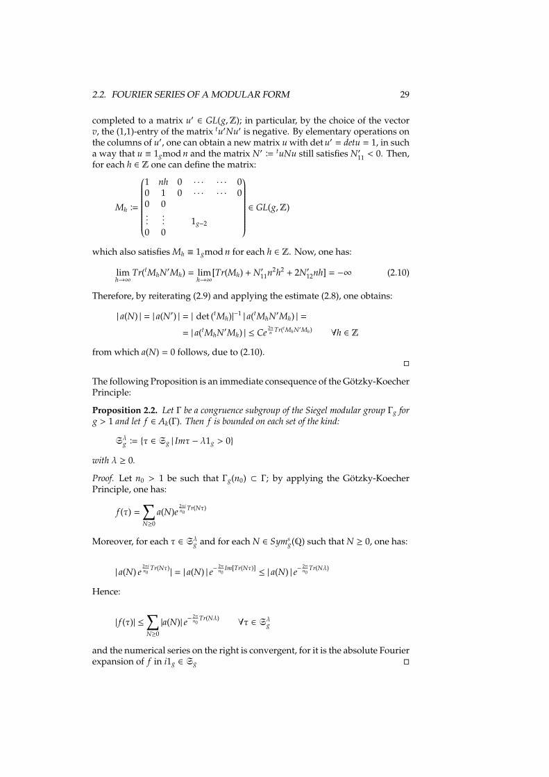
completed to a matrix u′ ∈ GL(g,Z); in particular, by the choice of the vectorv, the (1,1)-entry of the matrix tu′Nu′ is negative. By elementary operations onthe columns of u′, one can obtain a new matrix u with det u′ = detu = 1, in sucha way that u ≡ 1gmod n and the matrix N′ B tuNu still satisfies N′11 < 0. Then,for each h ∈ Z one can define the matrix:
Mh B
1 nh 0 · · · · · · 00 1 0 · · · · · · 00 0...
... 1g−20 0
∈ GL(g,Z)
which also satisfies Mh ≡ 1gmod n for each h ∈ Z. Now, one has:
limh→∞
Tr(tMhN′Mh) = limh→∞
[Tr(Mh) + N′11n2h2 + 2N′12nh] = −∞ (2.10)
Therefore, by reiterating (2.9) and applying the estimate (2.8), one obtains:
| a(N) | = | a(N′) | = | det (tMh)|−1| a(tMhN′Mh) | =
= | a(tMhN′Mh) | ≤ Ce2πn Tr(tMhN′Mh)
∀h ∈ Z
from which a(N) = 0 follows, due to (2.10).�
The following Proposition is an immediate consequence of the Gotzky-KoecherPrinciple:
Proposition 2.2. Let Γ be a congruence subgroup of the Siegel modular group Γg forg > 1 and let f ∈ Ak(Γ). Then f is bounded on each set of the kind:
Sλg B {τ ∈ Sg | Imτ − λ1g > 0}
with λ ≥ 0.
Proof. Let n0 > 1 be such that Γg(n0) ⊂ Γ; by applying the Gotzky-KoecherPrinciple, one has:
f (τ) =∑N≥0
a(N)e2πin0
Tr(Nτ)
Moreover, for each τ ∈ Sλg and for each N ∈ Symsg(Q) such that N ≥ 0, one has:
| a(N) e2πin0
Tr(Nτ)| = | a(N) | e−
2πn0
Im[Tr(Nτ)]≤ | a(N) | e−
2πn0
Tr(Nλ)
Hence:
| f (τ)| ≤∑N≥0
|a(N)| e−2πn0
Tr(Nλ)∀τ ∈ Sλg
and the numerical series on the right is convergent, for it is the absolute Fourierexpansion of f in i1g ∈ Sg �

30 CHAPTER 2. SIEGEL MODULAR FORMS
Corollary 2.1. Let Γ be a congruence subgroup of the Siegel modular group Γg forg > 1 and let f ∈ Ak(Γ). Then γ−1
|k f is bounded on Siegel’s fundamental domain Fgfor each γ ∈ Γg.
Proof. It follows from Proposizton 2.2 and Lemma 1.7. �
Corollary 2.1 shows that condition 3. in Definition 2.1 is a consequence of bothconditions 1. e 2. when g > 1.
Another important consequence of Gotzky-Koecher Principle is the following:
Corollary 2.2. Modular forms of negative weight vanish.
Proof. Let Γ be a congruence subgroup of the Siegel modular group Γg and letn0 > 0 be such that Γ(n0) ⊂ Γ.If f ∈ Ak(Γ) the function f is bounded on Siegel’s fundamental domain Fg (bydefinition when g = 1 and by Corollary 2.1 when g > 1).Moreover, if k < 0, by Lemma 1.7, the function τ 7→ |det Imτ|
k2 is bounded on
Fg. Then, there exists a constant C > 0 such that:
|det Imτ|k2 f (τ) ≤ C ∀τ ∈ Fg
The coefficients a(N) of the Fourier expansion of f satisfy thus for each y > 0:
| a(N) | e−2πn Tr(Ny)
≤
∫[0,n]K| f (x + iy)| |e
2πin Tr(Nx)
| dx ≤
≤ supx∈[0,n]K
f (x + iy) ≤ C |det Imτ|−k2
Then, letting y tend to zero, one obtains a(N) = 0 whenever N ≥ 0. �
Corollary 2.3. The ring of modular forms with respect to a congruence subgroup Γ isa positive graded ring A(Γ) =
⊕k≥0 A(Γ)k.
An important theorem generally guarantees the algebraic dependence ofsuitably many modular forms of given weight:
Theorem 2.3. Let Γ ⊂ Γg be a congruence subgroup. Then, for each k the complexvector space Ak(Γ) is finite-dimensional.
The existence of non-vanishing modular forms, however, is not a trivialquestion. Concerning the modularity with respect to the Siegel modular groupΓg, Eisenstein series are examples of non trivial modular forms of even weight.Other fundamental examples of modular forms with respect to the remarkablecongruence subgroups introduced in the Section 1.2 will be given in the follow-ing chapter by the Theta constants with characteristic. The next section will bedevoted, instead, to the introduction of a particular kind of modular forms.

2.3. CUSP FORMS 31
2.3 Cusp forms
Proposition 2.3. Let be 1 ≤ k ≤ g and {τn}n∈N ⊂ Sk a sequence such that:
τn =
(τ′ un
tun wn
)∀n ∈ N (2.11)
where τ′ ∈ Sk is a fixed point, {un}n∈N ⊂ Symk, g−k(C) is bounded, and {wn}n∈N is suchthat all the eigenvalues of Im(wn) tend to infinity. Then, the limit:
limn→∞
f (τn)
exists and is finite for each f ∈ A(Γg)
Proof. Let f ∈ A(Γg) and let:
f (τn) =∑
N∈Symsg(Z)
N≥0
a(N)e2πiTr(Nτn)∀n ∈ N
be its Fourier expansion. By hypothesis, the sequence {τn}n∈N is contained in aset on which the Fourier series of f uniformly converges. Since:
Tr(Nτ) Bg∑
i=1
Niiτii + 2∑
1≤i≤ j≤g
Ni jτi j
one has:
limn→∞
f (τn) =∑
N∈Symsk(Z)
N≥0
limn→∞
a(N)e2πiTr(Nτ) =∑
N′∈Symsr(Z)
N′≥0
a(N′ 00 0
)e2πiTr(N′τ′) (2.12)
Then the thesis follows, since τ′ ∈ Sk implies the convergence of the series onthe right. �
One has to observe that for a given couple g, k with 1 ≤ k ≤ g, and τ ∈ Sk fixed,there always exists a sequence {τn}n∈N ⊂ Sg of the kind in (2.11) with τ′ = τ.It will be convenient to denote by {ττn} any sequence of points in Sg satisfyingsuch a property.
For each couple g, k with 1 ≤ k ≤ g, Proposition 2.3 allows to define an operatoracting on modular forms by setting:
(Φg,k f )(τ) B limn→∞
f (ττn) ∀ f ∈ A(Γg) (2.13)
Proposition 2.4. The law (2.13) defines an operator Φg,k : A(Γg) → A(Γk) whichpreserves the weight.

32 CHAPTER 2. SIEGEL MODULAR FORMS
Proof. Let f ∈ Ah(Γg). It follows from (2.12) that for each τ ∈ Sk, (Φg,k f )(τ) doesnot depend on the choice of the sequence {ττn} ⊂ Sg; moreover, since the seriesin (2.12) is uniformly convergent on each compact, (2.13) defines a holomorphicfunction on Sk, which in case g = 1 is also bounded on the Siegel fundamentaldomain F1. Moreover, by setting:
γη B
aη 0 bη 00 1g−k 0 0cη 0 dη 00 0 0 1g−k
∈ Γg ∀η ∈ Γk
Since f ∈ Ah(Γg), the following transformation law holds for each η ∈ Γk, τ′ ∈ Skand λ > 0:
f(ητ′ 00 iλ1g−k
)= det (cητ′ + dη)
h f(τ′ 00 iλ1g−k
)Hence, when λ→∞, one has:
Φg,k f (ητ′) = det (cητ′ + dη)hΦg,k f (τ′) ∀ η ∈ Γk , ∀τ
′∈ Sk
and consequently Φg,k f ∈ Ah(Γk), which concludes the proof. �
Definition 2.4. The operator defined in (2.13) is called the Siegel operator.
As seen, the simplest way to describe the action of the Siegel operator is thefollowing:
Φ( f )(τ) = limλ→∞
f(τ 00 iλ
)∀ f ∈ A(Γk), ∀τ ∈ Sr (2.14)
The Siegel operator can be used to define the so-called cusp forms:
Definition 2.5. The elements of the complex vector space:
Sk(Γ) B { f ∈ Ak(Γ) |Φg,g−1(γ−1|k f ) = 0 ∀γ ∈ Γg}
are called cusp forms of weight k.
More generally, one can define the ideal of cusp forms with respect to a con-gruence subgroup Γ in A(Γ):
Definition 2.6. Let be Γ a congruence subgroup. The ideal S(Γ) B⊕
k≥0 Sk(Γ) ⊂ A(Γ)is called the ideal of the cusp forms with respect to Γ.
One has to remark that this definition characterizes the cusp forms withrespect to Γ as the modular forms which vanish on the boundary of the Satake’scompactification of AΓ (see Appendix B, (B.10)).
As well as for the rings of modular forms, one clearly has:
S(Γ′) ⊂ S(Γ) whenever Γ′ ⊂ Γ

2.3. CUSP FORMS 33
Example 2.4. The function ∆ introduced in Example 2.3 is a modular form of weight12. It is easily checked that:
limt→+∞
∆(it) = 0
Therefore, ∆ is a cusp form.

34 CHAPTER 2. SIEGEL MODULAR FORMS

Chapter 3
Theta constants
3.1 Characteristics
This section will be devoted to introduce the notion of characteristic, whichreveals itself to be involved in the parametrization of the so-called Theta con-stants.
Definition 3.1. A g-characteristic (or simply a characteristic, when no misunder-
standing is allowed) is a vector column[
m′
m′′
]with m′,m′′ ∈ Zg
2 .
Definition 3.2. Let m =
[m′
m′′
]be a characteristic. The function:
e(m) = (−1)tm′m′′ (3.1)
is called the parity of m. A characteristic m is called even if e(m) = 1 and odd ife(m) = −1.
Henceforward, the symbol C(g) will stand for the set of g-characteristics. Need-less to say, C(g) is isomorphic to Zg
2 × Zg2 as a ring; in particular, each g-
characteristic m satisfies m + m = 0.The symbols C(g)
e and C(g)o will respectively stand for the subset of even g-
characteristics and the subset of odd g-characteristics. Their cardinalities areeasily checked by introducing the notation:
mδ =
[m′ δ′
m′′ δ′′
]∈ C(g)
∀m =
[m′
m′′
]∈ C(g−1), ∀ δ =
[δ′
δ′′
]∈ C(1)
and by noting that, whenever m is even, mδ is even or odd, depending onwhether the 1-characteristic δ is respectively even or odd; on the other hand,whenever m is odd, mδ is even or odd, depending on whether δ is respectivelyodd or even. Since there are three even 1-characteristics[
00
] [10
] [01
]35

36 CHAPTER 3. THETA CONSTANTS
and only an odd one [11
]one thus has:
|C(g)e | = 3|C(g−1)
e | + |C(g−1)o |
|C(g)o | = |C
(g−1)e | + 3|C(g−1)
o |
Hence, |C(g)e | − |C
(g)o | = 2(|C(g−1)
e | − |C(g−1)o |). Then, one obtains by induction
|C(g)e |− |C
(g)o | = 2g, for |C(1)
e |− |C(1)o | = 2. Since |C(g)
e |+ |C(g)o | = 22g, one has, therefore:
|C(g)e | =
12 (22g + 2g) = 2g−1(2g + 1)
|C(g)o | =
12 (22g
− 2g) = 2g−1(2g− 1)
Thus, to sum up, there are 2g−1(2g + 1) even g-characteristics and 2g−1(2g− 1)
odd g-characteristics.
An action of the modular group Γg on the set C(g) can be defined by setting:
γ
[m′
m′′
]B
[(dγ −cγ−bγ aγ
) (m′
m′′
)+
(diag(cγtdγ)diag(aγtbγ)
)]mod2 (3.2)
It is easily verified by straightforward computations that:
γ(γ′m) = (γ · γ′)m, 1gm = m
as well as it is plainly checked that e(γm) = e(m) for each γ in Γg. Hence, onecan state:
Lemma 3.1. The law in (3.2) defines an action on C(g), which preserves the parity ofthe characteristics. This action is, in particular, not transitive.
More precisely, one has (cf. [I5] or [I3]):
Lemma 3.2. C(g) is decomposed into two orbits by the action in (3.2). These two orbitsconsist of the set of even characteristics and the set of odd characteristics.
The action defined in (3.2) is an affine transformation of C(g); the congruencesubgroup Γg(1, 2), in particular, acts linearly on C(g) by definition. Moreover:
Lemma 3.3. The action of the principal congruence subgroup Γg(2) on C(g) is trivial.

3.1. CHARACTERISTICS 37
Proof. Let γ ∈ Γg(2). Then, with reference to the notation introduced in (1.3),one has indeed:
γ
[m′
m′′
]=
[(12g + 2dM −2cM−2bM 12g + 2aM
) (m′
m′′
)]mod2 =
[m′
m′′
]�
Corollary 3.1. An action of Γg/Γg(2) � Sp(g,Z2) is defined on C(g).
The parity function can be used to classify remarkable k-plets of characteristicsaccording to the action introduced in (3.2). To pursue this purpose, a parity canbe also introduced for triplets:
e(m1,m2,m3) B e(m1)e(m2)e(m3)e(m1 + m2 + m3) (3.3)
Definition 3.3. A triplet (m1,m2,m3) is called azygetic if e(mi,m j,mh) = −1 andsyzygetic if e(mi,m j,mh) = 1
Concerning the parity of the sum of an odd sequence of g-characteristics, thefollowing formula holds (cf. [I7]):
e
2k+1∑i=1
=
2k+1∏i=1
e(mi)
∏
1<i< j≤2k+1
e(m1,mi,m j)
(3.4)
The parity is involved in characterizing the orbits of K-plets of g-characteristicsunder the action described in (3.2), as the following Proposition states (cf. [I5]):
Proposition 3.1. Let (m1, . . .mK) and (n1, . . .nK) be two ordered K-plets of g-characteristics.Then, there exists γ ∈ Γg such that γmi = ni for each i = 1, . . .n if and only if:
1. e(mi) = e(ni) for each i = 1, . . .K;
2. e(mi,m j,mk) = e(ni,n j,nk) for each 1 ≤ i < j < k ≤ K;
3. Whenever {m1, . . . ,m2k} ⊂ {m1, . . . ,mK} is such that m1 + · · ·m2k , 0, thenn1 + · · · n2k , 0;
Corollary 3.2. Let (m1, . . .mg) and (n1, . . .ng) be two different orderings of the setC(g)
e , such that for each l, r, s one has:
e(ml,mr,ms) = e(nl,nr,ns)
Then, there exists an element [γ] ∈ Γg/Γg(2) such that [γ]mi = ni for each i = 1, . . . g.

38 CHAPTER 3. THETA CONSTANTS
Proof. Let (m1, . . .mg) and (n1, . . .ng) be as in the hypothesis, and let {m1, . . . ,m2h} ⊂
{m1, . . . ,mg} be such that m1 + · · ·m2h = 0; then, by (3.4) one has:
1 = e(m2h) = e
2h−1∑i=1
mi
=
=∏
1<i< j≤2h−1
e(m1,mi,m j) =∏
1<i< j≤2h−1
e(n1,ni,n j) = e
2h−1∑i=1
ni
and, consequently, for each 1 ≤ l < r ≤ K one has:
e
nl,nr,2h−1∑i=1
ni
= e
nl + nr +
2h−1∑i=1
ni
= e(n1,nl,nr)∏
1<i< j≤2h−1
e(n1,ni,n j) =
= e(m1,ml,mr)∏
1<i< j≤2h−1
e(m1,mi,m j) = e
ml + mr +
2h−1∑i=1
mi
=
= e
ml,mr,2h−1∑i=1
mi
= e(ml,mr,m2k) = e(nl,nr,n2k)
Then∑2h−1
i=1 ni = n2h. Hence, whenever {m1, . . . ,m2h} ⊂ {m1, . . . ,mg} is such thatm1+· · ·m2h = 0, {n1, . . . ,n2h} ⊂ {n1, . . . ,ng} also verifies the condition n1+· · · n2h =0. Then the thesis follows from Proposition 3.1. �
The notion of azygeticity can be also given for K-plets of characteristics:
Definition 3.4. Let be{m1, . . . ,mK} a K-plet of characteristics. {m1, . . . ,mK} is calledazygetic if each subtriple {mi,m j,mh} is azygetic.
Since the case g = 2 will be relevant in ordrer to discuss the new resultsintroduced in this thesis, a focus on the main properties of k-plets of even 2-characteristics under the action in (3.2) will be needed. The next section willthus be centered around this technical feature.
3.2 k-plets of even 2-characteristics
A specific notation will be introduced here for subsets of even 2-characteristicsand conventionally used henceforward.The symbols C1 B C(2)
e and C1 B C(2)o will stand respectively for the set of even
2-characteristics and the set of odd 2-characteristics, so that C(2) = C1 ∪ C1 with|C1| = 10 and |C1| = 6.
The symbols C e C will denote respectively the parts of C1 and the parts of C1.More in general, Ck ∈ C will stand for the set of k-plets of even 2-characteristicsand Ck ∈ C for the set of k-plets of odd 2-characteristics.
For each subset M ⊂ C1 its complementary set C1 −M in C1 will be denotedas Mc. The so called symmetric difference will be represented by the classicnotation:

3.2. K-PLETS OF EVEN 2-CHARACTERISTICS 39
Mi MM j B (Mi ∪M j) − (Mi ∩M j) ∈ C ∀Mi,M j ∈ C
Therefore, for each couple Mi, M j ⊂ C1, C1 can be written as a disjoint union ofsets:
C1 =(Mi
c∩M j
c)∪
(Mi ∩M j
)∩
(Mi MM j
)(3.5)
The chief aim of this section is to point out some combinatorial features relatedto remarkable subsets of Ck, which will be needed in the last chapter; thesesubset arise as orbits under the action of Γ2/Γ2(2).In fact, when g = 2, by Corollary 3.1 and Lemma 3.2 the group Γ2/Γ2(2) bothacts on C1 and C1. By focusing on the action on C1 one note that the grouphomomorphism naturally defined by:
ψP : Γ2/Γ2(2) 7→ S6 (3.6)
is injective, for the identity in Γ2/Γ2(2) is the only element which fix all thesix odd 2-characteristics. Moreover, Γ2/Γ2(2) � Sp(2,Z2) and S6 have the sameorder, hence the homomorphism (3.6) is also surjective. Then:
Γ2/Γ2(2) � S6 (3.7)
An action of this group is naturally defined on each Ck, by the one definedon C1. While the action on C2 is transitive, each Ck for k > 2 turns out to bedecomposed into orbits, which can be described using Corollary 3.2. Seekinga notation imported from [vGvS], one observes that the set C3 is, in particular,decomposed into two orbits C−3 and C+
3 , which consist respectively of azygeticand syzygetic triplets:
C−3 = { {m1,m2,m3} ∈ C3 | m1 + m2 + m3 ∈ C1}
C+3 = { {m1,m2,m3} ∈ C3 | m1 + m2 + m3 ∈ C1}
with |C−3 | = |C+3 | = 60.
The set C4 decomposes into three orbits C+4 , C∗4 and C−4 , where, in particular:
C−4 = { {m1, . . . ,m4} ∈ C4 | {mi,m j,mk} ∈ C−3 ∀{mi,m j,mk} ⊂ {m1, . . . ,m4} }
C+4 = { {m1, . . . ,m4} ∈ C4 | {mi,m j,mk} ∈ C+
3 ∀{mi,m j,mk} ⊂ {m1, . . . ,m4} }
40 CHAPTER 3. THETA CONSTANTS
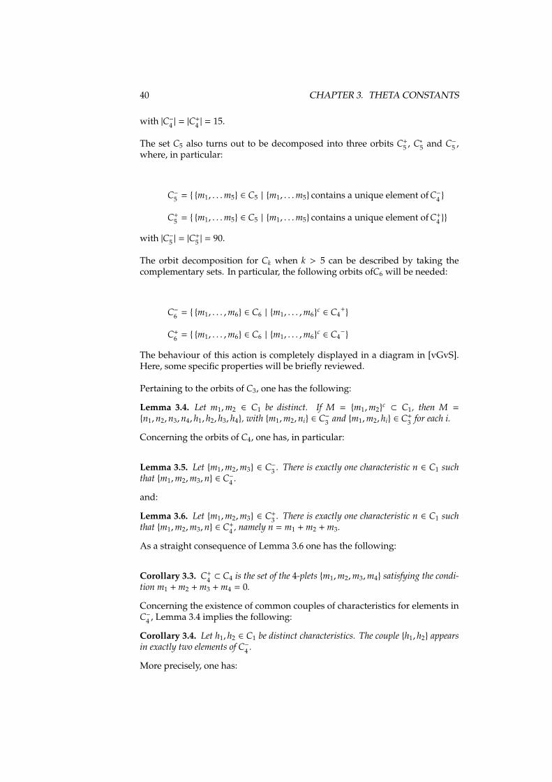
with |C−4 | = |C+4 | = 15.
The set C5 also turns out to be decomposed into three orbits C+5 , C∗5 and C−5 ,
where, in particular:
C−5 = { {m1, . . .m5} ∈ C5 | {m1, . . .m5} contains a unique element of C−4 }
C+5 = { {m1, . . .m5} ∈ C5 | {m1, . . .m5} contains a unique element of C+
4 }}
with |C−5 | = |C+5 | = 90.
The orbit decomposition for Ck when k > 5 can be described by taking thecomplementary sets. In particular, the following orbits ofC6 will be needed:
C−6 = { {m1, . . . ,m6} ∈ C6 | {m1, . . . ,m6}c∈ C4
+}
C+6 = { {m1, . . . ,m6} ∈ C6 | {m1, . . . ,m6}
c∈ C4
−}
The behaviour of this action is completely displayed in a diagram in [vGvS].Here, some specific properties will be briefly reviewed.
Pertaining to the orbits of C3, one has the following:
Lemma 3.4. Let m1,m2 ∈ C1 be distinct. If M = {m1,m2}c⊂ C1, then M =
{n1,n2,n3,n4, h1, h2, h3, h4}, with {m1,m2,ni} ∈ C−3 and {m1,m2, hi} ∈ C+3 for each i.
Concerning the orbits of C4, one has, in particular:
Lemma 3.5. Let {m1,m2,m3} ∈ C−3 . There is exactly one characteristic n ∈ C1 suchthat {m1,m2,m3,n} ∈ C−4 .
and:
Lemma 3.6. Let {m1,m2,m3} ∈ C+3 . There is exactly one characteristic n ∈ C1 such
that {m1,m2,m3,n} ∈ C+4 , namely n = m1 + m2 + m3.
As a straight consequence of Lemma 3.6 one has the following:
Corollary 3.3. C+4 ⊂ C4 is the set of the 4-plets {m1,m2,m3,m4} satisfying the condi-
tion m1 + m2 + m3 + m4 = 0.
Concerning the existence of common couples of characteristics for elements inC−4 , Lemma 3.4 implies the following:
Corollary 3.4. Let h1, h2 ∈ C1 be distinct characteristics. The couple {h1, h2} appearsin exactly two elements of C−4 .
More precisely, one has:

3.2. K-PLETS OF EVEN 2-CHARACTERISTICS 41
Lemma 3.7. Let {m1,m2, h, k}, {m3,m4, h, k} ∈ C−4 be distinct 4-plets. Then:
{m1,m2,m3,m4} ∈ C−4
Lemma 3.8. Let {m1,m2,m3,n}, {m4,m5,m6,n} ∈ C−4 be such that mi,n are all distinct.Then:
{m7,m8,m9,n} ∈ C−4
where {m7,m8,m9} = {m1,m2,m3,m4,m5,m6,n}c
The following property holds for C−5 :
Proposition 3.2. If M < C−5 , M does not contain any element of C−4 .
For the orbits of C6, one has:
Proposition 3.3. M ∈ C−6 if and only if M contains exactly six elements of C−5 .
Moreover, Corollary 3.3 implies the following:
Corollary 3.5. M ∈ C−6 if and only if∑
m∈M m = 0.
Then it follows that:
Lemma 3.9. M ∈ C−6 if and only if M does not contain any element of C+4 .
Proof. A 4-plets {m1,m2,m3,m4} ∈ C−4 can not belong to an element of C−6 ,for
∑4i=1 mi = 0. �
By taking the complementary sets, one obtains:
Lemma 3.10. M ∈ C+6 if and only if M does not contain any element of C−4 .
For elements M1,M2 belonging both to C+4 and C−6 Corollaries 3.3 and 3.5 point
out immediately a property satisfied by their symmetric difference:
0 =∑
m∈M1
m +∑
m∈M2
m =∑
m∈M1MM2
m (3.8)
The behaviour of the symmetric difference of elements of C−4 and C+6 can be
described more precisely, using the results gathered throughout this section.
Proposition 3.4. Let M1,M2 ∈ C−4 . Then M1 ∩M2 , ∅ and:
1) M1 MM2 ∈ C+6 i f |M1 ∩M2| = 1
2) M1 MM2 ∈ C−4 i f |M1 ∩M2| = 2
3) M1 = M2 i f |M1 ∩M2| > 2

42 CHAPTER 3. THETA CONSTANTS
Proof. Lemma 3.10 implies M2 1 Mc1, hence M1 ∩M2 , ∅. The possible cases
are thus to be checked:
1) If M1∩M2 = {n}, one can set M1 = {m1,m2,m3,n} and M2 = {m4,m5,m6,n}.Then, by Lemma 3.8, M1 MM2 = {m1,m2,m3,m4,m5,m6} = {m7,m8,m9,n}c ∈ C+
6 .
2) If M1 ∩M2 = {h, k}, one can set M1 = {m1,m2, h, k} and M2 = {m3,m4, h, k}.Then, by Lemma 3.7, M1 MM2 = {m1,m2,m3,m4} ∈ C−4 .
3) As a straight consequence of Lemma 3.5, if M1 and M2 share at least 3common characteristics, they must be the same element of C−4 �
Proposition 3.5. Let M1,M2 ∈ C+6 . Then, the only possible cases are:
1) M1 MM2 ∈ C+6 i f |M1 ∩M2| = 3
2) M1 MM2 ∈ C−4 i f |M1 ∩M2| = 4
3) M1 = M2 i f |M1 ∩M2| > 4
Proof. Since |C1| = 10, obviously |M1 ∩M2| ≥ 2.Moreover, the relation 12 = |M1|+ |M2| = |M1 ∪M2|+ |M1 ∩M2|, combined with(3.5), implies:
|M1 ∩M2| − |Mc1 ∩Mc
2| = 2 (3.9)
Therefore |M1 ∩M2| > 2, because Mc1 ∩Mc
2 , ∅ by Proposition 3.4.
Now, the remaining cases are to be checked.
1) If M1 ∩ M2 = {h, k, l}, one can set M1 = {m1,m2,m3, h, k, l} and M2 ={m4,m5,m6, h, k, l}. Then, Mc
1 = {m4,m5,m6,n} ∈ C−4 and Mc2 = {m1,m2,m3,n} ∈
C−4 , where n , mi, h, k, l. Therefore, by Lemma 3.8, M1 MM2 = {h, k, l,n}c ∈ C+6 .
2) If M1 ∩ M2 = {n, h, k, l}, one can set M1 = {m1,m2,n, h, k, l} and M2 ={m3,m4,n, h, k, l}. Then, Mc
1 = {m3,m4, i, j} ∈ C−4 and Mc2 = {m1,m2, i, j} ∈ C−4 ,
where i, j , mi, ,n, h, k, l. Hence, by Lemma 3.7, M1 M M2 = {m1,m2,m3,m4} ∈
C−4 .
3) If |M1 ∩M2| > 4, then (3.9) implies |Mc1 ∩Mc
2| > 2; therefore, Mc1 = Mc
2 byProposition 3.4, and consequently M1 = M2. �
Proposition 3.6. Let M1 ∈ C+6 and M2 ∈ C−4 . If Mc
1 , M2 the only possible cases are:
1) M1 MM2 ∈ C−4 i f |M1 ∩M2| = 3
2) M1 MM2 ∈ C+6 i f |M1 ∩M2| = 2
Proof. Obviously |M1 ∩M2| ≤ 4; moreover, Lemma 3.10 implies that M2 1 M1,hence |M1 ∩M2| ≤ 3. If Mc
1 , M2, Lemma 3.5 implies |Mc1 ∩M2| < 3 and conse-
quently |M1 ∩M2| > 1. Therefore, the only cases to be checked, when Mc1 , M2,

3.3. THETA CONSTANTS 43
are the cases 1) and 2):
1) If M1 ∩ M2 = {h, k, l}, one can set M1 = {m1,m2,m3, h, k, l} and M2 ={m4, h, k, l}. Then Mc
2 = {m1,m2,m3, r, s, t} ∈ C+6 with r, s, t , mi, h, k, l, and by
Proposition 3.5 (case 1) one has:
M1 MM2 = {m1,m2,m3,m4} = {h, k, l, r, s, t}c = (M1 MMc2)c∈ C−4
2) If M1 ∩ M2 = {h, k}, one can set M1 = {m1,m2,m3,m4, h, k} and M2 ={m5,m6, h, k}. Then Mc
1 = {m5,m6, i, j} ∈ C−4 with i, j , mi, h, k, and by Proposition3.4 (case 2) one has:
M1 MM2 = {m1,m2,m3,m4,m5,m6} = {i, j, h, k}c = (Mc1 MM2)c
∈ C+6
�
3.3 Theta constants
Theta constants play an essential role in the construction of several modularforms. The aim of this section is to introduce these remarkable functions as wellas to outline their main basic properties. The main references for this sectionwill be Igusa’s classical works [I5], [I3] and [I4], Freitag’s book [F], Farkas andKra’s book [FK] and Mumford’s lectures [Mf].
Definition 3.5. For each m = (m′,m′′) ∈ Zg×Zg, the function θm : Sg × C
g→ C,
defined by:
θm(τ, z) B∑n∈Zg
exp{
t(n +
m′
2
)τ(n +
m′
2
)+ 2t
(n +
m′
2
) (z +
m′′
2
)}(3.10)
is called Riemann Theta function with characteristic m = (m′,m′′).
The series in (3.10) is easily seen to be absolutely convergent and uniformlyconvergent on each compact of Sg ×C
g; therefore, for each m it defines a holo-morphic function. One can note that in the case g = 1 the series for m = 0 is theclassical Jacobi Theta function.
By setting:
τ B (τ 1g) ∈ Symg, 2g(C) ∀τ ∈ Sg (3.11)
is plainly verified that for each m = (m′,m′′), n = (n′,n′′) ∈ Zg× Zg the Theta
function with characteristic m satisfies the equation 1
θm(τ, z + τn) = (−1)tm′n′′−tm′′n′exp
{2t
(−
tn′z −12
tnτn′)}θm(τ, z) (3.12)
1One proves that any other holomorphic function θ : Cn→ Cwhich is solution of (3.12) differs
from the Theta function with characteristic by a multiplicative factor; for each τ ∈ Sg fixed, thefunction z 7→ θm(τ, z) is, therefore, characterized as an analytic function on Cn, by being solutionof the equation (3.12).

44 CHAPTER 3. THETA CONSTANTS
As proved through term by term differentiation, the Theta function with char-acteristic also satisfies the heat equation: 2.
g∑j,k=1
σ jk∂θm
∂z jzk= 2πi
g∑j,k=1
σ jk∂θm
∂τ jk(3.13)
With reference to the actions of Γg described in (1.10) and (3.2) , if n = γmwith γ ∈ Γg, it easily turns out that:
θn(γτ, t(cγτ+dγ)−1z) = K(m, γ, τ) exp{2(−
12
tz(cγτ + dγ)−1cγz)}θm(τ, z) (3.14)
where K : Z2g× Γg × Sg → C is a non-vanishing function, which does not
depend on the variable z.
The g-characteristics parametrize distinct Theta functions. The definition(3.10) implies, indeed:
θm+2n(τ, z) = (−1)tm′n′′θm(τ, z)
for each m = (m′,m′′), n = (n′,n′′) ∈ Zg× Zg. Hence, in order to study Theta
functions one can focus on the only ones which are related to g-characteristics.
Definition 3.6. For each characteristic m the holomorphic function θm : Sg → C,defined by:
θm(τ) B θm(τ, 0) (3.15)
is called Theta constant with characteristic m.
From (3.10), in particular, it follows that:
θm(τ,−z) = e(m)θm(τ, z) (3.16)
where e(m) is the parity of the characteristic m introduced in (3.1) 3 By (3.16),Theta constants related to odd characteristics vanish. On the converse, oneeasily notes that limλ→∞ θ0(iλ1g) = 1; hence, the Theta constant θ0, relatedto the null characteristic, does not vanish. Lemma 3.2 and the non-vanishingproperty of the function K imply that each Theta constant θm, related to an evencharacteristic m, does not vanish.
In order to determine an explicit expression for the function K, the followingdifferential equation, derived form (3.13) for even characteristics, can be used:
∑1≤ j,k≤g
σ jk∂ log Kτ jk
=12
∑1≤ j,k≤g
σ jkµ jk
2One also proves that as a holomorphic function θm : Sg × Cg→ C, the Theta function is
characterized by being solution of (3.12) and (3.13)3The formula (3.16) justifies the classical choice to define this function a parity.

3.3. THETA CONSTANTS 45
As it can be shown, it implies:
K(m, γ, τ) = C(m, γ) det (cγτ + dγ)12
where C is a function which does not depend on τ. In particular, one has toobserve that, albeit the root det (cγτ + dγ)
12 is not unique, it is well defined as an
analytic function on Sg.Now, for each n = (n′,n′′) ∈ C(g) e τ = (τ 1g) as in (3.11), one has:
θm
(τ, z +
12τn
)= exp
{2[−
18
tn′τn′ −12
tn′(z +
12
(m′′ + n′′))]}
θm+n(τ, z)
Then, by selecting the branch of det (cγτ + dγ)12 whose sign turns to be positive
when Reτ = 0, and applying (3.14), one has for each γ ∈ Γg:
θγ0(γτ, t(cγτ+dγ)−1z) = C(m, γ) det (cγτ + dγ)12 exp
{2(1
2tz(cγτ + dγ)−1cγ
)}θ0(τ, z)
Operating for each even characteristic m the substitution z 7→ z + 12 τm, the
multiplicative factor of C, depending only on m, can be explicited; hence one issupplied with the following transformation law for the Theta function:
θγm(γτ , t(cγτ + dγ)−1z) = κ(γ)eπi{ 12
tz [(cγτ+dγ)−1cγ] z+2φm(γ)}det(cγτ + dγ)12θm(τ, z)
∀γ ∈ Γg, ∀m ∈ C(g), ∀τ ∈ Sg, ∀z ∈ Cg
(3.17)
where:
φm(γ) = −18
(tm′tbγdγm′ + tm′′taγcγm′′ − 2tm′tbγcγm′′)+
−14
tdiag(aγtbγ)(dγm′ − cγm′′)(3.18)
and det (cγτ + dγ)12 is the root, which has been chosen in the described way.
In particular, the function:
Φ(m, γ, τ, z) B κ(γ)eπi{ 12
tz [(cγτ+dγ)−1cγ] z+2φm(γ)}
is such that Φ|z=0 does not depend on τ. For this reason the functions θm definedin (3.15) are called Theta constants; the transformation law in (3.17) becomesfor Theta constants:
θγm(γτ) = κ(γ)χm(γ)det(cγτ + dγ)12θm(τ)
∀γ ∈ Γg, ∀m ∈ C(g), ∀τ ∈ Sg,(3.19)

46 CHAPTER 3. THETA CONSTANTS
where:
χm(γ) B Φ(m, γ, τ, 0) = e2πiφm(γ) (3.20)
Concerning the function κ, an important property can be stated:
Proposition 3.7. κ2 is a character of Γg(1, 2).
Proof. Since χ0 = 1 for the null characteristic m = 0 (by definition in (3.20)and (3.18)), by applying (3.19) to the Theta constant θ0 related to the nullcharacteristic, one obtains:
θ2γ0(γτ) = κ2(γ)det(cγτ + dγ)θ2
0(τ)
Since Γg(1, 2) acts linearly, γ0 = 0 whenever γ ∈ Γg(1, 2); then:
det(cγτ + dγ)−1θ20(γτ) = κ2(γ)θ2
0(τ) ∀γ ∈ Γg(1, 2)
Hence, with reference to the action introduced in (2.1), one has:
γ−1|1θ
20 = κ2(γ)θ2
0 ∀γ ∈ Γg(1, 2)
and consequently:
κ2(γγ′)θ20(τ) = κ2(γ)κ2(γ′)θ2
0(τ) ∀γ, γ′ ∈ Γg(1, 2)
Then κ2(γγ′) = κ2(γ)κ2(γ′) and κ2(11g) = 1, for θ0 does not vanish; hence thethesis follows. �
The following Lemma provides an expression for the function κ for specialelements of Γg:
Lemma 3.11. Let:
γ =
(aγ bγ0 dγ
)∈ Γg
Then:
κ2(γ) = κ2(tγ−1) = det (dγ)
Proof. The proof of the whole statement can be found in [I4]. Here it will beonly shown that κ2(γ) = det (dγ).Since χ0 = 1, the transformation law (3.19) implies in particular:
θ2γ0(γτ) = κ2(γ)det (dγ)θ2
0(τ)
∀γ =
(aγ bγ0 dγ
)∈ Γg
As θ2γ0(γτ) = θ2
0(τ), one has κ2(γ) = det (dγ). �

3.3. THETA CONSTANTS 47
As a consequence of this Lemma, one obtains a description for the possiblevalues of the function κ:
Proposition 3.8. For each γ ∈ Γ, κ(γ) is an eight root of the unity.
Proof. By definition in (3.20) and (3.18), one clearly has χ8m = 1. Then (3.19)
implies:
det(cγτ + dγ)−4θ8γm(γτ) = κ8(γ)θ8
m(τ)
∀γ ∈ Γg, ∀m ∈ C(g)
Again with reference to the action introduced in (2.1), one has:
γ−1|4θ
8γm = κ8(γ)θ8
m ∀γ ∈ Γg, ∀m ∈ C(g)
Hence:
κ8(γγ′)θ8m(τ) = κ8(γ)κ8(γ′)θ8
m(τ) ∀γ, γ′ ∈ Γg ∀m ∈ C(g)
Then, κ8 is a character of Γg. Moreover, by Lemma 3.11, one has:
κ4(γ) = 1 κ4(tγ−1) = 1
whenever γ ∈ Γg is such that cγ = 0; since by Corollary 1.1 these elementsgenerates Γg, one has:
κ8(γ) = 1 ∀γ ∈ Γg (3.21)
�
An explicit expression for κ4, which can be found in [I3], is recalled in thefollowing statement:
Proposition 3.9. For each γ ∈ Γg the following expression holds:
κ(γ)4 = eπTr(tbγcγ)i (3.22)
A simple explicit expression for κ2 on suitable congruence subgroups canbe also found, using Proposition 3.7:
Proposition 3.10. For each γ ∈ Γg(2) the following expression holds:
κ(γ)2 = eπ2 Tr(aγ−1g)i (3.23)
Proof. Let γ, γ′ ∈ Γg(2). With reference to the notation in (1.3) one has:
aγγ′ = 1g + 2(aM + aM′ ) + 4aMaM′ + 4bMcM′
Therefore, by setting:

48 CHAPTER 3. THETA CONSTANTS
g(γ) B eπ2 Tr(aγ−1g)i
one has:
g(γγ′) = eπ2 2Tr(aM+aM′ )i = e
π2 2TraMie
π2 2TraM′ )i =
= eπ2 Tr(aγ−1g)ie
π2 Tr(aγ′−1g)i = g(γ)g(γ′)
Consequently, the function g is a character of Γg(2). However, κ2 is also acharacter of Γg(2), by Proposition 3.7. Then, by using Lemma 3.11, it can bedirectly checked that g(γ) = κ2(γ) and g(tγ−1) = κ2(tγ−1), whenever γ is suchthat cγ = 0; since by Proposition 1.4 the generators of Γg(2) are such elements,the characters g and κ2 coincide on Γg(2). �
Thanks to (3.23) one has, in particular:
k2(γ) = 1 ∀γ ∈ Γ(4, 8) (3.24)
and
κ2(−12g) =
1 if g is even
−1 if g is odd(3.25)
The formula (3.25) implies, in particular, that the function κ2 is well definedon the quotient group Γg(2)/{±12g} if g is even. Then, Proposition 3.7 implies:
Corollary 3.6. When g is even, κ2 is a character of Γg(2)/{±12g}.
Moreover, one has:
Corollary 3.7. When g is even, κ2 is a character of the group Γg(2, 4)/{±Γ(4, 8)}.
Proof. When g is even, Corollary 3.6 implies, in particular, that κ2 is a characterof Γg(2, 4)/{±12g}; hence the thesis follows, since κ2 is well defined on thequotient Γg(2, 4)/{±Γ(4, 8)} due to (3.24). �
Concerning the function χm introduced in (3.20), a straightforward compu-tation allows to verify a basic properties:
Lemma 3.12.
χm(−12g) =
1 if m is even
−1 if m is odd

3.3. THETA CONSTANTS 49
Moreover, one has:
Lemma 3.13. Let be Ai j,Bi j,Ci j ∈ Γg(2, 4) as in Proposition 1.4. Then, for each char-
acteristic m =
[m′
m′′
]one has:
χm(Ai j) = (−1)m′i m′′
j
χm(Bi j) = (−1)m′i m′
j
χm(Ci j) = (−1)m′′′i m′′j
χm(B2ii) = (−1)m′2i (i < j)
χm(C2ii) = (−1)m′′2i (i < j)
where m′i and m′′i denote respectively the i-th coordinate of m′ and the i-th coordinateof m′′.
Proof. By applying (3.18) to the generic element in Γg(2, 4), one finds:
χm(γ) = eπ2
tm1(−bγm′+aγm′′−m′′)ie−π4 (tm′ tbγdγm′+tm′′taγcγm′′)i
∀γ ∈ Γg(2, 4)(3.26)
thanks to which the values in the statement can be computed. �
By Corollary 1.2, using Lemmas 3.12 and 3.13, the following statements can bestraightly proved:
Lemma 3.14. χ2m(γ) = 1 for each γ ∈ Γg(2, 4)
Lemma 3.15. For each characetristic m ∈ C(g), χm is a character of Γg(2, 4).
Lemma 3.16. χm(γ) = 1 for each γ ∈ Γg(4, 8).
By Lemmas 3.15 and 3.16 one has, in particular:
Corollary 3.8. For each characteristic m ∈ C(g), the function χm is well defined on thequotient group:
χm : Γg(2, 4)/Γg(4, 8) −→ C∗
Moreover χm is a character of Γg(2, 4)/Γg(4, 8) 4.
Corollary 3.8 and Lemma 3.12 imply, in particular:
4Likewise, one can observe that Lemma 3.14, allows to define χ2m on the quotient group
Γg(2)/Γg(2, 4), hence χ2m is a character of this group. (cf. [SM2])

50 CHAPTER 3. THETA CONSTANTS
Corollary 3.9. Let m,n ∈ C(g). If m and n are both even or odd, the function χmχn iswell defined on the quotient group:
χmχn : Γg(2, 4)/{±Γg(4, 8)} −→ C∗
and is a character of Γg(2, 4)/{±Γg(4, 8)} 5.
In general, one can prove the following:
Proposition 3.11. The set {χm}, parametrized by the even characteristics m, is a setof generators for thel group Γg(2, 4)/{±Γg(4, 8)}.
Proof. A proof can be found in [SM2]. �
As a consequence of (3.19), the action of the modular group Γg can be defined oncouples of characters χmχn. In fact, if one defines for each γ ∈ Γg the function:
γ · χm(η) B χm(γηγ−1) (3.27)
the following statement holds:
Proposition 3.12. The law (3.27) defines an action of the modular group Γg on theproducts χmχn satisfying the property:
γ(χmχn) = (γ · χm)(γ · χn) = χγ−1mχγ−1n (3.28)
Proof. With reference to the action introduced in (2.1), (3.18) and (3.19) implyfor each γ ∈ Γ:
γ−1|1θmθn = κ2(γ)e2πi(φγ−1m(γ)+φγ−1n(γ))θγ−1mθγ−1n (3.29)
Now, let be m,n both even. Then (3.29) implies:
κ2(γ)κ2(γ−1)e2πi(φγ−1m(γ)+φγ−1n(γ))e2πi(φγm(γ−1)+φγn(γ−1)) = 1 (3.30)
Hence, for each γ ∈ Γg and η ∈ Γg(2, 4):
((γηγ−1)−1|1θmθn)(τ) = κ2(γηγ−1)2χm(γηγ−1)χn(γηγ−1)θm(τ)θn(τ) (3.31)
But since
γ−1|1θmθn = κ2(γ)χmχnθγ−1mθγ−1n ∀γ ∈ Γg(2, 4) (3.32)
one also has by (3.30):
((γηγ−1)−1|1θmθn)(τ) = κ2(η)χγ−1m(η)χγ−1n(η)θm(τ)θn(τ) (3.33)
5More in general χmχn is proved to be a character of Γg(2)/{±1g}.

3.3. THETA CONSTANTS 51
Then the thesis follows from (3.31) and (3.33), for (3.23) implies:
κ2(γηγ−1) = κ2(η) ∀γ ∈ Γg, ∀η ∈ Γg(2, 4)
Concerning the other cases, since for each odd characteristic n the holomorphicmaps:
grad0zθn B gradzθn|z=0 =
(∂∂z1
θn|z=0, . . . ,∂∂zg
θn|z=0
)satisfy the following transformation law:
grad0zθn(γτ) = det (cγτ + dγ)
12 (cγτ + dγ) · grad0
zθn(τ)
∀γ ∈ Γg(4, 8), ∀τ ∈ Sg
(3.34)
one can likewise use the same argument on θmgrad0zθn and on grad0
zθmgrad0zθn
to prove the statement respectively when m is even and n is odd and when bothm and n are odd. �
The transformation law in (3.34) means, in particular, that gradients of oddTheta functions can be regarded as modular forms with respect to Γg(4, 8) underthe representation 6:
T0(A) B det (A)1/2A (3.35)
Such a behaviour allows to define the map, on which the thesis will focus inthe next chapter.
As a consequence of the Proposition 3.12 Γg acts on even sequences of char-acters χm.
Thanks to some of the results gathered here, the modular property of theTheta constants can be discussed:
Proposition 3.13. The product of two Theta constants θmθn is a modular form ofweight 1 with respect to Γg(4, 8).
Proof. First of all, by Lemma 3.3, the law (3.19) turns out to be:
θm(γτ) = κ(γ)χm(γ) det (cγτ + dγ)12θm(τ)
∀γ ∈ Γg(2), ∀m ∈ C(g), ∀τ ∈ Sg,(3.36)
Then, by applying (3.24) and Lemma 3.16, one is supplied with the followingtransformation law:
θmθn(γτ) = det (cγτ + dγ)θmθn(τ)
∀γ ∈ Γg(4, 8), ∀m ∈ Cg, ∀τ ∈ Sg,(3.37)
which proves the thesis. �
6The classical modular forms of weight k, which are the only ones discussed in this work, areindeed modular forms under the representation T(A) B det (A)k

52 CHAPTER 3. THETA CONSTANTS
A useful criterion of modularity with respect to Γg(2, 4) can be more gener-ally stated for products of an even sequence of Theta constants:
Proposition 3.14. Let M = (m1, . . . ,m2k) be a sequence of even characteristics. Theproductθm1 · · ·θm2k is a modular form with respect to Γg(2, 4) if and only if the followingcondition is verified:
M tM ≡ k(0 11 0
)mod 2 (3.38)
Proof. Let M = (m1, . . . ,m2k) be a sequence of even characteristics; one can set:
mh =
[m′hm′′h
]for each characteristic mh appearing in the sequence M, and m′h,(i) and m′′h,(i)respectively for the i-th coordinate of m′h and m′′h .Now, by (3.36) and (3.23), if k is even, θm1 · · ·θm2k is a modular form withrespect to Γg(2, 4) if and only if the character χM B χm1 · · ·χm2k is trivial onΓg(2, 4). Due to Corollary 1.2, this is true if and only if the elements Ai j (for i, j ,g),Bi j,Ci j (for i < j),B2
ii,C2ii belong to the kernel KerχM. Then, Lemma 3.13
translates this criterion into conditions for the sequence M:
a)∑k
h=1(m′h,(i))2 = 0 ∀ i ( χM(B2
ii) = 1 )
b)∑k
h=1(m′′h,(i))2 = 0 ∀ i ( χM(C2
ii) = 1 )
c)∑k
h=1 m′h,(i)m′
h,( j) = 0 ∀ i < j ( χM(Bi j) = 1 )
d)∑k
h=1 m′′h,(i)m′′
h,( j) = 0 ∀ i < j ( χM(Ci j) = 1 )
e)∑k
h=1 m′h,(i)m′′
h,( j) = 0 ∀ i, j , g ( χM(Ai j) = 1 )
Therefore, for k even, one has the criterion:
M tM ≡(0 00 0
)mod 2
Now, if k is odd, (3.36) and (3.23) imply that θm1 · · ·θm2k is a modular form withrespect to Γg(2, 4) if and only if κ2χM is trivial on Γg(2, 4). Using the definitionof these elements (see Proposition 1.4), one can apply (3.23) and verify that theAii are the only elements on which the function κ2 assumes the value −1 . Thenconditions a) b) c) d) keep unchanged, while condition e) is substituted by atwofold condition:
e′)∑k
h=1 m′h,(i)m′′
h,( j) = 0 ∀ i , j ( κ2χM(Ai j) = 1 )
e′′)∑k
h=1 m′h,(i)m′′
h,(i) = 1 ∀ i ( κ2χM(Ai j) = 1 )

3.3. THETA CONSTANTS 53
Hence, for k odd one has the criterion:
M tM ≡(0 11 0
)mod 2
which concludes the proof. �
Concerning the product of all the non-vanishing Theta constants:
χ(g) B∏
m even
θm (3.39)
one knows by Proposition 3.13 that for g ≥ 2 χ(g) is a modular form of weight2g−2(2g + 1) with respect to Γg(4, 8). However, for each γ ∈ Γg one has by (3.17):
∏m even
θm(γτ) =∏
m even
θγm(γτ) =
=
κ2g−1(2g+1)(γ)∏
m even
χm(γ)
det (cγτ + dγ)2g−2(2g+1)∏
m even
θm(τ)
and the character appearing is trivial whenever g ≥ 3. Therefore, one has thefollowing:
Proposition 3.15. When g ≥ 3, χ(g) is a modular form of weight 2g−2(2g + 1) withrespect to Γg.
The case g = 2 is a special one; the product
χ5 B χ(2) B∏m∈C1
θm (3.40)
satisfying the transformation law:
χ5(γτ) = κ2(γ)∏
m∈C1χm(γ) det (cγτ + dγ)5χ5(τ)
∀γ ∈ Γg
(3.41)
is not a modular form with respect to Γ2, since the character appearing is nottrivial. However, the function:
χ10 B χ25 =
∏m∈C1
θm
2
(3.42)
is a modular form of weight 10 with respect to Γ2.
Other remarkable modular forms with respect to suitable congruence sub-groups can be built by the following notable functions:

54 CHAPTER 3. THETA CONSTANTS
Definition 3.7. For each m′ ∈ Zg2 the holomorphic function Θm′ : Sg × C
g→ C,
defined by:
Θm′ (τ, z) B θ[m′0
](2τ, 2z) (3.43)
is called a second order Theta function.
In particular,, one has the following:
Definition 3.8. For each m′ ∈ Zg2 the holomorphic function:
Θm′ (τ) B θ[m′0
](2τ, 0) = θ[m′0
](2τ) (3.44)
is named second order Theta constant.
A transformation law for second order Theta constants can be easily derivedby focusing on the congruence subgroup Γg,0(2) introduced in (1.5).For each γ ∈ Γg one can define:
γ B
(aγ 2bγ12 cγ dγ
)∈ Sp(g,Q)
Then, by definition in (1.10), one has 2γτ = γ2τ for each τ ∈ Sg. Since γ ∈ Γgwhenever γ ∈ Γg,0(2), one can apply (3.19) to obtain 7:
Θm′ (γτ) = θ[m′0
](γ2τ) = κ(γ)χ[m′0
](γ) det (cγτ + dγ)12 Θm′ (τ)
∀γ ∈ Γg,0(2), ∀m′ ∈ Zg2 , ∀τ ∈ Sg
(3.45)
With reference to the notation introduced in (1.3) one has:
γ =
(1g + 2aM 4bM
cM 1g + 2dM
)∀γ ∈ Γg(2)
Then, by (3.18) and (3.20) one has:
χ[m′0
](γ) = e−πi[tm′ tbM(1+2dM)m′] = e−πi[tm′ tbMm′]∀γ ∈ Γg(2) (3.46)
Hence, in particular, χ[m′0
](γ) = 1 whenever γ ∈ Γg(2, 4); therefore, (3.45) implies8:
Θm′Θn′ (γτ) = κ2(γ) det (cτ + dγ)Θm′Θn′ (τ)
∀γ ∈ Γg(2, 4), ∀m′ ∈ Zg2 , ∀τ ∈ Sg
(3.47)
7A transformation law for second order Theta constants under the action of the whole Siegelmodular group Γg can be also derived (see, for instance, [F]); however, such an action turns out notto be monomial, since it transforms a single second order Theta constant into a linear combinationof second order Theta constants.
8The transformation law (3.47) means the product of two second order Theta constants is amodular form with respect to Γg(2, 4) with a multiplier.

3.4. JACOBIAN DETERMINANTS 55
Proposition 3.16. Let be g ≥ 2. Then, the product of all the second order Thetaconstants:
F(g) B∏
m′∈Zg
Θm′ (3.48)
is a modular form of weight 2g−1 with respect to Γg(2).
Proof. With reference to the notation introduced in (1.3) one has:
γ =
(1g + 2aM 4bM
cM 1g + 2dM
)∀γ ∈ Γg(2)
Then, the thesis follows from (3.47) by applying (3.23), since there are 2g secondorder Theta constants appearing in the product (3.48). �
The section ends recalling that second order Theta constants are related toTheta constants by a relation, which can be derived from the so-called Rie-mann’s addition formula (see, for instance, [FK] or [I5]):
Proposition 3.17. For each h, k,m ∈ Zg2 , z,w ∈ Cg and τ ∈ Sg:
θ2[m′m′′
](τ, 0) =∑h∈Zg
2
(−1)t(m′+h)m′′θ[
m′+h0
](2τ, 0)θ[h0](2τ, 0) (3.49)
3.4 Jacobian determinants
By admitting half-integer weights in the graded ring A(Γg(4, 8)) 9, the transfor-mation law (3.34) for gradients of odd Theta functions can be regarded in termsof Jacobian determinants:
D(n1, . . . ,ng)(τ) B1πg
∣∣∣∣∣∣∣∣∣∣∂∂z1θn1 | z=0 (τ) . . . ∂
∂zgθn1 | z=0 (τ)
......
∂∂z1θng | z=0 (τ) . . . ∂
∂zgθng | z=0 (τ)
∣∣∣∣∣∣∣∣∣∣Then, (3.34) implies that the functions D(n1, . . . ,ng) are modular forms of weightg2 + 1 with respect to the congruence subgroup Γg(4, 8). More in general (3.17)implies the following:
Proposition 3.18. Let N = {n1, . . .ng} be a sequence of odd g-characteristics andD(N) the correspondent Jacobian determinant; then, one has:
D(γ ·N)(γτ) = κ(γ)ge2πi∑g
i=1 φni (γ) det (cγτ + dγ)g2 +1D(N)(τ)
∀γ ∈ Γg, ∀τ ∈ Sg,(3.50)
9A ring can be generally graded by a monoid; for a detailed discussion on graded rings [E] canbe consulted.

56 CHAPTER 3. THETA CONSTANTS
where the functions φni , are the ones defined in (3.18) corresponding to each character-istic ni.
The transformation law (3.50) provides a criterion of modularity with respect tothe congruence subgroup Γg(2, 4) for products of Jacobian determinants, whichis similar to the one proved in (3.38) for Theta constants:
Proposition 3.19. Let N = (N1, . . . ,Nh) be a sequence of g-plets Ni = {ni1, . . .n
ig}
of odd g-characteristics. The product D(N1) · · ·D(Nh) is, then, a modular form withrespect to Γg(2, 4) if and only if the following condition is satisfied:
N tN ≡ h(0 11 0
)mod 2 (3.51)
To point out more properties concerning the connection between the Thetaconstants and the Jacobian determinants, it is useful to introduce a function,which is defined on the parts P(C(g)
e ) of the set C(g)e of even g-characteristics, by
mapping sequences characteristics on the monomial given by the product ofthe correspondent Theta constants:
F : P(Cge ) −→ C[θm]
{m1,m2, . . . ,mh} −→ θm1θm2 · · ·θmh
(3.52)
with F(∅) B 1.
Then, the following important Theorem holds (cf. [F] or [I7]):
Theorem 3.1. (Generalized Jacobi’s formula) For g ≤ 5, one has:
D(n1, . . . ,ng) =∑
M
±F(M)
where the summation is extended to all the sequences M = {m1, . . .mg+2} of evencharacteristics such that {n1, . . . ,ng,m1, . . .mg+2} is azygetic.
Then, whenever g ≤ 5, the Jacobian determinants are contained in the ringC[θm]. A similar statement has been conjectured for g > 5, but not proved yet.
Example 3.1. (Case g=1)In this case, one obtains the classical Jacobi’s derivative formula:
θ′[11] = −θ[0
0]θ[
10]θ[0
1]
Example 3.2. (Case g=2) The 6 odd characteristics produce 15 distinct Jacobiandeterminants; by Jacobi’s derivative formula, these determinants are monomials ofdegree 4 in the Theta constants. More precisely, for each M = (m1,m2,m3,m4) ∈ C−4there exists a Jacobian determinant D(ni,n j) such that D(ni,n j) = θm1θm2θm3θm4 , and

3.5. CLASSICAL STRUCTURE THEOREMS 57
distinct Jacobian determinants correspond to distinct element of C−4 . Therefore, themap:
D : C−4 → C[θm]
M = (m1,m2,m3,m4) 7−→ D(M) B θm1θm2θm3θm4
(3.53)
is a bijection which provides a parametrization for the Jacobian determinants. Bysuitably enumerating the 6 odd characteristics:
n(1) B
[0101
]n(2) B
[1010
]n(3) B
[0111
]n(4) B
[1011
]n(5) B
[1101
]n(6) B
[1110
]and the 10 even characteristics:
m(1) B
[0000
]m(2) B
[0001
]m(3) B
[0010
]m(4) B
[0011
]m(5) B
[0100
]m(6) B
[1000
]m(7) B
[1100
]m(8) B
[0110
]m(9) B
[1001
]m(10) B
[1111
]and by denoting the respective non-trivial Theta constants by θi B θm(i) for eachi = 1, . . . 10, one has:
D(n(1),n(2)) = θ2θ3θ5θ6; D(n(1),n(3)) = −θ6θ7θ9θ10; D(n(1),n(4)) = θ1θ4θ5θ9
D(n(1),n(5)) = −θ3θ4θ8θ10; D(n(1),n(6)) = θ1θ2θ7θ8; D(n(2),n(3)) = −θ1θ4θ6θ8
D(n(2),n(4)) = −θ5θ7θ8θ10; D(n(2),n(5)) = −θ1θ3θ7θ9; D(n(2),n(6)) = θ2θ4θ9θ10
D(n(3),n(4)) = θ2θ3θ8θ9; D(n(3),n(5)) = −θ1θ2θ5θ10; D(n(3),n(6)) = θ3θ4θ5θ7
D(n(4),n(5)) = −θ2θ4θ6θ7; D(n(4),n(6)) = θ1θ3θ6θ10; D(n(5),n(6)) = θ5θ6θ8θ9
3.5 Classical structure theorems
This section aims to outline introduce some classical theorems, describe thestructure of the ring of modular forms with respect to the Siegel modulargroup.
A classical result of the elliptic theory states that the modular forms withrespect to Γ1, namely the modular functions, are generated by the Eisensteinseries E4 and E6 (see Example 2.1):
Theorem 3.2.
A(Γ1) ≡ C[E4,E6]
Proof. A proof can be found, for instance, in [FB] or [DS]. �
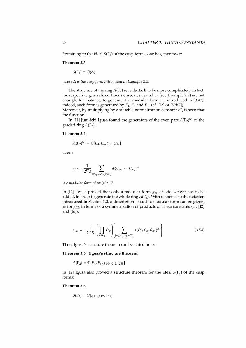
58 CHAPTER 3. THETA CONSTANTS
Pertaining to the ideal S(Γ1) of the cusp forms, one has, moreover:
Theorem 3.3.
S(Γ1) ≡ C(∆)
where ∆ is the cusp form introduced in Example 2.3.
The structure of the ring A(Γ2) reveals itself to be more complicated. In fact,the respective generalized Eisenstein series E4 and E6 (see Example 2.2) are notenough, for instance, to generate the modular form χ10 introduced in (3.42);indeed, such form is generated by E4, E6 and E10 (cf. [I2] or [VdG]).Moreover, by multiplying by a suitable normalization constant c′′, is seen thatthe function:
In [I1] Juni-ichi Igusa found the generators of the even part A(Γ2)(e) of thegraded ring A(Γ2):
Theorem 3.4.
A(Γ2)(e) = C[E4,E6, χ10, χ12]
where:
χ12 =1
2173
∑{mi1 ,...,mi6 }∈C
−
6
±(θmi1· · ·θmi6
)4
is a modular form of weight 12.
In [I2], Igusa proved that only a modular form χ35 of odd weight has to beadded, in order to generate the whole ring A(Γ2). With reference to the notationintroduced in Section 3.2, a description of such a modular form can be given,as for χ12, in terms of a symmetrization of products of Theta constants (cf. [I2]and [I6]):
χ35 = −i
23953
∏m∈C1
θm
∑{mi,m j,mk}∈C−3
±(θmiθm jθmk )20
(3.54)
Then, Igusa’s structure theorem can be stated here:
Theorem 3.5. (Igusa’s structure theorem)
A(Γ2) = C[E4,E6, χ10, χ12, χ35]
In [I2] Igusa also proved a structure theorem for the ideal S(Γ2) of the cuspforms:
Theorem 3.6.
S(Γ2) = C[χ10, χ12, χ35]

3.6. A NEW RESULT: ANOTHER DESCRIPTION FOR χ30 59
The modular form χ35, in particular, admits a factor:
χ30 =18
∑{mi,m j,mk}∈C−3
±(θmiθm jθmk )5 (3.55)
which is is a modular form of weight 30 with a non trivial character (cf. [I2]).Such a modular form is also involved as a generator in another structure theo-rem. By (3.7), the group Γ2/Γ2(2) has only a non trivial irreducible representationof degree 1, corresponding to the sign of the permutation; then, one can denotethe respective character by χP, so that:
χP([γ]) B
1 if ψP([γ]) is an even permutation
−1 if ψP([γ]) is an odd permutation
where ψP is the isomorphism described in (3.6). Then, by setting Γ+2 ⊂ Γ2 the
correspondent subgroup of index two, defined by the condition χP(γ) = 1, onehas the following structure theorem, proved by Igusa in [I2]:
Theorem 3.7.
A(Γ+2 ) = C[E4,E6, χ5, χ12, χ30]
3.6 A new result: another description for χ30
This section is devoted to the presentation of the first new result proposed bythis thesis. A new description will be provided for the modular form χ30, in-troduced in (3.55); to pursue such an aim, the section will need to focus on aparticular construction, described by Bert Van Geemen and Duco Van Stratenin their paper [vGvS].
When g = 2 there are four second order Theta constants, which can be conven-tionally enumerated for the sake of simplicity:
Θ1 B Θ[0 0] Θ2 B Θ[0 1] Θ3 B Θ[1 0] Θ4 B Θ[1 1] (3.56)
Then, (3.49) provides homogeneous relations between the ten first order Thetaconstants and these four ones; more precisely, with reference to the notationintroduced in Example 3.2 for even Theta constants, one has:
θ21 = Θ2
1 + Θ22 + Θ2
3 + Θ24; θ2
2 = Θ21 −Θ2
2 + Θ23 −Θ2
4;
θ23 = Θ2
1 + Θ22 −Θ2
3 −Θ24; θ2
4 = Θ21 −Θ2
2 −Θ23 + Θ2
4;
θ25 = 2Θ1Θ2 + 2Θ3Θ4; θ2
6 = 2Θ1Θ3 + 2Θ2Θ4;
θ27 = 2Θ1Θ4 + 2Θ2Θ3; θ2
8 = 2Θ1Θ2 − 2Θ3Θ4;
θ29 = 2Θ1Θ3 − 2Θ2Θ4; θ2
10 = 2Θ1Θ4 − 2Θ2Θ3;

60 CHAPTER 3. THETA CONSTANTS
A quadratic form Qm in the variables X1,X2,X3,X4 is, therefore, associated toeach even 2-characteristic m ∈ C1:
m 7→ Qm θ2m = Qm(Θ1,Θ2,Θ3,Θ4) (3.57)
Hence, a related quadric Vm in P3 turns out to be associated to each m ∈ C1:
Vm B V(Qm) = {[X1,X2,X3,X4] ∈ P3| Qm(X1,X2,X3,X4) = 0} (3.58)
Proposition 3.20. With reference to the notation introduced in Section 3.2, for each4-plet M ∈ C+
4 , the intersection:⋂m∈Mc
Vm ⊂ P3 (3.59)
is a set of four points in P3.
Proof. Since C+4 is an orbit under the action of Γg, one has only to prove the
statement for a specific element M ∈ C+4 . By focus, in particular, on the 4-plet:
M1 B {m(1),m(2),m(3),m(4)} =
{[0000
],
[0001
],
[0010
],
[0011
]}∈ C+
4 (3.60)
one has:
⋂m∈Mc
Vm = {[1, 0, 0, 0], [0, 1, 0, 0], [0, 0, 1, 0], [0, 0, 0, 1]}
which concludes the proof. �
By Proposition 3.20, for a fixed M ∈ C+4 the four points described in (3.59)
uniquely determine a configuration of four hyperplanes in P3, which are char-acterized by the condition that each of them must pass through all except oneof this points; hence, a collection of four linear forms, describing these fourhyperplanes, is determined by each M ∈ C+
4 :
ψM1 B ψM
1 (X1,X2,X3,X4)
ψM2 B ψM
2 (X1,X2,X3,X4)
ψM3 B ψM
3 (X1,X2,X3,X4)
ψM1 B ψM
1 (X1,X2,X3,X4)
(3.61)
A tetrahedron TM in the projective space P3 turns out thus to be uniquelyassociated to each 4-plet M = (m1,m2,m3,m4) ∈ C+
4 :

3.6. A NEW RESULT: ANOTHER DESCRIPTION FOR χ30 61
M = (m1,m2,m3,m4) 7→ TM (3.62)
in such a way that the vertices are the four points in⋂
m∈Mc Vm and all the pointson the tetrahedron TM are described by the vanishing set:
{ [X1,X2,X3,X4] ∈ P3| FM(X1,X2,X3,X4) = 0 }
where FM B∏4
i=1 ψMi
(3.63)
By a straightforward calculation for each M ∈ C+4 , one is easily supplied with
the linear forms appearing in the related configuration, as described in (3.61):
T1 :
ψ1
1 = X1
ψ12 = X2
ψ13 = X3
ψ14 = X4
T2 :
ψ1
1 = X1 − X3
ψ12 = X1 + X3
ψ13 = X2 − X4
ψ14 = X2 + X4
T3 :
ψ1
1 = X1 − X2
ψ12 = X1 + X2
ψ13 = X3 − X4
ψ14 = X3 + X4
T4 :
ψ4
1 = X1 − X4
ψ42 = X1 + X4
ψ43 = X2 − X3
ψ44 = X2 + X3
T5 :
ψ5
1 = X1 + iX4
ψ52 = X1 − iX4
ψ53 = X2 + iX3
ψ54 = X2 − iX3
T6 :
ψ6
1 = X1 + iX2
ψ62 = X1 − iX2
ψ63 = X3 + iX4
ψ64 = X3 − iX4
T7 :
ψ7
1 = X1 − iX3ψ7
2 = X1 + iX3ψ7
3 = X2 + iX4ψ7
4 = X2 − iX4
T8 :
ψ8
1 = X1 − X2 + X3 − X4
ψ82 = X1 + X2 − X3 − X4
ψ83 = X1 − X2 − X3 + X4
ψ84 = X1 + X2 − X3 + X4
T9 :
ψ9
1 = X1 − X2 − X3 − X4
ψ92 = X1 − X2 + X3 + X4
ψ93 = X1 + X2 + X3 − X4
ψ94 = X1 + X2 − X3 + X4
T10 :
ψ10
1 = X1 + iX2 − X3 − iX4
ψ102 = X1 − iX2 − X3 + iX4
ψ103 = X1 + iX2 + X3 + iX4
ψ104 = X1 − iX2 + X3 − iX4
T11 :
ψ11
1 = X1 + iX2 − X3 + iX4
ψ112 = X1 − iX2 + X3 + iX4ψ11
3 = X1 + iX2 + X3 − iX4
ψ114 = X1 − iX2 − X3 − iX4
T12 :
ψ12
1 = X1 + iX2 + iX3 + X4
ψ122 = X1 + iX2 − iX3 − X4
ψ123 = X1 − iX2 + iX3 − X4
ψ124 = X1 − iX2 − iX3 + X4
T13 :
ψ13
1 = X1 + iX2 − iX3 + X4
ψ132 = X1 + iX2 + iX3 − X4
ψ133 = X1 − iX2 + iX3 + X4
ψ134 = X1 − iX2 − iX3 − X4
T14 :
ψ14
1 = X1 − X2 + iX3 + iX4
ψ142 = X1 − X2 − iX3 − iX4
ψ143 = X1 + X2 + iX3 − iX4
ψ144 = X1 + X2 − iX3 + iX4
T15 :
ψ15
1 = X1 − X2 + iX3 − iX4
ψ152 = X1 − X2 − iX3 + iX4
ψ153 = X1 + X2 − iX3 − iX4
ψ154 = X1 + X2 + iX3 + iX4

62 CHAPTER 3. THETA CONSTANTS
These 15 configurations, describing the tetrahedrons TM, can be used to builda modular forms with respect to the Siegel modular group Γ2. With referenceto the notation introduced in (3.56), a holomorphic function can be associatedto each FM described in (3.63), by:
FM(τ) B FM( Θ1(τ),Θ2(τ),Θ3(τ),Θ4(τ) )
In particular, since T1 is the tetrahedron associated to the 4-plet M1 in (3.60),one has:
F1(τ) B FM1 (τ) = Θ1(τ)Θ2(τ)Θ3(τ)Θ4(τ) = F(2)(τ) (3.64)
which is the modular form of weight 2 with respect to Γ2(2) introduced in (3.48).The product of all the 15 modular forms associated to the configurations is thusa good candidate to study.
To be more precise, one has to remark that Γ2,0(2), as defined in (1.5), is thestabilizer of M1. In fact, by (3.2) one clearly has Γ2,0(2) ⊂ StM1 ; on the otherhand, γ ∈ StM1 implies:
diag(tcγdγ) − cγm′′ ≡ 0 mod 2 ∀m′′ ∈ Z22
which implies cγ ≡ 0 mod 2, hence γ ∈ Γ2,0(2).
Since C+4 is an orbit, one has, therefore:
[Γ2 : Γ2,0(2)] = |C+4 | = 15
Consequently, there exists a bijection between Γ2/Γ2,0(2) and the tetrahedrons,given by the map:
[γ] 7→ TγM1
and one can therefore study the product of all the conjugates of F1 under theaction described in (2.1):
Ψ(τ) B∏
[γ]∈Γ2/Γ2,0(2)
(γ−1|2F1)(τ)
The main theorem of the section can be stated now:
Theorem 3.8. There exists c ∈ C such that:
Ψ = cχ30
where χ30 is the modular form introduced in (3.55).

3.7. RINGS OF MODULAR FORMS WITH LEVELS 63
Proof. By definition of F1 in (3.64) Ψ is a modular form of weight 30 with respectto Γ2(2). Moreover, for
γ0 =
1 0 1 00 1 0 00 0 1 00 0 0 1
∈ Γ2,0(2)
by (3.45), (3.20) and Lemma 3.11, one has:
F1(γ0τ) = −F1(τ)
Then F1 admits a non trivial character under the action of Γ2,0(2). Such acharacter extends to the unique non trivial character χ of Γ2 (cf. [Ib]), henceχ(γγ0γ−1) = χ(γ0) = −1 whenever γ ∈ Γ2. Moreover, with reference to thenotation introduced in (2.2), γ−1
|2F1 ∈ A(γΓ2,0(2)γ−1, χ) for each γ ∈ Γ2, hence:
γ−1γ−10 γ(γ−1
|2F1)(τ) = χ(γγ0γ−1)(γ−1
|2F1)(τ) = χ(γ0)(γ−1|2F1)(τ) = −(γ−1
|2F1)(τ)
Therefore:
(γ−10 |30Ψ)(τ) =
∏[γ]∈Γ2/Γ2,0(2)
(γ−10 γ
−1|2F1)(τ) =
∏[γ]∈Γ2/Γ2,0(2)
(γ−1γγ−10 γ
−1|2F1)(τ) =
=∏
[γ]∈Γ2/Γ2,0(2)
χ(γ0)(γ−1|2F1)(τ) = (−1)15
∏[γ]∈Γ2/Γ2,0(2)
(γ−1|2F1)(τ) =
= (−1)15Ψ(τ)
and consequently Ψ ∈ A(Γ2, χ15 = χ). Hence Ψ must be a multiple of χ30, whichis the only modular form of weight 30 with a non-trivial character. �
Such an expression for χ30 has been also found by Aloys Krieg and DominicGehre in a completely different way, using quaternionic Theta constants (cf.[Kr]).
3.7 Rings of modular forms with levels
This section is devoted to recall important structure theorems for the rings ofmodular forms with respect to some of the congruence subgroups described inthe Section 1.2.
Concerning modular forms with respect to the congruence subgroup Γg(4, 8),Theta constants with characteristics have already been described as a chief ex-ample; indeed their fundamental importance is soon revealed.
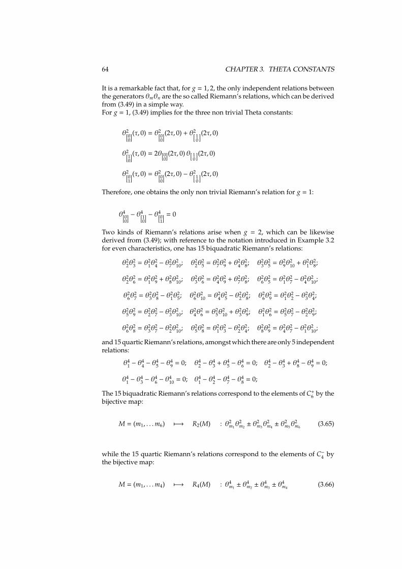
64 CHAPTER 3. THETA CONSTANTS
It is a remarkable fact that, for g = 1, 2, the only independent relations betweenthe generators θmθn are the so called Riemann’s relations, which can be derivedfrom (3.49) in a simple way.For g = 1, (3.49) implies for the three non trivial Theta constants:
θ2[00](τ, 0) = θ2[0
0](2τ, 0) + θ2[
10](2τ, 0)
θ2[10](τ, 0) = 2θ[0
0](2τ, 0)θ[
10](2τ, 0)
θ2[01](τ, 0) = θ2[0
0](2τ, 0) − θ2[
10](2τ, 0)
Therefore, one obtains the only non trivial Riemann’s relation for g = 1:
θ4[00] − θ4[
10] − θ4[0
1] = 0
Two kinds of Riemann’s relations arise when g = 2, which can be likewisederived from (3.49); with reference to the notation introduced in Example 3.2for even characteristics, one has 15 biquadratic Riemann’s relations:
θ22θ
23 = θ2
1θ24 − θ
27θ
210; θ2
2θ25 = θ2
7θ29 + θ2
4θ28; θ2
3θ25 = θ2
9θ210 + θ2
1θ28;
θ22θ
26 = θ2
1θ29 + θ2
8θ210; θ2
3θ26 = θ2
4θ29 + θ2
7θ28; θ2
6θ25 = θ2
1θ27 − θ
24θ
210;
θ26θ
27 = θ2
3θ28 − θ
21θ
25; θ2
6θ210 = θ2
4θ25 − θ
22θ
28; θ2
6θ29 = θ2
1θ22 − θ
23θ
24;
θ25θ
29 = θ2
2θ27 − θ
23θ
210; θ2
4θ26 = θ2
5θ210 + θ2
3θ29; θ2
1θ26 = θ2
5θ27 − θ
22θ
29;
θ26θ
28 = θ2
3θ27 − θ
22θ
210; θ2
5θ28 = θ2
1θ23 − θ
22θ
24; θ2
8θ29 = θ2
4θ27 − θ
21θ
210;
and 15 quartic Riemann’s relations, amongst which there are only 5 independentrelations:
θ41 − θ
44 − θ
45 − θ
49 = 0; θ4
2 − θ43 + θ4
5 − θ46 = 0; θ4
2 − θ43 + θ4
8 − θ49 = 0;
θ41 − θ
43 − θ
46 − θ
410 = 0; θ4
1 − θ42 − θ
47 − θ
48 = 0;
The 15 biquadratic Riemann’s relations correspond to the elements of C+6 by the
bijective map:
M = (m1, . . .m6) 7−→ R2(M) : θ2m1θ2
m2± θ2
m3θ2
m4± θ2
m5θ2
m6(3.65)
while the 15 quartic Riemann’s relations correspond to the elements of C−4 bythe bijective map:
M = (m1, . . .m4) 7−→ R4(M) : θ4m1± θ4
m2± θ4
m3± θ4
m4(3.66)

3.7. RINGS OF MODULAR FORMS WITH LEVELS 65
Denoting by IR the ideal generated by Riemann’s Relations induced on thevariables Xmn = θmθn, one has, as already stated:
C[θmθn] =C[Xmn]
IR(g = 1, 2) (3.67)
For g ≥ 3 Riemann’s relations still provide independent relations between thegenerators θmθn; it is still not known, however, whether they are the onlyindependent relations between generators for the ring C[θmθn] or not.Concerning the ring in (3.67), one has:
Theorem 3.9. The ring C[θmθn] is normal when g = 1, 2.
Proof. The proof can be found in [I3] for the case g = 1 and in [I2] for the caseg = 2. �
The ring C[θmθn] reveals itself to be strictly connected with the modular formswith respect to the congruence subgroup Γg(4, 8) as a classical result proved byIgusa in [I3] states:
Theorem 3.10. (Igusa’s structure theorem) A(Γg(4, 8)) is the normalization of thering C[θmθn].
A straight consequence of Theorem 3.9 is the following:
Corollary 3.10. A(Γg(4, 8)) = C[θmθn] when g = 1, 2.
The section ends by recalling a structure theorem for cusp forms with respectto the subgroup Γ2(2, 4, 8) defined in (1.8), which will be used in the next chapterto prove new results; this structure theorem was proved by van Geemen andvan Straten in [vGvS], also using the construction already described in Section3.6.
Theorem 3.11. (van Geemen, van Straten) A set of generators for the idealS(Γ2(2, 4, 8)) of the cusp forms with respect to Γ2(2, 4, 8) is given by:
1. D(M) ∀M ∈ C−4
2. θm1θm2θm3θm4θm5 ∀ {m1 . . . ,m5} < C+5 ∪ C−5
3. θm1θm2θm3ψMi , ψ
Mj , ψ
Mk ∀ {m1,m2,m3} ∈ C+
3 ∀ i, j, k
where, for each {m1,m2,m3} ∈ C+3 , M ∈ C+
4 the only element such that {m1,m2,m3} ⊂
M and ψMi , ψ
Mj , ψ
Mk are three of the linear forms associated to TM as in (3.61).

66 CHAPTER 3. THETA CONSTANTS

Chapter 4
The group Γ and the structureof A(Γ) and S(Γ)
The aim of this chapter is to present the new results found, concerning a re-markable map made by the gradients of odd Theta functions in genus 2. Thefirst section will be devoted to outline the general description of this map, thuspointing out the exceptional features pertaining to the case g = 2, on which theother sections will be focused.Since every statement concerning the new results will pertain to the case g = 2,the obvious indication of the grade g = 2 will be conventionally omitted.For the sake of simplicity, the group Γ(2, 4)/{±Γ(4, 8)}, which will turn out to beinvolved in the discussion, will be denoted by the symbol G, while the symbolG will stand for the group of characters of G.
4.1 The Theta Gradients Map
By the transformation formula (3.34) one is allowed to define a map on thequotient space A4,8
g B Sg/Γg(4, 8):
PgrTh : A4,8g −→
2g−1(2g−1)times︷ ︸︸ ︷
Cg× · · · × Cg/T0(Gl(g,C))
τ −→{gradzθn|z=0
}n odd
where T0 is the representation defined in (3.35).
As a consequence of Lefschetz’s theorem (cf. [GH]) the range of this map liesin the Grassmannian GrC(g, 2g−1(2g
− 1)), as proved by Riccardo Salvati Manniin [SM1]. The Jacobian determinants are the Plucker coordinates of this map.In their work [GSM], Samuel Grushevsky and Riccardo Salvati Manni provedthat this map is generically injective on A4,8
g when g ≥ 3 and injective on thetangent spaces when g ≥ 2.
67

68 CHAPTER 4. THE GROUP Γ AND THE STRUCTURE OF A(Γ) AND S(Γ)
The map was also conjectured to be injective whenever g ≥ 3, albeit it has notbeen proved yet.
The case g = 2 reveals itself, indeed, to be a case of special interest. The sixodd 2-characteristics originate fifteen Jacobian determinants, namely the onesenumerated in Example 3.2, which satisfy by (3.36) the following transforma-tion law:
D(N)(γτ) = κ(γ)2χN(σ)det(cγτ + dγ)2D(N)(τ)
∀ τ ∈ S2 ∀γ ∈ Γ2(2, 4) ∀N = {n1,n2} ∈ C2
(4.1)
where χN = χn1χn2 .The respective Theta gradients map in these fifteen Plucker coordinates is:
PgrTh : A4,8−→ P14
τ −→ { [ D(N)(τ) ] }N∈C2
which can not be injective by (1.7), but is seen to be finite.
However, there exists a suitable intermediate congruence subgroup Γ(4, 8) ⊂Γ ⊂ Γ(2, 4) such that the Theta gradients map factors on the correspondent levelmoduli space AΓ B Sg/Γ as:
PgrTh∗ : AΓ2 → P14 AΓ
2 B S2/Γ
and the new map PgrTh∗ turns out to be injective.
In the following section such a remarkable group will be described.
4.2 The congruence subgroup Γ
As already explained, the chief interest of this section is to locate betweenΓ(4, 8) and Γ(2, 4) the right congruence subgroup Γ, whose correspondent levelmoduli space AΓ B Sg/Γ is such that the Theta gradients map PgrTh is stillwell defined on it and injective. The following description is provided for sucha group:
Proposition 4.1.
Γ =
15⋂i=1
KerχNi = {γ ∈ Γ(2, 4) | κ(γ)2χNi (γ) = 1 ∀i = 1, . . . , 15} (4.2)
where χNi are the fifteen characters involved in the transformation law (4.1) forthe fifteen Jacobian determinants.

4.2. THE CONGRUENCE SUBGROUP Γ 69
Proof. As far as one knows by (4.1), an a priori description for the subgroup Γis:
Γ B Γ(1)∪ Γ(−1) (4.3)
where:
Γ(1) B {γ ∈ Γ(2, 4) | κ(γ)2χNi (γ) = 1 ∀i = 1, . . . , 15}
Γ(−1) B {γ ∈ Γ(2, 4) | κ(γ)2χNi (γ) = −1 ∀i = 1, . . . , 15}
Γ, as defined in (4.3) is plainly checked to be a subgroup of the Siegel modulargroup Γ2, for Corollary 3.7 and Lemma 3.15 imply for each i = 1, . . . , 15:
κ2(γγ′)χNi (γγ′) = κ2(γ)χNi (γ)κ2(γ′)χNi (γ
′) = 1
κ2(γ−1)χNi (γ−1) = [κ2(γ)χNi (γ) ]−1 = κ2(γ)χNi (γ)
∀γ, γ′ ∈ Γ
Moreover, by (3.22) and Lemma 3.16, one has Γ(4, 8) ⊂ Γ; hence the subgroupΓ, as defined in (4.3), is indeed a congruence subgroup such that Γ(4, 8) ⊂ Γ ⊂Γ(2, 4).
The next step is to refine the definition of Γ, by detecting which elements ofΓ(2, 4) belong to this subgroup.
Clearly⋂15
i=1 KerχNi ⊂ Γ. Therefore, the reverse inclusion has only to be shown,to prove the first part of the statement.Let thus γ ∈ Γ. Due to the definition in (4.3), either χNi (γ) = 1 for eachi = 1, . . . , 15 or χNi (γ) = −1 for each i = 1, . . . , 15. However, if χNi (γ) = −1, foreach i, an absurd statement turns up:
−1 = χ(n,ni)(γ)χ(n,n j)(γ)χ(n,nk)(γ) = χ(ni,n j)(γ)χ(n,nk) (γ) = 1
Hence, the only possible case is γ ∈⋂15
i=1 KerχNi .Consequently, one has:
Γ =
15⋂i=1
KerχNi (4.4)
and this part of the statement is proved.In order to obtain the second identity in the statement, one needs to prove thatk2(γ) = 1 whenever γ ∈ Γ. By the criterion described in Proposition 3.19, theproducts:
D B D(n1,n2)D(n3,n4)D(n5,n6)
with n1, . . .n6 all distinct, are plainly checked to be modular forms with respectto Γ(2, 4). Moreover, by (4.1), the following transformation law is satisfied foreach γ ∈ Γ(2, 4):

70 CHAPTER 4. THE GROUP Γ AND THE STRUCTURE OF A(Γ) AND S(Γ)
D(γτ) = k2(γ)χn1 · · ·χn6 det(cγτ + dγ)6D(τ)
Hence, by (3.14), one has for each γ ∈ Γ(2, 4):
k2(γ) =
6∏i=1
χni (γ) = χ(n1,n2)(γ)χ(n3,n4)(γ)χ(n5,n6)(γ)
Therefore, whenever γ ∈ Γ, k2(γ) = 1 by the characterization in (4.4). Thisshows Γ(−1) in (4.3) is indeed an empty set, and Γ = Γ(1). This concludes theproof.
�
Thanks to the description of the congruence subgroup Γ provided in Proposi-tion 4.1, an important property can be immediately stated:
Proposition 4.2. Γ is normal in Γ2.
Proof. One has to prove that:
χNi (γ−1ηγ) = 1 ∀γ ∈ Γ2 , ∀η ∈ Γ , ∀i = 1, . . . , 15
By setting Ni = (n1 i,n2 i) for each i = 1, . . . , 15, one has:
χNi (γ−1ηγ) = χn1 i (γ
−1ηγ)χn2 i (γ−1ηγ) = γ−1(χn1 i , χn2 i )(η) = χγn1 i (η)χγn2 i (η)
Since the action in (3.2) preserves the parity, for each i = 1, . . . , 15 there exists aj, depending on i and γ, such that (γn1 i, γn2 i) = N j. Therefore:
χN j (γ−1ηγ) = χγn1 i (η)χγn2 i (η) = χN j (η) = 1
where the last equality on the right holds since η ∈ Γ. �
As a straight consequence, one has the following:
Corollary 4.1. S2 does not admit any fixed point for the action of Γ. In particular, thespace S2/Γ is smooth.
Proof. Since Γ ⊂ Γ(2, 4), the thesis follows from Corollary 1.5 and Proposition4.4. �
A concrete description for the congruence subgroup Γ in terms of generatorscan be also a useful tool to work with. Corollary 3.9 suggests how to find sucha description.Since the functions χNi are characters of the group G = Γ(2, 4)/{±Γ(4, 8)}, onecan find the elements in Γ(2, 4), which belongs to
⋂15i=1 KerχNi , by checking just
the representative elements for the cosets in {±Γ(4, 8)} in Γ(2, 4).For such a purpose, Proposition 1.3 and Corollary 1.2 can be applied, to obtain:

4.2. THE CONGRUENCE SUBGROUP Γ 71
Proposition 4.3. The group G is a 9-dimensional vector space onZ2. A basis is givenby:
A11 =
−1 0 0 00 1 0 00 0 −1 00 0 0 1
A12 =
1 2 0 00 1 0 00 0 1 00 0 −2 1
A21 =
1 0 0 02 1 0 00 0 1 −20 0 0 1
B2
11 =
1 0 4 00 1 0 00 0 1 00 0 0 1
B222 =
1 0 0 00 1 0 40 0 1 00 0 0 1
B12 =
1 0 0 20 1 2 00 0 1 00 0 0 1
C2
11 =
1 0 0 00 1 0 04 0 1 00 0 0 1
C222 =
1 0 0 00 1 0 00 0 1 00 4 0 1
C12 =
1 0 0 00 1 0 00 2 1 02 0 0 1
Then, by setting χi, j B χ(n(i),n( j)) for each i, j, with reference to the notationintroduced in Example 3.2 for odd characteristics, a simple table can be redactedby a straightforward computation, using (3.23) and the values in Lemma 3.13:
A11 A12 A21 B12 B211 B2
22 C12 C211 C2
22χ12 -1 1 1 1 -1 -1 1 -1 -1χ13 1 1 -1 1 1 1 -1 -1 1χ14 -1 -1 1 1 -1 -1 -1 -1 1χ15 1 -1 1 -1 -1 1 1 1 1χ16 -1 1 -1 -1 -1 1 1 -1 -1χ23 -1 1 -1 1 -1 -1 -1 1 -1χ24 1 -1 1 1 1 1 -1 1 -1χ25 -1 -1 1 -1 1 -1 1 -1 -1χ26 1 1 -1 -1 1 -1 1 1 1χ34 -1 -1 -1 1 -1 -1 1 1 1χ35 1 -1 -1 -1 -1 1 -1 -1 1χ36 -1 1 1 -1 -1 1 -1 1 -1χ45 -1 1 1 -1 1 -1 -1 -1 1χ46 1 -1 -1 -1 1 -1 -1 1 -1χ56 -1 -1 -1 1 1 1 1 -1 -1
The independent elements satisfying the desired properties can be easily de-tected by this table, to state the following:

72 CHAPTER 4. THE GROUP Γ AND THE STRUCTURE OF A(Γ) AND S(Γ)
Proposition 4.4. The group Γ is generated by Γ(4, 8) and the elements:
A12B211C2
22 =
1 2 4 00 1 0 00 0 1 00 4 −2 1
t(A12B2
11C222) = A21B2
22C211 =
1 0 0 02 1 0 44 0 1 −20 0 0 1
B12B2
11B222 =
1 0 4 20 1 2 40 0 1 00 0 0 1
t(B12B2
11B222) = C12C2
11C222 =
1 0 0 00 1 0 04 2 1 02 4 0 1
4.3 Structure of A(Γ): generators
Since the Plucker coordinates D(N) are known to be cusp forms, the Theta gra-dients map does not extend to the boundary of Satake’s compactification 1 ofthe level moduli space A4,8. The graded ring A(Γ) of the modular forms withrespect to the congruence subgroup Γ, as well as the ideal S(Γ) ⊂ A(Γ) of thecusp forms, are needed to describe the Satake’s compactification ProjA(Γ) andthe desingularization ProjS(Γ) of the map on it. The respective even parts A(Γ)e
and S(Γ)e are, indeed, the only relevant part in describing the Proj scheme 2.This work is therefore interested in describing the structure of A(Γ)e and S(Γ)e;as a first step, this section will aim, in particular, to find generators for A(Γ)e Astructure theorem have to be proved first, in order to describe A(Γ)e:
Proposition 4.5. Let χ5 B∏10
i=1 θmi be the modular form introduced in (3.40). Then:
A(Γ(4, 8)) =
⊕d even
C[θ2mθ
2n]θm1 · · ·θm2d
⊕ ⊕
h=0,2,4
C[θ2mθ
2n]
χ5
θm1 · · ·θm2h
where:
A(Γ(4, 8))e =⊕d even
C[θ2mθ
2n]θm1 · · ·θm2d
is the even part of the graded ring, and
1See Appendix B2A detailed exposition of these topics can be found, for instance, in the classic book [Ht].

4.3. STRUCTURE OF A(Γ): GENERATORS 73
A(Γ(4, 8))o =⊕
h=0,2,4
C[θ2mθ
2n]
χ5
θm1 · · ·θm2h
is the odd part.
Proof. By Igusa’s Theorem, A(Γ(4, 8) = C[θmθn] (Corollary 3.10); the result of thedecomposition of the ring under the action of Γ(2, 4), according to the generalprocedure described in (2.2), is then:
A(Γ(4, 8)) =⊕χ∈G
C[θmθn, χ]
Since monomials in Theta constants transforms into monomials under the ac-tion of Γ(2, 4) (by (3.36)), one needs to focus only on monomials inθmθn, in orderto study the transformation law for elements of C[θmθn] under this action.
In particular, if Pd = θm1 · · ·θm2d ∈ C[θmθn]d is a monomial of degree d in thevariables θmθn, (3.36) implies the following transformation law:
Pd(γτ) = κ2d(γ)χm1 · · ·χm2d det (cγτ + dγ)dPd(τ) ∀γ ∈ Γ(2, 4)
If d = 2l, Pd ∈ C[θmθn, χm1 · · ·χm2d ], because κ4(γ) = 1 for each γ ∈ Γ(2, 4) by(3.22). Moreover, Corollary 3.9 and Lemma 3.14 imply that for each couple ofcharacteristics m,n, the product χ2
mχ2n is a trivial character of G ; the following
decomposition arises, therefore, for the even part A(Γ(4, 8))e of the ring:
A(Γ(4, 8))e =⊕d even
C[θ2mθ
2n]θm1 · · ·θm2d (4.5)
On the other hand, if d = 2l + 1, Pd ∈ C[θmθn, κ2χm1 · · ·χm2d ]. Moreover, sinceχm1 · · ·χm10 = 1 on Γ(2, 4), (3.41) implies the following transformation law forχ5:
χ5(γτ) = κ2(γ) det (cγτ + dγ)5χ5(τ) ∀γ ∈ Γ(2, 4)
Therefore, for each sequence M = {m1, . . .m2h} of even characteristics, one has:
χ5
θm1 · · ·θm2h
∈ C[θmθn, χMc ]
Since κ2 is a character of G, as stated in Corollary 3.7, it is indeed a product ofthe functions χm by Proposition 3.11; the following decomposition arises, then,for the odd part A(Γ(4, 8))o of the ring:

74 CHAPTER 4. THE GROUP Γ AND THE STRUCTURE OF A(Γ) AND S(Γ)
A(Γ(4, 8))o =⊕
h=0,2,4
C[θ2mθ
2n]
χ5
θm1 · · ·θm2h
(4.6)
This concludes the proof.�
Thanks to Proposition 4.5 a structure theorem can be finally stated for A(Γ)e.
Theorem 4.1. A(Γ)e = C[θ2mθ
2n,D(N)].
Proof. By Proposition 4.1, Γ/{±Γ(4, 8)} ⊂ G is the dual subgroup correspondingto the subgroup < χNi >⊂ G generated by the fifteen characters χNi related tothe Jacobian determinants D(Ni). One has, therefore:
A(Γ) =⊕
χ∈<χNi>
A(Γ(4, 8), χ)
Hence, the thesis follows from (4.5). �
4.4 Structure of A(Γ): relations
The foregoing section has been devoted to the detection of the generators ofA(Γ)e, which have turned out to beθ2
mθ2n and D(N). Some relations exist amongst
these generators, most of which are induced by Riemann’s relations. This sec-tion aims to provide them, by a combinatorial description. For this purpose athreefold investigation will be needed, in order to find the relations involvingonly the θ2
mθ2n, the relations involving only the D(N), and finally the ones be-
tween the θ2mθ
2n and the D(N).
4.4.1 Relations among θ2mθ
2n
The relations amongθ2mθ
2n are completely described by Riemann’s relations (see
Section 3.7). Therefore, with reference to the notation introduced in (3.65) and(3.66), there are 15 independent biquadratic relations:
R2(M) = 0 ∀M ∈ C+6 (4.7a)
and 5 independent quartic relations:
R4(Mi) = 0 i = 1, . . . 5 (4.7b)

4.4. STRUCTURE OF A(Γ): RELATIONS 75
4.4.2 Relations among D(N)
The 15 relations of the kind:
D(M)2 = θ2m1θ2
m2θ2
m3θ2
m4∀M = {m1,m2,m3,m4} ∈ C−4
induced by Jacobi’s formula and described in Example 3.2, have to be usedtogether with the ones in (4.7a) and (4.7b), to find all the desired relationsamongst the fifteen Jacobian determinants {D(M)}M∈C−4 . These have been doneby Professor Eberhard Freitag by means of a computer program written by him;here a combinatoric explanation follows for all the relations found.
1. For each even characteristic m, one can enumerate the six 4-plets {Mmi }i=1,...6
in C−4 containing m, in such a way that:
Mm1 ∩Mm
2 ∩Mm3 = {m} = Mm
4 ∩Mm5 ∩Mm
6
Then, one has:
D(Mm1 )D(Mm
2 )D(Mm3 ) = χ5θ
2m = D(Mm
4 )D(Mm5 )D(Mm
6 ) (4.8a)
which are obviously 10 relations, namely one for each choice of m.
2. For each M = {m1, . . .m6} ∈ C+6 there are eight 4-plets of C−4 , containing
exactly a triplet {mi,m j,mk} ⊂M; these 4-plets can be enumerated in sucha way that:
D(M1)D(M2)D(M3)D(M4) = χ5∏6
i=1 θ2mi
=
= D(M5)D(M6)D(M7)D(M8)(4.8b)
These are 15 relations, namely one for each choice of M ∈ C+6 .
3. Let M = {m1, . . .m6} ∈ C+6 and let
R2(M) = θ2m1θ2
m2± θ2
m3θ2
m4± θ2
m5θ2
m6= 0
be the associated biquadratic Riemann’s relation as in (3.65).For each couple of even characteristics {mi,m j}, one can denote by Mi, j
1
and Mi, j2 the only two 4-plets of C−4 containing {mi,m j}; then, one has:
D(M1,21 )D(M1,2
2 ) ±D(M3,41 )D(M3,4
2 ) ±D(M5,61 )D(M5,6
2 ) =
= ±D(M′)R2(M) = 0(4.8c)

76 CHAPTER 4. THE GROUP Γ AND THE STRUCTURE OF A(Γ) AND S(Γ)
These are 15 relations, since they correspond to the elements of C+6 .
Otherwise, by choosing for each couple of even characteristics mi,m j onlyone of the two 4-plets Mi, j
1 e Mi, j2 , one has the following general identity:
D2(M1,2α ) ±D2(M3,4
β ) ±D2(M5,6ε ) =
= θ2α1θ2α2θ2
m1θ2
m2± θ2
β1θ2β2θ2
m3θ2
m4± θ2
ε1θ2ε2θ2
m5θ2
m6
where α1, α2, β1, β2, ε1, ε2 are characteristics in Mc∈ C−4 .
In particular, each triplet of determinants can be chosen in such a waythat only three of the four characteristics appearing in the 4-plet Mc areinvolved in the respective identity; for combinatorial reasons, there isa unique way to build a relation among D(M)’s by multiplying eachdeterminant of such a triplet by two other distinct determinants:
Dh Dk D2(M1,2α ) ±Dl Dr D2(M3,4
β ) ±Ds Dt D2(M5,6ε ) = 0 (4.8d)
One can observe that, for each choice of M ∈ C+6 , there exist four distinct
triplets of determinants D(M1,2α ),D2(M3,4
β ),D2(M5,6ε ) satisfying the desired
condition; more precisely, each triplet corresponds to a choice for thecharacteristic in Mc which does not appear in the identity, and obviouslythere are four possible choices for such a characteristic. Therefore, therelations (4.8d) are in number of 15 · 4 = 60.
4. Let M = {m1, . . .m4} ∈ C−4 an let
R4(M) = θ4m1± θ4
m2± θ4
m3± θ4
m4= 0
be the associated quartic Riemann’s relation as in (3.66). For each mi ∈Mthere exist only 2 elements Mi
1,Mi2 ∈ C−4 containing mi and such that:
Mi1 MMi
2 = Mc = {m5, . . .m10}
One has, therefore:
4∑i=1
±D(Mi1)2 D(Mi
2)2 = θm5 · · ·θm10 R4(M) = 0 (4.8e)
It must be remarked that all the 15 quartic Riemann relations induce in-dependent relations on the D(M), even though they are not independentthemselves; the relations in (4.8e) are, therefore, in number of 15.

4.4. STRUCTURE OF A(Γ): RELATIONS 77
5. Let M = {m1,m2,m3} ∈ C−3 be fixed.There exist only two distinct 6-plets in C+
6 , containing M. Then let M ={m1,m2,m3,m′1,m
′
2,m′
3} be such a 6-plet; the corresponding biquadraticRiemann’s relation is easily seen to be such that:
R2(M) = θ2m1θ2
m′1± θ2
m2θ2
m′2± θ2
m3θ2
m′3= 0
with {m′1,m′
2,m′
3} ∈ C−3 .Moreover, for each couple of characteristics {mi,m j} ⊂ M, there exists aunique Mi, j ∈ C+
6 , containing {mi,m j} and satisfying:
R2(Mi, j) = ±θ2miθ2
m j+ Pi j = 0
For combinatorial reasons, all the terms θ2m′i
P j,k share the common addend
θ2m′1θ2
m′2θ2
m′3; therefore, one has:
0 = θ2m1θ2
m2θ2
m3R2(M) = ±θ2
m1θ2
m′1P2,3 ± θ
2m2θ2
m′2P1,3 ± θ
2m3θ2
m′3P1,2 =
= ±θ2m4θ2
m′1θ2
m′2θ2
m′3± θ2
m1θ2
m′1θ2
mαθ2
mβ± θ2
m2θ2
m′2θ2
mαθ2
mε± θ2
m3θ2
m′3θ2
mβθ2
mε
where m4 is the unique even characteristic which completes M = {m1,m2,m3}
to a 4-plet in C−4 (to which a quartic Riemann’s relations correspond, as in(3.66)), and {mα,mβ,mε} = {m1,m2,m3,m4,m′1,m
′
2,m′
3}c.
Then it is easily checked that:
0 =
∏m<{m1,m2,m3,m4}
θm
θ2m1θ2
m2θ2
m3R2(M) =
4∑i=1
±D(Mi1) D(Mi
2)3 (4.8f)
where Mi1 and Mi
2 are, for each i = 1, . . . 4, the 4-plets in C−4 containingmi and such that Mi
1 M Mi2 = {m1,m2,m3,m4}
c, already appeared in therelations (4.8e).By selecting the other 6-plet M = {m1,m2,m3,mα,mβ,mε} containing M ={m1,m2,m3}, one obtains the same relations with interchanged exponents:
0 =
4∑i=1
±D(Mi1)3 D(Mi
2) (4.8g)
One has to observe that triplets M = {m1,m2,m3} belonging to the same 4-plet in C−4 produce exactly the same relation (essentially because the samerelated quartic Riemann relation comes substituted in the foregoing nullexpression). Therefore, these relations are parameterized by the elementsin C−4 ; consequently, there are 15 relations of the type (4.8f) and 15 of thetype (4.8g).

78 CHAPTER 4. THE GROUP Γ AND THE STRUCTURE OF A(Γ) AND S(Γ)
6. For each even characteristic m ∈ C1, there are exactly six determinants{Dm
i }i=1,...6 such that:
Dmi = D(M) = ±θm1θm2θm3θm4 with m ∈M = {m1,m2,m3,m4} ∈ C−4
Then, one has:
6∑i=1
(Dmi )4 = θ4
m[θ4n1
(θ4α1θ4α3± θ4
α2θ4α4
)±
± θ4n2
(θ4α1θ4α5± θ4
α2θ4α6
) ± θ4n3
(θ4α3θ4α5± θ4
α4θ4α6
)]
where {α1, α2, α3, α4}, {α1, α2, α5, α6} ∈ C−4 .Then, for each i, j, k = 1, . . . 6 such that {αi, α j, αk} ∈ C−3 , one can denote bythe symbol Mk
i j the only 4-plet in C−4 containing αi, α j, and not αk, and by
the symbol P(Mki j) the polynomial:
P(Mki j) B R4(Mk
i j) − θ4α j
where R4(Mki j) is the quartic Riemann relation associated to Mk
i j as in (3.66).Then, in particular:
6∑i=1
±(Dmi )4 = θ4
m{θ4n1
[θ4α1
P(M123) ± θ4
α2P(M2
14)]±
± θ4n2
[θ4α1
P(M125) ± θ4
α2P(M2
16)] ± θ4n3
[θ4α3
P(M345) ± θ4
α4P(M4
36)]}
where:
M1
23 ∩M214 = {n2,n3}
M125 ∩M2
16 = {n1,n3}
M345 ∩M4
36 = {n1,n2}
Therefore, for a suitable choice of the relative signs, one has:
6∑i=1
± (Dmi )4 = θ4
m[θ4n1
(θ4α1± θ4
α2)(±θ4
n2± θ4
n3)±
θ4n2
(θ4α1± θ4
α2)(±θ4
n1± θ4
n3) ± θ4
n3(θ4α1± θ4
α2)(±θ4
n1± θ4
n2)] =
= θ4m(θ4
α1± θ4
α2)[θ4
n1(±θ4
n2± θ4
n3) ± θ4
n2(±θ4
n1± θ4
n3) ± θ4
n3(±θ4
n1± θ4
n2)]

4.4. STRUCTURE OF A(Γ): RELATIONS 79
which is made null by a suitable choice for the remaining signs. To sumup, therefore, for each m ∈ C1 one has the relation:
6∑i=1
±(Dmi )4 = 0 (4.8h)
with a suitable choice of the signs, uniquely determined as explained.However, it is easily verified that only 6 of this ten relations are indepen-dent.
Now, the following definitive Proposition can be stated concerning therelations among the D(N):
Proposition 4.6. All the relations amongst the D(N) are generated by:
1. The 10 relations in (4.8a);
2. The 15 relations in (4.8b);
3. The 15 relations in (4.8c);
4. The 60 relations in (4.8d);
5. The 15 relations in (4.8e);
6. The 15 relations in (4.8f);
7. The 15 relations in (4.8g);
8. The 6 relations in (4.8h);
Proof. The statement has been proved computationally by elimination theory,thanks to a computer program created by Professor Eberhard Freitag. �
4.4.3 Relations among D(N) and θ2mθ
2n
There are of course the 15 relations induced by the Jacobi’s formula:
D(M)2 = θ2m1θ2
m2θ2
m3θ2
m4∀M = {m1,m2,m3,m4} ∈ C−4 (4.9a)
as described in Example 3.2. Any other relation is clearly generated by the onesin (4.9a) and by all the relations of the kind:
h∏i=1
D(Ni) = P(θ2mθ
2n)
where P(θ2mθ
2n) is a polynomial in θ2
mθ2n and the determinants D(Ni) are all
distinct.

80 CHAPTER 4. THE GROUP Γ AND THE STRUCTURE OF A(Γ) AND S(Γ)
Since for each couple of characteristics m,n θ2mθ
2n is a modular form with respect
to Γ(2, 4) by (3.36) and (3.23), such a relation is satisfied if and only if∏
i D(Ni)itself is a modular form with respect to Γ(2, 4).By Proposition 3.14 such a condition is equivalent to MtM ≡ 0 mod2 for the 4×4hmatrix M = (M1 . . .Mh) of even characteristics, associated to
∏i D(Mi), and also,
by Proposition 3.19, to NtN ≡ 0 mod2 on the 4 × 2h matrix N = (N1 . . .Nh) ofodd characteristics, associated to
∏i D(Ni). A necessary condition is therefore
given by:
diag(MtM) ≡ 0 mod 2
or, likewise, concerning odd characteristics, by:
diag(NtN) ≡ 0 mod 2
As a first step, the discussion will be therefore focused on products∏
i D(Ni)of distinct Jacobian determinants, satisfying this condition. For such a purposethe following technical definition will be useful throughout this section:
Definition 4.1. Let 1 ≤ h ≤ 15, and let D(N1) · · ·D(Nh) = D(M1) · · ·D(Mh) be aproduct of distinct Jacobian determinants. If the sum of all the even characteristics mappearing in the 4plets Mi ∈ C−4 (or, equivalently, the sum of all the odd characteristicsn appearing in the couples N ∈ C2), each counted with its multiplicity, is congruent to0 mod 2, such a product will be called a remarkable factor of degree h. A remarkablefactor which is product of remarkable factors will be named reducible, otherwise itwill be called non-reducible.
As already seen, if the product D(N1) · · ·D(Nh) of distinct determinants is amodular form with respect to Γ(2, 4), it is a remarkable factor, while the con-verse statement is not necessarily true.
Remarkable factors can be easily characterized.
Proposition 4.7. P is a remarkable factor if and only if P is a monomial in the variablesθ2
m and χ5. More precisely:
P = χ5h∏
m
θm2 h = 0, 1
Proof. If P is a monomial in the variables θ2m and χ5, then P is clearly a remark-
able factor; therefore, only the converse statement has to be proved .For such a purpose, one can use the function, defined in (3.52):
F : C −→ C[θm]
{m1,m2, . . . ,mh} −→ θm1θm2 · · ·θmh
F(∅) B 1
Then, in particular:
F({m}) = θm; F(C1) = χ5; F(M) = D(M) ∀M ∈ C−4 ;

4.4. STRUCTURE OF A(Γ): RELATIONS 81
and moreover one has:
F(Mi) F(M j) = F(M1 MM j)∏
m∈Mi∩M j
θm2
If P = F(M1) · · · F(Mh) is a remarkable factor, by using such identity and Propo-sitions 3.4, 3.5 and 3.6, it necessarily follows that:
P = χ5h∏
m
θm2
with h = 0, 1. �
In order to classify remarkable factors in terms of the Jacobian determinantsappearing in the product, the law which associates to each couple of oddcharacteristics N ∈ C2 their sum S(N) ∈ Z4
2 will be a useful tool:
N = {n1,n2} −→ S(N) B n1 + n2
In fact, a product P =∏
i D(Ni) of distinct Jacobian determinants is clearly aremarkable factor if and only if
∑i S(Ni) = 0.
Lemma 4.1. Remarkable factors of degree greater than 5 are reducible.
Proof. Let P =∏h
i=1 D(Ni) be a remarkable factor with h > 5. The set {S(Ni)}i=1,...h ⊂
Z42 necessarily contains at least two elements linearly dependent from the oth-
ers. Since S(N) , 0 for each N ∈ C2, the thesis follows. �
By Lemma 4.1, remarkable factors of degree at most 5 are the only ones to check,in order to find the non-reducible ones.
Proposition 4.8. Non-reducible factors are:
1. D(ni,n j)D(n j,nk)D(nk,ni);
2. D(ni,n j)D(nk,nl)D(ns,nt);
3. D(ni,n j)D(n j,nk)D(nk,nl)D(nl,ni);
4. D(ni,n j)D(ni,nk)D(ni,nl)D(ns,nt);
5. D(ni,n j)D(n j,nk)D(nk,nl)D(nl,nr)D(nr,ni);
6. D(n,n j)D(n,nk)D(n,nl)D(m,nr)D(m,ns);
Proof. They can be plainly detected by the following table, which can beredacted with reference to the notation introduced in the Example 3.2 for oddcharacteristics:
�

82 CHAPTER 4. THE GROUP Γ AND THE STRUCTURE OF A(Γ) AND S(Γ)
D(N) tS(N)D(n(1),n(2)) (1111)D(n(1),n(3)) (0010)D(n(2),n(3)) (1101)D(n(1),n(4)) (1110)D(n(2),n(4)) (0001)D(n(1),n(5)) (1000)D(n(2),n(5)) (0111)D(n(1),n(6)) (1011)D(n(2),n(6)) (0100)D(n(3),n(4)) (1100)D(n(3),n(5)) (1010)D(n(3),n(6)) (1001)D(n(4),n(5)) (0110)D(n(4),n(6)) (0101)D(n(5),n(6)) (0011)
By using (3.19), one can observe that only the factors of the type 2., 3. and 6. aremodular forms with respect to Γ(2, 4). As a consequence of Proposition 4.7, χ5appears in such factors with even multiplicity, while it appears in the factors oftype 1., 4. and 5. χ5 with odd multiplicity.
The products∏
i D(Ni) of distinct determinants which are functions of θ2mθ
2n,
are thus necessarily products of the factors listed in Proposition 4.8.
Proposition 4.9. The relations involving products of 3 determinants are:
D(ni,n j)D(nk,nl)D(ns,nt) =
6∏i=1
θmi2 (4.9b)
Proof. As already stated, the factors of type 2. are the only ones involved.In order to prove that the six Theta constants appearing in the expression (4.9b)are all distinct, let P be a product of determinants of the type in (4.9b), and letM1,M2,M3 ∈ C−4 be the 4-plets satisfying:
P = D(M1)D(M2)D(M3)
Since P is a remarkable factor, if Mi M M j ∈ C+6 for any couple of this 4-plets, it
would follow that (M1 MM2)c = M3; then one would have P = θm12θm2
2θm32χ5,
which is an absurd statement, because P is also a modular form with respect toΓ2(2, 4). Then, by Proposition 3.4, Mi MM j ∈ C−4 for each distinct couple Mi,M j,and the only possibility is M1 MM2 = M3 ∈ C−4 , namely:
M1 = {m1,m2,m3,m4} M2 = {m1,m2,m5,m6} M3 = {m3,m4,m5,m6}
Therefore, the thesis follows. �
Proposition 4.10. The relations involving products of 4 determinants are:

4.4. STRUCTURE OF A(Γ): RELATIONS 83
D(ni,n j)D(n j,nk)D(nk,nl)D(nl,ni) =
8∏i=1
θmi2 (4.9c)
Proof. Remarkable factors of type 3. are the only ones involved.To prove the eight Theta constants appearing in the expression (4.9c) are alldistinct, let P be a product of determinants of the type in (4.9c), and letM1,M2,M3,M4 ∈ C−4 the 4-plets satisfying:
P = D(M1)D(M2)D(M3)D(M4)
If M1 M M2 ∈ C−4 , then M3 M M4 = M1 M M2 ∈ C−4 , since P is a modular formwith respect to Γ2(2, 4). Due to |M1 M M2| = 4, there are at least six distinctcharacteristics among the ones associated to the Theta constants appearing inthe expression (each of them appearing with multiplicity 2); however, M3 MM4 = M1 M M2 and |M3 ∩M4| = 2, hence the eight characteristics, appearingwith multiplicity 2, are all distinct, since the determinants involved D(Mi) areall distinct.If M1 M M2 ∈ C+
6 , then M3 M M4 = M1 M M2 ∈ C+6 . Since |M1 ∩M2| = 1, at
least seven distinct characteristics appear, each with multiplicity 2. As before,M3 M M4 = M1 M M2 with |M3 ∩M4| = 1 and the common characteristic inM3 and M4 must be different from the other seven, since the D(Mi) are alldistinct. �
Proposition 4.11. The relations involving products of 5 determinants are:
D(n,n j)D(n,nk)D(n,nl)D(m,nr)D(m,ns) =∏
m
θ2m (4.9d)
Proof. As seen, the factors of type 6 are the only ones involved. By Proposition4.7 χ5 appears with even multiplicity. However, it can be plainly seen that theten Theta constants in the expression (4.9d) are not necessarily all distinct inthis case. �
Concerning the relations involving products of more than 5 determinants, onehas to observe that the product of two non-reducible remarkable factors of type2, 4 and 5 is indeed a modular form with respect to Γ(2, 4); therefore, if it doesnot factorize into a product of the factors already selected, it will induce newindependent relations. One has, in particular, the following:
Proposition 4.12. The relations involving products of 6 determinants are:
D(ni,n j)D(n j,nk)D(nk,ni)D(nl,nr)D(nr,ns)D(ns,nl) = χ52θm
2θn2 (4.9e)
Proof. The only possible case rises from the product P of two distinct factors oftype 1. :
Q1 = D(ni,n j)D(n j,nk)D(nk,ni) = χ5θm2
Q′1 = D(n′i ,n′
j)D(n′j,n′
k)D(n′k,n′
i ) = χ5θ2n

84 CHAPTER 4. THE GROUP Γ AND THE STRUCTURE OF A(Γ) AND S(Γ)
Clearly Q1 · Q′1 does not factorize into products of determinants which are inturn modular forms with respect to Γ(2, 4); therefore, the relations in (4.9e) arenot generated by the previous ones. �
The following Proposition ends the investigation around these relations.
Proposition 4.13. Let P be a product of more than 6 distinct determinants, which isa modular form with respect to Γ(2, 4). Then, each relation involving P is dependentfrom the ones in (4.9a), (4.9b), (4.9c), (4.9d) and (4.9e).
Proof. The single cases have to be briefly discussed.
Let P be a product of 7 distinct determinants such that P ∈ A(Γ(2, 4)).Then Pis necessarily the product of a factor P1 of type 1. and a factor P4 of type 4. andthe only possible cases are:
P1 · P4 = [D(ni,n j)D(n j,nk)D(nk,ni)][D(nl,ni)D(nl,n j)D(nl,nk)D(nr,ns)]
P1 · P4 = [D(ni,n j)D(n j,nk)D(nk,ni)][D(nl,ni)D(nl,n j)D(nl,nr)D(nk,ns)]
However, by using the relations (4.8a), it turns out that:
D(ni,n j)D(n j,nk)D(nk,ni) = D(nl,nr)D(nr,ns)D(ns,nl)
Therefore in both case at least a D(N)2 appears, and the relations involvingP are dependent from the ones which have been already found (the relations in(4.9a) hold, in particular).
Concerning products of more than 7 determinants:
P =∏N∈C
D(N) C ⊂ C2 s. t. |C| > 7
it will be useful to study the product of the determinants, associated to thecomplementary couples N:
Pc B∏N<C
D(N)
In fact, if P ∈ A(Γ(2, 4)), then clearly Pc∈ A(Γ(2, 4)), so that the behavious of Pc
pertains to the previous cases.
Let P be, therefore, a product of 8 distinct determinants such that P ∈A(Γ(2, 4)). Pc has thus degree 7; then, either Pc = Q1 ·Q4 with Q1 of type 1. andQ4 of type 4, or Pc = Q2 ·Q3 with Q2 of type 2. and Q3 of type 3.If Pc = Q1 ·Q4the only two possible cases are the ones discussed before; then, itis easily verified that P always admits a factor of the type (4.9d):
D(ni,nk)D(ni,nr)D(ni,ns)D(ns,n j)D(ns,nl)

4.4. STRUCTURE OF A(Γ): RELATIONS 85
which does not appear in the product Q1 ·Q4. Then P factorizes into the productof two factors which are modular forms with respect to A(Γ(2, 4)), and have beentherefore already checked.If Pc = Q2 ·Q3, then:
Pc = D(ni,n j)D(nk,nl)D(nr,ns)D(n′i ,n′
j)D(n′j,n′
k)D(n′k,n′
l )D(n′l ,n′
i )
Since four of the six odd characteristics appear with multiplicity 3 and the othertwo with multiplicity 1, P always contains a factor of the type (4.9c):
D(n,nα)D(nα,nβ)D(nβ,nγ)D(nγ,n)
Therefore, P factorizes again into the product of two factors which are modularforms with respect to A(Γ(2, 4)).
Let P be the product of 9 distinct determinants such that P ∈ A(Γ(2, 4)).Pc∈ A(Γ(2, 4)) has, therefore, degree 6; consequently, it is either the product
Q2 ·Q′2 of two factors of type 2, or the product Q1 ·Q′1 of two factors of type 1.In the first case:
Pc = Q2 ·Q′2 = D(ni,n j)D(nk,nl)D(nr,ns)D(n′i ,n′
j)D(n′k,n′
l )D(n′r,n′
s)
all the characteristics appear with multiplicity 2; therefore, P always contains afactor of the type (4.9d).In the second case Pc is of the type (4.9e); then, at least five characteristics appearin Pc with multiplicity 2. Hence, P always contains a factor of the type (4.9d).
If P is a product of 10 distinct determinants such that P ∈ A(Γ(2, 4)), byProposition 4.11 Pc is of the type (4.9d). Then, it can be easily checked that Pnecessarily contains a factor P3 of the type (4.9c) both when n , m and whenn = m.
If P is a product of 11 distinct determinants such that P ∈ A(Γ(2, 4)), byProposition 4.10 Pc is of the type (4.9c). Then, P = P6 ·P′ where P6 is of the type(4.9d) and P′ = P1 · P1 is of the type (4.9e).
Finally, if P is a product of 12 distinct determinants such that P ∈ A(Γ(2, 4)),by Proposition 4.9 Pc is of the type (4.9b). Then, P = P6 · P3 · P2 where P6 is ofthe type (4.9d), P3 is of the type (4.9c) and P2 is of the type (4.9b).
Obviously products of 13 or 14 Jacobian determinants can not be modularforms with respect to Γ(2, 4), while the product of all the 15 determinantstrivially factorizes into factors already selected.
�
To sum up, one has:
Proposition 4.14. A system of independent relations between the generators D(M)and θ2
mθ2n is given by (4.9a), (4.9b), (4.9c), (4.9d) and (4.9e).

86 CHAPTER 4. THE GROUP Γ AND THE STRUCTURE OF A(Γ) AND S(Γ)
The results concerning the description of A(Γ)(e) pursued throughout the fore-going sections can be, now, summarized as a structure theorem in terms ofgenerators and relations:
Theorem 4.2. (Structure Theorem for A(Γ)(e)) The ring A(Γ)(e) is generated byθ2
mθ2n and D(M). The ideal of the relations amongst them is generated by the ones in
(4.7a), (4.7b), (4.8a), (4.8b), (4.8c), (4.8d), (4.8e), (4.8f), (4.8g), (4.8h), (4.9a), (4.9b),(4.9c), (4.9d) and (4.9e).
4.5 The Ideal S(Γ)e
The even part S(Γ)e of the ideal of the cusp forms with respect to the sub-group Γ can be described thanks to the results by Van Geemen and Van Stratenconcerning the generators of the cusp forms with respect to Γ(2, 4, 8):
Theorem 4.3. A system of generators for S(Γ)e is given by:
1. D(M) ∀M ∈ C−4
2. θ4m1θ2
m2θ2
m3θ2
m4θ2
m5∀ {m1,m2,m3,m4,m5} < C5 + ∩C−5
In particular, there are 15 + 5 · 70 = 365 generators for this ideal.
Proof. Since Γ(2, 4, 8) ⊂ Γ(4, 8) ⊂ Γ, the inclusion S(Γ) ⊂ S(Γ(2, 4, 8) is plainlyverified; the generators of S(Γ)e can be therefore selected amongst the onesdescribed in Theorem 3.11. Since, by Theorem 4.1, S(Γ)e
⊂ C[θ2mθ
2n,D(M)], only
the types 1. and 2., enumerated in the statement of Theorem 3.11, generatesS(Γ)e; in fact, by using θ2
m = Qm(Θm′ ), elements of type 3. are easily seen no to bein the ideal, being expressed as P(θ2
mθ2n)Θm′ where Θm′ is a second order Theta
constant. �

Appendix A
Elementary results of matrixcalculus
Proposition A.1. Let k = t(k1, . . . kg) ∈ Zg a column vector and D B MCD(k1, . . . kg)the greatest common divisor of k1, . . . kg . There exists a matrix M ∈ Mg(Z) with k asfirst column and det M = D.
Proof. The statement can be proved by induction on g. It is trivial indeed forg = 1. Then, let it be true for g − 1 and let k = (k1, . . . kg) ∈ Zg. By the inductivehypothesis, a matrix M′ ∈ Mg−1(Z) exists with k′ = t(k1, . . . kg−1) ∈ Zg−1 as firstcolumn and det(M′) = D′ = MCD(k1, . . . kg−1). Now, let p, q ∈ Z satisfy theBezout identity pD′ − qkg = D . Then the matrix M defined by:
M =
k1qD′k2qD′
M′...
kg−1qD′
kg 0 · · · 0 p
has the desired properties 1. �
The following is an immediate application:
Corollary A.1. Let k = t(k1, . . . kg) ∈ Zg a primitive column vector. Then, anunimodular matrix M ∈ GLg(Z) exists, such that k is its first column.
Concerning matrices with entries in a field, decompositions into triangularfactors are often useful to consider.
Definition A.1. Let K be a field and M ∈ GLn(K). The matrix M is said to admit aLU decomposition if M = LU, where L ∈ GLn(K) is a lower triangular matrix withentries 1 on the diagonal and U ∈ GLn(K) is an upper triangular matrix.
1Since the main ingredient of the proof is the Bezout identity, the statement generally holds forprincipal ideal domains with no crucial difference in the proof. The existence of such a matrix M islikewise proved for each distinct greater common divisor D.
87

88 APPENDIX A. ELEMENTARY RESULTS OF MATRIX CALCULUS
Proposition A.2. The LU decomposition is unique.
Proof. Let M ∈ GLn(K) be such that LU = M = L′U′, where L,L′ ∈ GLn(K) arelower triangular matrices with entries 1 on the diagonal, and U,U′ ∈ GLn(K)are upper triangular matrices. Then, (L′)−1L = U′U−1. However, since (L′)−1Lis lower triangular and U′U−1 is upper triangular, both must be diagonal.Moreover, the entries of (L′)−1L’s diagonal are 1; hence (L′)−1L = U′U−1 = 1n.Therefore, L = L′ and U = U′. �
Proposition A.3. Let be K a field, and M ∈ GLn(K). Then M admits a LU decompo-sition if and only if all the leading principal minors are nonzero.
Proof. Let M ∈ GLn(K) be such that M = LU with L ∈ GLn(K) lower triangularmatrix with entries 1 on the diagonal, and U ∈ GLn(K) upper triangular matrix.Then, for each 1 ≤ h ≤ n the h × h submatrix M(h) of M, corresponding to theh × h leading principal minor, clearly admits the decomposition M(h) = L(h)U(h),where L(h) and U(h) correspond to the h× h leading principal minor respectivelyof L and U; hence:
det M(h) = det L(h) det U(h) =
h∏i=1
Uii , 0
On the converse, let be M ∈ GLn(K) such that all the leading principal minorsare nonzero; one can prove the LU decomposition for M, by induction on n.For n = 1 the statement is trivial. Therefore, let it be true for n − 1, and letM ∈ GLn(K) be such a matrix. M can be described in a suitable block notationas:
M =
(M(n−1) a
tb Mnn
)where M(n−1) is a (n − 1) × (n − 1) matrix, whose leading principal minorsare nonzero. By the inductive hypothesis, M(n−1) = L(n−1)U(n−1), where L(n−1) ∈
GLn−1(K) is a lower triangular matrix with entries 1 on the diagonal, and U(n−1) ∈
GLn−1(K) is a upper triangular matrix. Then, the matrices L and U are:
L =
(L(n−1) 0
tx 1
)U =
(U(n−1) y
0 Unn
)where x and y are the unique solutions of the systems:
L(n−1)y = a tU(n−1)x = b
and Unn = Mnn −txy.
�
As a corollary, one has the following:

89
Proposition A.4. (Jacobi decomposition) Let M ∈ Symn(R) be a definite positivematrix. Then, one has a unique decomposition M = tUDU, where U ∈ GLn(R) is anupper triangular matrix with entries 1 on the diagonal and D is a diagonal matrix withpositive entries.
Proof. Since M is a real symmetric definite positive matrix, all its leading prin-cipal minors are nonzero. By Proposition A.3, M admits a LU decomposition.Let be M = L0U0 such a unique decomposition. Since det U0 , 0, each diagonalentry Uii of the matrix U0 is nonzero; then, one has:
U0 =
U11 0 . . . 0
0 U22...
.... . . 0
0 · · · 0 Unn
1 U12
U11. . . U1n
U11
0 1...
.... . . Un−1n
Un−1n−1
0 · · · 0 1
= DU
By transposing, one also obtains M = tUD tL0. Since the LU decomposition isunique, tL0 = U, and consequently M = tUDU. Since U is invertible, one alsohas D = tU−1MU−1; hence, D is definite positive, which concludes the proof. �
A straightforward corollary is the following classical result:
Corollary A.2. (Cholesky Decomposition) Let be M ∈ Symn(R) a definite positivematrix. Then, one has a unique decomposition M = LtL, where L ∈ GLn(R) is a lowertriangular matrix with positive entries on the diagonal.
Proof. Since the diagonal matrix D appearing in the Jacobi decomposition M =tUDU is definite positive, D1/2 exists. Then, the thesis follows by setting L =tUD1/2. �

90 APPENDIX A. ELEMENTARY RESULTS OF MATRIX CALCULUS

Appendix B
Satake’s compactification
This appendix is designed to describe a singular compactification of the modulispace Ag = Sg/Γg, provided by Satake in [Sa], which is realized by addingcusps, namely orbits under the action of suitable subgroups of Γg; indeed, inthis construction this cusps play the role of different directions to infinity toadd to the space in order to make it compact.This procedure can be done in different steps.
B.1 Realization of Sg as a bounded domain
To compactify Sg/Γg in the way described above, one needs to seek the rightcusps to add; the first step consist of realizingSg as a bounded domain inSymg(C), so that the points to add will be sought along the boundary. In caseg = 1 by the Cayley transformation:
C1(τ) Bτ − iτ + i
∀τ ∈ S1 (B.1)
one is provided with the Poincare model, which realizes the complex upperhalf-plane H as the open unit disk D1 B {z ∈ C | |z| < 1} . The Cayleytransformation admits a generalization to the upper half-plane Sg:
Cg : Sg → Dg
τ→ (τ − i1g) · (τ + i1g)−1(B.2)
where Dg = {z ∈ SymgC | zz − 1 < 0} is the natural generalization of the openunit disk D1.
Proposition B.1. The map Cg in (B.2) is an analytic isomorphism, whose inverse mapis:
C−1g (z) = i(1g + z)(1g − z)−1 (B.3)
91

92 APPENDIX B. SATAKE’S COMPACTIFICATION
Proof. As proved in Proposition 1.5, cγτ + dγ is invertible whenever τ ∈ Sgand γ ∈ Sp(g,R). Hence, in particular det τ , 0 whenever τ ∈ Sg; then,det τ + i1g , 0 whenever τ ∈ Sg and the map Cg is consequently a well definedanalytic map. Moreover, for each τ ∈ Sg, one has:
Cg(τ)Cg(τ) − 1g = (τ − i1g)(τ + i1g)−1(τ + i1g)(τ − i1g)−1 =
= t(τ − i1g)−1[(τ − i1g)(τ + i1g) + (τ + i1g)(τ − i1g)](τ − i1g)−1 =
= −4t(τ − i1g)−1Imτ(τ − i1g)−1 < 0
Therefore, Cg maps Sg into Dg. Moreover, for each z ∈ Dg, 1g − z is alsoinvertible; in fact, if w ∈ Cg is such that (1g − z)w = 0, then:
tw(1g − zz)w = 0
hence, w = 0 whenever z ∈ Dg; then, the map in (B.3) is also a well definedanalytic map. Moreover, for each z ∈ Dg, one has:
ImC−1g (z) =
12
[(1g − z)−1(1g + z) + (1g + z)(1g − z)−1] =
=12
t(1g − z)−1[(1g + z)(1g − z) + (1g − z)(1g + z)](1g − z)−1 =
= t(1g − z)−1(1g − zz)(1g − z)−1 > 0
Then, C−1g maps Dg into Sg and, as easily checked, is the inverse to Cg. �
In general, an embedding theorem proved by Borel and Harish-Chandra (cf.[AMRT]) states that every symmetric domain can be realized as a boundeddomain in a complex affine space of the same dimension if and only if it doesnot admit a direct factor, which is isomorphic to Cn modulo a discrete groupof translation. Since, Sp(g,R) is a simple Lie group, (1.14) implies Sg does notadmit such a factor and consequently the Borel and Harish-Chandra theoremapplies. It can be seen indeed that the Cayley transformation Cg provides theHarish-Chandra embedding.
Due to (1.10), an action of the symplectic group Sp(g,R) is induced on thebounded domain Dg by the Cayley transform:
Sp(g,R) ×Dg → Dg
(γ, z)→ Cg γC−1g z
(B.4)
As easily seen, one has:
γz B [ (aγ−icγ)(z+1g)+i(bγ−idγ)(z−1g) ] ·[ (aγ+icγ)(z+1g)+i(bγ+idγ)(z−1g) ]−1
The bounded realization of the Siegel upper half-plane Sg, allows to seekthe suitable cusps along the boundary. Indeed the symplectic group acts on theboundary of Dg as well, as the following Proposition states:

B.2. BOUNDARY COMPONENTS 93
Proposition B.2. Let Dg B {z ∈ Symg(C|1g − zz ≤ 0)} be the closure of Dg inSym(g,C). The action of Sp(g,R) extends to Dg.
Proof. One has only to prove that the matrix:
M+γ (z) B (aγ + icγ)(z + 1g) + i(bγ + idγ)(z − 1g)
is invertible whenever γ ∈ Sp(g,R) and z ∈ Dg, namely that M+γ (z) is of maxi-
mum rank. By setting:
M−γ (z) B (aγ − icγ)(z + 1g) + i(bγ − idγ)(z − 1g)
one has:
tM±γ (z)M±γ (z) = (z + 1g)(taγaγ + tcγcγ)(z + 1g) + (z − 1g)(tbγbγ + tdγdγ)(z − 1g)+
− i(z − 1g)(tbγaγ + tdγcγ)(z + 1g) + i(z + 1g)(taγbγ + tcγdγ)(z − 1g)+± 2(1g − zz)
Hence:
tM+γ (z)M+
γ (z) =12
(tM+γ (z)M+
γ (z) + tM−γ (z)M−γ (z)) + 2(1g − zz) (B.5)
Now, since:
(M−γ (z)M+γ (z)
)=
(1g −i1g1g i1g
) (aγ bγcγ dγ
) (1g 1gi1g −i1g
) (z1g
)one has:
rank(M−γ (z)M+γ (z)
)= rank
(z1g
)= g
and consequently tM+γ (z)M+
γ (z) + tM−γ (z)M−γ (z) > 0. Therefore, for each z ∈ Dg,(B.5) implies:
tM+γ (z)M+
γ (z) > 0
Then, rankM+γ (z) = g. �
B.2 Boundary Components
The next step is decomposing Dg in such a way that the decomposition is pre-served by the action of Sp(g,R); the group will thus operate on the componentsof Dg.
First of all, one can observe that an equivalence relation can be introducedin Dg by stating two points of Dg are equivalent if they are connected by finitelymany holomorphic arcs.

94 APPENDIX B. SATAKE’S COMPACTIFICATION
Definition B.1. For z,w ∈ Dg, one has z ρ w, if and only if there exist finitelymany holomorphic maps f1, . . . , fk : D1 → Dg, such that f1(0) = z, fk(0) = w, andfi(D1) ∩ fi+1(D1) , ∅ for each i = 1, . . . , k.
The relation ρ is thus easily checked to be an equivalence relation on Dg.
Definition B.2. The equivalence classes of ρ are known as the boundary compo-nents of Dg.
In order to classify boundary components, a suitable map ψz : R2g→ Cg can
be defined for any fixed z ∈ Dg:
ψz(x) B x(i(1g + z)1g − z
)(B.6)
The importance of such maps is related to the subspaces Kerψz, which areinvariants of the boundary components.
Proposition B.3. Let z ∈ Dg and let ψz be the correspondent map as in (B.6). Then:
1. Kerψz is an isotropic subspace ofR2g, namely xJgty = 0 whenever x, y ∈ Kerψz;
2. Kerψz , {0} if and only if z < Dg;
3. Kerψγz = Kerψzγ−1 for each γ ∈ Sp(g,R);
Proof. One can identify R2g with Cg by:
(x1, . . . x2g)φ
−−−−−→ (x1 + ixg+1, x2 + ixg+2, . . . xg + ix2g)
Then, for each z ∈ Dg:
ψzφ−1(w) = φ−1(w)
(i1g i1g−1g −1g
) (z1g
)=
= (ix1 − xg+1, . . . ixg − x2g, ix1 + xg+1, . . . ixg + x2g)(
z1g
)=
= i(wz + w)
Hence, whenever x, y ∈ Kerψz, φ(x) = −iφ(x)z and φ(y) = −iφ(y)z; then one has:
xJgty =
g∑i=1
xiyg+i −
g∑i=1
xg+iyi = Im(φ(x) tφ(y)
)=
=12
(φ(x) tφ(y) − φ(x)tφ(y)) = 0
and thus 1. is proved.To prove 2, one observes that Kerψz , 0 implies there exists w ∈ Cg such that0 = wz + w. Then, w(1g − zz) = w + w z = w−w = 0, and consequently 1g − zz isnot positive definite; therefore, z ∈ Dg −Dg. On the other hand, z < Dg implies

B.2. BOUNDARY COMPONENTS 95
there exists an eigenvector w ∈ C2g such that (zz)w = w. If w = −w z, then w is anon null vector in Kerψz; otherwise (i w + i w z)z = i(wz + w) = −(i w + i w z) andi w + i w z is thus a non null vector in Kerψz.Finally 3. follows by a straightforward computation.
�
Corollary B.1. Let z1, z2 ∈ Dg. If z1 ρ z2, then Kerψz1 = Kerψz2 .
Thanks to Corollary B.1, the following definition can be introduced:
Definition B.3. Let F be a boundary component of Dg. The isotropic subspaceassociated to F is:
U(F) B Kerψz z ∈ F (B.7)
By using the associated isotropic subspaces, the boundary components can beclassified.
Proposition B.4. The following subsets of Dg:
F0 B{1g
}(B.8a)
Fh B
{(τ 00 1h
) ∣∣∣ τ ∈ Dh
}� Dh ∀ 0 < h < g (B.8b)
Fg B Dg (B.8c)
are boundary components.
Proof. It is easily checked that the following isotropic subspaces of R2g:
U(h) Bh∑
i=0
Reg+i
are such that Uh = U(Fh) for each h = 1, . . . g. Therefore, each Fh must be unionof boundary components; since Fh is connected by holomorphic arcs, then Fhhis a boundary component itself. �
It is plainly checked that (B.7) defines indeed a one-to-one correspon-dence between boundary components of Dg and isotropic subspaces of R2g
(cf. [HKW]). As a consequence, Dg admits a decomposition into boundarycomponents:
Dg =⋃
γ∈Sp(g,R)0≤k≤g
γ(Fk)
However, the boundary components whose related isotropic spaces are Q-generated are the only ones to consider for adding cusps in order to compactifySg/Γ.

96 APPENDIX B. SATAKE’S COMPACTIFICATION
Definition B.4. The following subset of Dg:
Drcg =
⋃γ∈Sp(g,Q)
0≤k≤g
γ(Fk)
is called the rational closure of Dg.
The rational closure is indeed the suitable set of points to add in order to obtainthe desired compactification.
B.3 The cylindrical topology on Drcg
In this section, the so-called cylindrical topology on the rational closure Drcg will
be briefly discussed. For such a purpose, by using a suitable block notation,the following maps can be defined:
π ji : S j → Si(τ tww τ′
)→ τ′
ρ ji : S j → Sym+j−i(R)(
τ tww τ′
)→ Imτ′ − Imw Imτ−1 Imtw
Then, for each U ⊂ Si open and S j−i ∈ Sym+j−i(R) ( j ≥ i) one can define a
generalized open cylindrical neighbourhood:
NU,Si B⋃j≥i
VU,S j−i
where:
VU,S j−i B {τ ∈ Si |π ji(τ) ∈ U , ρ ji − SJ−i > 0}
A basis for a topology is then provided by the sets:
NU,Si B⋃
γ∈Sp(g,Z)γ=γ1γ2γ3
γNU,Si
and their translates under the action of Sp(g,Q), where γ1, γ2, γ3 are particularelements of the stabilizer Pi of the rational boundary component Fi:
Pi = P(Fi) =
a 0 b α1α2 u α3 α4c 0 d α50 0 0 tu−1
∈ Sp(g,R)∣∣∣∣∣
(a bc d
)∈ Sp(i,R)
u ∈ GL(g − i,R)
and, more precisely, the ones with the following shape:

B.3. THE CYLINDRICAL TOPOLOGY ON DRCG 97
γ1 =
1i 0 0 00 u 0 00 0 1i 00 0 0 tu−1
u ∈ GL(g − i,R)
γ2 =
1i 0 0 tnm 1g−i n 00 0 1i −
tm0 0 0 1g−i
mtn ∈ Symg−i(R)
γ3 =
1i 0 0 00 1g−i 0 S0 0 1i 00 0 0 1g−i
S ∈ Symg−i(R)
The topology generated by NU,Si and its translates under the action of Sp(g,Q)is called the cylindrical topology.Then the main theorem of the Appendix can be stated:
Proposition B.5. The cylindrical topology turns Drcg /Γ into a compact Hausdorff
space containing Dg/Γ as a dense open subset.
In particular, concerning the full modular group Γg, one can observe (cf. [Na])that a sequence{
τ(n) B
(τ(n)
1 τ(n)2
τ(n)2 τ(n)
3
)}n∈N
⊂ S2
such that {τ(n)1 } ⊂ S1 converges in Drc
g to an element:
τ =
(τ1 τ2τ2 τ3
)∈ S1 � F1
in the cylindrical topology if and only if
τ(n)1 −−−−−→
n→∞τ1 τ(n)
3 − Imτ(n)2
(Imτ(n)
1
)−1Imtτ(n)
2 −−−−−→n→∞
∞ (B.9)
If the sequence {τ(n)2 } ⊂ C is bounded, by (B.9) the convergence is characterized
by:
τ(n)1 −−−−−→
n→∞τ1 Imτ(n)
3 −−−−−→n→∞
∞ (B.10)

98 APPENDIX B. SATAKE’S COMPACTIFICATION

Bibliography
[An] A. Andrianov, Introduction to Siegel Modular Forms and Dirichlet Series,Springer, Univeristext (2000)
[AMRT] A. Ash, D. Mumford, M. Rappoport, Y. Tai, Smooth Compactification ofLocally Symmetric Varieties, Math Sci Press (1975)
[B] R. Berndt, An introduction to symplectic geometry,
[Ca] H. Cartan, Quotient d’un espace analytique par un grouped’automorphismes, Algebraic Geometry and Topology, A Symposium inHonor of S. Lefschetz, Princeton University Press (1957)
[Con] J. B. Conway, Functions of One Complex Variable I, Springer, (1973)
[Cor] M. Cornalba, Complex Analysis and its applications Vol.II, InternationalAtomic Energy Agency, Vienna (1976)
[De] O. Debarre, Complex Tori and Abelian Varieties, SMF/AMS Texts an Mono-graphs 11, (1999)
[DS] F. Diamond, J. Shurman, A First Course in Modular Forms, Springer (2005)
[E] D. Eisenbud , Commutative Algebra with a view toward algebraic Geometry,Springer (1995)
[F] J. Fay, On the Riemann-Jacobi formula, Gottingen Nachrichten, (1979)
[FK] H. M. Farkas, I. Kra, Theta Constants, Riemann Surfaces and the ModularGroup, American Mathematical Society (2001)
[F] E. Freitag, Siegelsche Modulfunktionen, Grundlehren der matematischenWissenschaften 254, Springer-Verlag, Berlin (1983)
[FB] E. Freitag, R. Busam, Complex Analysis, Univeristext, Springer (2005)
[FG] K. Fritzsche, H. Grauert, From Holomorphic Functions to Complex Mani-folds, Graduate Texts in Math. Springer (2002)
[FH] W. Fulton, J. Harris, Representation Theory: a First Course, Graduate Textsin Mathematics, Springer (1991)
[Go] R. Godement, Domaines Fondamentaux des Groupes Arithmtiques, Sm.Bourbaki, 15 (1962-63)
99
100 BIBLIOGRAPHY
[vGvS] B. van Geemen, D. van Straten, The cusp forms of weight 3 on Γ2(2, 4, 8),Mathematics of Computation 61 (1993)
[GH] P. Griffiths, J. Harris, Principles of Algebraic Geometry, A Wiley-Interscience Publication
[GSM] S. Grushevsky, R. Salvati Manni, Gradients of odd theta functions (2003)
[GR] R.C. Gunning, H. Rossi, Analytic Functions of Several Complex Variables,Prentice-Hall (1965)
[Ht] R. Hartshorne, Algebraic Geometry, Graduate Texts in Math. 52, SpringerVerlag
[Ho] L. Hormander, An Introduction to Complex Analysis in Several Variables,North-Holland Publishing Company, New York (1973)
[HKW] K. Hulek, C. Kahn, H. Weintraub, Moduli Spaces of Abelian Surfaces:Compactification, Degenerations, and Theta Functions, de Gruyter Exposi-tions in Mathematics (1993)
[Ib] T. Ibukiyama, On Siegel Modular Varieties of Level 3, International Journalof Mathematics, Volume 2 (1991)
[I1] J. Igusa, On Siegel modular forms of genus 2, American Journal of Mathe-matics 84 (1962)
[I2] J. Igusa, On Siegel modular forms of genus 2 (II), American Journal ofMathematics 86 (1964)
[I3] J. Igusa, On the graded ring of theta-constants, American Journal of Math-ematics 86 (1964)
[I4] J. Igusa, On the graded ring of theta-constants (II), American Journal ofMathematics 88 (1966)
[I5] J. Igusa, Theta Functions, Die Grundlehren der matematischen Wis-senschaften, Band. 194 Springer-Verlag (1972)
[I6] J. Igusa, On the ring of modular forms of degree 2 overZ, American Journalof Mathematics 101 (1979)
[I7] J. Igusa, On Jacobi’s derivative formula and its generalizations, AmericanJournal of Mathematics 102 (1980) n.2
[I8] J. Igusa, Multiplicity one theorem and problems related to Jacobi’s formula,American Journal of Mathematics (1982)
[Kl] H. Klingen, Lectures on Siegel Modular Forms, Cambridge Studies in Ad-vanced Mathematics 20 (2008)
[Ko] M. Koecher, Zur Theorie de Modulfunktionen n-ten Grades, I, Matematis-che Zeitschrift, vol. 59 (1954)
[Kr] D. Gehre, A. Krieg, Quathernionic Theta constants, Arch. Math. 94 (2010)

BIBLIOGRAPHY 101
[L] S. Lang, Introduction to modular forms, Springer (1976)
[Man] M. Manetti, Topologia, Springer (2008)
[Mi] T. Miyake, Modular Forms, Springer Monographs in Mathematics (1989)
[Mf] D, Mumford, Tata Lectures on Theta II, Modern Birkhauser Classics (1984)
[Mu] J. R. Munkres, Topology - Second edition, Prentice Hall (2000)
[Na] Y. Namikawa, Toriodal Compactifications of Siegel Spaces, Lecture notesin Mathematics 812, Springer
[O] T. Ohsawa, Analysis of Several Complex Variables, Translations of Mathe-matical Monographs 211, American Mathematical Society (1998)
[Ra] R. M. Range, Holomorphic functions and integral representations in sev-eral complex variables, Springer (1986)
[SM1] R. Salvati Manni, On the nonidentically zero Nullwerte of Jacobians oftheta functions with odd characteristics, Adv. in Math. 47 (1983) n.1
[SM2] R. Salvati Manni, Modular varieties with level 2 Theta strucutre, Ameri-can Journal of Mathematics 116 (1994) n.6
[SMT] R. Salvati Manni, J.Top, Cusp Forms of weight 2 for the group Γ2(4, 8),American Journal of Mathematics (1993)
[Sa] I. Satake, On the compactification of the Siegel space, J. Indian Math. Soc.20 (1956)
[Se] J.-P. Serre, Rigidite du foncteur de Jacobi d’echelon n ≥ 3, Appendiced’expose 17, Seminaire Henri Cartan 13e annee, (1960/61)
[Si] C. L. Siegel, Simplectic Geometry, Amer. J. Math. 65 (1943)
[Sh] B.V. Shabat, Introduction to Complex Analysis Part II - Functions of Sev-eral Variables, Translations of Mathematical Monographs 110, AmericanMathematical Society (1991)
[SU] Y. Shimizu, K. Ueno, Advances in Moduli Theory, Translations of Mathe-matical Monographs 206, American Mathematical Society (2002)
[VdG] G. Van der Geer, Siegel Modular Forms and Their Applications, Lecturesat a Summer School in NordFjordeid, Norway (2004)
[Z] D. Zagier, Elliptic Modular Forms and Their Applications, Lectures at aSummer School in NordFjordeid, Norway (2004)