HAL Id: hal-01676494https://hal.archives-ouvertes.fr/hal-01676494v3

Preprint submitted on 6 Jul 2018

HAL is a multi-disciplinary open accessarchive for the deposit and dissemination of sci-entific research documents, whether they are pub-lished or not. The documents may come fromteaching and research institutions in France orabroad, or from public or private research centers.

L’archive ouverte pluridisciplinaire HAL, estdestinée au dépôt et à la diffusion de documentsscientifiques de niveau recherche, publiés ou non,émanant des établissements d’enseignement et derecherche français ou étrangers, des laboratoirespublics ou privés.

ON THE KÄHLER-EINSTEIN METRIC ATSTRICTLY PSEUDOCONVEX POINTS

Sébastien Gontard

To cite this version:Sébastien Gontard. ON THE KÄHLER-EINSTEIN METRIC AT STRICTLY PSEUDOCONVEXPOINTS. 2018. hal-01676494v3

ON THE KAHLER-EINSTEIN METRIC AT STRICTLY PSEUDOCONVEX

POINTS

SEBASTIEN GONTARD

Abstract. We prove a local boundary regularity result for the complete Kahler-Einstein metrics ofnegative Ricci curvature near strictly pseudoconvex boundary point. We also study the asymptoticbehaviour of their holomorphic bisectional curvatures near such points.

Introduction

In 1980, S.-Y. Cheng and S.-T. Yau proved that every bounded strictly pseudoconvex domainΩ ⊂ Cn, n ≥ 2, with boundary of class C7, admits a complete Kahler-Einstein metric of negativeRicci curvature (for convenience, we will only work with Ricci curvature = −(n+1)). Namely, theyproved that there exists a (unique) solution g ∈ Cω (Ω) to the Monge-Ampere equation

(1) Det(gij)

= e(n+1)g on Ω,

satisfying the following boundary condition:

(2) g = +∞ on ∂Ω.

By comparing this solution to the approximate solutions constructed by C. Fefferman in [5], they

proved that if Ω is bounded, strictly pseudoconvex with boundary of class Cmax(2n+9,3n+6), then

e−g ∈ Cn+1+δ(Ω)

for every δ ∈[0,

1

2

[, and the holomorphic sectional curvatures of this metric

tend to -2, which are the curvatures of the unit ball equipped with its Bergman-Einstein metric, atany boundary point. Note that if the boundary is of class C∞, J. Lee and R. Melrose proved thate−g ∈ Cn+1+δ

(Ω)

for every δ ∈ [0, 1[ (see [10]), and this regularity is optimal in general.We prove a local version of the result of S.-Y. Cheng and S.-T. Yau. Namely, we prove the followingtheorem:

Theorem 1. Let Ω ⊂ Cn, n ≥ 2, and q ∈ ∂Ω. Assume that there exists a neighborhood of q onwhich ∂Ω is strictly pseudoconvex and of class Ck with k ≥ max(2n+ 9, 3n+ 6). Moreover, assumethat Ω carries a complete Kahler-Einstein metric induced by a function g that satisfies conditions

(1) and (2). Then there exists an open set U ⊂ Cn containing q such that for every δ ∈[0,

1

2

[, we

have:

e−g ∈ Cn+1+δ(Ω ∩ U

).

Note that J. Bland already obtained this result in the case of “nice” strictly pseudoconvexboundary points, and also obtained that e−g ∈ C

n2

+δ(Ω ∩ U

)in the general case (see [1]). Regarding

the curvature behavior, we prove the following:

2010 Mathematics Subject Classification. 32Q20, 32T15, 53C25.Key words and phrases. Strictly Pseudoconvex Domains, Kahler-Einstein Metrics, Holomorphic Sectional Curvatures.

1

Theorem 2. Let Ω ⊂ Cn, n ≥ 2, and q ∈ ∂Ω. Assume that there exists a neighborhood of q onwhich ∂Ω is strictly pseudoconvex and of class Ck with k ≥ max (2n+ 9, 3n+ 6). Moreover, assumethat Ω carries a complete Kahler-Einstein metric induced by a function g that satisfies conditions(1) and (2). Then,

(3) supv,w∈S(0,1)

(Bisg,z(v, w) +

(1 +

|〈v;w〉g,z|2

〈v; v〉2g,z〈w;w〉2g,z

))−→z→q

0.

Here and from now on, Bisg,z(v, w) (respectively 〈v;w〉g,z) stands for the holomorphic bisectionalcurvature (respectively the Hermitian scalar product) of the Kahler metric induced by the potentialg, at point z, between the directions v and w (a more precise definition is given in Section 1).

Especially, using the results on the existence of Kahler-Einstein metrics of N. Mok and S.-T. Yauin the case of bounded pseudoconvex domains (see [11]), and of A. Isaev in the case of pseudoconvextube domains with unbounded base (see [7]), we directly deduce:

Corollary 3. Let n ≥ 2. Let Ω ⊂ Cn be either a bounded pseudoconvex domain with boundaryof class C2, or a tube domain whose base is convex and does not contain any straight line. Letg ∈ Cω (Ω) be the Kahler-Einstein potential on Ω that satisfies conditions (1) and (2). Let q ∈ ∂Ω.Assume that there exists a neighborhood of q on which ∂Ω is strictly pseudoconvex and of class Ckwith k ≥ max(2n + 9, 3n + 6). Then there exists an open set U ⊂ Cn containing q such that wehave:

∀δ ∈[0,

1

2

[, e−g ∈ Cn+1+δ

(Ω ∩ U

).

Moreover, we have the following curvature behaviour:

supv,w∈S(0,1)

(Bisg,z(v, w) +

(1 +

|〈v;w〉g,z|2

〈v; v〉2g,z〈w;w〉2g,z

))−→z→q

0.

The curvature behavior (3) can also be obtained in pseudoconvex domains, at boundary pointsfor which the squeezing tends to one (for precise reference about the squeezing function, see forinstance [12]). Namely:

Theorem 4. Let Ω ⊂ Cn be a pseudoconvex domain, n ≥ 2, and q ∈ ∂Ω. Assume that the squeezingfunction of Ω tends to one at q. Moreover, assume that Ω carries a complete Kahler-Einstein metricinduced by a function g solving equation (1) with condition (2) on Ω. Then,

supv,w∈S(0,1)

(Bisg,z(v, w) +

(1 +

|〈v;w〉g,z|2

〈v; v〉2g,z〈w;w〉2g,z

))−→z→q

0.

We refer the reader to the proof of Theorem 4 for a more precise statement in terms of the squeezingfunction of the domain. In comparison with Theorems 1 and 2, Theorem 4 requires neither regu-larity assumptions on the boundary of the domain nor the strict pseudoconvexity at q, but givesno boundary regularity for the Kahler-Einstein potential. However, it is difficult to find geometriccondition ensuring that the squeezing tends to one at a boundary point of a given domain.We can apply Theorem 4 at C2 strictly pseudoconvex boundary points of a domain admitting aStein neighborhood basis (see [8]), at C2 strictly convex boundary points of bounded domains (see[9]), but also at every boundary point of the Fornaess-Wold domain, which is convex but not strictlypseudoconvex and has a boundary of class C2 (see [6]).

This paper is organized as follows. In Section 1, we introduce some notations and formulas thatwill be used in the other sections. In Section 2, we recall the construction of asymptotically Kahler-Einstein metrics developped by C. Fefferman in [5]. We provide details about the regularity of the

2

functions involved in the construction and on their defining set. In Section 3, we first estimate thenorm of the gradient of the difference between the potential of the Kahler-Einstein metric and thepotential of an asymptotically Kahler-Einstein metric constructed in Section 2. Then we use theseestimates to improve the C0 estimate. We also derive the higher order estimates, and we use theseto prove Theorems 1 and 2 at the end of the Section. In Section 4 we prove Theorem 4.

Acknowledgements. I would like to thank Professor S. Fu and Professor J. Bland for their kindhospitality during my visit in their institutions and the fruitful discussions.

1. Preliminaries and notations

Throughout the paper, we use Einstein summation notation.

1.1. Algebra. We denote byMn (C) the set of square matrices of size n, with complex coefficients.In this set, we denote by 0 the null matrix and by I the identity matrix.Let A =

(Aij), B =

(Bij)∈Mn (C), v = (vi) ∈ Cn, w = (wj) ∈ Cn.

If A is invertible, we note(Aij)

= A−1. It is characterized by the relations AikAkj = AikAkj = 1

if i = j, 0 otherwise. Especially, Tr(A−1B

)= AijBji, where Tr denotes the trace function. We

denote by Det (A) the determinant of A. We denote by tA =(Aji)

the transpose matrix of A, and

by A =(Aij)

its conjugate.

We denote by Hn := A ∈Mn (C) /tA = A the space of Hermitian matrices of order n. If A ∈ Hn,we note 〈v;w〉A := Aijviwj . Recall that 〈v; v〉A ∈ R.If A,B ∈ Hn, we define the following relations:

B ≥ A ⇐⇒ ∀v ∈ Cn \ 0, 〈v; v〉B ≥ 〈v; v〉A, B > A ⇐⇒ ∀v ∈ Cn \ 0, 〈v; v〉B > 〈v; v〉A.We note H+

n := M ∈ Hn/M ≥ 0 and H++n := M ∈ Hn/M > 0. If A ∈ H+

n , we note

|v|A := 〈v; v〉12A.

We will need the following facts that we do not prove:

Proposition 1.1. (1) Let A ∈ H+n .Then there exists R ∈ H+

n such that R2 = A. The matrix R iscalled a square root of A.

(2) Let A ∈ H+n . Then 0 ≤ A ≤ Tr (A) I.

(3) Let A ∈ H++n . Then there exist 0 < λ ≤ Λ such that λI ≤ A ≤ ΛI.

1.2. Functions and Kahler geometry in open sets of Cn. We work with the usual topologyon Cn, induced by the usual Euclidean norm, that we note |·|. For p ∈ Cn and r > 0, we noteS(p, r), respectively B(p, r) the Euclidean sphere, respectively the Euclidean open ball, of center pand radius r.Let U ⊂ Cn be a non-empty open set, and let z ∈ U . Let k ∈ N, and let ε ∈ [0, 1].

1.2.1. Functions. We denote by Ck+ε (U) the set of real valued functions having derivatives up toorder k and such that all these derivatives are Holder of exponent ε, and by Cω (U) the set ofanalytic functions in U . We simply note Ck (U) := Ck+0 (U).A function f ∈ Ck+ε (U) is in Ck+ε

(U)

if all its derivatives up to order k extend continuously to

the closure U of U .If f ∈ Ck+ε (U) and (i1, j1, . . . , in, jn) ∈ N2n satisfies s :=

∑nl=1(il + jl) ≤ k, we denote by

fi1j1...injn :=∂sf

∂zi11 ∂z1j1 . . . ∂zinn ∂znjn

. In particular, this notation is consistent with the notation of

complex matrices introduced above. Also, observe that if f ∈ C1 (U), then for every 1 ≤ j ≤ n, wehave fj = fj .

A function f ∈ C2 (U) is plurisubharmonic at z, respectively strictly plurisubharmonic at z, if3

(fij(z)

)≥ 0, respectively

(fij(z)

)> 0. A function f ∈ C2 (U) is (strictly) plurisubharmonic in U if

it is (strictly) plurisubharmonic at every point of U .We will need the following fact that we do not prove:

Proposition 1.2. Let U ⊂ Cn be an open bounded set and let f ∈ C2(U)

be a strictly plurisub-

harmonic function. Then there exist constants 0 < λ ≤ Λ such that λI ≤(fij)≤ ΛI on U .

1.2.2. Kahler metrics. A Kahler metric in U is an element of C (U,H++n ), that is, a matrix

(gij)

with continuous coefficients in U and such that for every z ∈ U ,(gij(z)

)∈ H++

n .

We say that a Kahler metric(gij)

is induced by a function u ∈ C2 (U), called a (Kahler) potential

for(gij), if(uij)

=(gij)

in U .

If v = (vi) ∈ Cn, w = (wj) ∈ Cn, f, g ∈ C2 (U) and g is a Kahler potential in U , we define thefollowing quantities:• 〈v;w〉g := 〈v;w〉(gij) = gijviwj : the scalar product of v and w, for the metric

(gij).

• |v|g := 〈v; v〉12g : the norm of v for

(gij).

• Ric(g) := −Log(Det

(gij))

: the Ricci form of(gij).

• |∇f |g := |(fi)|(gij) =(gijfifj

) 12: the norm of the complex gradient of f for

(gij).

• ∆gf := Tr((gij) (fij))

= gijfji: the Laplacian of f for(gij).

Moreover, if g ∈ C4 (U) and v, w 6= 0, we also define:

• ∀1 ≤ i, j, k, l ≤ n, Rijkl(g) := −gijkl +∑

1≤p,q≤ngikpg

pqgqjl: the curvature coefficients of(gij).

• Bisg(v, w) :=Rijkl(g)vivjwkwl

|v|2g|w|2g: the holomorphic bisectional curvature of

(gij), between direc-

tions v and w.• Hg(v) := Bisg(v, v): the holomorphic sectional curvature of

(gij), in the direction v.

If needed, we will specify the point z at which these quantities are computed by using the followingnotations: 〈v;w〉g,z, Ric(g)(z), |∇f |g,z, ∆gf(z), Rijkl(g)(z), Bisg,z(v, w), etc.

In the special case of the usual metric on Cn, that is to say g = |·|2 (or, equivalently,(gij)

= I), wesimply note 〈v;w〉, respectively |∇f |, instead of 〈v;w〉g, respectively |∇f |g. We proceed likewisewith the other notations.Recall that the metric induces a distance function, that we denote by dg. We say that the metricis complete if the space (U, dg) is complete.We say that a Kahler metric induced by a potential g ∈ C4 (U) is Kahler-Einstein if there existsλ ∈ R such that

(Ric(g)ij

)= λ

(gij). We point out that in this paper, all the involved Kahler-

Einstein metrics satisfy(Ric(g)ij

)= −(n+ 1)

(gij).

Note that by definition every strictly plurisubharmonic function in U induces a Kahler potentialin U . There is another way to construct Kahler potentials from strictly plurisubharmonic negativefunctions in U :

Proposition 1.3. Let ψ ∈ C2 (U) be a negative strictly plurisubharmonic function. Set g :=−Log (−ψ). Then g is a Kahler potential in U , and the following formulas hold in U :

(−ψ)(gij)

=(ψij)

+(ψiψj−ψ

),(4) (

gij)

= (−ψ)(ψij)− (−ψ)

(ψij)(ψiψj)(ψij)−ψ+|∇ψ|2ψ

.(5)

4

Proof of Proposition 1.3. The function g is well defined and of class C2 in U by construction, andformula (4) directly comes from the chain rule.

Let R be a square root of(ψij). Then R is invertible because Det (R)2 = Det

(ψij)6= 0. Set

B := R−1

(ψiψj−ψ

)R−1 and A := (−ψ)R−1

(gij)R−1 = I + B. Since the rank of B is 1, we have

B2 = Tr (B)B. Since Tr (B) =|∇ψ|2ψ−ψ

=ψijψiψj−ψ

≥ 0 > −1, we can do the following computation:

A

(I − B

1 + Tr (B)

)= I +

(−1

1 + Tr(B)+ 1− Tr(B)

1 + Tr(B)

)B = I,

and likewise we have

(I − B

1 + Tr (B)

)A = I. Hence A is invertible, and its inverse is A−1 =(

I − B

1 + Tr (B)

)= I −R−1

(ψiψj

)−ψ + |∇ψ|2ψ

R−1. Therefore we obtain the formula (5):

(gij)

= (−ψ)R−1A−1R−1 = (−ψ)(ψij)− (−ψ)

(ψij) (ψiψj

) (ψij)

−ψ + |∇ψ|2ψ.

Let Ω ⊂ Cn be a domain, let k ≥ 1 be an integer, and let q ∈ ∂Ω. We say that ∂Ω is of class Ck ina neighborhood of q if there exists a defining function of class Ck of Ω in a neighborhood of q, thatis, an open set V ⊂ Cn containing q, and a function ψ ∈ Ck (V ) satisfying Ω ∩ V = ψ < 0 and∀z ∈ ∂Ω ∩ V = ψ = 0, |∇ψ|z 6= 0. If k ≥ 2 and ∂Ω is of class Ck in a neighborhood of q, we saythat ∂Ω is strictly pseudoconvex in a neighborhood of q if there exists a bounded open set V ⊂ Cncontaining q, and a function ψ ∈ Ck (V ) satisfying Ω ∩ V = ψ < 0, ∀z ∈ ∂Ω ∩ V = ψ = 0,|∇ψ|z 6= 0 and

(ψij)> 0 in V . The function ψ is a strictly plurisubharmonic defining function for

∂Ω ∩ V .The two following results will be needed in Sections 2 and 3:

Proposition 1.4. Let Ω ⊂ Cn be a domain, let n ≥ 2 be an integer, and let q ∈ ∂Ω. Assume thatthere exists a neighborhood of q on which ∂Ω is of class C1. Let V ⊂ Cn be an open set containing q,let ψ ∈ C1 (V ) be a defining function for ∂Ω∩V . Let U ⊂ U ⊂ V be a bounded open set containingq. Then, there exists a constant ε > 0 such that inf

U∩|ψ|≤ε|∇ψ| > 0.

Proof of Proposition 1.4. We argue by contradiction. Then there exists a sequence (zi)i∈N ∈ UN

such that limi→+∞

ψ(zi) = limi→+∞

|∇ψ|zi = 0. Since U is compact, we can assume, up to extracting

a subsequence, that (zi)i∈N converges in U . Denote by z its limit. By continuity of ψ at z, thecondition lim

i→+∞ψ (zi) = 0 implies ψ(z) = 0, which means that z ∈ ∂Ω ∩ U ⊂ ∂Ω ∩ V . On the

one hand, it implies that |∇ψ|z > 0 because ψ is a defining function for ∂Ω ∩ V . One the otherhand, the continuity of the function |∇ψ| at z implies that |∇ψ|z = lim

i→+∞|∇ψ|zi = 0. Hence the

contradiction.

Proposition 1.5. Let Ω ⊂ Cn be a domain, and q ∈ ∂Ω. Assume that there exists a neighborhood ofq on which ∂Ω is strictly pseudoconvex and of class C2. Let V ⊂ Cn be a bounded domain containingq, ψ ∈ C2 (V ) be a strictly plurisubharmonic defining function for ∂Ω ∩ V . Let g := −Log (−ψ).

5

Then for every bounded open set U ⊂ U ⊂ V there exist 0 < λ ≤ Λ such that the followinginequalities hold on Ω ∩ U :

(6) λψ2

−ψ + |∇ψ|2I ≤

(gij)≤ Λ (−ψ) I.

Proof of Proposition 1.5. We use formula (5) and notations of Proposition 1.3 with U replaced withΩ ∩ U . We also use the notations introduced in the proof of Proposition 1.3.

According to Proposition 1.1, we haveB

1 + Tr(B)∈ H+

n , hence 0 ≤ B

1 + Tr(B)≤ Tr(B)

1 + Tr(B)I.

Since A−1 = I − B

1 + Tr(B), we deduce

1

1 + Tr(B)I =

(1− Tr(B)

1 + Tr(B)

)I ≤ A−1 ≤ I. Since

−ψ > 0, we deduce the following:

−ψ−ψ + |∇ψ|2ψ

I ≤ 1

−ψR(gij)R ≤ I,

ψ2

−ψ + |∇ψ|2ψ

(ψij)≤(gij)≤ (−ψ)

(ψij).

Moreover, since(ψij)

is continuous on the compact set U , there exist 0 < λ ≤ Λ such that

λI ≤(ψij)≤ ΛI on U . Hence:

λψ2

−ψ + |∇ψ|2ψI ≤

(gij)≤ Λ (−ψ) I.

2. Construction of local asymptotically Kahler-Einstein metrics

Let V be an open set. Let k ≥ 2 be an integer. If ψ ∈ Ck(V ), its Fefferman functional is definedby

J(ψ) := (−1)nDet

(ψ (ψj)

t(ψi) (ψij)

).

Then J(ψ) ∈ Ck−2(V ). We observe that

J(ψ) = ψn+1Det((−Log(ψ)ij

))on ψ > 0,

and that the function

F := Log (J(ψ)) = −Ric (−Log(ψ))− (−(n+ 1)Log(ψ))

is well defined on ψ > 0 ∩ Det(−Log(ψ)ij

)> 0. Especially, if

(−Log(ψ)ij

)> 0, F is well

defined and measures the defect of (−Log(ψ)) to be the potential of a Kahler-Einstein metric: themetric

(−Log(ψ)ij

)is Kahler-Einstein if and only if J (ψ) = 1.

Let Ω ⊂ Cn be a domain and q ∈ ∂Ω. Assume that there exists a neighborhood V of q such that∂Ω ∩ V is strictly pseudoconvex and of class Ck with k ≥ 2n + 4. Without loss of generality, wemay assume that V is a bounded domain. We describe Fefferman’s iterating process in V .Let ϕ ∈ Ck(V ) be a strictly plurisubharmonic defining function for ∂Ω∩V . Let U0 := J(−ϕ) > 0.Since ϕ ∈ C2 (V ) and J(−ϕ) > 0 on ∂Ω∩ V , the set U0 contains ∂Ω∩ V and is open. Consider thefollowing constructions on U0:

ϕ(1) :=ϕ

J(−ϕ)1

n+1

and, for 2 ≤ l ≤ n+ 1, ϕ(l) := ϕ(l−1)

(1 +

1− J(−ϕ(l−1))

l(n+ 2− l)

).

6

Then, for every 1 ≤ l ≤ n + 1, ϕ(l) is well defined on U0 and ϕ(l) ∈ Ck−2l(U0). Moreover,

according to the computations done by C. Fefferman in [5], we haveJ(−ϕ(l)

)− 1

(−ϕ)l∈ Ck−2l−2 (U0).

This ensures that for every integer 1 ≤ l ≤ n + 1, the sets Ul :=

∣∣∣1− J(−ϕ(l))∣∣∣ < 1

2

are

open and contain ∂Ω ∩ V . Consequently, there exist positive constants r and R such that the setU :=

(∩n+1l=0 Ul

)∩((B(q,R) ∩ ∂Ω) +B(0, r)) is open, contains q, satisfies U ⊂ V , and on which every

ϕ(l) is a Ck−2l defining function for ∂Ω∩U . Then according to Proposition 1.4, we can assume (by

taking smaller r and R if necessary) that min1≤l≤n+1

infz∈U|∇ϕ(l)|z > 0 and also inf

z∈U|∇ϕ|z > 0.

Since ∂Ω∩ V is strictly pseudoconvex, we can (by changing ϕ(l) to ϕ(l)(1 + tϕ(l)

)with t > 0 small

and taking smaller r and R if necessary) assume that each ϕ(l) is strictly plurisubharmonic on U .Finally, the above construction gives, for every 1 ≤ l ≤ n+ 1:

Log(J(−ϕ(l)

))(−ϕ)l

=Log

(1 +

(J(−ϕ(l)

)− 1))

(−ϕ)l

=J(−ϕ(l)

)− 1

(−ϕ)l

(1 +

+∞∑m=1

(−1)m

m+ 1

(J(−ϕ(l)

)− 1)m)

∈ Ck−2l−2(U).

Let us summarize all these facts:

Proposition 2.1. Let Ω ⊂ Cn be a domain and let q ∈ ∂Ω. Assume that there exists a neighborhoodV of q such that ∂Ω∩V is strictly pseudoconvex and of class Ck with k ≥ 2n+ 4. Then there existsa bounded domain U containing q, and a collection of functions

(ϕ(l))

1≤l≤n+1satisfying, for every

1 ≤ l ≤ n+ 1:

(1) ϕ(l) ∈ Ck−2l(U),

(2) Ω ∩ U = ϕ(l) < 0 ∩ U ,

(3) infz∈U|∇ϕ(l)|z > 0,

(4) ϕ(l) is strictly plurisubharmonic on U ,

(5)∣∣1− J (−ϕ(l)

)∣∣ ≤ 12 on U ,

(6)J(−ϕ(l))−1

(−ϕ)l∈ Ck−2l−2

(U),

(7) ϕ(l)

ϕ ∈ Ck−2l

(U)

and is positive on U ,

(8)Log(J(−ϕ(l)))

(−ϕ)l∈ Ck−2l−2

(U).

Moreover, we have infz∈U|∇ϕ|z > 0.

Remark 2.2. • Especially, conditions (1) to (4) imply that for every integer 1 ≤ l ≤ n + 1, the

function ϕ(l) is a strictly plurisubharmonic defining function of ∂Ω ∩ U of class Ck−2l.

• If k ≥ 3n + 5, then all the functions ϕ(l),J(−ϕ(l)

)− 1

(−ϕ)l,ϕ(l)

ϕand

Log(J(−ϕ(l)

))(−ϕ)l

belong to

Cn+1(U). If k ≥ 3n+6, then all the aforementionned functions belong to Cn+2

(U)⊂ ∩0≤δ≤1Cn+1+δ

(U).

• The metrics(−Log

(−ϕ(l)

ij

))are called “asymptotically Kahler-Einstein” on ∂Ω ∩U , since they

7

satisfy the condition J(−ϕ(l)

)(z) −→

z→∂Ω∩U1 (recall that

(−Log

(−ϕ(l)

ij

))is Kahler-Einstein on

Ω ∩ U if and only if J(−ϕ(l)

)= 1 on Ω ∩ U).

3. Local boundary regularity

In this Section, we fix an integer n ≥ 2, a domain Ω ⊂ Cn and a point q ∈ ∂Ω. We assume thatΩ satisfies the hypothesis of Theorem 1. Namely, there exists a complete Kahler-Einstein metricinduced by a potential w′ ∈ Cω (Ω) that satisfies conditions (1) and (2), and there exists a neighbor-hood V of q such that ∂Ω∩V is strictly pseudoconvex and of class Ck with k ≥ max (2n+ 9, 3n+ 6).Thus, we can apply Proposition 2.1, and use the same notations introduced therein.

One of the main ideas to prove Theorem 1 is to compare the complete Kahler-Einstein metric(w′ij

)to the aymptotically Kahler-Einstein metrics induced by the strictly plurisubharmonic definingfunctions

(ϕ(l))

1≤l≤n+1as follows.

Let 1 ≤ l ≤ n+ 1, and set

η :=ϕ(l)

ϕ, w := −Log

(−ϕ(l)

)= −Log (−ηϕ) , F := Log

(J(−ϕ(l)

))= Log (J (−ηϕ)) .

Then, according to points (5), (6), (7), (8) of Proposition 2.1, η ∈ Ck−2l(U), w ∈ Ck−2l (Ω ∩ U),

F ∈ Ck−2l−2(U), F

(−ϕ)l∈ Ck−2l−2

(U)

and w and F are related on Ω ∩ U by the condition

(7) Det(wij)

= e(n+1)weF .

Let u := w′ − w. Then, on Ω ∩ U , u solves the Monge-Ampere equation

(8) Det(wij + uij

)= e(n+1)u−FDet

(wij).

Since w′ is real analytic in Ω and w ∈ Ck−2l (Ω ∩ U), then u ∈ Ck−2l (Ω ∩ U) .So, for each integer 1 ≤ l ≤ n + 1, we have an asymptotically Kahler-Einstein metric

(wij)

on∂Ω ∩ U , for which the defect of being Kahler-Einstein is encoded in the function F , and we study

the difference between this metric and the Kahler-Einstein metric(w′ij

)on Ω∩U . More precisely,

we study the boundary regularity of the difference of their potentials, namely the function u.

3.1. C1 estimate and consequences. Whether global (see [3]) or local (see [1]), the study of theboundary behavior of u relies on its gradient estimate, which relies on the comparison between

the metrics(w′ij

)and

(wij)

(see condition (10)). The gradient estimate enables to deduce the

boundary behavior of u, and then the boundary behavior of the higher order derivatives of u by

use of Schauder theory. All these estimates depend on the regularity of the gradient ofF

(−ϕ)l, for

which we have the following result:

Proposition 3.1. Under the hypothesis of Theorem 1, and with the notations introduced at the

beginning of Section 3, we have|∇F |2w

(−ϕ)2l−1∈ Ck−2l−3

(Ω ∩ U

). In particular, there exists a positive

constant c∇, such that the following holds on Ω ∩ U :

(9) |∇F |2w ≤ c∇(−ϕ)2l−1.

Proof of Proposition 3.1. Let 1 ≤ i, j ≤ n. Then, according to point (8) of Proposition 2.1,Fi

(−ϕ)l−1= l

Fϕi(−ϕ)l

+ ϕ

(F

(−ϕ)l

)i

∈ Ck−2l−3(U), and according to equation (5) as well as point

8

(7) of Proposition 2.1,

wij

−ϕ=ψ

ϕ

wij

−ψ=ψ

ϕ

ψij +

((ψij) (ψiψj

) (ψij))

ij

−ψ + |∇ψ|2ψ

∈ Ck−2l−2(Ω ∩ U

),

where ψ := ϕ(l).

Hence|∇F |2w

(−ϕ)2l−1=wij

−ϕFi

(−ϕ)l−1

Fj(−ϕ)l−1

∈ Ck−2l−3(Ω ∩ U

).

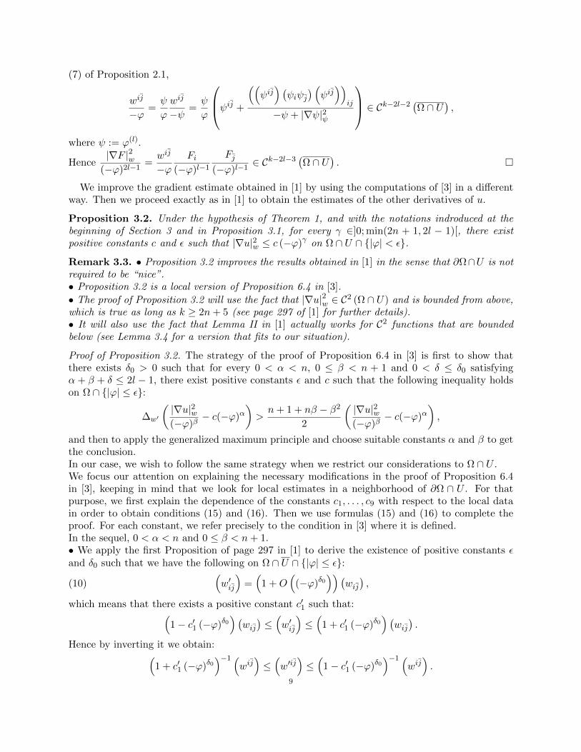
We improve the gradient estimate obtained in [1] by using the computations of [3] in a differentway. Then we proceed exactly as in [1] to obtain the estimates of the other derivatives of u.

Proposition 3.2. Under the hypothesis of Theorem 1, and with the notations indroduced at thebeginning of Section 3 and in Proposition 3.1, for every γ ∈]0; min(2n + 1, 2l − 1)[, there existpositive constants c and ε such that |∇u|2w ≤ c (−ϕ)γ on Ω ∩ U ∩ |ϕ| < ε.

Remark 3.3. • Proposition 3.2 improves the results obtained in [1] in the sense that ∂Ω∩U is notrequired to be “nice”.• Proposition 3.2 is a local version of Proposition 6.4 in [3].

• The proof of Proposition 3.2 will use the fact that |∇u|2w ∈ C2 (Ω ∩ U) and is bounded from above,which is true as long as k ≥ 2n+ 5 (see page 297 of [1] for further details).• It will also use the fact that Lemma II in [1] actually works for C2 functions that are boundedbelow (see Lemma 3.4 for a version that fits to our situation).

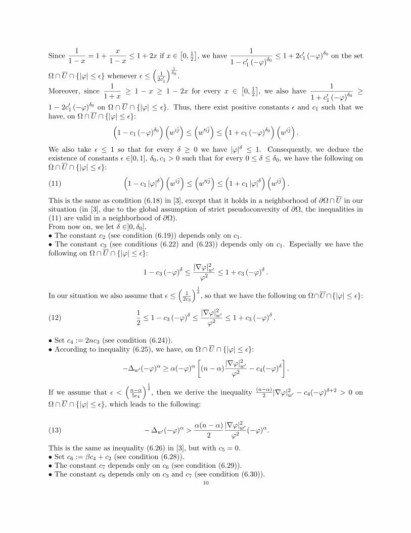
Proof of Proposition 3.2. The strategy of the proof of Proposition 6.4 in [3] is first to show thatthere exists δ0 > 0 such that for every 0 < α < n, 0 ≤ β < n + 1 and 0 < δ ≤ δ0 satisfyingα + β + δ ≤ 2l − 1, there exist positive constants ε and c such that the following inequality holdson Ω ∩ |ϕ| ≤ ε:

∆w′

(|∇u|2w(−ϕ)β

− c(−ϕ)α)>n+ 1 + nβ − β2

2

(|∇u|2w(−ϕ)β

− c(−ϕ)α),

and then to apply the generalized maximum principle and choose suitable constants α and β to getthe conclusion.In our case, we wish to follow the same strategy when we restrict our considerations to Ω ∩ U .We focus our attention on explaining the necessary modifications in the proof of Proposition 6.4in [3], keeping in mind that we look for local estimates in a neighborhood of ∂Ω ∩ U . For thatpurpose, we first explain the dependence of the constants c1, . . . , c9 with respect to the local datain order to obtain conditions (15) and (16). Then we use formulas (15) and (16) to complete theproof. For each constant, we refer precisely to the condition in [3] where it is defined.In the sequel, 0 < α < n and 0 ≤ β < n+ 1.• We apply the first Proposition of page 297 in [1] to derive the existence of positive constants εand δ0 such that we have the following on Ω ∩ U ∩ |ϕ| ≤ ε:

(10)(w′ij

)=(

1 +O(

(−ϕ)δ0)) (

wij),

which means that there exists a positive constant c′1 such that:(1− c′1 (−ϕ)δ0

) (wij)≤(w′ij

)≤(

1 + c′1 (−ϕ)δ0) (wij).

Hence by inverting it we obtain:(1 + c′1 (−ϕ)δ0

)−1 (wij)≤(w′ij

)≤(

1− c′1 (−ϕ)δ0)−1 (

wij).

9

Since1

1− x= 1 +

x

1− x≤ 1 + 2x if x ∈

[0, 1

2

], we have

1

1− c′1 (−ϕ)δ0≤ 1 + 2c′1 (−ϕ)δ0 on the set

Ω ∩ U ∩ |ϕ| ≤ ε whenever ε ≤(

12c′1

) 1δ0 .

Moreover, since1

1 + x≥ 1 − x ≥ 1 − 2x for every x ∈

[0, 1

2

], we also have

1

1 + c′1 (−ϕ)δ0≥

1 − 2c′1 (−ϕ)δ0 on Ω ∩ U ∩ |ϕ| ≤ ε. Thus, there exist positive constants ε and c1 such that wehave, on Ω ∩ U ∩ |ϕ| ≤ ε:(

1− c1 (−ϕ)δ0)(

wij)≤(w′ij

)≤(

1 + c1 (−ϕ)δ0)(

wij).

We also take ε ≤ 1 so that for every δ ≥ 0 we have |ϕ|δ ≤ 1. Consequently, we deduce theexistence of constants ε ∈]0, 1], δ0, c1 > 0 such that for every 0 ≤ δ ≤ δ0, we have the following onΩ ∩ U ∩ |ϕ| ≤ ε:

(11)(

1− c1 |ϕ|δ)(

wij)≤(w′ij

)≤(

1 + c1 |ϕ|δ)(

wij).

This is the same as condition (6.18) in [3], except that it holds in a neighborhood of ∂Ω∩U in oursituation (in [3], due to the global assumption of strict pseudoconvexity of ∂Ω, the inequalities in(11) are valid in a neighborhood of ∂Ω).From now on, we let δ ∈]0, δ0].• The constant c2 (see condition (6.19)) depends only on c1.• The constant c3 (see conditions (6.22) and (6.23)) depends only on c1. Especially we have thefollowing on Ω ∩ U ∩ |ϕ| ≤ ε:

1− c3 (−ϕ)δ ≤|∇ϕ|2w′ϕ2

≤ 1 + c3 (−ϕ)δ .

In our situation we also assume that ε ≤(

12c3

) 1δ, so that we have the following on Ω∩U ∩|ϕ| ≤ ε:

(12)1

2≤ 1− c3 (−ϕ)δ ≤

|∇ϕ|2w′ϕ2

≤ 1 + c3 (−ϕ)δ .

• Set c4 := 2nc3 (see condition (6.24)).• According to inequality (6.25), we have, on Ω ∩ U ∩ |ϕ| ≤ ε:

−∆w′(−ϕ)α ≥ α(−ϕ)α[(n− α)

|∇ϕ|2w′ϕ2

− c4(−ϕ)δ].

If we assume that ε <(n−α5c4

) 1δ, then we derive the inequality (n−α)

2 |∇ϕ|2w′ − c4(−ϕ)δ+2 > 0 on

Ω ∩ U ∩ |ϕ| ≤ ε, which leads to the following:

(13) −∆w′(−ϕ)α >α(n− α)

2

|∇ϕ|2w′ϕ2

(−ϕ)α.

This is the same as inequality (6.26) in [3], but with c5 = 0.• Set c6 := βc4 + c2 (see condition (6.28)).• The constant c7 depends only on c6 (see condition (6.29)).• The constant c8 depends only on c3 and c7 (see condition (6.30)).

10

• If ε <(n+1+nβ−β2

2c8

) 1δ, then we have, on Ω ∩ U ∩ |ϕ| ≤ ε:

n+ 1 + nβ − β2

2− c8(−ϕ)δ > 0,

so that in our case inequality (6.31) becomes the following:

(14) ∆w′

(|∇u|2w(−ϕ)β

)>n+ 1 + nβ − β2

2

|∇u|2w(−ϕ)β

− |∇F |2w(−ϕ)−(δ+β).

Combining (13) and (14), we obtain, on Ω ∩ U ∩ |ϕ| ≤ ε and for every c > 0:

∆w′

(|∇u|2w(−ϕ)β

− c(−ϕ)α)>n+ 1 + nβ − β2

2

|∇u|2w(−ϕ)β

− |∇F |2w(−ϕ)−(δ+β) + cα(n− α)

2

|∇ϕ|2w′ϕ2

(−ϕ)α.

This is exactly the same as inequality (6.31) in [3], but with c9 = 0.• Using condition (9) (Proposition 3.1), we observe that |∇F |2w ≤ c∇(−ϕ)α+δ+β whenever |ϕ| ≤ 1and α+ δ + β ≤ 2l − 1. Therefore, according to (12), the following holds on Ω ∩ U ∩ |ϕ| ≤ ε:

−|∇F |2w(−ϕ)−(δ+β) + cα(n− α)

2

|∇ϕ|2w′ϕ2

(−ϕ)α ≥ −c∇(−ϕ)α + cα(n− α)

2

|∇ϕ|2w′ϕ2

(−ϕ)α

≥(−c∇ + c

α(n− α)

4

)(−ϕ)α.

In particular if we take c > 4c∇α(n−α) the right-hand side is non-negative. This is exactly what is

derived from relation (6.32) in [3] (see the explanation below relation (6.33) in [3]), except that inour case it holds on Ω ∩ U ∩ |ϕ| ≤ ε.

For short, we have proved that there exists δ0 > 0 such that for every 0 < α < n, 0 ≤ β < n+ 1and 0 < δ ≤ δ0 satisfying α+ β + δ ≤ 2l− 1, there exist ε ∈]0, 1] and c > 0 such that the followinginequalities hold on Ω ∩ U ∩ |ϕ| ≤ ε:

(15) ∆w′

(|∇u|2w(−ϕ)β

− c(−ϕ)α)> 0,

(16) ∆w′

(|∇u|2w(−ϕ)β

− c(−ϕ)α)>n+ 1 + nβ − β2

2

(|∇u|2w(−ϕ)β

− c(−ϕ)α).

Inequality (15) implies that the function f := |∇u|2w(−ϕ)β

− c(−ϕ)α cannot achieve its maximum on

Ω∩U ∩|ϕ| ≤ ε, provided it is bounded from above on the set Dε := Ω∩U ∩|ϕ| < ε. Hence wecan find a sequence (zi)i∈N ∈ DN

ε such that limi→+∞

f(z′i)

= supDε

f and dw′ (zi, ∂Dε) −→z→+∞

+∞. Note

that this implies that there exists a positive number R and an integer i0 ∈ N such that for everyi ≥ i0 we have dw′ (zi, ∂Dε) ≥ R.The last step to conclude is to apply the local maximum principle due to J. Bland (see Lemma II in[1]) and use inequation (16). For completeness, we recall the local maximum principle in a versionthat fits our situation:

Lemma 3.4. Let Ω ⊂ Cn be a domain. Assume that there exists a Kahler-Einstein metric inducedby a potential w′ on Ω. Let D ⊂ Ω be a domain. Let f ∈ C2 (D) bounded from above. If there existsa sequence (zi)i∈N ∈ DN such that lim

i→+∞f(z′i)

= supDf and there exists R > 0 such that for every

integer i, dw′ (zi, ∂D) ≥ R, then there exists an other sequence (z′i)i∈N ∈ DN such that

limi→+∞

f(z′i)

= supDf, lim sup

i→+∞∆w′f(z′i) ≤ 0.

11

We apply Lemma 3.4 to f =|∇u|2w(−ϕ)β

− c(−ϕ)α with D = Dε and choose the suitable constants

α, β, δ to conclude. We may argue as follows.

(1) If 2n+ 1 ≤ 2l − 1, we first apply Lemma 3.4 with β = 0, α = n− δ4 and δ ∈ ]0,min (δ0, 4n)[ to

deduce the existence of constants ε ∈]0, 1] and c > 0 for which we have |∇u|2w − c(−ϕ)n−δ4 ≤ 0 on

Ω ∩Dε. Since (−ϕ) < ε ≤ 1 on Ω ∩Dε, this directly implies: |∇u|2w − c(−ϕ)n−δ2 ≤ 0 on Ω ∩Dε.

(2) Hence we may apply Lemma 3.4 with α = β = n − δ2 and δ ∈ ]0,min (δ0, 2n)[ to deduce the

existence of constants ε ∈]0, 1] and c > 0 for which|∇u|2w

(−ϕ)n−δ2

− c(−ϕ)n−δ2 ≤ 0 on Ω ∩Dε. Again,

since (−ϕ) < ε ≤ 1 on Ω ∩Dε, this directly implies: |∇u|2w − c(−ϕ)n+1− δ2 ≤ 0 on Ω ∩Dε.

(3) Hence we may apply once more Lemma 3.4 with β = α+ 1 = n+ 1− δ2 and δ ∈ ]0,min (δ0, 2n)[

to deduce the existence of c, ε > 0 for which|∇u|2w

(−ϕ)n+1− δ2

− c(−ϕ)n−δ2 ≤ 0 on Ω ∩Dε. Finally, we

directly deduce that |∇u|2w ≤ c(−ϕ)2n+1−δ on Ω ∩Dε.

(4) If 2l − 1 < 2n + 1, we can proceed likewise: first taking β = 0, α = min

(n, l − 1

2

)− δ

8

with δ ∈]0,min

(δ0, 8 min

(n, l − 1

2

))[, then considering α = β = min

(n, l − 1

2

)− δ

4with δ ∈]

0,min(δ0, 4 min

(n, l − 1

2

))[, and finally taking α = β = l − 1

2− δ

2with δ ∈ ]0,min (δ0, 2l − 1)[.

In both cases, we obtain the desired conclusion by letting δ tend to 0. Hence the result.

In the rest of Subsection 3.1, we use Proposition 3.2 first to derive the estimates of u of order 0(Proposition 3.5), second to derive estimates of higher order (Proposition 3.7), and finally to obtaina regularity result for ϕe−u (Proposition 3.8).

Proposition 3.5. Under the hypothesis and notations of Proposition 3.2, we have:

(1) For every γ ∈]0,min (2n+ 1, 2l − 1) [, there exist positive constants ε and c such that |∇u| ≤c (−ϕ)

γ2−1 on the set Ω ∩ U ∩ |ϕ| < ε. In particular, if γ > 2, one has u ∈ C1

(Ω ∩ U

).

(2) For every z ∈ ∂Ω ∩ U ,∣∣∣∇e−w′∣∣∣

z6= 0.

(3) For every γ ∈]0,min(2n + 1, 2l − 1)[ there exist positive constants c and ε such that |u| ≤c (−ϕ)

γ2 on Ω ∩ U ∩ |ϕ| < ε.

Remark 3.6. • Observe that relation (10) already gives a control on u. Indeed, by applying Log Det on both sides, using equation (8), and simplifying both sides, we may successively obtain, onΩ ∩ U ∩ |ϕ| ≤ ε:

e(n+1)u−FDet(wij)

=(

1 +O(|ϕ|δ0

))nDet

(wij),

u =n

n+ 1Log

(1 +O

(|ϕ|δ0

))+

F

n+ 1.

Thus, part (3) of Proposition 3.5 only improves the exponent δ0.• Part (3) of Proposition 3.5 is exactly as in [1], the only difference being that we have it forevery γ ∈ ]0,min (2n+ 1, 2l − 1)[. We prove it a slightly different way by first proving part (1) ofProposition 3.5.

Proof of Proposition 3.5. (1) We apply Proposition 3.2, and use Proposition 1.5 with ψ = ηϕ,g = w and U replaced with U ∩ |ϕ| < ε. With notations of Propositions 3.2 and 1.5, we have

12

cλ > 0. Moreover we know that −ψ + |∇ψ|2ψ,

(1η

)2∈ C

(U)

and are positive functions. Hence they

are bounded from above, so that there exist positive constants M1,M2 such that −ψ+ |∇ψ|2ψ ≤M1

and(

1η

)2≤M2 on U . Thus, we have the following on Ω ∩ U :

|∇u|2 ≤ 1

λ

−ψ + |∇ψ|2ψψ2

|∇u|2g ≤c

λ(−ψ + |∇ψ|2ψ)

(ϕ

ψ

)2

(−ϕ)γ−2 ,

=c

λ(−ψ + |∇ψ|2ψ)

(1

η

)2

(−ϕ)γ−2 ,

≤ c

λM1M2 (−ϕ)γ−2 .

Therefore we obtain the conclusion by setting c′ =√

cλM1M2. Especially, if γ > 2, then all

the derivatives of u of order 1 extend continuously to Ω ∩ U (and equal 0 on ∂Ω ∩ U), henceu ∈ C1

(Ω ∩ U

).

(2) To prove part (2) of Proposition 3.5, we let l = n+1. Then by construction e−w′

= −ϕ(n+1)e−u.Moreover, according to point (1) of Proposition 2.1 and to point (1) of Proposition 3.5, we have

ϕ(n+1), u ∈ C1(Ω ∩ U

). Thus e−w

′ ∈ C1(Ω ∩ U

)so that we can differenciate in Ω ∩ U and let z

tend to any point in ∂Ω ∩ U to deduce

limz→∂Ω∩U

∣∣∣∇e−w′∣∣∣z

= limz→∂Ω∩U

∣∣∣∇ϕ(n+1)∣∣∣z6= 0,

because of points (2), (3) of Proposition 2.1.(3) Fix γ ∈ ]0,min (2n+ 1, 2l − 1)[.Let z ∈ U ∩ |ϕ| < ε. Let z0 ∈ ∂Ω ∩ U ∩ |ϕ| < ε such that d(z, ∂Ω) = |z − z0| =: s. Set−→v := z − z0. Define the following function:

f : [0, 1] −→ Rt 7−→ u (z0 + t−→v ) .

According to point (1) of Proposition 3.5 we have f ∈ C1 ([0, s]). Moreover, by the Cauchy-Schwarzinequality we have |f ′(t)| ≤ |∇u|z0+t−→v |

−→v | = s |∇u|z0+t−→v . From point (1) of Remark 3.6 we alsohave u(z0) = 0. Using the fundamental theorem of calculus we deduce:

|u(z)| = |f(1)− f(0)| =∣∣∣∣∫ 1

0f ′(t) dt

∣∣∣∣ ,≤ s

∫ 1

0|∇u|z0+t−→v dt,

≤ cs∫ 1

0(−ϕ (z0 + t−→v ))

γ2−1

dt,

≤ cs

inf [0,1] h′(t)

∫ 1

0h′(t) (h(t))

γ2−1 dt,

=2cs

γ inf [0,1] h′(t)

∫ 1

0

(hγ2

)′(t) dt,

=2cs

γ inf [0,1] h′(t)(−ϕ(z))

γ2 ,

≤ 2cs

γ inf [0,1] h′(t),

13

where h := −ϕ (z0 + ·−→v ) ∈ C1 ([0, 1]). According to point (3) of Proposition 2.1 we have inf[0,1]

h′ > 0.

Hence the result.

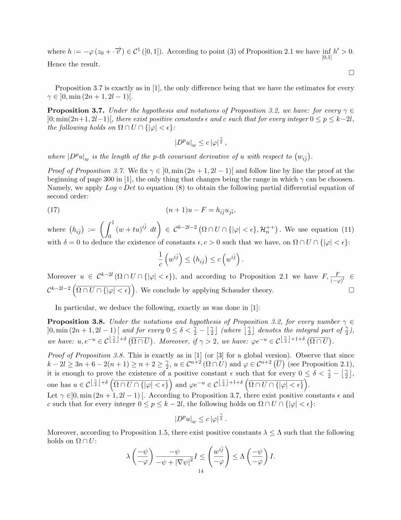
Proposition 3.7 is exactly as in [1], the only difference being that we have the estimates for everyγ ∈ ]0,min (2n+ 1, 2l − 1)[.

Proposition 3.7. Under the hypothesis and notations of Proposition 3.2, we have: for every γ ∈]0; min(2n+1, 2l−1)[, there exist positive constants ε and c such that for every integer 0 ≤ p ≤ k−2l,the following holds on Ω ∩ U ∩ |ϕ| < ε:

|Dpu|w ≤ c |ϕ|γ2 ,

where |Dpu|w is the length of the p-th covariant derivative of u with respect to(wij).

Proof of Proposition 3.7. We fix γ ∈ ]0,min (2n+ 1, 2l − 1)[ and follow line by line the proof at thebeginning of page 300 in [1], the only thing that changes being the range in which γ can be choosen.Namely, we apply Log Det to equation (8) to obtain the following partial differential equation ofsecond order:

(17) (n+ 1)u− F = hijuji,

where(hij)

:=

(∫ 1

0(w + tu)ij dt

)∈ Ck−2l−2

(Ω ∩ U ∩ |ϕ| < ε,H++

n

). We use equation (11)

with δ = 0 to deduce the existence of constants ε, c > 0 such that we have, on Ω ∩ U ∩ |ϕ| < ε:1

c

(wij)≤(hij)≤ c

(wij).

Moreover u ∈ Ck−2l (Ω ∩ U ∩ |ϕ| < ε), and according to Proposition 2.1 we have F, F(−ϕ)l

∈

Ck−2l−2(

Ω ∩ U ∩ |ϕ| < ε)

. We conclude by applying Schauder theory.

In particular, we deduce the following, exactly as was done in [1]:

Proposition 3.8. Under the notations and hypothesis of Proposition 3.2, for every number γ ∈]0,min (2n+ 1, 2l − 1) [ and for every 0 ≤ δ < γ

2 −⌊γ

2

⌋(where

⌊γ2

⌋denotes the integral part of γ

2 ),

we have: u, e−u ∈ Cbγ2 c+δ (Ω ∩ U). Moreover, if γ > 2, we have: ϕe−u ∈ Cb

γ2 c+1+δ

(Ω ∩ U

).

Proof of Proposition 3.8. This is exactly as in [1] (or [3] for a global version). Observe that sincek − 2l ≥ 3n+ 6− 2(n+ 1) ≥ n+ 2 ≥ γ

2 , u ∈ Cn+2 (Ω ∩ U) and ϕ ∈ Cn+2(U)

(see Proposition 2.1),

it is enough to prove the existence of a positive constant ε such that for every 0 ≤ δ < γ2 −

⌊γ2

⌋,

one has u ∈ Cbγ2 c+δ

(Ω ∩ U ∩ |ϕ| < ε

)and ϕe−u ∈ Cb

γ2 c+1+δ

(Ω ∩ U ∩ |ϕ| < ε

).

Let γ ∈]0,min (2n+ 1, 2l − 1) [. According to Proposition 3.7, there exist positive constants ε andc such that for every integer 0 ≤ p ≤ k − 2l, the following holds on Ω ∩ U ∩ |ϕ| < ε:

|Dpu|w ≤ c |ϕ|γ2 .

Moreover, according to Proposition 1.5, there exist positive constants λ ≤ Λ such that the followingholds on Ω ∩ U :

λ

(−ψ−ϕ

)−ψ

−ψ + |∇ψ|2I ≤

(wij

−ϕ

)≤ Λ

(−ψ−ϕ

)I.

14

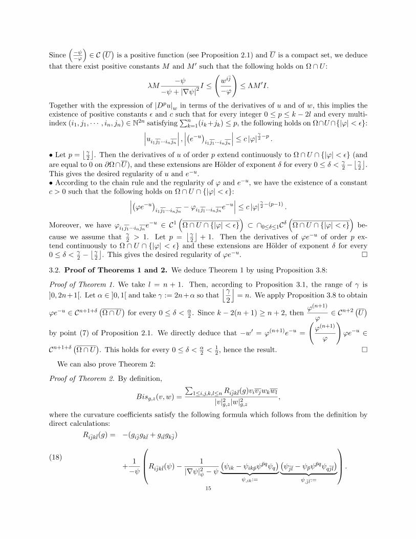
Since(−ψ−ϕ

)∈ C

(U)

is a positive function (see Proposition 2.1) and U is a compact set, we deduce

that there exist positive constants M and M ′ such that the following holds on Ω ∩ U :

λM−ψ

−ψ + |∇ψ|2I ≤

(wij

−ϕ

)≤ ΛM ′I.

Together with the expression of |Dpu|w in terms of the derivatives of u and of w, this implies theexistence of positive constants ε and c such that for every integer 0 ≤ p ≤ k − 2l and every multi-index (i1, j1, · · · , in, jn) ∈ N2n satisfying

∑nk=1(ik+jk) ≤ p, the following holds on Ω∩U∩|ϕ| < ε:∣∣∣ui1j1···injn∣∣∣ , ∣∣∣(e−u)i1j1···injn∣∣∣ ≤ c |ϕ| γ2−p .

• Let p =⌊γ

2

⌋. Then the derivatives of u of order p extend continuously to Ω ∩ U ∩ |ϕ| < ε (and

are equal to 0 on ∂Ω∩U), and these extensions are Holder of exponent δ for every 0 ≤ δ < γ2 −⌊γ

2

⌋.

This gives the desired regularity of u and e−u.• According to the chain rule and the regularity of ϕ and e−u, we have the existence of a constantc > 0 such that the following holds on Ω ∩ U ∩ |ϕ| < ε:∣∣∣(ϕe−u)i1j1···injn − ϕi1j1···injne−u∣∣∣ ≤ c |ϕ| γ2−(p−1) .

Moreover, we have ϕi1j1···injne−u ∈ C1

(Ω ∩ U ∩ |ϕ| < ε

)⊂ ∩0≤δ≤1Cδ

(Ω ∩ U ∩ |ϕ| < ε

)be-

cause we assume that γ2 > 1. Let p =

⌊γ2

⌋+ 1. Then the derivatives of ϕe−u of order p ex-

tend continuously to Ω ∩ U ∩ |ϕ| < ε and these extensions are Holder of exponent δ for every0 ≤ δ < γ

2 −⌊γ

2

⌋. This gives the desired regularity of ϕe−u.

3.2. Proof of Theorems 1 and 2. We deduce Theorem 1 by using Proposition 3.8:

Proof of Theorem 1. We take l = n + 1. Then, according to Proposition 3.1, the range of γ is

]0, 2n+1[. Let α ∈ ]0, 1[ and take γ := 2n+α so that⌊γ

2

⌋= n. We apply Proposition 3.8 to obtain

ϕe−u ∈ Cn+1+δ(Ω ∩ U

)for every 0 ≤ δ < α

2 . Since k − 2(n+ 1) ≥ n+ 2, thenϕ(n+1)

ϕ∈ Cn+2

(U)

by point (7) of Proposition 2.1. We directly deduce that −w′ = ϕ(n+1)e−u =

(ϕ(n+1)

ϕ

)ϕe−u ∈

Cn+1+δ(Ω ∩ U

). This holds for every 0 ≤ δ < α

2 <12 , hence the result.

We can also prove Theorem 2:

Proof of Theorem 2. By definition,

Bisg,z(v, w) =

∑1≤i,j,k,l≤nRijkl(g)vivjwkwl

|v|2g,z|w|2g,z,

where the curvature coefficients satisfy the following formula which follows from the definition bydirect calculations:

(18)

Rijkl(g) = −(gijgkl + gilgkj)

+1

−ψ

Rijkl(ψ)− 1

|∇ψ|2ψ − ψ(ψik − ψikpψpqψq

)︸ ︷︷ ︸ψ,ik:=

(ψj l − ψpψpqψqjl

)︸ ︷︷ ︸ψ,jl:=

.

15

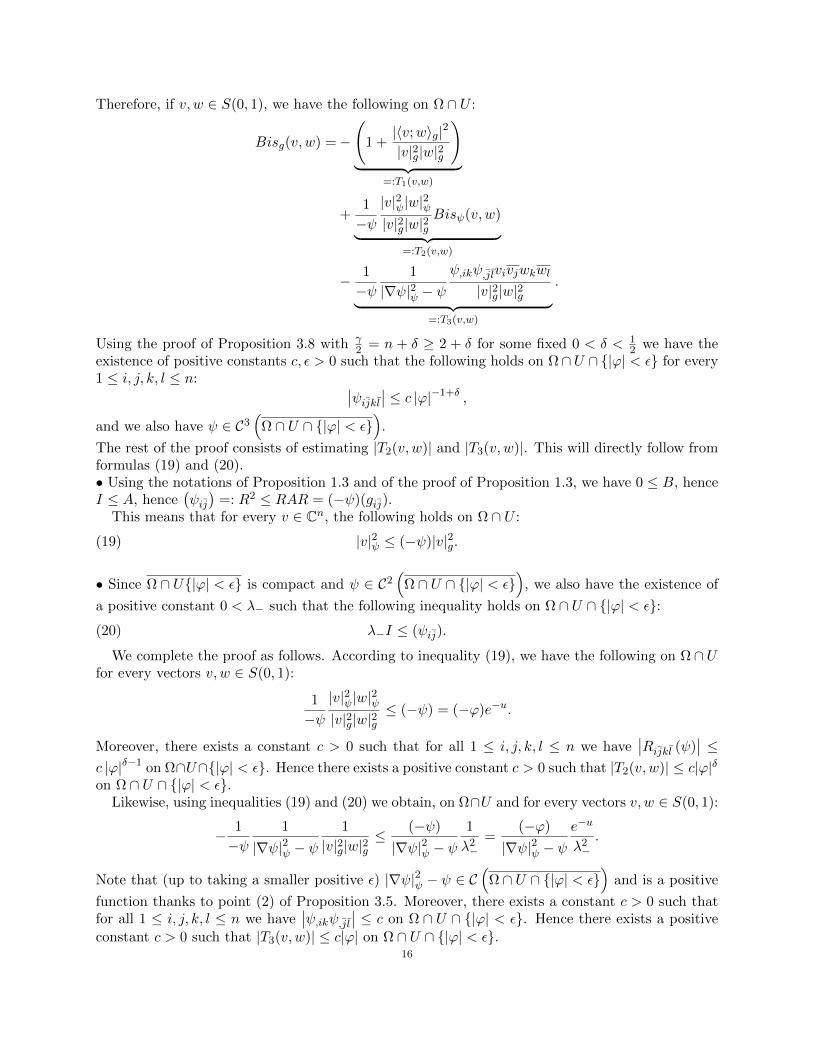
Therefore, if v, w ∈ S(0, 1), we have the following on Ω ∩ U :

Bisg(v, w) =−

(1 +|〈v;w〉g|2

|v|2g|w|2g

)︸ ︷︷ ︸

=:T1(v,w)

+1

−ψ|v|2ψ|w|2ψ|v|2g|w|2g

Bisψ(v, w)︸ ︷︷ ︸=:T2(v,w)

− 1

−ψ1

|∇ψ|2ψ − ψψ,ikψ,jlvivjwkwl

|v|2g|w|2g︸ ︷︷ ︸=:T3(v,w)

.

Using the proof of Proposition 3.8 with γ2 = n + δ ≥ 2 + δ for some fixed 0 < δ < 1

2 we have theexistence of positive constants c, ε > 0 such that the following holds on Ω∩U ∩ |ϕ| < ε for every1 ≤ i, j, k, l ≤ n: ∣∣ψijkl∣∣ ≤ c |ϕ|−1+δ ,

and we also have ψ ∈ C3(

Ω ∩ U ∩ |ϕ| < ε)

.

The rest of the proof consists of estimating |T2(v, w)| and |T3(v, w)|. This will directly follow fromformulas (19) and (20).• Using the notations of Proposition 1.3 and of the proof of Proposition 1.3, we have 0 ≤ B, henceI ≤ A, hence

(ψij)

=: R2 ≤ RAR = (−ψ)(gij).This means that for every v ∈ Cn, the following holds on Ω ∩ U :

|v|2ψ ≤ (−ψ)|v|2g.(19)

• Since Ω ∩ U|ϕ| < ε is compact and ψ ∈ C2(

Ω ∩ U ∩ |ϕ| < ε)

, we also have the existence of

a positive constant 0 < λ− such that the following inequality holds on Ω ∩ U ∩ |ϕ| < ε:(20) λ−I ≤ (ψij).

We complete the proof as follows. According to inequality (19), we have the following on Ω ∩ Ufor every vectors v, w ∈ S(0, 1):

1

−ψ|v|2ψ|w|2ψ|v|2g|w|2g

≤ (−ψ) = (−ϕ)e−u.

Moreover, there exists a constant c > 0 such that for all 1 ≤ i, j, k, l ≤ n we have∣∣Rijkl (ψ)

∣∣ ≤c |ϕ|δ−1 on Ω∩U∩|ϕ| < ε. Hence there exists a positive constant c > 0 such that |T2(v, w)| ≤ c|ϕ|δon Ω ∩ U ∩ |ϕ| < ε.

Likewise, using inequalities (19) and (20) we obtain, on Ω∩U and for every vectors v, w ∈ S(0, 1):

− 1

−ψ1

|∇ψ|2ψ − ψ1

|v|2g|w|2g≤ (−ψ)

|∇ψ|2ψ − ψ1

λ2−

=(−ϕ)

|∇ψ|2ψ − ψe−u

λ2−.

Note that (up to taking a smaller positive ε) |∇ψ|2ψ − ψ ∈ C(

Ω ∩ U ∩ |ϕ| < ε)

and is a positive

function thanks to point (2) of Proposition 3.5. Moreover, there exists a constant c > 0 such thatfor all 1 ≤ i, j, k, l ≤ n we have

∣∣ψ,ikψ,jl∣∣ ≤ c on Ω ∩ U ∩ |ϕ| < ε. Hence there exists a positive

constant c > 0 such that |T3(v, w)| ≤ c|ϕ| on Ω ∩ U ∩ |ϕ| < ε.16

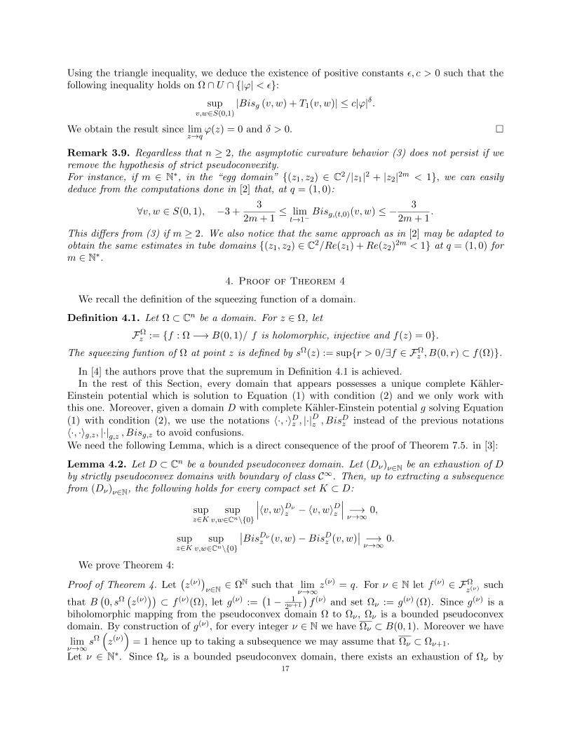
Using the triangle inequality, we deduce the existence of positive constants ε, c > 0 such that thefollowing inequality holds on Ω ∩ U ∩ |ϕ| < ε:

supv,w∈S(0,1)

|Bisg (v, w) + T1(v, w)| ≤ c|ϕ|δ.

We obtain the result since limz→q

ϕ(z) = 0 and δ > 0.

Remark 3.9. Regardless that n ≥ 2, the asymptotic curvature behavior (3) does not persist if weremove the hypothesis of strict pseudoconvexity.For instance, if m ∈ N∗, in the “egg domain” (z1, z2) ∈ C2/|z1|2 + |z2|2m < 1, we can easilydeduce from the computations done in [2] that, at q = (1, 0):

∀v, w ∈ S(0, 1), −3 +3

2m+ 1≤ lim

t→1−Bisg,(t,0)(v, w) ≤ − 3

2m+ 1.

This differs from (3) if m ≥ 2. We also notice that the same approach as in [2] may be adapted toobtain the same estimates in tube domains (z1, z2) ∈ C2/Re(z1) +Re(z2)2m < 1 at q = (1, 0) form ∈ N∗.

4. Proof of Theorem 4

We recall the definition of the squeezing function of a domain.

Definition 4.1. Let Ω ⊂ Cn be a domain. For z ∈ Ω, let

FΩz := f : Ω −→ B(0, 1)/ f is holomorphic, injective and f(z) = 0.

The squeezing funtion of Ω at point z is defined by sΩ(z) := supr > 0/∃f ∈ FΩz , B(0, r) ⊂ f(Ω).

In [4] the authors prove that the supremum in Definition 4.1 is achieved.In the rest of this Section, every domain that appears possesses a unique complete Kahler-

Einstein potential which is solution to Equation (1) with condition (2) and we only work withthis one. Moreover, given a domain D with complete Kahler-Einstein potential g solving Equation(1) with condition (2), we use the notations 〈·, ·〉Dz , |·|

Dz , Bis

Dz instead of the previous notations

〈·, ·〉g,z, |·|g,z , Bisg,z to avoid confusions.

We need the following Lemma, which is a direct consequence of the proof of Theorem 7.5. in [3]:

Lemma 4.2. Let D ⊂ Cn be a bounded pseudoconvex domain. Let (Dν)ν∈N be an exhaustion of Dby strictly pseudoconvex domains with boundary of class C∞. Then, up to extracting a subsequencefrom (Dν)ν∈N, the following holds for every compact set K ⊂ D:

supz∈K

supv,w∈Cn\0

∣∣∣〈v, w〉Dνz − 〈v, w〉Dz ∣∣∣ −→ν→∞ 0,

supz∈K

supv,w∈Cn\0

∣∣BisDνz (v, w)−BisDz (v, w)∣∣ −→ν→∞

0.

We prove Theorem 4:

Proof of Theorem 4. Let(z(ν)

)ν∈N ∈ ΩN such that lim

ν→∞z(ν) = q. For ν ∈ N let f (ν) ∈ FΩ

z(ν) such

that B(0, sΩ

(z(ν)

))⊂ f (ν)(Ω), let g(ν) :=

(1− 1

2ν+1

)f (ν) and set Ων := g(ν) (Ω). Since g(ν) is a

biholomorphic mapping from the pseudoconvex domain Ω to Ων , Ων is a bounded pseudoconvexdomain. By construction of g(ν), for every integer ν ∈ N we have Ων ⊂ B(0, 1). Moreover we have

limν→∞

sΩ(z(ν)

)= 1 hence up to taking a subsequence we may assume that Ων ⊂ Ων+1.

Let ν ∈ N∗. Since Ων is a bounded pseudoconvex domain, there exists an exhaustion of Ων by17

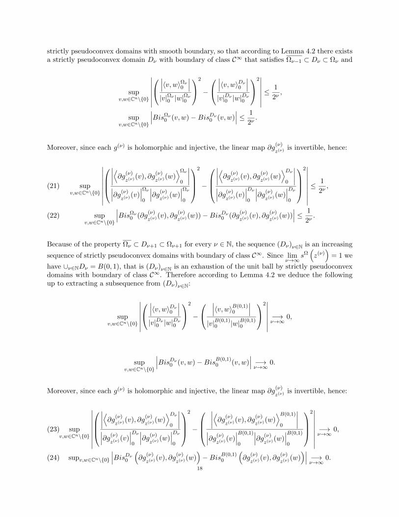
strictly pseudoconvex domains with smooth boundary, so that according to Lemma 4.2 there existsa strictly pseudoconvex domain Dν with boundary of class C∞ that satisfies Ων−1 ⊂ Dν ⊂ Ων and

supv,w∈Cn\0

∣∣∣∣∣∣∣∣∣∣〈v, w〉Ων0

∣∣∣|v|Ων0 |w|

Ων0

2

−

∣∣∣〈v, w〉Dν0

∣∣∣|v|Dν0 |w|

Dν0

2∣∣∣∣∣∣∣ ≤

1

2ν,

supv,w∈Cn\0

∣∣∣BisΩν0 (v, w)−BisDν0 (v, w)

∣∣∣ ≤ 1

2ν.

Moreover, since each g(ν) is holomorphic and injective, the linear map ∂g(ν)

z(ν) is invertible, hence:

supv,w∈Cn\0

∣∣∣∣∣∣∣∣∣∣∣∣∣⟨∂g(ν)

z(ν)(v), ∂g(ν)

z(ν)(w)⟩Ων

0

∣∣∣∣∣∣∣∂g(ν)

z(ν)(v)∣∣∣Ων0

∣∣∣∂g(ν)

z(ν)(w)∣∣∣Ων0

2

−

∣∣∣∣⟨∂g(ν)

z(ν)(v), ∂g(ν)

z(ν)(w)⟩Dν

0

∣∣∣∣∣∣∣∂g(ν)

z(ν)(v)∣∣∣Dν0

∣∣∣∂g(ν)

z(ν)(w)∣∣∣Dν0

2∣∣∣∣∣∣∣∣∣ ≤

1

2ν,(21)

supv,w∈Cn\0

∣∣∣BisΩν0 (∂g

(ν)

z(ν)(v), ∂g(ν)

z(ν)(w))−BisDν0 (∂g(ν)

z(ν)(v), ∂g(ν)

z(ν)(w))∣∣∣ ≤ 1

2ν.(22)

Because of the property Ων ⊂ Dν+1 ⊂ Ων+1 for every ν ∈ N, the sequence (Dν)ν∈N is an increasing

sequence of strictly pseudoconvex domains with boundary of class C∞. Since limν→∞

sΩ(z(ν)

)= 1 we

have ∪ν∈NDν = B(0, 1), that is (Dν)ν∈N is an exhaustion of the unit ball by strictly pseudoconvexdomains with boundary of class C∞. Therefore according to Lemma 4.2 we deduce the followingup to extracting a subsequence from (Dν)ν∈N:

supv,w∈Cn\0

∣∣∣∣∣∣∣∣∣∣〈v, w〉Dν0

∣∣∣|v|Dν0 |w|

Dν0

2

−

∣∣∣〈v, w〉B(0,1)

0

∣∣∣|v|B(0,1)

0 |w|B(0,1)0

2∣∣∣∣∣∣∣ −→ν→∞ 0,

supv,w∈Cn\0

∣∣∣BisDν0 (v, w)−BisB(0,1)0 (v, w)

∣∣∣ −→ν→∞

0.

Moreover, since each g(ν) is holomorphic and injective, the linear map ∂g(ν)

z(ν) is invertible, hence:

supv,w∈Cn\0

∣∣∣∣∣∣∣∣∣∣∣∣∣⟨∂g(ν)

z(ν)(v), ∂g(ν)

z(ν)(w)⟩Dν

0

∣∣∣∣∣∣∣∂g(ν)

z(ν)(v)∣∣∣Dν0

∣∣∣∂g(ν)

z(ν)(w)∣∣∣Dν0

2

−

∣∣∣∣⟨∂g(ν)

z(ν)(v), ∂g(ν)

z(ν)(w)⟩B(0,1)

0

∣∣∣∣∣∣∣∂g(ν)

z(ν)(v)∣∣∣B(0,1)

0

∣∣∣∂g(ν)

z(ν)(w)∣∣∣B(0,1)

0

2∣∣∣∣∣∣∣∣∣ −→ν→∞ 0,(23)

supv,w∈Cn\0

∣∣∣BisDν0

(∂g

(ν)

z(ν)(v), ∂g(ν)

z(ν)(w))−BisB(0,1)

0

(∂g

(ν)

z(ν)(v), ∂g(ν)

z(ν)(w))∣∣∣ −→

ν→∞0.(24)

18

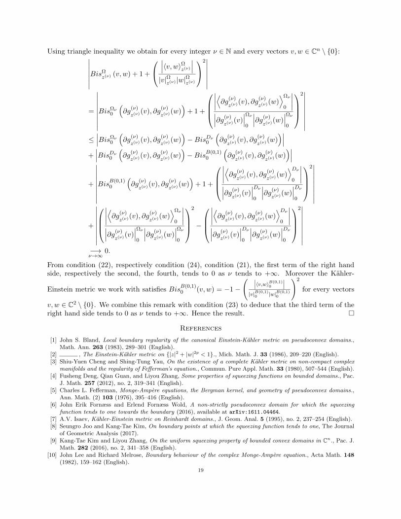
Using triangle inequality we obtain for every integer ν ∈ N and every vectors v, w ∈ Cn \ 0:∣∣∣∣∣∣∣BisΩz(ν) (v, w) + 1 +

∣∣∣〈v, w〉Ωz(ν)

∣∣∣|v|Ωz(ν) |w|Ωz(ν)

2∣∣∣∣∣∣∣

=

∣∣∣∣∣∣∣∣∣BisΩν0

(∂g

(ν)

z(ν)(v), ∂g(ν)

z(ν)(w))

+ 1 +

∣∣∣∣⟨∂g(ν)

z(ν)(v), ∂g(ν)

z(ν)(w)⟩Ων

0

∣∣∣∣∣∣∣∂g(ν)

z(ν)(v)∣∣∣Ων0

∣∣∣∂g(ν)

z(ν)(w)∣∣∣Ων0

2∣∣∣∣∣∣∣∣∣

≤∣∣∣BisΩν

0

(∂g

(ν)

z(ν)(v), ∂g(ν)

z(ν)(w))−BisDν0

(∂g

(ν)

z(ν)(v), ∂g(ν)

z(ν)(w))∣∣∣

+∣∣∣BisDν0

(∂g

(ν)

z(ν)(v), ∂g(ν)

z(ν)(w))−BisB(0,1)

0

(∂g

(ν)

z(ν)(v), ∂g(ν)

z(ν)(w))∣∣∣

+

∣∣∣∣∣∣∣∣∣BisB(0,1)0

(∂g

(ν)

z(ν)(v), ∂g(ν)

z(ν)(w))

+ 1 +

∣∣∣∣⟨∂g(ν)

z(ν)(v), ∂g(ν)

z(ν)(w)⟩Dν

0

∣∣∣∣∣∣∣∂g(ν)

z(ν)(v)∣∣∣Dν0

∣∣∣∂g(ν)

z(ν)(w)∣∣∣Dν0

2∣∣∣∣∣∣∣∣∣

+

∣∣∣∣∣∣∣∣∣∣∣∣∣⟨∂g(ν)

z(ν)(v), ∂g(ν)

z(ν)(w)⟩Ων

0

∣∣∣∣∣∣∣∂g(ν)

z(ν)(v)∣∣∣Ων0

∣∣∣∂g(ν)

z(ν)(w)∣∣∣Ων0

2

−

∣∣∣∣⟨∂g(ν)

z(ν)(v), ∂g(ν)

z(ν)(w)⟩Dν

0

∣∣∣∣∣∣∣∂g(ν)

z(ν)(v)∣∣∣Dν0

∣∣∣∂g(ν)

z(ν)(w)∣∣∣Dν0

2∣∣∣∣∣∣∣∣∣

−→ν→∞

0.

From condition (22), respectively condition (24), condition (21), the first term of the right handside, respectively the second, the fourth, tends to 0 as ν tends to +∞. Moreover the Kahler-

Einstein metric we work with satisfies BisB(0,1)0 (v, w) = −1−

( ∣∣∣〈v,w〉B(0,1)0

∣∣∣|v|B(0,1)

0 |w|B(0,1)0

)2

for every vectors

v, w ∈ C2 \ 0. We combine this remark with condition (23) to deduce that the third term of theright hand side tends to 0 as ν tends to +∞. Hence the result.

References

[1] John S. Bland, Local boundary regularity of the canonical Einstein-Kahler metric on pseudoconvex domains.,Math. Ann. 263 (1983), 289–301 (English).

[2] , The Einstein-Kahler metric on |z|2 + |w|2p < 1., Mich. Math. J. 33 (1986), 209–220 (English).[3] Shiu-Yuen Cheng and Shing-Tung Yau, On the existence of a complete Kahler metric on non-compact complex

manifolds and the regularity of Fefferman’s equation., Commun. Pure Appl. Math. 33 (1980), 507–544 (English).[4] Fusheng Deng, Qian Guan, and Liyou Zhang, Some properties of squeezing functions on bounded domains., Pac.

J. Math. 257 (2012), no. 2, 319–341 (English).[5] Charles L. Fefferman, Monge-Ampere equations, the Bergman kernel, and geometry of pseudoconvex domains.,

Ann. Math. (2) 103 (1976), 395–416 (English).[6] John Erik Fornæss and Erlend Fornæss Wold, A non-strictly pseudoconvex domain for which the squeezing

function tends to one towards the boundary (2016), available at arXiv:1611.04464.[7] A.V. Isaev, Kahler-Einstein metric on Reinhardt domains., J. Geom. Anal. 5 (1995), no. 2, 237–254 (English).[8] Seungro Joo and Kang-Tae Kim, On boundary points at which the squeezing function tends to one, The Journal

of Geometric Analysis (2017).[9] Kang-Tae Kim and Liyou Zhang, On the uniform squeezing property of bounded convex domains in Cn., Pac. J.

Math. 282 (2016), no. 2, 341–358 (English).[10] John Lee and Richard Melrose, Boundary behaviour of the complex Monge-Ampere equation., Acta Math. 148

(1982), 159–162 (English).

19

[11] Ngaiming Mok and Shing-Tung Yau, Completeness of the Kahler-Einstein metric on bounded domains and thecharacterization of domains of holomorphy by curvature conditions., 1983 (English).

[12] Sai-Kee Yeung, Geometry of domains with the uniform squeezing property., Adv. Math. 221 (2009), no. 2, 547–569 (English).

E-mail address: Sebastien.Gontard@univ-grenoble-alpes.fr

Univ. Grenoble Alpes, CNRS, IF, 38000 Grenoble, France

20