warping the kähler potential of f theory/iib ﬂux ... · warping the kähler potential of...

Galileo Galilei

DIPARTIMENTO DI FISICAE ASTRONOMIA

DAF

a

Luca Martucci

Physics and Geometryof F-theory 2015,

Munich, February 23-26, 2015

Warping the Kähler potential of F-theory/IIB flux compactifications

based on: 1411.26230902.4031hep-th/0703129 with P. Koerber

University of Padova

Wflux

=

Z

X⌦ ^G

3

moduli stabilization

FLUXES7-branes

Flux compactifications and warping

SUSY breaking

warping! X

[Gukov-Vafa-Witten]

[Grana-Polchinski, Gubser, Giddings-Kachru-Polchinski]

ds210 = e2A(y)ds24 + e�2A(y)ds2XD3 +O3-planes

FLUXES

D3 +O3-planes

7-branes


X

Wflux

=

Z

X⌦ ^G

3

moduli stabilizationSUSY breakingwarping!

eAmin

<< eAbulk

[Gukov-Vafa-Witten]


[Klebanov-Strassler]

ds210 = e2A(y)ds24 + e�2A(y)ds2X

FLUXES7-branes


X

Wflux

=

Z

X⌦ ^G

3

moduli stabilizationSUSY breakingwarping!

eAmin

<< eAbulk

D3—“de Sitter uplift”(not further considered in this talk)

[Gukov-Vafa-Witten]


[KKL(MM)T,…]

ds210 = e2A(y)ds24 + e�2A(y)ds2XD3 +O3-planes

Question addressed here

How does the warping enter the 4D EFT ?

However, the Kähler potential is expected to be modified

K0ks = �2 log

Z

XJ ^ J ^ J

modified?

The superpotential is insensitive to the warping

In particular, how is

see also:

[Grimm-Louis, Jockers-Louis, Denef, Grimm]

[DeWolfe-Giddings, Maharana-Giddings, Koerber-LM, Marchesano-McGuirk-Shiu, LM, …]

[Frey-Torroba-Underwood-Douglas, Chen-Nakayama-Shiu, Frey-Roberts, … ]

Superconformal symmetry

The 10D metric ds210 = e2Ads24 + e�2Ads2X

is invariant under rescaling:

ds2X ! e2!ds2X

ds24 ! e�2!ds24

e2A ! e2!e2A




ds2X ! e2!ds2X

ds24 ! e�2!ds24

e2A ! e2!e2A

Dynamical ansatz + SUSY 4D local superconformal symmetry

see e.g. [Kallosh-Kofman-Linde-Van Proeyen]

L4D =

Zd4✓N (�, �) = N (�, �)R4 +NIJrµ�

Irµ�J + . . .




ds2X ! e2!ds2X

ds24 ! e�2!ds24

e2A ! e2!e2A

Dynamical ansatz + SUSY 4D local superconformal symmetry

see e.g. [Kallosh-Kofman-Linde-Van Proeyen]

L4D =

Zd4✓N (�, �) = N (�, �)R4 +NIJrµ�

Irµ�J + . . .

conformal Kähler potential

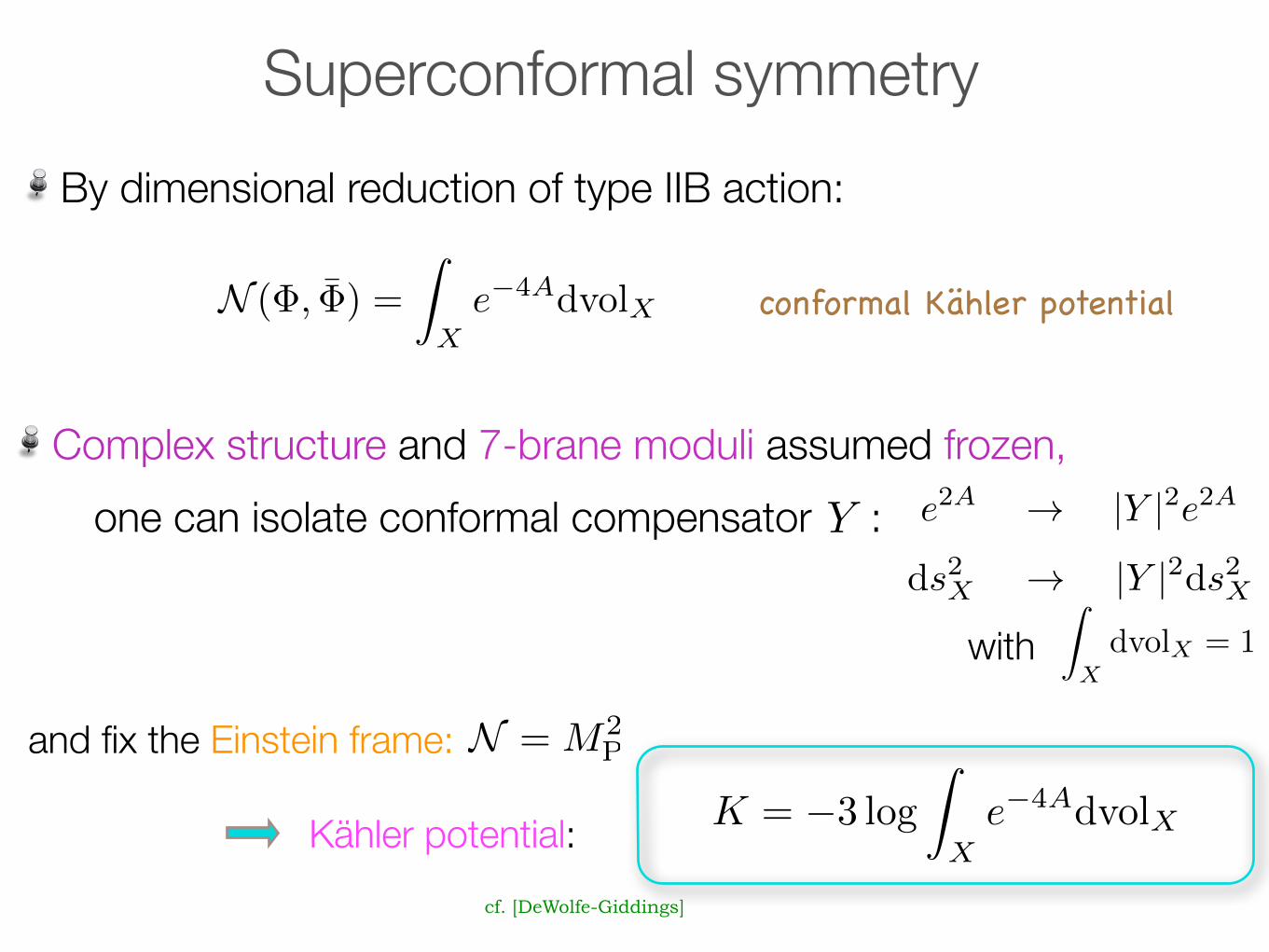
Superconformal symmetry By dimensional reduction of type IIB action:

N (�, ¯�) =

Z

Xe�4A

dvolX conformal Kähler potential


N (�, ¯�) =

Z

Xe�4A


Complex structure and 7-brane moduli assumed frozen,one can isolate conformal compensator : e2A ! |Y |2e2A

ds2X ! |Y |2ds2X

Y

Z

XdvolX = 1with


N (�, ¯�) =

Z

Xe�4A



ds2X ! |Y |2ds2X

Y

Z

XdvolX = 1with

and fix the Einstein frame:

Kähler potential:

N = M2P

K = �3 log

Z

Xe�4A

dvolX

cf. [DeWolfe-Giddings]


N (�, ¯�) =

Z

Xe�4A


rather implicit!


ds2X ! |Y |2ds2X

Y

Z

XdvolX = 1with

and fix the Einstein frame:

Kähler potential:

N = M2P

K = �3 log

Z

Xe�4A

dvolX

cf. [DeWolfe-Giddings]

Universal modulus

�e�4A = ⇤Q6 with Q6 = F3 ^H3 +X

I2D3’s

�6I �1

4

X

O2O3’s

�6O + . . .

The warp factor is determined by the equation:

D3-charge density

universal modulus =

Z

XG(y, y0)Q6(y

0)

e�4A(y) = a+ e�4A0(y)

Universal modulus

By definition: Z

Xe�4A0

dvolX = 0

K = �3 log a

�e�4A = ⇤Q6 with Q6 = F3 ^H3 +X

I2D3’s

�6I �1

4

X

O2O3’s

�6O + . . .


D3-charge density

universal modulus =

Z

XG(y, y0)Q6(y

0)

e�4A(y) = a+ e�4A0(y)

Universal modulus

simple but still implicit!

By definition: Z

Xe�4A0

dvolX = 0

K = �3 log a

�e�4A = ⇤Q6 with Q6 = F3 ^H3 +X

I2D3’s

�6I �1

4

X

O2O3’s

�6O + . . .


D3-charge density

universal modulus =

Z

XG(y, y0)Q6(y

0)

e�4A(y) = a+ e�4A0(y)

Decoding K Sector we focus on:

a

J = va !a

1

3!

Z

XJ ^ J ^ J = 1such that basisH2(M,Z)

h1,1 � 1

harmonic

ZiI I = 1, . . . , nD3

+ axionic partners}good chiral fields

va

D3 positions:

universal modulus:

constrained Kähler moduli :

Decoding K

how to organize them into chiral fields?Question:

Sector we focus on:

a

J = va !a

1

3!

Z


h1,1 � 1

harmonic

ZiI I = 1, . . . , nD3


va

D3 positions:

universal modulus:


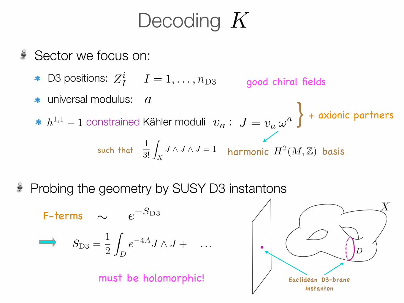
Probing the geometry by SUSY D3 instantons

F-terms ⇠ e�SD3X

Euclidean D3-braneinstanton

DSD3 =

1

2

Z

De�4AJ ^ J + . . .

must be holomorphic!


a

J = va !a

1

3!

Z


h1,1 � 1

harmonic

ZiI I = 1, . . . , nD3


va

D3 positions:

universal modulus:


Natural choice of chiral fields ,

X

Da

such that:

[Da] = !a


a

J = va !a

1

3!

Z


h1,1 � 1

harmonic

ZiI I = 1, . . . , nD3


va

D3 positions:

universal modulus:


⇢a a = 1, . . . , h1,1

Re⇢a =1

2

Z

Da

e�4AJ ^ J +Ref(Z)

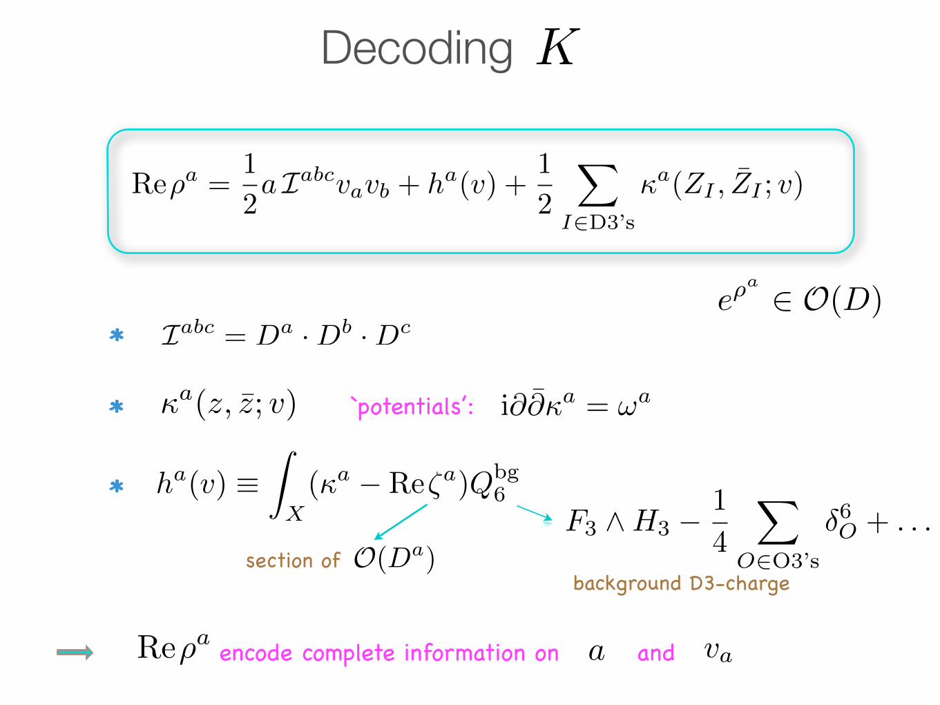
Re⇢a =1

2a Iabcvavb + ha(v) +

1

2

X

I2D3’s

a(ZI , ZI ; v)

a(z, z; v) `potentials’: i@@a = !a

ha(v) ⌘Z

X(a � Re⇣a)Qbg

6

section of O(Da)background D3-charge

Iabc = Da ·Db ·Dce⇢

a 2 O(D)

Decoding K

encode complete information on a and vaRe⇢a

F3 ^H3 �1

4

X

O2O3’s

�6O + . . .

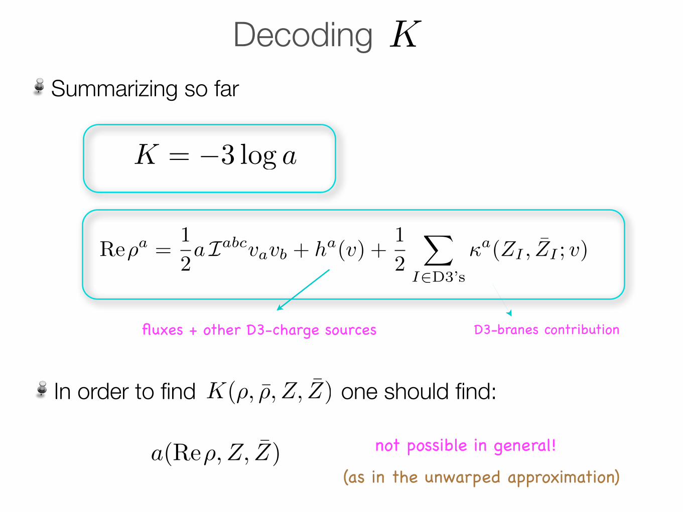
Summarizing so far

Re⇢a =1


1

2

X

I2D3’s

a(ZI , ZI ; v)

K = �3 log a

Decoding K

D3-branes contributionfluxes + other D3-charge sources

Summarizing so far

Re⇢a =1


1

2

X

I2D3’s

a(ZI , ZI ; v)

K = �3 log a

Decoding K

D3-branes contributionfluxes + other D3-charge sources

In order to find one should find:

not possible in general!

(as in the unwarped approximation)

K(⇢, ⇢, Z, Z)

a(Re⇢, Z, Z)

Supersymmetric D3-brane instanton wrapping :

A by-product D

X

Euclidean D3-braneinstanton

D

Wnp ⇠ exp

h� 1

2

Z

De�4AJ ^ J + . . .

i

[Ganor]

[Baumann-Dymarsky-Klebanov-Maldacena-McAllister]

⇠Y

I2D3’s

⇣D(ZI) exp(�⇢)

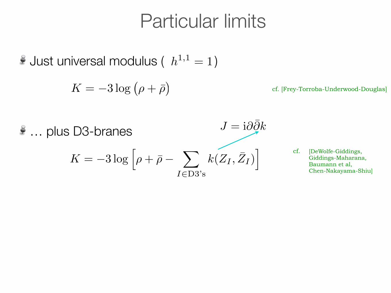
Particular limits

Particular limits

Just universal modulus ( )

cf. [Frey-Torroba-Underwood-Douglas]

h1,1 = 1

K = �3 log

�⇢+ ⇢

�

Particular limits



h1,1 = 1

K = �3 log

�⇢+ ⇢

�

K = �3 log

h⇢+ ⇢�

X

I2D3’s

k(ZI , ¯ZI)

i … plus D3-branes J = i@@k

[DeWolfe-Giddings, Giddings-Maharana, Baumann et al, Chen-Nakayama-Shiu]

cf.

Particular limits



h1,1 = 1

K = �3 log

�⇢+ ⇢

�

K = �3 log

h⇢+ ⇢�

X

I2D3’s

k(ZI , ¯ZI)

i … plus D3-branes J = i@@k

[DeWolfe-Giddings, Giddings-Maharana, Baumann et al, Chen-Nakayama-Shiu]

cf.

Constant warping, no fluxes and weakly fluctuating D3-branes

K = �2 log

�Iabcvavbvc

�va unconstrained

Re⇢a =1

2Iabcvavb �

i

2

X

I2D3’s

!ai|�

iI�

|I

cf. [Graña-Grimm-Jockers-Louis]

Assuming one can approximate

Large moduli limit

Re⇢a � 1

Re⇢a =1

2Iabcvavb

h(v) ⌘Z

X[k(v)� vaRe⇣

a]Qbg6

Qbg6 = F3 ^H3 �

1

4

X

O2O3’s

�6O + . . .

V =1

6Iabcvavbvc va unconstrained

K ' �2 log V +

1

V

hh(v) +

1

2

X

I2D3’s

k(ZI , ¯ZI ; v)i+ . . .


Large moduli limit

Re⇢a � 1

Re⇢a =1

2Iabcvavb

h(v) ⌘Z

X[k(v)� vaRe⇣

a]Qbg6

Qbg6 = F3 ^H3 �

1

4

X

O2O3’s

�6O + . . .

V =1


K ' �2 log V +

1

V

hh(v) +

1

2

X

I2D3’s

k(ZI , ¯ZI ; v)i+ . . .

K0


Large moduli limit

Re⇢a � 1

Re⇢a =1

2Iabcvavb

h(v) ⌘Z

X[k(v)� vaRe⇣

a]Qbg6

Qbg6 = F3 ^H3 �

1

4

X

O2O3’s

�6O + . . .

V =1


⇠ O(V � 23 )

K ' �2 log V +

1

V

hh(v) +

1

2

X

I2D3’s

k(ZI , ¯ZI ; v)i+ . . .

K0

Even though the explicit is not known in general, one can compute the explicit form of the kinetic terms:

Kinetic terms

Gwab ⌘

1

8a2vavb �

1

4a(M�1

w )ab

Lkin = �Gwabrµ⇢

arµ⇢b � 1

2a

X

I

gi|(ZI , ZI)@µZiI@

µZ |I

Mabw ⌘

Z

Xe�4AJ ^ !a ^ !b

K(⇢, ⇢, Z, Z)


Kinetic terms

Gwab ⌘

1

8a2vavb �

1

4a(M�1

w )ab


arµ⇢b � 1

2a

X

I

gi|(ZI , ZI)@µZiI@

µZ |I

Mabw ⌘

Z

Xe�4AJ ^ !a ^ !b

D3-branes kinetic termsmatches what obtained by probe approximation

K(⇢, ⇢, Z, Z)


Kinetic terms

Gwab ⌘

1

8a2vavb �

1

4a(M�1

w )ab


arµ⇢b � 1

2a

X

I

gi|(ZI , ZI)@µZiI@

µZ |I

Mabw ⌘

Z

Xe�4AJ ^ !a ^ !b


K(⇢, ⇢, Z, Z)

warping of Kähler structure moduli space!

(absent if is geometrically formal) Xcf. [Frey-Roberts]


Kinetic terms

Gwab ⌘

1

8a2vavb �

1

4a(M�1

w )ab


arµ⇢b � 1

2a

X

I

gi|(ZI , ZI)@µZiI@

µZ |I

Mabw ⌘

Z

Xe�4AJ ^ !a ^ !b


K(⇢, ⇢, Z, Z)

Furthermore:

is no-scale:KABKAKB = 3

K(⇢, ⇢, Z, Z)

warping of Kähler structure moduli space!

(absent if is geometrically formal) Xcf. [Frey-Roberts]

A simple solvable model

O3-compactification on

⌧ = � = e2⇡i3

G3 ⇠ dz1 ^ dz2 ^ dz3 + dz2 ^ dz3 ^ dz1 + dz3 ^ dz1 ^ dz1

1 =z1z1

Im�2 =

z2z2

Im�3 =

z3z3

Im�

4 =Re(z2z3)

Im�5 =

Re(z3z1)

Im�6 =

Re(z1z2)

Im�

6 moduli + D3’s:

K = � log

hT 1T 2T 3

+ 2T 4T 5T 6 � T 1�T 4

�2 � T 2�T 5

�2 � T 3�T 6

�2i

with

⇢a

no warping of moduli space ⇢a

X = ⇥ ⇥z

i = x

i + �y

i

[Kachru-Schulz-Trivedi]

T a ⌘ Re⇢a � 1

2

X

I

a(ZI , ZI)

Summary

- and D7 axions can be easily incorporated (at weak coupling) B2 C2

At large moduli, warping induced corrections to of order O(V � 23 )K

D3’s automatically incorporated

The Kähler structure moduli space gets warped

Very simple (implicit) Kähler potential K = �3 log a+ flux and D3 dependent chiral coordinates for Kähler structure moduli

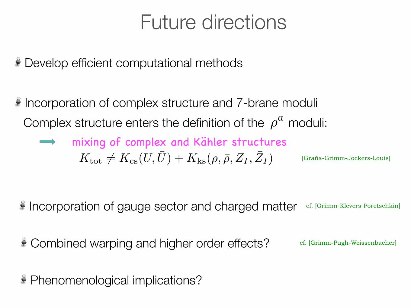
Future directions

Incorporation of gauge sector and charged matter

Phenomenological implications?

Combined warping and higher order effects?

Incorporation of complex structure and 7-brane moduli

cf. [Grimm-Pugh-Weissenbacher]

cf. [Grimm-Klevers-Poretschkin]

mixing of complex and Kähler structures K

tot

6= Kcs

(U, U) +Kks

(⇢, ⇢, ZI , ZI) [Graña-Grimm-Jockers-Louis]

Complex structure enters the definition of the moduli: ⇢a

Develop efficient computational methods

warping the kähler potential of f theory/iib ﬂux ... · warping the kähler potential of...

Documents