on the measure of maximal entropy for finite horizon …

ON THE MEASURE OF MAXIMAL ENTROPY FOR FINITE HORIZONSINAI BILLIARD MAPS

VIVIANE BALADI AND MARK F. DEMERS

Abstract. The Sinai billiard map T on the two-torus, i.e., the periodic Lorentz gas, is adiscontinuous map. Assuming finite horizon, we propose a definition h∗ for the topologicalentropy of T . We prove that h∗ is not smaller than the value given by the variationalprinciple, and that it is equal to the definitions of Bowen using spanning or separating sets.Under a mild condition of sparse recurrence to the singularities, we get more: First, usinga transfer operator acting on a space of anisotropic distributions, we construct an invariantprobability measure µ∗ of maximal entropy for T (i.e., hµ∗ (T ) = h∗), we show that µ∗has full support and is Bernoulli, and we prove that µ∗ is the unique measure of maximalentropy, and that it is different from the smooth invariant measure except if all non grazingperiodic orbits have multiplier equal to h∗. Second, h∗ is equal to the Bowen–Pesin–Pitskeltopological entropy of the restriction of T to a non-compact domain of continuity. Last,applying results of Lima and Matheus, as upgraded by Buzzi, the map T has at least Cenh∗

periodic points of period n for all n ∈ N.

1. Introduction

1.1. Bowen–Margulis Measures and Measures of Maximal Entropy. Half a centuryago1, Margulis [Ma1] proved in his dissertation the following analogue of the prime numbertheorem for the closed geodesics Γ of a compact manifold of strictly negative (not necessarily

Date: Received by the editors August 25, 2018, and, in revised form, August 19, 2019.Electronically published January 6, 2020. https://doi.org/10.1090/jams/939 First published in

Journal of the American Mathematical Society in 2020, published by American Mathematical Society.License or copyright restrictions may apply to redistribution; https://www.ams.org/journal-terms-of-use.

2010 Mathematics Subject Classification. 37D50 (Primary) 37C30; 37B40; 37A25; 46E35; 47B38(Secondary).

Part of this work was carried out during visits of MD to ENS Ulm/IMJ-PRG Paris in 2016 and to IMJ-PRG in 2017 and 2018, during a visit of VB to Fairfield University in 2018, and during the 2018 workshopsNew Developments in Open Dynamical Systems and their Applications in BIRS Banff, and ThermodynamicFormalism in Dynamical Systems in ICMS Edinburgh. We are grateful to F. Ledrappier, C. Matheus, Y.Lima, S. Luzzatto, P.-A. Guihéneuf, G. Forni, B. Fayad, S. Cantat, R. Dujardin, J. Buzzi, P. Bálint, and J.De Simoi for useful comments, to V. Bergelson for encouraging us to establish the Bernoulli property, and toV. Climenhaga for insightful comments which spurred us on to obtain uniqueness. We thank the anonymousreferees for many constructive suggestions. MD was partly supported by NSF grants DMS 1362420 and DMS1800321. VB’s research is supported by the European Research Council (ERC) under the European Union’sHorizon 2020 research and innovation programme (grant agreement No 787304).

1See [Ma2] for the full english text.1

https://doi.org/10.1090/jams/939

https://www.ams.org/journal-terms-of-use

2 VIVIANE BALADI AND MARK F. DEMERS

constant) curvature: Let h > 0 be the topological entropy of the geodesic flow; then,

(1.1) #{Γ such that |Γ| ≤ L} ∼L→∞ehL

hL.

(I.e. limL→∞(hLe−hL#{Γ such that |Γ| ≤ L}) = 1.) The main ingredient in the proof is aninvariant probability measure for the flow, the Margulis (or Bowen–Margulis [Bo3]) measureµtop. This measure — which coincides with volume in constant curvature, but not in general— is mixing (thus ergodic), and it can be written as a local product of its stable and unstableconditionals, where these conditional measures scale by e±ht under the action of the flow.These properties were essential to establish (1.1). The measure µtop enjoys other remarkableproperties, such as equidistribution of closed geodesics. Finally, the measure µtop is theunique measure of maximal entropy of the flow, that is, the unique invariant measure withKolmogorov entropy equal to the topological entropy of the flow.

These results were extended to more general smooth uniformly hyperbolic flows anddiffeomorphisms, using the thermodynamic formalism of Bowen, Ruelle, and Sinai. Inparticular Parry–Pollicott [PaP] obtained a different proof of (1.1) using a dynamical zetafunction. Later, based on Dolgopyat’s [Do1] groundbreaking thesis (proving exponentialmixing for the measure and giving a pole-free vertical strip for a zeta function), exponentialerror terms were obtained [PS1] for the counting asymptotics (1.1) in the case of surfaces or1/4-pinched manifolds. Using [Do1, PS1], Stoyanov [St2] obtained exponential error termsfor the closed orbits of a class of open planar convex billiards, which are smooth hyperbolicflows on their nonwandering set, a compact (fractal) invariant set. We refer to Sharp’s surveyin [Ma2] for more counting results in uniformly hyperbolic dynamics. We just mention herethat, for some Axiom A flows with slower (non-exponential) mixing rates, it is possible [PS2]to get (weaker) error terms, of the form ehL

hL (1 + O(L−δ)), for the asymptotics (1.1), byexploiting relevant operator bounds from [Do2] (corresponding to a resonance free domainfor the transfer operator). This may be relevant for the Sinai billiards considered in thepresent work, as we do not expect them to mix exponentially fast for the measure of maximalentropy without additional assumptions.

Entropy is a fundamental invariant in dynamics and the study of measures of maximalentropy is a topic in its own right [Ka2]. Let us just mention here the discrete-time analogueof the counting theorem (1.1) which has been established in several situations (see also [Ka1]for more general results): Let h > 0 be the topological entropy of uniformly hyperbolic(Axiom A) diffeomorphism T , set FixTm = {x : Tm(x) = x}; then Bowen showed [Bo1]that limm→∞

1m log #FixTm = h. In fact [Bo4], there is a constant C > 0 so that

(1.2) Cehm ≤ #FixTm ≤ C−1ehm , ∀m ≥ 1 .

Uniqueness of the measure of maximal entropy has been extended to some geodesic flowsin non-positive curvature (i.e. weakening the hyperbolicity requirement). The breakthroughresult of Knieper [Kn] for compact rank 1 manifolds has been recently given a new dynamicalproof [B-T] (using Bowen’s ideas as revisited by Climenhaga and Thompson). This iscurrently a very active topic, see e.g. [CKW].

The present paper is devoted to the study of the measure of maximal entropy in a situationwhere uniform hyperbolicity holds, but the dynamics is not smooth: The singular set S±1,

MEASURE OF MAXIMAL ENTROPY FOR SINAI BILLIARD MAPS 3

i.e. those points where the map T (or the flow Φ) or its inverse are not C1, is not empty. Inthis setting, the following integrability condition is crucial:

(1.3)∫| log d(x,S±1)| dµtop <∞ .

Following Lima–Matheus [LM], we shall say that a measure µ satisfying the above integra-bility condition for a map T is T -adapted.

Condition (1.3) is prevalent in the rich literature about measures of maximal entropy formeromorphic maps of a compact Kähler manifold (see the survey [Fr], and e.g. [DDG2]and references therein) such as birational mappings. In this work, we are concerned witha different class of dynamics with singularities: the dispersing billiards introduced by Sinai[S] on the two-torus. A Sinai billiard on the torus is the periodic case of the planar Lorentzgas (1905) model for the motion of a single dilute electron in a metal. The scatterers(corresponding to the atoms of the metal) are assumed to be strictly convex, but they are notnecessarily perfect discs. Such billiards have become foundational models in mathematicalphysics.

The Sinai billiard flow is continuous, but2 not differentiable: the “grazing” orbits (thosewhich are tangent to a scatterer) lead to singularities. Nevertheless, existence of a measureof maximal entropy for the billiard flow is granted, thanks to hyperbolicity. The topologicalentropy has been studied for the billiard flow [BFK]. However, uniqueness of the measure ofmaximal entropy, as well as mixing and the adapted condition (1.3) are not known. Sincethe transfer operator techniques we use are simpler to implement in the discrete-time case,we study in this paper the Sinai billiard map, which is the return map of the single pointparticle to the scatterers.

Sinai billiard maps preserve a smooth invariant measure µSRB which has been studiedextensively: With respect to µSRB, the billiard is uniformly hyperbolic, ergodic, K-mixingand Bernoulli [S, GO, SC, ChH]. The measure µSRB is T -adapted [KS]. Moreover, thismeasure enjoys exponential decay of correlations [Y] and a host of other limit theorems(see e.g. [CM, Chapter 7] or [DZ1]). The billiard has many periodic orbits and thus manyother ergodic invariant measures µ, but there are very few results regarding other invariantmeasures and they apply only to perturbations of µSRB [CWZ, DRZ]. Since the billiard mapis discontinuous, the standard results [W] guaranteeing that the supremum of Kolmogoroventropy is attained and coincides with the topological entropy do not hold. It is naturalto ask whether a measure of maximal entropy exists, and, in the affirmative, whether it isunique, ergodic, and mixing.

Another natural goal is to establish (1.2). Chernov asked (see [Gu, Problems 5 and 6])whether a slightly weaker property than (1.2), namely

limm→∞

1m

log #FixTm = htop ,

holds. (Chernov [Ch1] showed that lim infm→∞ 1m log #FixTm ≥ hµSRB . For a related class

of billiards, Stoyanov [St1] found finite constants C and H so that #FixTm ≤ CeHm for allm ≥ 1.)

2In contrast, open billiards in the plane which satisfy a non-eclipsing condition do not have any singularitieson their nonwandering set, so that they fit in the Axiom A category [St2].


A detailed knowledge of the measure of maximal entropy, and the techniques developedto obtain this information, could potentially allow us not only to establish (1.2) for thebilliard map, but also eventually to prove a prime number asymptotic of the form (1.1) forthe billiard flow. Although lifting a measure of maximal entropy for the map should notdirectly give a measure of maximal entropy for the flow, we believe that the techniques andresults of the present paper will be instrumental in understanding the measure of maximalentropy of the billiard flow.

We list our results in Section 1.2. In a nutshell, for all finite horizon planar Sinai billiardsT satisfying a (mild) condition of “sparse recurrence” to the singular set, we construct ameasure of maximal entropy, we show that it is unique, mixing (even Bernoulli), that it hasfull support, and that it is T -adapted. Our results combined with those of Lima–Matheus[LM] and a very recent preprint of Buzzi [Bu] give C > 0 such that the lower bound in (1.2)holds.

Finally, we mention that our technique for constructing and studying the invariant measure,which uses transfer operators but avoids coding, is reminiscent both of the construction ofMargulis [Ma2] and the techniques of “laminar currents” introduced by Dujardin for birationalmappings [Du] (see also [DDG2]).

1.2. Summary of Main Results. A Sinai billiard table Q on the two-torus T2 is a setQ = T2 \ B, with B = ∪Di=1Bi for some finite number D ≥ 1 of pairwise disjoint closeddomains Bi with C3 boundaries having strictly positive curvature (in particular, the domainsare strictly convex). The sets Bi are called scatterers; see Figure 2 for some common examples.The billiard flow is the motion of a point particle traveling in Q at unit speed and undergoingelastic (i.e., specular) reflections at the boundary of the scatterers. (By definition, at atangential — also called grazing — collision, the reflection does not change the direction ofthe particle.) This is also called a periodic Lorentz gas. As mentioned above, a key feature isthat, although the billiard flow is continuous if one identifies outgoing and incoming angles,the tangential collisions give rise to singularities in the derivative [CM].

We shall be concerned with the associated billiard map T , defined to be the first collisionmap on the boundary of Q. Grazing collisions cause discontinuities in the billiard mapT : M →M . We assume, as in [Y], that the billiard table Q has finite horizon in the sensethat the billiard flow on Q does not have any trajectories making only tangential collisions.

The first step is to find a suitable notion of topological entropy h∗ for the discontinuousmap T .

Let M ′ ⊂ M be the (T -invariant but not compact) set of points whose future and pastorbits are never grazing. By definition, T is continuous on M ′. The (Bowen–Pesin–Pitskel)topological entropy htop(F |Z) can be defined for a map F on an non-compact set of continuityZ (see e.g. [Bo2] and [Pes, §11 and App. II]). Chernov [Ch1] studied the topological entropyfor a class of billiard maps including those of the present paper. In particular, he gave [Ch1,Thm 2.2] a countable symbolic dynamics description of two T -invariant subsets of M ′ offull Lebesgue measure in M ′, expressing their topological entropy in terms of those of theassociated Markov chains. The entropies found there are both bounded above by htop(T |M ′),although Chernov does not prove their equality.


These existing results are not convenient for our purposes, however, since we have nocontrol a priori on the measure of M \M ′. This is why we introduce (Definition 2.1) an adhoc definition h∗ of the topological entropy for the billiard map T on the compact set M .

Our first main result (Theorem 2.3) says that the topological entropies of T defined byspanning sets and separating sets coincide with the topological entropy h∗, that h∗ can also beobtained by using the refinements of partitions of M into maximal connected components onwhich T and T−1 are continuous, and that h∗ ≥ sup{hµ(T ) : µ is a T -invariant Borel probability measure on M}.

To state our other main results, we need to quantify the recurrence to the singular set:Fix an angle ϕ0 close to π/2 and n0 ∈ N. We say that a collision is ϕ0-grazing if its anglewith the normal is larger than ϕ0 in absolute value. Let s0 ∈ (0, 1] be the smallest numbersuch that

any orbit of length n0 has at most s0n0 collisions which are ϕ0-grazing.(1.4)Our sparse recurrence condition is(1.5) there exist n0 and ϕ0 such that h∗ > s0 log 2 .(Due to the finite horizon condition, we can choose ϕ0 and n0 such that s0 < 1. We refer to§2.4 for further discussion of the condition.)

Assuming (1.5), our second main result (Theorem 2.4) is that T admits a unique invariantBorel probability measure µ∗ of maximal entropy h∗ = hµ∗(T ). In addition, µ∗(O) > 0for any open set and µ∗ is3 Bernoulli. Finally, the absolutely continuous invariant measureµSRB may coincide with µ∗ only if all non grazing periodic orbits have the same Lyapunovexponent, equal to h∗. (No dispersing billiards which satisfy this condition are known. Seealso Remark 1.2.)

Our third result is (Theorem 2.5) that h∗ coincides with the Bowen–Pesin–Pitskel entropyhtop(T |M ′) (still assuming (1.5)).

Next, Theorem 2.6 contains a key technical4 estimate on the measures of neighbourhoodsof singularity sets, (2.2), used to prove Theorems 2.4 and 2.5 under the assumption (1.5).Theorem 2.6 also states that µ∗ has no atoms, that it gives zero mass to any stable orunstable manifold and any singularity set, that µ∗ is T -adapted (in the sense of (1.3)), andthat µ∗-almost every x ∈M has stable and unstable manifolds of positive length.

Finally, we obtain a lower bound #FixTm ≥ Ceh∗m on the cardinality of the set ofperiodic orbits (Corollary 2.7 and the comments thereafter) whenever (1.5) holds.

1.3. The Transfer Operator — Organisation of the Paper. Our tool to construct themeasure of maximal entropy is a transfer operator L = Ltop with Lf = f◦T−1

JsT◦T−1 analogousto the transfer operator LSRBf = (f/|DetDT |)◦T−1 which has proved very successful [DZ1]to study the measure µSRB. An important difference is that our transfer operator, Lf , isweighted by an unbounded5 function (1/JsT , where the stable Jacobian JsT may tend tozero near grazing orbits). Using “exact” stable leaves instead of admissible approximate

3Recall that Bernoulli implies K-mixing, which implies strong mixing, which implies ergodic. In practice,we first show K-mixing and then bootstrap to Bernoulli.

4This estimate implies that almost every point approaches the singularity sets more slowly than anyexponential rate (7.9), see e.g. [LM] for an application of such rates of approach.

5The naive idea to introduce a bounded cutoff in the weight does not seem to work.


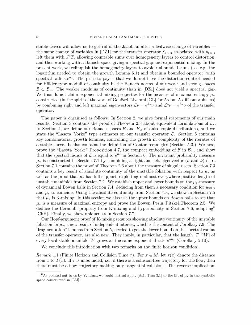
stable leaves will allow us to get rid of the Jacobian after a leafwise change of variables —the same change of variables in [DZ1] for the transfer operator LSRB associated with µSRBleft them with JsT , allowing countable sums over homogeneity layers to control distortion,and thus working with a Banach space giving a spectral gap and exponential mixing. In thepresent work, we relinquish the homogeneity layers to avoid unbounded sums (see e.g. thelogarithm needed to obtain the growth Lemma 5.1) and obtain a bounded operator, withspectral radius eh∗ . The price to pay is that we do not have the distortion control neededfor Hölder type moduli of continuity in the Banach norms of our weak and strong spacesB ⊂ Bw. The weaker modulus of continuity than in [DZ1] does not yield a spectral gap.We thus do not claim exponential mixing properties for the measure of maximal entropy µ∗constructed (in the spirit of the work of Gouëzel–Liverani [GL] for Axiom A diffeomorphisms)by combining right and left maximal eigenvectors Lν = eh∗ν and L∗ν = eh∗ ν of the transferoperator.

The paper is organised as follows: In Section 2, we give formal statements of our mainresults. Section 3 contains the proof of Theorem 2.3 about equivalent formulations of h∗.In Section 4, we define our Banach spaces B and Bw of anisotropic distributions, and westate the “Lasota–Yorke” type estimates on our transfer operator L. Section 5 containskey combinatorial growth lemmas, controlling the growth in complexity of the iterates ofa stable curve. It also contains the definition of Cantor rectangles (Section 5.3.) We nextprove the “Lasota–Yorke” Proposition 4.7, the compact embedding of B in Bw, and showthat the spectral radius of L is equal to eh∗ in Section 6. The invariant probability measureµ∗ is constructed in Section 7.1 by combining a right and left eigenvector (ν and ν) of L.Section 7.1 contains the proof of Theorem 2.6 about the measure of singular sets. Section 7.3contains a key result of absolute continuity of the unstable foliation with respect to µ∗ aswell as the proof that µ∗ has full support, exploiting ν-almost everywhere positive length ofunstable manifolds from Section 7.2. We establish upper and lower bounds on the µ∗-measureof dynamical Bowen balls in Section 7.4, deducing from them a necessary condition for µSRBand µ∗ to coincide. Using the absolute continuity from Section 7.3, we show in Section 7.5that µ∗ is K-mixing. In this section we also use the upper bounds on Bowen balls to see thatµ∗ is a measure of maximal entropy and prove the Bowen–Pesin–Pitskel Theorem 2.5. Wededuce the Bernoulli property from K-mixing and hyperbolicity in Section 7.6, adapting6

[ChH]. Finally, we show uniqueness in Section 7.7.Our Hopf-argument proof of K-mixing requires showing absolute continuity of the unstable

foliation for µ∗, a new result of independent interest, which is the content of Corollary 7.9. The“fragmentation” lemmas from Section 5, needed to get the lower bound on the spectral radiusof the transfer operator, are also new. They imply, in particular, that the length |T−nW | ofevery local stable manifold W grows at the same exponential rate enh∗ (Corollary 5.10).

We conclude this introduction with two remarks on the finite horizon condition.

Remark 1.1 (Finite Horizon and Collision Time τ). For x ∈M , let τ(x) denote the distancefrom x to T (x). If τ is unbounded, i.e., if there is a collision-free trajectory for the flow, thenthere must be a flow trajectory making only tangential collisions. The reverse implication,

6As pointed out to us by Y. Lima, we could instead apply [Sa1, Thm 3.1] to the lift of µ∗ to the symbolicspace constructed in [LM].


however, is not true. Our7 finite horizon assumption therefore implies that τ is bounded onM . Assuming only that τ is bounded is sometimes also called finite horizon [CM]. (If thescatterers Bi are viewed as open, then tangential collisions simply do not occur and the twodefinitions of finite horizon are reconciled.)

Remark 1.2 (Billiard with Infinite Horizon). Chernov [Ch1, §3.4] proved that the topologicalentropy of the Sinai billiard map T restricted to the non compact set M ′ is infinite if thehorizon is not finite, and together with Troubetzkoy [CT] constructed invariant measureswith infinite metric entropy for this map. Since the entropy of the smooth measure µSRB isfinite, the measure µSRB does not maximise entropy for infinite horizon billiards. Chernovconjectured [Ch1, Remark 3.3] that this property holds for more general billiards, in particularfor Sinai billiards with finite horizon.

2. Full Statement of Main Results

In this section, we formulate definitions of topological entropy for the billiard map thatwe shall prove are equivalent before stating formally all main results of this paper.

2.1. Definitions of Topological Entropy h∗ of T on M . We first introduce notation:Adopting the standard coordinates x = (r, ϕ), for T , where r denotes arclength along ∂Biand ϕ is the angle the post-collision trajectory makes with the normal to ∂Bi, the phasespace of the map is the compact metric space M given by the disjoint union of cylinders,

M := ∂Q×[−π2 ,

π

2

]=

D⋃i=1

∂Bi ×[−π2 ,

π

2

].

We denote each connected component ofM byMi = ∂Bi× [−π2 ,

π2 ]. In the coordinates (r, ϕ),

the billiard map T : M →M preserves [CM, §2.12] the smooth invariant measure8 definedby µSRB = (2|∂Q|)−1 cosϕdrdϕ.

We discuss next the discontinuity set of T : Letting S0 = {(r, ϕ) ∈M : ϕ = ±π/2} denotethe set of tangential collisions, then for each nonzero n ∈ N, the set

S±n = ∪ni=0T∓iS0

is the singularity set for T±n. In this notation, the T -invariant (non compact) set M ′ ofcontinuity of T is M ′ = M \ ∪n∈ZSn.

For k, n ≥ 0, letMn−k denote the partition of M \ (S−k ∪ Sn) into its maximal connected

components. Note that all elements ofMn−k are open sets. The cardinality of the setsMn

0will play a key role in the estimates on the transfer operator in Section 4. We formulate thefollowing definition with the idea that the growth rate of elements inMn

−k should define thetopological entropy of T , by analogy with the definition using a generating open cover (forcontinuous maps on compact spaces).

Definition 2.1. h∗ = h∗(T ) := lim supn→∞ 1n log #Mn

0 .

7We shall need the slightly stronger version e.g. in Lemmas 3.4 and 3.5.8All measures in this work are finite Borel measures.


1 2 3 1

2

3 40

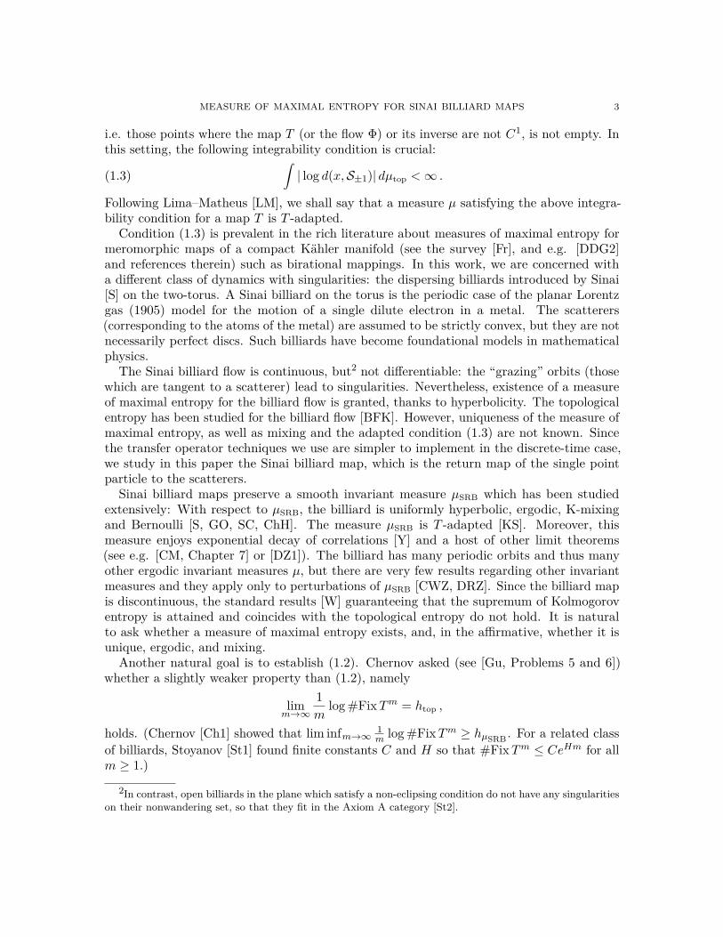
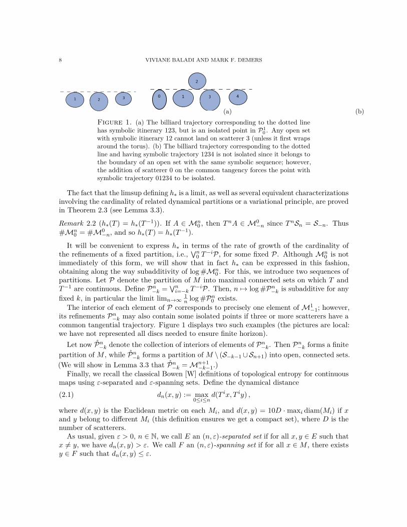
(a) (b)Figure 1. (a) The billiard trajectory corresponding to the dotted linehas symbolic itinerary 123, but is an isolated point in P1

0 . Any open setwith symbolic itinerary 12 cannot land on scatterer 3 (unless it first wrapsaround the torus). (b) The billiard trajectory corresponding to the dottedline and having symbolic trajectory 1234 is not isolated since it belongs tothe boundary of an open set with the same symbolic sequence; however,the addition of scatterer 0 on the common tangency forces the point withsymbolic trajectory 01234 to be isolated.

The fact that the limsup defining h∗ is a limit, as well as several equivalent characterizationsinvolving the cardinality of related dynamical partitions or a variational principle, are provedin Theorem 2.3 (see Lemma 3.3).

Remark 2.2 (h∗(T ) = h∗(T−1)). If A ∈ Mn0 , then TnA ∈ M0

−n since TnSn = S−n. Thus#Mn

0 = #M0−n, and so h∗(T ) = h∗(T−1).

It will be convenient to express h∗ in terms of the rate of growth of the cardinality ofthe refinements of a fixed partition, i.e.,

∨n0 T−iP, for some fixed P. Although Mn

0 is notimmediately of this form, we will show that in fact h∗ can be expressed in this fashion,obtaining along the way subadditivity of log #Mn

0 . For this, we introduce two sequences ofpartitions. Let P denote the partition of M into maximal connected sets on which T andT−1 are continuous. Define Pn−k =

∨ni=−k T

−iP. Then, n 7→ log #Pn−k is subadditive for anyfixed k, in particular the limit limn→∞

1n log #Pn0 exists.

The interior of each element of P corresponds to precisely one element ofM1−1; however,

its refinements Pn−k may also contain some isolated points if three or more scatterers have acommon tangential trajectory. Figure 1 displays two such examples (the pictures are local:we have not represented all discs needed to ensure finite horizon).

Let now Pn−k denote the collection of interiors of elements of Pn−k. Then Pn−k forms a finitepartition of M , while Pn−k forms a partition of M \ (S−k−1 ∪Sn+1) into open, connected sets.(We will show in Lemma 3.3 that Pn−k =Mn+1

−k−1.)Finally, we recall the classical Bowen [W] definitions of topological entropy for continuous

maps using ε-separated and ε-spanning sets. Define the dynamical distance(2.1) dn(x, y) := max

0≤i≤nd(T ix, T iy) ,

where d(x, y) is the Euclidean metric on each Mi, and d(x, y) = 10D ·maxi diam(Mi) if xand y belong to different Mi (this definition ensures we get a compact set), where D is thenumber of scatterers.

As usual, given ε > 0, n ∈ N, we call E an (n, ε)-separated set if for all x, y ∈ E such thatx 6= y, we have dn(x, y) > ε. We call F an (n, ε)-spanning set if for all x ∈M , there existsy ∈ F such that dn(x, y) ≤ ε.


Let rn(ε) denote the maximal cardinality of any (n, ε)-separated set, and let sn(ε) denotethe minimal cardinality of any (n, ε)-spanning set. We recall two related quantities:

hsep = limε→0

lim supn→∞

1n

log rn(ε) , hspan = limε→0

lim supn→∞

1n

log sn(ε) .

Although limn→∞1n log #Pn0 , hsep, and hspan are typically used for continuous maps, our

first main result is that these naively defined quantities for the discontinuous billiard map Tall agree with h∗, and they give an upper bound for the Kolmogorov entropy:

Theorem 2.3 (Topological Entropy of the Billiard). The limsup in Definition 2.1 is a limit,and in fact the sequence log #Mn

0 is subadditive. In addition, we have:(1) h∗ = limn→∞

1n log #Pn0 ;

(2) the sequence 1n log #Pn0 also converges to h∗ as n→∞;

(3) h∗ = hsep and h∗ = hspan;(4) h∗ ≥ sup{hµ(T ) : µ is a T -invariant Borel probability measure on M}.

The above theorem will follow from Lemmas 3.3, 3.4, 3.5, and 3.6.(We shall obtain in Lemma 5.6 a superadditive property for log #Mn

0 .)

2.2. The Measure µ∗ of Maximal Entropy. Our next main result, existence and theBernoulli property of a unique measure of maximal entropy, will be proved in Section 7,using the transfer operator L studied in Section 4.

Theorem 2.4 (Measure of Maximal Entropy for the Billiard). If h∗ > s0 log 2 thenh∗ = max{hµ(T ) : µ is a T -invariant Borel probability measure on M} .

Moreover, there exists a unique T -invariant Borel probability measure µ∗ such that h∗ =hµ∗(T ). In addition, µ∗ is Bernoulli and µ∗(O) > 0 for all open sets O. Finally, if thereexists a non grazing periodic point x of period p such that 1

p log |det(DT−p|Es(x))| 6= h∗ thenµ∗ 6= µSRB.

The above theorem follows from Propositions 7.11, 7.13, and 7.19, Corollary 7.17, andProposition 7.21. (J. De Simoi has told us that [DKL, §4.4] the (possibly empty) set ofplanar billiard tables satisfying a non-eclipsing condition (i.e., open billiards) for which1p log | det(DT−p|Es(x))| = h∗ for all p and all non-grazing p-periodic points x has infinitecodimension.)

The existence of µ∗ with hµ∗(T ) = h∗, together with item (1) of Theorem 2.3 expressingh∗ as a limit involving the refinements of a single partition, will allow us to interpret h∗ asthe Bowen–Pesin–Pitskel topological entropy of T |M ′ in Section 7.5:

Theorem 2.5 (h∗ and Bowen–Pesin–Pitskel Entropy). If h∗ > s0 log 2 then h∗ = htop(T |M ′).

2.3. A Key Estimate on Neighbourhood of Singularities. We call a smooth curve inM a stable curve if its tangent vector at each point lies in the stable cone, and define anunstable curve similarly. As mentioned in Section 1, the sets Sn are the singularity sets forTn, n ∈ Z \ {0}. The set Sn \S0 comprises [CM] a finite union of stable curves for n > 0 anda finite union of unstable curves for n < 0. For any ε > 0 and any set A ⊂M , we denote byNε(A) = {x ∈M | d(x,A) < ε} the ε-neighbourhood of A.


The following key result gives information on the measure of neighbourhoods of thesingularity sets (it is used in the proofs of Theorem 2.4 and, indirectly, Theorem 2.5).

Theorem 2.6 (Measure of Neighbourhoods of Singularity Sets). Assume that h∗ > s0 log 2and let µ∗ be the ergodic measure of maximal entropy constructed in (7.1). The measureµ∗ has no atoms, and for any local stable or unstable manifold W we have µ∗(W ) = 0. Inaddition µ∗(Sn) = 0 for any n ∈ Z.

More precisely, for any γ > 0 so that 2s0γ < eh∗ and n ∈ Z, there exist C and Cn < ∞such that for all ε > 0 and any smooth curve S uniformly transverse to the stable cone,

(2.2) µ∗(Nε(S)) < C

| log ε|γ , µ∗(Nε(Sn)) < Cn| log ε|γ .

Since h∗ > s0 log 2 we may take γ > 1, and we have∫| log d(x,S±1)| dµ∗ <∞ ,

(i.e., µ∗ is T -adapted [LM]), and µ∗-almost every x ∈M has stable and unstable manifoldsof positive length.

Theorem 2.6 follows from Lemma 7.3 and Corollary 7.4.This theorem is especially of interest for γ > 1, since in this case it implies that µ∗-almost

every point does not approach the singularity sets faster than some exponential, see (7.9).In addition, it allows us to give a lower bound on the number of periodic orbits: For m ≥ 1,let FixTm denote the set {x ∈ M | Tm(x) = x}. By [BSC] and [Ch1, Cor 2.4], there existhC ≥ hµSRB(T ) > 0 and C > 0 with #FixTm ≥ CehCm for all m. Our result is that(possibly up to a period p) we can take hC = h∗ if h∗ > s0 log 2:

Corollary 2.7 (Counting Periodic Orbits). If h∗ > s0 log 2 then there exist C > 0 and p ≥ 1such that #FixT pm ≥ Ceh∗pm for all m ≥ 1.

Proof. The corollary follows from the work of Lima–Matheus [LM], which in turn relies onwork of Gurevič [G1, G2] (see the proof of [Sa2, Thm 1.1]). We recall briefly the setup of[LM, Theorem 1.3]: Under assumptions (A1)-(A6), the authors construct for any T -adaptedmeasure µ with positive Lyapunov exponent, a countable Markov partition that allows themto code a full µ-measure set of points. Once this partition has been constructed, [LM,Corollary 1.2] implies the above lower bound on periodic orbits for T with rate given byhµ(T ).

[LM, Theorem 1.3] applies to our measure of maximal entropy µ∗ since it is T -adapted withpositive Lyapunov exponent. In addition, conditions (A1)-(A4) of [LM] are requirements onthe smoothness of the exponential map on the manifold, which are trivially satisfied in oursetting since M is a finite union of cylinders and S±1 is a finite union of curves. Finally,conditions (A5) and (A6) are requirements on the rate at which ‖DT‖ and ‖D2T‖ grow asone approaches S1. These are standard estimates for billiards and in the notation of [LM],if we choose a = 2, then conditions (A5) and (A6) hold, choosing there β = 1/4 and anyb > 1. �

After the first version of our paper was submitted, J. Buzzi [Bu, v2] obtained resultsallowing one to bootstrap from Corollary 2.7 by exploiting the fact that T is topologically


mixing, to show that if h∗ > s0 log 2 then there exists C > 0 so that #FixTm ≥ Ceh∗m forall m ≥ 1 [Bu, Theorem 1.5] .

2.4. On Condition (1.5) of Sparse Recurrence to Singularities. We are not awareof any dispersing billiard on the torus for which the bound h∗ > s0 log 2 from (1.5) fails.Let us start by mentioning that if there are no triple tangencies on the table — a genericcondition — then s0 ≤ 2/3. To discuss this condition further, our starting point is claim (4)of Theorem 2.3, which implies by the Pesin entropy formula [KS],

(2.3) h∗ ≥ hµSRB(T ) =∫

log JuT dµSRB .

Thus it suffices to check χ+µSRB > s0 log 2 in order to verify (1.5), where χ+

µSRB =∫

log JuT dµSRBis the positive Lyapunov exponent of µSRB.

d

(a)

ρ

R

(b)

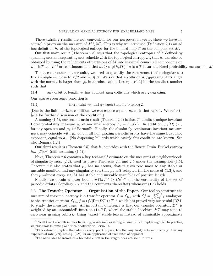
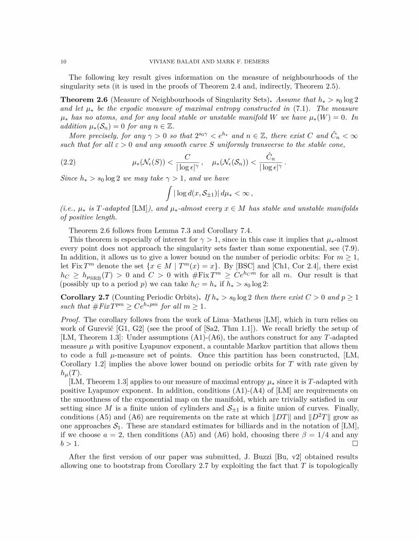
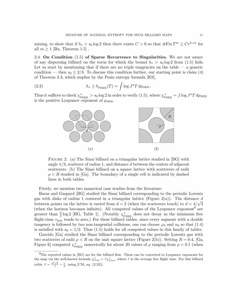
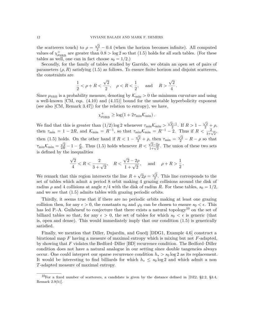
Figure 2. (a) The Sinai billiard on a triangular lattice studied in [BG] withangle π/3, scatterer of radius 1, and distance d between the centers of adjacentscatterers. (b) The Sinai billiard on a square lattice with scatterers of radiiρ < R studied in [Ga]. The boundary of a single cell is indicated by dashedlines in both tables.

Firstly, we mention two numerical case studies from the literature:Baras and Gaspard [BG] studied the Sinai billiard corresponding to the periodic Lorentz

gas with disks of radius 1 centered in a triangular lattice (Figure 2(a)). The distance dbetween points on the lattice is varied from d = 2 (when the scatterers touch) to d = 4/

√3

(when the horizon becomes infinite). All computed values of the Lyapunov exponent9 aregreater than 2

3 log 2 [BG, Table 1]. (Notably χ+µSRB does not decay as the minimum free

flight-time τmin tends to zero.) For these billiard tables, since every segment with a doubletangency is followed by two non-tangential collisions, one can choose ϕ0 and n0 so that (1.4)is satisfied with s0 = 1/2. Thus (1.5) holds for all computed values in this family of tables.

Garrido [Ga] studied the Sinai billiard corresponding to the periodic Lorentz gas withtwo scatterers of radii ρ < R on the unit square lattice (Figure 2(b)). Setting R = 0.4, [Ga,Figure 6] computed χ+

µSRB numerically for about 20 values of ρ ranging from ρ = 0.1 (when

9The reported values in [BG] are for the billiard flow. These can be converted to Lyapunov exponents forthe map via the well-known formula χ+

map = τχ+flow, where τ is the average free flight time. For this billiard

table, τ = d2√34 − π

2 , using [CM, eq. (2.32)].


the scatterers touch) to ρ =√

22 − 0.4 (when the horizon becomes infinite). All computed

values of χ+µSRB are greater than 0.8 > log 2 so that (1.5) holds for all such tables. (For these

tables as well, one can in fact choose s0 = 1/2.)Secondly, for the family of tables studied by Garrido, we obtain an open set of pairs of

parameters (ρ,R) satisfying (1.5) as follows. To ensure finite horizon and disjoint scatterers,the constraints are

12 < ρ+R <

√2

2 , ρ < R <12 , and R >

√2

4 .

Since µSRB is a probability measure, denoting by Kmin > 0 the minimum curvature and usinga well-known [CM, eqs. (4.10) and (4.15)] bound for the unstable hyperbolicity exponent(see also [CM, Remark 3.47]) for the relation to entropy), we have,

χ+µSRB ≥ log(1 + 2τminKmin) .

We find that this is greater than (1/2) log 2 whenever τminKmin >√

2−12 . If R > 1−

√2

2 + ρ,then τmin = 1 − 2R, and Kmin = R−1, so that τminKmin = R−1 − 2. Thus if R < 2

3+√

2 ,

then (1.5) holds. On the other hand if R < 1 −√

22 + ρ, then τmin =

√2

2 − R − ρ so thatτminKmin =

√2

2R − 1− ρR . Thus (1.5) holds whenever R <

√2−2ρ

1+√

2 . The union of these two setsis defined by the inequalities

√2

4 < R <2

3 +√

2, R <

√2− 2ρ

1 +√

2, and ρ+R >

12 .

We remark that this region intersects the line R+√

2ρ =√

22 . This line corresponds to the

set of tables which admit a period 8 orbit making 4 grazing collisions around the disk ofradius ρ and 4 collisions at angle π/4 with the disk of radius R. For these tables, s0 = 1/2,and we see that (1.5) admits tables with grazing periodic orbits.

Thirdly, it seems true that if there are no periodic orbits making at least one grazingcollision then, for any ε > 0, the constants n0 and ϕ0 can be chosen to ensure s0 < ε. Thishas led P.-A. Guihéneuf to conjecture that there exists a natural topology10 on the set ofbilliard tables so that, for any ε > 0, the set of tables for which s0 < ε is generic (thatis, open and dense). This would immediately imply that our condition (1.5) is genericallysatisfied.

Finally, we mention that Diller, Dujardin, and Guedj [DDG1, Example 4.6] construct abirational map F having a measure of maximal entropy which is mixing but not F -adapted,by showing that F violates the Bedford–Diller [BD] recurrence condition. The Bedford–Dillercondition does not have a natural analogue in our setting since double tangencies alwaysoccur. One could interpret our sparse recurrence condition h∗ > s0 log 2 as its replacement.It would be interesting to find billiards for which h∗ ≤ s0 log 2 and which admit a nonT -adapted measure of maximal entropy.

10For a fixed number of scatterers, a candidate is given by the distance defined in [DZ2, §2.2, §3.4,Remark 2.9(b)].


3. Proof of Theorem 2.3 (Equivalent Formulations of h∗)

In this section, we shall prove Theorem 2.3 through Lemmas 3.3, 3.4, 3.5, and 3.6.We first recall some facts about the uniform hyperbolicity of T to introduce notation

which will be used throughout. It is well known [CM] that T is uniformly hyperbolic in thefollowing sense: First, the cones Cu = {(dr, dϕ) ∈ R2 : Kmin ≤ dϕ/dr ≤ Kmax + 1/τmin}and Cs = {(dr, dϕ) ∈ R2 : −Kmin ≥ dϕ/dr ≥ −Kmax − 1/τmin}, are strictly invariant underDT and DT−1, respectively, whenever these derivatives exist. Here, Kmax represent themaximum curvature of the scatterer boundaries and τmax <∞ is the largest free flight timebetween collisions. Second, recalling that Kmin > 0, τmin > 0 denote the minimum curvatureand the minimum free flight time, and setting

Λ := 1 + 2Kminτmin ,

there exists C1 > 0 such that for all n ≥ 0,

(3.1) ‖DTn(x)v‖ ≥ C1Λn‖v‖ , ∀v ∈ Cu , ‖DT−n(x)v‖ ≥ C1Λn‖v‖ , ∀v ∈ Cs ,

for all x for which DTn(x), or respectively DT−n(x), is defined, so that Λ is a lower bound11

on the hyperbolicity constant of the map T .

3.1. Preliminaries. The following lemma provides important information regarding thestructure of the partitions Pn−k, which we will use to make an explicit connection betweenMn−k and Pn−k in Lemma 3.3.

Lemma 3.1. The elements of Pn−k are connected sets for all k ≥ 0 and n ≥ 0.

Proof. The statement is true by definition for P = P00 . We will prove the general statement by

induction on k and n using the fact that Pn+1−k = Pn−k

∨T−1Pn−k, and Pn−k−1 = Pn−k

∨TPn−k.

Fix k, n ≥ 0, and assume the elements of Pn−k are connected sets. Let A1, A2 ∈ Pn−k. IfT−1A1 ∩ A2 is empty or is an isolated point, then it is connected. So suppose T−1A1 ∩ A2has nonempty interior.

Clearly, T−1A1 is connected since T−1 is continuous on elements of Pn−k for all k, n ≥ 0.Notice that the boundary of A1 is comprised of finitely many smooth stable and unstablecurves in S−k ∪Sn, as well as possibly a subset of S0 ([CM, Prop 4.45 and Exercise 4.46], seealso [CM, Fig 4.17]). We shall refer to these as the stable and unstable parts of the boundaryof A1. Similar facts apply to the boundaries of A2 and TA1.

We consider whether a stable part of the boundary of T−1A1 can cross a stable part ofthe boundary of A2, and create two or more connected components of T−1A1 ∩ A2. Callthese two boundary components γ1 and γ2 and notice that such an occurrence would forceγ1 and γ2 to intersect in at least two points.

We claim the following fact: If a stable curve Si ⊂ T−iS0 intersects Sj ⊂ T−jS0 for i < j,then Sj must terminate on Si. This is because T iSi ⊂ S0, while T iSj ⊂ T i−jS0 is still astable curve, terminating on S0. A similar property holds for unstable surves in S−i. andS−j .

11Therefore, hµSRB(T ) =∫

log JuT dµSRB > log Λ and the bound log(1 + 2Kminτmin) > s0 log 2 implies(1.5), as in Section 2.4.


The claim implies that γ1 and γ2 both belong to T−jS0 for some 1 ≤ j ≤ n. But when suchcurves intersect, again, one must terminate on the other (crossing would violate injectivityof T−1).

A similar argument precludes the possibility that unstable parts of the boundary crossone another multiple times. It follows that the only intersections allowed are stable/unstableboundaries of T−1A1 terminating on corresponding stable/unstable boundaries of A2, ortransverse intersections between stable components of ∂(T−1A1) and unstable componentsof ∂A2, and vice versa. This last type of intersection cannot produce multiple connectedcomponents due to the continuation of singularities, which states that every stable curvein S−n \ S0 is part of a monotonic and piecewise smooth decreasing curve which terminateson S0 (see [CM, Prop 4.47]). A similar fact holds for unstable curves in Sn \ S0. Thisimplies that T−1A1 ∩A2 is a connected set, and since A1 and A2 were arbitrary, that Pn+1

−kis comprised entirely of connected sets.

Similarly, considering TA1 ∩A2 proves that all elements of Pn−k−1 are connected. �

From the proof of Lemma 3.1, we can see that, aside from isolated points, elements ofPn−k consist of connected cells which are roughly “convex” and have boundaries comprisedof stable and unstable curves.

Lemma 3.2. There exists C > 0, depending on the table Q, such that for any k, n ∈ N,#Pn−k ≤ #Pn−k ≤ #Pn−k + C(n+ k + 1).

Proof. It is clear from the definition of Pn−k and Pn−k that

#Pn−k = #Pn−k + #{isolated points} ,where the isolated points in Pnk can be created by multiple tangencies aligning in a particularmanner, as described above (see Figure 1). Thus the first inequality is trivial.

The set of isolated points created at each forward iterate is contained in S0∩T−1S0, whilethe set of isolated points created at each backward iterate is contained in S0 ∩ TS0. Weproceed to estimate the cardinality of these sets.

Let r0 be sufficiently small such that for any segment S ⊂ S0 of length r0, the image TScomprises at most τmax/τmin connected curves on which T−1 is smooth [CM, Sect. 5.10]. Foreach i, the number of points in ∂Bi ∩ S0 ∩ T−1S0 is thus bounded by 2|∂Bi|τmax/(τminr0),where the factor 2 comes from the top and bottom boundary of the cylinder. Summing overi, we have #(S0 ∩ T−1S0) ≤ 2|∂Q|τmax/(τminr0). Due to reversibility, a similar estimateholds for #(S0 ∩ TS0). Since this bound holds at each iterate, the second inequality holdswith C = 2|∂Q|τmax

τminr0. �

3.2. Formulations of h∗ Involving P and P. The following lemma gives claims (1) and(2) of Theorem 2.3:

Lemma 3.3. The following holds for every k ≥ 0. We have Pn−k =Mn+1−k−1 for every n ≥ 0.

Moreover, the following limits exist and are equal to h∗:

h∗ = limn→∞

1n

log #Mn−k = lim

n→∞1n

log #Pn−k = limn→∞

1n

log #Pn−k .

Finally, the sequence n 7→ log #Mn−k is subadditive.


Proof. First notice that by Lemma 3.1, the elements of Pn−k are open, connected sets whoseboundaries are curves in S−k−1 ∪Sn+1. Since the elements ofMn+1

−k−1 are the maximal open,connected sets with this property, it must be that Pn−k is a refinement of Mn+1

−k−1. Nowsuppose that the union of O1, O2 ∈ Pn−k is contained in a single element A ∈Mn+1

−k−1. Thisis impossible since ∂O1, ∂O2 ⊂ S−k−1 ∪ Sn+1, and at least part of these boundaries must lieinside A, contradicting the definition of A. So in fact, Pn−k =Mn+1

−k−1.We next show that the limit in terms of #Pn−k exists and is independent of k. It will

follow that the limits in terms of #Mn−k and #Pn−k exist and coincide using the relation

Pn−k =Mn+1−k−1 and Lemma 3.2.

Note that #Pn−j ≤ #Pn−k whenever 0 ≤ j ≤ k. For fixed k, we have #Pn+m−k ≤ #Pn−k ·

#(∨m

i=1 T−n−iP

), and since #(

∨mi=1 T

−n−iP) = #(∨mi=1 T

−iP) because T is invertible, itfollows that #Pn+m

−k ≤ #Pn−k ·#Pm−k. Thus log #Pn−k is subadditive as a function of n, andthe limit in n converges for each k. Applying this to k = 0 implies that the limit defining h∗in Definition 2.1 exists.

Similar considerations show that #Pn−k ≤ #P0−k ·#Pn0 , and so

h∗ = limn→∞

1n

log #Pn0 ≤ limn→∞

1n

log #Pn−k ≤ limn→∞

1n

(log #P0−k + log #Pn0 ) = h∗ ,

so that the limit exists and is independent of k.For the final claim, we shall see that log #Pn−k is subadditive for essentially the same reason

as log #Pn−k: Take an (nonempty) element P of Pn+m1 . It is the interior of an intersection

of elements of the form T−jAj for some Aj in P, for j = 1 to n + m. This is equal to theintersection of the interiors of T−jAj . But, since P is nonempty, none of the T−jAj canhave empty interior and so none of the Aj can have empty interior. Thus the interiors of Ajare in P as well. Now, splitting the intersection of the first n sets from the last m, we seethat the intersection of the first n sets form an element of Pn1 . For the last m sets, we canfactor out T−n at the price of making the set a bit bigger:

int (T−n−j(A−n−j)) ⊆ T−n(int (T−j(A−n−j))) ,where int(·) denotes the interior of a set. Doing this for j = 1 to m, we see that thisintersection is contained in T−n of an element of Pm1 . It follows that #Pn+m

1 ≤ #Pn1 ·#Pm1 ,so taking logs, the sequence is subadditive. And then so is the sequence withMn

0 in placeof Pn−1

1 . �

3.3. Comparing h∗ with the Bowen Definitions. We set diams(Mn−k) equal to the

maximum length of a stable curve in any element ofMn−k. Similarly, diamu(Mn

−k) denotesthe maximum length of an unstable curve in any element ofMn

−k while diam(Mn−k) denotes

the maximum diameter of any element ofMn−k.

The following lemma gives the first claim of (3) in Theorem 2.3:

Lemma 3.4. h∗ = hsep.

Proof. Fix ε > 0. Let Λ = 1 + 2Kminτmin denote the lower bound on the hyperbolicityconstant for T as in (3.1). Choose kε large enough that diams(M0

−kε−1) ≤ C−11 Λ−kε < c1ε,


for some c1 > 0 to be chosen below. It follows that

diamu(Mn+1−kε−1) ≤ C−1

1 Λ−n < c1ε

for each n ≥ kε. Using the uniform transversality of stable and unstable cones, we maychoose c1 > 0 such that diam(Mn+1

−kε−1) < ε for all n ≥ kε.Now for n ≥ kε, let E be an (n, ε)-separated set. Given x, y ∈ E, we will show that x and

y cannot belong to the same set A ∈ Pkε+n−kε .Since x, y ∈ E, there exists j ∈ [0, n] such that d(T j(x), T j(y)) > ε. If x ∈ A ∈ Pkε+n−kε ,

then x ∈ ∩kε+ni=−kε int(T−iPi) for some choice of Pi ∈ P. Then

(3.2) T jx ∈ ∩kε+n−ji=−kε−jT−iPi+j ⊂ ∩kε−kεT

−iPi+j ∈ Pkε−kε .

Note that the element of Pkε−kε to which T j(x) belongs must have nonempty interior sinceT−iPi has non-empty interior for each i ∈ [−kε, kε + n]. If y ∈ A, then T jy would belong tothe same element of Pkε−kε , which is impossible since diam(Pkε−kε) < ε and taking the closureof such sets does not change the diameter.

Thus x, y ∈ E implies that x and y cannot belong to the same element of Pkε+n−kε withnonempty interior. On the other hand, if x belongs to an element of Pkε+n−kε with emptyinterior, then indeed the element containing x is an isolated point, and y cannot belong tothe same element. Thus #E ≤ #Pkε+n−kε .

Since this bound holds for every (n, ε)-separated set, we have rn(ε) ≤ #Pkε+n−kε . Thus,

limn→∞

1n

log rn(ε) ≤ limn→∞

1n

log #Pkε+n−kε = h∗ .

Since this bound holds for every ε > 0, we conclude hsep ≤ h∗.To prove the reverse inequality, we claim that there exists ε0 > 0, independent of n ≥ 1

and depending only on the table Q, such that

(3.3) if x, y lie in different elements ofMn0 , then dn(x, y) ≥ ε0.

To each point x in an element ofMn0 , we can associate an itinerary (i0, i1, . . . in) such that

T ij (x) ∈ Mij . If x, y have different itineraries, then for some 0 ≤ j ≤ n, the points T j(x)and T j(y) lie in different components Mi, and so by definition (2.1) we have, dn(x, y) =10D ·maxi diam(Mi).

Now suppose x, y lie in different elements ofMn0 , but have the same itinerary. By definition

ofMn0 , the elements containing x and y are separated by curves in Sn. Let j be the minimum

index of such a curve. Then T j−1(x) and T j−1(y) lie on different sides of a curve in S1 \ S0.Due to the finite horizon condition (our slightly stronger version is needed here), there existsε0 > 0, depending only on the structure of S1, such that the two one-sided ε0-neighbourhoodsof each curve in S1 \ S0 are mapped at least ε0 apart. Thus either d(T j−1(x), T j−1(y)) ≥ ε0or d(T j(x), T j(y)) ≥ ε0.

With the claim proved, fix n ∈ N and ε ≤ ε0, and define E to be a set comprising exactlyone point from each element of Mn

0 . Then by the claim, E is (n, ε)-separated, so that#Mn

0 ≤ rn(ε) for each ε ≤ ε0. Taking n→∞ and ε→ 0 yields h∗ ≤ hsep. �

The following lemma gives the second claim of (3) in Theorem 2.3:


Lemma 3.5. h∗ = hspan.

Proof. Fix ε > 0 and choose kε as in the proof of Lemma 3.4 so thatdiam(Mn+1

−kε−1) < ε

for all n ≥ kε. Choose one point x in each element of Pkε+n−kε , and let F denote the collectionof these points. We will show that F is an (n, ε)-spanning set for T .

Let y ∈ M and let By be the element of Pkε+n−kε containing y. If By is an isolated point,then y ∈ F and there is nothing to prove. Otherwise, let xy = F ∩ By. For each j ∈ [0, n],using the analogous calculation as in (3.2), we must have T j(y), T j(xy) ∈ Bj ∈ Pkε−kε . Sincediam(Pkε−kε) < ε, this implies d(T j(y), T j(xy)) < ε for all j ∈ [0, n]. Thus F is an (n, ε)-spanning set. We have,

limn→∞

1n

log sn(ε) ≤ limn→∞

1n

log #Pkε+n−kε = h∗ .

Since this is true for each ε > 0, it follows that hspan ≤ h∗.To prove the reverse inequality, recall ε0 from the proof of Lemma 3.4. For ε < ε0 and

n ∈ N, let F be an (n, ε)-spanning set. We claim #F ≥ #Mn0 . Suppose not. Then there

exists A ∈Mn0 which contains no elements of F . Let y ∈ A and let x ∈ F . By the claim in

the proof of Lemma 3.4, dn(x, y) ≥ ε0 since x and y lie in different elements ofMn0 . Since

this holds for all x ∈ F , it contradicts the fact that F is an (n, ε)-spanning set.Since this is true for each (n, ε)-spanning set for ε < ε0, we conclude that sn(ε) ≥ #Mn

0 ,and taking appropriate limits, hspan ≥ h∗. �

3.4. Easy Direction of the Variational Principle for h∗. Recall that given a T -invariantprobability measure µ and a finite measurable partition A ofM , the entropy of A with respectto µ is defined by Hµ(A) = −

∑A∈A µ(A) logµ(A), and the entropy of T with respect to A

is hµ(T,A) = limn→∞1nHµ

(∨n−1i=0 T

−iA).

The following lemma gives the bound (4) in Theorem 2.3:

Lemma 3.6. h∗ ≥ sup{hµ(T ) : µ is a T -invariant Borel probability measure}.

Proof. Let µ be a T -invariant probability measure on M . We note that P is a generator forT since

∨∞i=−∞ T

−iP separates points in M . Thus hµ(T ) = hµ(T,P) (see for example [W,Thm 4.17]). Then,

hµ(T,P) = limn→∞

1nHµ

(n−1∨i=0

T−iP)

= limn→∞

1nHµ(Pn−1

0 ) ≤ limn→∞

1n

log(#Pn−10 ) = h∗ .

Thus hµ(T ) ≤ h∗ for every T -invariant probability measure µ. �

4. The Banach Spaces B and Bw and the Transfer Operator L

The measure of maximal entropy for the billiard map T will be constructed out of left andright eigenvectors of a transfer operator L associated with the billiard map and acting onsuitable spaces B and Bw of anisotropic distributions. In this section we define these objects,state and prove the main bound, Proposition 4.7, on the transfer operator, and deduce fromit Theorem 4.10, showing that the spectral radius of L on B is eh∗ .


Recalling that the stable Jacobian of T satisfies JsT ≈ cosϕ [CM, eq. (4.20)], the relevanttransfer operator is defined on measurable functions f by

(4.1) Lf = f ◦ T−1

JsT ◦ T−1 .

In order to define the Banach spaces of distributions on which the operator L will act, weneed preliminary notations: Let Ws denote the set of all nontrivial connected subsets W ofstable manifolds for T so that W has length at most δ0 > 0, where δ0 < 1 will be chosenafter (5.4), using the growth Lemma 5.1. Such curves have curvature bounded above by afixed constant [CM, Prop 4.29]. Thus, T−1Ws =Ws, up to subdivision of curves.

For every W ∈ Ws, let C1(W ) denote the space of C1 functions on W and for everyα ∈ (0, 1) we let Cα(W ) denote the closure12 of C1(W ) for the α-Hölder norm |ψ|Cα(W ) =supW |ψ|+Hα

W (ψ), where

(4.2) HαW (ψ) = sup

x,y∈Wx 6=y

|ψ(x)− ψ(y)|d(x, y)α .

We write ψ ∈ Cα(Ws) if ψ ∈ Cα(W ) for all W ∈ Ws, with uniformly bounded Hölder norm.

4.1. Definition of Norms and of the Spaces B and Bw. Since the stable cone Cs isbounded away from the vertical, we may view each stable curve W ∈ Ws as the graph of afunction ϕW (r) of the arclength coordinate r ranging over some interval IW , i.e.,(4.3) W = {GW (r) := (r, ϕW (r)) ∈M : r ∈ IW } .Given two curves W1,W2 ∈ Ws, we may use this representation to define a distance13

between them: DefinedWs(W1,W2) = |IW1 4 IW2 |+ |ϕW1 − ϕW2 |C1(IW1∩IW2 )

if IW1 ∩ IW2 6= ∅. Otherwise, set dWs(W1,W2) =∞.Similarly, given two test functions ψ1 and ψ2 on W1 and W2, respectively, we define a

distance between them byd(ψ1, ψ2) = |ψ1 ◦GW1 − ψ2 ◦GW2 |C0(IW1∩IW2 ) ,

whenever dWs(W1,W2) <∞. Otherwise, set d(ψ1, ψ2) =∞.We are now ready to introduce the norms used to define the spaces B and Bw. Besides

δ0 ∈ (0, 1), and a constant ε0 > 0 to appear below, they will depend on positive real numbersα, β, γ, and ς so that, recalling s0 ∈ (0, 1) from14 (1.4),

(4.4) 0 < β < α ≤ 1/3 , 1 < 2s0γ < eh∗ , 0 < ς < γ .

(The condition α ≤ 1/3 is used in Lemma 4.4 which is used to prove embedding intodistributions. The number 1/3 comes from the 1/k2 decay in the width of homogeneity

12Working with the closure of C1 will give injectivity of the inclusion of the strong space in the weak.13dWs is not a metric since it does not satisfy the triangle inequality; however, it is sufficient for our

purposes to produce a usable notion of distance between stable manifolds. See [DRZ, Footnote 4] for amodification of dWs which does satisfy the triangle inequality.

14If γ > 1, we can get good bounds in Theorem 2.6. This is only possible if h∗ > s0 log 2.


strips (4.5). The upper bound on γ arises from use of the growth lemma from Section 5.1.See (5.4).)

For f ∈ C1(M), define the weak norm of f by

|f |w = supW∈Ws

supψ∈Cα(W )|ψ|Cα(W )≤1

∫Wf ψ dmW .

Here, dmW denotes unnormalized Lebesgue (arclength) measure on W .Define the strong stable norm of f by15

‖f‖s = supW∈Ws

supψ∈Cβ(W )

|ψ|Cβ(W )≤| log |W ||γ

∫Wf ψ dmW ,

(note that |f |w ≤ max{1, | log δ0|−γ}‖f‖s). Finally, for ς ∈ (0, γ), define the strong unstablenorm16 of f by

‖f‖u = supε≤ε0

supW1,W2∈Ws

dWs (W1,W2)≤ε

supψi∈Cα(Wi)|ψi|Cα(Wi)≤1d(ψ1,ψ2)=0

| log ε|ς∣∣∣∣∫W1

f ψ1 dmW1 −∫W2

f ψ2 dmW2

∣∣∣∣ .

Definition 4.1 (The Banach spaces). The space Bw is the completion of C1(M) with respectto the weak norm | · |w, while B is the completion of C1(M) with respect to the strong norm,‖ · ‖B = ‖ · ‖s + ‖ · ‖u.

In the next subsection, we shall prove the continuous embeddings B ⊂ Bw ⊂ (C1(M))∗,i.e., elements of our Banach spaces are distributions of order at most one (see Proposition 4.2).Proposition 6.1 in Section 6.4 gives the compact embedding of the unit ball of B in Bw.

4.2. Embeddings into Distributions on M . In this section we describe elements of ourBanach spaces B ⊂ Bw as distributions of order at most one onM . (This does not follow fromthe corresponding result in [DZ1], in particular since we use exact stable leaves to define ournorms.) We will actually show that they belong to the dual of a space Cα(Ws

H) containingC1(M) that we define next: We did not require elements of Ws to be homogeneous. Now,defining the usual homogeneity strips(4.5) Hk =

{(r, ϕ) ∈Mi : π2 −

1k2 ≤ ϕ ≤ π

2 −1

(k+1)2}, k ≥ k0 ,

and analogously for k ≤ −k0, we define WsH ⊂ Ws to denote those stable manifolds W ∈ Ws

such that TnW lies in a single homogeneity strip for all n ≥ 0. We write ψ ∈ Cα(WsH) if

ψ ∈ Cα(W ) for all W ∈ WsH with uniformly bounded Hölder norm. Similarly, we define

Cαcos(WsH) to comprise the set of functions ψ such that ψ cosϕ ∈ Cα(Ws

H). Clearly Cα(WsH) ⊂

Cαcos(WsH).

Due to the uniform hyperbolicity (3.1) of T and the invariance of Ws and WsH, if ψ ∈

Cα(Ws) (resp. Cα(WsH)), then ψ ◦ T ∈ Cα(Ws) (resp. Cα(Ws

H)). Also, since the stable

15The logarithmic modulus of continuity in ‖f‖s is used to obtain a finite spectral radius.16The logarithmic modulus of continuity appears in ‖f‖u because of the logarithmic modulus of continuity

in ‖f‖s. Its presence in ‖f‖u causes the loss of the spectral gap.


Jacobian of T satisfies JsT ≈ cosϕ [CM, eq. (4.20)] and is 1/3 log-Hölder continuous onelements of Ws

H [CM, Lemma 5.27], then ψ◦TJsT ∈ C

αcos(Ws

H) for any α ≤ 1/3.We can now state our first embedding result. An embedding Bw ⊂ (F)∗ (for F = C1(M)

or F = Cα(WsH)) is understood in the following sense: for f ∈ Bw there exists Cf <∞ such

that, letting fn ∈ C1(M) be a sequence converging to f in the Bw norm, for every ψ ∈ Fthe following limit exists

(4.6) f(ψ) = limn→∞

∫fnψ dµSRB

and satisfies |f(ψ)| ≤ Cf‖ψ‖F .

Proposition 4.2 (Embedding into Distributions). The continuous embeddings

C1(M) ⊂ B ⊂ Bw ⊂ (Cα(WsH))∗ ⊂ (C1(M))∗

hold, the first two embeddings17 being injective. Therefore, since C1(M) ⊂ B ⊂ Bw injectivelyand continuously, we have

(Bw)∗ ⊂ B∗ ⊂ (C1(M))∗ .

Remark 4.3 (Radon Measures). Proposition 4.2 has the following important consequence: Iff ∈ Bw is such that f(ψ) defined by (4.6) is nonnegative for all nonnegative ψ ∈ F = C1(M),then, by Schwartz’s [Sch, §I.4] generalisation of the Riesz representation theorem, it definesan element of the dual of C0(M), i.e., a Radon measure on M . If, in addition, f(ψ) = 1 forψ the constant function 1, then this measure is a probability measure.

The following lemma is important for the third inclusion in Proposition 4.2. Recalling(4.2), we define Hα

WsH(ψ) = supW∈Ws

HHαW (ψ).

Lemma 4.4. There exists C > 0 such that for any f ∈ Bw and ψ ∈ Cα(WsH), recalling

(4.6),|f(ψ)| ≤ C|f |w

(|ψ|∞ +Hα

WsH(ψ)

).

Proof. By density it suffices to prove the inequality for f ∈ C1(M). Let ψ ∈ Cα(WsH). Since

by our convention, we identify f with the measure fdµSRB, we must estimate,

f(ψ) =∫f ψ dµSRB .

In order to bound this integral, we disintegrate the measure µSRB into conditional probabilitymeasures µWξ

SRB on maximal homogeneous stable manifolds Wξ ∈ WsH and a factor measure

dµSRB(ξ) on the index set Ξ of homogeneous stable manifolds; thus WsH = {Wξ}ξ∈Ξ. Accord-

ing to the time reversal counterpart of [CM, Cor 5.30], the conditional measures µWξ

SRB havesmooth densities with respect to the arclength measure on Wξ, i.e., dµ

Wξ

SRB = |Wξ|−1ρξdmWξ,

where ρξ is log-Hölder continuous with exponent 1/3. Moreover, supξ∈Ξ |ρξ|Cα(Wξ) =: C <∞since α ≤ 1/3.

17We do not expect the third embedding to be injective, due to the logarithmic weight in the norm.


Using this disintegration, we estimate18 the required integral:

|f(ψ)| =∣∣∣∣∣∫ξ∈Ξ

∫Wξ

f ψ ρξ |Wξ|−1dmWξdµSRB(ξ)

∣∣∣∣∣(4.7)

≤∫ξ∈Ξ|f |w|ψ|Cα(Wξ)|ρξ|Cα(Wξ)|Wξ|−1dµSRB(ξ)

≤ C|f |w(|ψ|∞ +Hα

WsH(ψ)

) ∫ξ∈Ξ|Wξ|−1dµSRB(ξ) .

This last integral is precisely that in [CM, Exercise 7.15] which measures the relativefrequency of short curves in a standard family. Due to [CM, Exercise 7.22], the SRB measuredecomposes into a proper family, and so this integral is finite. �

Proof of Proposition 4.2. The continuity and injectivity of the embedding of C1(M) into Bare clear from the definition. The inequality | · |w ≤ ‖ · ‖s implies the continuity of B ↪→ Bw,while the injectivity follows from the definition of Cβ(W ) as the closure of C1(W ) in the Cβnorm, as described at the beginning of Section 4, so that Cα(W ) is dense in Cβ(W ).

Finally, since C1(M) ⊂ Cα(WsH), the continuity of the third and fourth inclusions follow

from Lemma 4.4. �

4.3. The Transfer Operator. We now move to the key bounds on the transfer operator.First, we revisit the definition (4.1) in order to let L act on B and Bw: We may define thetransfer operator L : (Cαcos(Ws

H))∗ → (Cα(Ws))∗ by

Lf(ψ) = f(ψ◦TJsT

), ψ ∈ Cα(Ws) .

When f ∈ C1(M), we identify f with the measure19

(4.8) fdµSRB ∈ (Cαcos(WsH))∗ .

The measure above is (abusively) still denoted by f . For f ∈ C1(M) the transfer operatorthen indeed takes the form Lf = (f/JsT ) ◦ T−1 announced in (4.1) since, due to ouridentification (4.8), we have Lf(ψ) =

∫Lf ψ dµSRB =

∫f ψ◦TJsT dµSRB.

Remark 4.5 (Viewing f ∈ C1 as a measure). If we viewed instead f as the measure fdm,it is not clear whether the embedding Lemma 4.4 would still hold since the weight cosW(crucial to [DZ1, Lemma 3.9]) is absent from the norms. Along these lines, we do not claimthat Lebesgue measure belongs to our Banach spaces.

Slightly modifing [DZ1] due to the lack of homogeneity strips, we could replace |ψ|Cα(W ) ≤1 by |ψ cosϕ|Cα(W ) ≤ 1 in our norms. Then it would be natural to view f as fdm, and theembedding Lemma 4.4 would hold, but the transfer operator would have the form

Lcosf = f ◦ T−1

(JsT ◦ T−1)(JT ◦ T−1) ,

18This is where we use fµSRB: Replacing µSRB by the factor measure with respect to Lebesgue, thisintegral would be infinite. Using Ws rather than Ws

H may produce a finite integral with respect to Lebesgue,but the ρξ may not be uniformly Hölder continuous on the longer curves.

19To show the claimed inclusion just use that dµSRB = (2|∂Q|)−1 cosϕdrdϕ.


where JT is the full Jacobian of the map (the ratio of cosines). We do not make such achange since it would only complicate our estimates unnecessarily. Note that the potentialsof the operators L and Lcos differ by a coboundary, giving the same spectral radius.

It follows from submultiplicativity of #Mn0 that enh∗ ≤ #Mn

0 for all n. In Section 5.3,we shall prove the supermultiplicativity statement Lemma 5.6 from which we deduce thefollowing upper bound for #Mn

0 :

Proposition 4.6 (Exact Exponential Growth). Let c1 > 0 be given by Lemma 5.6. Thenfor all n ∈ N, we have enh∗ ≤ #Mn

0 ≤ 2c1enh∗.

The following proposition (proved in Section 6) gives the key norm estimates.

Proposition 4.7. Let c1 be as in Proposition 4.6. There exist δ0, C > 0, and $ ∈ (0, 1)such that20 for all f ∈ B,

|Lnf |w ≤C

c1δ0enh∗ |f |w , ∀n ≥ 0 ;(4.9)

‖Lnf‖s ≤C

c1δ0enh∗‖f‖s , ∀n ≥ 0 ;(4.10)

‖Lnf‖u ≤C

c1δ0(‖f‖u + n$‖f‖s)enh∗ , ∀n ≥ 0 .(4.11)

If h∗ > s0 log 2 (where s0 < 1 is defined by (1.4)) then in addition there exist ς > 0 andC > 0 such that for all f ∈ B

(4.12) ‖Lnf‖u ≤C

c1δ0(‖f‖u + ‖f‖s)enh∗ , ∀n ≥ 0 .

Remark 4.8. Replacing | log ε| by log | log ε| in the definition of ‖f‖u, we can replace n$ bya logarithm in (4.11).

In spite of compactness of the embedding B ⊂ Bw (Proposition 6.1), the above boundsdo not deserve to be called Lasota–Yorke estimates since (even replacing ‖ · ‖s + ‖ · ‖u by‖ · ‖s + cu‖ · ‖u for small cu and using footnote 20) they do not lead to bounds of thetype ‖(e−h∗L)nf‖B ≤ σn‖f‖B + Kn|f |w for some σ < 1 and finite constants Kn. We willnevertheless sometimes refer to them as “Lasota–Yorke” estimates, in quotation marks.

Proposition 4.7 combined with the following lemma imply that L is a bounded operatoron both B and Bw:

Lemma 4.9 (Image of a C1 Function). For any f ∈ C1(M) the image Lf ∈ (Cα(Ws))∗ isthe limit of a sequence of C1 functions in the strong norm ‖ · ‖B.

Proof. Since our norms are weaker than the norms of [DZ1] (modulo the use of homogeneitylayers there), the statement follows from replacing LSRB by L in the proofs of Lemmas 3.7and 3.8 in [DZ1], and checking that the absence of homogeneity layers does not affect thecomputations. �

20In fact the strong stable norm satisfies a stronger inequality: ‖Lnf‖s ≤ Cc1δ0

(σn‖f‖s + |f |w)enh∗ , forsome σ < 1. We omit the proof since we do not use this.


Proposition 4.7 gives the upper bounds in the following result (the bounds (4.14) and(4.15) are needed to construct a nontrivial maximal eigenvector in Proposition 7.1):

Theorem 4.10 (Spectral Radius of L on B). There exist $ ∈ (0, 1), C <∞ such that,

(4.13) ‖Ln‖B ≤ Cn$enh∗ , ∀n ≥ 0 .There exists C > 0 such that, letting 1 be the function f ≡ 1, we have,

(4.14) ‖Ln1‖s ≥ |Ln1|w ≥ Cenh∗ , ∀n ≥ 0 .Recalling (4.9), the spectral radius of L on B and Bw is thus equal to exp(h∗) > 1.

If h∗ > s0 log 2 (with s0 < 1 defined by (1.4)) then, if ς > 0 and δ0 > 0 are small enough,there exists C <∞ such that,

(4.15) ‖Ln‖B ≤ Cenh∗ , ∀n ≥ 0 .

The above theorem is proved in Subection 6.3.

5. Growth Lemma and Fragmentation Lemmas

This section contains combinatorial growth lemmas, controlling the growth in complexity ofthe iterates of a stable curve. They will be used to prove the “Lasota–Yorke” Proposition 4.7,to show Lemma 5.2, used in Section 6.3 to get the lower bound (4.14) on the spectral radius,and to show absolute continuity in Section 7.3.

In view of the compact embedding Proposition 6.1, and also to get Lemma 5.4 fromLemma 5.2, we must work with a more general class of stable curves: We define a set ofcone-stable curves Ws whose tangent vectors all lie in the stable cone for the map, withlength at most δ0 and curvature bounded above so that T−1Ws ⊂ Ws, up to subdivision ofcurves. Obviously, Ws ⊂ Ws. We define a set of cone-unstable curves Wu similarly.

For W ∈ Ws, let G0(W ) = W . For n ≥ 1, define Gn(W ) = Gδ0n (W ) inductively as

the smooth components of T−1(W ′) for W ′ ∈ Gn−1(W ), where elements longer than δ0are subdivided to have length between δ0/2 and δ0. Thus Gn(W ) ⊂ Ws for each n and∪U∈Gn(W )U = T−nW . Moreover, if W ∈ Ws, then Gn(W ) ⊂ Ws.

Denote by Ln(W ) those elements of Gn(W ) having length at least δ0/3, and define In(W )to comprise those elements U ∈ Gn(W ) for which T iU is not contained in an element ofLn−i(W ) for 0 ≤ i ≤ n− 1.

A fundamental fact [Ch2, Lemma 5.2] we will use is that the growth in complexity for thebilliard is at most linear:

∃ K > 0 such that ∀ n ≥ 0, the number of curves in S±n that intersectat a single point is at most Kn.(5.1)

5.1. Growth Lemma. Recall s0 ∈ (0, 1) from (1.4). We shall prove:

Lemma 5.1 (Growth Lemma). For any m ∈ N, there exists δ0 = δ0(m) ∈ (0, 1) such thatfor all n ≥ 1, all γ ∈ [0,∞) and all W ∈ Ws, we have

a)∑

Wi∈In(W )

( log |W |log |Wi|

)γ≤ 2(ns0+1)γ(Km+ 1)n/m ;


b)∑

Wi∈Gn(W )

( log |W |log |Wi|

)γ≤ min

{2δ−1

0 2(ns0+1)γ#Mn0 , 22γ+1δ−1

0

n∑j=1

2js0γ(Km+ 1)j/m#Mn−j0

}.

Moreover, if |W | ≥ δ0/2, then both factors 2(ns0+1)γ can be replaced by 2γ.

Proof. First recall that if W ∈ Ws is short, then

(5.2) |T−1W | ≤ C|W |1/2 for some constant C ≥ 1, independent of W ∈ Ws,

[CM, Exercise 4.50]. The above bound can be iterated, giving |T−`W | ≤ C ′|W |2−` , whereC ′ ≤ C2, for any number of consecutive “nearly tangential” collisions (collisions with angle|ϕ| > ϕ0). Since in every n0 iterates, we have at most s0n0 nearly tangential collisions and(1− s0)n0 iterates that expand at most by a constant factor Λ1 > 1 depending only on ϕ0,we see that

|T−n0W | ≤ C|W |2−s0n0 Λ(1−s0)n01

=⇒ |T−2n0W | ≤ C1+2−s0n0 |W |2−2s0n0 Λ(1−s0)n02−s0n01 Λ(1−s0)n0

1 .

Iterating this inductively, we conclude

(5.3) |T−jW | ≤ C ′′|W |2−s0j for all j ≥ 1,

where C ′′ ≥ 1 depends only on n0 and Λ1. Therefore, if δ0 is smaller than 1/C ′′, we have( log |W |log |Wi|

)γ≤(

2s0n(1− logC ′′

log |Wi|

))γ≤ 2(ns0+1)γ , ∀ Wi ∈ Gn(W ) ,

since |Wi| ≤ δ0. Note that if |Wi| ≤ |W |, then log |W |log |Wi| ≤ 1, so that such curves do not

contribute large terms to the sums in parts (a) and (b) of the lemma.(a) Using the above argument, for any W ∈ Ws, we may bound the ratio of logs by 2(n+1)s0γ .Moreover, if |W | ≥ δ0/2, then since |Wi| ≤ δ0 < 2, we have

log |W |log |Wi|

≤ log(δ0/2)log δ0

= 1− log 2log δ0

≤ 2 .

Now, fixing m and using the linear bound on complexity, choose δ0 = δ0(m) > 0 such thatif |W | ≤ δ0, then T−`W comprises at most K` + 1 connected components for 0 ≤ ` ≤ 2m.Such a choice is always possible by (5.2). Then for n = mj + `, we split up the orbit intoj−1 increments of length m and the last increment of length m+ `. Part (a) then follows bya simple induction, since elements of Imj(W ) must be formed from elements of Im(j−1)(W )which have been cut by singularity curves in S−m. At the last step, this estimate also holdsfor elements of which have been cut by singularity curves in S−m−` by choice of δ0.(b) The bound on the ratio of logs is the same as in part (a). The first bound on thecardinality of the sum follows by noting that each element of Gn(W ) is contained in oneelement ofMn

0 . Moreover, due to subdivision of long pieces, there can be no more than 2δ−10

elements of Gn(W ) in a single element ofMn0 .


For the second bound in part (b), we may assume that |W | < δ0/2; otherwise, we maybound the sum by 2γ+1δ−1

0 #Mn0 , which is optimal for what we need. For |W | < δ0/2, let

F1(W ) denote those V ∈ G1(W ) whose length is at least δ0/2. Inductively, define Fj(W ),for 2 ≤ j ≤ n− 1, to contain those V ∈ Gj(W ) whose length is at least δ0/2, and such thatT kV is not contained in an element of Fj−k(W ) for any 1 ≤ k ≤ j− 1. Thus Fj(W ) containselements of Gj(W ) that are “long for the first time” at time j.

We group Wi ∈ Gn(W ) by its “first long ancestor” as follows. We say Wi has first longancestor21 V ∈ Fj(W ) for 1 ≤ j ≤ n − 1 if Tn−jWi ⊆ V . Note that such a j and V areunique for each Wi if they exist. If no such j and V exist, then Wi has been forever shortand so must belong to In(W ). Denote by An−j(V ) the set of Wi ∈ Gn(W ) corresponding toone V ∈ Fj(W ). Now∑

Wi∈Gn(W )

( log |W |log |Wi|

)γ

=n−1∑j=1

∑V`∈Fj(W )

∑Wi∈An−j(V`)

( log |W |log |Wi|

)γ+

∑Wi∈In(W )

( log |W |log |Wi|

)γ

≤n−1∑j=1

∑V`∈Fj(W )

( log |W |log |V`|

)γ ∑Wi∈An−j(V`)

( log |V`|log |Wi|

)γ+ 2(ns0+1)γ(Km+ 1)n/m

≤n−1∑j=1

∑V`∈Fj(W )

( log |W |log |V`|

)γ2γ+1δ−1

0 #Mn−j0 + 2(ns0+1)γ(Km+ 1)n/m

≤n−1∑j=1

2(js0+1)γ(Km+ 1)j/m2γ+1δ−10 #Mn−j

0 + 2(ns0+1)γ(Km+ 1)n/m

≤ 22γ+1δ−10

n∑j=1

2js0γ(Km+ 1)j/m#Mn−j0 ,

where we have applied part (a) from time 1 to time j and the first estimate in part (b) fromtime j to time n, since each |V`| ≥ δ0/2. �

With the growth lemma proved, we can choose m and the length scale δ0 of curves in Ws.Recalling K from (5.1) and the condition on γ from (4.4), we fix m so large that

(5.4) 1m

log(Km+ 1) < h∗ − γs0 log 2 ,

and we choose δ0 = δ0(m) to be the corresponding length scale from Lemma 5.1. If h∗ >s0 log 2, then we take γ > 1, so that in fact 1

m log(Km+ 1) < h∗ − s0 log 2.

5.2. Fragmentation Lemmas. The results in this subsection will be used in Sections 5.3and 7.3. For δ ∈ (0, δ0) and W ∈ Ws, define Gδn(W ) to be the smooth components of T−nW ,with long pieces subdivided to have length between δ/2 and δ. (So Gδn(W ) is defined exactlylike Gn(W ), but with δ0 replaced by δ.) Let Lδn(W ) denote the set of curves in Gδn(W ) that

21Note that “ancestor” refers to the backwards dynamics mapping W to Wi.


have length at least δ/3 and let Sδn(W ) = Gδn(W ) \Lδn(W ). Define Iδn(W ) to be those curvesin Gδn(W ) that have no ancestors22 of length at least δ/3, as in the definition of In(W ) above.The following lemma and its corollary bootstrap from Lemma 5.1(a) and will be crucial toget the lower bound on the spectral radius:Lemma 5.2. For each ε > 0, there exist δ ∈ (0, δ0] and n1 ∈ N, such that for n ≥ n1,

#Lδn(W )#Gδn(W ) ≥

1− 2ε1− ε , for all W ∈ Ws with |W | ≥ δ/3.

Proof. Fix ε > 0 and choose n1 so large that 3C−11 (Kn1 + 1)Λ−n1 < ε and Λn1 > e. Next,

choose δ > 0 sufficiently small that if W ∈ Ws with |W | < δ, then T−nW comprises at mostKn+ 1 smooth pieces of length at most δ0 for all n ≤ 2n1.

Let W ∈ Ws with |W | ≥ δ/3. We shall prove the following equivalent inequality forn ≥ n1:

#Sδn(W )#Gδn(W ) ≤

ε

1− ε .

For n ≥ n1, write n = kn1 + ` for some 0 ≤ ` < n1. If k = 1, the above inequality is clearsince Sδn1+`(W ) contains at most K(n1 +`)+1 components by assumption on δ and n1, while|T−(n1+`)W | ≥ C1Λn1+`|W | ≥ C1Λn1+`δ/3. Thus Gδn(W ) must contain at least C1Λn1+`/3curves since each has length at most δ. Thus,

#Sδn1+`(W )#Gδn1+`(W )

≤ 3C−11K(n1 + `) + 1

Λn1+` ≤ 3C−11Kn1 + 1

Λn1< ε ,

where the second inequality holds for all ` ≥ 0 as long as 1n1≤ log Λ, which is true by choice

of n1.For k > 1, we split n into k − 1 blocks of length n1 and the last block of length n1 + `.

We group elements Wi ∈ Sδkn1+`(W ) by most recent23 long ancestor Vj ∈ Lδqn1(W ): q is thegreatest index in [0, k − 1] such that T (k−q)n1+`Wi ⊆ Vj and Vj ∈ Lδqn1(W ). Note that since|Vj | ≥ δ/3, then Gδ(k−q)n1+`(Vj) must contain at least C1Λ(k−q)n1/3 curves since each haslength at most δ. Thus using Lemma 5.1(a) with γ = 0, we estimate

#Sδkn1+`(W )#Gδkn1+`(W )

=

∑Wi∈Iδkn1+`(W ) 1

#Gδkn1+`(W )+

∑k−1q=1

∑Vj∈Lδqn1 (W )

∑Wi∈Iδ(k−q)n1+`(Vj)

1

#Gδkn1+`(W )

≤ (Kn1 + 1)k

C1Λkn1/3 +k−1∑q=1

∑Vj∈Lδqn1 (W )(Kn1 + 1)k−q∑Vj∈Lδqn1 (W )C1Λ(k−q)n1/3

≤ 3C−11

k∑q=1

(Kn1 + 1)qΛ−qn1 ≤k∑q=1

εq ≤ ε

1− ε .

(5.5)

�

22For k < n, we say that U ∈ Gδk(W ) is an ancestor of V ∈ Gδn(W ) if Tn−kV ⊆ U .23We only consider what happens at the beginning of a block of length n1. It does not affect our argument

if Wi belongs to a long piece at an intermediate time, since we only consider the cardinality of short piecesthat can be created in each block of length n1 according to our choice of δ.


The following corollary is used in Corollary 7.9 and in Lemma 7.7:

Corollary 5.3. There exists C2 > 0 such that for any ε, δ and n1 as in Lemma 5.2,#Lδn(W )#Gδn(W ) ≥

1− 3ε1− ε , ∀W ∈ Ws , ∀n ≥ C2n1

| log(|W |/δ)|| log ε| .

Proof. The proof is essentially the same as that for Lemma 5.2, except that for curves shorterthan length δ/3 one must wait n ∼ | log(|W |/δ)| for at least one component of Gδn(W ) tobelong to Lδn(W ).

More precisely, fix ε > 0 and the corresponding δ and n1 from Lemma 5.2. Let W ∈ Ws

with |W | < δ/3 and take n > n1. Decomposing Gδn(W ) as in Lemma 5.2, we estimate thesecond term of (5.5) as before.

For the first term of (5.5), #Iδn(W )/#Gδn(W ), for δ sufficiently small, notice that sincethe flow is continuous, either #Gδ` (W ) ≤ K`+ 1 by (5.1) or at least one element of Gδ` (W )has length at least δ/3. Let n2 denote the first iterate ` at which Gδ` (W ) contains at leastone element of length more than δ/3. By the complexity estimate (5.1) and the fact that|T−n2W | ≥ C1Λn2 |W | by (3.1), there exists C2 > 0, independent of W ∈ Ws, such thatn2 ≤ C2| log(|W |/δ)|.

Now for n ≥ n2, and some W ′ ∈ Gδn2(W ),

#Iδn(W ) ≤ (Kn2 + 1)#Iδn−n2(W ′) ≤ (Kn2 + 1)(Kn1 + 1)b(n−n2)/n1c ,

while#Gδn(W ) ≥ C1Λn−n2/3 .

Putting these together, we have,#Iδn(W )#Gδn(W ) ≤

(Kn2 + 1)(Kn1 + 1)bn/n1c

C1Λn/3 Λn2 ≤ εbn/n1c(Kn2 + 1)Λn2 .

Since n2 ≤ C2| log(|W |/δ)|, we may make this expression < ε by choosing n so large thatn/n1 ≥ C2

log(|W |/δ)log ε , for some C2 > 0. For such n, the estimate (5.5) is bounded by

ε+ ε1−ε ≤

2ε1−ε , which completes the proof of the corollary. �

Choose ε = 1/4 and let δ1 ≤ δ0 and n1 be the corresponding δ and n1 from Lemma 5.2.With this choice, we have

(5.6) #Lδ1n (W ) ≥ 2

3#Gδ1n (W ), for all W ∈ Ws with |W | ≥ δ1/3 and n ≥ n1.

Notice that for W ∈ Ws, each element V ∈ Gδ1n (W ) is contained in one element of Mn

0and its image TnV ⊂W is contained in one element ofM0

−n. Indeed, there is a one-to-onecorrespondence between elements ofMn

0 and elements ofM0−n.

The boundary of the partition formed byM0−n is comprised of unstable curves belonging

to S−n = ∪nj=0Tj(S0). Let Lu(M0

−n) denote the elements ofM0−n whose unstable diameter24

is at least δ1/3. Similarly, let Ls(Mn0 ) denote the elements ofMn

0 whose stable diameter isat least δ1/3.

24Recall from Section 3 that the unstable diameter of a set is the length of the longest unstable curvecontained in that set.


The following lemma will be used to get both lower and upper bounds on the spectralradius via Proposition 5.5:Lemma 5.4. Let δ1 and n1 be associated with ε = 1/4 by Lemma 5.2. There exist Cn1 > 0and n2 ≥ n1 such that for all n ≥ n2,

#Lu(M0−n) ≥ Cn1δ1#M0

−n and #Ls(Mn0 ) ≥ Cn1δ1#Mn

0 .

Proof. We prove the lower bound for Lu(M0−n). The lower bound for Ls(Mn

0 ) then followsby time reversal.

Let Iu(M0−n) denote the elements of M0

−n whose unstable diameter is less than δ1/3.Clearly, Iu(M0

−n) ∪ Lu(M0−n) = M0

−n. Similarly, Let Iu(T jS0) denote the set of unstablecurves in T j(S0) whose length is less than δ1/3.

We first prove the following claim: #Iu(M0−n) ≤ 2

∑nj=1 #Iu(T jS0) + K2n. Recall that

the boundaries of elements of M0−n are comprised of elements of S−n = ∪ni=0T

iS0, whichare unstable curves for i ≥ 1. We use the following property established in Lemma 3.1: If asmooth unstable curve Ui ⊂ T iS0 intersects a smooth curve Uj ⊂ T jS0, for i < j, then Ujmust terminate on Ui. Thus if A ∈ Iu(M0

−n), then either the boundary of A contains a shortcurve in T j(S0) for some 1 ≤ j ≤ n, or ∂A contains an intersection point of two curves inT j(S0) for some 1 ≤ j ≤ n (see Figure 3). But such intersections of curves within T j(S0) areimages of intersections of curves within T (S0), and the cardinality of cells created by suchintersections is bounded by some uniform constant K2 > 0 depending only on T (S0). Then,since each short curve in T j(S0) belongs to the boundary of at most two A ∈ Iu(M0

−n), theclaim follows.

A

T j(S0)

Figure 3. A short cell A ∈ Iu(M0−n) created by long elements of T j(S0).

Next, subdivide S0 into `0 horizontal segments Ui such that TUi is an unstable curve oflength between δ1/3 and δ1 for each i. Analogous to stable curves, let Gδ1

j (U) denote thedecomposition of the union of unstable curves comprising T jU at length scale δ1. Then forj ≥ n1 using the time reversal of (5.6), we have

(5.7) #Iu(T jS0) =`0∑i=1

#Iu(Gδ1j−1(TUi)) ≤ 1

2

`0∑i=1

#Lu(Gδ1j−1(TUi)) .

Using the claim and (5.7) we split the sum over j into 2 parts,

(5.8) #Iu(M0−n) ≤ K2n+ 2

n1−1∑j=1

#Iu(T jS0) +n∑

j=n1

`0∑i=1

#Lu(Gδ1j−1(TUi)) .


The cardinality of the sum over the first n1 terms is bounded by a fixed constant dependingon n1, but not on n; let us call it Cn1 . We want to relate the sum over the terms for j ≥ n1to Lu(M0

−n). To this end, we follow the proof of Lemma 5.2 and split n− j into blocks oflength n1.

For each n1 ≤ j ≤ n− n1, write n− j = kn1 + `, for some k ≥ 1. If V ∈ Lu(Gδ1j−1(TUi)),

then |Tn−jV | ≥ C1Λn−jδ1/3, while Tn−jV can be cut into at most (Kn1 + 1)k pieces. Sincewe have chosen ε = 1/4 in the application of Lemma 5.2, by choice of n1,

#Lu(Gδ1n−1(TUi)) ≥ 4k#Lu(Gδ1

j−1(TUi)) for each n1 ≤ j ≤ n− n1 and k =⌊

(n−j)n1

⌋.

For n− n1 < j ≤ n, we perform the same estimate, but relating j with j + n1,

#Lu(Gδ1j+n1−1(TUi)) ≥ 4#Lu(Gδ1

j−1(TUi)) for each n− n1 + 1 ≤ j ≤ n.

Gathering these estimates together and using (5.8), we obtain,

#Iu(M0−n)

≤ K2n+ Cn1 +n−n1∑j=n1

4−b(n−j)/n1c#Lu(TnS0) +n∑

j=n−n1+1

14#Lu(T j+n1S0)

≤ 2K2n+ Cn1 + Cδ−11 n1#Lu(M0

−n) +n∑

j=n−n1+1Cδ−1

1 #Lu(M0−j−n1) ,

(5.9)

where the second inequality uses #Lu(T `S0) ≤ Cδ−11 Lu(M0

−`) +K2 for ` ≥ n, which stemsfrom the same non-crossing property used earlier: a curve in T `(S0) must terminate on acurve in T i(S0) if the two intersect for i < `.

To estimate the final sum in (5.9), note that if A ∈ Lu(M0−n−1), then A ⊆ A′ ∈ Lu(M0

−n).Moreover, there exists a constant B > 0, independent of n, such that each A′ ∈ Lu(M0

−n)can contain at most B elements of Lu(M0

−n−1). (Indeed by Lemma 3.3, B is at most |P|,and depends only on S1.) Inductively then,

n1∑j=1

#Lu(M0−n−j) ≤

n1∑j=1

Bj#Lu(M0−n) ≤ CBn1#Lu(M0

−n) .

Putting this estimate together with (5.9) yields,

#Iu(M0−n) ≤ #Lu(M0

−n)Cδ−11 (n1 +Bn1) + Cn1 + 2K2n .

Using #M0−n = #Lu(M0

−n) + #Iu(M0−n), this implies,

#Lu(M0−n) ≥

#M0−n − Cn1 − 2K2n

1 + Cδ−11 (n1 +Bn1)

.

Since #M0−n increases at an exponential rate and n1 is fixed, there exists n2 ∈ N such that

#M0−n − Cn1 − 2K2n ≥ 1

2#M0−n, for n ≥ n2. Thus there exists Cn1 > 0 such that for

n ≥ n2, #Lu(M0−n) ≥ Cn1δ1#M0

−n, as required. �


5.3. Exact Exponential Growth of #Mn0 — Cantor Rectangles. It follows from

submultiplicativity of #Mn0 that enh∗ ≤ #Mn

0 for all n. In this subsection, we shall provea supermultiplicativity statement (Lemma 5.6) from which we deduce the upper bound for#Mn

0 in Proposition 4.6 giving the upper bound in Proposition 4.7, and ultimately the upperbound on the spectral radius of L on B.

The following key estimate is a lower bound on the rate of growth of stable curves havinga certain length. The proof will crucially use the fact that the SRB measure is mixing inorder to bootstrap from Lemma 5.4.Proposition 5.5. Let δ1 be the value of δ from Lemma 5.2 associated with ε = 1/4 (see(5.6)). There exists c0 > 0 such that for all W ∈ Ws with |W | ≥ δ1/3 and n ≥ 1, we have#Gn(W ) ≥ c0#Mn

0 . The constant c0 depends on δ1.This will be used for the lower bound in Section 6.3. It also has the following important

consequence.Lemma 5.6 (Supermultiplicativity). There exists c1 > 0 such that ∀n, j ∈ N, with j ≤ n,we have

#Mn0 ≥ c1#Mn−j

0 #Mj0 .

We next introduce Cantor rectangles. Let W s(x) and W u(x) denote the maximal smoothcomponents of the local stable and unstable manifolds of x ∈M .Definition 5.7 ((Locally Maximal) Cantor Rectangles). A solid rectangle D inM is a closedregion whose boundary comprises precisely four nontrivial curves: two stable manifolds andtwo unstable manifolds. Given a solid rectangle D, the locally maximal Cantor rectangleR in D is formed by taking the union of all points in D whose local stable and unstablemanifolds completely cross D. Locally maximal Cantor rectangles have a natural productstructure: for any x, y ∈ R, W s(x)∩W u(y) ∈ R, where W s/u(x) is the local stable/unstablemanifold containing x. It is proved in [CM, Section 7.11] that such rectangles are closed andas such contain their outer boundaries, which coincide with the boundary of D. We shallrefer to this pair of stable and unstable manifolds as the stable and unstable boundaries ofR. In this case, we denote D by D(R) to emphasize that it is the smallest solid rectanglecontaining R. We shall sometimes drop the words “locally maximal” referring simply toCantor rectangles R.Definition 5.8 (Properly Crossing a (Locally Maximal) Cantor Rectangle). For a (locallymaximal) Cantor rectangle R such that

(5.10) infx∈R

mWu(W u(x) ∩R)mWu(W u(x) ∩D(R)) ≥ 0.9 ,

we25 say a stable curve W ∈ Ws properly crosses R ifa) W crosses both unstable sides of R;b) for every x ∈ R, the intersection W ∩W s(x) ∩D(R) = ∅, i.e., W does not cross any

stable manifolds in R;25This is a version of Definition 7.85 of [CM] formulated with stable (instead of unstable) curves crossing

R. We have also dropped any mention of homogeneous components, which are used in the construction in[CM].


c) for all x ∈ R, the point W ∩W u(x) divides the curve W u(x)∩D(R) in a ratio between0.1 and 0.9, i.e., W does not come too close to either unstable boundary of R.

Remark 5.9. The (unstable analogue of) condition b) is not needed in its full strength, evenin the proof of [CM, Lemma 7.90]. What is used there is that the fake unstable is trappedbetween two real unstable that it does not cross. Since the real unstable intersect and fullycross the target rectangle, this forces the fake unstable to do so as well. For us, we reversetime and consider stable manifolds. For real stable manifolds, condition (b) is not neededat all: If a real stable fully crosses the initial rectangle, then, when it intersects the targetrectangle under iteration by T−n, it must intersect a real stable manifold, and it must fullycross. (Otherwise, the preimage of a singularity would lie on a real stable manifold in theinterior of the target rectangle. But this cannot be since real stable manifolds are never cutgoing forward and so do not intersect the preimages of singularity curves except at their endpoints.) When discussing proper crossing for real stable manifolds, we will drop condition(b) and allow W ∈ Ws to be one of the stable manifolds defining R.

Proof of Proposition 5.5. Using [CM, Lemma 7.87], we may cover M by Cantor rectanglesR1, . . . Rk satisfying (5.10) whose stable and unstable boundaries have length at most 1

10δ1,with the property that any stable curve of length at least δ1/3 properly crosses at least oneof them. The cardinality k is fixed, depending only on δ1.

Recall that Lu(M0−n) denotes the elements ofM0

−n whose unstable diameter is longer thanδ1/3. We claim that for all n ∈ N, at least one Ri is fully crossed in the unstable direction byat least 1

k#Lu(M0−n) elements ofM0

−n. Notice that if A ∈ M0−n, then ∂A is comprised of

unstable curves belonging to ∪ni=1TiS0, and possibly S0. By definition of unstable manifolds,

T iS0 cannot intersect the unstable boundaries of the Ri; thus if A ∩Ri 6= ∅, then either ∂Aterminates inside Ri or A fully crosses Ri. Thus elements of Lu(M0

−n) fully cross at leastone Ri and so at least one Ri must be fully crossed by 1/k of them, proving the claim.

For each n ∈ N, denote by in the index of a rectangle Rin which is fully crossed by at least1k#Lu(M0

−n) elements of M0−n. The main idea at this point will be to force every stable

curve to properly cross Rin in a bounded number of iterates and so to intersect all elementsofM0

−n that fully cross Rin .To this end, fix δ∗ ∈ (0, δ1/10) and for i = 1, . . . k, choose a “high density” subset R∗i ⊂ Ri

satisfying the following conditions: R∗i has nonzero Lebesgue measure, and for any unstablemanifold W u such that W u ∩ R∗i 6= ∅ and |W u| < δ∗, we have mWu (Wu∩R∗i )

|Wu| ≥ 0.9. (Such aδ∗ and R∗i exist due to the fact that mWu-almost every y ∈ Ri is a Lebesgue density point ofthe set W u(y) ∩Ri and the unstable foliation is absolutely continuous with respect to µSRBor, equivalently, Lebesgue.)

Due to the mixing property of µSRB and the finiteness of the number of rectangles Ri, thereexist ε > 0 and n3 ∈ N such that for all 1 ≤ i, j ≤ k and all n ≥ n3, µSRB(R∗i ∩ T−nRj) ≥ ε.If necessary, we increase n3 so that the unstable diameter of the set T−nRi is less than δ∗for each i, and n ≥ n3.

Now let W ∈ Ws with |W | ≥ δ1/3 be arbitrary. Let Rj be a Cantor rectangle that isproperly crossed by W . Let n ∈ N and let in be as above. By mixing, µSRB(R∗in ∩T

−n3Rj) ≥ε. By [CM, Lemma 7.90], there is a component of T−n3W that fully crosses R∗in in thestable direction. Call this component V ∈ Gδ1

n3(W ). By choice of Rin , this implies that


#Gn(V ) ≥ 1k#Lu(M0

−n), and thus

#Gn+n3(W ) ≥ 1k#Lu(M0

−n) =⇒ #Gn(W ) ≥ C′

k #Lu(M0−n) ,

where C ′ is a constant depending only on n3 since at each refinement of M0−j to M0

−j−1,the cardinality of the partition increases by a factor which is at most |P|, as noted in theproof of Lemma 5.4. The final estimate needed is #Lu(M0

−n) ≥ Cn1δ1#M0−n, for n ≥ n2

from Lemma 5.4. Thus the proposition holds for n ≥ max{n2, n3}. It extends to all n ∈ Nsince #Mn

0 ≤ (#M10)n and there are only finitely many values of n to correct for. �

Proof of Lemma 5.6. Recall the singularity sets defined for n, k ∈ N by Sn = ∪ni=0T−iS0 and

S−k = ∪ki=0TiS0. Due to the relation, T−k(S−k ∪ Sn) = Sk ∪ T−kSn = Sn+k, we have a

one-to-one correspondence between elements ofMn−k andMn+k

0 .Now fix n, j ∈ N with j < n. Using the above relation, we have,

#Mn0 = #Mn−j

−j = #(Mn−j

0 ∨M0−j).

In order to prove the lemma, it suffices to show that a positive fraction (independent of nand j) of elements of Mn−j

0 intersect a positive fraction of elements of M0−j . Note that

∂Mn−j0 is comprised of stable curves, while ∂M0

−j is comprised of unstable curves.Recall that Lu(M0

−j) denotes the elements of M0−j whose unstable diameter is longer

than δ1/3. Similarly, Ls(Mn−j0 ) denotes those elements ofMn−j

0 whose stable diameter islonger than δ1/3. By Lemma 5.4,

#Ls(Mn−j0 ) ≥ Cn1δ1#Mn−j

0 , for n− j ≥ n2 .

Let A ∈ Ls(Mn−j0 ) and let V ∈ Ws be a stable curve in A with length at least δ1/3.

By Proposition 5.5, #Gj(V ) ≥ c0#Mj0. Each component of Gj(V ) corresponds to one

component of V \ S−j (up to subdivision of long pieces in Gj(V )). Thus V intersects at leastc0#Mj

0 = c0#M0−j elements ofM0

−j . Since this holds for all A ∈ Ls(Mn−j0 ), we have

#Mn0 = #

(Mn−j

0 ∨M0−j)≥ #Ls(Mn−j

0 ) · c0#Mj0 ≥ Cn1δ1c0#Mn−j

0 #Mj0 ,

proving the lemma with c1 = c0Cn1δ1 when n − j ≥ n2. For n − j ≤ n2, since #Mn−j0 ≤

(#M10)n−j , we obtain the lemma by decreasing c1 since there are only finitely many values

to correct for. �

Proof of Proposition 4.6. Define ψ(n) = #Mn0e−nh∗ , and note that ψ(n) ≥ 1 for all n. From

Lemma 5.6 it follows that(5.11) ψ(n) ≥ c1ψ(j)ψ(n− j), for all n ∈ N, and 0 ≤ j ≤ n.Suppose there exists n1 ∈ N such that ψ(n1) ≥ 2/c1. Then using (5.11), we have

ψ(2n1) ≥ c1ψ(n1)ψ(n1) ≥ 4c1.

Iterating this bound, we have inductively for any k ≥ 1,

ψ(2kn1) ≥ c1ψ(2n1)ψ(2(k − 1)n1) ≥ c14c1

4k−1

c1= 4k

c1.


This implies that limk→∞1

2kn1logψ(2kn1) ≥ log 4

2n1, which contradicts the definition of ψ(n)

(since limn→∞1n logψ(n) = 0). We conclude that ψ(n) ≤ 2/c1 for all n ≥ 1. �

Our final result of this section demonstrates the uniform exponential rate of growth enjoyedby all stable curves of length at least δ1/3.

Corollary 5.10. For all stable curves W ∈ Ws with |W | ≥ δ1/3 and all n ≥ n1, we have2δ1c0

9 enh∗ ≤ |T−nW | ≤ 4c1enh∗ .

Proof. For W ∈ Ws with |W | ≤ δ1/3, Lemma 5.1(b) with γ = 0 together with Proposi-tions 4.6 and 5.5 yield,

c0enh∗ ≤ c0#Mn

0 ≤ #Gn(W ) ≤ 2δ−10 #Mn

0 ≤ 4c1δ0

enh∗ .

The upper bound of the corollary is completed by noting that

|T−nW | =∑

Wi∈Gn(W )|Wi| ≤ δ0#Gn(W ) .

The lower bound follows using (5.6) since #Gδ1n (W ) ≥ #Gn(W ),

(5.12) |T−nW | =∑

Wi∈Gδ1n (W )

|Wi| ≥δ13 #Lδ1

n (W ) ≥ 2δ19 #Gδ1

n (W ) ≥ 2δ1c09 enh∗ .

�

6. Proof of the “Lasota–Yorke” Proposition 4.7 — Spectral Radius

6.1. Weak Norm and Strong Stable Norm Estimates. We start with the weak normestimate (4.9). Let f ∈ C1(M), W ∈ Ws, and ψ ∈ Cα(W ) be such that |ψ|Cα(W ) ≤ 1. Forn ≥ 0 we use the definition of the weak norm on each Wi ∈ Gn(W ) to estimate∫

WLnf ψ dmW =

∑Wi∈Gn(W )

∫Wi

f ψ ◦ Tn dmW ≤∑

Wi∈Gn(W )|f |w|ψ ◦ Tn|Cα(Wi) .(6.1)

Clearly, sup |ψ ◦ Tn|Wi ≤ supW |ψ|. For x, y ∈Wi, we have,|ψ(Tnx)− ψ(Tny)|dW (Tnx, Tny)α · dW (Tnx, Tny)α

dW (x, y)α ≤ C|ψ|Cα(W )|JsTn|αC0(Wi)(6.2)

≤ CΛ−αn|ψ|Cα(W ) ,

so that HαWi

(ψ ◦ Tn) ≤ CΛ−αnHαW (ψ) and thus |ψ ◦ Tn|Cα(Wi) ≤ C|ψ|Cα(W ). Using this

estimate and Lemma 5.1(b) with γ = 0 in equation (6.1), we obtain∫WLnf ψ dmW ≤

∑Wi∈Gn(W )

C|f |w ≤ Cδ−10 |f |w(#Mn

0 ) .

Taking the supremum over W ∈ Ws and ψ ∈ Cα(W ) with |ψ|Cα(W ) ≤ 1 yields (4.9), usingthe upper bound on #Mn

0 in Proposition 4.6.


We now prove the strong stable norm estimate (4.10). Recall that our choice of m in (5.4)implies 2s0γ(Km+ 1)1/m < eh∗ , where K is from (5.1). Define

(6.3) Dn = Dn(m, γ) := 22γ+1δ−10

n∑j=1

2js0γ(Km+ 1)j/m#Mn−j0 .

We claim that it follows from Proposition 4.6 that(6.4) Dn ≤ Cenh∗ .

Indeed, by choice of γ and m, setting ε1 := h∗ − log(2s0γ(Km+ 1)1/m) > 0, we have

Dn = 22γ+1δ−10

n∑j=1

2js0γ(Km+ 1)j/m#Mn−j0 ≤ 22γ+1δ−1

0

n∑j=1

e(h∗−ε1)j 2c1e(n−j)h∗

≤ 22γ+1δ−10

2c1enh∗

n∑j=1

e−ε1j .

To prove the strong stable bound, letW ∈ Ws and ψ ∈ Cβ(W ) with |ψ|Cβ(W ) ≤ | log |W ||γ .Using equation (6.1), and applying the strong stable norm on each Wi ∈ Gn(W ), we write∫

WLnf ψ dmW =

∑i

∫Wi

f ψ ◦ Tn dmW ≤∑i

‖f‖s| log |Wi||−γ |ψ ◦ Tn|Cβ(Wi) .

From the estimate analogous to (6.2), we have |ψ ◦ Tn|Cβ(Wi) ≤ C|ψ|Cβ(W ) ≤ C| log |W ||γ .(Note that the contraction coming from the negative power of Λ in (6.2) cannot be exploited,see footnote 20 and the comments after Remark 4.8.)

Thus, ∫WLnf ψ dmW ≤ C‖f‖s

∑Wi∈Gn(W )

( log |W |log |Wi|

)γ≤ C‖f‖sDn ,

where we have used Lemma 5.1(b) with γ = γ.Taking the supremum overW and ψ and recalling (6.4) proves (4.10), since we have shown

that ‖Lnf‖s ≤ CDn‖f‖s.

6.2. Unstable Norm Estimate. Fix ε ≤ ε0 and consider two curves W 1,W 2 ∈ Ws withdWs(W 1,W 2) ≤ ε. For n ≥ 1, we describe how to partition T−nW ` into “matched” piecesU `j and “unmatched” pieces V `

i , ` = 1, 2.Let ω be a connected component of W 1 \ S−n. To each point x ∈ T−nω, we associate a

vertical line segment γx of length at most CΛ−nε such that its image Tnγx, if not cut by asingularity, will have length Cε. By [CM, §4.4], all the tangent vectors to T iγx lie in theunstable cone Cu(T ix) for each i ≥ 1 so that they remain uniformly transverse to the stablecone and enjoy the minimum expansion given by Λ.

Doing this for each connected component of W 1 \ S−n, we subdivide W 1 \ S−n intoa countable collection of subintervals of points for which Tnγx intersects W 2 \ S−n andsubintervals for which this is not the case. This in turn induces a corresponding partitionon W 2 \ S−n.

We denote by V `i the pieces in T−nW ` which are not matched up by this process and note

that the images TnV `i occur either at the endpoints of W ` or because the vertical segment


γx has been cut by a singularity. In both cases, the length of the curves TnV ì can be at

most Cε due to the uniform transversality of S−n with the stable cone and of Cs(x) withCu(x).

In the remaining pieces the foliation {Tnγx}x∈T−nW 1 provides a one-to-one correspondencebetween points in W 1 and W 2. We further subdivide these pieces in such a way that thelengths of their images under T−i are less than δ0 for each 0 ≤ i ≤ n and the pieces arepairwise matched by the foliation {γx}. We call these matched pieces U `j . Since the stablecone is bounded away from the vertical direction, we can adjust the elements of Gn(W `)created by artificial subdivisions due to length so that U `j ⊂ W `

i and V `k ⊂ W `

i′ for someW ì ,W

ì′ ∈ Gn(W `) for all j, k ≥ 1 and ` = 1, 2, without changing the cardinality of the bound

on Gn(W `). There is at most one U `j and two V `j per W `

i ∈ Gn(W `).In this way we write W ` = (∪jTnU `j ) ∪ (∪iTnV `

i ). Note that the images TnV ì of the

unmatched pieces must be short while the images of the matched pieces U `j may be long orshort.

We have arranged a pairing of the pieces U `j = GU`j(Ij), ` = 1, 2, with the property:

If U1j = {(r, ϕU1

j(r)) : r ∈ Ij} then U2

j = {(r, ϕU2j(r)) : r ∈ Ij} ,(6.5)

so that the point x = (r, ϕU1j(r)) is associated with the point x = (r, ϕU2

j(r)) by the vertical

segment γx ⊂ {(r, s)}s∈[−π/2,π/2], for each r ∈ Ij .Given ψ` on W ` with |ψ`|Cα(W `) ≤ 1 and d(ψ1, ψ2) ≤ ε, we must estimate∣∣∣∣∫

W 1Lnf ψ1 dmW −

∫W 2Lnf ψ2 dmW

∣∣∣∣ ≤ ∑`,i

∣∣∣∣∣∫V ì

f ψ` ◦ Tn dmW

∣∣∣∣∣+∑j

∣∣∣∣∣∫U1j

f ψ1 ◦ Tn dmW −∫U2j

f ψ2 ◦ Tn dmW

∣∣∣∣∣ .(6.6)

We first estimate the differences of matched pieces U `j . The function φj = ψ1 ◦Tn ◦GU1j◦G−1

U2j

is well-defined on U2j , and we can estimate,

(6.7)∣∣∣∣∣∫U1j

f ψ1 ◦ Tn −∫U2j

f ψ2 ◦ Tn∣∣∣∣∣ ≤

∣∣∣∣∣∫U1j


f φj

∣∣∣∣∣+∣∣∣∣∣∫U2j

f(φj − ψ2 ◦ Tn)∣∣∣∣∣ .

We bound the first term in equation (6.7) using the strong unstable norm. As before, (6.2)implies |ψ1 ◦ Tn|Cα(U1

j ) ≤ C|ψ1|Cα(W 1) ≤ C. We have |GU1j◦G−1

U2j|C1 ≤ Cg, for some Cg > 0

due to the fact that each curve U `j has uniformly bounded curvature and slopes boundedaway from infinity. Thus(6.8) |φj |Cα(U2

j ) ≤ CCg|ψ1|Cα(W 1) .

Moreover, d(ψ1 ◦ Tn, φj) =∣∣∣ψ1 ◦ Tn ◦GU1

j− φj ◦GU2

j

∣∣∣C0(Ij)

= 0 by the definition of φj .

To complete the bound on the first term of (6.7), we need the following estimate from[DZ1, Lemma 4.2]: There exists C > 0, independent of W 1 and W 2, such that(6.9) dWs(U1

j , U2j ) ≤ CΛ−nnε =: ε1 , ∀j .


In view of (6.8), we renormalize the test functions by CCg. Then we apply the definitionof the strong unstable norm with ε1 in place of ε. Thus,

(6.10)∑j

∣∣∣∣∣∫U1j


f φj

∣∣∣∣∣ ≤ (CCg)Cδ−10 | log ε1|−ς‖f‖u(#Mn

0 ) ,

where we used Lemma 5.1(b) with γ = 0 since there is at most one matched piece U1j

corresponding to each component W 1i ∈ Gn(W 1) of T−nW 1.

It remains to estimate the second term in (6.7) using the strong stable norm.

(6.11)∣∣∣∣∣∫U2j

f(φj − ψ2 ◦ Tn)∣∣∣∣∣ ≤ ‖f‖s| log |U2

j ||−γ |φj − ψ2 ◦ Tn|Cβ(U2j ) .

In order to estimate the Cβ-norm of the function in (6.11), we use that |GU2j|C1 ≤ Cg and

|G−1U2j|C1 ≤ Cg to write

(6.12) |φj − ψ2 ◦ Tn|Cβ(U2j ) ≤ Cg|ψ1 ◦ Tn ◦GU1

j− ψ2 ◦ Tn ◦GU2

j|Cβ(Ij) .

The difference can now be bounded by the following estimate from [DZ1, Lemma 4.4](6.13) |ψ1 ◦ Tn ◦GU1

j− ψ2 ◦ Tn ◦GU2

j|Cβ(Ij) ≤ Cε

α−β .

Indeed, using (6.13) together with (6.12) yields by (6.11)∑j

∣∣∣ ∫U2j

f(φj − ψ2 ◦ Tn) dmW

∣∣∣≤ C‖f‖s

∑j

| log |U2j ||−γ εα−β ≤ C| log δ0|−γ‖f‖sεα−β2δ−1

0 (#Mn0 ) ,

(6.14)

where used (as in (6.10)) Lemma 5.1(b) with γ = 0 since there is at most one matched pieceU2j corresponding to each component W 2

i ∈ Gn(W 2) of T−nW 2. Since δ0 < 1 is fixed, thiscompletes the estimate on the second term of matched pieces in (6.7).

We next estimate over the unmatched pieces V `i in (6.6), using the strong stable norm.

Note that by (6.2), |ψ` ◦ Tn|Cβ(V `i ) ≤ C|ψ`|Cα(W `) ≤ C. The relevant sum for unmatchedpieces in Gn(W 1) is

(6.15)∑i

∫V 1i

fψ1 ◦ Tn dmV 1i,

with a similar sum for unmatched pieces in Gn(W 2).We say an unmatched curve V 1

i is created at time j, 1 ≤ j ≤ n, if j is the first time thatTn−jV 1

i is not part of a matched element of Gj(W 1). Indeed, there may be several curves V 1i

(in principle exponentially many in n− j) such that Tn−jV 1i belongs to the same unmatched

element of Gj(W 1). DefineAj,k = {i : V 1

i is created at time jand Tn−jV 1

i belongs to the unmatched curve W 1k ⊂ T−jW 1} .

Due to the uniform hyperbolicity of T , and, again, uniform transversality of S−n with thestable cone and of Cs(x) with Cu(x), we have |W 1

k | ≤ CΛ−jε.


Let δ1 be the value of δ ≤ δ0 from Lemma 5.2 associated with ε = 1/4 (recall (5.6)).For a certain time, the iterate T−qW 1

k remains shorter than length δ1. In this case, byLemma 5.1(a) for γ = 0, its complexity grows subexponentially,

(6.16) #Gq(W 1k ) ≤ (Km+ 1)q/m .

We would like to establish the maximal value of q as a function of j.More precisely, we want to find q(j) so that any q ≤ q(j) satisfies the conditions:(a) T−qW 1

k remains shorter than length δ1;

(b) | log |T−qW 1k ||−γ

| log ε|−ς ≤ 1.

For (a), we use (5.3) together with the fact that |W 1k | ≤ CΛ−jε to estimate

|T−qW 1k | ≤ δ1 ⇐= C ′′|W 1

k |2−s0q ≤ δ1 ⇐= C ′′Λ−j2−s0q

ε2−s0q ≤ δ1 .

Omitting the ε2−s0q factor and solving the last inequality for q yields,

(6.17) q ≤ log js0 log 2 + C2 , where C2 =

log( log Λ| log(δ1/C′′)|)s0 log 2 .

For (b), we again use (5.3) to bound |T−qW 1k | ≤ C ′′(Λ−jε)2−s0q , so that

(6.18) | log(Λ−jε)2−s0q |−γ

| log ε|−ς ≤ 1 =⇒ 2γs0q| log ε|ς ≤ (| log ε|+ j log Λ)γ .

implies (b). In turn, (6.18) is implied by

(6.19) q ≤ (γ − ς) log jγs0 log 2 .

Since the bound in (6.19) is smaller than that in (6.17) for j larger than some fixed constantdepending only on δ1, s0 and C ′′, we will use (6.19) to define q(j).


Now we return to the estimate in (6.15). Grouping the unmatched pieces V 1i by their

creation times j, we estimate, 26

∑i

∫V 1i

f ψ1 ◦ Tn dmV 1i

=n∑j=1

∑i∈Aj,k

∫Tn−jV 1

i

(Ln−jf)ψ ◦ T j =n∑j=1

∑k

∫W 1k

(Ln−jf)ψ ◦ T j

≤n∑j=1

∑k

∑V`∈Gq(j)(W 1

k)

∫V`

(Ln−j−q(j)f)ψ ◦ T j+q(j)

≤n∑j=1

∑k

∑V`∈Gq(j)(W 1

k)‖Ln−j−q(j)f‖sC| log |V`||−γ

≤ C‖f‖sn∑j=1

#Mj0#Mn−j−q(j)

0 (Km+ 1)q(j)/m| log(Λ−jε)2−s0q(j) |−γ ,

where we have used (6.16) to bound #Gq(j)(W 1k ), the cardinality #Mj

0 to bound the cardinal-ity of the possible pieces W 1

k ⊂ T−jW 1, the estimate ‖Ln−j−q(j)f‖s ≤ C#Mn−j−q(j)0 ‖f‖s,

and, again |T−qW 1k | ≤ C ′′(Λ−jε)2−s0q . We also have, by the supermultiplicativity Lemma 5.6,

#Mj0#Mn−j−q(j)

0 ≤ Ce−q(j)h∗#Mn0 .

Thus using (b) in the definition of q(j) (or, more precisely, (6.18)), we estimate

(6.20)∑i

∫V 1i

fψ1 ◦ Tn dmV 1i≤ C‖f‖s| log ε|−ς#Mn

0

n∑j=1

(Km+ 1)q(j)/me−q(j)h∗ .

For the final sum over j, we let ε2 = 1m log(Km+ 1) and use (6.19),

n∑j=1

(Km+ 1)q(j)/me−q(j)h∗ =n∑j=1

e−q(j)(h∗−ε2) ≤n∑j=1

e−(h∗−ε2) (γ−ς) log j

γs0 log 2

=n∑j=1

j−(h∗−ε2) γ−ς

γs0 log 2 .

Then by (6.20), since the exponent of j in the above sum is strictly negative by choice of m(see (5.4)), there exist C < ∞ and $ ∈ [0, 1) such that the contribution to ‖Lnf‖u of theunmatched pieces is bounded by

(6.21)∑`,i

∣∣∣∣∣∫V `i

f ψ` ◦ Tn dmW

∣∣∣∣∣ ≤ C| log ε|−ςn$#Mn0‖f‖s .

26When we sum the integrals in the first line over the different Tn−jV 1i , we find the integral over W 1

k sincethe union of those pieces is precisely W 1

k .


Now we use (6.21) together with (6.10) and (6.14) to estimate (6.6)∣∣∣∣∫W 1Lnf ψ1 dmW −

∫W 2Lnf ψ2 dmW

∣∣∣∣≤ Cδ−1

0 ‖f‖u| log ε1|−ς#Mn0 + Cδ−1

0 (n$‖f‖s| log ε|−ς + ‖f‖sεα−β)#Mn0 .

Dividing through by | log ε|−ς and taking the appropriate suprema, we complete the proofof (4.11), recalling Proposition 4.6.

Finally, we study the consequences of the additional assumption h∗ > s0 log 2 on theestimate over unmatched pieces. In this case, again recalling (5.4) and following, we maychoose ς > 0 small enough such that

ε1 := h∗ −1m

log(Km+ 1)− γ

γ − ςs0 log 2 > 0 .

Thenn∑j=1

j−(h∗−ε2) γ−ς

γs0 log 2 =n∑j=1

j−1−ε1

γ−ςγs0 log 2 <∞ .

Thus, by (6.20), the contribution to ‖Lnf‖u of the unmatched pieces is bounded by

(6.22)∑`,i

∣∣∣∣∣∫V `i

f ψ` ◦ Tn dmW

∣∣∣∣∣ ≤ C| log ε|−ς#Mn0‖f‖s

if h∗ > s0 log 2. So we find (4.12) for h∗ > s0 log 2 by replacing (6.21) with (6.22).

6.3. Upper and Lower Bounds on the Spectral Radius. We now deduce the boundsof Theorem 4.10 from the inequalities of Proposition 4.7 and the rate of growth of stablecurves proved in Proposition 5.5.

Proof of Theorem 4.10. The upper bounds (4.13) and (4.15) are immediate consequences ofProposition 4.7. To prove the lower bound on |Ln1|w, recall the choice of δ1 = δ > 0 fromLemma 5.2 for ε = 1/4, giving (5.6). Let W ∈ Ws with |W | ≥ δ1/3 and set the test functionψ ≡ 1. For n ≥ n1,∫

WLn1 dmW =

∑Wi∈G

δ1n (W )

∫Wi

1 dmWi =∑

Wi∈Gδ1n (W )

|Wi| ≥2δ19 c0e

nh∗ ,(6.23)

by (5.12). Thus,

(6.24) ‖Ln1‖s ≥ |Ln1|w ≥2δ19 c0e

nh∗ .

Letting n tend to infinity, one obtains limn→∞ ‖Ln‖1/nB ≥ eh∗ . �

6.4. Compact Embedding. The following compact embedding property is crucial to ex-ploit Proposition 4.7 in order to construct µ∗ in Section 7.1.

Proposition 6.1 (Compact Embedding). The embedding of the unit ball of B in Bw iscompact.


Proof. Consider the set Ws of (not necessarily homogeneous) cone-stable curves with uni-formly bounded curvature and the distance dWs(·, ·) between them defined in Section 4.1. Ac-cording to (4.3), each of these curves can be viewed as graphs of C2 functions of the position co-ordinate r with uniformly bounded second derivative,W = {GW (r)}r∈Iw = {(r, ϕW (r))}r∈IW .Thus they are compact in the C1 distance dWs . Given ε > 0, we may choose finitely manyVi ∈ Ws, i = 1, . . . Nε, such that the balls of radius ε/2 in the dWs metric centered at thecurves {Vi}Nεi=1 form a covering of Ws.

Since Ws ⊂ Ws, we proceed as follows. In each ball Bε/2(Vi) centered at Vi in the spaceof C1 graphs, if Bε/2(Vi) ∩Ws 6= ∅, then we choose one representative Wi ∈ Bε/2(Vi) ∩Ws.Otherwise, we discard Bε/2(Vi). The balls of radius ε in the dWs metric centered at thecurves {Wi}Nεi=1 constructed in this way form a covering of Ws. (There may be fewer thanNε such curves due to some balls having been discarded, but we will continue to use thesymbol Nε in any case.)

We now argue one component of the phase space, M` = ∂B` × [−π/2, π/2], at a time.Define S1

` to be the circle of length |∂B`| and let Cg be the graph constant from (6.8). Sincethe ball of radius Cg in the Cα(S1

` ) norm is compactly embedded in Cβ(S1` ), we may choose

finitely many functions ψj ∈ Cα(S1`) such that the balls of radius ε in the Cβ(S1

`) metriccentered at the functions {ψj}Lεj=1 form a covering of the ball of radius Cg in Cα(S1

` ).Now let W = GW (IW ) ∈ Ws, and ψ ∈ Cα(W ) with |ψ|Cα(W ) ≤ 1. Viewing IW as a

subset of S1` , we define the push down of ψ to IW by ψ = ψ ◦ GW . We extend ψ to S1

` bylinearly interpolating between its two endpoint values on the complement of IW in S1

` . SinceIW is much shorter than S1

` , this can be accomplished while maintaining |ψ|Cα(S1`) ≤ Cg.

Choose Wi = GWi(IWi) such that dWs(W,Wi) < ε and ψj such that |ψ − ψj |Cβ(S1`) < ε.

Define ψj = ψj ◦ G−1Wi

and ψj = ψj ◦ G−1W to be the lifts of ψj to Wi and W , respectively.

Note that |ψj |Cβ(Wi) ≤ Cg, |ψj |Cβ(W ) ≤ Cg, while

d(ψj , ψj) = |ψj ◦GWi − ψj ◦GW |C0(IWi∩IW ) = 0, and |ψ − ψj |Cβ(W ) ≤ Cgε .

Thus,∣∣∣∣∫Wfψ dmW −

∫Wi

fψj dmWi

∣∣∣∣≤∣∣∣∣∫Wf(ψ − ψj) dmW

∣∣∣∣+ ∣∣∣∣∫Wfψj dmW −

∫Wi

fψj dmWi

∣∣∣∣≤ ‖f‖s| log |W ||−γ |ψ − ψj |Cβ(W ) + | log ε|−ς‖f‖uCg ≤ 2Cg‖f‖B| log ε|−ς .

We have proved that for each ε > 0, there exist finitely many bounded linear functionals`i,j(·) =

∫Wi· ψj dmWi , such that for all f ∈ B,

|f |w ≤ maxi≤Nε,j≤Lε

`i,j(f) + 2Cg‖f‖B| log ε|−ς ,

which implies the relative compactness of B in Bw. �

7. The Measure µ∗In this section, we assume throughout that h∗ > s0 log 2 (with s0 < 1 defined by (1.4)).


7.1. Construction of the Measure µ∗ — Measure of Singular Sets (Theorem 2.6).In this section, we construct a T -invariant probability measure µ∗ on M by combining in(7.1) a maximal eigenvector of L on B and a maximal eigenvector of its dual obtained inProposition 7.1. In addition, the information on these left and right eigenvectors will giveLemma 7.3 and Corollary 7.4, which immediately imply Theorem 2.6.

We first show that such maximal eigenvectors exist and are in fact nonnegative Radonmeasures (i.e., elements of the dual of C0(M)).

Proposition 7.1. If h∗ > s0 log 2 then there exist ν ∈ Bw and ν ∈ B∗w such that Lν = eh∗νand L∗ν = eh∗ ν. In addition27 ν and ν take nonnegative values on nonnegative C1 functionson M and are thus nonnegative Radon measures. Finally, ν(ν) 6= 0 and ‖ν‖u ≤ C.Remark 7.2. The norm of the space B depends on the parameter γ and is used in the proofof the proposition. However, this proof provides ν and ν which do not depend on γ (as soonas 2s0γ < eh∗), and do not depend on the parameters β and ς of B.

It is easy to see that |fϕ|w ≤ |ϕ|C1 |f |w (use |ϕψ|Cα(W ) ≤ |ϕ|C1 |ψ|Cα(W )). Clearly, iff ∈ C1 and ϕ ∈ C1 then fϕ ∈ C1. Therefore, if h∗ > s0 log 2, a bounded linear map µ∗ fromC1(M) to C can be defined by taking ν and ν from Proposition 7.1 and setting

(7.1) µ∗(ϕ) = ν(νϕ)ν(ν) .

This map is nonnegative for all nonnegative ϕ and thus defines a nonnegative measureµ∗ ∈ (C0)∗, with µ∗(1) = 1. Clearly, µ∗ is a T invariant probability measure since for everyϕ ∈ C1 we have

ν(νϕ) = e−h∗ ν(ϕL(ν)) = e−h∗ ν(L(ν(ϕ ◦ T ))) = ν(ν(ϕ ◦ T )) = ν(ν)µ∗(ϕ ◦ T ) .

Proof of Proposition 7.1. Let 1 denote the constant function28 equal to one on M . We willtake this as a seed in our construction of a maximal eigenvector. From (4.14) in Theorem 4.10we see that ‖Ln1‖B ≥ ‖Ln1‖s ≥ |Ln1|w ≥ C#Mn

0 ≥ Cenh∗ . Now, consider

(7.2) νn = 1n

n−1∑k=0

e−kh∗Lk1 ∈ B , n ≥ 1 .

By construction the νn are nonnegative, and thus Radon measures. By our assumption onh∗ and (4.15) in Theorem 4.10 they satisfy ‖νn‖B ≤ C, so using the relative compactnessof B in Bw (Proposition 6.1), we extract a subsequence (nj) such that limj νnj = ν is anonnegative measure, and the convergence is in Bw. (Changing the value of γ does not affectν since Bw does not depend on γ.) Since L is continuous on Bw, we may write,

Lν = limj→∞

1nj

nj−1∑k=0

e−kh∗Lk+11

= limj→∞

eh∗nj

nj−1∑k=0

e−kh∗Lk1− 1njeh∗1 + 1

nje−(nj−1)h∗Lnj1

= eh∗ν ,

27Recall Proposition 4.2 and Remark 4.3.28We could replace the seed function 1 by any C1 positive function f on M .


where we used that the second and third terms go to 0 (in the B-norm). We thus obtain anonnegative measure ν ∈ Bw such that Lν = eh∗ν.

Although ν is not a priori an element of B, it does inherit bounds on the unstable normfrom the sequence νn. The convergence of (νnj ) to ν in Bw implies that

(7.3) limj→∞

supW∈Ws

supψ∈Cα(W )|ψ|Cα(W )≤1

(∫Wν ψ dmW −

∫Wνnj ψ dmW

)= 0 .

Since ‖νnj‖u ≤ C, it follows that ‖ν‖u ≤ C, as claimed.Next, recalling the bound |

∫f dµSRB| ≤ C|f |w from Proposition 4.2, setting dµSRB ∈ (Bw)∗

to be the functional defined on C1(M) ⊂ Bw by dµSRB(f) =∫f dµSRB and extended by

density, we define29

(7.4) νn = 1n

n−1∑k=0

e−kh∗(L∗)k(dµSRB) .

Then, we have |νn(f)| ≤ C|f |w for all n and all f ∈ Bw. So νn is bounded in (Bw)∗ ⊂ B∗. Bycompactness of this embedding (Proposition 6.1), we can find a subsequence νnj convergingto ν ∈ B∗. By the argument above, we have L∗ν = eh∗ ν. The nonnegativity claim on νfollows by construction.30

We next check that ν, which in principle lies in the dual of B, is in fact an element of(Bw)∗. For this, it suffices to find C <∞ so that for any f ∈ B we have(7.5) ν(f) ≤ C|f |w .Now, for f ∈ B and any n ≥ 1, we have

|ν(f)| ≤ |(ν − νn)(f)|+ |νn(f)| ≤ |(ν − νn)(f)|+ |f |w .Since νn → ν in B∗, we conclude |ν(f)| ≤ |f |w for all f ∈ B. Since B is dense in Bw, by [RS,Thm I.7] ν extends uniquely to a bounded linear functional on Bw, satisfying (7.5). It onlyremains to see that ν(ν) > 0.

Let (nj) (resp. (nj)) denote the subsequence such that ν = limj νnj (resp. ν = limj νnj .)Since ν is continuous on Bw, we have on the one hand

(7.6) ν(ν) = limj→∞

ν(νnj ) = limj

1nj

nj−1∑k=0

e−kh∗ ν(Lk1) = limj

1nj

nj−1∑k=0

ν(1) = ν(1) ,

where we have used that ν is an eigenvector for L∗. On the other hand,

(7.7) ν(1) = limj→∞

1nj

nj−1∑k=0

e−kh∗(L∗)kdµSRB(1) = limj

1nj

nj−1∑k=0

e−kh∗∫Lk1 dµSRB .

Next, we disintegrate µSRB as in the proof of Lemma 4.4 into conditional measures µWξ

SRB onmaximal homogeneous stable manifolds Wξ ∈ Ws

H and a factor measure dµSRB(ξ) on the29We could again replace the seed µSRB by fµSRB for any C1 positive function f on M .30To check γ-independence of ν, note that if γ > γ then, since the dual norms satisfy ‖νnj − ν‖∗,γ ≤

‖νnj − ν‖∗,γ , the subsequence converges to ν in the ‖ · ‖∗,γ-norm as well. If γ < γ then a further subsequenceof nj must converge to some νγ in the ‖ · ‖∗,γ norm. The domination then implies ν = νγ .


index set Ξ of stable manifolds. Recall that µWξ

SRB = |Wξ|−1ρξdmW , where ρξ is uniformlylog-Hölder continuous so that(7.8) 0 < cρ ≤ inf

ξ∈ΞinfWξ

ρξ ≤ supξ∈Ξ|ρξ|Cα(Wξ) ≤ Cρ <∞ .

Let Ξδ1 denote those ξ ∈ Ξ such that |Wξ| ≥ δ1/3 and note that µSRB(Ξδ1) > 0. Then,disintegrating as usual, we get by (6.23) for k ≥ n1,∫

Lk1 dµSRB =∫

Ξ

∫Wξ

Lk1 ρξ|Wξ|−1 dmWξdµSRB(ξ)

≥∫

Ξδ1

∫Wξ

Lk1 dmWξcρ3δ−1

1 dµSRB(ξ) ≥ cρ2c03 ekh∗ µSRB(Ξδ1) .

Combining this with (7.6) and (7.7) yields ν(ν) = ν(1) ≥ 2cρc03 µSRB(Ξδ1) > 0 as required. �

We next study the measure of neighbourhoods of singularity sets and stable manifolds, inorder to establish (2.2) in Theorem 2.6.

Lemma 7.3. For any γ > 0 such that 2s0γ < eh∗ and any k ∈ Z, there exists Ck > 0 suchthat

µ∗(Nε(Sk)) ≤ Ck| log ε|−γ , ∀ε > 0 .In particular, for any p > 1/γ (one can choose p < 1 if γ > 1), η > 0, and k ∈ Z, forµ∗-almost every x ∈M , there exists C > 0 such that(7.9) d(Tnx,Sk) ≥ Ce−ηn

p, ∀n ≥ 0 .

Proof. First, for each k ≥ 0, we claim that there exists Ck > 0 such that for all ε > 0,(7.10) |ν(Nε(S−k))| ≤ C|1k,εν|w ≤ Ck| log ε|−γ ,where 1k,ε is the indicator function of the set Nε(S−k). To prove the first inequality in(7.10), first note that since S−k comprises finitely many smooth curves, uniformly transverseto the stable cone, this also holds for the boundary curves of the set Nε(S−k). By [DZ3,Lemma 5.3], we have 1k,εf ∈ B for f ∈ B; similarly (and by a simpler approximation) iff ∈ Bw, then 1k,εf ∈ Bw. So the first inequality in (7.10) follows from Lemma 4.4.

We next prove the second inequality in (7.10). Let W ∈ Ws and ψ ∈ Cα(W ) with|ψ|Cα(W ) ≤ 1. Due to the uniform transversality of the curves in S−k with the stable cone,the intersection W ∩ Nε(S−k) can be expressed as a finite union with cardinality boundedby a constant Ak (depending only on S−k) of stable manifolds Wi ∈ Ws, of lengths at mostCε. Therefore, for any f ∈ C1,

(7.11)∫Wξ

f 1k,ε ψ dmW =∑i

∫Wi

f ψ dmWi ≤∑i

|f |w|ψ|Cα(Wi) ≤ CAk|f |w .

It follows that |1k,εf |w ≤ Ak|f |w for all f ∈ Bw. Similarly, we have |1k,εf |w ≤ Ak‖f‖s| log ε|−γfor all f ∈ B. Now recalling νn from (7.2), we estimate,

|1k,εν|w ≤ |1k,ε(ν − νn)|w + |1k,ενn|w ≤ Ak|ν − νn|w + C ′k| log ε|−γ‖νn‖B .

Since ‖νn‖B ≤ C for all n ≥ 1, we take the limit as n → ∞ to conclude that |1k,εν|w ≤Ck| log ε|−γ , concluding the proof of (7.10).


Next, applying (7.5), we have

µ∗(Nε(S−k)) = ν(1k,εν) ≤ C|1k,εν|w ≤ CCk| log ε|−γ , ∀k ≥ 0 .

To obtain the analogous bound for Nε(Sk), for k > 0, we use the invariance of µ∗. It followsfrom the time reversal of (5.2) that T (Nε(S1)) ⊂ NCε1/2(S−1). Thus,

µ∗(Nε(S1)) ≤ µ∗(NCε1/2(S−1)) ≤ C1| log(Cε1/2)|−γ ≤ C ′1| log ε|−γ .

The estimate for Nε(Sk), for k ≥ 2, follows similarly since T kSk = S−k.Finally, fix η > 0, k ∈ Z and p > 1/γ. Since

(7.12)∑n≥0

µ∗(Ne−ηnp (Sk)) ≤ CCkη−γ∑n≥1

n−pγ <∞,

by the Borel–Cantelli Lemma, µ∗-almost every x ∈M visits Ne−ηnp (Sk) only finitely manytimes, and the last statement of the lemma follows. �

Lemma 7.3 will imply the following:

Corollary 7.4. a) For any γ > 0 so that 2s0γ < eh∗ and any C1 curve S uniformlytransverse to the stable cone, there exists C > 0 such that ν(Nε(S)) ≤ C| log ε|−γ andµ∗(Nε(S)) ≤ C| log ε|−γ for all ε > 0.b) The measures ν and µ∗ have no atoms, and µ∗(W ) = 0 for all W ∈ Ws and W ∈ Wu.c)∫| log d(x,S±1)| dµ∗ <∞.

d) µ∗-almost every point in M has a stable and unstable manifold of positive length.

Proof. a) This follows immediately from the bounds in the proof of Lemma 7.3 since theonly property required of S−k is that it comprises finitely many smooth curves uniformlytransverse to the stable cone.b) That ν and µ∗ have no atoms follows from part (a). If µ∗(W ) = a > 0, then by invariance,µ∗(TnW ) = a for all n > 0. Since µ∗ is a probability measure and Tn is continuous onstable manifolds, ∪n≥0T

nW must be the union of only finitely many smooth curves. Since|TnW | → 0 there is a subsequence (nj) such that ∩j≥0T

njW = {x}. Thus µ∗({x}) = a,which is impossible. A similar argument applies to W ∈ Wu, using the fact that T−n iscontinuous on such manifolds.c) Choose γ > 1 and p > 1/(γ − 1). Then by Lemma 7.3,∫

| log d(x,S1)| dµ∗ =∑n≥0

∫Ne−np (S1)\N

e−(n+1)p (S1)| log d(x,S1)| dµ∗

≤∑n≥0

(n+ 1)pµ∗(Ne−np (S1)) ≤ 1 +∑n≥1

C1np(1−γ)(1 + 1/n)p <∞.

A similar estimate holds for∫| log d(x,S−1)| dµ∗.

d) The existence of stable and unstable manifolds for µ∗-almost every x follows from theBorel–Cantelli estimate (7.12) by a standard argument if we choose γ > 1, p = 1 and eη < Λ(see, for example, [CM, Sect. 4.12]). �

Lemma 7.3 and Corollary 7.4 prove all the items of Theorem 2.6.


7.2. ν-Almost Everywhere Positive Length of Unstable Manifolds. We establishalmost everywhere positive length of unstable manifolds in the sense of the measure ν (themaximal eigenvector of L). The proof of this fact, as well as some arguments in subsequentsections, will require viewing elements of Bw as leafwise distributions, see Definition 7.5 below.Indeed, to prove Lemma 7.6, we make in Lemma 7.7 an explicit connection31 between theelement ν ∈ Bw viewed as a measure on M , and the family of leafwise measures defined onthe set of stable manifolds Ws.

While ν is not an invariant measure, the almost-everywhere existence of positive lengthunstable manifolds on every stable manifold W ∈ Ws follows from the regularity inheritedfrom the strong stable norm. This property may have some independent interest as it hasnot been proved in previous uses of this type of norm [DZ1, DZ3], and it will be importantfor proving the absolute continuity of the unstable foliation for µ∗ (Corollary 7.9), whichrelies on the analogous property for the measure ν (Proposition 7.8). Lemmas 7.6 and 7.7will also be useful to obtain that µ∗ has full support (Proposition 7.11).

Definition 7.5 (Leafwise distributions and leafwise measures). For f ∈ C1(M) andW ∈ Ws,the map defined on Cα(W ) by

ψ 7→∫Wf ψ dmW ,

can be viewed as a distribution of order α on W . Since we have the bound |∫W f ψ dmW | ≤

|f |w|ψ|Cα(W ), the map sending f ∈ C1 to this distribution of order α on W can be extendedto f ∈ Bw. We denote this extension by

∫W ψ f or

∫W f ψ dmW , and we call the corresponding

family of distributions (indexed by W ) the leafwise distribution (f,W )W∈Ws associated withf ∈ Bw. Note that if f ∈ Bw is such that

∫W ψ f ≥ 0 for all ψ ≥ 0 then using again [Sch,

§I.4], the leafwise distribution on W extends to a bounded linear functional on C0(W ), i.e.,it is a Radon measure. If this holds for all W ∈ Ws, the leafwise distribution is called aleafwise measure.

Lemma 7.6 (Almost Everywhere Positive Length of Unstable Manifolds, for ν). For ν-almost every x ∈ M the stable and unstable manifolds have positive length. Moreover,viewing ν as a leafwise measure, for every W ∈ Ws, ν-almost every x ∈W has an unstablemanifold of positive length.

Recall the disintegration of µSRB into conditional measures µWξ

SRB on maximal homogeneousstable manifoldsWξ ∈ Ws

H and a factor measure dµSRB(ξ) on the index set Ξ of homogeneousstable manifolds, with dµWξ

SRB = |Wξ|−1ρξdmW , where ρξ is uniformly log-Hölder continuousas in (7.8).

Lemma 7.7. Let νWξ and ν denote the conditional measures and factor measure obtainedby disintegrating ν on the set of homogeneous stable manifolds Wξ ∈ Ws

H, ξ ∈ Ξ. Then forany ψ ∈ Cα(M),∫

Wξ

ψ dνWξ =∫Wξ

ψ ρξ ν∫Wξ

ρξ ν∀ξ ∈ Ξ, and dν(ξ) = |Wξ|−1

( ∫Wξ

ρξ ν)dµSRB(ξ) .

Moreover, viewed as a leafwise measure, ν(W ) > 0 for all W ∈ Ws.31This connection is used in Section 7.3.


Proof. First, we we establish the following claim: For W ∈ Ws, we let n2 ≤ C2| log(|W |/δ1)|be the constant from the proof of Corollary 5.3. (This is the first time ` such that G`(W )has at least one element of length at least δ1/3.) Then there exists C > 0 such that for allW ∈ Ws,

(7.13)∫Wν ≥ C|W |h∗C2 .

Indeed, recalling (7.2) and using (6.23), we have for C = 2c09 δ

1−h∗C21 ,∫

Wν = lim

nj

1nj

nj−1∑k=0

e−kh∗∫WLk1dmW

≥ limnj

1nj

nj−1∑k=n2

e−kh∗∑

Wi∈Gn2 (W )

∫Wi

Lk−n21dmWi

≥ limnj

1nj

nj−1∑k=n2

e−kh∗ 2δ19 c0e

h∗(k−n2) ≥ 2δ19 c0e

−h∗n2 ≥ C|W |h∗C2 .

This proves the last statement of the lemma.Next, for any f ∈ C1(M), according to our convention, we view f as an element of Bw by

considering it as a measure integrated against µSRB. Now suppose (νn)n∈N is the sequenceof functions from (7.2) such that |νn − ν|w → 0. For any ψ ∈ Cα(M), we have

νn(ψ) =∫Mνn ψ dµSRB =

∫Ξ

∫Wξ

νn ψ ρξ dmWξ|Wξ|−1dµSRB(ξ)

=∫

Ξ

∫Wξ

νn ψ ρξ dmWξ∫Wξ

νn ρξ dmWξ

d(µSRB)n(ξ) ,(7.14)

where d(µSRB)n(ξ) = |Wξ|−1 ∫Wξ

νn ρξ dmWξdµSRB(ξ). By definition of convergence in Bw

(see for example (7.3)) since ψ, ρξ ∈ Cα(Wξ), the ratio of integrals converges (uniformly in ξ)to∫Wξ

ψ ρξ ν/∫Wξ

ρξ ν, and the factor measure converges to |Wξ|−1 ∫Wξ

ρξ dν dµSRB(ξ). Notethat since ρξ is uniformly log-Hölder, and due to (7.13), we have

∫Wξ

ν ρξ dmWξ> 0 with

lower bound depending only on the length of Wξ.Finally, by Proposition 4.2 and Lemma 4.4, we have νn(ψ) converging to ν(ψ). Disinte-

grating ν according to the statement of the lemma yields the claimed identifications. �

Proof of Lemma 7.6. The statement about stable manifolds of positive length follows fromthe characterization of ν in Lemma 7.7, since the set of points with stable manifolds of zerolength has zero µSRB-measure [CM].

We fix W ∈ Ws and prove the statement about ν as a leafwise measure. This will implythe statement regarding unstable manifolds for the measure ν by Lemma 7.7.

Fix ε > 0 and Λ ∈ (Λ, 1), and define O = ∪n≥1On, where

On = {x ∈W : n = min j such that du(T−jx,S1) < εCeΛ−j},and du denotes distance restricted to the unstable cone. By [CM, Lemma 4.67], any x ∈W \Ohas unstable manifold of length at least 2ε. We proceed to estimate ν(O) =

∑n≥1 ν(On),


where equality holds since the On are disjoint. In addition, since On is a finite union of opensubcurves of W , we have

(7.15)∫W

1On ν = limj→∞

∫W

1On ν`j = limj→∞

`−1j

`j−1∑k=0

e−kh∗∫W

1On Lk1 dmW .

We estimate two cases.Case I: k < n. Write

∫W∩On L

k1 dmW =∑Wi∈Gk(W )

∫Wi∩T−kOn 1 dmWi .

If x ∈ T−kOn, then y = T−n+kx satisfies du(y,S1) < εCeΛ−n and thus we have du(Ty,S−1) ≤Cε1/2Λ−n/2. Due to the uniform transversality of stable and unstable cones, as wellas the fact that elements of S−1 are uniformly transverse to the stable cone, we haveds(Ty,S−1) ≤ Cε1/2Λ−n/2 as well, with possibly a larger constant C.

Let rs−j(x) denote the distance from T−jx to the nearest endpoint of W s(T−jx), whereW s(T−jx) is the maximal local stable manifold containing T−jx. From the above analysis,we see that Wi ∩ T−kOn ⊆ {x ∈ Wi : rs−n+k+1(x) ≤ Cε1/2Λ−n/2}. The time reversal of thegrowth lemma [CM, Thm 5.52] gives mWi(rs−n+k+1(x) ≤ Cε1/2Λ−n/2) ≤ C ′ε1/2Λ−n/2 for aconstant C ′ that is uniform in n and k. Thus, using Proposition 4.6, we find∫

W∩OnLk1 dmW ≤ #Gk(W )C ′ε1/2Λ−n/2 ≤ Cekh∗ε1/2Λ−n/2 .

Case II: k ≥ n. Using the same observation as in Case I, if x ∈ T−n+1On, then x satisfiesds(x,S−1) ≤ Cε1/2Λ−n/2. We change variables to estimate the integral precisely at time−n+ 1, again using Proposition 4.6,∫

W∩OnLk1 dmW =

∑Wi∈Gn−1(W )

∫Wi∩T−n+1On

Lk−n+11 dmWi

≤∑

Wi∈Gn−1(W )| log |Wi ∩ T−n+1On||−γ‖Lk−n+11‖s

≤∑

Wi∈Gn−1(W )| log(Cε1/2Λ−n/2)|−γCe(k−n+1)h∗ ≤ | log(Cε1/2Λ−n/2)|−γCekh∗ .

Using the estimates of Cases I and II in (7.15) and using the weaker bound, we see that,∫W

1On ν`j ≤ C| log(Cε1/2Λ−n/2)|−γ .

Summing over n, we have,∫W 1O ν`j ≤ C ′| log ε|1−γ , uniformly in j. Since ν`j converges to ν

in the weak norm, this bound carries over to ν. Since γ > 1 and ε > 0 was arbitrary, thisimplies ν(O) = 0, completing the proof of the lemma. �

7.3. Absolute Continuity of µ∗ — Full Support. In this subsection, we assume through-out that γ > 1 (this is possible since we assumed h∗ > s0 log 2 to construct µ∗).

Our proof of the Bernoulli property relies on showing first that µ∗ is K-mixing (Proposi-tion 7.16). As a first step, we will prove that µ∗ is ergodic (see the Hopf-type Lemma 7.15).This will require establishing absolute continuity of the unstable foliation for µ∗ (Corol-lary 7.9), which will be deduced from the following absolute continuity result for ν:


Proposition 7.8. Let R be a Cantor rectangle. Fix W 0 ∈ Ws(R) and for W ∈ Ws(R), letΘW denote the holonomy map from W 0 ∩R to W ∩R along unstable manifolds in Wu(R).Then ΘW is absolutely continuous with respect to the leafwise measure ν.

Proof. Since by Lemma 7.6 unstable manifolds comprise a set of full ν-measure, it sufficesto fix a set E ⊂W 0 ∩R with ν-measure zero, and prove that the ν-measure of ΘW (E) ⊂Wis also zero.

Since ν is a regular measure on W 0, for ε > 0, there exists an open set Oε ⊂W 0, Oε ⊃ E,such that ν(Oε) ≤ ε. Indeed, since W 0 is compact, we may choose Oε to be a finite union ofintervals. Let ψε be a smooth function which is 1 on Oε and 0 outside of an ε-neighbourhoodof Oε. We may choose ψε so that |ψε|C1(W 0) ≤ 2ε−1.

Using (6.2), we choose n = n(ε) such that |ψε ◦ Tn|C1(T−nW 0) ≤ 1. Note this implies inparticular that Λ−n ≤ ε. Following the procedure described at the beginning of Section 6.2,we subdivide T−nW 0 and T−nW into matched pieces U0

j , Uj and unmatched pieces V 0i , Vi.

With this construction, none of the unmatched pieces TnV 0i intersect an unstable manifold

in Wu(R) since unstable manifolds are not cut under T−n.Indeed, on matched pieces, we may choose a foliation Γj = {γx}x∈U0

jsuch that:

i) TnΓj contains all unstable manifolds in Wu(R) that intersect TnU0j ;

ii) between unstable manifolds in Γj ∩ T−n(Wu(R)), we interpolate via unstable curves;iii) the resulting holonomy Θj from TnU0

j to TnUj has uniformly bounded Jacobian32 withrespect to arc-length, with bound depending on the unstable diameter of D(R), by [BDL,Lemmas 6.6, 6.8];

iv) pushing forward Γj to TnΓj in D(R), we interpolate in the gaps using unstable curves;call Γ the resulting foliation of D(R);

v) the associated holonomy map ΘW extends ΘW and has uniformly bounded Jacobian,again by [BDL, Lemmas 6.6 and 6.8].

Using the map ΘW , we define ψε = ψε ◦ Θ−1W , and note that |ψε|C1(W ) ≤ C|ψε|C1(W 0),

where we write C1(W ) for the set of Lipschitz functions on W , i.e., Cα with α = 1.Next, we modify ψε and ψε as follows: We set them equal to 0 on the images of unmatched

pieces, TnV 0i and TnVi, respectively. Since these curves do not intersect unstable manifolds

in Wu(R), we still have ψε = 1 on E and ψε = 1 on ΘW (E). Moreover, the set of points onwhich ψε > 0 (resp. ψε > 0) is a finite union of open intervals that cover E (resp. ΘW (E)).

Following Section 6.2, we estimate∫W 0

ψε ν −∫Wψε ν = e−nh∗

(∫W 0

ψε Lnν −∫Wψε Lnν

)= e−nh∗

∑j

∫U0j

ψε ◦ Tn ν −∫Uj

φj ν +∫Uj

(φj − ψε ◦ Tn) ν ,(7.16)

where φj = ψε ◦ Tn ◦GU0j◦G−1

Uj, and GU0

jand GUj represent the functions defining U0

j andUj , respectively, defined as in (6.5). Next, since d(ψε ◦ Tn, φj) = 0 by construction, and

32Indeed, [BDL] shows the Jacobian is Hölder continuous, but we shall not need this here.


using (6.9) and the assumption that Λ−n ≤ ε, we have by (6.10),

(7.17) e−nh∗

∣∣∣∣∣∣∑j

∫U0j

ψε ◦ Tn ν −∫Uj

φj ν

∣∣∣∣∣∣ ≤ C| log ε|−ς‖ν‖u .

It remains to estimate the last term in (7.16). This we do using the weak norm,

(7.18)∫Uj

(φj − ψε ◦ Tn) ν ≤ |φj − ψε ◦ Tn|Cα(Uj) |ν|w .

By (6.12), we have

|φj − ψε ◦ Tn|Cα(Uj) ≤ C|ψε ◦ Tn ◦GU0

j− ψε ◦ Tn ◦GUj |Cα(Ij) ,

where Ij is the common r-interval on which GU0jan GUj are defined.

Fix r ∈ Ij , and let x = GU0j(r) ∈ Uj and x = GUj (r). Since U0

j and Uj are matched, thereexists y ∈ U0

j and an unstable curve γy ∈ Γj such that γy ∩ Uj = x. By definition of ψε, wehave ψε ◦ Tn(x) = ψε ◦ Tn(y). Thus,

|ψε ◦ Tn ◦GU0j(r)− ψε ◦ Tn ◦GUj (r)|

≤ |ψε ◦ Tn(x)− ψε ◦ Tn(y)|+ |ψε ◦ Tn(y)− ψε ◦ Tn(x)|≤ |ψε ◦ Tn|C1(U0

j )d(x, y) ≤ CΛ−n ≤ Cε ,

where we have used the fact that d(x, y) ≤ CΛ−n due to the uniform transversality of stableand unstable curves.

Now given r, s ∈ Ij , we have on the one hand,

|ψε ◦ Tn ◦GU0j(r)− ψε ◦ Tn ◦GUj (r)− ψε ◦ Tn ◦GU0

j(s) + ψε ◦ Tn ◦GUj (s)| ≤ 2Cε ,

while on the other hand,

|ψε ◦ Tn ◦GU0j(r)− ψε ◦ Tn ◦GUj (r)− ψε ◦ Tn ◦GU0

j(s) + ψε ◦ Tn ◦GUj (s)|

≤ (|ψε ◦ Tn|C1(U0j ) + |ψε ◦ Tn|C1(Uj))C|r − s| ,

where we have used the fact that G−1U0jand G−1

Ujhave bounded derivatives since the stable

cone is bounded away from the vertical.The difference is bounded by the minimum of these two expressions. This is greatest when

the two are equal, i.e., when |r− s| = Cε. Thus Hα(ψε ◦Tn ◦GU0j− ψε ◦Tn ◦GUj ) ≤ Cε1−α,

and so |φj − ψε ◦ Tn|Cα(Uj) ≤ Cε1−α. Putting this estimate together with (7.17) and (7.18)in (7.16), we conclude,

(7.19)∣∣∣∣∫W 0

ψε ν −∫Wψε ν

∣∣∣∣ ≤ C| log ε|−ς‖ν‖u + Cε1−α|ν|w .

Now since∫W 0 ψε ν ≤ 2ε, we have

(7.20)∫Wψε ν ≤ C ′| log ε|−ς ,


where C ′ depends on ν. Since ψε = 1 on ΘW (E) and ψε > 0 on an open set containingΘW (E) for every ε > 0, we have ν(ΘW (E)) = 0, as required. �

We next state our main absolute continuity result:

Corollary 7.9 (Absolute Continuity of µ∗ with Respect to Unstable Foliations). Let R bea Cantor rectangle with µ∗(R) > 0. Fix W 0 ∈ Ws(R) and for W ∈ Ws(R), let ΘW denotethe holonomy map from W 0 ∩R to W ∩R along unstable manifolds in Wu(R). Then ΘW isabsolutely continuous with respect to the measure µ∗.

To deduce the corollary from Proposition 7.8, we shall introduce a set M reg of regularpoints and a countable cover of this set by Cantor rectangles. The set M reg is defined by

M reg = {x ∈M : d(x, ∂W s(x)) > 0 , d(x, ∂W u(x)) > 0} .At each x ∈ M reg, by [CM, Prop 7.81], we construct a (closed) locally maximal33 Cantorrectangle Rx, containing x, which is the direct product of local stable and unstable manifolds(recall Section 5.3). By trimming the sides, we may arrange it so that 1

2diams(Rx) ≤

diamu(Rx) ≤ 2diams(Rx).

Lemma 7.10 (Countable Cover of M reg by Cantor Rectangles). There exists a countableset {xj}j∈N ⊂M reg, such that ∪jRxj = M reg and each Rj := Rxj satisfies (5.10).

Proof. Let nδ ∈ N be such that 1/nδ ≤ δ0. As already mentioned, in the proof of Proposi-tion 5.5, for each n ≥ nδ, by [CM, Lemma 7.87], there exists a finite number of Rx such thatany stable manifold of length at least 1/n properly crosses one of the Rx (see Section 5.3for the definition of proper crossing, recalling that each Rx must satisfy (5.10)). This factfollows from the compactness of the set of stable curves in the Hausdorff metric. Call thisfinite set of rectangles {Rn,i}i∈In .

Fix y ∈ M reg and define ε = min{d(y, ∂W s(y)), d(y, ∂W u(y)} > 0. Choose n ≥ nδ suchthat 2/n < ε. By construction, there exists i ∈ In such that W s(y) properly crosses Rn,i.Now diams(Rn,i) ≤ 1/n, which implies diamu(Rn.i) ≤ 2/n < ε. Thus W u(y) crosses Rn,i aswell. By maximality, y ∈ Rn,i. �

Let {Rn,i : n ≥ nδ, i ∈ In} be the Cantor rectangles constructed in the proof of Lemma 7.10.Since µ∗(M reg) = 1, by discarding any Rn,i of zero measure, we obtain a countable collectionof Cantor rectangles(7.21) {Rj}j∈N := {Rn,i : n ≥ nδ, i ∈ In}such that µ∗(Rj) > 0 for all j and µ∗(∪jRj) = 1. In the rest of the paper we shall work withthis countable collection of rectangles.

Given a Cantor rectangle R, defineWs(R) to be the set of stable manifolds that completelycross D(R), and similarly for Wu(R).

Proof of Corollary 7.9. In order to prove absolute continuity of the unstable foliation withrespect to µ∗, we will show that the conditional measures µW∗ of µ∗ are equivalent to ν onµ∗-almost every W ∈ Ws(R).

33Recall that, as in Section 5.3, by locally maximal we mean that y ∈ Rx if and only if y ∈ D(Rx) and yhas stable and unstable manifolds that completely cross D(Rx).


Fix a Cantor rectangle R satisfying (5.10) with µ∗(R) > 0, and W 0 as in the statementof the corollary. Let E ⊂W 0 ∩R satisfy ν(E) = 0, for the leafwise measure ν.

For any W ∈ Ws(R), we have the holonomy map ΘW : W 0 ∩R→W ∩R as in the proofof Proposition 7.8. For ε > 0, we approximate E, choose n and construct a foliation Γ of thesolid rectangle D(R) as before. Define ψε and use the foliation Γ to define ψε on D(R). Wehave ψε = 1 on E = ∪x∈E γx, where γx is the element of Γ containing x. We extend ψε toM by setting it equal to 0 on M \D(R).

It follows from the proof of Proposition 7.8, in particular (7.20), that ψεν ∈ Bw, and|ψεν|w ≤ C ′| log ε|−ς . Now,

µ∗(ψε) = ν(ψεν) = limj→∞

1nj

nj−1∑k=0

e−kh∗(L∗)kdµSRB(ψεν)

= limj→∞

1nj

nj−1∑k=0

e−kh∗µSRB(Lk(ψεν)) .

(7.22)

For each k, using the disintegration of µSRB as in the proof of Lemma 7.7 with the samenotation as there, we estimate,

µSRB(Lk(ψεν)) =∫

Ξ

∫Wξ

Lk(ψεν) ρξ dmWξ|Wξ|−1 dµSRB(ξ)

≤ C∫

Ξ|Lk(ψεν)|w |Wξ|−1 dµSRB(ξ)

≤ Cekh∗ |ψεν|w ≤ Cekh∗ | log ε|−ς ,

where we have used (4.9) in the last line. Thus µ∗(ψε) ≤ C| log ε|−ς , for each ε > 0, so thatµ∗(E) = 0.

Disintegrating µ∗ into conditional measures µWξ∗ on Wξ ∈ Ws and a factor measure dµ∗(ξ)

on the index set ΞR of stable manifolds in Ws(R), it follows that µWξ∗ (E) = 0 for µ∗-almost

every ξ ∈ ΞR. Since E was arbitrary, the conditional measures of µ∗ onWs(R) are absolutelycontinuous with respect to the leafwise measure ν.

To show that in fact µW∗ is equivalent to ν, suppose now that E ⊂W 0 has ν(E) > 0. Forany ε > 0 such that C ′| log ε|−ς < ν(E)/2, where C ′ is from (7.20), choose ψε ∈ C1(W 0)such that ν(|ψε − 1E |) < ε, where 1E is the indicator function of the set E. As above, weextend ψε to a function ψε on D(R) via the foliation Γ, and then to M by setting ψε = 0 onM \D(R).

We have ψεν ∈ Bw and by (7.19)

(7.23) ν(ψε 1W ) ≥ ν(ψε 1W 0)− C ′| log ε|−ς , for all W ∈ Ws(R) .


Now following (7.22) and disintegrating µSRB as usual, we obtain,

µ∗(ψε) = limn

1n

n−1∑k=0

e−kh∗∫

Ξ

∫Wξ

Lk(ψεν) ρξ dmWξdµSRB(ξ)

= limn

1n

n−1∑k=0

e−kh∗∫

Ξ

∑Wξ,i∈Gk(Wξ)

∫Wξ,i

ψε ρξ ◦ T k ν

dµSRB(ξ) .(7.24)

To estimate this last expression, we estimate the cardinality of the curvesWξ,i which properlycross the rectangle R.

By Corollary 5.3 and the choice of δ1 in (5.6), there exists k0, depending only on theminimum length of W ∈ Ws(R), such that #Lδ1

k (Wξ) ≥ 13#Gk(Wξ) for all k ≥ k0.

By choice of our covering {Ri} from (7.21), all Wξ,j ∈ Lδ1k (Wξ) properly cross one of

finitely many Ri. By the topological mixing property of T , there exists n0, depending onlyon the length scale δ1, such that some smooth component of T−n0Wξ,j properly crosses R.Thus, letting Ck(Wξ) denote those Wξ,i ∈ Gk(Wξ) which properly cross R, we have

#Ck(Wξ) ≥ #Lδ1k−n0

(Wξ) ≥ 13#Gk−n0(Wξ) ≥ 1

3ce(k−n0)h∗ ,

for all k ≥ k0 + n0, where c > 0 depends on c0 from Proposition 5.5 as well as the minimumlength of W ∈ Ws(R).

Using this lower bound on the cardinality together with (7.23) yields,

µ∗(ψε) ≥ 13ce−n0h∗

(ν(ψε)− C ′| log ε|−ς

)≥ C ′′

(ν(E)− | log ε|−ς

).

Taking ε → 0, we have µ∗(E) ≥ C ′′ν(E), and so µW∗ (E) > 0 for almost every W ∈Ws(R). �

A consequence of the proof of Corollary 7.9 is the positivity of µ∗ on open sets.

Proposition 7.11 (Full Support). We have µ∗(O) > 0 for any open set O.

Proof. Suppose R is a Cantor rectangle with index set of stable leaves ΞR. We call I ⊂ ΞRan interval if a, b ∈ I implies that c ∈ I for all c ∈ ΞR such that Wc lies between Wa andWb.34 It follows from the proof of Corollary 7.9 that for any interval I ⊂ ΞR such thatµSRB(I) > 0, then µ∗(∪ξ∈IWξ) > 0. Indeed, by Lemma 7.7, ν is equivalent to µSRB (sinceν(W ) > 0 for all W ∈ Ws, when ν is viewed as a leafwise measure), so that µSRB(I) > 0implies ν(I) > 0. Then by Lemma 7.6 there exists a Cantor rectangle R′ with D(R′) ⊂ D(R)and ΞR′ ⊂ I such that ν(R′) > 0. Then we simply apply (7.24) and the argument followingit with ψε replaced by the characteristic function of ∪ξ∈ΞR′Wξ.

Then if O is an open set in M , it contains a Cantor rectangle R such that D(R) ⊂ O andµSRB(R) > 0. It follows that µSRB(ΞR) > 0, and so µ∗(∪ξ∈ΞRWξ) > 0. �

34Notice that if I ⊂ Ξj is an interval such that µSRB(I) > 0, then ∪ξ∈IWξ ∩ Rj is a Cantor rectanglewhich contains a subset satisfying the high density condition (5.10), so we can talk about proper crossings.


7.4. Bounds on Dynamical Bowen Balls — Comparing µ∗ and µSRB. In this sectionwe show upper and lower bounds on the µ∗-measure of dynamical Bowen balls, from whichwe establish a necessary condition for µ∗ and µSRB to coincide. (The lower bound will useresults from Section 7.3.)

For ε > 0 and x ∈ M , we denote by Bn(x, ε) the dynamical (Bowen) ball at x of lengthn ≥ 1 for T−1, i.e.,

Bn(x, ε) = {y ∈M | d(T−j(y), T−j(x)) ≤ ε , ∀ 0 ≤ j ≤ n}.

For η, δ > 0 and p ∈ (1/γ, 1], let M reg(η, p, δ) denote those x ∈ M reg such thatd(T−nx,S−1) ≥ δe−ηnp . It follows from Lemma 7.3 that µ∗(∪δ>0M

reg(η, p, δ)) = 1.

Proposition 7.12 (Topological Entropy and Measure of Dynamical Balls). Assume thath∗ > s0 log 2. There exists A < ∞ such that for all ε > 0 sufficiently small, x ∈ M , andn ≥ 1, the measure µ∗ constructed in (7.1) satisfies

(7.25) µ∗(Bn(x, ε)) ≤ µ∗(Bn(x, ε)) ≤ Ae−nh∗ .

Moreover, for all η, δ > 0 and p ∈ (1/γ, 1], for each x ∈ M reg(η, p, δ), and all ε > 0sufficiently small, there exists C(x, ε, η, p, δ) > 0 such that for all n ≥ 1,

(7.26) C(x, ε, η, p, δ) e−nh∗−ηh∗C2np ≤ µ∗(Bn(x, ε)),

where C2 > 0 is the constant from the proof of Corollary 5.3.

Proof. Assume γ > 1. Fix ε > 0 such that ε ≤ min{δ0, ε0}, where ε0 is from the proof ofLemma 3.4. For x ∈M and n ≥ 0, define 1Bn,ε to be the indicator function of the dynamicalball Bn(x, ε).

Since ν is attained as the (averaged) limit of Ln1 in the weak norm and since we have∫W (Ln1)ψdmW ≥ 0 whenever ψ ≥ 0, it follows that, viewing ν as a leafwise distribution,

(7.27)∫Wψ ν ≥ 0, for all ψ ≥ 0.

Then the inequality |∫W ψ ν| ≤

∫W |ψ| ν implies that the supremum in the weak norm can

be obtained by restricting to ψ ≥ 0.Let W ∈ Ws be a curve intersecting Bn(x, ε), and let ψ ∈ Cα(W ) satisfy ψ ≥ 0 and

|ψ|Cα(W ) ≤ 1. Then, since Lν = eh∗ν, we have

(7.28)∫Wψ 1Bn,ε ν =

∫Wψ 1Bn,ε e−nh∗Lnν = e−nh∗

∑Wi∈Gn(W )

∫Wi

ψ ◦ Tn 1Bn,ε ◦ Tn ν .

We claim that 1Bn,εν ∈ Bw (and indeed in B). To see this, note that

1Bn,ε =n∏j=0

1Nε(T−jx) ◦ T−j =n∏j=0LjSRB(1Nε(T−jx)) ,

where, as in Section 1.3, LSRB denotes the transfer operator with respect to µSRB. SinceLSRB preserves B and Bw ([DZ3, Lemma 3.6]), it suffices to show that 1Nε(T−jx) satisfies theassumptions of [DZ3, Lemma 5.3]. This follows from the fact that ∂Nε(T−jx) comprisesa single circular arc, possibly together with a segment of S0, which satisfies the weak


transversality condition of that lemma with t0 = 1/2. Then applying [DZ3, Lemma 5.3]successively for each j yields the claim.

In the proof of Lemma 3.4, it was shown that if x, y lie in different elements ofMn0 , then

dn(x, y) ≥ ε0, where dn(·, ·) is the dynamical distance defined in (2.1). Since Bn(x, ε) isdefined with respect to T−1, we will use the time reversal counterpart of this property. Thussince ε < ε0, we conclude that Bn(x, ε) is contained in a single component of M0

−n, i.e.,Bn(x, ε) ∩ S−n = ∅, so that T−n is a diffeomorphism of Bn(x, ε) onto its image. Note that1Bn,ε ◦ Tn = 1T−n(Bn(x,ε)) and that T−n(Bn(x, ε)) is contained in a single component ofMn

0 ,denoted An,ε.

It follows that for each Wi ∈ Gn(W ) we have Wi ∩An,ε = Wi. By (7.27), we have∫Wi

(ψ ◦ Tn) 1T−n(Bn(x,ε)) ν ≤∫Wi

ψ ◦ Tn ν .

Moreover, there can be at most two Wi ∈ Gn(W ) having nonempty intersection withT−n(Bn(x, ε)). This follows from the facts that ε ≤ δ0, and that, in the absence of anycuts due to singularities, the only subdivisions occur when a curve has grown to lengthlonger than δ0 and is subdivided into two curves of length at least δ0/2.

Using these facts together with (6.2), we sum overW ′i ∈ Gn(W ) such thatW ′i∩T−n(Bn(x, ε)) 6=0, to obtain ∫

Wψ 1Bn,ε ν ≤ e−nh∗

∑i

∫W ′i

ψ ◦ Tn ν ≤ 2Ce−nh∗ |ν|w .

This implies that |1Bn,εν|w ≤ 2Ce−nh∗ |ν|w. Applying (7.5), implies (7.25).Next we prove (7.26). Fix η, δ > 0 with eη < Λ and p ∈ (1/γ, 1], and let x ∈M reg(η, p, δ).

By [CM, Lemma 4.67] the length of the local stable manifold containing x is at least δC1,where C1 is from (3.1). So by [CM, Lemma 7.87], there exists a Cantor rectangle Rxcontaining x such that µSRB(Rx) > 0 and whose diameter depends only on the lengthscale δC1. By the proof of Proposition 7.11, we also have µ∗(Rx) > 0. In particular,µ∗(ΞRx) = cx > 0, where ΞRx is the index set of stable manifolds comprising Rx. Let δ′ > 0denote the minimum length of Wξ ∩D(Rx) for ξ ∈ ΞRx , where D(Rx) is the smallest solidrectangle containing Rx, as in Definition 5.7.

Choose ε > 0 such that ε ≤ min{δ0, ε0, δ′, δ}. As above, we note that Bn(x, ε) is contained

in a single component ofM0−n, and thus T−n(Bn(x, ε)) is contained in a single component

ofMn0 . Moreover, T−n is smooth on W u(x) ∩D(Rx). Now suppose y ∈W u(x) ∩Rx. Then

since x ∈M reg(η, p, δ),

d(T−ny,S−1) ≥ d(T−nx,S−1)− d(T−ny, T−nx) ≥ δe−ηnp − C1Λ−n ≥ δ2e−ηnp ,

for n sufficiently large. It follows that for each ξ ∈ ΞRx , there exists Wξ,i ∈ Gn(Wξ) such thatW ′ξ,i = Wξ,i ∩ T−n(Bn(x, ε)) is a single curve and |W ′ξ,i| ≥ min{ δ2e

−ηnp , ε} ≥ ε2e−ηnp . Thus

recalling (7.13) and following (7.28) with ψ ≡ 1,∫Wξ

1Bn,ε ν ≥ e−nh∗∫W ′ξ,i

ν ≥ Ce−nh∗ |W ′ξ,i|h∗C2 ≥ C ′e−nh∗−ηh∗C2np ,

where C ′ depends on ε.


Finally, using the fact from the proof of Corollary 7.9 that µW∗ is equivalent to ν on µ∗-a.e.W ∈ Ws, we estimate,

µ∗(Bn(x, ε)) ≥ µ∗(Bn(x, ε) ∩D(Rx)) =∫

ΞRxµWξ∗ (Bn(x, ε)) dµ∗(ξ)

≥ C∫

ΞRxν(Bn(x, ε) ∩Wξ) dµ∗(ξ) ≥ C ′′e−nh∗−ηh∗C2np µ∗(ΞRx) .

�

Periodic points whose orbit do not have grazing collisions belong to M reg. We call themregular.

Proposition 7.13 (µ∗ and µSRB). Assume h∗ > s0 log 2. If there exists a regular periodicpoint x of period p such that λx = 1

p log |det(DT−p|Es(x))| 6= h∗, then µ∗ 6= µSRB.

Although h∗ may not be known a priori, using Proposition 7.13 it suffices to find tworegular periodic points x, y such that λx 6= λy, to conclude that µ∗ 6= µSRB. (All knownexamples of dispersing billiard tables satisfy this condition.)

Proposition 7.13 relies on the following lemma.

Lemma 7.14. Let x ∈ M reg be a regular periodic point. There exists A > 0 such that forall ε > 0 sufficiently small, there exists C(x, ε) > 0 such that for all n ≥ 1,

C(x, ε)e−nλx ≤ µSRB(Bn(x, ε)) ≤ Ae−nλx .

Proof. Let x be a regular periodic point for T of period p. For ε sufficiently small, T−i(Nε(x))belongs to a single homogeneity strip for i = 0, 1, . . . , p. Thus if y ∈ Bn(x, ε) ∩ W s(x),then the stable Jacobians JsTn(x) and JsTn(y) satisfy the bounded distortion estimate,| log JsTn(x)

JsTn(y) | ≤ Cdd(x, y)1/3, for a uniform Cd > 0 [CM, Lemma 5.27]. It follows that theconditional measure on W s(x) satisfies

(7.29) C−1x εe−nλx ≤ µW

s(x)SRB (Bn(x, ε)) ≤ Cxεe−nλx ,

for some Cx ≥ 1, depending on the homogeneity strips in which the orbit of x lies.Next, using again [CM, Prop 7.81], we can find a Cantor rectangle Rx ⊂ Nε(x) with

diameter at most ε/(2C1) and µSRB(Rx) ≥ CµSRB(Nε(x))/(2C1)2, for a constant C > 0depending on the distortion of the measure. Note that W u(x) ∩D(Rx) is never cut by S−nand lies in Bn(x, ε) by (3.1). Thus each W ∈ Ws(Rx) has a component in Bn(x, ε) and thiscomponent has length satisfying the same bounds as (7.29). Integrating over Bn(x, ε) as inthe proof of Proposition 7.12 proves the lemma. An inspection of the proof shows that theconstant in the upper bound can be chosen independently of x when ε is sufficiently small,while the constant in the lower bound cannot. �

Proof of Proposition 7.13. If x is a regular periodic point, then the upper and lower boundson µ∗(Bn(x, ε)) from Proposition 7.12 hold with35 η = 0 for ε sufficiently small. If λx 6= h∗,these do not match the exponential rate in the bounds on µSRB(Bn(x, ε)) from Lemma 7.14.Thus for n sufficiently large, µ∗(Bn(x, ε)) 6= µSRB(Bn(x, ε)). �

35Here, it is convenient to have the role of η explicit in (7.26).


7.5. K-mixing and Maximal Entropy of µ∗ — Bowen–Pesin–Pitskel Theorem 2.5.In this section we use the absolute continuity results from Section 7.3 to establish K-mixing ofµ∗. We also show that µ∗ has maximal entropy, exploiting the upper bound from Section 7.4.Finally, we show that h∗ coincides with the Bowen–Pesin–Pitskel entropy.

Lemma 7.15 (Single Ergodic Component). If R is a Cantor rectangle with µ∗(R) > 0, thenthe set of stable manifolds Ws(R) belongs to a single ergodic component of µ∗.

Proof. We follow the well-known Hopf strategy outlined in [CM, Section 6.4] of smoothergodic theory to show that µ∗-almost every stable and unstable manifold has a full measureset of points belonging to a single ergodic component: Given a continuous function ϕ onM , let ϕ+, ϕ− denote the forward and backward ergodic averages of ϕ, respectively. LetMϕ = {x ∈ M reg : ϕ+(x) = ϕ−(x)}. When the two functions agree, denote their commonvalue by ϕ.

Now fix a Cantor rectangleR with µ∗(R) > 0. By Corollary 7.4, if γ > 1 then µ∗(M reg) = 1.So, by the Birkhoff ergodic theorem, µ∗(Mϕ) = 1. Thus for µ∗ almost every W ∈ Ws(R),the conditional measure µW∗ satisfies µW∗ (Mϕ) = 1. Due to the fact that forward ergodicaverages are the same for any two points in W , it follows that ϕ is constant on W ∩Mϕ.The analogous fact holds for unstable manifolds in Wu(R).

LetGϕ = {x ∈Mϕ : ϕ is constant on a full measure subset of W u(x) and W s(x)} .

Clearly, µ∗(Gϕ) = 1, so the same facts apply to Gϕ as Mϕ.Let W 0,W ∈ Ws(R) be stable manifolds with µW0

∗ (Gϕ) = µW∗ (Gϕ) = 1. Let ΘW

denote the holonomy map from W 0 ∩ R to W ∩ R. By absolute continuity, Corollary 7.9,µW∗ (ΘW (W 0 ∩Gϕ)) > 0. Thus ϕ is constant for almost every point in ΘW (W 0 ∩Gϕ). Let ybe one such point and let x = Θ−1

W (y). Then since x ∈W u(y) ∩Gϕ,ϕ(x) = ϕ−(x) = ϕ−(y) = ϕ(y) ,

so that the values of ϕ on a positive measure set of points in W 0 and W agree. Since ϕ isconstant on Gϕ, the values of ϕ on a full measure set of points in W and W 0 are equal. Sincethis applies to any W with µW∗ (Gϕ) = 1, we conclude that ϕ is constant almost everywhereon the set ∪W∈Ws(R)W . Finally, since ϕ was an arbitrary continuous function, the setWs(R)belongs (mod 0) to a single ergodic component of µ∗. �

We are now ready to prove the K-mixing property of µ∗.

Proposition 7.16. (T, µ∗) is K-mixing.

Proof. We begin by showing that (Tn, µ∗) is ergodic for all n ≥ 1. Recall the countable setof (locally maximal) Cantor rectangles {Ri}i∈N with µ∗(Ri) > 0, such that ∪iRi = M reg

from (7.21).We fix n and let R1 and R2 be two such Cantor rectangles. By Lemma 7.15, Ws(Ri)

belongs (mod 0) to a single ergodic component of µ∗. Since T is topologically mixing, andusing [CM, Lemma 7.90], there exists n0 > 0 such that for any k ≥ n0, a smooth componentof T−k(D(R1)) properly crosses D(R2). Let us call Dk the part of this smooth componentlying in D(R2).


Since the set of stable manifolds is invariant under T−k, by the maximality of the setWs(R2), we have that T−k(Ws(R1)) ∩ Dk ⊇ Ws(R2) ∩ Dk. And since this set of stablemanifolds in R1 has positive measure with respect to µ∗, it follows that µ∗(T−k(Ws(R1)) ∩Ws(R2)) > 0. Thus R1 and R2 belong to the same ergodic component of T . Indeed, sincewe may choose k = jn for some j ∈ N, R1 and R2 belong to the same ergodic component ofTn. Since this is true for each pair of Cantor rectangles Ri, Rj in our countable collection,and µ∗(∪iRi) = 1, we conclude that Tn is ergodic.

We shall use the Pinsker partition

π(T ) =∨{ξ : ξ finite partition of M,hµ∗(T, ξ) = 0} .

Since T is an automorphism, the sigma-algebra generated by π(T ) is T -invariant.Given two measurable partitions ξ1 and ξ2, the meet of the two partitions ξ1∧ξ2 is defined

as the finest measurable partition with the property that ξ1 ∧ ξ2 ≤ ξj for j = 1, 2. Alldefinitions of measurable partitions and inequalities between them are taken to be mod 0,with respect to the measure µ∗. It is a standard fact in ergodic theory (see e.g. [RoS]) thatif ξ is a partition of M such that (i) Tξ ≥ ξ and (ii) ∨∞n=0T

nξ = ε, where ε is the partitionof M into points, then ∧∞n=0T

−nξ ≥ π(T ) (mod 0).Define ξs to be the partition of M into maximal local stable manifolds. If x ∈M has no

stable manifold or x is an endpoint of a stable manifold then define ξs(x) = {x}. Similarly,define ξu to be the partition of M into maximal local unstable manifolds. Note that ξs is ameasurable partition of M since it is generated by the countable family of finite partitionsgiven by the elements of Mn

0 and their closures. Similarly, M0−n provides a countable

generator for ξu.It is a consequence of the uniform hyperbolicity of T that ξs satisfies (i) and (ii) above.

Also, ξu satisfies these conditions with respect to T−1, i.e., T−1ξu ≥ ξu and ∨∞n=0T−nξu = ε.

Thus ∧∞n=0Tnξu ≥ π(T ).

Define η∞ = ∧∞n=0(Tnξu ∧ T−nξs), and notice that η∞ ≥ π(T ) by the above. Then sinceξs ∧ ξu ≥ η∞, we have ξs ∧ ξu ≥ π(T ) as well.

We will show that each Cantor rectangle in our countable family belongs to one elementof ξs ∧ ξu (mod 0). This will follow from the product structure of each Ri coupled with theabsolute continuity of the holonomy map given by Corollary 7.9.

For brevity, let us fix i and set R = Ri. We index the curves W sζ ∈ Ws(R) by ζ ∈ Z.

Define µR = µ∗|Rµ∗(R) . We disintegrate the measure µR into a family of conditional probability

measures µW s

R , W s ∈ Ws(R), and a factor measure µR on the set Z. Then

µR(A) =∫ζ∈Z

µW sζ

R (A) dµR(ζ), for all measurable sets A .

The set R belongs to a single element of ξs ∧ ξu if a full measure set of points can beconnected by elements of ξs and ξu even after the removal of a set of µ∗-measure 0. LetN ⊂M be such that µ∗(N) = 0. By the above disintegration, it follows that for µR-almostevery ζ ∈ Z, we have µ

W sζ

R (N) = 0.Let W s

1 and W s2 be two elements of Ws(R) such that µ

W sj

R (N) = 0, for j = 1, 2. For allx ∈W s

1 ∩R, ξu(x) intersects W s2 , and vice versa. Let Θ denote the holonomy map from W s

1


to W s2 . Then by Corollary 7.9, we have µW

s2

R (Θ(W s1 ∩N)) = 0 and µW

s1

R (Θ−1(W s2 ∩N)) = 0.

Thus the set Θ(W s1 \N) has full measure in W s

2 and vice versa. It folllows that W s1 and W s

2belong to one element of ξs ∧ ξu. This proves that R belongs to a single element of ξs ∧ ξu(mod 0).

Since ξs ∧ ξu ≥ π(T ), we have shown that each Ri belongs to a single element of π(T ),mod 0. Since µ∗(Ri) > 0 and µ∗(∪iRi) = 1, the ergodicity of T and the invariance of π(T )imply that π(T ) contains finitely many elements, all having the same measure, whose unionhas full measure. The action of T is simply a permutation of these elements. Since (Tn, µ∗)is ergodic for all n, it follows that π(T ) is trivial. Thus (T, µ∗) is K-mixing. �

Now that we know that µ∗ is ergodic, the upper bound in Proposition 7.12 will easily36

imply that hµ∗(T ) = h∗:

Corollary 7.17 (Maximum Entropy). For µ∗ defined as in (7.1), we have hµ∗(T ) = h∗.

Proof. Since∫| log d(x,S±1)| dµ∗ < ∞ by Theorem 2.6, and µ∗ is ergodic, we may apply

[DWY, Prop 3.1]37 to T−1, which states that for µ∗-almost every x ∈M ,limε→0

lim infn→∞

− 1n logµ∗(Bn(x, ε)) = lim

ε→0lim supn→∞

− 1n logµ∗(Bn(x, ε)) = hµ∗(T−1) .

Using (7.25) and (7.26) with p < 1, it follows that limn→∞− 1n logµ∗(Bn(x, ε)) = h∗, for any

ε > 0 sufficiently small. Thus hµ∗(T ) = hµ∗(T−1) = h∗. �

Corollary 7.17 next allows us to prove Theorem 2.5 about the Bowen–Pesin–Pitskel entropy:

Proof of Theorem 2.5. To show h∗ ≤ htop(T |M ′), we first use Corollary 7.17 and the factthat µ∗(M ′) = 1 (since µ∗(Sn) = 0 for every n by Theorem 2.6) to see that

h∗ = hµ∗(T ) = supµ:µ(M ′)=1

hµ(T ) .

Then we apply the bound [Pes, (A.2.1)] or [PP, Thm 1] (by Remarks I and II there, T neednot be continuous on M) to get

supµ:µ(M ′)=1

hµ(T ) ≤ htop(T |M ′) .

To show htop(T |M ′) ≤ h∗, we use that [Pes, (11.12)] implies38 htop(T |M ′) ≤ ChM ′(T ),where ChM ′(T ) denotes the capacity topological entropy of the (invariant) set M ′. Now, forany δ > 0, the elements of Pk−k =Mk+1

−k−1 form an open cover of M ′ of diameter < δ, if k islarge enough (see the proof of Lemma 3.4). By adding finitely many open sets, we obtainan open cover Uδ of M of diameter < δ. Next [Pes, (11.13)] gives that

ChM ′(T ) = limδ→0

limn→∞

1n

log Λ(M ′,Uδ, n) ,

36It is not much harder to deduce this fact in the absence of ergodicity, using only (7.26) with Theorem 2.3.37This is a slight generalization of the Brin-Katok local theorem [BK], using [M, Lemma 2]. Continuity of

the map is not used in the proof of the theorem, and so it applies to our setting.38Just like in [PP, I and II], it is essential that M is compact, but the fact that T is not continuous on

M is irrelevant. Note also that [Pes, (A.3’), p. 66] should be corrected, replacing “any ε > ε > 0” by “anyε > 1/m > 0.”


where Λ(M ′,Uδ, n) is the smallest cardinality of a cover of M ′ by elements of∨nj=0 T

−jUδ.Since for any n ≥ 1, the sets of

∨nj=0 T

−jPk−k form a cover of M ′, the second equality ofLemma 3.3 (i.e., limn

1n log #Pk+n

−k = h∗) implies that ChM ′(T ) ≤ h∗. �

7.6. Bernoulli Property of µ∗. In this section, we prove that µ∗ is Bernoulli by bootstrap-ping from K-mixing. The key ingredients of the proof, in addition to K-mixing, are Cantorrectangles with a product structure of stable and unstable manifolds, the absolute continuityof the unstable foliation with respect to µ∗, and the bounds (2.2) on the neighbourhoods ofthe singularity sets. First, we recall some definitions, following Chernov–Haskell [ChH] andthe notion of very weak Bernoulli partitions introduced by Ornstein [O].

Let (X,µX) and (Y, µY ) be two non-atomic Lebesgue probability spaces. A joining λof the two spaces, is a measure on X × Y whose marginals on X and Y are µX and µY ,respectively. Given finite partitions39 α = {A1, . . . , Ak} of X and β = {B1, . . . , Bk} of Y , letα(x) denote the element of α containing x ∈ X (and similarly for β). Moreover, if x ∈ Ajand y ∈ Bj for the same value of j (which depends on the order in which the elements arelisted), then we will write α(x) = β(y).

The distance d defined below considers two partitions to be close if there is a joining λsuch that most of the measure lies on the set of points (x, y) with α(x) = β(y): given twofinite sequences of partitions {αi}ni=1 of X and {βi}ni=1 of Y , define

d({αi}, {βi}) = infλ

∫X×Y

h(x, y) dλ ,

where λ is a joining of X and Y and h is defined by

h(x, y) = 1n

#{i ∈ [1, . . . , n] : αi(x) 6= βi(y)} .

We will adopt the following notation: If E ⊂ X, then α|E denotes the partition αconditioned on E, i.e., the partition of E given by elements of the form A ∩ E, for A ∈ α.Similarly, µX( · |E) is the measure µX conditioned on E. If a property holds for all atomsof α except for a collection whose union has measure less than ε, then we say the propertyholds for ε-almost every atom of α.

If f : X → X is an invertible, measure preserving transformation of (X,µX), and α is afinite partition of X, then α is said to be very weak Bernoullian (vwB) if for all ε > 0, thereexists N > 0 such that for every n > 0 and N0, N1 with N < N0 < N1, and for ε-almostevery atom A of

∨N1N0f iα, we have

(7.30) d({f−iα}ni=1, {f−iα|A}ni=1) < ε .

The following theorem from [OW] provides the essential connection between the Bernoulliproperty and vwB partitions. (See also Theorems 4.1 and 4.2 in [ChH].)Theorem 7.18. If a partition α of X is vwB, then (X,

∨∞n=−∞ f

−nα, µX , f) is a Bernoullishift. Moreover, if

∨∞n=−∞ f

−nα generates the whole σ-algebra of X, then (X,µX , f) is aBernoulli shift.

We are ready to state and prove the main result of this section.39As we shall not need the norms of B and Bw in this section, we are free to use the letters α and β to

denote partitions instead of real parameters.


Proposition 7.19. The measure µ∗ is Bernoulli.

Proof. First notice that since f is measure preserving in (7.30), then to prove that a partitionα is vwB, it suffices to show that for every ε > 0, there exist integers m and N > 0 suchthat for every n,N0, N1 with N < N0 < N1, and for ε-almost every atom A of

∨N1−mN0−m f

iα,

(7.31) d({f−iα}n+mi=1+m, {f

−iα|A}n+mi=1+m) < ε .

To prove Proposition 7.19, we will follow the arguments in Sections 5 and 6 of [ChH], onlyindicating where modifications should be made.

First, we remark that [ChH] decomposes the measure µSRB into conditional measures onunstable manifolds and a factor measure on the set of unstable leaves. Due to Corollary 7.9, weprefer to decompose µ∗ into conditional measures on stable manifolds and the factor measureµ∗. For this reason, we exchange the roles of stable and unstable manifolds throughout theproofs of [ChH].

To this end, we take f = T−1 in the set-up presented above, and X = M . Moreover, weset α =M1

−1, since this (mod 0) partition generates the full σ-algebra on M . We will followthe proof of [ChH] to show that α is vwB, and so by Theorem 7.18, µ∗ will be Bernoulli withrespect to T−1, and therefore with respect to T . The proof in [ChH] proceeds in two steps.Step 1. Construction of δ-regular coverings. Given δ > 0, the idea is to cover M , up to a setof µ∗-measure at most δ, by Cantor rectangles of stable and unstable manifolds such thatµ∗ restricted to each rectangle is arbitrarily close to a product measure. This is very similarto our covering {Ri}i∈N from (7.21); however, some adjustments must be made in order toguarantee uniform properties for the Jacobian of the relevant holonomy map.

On a Cantor rectangle R with µ∗(R) > 0, we can define a product measure as follows.40 Fixa point z ∈ R, and consider R as the product of R ∩W s(z) with R ∩W u(z), where W s/u(z)are the local stable and unstable manifolds of z, respectively. As usual, we disintegrate µ∗on R into conditional measures µW∗,R, on W ∩ R, where W ∈ Ws(R), and a factor measureµ∗ on the index set ΞR of the curves Ws(R).

Define µp∗,R = µW s(z)∗,R × µ∗ and note that we can view µ∗ as inducing a measure on W u(z).

Corollary 7.9 implies that µp∗,R is absolutely continuous with respect to µ∗. The followingdefinition is taken from [ChH] (as mentioned above, a δ-regular covering of M is a collectionof rectangles which covers M up to a set of measure δ).

Definition 7.20. For δ > 0, a δ-regular covering ofM is a finite collection of disjoint Cantorrectangles R for which,41

a) µ∗(∪R∈RR) ≥ 1− δ.b) Every R ∈ R satisfies

∣∣µp∗,R(R)µ∗(R) − 1

∣∣ < δ. Moreover, there exists G ⊂ R, with

µ∗(G) > (1− δ)µ∗(R), such that∣∣dµp∗,Rdµ∗

(x)− 1∣∣ < δ for all x ∈ G.

By [ChH, Lemma 5.1], such coverings exist for any δ > 0. The proof essentially usesthe covering from (7.21), and then subdivides the rectangles into smaller ones on which the

40We follow the definition in [ChH, Section 5.1], exchanging the roles of stable and unstable manifolds.41The corresponding definition in [ChH] has a third condition, but this is trivially satisfied in our setting

since our stable and unstable manifolds are one-dimensional and have uniformly bounded curvature.


Jacobian of the holonomy between stable manifolds is nearly 1, in order to satisfy item (b)above. This argument relies on Lusin’s theorem and goes through in our setting with nochanges. Indeed, the proof in our case is simpler since the angles between stable and unstablesubspaces are uniformly bounded away from zero, and the hyperbolicity constants in (3.1)are uniform for all x ∈M .Step 2. Proof that α =M1

−1 is vwB. Indeed, [ChH] prove that any α with piecewise smoothboundary is vwB, but due to Theorem 7.18, it suffices to prove it for a single partition whichgenerates the σ-algebra on M . Moreover, using α = M1

−1 allows us to apply the bounds(2.2) directly since ∂α = S1 ∪ S−1.

Fix ε > 0, and defineδ = e−(ε/C′)2/(1−γ)

,

where C ′ > 0 is the constant from (7.33).Let R = {R1, R2, . . . , Rk} be a δ-regular cover of M such that the diameters of the Ri are

less than δ. Define the partition π = {R0, R1, . . . , Rk}, where R0 = M \ ∪ki=1Ri. For eachi ≥ 1, let Gi ⊂ Ri denote the set identified in Definition 7.20(b).

Since T−1 is K-mixing, there exists an even integer N = 2m, such that for any integersN0, N1 such that N < N0 < N1, δ-almost every atom A of

∨N1−mN0−m T

−iα satisfies,

(7.32)∣∣∣∣µ∗(R|A)µ∗(R) − 1

∣∣∣∣ < δ, for all R ∈ π .

Now let n,N0, N1 be given as above, and define ω =∨N1−mN0−m T

−iα. [ChH] proceeds toshow that cε-almost every atom of ω satisfies (7.31) with ε replaced by cε for some uniformconstant c > 0. The first set of estimates in the proof is to bound the measure of bad setswhich must be thrown out, and to show that these add up to at most cε.

The first set is F1, which is the union of all atoms in ω, which do not satisfy (7.32). Bychoice of N , we have µ∗(F1) < δ.

The second set is F2. Let F2 = ∪ki=1Ri \ Gi, and define F2 to be the union of all atomsA ∈ ω, for which either µ∗(F2|A) > δ1/2, or

k∑i=1

µp∗,Ri(A ∩ F2)µ∗(A) > δ1/2 .

It follows as in [ChH, Page 38], with no changes, that µ∗(F2) < cδ1/2, for some c > 0independent of δ and k.

Define F3 to be the set of all points x ∈M \R0 such that W s(x) intersects the boundaryof the element ω(x) before it fully crosses the rectangle π(x). Thus if x ∈ F3, there exists asubcurve of W s(x) connecting x to the boundary of (T−iα)(x) for some i ∈ [N0−m,N1−m].Then since π(x) has diameter less than δ, T i(x) lies within a distance C1Λ−iδ of the boundaryof α, where C1 is from (3.1). Using (2.2), the total measure of such points must add up toat most

(7.33)N1−m∑i=N0−m

C

| log(C1Λ−iδ)|γ ≤ C′| log δ|1−γ ,


for some C ′ > 0. Letting F3 denote the union of atoms A ∈ ω such that µ∗(F3|A) > | log δ|1−γ

2 ,it follows that µ∗(F3) ≤ C ′| log δ|

1−γ2 . This is at most ε by choice of δ.

Define F4 (following [ChH, Section 6.1], and not [ChH, Section 6.2]) to be the set of allx ∈ M \ R0 for which there exists y ∈ W u(x) ∩ π(x) such that h(x, y) > 0. This impliesthat W u(x) intersects the boundary of the element (T iα)(x) for some i ∈ [1 + m,n + m],remembering (7.31), and the definition of h. Using again the uniform hyperbolicity (3.1), thisimplies that T−i(x) lies in a C1Λ−iδ-neighbourhood of the boundary of α. Thus the sameestimate as in (7.33) implies µ∗(F4) ≤ C ′| log δ|1−γ . Finally, letting F4 denote the union of allatoms A ∈ ω such that µ∗(F4|A) > | log δ|

1−γ2 , it follows as before that µ∗(F4) ≤ C ′| log δ|

1−γ2 .

Finally, the bad set to be avoided in the construction of the joining λ is R0 ∪ (∪4i=1Fi).

Its measure is less than cε by choice of δ. From this point, once the measure of the bad setis controlled, the rest of the proof in Section 6.2 of [ChH] can be repeated verbatim. Thisproves that (7.31) holds for cε-almost every atom of ω, and thus that α is vwB. �

7.7. Uniqueness of the measure of maximal entropy. This subsection is devoted tothe following proposition:

Proposition 7.21. The measure µ∗ is the unique measure of maximal entropy.

The proof of uniqueness relies on exploiting the fact that while the lower bound on Bowenballs (or elements ofM0

−n) cannot be improved for µ∗-almost every x, yet if one fixes n, mostelements ofM0

−n should either have unstable diameter of a fixed length, or have previouslybeen contained in an element of M0

−j with this property for some j < n. Such elementscollectively satisfy stronger lower bounds on their measure. Since we have established goodcontrol of the elements ofM0

−n andMn0 in the fragmentation lemmas of Section 5, we will

work with these partitions instead of Bowen balls.Recalling (5.1), choosem1 such that (Km1+1)1/m1 < eh∗/4. Now choose δ2 > 0 sufficiently

small that for all n, k ∈ N, if A ∈Mk−n is such that

max{diamu(A),diams(A)} ≤ δ2 ,

then A \ S±m1 consists of no more than Km1 + 1 connected components.For n ≥ 1, define

B0−2n = {A ∈M0

−2n : ∀ j, 0 ≤ j ≤ n/2,T−jA ⊂ E ∈M0

−n+j such that diamu(E) < δ2} ,

with the analogous definition for B2n0 ⊂M2n

0 replacing unstable diameter by stable diameter.Next, set B2n = {A ∈ M0

−2n : either A ∈ B0−2n or T−2nA ∈ B2n

0 }. Define G2n =M0−2n \

B2n.Our first lemma shows that the set B2n is small relative to #M0

−2n for large n. Letn1 > 2m1 be chosen so that for all A ∈M0

−n, diams(A) ≤ CΛ−n ≤ δ2 for all n ≥ n1.

Lemma 7.22. There exists C > 0 such that for all n ≥ n1,

#B2n ≤ Ce3nh∗/2(Km1 + 1)nm1

+1 ≤ Ce7nh∗/4 .


Proof. Fix n ≥ n1 and suppose A ∈ B0−2n ⊂ M0

−2n. For 0 ≤ j ≤ bn/2c, define Aj ∈M0−d3n/2e−j to be the element containing T−(bn/2c−j)A (note that T−kA ∈Mk

−2n+k for eachk ≤ 2n).

By definition of B0−2n and choice of n1, we have max{diamu(Aj), diams(Aj)} ≤ δ2. Thus

the number of connected components of Mm1−d3n/2e in A0 is at most Km1 + 1. Thus the

number of connected components of Tm1A0 (one of which is Am1) is at most Km1 + 1. Sincethe stable and unstable diameters of Am1 are again both shorter than δ2 (since A ∈ B0

−2n)and n > 2m1, we may apply this estimate inductively. Thus writing bn/2c = `m1 + i forsome i < m1, we have that #{A′ ∈ B0

−2n : T−bn/2cA′ ⊂ A0} ≤ (Km1 + 1)`+1. Summingover all possible A0 ∈M0

−d3n/2e yields by Proposition 4.6 and choice of m1,

#B0−2n ≤ #M0

−d3n/2e(Km1 + 1)n/m1+1 ≤ Ce7nh∗/4 .

A similar estimate holds for #B2n0 . Given the one-to-one correspondence between elements

ofM0−2n andM2n

0 , it follows that #B2n ≤ 2#B0−2n, proving the required estimate. �

Next, the following lemma establishes the importance of long pieces in providing goodlower bounds on the measure of partition elements.

Lemma 7.23. There exists Cδ2 > 0, such that for all j ≥ 1 and all A ∈ M0−j such that

diamu(A) ≥ δ2 and diams(T−jA) ≥ δ2, we have42

µ∗(A) ≥ Cδ2e−jh∗ .

Proof. As in the proof of Proposition 5.5, by [Ch1, Lemma 7.87], we may choose finitelymany (maximal) Cantor rectangles, R1, R2, . . . Rk, with µ∗(Ri) > 0, and having the propertythat every unstable curve of length at least δ2 properly crosses at least one of them in theunstable direction, and every stable curve of length at least δ2 properly crosses at least oneof them in the stable direction. Let Rδ2 = {R1, . . . Rk}.

Now let j ∈ N, and A ∈ M0−j with diamu(A) ≥ δ2 and diams(T−jA) ≥ δ2. Notice that

T−jA ∈Mj0. By construction, A properly crosses one rectangle Ri ∈ Rδ, and T−jA properly

crosses another rectangle Ri′ ∈ Rδ. Let Ξi denote the index set for the family of stablemanifolds comprising Ri. For ξ ∈ Ξi, let Wξ,A = Wξ ∩ A. Since T−jA properly crosses Ri′in the stable direction and T−j is smooth on A, it follows that T−j(Wξ,A) is a single curvethat contains a stable manifold in the family comprising Ri′ .

Let `δ2 denote the length of the shortest stable manifold in the finite set of rectanglescomprising Rδ2 . Then using (7.28) and (7.13), we have for all ξ ∈ Ξi,∫

Wξ,A

ν = e−jh∗∫T−j(Wξ,A)

ν ≥ e−jh∗C`h∗C2δ2

,

where C, C2 > 0 are independent of δ and j.Lastly, denoting by D(Ri) the smallest solid rectangle containing Ri (as in Definition 5.7)

and using the fact from the proof of Corollary 7.9 that µW∗ is equivalent to ν on µ∗-a.e.

42It also follows from the proof of Proposition 7.12 that the upper bound µ∗(A) ≤ Ce−jh∗ holds for allA ∈M0

−j for some constant C > 0 independent of j and δ2, but we shall not need this here.


W ∈ Ws, we estimate,

µ∗(A) ≥ µ∗(A ∩D(Ri)) ≥∫

ΞiµWξ∗ (A) dµ∗(ξ)

≥ C∫

Ξiν(A ∩Wξ) dµ∗(ξ) ≥ C ′δ2e

−jh∗ µ∗(Ξi) ,

which proves the lemma since the family Rδ2 is finite. �

We may finally prove Proposition 7.21:

Proof. This follows from the previous two lemmas, adapting Bowen’s proof of uniqueness ofequilibrium states (see the use of [KH, Lemma 20.3.4] in [KH, Thm 20.3.7], as observed inthe proof of [GL, Thm 6.4], noting that there is no need to check that boundaries have zeromeasure).

Since µ∗ is ergodic, it suffices by a standard argument (see e.g. the beginning of the proofof [KH, Thm 20.1.3]) to check that if µ is a T -invariant probability measure so that thereexists a Borel set F ⊂ M with T−1(F ) = F and µ∗(F ) = 0 but µ(F ) = 1 (that is, µ issingular with respect to µ∗) then hµ(T ) < hµ∗(T ).

Observe first that the billiard map T (as well as its inverse T−1) is expansive, that is, thereexists ε0 > 0 so that if d(T j(x), T j(y)) < ε0 for some x, y ∈ M and all j ∈ Z, then x = y.(Indeed, if x 6= y then there is n ≥ 1 and an element of either Sn or S−n that separates them.So x and y get mapped to different sides of a singularity line and by (3.3) are separated bya minimum distance ε0, depending on the table.)

For each n ∈ N, we consider the partition Qn of maximal connected components of M onwhich T−n is continuous. By Lemmas 3.2 and 3.3, Qn is M0

−n plus isolated points whosecardinality grows at most linearly with n. Thus Gn ⊂ Qn for each n. Define Bn = Qn \Gn.The set Bn contains Bn plus isolated points, and so its cardinality is bounded by theexpression in Lemma 7.22, by possibly adjusting the constant C.

By the uniform hyperbolicity of T , the diameters of the elements of T−bn/2c(Qn) tend tozero as n→∞. This implies the following fact.

Sublemma 7.24. For each n ≥ n1 there exists a finite union Cn of elements of Qn so that

limn→∞

(µ+ µ∗)((T−bn/2cCn)4F ) = 0 .

Proof. See [Bo3, Lemma 2]: Let µ = µ+µ∗ and Qn = T−bn/2c(Qn). For δ > 0 pick compactsets K1 ⊂ F and K2 ⊂ M \ F so that max{µ(F \ K1), µ((M \ F ) \ K2)} < δ. We haveη = ηδ := d(K1,K2) > 0. If diam(Q) < η/2 then either Q ∩K1 = ∅ or Q ∩K2 = ∅. Letn = nδ be so that the diameter of Qn is < ηδ/2. Set Cn = ∪{Q ∈ Qn : Q ∩K1 6= ∅}. ThenK1 ⊂ Cn and Cn ∩K2 = ∅. Hence, µ(Cn4F ) ≤ δ + µ(Cn4K1) ≤ δ + µ(M \ (K1 ∪K2)) ≤ 3δ.Defining Cn = T bn/2cCn completes the proof. �

Remark that, since T−1(F ) = F , it follows that

(µ+ µ∗)(Cn4F ) = (µ+ µ∗)((T bn/2cCn)4F )

also tends to zero as n→∞.


Since Q2n is generating for T 2n, we have

hµ(T 2n) = hµ(T 2n,Q2n) ≤ Hµ(Q2n) = −∑

Q∈Q2n

µ(Q) logµ(Q) .

By the proof of Sublemma 7.24, for each n, there exists a compact set K1(n) that definesCn = T−bn/2cCn, and satisfying K1(n) ↗ F as n → ∞. Next, we group elements Q ∈ Q2naccording to whether T−nQ ⊂ Cn or T−nQ ∩ Cn = ∅. Note that if Q is not an isolatedpoint, and if T−nQ∩ Cn 6= ∅, then T−nQ ∈Mn

−n is contained in an element ofMbn/2c−bn/2c thatintersects K1(n). Thus Q ⊂ TnCn = T dn/2eCn. Therefore,

2nhµ(T ) = hµ(T 2n) ≤ −∑

Q∈Q2n

µ(Q) logµ(Q)

≤ −∑

Q⊂TnCn

µ(Q) logµ(Q)−∑

Q∈Q2n\(TnCn)

µ(Q) logµ(Q)

≤ 2e

+ µ(TnCn) log #(Q2n ∩ TnCn) + µ(M \ (TnCn)) log #(Q2n \ (TnCn)) ,

where we used in the last line that the convexity of x log x implies that, for all pj > 0 with∑Nj=1 pj ≤ 1, we have (see e.g. [KH, (20.3.5)])

−N∑j=1

pj log pj ≤1e

+ (logN)N∑j=1

pj .

Then, since −hµ∗(T ) =(µ(TnCn) + µ(M \ (TnCn))

)log e−h∗ , for n ≥ n1, we write

2n(hµ(T )− hµ∗(T ))− 2e

≤ µ(TnCn) log∑

Q∈Q2n:Q⊂TnCn

e−2nh∗ + µ(M \ (TnCn)) log∑

Q∈Q2n\(TnCn)

e−2nh∗

≤ µ(Cn) log

∑Q∈G2n:Q⊂TnCn

e−2nh∗ +∑

Q∈B2n:Q⊂TnCn

e−2nh∗

+ µ(M \ Cn) log

∑Q∈G2n\(TnCn)

e−2nh∗ +∑

Q∈B2n\(TnCn)

e−2nh∗

,

(7.34)

where we have used the invariance of µ in the last inequality. By Lemma 7.22, both sumsover elements in B2n are bounded by Ce−nh∗/4. It remains to estimate the sum over elementsof G2n.

First we provide the following characterization of elements of G2n. Let Q ∈ G2n ⊂M0−2n. Since Q /∈ B0

−2n, there exists 0 ≤ j ≤ bn/2c such that T−jQ ⊂ Ej ∈ M0−2n+j

and diamu(Ej) ≥ δ2. We claim that there exists k ≤ bn/2c and E ∈ M0−2n+j+k such that

Ej ⊂ E and diams(T−2n+j+kE) ≥ δ2.The claim follows from the fact that T−2nQ /∈ B2n

0 . Thus there exists k ≤ bn/2c such thatT−2n+kQ ⊂ Ek ∈ M2n−k

0 with diams(Ek) ≥ δ2. But notice that T−2n+j+kEj ∈ M2n−j−k−k


contains T−2n+kQ. Thus letting E denote the unique element ofM2n−j−k0 containing both

T−2n+j+kEj and Ek, we define E = T 2n−j−kE ∈M0−2n+j+k, and E has the required property

since T−2n+j+kE ⊃ Ek.By construction, E satisfies the assumptions of Lemma 7.23 since E ∈ M0

−2n+j+k withdiamu(E) ≥ δ2, and diams(T−2n+j+kE) ≥ δ2. Thus,

(7.35) µ∗(E) ≥ Cδ2e(−2n+j+k)h∗ .

We call (E, j, k) an admissible triple for Q ∈ G2n if 0 ≤ j, k ≤ bn/2c and E ∈M0−2n+j+k,

with T−jQ ⊂ E and min{diamu(E), diams(T−2n+j+kE)} ≥ δ2. Obviously, there may bemany admissible triples associated to a given Q ∈ G2n; however, we define the uniquemaximal triple for Q by taking first the maximum j, and then the maximum k over alladmissible triples for Q.

Let E2n be the set of maximal triples obtained in this way from elements of G2n. For(E, j, k) ∈ E2n, let AM (E, j, k) denote the set of Q ∈ G2n for which (E, j, k) is the maximaltriple. The importance of the set E2n lies in the following property.

Sublemma 7.25. Suppose that (E1, j1, k1), (E2, j2, k2) ∈ E2n with j2 ≥ j1 and (E1, j1, k1) 6=(E2, j2, k2). Then T−(j2−j1)E1 ∩ E2 = ∅.

Proof. Suppose, to the contrary, that there exist (E1, j1, k1), (E2, j2, k2) ∈ E2n with j2 ≥ j1and T−(j2−j1)E1 ∩ E2 6= ∅. Note that T−(j2−j1)E1 ∈Mj2−j1

−2n+j2+k1while E2 ∈M0

−2n+j2+k2.

Thus if k1 ≤ k2, then T−(j2−j1)E1 ⊂ E2, and so (E1, j1, k1) is not a maximal triple for allQ ∈ AM (E1, j1, k1), a contradiction.

If, on the other hand, k1 > k2, then both T−(j2−j1)E1 and E2 are contained in alarger element E′ ∈ M0

−2n+j2+k1. Since E′ ⊃ E2, we have diamu(E′) ≥ δ2, and since

T−2n+j2+k1E′ ⊃ T−2n+j1+k1E1, we have diams(T−2n+j2+k1E′) ≥ δ2. Thus neither (E1, j1, k1)nor (E2, j2, k2) is a maximal triple, also a contradiction. �

Note that by definition, if Q ∈ TnCn ∩ AM (E, j, k), then T−n+jE ∈ Mn−j−n+k contains

T−nQ. Also, since j, k ≤ bn/2c, T−n+jE is contained in the same element ofMbn/2c−bn/2c thatcontains T−nQ and intersects K1(n). Thus T−n+jE ⊂ Cn whenever TnCn ∩AM (E, j, k) 6= ∅.This also implies that AM (E, j, k) ⊂ TnCn whenever TnCn ∩ AM (E, j, k) 6= ∅.

Next, for a fixed (E, j, k) ∈ E2n, by submultiplicativity, since E ∈ M0−2n+j+k and G2n ⊂

M0−2n, we have #AM (E, j, k) ≤ #Mj+k

0 . Now using Proposition 4.6 and (7.35), we estimate∑Q∈G2n:Q⊂TnCn

e−2nh∗ ≤∑

(E,j,k)∈E2n:E⊂Tn−j Cn

∑Q∈AM (E,j,k)

e−2nh∗

≤∑


Ce(−2n+j+k)h∗ ≤∑


C ′µ∗(E)

≤∑


C ′µ∗(T−n+jE) ≤ C ′µ∗(Cn) = C ′µ∗(Cn) ,

where the constant C ′ depends on δ2, but not on n. We have also used that T−n+j1E1 ∩T−n+j2E2 = ∅ for all distinct triples (E1, j1, k1), (E2, j2, k2) ∈ E2n, by Sublemma 7.25, in


order to sum over the elements of E2n. A similar bound holds for the sum over Q ∈G2n \ (TnCn) since T−n+jE ⊂M \ Cn whenever TnCn∩A(E, j, k) = ∅. Putting these boundstogether allows us to complete our estimate of (7.34),

2n(hµ(T )− hµ∗(T ))− 2e≤ µ(Cn) log

(C ′µ∗(Cn) + Ce−nh∗/4

)+ µ(M \ Cn) log

(C ′µ∗(M \ Cn) + Ce−nh∗/4

).

Since µ(Cn) tends to 1 as n→∞ while µ∗(Cn) tends to 0 as n→∞ the limit of the right-handside tends to −∞. This yields a contradiction unless hµ(T ) < hµ∗(T ). �

ReferencesBDL. V. Baladi, M.F. Demers, and C. Liverani, Exponential decay of correlations for finite horizon Sinai

billiard flows, Invent. Math. 211 (2018) 39–177BG. F. Baras and P. Gaspard, Chaotic scattering and diffusion in the Lorentz gas, Phys. Rev. E 51:6

(1995) 5332–5352BD. E. Bedford and J. Diller, Energy and invariant measures for birational surface maps, Duke Math. J.

128 (2005) 331–368Bo1. R. Bowen, Periodic points and measures for Axiom A diffeomorphisms, Trans. Amer. Math. Soc. 154

(1971) 377–397Bo2. R. Bowen, Topological entropy for non-compact sets, Trans. Amer. Math. Soc. 49 (1973) 125–136Bo3. R. Bowen, Maximizing entropy for a hyperbolic flow, Math. Systems Theory 7 (1974) 300–303Bo4. R. Bowen, Some systems with unique equilibrium states, Math. Systems Theory 8 (1974/75) 193–202BK. M. Brin and A. Katok, On local entropy, Geometric Dynamics (Rio de Janeiro, 1981) Lecture Notes

in Mathematics 1007, Springer: Berlin (1983) 30–38BSC. L.A. Bunimovich, Ya.G. Sinai, and N.I. Chernov, Markov partitions for two-dimensional hyperbolic

billiards, Uspekhi Mat. Nauk 45 (1990) 97–134; Russ. Math. Surv. 45 (1990) 105–152B-T. K. Burns, V. Climenhaga, T. Fisher, and D.J. Thompson, Unique equilibrium states for geodesic flows

in nonpositive curvature, Geom. Funct. Anal. 28 (2018) 1209–1259BFK. D. Burago, S. Ferleger, and A. Kononenko, Topological entropy of semi-dispersing billiards, Ergodic

Th. Dynam. Systems 18 (1998) 791–805Bu. J. Buzzi, The degree of Bowen factors and injective codings of diffeomorphisms, arXiv:1807.04017, v2

(August 2019).CWZ. J. Chen, F. Wang, and H.-K. Zhang, Markov partition and thermodynamic formalism for hyperbolic

systems with singularities, arXiv:1709.00527Ch1. N.I. Chernov, Topological entropy and periodic points of two dimensional hyperbolic billiards, Funkt-

sional. Anal. i Prilozhen. 25 (1991) 50–57; transl. Funct. Anal. Appl. 25 (1991) 39–45Ch2. N.I. Chernov, Sinai billiards under small external forces, Ann. H. Poincaré 2 (2001) 197–236CM. N.I. Chernov and R. Markarian, Chaotic Billiards, Math. Surveys and Monographs 127, Amer. Math.

Soc. (2006)ChH. N.I. Chernov and C. Haskell, Nonuniformly hyperbolic K-systems are Bernoulli, Ergodic Theory

Dynam. Systems 16 (1996) 19–44CT. N.I. Chernov and S. Troubetzkoy, Measures with infinite Lyapunov exponents for the periodic Lorentz

gas, J. Stat. Phys. 83 (1996) 193–202CKW. V. Climenhaga, G. Knieper, and K. War, Uniqueness of the measure of maximal entropy for geodesic

flows on certain manifolds without conjugate points, arXiv:1903.09831DWY. M.F. Demers, P. Wright, and L.-S. Young, Entropy, Lyapunov exponents and escape rates in open

systems, Ergod. Th. Dynam. Sys. 32 (2012) 1270–1301DZ1. M.F. Demers and H.-K. Zhang, Spectral analysis for the transfer operator for the Lorentz gas, J. Mod.

Dyn. 5 (2011) 665–709


DZ2. M.F. Demers and H.-K. Zhang, A functional analytic approach to perturbations of the Lorentz gas,Comm. Math. Phys. 324 (2013) 767–830

DZ3. M.F. Demers and H.-K. Zhang, Spectral analysis of hyperbolic systems with singularities, Nonlinearity27 (2014) 379–433

DRZ. M.F. Demers, L. Rey-Bellet, and H.-K. Zhang, Fluctuation of the entropy production for the Lorentzgas under small external forces, Comm. Math. Phys. 363:2 (2018) 699-740

DKL. J. De Simoi, V. Kaloshin, and M. Leguil, Marked length spectral determination of analytic chaoticbilliards with axial symmetries arXiv:1905.00890, v3 (August 2019)

DDG1. J. Diller, R. Dujardin, and V. Guedj, Dynamics of meromorphic mappings with small topologicaldegree II: Energy and invariant measure, Comment. Math. Helv. 86 (2011) 277–316

DDG2. J. Diller, R. Dujardin, and V. Guedj, Dynamics of meromorphic maps with small topological degreeIII: Geometric currents and ergodic theory, Ann. Sci. Éc. Norm. Supér. 43 (2010) 235–278

Do1. D. Dolgopyat, On decay of correlations in Anosov flows, Ann. of Math. 147 (1998) 357–390Do2. D. Dolgopyat, Prevalence of rapid mixing in hyperbolic flows, Ergodic Theory Dynam. Systems 18

(1998)1097–1114Du. R. Dujardin, Laminar currents and birational dynamics, Duke Math. J. 131 (2006) 219–247GO. G. Gallavotti and D. Ornstein, Billiards and Bernoulli schemes, Commun. Math. Phys. 38 (1974)

83–101Fr. S. Friedland, Entropy of holomorphic and rational maps: a survey, in: Dynamics, ergodic theory, and

geometry, 113–128, Math. Sci. Res. Inst. Publ., 54 Cambridge Univ. Press (2007)Ga. P.L. Garrido, Kolmogorov-Sinai entropy, Lyapunov exponents and mean free time in billiard systems,

J. Stat. Phys. 88 (1997) 807–824GL. S. Gouëzel and C. Liverani, Compact locally maximal hyperbolic sets for smooth maps: fine statistical

properties, J. Diff. Geom. 79 (2008) 433–477G1. B.M. Gurevič, Topological entropy of a countable Markov chain, Dokl. Akad. Nauk SSSR 187 (1969)

715–718G2. B.M. Gurevič, Shift entropy and Markov measures in the space of paths of a countable graph, Dokl.

Akad. Nauk SSSR 192 (1970) 963–965Gu. E. Gutkin, Billiard dynamics: an updated survey with the emphasis on open problems, Chaos 22 (2012)

026116, 13 pp.Ka1. A. Katok, Lyapunov exponents, entropy and periodic orbits for diffeomorphisms, Inst. Hautes Études

Sci. Publ. Math. 51 (1980) 137–173Ka2. A. Katok, Fifty years of entropy in dynamics: 1958-2007, J. Mod. Dyn. 1 (2007) 545–596KH. A. Katok and B. Hasselblatt, Introduction to the Modern Theory of Dynamical Systems, Cambridge

University Press (1995)KS. A. Katok and J.M. Strelcyn, Invariant Manifolds, Entropy and Billiards. Smooth Maps with Singu-

larities, Lecture Notes in Mathematics 1222 Springer: Berlin (1986)Kn. G. Knieper, The uniqueness of the measure of maximal entropy for geodesic flows on rank 1 manifolds,

Ann. of Math. 148 (1998) 291–314LM. Y. Lima and C. Matheus, Symbolic dynamics for non-uniformly hyperbolic surface maps with discon-

tinuities, Ann. Sci. Éc. Norm. Supér. 51 (2018) 1–38Li. C. Liverani, Decay of correlations, Ann. of Math. 142 (1995) 239–301M. R. Mañé, A proof of Pesin’s formula, Ergodic Th. Dynam. Sys. 1 (1981) 95–102Ma1. G.A. Margulis, Certain applications of ergodic theory to the investigation of manifolds of negative

curvature (Russian) Funkcional. Anal. i Pril. 3 (1969) 89–90Ma2. G.A. Margulis, On some Aspects of the Theory of Anosov systems, with a survey by R. Sharp: Periodic

orbits of hyperbolic flows, Springer: Berlin (2004)O. D.S. Ornstein, Imbedding Bernoulli shifts in flows, Contributions to Ergodic Theory and Probability,

Lecture Notes in Mathematics 160 Springer: New York (1970) 178–218OW. D.S. Ornstein and B. Weiss, Geodesic flows are Bernoullian, 1984 Israel J. Math 14 (1973) 184–198PaP. W. Parry and M. Pollicott, An analogue of the prime number theorem for closed orbits of Axiom A

flows, Ann. of Math. 118 (1983) 573–591.


Pes. Ya.B. Pesin, Dimension theory in dynamical systems, Contemporary views and applications. ChicagoLectures in Mathematics. University of Chicago Press: Chicago (1997)

PP. Ya.B. Pesin and B.S. Pitskel’, Topological pressure and the variational principle for noncompact sets,Func. Anal. Appl. 18 (1984) 50–63

PS1. M. Pollicott, and R. Sharp, Exponential error terms for growth functions on negatively curved surfaces,Amer. J. Math. 120 (1998) 1019–1042

PS2. M. Pollicott, and R. Sharp, Error terms for closed orbits of hyperbolic flows, Ergodic Theory Dynam.Systems 21 (2001) 545–562

RS. M. Reed and B. Simon, Methods of Modern Mathematical Physics, Vol. 1: Functional Analysis,Academic Press: San Diego (1980)

RoS. V.A. Rokhlin and Ya.G. Sinai, Construction and properties of invariant measurable partitions, SovietMath. Dokl. 2 (1962) 1611–1614

Sa1. O. Sarig, Bernoulli equilibrium states for surface diffeomorphisms, J. Mod. Dyn. 5 (2011) 593–608Sa2. O. Sarig, Symbolic dynamics for surface diffeomorphisms with positive entropy, J. Amer. Math. Soc.

26 (2013) 341–426Sch. L. Schwartz, Théorie des distributions, Publications de l’Institut de Mathématique de l’Université de

Strasbourg, Hermann: Paris (1966)S. Ya. Sinai, Dynamical systems with elastic reflections. Ergodic properties of dispersing billiards, Russ.

Math. Surv. 25 (1970) 137–189SC. Ya.G. Sinai and N. Chernov, Ergodic properties of some systems of two-dimensional discs and three-

dimensional spheres, Russian Math. Surveys 42 (1987) 181–207St1. L. Stojanov, An estimate from above of the number of periodic orbits for semi-dispersed billiards,

Comm. Math. Phys. 124 (1989) 217–227St2. L. Stoyanov, Spectrum of the Ruelle operator and exponential decay of correlations for open billiard

flows, Amer. J. Math. 123 (2001) 715–759W. P. Walters, An Introduction to Ergodic Theory, Graduate Texts in Math. 79 Springer: New York

(1982)Y. L.-S. Young, Statistical properties of dynamical systems with some hyperbolicity, Ann. of Math. 147

(1998) 585–650

CNRS, Institut de Mathématiques de Jussieu (IMJ-PRG), Sorbonne Université, 4, PlaceJussieu, 75005 Paris, France

Current address: Laboratoire de Probabilités, Statistique et Modélisation (LPSM), CNRS, SorbonneUniversité, Université de Paris, 4, Place Jussieu, 75005 Paris, France

E-mail address: [email protected]

Department of Mathematics, Fairfield University, Fairfield CT 06824, USAE-mail address: [email protected]

on the measure of maximal entropy for finite horizon …

Documents