arX

iv:1

806.

0049

6v2

[cs

.IT

] 7

Mar

201

91

On the Sub-Packetization Size and the Repair

Bandwidth of Reed-Solomon Codes

Weiqi Li, Zhiying Wang, Hamid Jafarkhani

Center for Pervasive Communications and Computing (CPCC)

University of California, Irvine, USA

{weiqil4, zhiying, hamidj}@uci.edu

Abstract

Reed-Solomon (RS) codes are widely used in distributed storage systems. In this paper, we study the

repair bandwidth and sub-packetization size of RS codes. The repair bandwidth is defined as the amount of

transmitted information from surviving nodes to a failed node. The RS code can be viewed as a polynomial

over a finite field GF (qℓ) evaluated at a set of points, where ℓ is called the sub-packetization size. Smaller

bandwidth reduces the network traffic in distributed storage, and smaller ℓ facilitates the implementation of

RS codes with lower complexity. Recently, Guruswami and Wootters proposed a repair method for RS codes

when the evaluation points are the entire finite field. While the sub-packization size can be arbitrarily small,

the repair bandwidth is higher than the minimum storage regenerating (MSR) bound. Tamo, Ye and Barg

achieved the MSR bound but the sub-packetization size grows faster than the exponential function of the

number of the evaluation points. In this work, we present code constructions and repair schemes that extend

these results to accommodate different sizes of the evaluation points. In other words, we design schemes that

provide points in between. These schemes provide a flexible tradeoff between the sub-packetization size and

the repair bandwidth. In addition, we generalize our schemes to manage multiple failures.

I. INTRODUCTION

Erasure codes are ubiquitous in distributed storage systems because they can efficiently store data

while protecting against failures. Reed-Solomon (RS) code is one of the most commonly used codes

because it achieves the Singleton bound [1] and has efficient encoding and decoding methods, see,

e.g., [2], [3]. Codes matching the Singleton bound are called maximum distance separable (MDS)

codes, and they have the highest possible failure-correction capability for a given redundancy level. In

distributed storage, every code word symbol corresponds to a storage node, and communication costs

2

between storage nodes need to be considered when node failures are repaired. In this paper, we study

the repair bandwidth of RS codes, defined as the amount of transmission required to repair a single

node erasure, or failure, from all the remaining nodes (called helper nodes).

For a given erasure code, when each node corresponds to a single finite field symbol over F =

GF (qℓ), we say the code is scalar; when each node is a vector of finite field symbols in B = GF (q)

of length ℓ, it is called a vector code or an array code. In both cases, we say the sub-packetization size

of the code is ℓ. Here q is a power of a prime number. Shanmugam et al. [4] considered the repair of

scalar codes for the first time. Recently, Guruswami and Wootters [5] proposed a repair scheme for

RS codes. The key idea of both papers is that: rather than directly using the helper nodes as symbols

over F to repair the failed node, one treats them as vectors over the subfield B. Thus, a helper may

transmit less than ℓ symbols over B, resulting in a reduced bandwidth. For an RS code with length n

and dimension k over the field F, denoted by RS(n, k), [5] achieves the repair bandwidth of n − 1

symbols over B. Moreover, when n = qℓ (called the full-length RS code) and n−k = qℓ−1, the scheme

provides the optimal repair bandwidth. Dau and Milenkovic [6] improved the scheme such that the

repair bandwidth is optimal for the full-length RS code and any n− k = qs, 1 ≤ s ≤ logq(n− k).

For the full-length RS code, the schemes in [5] and [6] are optimal for single erasure. However, the

repair bandwidth of these schemes still has a big gap from the minimum storage regenerating (MSR)

bound derived in [7]. In particular, for an arbitrary MDS code, the repair bandwidth b, measured in

the number of symbols over GF (q), is lower bounded by

b ≥ℓ(n− 1)

n− k. (1)

An MDS code satisfying the above bound is called an MSR code. In fact, most known MSR codes are

vector codes, see [8], [9], [10], [11], [12], [13], [14]. For the repair of RS codes, Ye and Barg proposed

a scheme that asymptotically approaches the MSR bound as n grows [15] when the sub-packetization

size is ℓ = (n− k)n. Tamo et al. [16] provided an RS code repair scheme achieving the MSR bound

when the sub-packetization size is ℓ ≈ nn.

The repair problem for RS codes can also be generalized to multiple erasures. In this case, the

schemes in [17] and [18] work for the full-length code, [19] and [20] work for centralized repair, and

[21] proposed a scheme achieving the multiple-erasure MSR bound.

Motivation: A flexible tradeoff between the sub-packetization size and the repair bandwidth is an

open problem: Only the full-length RS code with high repair bandwidth and the MSR-achieving RS

code with large sub-packetization are established. Our paper aims to provide more points between the

3

two extremes – the full-length code and the MSR code. One straightforward method is to apply the

schemes of [5] and [6] to the case of ℓ > logq n with fixed (n, k). However, the resulting normalized

repair bandwidth bℓ(n−1)

grows with ℓ, contradictory to our intuition that larger ℓ implies smaller

normalized bandwidth.

The need for small repair bandwidth is motivated by reducing the network traffic in distributed

storage [7], and the need for the small sub-packetization is due to the complexity in field arithmetic

operations, discussed below. It is demonstrated that the time complexity of multiplications in larger

fields are much higher than that of smaller fields [22]. Moreover, multiplication in Galois fields are

usually done by pre-computed look-up tables and the growing field size has a significant impact on

the space complexity of multiplication operations. Larger fields require huge memories for the look-up

table. For example, in GF (216), 8 GB are required for the complete table, which is impractical in most

current systems [23]. Some logarithm tables and sub-tables are used to alleviate the memory problems

for large fields, while increasing the time complexity at the same time [23], [24], [25]. For example,

in the Intel SIMD methods, multiplications over GF (216) need twice the amount of operations as

over GF (28), and multiplications over GF (232) need 4 times the amount of operations compared to

GF (28), which causes the multiplication speed to drop significantly when the field size grows [24].

To illustrate the impact of the sub-packetization size on the complexity, let us take encoding for

example. To encode a single parity check node, we need to do k multiplications and k additions

over GF (qℓ). For a given systematic RS(n, k) code over GF (qℓ), we can encode kℓ log2 q bits of

information by multiplications of (n−k)kℓ log2 q bits and additions of (n−k)kℓ log2 q bits. So, when

M bits are encoded into RS(n, k) codes, we need M/(kℓ log2 q) copies of the code and we need

multiplications of M(n−k) bits and additions of M(n−k) bits in GF (qℓ) in total. Although the total

amount of bits we need to multiply is independent of ℓ, the complexity over a larger field is higher

in both time and space. For a simulation of the RS code speed using different field sizes on different

platforms, we refer the readers to [26]. The results suggest that RS codes have faster implementation

in both encoding and decoding for smaller fields.

Besides the complexity, the small sub-packetization level also has many advantages such as easy

system implementation, great flexibility and bandwidth-efficient access to missing small files [27],

[28], which makes it important in distributed storage applications.

As can be seen from the two extremes, a small sub-packetization level also means higher costs

in repair bandwidth, and not many other codes are known besides the extremes. For vector codes,

4

Guruswami, Rawat [27] and Li, Tang [29] provided small sub-packetization codes with small repair

bandwidth, but only for single erasure. Kralevska et al. [30] also presented a tradeoff between the

sub-packetization level and the repair bandwidth for the proposed HashTag codes implemented in

Hadoop. For scalar codes, Chowdhury and Vardy [31] extended Ye and Barg’s MSR scheme [15] to

a smaller sub-packetization size, but it only works for certain redundancy r and single erasure.

Contributions: In this work, we first design three single-erasure RS repair schemes, using the cosets

of the multiplicative group of the finite field F. Note that the RS code can be viewed as n evaluations

of a polynomial over F. The evaluation points of the three schemes are part of one coset, of two

cosets, and of multiple cosets, respectively, so that the evaluation point size can vary from a very

small number to the whole field size. In the schemes designed in this paper, we have a parameter a

that can be tuned, and provides a tradeoff between the sub-packetization size and the repair bandwidth.

• For an RS(n, k) code, our first scheme achieves the repair bandwidth ℓa(n− 1)(a− s) for some

a, s such that n < qa, r , n− k > qs and a divides ℓ. Specifically, for the RS(14, 10) code used

in Facebook [32], we achieve repair bandwidth of 52 bits with ℓ = 8, which is 35% better than

the naive repair scheme.

• Our second scheme reaches the repair bandwidth of (n−1) ℓ+a2

for some a such that n ≤ 2(qa−1),

a divides ℓ and ℓr< a.

• The first realization of our third scheme attains the repair bandwidth of ℓr(n+1+(r−1)(qa−2))

when n ≤ (qa− 1) logrℓa. Another realization of the third scheme attains the repair bandwidth of

ℓr(n−1+(r−1)(qa−2)) where ℓ ≈ a( n

qa−1)(

nqa−1

). The second realization can also be generalized

to any d helpers, for k ≤ d ≤ n− 1.

We provide characterizations of linear multiple-erasure repair schemes, and propose two schemes for

multiple erasures, where the evaluation points are in one coset and in multiple cosets, respectively.

Again, the parameter a is tunable.

• We prove that any linear repair scheme for multiple erasures in a scalar MDS code is equivalent

to finding a set of dual codewords satisfying certain rank constraints.

• For an RS(n, k) code with e < 1a−s

√

logq n erasures, our first scheme achieves the repair

bandwidth eℓa(n − e)(a − s) for some a, s such that n < qa, r = n − k > qs and a divides

ℓ.

• For an RS(n, k) code, our second scheme works for e ≤ n − k erasures and n − e helpers.

The repair bandwidth depends on the location of the erasures and in most cases, we achieve

5

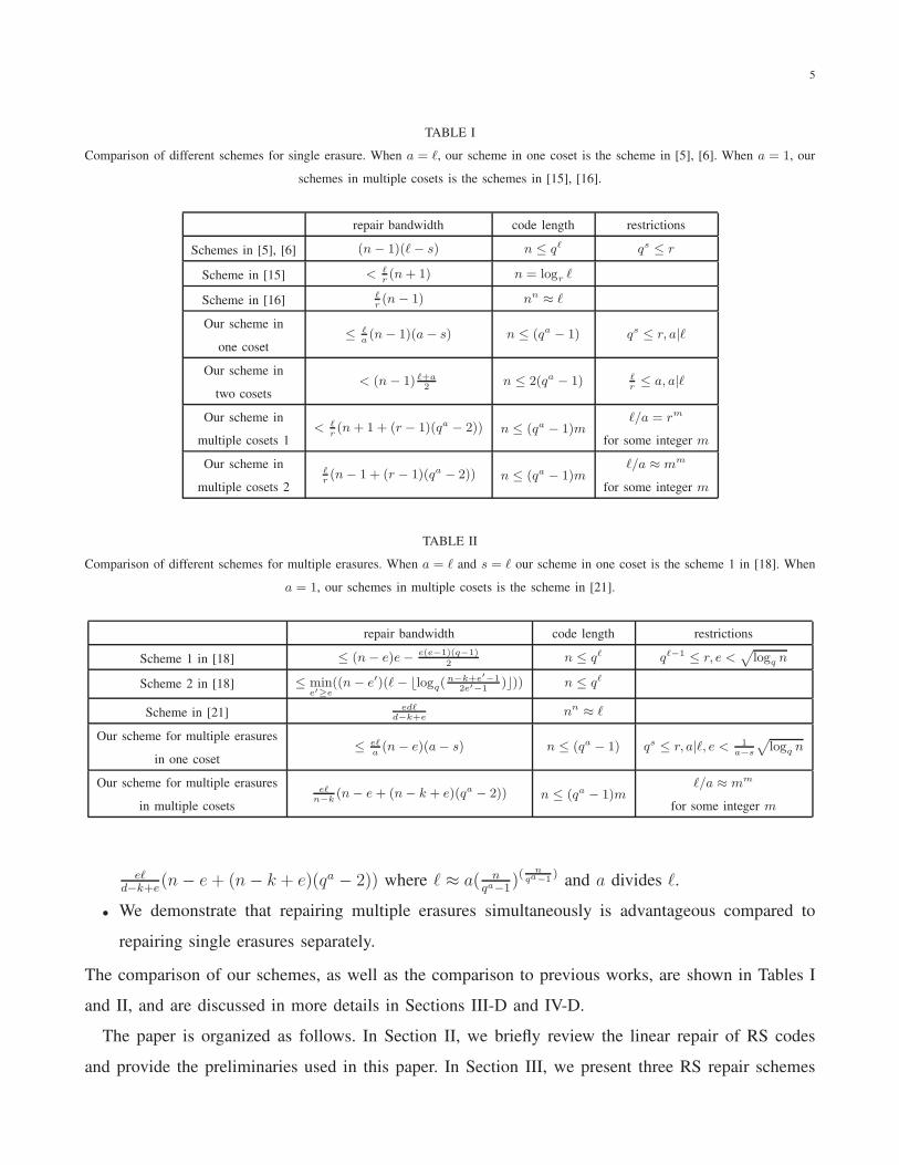
TABLE I

Comparison of different schemes for single erasure. When a = ℓ, our scheme in one coset is the scheme in [5], [6]. When a = 1, our

schemes in multiple cosets is the schemes in [15], [16].

repair bandwidth code length restrictions

Schemes in [5], [6] (n− 1)(ℓ− s) n ≤ qℓ qs ≤ r

Scheme in [15] < ℓr(n+ 1) n = logr ℓ

Scheme in [16]ℓr(n− 1) nn ≈ ℓ

Our scheme in

one coset≤ ℓ

a(n− 1)(a− s) n ≤ (qa − 1) qs ≤ r, a|ℓ

Our scheme in

two cosets< (n− 1) ℓ+a

2n ≤ 2(qa − 1) ℓ

r≤ a, a|ℓ

Our scheme in

multiple cosets 1< ℓ

r(n+ 1 + (r − 1)(qa − 2)) n ≤ (qa − 1)m

ℓ/a = rm

for some integer m

Our scheme in

multiple cosets 2

ℓr(n− 1 + (r − 1)(qa − 2)) n ≤ (qa − 1)m

ℓ/a ≈ mm

for some integer m

TABLE II

Comparison of different schemes for multiple erasures. When a = ℓ and s = ℓ our scheme in one coset is the scheme 1 in [18]. When

a = 1, our schemes in multiple cosets is the scheme in [21].

repair bandwidth code length restrictions

Scheme 1 in [18] ≤ (n− e)e− e(e−1)(q−1)2

n ≤ qℓ qℓ−1 ≤ r, e <√

logq n

Scheme 2 in [18] ≤ mine′≥e

((n− e′)(ℓ− ⌊logq(n−k+e′−1

2e′−1)⌋)) n ≤ qℓ

Scheme in [21]edℓ

d−k+enn ≈ ℓ

Our scheme for multiple erasures

in one coset≤ eℓ

a(n− e)(a− s) n ≤ (qa − 1) qs ≤ r, a|ℓ, e < 1

a−s

√

logq n

Our scheme for multiple erasures

in multiple cosets

eℓn−k

(n− e+ (n− k + e)(qa − 2)) n ≤ (qa − 1)mℓ/a ≈ mm

for some integer m

eℓd−k+e

(n− e+ (n− k + e)(qa − 2)) where ℓ ≈ a( nqa−1

)(n

qa−1) and a divides ℓ.

• We demonstrate that repairing multiple erasures simultaneously is advantageous compared to

repairing single erasures separately.

The comparison of our schemes, as well as the comparison to previous works, are shown in Tables I

and II, and are discussed in more details in Sections III-D and IV-D.

The paper is organized as follows. In Section II, we briefly review the linear repair of RS codes

and provide the preliminaries used in this paper. In Section III, we present three RS repair schemes

6

for single erasure. Then, we discuss the repair schemes for multiple erasures in Section IV. In Section

V, we provide the conclusion.

Notation: Throughout this paper, for positive integer i, we use [i] to denote the set {1, 2, . . . , i}.

For integers a, b, we use a | b to denote that a divides b. For real numbers an, bn, which are functions

of n, we use a ≈ b to denote limn→∞anbn

= 1. For sets A ⊆ B, we use B/A to denote the difference

of A from B. For a finite field F, we denote by F∗ = F/{0} the corresponding multiplicative group.

We write E ≤ F for E being a subfield of F. For element β ∈ F and E as a subset of F, we denote

βE = {βs, ∀s ∈ E}. AT denotes the transpose of the matrix A.

II. PRELIMINARIES

In this section, we review the linear repair scheme of RS code in [5], and provide a basic lemma

used in our proposed schemes.

The Reed-Solomon code RS(A, k) over F = GF (qℓ) of dimension k with n evaluation points

A = {α1, α2, . . . , αn} ⊆ F is defined as

RS(A, k) = {(f(α1), f(α2), . . . , f(αn)) : f ∈ F[x], deg(f) ≤ k − 1},

where deg() denotes the degree of a polynomial, f(x) = u0 + u1x + u2x2 + · · · + uk−1x

k−1, and

ui ∈ F, i = 0, 1, . . . , k − 1 are the messages. Every evaluation symbol f(α), α ∈ A, is called a code

word symbol or a storage node. The sub-packetization size is defined as ℓ, and r , n− k denotes the

number of parity symbols.

Assume e nodes fail, e ≤ n − k, and we want to recover them. The number of helper nodes are

denoted by d. The amount of information transmitted from the helper nodes is defined as the repair

bandwidth b, measured in the number of symbols over GF (q). All the remaining n− e = d nodes are

assumed to be the helper nodes unless stated otherwise. We define the normalized repair bandwidth

as bℓd

, which is the average fraction of information transmitted from each helper. By [7], [33], the

minimum storage regenerating (MSR) bound for the bandwidth is

b ≥eℓd

d− k + e. (2)

As mentioned before, codes achieving the MSR bound require large sub-packetization sizes. In this

section, we focus on the single erasure case.

Assume B ≤ F, namely, B is a subfield of F. A linear repair scheme requires some symbols of the

subfield B to be transmitted from each helper node [5]. If the symbols from the same helper node

7

are linearly dependent, the repair bandwidth decreases. In particular, the scheme uses dual code to

compute the failed node and uses trace function to obtain the transmitted subfield symbols, as detailed

below.

Assume f(α∗) fails for some α∗ ∈ A. For any polynomial p(x) ∈ F[x] of which the degree is

smaller than r, (υ1p(α1), υ2p(α2), . . . , υnp(αn)) is a dual codeword of RS(A, k), where υi, i ∈ [n]

are non-zero constants determined by the set A (see for example [1, Thm. 4 in Ch.10]). We can thus

repair the failed node f(α∗) from

υα∗p(α∗)f(α∗) = −n

∑

i=1,αi 6=α∗

υip(αi)f(αi) (3)

The summation on the right side means that we add all the i elements from i = 1 to i = n except

when αi 6= α∗.

The trace function from F onto B is defined as

trF/B(β) = β + βq + · · ·+ βqℓ−1

, (4)

where β ∈ F, B = GF (q) is called the base field, and q is a power of a prime number. It is a linear

mapping from F to B and satisfies

trF/B(αβ) = αtrF/B(β) (5)

for all α ∈ B.

We define the rank rankB({γ1, γ2, ..., γi}) to be the cardinality of a maximal subset of {γ1, γ2, ..., γi}

that is linearly independent over B. For example, for B = GF (2) and α /∈ B, rankB({1, α, 1+α}) = 2

because the subset {1, α} is the maximal subset that is linearly independent over B and the cardinality

of the subset is 2.

Assume we use polynomials pj(x), j ∈ [ℓ] to generate ℓ different dual codewords, called repair

polynomials. Combining the trace function and the dual code, we have

trF/B(υα∗pj(α∗)f(α∗)) = −

n∑

i=1,αi 6=α∗

trF/B(υipj(αi)f(αi)). (6)

In a repair scheme, the helper f(αi) transmits

{trF/B(υipj(αi)f(αi)) : j ∈ [ℓ]}. (7)

Suppose {υα∗p1(α∗), υα∗p2(α

∗), . . . , υα∗pℓ(α∗)} is a basis for F over B, and assume {µ1, µ2, . . . , µℓ}

is its dual basis. Then, f(α∗) can be repaired by

f(α∗) =

ℓ∑

j=1

µjtrF/B(υα∗pj(α∗)f(α∗)). (8)

8

Since υα∗ is a non-zero constant, we equivalently suppose that {p1(α∗), . . . , pℓ(α

∗)} is a basis.

In fact, by [5] any linear repair scheme of RS code for the failed node f(α∗) is equivalent to

choosing pj(x), j ∈ [ℓ], with degree smaller than r, such that {p1(α∗), . . . , pℓ(α

∗)} forms a basis for

F over B. We call this the full rank condition:

rankB({p1(α∗), p2(α

∗), . . . , pℓ(α∗)}) = ℓ. (9)

The repair bandwidth can be calculated from (7) and by noting that vif(αi) is a constant:

b =∑

α∈A,α6=α∗

rankB({p1(α), p2(α), . . . , pℓ(α)}). (10)

We call this the repair bandwidth condition.

The goal of a good RS code construction and its repair scheme is to choose appropriate evaluation

points A and polynomials pj(x), j ∈ [ℓ], that can reduce the repair bandwidth in (10) while satisfying

(9).

The following lemma is due to the structure of the multiplicative group of F, which will be used for

finding the evaluation points in the code constructions in this paper. Similar statements can be found

in [2, Ch. 2.6].

Lemma 1. Assume E ≤ F = GF (qℓ), then F∗ can be partitioned to t ,

qℓ−1|E|−1

cosets: {E∗, βE∗,

β2E∗, . . . , βt−1

E∗}, where β is a primitive element of F.

Proof: The qℓ − 1 elements in F∗ are {1, β, β2, . . . , βqℓ−2} and E

∗ ⊆ F∗. Assume that t is the

smallest nonzero number that satisfies βt ∈ E∗, then we know that βk ∈ E

∗ if and only if t|k.

Also, βk1 6= βk2 when k1 6= k2 and k1, k2 < qℓ − 2. Since there are only |E| − 1 nonzero distinct

elements in E∗ and βqℓ−1 = 1, we have t = qℓ−1

|E|−1and the t cosets are E

∗ = {1, βt, β2t, . . . , β(|E|−2)t},

βE∗ = {β, βt+1, β2t+1, . . . , β(|E|−2)t+1}, . . . , βt−1E∗ = {βt−1, β2t−1, β3t+1, . . . , β(|E|−1)t−1}.

III. REED-SOLOMON REPAIR SCHEMES FOR SINGLE ERASURE

In this section, we present our schemes in which the evaluation points are part of one coset, two

cosets and multiple cosets for a single erasure. From these constructions, we achieve several different

points on the tradeoff between the sub-packetization size and the normalized repair bandwidth. The

main ideas of the constructions are:

(i) In all our schemes, we take an original RS code, and construct a new code over a larger finite

field. Thus, the sub-packetization size ℓ is increased.

9

(ii) For the schemes using one and two cosets, the code parameters n, k are kept the same as the

original code. Hence, for given n, r = n− k, the sub-packetization size ℓ increases, but we show that

the normalized repair bandwidth remains the same.

(iii) For the scheme using multiple cosets, the code length n is increased and the redundancy r is

fixed. Moreover, the code length n grows faster than the sub-packetization size ℓ. Therefore, for fixed

n, r, the sub-packetization ℓ decreases, and we show that the normalized repair bandwidth is only

slightly larger than the original code.

A. Schemes in one coset

Assume E = GF (qa) is a subfield of F = GF (qℓ) and B = GF (q) is the base field, where q is

a prime number. The evaluation points of the code over F that we construct are part of one coset in

Lemma 1.

We first present the following lemma about the basis.

Lemma 2. Assume {ξ1, ξ2, . . . , ξℓ} is a basis for F = GF (qℓ) over B = GF (q), then {ξqs

1 , ξqs

2 , . . . , ξqs

ℓ },

s ∈ [ℓ] is also a basis.

Proof: Assume {ξqs

1 , ξqs

2 , . . . , ξqs

ℓ }, s ∈ [ℓ] is not a basis for F over B, then there exist nonzero

(α1, α2, . . . , αℓ), αi ∈ B, i ∈ [ℓ], that satisfy

α1ξqs

1 + α2ξqs

2 + · · ·+ αℓξqs

ℓ

=0

=(α1ξ1 + α2ξ2 + · · ·+ αℓξℓ)qs, (11)

which is in contradiction to the assumption that {ξ1, ξ2, . . . , ξℓ} is a basis for F over B.

The following theorem shows the repair scheme using one coset for the evaluation points.

Theorem 1. There exists an RS(n, k) code over F = GF (qℓ) with repair bandwidth b ≤ ℓa(n−1)(a−s)

symbols over B = GF (q), where q is a prime number and a, s satisfy n < qa, qs ≤ n− k, a|ℓ.

Proof: Assume a field F = GF (qℓ) is extended from E = GF (qa), a | ℓ, and β is a primitive

element of F. We focus on the code RS(A, k) of dimension k over F with evaluation points A =

{α1, α2, . . . , αn} ⊆ βmE∗ for some 0 ≤ m < qℓ−1

qa−1, which is one of the cosets in Lemma 1. The base

field is B = GF (q) and (6) is used to repair the failed node f(α∗).

10

Construction I: Inspired by [5], for s = a− 1, we choose

pj(x) =trE/B(ξj(

xβm − α∗

βm ))xβm − α∗

βm

, j ∈ [a], (12)

where {ξ1, ξ2, . . . , ξa} is a basis for E over B. The degree of pj(x) is smaller than r since qs ≤ r.

When x = α∗, by (4) we have

pj(α∗) = ξj. (13)

So, the polynomials satisfy

rankB({p1(α∗), p2(α

∗), . . . , pa(α∗)}) = a. (14)

When x 6= α∗, since trE/B(ξj(xβm − α∗

βm )) ∈ B, and xβm − α∗

βm is a constant independent of j, we have

rankB({p1(x), p2(x), . . . , pa(x)}) = 1. (15)

Let {η1, η2, η3, . . . , ηℓ/a} be a basis for F over E, the ℓ repair polynomials are chosen as

{η1pj(x), η2pj(x), . . . , ηℓ/apj(x) : j ∈ [a]}. (16)

Since pj(x) ∈ E, we can conclude that

rankB({η1pj(α∗), η2pj(α

∗), . . . , ηℓ/apj(α∗) : j ∈ [a]})

=ℓ

arankB({p1(α

∗), p2(α∗), . . . , pa(α

∗)}) = ℓ (17)

satisfies the full rank condition, and for x 6= α∗

rankB({η1pj(x), η2pj(x), . . . , ηℓ/apj(x) : j ∈ [a]})

=ℓ

arankB({p1(x), p2(x), . . . , pa(x)}) =

ℓ

a. (18)

From (10) we can calculate the repair bandwidth

b =ℓ

a(n− 1). (19)

Construction II: For s ≤ a− 1, inspired by [6], we choose

pj(x) = ξj

qs−1∏

i=1

(

x

βm−

(

α∗

βm− w−1

i ξj

))

, j ∈ [a], (20)

11

where {ξ1, ξ2, . . . , ξa} is a basis for E over B, and W = {w0 = 0, w1, w2, . . . , wqs−1} is an s-

dimensional subspace in E, s < a, qs ≤ r. It is easy to check that the degree of pj(x) is smaller

than r since qs ≤ r. When x = α∗, we have

pj(α∗) = ξq

s

j

qs−1∏

i=1

w−1i . (21)

Sinceqs−1∏

i=1

w−1i is a constant, from Lemma 2 we have

rankB({p1(α∗), p2(α

∗), . . . , pa(α∗)}) = a. (22)

For x 6= α∗, set x′ = α∗

βm − xβm ∈ E, we have

pj(x) = ξj

qs−1∏

i=1

(

x

βm−

(

α∗

βm− w−1

i ξj

))

= ξj

qs−1∏

i=1

(w−1i ξj − x′)

= ξj

qs−1∏

i=1

(w−1i x′)

qs−1∏

i=1

(ξj/x′ − wi)

= (x′)qs

qs−1∏

i=1

(w−1i )

qs−1∏

i=0

(ξj/x′ − wi). (23)

By [34, p. 4], g(y) =qs−1∏

i=0

(y −wi) is a linear mapping from E to itself with dimension a− s over B.

Since (x′)qsqs−1∏

i=1

(w−1i ) is a constant independent of j, we have

rankB({p1(x), p2(x), . . . , pa(x)}) ≤ a− s. (24)

Let {η1, η2, η3, . . . , ηℓ/a} be a basis for F over E, then the ℓ polynomials are chosen as {η1pj(x),

η2pj(x), . . . , ηℓ/apj(x), j ∈ [a]}. From (21) and (23) we know that pj(x) ∈ E, so we can conclude that

rankB({η1pj(α∗), η2pj(α

∗), . . . , ηℓ/apj(α∗) : j ∈ [a]})

=ℓ

arankB({p1(α

∗), p2(α∗), . . . , pa(α

∗)}) = ℓ (25)

satisfies (9), and for x 6= α∗

rankB({η1pj(x), η2pj(x), . . . , ηℓ/apj(x) : j ∈ [a]})

=ℓ

arankB({p1(x), p2(x), . . . , pa(x)}) ≤

ℓ

a(a− s). (26)

12

Now from (10) we can calculate the repair bandwidth

b ≤ℓ

a(n− 1)(a− s). (27)

Combining (19) and (27) will complete the proof of Theorem 1.

Rather than directly using the schemes in [5] and [6], the polynomials (12) and (20) that we use

are similar to [5] and [6], respectively, but are mappings from E to B. Moreover, we multiply each

polynomial with the basis for F over E to satisfy the full rank condition. In this case, our scheme

significantly reduces the repair bandwidth when the code length remains the same. Our evaluation

points are in a coset rather than the entire field F as in [5] and [6]. It should be noted that a here can

be an arbitrary number that divides ℓ and when a = ℓ, our schemes are exactly the same as those in

[5] and [6]. Note that the normalized repair bandwidth bℓ(n−1)

decreases as a decreases. Therefore, our

scheme outperforms those in [5] and [6] when applied to the case of ℓ > logq n.

Example 1. Assume q = 2, ℓ = 9, a = 3 and E = {0, 1, α, α2, . . . , α6}. Let A = E∗, n = 7, k = 5 so

r = n − k = 2. Choose s = log2 r = 1 and W = {0, 1} in Construction II. Then, we have pj(x) =

ξj(x−α∗+ξj). Let {ξ1, ξ2, ξ3} be {1, α, α2}. It is easy to check that rankB({p1(α∗), p2(α

∗), p3(α∗)}) =

3 and rankB({p1(x), p2(x), p3(x)}) = 2 for x 6= α∗. Therefore the repair bandwidth is b = 36 bits as

suggested in Theorem 1. For the same (n, k, ℓ), the repair bandwidth in [6] is 48 bits. For another

example, consider RS(14, 10) code used in Facebook [32], we have repair bandwidth of 52 bits for

ℓ = 8, while [6] requires 60 bits and the naive scheme requires 80 bits.

Remark 1. The schemes in [5] and [6] can also be used in an RS code over E with repair bandwidth

(n − 1)(a − s), and with ℓ/a copies of the code. Thus, they can also reach the repair bandwidth of

ℓa(n− 1)(a− s). It should be noted that by doing so, the code is a vector code, however our scheme

constructs a scalar code. To the best of our knowledge, this is the first example of such a scalar code

in the literature.

B. Schemes in two cosets

Now we discuss our scheme when the evaluation points are chosen from two cosets. In this scheme,

we choose the polynomials that have full rank when evaluated at the coset containing the failed node,

and rank 1 when evaluated at the other coset.

Theorem 2. There exists an RS(n, k) code over F = GF (qℓ) with repair bandwidth b < (n− 1) ℓ+a2

symbols over B = GF (q), where q is a prime number and a satisfies n ≤ 2(qa − 1), a|ℓ, ℓa≤ n− k.

13

Proof: Assume a field F = GF (qℓ) is extended from E = GF (qa) and β is the primitive element

of F. We focus on the code RS(A, k) over F of dimension k with evaluation points A consisting

of n/2 points from βm1E∗ and n/2 points from βm2E

∗, 0 ≤ m1 < m2 ≤ qℓ−1qa−1

and m2 −m1 = qs,

s ∈ {0, 1, . . . , ℓa}.

In this case we view E as the base field and repair the failed node f(α∗) by

trF/E(υα∗pj(α∗)f(α∗)) = −

n∑

i=1,αi 6=α∗

trF/E(υipj(αi)f(αi)). (28)

Inspired by [5, Theorem 10], for j ∈ [ ℓa], we choose

pj(x) =

( xβm2

)j−1, if α∗ ∈ βm1E∗,

( xβm1

)j−1, if α∗ ∈ βm2E∗.

(29)

The degree of pj(x) is smaller than r when ℓa≤ r. Then, we check the rank in each case.

When α∗ ∈ βm2E∗, if x = βm1γ ∈ βm1E

∗, for some γ ∈ E∗,

pj(x) =

(

x

βm1

)j−1

= γj−1, (30)

so

rankE({p1(x), p2(x), . . . , p ℓa(x)}) = 1. (31)

If x = βm2γ ∈ βm2E∗, for some γ ∈ E

∗,

pj(x) =

(

x

βm1

)j−1

= (βm2−m1)j−1γj−1. (32)

Since m2 −m1 = qs and {1, β, β2, . . . , βℓa−1} is the polynomial basis for F over E, from Lemma 2

we know that

rankE({p1(x), p2(x), . . . , p ℓa(x)}) =

ℓ

a. (33)

When α∗ ∈ βm1E∗, if x = βm1γ ∈ βm1E

∗, for some γ ∈ E∗,

pj(x) =

(

x

βm2

)j−1

= (βm1−m2)j−1γj−1

= (βm2−m1)1−ℓa (βm2−m1)

ℓa−jγj−1. (34)

Since (βm2−m1)1−ℓa is a constant, from Lemma 2 we know that

rankE({p1(x), p2(x), . . . , p ℓa(x)}) =

ℓ

a. (35)

14

If x = βm2γ ∈ βm2E∗, for some γ ∈ E

∗,

pj(x) =

(

x

βm2

)j−1

= γj−1, (36)

so

rankE({p1(x), p2(x), . . . , p ℓa(x)}) = 1. (37)

Therefore, {pj(α∗), j ∈ [ ℓ

a]} has full rank over E, for any evaluation point α∗ ∈ A. For x from the

coset containing α∗, the polynomials have rank ℓ/a, and for x from the other coset, the polynomials

have rank 1. Then, the repair bandwidth in symbols over B can be calculated from (10) as

b =ℓ

a(n

2− 1) logq |E|+

n

2logq |E|

= (n− 1)ℓ+ a

2−

ℓ− a

2

< (n− 1)ℓ+ a

2. (38)

Thus, the proof is completed.

Example 2. Take the RS(14, 11) code over F = GF (212) for example. Let β be the primitive element

in F, a = 4, s = ℓ/a = 3 and A = E∗ ∪ βE∗. Assume α∗ ∈ βE∗, then {pj(x), j ∈ [3]} is the set

{1, x, x2}. It is easy to check that when x ∈ βE∗ the polynomials have full rank and when x ∈ E∗

the polynomials have rank 1. The total repair bandwidth is 100 bits. For the same (n, k, ℓ), the repair

bandwidth of our scheme in one coset is 117 bits. For the scheme in [5], which only works for ℓ/a = 2,

we can only choose a = 6 and get the repair bandwidth of 114 bits for the same (n, k, ℓ).

C. Schemes in multiple cosets

In the schemes in this subsection, we extend an original code to a new code over a larger field and

the evaluation points are chosen from multiple cosets in Lemma 1 to increase the code length. The

construction ensures that for fixed n, the sub-packetization size is smaller than the original code. If

the original code satisfies several conditions to be discussed soon, the repair bandwidth in the new

code is only slightly larger than that of the original code. Particularly, if the original code is an MSR

code, then we can get the new code in a much smaller sub-packetization level with a small extra repair

bandwidth. Also, if the original code works for any number of helpers and multiple erasures, the new

code works for any number of helpers and multiple erasures, too. We discuss multiple erasures in

Section IV.

15

We first prove a lemma regarding the ranks over different base fields, and then describe the new

code.

Lemma 3. Let B = GF (q),F′ = GF (qℓ′

),E = GF (qa), F = GF (qℓ), ℓ = aℓ′. a and ℓ′ are relatively

prime and q can be any power of a prime number. For any set of {γ1, γ2, ..., γℓ′} ⊆ F′ ≤ F, we have

rankE({γ1, γ2, ..., γℓ′})

=rankB({γ1, γ2, ..., γℓ′}). (39)

Proof: Assume rankB({γ1, γ2, ..., γℓ′}) = c and without loss of generality, {γ1, γ2, ..., γc} are lin-

early independent over B. Then, we can construct {γ′c+1, γ

′c+2, ..., γ

′ℓ′} ⊆ F

′ to make {γ1, γ2, ..., γc, γ′c+1,

γ′c+2, ..., γ

′ℓ′} form a basis for F′ over B.

Assume we get F by adjoining β to B. Then, from [35, Theorem 1.86] we know that {1, β, β2, ..., βℓ′−1}

is a basis for both F over E, and F′ over B. So, any symbol y ∈ F can be presented as a linear combina-

tion of {1, β, β2, ..., βℓ′−1} with some coefficients in E. Also, we know that there is an invertible linear

transformation with coefficients in B between {γ1, γ2, ..., γc, γ′c+1, γ

′c+2, ..., γ

′ℓ′} and {1, β, β2, ..., βℓ′−1},

because they are a basis for F′ over B. Combined with the fact that {1, β, β2, ..., βℓ′−1} is also a basis

for F over E, we can conclude that any symbol y ∈ F can be represented as

y = x1γ1 + x2γ2 + ...+ xcγc + xc+1γ′c+1 + ...+ xℓγ

′ℓ′ (40)

with some coefficients xi ∈ E, which means that {γ1, γ2, ..., γc, γ′c+1, γ

′c+2, ..., γ

′ℓ′} is also a basis for

F over E. Then, we have that {γ1, γ2, ..., γc} are linearly independent over E,

rankE({γ1, γ2, ..., γℓ′})

≥c

=rankB({γ1, γ2, ..., γℓ′}). (41)

Since B ≤ E, we also have

rankE({γ1, γ2, ..., γℓ′})

≤rankB({γ1, γ2, ..., γℓ′}). (42)

The proof is completed.

Theorem 3. Assume there exists a RS(n′, k′) code E′ over F′ = GF (qℓ

′

) with evaluation points set

A′. The evaluation points are linearly independent over B = GF (q). The repair bandwidth is b′ and the

16

repair polynomials are p′j(x). Then, we can construct a new RS(n, k) code E over F = GF (qℓ), ℓ = aℓ′

with n = (qa − 1)n′, k = n − n′ + k′ and repair bandwidth of b = ab′(qa − 1) + (qa − 2)ℓ symbols

over B = GF (q) if we can find new repair polynomials pj(x) ∈ F[x], j ∈ [ℓ′], with degrees less than

n− k that satisfy

rankE({p1(x), p2(x), . . . , pℓ′(x)})

=rankB({p′1(α), p

′2(α), . . . , p

′ℓ′(α)}) (43)

for all α ∈ A′, x ∈ αE∗, where E = GF (qa).

Proof: We first prove the case when a and ℓ′ are necessarily relatively prime using Lemma 3,

the case when a and ℓ′ are not relatively prime are proved in Appendix A. Assume the evaluation

points of E′ are A′ = {α1, α2, . . . , αn′}, then from Lemma 3 we know that they are also linearly

independent over E, so there does not exist γi, γj ∈ E∗ that satisfy αiγi = αjγj , which implies that

{α1E∗, α2E

∗, . . . , αn′E∗} are distinct cosets. Then, we can extend the evaluation points to be

A = {α1E∗, α2E

∗, . . . , αn′E∗}. (44)

and n = (qa − 1)n′. We keep the same redundancy r = n′ − k′ for the new code so k = n− r.

For the new code E , we use pj(x) ∈ F[x], j ∈ [ℓ′] to repair the failed node f(α∗)

trF/E(υα∗pj(α∗)f(α∗)) = −

∑

α∈A,α6=α∗

trF/E(υαpj(α)f(α)). (45)

Assume the failed node is f(α∗) and α∗ ∈ αiE∗. Then, for the node x ∈ αiE

∗, because the original

code satisfies the full rank condition, we have

rankE({p1(x), p2(x), . . . , pℓ′(x)})

=rankB({p′1(αi), p

′2(αi), . . . , p

′ℓ′(αi)}) = ℓ′, (46)

then we can recover the failed node with pj(x), and each helper in the coset containing the failed

node transmits ℓ′ symbols over E.

For a helper in the other cosets, x ∈ αǫE∗, ǫ 6= i, by (43),

rankE({p1(x), p2(x), . . . , pℓ′(x)})

=rankB({p′1(αǫ), p

′2(αǫ), . . . , p

′ℓ′(αǫ)}), (47)

then every helper in these cosets transmits b′

n′−1symbols in E on average.

17

The repair bandwidth of the new code can be calculated from the repair bandwidth condition (10)

as

b =b′

n′ − 1· (n′ − 1)|E∗| · a+ (|E∗| − 1)ℓ′ · a

= ab′(qa − 1) + (qa − 2)ℓ (48)

which completes the proof.

Note that the calculation in (48) and (38) are similar in the sense that a helper in the coset containing

the failure naively transmits the entire stored information, and the other helpers use the bandwidth

that is the same as the original code.

As a special case of Theorem 3, when b′ = ℓ′

r(n′ − 1) matching the MSR bound (1), we get

b =ℓ

r(n− 1) +

ℓ

r(r − 1)(qa − 2), (49)

where the second term is the extra bandwidth compared to the MSR bound.

Next, we apply Theorem 3 to the near-MSR code [15] and the MSR code [16]. The first realization

of the scheme in multiple cosets is inspired by [15].

Theorem 4. There exists an RS(n, k) code over F = GF (qℓ) of which n = (qa − 1) logrℓa

and a|ℓ,

such that the repair bandwidth satisfies b < ℓn−k

[n + 1 + (n − k − 1)(qa − 2)], measured in symbols

over B = GF (q) for some prime number q.

Proof: We first prove the case when a and ℓ′ are relatively prime using Lemma 3, the case when

a and ℓ′ are not necessarily relatively prime are proved in Appendix A. We use the code in [15] as

the original code. The original code is defined in F′ = GF (qℓ

′

) and ℓ′ = rn′

. The evaluation points

are A′ = {β, βr, βr2, . . . , βrn′−1

} where β is a primitive element of F′.

In the original code, for c = 0, 1, 2, . . . , ℓ′ − 1, we write its r-ary expansion as c = (cn′cn′−1 . . . c1),

where 0 ≤ ci ≤ r− 1 is the i-th digit from the right. Assuming the failed node is f(βri−1), the repair

polynomials are chosen to be

p′j(x) = βcxs, ci = 0, s = 0, 1, 2, . . . , r − 1, x ∈ F′. (50)

Here c varies from 0 to ℓ′−1 given that ci = 0, and s varies from 0 to r−1. So, we have ℓ′ polynomials

in total. The subscript j is indexed by c and s, and by a small abuse of the notation, we write j ∈ [ℓ′].

In the new code, let us define E = GF (qa) of which a and ℓ′ are relatively prime. Adjoining β to

E, we get F = GF (qℓ), ℓ = aℓ′. The new evaluation points are A = {βE∗, βrE∗, βr2

E∗, . . . , βrn

′−1E∗}.

18

Since A′ is part of the polynomial basis for F′ over B, we know that {β, βr, βr2, . . . , βrn

′−1} are

linearly independent over B. Hence, we can apply Lemma 3 and the cosets are distinct, resulting in

n = |A| = (qa − 1) logrℓa.

In our new code, let us assume the failed node is f(α∗) and α∗ ∈ βri−1C, and we choose the

polynomial pj(x) with the same form as p′j(x),

pj(x) = βcxs, ci = 0, s = 0, 1, 2, . . . , r − 1, x ∈ F. (51)

For nodes corresponding to x = βrtγ ∈ βrtE∗, for some γ ∈ E

∗, we know that

pj(x) = βcxs = βc(γβrt)s = γsp′j(βrt). (52)

Since p′j(βrt) ∈ F

′, from Lemma 3, we have

rankE({γsp′1(β

rt), γsp′2(βrt), . . . , γsp′ℓ′(β

rt)})

=rankE({p′1(β

rt), p′2(βrt), . . . , p′ℓ′(β

rt)})

=rankB({p′1(β

rt), p′2(βrt), . . . , p′ℓ′(β

rt)}), (53)

which satisfies (43). Since the repair bandwidth of the original code is b′ < (n′ + 1) ℓ′

r, from (48) we

can calculate the repair bandwidth as

b = ab′(qa − 1) + (qa − 2)ℓ

<ℓ

r[n + 1 + (r − 1)(qa − 2)], (54)

where the second term is the extra bandwidth compared to the original code.

Example 3. We take an RS(4, 2) code in GF (216) as the original code and extend it with a =

3, |E∗| = 7 to an RS(28, 26) code in GF (248) with normalized repair bandwidth of b(n−1)ℓ

< 0.65. The

RS(28, 26) code in [15] achieves the normalized repair bandwidth of b(n−1)ℓ

< 0.54, while it requires

ℓ = 2.7 × 108. Our scheme has a much smaller ℓ compared to the scheme in [15] while the repair

bandwidth is a bit larger.

In the above theorem, we extend [15] to a linearly larger sub-packetization and an exponentially

larger code length, which means that for the same code length, we can have a much smaller sub-

packetization level.

Next, we show our second realization of the scheme in multiple cosets, which is inspired by [16].

Different from the previous constructions, this one allows any number of helpers, k ≤ d ≤ n− 1. The

19

sub-packetization size in the original code of [16] satisfies ℓ′ ≈ (n′)n′

when n′ grows to infinity, thus

in our new code it satisfies ℓ ≈ a(n′)n′

for some integer a.

Theorem 5. Let q be a prime number. There exists an RS(n, k) code over F = GF (qℓ) of which

ℓ = asq1q2...q nqa−1

, where qi is the i-th prime number that satisfies s|(qi − 1), s = d − k + 1 and

a is some integer. d is the number of helpers, k ≤ d ≤ (n − 1). The average repair bandwidth is

b = dℓ(n−1)(d−k+1)

[n− 1 + (d− k)(qa − 2)] measured in symbols over B = GF (q).

Proof: We first prove the case when a and ℓ′ are relatively prime using Lemma 3, the case when

a and ℓ′ are not necessarily relatively prime are proved in Appendix A. We use the code in [16]

as the original code, where the number of helpers is d′. We set n − k = n′ − k′ and calculate the

repair bandwidth for d helpers from the original code when d′ = d − k + k′. Let us define Fq(α)

to be the field obtained by adjoining α to the base field B. Similarly, we define Fq(α1, α2, . . . , αn)

for adjoining multiple elements. Let αi be an element of order qi over B. The code is defined in the

field F′ = GF (qℓ

′

) = GF (qsq1q2...,qn′ ), which is the degree-s extension of Fq(α1, α2, . . . , αn′). The

evaluation points are A′ = {α1, α2, . . . , αn′}.

Assuming the failed node is f(αi) and the helpers are chosen from the set R′, |R′| = d′, the

base field for repair is F′i, defined as F

′i , Fq(αj, j ∈ [n′], j 6= i). The repair polynomials are

{ηtp′j(αi), t ∈ [qi], j ∈ [s]}, where

p′j(x) = xj−1g′(x), j ∈ [s], x ∈ F′, (55)

g′(x) =∏

α∈A/(R′∪{αi})

(x− α), x ∈ F′. (56)

and ηt ∈ F′, t ∈ [qi], are constructed in [16] such that {ηtp

′j(αi), t ∈ [qi], j ∈ [s]} forms the basis for

F′ over F′

i. The repair is done using

trF′/F′i(υαi

ηtp′j(αi)f

′(αi)) = −n′∑

ǫ=1,ǫ 6=i

trF′/F′i(υǫηtp

′j(αǫ)f

′(αǫ)). (57)

For x /∈ R′ ∪ {αi}, p′j(x) = 0, so no information is transmitted. The original code reaches the MSR

repair bandwidth

b′ =∑

ǫ∈R′

rankF′i({ηtp

′j(αǫ) : t ∈ [qi], j ∈ [s]})

=d′ℓ′

d′ − k′ + 1. (58)

20

In our new code, we define E = GF (qa) = Fq(αn+1) where a and ℓ′ are relatively prime, and αn+1 is

an element of order a over B. Adjoining the primitive element of F′ to E, we get F = GF (qℓ), ℓ = aℓ′.

The new code is defined in F. We extend the evaluation points to be A = {α1E∗, α2E

∗, . . . , αn′E∗}.

Since {α1, α2, ..., αn′} are linearly independent over B, we can apply Lemma 3 and the cosets are

distinct. So, n = |A| = (qa − 1)n′.

Assuming the failed node is f(α∗) and α∗ ∈ αiE∗ and the helpers are chosen from the set R,

|R| = d, the base field for repair is Fi, which is defined by Fi , Fq(αj, j ∈ [n+1], j 6= i), for i ∈ [n].

We define the repair polynomials {ηtpj(x), t ∈ [qi], j ∈ [s]}, where

pj(x) = xj−1g(x), j ∈ [s], x ∈ F, (59)

g(x) =∏

α∈A/(R∪{α∗})

(x− α), x ∈ F, (60)

and ηt is the same as that in the original code. Then, we repair the failed node by

trF/Fi(υα∗ηtpj(α

∗)f(α∗)) = −∑

α∈A,α6=α∗

trF/Fi(υαηtpj(α)f(α)). (61)

For x ∈ αE∗, α ∈ A′, we have

pj(x) = γj−1αj−1g(x), j ∈ [s], (62)

for some γ ∈ E∗. If x /∈ R ∪ {α∗}, since g(x) = 0, no information is transmitted from node x. Next,

we consider all other nodes.

For x = αγ, α ∈ A′, since g(x) is a constant independent of j, γ ∈ E ⊆ Fi and ηt, αi ∈ F′, from

Lemma 3 we have

rankFi({ηtp1(x), ηtp2(x), . . . , ηtps(x) : t ∈ [qi]})

=rankFi({ηt, ηtγα, . . . , ηtγ

s−1αs−1 : t ∈ [qi]})

=rankFi({ηt, ηtα, . . . , ηtα

s−1 : t ∈ [qi]})

=rankF′i({ηt, ηtα, . . . , ηtα

s−1 : t ∈ [qi]})

=rankF′i({ηtp

′1(α), ηtp

′2(α), . . . , ηtp

′s(α) : t ∈ [qi]}), (63)

which satisfies (43).

21

When k ≤ d < n− 1, assuming the helpers are randomly chosen from all the remaining nodes, the

average repair bandwidth for different choices of the helpers can be calculated as

b = d

[

b′a

d′·n− 1− (qa − 2)

n− 1+ ℓ′a ·

qa − 2

n− 1

]

(64)

=dℓ

d− k + 1+

d

n− 1

ℓ

d− k + 1(d− k)(qa − 2). (65)

Here in (64) the second term corresponds to the helpers in the failed node coset, the first term

corresponds to the helpers in the other cosets, and in (65) we used d′ − k′ = d− k.

In the case of d = n− 1, the repair bandwidth of the code in Theorem 5 can be directly calculated

from (48) as

b = ab′(qa − 1) + (qa − 2)ℓ

=ℓ

r(n− 1) +

ℓ

r(r − 1)(qa − 2)]. (66)

In (65) and (66), the second term is the extra repair bandwidth compared to the original code.

In Theorems 4 and 5, we constructed our schemes by extending previous schemes. However, it should

be noted that since we only used the properties of the polynomials p′j(x), we have no restrictions on

the dimensions k′ of the original codes. So, in some special cases, even if k′ is negative and the

original codes do not exist, our theorems still hold. Thus, we can provide more feasible points of

(n, k) using our schemes. This is illustrated in the example below.

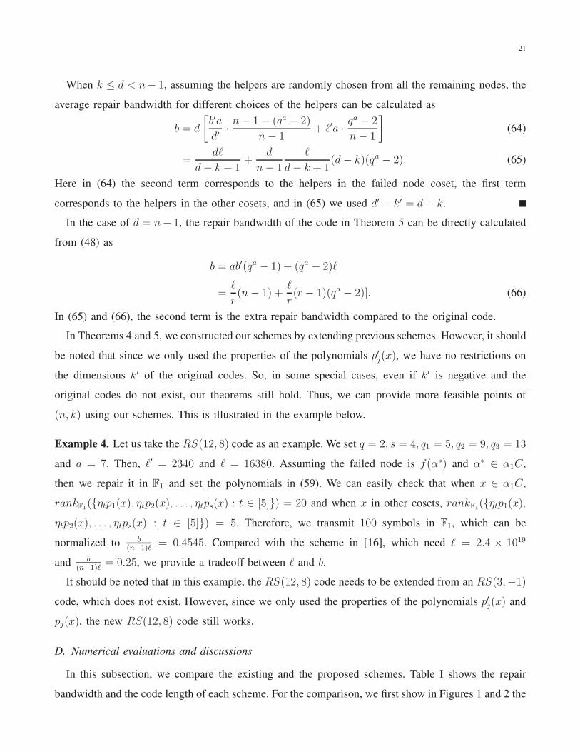
Example 4. Let us take the RS(12, 8) code as an example. We set q = 2, s = 4, q1 = 5, q2 = 9, q3 = 13

and a = 7. Then, ℓ′ = 2340 and ℓ = 16380. Assuming the failed node is f(α∗) and α∗ ∈ α1C,

then we repair it in F1 and set the polynomials in (59). We can easily check that when x ∈ α1C,

rankF1({ηtp1(x), ηtp2(x), . . . , ηtps(x) : t ∈ [5]}) = 20 and when x in other cosets, rankF1({ηtp1(x),

ηtp2(x), . . . , ηtps(x) : t ∈ [5]}) = 5. Therefore, we transmit 100 symbols in F1, which can be

normalized to b(n−1)ℓ

= 0.4545. Compared with the scheme in [16], which need ℓ = 2.4 × 1019

and b(n−1)ℓ

= 0.25, we provide a tradeoff between ℓ and b.

It should be noted that in this example, the RS(12, 8) code needs to be extended from an RS(3,−1)

code, which does not exist. However, since we only used the properties of the polynomials p′j(x) and

pj(x), the new RS(12, 8) code still works.

D. Numerical evaluations and discussions

In this subsection, we compare the existing and the proposed schemes. Table I shows the repair

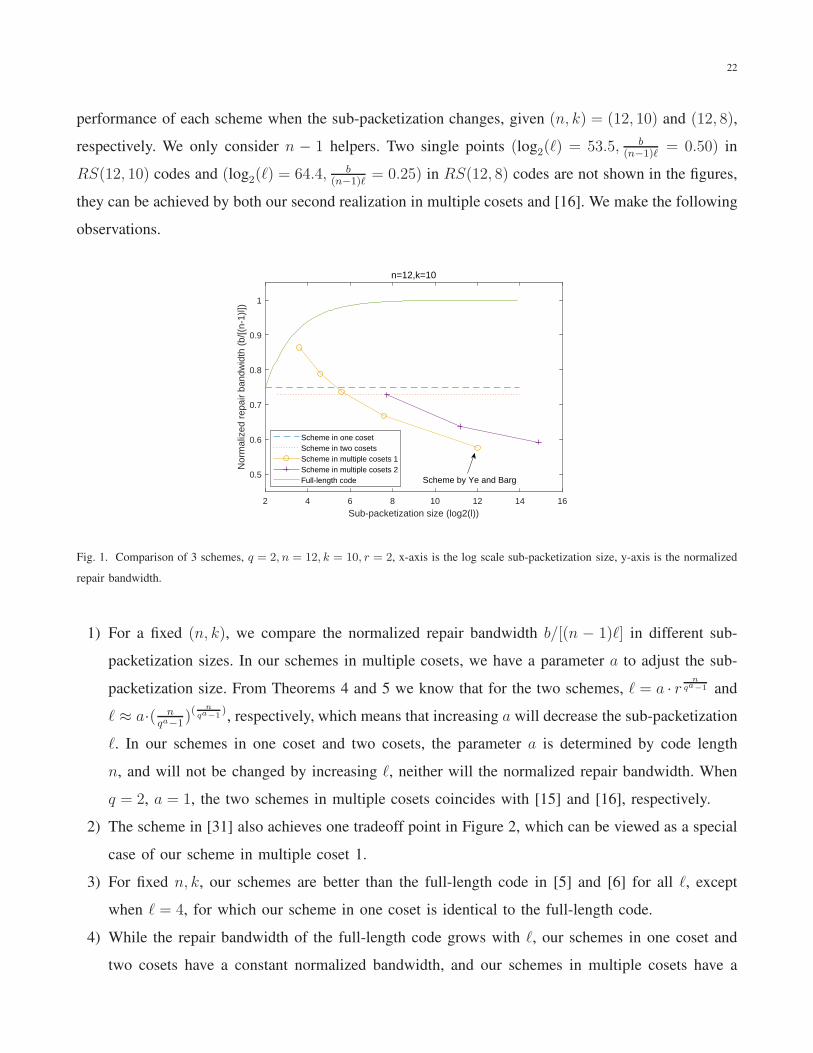
bandwidth and the code length of each scheme. For the comparison, we first show in Figures 1 and 2 the

22

performance of each scheme when the sub-packetization changes, given (n, k) = (12, 10) and (12, 8),

respectively. We only consider n − 1 helpers. Two single points (log2(ℓ) = 53.5, b(n−1)ℓ

= 0.50) in

RS(12, 10) codes and (log2(ℓ) = 64.4, b(n−1)ℓ

= 0.25) in RS(12, 8) codes are not shown in the figures,

they can be achieved by both our second realization in multiple cosets and [16]. We make the following

observations.

2 4 6 8 10 12 14 16

Sub-packetization size (log2(l))

0.5

0.6

0.7

0.8

0.9

1

Nor

mal

ized

rep

air

band

wid

th (

b/[(

n-1)

l])

n=12,k=10

Scheme in one cosetScheme in two cosetsScheme in multiple cosets 1Scheme in multiple cosets 2Full-length code Scheme by Ye and Barg

Fig. 1. Comparison of 3 schemes, q = 2, n = 12, k = 10, r = 2, x-axis is the log scale sub-packetization size, y-axis is the normalized

repair bandwidth.

1) For a fixed (n, k), we compare the normalized repair bandwidth b/[(n − 1)ℓ] in different sub-

packetization sizes. In our schemes in multiple cosets, we have a parameter a to adjust the sub-

packetization size. From Theorems 4 and 5 we know that for the two schemes, ℓ = a · rn

qa−1 and

ℓ ≈ a·( nqa−1

)(n

qa−1), respectively, which means that increasing a will decrease the sub-packetization

ℓ. In our schemes in one coset and two cosets, the parameter a is determined by code length

n, and will not be changed by increasing ℓ, neither will the normalized repair bandwidth. When

q = 2, a = 1, the two schemes in multiple cosets coincides with [15] and [16], respectively.

2) The scheme in [31] also achieves one tradeoff point in Figure 2, which can be viewed as a special

case of our scheme in multiple coset 1.

3) For fixed n, k, our schemes are better than the full-length code in [5] and [6] for all ℓ, except

when ℓ = 4, for which our scheme in one coset is identical to the full-length code.

4) While the repair bandwidth of the full-length code grows with ℓ, our schemes in one coset and

two cosets have a constant normalized bandwidth, and our schemes in multiple cosets have a

23

0 5 10 15 20 25

Sub-packetization size (log2(l))

0.2

0.3

0.4

0.5

0.6

0.7

0.8

0.9

1

Nor

mal

ized

rep

air

band

wid

th (

b/[(

n-1)

l])

n=12,k=8

Scheme in one cosetScheme in two cosetsScheme in multiple cosets 1Scheme in multiple cosets 2Full-length code

Scheme by Ye and Barg

Scheme by Chowdhury and Vardy

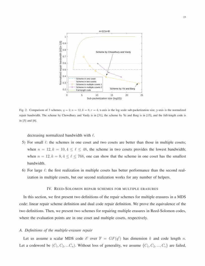
Fig. 2. Comparison of 3 schemes, q = 2, n = 12, k = 8, r = 4, x-axis is the log scale sub-packetization size, y-axis is the normalized

repair bandwidth. The scheme by Chowdhury and Vardy is in [31], the scheme by Ye and Barg is in [15], and the full-length code is

in [5] and [6].

decreasing normalized bandwidth with ℓ.

5) For small ℓ: the schemes in one coset and two cosets are better than those in multiple cosets;

when n = 12, k = 10, 4 ≤ ℓ ≤ 48, the scheme in two cosets provides the lowest bandwidth;

when n = 12, k = 8, 4 ≤ ℓ ≤ 768, one can show that the scheme in one coset has the smallest

bandwidth.

6) For large ℓ: the first realization in multiple cosets has better performance than the second real-

ization in multiple cosets, but our second realization works for any number of helpers.

IV. REED-SOLOMON REPAIR SCHEMES FOR MULTIPLE ERASURES

In this section, we first present two definitions of the repair schemes for multiple erasures in a MDS

code: linear repair scheme definition and dual code repair definition. We prove the equivalence of the

two definitions. Then, we present two schemes for repairing multiple erasures in Reed-Solomon codes,

where the evaluation points are in one coset and multiple cosets, respectively.

A. Definitions of the multiple-erasure repair

Let us assume a scalar MDS code E over F = GF (qℓ) has dimension k and code length n.

Let a codeword be (C1, C2, ...Cn). Without loss of generality, we assume {C1, C2, ..., Ce} are failed,

24

e ≤ n − k, and we repair them in the base field B = GF (q), where q can be any power of a prime

number. We also assume that we use all the remaining d = n − e nodes as helpers. The following

definitions are inspired by [5] for single erasure.

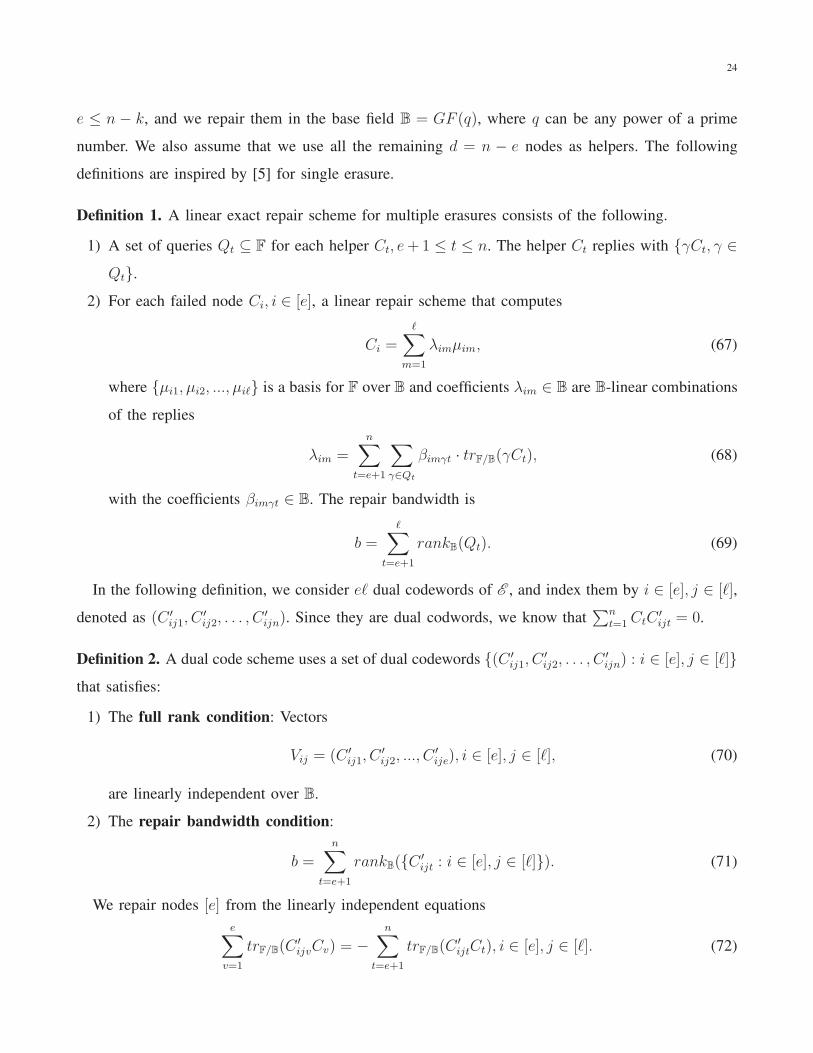
Definition 1. A linear exact repair scheme for multiple erasures consists of the following.

1) A set of queries Qt ⊆ F for each helper Ct, e+1 ≤ t ≤ n. The helper Ct replies with {γCt, γ ∈

Qt}.

2) For each failed node Ci, i ∈ [e], a linear repair scheme that computes

Ci =

ℓ∑

m=1

λimµim, (67)

where {µi1, µi2, ..., µiℓ} is a basis for F over B and coefficients λim ∈ B are B-linear combinations

of the replies

λim =n

∑

t=e+1

∑

γ∈Qt

βimγt · trF/B(γCt), (68)

with the coefficients βimγt ∈ B. The repair bandwidth is

b =ℓ

∑

t=e+1

rankB(Qt). (69)

In the following definition, we consider eℓ dual codewords of E , and index them by i ∈ [e], j ∈ [ℓ],

denoted as (C ′ij1, C

′ij2, . . . , C

′ijn). Since they are dual codwords, we know that

∑nt=1CtC

′ijt = 0.

Definition 2. A dual code scheme uses a set of dual codewords {(C ′ij1, C

′ij2, . . . , C

′ijn) : i ∈ [e], j ∈ [ℓ]}

that satisfies:

1) The full rank condition: Vectors

Vij = (C ′ij1, C

′ij2, ..., C

′ije), i ∈ [e], j ∈ [ℓ], (70)

are linearly independent over B.

2) The repair bandwidth condition:

b =

n∑

t=e+1

rankB({C′ijt : i ∈ [e], j ∈ [ℓ]}). (71)

We repair nodes [e] from the linearly independent equations

e∑

v=1

trF/B(C′ijvCv) = −

n∑

t=e+1

trF/B(C′ijtCt), i ∈ [e], j ∈ [ℓ]. (72)

25

Here we use the same condition names as the single erasure case, but in this section, they are

defined for multiple erasures.

Theorem 6. Definitions 1 and 2 are equivalent.

The equivalence of Definitions 1 and 2 follows similarly as arguments in [5], except that we need

to first solve e failed nodes simultaneously and then find out the form of each individual failure (67).

The detailed proof of Theorem 6 is shown in Appendix B, part of which uses Lemma 4 in Section

IV-B.

Remark 2. In this paper, we focus on repairing RS code and apply Theorem 6 to RS code. From [1,

Thm. 4 in Ch. 10] we know that with the polynomial pij(x) ∈ F[x] for which the degrees are smaller

than n− k, (υ1pij(α1), υ2pij(α2), . . . , υnpij(αn)) is the dual codeword of RS(n, k), where υi, i ∈ [n]

are non-zero constants determined by the evaluation points set A. So, in RS code, Definition 2 reduces

to finding polynomials pij(x) with degrees smaller than n−k. In what follows we use pij(αt) to replace

the dual codeword symbol C ′ijt in Definition 2 for RS code. One can easily show that the constants

υi, i ∈ [n] do not affect the ranks in the full rank condition and the repair bandwidth condition.

B. Multiple-erasure repair in one coset

There are several studies about the multiple erasures for full-length RS codes [17] and [18]. Inspired

by these works, we propose our scheme for multiple erasures in one coset.

From Theorem 6, we know that finding the repair scheme for multiple erasures in RS code is

equivalent to finding dual codewords (or polynomials) that satisfy the full rank condition and repair

bandwidth condition. Given a basis {ξ1, ξ2, ..., ξℓ} for F over B, we define some matrices as below.

They are used to help us check the two rank conditions according to Lemmas 4 and 5, whose proofs

are shown in Appendices C and D, respectively. Let the evaluation points of an RS code over F be

A = {α1, . . . , αn}. Let pij(x), i ∈ [e], j ∈ [ℓ], be polynomials over F, and B a subfield of F. Define

Sit =

trF/B(ξ1pi1(αt)) · · · trF/B(ξℓpi1(αt))

trF/B(ξ1pi2(αt)) · · · trF/B(ξℓpi2(αt))...

. . ....

trF/B(ξ1piℓ(αt)) · · · trF/B(ξℓpiℓ(αt))

, (73)

26

S ,

S11 S12 · · · S1e

S21 S22 · · · S2e

......

. . ....

Se1 Se2 · · · See

. (74)

Lemma 4. The following two statements are equivalent:

1) Vectors Vij = (pij(α1), pij(α2), . . . , pij(αe)), i ∈ [e], j ∈ [ℓ] are linearly independent over B.

2) Matrix S in (74) has full rank.

Lemma 5. For t ∈ [n], consider Sit in (73),

rank(

S1t

S2t

...

Set

) = rankB({pij(αt) : i ∈ [e], j ∈ [ℓ]}). (75)

Theorem 7. Let q be a prime number. There exists an RS(n, k) code over F = GF (qℓ) of which

n < qa, qs ≤ r and a|ℓ, such that the repair bandwidth for e erasures is b ≤ eℓa(n− e)(a− s) measured

in symbols over B, for e satisfying a ≥ e(e−1)2

(a− s)2.

Proof: We define the code over the field F = GF (qℓ) extended by E = GF (qa), where β is

the primitive element of F. The evaluation points are chosen to be A = {α1, α2, . . . , αn} ⊆ E∗,

which is one of the cosets in Lemma 1. Without loss of generality, we assume the e failed nodes are

{α1, α2, . . . , αe}. The base field is B = GF (q).

Construction III: We first consider the special case when s = a − 1. In this case, inspired by [18,

Proposition 1], we choose the polynomials

pij(x) =δitrE/B(

µj

δi(x− αi))

x− αi

, i ∈ [e], j ∈ [a], (76)

where {µ1, µ2, . . . , µa} is the basis for E over B, and δi ∈ E, i ∈ [e], are coefficients to be determined.

From [18, Theorem 3], we know that for a > e(e−1)2

, there exists δi, i ∈ [e] such that pij(x) satisfy

the full rank condition: the vectors Vij = (pij(α1), pij(α2), . . . , pij(αe)), i ∈ [e], j ∈ [a] are linearly

independent over B and the repair bandwidth condition:

n∑

t=e+1

rankB({pij(αt) : i ∈ [e], j ∈ [a]}) = (n− e)e−e(e− 1)(q − 1)

2. (77)

27

Then, let {η1, η2, . . . , ηℓ/a} be a set of basis for F over E; we have the eℓ polynomials as {ηwpij(x) :

w ∈ [ℓ/a], i ∈ [e], j ∈ [a]}. Since {η1, η2, . . . , ηℓ/a} are linearly independent over E and for any

bijw ∈ B, bijwpij(x) ∈ E, we have

∑

i,j,w

bijwηwVij = 0 ⇐⇒∑

i,j

bijwVij = 0, ∀w ∈ [ℓ

a]. (78)

Also, we know that there does not exist nonzero bijw ∈ B that satisfies∑

i,j bijwVij = 0, so we

have that vectors {ηwVij , w ∈ [ℓ/a], i ∈ [e], j ∈ [a]} are also linearly independent over B. So, from

Definition 2, we know that we can recover the failed nodes and the repair bandwidth is

b =rankB({η1pij(x), η2pij(x), . . . , ηℓ/apij(x) : i ∈ [e], j ∈ [a]})

=ℓ

arankB({pij(x), i ∈ [e], j ∈ [a]})

=ℓ

a

[

(n− e)e−e(e− 1)(q − 1)

2

]

. (79)

Construction IV: For s ≤ a− 1, consider the polynomials

pij(x) = δqs−1

i µj

qs−1∏

ε=1

(

x−

(

αi − w−1ε

µj

δi

))

, j ∈ [a], (80)

where {µ1, µ2, . . . , µa} is the basis for E over B, W = {w0 = 0, w1, w2, . . . , wqs−1} is an s-dimensional

subspace in E, s < a, qs ≤ r, and δi ∈ E, i ∈ [e], are coefficients to be determined.

When x = αi, we have

pij(αi) = µqs

j

qs−1∏

ε=1

w−1ε . (81)

Sinceqs−1∏

ε=1

w−1ε is a constant, from Lemma 2 we have

rankB({pi1(αi), pi2(αi), . . . , pia(αi)}) = a. (82)

For x 6= αi, set x′ = αi − x, we have

pij(x) = δqs−1

i µj

qs−1∏

ε=1

(

w−1ε

µj

δi− x′

)

= δqs−1

i µj

qs−1∏

ε=1

(w−1ε x′)

qs−1∏

ε=1

(

µj

δix′− wε

)

= (δix′)q

s

qs−1∏

ε=1

(w−1ε )

qs−1∏

ε=0

(

µj

δix′− wε

)

. (83)

28

By [34, p. 4], g(y) =qs−1∏

ε=0

(y −wε) is a linear mapping from E to itself with dimension a− s over B.

Since (δix′)q

sqs−1∏

ε=1

(w−1ε ) is a constant independent of j, we have

rankB({pi1(x), pi2(x), . . . , pia(x)}) ≤ a− s, (84)

which means that pij(x) can be written as

pij(x) = δqs

i

a−s∑

v=1

ρjvλv, (85)

where {λ1, λ2, ..., λa−s} are linearly independent over B, ρjv ∈ B, and they are determined by δi, µj

and x− αi.

From Lemma 4, we know that if the matrix S in (74) has full rank, then we can recover the e

erasures. It is difficult to directly discuss the rank of the matrix, but assume that the polynomials above

satisfy the following two conditions:

1) Sii, i ∈ [e] are identity matrices.

2) For any fixed i ∈ [e],

Sit · Sty = 000ℓ×ℓ, i > t, y > t. (86)

Then, it is easy to see that through Gaussian elimination, we can transform the matrix ST to an upper

triangular block matrix, which has identity matrices in the diagonal. Hence, S has full rank.

Here, we choose {ξ1, ξ2, ..., ξℓ} to be the dual basis of {µqs

1

qs−1∏

ε=1

w−1ε , µqs

2

qs−1∏

ε=1

w−1ε , ..., µqs

ℓ

qs−1∏

ε=1

w−1ε },

so

trF/B(ξmpij(αi)) =

0, m 6= j,

1, m = j.(87)

Therefore, Sii, i ∈ [e] are identity matrices. We set δ1 = 1, and recursively choose δi after choosing

{δ1, δ2, ..., δi−1} to satisfy (86). Define δ′i = δqs

i , and cmp to be the (m, p)-th element in Sty for

m, p ∈ [a]. (86) can be written as

a∑

m=1

cmptrF/B(ξmpij(αt)) =

a∑

m=1

cmp

a−s∑

v=1

bjvtrF/B(ξmδ′iλv) = 0, ∀j ∈ [a], (88)

where λv, v ∈ [a− s], are determined by δi, µj and αt − αi. Equation (88) is satisfied if

a∑

m=1

cmptrF/B(ξmδ′iλv) = 0, v ∈ [a− s], p ∈ [a]. (89)

29

As a special case of Lemma 5, we have

rank(Sty) = rankB({ptj(αy), j ∈ [ℓ]}). (90)

Then, from (84) we know that the rank of Sty is at most a− s, which means in (89) we only need to

consider p corresponding to the independent a− s columns of Sty. So, (89) is equivalent to (a− s)2

linear requirements. For δ′i ∈ E, we can view it as a unknowns over B, and we have

(2e− i)(i− 1)

2(a− s)2 ≤

e(e− 1)

2(a− s)2 (91)

linear requirements over B according to (86). Also knowing δ′i, we can solve δi = δiqℓ = δ′i

qℓ−s

.

Therefore, we can find appropriate {δ1, δ2, . . . , δe} to make matrix S full rank when

a ≥e(e− 1)

2(a− s)2. (92)

Then, let {η1, η2, . . . , ηℓ/a} be a basis for F over E, we have the eℓ polynomials as {ηwpij(x), w ∈

[ℓ/a], i ∈ [e], j ∈ [a]}. Similar to Construction III, we know that vectors {ηwVij , w ∈ [ℓ/a], i ∈

[e], j ∈ [a]} are linearly independent over B. Therefore, we can recover the failed nodes and the repair

bandwidth is

b =rankB({η1pij(x), η2pij(x), . . . , ηℓ/apij(x) : i ∈ [e], j ∈ [a]})

=ℓ

arankB({pij(x) : i ∈ [e], j ∈ [a]})

≤eℓ

a(n− e)(a− s). (93)

Thus, the proof is completed.

In our scheme, we have constructions for arbitrary a, s, such that a | ℓ, s ≤ a−1, while the existing

schemes in [17] and [18] mainly considered the special case ℓ = a. It should be noted that the scheme

in [18] can also be used in the case of s = a− 1 over E with repair bandwidth (n− e)e− e(e−1)(q−1)2

.

And, with ℓ/a copies of the code, it can also reach the same repair bandwidth of our scheme. However,

by doing so, the code is a vector code, but our scheme constructs a scalar code.

C. Multiple-erasure repair in multiple cosets

Recall that the scheme in Theorem 5 for a single erasure is a small sub-packetization code with

small repair bandwidth for any number of helpers. When there are e erasures and d helpers, e ≤

n− k, k ≤ d ≤ n− e, we can recover the erasures one by one using the d helpers. However, inspired

by [21], the repaired nodes can be viewed as additional helpers and thus we can reduce the total repair

30

bandwidth. Finally, for every helper, the transmitted information for different failed nodes has some

overlap, resulting in a further bandwidth reduction.

The approach we take is similar to that of Section III-C. We take an original code and extend it to

a new code with evaluation points as in (44). If a helper is in the same coset as any failed node, it

transmits naively its entire data; otherwise, it transmits the same amount as the scheme in the original

code. After the extension, the new construction decreases the sub-packetization size for fixed n, and

the bandwidth is only slightly larger than the original code.

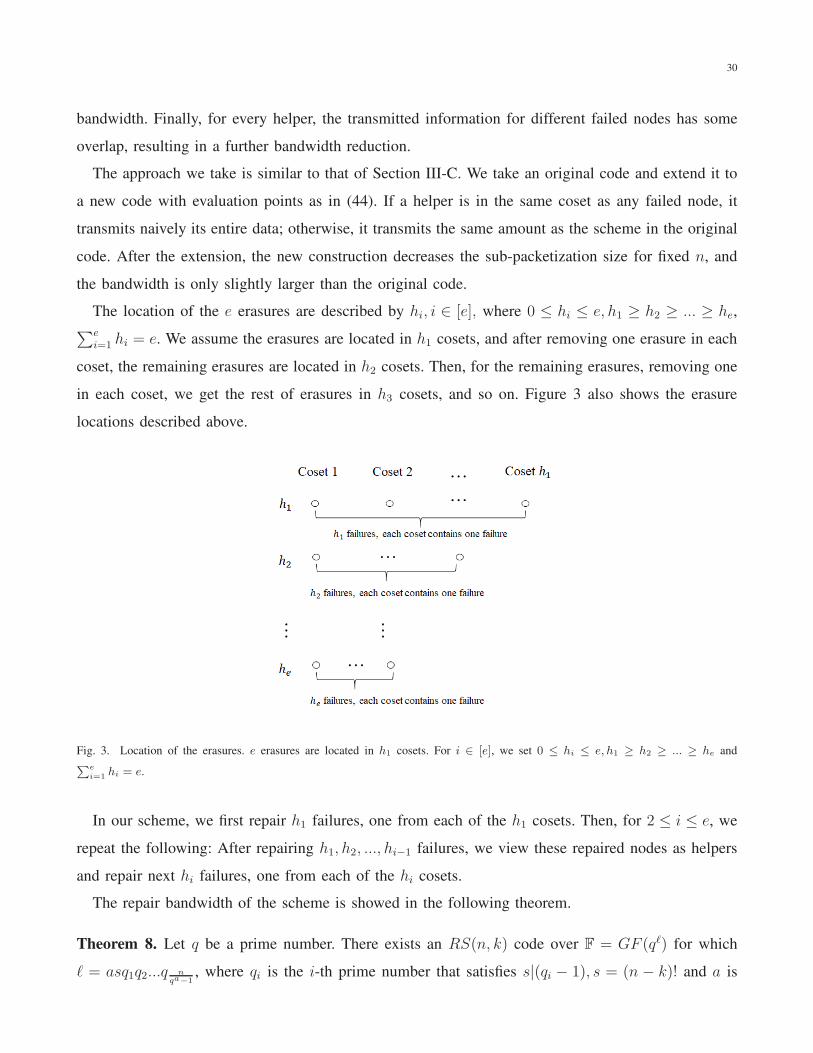
The location of the e erasures are described by hi, i ∈ [e], where 0 ≤ hi ≤ e, h1 ≥ h2 ≥ ... ≥ he,∑e

i=1 hi = e. We assume the erasures are located in h1 cosets, and after removing one erasure in each

coset, the remaining erasures are located in h2 cosets. Then, for the remaining erasures, removing one

in each coset, we get the rest of erasures in h3 cosets, and so on. Figure 3 also shows the erasure

locations described above.

Fig. 3. Location of the erasures. e erasures are located in h1 cosets. For i ∈ [e], we set 0 ≤ hi ≤ e, h1 ≥ h2 ≥ ... ≥ he and∑e

i=1 hi = e.

In our scheme, we first repair h1 failures, one from each of the h1 cosets. Then, for 2 ≤ i ≤ e, we

repeat the following: After repairing h1, h2, ..., hi−1 failures, we view these repaired nodes as helpers

and repair next hi failures, one from each of the hi cosets.

The repair bandwidth of the scheme is showed in the following theorem.

Theorem 8. Let q be a prime number. There exists an RS(n, k) code over F = GF (qℓ) for which

ℓ = asq1q2...q nqa−1

, where qi is the i-th prime number that satisfies s|(qi − 1), s = (n − k)! and a is

31

an integer. For e erasures and d helpers, e ≤ n − k, k ≤ d ≤ n − e, the average repair bandwidth

measured in symbols over B is

b ≤dℓ

(n− e)

[

(h1(qa − 1)− e) + (n− h1(q

a − 1))

e∑

i=1

hi

d− k +∑i

v=1 hv

]

, (94)

where hi, i ∈ [e] are the parameters that define the location of erasures in Fig. 3.

Proof: We first prove the case when a and ℓ′ are relatively prime using Lemma 3, the case when

a and ℓ′ are not necessarily relatively prime are proved in Appendix A. We use the code in [21]

as the original code. Let Fq(α) be the field obtained by adjoining α to the base field B = GF (q).

Similarly let Fq(α1, α2, . . . , αn) be the field for adjoining multiple elements. Let αi be an element of

order qi over B and h be the number of erasures in the original code. The original code is defined

in the field F′ = GF (qℓ

′

) = GF (qsq1q2...qn′ ), which is the degree-s of extension of Fq(α1, α2, . . . αn′).

The evaluation points are A′ = {α1, α2, . . . αn′}. The subfield F′[h] is defined as F

′[h] = Fq(αj , j =

h+ 1, h+ 2, . . . , n′), and F′i is defined as Fq(αj, j 6= i, j ∈ [n′]).

In the original code, we assume without loss of generality that there are h failed nodes f ′(α1),

f ′(α2), . . . , f′(αh). Consider the polynomials for failed node f ′(αi), 1 ≤ i ≤ h, as

p′ij(x) = xj−1g′i(x), j ∈ [si], x ∈ F′, (95)

where

g′i(x) =∏

α∈A′/(R′∪{αi,αi+1,...αh})

(x− α), x ∈ F′, (96)

for R′ ⊆ A′, |R′| = d′ being the set of helpers. The set of repair polynomials are {ηitp′ij(x), i ∈ [h], j ∈

[si], t ∈ [ sqisi]}, where ηit ∈ F

′ are constructed in [21] to ensure that {ηitp′i1(αi), ηitp

′i2(αi), . . . , ηitp

′isi(αi)}

forms the basis for F′ over F′i.

Then, the failed nodes are repaired one by one from

trF′/F′i(υαi

ηitp′ij(αi)f

′(αi)) = −n

∑

ǫ=1,ǫ 6=i

trF′/F′i(υǫηitp

′ij(αǫ)f

′(αǫ)). (97)

For x /∈ R′∪{αi, αi+1, . . . αh}, p′ij(x) = 0 and no information is transmitted. Once f ′(αi) is recovered,

it is viewed as a new helper for the failures i+ 1, i+ 2, . . . , h.

32

Since F′[h] ≤ F

′i, the information transmitted from the helper αǫ can be represented as

trF′/F′i(υǫηitp

′ij(αǫ)f

′(αǫ))

=trF′/F′i

ξ′im

q′i∑

m=1

trF′i/F′

[h](υǫηitξimp

′ij(αǫ)f

′(αǫ))

=

q′i∑

m=1

ξ′imtrF′/F′[h](υǫηitξimp

′ij(αǫ)f

′(αǫ)), (98)

where q′i =q1q2...qh

qi, {ξi1, ξi2, . . . , ξiq′i} and {ξ′i1, ξ

′i2, . . . , ξ

′iq′i} are the dual basis for F

′i over F

′[h]. We

used the fact that trF′/F′i(trF′

i/F′[h](·)) = trF′/F′

[h](·), for F′

[h] ≤ F′i ≤ F

′.

The original code satisfies the full rank condition for every i ∈ [h], and each helper αǫ transmits

[21]

rankF′[h]

(

{ηitξimp′ij(αǫ) : i ∈ [h], j ∈ [si], t ∈ [

sqisi

], m ∈ [q′i]}

)

=rankF′[h]

(

{ηitξim : i ∈ [h], t ∈ [sqisi

], m ∈ [q′i]}

)

=hℓ′

(d′ − k′ + h)∏n′

v=h+1 pv(99)

symbols over F′[h], which achieves the MSR bound.

In our new code, we extend the field to F = GF (qℓ), ℓ = aℓ′, by adjoining an order-a element αn+1

to F. We set d− k = d′ − k′. The new evaluation points consist of A = {α1E∗, α2E

∗, . . . , α′nE

∗},E =

GF (qa) = Fq(αn+1). The subfield F[h] is defined by adjoining αn+1 to F′[h], and Fi is defined as

Fq(αj, j 6= i, j ∈ [n+ 1]).

Assume first that each coset contains at most one failure, and there are h failures in total. We assume

without loss of generality that the evaluation points of the h failed nodes are in {α1E∗, α2E

∗, . . . , αhE∗},

and they are α1γ1, α2γ2, . . . , αhγh for some γw ∈ E, w ∈ [h]. Let the set of helpers be R ⊆ A, |R| = d.

We define the polynomials

pij(x) = xj−1gi(x), j ∈ [si], x ∈ F, (100)

where

gi(x) =∏

α∈A/{R∪{αiγi,αi+1γi+1,...αhγh}}

(x− α), x ∈ F. (101)

33

The set of repair polynomials are {ηitpij(x), i ∈ [h], j ∈ [si], t ∈ [ sqisi]}, where ηit ∈ F

′ are the same

as the original construction. We use field Fi as the base field for the repair.

trF/Fi(υαiγiηitpij(αiγi)f(αiγi)) = −

∑

α∈A,α6=αiγi

trF/Fi(υαηitpij(α)f(α)). (102)

If x ∈ R∪{αiγi, αi+1γi+1, . . . αhγh}, pij(x) = 0 and no information is transmitted. Next, we consider

all other nodes.

If x = αiγ for some γ ∈ E∗, we have

pij(x) = γj−1αj−1i gi(x). (103)

Since ηit, αi ∈ F′ and gi(x) is a constant independent of j, we have

rankFi({ηitpi1(x), ηitpi2(x), . . . , ηitpisi(x) : t ∈ [

sqisi

]})

=rankFi({ηit, ηitαi, . . . , ηitα

s−1i : t ∈ [

sqisi

]})

=rankF′i({ηitp

′i1(αi), ηitp

′i2(αi), . . . , ηitp

′isi(αi) : t ∈ [

sqisi

]}) (104)

which indicates the full rank. Note that the last equation follows from Lemma 3. As a result we can

recover the failed nodes and each helper in the cosets containing the failed nodes transmit ℓ symbols

in B.

For x = αǫγ, ǫ > h, since F[h] is a subfield of Fi and from Lemma 3 we know that {ξi1, ξi2, . . . , ξiq′i}

and {ξ′i1, ξ′i2, . . . , ξ

′iq′i} are also the dual basis for Fi over F[h], then, similar to (98), we have

trF/Fi(υαηitpij(x)f(x)) =

q′i∑

m=1

ξ′imtrF/F[h](υǫηitξimpij(x)f(x)). (105)

Using the fact that gi(x) is a constant independent of j, x ∈ F[h] and ηitξim ∈ F′, from Lemma 3 we

know that

rankF[h]

(

{ηitξimpij(x) : i ∈ [h], j ∈ [si], t ∈ [sqisi

], m ∈ [q′i]}

)

=rankF[h]

(

{ηitξim : i ∈ [h], t ∈ [sqisi

], m ∈ [q′i]}

)

=rankF′[h]

(

{ηitξim : i ∈ [h], t ∈ [sqisi

], m ∈ [q′i]}

)

=rankF′[h]

(

{ηitξimp′ij(αǫ) : i ∈ [h], j ∈ [si], t ∈ [

sqisi

], m ∈ [q′i]}

)

=hℓ′

(d− k + h)∏n′

v=h+1 qv, (106)

34

where the last equality follows from (99) and d′ − k′ = d − k. So, each helper in the other cosets

transmits hℓd−k+h

symbols over B.

Using the above results, we calculate the repair bandwidth in two steps.

Step 1. We first repair h1 failures, one from each of the h1 cosets. From (104), we know that in the h1

cosets containing the failed nodes, we transmit ℓ symbols over B. By (106), for each helper in other

cosets, we transmit h1ℓd−k+h1

symbols over B.

Step 2. For 2 ≤ i ≤ e, repeat the following. After repairing h1, h2, ..., hi−1 failures, these nodes can be

viewed as helpers for repairing next hi failures, one from each of the hi cosets. So, we have d+i−1∑

v=1

hv

helpers for the hi failures. For the helpers in the h1 cosets containing the failed nodes, we already

transmit ℓ symbols over B in Step 1 and no more information needs to be transmitted. For each helper

in other cosets, we transmit hiℓ

d−k+∑i

v=1 hvsymbols over B.

Thus, we can repair all the failed nodes. The repair bandwidth can be calculated as (94).

Suppose that e failures are to be recovered. Compared to the naive strategy which always uses

d helpers to repair the failures one by one, our scheme gets a smaller repair bandwidth since the

recovered failures are viewed as new helpers and we take advantage of the overlapped symbols for

repairing different failures similar to [21].

In the case when n ≫ e(qa − 1), or when we arrange nodes with correlated failures in different

cosets, we can assume that all the erasures are in different cosets, h1 = e, h2 = h3 = ... = he = 0. For

example, if correlated failures tend to appear in the same rack in a data center, we can assign each

node in the rack to a different coset. Under such conditions, we simplify the repair bandwidth as

b ≤d

n− e

eℓ

d− k + e(n− e+ (d− k)(qa − 2)). (107)

Indeed, one can examine the expression of (94). With the constraint that∑e

i=1 hi = e, the first term

h1(qa−1)− e) is an increasing function of h1 and the second term (n−h1(q

a−1))∑e

i=1hi

d−k+∑i

v=1 hv

is a decreasing function of h1. Under the assumption that n is large, the second term dominates,

and increasing h1 reduces the total repair bandwidth b. Namely, h1 = e corresponds to the lowest

bandwidth for large code length.

In particular, when d = n− e, h1 = e, we have

b =eℓ

n− k(n− e) +

eℓ

n− k(n− k − e)(qa − 2), (108)

where the second term is the extra repair bandwidth compared with the MSR bound.

35

TABLE III

Repair bandwidth of different schemes for e erasures.

repair bandwidth number of helpers

Single-erasure repair

in one coset (separate repair)

eℓa(n− 1)(a− s) n− 1

Multiple-erasure repair

in one coset (simultaneous repair)

eℓa(n− e)(a− s) n− e

Single-erasure repair

in multiple cosets (separate repair)

eℓn−k

[n− 1 + (n− k − 1)(qa − 2)] n− 1

Multiple-erasure repair

in multiple cosets (simultaneous repair)

eℓn−k

[n− e+ (n− k − e)(qa − 2)] n− e

D. Numerical evaluations and discussions

In this subsection, we compare our schemes for multiple erasures with previous results, including

separate repair and schemes in [18] and [21].

We first demonstrate that repairing multiple erasures simultaneously can save repair bandwidth

compared to repairing erasures separately. Let us assume e failures happen one by one, and the rest of

n− 1 nodes are available as helpers initially when the first failure occurs. We can either repair each

failure separately using n−1 helpers, or wait for e failures and repair all of them simultaneously with

n − e helpers. Table III shows the comparison. For our scheme in one coset, separate repair needs

a repair bandwidth of eℓa(n − 1)(a − s) symbols in B, simultaneous a repair requires bandwidth of

eℓa(n − e)(a − s). For our scheme in multiple cosets, we can repair the failures separately by n − 1

helpers with the bandwidth of eℓn−k

[n− 1+ (n− k− 1)(qa − 2)], and with simultaneous repair we can

achieve the bandwidth of eℓn−k

[n − e + (n − k − e)(qa − 2)]. One can see that in both constructions,

simultaneous repair outperforms separate repair.

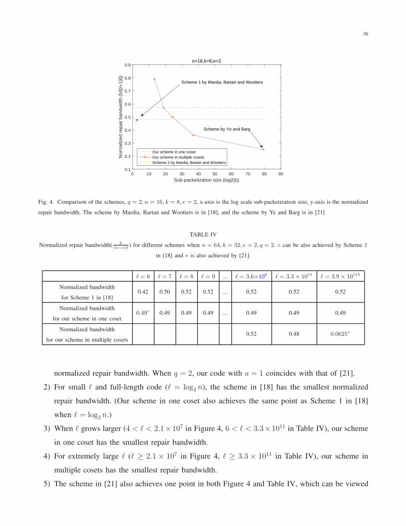
Nest we compare our scheme for multiple erasures with the existing schemes. Figure 4 shows the

normalized repair bandwidth for different schemes when n = 16, k = 8, e = 2, q = 2. Table IV shows

the comparison when n = 64, k = 32, e = 2, q = 2. We make the following observations:

1) For fixed (n, k) and our scheme with multiple cosets, we use the paremeter a to adjust the

sub-packetization size. From Theorem 8, we know that ℓ ≈ a · ( nqa−1

)(n

qa−1), which means that

increasing a will decrease the sub-packetization ℓ. In our schemes with one coset and two cosets,

the parameter a is determined by the code length n, so increasing ℓ will not change a or the

36

0 10 20 30 40 50 60 70 80 90

Sub-packetization size (log2(l))

0.1

0.2

0.3

0.4

0.5

0.6

0.7

0.8

0.9

Nor

mal

ized

rep

air

band

wid

th (

b/[(

n-1)

l])

n=16,k=8,e=2

o

Our scheme in one cosetOur scheme in multiple cosetsScheme 2 by Mardia, Bartan and Wootters

Scheme by Ye and Barg

Scheme 1 by Mardia, Bartan and Wootters

Fig. 4. Comparison of the schemes, q = 2, n = 16, k = 8, e = 2, x-axis is the log scale sub-packetization size, y-axis is the normalized

repair bandwidth. The scheme by Mardia, Bartan and Wootters is in [18], and the scheme by Ye and Barg is in [21]

TABLE IV

Normalized repair bandwidth( b(n−e)ℓ

) for different schemes when n = 64, k = 32, e = 2, q = 2. ◦ can be also achieved by Scheme 1

in [18] and ∗ is also achieved by [21].

ℓ = 6 ℓ = 7 ℓ = 8 ℓ = 9 ... ℓ = 3.6×106 ℓ = 3.3× 1011 ℓ = 3.9× 10115

Normalized bandwidth

for Scheme 1 in [18]0.42 0.50 0.52 0.52 ... 0.52 0.52 0.52

Normalized bandwidth

for our scheme in one coset0.49◦ 0.49 0.49 0.49 ... 0.49 0.49 0.49

Normalized bandwidth

for our scheme in multiple cosets0.52 0.48 0.0625∗

normalized repair bandwidth. When q = 2, our code with a = 1 coincides with that of [21].

2) For small ℓ and full-length code (ℓ = log2 n), the scheme in [18] has the smallest normalized

repair bandwidth. (Our scheme in one coset also achieves the same point as Scheme 1 in [18]

when ℓ = log2 n.)

3) When ℓ grows larger (4 < ℓ < 2.1×107 in Figure 4, 6 < ℓ < 3.3×1011 in Table IV), our scheme

in one coset has the smallest repair bandwidth.

4) For extremely large ℓ (ℓ ≥ 2.1 × 107 in Figure 4, ℓ ≥ 3.3 × 1011 in Table IV), our scheme in

multiple cosets has the smallest repair bandwidth.

5) The scheme in [21] also achieves one point in both Figure 4 and Table IV, which can be viewed

37

as a special case of our scheme in multiple cosets.

V. CONCLUSION

In this paper, we designed three Reed-Solomon code repair schemes to provide a tradeoff between

the sub-packetization size and the repair bandwidth. Our schemes choose the evaluation points of the

Reed-Solomon code from one, two, or multiple cosets of the multiplicative group of the underlying

finite field. For a single erasure, when the sub-packetization size is large, the scheme in multiple

cosets has better performance, it approaches the MSR bound. When sub-packetization size is small,

the scheme in one coset has advantages in repair bandwidth. The scheme in two cosets has smaller

repair bandwidth with certain parameters in between the other two cases. For multiple erasures, our

scheme in one coset has constructions for arbitrary redundancy n − k and our scheme in multiple

cosets reduced the sub-packetization size of an MSR code. The two schemes together provided a set

of tradeoff points and we observe similar tradeoff characteristics as in the single erasure case. In spite

of several tradeoff points we provided in this paper, the dependence of the sub-packetization size

versus the repair bandwidth is still an open question.

APPENDIX A

PROOF OF SCHEMES IN MULTIPLE COSETS FOR THE CASE OF ARBITRARY a AND ℓ′

In this section, we first introduce a lemma similar to Lemma 3 that does not require a and ℓ′ to be

relatively prime. By applying this lemma, our constructions in multiple cosets for single and multiple

erasures can be generalized when a and ℓ′ are arbitrary integers.

We note that a finite field F = GF (qℓ) is also a vector space over GF (q). Let E be a sub-

space of F. Define the subspace spanned by a set of elements {γ1, γ2, . . . , γi} ⊆ F over E as

spanE{γ1, γ2, . . . , γi} , {

∑ij=1 bjγj : bj ∈ E}. The rank rankE({γ1, γ2, ..., γi}) is defined to be

the cardinality of a maximal subset of {γ1, γ2, ..., γi} that is linearly independent over E.

Lemma 6. Let B = GF (q),F′ = GF (qℓ′

), F = GF (qℓ), ℓ = aℓ′, and q be any power of a prime

number. Define the subspace E = spanB{β1, β2, . . . , βa}, where {β1, β2, . . . , βa} is a basis for F over

F′. For any set of {γ1, γ2, ..., γℓ′} ⊆ F

′ ≤ F, we have

rankE({γ1, γ2, ..., γℓ′})

=rankB({γ1, γ2, ..., γℓ′}). (109)

38

Proof: Assume rankB({γ1, γ2, ..., γℓ′}) = c and without loss of generality, {γ1, γ2, ..., γc} are lin-

early independent over B. Then, we can construct {γ′c+1, γ

′c+2, ..., γ

′ℓ′} ⊆ F

′ to make {γ1, γ2, ..., γc, γ′c+1,

γ′c+2, ..., γ

′ℓ′} form a basis for F′ over B.

Since {β1, β2, . . . , βa} is the basis for F over F′, we know that {βiγ1, βiγ2, ..., βiγc, βiγ′c+1,βiγ

′c+2, ...,

βiγ′ℓ′ : i ∈ [a]} is the basis for F over B. Then, we have F = span

E{γ1, γ2, ..., γc, γ

′c+1, γ

′c+2, ..., γ

′ℓ′},

namely, {γ1, γ2, ..., γc, γ′c+1, γ

′c+2, ..., γ

′ℓ′} is a basis for F over E, hence {γ1, γ2, ..., γc} are linearly

independent over E,

rankE({γ1, γ2, ..., γℓ′})

≥c

=rankB({γ1, γ2, ..., γℓ′}). (110)

Since B ⊆ E, we also have

rankE({γ1, γ2, ..., γℓ′})

≤rankB({γ1, γ2, ..., γℓ′}). (111)

The proof is completed.

For the schemes in multiple cosets when a and ℓ′ are not relatively prime, we just use the subspace

E = spanB{β1, β2, ..., βa} to replace the subfield GF (qa). We denote by E

∗ = E\{0} for the subspace

E. The evaluation points of the new code are {γE∗ : γ ∈ A′} where A′ ⊆ F′ is the set of evaluation

points for the original code. In the proofs, we use Lemma 6 instead of Lemma 3. For example, from

Lemma 6 we know that the new evaluation points are all distinct if the elements in A′ are linearly

independent over B.

APPENDIX B

PROOF OF THEOREM 6

In this section, we prove the equivalence of Definitions 1 and 2. We first show that the dual code

scheme in Definition 2 reduces to a linear repair scheme as in Definition 1 in Lemma 7. Then, we

show that Definition 1 reduces to Definition 2 in Lemma 8 and Lemma 9.

Lemma 7. The dual code scheme can be reduced to the linear repair scheme in Definition 1.

39

Proof: In the dual code scheme, we repair nodes [e] from the linearly independent equations

e∑

v=1

trF/B(C′ijvCv) = −

n∑

t=e+1

trF/B(C′ijtCt), i ∈ [e], j ∈ [ℓ]. (112)

Here, C ′ijt can be written as

C ′ijt =

ℓ∑

m=1

ξ′mtrF/B(ξmC′ijt), (113)

where {ξ1, ξ2, . . . , ξℓ} and {ξ′1, ξ′2, . . . , ξ

′ℓ} are the dual basis for F over B. Then, we can rewrite (112)

in matrix form as

e∑

v=1

Siv

trF/B(ξ′1Cv)

trF/B(ξ′2Cv)

...

trF/B(ξ′ℓCv)

= −n

∑

t=e+1

Sit

trF/B(ξ′1Cv)

trF/B(ξ′2Cv)

...

trF/B(ξ′ℓCv)

, i ∈ [e], (114)

where Sit ∈ Bℓ×ℓ is called the repair matrix defined as

Sit =

trF/B(ξ1C′i1t) · · · trF/B(ξℓC

′i1t)

trF/B(ξ1C′i2t) · · · trF/B(ξℓC

′i2t)

.... . .

...

trF/B(ξ1C′iℓt) · · · trF/B(ξℓC

′iℓt)

, (115)

Let

Xw ,

trF/B(ξ′1Cw)

trF/B(ξ′2Cw)

...

trF/B(ξ′ℓCw)

, w ∈ [n]. (116)

We want to solve Xi, i ∈ [e], which can be used to recover the e failed nodes C1, C2, . . . , Ce. Define

matrix S as

S =

S11 S12 · · · S1e

S21 S22 · · · S2e

......

. . ....

Se1 Se2 · · · See

. (117)

40

Then, (114) can be represented as

S

X1

X2

...

Xe

= −n

∑

t=e+1

S1t

S2t

...

Set

Xt. (118)

Thus, from Lemma 4 we know that if the full rank condition satisfies1, S has full rank so we can

solve Xi, i ∈ [e]. Then, Ci, i ∈ [e] can be repaired from

Ci =

ℓ∑

m=1

ξmtrF/B(ξ′mCi), (119)

Now, set µim = ξm, we get λim = trF/B(ξ′mCi), which can be solved from (118). Note that the right

side of (118) is equal to the right side of (112), we get the queries Qt = {C ′ijt, i ∈ [e], j ∈ [ℓ]} and

the coefficients βimγt come from matrix S.

Then, we can get the repair bandwidth condition:

b =

n∑

t=e+1

rankB({C′ijt : i ∈ [e], j ∈ [ℓ]}) =

ℓ∑

t=e+1

rankB(Qt). (120)

Lemma 8. A linear repair scheme in Definition 1 can be represented in the form below:

µ′ijCi =

n∑

t=e+1

θijtCt, i ∈ [e], j ∈ [ℓ], (121)

where {µ′i1, µ

′i2, ..., µ

′iℓ} is the dual basis of {µi1, µi2, ..., µiℓ}, and θijt ∈ span

B(Qt), e+1 ≤ t ≤ n, i ∈

[e], j ∈ [ℓ] are some coefficients in F. The repair bandwidth is

b =n

∑

t=e+1

rankB({θijt : i ∈ [e], j ∈ [ℓ]}). (122)

Proof: By (67) and (68) we have

n∑

t=e+1

∑

γ∈Qt

trF/B(βijγt · γCt) = λij = trF/B(µ′ijCi). (123)

1We use Lemma 4 while in Lemma 4 we use the polynomials pij(x) as part of the elements in the defined matrix Sit. However, in

Lemma 4 we just view the polynomials pij(x) as a symbol, change them to the dual codeword symbol C′ijt will not have effects on

the results of the lemma.

41

Set θijt =∑

γ∈Qtβijγt · γ. Then, we have θijt ∈ span

B(Qt). Hence,

n∑

t=e+1

trF/B(θijtCt) =n

∑

t=e+1

trF/B(∑

γ∈Qt

βijγt · γCt) = trF/B(µ′ijCi). (124)

Equations (123) and (124) hold for all f ∈ F[x]. Since the RS code is a linear code, they also hold

for δm · f ∈ F[x] for all δm ∈ F. In particular, let δm, m ∈ [ℓ], be a basis for F over B, Then,

trF/B(δm · µ′ijCi) = trF/B(δm ·

n∑

t=e+1

θijtCt), ∀m ∈ [ℓ], (125)

which in turn implies that θijt also satisfies (121).

Note that the repair bandwidth (122) also satisfies

b =

n∑

t=e+1

rankB(θijt : i ∈ [e], j ∈ [ℓ])

≤

n∑

t=e+1

rankB(Qt), (126)

since θijt ∈ spanB(Qt). However, for any linear scheme L in Definition 1, if (126) holds with strict

inequality, we can improve the linear scheme L by setting Qt such that spanB(Qt) = span

B({θijt, i ∈

[e], j ∈ [ℓ]}), for all e + 1 ≤ t ≤ n. Hence, the linear scheme L and the scheme in Lemma 8 have

identical bandwidth.

Lemma 9. The scheme in Lemma 8 can be represented by the dual code scheme in Definition 2.

Proof: By (121), (0, . . . , µ′ij, . . . , 0, θije+1, . . . , θijn) is a dual codeword, where µ′

ij is the i-th entry.

Then, for j ∈ [ℓ], we set C ′ijt such that C ′

iji = −µ′ij , C

′ijv = 0, v ∈ [e], v 6= i and C ′

ijt = θijt, e + 1 ≤

t ≤ n. The full rank condition follows because {µ′i1, µ

′i2, ..., µ

′iℓ} is the basis for F over B, and the

repair bandwidth condition follows from (126). Thus, we obtain the dual code scheme in Definition

2.

APPENDIX C

PROOF OF LEMMA 4

Proof: Vectors Vij, i ∈ [e], j ∈ [ℓ] are linearly independent over B is equivalent to that there is no

nonzero bij ∈ B, i ∈ [e], j ∈ [ℓ] that satisfy

∑

i,j

bijpij(αv) = 0, ∀v ∈ [e]. (127)

42

Here, pij(x) can be written as

pij(x) =ℓ

∑

m=1

ξ′mtrF/B(ξmpij(x)), (128)

where {ξ1, ξ2, . . . , ξℓ} and {ξ′1, ξ′2, . . . , ξ

′ℓ} are the dual basis for F over B. So, it is equivalent to that

there is no nonzero bij ∈ B, i ∈ [e], j ∈ [ℓ] that satisfy

∑

i,j

bij

ℓ∑

m=1

ξ′mtrF/B(ξmpij(αv)) = 0, ∀v ∈ [e]. (129)

Since {ξ′1, ξ′2, . . . , ξ

′ℓ} are linearly independent over B. Therefore, there is no nonzero bij ∈ B, i ∈

[e], j ∈ [ℓ] that satisfy

∑

i,j

bijtrF/B(ξmpij(αv)) = 0, ∀v ∈ [e], m ∈ [ℓ], (130)

which is equivalent to S has full rank.

APPENDIX D

PROOF OF LEMMA 5

Proof: Assume rankB({pij(αt), i ∈ [e], j ∈ [ℓ]}) = c and {pij(αt), (i, j) ∈ I} are linearly inde-

pendent over B, |I| = c. Define Sit(j) as the vector for the j-th row in Sit: Sit(j) = (trF/B(ξ1pij(αt)),

trF/B(ξ2pij(αt)), ..., trF/B(ξℓpij(αt))). We first prove {Sit(j), (i, j) ∈ I} are linearly independent and

then prove Si′t(j′), i′ ∈ [e], j′ ∈ [ℓ], (i′, j′) /∈ I can be represented as B-linear combinations of

{Sit(j), (i, j) ∈ I} .

If {Sit(j), (i, j) ∈ I} are linearly dependent over B, then there exists some nonzero bij ∈ B, (i, j) ∈ I

that satisfies

∑

(i,j)∈I

bijSit(j) = 0, (131)

and we have

∑

(i,j)∈I

bijtrF/B(ξmpij(αt)) = 0, ∀m ∈ [ℓ]. (132)

Multiplying the above equation by ξ′m and summing over all m ∈ [ℓ] result in

∑

(i,j)∈I

ℓ∑

m=1

bijξ′mtrF/B(ξmpij(αt)) = 0. (133)

43

Then, from (128) we know that bij satisfies

∑

(i,j)∈I

bijpij(αt) = 0, (134)

which is contradictory to the statement that {pij(αt), (i, j) ∈ I} are linearly independent over B.

Therefore, {Sit(j), (i, j) ∈ I} are linearly independent over B.

Let us assume pi′j′(αt), i′ ∈ [e], j′ ∈ [ℓ], (i′, j′) /∈ I can be represented as

pi′j′(αt) =∑

(i,j)∈I

b′ijpij(αt), for some b′ij ∈ B. (135)

Then, for m ∈ [ℓ],

trF/B(ξmpi′j′(αt)) = trF/B

ξm∑

(i,j)∈I

b′ijpij(αt)

=∑

(i,j)∈I

b′ijtrF/B(ξmpij(αt)), (136)

which means that for i′ ∈ [e], j′ ∈ [ℓ], (i′, j′) /∈ I ,

Si′t(j′) =

∑

(i,j)∈I

b′ijSit(j) (137)

is the B-linear combination of {Sit(j), (i, j) ∈ I}.

REFERENCES

[1] F. J. MacWilliams and N. J. A. Sloane, The theory of error-correcting codes. Elsevier, 1977.

[2] W. Ryan and S. Lin, Channel codes: classical and modern. Cambridge University Press, 2009.

[3] V. Guruswami and M. Sudan, “Improved decoding of Reed-Solomon and algebraic-geometric codes,” in Foundations of Computer

Science, 1998. Proceedings. 39th Annual Symposium on. IEEE, 1998, pp. 28–37.

[4] K. Shanmugam, D. S. Papailiopoulos, A. G. Dimakis, and G. Caire, “A repair framework for scalar MDS codes,” IEEE Journal

on Selected Areas in Communications, vol. 32, no. 5, pp. 998–1007, 2014.

[5] V. Guruswami and M. Wootters, “Repairing Reed-Solomon codes,” IEEE Transactions on Information Theory, 2017.

[6] H. Dau and O. Milenkovic, “Optimal repair schemes for some families of full-length Reed-Solomon codes,” in Information Theory

(ISIT), 2017 IEEE International Symposium on. IEEE, 2017, pp. 346–350.

[7] A. G. Dimakis, P. B. Godfrey, Y. Wu, M. J. Wainwright, and K. Ramchandran, “Network coding for distributed storage systems,”

IEEE Transactions on Information Theory, vol. 56, no. 9, pp. 4539–4551, 2010.

[8] K. V. Rashmi, N. B. Shah, and P. V. Kumar, “Optimal exact-regenerating codes for distributed storage at the MSR and MBR

points via a product-matrix construction,” IEEE Transactions on Information Theory, vol. 57, no. 8, pp. 5227–5239, 2011.

[9] D. S. Papailiopoulos, A. G. Dimakis, and V. R. Cadambe, “Repair optimal erasure codes through hadamard designs,” IEEE Trans.

Inf. Theory, vol. 59, no. 5, pp. 3021–3037, 2013.

[10] I. Tamo, Z. Wang, and J. Bruck, “Zigzag codes: MDS array codes with optimal rebuilding,” IEEE Trans. Inf. Theory, vol. 59,

no. 3, pp. 1597–1616, March 2013.

44

[11] Z. Wang, I. Tamo, and J. Bruck, “Explicit minimum storage regenerating codes,” IEEE Transactions on Information Theory,

vol. 62, no. 8, pp. 4466–4480, Aug 2016.

[12] A. S. Rawat, O. O. Koyluoglu, and S. Vishwanath, “Progress on high-rate MSR codes: Enabling arbitrary number of helper nodes,”

in Information Theory and Applications Workshop (ITA), 2016. IEEE, 2016, pp. 1–6.

[13] S. Goparaju, A. Fazeli, and A. Vardy, “Minimum storage regenerating codes for all parameters,” IEEE Transactions on Information

Theory, vol. 63, no. 10, pp. 6318–6328, 2017.

[14] M. Ye and A. Barg, “Explicit constructions of optimal-access MDS codes with nearly optimal sub-packetization,” IEEE Transactions

on Information Theory, vol. 63, no. 10, pp. 6307–6317, Oct 2017.

[15] ——, “Explicit constructions of MDS array codes and RS codes with optimal repair bandwidth,” in Information Theory (ISIT),

2016 IEEE International Symposium on. IEEE, 2016, pp. 1202–1206.

[16] I. Tamo, M. Ye, and A. Barg, “Optimal repair of Reed-Solomon codes: achieving the cut-set bound,” arXiv preprint

arXiv:1706.00112, 2017.

[17] H. Dau, I. Duursma, H. M. Kiah, and O. Milenkovic, “Repairing reed-solomon codes with multiple erasures,” IEEE Transactions

on Information Theory, 2018.

[18] J. Mardia, B. Bartan, and M. Wootters, “Repairing multiple failures for scalar MDS codes,” IEEE Transactions on Information

Theory, 2018.

[19] M. Zorgui and Z. Wang, “Centralized multi-node repair regenerating codes,” IEEE Transactions on Information Theory, 2019.

[20] ——, “On the achievability region of regenerating codes for multiple erasures,” in 2018 IEEE International Symposium on

Information Theory (ISIT). IEEE, 2018, pp. 2067–2071.

[21] M. Ye and A. Barg, “Repairing Reed-Solomon codes: universally achieving the cut-set bound for any number of erasures,” arXiv

preprint arXiv:1710.07216, 2017.

[22] S. B. Gashkov and I. S. Sergeev, “Complexity of computation in finite fields,” Journal of Mathematical Sciences, vol. 191, no. 5,

pp. 661–685, 2013.

[23] K. M. Greenan, E. L. Miller, and S. T. J. Schwarz, “Optimizing galois field arithmetic for diverse processor architectures and

applications,” in Modeling, Analysis and Simulation of Computers and Telecommunication Systems, 2008. MASCOTS 2008. IEEE

International Symposium on. IEEE, 2008, pp. 1–10.

[24] J. S. Plank, K. M. Greenan, and E. L. Miller, “Screaming fast galois field arithmetic using intel simd instructions.” in FAST, 2013,

pp. 299–306.

[25] J. Luo, K. D. Bowers, A. Oprea, and L. Xu, “Efficient software implementations of large finite fields GF(2n) for secure storage

applications,” ACM Transactions on Storage (TOS), vol. 8, no. 1, p. 2, 2012.

[26] J. S. Plank, J. Luo, C. D. Schuman, L. Xu, Z. Wilcox-O’Hearn et al., “A performance evaluation and examination of open-source

erasure coding libraries for storage.” in Fast, vol. 9, 2009, pp. 253–265.

[27] V. Guruswami and A. S. Rawat, “MDS code constructions with small sub-packetization and near-optimal repair bandwidth,” in

Proceedings of the Twenty-Eighth Annual ACM-SIAM Symposium on Discrete Algorithms. Society for Industrial and Applied

Mathematics, 2017, pp. 2109–2122.

[28] O. Khan, R. C. Burns, J. S. Plank, W. Pierce, and C. Huang, “Rethinking erasure codes for cloud file systems: minimizing I/O

for recovery and degraded reads.” in FAST, 2012, p. 20.

[29] J. Li and X. Tang, “A systematic construction of mds codes with small sub-packetization level and near optimal repair bandwidth,”

arXiv preprint arXiv:1901.08254, 2019.

[30] K. Kralevska, D. Gligoroski, R. E. Jensen, and H. Øverby, “HashTag erasure codes: from theory to practice,” IEEE Transactions

on Big Data, vol. 4, no. 4, pp. 516–529, 2018.

45

[31] A. Chowdhury and A. Vardy, “Improved schemes for asymptotically optimal repair of MDS codes,” arXiv preprint

arXiv:1710.01867, 2017.

[32] M. Sathiamoorthy, M. Asteris, D. Papailiopoulos, A. G. Dimakis, R. Vadali, S. Chen, and D. Borthakur, “Xoring elephants: Novel

erasure codes for big data,” in Proceedings of the VLDB Endowment, vol. 6, no. 5. VLDB Endowment, 2013, pp. 325–336.

[33] V. R. Cadambe, S. A. Jafar, H. Maleki, K. Ramchandran, and C. Suh, “Asymptotic interference alignment for optimal repair of

MDS codes in distributed storage,” IEEE Transactions on Information Theory, vol. 59, no. 5, pp. 2974–2987, 2013.

[34] D. Goss, Basic structures of function field arithmetic. Springer Science & Business Media, 2012.

[35] R. Lidl and H. Niederreiter, Introduction to finite fields and their applications. Cambridge university press, 1994.