on the use of advanced pattern recognition techniques for ... · para la aplicación de técnicas...

Universitat Autònoma de Barcelona

Department of Information and Communications Engineering

On the Use of Advanced Pattern Recognition

Techniques for the Analysis of MRS and MRSI

Data in Neuro-Oncology

by

Sandra Ortega-Martorell

A thesis submitted in partial fulfilment

for the degree of Doctor in Computer Science

Advisors

Dr. Alfredo Vellido, Universitat Politècnica de Catalunya Prof. Paulo J.G. Lisboa, Liverpool John Moores University

Prof. Carles Arús, Universitat Autònoma de Barcelona

Tutor

Dr. Joan Borrell, Universitat Autònoma de Barcelona

May, 2012

i

On the Use of Advanced Pattern Recognition Techniques for the Analysis of MRS and MRSI Data in Neuro-Oncology


Thesis summary

Cancer is a leading cause of death worldwide. Tumours of the Central Nervous System and, among them, brain tumours have a relatively low incidence as compared to other more widespread cancer pathologies, but the prognosis of some of them is very poor, contributing significantly to morbidity. The clinical management of an abnormal mass in the brain is sensitive and difficult, making experts to rely on non-invasive indirect measurements of the tumour characteristics and growth. In current radiological practice, these data measurements are often provided by magnetic resonance (MR) techniques, such as imaging (MRI) and spectroscopy (MRS). The rich information contained in MR signals makes them ideally suited to the application of pattern recognition (PR) techniques. Over the last two decades, these techniques have been successfully used to address the problem of knowledge extraction from human brain tumour data, for their diagnosis and prognosis. Nevertheless, the discrimination of some tumour types and subtypes, along with the accurate delimitation of the tumour area, remained challenging. In this thesis, we approach these challenges using a set of advanced PR techniques. A variety of common and well-known dimensionality reduction (DR), classification, and evaluation methods are first gathered in a software tool, used for the development of classifiers that are suitable for the analysis of MRS data. We then delve into the feature extraction (FE) family of DR methods to propose a method that is robust in the presence of noise, not prone to overfitting, and which also provides interpretation of the extracted MRS signal prototypes. Two spectral decomposition techniques, in different algorithmic variants, are subsequently used to extract the sources of the MRS signals and identify the one that provides better results in the context of neuro-oncology, using single-voxel (SV) MRS data. The best and most adequate source extraction method is then used to derive sources correlated with the mean spectra of known tissue types. Its accuracy for class assignment when sources are used directly for classification is assessed, as well as when used for DR prior to classification. The former, an unsupervised approach, is also applied in this thesis in the multi-voxel (MV) context, where we propose a mechanism for delimiting the pathological area of the tumour. The contributions of this thesis can be summarised as follows. First, the development of a software tool allowed us to reproduce previously published MRS-based classifiers, and test new hypotheses that led to new publications. We also contributed a FE method, whose performance is comparable to its most commonly used counterpart in MRS data analysis, while improving on the interpretability. Moreover, we identified, after an exhaustive evaluation, the spectral decomposition variant that best suits the analysis of SV MRS data, namely Convex Non-negative Matrix Factorisation (NMF), and showed its ability to discriminate between healthy tissue, necrosis, and actively proliferating tumour, with results that are comparable to those obtained in fully supervised mode. The use of the extracted sources for DR leads to simple classifiers with independent test performances that are comparable with, and are often better

ii

than, previously described strategies. For MV data, we successfully benchmarked alternative spectral decomposition methods, and provided evidence supporting that very accurate delimitation can be achieved through the application of Convex-NMF. With this thesis, we provide spectroscopists with a tool that facilitates the development of classifiers for the analysis of MRS data, for a large group of tumour types; allowing them to concentrate on the interpretation of the results, without requiring a specialised mathematical expertise for testing their hypotheses. We also provide an unsupervised alternative to improve the discrimination between tumour types and subtypes, placing this approach one step ahead of classical label-requiring supervised methods for detection of the increasingly recognised molecular subtype heterogeneity within human brain tumours. This also allowed us to accurately tackle one of the main sources of uncertainty in the clinical management of brain tumours, which is the difficulty of appropriately delimiting the pathological area.

iii

On the Use of Advanced Pattern Recognition Techniques for the Analysis of MRS and MRSI Data in Neuro-Oncology


Resumen de la tesis

El cáncer es una de las principales causas de muerte en el mundo. Los tumores del sistema nervioso central y, de entre ellos, los tumores cerebrales, tienen una incidencia relativamente baja en comparación con otras patologías cancerígenas más generalizadas, pero la prognosis de algunos de los mismos es muy pobre, lo cual contribuye significativamente a su morbilidad. La gestión clínica de una masa anormal en el cerebro es materia delicada y difícil, por lo que los expertos han de basarse en mediciones indirectas no invasivas de las características del tumor y de su crecimiento. En la práctica radiológica de hoy en día, estas mediciones se realizan a menudo mediante técnicas de resonancia magnética (MR), como la imagen (MRI) y la espectroscopia (MRS). La vasta información contenida en las señales de MR les hace ideales para la aplicación de técnicas de reconocimiento de patrones (PR). A lo largo de las dos últimas décadas, estas técnicas se han aplicado con éxito al problema de la extracción de conocimiento a partir de datos de tumores cerebrales humanos, para su diagnóstico y pronóstico. No obstante, la discriminación de algunos tipos y subtipos de tumores, así como la delimitación precisa del área tumoral, continúan siendo un reto para los investigadores. En esta tesis, abordamos tales retos mediante la aplicación de un conjunto de técnicas avanzadas de PR. En primera instancia, se implementaron una variedad de técnicas comunes y bien conocidas en una herramienta integrada de software. Esta fue utilizada en tareas de reducción de dimensionalidad (DR), clasificación y evaluación de modelos, dentro del objetivo general de desarrollar clasificadores apropiados para el análisis de datos de MRS. Posteriormente, se profundizó en el desarrollo de métodos de extracción de características (FE), perteneciente a la familia de métodos de DR, para proponer un método que es robusto en presencia de ruido, no propenso a sobreajuste, y que también proporciona prototipos de señal interpretables a partir de los datos de MRS. En una siguiente fase, dos técnicas de descomposición espectral, en diferentes variantes algorítmicas, fueron utilizadas para extraer las fuentes de señal de MRS e identificar la que proporciona mejores resultados en el contexto de problemas de neuro-oncología, utilizando datos de MRS de un solo vóxel (SV). El mejor y más adecuado método de extracción de fuentes resultante se utilizó posteriormente para derivar fuentes correlacionadas con los espectros promedio de los tipos de tejidos estudiados. Su precisión para la asignación de clases fue evaluada tanto cuando las fuentes se utilizan directamente para la clasificación, como cuando se utilizan para DR previa a la clasificación. El primer enfoque, no supervisado, se aplica también en esta tesis en el contexto de datos de múltiples vóxeles (MV), donde se propone un mecanismo para la delimitación de la zona patológica del tumor. Las contribuciones de esta tesis se pueden resumir de la siguiente manera. En primer lugar, el desarrollo de una herramienta de software que ha permitido reproducir clasificadores previamente publicados, basados en datos de MRS, así como probar nuevas hipótesis que dieron lugar a nuevas publicaciones. También se ha contribuido con un método de FE, cuyo rendimiento es comparable a su contraparte más comúnmente utilizada en el análisis de datos de MRS, al tiempo que mejora su interpretación. Por otra parte, hemos identificado, después de

iv

una exhaustiva evaluación, la variante de descomposición espectral que mejor se adapta al análisis de datos de SV MRS, llamada Convex Non-negative Matrix Factorisation (NMF), mostrando su capacidad para discriminar entre tejido sano, necrosis y tumor en proliferación activa, con resultados que son comparables a los obtenidos en modo totalmente supervisado. El uso de las fuentes extraídas para DR conduce a clasificadores simples capaces de obtener resultados con datos de prueba independientes que son comparables con, y a menudo mejor que, las estrategias descritas anteriormente. Para los datos de MV, se realizó una evaluación comparativa de los distintos métodos de descomposición espectral, y los resultados obtenidos evidencian que es posible conseguir una delimitación precisa de la zona patológica mediante la aplicación de Convex-NMF. Con esta tesis, ofrecemos una herramienta a los radiólogos espectroscopistas para facilitar el desarrollo de clasificadores para el análisis de datos de MRS, en un amplio grupo de tipos tumorales; permitiéndoles concentrarse en la interpretación de los resultados, sin requerir de un conocimiento matemático especializado para probar sus hipótesis. También ofrecemos una alternativa no supervisada para mejorar la discriminación entre tipos y subtipos tumorales, colocando este enfoque un paso por delante de los métodos supervisados clásicos que requieren de etiquetas para la detección de la cada vez más reconocida heterogeneidad de los subtipos moleculares dentro de los tumores cerebrales humanos. Esto también nos ha permitido hacer frente, con bastante precisión, a una de las principales fuentes de incertidumbre en el manejo clínico de los tumores cerebrales: la dificultad de delimitar adecuadamente el área patológica.

v

Acknowledgments First of all, I would like to thank my advisors Dr. Alfredo Vellido, Prof. Paulo J.G. Lisboa, and Prof. Carles Arús –the three wise men that have made possible the accomplishment of this thesis. I am sincerely and heartily grateful for the support and guidance they gave me throughout these years, from the very first moment I met each of them. I would also like to give special thanks to Dr. Margarida Julià-Sapé, not only for providing me with her invaluable friendship, which is a lot, but also for all the hours I have taken from her, with (hopefully interesting) analyses and discussions. Special thanks also to another colleague and very good friend, Dr. Rui Simões, whose fruitful relationship has enabled part of this work; and to Dr. Joan Borrell, for always being willing to help with all the formalities and paperwork. I am also grateful to those who have been my companions during this journey. My colleagues at GABRMN, especially those with whom I have worked most directly. The people from SOCO, for making me feel part of the group and giving me a second home. To Dr. Félix Fernández and Dr. Steve Willmot, for the chance to work with them in the European project CONTRACT. And to the people at DTIC in Alicante, where I had the opportunity to accomplish my DEA, especially to Dr. Francisco Maciá. I gratefully acknowledge the Catalonian government, for providing me with the funding for the realisation of this PhD (FI-DGR 2010 fellowship, 3 years); as well as for the two mobility grants to visit Prof. Lisboa in Liverpool (BE-DGR 2010, and 2011). I owe sincere and earnest thankfulness to my dearest friend, sister-like, Yigsy, for having always been there for me, and, will not fail to thank my very special friends Renier, Alex, Gina, and Thania, who accompanied and supported me all this years. I am also truly thankful to the people in Manchester: Wael, Sarah, Laura, Marianna, Caroline, and Andy, who made my time in there so special. Reached this point, I almost have no words to thank my beautiful family, especially my parents and grandparents, for their unconditional support, and all the love of the world. I will always be indebted to them. And now is time to thank one of the most important persons in my life. The person who believed in me and boosted my morale every time I thought I would not get here. The biggest thanks to Iván, for making me the happiest wife in the world.

vii

Acronyms and abbreviations 1H-MRS Proton Magnetic Resonance Spectroscopy

2D Two-dimensional 3D Three-dimensional A2 Astrocytoma grade II AG Aggressive Ala Alanine AUC Area Under the Curve BER Balanced Error Rate BSS Blind Source Separation CE Contrast-enhanced Cho Choline CNS Central Nervous System Cr Creatine

CSI Chemical Shift Imaging DR Dimensionality Reduction

DSS Decision-Support System

FE Feature Extraction FLAIR Fluid Attenuated Inversion Recovery FS Feature Selection GL Glioblastoma Gln Glutamine Glu Glutamate Glx Glutamine and/or glutamate GTM Generative Topographic Mapping GTM-TT Generative Topographic Mapping Through Time HMM Hidden Markov Model HR-MAS High Resolution Magic Angle Spinning ICA Independent Component Analysis i.i.d. independent and identically-distributed Lac Lactate LDA Linear Discriminant Analysis LOO Leave-One-Out LTE Long echo time ME Metastasis ML Mobile Lipids MM Meningioma MR (Nuclear) Magnetic Resonance MRI Magnetic Resonance Imaging MRS Magnetic Resonance Spectroscopy MRSI Magnetic Resonance Spectroscopic Imaging MV Multi-voxel NAA N-Acetyl Aspartate NO Normal brain parenchyma NMF Non-negative Matrix Factorisation

viii

NMR Nuclear Magnetic Resonance OA Oligoastrocytomas OD Oligodendrogliomas PR Pattern Recognition PC Principal Component PCA Principal Component Analysis PE Perturbation Enhanced PI Proliferation Index PPM Parts per million (peak position of typical NMR resonances with respect to an external/internal reference, in an adimensional scale) ROC Receiver Operating Characteristic RMSE Root Mean Squared Error SC SpectraClassifier SBS Sequential backward selection

SD Standard Deviation SE Standard Error SFS Sequential forward selection

SNR Signal-to-Noise Ratio SP Spectral Prototype SPE Spectral Prototype Extraction SS Source Signals STE Short echo time SV Single voxel T1-W T1 weighted T2-W T2 weighted TE Echo time UL2 Unit Length normalisation VB-GTM-TT Variational Bayesian Generative Topographic Mapping Through Time WHO World Health Organisation

ix

Contents

Thesis summary ............................................................................................................... i

Resumen de la tesis ........................................................................................................ iii

Acknowledgments ........................................................................................................... v

Acronyms and abbreviations ....................................................................................... vii

1. Introduction ............................................................................................................. 1

1.1. Scope of this thesis ........................................................................................................ 1

1.2. Overview of this thesis................................................................................................... 5

1.3. Main publications resulting from this thesis ................................................................. 6

1.3.1. Journal papers ........................................................................................................ 6

1.3.2. Conference papers ................................................................................................. 6

1.3.3. Abstracts ................................................................................................................ 7

2. Theoretical background .......................................................................................... 9

2.1. Nuclear magnetic resonance in neuro-oncology ........................................................... 9

2.1.1. Brain tumours ........................................................................................................ 9

2.1.2. Nuclear magnetic resonance ................................................................................ 11

2.1.3. MR for the analysis of brain tumours .................................................................. 11

2.2. Pattern recognition techniques ................................................................................... 13

2.2.1. Supervised methods for the development of MRS data classifiers ..................... 13 2.2.1.1. Dimensionality reduction ............................................................................................. 14 2.2.1.2. Classification ............................................................................................................... 14 2.2.1.3. Model evaluation ......................................................................................................... 15

2.2.2. Unsupervised methods for the spectral decomposition of MRS data .................. 16 2.2.2.1. Independent Component Analysis ............................................................................... 17 2.2.2.2. Non-negative Matrix Factorisation methods ................................................................ 17

3. Supervised MRS data classifier-development system ........................................ 19

3.1. Introduction ................................................................................................................. 19

3.2. Materials and methods ................................................................................................ 19

3.2.1. Description of the data ........................................................................................ 19

3.2.2. Feature selection or extraction ............................................................................ 20

3.2.3. Implementation of the classifier .......................................................................... 20

3.2.4. Evaluation of the classifiers ................................................................................ 21

3.3. Results ......................................................................................................................... 21

3.3.1. Classifier design .................................................................................................. 21

3.3.2. Data exploration .................................................................................................. 21

3.3.3. Data visualization ................................................................................................ 23

3.3.4. Classifier evaluation ............................................................................................ 23

3.3.5. Validation with real data ..................................................................................... 24

3.3.6. Computation time ................................................................................................ 25

3.4. Discussion ................................................................................................................... 25

3.4.1. Applying SpectraClassifier in further studies...................................................... 26

x

3.4.1.1. Choosing optimal classifiers for pseudotumoural brain diseases in humans ............... 26 3.4.1.2. Classification of brain tumours in mice with Perturbation Enhanced (PE)-MRSI ....... 27

3.5. Conclusions ................................................................................................................. 28

4. Spectral Prototype Extraction for dimensionality reduction ............................ 29

4.1. Introduction ................................................................................................................. 29



4.2.2. Spectral Prototype Extraction using VB-GTM-TT ............................................. 29 4.2.2.1. Generative Topographic Mapping ............................................................................... 30 4.2.2.2. GTM Through Time .................................................................................................... 30 4.2.2.3. Variational Bayesian GTM-TT .................................................................................... 31 4.2.2.4. Spectral Prototype Extraction ...................................................................................... 31

4.2.3. Experiments ......................................................................................................... 33

4.3. Results and discussion ................................................................................................. 33

4.4. Conclusions ................................................................................................................. 35

5. Assessing NMF for the spectral decomposition of MRS data ........................... 37

5.1. Introduction ................................................................................................................. 37



5.2.2. Selection of diagnostic problems ........................................................................ 38

5.2.3. Experimental settings .......................................................................................... 39

5.3. Results ......................................................................................................................... 39

5.3.1. Results using synthetic data ................................................................................ 39

5.3.2. Results using INTERPRET data ......................................................................... 42

5.4. Discussion ................................................................................................................... 44

5.4.1. NMF vs. ICA ....................................................................................................... 44

5.4.2. Synthetic vs. real data and the presence of noise................................................. 45

5.4.3. LTE vs. STE ........................................................................................................ 45

5.4.4. Source signals ...................................................................................................... 45

5.5. Conclusions ................................................................................................................. 45

6. Convex-NMF for the analysis of single-voxel MRS data ................................... 47

6.1. Introduction ................................................................................................................. 47



6.2.2. Interpretation of the methods .............................................................................. 47

6.2.3. NMF initialisations .............................................................................................. 48

6.2.4. Labelling using the mixing matrix and the sources ............................................. 49

6.2.5. Source extraction as a DR procedure prior to classification ............................... 50

6.3. Results ......................................................................................................................... 50

6.3.1. NMF as a source extraction method .................................................................... 50 6.3.1.1. Labelling using Convex-NMF ..................................................................................... 53

6.3.2. NMF for Classification ........................................................................................ 56 6.3.2.1. Using Convex-NMF extracted source signals for DR prior to classification ............... 56 6.3.2.2. Determining the most adequate number of sources ..................................................... 58

6.4. Discussion ................................................................................................................... 62

6.4.1. NMF as a source extraction method .................................................................... 62

xi

6.4.1.1. Labelling using Convex-NMF ..................................................................................... 63

6.4.2. Convex-NMF as DR Method Prior to Classification .......................................... 64 6.4.2.1. Determining the most adequate number of sources ..................................................... 65

6.5. Conclusions ................................................................................................................. 65

7. Convex-NMF for the analysis of multi-voxel MRS data ................................... 67

7.1. Introduction ................................................................................................................. 67



7.2.2. NMF for source extraction .................................................................................. 69

7.2.3. Voxel labelling using the mixing matrix and the sources ................................... 70

7.3. Results ......................................................................................................................... 70

7.3.1. Source signals ...................................................................................................... 70

7.3.2. Tumour delimitation ............................................................................................ 74

7.3.3. Voxel labelling .................................................................................................... 75

7.4. Discussion ................................................................................................................... 79

7.4.1. Source signals ...................................................................................................... 79

7.4.2. Tumour delimitation ............................................................................................ 81

7.4.3. Voxel labelling .................................................................................................... 81

7.5. Conclusions ................................................................................................................. 82

8. Conclusions ............................................................................................................ 84

8.1. General conclusions .................................................................................................... 84

8.2. Summary of contributions ........................................................................................... 84

8.3. Future directions ......................................................................................................... 85

8.3.1. Semi-supervised approach for extracting relevant sources ................................. 85

8.3.2. Hierarchical Bayesian approach for multi-modal analysis .................................. 86

References...................................................................................................................... 88

1

1.

Introduction

1.1. Scope of this thesis

Cancer is a leading cause of death worldwide, accounting for 7.6 million deaths (representing 13% of all deaths) in 2008 [1, 2]. Lung, stomach, liver, colon and breast cancer are the main contributors to these values. According to the World Health Organisation (WHO) report [1], deaths from cancer worldwide are projected to continue rising, with an estimated 13.1 million deaths in 2030. In this thesis, we focus our attention on brain tumours, which are those arising in intracranial regions. They have a relatively low incidence amongst humans as compared to other more widespread cancer pathologies, and thus affect a comparatively small percentage of the population, but the prognosis of some of them is very poor, contributing significantly to morbidity. The clinical management of an abnormal mass in the brain is sensitive and difficult, though: the physical location of the tumour makes its direct removal a complex clinical procedure that entails a non-negligible risk of causing cognitive impairment. This also limits the availability of biopsy samples, whose histopathological analysis is the gold standard for tumour diagnosis and prognosis [3, 4]. Therefore, the medical expert is often forced to rely on non-invasive indirect measurements of the tumour characteristics and growth. In current radiological practice, these data measurements require technologies that frequently belong to the modalities of either magnetic resonance imaging (MRI) or spectroscopy (MRS), or combinations of both [5, 6, 7]. Since the demonstration in 1989 that different brain tumour types displayed distinct spectral patterns [8], it became apparent that in order to determine whether in vivo MRS data had any clinical diagnostic value it was first necessary to gather a sufficiently large database of brain tumour MRS data and, then, to perform statistical analysis of these multiple spectral features [9, 10]. Using a multicentre database of in vivo single-voxel (SV) proton MRS (1H-MRS) data acquired at 1.5T [11], it was later shown that it is possible to carry out a successful classification of the four most common brain tumour types. The International Network for Pattern Recognition of Tumours Using Magnetic Resonance (INTERPRET) European research project [12] later built upon this result, successfully developing a Pattern Recognition (PR)-based decision-support system (DSS) to assist radiologists in diagnosing and grading brain tumours using SV 1H-MRS data [13, 14]. However, the need for tools that allowed a rapid development of multiple classifiers for the already existing databases available [15] remained. These tools should allow to rapidly test hypotheses that might surface during the lengthy process of data collection, especially in prospective studies [13]. This is especially relevant in the case of studies on human subjects [16], for instance with multi-voxel (MV)

2

tumour data [17, 18, 19]. Moreover, the ever-increasing amount of biological data generated by metabolomics techniques also requires a tool allowing quick hypothesis testing on data that are difficult and expensive to gather [20, 21, 22, 23]. In this sense, the PR analysis becomes just one stage in the iterative process of data-driven biological knowledge discovery. For this reason, the current thesis was originally motivated by our interest in providing spectroscopists with a tool that facilitated the development of classifiers suitable for the analysis of MRS data. It should allow them to concentrate on the interpretation of the results, without requiring a specialised mathematical expertise for testing their hypotheses. As a result, we implemented SpectraClassifier (SC), a software tool for the design and implementation of MRS data classifiers. This tool provides several common PR techniques for data dimensionality reduction (through selection of relevant variables, or through feature extraction), classification, visualization, and evaluation of the obtained results. It therefore allowed us to easily reproduce previously published MRS-based classifiers [13, 24, 25, 26, 27, 28], and test new hypotheses that led to the publication of two studies [29, 30] that illustrate the versatility of the tool and the accuracy of the methods implemented therein. Even if proved to be suitable, the PR techniques used in SC still found that some tumour types or subtypes were very difficult to discriminate. They were not sufficient to detect the subtle differences between these types and subtypes, leaving a "gray zone" of uncertainty between class labels, which are also not doubt-free from the point of view of histopathology gold-standard assessment [31, 32, 33]. This encouraged us to pursue new alternatives, extending the palette of methods to allow us to improve the discrimination between tumour types such as glioblastomas and metastases, two aggressive brain tumours with very similar spectroscopic pattern, but very different aetiology, treatment and prognosis. In a first approach, a new feature extraction (FE) technique, which we called Spectral Prototypes Extraction (SPE), was developed. It is based on a manifold-constrained Hidden Markov Model (HMM), and it is formulated within a variational Bayesian framework [34]. This novel technique, which is robust in the presence of noise and not prone to overfitting, provides, unlike Principal Component Analysis (PCA, its most common counterpart), an interpretation of the extracted prototypes. This method was shown to be competitive as a FE technique previous to classification, while improving on the interpretability of PCA. However, the nature of the method precludes us to use it directly to represent an independent test set of new cases, an ability that is key if we aim to use it in practical diagnosis. This limitation meant that we still needed alternative methods able to provide accurate diagnostic discrimination / representation / evaluation / prediction, even for new independent test cases. It was suggested that it would be desirable to achieve this without prior information regarding tumour type and grade, minimising the negative effect of possible mislabelled cases. From the PR viewpoint, this is an unsupervised modelling task. Blind source separation (BSS) techniques provided us with a general framework to accomplish this, as they aim to separate a set of unobserved signals or sources from several observed mixed signals (in this thesis, MRS data), without the assistance of class information. For the MRS data available to us in this thesis, the aim, then, was to separate the constituent source signals on the assumption that they are mixed linearly in each single-voxel spectral measurement. This is because, even within a single voxel, an heterogeneous mix of tissue types may be expected. In this way, the main constituents of the voxel could be separately identified and quantified, providing, in turn, a quantification of class (tumour type or healthy tissue) membership for the sources of each single-voxel spectrum, as an alternative to the class labelling of the spectrum as a whole.

3

Two families of BSS methods specifically suited to the problem of source extraction from signals, namely Independent Component Analysis (ICA) [35] and Non-Negative Matrix Factorisation (NMF) [36], were investigated, in order to identify which of them provide better results in the analysis of SV MRS data. Previous exploratory investigations using ICA for the analysis of MRS data in neuro-oncology include those reported in [37, 38, 39] and [26]. In [37], two main signal types, closely resembling necrotic tumour tissue and proliferating tumour, were identified. The capability of ICA to separate some tissue types was independently confirmed in [38] and [39]. In contrast, only in [37] and [26], the ICA results were used as a basis for ulterior classification. The NMF technique has previously been applied in a similar context to the analysis of source spectra from MR chemical shift imaging (CSI) data of the human brain [40] and to High Resolution Magic Angle Spinning (HR-MAS) signals corresponding to brain tumours [41]. We investigated the comparative abilities of two variants of ICA and four variants of NMF, to identify the constituent tissue types in MRS from brain tumours collected in an international, multi-centre database [15], and for a number of different diagnostic problems of interest. For this, we used synthetic data built from template sources (i.e. tissue averages), which were mixed using an example mixing matrix. The resulting data were then contaminated with different levels of uninformative noise and both, ICA and NMF, were used in an attempt to recover their true sources (which were known, due to their synthetic origin). This way, the robustness of the methods was gauged in a general setting. This experimental benchmarking study also assessed the differences between the sources extracted by these two different methods, both of which are used in clinical practice. This study concluded that the use of NMF for the analysis of 1H-MRS information had some advantages over ICA in terms of the overall good tumour-type specificity of its obtained sources (as measured by the correlations between these sources and the analysed tumour types) and, more specifically, in terms of its capability to find sources clearly compatible with recognisable and radiologically interpretable patterns such as actively proliferating tumour, necrotic core sources, and normal brain. The obtained results also showed the ability of these methods, and especially of NMF, to discriminate between normal brain and actively proliferating tumour, as expressed by their high correlations. Once assessed that NMF methods provided better results, we extended the analysis (by adding a recently described NMF variant, namely Convex-NMF [42]) in two different ways: first, by deriving sources correlated with the mean spectra of known tissue types; second, by taking the best performing NMF method for source separation, and comparing its accuracy for class assignment when using the mixing matrix directly as a basis for classification, as against using the method for dimensionality reduction (DR). Six alternative NMF initialisations were investigated, covering a wide array of approaches: from random initialisation, to prototype-based clustering methods such as K-means and Fuzzy C-Means (FCM); and to feature extraction techniques such as PCA, ICA and NMF itself. In order to determine how well the sources obtained through NMF represented the data, we proposed a mechanism to infer the data labels, on the basis only of the mixing matrix and the source signals calculated. This provided us with an idea of the extent to which the sources contributed to the reconstruction of each MRS observation (or patient case). To use the extracted sources as a FE method for data dimensionality reduction, prior to classification, they were orthonormalised using the Gram-Schmidt process [43]. The results obtained revealed the advantage of using Convex-NMF as an unsupervised method of source extraction from SV 1H-MRS. A reduced number of sources were confidently recognised as

4

representing brain tumour types or healthy tissue in a way that other source extraction methods, including other NMF variants, did not. Importantly, this result allowed us to produce class assignments for unlabelled spectra in fully unsupervised mode, using the mixing matrix directly as a basis for classification, with results that were comparable to those obtained in fully supervised mode, which means accurate diagnostic predictions for each patient (that is, for each SV spectrum). The use of the sources extracted by Convex-NMF for DR leads to simple Linear Discriminant Analysis (LDA)-based classifiers with independent test performances that are comparable with, and are often better than previously described strategies. In short, the unsupervised properties of Convex-NMF place this approach one step ahead of classical label-requiring supervised methods for detection of the increasingly recognised molecular subtype heterogeneity within human brain tumours. Having provided enough evidence of the adequacy of the Convex-NMF method for the analysis, through source extraction, of SV MRS data, the natural next step (from the point of view of the application field) was to investigate and assess the usefulness of this approach in the analysis of MV Magnetic Resonance Spectroscopic Imaging (MRSI) data. MRSI combines both spectroscopic and imaging acquisition modalities to produce spatially localised spectra, and thus delivers information about the spatial localization of molecules. This modality has been successfully applied to monitoring the metabolic heterogeneity of human brain tumours [39, 44, 45, 46]. One of the main sources of uncertainty in this context arises from the difficulty of appropriately delimiting the pathological area of the tumour. In the past, this problem has been mostly undertaken from a supervised point of view, through the so-called nosologic imaging approach, in which an image obtained with PR is colour-coded according to its histopathological class [18, 45] or according to an index of "metabolic abnormality" above a certain threshold, e.g. the choline (Cho)-containing compound - N-Acetyl Aspartate (NAA) index (CNI) [46, 47]. By considering spectra from a grid of voxels* in a region of the brain (also known as volume of interest, VOI), we aimed to separate the constituent source signals using Convex-NMF on the assumption that they are mixed linearly in each single-voxel spectral measurement. This is a fair assumption, given that in vivo spectroscopy signals are the result of overlapping peaks, caused by broad resonances [24]. The main constituent tissue types that are present in these heterogeneous areas of the brain were separately identified and quantified. As a result, the level of tissue type (class) assignment for the sources of each voxel spectrum was also quantified. This provided an unsupervised class assignment alternative to the standard supervised classification of a complete spectrum. Importantly, this methodology does not involve combining spectra from different subjects, thus focusing on intra-subject variation without contamination from inter-subject overlaps. Once extracted the sources underlying the MRS signal, a mechanism for the generation of image maps providing an adequate delimitation of the pathological area was proposed. This technique is unsupervised in the sense that labels (tumour or normal tissue) are not required to create a model of the analysed MRSI data, i.e. to find the MRS sources. This is important since routine histopathological assignment of the class and grade of specific tumours has been shown not to be fully reproducible [31, 32, 33] and may introduce unwanted variation in the supervised analysis. Different variants of NMF have previously been applied in the context of neuro-oncology to distinguish normal from abnormal masses, such as the one proposed by Lee and Seung [48], used in [49], and the constraint NMF (cNMF) technique used in [40] and [50]. Unlike the Convex-NMF technique [42] used in this thesis, both variants require the source and mixing matrices to be non-negative. This is an important advantage of Convex-NMF, given that part of the analysed MRSI data

* A small cubic based volume element (voxel) for the region to be sampled with MRS.

5

do take negative values. Previous attempts of using NMF on similar data have resorted to either long echo time (LTE) spectra at 280 ms [50], or magnitude spectra [49], both of which render only positive peaks. In [49], authors decomposed the observed spectra of multiple voxels into what they called abundance distributions and constituent spectra. The accuracy of the estimated abundances was validated on phantom data, i.e. synthetic samples of known composition, while the extracted spectra were validated with their correlation with MRS data from 20 patients, on the Cho and NAA peak areas. In [40], synthetic and real MRS data were used to calculate the error between the extracted sources and the observed spectra; and in [50], in vivo MRS and MRI data were used to evaluate the results. The results reported in this thesis show that a very accurate delimitation of the tumour area can be achieved through the application of Convex-NMF to MV MRSI data. We successfully benchmarked this method against alternative NMF methodologies. The accuracy of tissue delineation was confirmed by comparison with the gold standard of tissue assignment by direct histopathological measurements in the tumoural region. Three multidisciplinary groups were involved in this research: the Grup d’Aplicacions Biomèdiques de la Ressonància Magnètica Nuclear (GABRMN) at Universitat Autònoma de Barcelona (UAB), the Soft Computing (SOCO) Research Group at Universitat Politècnica de Catalunya (UPC), both of them in Spain, and the Statistics & Neural Computation Research Group at Liverpool John Moores University, United Kingdom.

1.2. Overview of this thesis

This thesis is structured into eight chapters, the remaining of which are organised as follows: Chapter 2: aims to briefly introduce the MR modalities used in this thesis, and the role they play in

neuro-oncology. It also provides the reader with some background on the PR techniques used in the context of brain tumour data analysis, as a starting point for the next chapters.

Chapter 3: presents SpectraClassifier, our first attempt to provide spectroscopists with a computer-based tool that facilitated the development of classifiers that are suitable for the analysis of MRS data. This chapter describes the main functionalities of the tool, together with its assessment with real data, and its application in further works.

Chapter 4: defines the SPE technique, along with a brief description of the techniques in which it is based on. Its use for FE in MRS is illustrated using the problem of the discrimination between glioblastomas and metastases, two types of aggressive brain tumours. The strengths and weaknesses of this FE method are also exposed in this chapter.

Chapter 5: assesses the application of ICA and NMF in different algorithmic variants, benchmarking their performance in source identification from single-voxel MRS measured in human brain tumours. The comparative robustness of both methods in the presence of uninformative noise is evaluated using synthetic data generated from the available database.

Chapter 6: extends the analysis in chapter 5 in two different ways: first, by deriving sources correlated with the mean spectra of known tissue types; second, by taking the best performing NMF method for source separation, and comparing its accuracy for class assignment when using the mixing matrix directly as a basis for classification, as against using the method for DR.

6

Chapter 7: investigates and assesses the usefulness of the application of NMF techniques in the analysis of MV MRSI data. Particularly, it describes the way an unsupervised class assignment can be provided, as well as the proposed mechanism for the generation of image maps providing an adequate delimitation of the pathological area.

Chapter 8: presents the general conclusions of this thesis, together with some possible future directions derived from it.

1.3. Main publications resulting from this thesis

1.3.1. Journal papers

S. Ortega-Martorell; P.J.G. Lisboa; A. Vellido; R.V. Simões; M. Pumarola; M. Julià-Sapé; C. Arús. “Convex Non-Negative Matrix Factorization for Brain Tumor Delimitation from MRSI Data”. Under review. [Chapter 7]

S. Ortega-Martorell; A. Vellido; M. Julià-Sapé; C. Arús; P.J.G. Lisboa. “Comparing Independent Component Analysis and Non-negative Matrix Factorization for the analysis of MRS data from human brain tumors”. Under review. [Chapter 5]

S. Ortega-Martorell; P.J.G. Lisboa; A. Vellido; M. Julià-Sapé; C. Arús. “Non-negative Matrix Factorisation methods for the spectral decomposition of MRS data from human brain tumours”. BMC Bioinformatics 2012, 13:38.[Chapter 6]

R.V. Simões; S. Ortega-Martorell; T. Delgado-Goñi; Y. Le Fur; M. Pumarola; A.P. Candiota; J. Martín; R. Stoyanova; P.J. Cozzone; M. Julià-Sapé; C. Arús. “Improving the classification of brain tumors in mice with Perturbation Enhanced (PE)-MRSI”. Integrative Biology 2012,

4(2), 183-191. [Chapter 3]

S. Ortega-Martorell; I. Olier; M. Julià-Sapé; C. Arús. “SpectraClassifier 1.0: a user friendly, automated MRS-based classifier-development system”. BMC Bioinformatics 2010, 11:106. [Chapter 3]

1.3.2. Conference papers

H. Ruiz, S. Ortega-Martorell, I.H. Jarman, A. Vellido, E. Romero, J.D. Martín, P.J.G. Lisboa. “Towards interpretable classifiers with blind signal separation”. International Joint

Conference on Neural Networks (IJCNN). Brisbane, Australia. June, 2012. [Chapter 8]

S. Ortega-Martorell, P.J.G. Lisboa, A. Vellido, R.V. Simões, M. Juliá-Sapè, C. Arús. “Brain tumor pathological area delimitation through Non-negative Matrix Factorization”. 11

th IEEE

International Conference on Data Mining (ICDM) Workshops. Vancouver, Canada. December, 2011. [Chapter 7]

S. Ortega-Martorell; A. Vellido; P.J.G. Lisboa; M. Julià-Sapé; C. Arús. “Spectral decomposition methods for the analysis of MRS information from human brain tumors”. International Joint Conference on Neural Networks (IJCNN). San José, CA, USA. July, 2011. [Chapter 6]

S. Ortega-Martorell; I. Olier; A. Vellido; M. Julià-Sapé; C. Arús. “Spectral Prototype Extraction for dimensionality reduction in brain tumour diagnosis”. European Symposium

on Artificial Neural Networks (ESANN) 2010. Bruges, Belgium. April, 2010. [Chapter 4]

7

1.3.3. Abstracts

S. Ortega-Martorell, P.J.G. Lisboa, A. Vellido, R.V. Simões, M. Pumarola, M. Julià-Sapé, C. Arús. “Delimitation of the solid tumour area in glioblastomas using Non-negative Matrix Factorisation”. 10

th IEEE International Symposium on Biomedical Imaging (ISBI).

Barcelona, Spain. May, 2012.

R.V. Simões, S. Ortega-Martorell, T. Delgado-Goñi, Y. le Fur, M. Pumarola, AP. Candiota, PJ Cozzone, M. Juliá-Sapè, C. Arús. “Improving the classification of brain tumors in mice with perturbation enhanced (PE)-MRSI”. 16

th International Charles Heidelberger Symposium

on Cancer Research. Coimbra, Portugal. September, 2010.

S. Ortega-Martorell; I. Olier; A. Vellido; M. Julià-Sapé; C. Arús. “Spectral Prototype Extraction for the discrimination of glioblastomas from metastases in a SV 1H-MRS brain tumour database”. International Society for Magnetic Resonance in Medicine (ISMRM)

2010. Stockholm, Sweden. May, 2010.

RV. Simões; S. Ortega-Martorell; M. Acosta; M. Pumarola; AP. Candiota; M. Julià-Sapé, C. Arús. “Improving tumor classification with MRSI pattern perturbation”. Cambridge

Research Institute Annual International Symposium 2010. University of Cambridge, UK. March, 2010.

S. Ortega-Martorell; I. Olier; M. Julià-Sapé; C. Arús. “TumourClassifier 1.0, a java solution for a fast development of MRS-based classifiers”. European Society for Magnetic

Resonance in Medicine and Biology (ESMRMB) 2009. Antalya, Turkey. September, 2009.

M. Julià-Sapé; C. Majós; S. Ortega-Martorell; I. Olier; M. Cos; C. Aguilera; C. Arús. “Choosing optimal classifiers for 1.5T SV 1H-MRS data for pseudotumoural brain diseases”. European Society for Magnetic Resonance in Medicine and Biology (ESMRMB) 2009.

Antalya, Turkey. September, 2009.

S. Ortega-Martorell; I. Olier; M. Julià-Sapé; C. Arús. “TumourClassifier, a java tool for fast development and implementation of MRS- based classifiers”. International Society for

Magnetic Resonance in Medicine (ISMRM) 2009. Hawaii, USA. April, 2009.

9

2.

Theoretical background

2.1. Nuclear magnetic resonance in neuro-oncology

2.1.1. Brain tumours

The tumours of the central nervous system (CNS) account for less than 2% of all cancer (about 175,000 cases per year worldwide), according to the 2008 World Cancer Report [2]. Their incidence does not vary markedly between regions or populations and it tended to increase in most cancer registration areas over the last few decades, most probably because of better reporting by cancer registries and improvement in non-invasive imaging technologies [2]. Brain tumours are a common designation for tumours arising in intracranial regions: brain itself (neurons, glial cells, lymphatic tissue or blood vessels), cranial nerves (Schwann cells), brain envelopes (meninges), skull, pituitary and pineal gland. These tumours, which originate in the brain, are called primary brain tumours. Secondary brain tumours, on the other hand, have a metastatic origin, i.e. they result from cancers primarily located in other organs that spread to brain [51]. The gold standard for prognostic evaluation of brain tumours is the WHO [52], classifying them into four grades of malignancy (I-IV), determined by the histopathological analysis of a biopsy:

WHO grade I: Tumours with a low proliferative potential, a frequently discrete nature, and a possibility of cure following surgical resection alone.

WHO grade II: Generally infiltrating tumours, low in mitotic activity, but with a potential to recur. Some tumour types tend to progress to lesions with higher grades of malignancy (e.g. well-differentiated astrocytomas, and oligodendrogliomas).

WHO grade III: Histological evidence of malignancy, generally in the form of mitotic activity, clearly expressed infiltrative capabilities, and anaplasia.

WHO grade IV: Mitotically-active, necrosis-prone neoplasm, generally associated with a rapid pre and postoperative evolution of the disease.

Gliomas arise from the glial cells and are classified pathologically according to the cell type of origin (ependymoma, ependymal cells; astrocytoma, astrocytes; oligodendroglioma, oligodendrocytes) and grade (low-grade, benign tumours, i.e. astrocytomas; high-grade, malignant tumours, i.e. glioblastomas). They represent 40-60% of primary tumours of the brain, and are more common in men. Meningiomas arise from the cranial meninges, are mainly benign, and represent 20-35% of brain neoplasms [2]. Figure 2.1 summarises the incidence of the most common primary brain and CNS tumour types, as reported by the Central Brain Tumour Registry of the United States in [53].

10

Although not very frequent, brain tumours contribute significantly to morbidity. They often affect children and overall have a poor prognosis. Due to marked resistance to radiation and chemotherapy, the prognosis for patients with glioblastomas (the major malignant primary brain tumour type) is very poor. The majority of patients die within 9–12 months, and fewer than 3% survive more than 3 years [2]. Table 2.1, extracted from [53], compiles survival rates for malignant brain and CNS tumours.

Age group # Cases 1-Yr 2-Yr 3-Yr 4-Yr 5-Yr 10-Yr

0-14 5,596 85.6% 77.9% 74.9% 73.0% 71.9% 67.8% 0-19 6,839 86.6% 78.8% 75.5% 73.6% 72.5% 68.6% 20-44 10,472 82.6% 70.8% 64.6% 60.2% 56.6% 45.0% 45-54 7,486 65.2% 43.7% 36.6% 32.9% 31.2% 23.4% 55-64 8,125 49.6% 27.4% 21.4% 18.5% 17.4% 12.6% 65-74 7,555 31.2% 16.3% 12.6% 10.9% 9.8% 6.9% 75+ 7,215 16.5% 8.8% 6.9% 6.1% 5.4% 4.0%

Table 2.1. One-, two-, three-, four-, five-, and ten-year relative survival rates for malignant brain and CNS tumours by age groups, 1995-2007 [53]. Accurate diagnosis is essential for optimum clinical management of patients with brain tumours. When accessible, most tumours are surgically resected, but there is a balance between removing as much tumour tissue as possible whilst maintaining vital brain functions, and radiotherapy is often used to treat any remaining cancerous tissue [54]. Recent advances in the treatment of gliomas have improved survival and the progression-free survival of patients affected by this pathology [55, 56]. As currently available treatments are not without risk, it is important to identify patients who will benefit from aggressive treatments, and also those patients to which the treatment of choice should be the conservative type.

Fig. 2.1. Distribution of all primary brain and CNS tumours by histology (N=226,791)[53].

11

2.1.2. Nuclear magnetic resonance

Nuclear magnetic resonance (NMR, or MR in short), is a widely used, non-invasive technique, for obtaining clinical images and studying tissue metabolism in vivo [57]. It is a physical phenomenon in which the nuclei of certain atoms absorb and re-emit energy due to the effect of a radiofrequency pulse. The energy absorbed and re-emitted is at a specific precessional frequency –the Larmor frequency– which depends on the strength of the magnetic field and the magnetic properties of the isotope of the atoms (the gyromagnetic ratio). The most commonly studied nuclei are proton (hydrogen-1, 1H) and carbon-13 (13C), the first of which has important applications in medicine (clinical magnetic resonance imaging). In the imaging variant of MR, MRI, hydrogen is the MR active nucleus for two main reasons: it is abundant in the human body (approximately 63% are hydrogen atoms) and its solitary proton is endowed with a large magnetic moment. The morphologic/anatomic information in an image is given by its contrast, i.e. bright areas (high signal) vs. dark areas (low signal). The three main intrinsic contrast mechanisms that control image contrast are T1, T2 and proton density of the nuclei in the sample [57, 58]. This parameters are sample (e.g. tissue) dependent, introducing the possibility to differentiate tissue types in the human body [58]. In order to produce images with predictable contrast, parameters are selected to weight the image towards a contrast mechanism. In T1 weighted (T1-W), contrast is predominantly due to differences in the T1 relaxation times of tissues. Similarly, in T2 weighted (T2-W), the differences between the T2 times of tissues are used. The spectroscopic variant of MR, MRS, provides a precise metabolomic signature of the target tissue, allowing the identification of a wide array of molecules that may be present in tissues, even at low concentration (millimolar range) [59]. Localised MRS can be performed in the clinical scanners as an adjunct to MRI. The main difference between these two techniques is that, in MRS, not only the hydrogen from water are measured, but other molecules as well, with the frequency of the signals giving chemical information. Therefore, while MRI allows a morphologic characterisation of tissues, e.g. brain, and can be used to measure parameters of biophysical interest (such as the apparent diffusion coefficients of water, or cerebral blood volume), MRS can provide biochemical information – the metabolomic profile in specific regions of the brain. Moreover, spectroscopic imaging (MRSI), or CSI, provides 2D or 3D mappings of the spatial distribution of these metabolite profiles in the different regions of the brain [60]. It combines both spectroscopic and imaging acquisition modalities to produce spatially localised spectra, and thus delivers information about the spatial localization of molecules.

2.1.3. MR for the analysis of brain tumours

MR techniques are key for the non-invasive analysis of brain tumours in the field of neuro-oncology. Each variant is able to provide a different view of the tissue analysed. A previous study has shown no correlation between tumour metabolite profiles and imaging characteristics, indicating that the information obtained by MRS is independent to that obtained from MRI [54, 61]. The combination of both may help to increase the accuracy in the characterisation of abnormal brain masses. In figure 2.2, we illustrate some of the most commonly used variants in the clinical practice. The data analysed in this thesis are SV MRS data from human patients and healthy controls, as well as MV MRSI data from animal models. For this reason, in this section we will focus our attention on these MR variants.

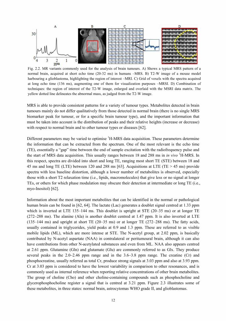
12

MRS is able to provide consistent patterns for a variety of tumour types. Metabolites detected in brain tumours mainly do not differ qualitatively from those detected in normal brain (there is no single MRS biomarker peak for tumour, or for a specific brain tumour type), and the important information that must be taken into account is the distribution of peaks and their relative heights (increase or decrease) with respect to normal brain and to other tumour types or diseases [62]. Different parameters may be varied to optimise 1H-MRS data acquisition. These parameters determine the information that can be extracted from the spectrum. One of the most relevant is the echo time (TE), essentially a “gap” time between the end of sample excitation with the radiofrequency pulse and the start of MRS data acquisition. This usually ranges between 18 and 288 ms in in vivo 1H-MRS. In this respect, spectra are divided into short and long TE, ranging most short TE (STE) between 18 and 45 ms and long TE (LTE) between 120 and 288 ms [63]. Acquisitions at LTE (TE > 45 ms) provide spectra with less baseline distortion, although a lower number of metabolites is observed, especially those with a short T2 relaxation time (i.e., lipids, macromolecules) that give less or no signal at longer TEs, or others for which phase modulation may obscure their detection at intermediate or long TE (i.e., myo-Inositol) [62]. Information about the most important metabolites that can be identified in the normal or pathological human brain can be found in [62, 64]. The lactate (Lac) generates a doublet signal centred at 1.33 ppm which is inverted at LTE 135–144 ms. This doublet is upright at STE (20–35 ms) or at longer TE (272–288 ms). The alanine (Ala) is another doublet centred at 1.47 ppm. It is also inverted at LTE (135–144 ms) and upright at short TE (20–35 ms) or at longer TE (272–288 ms). The fatty acids, usually contained in triglycerides, yield peaks at 0.9 and 1.3 ppm. These are referred to as visible mobile lipids (ML), which are more intense at STE. The N-acetyl group, at 2.02 ppm, is basically contributed by N-acetyl aspartate (NAA) in contralateral or peritumoural brain, although it can also have contributions from other N-acetylated substances and even from ML. NAA also appears centred at 2.61 ppm. Glutamine (Gln) and glutamate (Glu) are commonly referred to as Glx. They produce several peaks in the 2.0–2.46 ppm range and in the 3.6–3.8 ppm range. The creatine (Cr) and phosphocreatine, usually referred as total Cr, produce strong signals at 3.03 ppm and also at 3.93 ppm. Cr at 3.03 ppm is considered to have the lowest variability in comparison to other resonances, and is commonly used as internal reference when reporting relative concentrations of other brain metabolites. The group of choline (Cho) and other choline-containing compounds such as phosphocholine and glycerophosphocholine register a signal that is centred at 3.21 ppm. Figure 2.3 illustrates some of these metabolites, in three states: normal brain, astrocytomas WHO grade II, and glioblastomas.

Fig. 2.2. MR variants commonly used for the analysis of brain tumours. A) Shows a typical MRS pattern of a normal brain, acquired at short echo time (20-32 ms) in humans –MRS. B) T2-W image of a mouse model harbouring a glioblastoma, highlighting the region of interest –MRI. C) Grid of voxels with the spectra acquired at long echo time (136 ms), augmenting one of them for visualization purposes –MRSI. D) Combination of techniques: the region of interest of the T2-W image, enlarged and overlaid with the MSRI data matrix. The yellow dotted line delineates the abnormal mass, as judged from the T2-W image.

13

The rich information contained in MR signals makes them ideally suited to the application of PR techniques [65, 66]. Over the last two decades, these techniques have been successfully applied to the problem of knowledge extraction from human brain tumour data and for diagnosis and prognosis of different pathologies, mostly using single-voxel proton MRS (SV 1H-MRS) [10, 17, 16, 25, 26, 67]. MRSI has been successfully applied to monitoring the metabolic heterogeneity of human brain tumours [39, 45, 46, 68, 69], even at high fields [70]. With regard to animal studies, MRSI has been described mostly for rats [71], especially in brain tumour cases [72, 73, 74]. Nevertheless, improvements in hardware (stronger gradient coils and efficient water cooling systems) and new shimming methods, have enabled MRSI to be performed also in the mouse brain [75, 76].

2.2. Pattern recognition techniques

2.2.1. Supervised methods for the development of MRS data classifiers

In this section, we briefly introduce key concepts for the supervised analysis of MRS data using PR techniques. In general, this analysis involves three main stages: 1) the dimensionality reduction of the data set, i.e. finding a smaller subset (from which the less relevant data features are removed) that still represents the data adequately, with minimum information loss; 2) the classification, i.e. the separation

Fig. 2.3. Important metabolites that can be identified in normal and pathological human brain, at both long (left column, 135-136 ms) and short (right column, 20-32 ms) TE. Top row: UL2 normalised spectra (mean from 15 cases at LTE, and 22 at STE) from normal volunteers. Choline-containing compounds (Cho), creatine and phosphocreatine (Cr) and N-acetyl aspartate (NAA) peaks are pointed out. Middle row: UL2 normalised spectra (mean from 20 cases at LTE, and 22 at STE) from astrocytoma WHO grade II cases. Note the relative increase in the Cho peak, the decrease in both the Cr and NAA, and the appearance of the lactate/mobile lipids (Lac/ML) doublet (mostly lactate) centred at 1.33 ppm (inverted at LTE), as compared to normal brain. Bottom row: UL2 normalised spectra (mean from 79 cases at LTE, and 86 at STE) from glioblastoma cases. Note the relative decrease in the Cho, Cr, and NAA peaks in this malignant tumour type, as well as the increase in Lac/ML (mostly ML), as compared to astrocytomas WHO grade II.

14

of the available data in different classes or categories; and 3) the estimation of the accuracy of this classification/separation.

2.2.1.1. Dimensionality reduction

MRS dataset are frequently scarce and of very high dimensionality, that is, they often consist of a small number of cases and a large number of features. This makes their computer-based automated classification a non-trivial undertaking. Most importantly, this high dimensionality also precludes the straightforward interpretation of the obtained results, limiting their usability in a practical medical context, in which interpretability is paramount and simplicity and robustness of the methods employed are compulsory requirements [77]. The reduction of the dimensionality of a dataset can be seen as a process of selection and/or extraction of relevant features. By removing most irrelevant and redundant information from the data, the valuable selected features help to improve the performance of learning models [78, 79]. Feature selection (FS) and feature extraction (FE) are often performed in MRS datasets prior to diagnostic classification [27, 24]. Selecting the type of FE and FS method is problem and domain dependent, and thus requires knowledge of the domain. Here we outline two of them: PCA and a greedy stepwise approach for FS. PCA is the FE technique most commonly used in MRS data analysis. Standard linear principal components are obtained from the eigenvectors of the covariance matrix –using an orthogonal transformation to convert a set of observations of possibly correlated variables into a set of values of linearly uncorrelated variables called principal components–, and give directions in which the data have maximal variance [79]. That is, for the observed data matrix 𝑉 (𝑑 × 𝑛, where 𝑑 is the data dimensionality and 𝑛 is the number of samples), to find some orthogonal matrix 𝑃 (which rows are the principal components) where 𝑌 = 𝑃𝑉 such that the covariance matrix of 𝑌 ( 1

𝑛−1𝑌𝑌𝑇) is diagonalized.

The columns in 𝑌, then, are the projections onto the basis of the rows in 𝑃. One of the most popular form of feature selection is stepwise sequential, either forward or backward. It is a greedy algorithm that adds the best feature (forward selection, SFS) or deletes the worst feature (backward selection, SBS) at each round. SFS involves starting with no variables in the model, trying out the variables one by one and including them if they are statistically significant. SBS involves starting with all candidate variables and testing them one by one for statistical significance, deleting any that are not significant. In [80], the selection criteria proposed is based on a correlation-based heuristic to evaluate the worth or merit of features, called Correlation-based Feature Subset (CFS) evaluator. It evaluates and hence ranks feature subsets rather than individual features. Regardless of whether a learning system attempts to identify relevant information from a dataset or ignores the issue, reducing the dimensionality can be beneficial, not only to reduce the size of the space and allow algorithms to operate faster and more effectively, but also, at least potentially, to improve the accuracy of the posterior classification. When the dimension of the data is much larger than the number or samples, the models tend to be over-complex, risking data overfitting.

2.2.1.2. Classification

The classification of a sample or pattern may be approached as: 1) a supervised classification (e.g., in Linear Discriminant Analysis, LDA), in which the classes are defined by the system designer, and the input pattern is identified as a member of one of these predefined classes; or 2) an unsupervised

15

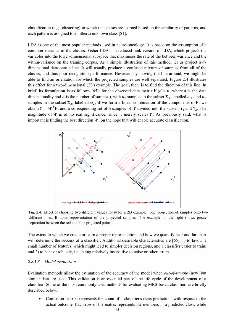
classification (e.g., clustering) in which the classes are learned based on the similarity of patterns, and each pattern is assigned to a hitherto unknown class [81]. LDA is one of the most popular methods used in neuro-oncology. It is based on the assumption of a common variance of the classes. Fisher LDA is a reduced-rank version of LDA, which projects the variables into the lower-dimensional subspace that maximises the rate of the between-variance and the within-variance on the training corpus. As a simple illustration of this method, let us project a 𝑑-dimensional data onto a line. It will usually produce a confused mixture of samples from all of the classes, and thus poor recognition performance. However, by moving the line around, we might be able to find an orientation for which the projected samples are well separated. Figure 2.4 illustrates this effect for a two-dimensional (2D) example. The goal, then, is to find the direction of this line. In brief, its formulation is as follows [65]: for the observed data matrix 𝑉 (𝑑 × 𝑛, where 𝑑 is the data dimensionality and 𝑛 is the number of samples), with 𝑛1 samples in the subset 𝒟1, labelled 𝜔1, and 𝑛2 samples in the subset 𝒟2, labelled 𝜔2; if we form a linear combination of the components of 𝑉, we obtain 𝑌 = 𝑊𝑇𝑉, and a corresponding set of 𝑛 samples of 𝑌 divided into the subsets Υ1 and Υ2. The magnitude of 𝑊 is of no real significance, since it merely scales 𝑌 . As previously said, what is important is finding the best direction 𝑊, on the hope that will enable accurate classification.

The extent to which we create or learn a proper representation and how we quantify near and far apart will determine the success of a classifier. Additional desirable characteristics are [65]: 1) to favour a small number of features, which might lead to simpler decision regions, and a classifier easier to train; and 2) to behave robustly, i.e., being relatively insensitive to noise or other errors.

2.2.1.3. Model evaluation

Evaluation methods allow the estimation of the accuracy of the model when out-of-sample (new) but similar data are used. This validation is an essential part of the life cycle of the development of a classifier. Some of the most commonly used methods for evaluating MRS-based classifiers are briefly described below:

Confusion matrix: represents the count of a classifier's class predictions with respect to the actual outcome. Each row of the matrix represents the members in a predicted class, while

Fig. 2.4. Effect of choosing two different values for 𝑤 for a 2D example. Top: projection of samples onto two different lines. Bottom: representation of the projected samples. The example on the right shows greater separation between the red and blue projected points.

16

each column represents the actual value of members in the original class. It leads naturally to the concepts of sensitivity and specificity described below.

Cross-validation: one round of cross-validation involves partitioning a dataset into complementary subsets, performing the training on one subset, and validating the model on the other. In 𝑘-fold cross-validation, the original dataset is partitioned into 𝑘 subsamples. Of the 𝑘 subsamples, a single subsample is retained for testing the model, and the remaining 𝑘 − 1 subsamples are used as training data. The cross-validation process is then repeated 𝑘 times (the folds), with each of the 𝑘 subsamples used exactly once as testing data. The 𝑘 results from the folds can then be averaged to produce a single estimation of prediction accuracy [65].

Leave-One-Out (LOO): is a special and extreme case of a 𝑘-fold cross-validation. It uses a single case from the original dataset for testing, and the remaining cases are used for training the model. This is repeated so that each case in the dataset is used once as test data. This is the same as a 𝑘-fold cross-validation with 𝑘 being equal to the number of cases in the original dataset.

Bootstrapping: is implemented by constructing a number 𝑛 of bootstrap cases of the observed dataset (and of equal size to the training dataset), each of which is obtained by random sampling with replacement from the original dataset (there is nearly always duplication of individual cases in a bootstrap dataset). The 𝑛 results from the bootstrap samples can then be averaged to produce a single estimation [65]. Bootstrapping could be better at estimating error rates in a linear discriminant problem, outperforming simple cross-validation [82].

Receiver Operating Characteristic (ROC) curve: is a graphical plot of the sensitivity (True Positive Rate, TPR) vs. 1-specificity (False Positive Rate, FPR) for a binary classifier system as its discrimination threshold is varied [83]. It is complemented numerically with the Area Under the Curve (AUC), whose estimation can be interpreted as the probability that the classifier will assign a higher score to a randomly chosen positive sample than to a randomly chosen negative sample.

Balanced Error Rate (BER): is the average of the error rate on the classes, i.e. the average of the proportion of wrong classifications in each class. It is a relevant figure of merit for problems in which classes are unbalanced (a common feature of the data used in this thesis).

Independent test set: there is consensus in the literature that the use of a fully independent test set to validate the "correctness" of a model is one of the most robust evaluation strategies (provided new cases are available), and, to some extent, complementary to the methods described above. It assesses whether a model derived from an analysis of the original data set is transportable to similar cases in another location, providing an insight into the generalisation ability and validity of the model [84]. This strategy involves the comparison of predictions with observations, to obtain accuracy values of the model.

2.2.2. Unsupervised methods for the spectral decomposition of MRS data

ICA and NMF can be seen as DR techniques, functionally similar to source extraction. This section summarily describes some of the existing ICA and NMF methods, used in this thesis for the spectral decomposition of MRS data.

17

2.2.2.1. Independent Component Analysis

This method defines a generative model for the observed multivariate data. In the model, the data variables are assumed to be linear mixtures of some unknown latent variables, and the mixing system is also unknown. The latent variables are assumed non-Gaussian and mutually independent, and they are called the independent components of the observed data [35, 85]. Thus, from an observed data matrix 𝑉 (𝑑 × 𝑛, where 𝑑 is the data dimensionality and 𝑛 is the number of observations), factors 𝑊 (of dimensions 𝑑 × 𝑘 , is the matrix of sources, latent variables, or independent components, where 𝑘 is the number of components) and 𝐻 (of dimensions 𝑘 × 𝑛, is the unknown mixing matrix) can be estimated using ICA, such that 𝑉 ≈ 𝑊𝐻. Two well-known algorithms for the implementation of ICA are considered in this thesis: JADE [86] and FastICA [87]. The former is based on the joint approximative diagonalisation of eigenmatrices, and assumes that the probability density functions of the sources are symmetrical and sufficiently close to normality to be well approximated by an Edgeworth expansion truncated after the fourth-order cumulant. The latter is based on a fixed-point iteration scheme that maximises non-Gaussianity (by the maximisation of the data negentropy) as a measure of statistical independence.

2.2.2.2. Non-negative Matrix Factorisation methods

In NMF methods [36, 48], the data matrix 𝑉 (of dimensions 𝑑 × 𝑛, where 𝑑 is the data dimensionality and 𝑛 is the number of observations), is approximately factorised into two non-negative matrices, the matrix of sources or data basis 𝑊(of dimensions 𝑑 × 𝑘, where 𝑘 is the number of sources, and 𝑘 < 𝑑) and the mixing matrix 𝐻 (of dimensions 𝑘 × 𝑛, each of whose columns provides the encoding of a data point: the spectrum of a voxel in this study). The product of these two matrices provides a good approximation to the original data matrix, in the form:

𝑉 ≈ 𝑊𝐻 (2.1) In this study, the following NMF methods, which cover a wide palette of algorithmic alternatives, were considered:

Euclidean distance update algorithm (herein referred to as euc) [48]. The objective function is optimised with multiplicative update rules for 𝑊 and 𝐻:

𝑊 ← 𝑊 𝑉𝐻𝑇

𝑊𝐻𝐻𝑇 ; 𝐻 ← 𝐻 𝑊𝑇𝑉

𝑊𝑇𝑊𝐻

Monotonic convergence of the algorithm can be proven [48]. These update equations preserve the nonnegativity of 𝑊 and 𝐻, and constrain the columns of 𝑊 to sum to unity.

Alternating least squares (als) [36]. This technique alternately fixes one matrix and improves the other. 𝑊 ← arg min𝑊≥0 𝑓(𝑊, 𝐻); 𝐻 ← arg min𝐻≥0 𝑓(𝑊, 𝐻) where 𝑊 and 𝐻 are updated as follows: 𝑊 ← ((𝐻𝐻𝑇)−1𝐻𝑉𝑇)𝑇; 𝐻 ← (𝑊𝑇𝑊)−1𝑊𝑇𝑉 setting all negative elements in 𝑊 and 𝐻 to zero.

Alternating non-negative least squares using projected gradients (alspg) [88]. The equations for 𝑊 and 𝐻 in the alternating least squares method above are solved here using projected gradients. For 𝐻 this entails:

18

𝐻 ← 𝑃[𝐻 − 𝛼∇𝑓(̅𝐻)] ; where 𝛼 is the step size; and 𝑃[·] is a bounding function that ensures that the solution remains within the boundaries of feasibility. The gradient function is solved as ∇𝑓(̅𝐻) = 𝑊𝑇(𝑊𝐻 − 𝑉). The same approach is used to calculate 𝑊.

Alternating least squares with Optimal Brain Surgeon (OBS) [89] (alsobs) [90]. Similar to alternating least squares, this algorithm alternately solves the least squares equations for 𝑊 and 𝐻. The negative elements in 𝑊 and 𝐻 are set to zero and the rest are adjusted using the OBS method, through second-order derivatives. The update rules for 𝑊 and 𝐻 are: 𝑊 ← ((𝐻𝐻𝑇)−1𝐻𝑉𝑇)𝑇 + 𝛿𝑊, and 𝐻 ← (𝑊𝑇𝑊)−1𝑊𝑇𝑉 + 𝛿𝐻 ; where 𝛿𝑊 and 𝛿𝐻 act as regularisation terms and are responsible for eliminating the less important elements of 𝑊 and 𝐻 , respectively (the original OBS was used as a weight pruning mechanism in artificial neural networks), thus re-adjusting the remaining elements optimally. More implementation details can be found in [91].

Convex-NMF [42]. To achieve interpretability, this method imposes a constraint that the vectors (columns) defining 𝑊 must lie within the column space of 𝑉, i.e. 𝑊 = 𝑉𝐴 (where 𝐴 is an auxiliary adaptative weight matrix that fully determines 𝑊), so that 𝑉 ≈ 𝑉𝐴𝐻. By restricting 𝑊 to convex combinations of the columns of 𝑉 we can, in fact, understand each of the basis or sources as weighted sums of data points. Unlike the previous ones, this NMF variant applies to both nonnegative and mixed-sign data matrices. The factors 𝐻 and 𝐴 are updated as follows:

𝐻𝑇 ← 𝐻𝑇√(𝑉𝑇𝑉)+𝐴 + 𝐻𝑇𝐴𝑇(𝑉𝑇𝑉)−𝐴

(𝑉𝑇𝑉)−𝐴 + 𝐻𝑇𝐴𝑇(𝑉𝑇𝑉)+𝐴 , 𝐴 ← 𝐴√

(𝑉𝑇𝑉)+𝐻𝑇 + (𝑉𝑇𝑉)−𝐴𝐻𝐻𝑇

(𝑉𝑇𝑉)−𝐻𝑇 + (𝑉𝑇𝑉)+𝐴𝐻𝐻𝑇

where (·)+ is the positive part of the matrix, where all negative values become zeros; and (·)− is the negative part of the matrix, where all positive values become zeros.

19

3.

Supervised MRS data classifier-

development system

3.1. Introduction

The need for software tools that allowed a rapid development of multiple classifiers for the already existing databases available [15] fostered the development of SpectraClassifier (SC). This is a free, multiplatform, java language solution for the design and implementation of classifiers based on MRS data. It should also allow to rapidly test hypothesis that may surface during the lengthy process of data collection. MRS data are commonly analysed with either commercial (SPSS [92], SAS [93], SIMCA-P+ [94]), non-commercial (R [95]), or user-written scripts running over proprietary packages such as MATLAB [96], and usually require a certain degree of mathematical expertise for testing each individual hypothesis [24, 25, 26]. Some other packages for PR and classifier development (AMIX [97] and Pirouette [98]) are less complex tools, but commercial. Furthermore, Pirouette is platform-limited, because it is designed specifically for the Windows operating system. SC is intended to facilitate the development of MRS-based classifiers. Its main goal is to allow a user with minimum background knowledge of multivariate statistics to perform a fully automated PR analysis, from the feature extraction and/or selection stage to the evaluation of the developed classifier. The purpose of this chapter is to describe SC, from the algorithms implemented to its main functionalities.

3.2. Materials and methods

3.2.1. Description of the data

The single-voxel proton MRS (SV 1H-MRS) data used for the developments reported in this chapter were extracted from INTERPRET, an international multi-centre database [15], which was the result of the INTERPRET European research project* [13]. Class labelling was performed according to the World Health Organisation (WHO) system for diagnosing brain tumours by histopathological analysis of a biopsy sample. These data are acquired at 1.5T and at two different echo times (short, 20-32 ms (STE) and long, 135-144 ms (LTE)) from brain tumour patients and healthy controls (that is, two spectra, one at STE and another at LTE, are available for each individual). Data were processed as in [14]. A total of 195 clinically-relevant frequency intensity values measured in parts per million (ppm)

* http://gabrmn.uab.es/interpret

20

were sampled from each spectrum in the [4.24,0.50]ppm interval. Unit length normalisation (UL2) of the spectra was performed: the squares of the values in the interval of interest of the data vector were summed and each intensity was divided by the square root of this sum (𝐼𝑛(𝑖) = 𝐼(𝑖) √∑ 𝐼(𝑖)2

𝑎𝑙𝑙 𝑖𝑛𝑡𝑒𝑛𝑠𝑖𝑡𝑖𝑒𝑠⁄ , where 𝐼𝑛 is the unit length normalised intensity for each data point 𝑖, and 𝐼 represents the initial intensity for normalisation). This normalisation method is preferred for spectra which have a number of points with negative intensities [11]. The importance of using two different signal acquisition conditions (STE and LTE) lies in the different metabolites that are detectable at each of them. STE is more sensitive to those with short T2 (an MR relaxation time parameter) values (it is, for example, more adequate to detect mobile lipids, ML) and, in addition, all signal peaks are positive. On the other hand, in LTE spectra we can find both positive and negative peaks, where the negative peak is mostly due to the inverted Alanine (Ala) or Lactate (Lac) doublets. A small subset of the INTERPRET database was used in this chapter to illustrate both the development of classifiers using SC and their validation. This subset included, at STE, 58 low grade meningiomas (MM), 86 glioblastomas (GL), 38 metastases (ME), 22 astrocytomas grade II (A2), 6 oligoastrocytomas (OA), and 7 oligodendrogliomas (OD); at LTE, it included 55 MM, 78 GL, 31 ME, 20 A2, 6 OA, 5 OD.

3.2.2. Feature selection or extraction

Several FS or FE methods based on pattern recognition were applied to the significant part of the spectra (MRS frequencies, in this case), looking for a subset of relevant peak heights of typical resonances (ppm, “part per million”) or a reduced representation set of combinations of them. SC implements two sequential FS methods based on a “hill climbing” search (Greedy Stepwise approach), either forward or backward, and evaluates the selected features with a CFS (Correlation-based Feature Subset) evaluator [80]. This Java class evaluates the worth of a subset of attributes by considering the individual predictive ability of each feature along with the degree of redundancy between them. Subsets of features that are highly correlated with the class while having low intercorrelation are preferred. PCA is the FE method implemented. It performs a principal components analysis and transformation of the data, used in conjunction with a Ranker search (for ranking attributes by their individual evaluations). DR is accomplished by choosing enough eigenvectors to account for a predefined percentage of the variance in the original data (we set it by default to cover a 95% of the variance, but this value can be modified by the user). Attribute noise can be filtered by transforming to the principal component space, eliminating some of the worst eigenvectors, and then transforming back into the original space.

3.2.3. Implementation of the classifier

The purpose of creating a classifier is to separate data cases into one of two or more classes based on a set of features that describe the data in the best manner (features selected and/or extracted). In general, we assign a data case to one of a number of classes based on observations made on the data. These classes are already known or predetermined.

21

At the moment, SC uses Fisher Linear Discriminant Analysis (LDA) as the technique of choice for distinguishing cases between two, three or four classes. Fisher LDA is a fundamental and widely used technique that provides a reasonable way of reducing the dimensionality of the problem [65]. With this software, the user can assign each class to a different tumour type, or to a super-class generated by grouping tumour types [4]. As the original version of Fisher LDA does not assume any probability distribution to define the model, the limitation of Fisher LDA for estimating the probability of a case of belonging to a class, has been overcome by approximating the resulting projections through spherical Gaussian distributions, one for each class. The centre of each distribution has been assumed as the class mean estimated from data and the standard deviation common to all. Therefore, the probability of membership of every case to each class is estimated applying the Bayes’ theorem over these distributions [65].

3.2.4. Evaluation of the classifiers

SC implements some of the most commonly used methods for evaluating MRS-based classifiers: confusion matrix, cross-validation, LOO, bootstrapping, ROC curve and AUC. In SC, the 𝑘 value (the number of partitioned subsamples) of the cross-validation can be set by the user. It is typically used in scenarios where the goal is prediction, and it is desirable to estimate how accurately a predictive model will perform in practice. The 𝑛 value (the number of bootstrap cases of the observed dataset) in the bootstrapping is equal to 1,000 by default, but this value can be modified by the user.

3.3. Results

3.3.1. Classifier design

When SC is launched, Classifier design (figure 3.1) is the first tab that can be seen. This tab allows the user to tune the desired input parameters for designing a classifier, such as the training datasets, the definition of classes and the selection or extraction of relevant features, which will be used as classifier inputs. The development of a well-known three-class classifier using SC is used as illustration throughout this chapter, using STE SV data. Here, “Class 1” is named low-grade m and contains the MM cases; “Class 2” is named aggressive and contains GL and ME; and “Class 3” is named low-grade g and contains A2, OA and OD.

3.3.2. Data exploration

Data exploration is the second tab of the application. It can be used to plot the spectrum of individual cases; to plot the mean and the standard deviation (SD) of a set of cases; as well as to display the features obtained in the FS process (figure 3.2).

22

Fig. 3.2. Data exploration tab. Three of the four visualizers are showing the feature selection results: the mean (pink spectrum), the standard deviation range (yellow line) and the selected features (green vertical lines).

Fig. 3.1. Classifier design tab. It allows data entry, class configuration, FS/FE, and development of the classifier.

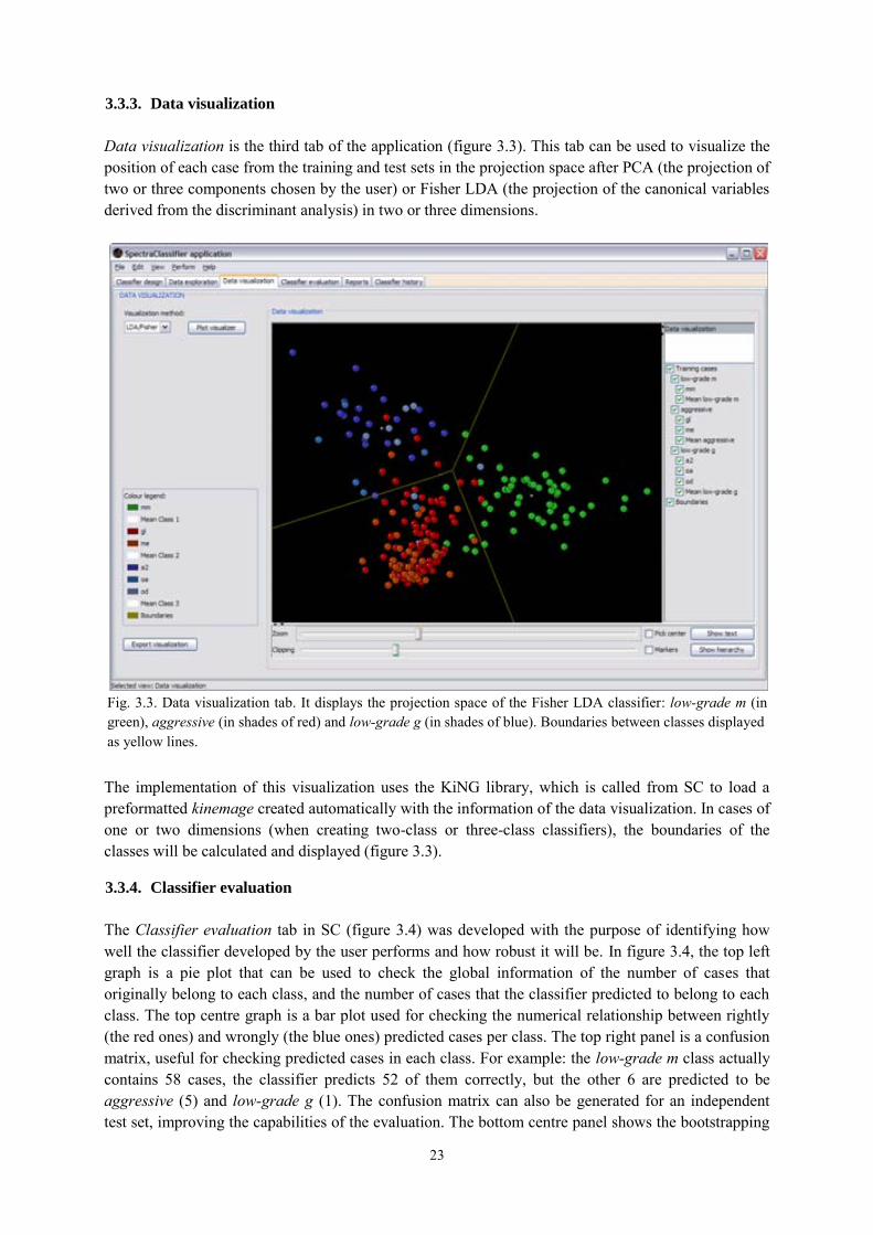
23

3.3.3. Data visualization

Data visualization is the third tab of the application (figure 3.3). This tab can be used to visualize the position of each case from the training and test sets in the projection space after PCA (the projection of two or three components chosen by the user) or Fisher LDA (the projection of the canonical variables derived from the discriminant analysis) in two or three dimensions.

The implementation of this visualization uses the KiNG library, which is called from SC to load a preformatted kinemage created automatically with the information of the data visualization. In cases of one or two dimensions (when creating two-class or three-class classifiers), the boundaries of the classes will be calculated and displayed (figure 3.3).

3.3.4. Classifier evaluation

The Classifier evaluation tab in SC (figure 3.4) was developed with the purpose of identifying how well the classifier developed by the user performs and how robust it will be. In figure 3.4, the top left graph is a pie plot that can be used to check the global information of the number of cases that originally belong to each class, and the number of cases that the classifier predicted to belong to each class. The top centre graph is a bar plot used for checking the numerical relationship between rightly (the red ones) and wrongly (the blue ones) predicted cases per class. The top right panel is a confusion matrix, useful for checking predicted cases in each class. For example: the low-grade m class actually contains 58 cases, the classifier predicts 52 of them correctly, but the other 6 are predicted to be aggressive (5) and low-grade g (1). The confusion matrix can also be generated for an independent test set, improving the capabilities of the evaluation. The bottom centre panel shows the bootstrapping

Fig. 3.3. Data visualization tab. It displays the projection space of the Fisher LDA classifier: low-grade m (in green), aggressive (in shades of red) and low-grade g (in shades of blue). Boundaries between classes displayed as yellow lines.

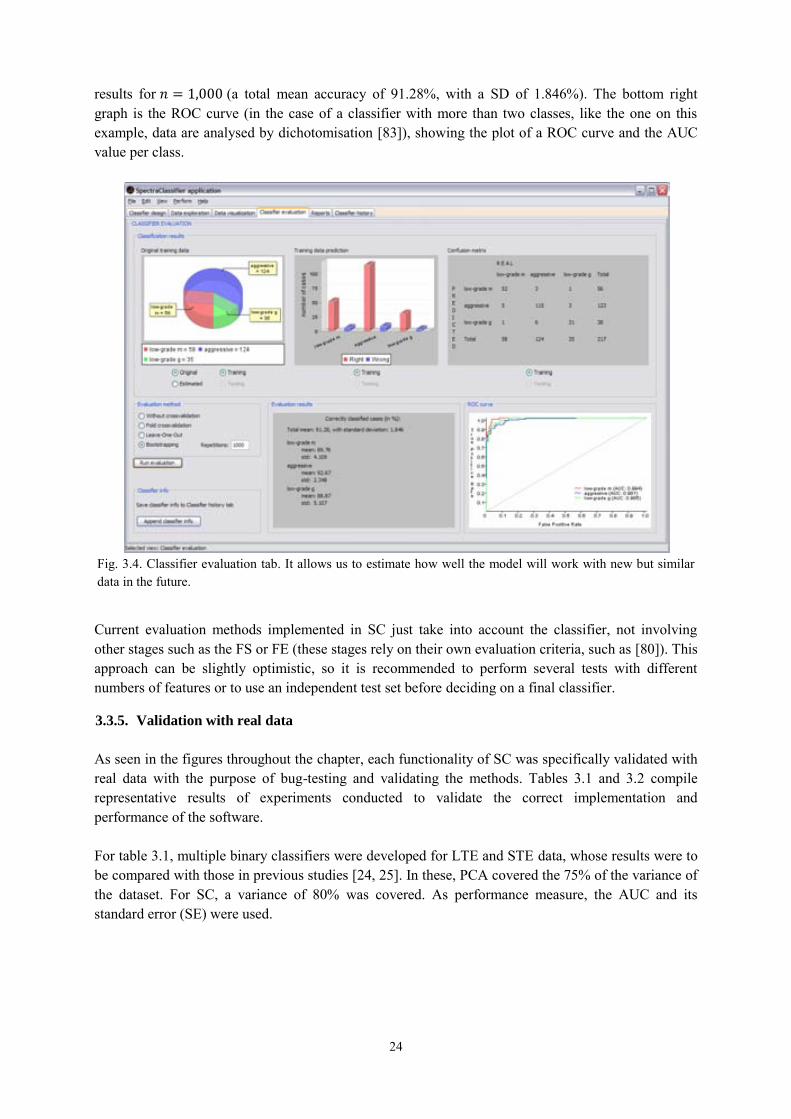
24

results for 𝑛 = 1,000 (a total mean accuracy of 91.28%, with a SD of 1.846%). The bottom right graph is the ROC curve (in the case of a classifier with more than two classes, like the one on this example, data are analysed by dichotomisation [83]), showing the plot of a ROC curve and the AUC value per class.

Current evaluation methods implemented in SC just take into account the classifier, not involving other stages such as the FS or FE (these stages rely on their own evaluation criteria, such as [80]). This approach can be slightly optimistic, so it is recommended to perform several tests with different numbers of features or to use an independent test set before deciding on a final classifier.

3.3.5. Validation with real data

As seen in the figures throughout the chapter, each functionality of SC was specifically validated with real data with the purpose of bug-testing and validating the methods. Tables 3.1 and 3.2 compile representative results of experiments conducted to validate the correct implementation and performance of the software. For table 3.1, multiple binary classifiers were developed for LTE and STE data, whose results were to be compared with those in previous studies [24, 25]. In these, PCA covered the 75% of the variance of the dataset. For SC, a variance of 80% was covered. As performance measure, the AUC and its standard error (SE) were used.

Fig. 3.4. Classifier evaluation tab. It allows us to estimate how well the model will work with new but similar data in the future.

25

The results in table 3.2 correspond to the evaluation of a three-class classifier: low grade meningiomas (MM), aggressive (GL + ME) and low grade glial (A2, OD, OA), at STE, LTE and the combination by concatenation [28] of LTE + STE. In [28], k-Random sampling train-test (kRSTT) with stratified test sets with 150 repetitions was the evaluation procedure used. In SC, a bootstrap method with 1,000 repetitions was used. Although both methods used to evaluate the classifiers are not exactly the same, both are equivalent sampling methods, therefore their results can be directly compared. The accuracy (with SD) was used as a figure of merit for the performance.

In general terms, the results obtained with SC compare well with previous non-automated analyses of the same dataset [13, 24, 25, 26, 27, 28]. Sample brain tumour data from real patients are distributed with SC for testing purposes.

3.3.6. Computation time

The computation time needed to develop a classifier depends on the dataset size. For example, in a 3GHz CPU and 2GB RAM personal computer, the typical performance values for INTERPRET 512 points/frequencies files (188 of them in the range of interest) in a classification problem with 217 cases and three classes are around 4 seconds for FS with the sequential forward method and 3 seconds for Fisher LDA. For the same problem with concatenated spectra (i.e. 1024 points, 376 points in the range of interest, and 195 cases), the corresponding computation times are in the area of 50 and 3 seconds, respectively. For High Resolution Magic Angle Spinning (HR-MAS) spectra of 1639 points (1310 points in the range of interest), FS takes 30 minutes with the same conditions. The computation time should be considerably reduced using a high performance server.

3.4. Discussion

SC is a user-friendly software tool developed for performing PR of MRS data, which was designed to fulfil the real needs of potential users in the MRS community. It works with all types of MRS, i.e. SV, MV and HR-MAS data. In addition, it also supports two concatenated spectra of the same resolution and number of points, since it had been previously shown that combination of data from two different TEs can provide useful additional information for classification [28, 63]. SC allows easy data exploration, with four different spectra visualizers through which individual cases, class mean, SD, as well as the selected classification features in each experiment can be explored.

Accuracy ± SD in [28] Accuracy ± SD in SC STE 88.82 ± 4.51 90.73 ± 1.97 LTE 82.50 ± 5.31 85.12 ± 2.51 LTE + STE 88.71 ± 4.54 90.31 ± 2.16

Table 3.2. Comparison of results for the validation of SC, using FS prior to LDA.

Classes LTE - [24] LTE - SC STE - [25] STE - SC GL vs. MM 0.953 ± 0.031 (8) 0.977 ± 0.016 (8) 0.956 ± 0.028 (4) 0.923 ± 0.028 (4) GL vs. ME 0.593 ± 0.104 (6) 0.757 ± 0.054 (6) 0.591 ± 0.097 (4) 0.688 ± 0.056 (4) GL vs. A2 0.918 ± 0.063 (7) 0.941 ± 0.025 (7) 0.966 ± 0.029 (3) 0.962 ± 0.019 (3) MM vs. ME 0.961 ± 0.038 (5) 0.970 ± 0.028 (5) 0.954 ± 0.044 (4) 0.972 ± 0.021 (4) MM vs. A2 0.931 ± 0.073 (10) 0.999 ± 0.003 (10) 0.997 ± 0.009 (11) 1.000 ± 0.000 (11) ME vs. A2 0.961 ± 0.053 (4) 0.995 ± 0.010 (4) 0.986 ± 0.025 (2) 0.979 ± 0.025 (2)

Table 3.1. Comparing results for the validation of SC, using PCA prior to LDA. The values in the cells correspond to the AUC ± SE. The number in parenthesis indicates the number of principal components used.

26

Classification results are shown both visually and numerically. The data visualization tab allows feedback on classification errors through potential outlier analysis by using the four spectra visualizers. The software in its current instantiation is limited to a small number of PR techniques, corresponding to the most commonly used in the area. Other widely used software tools [21, 22, 23], such as SIMCA-P+, AMIX, and Pirouette, offering methods such as PCA, Partial Least Square (PLS), Soft Independent Modelling of Class Analogy (SIMCA), Principal Component Regression (PCR), and Classical Least Square (CLS), also have this limitation.

3.4.1. Applying SpectraClassifier in further studies

This section presents two published studies that benefitted from the use of SC in terms of data analysis, accuracy of the results obtained, and computation time saved.

3.4.1.1. Choosing optimal classifiers for pseudotumoural brain diseases in humans

The purpose of this study [29] was to choose optimum classifiers for differentiating between tumoural disease, pseudotumoural disease and normal brain with SV 1H-MRS at STE and LTE, with the help of a test set to validate the results. The dataset analysed was gathered from patients explored at IDI-Bellvitge (Barcelona, Spain) and divided into training and test set. The inclusion criteria were: 1) presence of an untreated solid, non-necrotic brain mass suggesting a brain tumour, 2) diagnosis of pseudotumoural disease or glial tumour grades WHO II or III, 3) spectra available at both STE and LTE, and 4) spectra to be of good quality. Five normal volunteers were selected from retrospective cases acquired at the same institution. The dataset for training included 46 tumours, 19 pseudotumours, and 5 normal brain patients; and the test set included 12 tumours, and 7 pseudotumours. Figure 3.5 presents some of the obtained results, showing the accuracy of each classifier. Criteria for choosing the best classifier at each TE were, in this order: best behaviour with the test set, best accuracy after the bootstrapping and the minimum necessary number of features.

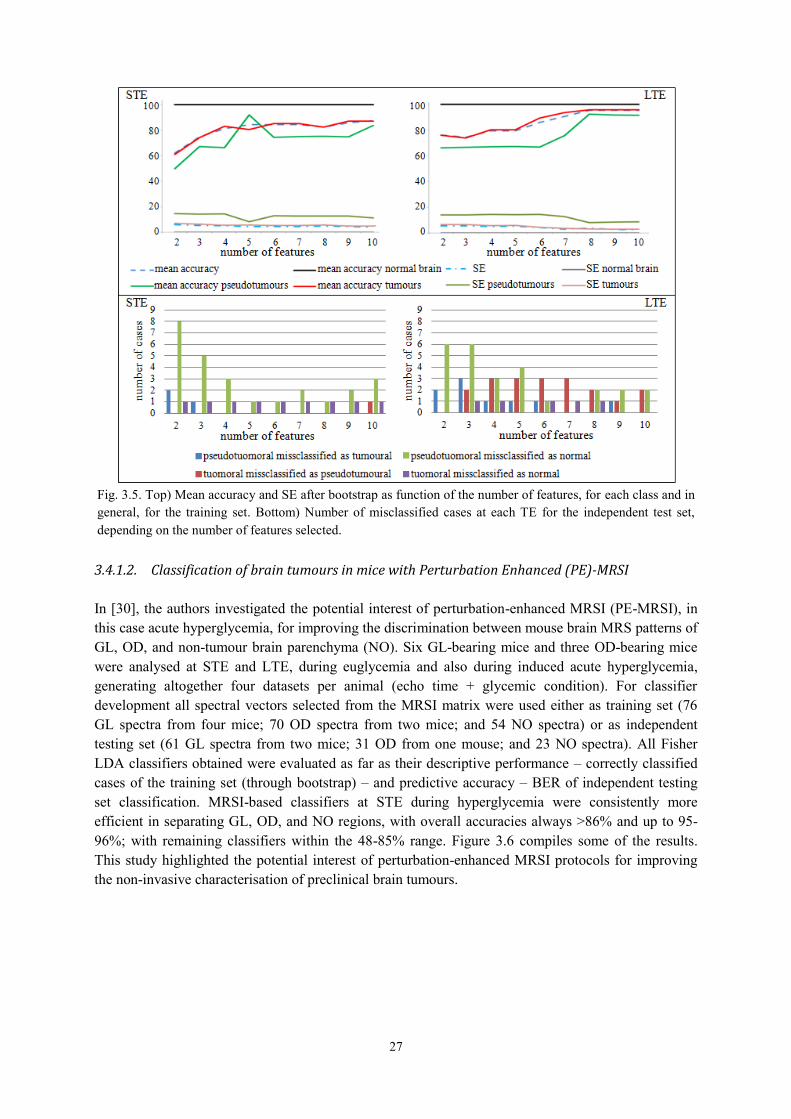
27

3.4.1.2. Classification of brain tumours in mice with Perturbation Enhanced (PE)-MRSI

In [30], the authors investigated the potential interest of perturbation-enhanced MRSI (PE-MRSI), in this case acute hyperglycemia, for improving the discrimination between mouse brain MRS patterns of GL, OD, and non-tumour brain parenchyma (NO). Six GL-bearing mice and three OD-bearing mice were analysed at STE and LTE, during euglycemia and also during induced acute hyperglycemia, generating altogether four datasets per animal (echo time + glycemic condition). For classifier development all spectral vectors selected from the MRSI matrix were used either as training set (76 GL spectra from four mice; 70 OD spectra from two mice; and 54 NO spectra) or as independent testing set (61 GL spectra from two mice; 31 OD from one mouse; and 23 NO spectra). All Fisher LDA classifiers obtained were evaluated as far as their descriptive performance – correctly classified cases of the training set (through bootstrap) – and predictive accuracy – BER of independent testing set classification. MRSI-based classifiers at STE during hyperglycemia were consistently more efficient in separating GL, OD, and NO regions, with overall accuracies always >86% and up to 95-96%; with remaining classifiers within the 48-85% range. Figure 3.6 compiles some of the results. This study highlighted the potential interest of perturbation-enhanced MRSI protocols for improving the non-invasive characterisation of preclinical brain tumours.

Fig. 3.5. Top) Mean accuracy and SE after bootstrap as function of the number of features, for each class and in general, for the training set. Bottom) Number of misclassified cases at each TE for the independent test set, depending on the number of features selected.

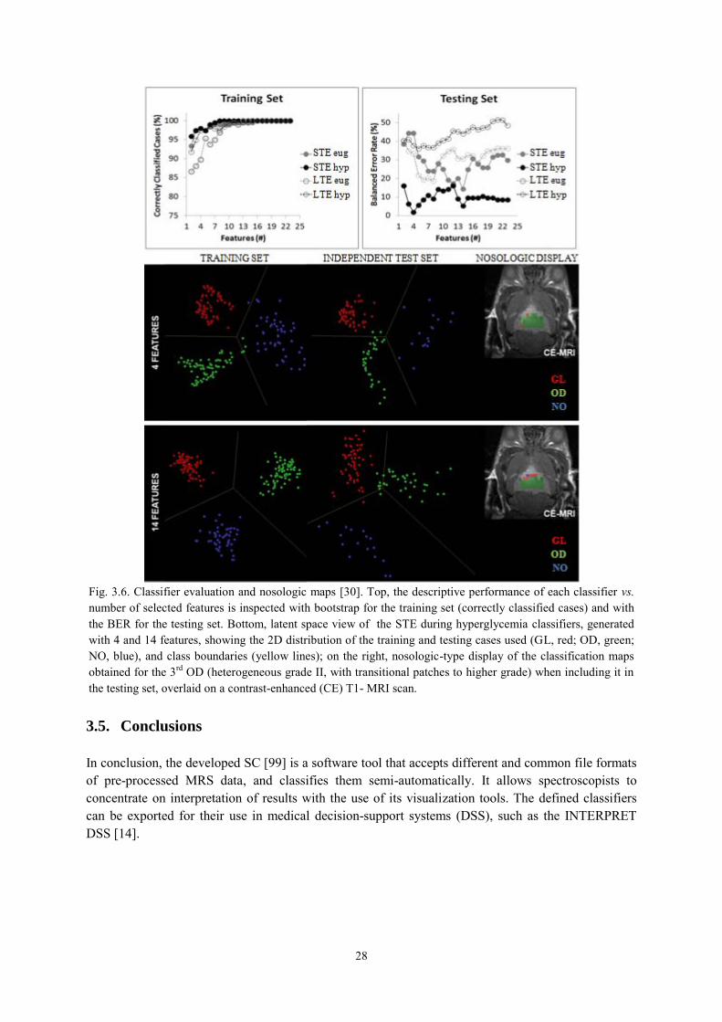
28

3.5. Conclusions

In conclusion, the developed SC [99] is a software tool that accepts different and common file formats of pre-processed MRS data, and classifies them semi-automatically. It allows spectroscopists to concentrate on interpretation of results with the use of its visualization tools. The defined classifiers can be exported for their use in medical decision-support systems (DSS), such as the INTERPRET DSS [14].

Fig. 3.6. Classifier evaluation and nosologic maps [30]. Top, the descriptive performance of each classifier vs. number of selected features is inspected with bootstrap for the training set (correctly classified cases) and with the BER for the testing set. Bottom, latent space view of the STE during hyperglycemia classifiers, generated with 4 and 14 features, showing the 2D distribution of the training and testing cases used (GL, red; OD, green; NO, blue), and class boundaries (yellow lines); on the right, nosologic-type display of the classification maps obtained for the 3rd OD (heterogeneous grade II, with transitional patches to higher grade) when including it in the testing set, overlaid on a contrast-enhanced (CE) T1- MRI scan.

29

4.

Spectral Prototype Extraction for

dimensionality reduction

4.1. Introduction

FS and FE for DR are often performed in MRS datasets prior to diagnostic classification [24, 27]. PCA is, by far, the FE technique most commonly used in MRS data analysis. Unfortunately, PCA has some important limitations in this scenario: First, the DR results are bound to be affected by the presence of uniformative noise in the data, which is commonplace in MRS. Secondly, the resulting components must be selected according to some ad hoc thresholding on the basis of variance retention. Thirdly, each component is a linear combination of all the spectral frequencies; this seriously limits the interpretability of the results, which is paramount in brain tumour diagnosis. Finally, PCA (and, by that matter, other FE techniques used for the same purpose, such as ICA, completely bypasses the fact that MRS data do not comply with the independent and identically-distributed (i.i.d.) condition. In this brief chapter, we define a novel FE technique, namely Spectral Prototype Extraction (SPE), that overcomes the aforementioned limitations of PCA and similar techniques. It is based on a manifold-constrained Hidden Markov Model (HMM), suitable for non-i.i.d. data, and its formulation within a variational Bayesian framework imbues it with regularisation properties that minimise the negative effect of the presence of noise in the data. This model, Variational Bayesian Generative Topographic Mapping Through Time (VB-GTM-TT, [34]) segments the MRS in an interpretable way. Its use for FE in MRS is illustrated here in a difficult brain tumour classification problem: that of discriminating between glioblastomas and metastases, two types of aggressive brain tumours.



The analysed data were extracted from the INTERPRET database [15], as described in chapter 3. Here, the subset considered included: a total of 124 cases at STE, that is 86 GL and 38 ME; a total of 109 at LTE, including 78 GL and 31 ME; and 109 items built by combination (through concatenation) [28] of the spectra measured at LTE and STE for the same patients. These frequencies become the data features in all cases.

4.2.2. Spectral Prototype Extraction using VB-GTM-TT

Manifold learning techniques are meant to model usually complex and high-dimensional multivariate data through simpler low-dimensional, manifold-based representations. When defined within the

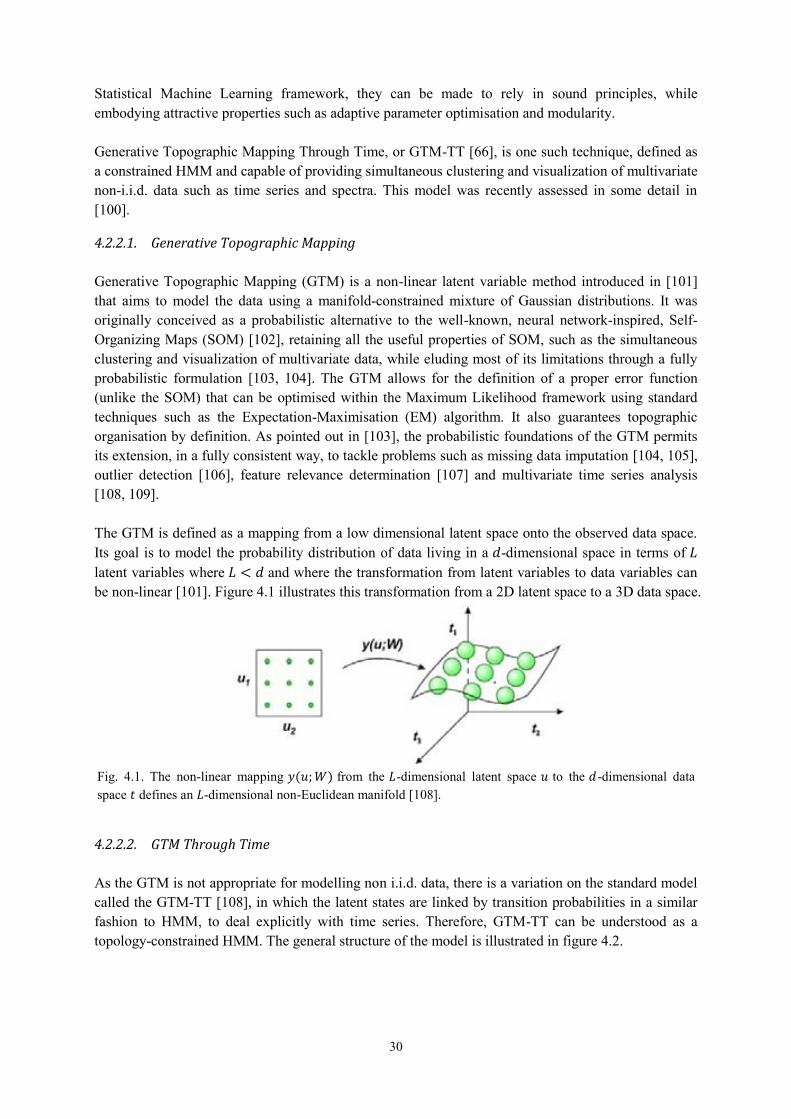
30

Statistical Machine Learning framework, they can be made to rely in sound principles, while embodying attractive properties such as adaptive parameter optimisation and modularity. Generative Topographic Mapping Through Time, or GTM-TT [66], is one such technique, defined as a constrained HMM and capable of providing simultaneous clustering and visualization of multivariate non-i.i.d. data such as time series and spectra. This model was recently assessed in some detail in [100].

4.2.2.1. Generative Topographic Mapping

Generative Topographic Mapping (GTM) is a non-linear latent variable method introduced in [101] that aims to model the data using a manifold-constrained mixture of Gaussian distributions. It was originally conceived as a probabilistic alternative to the well-known, neural network-inspired, Self-Organizing Maps (SOM) [102], retaining all the useful properties of SOM, such as the simultaneous clustering and visualization of multivariate data, while eluding most of its limitations through a fully probabilistic formulation [103, 104]. The GTM allows for the definition of a proper error function (unlike the SOM) that can be optimised within the Maximum Likelihood framework using standard techniques such as the Expectation-Maximisation (EM) algorithm. It also guarantees topographic organisation by definition. As pointed out in [103], the probabilistic foundations of the GTM permits its extension, in a fully consistent way, to tackle problems such as missing data imputation [104, 105], outlier detection [106], feature relevance determination [107] and multivariate time series analysis [108, 109]. The GTM is defined as a mapping from a low dimensional latent space onto the observed data space. Its goal is to model the probability distribution of data living in a 𝑑-dimensional space in terms of 𝐿 latent variables where 𝐿 < 𝑑 and where the transformation from latent variables to data variables can be non-linear [101]. Figure 4.1 illustrates this transformation from a 2D latent space to a 3D data space.

4.2.2.2. GTM Through Time

As the GTM is not appropriate for modelling non i.i.d. data, there is a variation on the standard model called the GTM-TT [108], in which the latent states are linked by transition probabilities in a similar fashion to HMM, to deal explicitly with time series. Therefore, GTM-TT can be understood as a topology-constrained HMM. The general structure of the model is illustrated in figure 4.2.

Fig. 4.1. The non-linear mapping 𝑦(𝑢; 𝑊) from the 𝐿-dimensional latent space 𝑢 to the 𝑑-dimensional data space 𝑡 defines an 𝐿-dimensional non-Euclidean manifold [108].

31

4.2.2.3. Variational Bayesian GTM-TT

The presence of uninformative noise in a dataset and the associated potential problem of data overfitting can seriously hamper the modelling of non-i.i.d. data. In its basic formulation, GTM-TT is prone to overfitting unless active regularisation methods are applied. The reformulation of this model within a fully Bayesian framework using variational approximations confers it with regularisation capabilities in a natural way. The resulting VB-GTM-TT has been shown to be robust, and to deal effectively with the problem of overfitting [34]. Variational inference allows the definition of a lower bound for the marginal log-likelihood of the model, defined as:

ln 𝑝(𝑋) = ln ∫ ∑ 𝑝(𝑍, 𝑋|𝛩)𝑝(𝛩)

all 𝑍

𝑑𝛩

where 𝑋 are the MRS data; 𝑍 are the hidden states defined by the model; and 𝛩 are the model parameters, including a matrix with the centroids or prototypes embedded in the model manifold 𝑌, initial state probabilities 𝜋, and transition probabilities 𝐴. These parameters depend, in turn, on a set of hyperparameters 𝜈, 𝜆, 휀, 𝛼, 𝑑𝛽 , 𝑠𝛽 . The complete model is graphically illustrated by figure 4.3. Details on parameter estimation and the calculations involved can be found elsewhere [34].

4.2.2.4. Spectral Prototype Extraction

Fig. 4.3. Graphical representation of the Bayesian GTM-TT model. Variables are noted by circles, parameters, by squares, and hyperparameters, by rounded squares.

Fig. 4.2. The temporal version of GTM consists of a HMM in which the hidden states are given by the latent points of the GTM model, and the emission probabilities are governed by the GTM mixture distribution [108].

32

The VB-GTM-TT provides a hidden space representation of the data by assigning each point (in the case of MRS data, each spectral frequency) to the hidden state bearing maximum responsibility for the generation of that point. Hidden states are arranged in a regular and topology-preserving 2-D grid for data visualization. This mapping assignment (equivalent to a cluster-membership assignment) is carried out according to a mode-projection that takes the form ℎℎ

𝑚𝑜𝑑𝑒 = 𝑎𝑟𝑔𝑚𝑎𝑥𝑘⟨𝑧𝑘,𝑛⟩ , where the variational parameter 𝑧𝑘,𝑛 is calculated as part of the model estimation of its adaptive parameters and represents the probability for each hidden state of being the generator of each data point. Each spectral frequency is therefore assigned to what we call here a spectral prototype (SP). Importantly, previous research [34] has shown that VB-GTM-TT, unlike unregularised counterparts, models data using a very limited number of non-empty hidden states (SPs). This behaviour eliminates the need to select a number of extracted features. Another consequence of this assignment procedure is that each of the MRS frequencies will be assigned solely to one SP. Moreover, given the HMM-based nature of the model, each SP is likely to consist of complete intervals of frequencies or collections of these intervals. All these should make the interpretation of the SPE process easier than PCA and similar methods. Figure 4.4 illustrates how the method works.

Fig. 4.4. Graphical representation of the SPE stages. The stages are represented with numbered red squares. The black arrows symbolise the transition from each stage to the next one. Stage 1) shows the original set of MRS cases. Each spectral frequency (in ppm) corresponds to an attribute (att), in order of appearance. Stage 2) illustrates how the dataset is built: each column corresponds to the spectrum of one of the cases, and the rows contain the attributes. Stage 3) shows the representation of this dataset in the GTM-TT model. Attribute 1 (att1) is a vector represented with a point in the high dimensional data space (three dimensions here, for visualization purposes), that is assumed to be generated by a point in the latent space (in red). Stage 4) groups all the information, illustrating the 2D latent space (the hidden states are arranged in a regular and topology-preserving 2D grid for data visualization), and the high-dimensional data space of all attributes. Stage 5) shows a representation of a set of basis functions arranged on a regular grid and defined in the original GTM as spherical symmetric Gaussians. The mapping assignment (red arrows) represents the probability for each hidden state of being the generator of each data point. Each spectral frequency is therefore assigned to what we call here a SP. Stage 6) illustrates the representation of the SP (A and B in the example), each of which is likely to consist of intervals of frequencies or collections of these intervals.

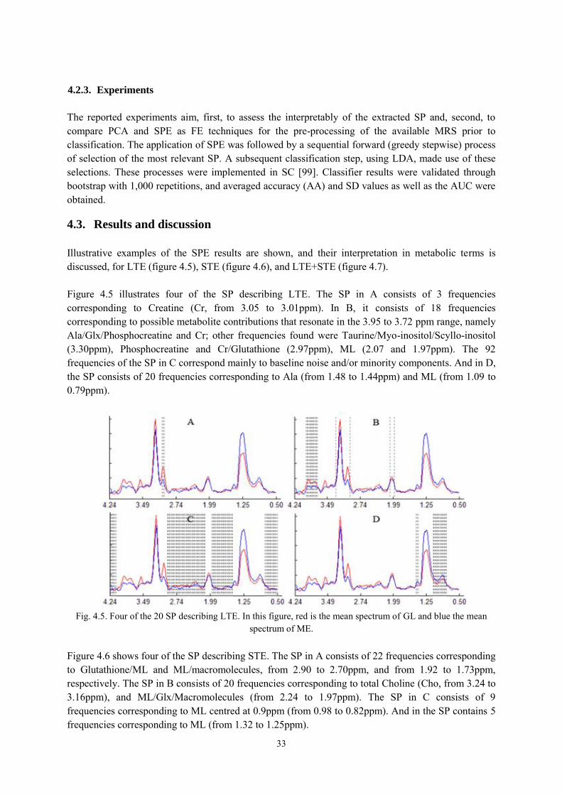
33

4.2.3. Experiments

The reported experiments aim, first, to assess the interpretably of the extracted SP and, second, to compare PCA and SPE as FE techniques for the pre-processing of the available MRS prior to classification. The application of SPE was followed by a sequential forward (greedy stepwise) process of selection of the most relevant SP. A subsequent classification step, using LDA, made use of these selections. These processes were implemented in SC [99]. Classifier results were validated through bootstrap with 1,000 repetitions, and averaged accuracy (AA) and SD values as well as the AUC were obtained.

4.3. Results and discussion

Illustrative examples of the SPE results are shown, and their interpretation in metabolic terms is discussed, for LTE (figure 4.5), STE (figure 4.6), and LTE+STE (figure 4.7). Figure 4.5 illustrates four of the SP describing LTE. The SP in A consists of 3 frequencies corresponding to Creatine (Cr, from 3.05 to 3.01ppm). In B, it consists of 18 frequencies corresponding to possible metabolite contributions that resonate in the 3.95 to 3.72 ppm range, namely Ala/Glx/Phosphocreatine and Cr; other frequencies found were Taurine/Myo-inositol/Scyllo-inositol (3.30ppm), Phosphocreatine and Cr/Glutathione (2.97ppm), ML (2.07 and 1.97ppm). The 92 frequencies of the SP in C correspond mainly to baseline noise and/or minority components. And in D, the SP consists of 20 frequencies corresponding to Ala (from 1.48 to 1.44ppm) and ML (from 1.09 to 0.79ppm).

Figure 4.6 shows four of the SP describing STE. The SP in A consists of 22 frequencies corresponding to Glutathione/ML and ML/macromolecules, from 2.90 to 2.70ppm, and from 1.92 to 1.73ppm, respectively. The SP in B consists of 20 frequencies corresponding to total Choline (Cho, from 3.24 to 3.16ppm), and ML/Glx/Macromolecules (from 2.24 to 1.97ppm). The SP in C consists of 9 frequencies corresponding to ML centred at 0.9ppm (from 0.98 to 0.82ppm). And in the SP contains 5 frequencies corresponding to ML (from 1.32 to 1.25ppm).

Fig. 4.5. Four of the 20 SP describing LTE. In this figure, red is the mean spectrum of GL and blue the mean

spectrum of ME.

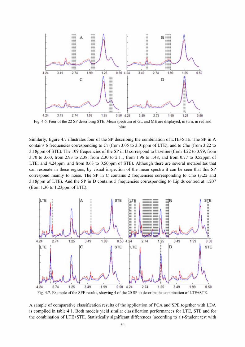
34

Similarly, figure 4.7 illustrates four of the SP describing the combination of LTE+STE. The SP in A contains 6 frequencies corresponding to Cr (from 3.05 to 3.01ppm of LTE); and to Cho (from 3.22 to 3.18ppm of STE). The 109 frequencies of the SP in B correspond to baseline (from 4.22 to 3.99, from 3.70 to 3.60, from 2.93 to 2.38, from 2.30 to 2.11, from 1.96 to 1.48, and from 0.77 to 0.52ppm of LTE; and 4.24ppm, and from 0.63 to 0.50ppm of STE). Although there are several metabolites that can resonate in these regions, by visual inspection of the mean spectra it can be seen that this SP correspond mainly to noise. The SP in C contains 2 frequencies corresponding to Cho (3.22 and 3.18ppm of LTE). And the SP in D contains 5 frequencies corresponding to Lipids centred at 1.207 (from 1.30 to 1.23ppm of LTE).

A sample of comparative classification results of the application of PCA and SPE together with LDA is compiled in table 4.1. Both models yield similar classification performances for LTE, STE and for the combination of LTE+STE. Statistically significant differences (according to a t-Student test with

Fig. 4.7. Example of the SPE results, showing 4 of the 20 SP to describe the combination of LTE+STE.

Fig. 4.6. Four of the 22 SP describing STE. Mean spectrum of GL and ME are displayed, in turn, in red and

blue.

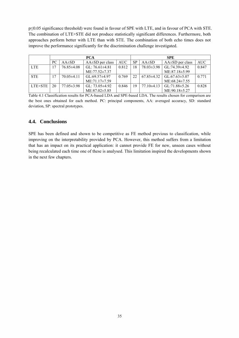
35

p≤0.05 significance threshold) were found in favour of SPE with LTE, and in favour of PCA with STE. The combination of LTE+STE did not produce statistically significant differences. Furthermore, both approaches perform better with LTE than with STE. The combination of both echo times does not improve the performance significantly for the discrimination challenge investigated.

PCA SPE

PC AA±SD AA±SD per class AUC SP AA±SD AA±SD per class AUC LTE 17 76.85±4.08 GL: 76.61±4.81

ME:77.52±7.37 0.812 18 78.03±3.98 GL:74.39±4.92

ME:87.18±5.99 0.847

STE 17 70.05±4.11 GL:69.57±4.97 ME:71.17±7.59

0.769 22 67.85±4.32 GL:67.63±5.07 ME:68.24±7.55

0.771

LTE+STE 20 77.05±3.98 GL: 73.05±4.92 ME:87.02±5.85

0.846 19 77.10±4.13 GL:71.88±5.26 ME:90.18±5.27

0.828

Table 4.1 Classification results for PCA-based LDA and SPE-based LDA. The results chosen for comparison are the best ones obtained for each method. PC: principal components, AA: averaged accuracy, SD: standard deviation, SP: spectral prototypes.

4.4. Conclusions

SPE has been defined and shown to be competitive as FE method previous to classification, while improving on the interpretability provided by PCA. However, this method suffers from a limitation that has an impact on its practical application: it cannot provide FE for new, unseen cases without being recalculated each time one of these is analysed. This limitation inspired the developments shown in the next few chapters.

37

5.

Assessing NMF for the spectral

decomposition of MRS data

5.1. Introduction

This chapter investigates the application of two FE techniques specifically suited to the problem of source extraction from signals, namely ICA [35] and NMF [36], to the analysis of SV 1H-MRS signal corresponding to several types of human brain tumours [15]. Previous exploratory investigations using ICA for the analysis of MRS data in neuro-oncology include those reported in [37, 38, 39] and [26]. In [37], two main signal types, closely resembling necrotic tumour tissue and actively proliferating, were identified. The capability of ICA to separate some tissue types was independently confirmed in [38] and [39]. In contrast, only in [37] and [26], the ICA results were used as a basis for ulterior classification. The NMF technique has previously been applied in a similar context to the analysis of source spectra from MR CSI data of the human brain [40] and to HR-MAS signals corresponding to brain tumours [41]. The comparative abilities of two variants of ICA and two variants of NMF, to identify the constituent tissue types in MRS from brain tumours collected in an international database, and for a number of different diagnostic problems, were preliminary investigated in [110]. In the current chapter, this preliminary analysis was extended in two ways, the first of which is by using synthetic data. These data are built from template sources (i.e. tissue averages), which are mixed using an example mixing matrix. The resulting data are then contaminated with different levels of uninformative noise and both ICA and NMF are used in an attempt to recover their true sources (which are known, due to their synthetic origin). This way, the robustness of the methods can be gauged in a far more general setting. The second extension of the analysis is to extend the benchmarking study with a more comprehensive set of variants of NMF. The experimental benchmarking study assesses also the differences between the sources extracted in these two different parameter settings, both of which are used in clinical practice.



The SV 1H-MRS data analysed in this chapter were extracted from the INTERPRET database [15], as described in chapter 3. Here, the analysed subset included, at LTE, 20 A2, 78 GL, 31 ME, 55 MM and 15 normal brain parenchyma measurements from healthy controls (NO); at STE, it included 22 A2, 86 GL, 38 ME, 58 MM, and 22 NO.

38

5.2.2. Selection of diagnostic problems

The variants of ICA and NMF under study in this chapter were applied to four diagnostic problems of interest, using data acquired both at LTE and STE; these were: A2 vs. NO; A2 vs. ME vs. NO; A2 vs. GL vs. NO; and A2 vs. MM vs. NO. Therefore, each of these problems attempts to discriminate between different tumour or tissue types. The label A2 indicates low-grade (grade II on a scale I-IV of the WHO [52]) glial tumours, which grow by infiltrating normal brain tissue. This class of tumoural masses may evolve to become highly malignant, WHO grade IV tumours, indicated by the label GL. So-called metastatic growths, ME, are also grade IV tumours, but they have a different origin. These are tumours with origin in other parts of the body that spread (metastasize) to distant sites, such as the brain. Grade IV tumours usually have a necrotic pattern where infiltrating tissue has died through lack of blood perfusion leaving behind strong lipid signals that are most evident when obtaining MRS data at short times of echo. However, not all GL have this necrotic pattern and some retain a spectral pattern which is visually not too different from their low-grade glial counterparts, the A2. These cases might be considered as class outliers [11, 104, 106, 27]. The label MM indicates low grade meningiomas (WHO grade I) and they have a completely different origin, namely cells in the tissue that envelops the brain, called the meninges. They have a distinct spectral pattern at long time of echo, with an inverted Ala doublet at ca.1.45 ppm. Their spectral pattern is also easy to recognise at short time of echo, without necrosis, and different from the glial, metastatic or normal pattern. Figure 5.1 shows the mean spectra of all the analysed tumour and tissue types, both at LTE and STE, across spectral ranges which follow acceptable clinical practice.

From a data processing point of view, the different class combinations represent classification tasks that range from relatively straightforward e.g. A2 vs. MM to difficult e.g. A2 vs. GL and A2 vs. ME. From a practical viewpoint, the choice of these specific problems at both acquisition conditions addresses to the following questions:

- A2 vs. NO: is normal brain correctly discriminated from infiltrating tumours? - A2 vs. ME vs. NO: are grades well distinguishable (WHO grades II vs. IV, vs. normal brain)? - A2 vs. GL vs. NO: are grades still well recognised when one of the classes is heterogeneous? - A2 vs. MM vs. NO. can low grades (A2 vs. MM, or II vs. I, or infiltrating vs. non-infiltrating)

be accurately differentiated?

Fig. 5.1. Mean spectra of the UL2 normalised tumour and tissue types at LTE (top row) and STE (bottom row). Frequencies in the horizontal axes measured in ppm; magnitudes in the vertical axis in arbitrary units.

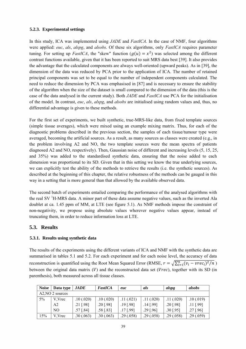
39

5.2.3. Experimental settings

In this study, ICA was implemented using JADE and FastICA. In the case of NMF, four algorithms were applied: euc, als, alspg, and alsobs. Of these six algorithms, only FastICA requires parameter tuning. For setting up FastICA, the "skew" function (𝑔(𝑢) = 𝑥2) was selected among the different contrast functions available, given that it has been reported to suit MRS data best [39]. It also provides the advantage that the calculated components are always well-oriented (upward peaks). As in [39], the dimension of the data was reduced by PCA prior to the application of ICA. The number of retained principal components was set to be equal to the number of independent components calculated. The need to reduce the dimension by PCA was emphasised in [87] and is necessary to ensure the stability of the algorithm when the size of the dataset is small compared to the dimension of the data (this is the case of the data analysed in the current study). Both JADE and FastICA use PCA for the initialisation of the model. In contrast, euc, als, alspg, and alsobs are initialised using random values and, thus, no differential advantage is given to these methods. For the first set of experiments, we built synthetic, true-MRS-like data, from fixed template sources (simple tissue averages), which were mixed using an example mixing matrix. Thus, for each of the diagnostic problems described in the previous section, the samples of each tissue/tumour type were averaged, becoming the artificial sources. As a result, as many sources as classes were created (e.g., in the problem involving A2 and NO, the two template sources were the mean spectra of patients diagnosed A2 and NO, respectively). Then, Gaussian noise of different and increasing levels (5, 15, 25, and 35%) was added to the standardised synthetic data, ensuring that the noise added to each dimension was proportional to its SD. Given that in this setting we know the true underlying sources, we can explicitly test the ability of the methods to retrieve the results (i.e. the synthetic sources). As described at the beginning of this chapter, the relative robustness of the methods can be gauged in this way in a setting that is more general than that allowed by the available observed data. The second batch of experiments entailed comparing the performance of the analysed algorithms with the real SV 1H-MRS data. A minor part of these data assume negative values, such as the inverted Ala doublet at ca. 1.45 ppm of MM, at LTE (see figure 5.1). As NMF methods impose the constraint of non-negativity, we propose using absolute values wherever negative values appear, instead of truncating them, in order to reduce information loss at LTE.

5.3. Results

5.3.1. Results using synthetic data

The results of the experiments using the different variants of ICA and NMF with the synthetic data are summarised in tables 5.1 and 5.2. For each experiment and for each noise level, the accuracy of data reconstruction is quantified using the Root Mean Squared Error (RMSE, 𝑟 = √∑ (𝑣𝑖 − 𝑣𝑟𝑒𝑐𝑖)2𝑛

𝑖=1 𝑛⁄ ) between the original data matrix (𝑉) and the reconstructed data set (𝑉𝑟𝑒𝑐), together with its SD (in parenthesis), both measured across all tissue classes.

Noise Data type JADE FastICA euc als alspg alsobs

A2,NO 2 sources 5% V,Vrec

A2 NO

.10 (.020)

.21 [.98]

.57 [.84]

.10 (.020)

.20 [.98]

.58 [.83]

.11 (.021)

.19 [.98]

.17 [.99]

.11 (.020)

.14 [.99]

.29 [.96]

.11 (.020)

.20 [.98]

.30 [.95]

.10 (.019)

.11 [.99]

.27 [.96] 15% V,Vrec .30 (.063) .30 (.063) .29 (.058) .29 (.058) .29 (.058) .29 (.059)

40

A2 NO

.21 [.98]

.57 [.84] .20 [.98] .58 [.83]

.20 [.98]

.18 [.98] .15 [.99] .30 [.96]

.20 [.98]

.31 [.95] .12 [.99] .28 [.96]

25% V,Vrec A2 NO

.57 (.114)

.21 [.98]

.57 [.84]

.57 (.114)

.21 [.98]

.57 [.84]

.56 (.110)

.20 [.98]

.18 [.98]

.56 (.109)

.17 [.99]

.27 [.96]

.56 (.110)

.21 [.98]

.29 [.96]

.56 (.110)

.13 [.99]

.25 [.97] 35% V,Vrec

A2 NO

.91 (.195)

.23 [.97]

.55 [.85]

.91 (.195)

.28 [.96]

.51 [.87]

.89 (.188)

.20 [.98]

.20 [.98]

.89 (.188)

.16 [.99]

.29 [.96]

.89 (.188)

.19 [.98]

.29 [.96]

.89 (.188)

.14 [.99]

.27 [.96] A2,ME,NO 3 sources 5% V,Vrec

A2 ME NO

.15 (.018)

.35 [.94]

.61 [.81]

.57 [.84]

.15 (.018)

.26 [.97]

.50 [.87]

.58 [.83]

.15 (.023)

.17 [.99]

.24 [.97]

.22 [.98]

.14 (.018)

.01 [1.0]

.43 [.91]

.22 [.98]

.15 (.018)

.29 [.96]

.43 [.91]

.25 [.97]

.14 (.018)

.25 [.97]

.43 [.91]

.23 [.97] 15% V,Vrec

A2 ME NO

.46 (.066)

.35 [.94]

.61 [.81]

.57 [.84]

.46 (.066)

.26 [.97]

.50 [.87]

.58 [.83]

.45 (.062)

.17 [.99]

.25 [.97]

.22 [.98]

.46 (.061)

.32 [.95]

.44 [.90]

.30 [.96]

.45 (.063)

.27 [.96]

.43 [.91]

.25 [.97]

.45 (.063)

.25 [.97]

.43 [.91]

.23 [.97] 25% V,Vrec

A2 ME NO

.86 (.109)

.35 [.94]

.62 [.81]

.57 [.83]

.86 (.109)

.26 [.97]

.50 [.87]

.58 [.83]

.82 (.090)

.18 [.98]

.24 [.97]

.22 [.98]

.82 (.089)

.27 [.96]

.37 [.93]

.30 [.96]

.82 (.090)

.25 [.97]

.42 [.91]

.26 [.97]

.82 (.090)

.22 [.98]

.42 [.91]

.24 [.97] 35% V,Vrec

A2 ME NO

1.35 (.173) .36 [.94] .63 [.80] .59 [.83]

1.35 (.173) .25 [.97] .50 [.87] .59 [.82]

1.29 (.159) .21 [.98] .28 [.96] .22 [.98]

1.29 (.159) .29 [.96] .41 [.92] .32 [.95]

1.29 (.159) .22 [.98] .40 [.92] .29 [.96]

1.29 (.159) .19 [.98] .40 [.92] .28 [.96]

A2,GL,NO 3 sources 5% V,Vrec

A2 GL NO

.14 (.018)

.33 [.95]

.60 [.82]

.57 [.84]

.14 (.018)

.24 [.97]

.70 [.75]

.58 [.83]

.17 (.028)

.25 [.97]

.36 [.94]

.22 [.98]

.16 (.022)

.33 [.94]

.78 [.69]

.30 [.96]

.14 (.015)

.30 [.96]

.76 [.71]

.23 [.97]

.14 (.016)

.26 [.97]

.75 [.72]

.22 [.98] 15% V,Vrec

A2 GL NO

.46 (.068)

.32 [.95]

.60 [.82]

.58 [.83]

.46 (.068)

.31 [.95]

.60 [.82]

.58 [.83]

.45 (.056)

.23 [.97]

.35 [.94]

.23 [.97]

.44 (.054)

.33 [.95]

.76 [.71]

.29 [.96]

.44 (.054)

.29 [.96]

.74 [.72]

.24 [.97]

.44 (.054)

.26 [.97]

.73 [.73]

.23 [.97] 25% V,Vrec

A2 GL NO

.83 (.105)

.32 [.95]

.62 [.81]

.56 [.84]

.83 (.105)

.31 [.95]

.61 [.81]

.58 [.83]

.81 (.089)

.23 [.97]

.36 [.93]

.24 [.97]

.80 (.089)

.32 [.95]

.80 [.68]

.27 [.96]

.80 (.089)

.29 [.96]

.78 [.70]

.24 [.97]

.80 (.089)

.27 [.96]

.77 [.70]

.23 [.97] 35% V,Vrec

A2 GL NO

1.31 (.160) .31 [.95] .62 [.81] .57 [.84]

1.31 (.160) .35 [.94] .62 [.81] .53 [.86]

1.27 (.143) .27 [.96] .38 [.93] .24 [.97]

1.27 (.142) .32 [.95] .82 [.66] .28 [.96]

1.27 (.142) .30 [.96] .80 [.68] .26 [.97]

1.27 (.142) .27 [.96] .78 [.69] .25 [.97]

A2,MM,NO 3 sources 5% V,Vrec

A2 MM NO

.11 (.018)

.38 [.93]

.20 [.98]

.58 [.83]

.11 (.018)

.38 [.93]

.18 [.98]

.59 [.83]

.15 (.037)

.55 [.85]

.22 [.98]

.49 [.88]

.19 (.059)

.44 [.90]

.32 [.95]

.45 [.90]

.12 (.019)

.39 [.92]

.21 [.98]

.41 [.91]

.12 (.018)

.37 [.93]

.21 [.98]

.44 [.90] 15% V,Vrec

A2 MM NO

.35 (.060)

.39 [.92]

.18 [.98]

.59 [.83]

.35 (.060)

.43 [.91]

.19 [.98]

.54 [.85]

.35 (.057)

.55 [.85]

.21 [.98]

.49 [.88]

.36 (.054)

.57 [.84]

.20 [.98]

.42 [.91]

.34 (.055)

.37 [.93]

.20 [.98]

.41 [.92]

.34 (.055)

.34 [.94]

.20 [.98]

.43 [.91]

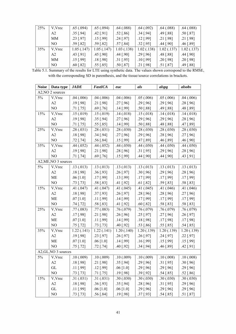
41

25% V,Vrec A2 MM NO

.65 (.094)

.35 [.94]

.23 [.97]

.59 [.82]

.65 (.094)

.42 [.91]

.15 [.99]

.59 [.82]

.64 (.088)

.52 [.86]

.24 [.97]

.57 [.84]

.64 (.092)

.34 [.94]

.12 [.99]

.32 [.95]

.64 (.088)

.49 [.88]

.21 [.98]

.44 [.90]

.64 (.088)

.50 [.87]

.21 [.98]

.46 [.89] 35% V,Vrec

A2 MM NO

1.05 (.147) .43 [.91] .15 [.99] .60 [.82]

1.05 (.147) .45 [.90] .18 [.98] .55 [.85]

1.03 (.138) .44 [.90] .31 [.95] .50 [.87]

1.02 (.138) .29 [.96] .10 [.99] .21 [.98]

1.02 (.137) .48 [.88] .20 [.98] .51 [.87]

1.02 (.137) .44 [.90] .20 [.98] .49 [.88]

Table 5.1. Summary of the results for LTE using synthetic data. The values shown correspond to the RMSE, with the corresponding SD in parenthesis, and the tissue/source correlations in brackets.

Noise Data type JADE FastICA euc als alspg alsobs

A2,NO 2 sources

5% V,Vrec A2 NO

.04 (.006)

.19 [.98]

.71 [.75]

.04 (.006)

.21 [.98]

.69 [.76]

.04 (.006)

.27 [.96]

.14 [.99]

.05 (.006)

.29 [.96]

.50 [.88]

.05 (.006)

.29 [.96]

.49 [.88]

.04 (.006)

.28 [.96]

.48 [.89] 15% V,Vrec

A2 NO

.15 (.019)

.19 [.98]

.71 [.75]

.15 (.019)

.35 [.94]

.55 [.85]

.14 (.018)

.27 [.96]

.14 [.99]

.15 (.018)

.29 [.96]

.50 [.88]

.14 (.018)

.29 [.96]

.48 [.88]

.14 (.018)

.28 [.96]

.47 [.89] 25% V,Vrec

A2 NO

.28 (.031)

.18 [.98]

.72 [.74]

.28 (.031)

.34 [.94]

.56 [.84]

.28 (.030)

.27 [.96]

.15 [.99]

.28 (.030)

.29 [.96]

.47 [.89]

.28 (.030)

.28 [.96]

.46 [.89]

.28 (.030)

.27 [.96]

.46 [.90] 35% V,Vrec

A2 NO

.44 (.052)

.19 [.98]

.71 [.74]

.44 (.052)

.21 [.98]

.69 [.76]

.44 (.050)

.28 [.96]

.15 [.99]

.44 (.050)

.31 [.95]

.44 [.90]

.44 (.050)

.29 [.96]

.44 [.90]

.44 (.050)

.28 [.96]

.43 [.91] A2,ME,NO 3 sources 5% V,Vrec

A2 ME NO

.13 (.013)

.18 [.98]

.06 [1.0]

.73 [.73]

.13 (.013)

.36 [.93]

.17 [.99]

.58 [.83]

.13 (.013)

.26 [.97]

.13 [.99]

.41 [.92]

.13 (.013)

.30 [.96]

.17 [.99]

.61 [.82]

.13 (.013)

.29 [.96]

.17 [.99]

.59 [.83]

.13 (.013)

.28 [.96]

.17 [.99]

.58 [.83] 15% V,Vrec

A2 ME NO

.41 (.047)

.18 [.98]

.07 [1.0]

.74 [.72]

.41 (.047)

.37 [.93]

.11 [.99]

.58 [.83]

.41 (.045)

.26 [.97]

.14 [.99]

.41 [.92]

.41 (.045)

.28 [.96]

.17 [.99]

.60 [.82]

.41 (.046)

.28 [.96]

.17 [.99]

.58 [.83]

.41 (.046)

.27 [.96]

.17 [.99]

.58 [.83] 25% V,Vrec

A2 ME NO

.77 (.083)

.17 [.98]

.07 [1.0]

.75 [.72]

.77 (.083)

.21 [.98]

.11 [.99]

.73 [.73]

.76 (.079)

.26 [.96]

.14 [.99]

.40 [.92]

.76 (.079)

.25 [.97]

.18 [.98]

.53 [.86]

.76 (.079)

.27 [.96]

.17 [.98]

.55 [.85]

.76 (.079)

.26 [.97]

.17 [.98]

.54 [.85] 35% V,Vrec

A2 ME NO

1.22 (.141) .19 [.98] .07 [1.0] .75 [.72]

1.22 (.141) .23 [.97] .06 [1.0] .72 [.74]

1.20 (.140) .26 [.97] .14 [.99] .40 [.92]

1.20 (.139) .26 [.97] .16 [.99] .34 [.94]

1.20 (.139) .24 [.97] .15 [.99] .46 [.89]

1.20 (.139) .22 [.97] .15 [.99] .42 [.91]

A2,GL,NO 3 sources 5% V,Vrec

A2 GL NO

.10 (.009)

.18 [.98]

.11 [.99]

.73 [.73]

.10 (.009)

.21 [.98]

.12 [.99]

.71 [.75]

.10 (.009)

.35 [.94]

.06 [1.0]

.19 [.98]

.10 (.009)

.29 [.96]

.29 [.96]

.39 [.92]

.10 (.008)

.31 [.95]

.29 [.96]

.54 [.85]

.10 (.008)

.30 [.96]

.29 [.96]

.52 [.86] 15% V,Vrec

A2 GL NO

.31 (.031)

.18 [.98]

.11 [.99]

.73 [.73]

.31 (.031)

.36 [.93]

.06 [1.0]

.56 [.84]

.30 (.030)

.35 [.94]

.06 [1.0]

.19 [.98]

.30 (.030)

.28 [.96]

.29 [.96]

.37 [.93]

.30 (.030)

.31 [.95]

.29 [.96]

.54 [.85]

.30 (.030)

.29 [.96]

.29 [.96]

.51 [.87]

42

25% V,Vrec A2 GL NO

.59 (.054)

.18 [.98]

.11 [.99]

.73 [.73]

.59 (.054)

.21 [.98]

.19 [.98]

.73 [.73]

.58 (.052)

.35 [.94]

.06 [1.0]

.19 [.98]

.58 (.052)

.27 [.96]

.29 [.96]

.33 [.95]

.58 (.052)

.30 [.96]

.29 [.96]

.54 [.85]

.58 (.052)

.28 [.96]

.29 [.96]

.50 [.87] 35% V,Vrec

A2 GL NO

.92 (.095)

.18 [.98]

.12 [.99]

.74 [.72]

.92 (.095)

.21 [.98]

.08 [1.0]

.71 [.75]

.91 (.093)

.34 [.94]

.07 [1.0]

.19 [.98]

.91 (.093)

.27 [.96]

.28 [.96]

.27 [.96]

.91 (.093)

.29 [.96]

.28 [.96]

.48 [.88]

.91 (.093)

.28 [.96]

.28 [.96]

.45 [.90] A2,MM,NO 3 sources 5% V,Vrec

A2 MM NO

.06 (.006)

.40 [.92]

.40 [.92]

.72 [.74]

.06 (.006)

.48 [.88]

.41 [.92]

.62 [.81]

.06 (.006)

.25 [.97]

.47 [.89]

.23 [.97]

.06 (.006)

.35 [.94]

.54 [.85]

.23 [.97]

.06 (.006)

.33 [.95]

.47 [.89]

.65 [.79]

.06 (.006)

.36 [.94]

.58 [.83]

.21 [.98] 15% V,Vrec

A2 MM NO

.20 (.017)

.40 [.92]

.40 [.92]

.72 [.74]

.20 (.017)

.43 [.91]

.40 [.92]

.70 [.76]

.20 (.017)

.24 [.97]

.46 [.89]

.23 [.97]

.20 (.017)

.35 [.94]

.55 [.85]

.22 [.98]

.20 (.017)

.32 [.95]

.45 [.90]

.63 [.80]

.20 (.016)

.35 [.94]

.54 [.85]

.23 [.97] 25% V,Vrec

A2 MM NO

.38 (.036)

.42 [.91]

.38 [.93]

.73 [.74]

.38 (.036)

.44 [.90]

.39 [.92]

.70 [.75]

.38 (.036)

.25 [.97]

.47 [.89]

.23 [.97]

.38 (.036)

.35 [.94]

.55 [.85]

.20 [.98]

.38 (.036)

.32 [.95]

.45 [.90]

.63 [.80]

.38 (.036)

.35 [.94]

.54 [.85]

.21 [.98] 35% V,Vrec

A2 MM NO

.61 (.053)

.44 [.90]

.37 [.93]

.73 [.73]

.61 (.053)

.50 [.88]

.39 [.92]

.63 [.80]

.60 (.052)

.26 [.96]

.47 [.89]

.24 [.97]

.60 (.052)

.31 [.95]

.52 [.87]

.22 [.98]

.60 (.052)

.32 [.95]

.45 [.90]

.61 [.81]

.60 (.052)

.31 [.95]

.45 [.90]

.61 [.81] Table 5.2. Summary of the results for STE using synthetic data, reported as in the previous table.

The second evaluation quantifies the accuracy with which the original sources are recovered. This is measured by the RMSE and the correlation (in brackets) between the mean spectrum of each tissue type and the closest extracted source signal. This measure provides an important indication of the extent to which each source is tissue type-specific.

5.3.2. Results using INTERPRET data

The results of the analysis of INTERPRET data, using all variants of ICA and NMF, are compiled in tables 5.3 and 5.4. As for the experiments with synthetic data, the RMSE between the original and reconstructed dataset and its SD were calculated. The RMSE and the correlation between the mean spectrum of each tissue type and the source signal that represents it the most were also calculated. Graphical illustrations of the sources extracted with ICA and NMF in all the analysed variants can be found in figures 5.2 and 5.3. They correspond to two of the investigated problems: A2 vs. ME vs. NO with data acquired at LTE (figure 5.2) and A2 vs. GL vs. NO with data acquired at STE (figure 5.3). The sources in the first row (of both figures) seem to represent the actively proliferating tumour, for which the high levels of total choline are a clear indicator; the ones in the second row appear to correspond to necrotic core sources, as evidenced by the presence of high levels of ML; finally, the ones in the third row are clearly representing normal brain sources, as suggested by the simultaneous high levels of N-acetyl aspartate (NAA), total Cr, and Cho. Similar results were also found for the other three problems (that is, very stable sources regardless both the problem and the spectral decomposition method used).

43

Data type JADE FastICA euc als alspg alsobs

A2,NO 2 sources

V,Vrec A2 NO

2.45(.766) .22[.98] .56[.84]

2.45(.766) .21[.98] .57[.83]

2.10(.644) .30[.97] .27[.98]

2.10(.644) .30[.96] .36[.95]

2.10(.644) .30[.97] .36[.95]

2.10(.644) .30[.97] .36[.95]

A2,ME,NO 3 sources V,Vrec A2 ME NO

2.62(.889) .42[.91] .64[.80] .52[.87]

2.62(.889) .45[.90] .64[.79] .48[.88]

2.19(.720) .35[.93] .58[.81] .20[.99]

2.19(.720) .34[.94] .58[.81] .42[.91]

2.19(.720) .34[.93] .57[.81] .27[.98]

2.19(.720) .34[.93] .57[.81] .27[.98]

A2,GL,NO 3 sources V,Vrec A2 GL NO

2.63(.861) .44[.90] .56[.84] .52[.86]

2.63(.861) .44[.90] .56[.84] .53[.86]

2.21(.619) .40[.91] .52[.77] .21[.99]

2.21(.621) .40[.91] .52[.78] .32[.95]

2.21(.619) .40[.91] .51[.77] .22[.99]

2.21(.619) .40[.91] .51[.77] .25[.98]

A2,MM,NO 3 sources V,Vrec A2 MM NO

2.81(.974) .36[.94] .28[.96] .54[.85]

2.81(.974) .55[.85] .11[.99] .51[.87]

2.36(.609) .51[.85] .33[.98] .21[.98]

2.35(.594) .45[.88] .35[.97] .21[.98]

2.35(.594) .46[.87] .35[.97] .21[.98]

2.35(.594) .46[.87] .35[.97] .21[.98]

Table 5.3. Summary of the results for LTE using data from the INTERPRET database, reported as in the previous tables.

Data type JADE FastICA euc als alspg alsobs

A2,NO 2 sources

V,Vrec A2 NO

1.91(.892) .26[.97] .68[.77]

1.91(.892) .27[.96] .67[.78]

1.57(.592) .25[.93] .34[.94]

1.57(.592) .27[.92] .44[.86]

1.57(.592) .27[.92] .34[.94]

1.57(.592) .27[.92] .35[.94]

A2,ME,NO 3 sources V,Vrec A2 ME NO

1.78(.728) .37[.93] .10[.99] .66[.78]

1.78(.728) .34[.94] .12[.99] .70[.75]

1.48(.533) .33[.94] .17[.98] .48[.77]

1.48(.531) .34[.93] .17[.98] .47[.74]

1.48(.534) .34[.93] .17[.98] .46[.69]

1.48(.534) .34[.93] .17[.98] .46[.69]

A2,GL,NO 3 sources V,Vrec A2 GL NO

1.75(.735) .36[.94] .16[.99] .69[.76]

1.75(.735) .38[.93] .19[.98] .68[.77]

1.46(.537) .32[.93] .26[.95] .43[.88]

1.46(.536) .36[.89] .26[.94] .46[.83]

1.46(.537) .35[.90] .26[.95] .45[.84]

1.46(.537) .35[.90] .26[.95] .47[.80]

A2,MM,NO 3 sources V,Vrec A2 MM NO

2.09(.624) .39[.92] .75[.72] .69[.76]

2.09(.624) .55[.85] .56[.84] .60[.82]

1.74(.522) .30[.92] .76[.59] .39[.92]

1.74(.517) .32[.92] .75[.58] .53[.77]

1.74(.516) .33[.91] .75[.58] .53[.79]

1.74(.516) .33[.92] .75[.58] .53[.79]

Table 5.4. Summary of the results for STE using data from the INTERPRET database, reported as in the previous tables.

44

5.4. Discussion

5.4.1. NMF vs. ICA

In the case of ICA, only small differences were found between the results obtained with the JADE and FastICA implementations. On the contrary, the four NMF implementations seem to differ more significantly in their results, euc being the best overall performing variant, followed by als and alspg. This differential advantage of euc is clear in terms of lower RMSE for each tissue/tumour type and, in general, higher (and, importantly, more homogeneous) correlations with tissue/tumour types. The alsobs algorithm, in particular, yields rather poor results for some problems.

Fig. 5.3. Three source signals as obtained with the six spectral decomposition algorithms for the problem A2, GL, NO with STE data. First row: actively proliferating tumor; second row: necrotic core; and third row: normal brain sources. See figure 5.2 legend for further details.

Fig. 5.2. Three source signals as obtained with the six spectral decomposition algorithms for the problem A2, ME, NO with LTE data. First row: actively proliferating tumour; second row: necrotic core; and third row: normal brain sources. See text and [11, 13] for further details.

45

Both in terms of errors and correlations (as reported in tables 5.1, 5.2, 5.3 and 5.4), the results obtained with NMF are, in general, better than those obtained with ICA, with both synthetic and real data, especially when added noise increases. This would suggest robustness when faced with real-life data (see section 5.4.2). The two only exceptions to be found are: first, in the problem of discriminating between A2, MM and NO using the INTERPRET data, where JADE yields lower error and higher correlation for A2 at LTE and FastICA for MM at STE; second, in the differentiation between A2, GL and NO from INTERPRET data at LTE, where both variants of ICA yield better correlations for the high-grade GL.

5.4.2. Synthetic vs. real data and the presence of noise

The results obtained with the INTERPRET data compare unfavourably with those obtained with the synthetic data. This is clear in terms of RMSE, but also in terms of correlation between the extracted sources and the tumour/tissue types, especially in problems where high-grade tumours are included. This is due to the high heterogeneity of these tumours in the INTERPRET dataset. The differences in performance are consistent for both ICA and NMF and for all their variants. From the results for synthetic data, all methods are shown to behave very robustly in the presence of uninformative noise.

5.4.3. LTE vs. STE

The reported results, both for synthetic and real INTERPRET data, reveal that the convenience of using data acquired at either LTE or STE is clearly problem-dependent. STE seems to provide better accuracy results when high-grade malignant tumours (GL and ME) are involved, whereas LTE shows some advantage in problems involving NO, low-grade gliomas (A2) and meningiomas (MM).

5.4.4. Source signals

Most importantly, the obtained source signals can be interpreted biomedically. We have illustrated this in figures 5.2 and 5.3 with the sources obtained for two of the analysed problems (A2, ME, NO at LTE and A2, GL, NO at STE). The three sources represented in both figures can be associated to the following tissue types: actively proliferating tumour, necrotic core, and normal brain. Spectra acquired from healthy tissue mainly contain high levels of NAA, Cho and Cr. The NAA peaks can be observed at 2.02 and 2.61ppm. The creatine and phosphocreatine (usually named "total Cr") generate a signal at 3.03ppm, and also at 3.93ppm if good water suppression has been achieved. The signal from Cho and other choline-containing compounds such as phosphocholine and glycerophosphocholine appears at 3.21ppm. Generally speaking, the NAA level decreases in tumours, while the Cho level increases. In aggressive tumours and necrosis, peaks of Lac and ML can appear as a result of anaerobic metabolism. The strong signal from Lac and the methylen group of ML appears centred at 1.30 ppm. Figures 5.2 and 5.3 also reveal the similarities of the sources obtained with the different methods. The most eye-catching difference is found in the sources representing the normal brain (in the last row) at LTE (figure 5.2), where the patterns obtained with the NMF techniques (and very especially with euc) look closer to the normal brain mean pattern than the ICA ones (compare, for instance, with the double Cho and creatine peaks of the NO average depicted in figure 5.1). In table 5.3, this corresponds with the correlation values of NO, which are higher for NMF than for ICA, as previously mentioned.

5.5. Conclusions

The use of NMF for the analysis of MRS information, especially when using the euc algorithm variant, has shown some advantages over ICA in terms of the overall good tumour-type specificity of its

46

obtained sources (as measured by the correlations between these sources and the analysed tumour types) and, more specifically, in its capability to find sources clearly compatible with recognisable and radiologically interpretable patterns such as actively proliferating tumour, necrotic core sources, and normal brain. The obtained results also show the ability of these methods, and specially NMF, to discriminate between normal brain and infiltrating tumour, as expressed by the high correlations at LTE and STE. As an answer to the questions posed in section 5.2, we can conclude that both low grade infiltrating tumour and normal brain have been shown to be well distinguishable from high grade tumours, as expressed by the high correlations found for low grade and normal brain at LTE and for the high grade tumours at STE. Non-infiltrative tumours can also be well differentiated, especially at STE.

47

6.

Convex-NMF for the analysis of

single-voxel MRS data

6.1. Introduction

In this chapter, we investigate the performance of a range of variants of NMF with real MRS data in two respects: first, to derive sources correlated with the mean spectra of known tissue types; second, taking the best performing NMF method for source separation, we compare its accuracy for class assignment when using the mixing matrix directly as a basis for classification, as against using the method for DR. This method is unsupervised in the sense that labelled cases are not required to create a model of the analysed MRS data (i.e., to find the MRS sources). The results reported in the current chapter reveal the advantage of using one of the recently described NMF variants, namely Convex-NMF [42], as an unsupervised method of source extraction from SV 1H-MRS. In contrast with ICA, most of the sources extracted by the proposed technique closely correspond to the mean spectra of some of the analysed tumour types. This similarity allows accurate diagnostic predictions to be made for each patient (that is, for each SV spectrum) both in fully unsupervised mode or using Convex-NMF as a DR step previous to standard supervised classification. These predictions are comparable to or more accurate than those obtained with supervised techniques.



The SV 1H-MRS data analysed in this chapter were also extracted from the INTERPRET database [15]. It included the same subset of A2, GL, ME, MM and NO, described in the previous chapter, at both LTE and STE. A further test data set was gathered from three medical centres: Centre Diagnòstic Pedralbes (CDP), Institut d'Alta Tecnologia (IAT) and Institut de Diagnòstic per la Imatge (IDI)-Badalona in Barcelona, Spain. It was processed in the same conditions as the rest of the data, and consists of STE and LTE spectra from 56 patients and healthy controls: 10 A2, 40 high-grade aggressive tumours (30 GL + 10 ME), 3 MM, and 3 NO subjects.

6.2.2. Interpretation of the methods

In NMF for the analysis of MRS data, the rows in 𝐻 (see Eq. 2.1) can be understood as estimates of the concentration/abundance of the constituent signals or sources, while the columns in 𝑊 (also in Eq. 2.1) are the corresponding constituent signals or sources of the spectra themselves. In conventional NMF methods (such as euc, als, alspg, and alsobs), the matrices 𝑉, 𝑊 and 𝐻 are constrained to be

48

non-negative, thus permitting the interpretation of the mixing matrix entries as quantitative estimates of the amount of source tissue in the sample. The source can, as a result, be assigned to the class (tumour type or healthy tissue) with whose template it shows a higher correlation. If non-negativity is also imposed on the signals and sources, it is then commonplace truncating the negative values to zero, therefore loosing potentially relevant information (for instance, Lac, Ala, and Glx) in spectra at LTE, which are expected to be especially relevant for discrimination between tumour types. Some of the methods described above impose the constraint of non-negativity only on the mixing elements representing the constituent tissue fractions. Where non-negative signals are also required, we propose using absolute values instead, in order to reduce data loss from the negative peaks. Convex-NMF, instead, enforces this non-negative constraint only on 𝐻, while 𝑉 and 𝑊 are allowed to be of mixed sign. Given that the observed MRS data are of mixed sign, we should expect their sources also to be of mixed sign. Thus, understanding 𝑊 as the source spectra matrix, the sources will be intuitively interpretable and no ad hoc pre-processing of the spectra is required in order to make them non-negative, thus preventing any unnecessary loss of information (in the case of our database, losing the information in the negative peaks of the MRS LTE spectra). As in the previous methods, the values in 𝐻 can be understood as estimates of the concentration/abundance of the constituent signals.

6.2.3. NMF initialisations

NMF methods unavoidably converge to local minima. As a result, the extracted NMF bases will be different for different initialisations. In this thesis, six initialisation methods were investigated, covering a wide array of approaches: from random initialisation, to prototype-based clustering methods such as K-means and Fuzzy C-Means (FCM), which provide a data density-based sample of initial data locations; and to feature extraction techniques such as Principal Component Analysis (PCA), ICA and NMF itself, which initialise the algorithm according to the basic eigenstructure of the data.

Random: [all methods]: 𝑊 and 𝐻 are initialised as dense matrices of random values between 0 and 1.

K-means clustering: [euc, alspg, als, alsobs]: 𝑊 is initialised with the cluster centroids, and 𝐻 with the distances from each point (MR spectrum) to every centroid. [convex]: 𝐻 is initialised as 𝐻(0) = 𝐶 + 0.2𝐸 , where 𝐸 is a matrix with all its elements equal to one, and 𝐶 = (𝑐1, ⋯ , 𝑐𝑛) is filled with the cluster indicators, which are based on the cluster indices of each point, such that 𝐶𝑖𝑘 = {0,1} and the ones indicate cluster membership. 𝐴 is initialised as 𝐴(0) = (𝐶 + 0.2𝐸)𝐷−1, where 𝐷 is a diagonal matrix with each element being the number of points in each cluster [42].

Fuzzy C-Means (FCM): [euc, alspg, als, alsobs]: 𝑊 is initialised with the cluster centres, and 𝐻 with the fuzzy partition matrix (or membership function matrix); as in [111]. [convex]: 𝐻 is initialised as 𝐻(0) = 𝐶 + 0.2𝐸, where 𝐶 here is filled with the fuzzy partition values, and 𝐸 is a matrix with all its elements equal to one. 𝐴 is initialised as 𝐴(0) = (𝐶 +

0.2𝐸)𝐷−1, where 𝐷 is a diagonal matrix with each element being the number of points in each cluster.

PCA: [euc, alspg, als, alsobs]: The mean vector is subtracted from the complete dataset, and this is followed by the computation of its eigenvectors and eigenvalues. The matrix 𝑊 is

49

initialised with the whitened data (the corresponding projection of the eigenvectors), and 𝐻 with the de-whitening matrix. In order to use the initial 𝑊 and 𝐻 matrices obtained from PCA in NMF, the negative values are truncated, as proposed in [111]. [convex]: 𝐻 is initialised as 𝐻(0) = 𝐶 + 0.2𝐸 , where 𝐶 is the de-whitening matrix, calculated, as in the rest of methods, after calculating PCA, and also truncating the negative values. For the initialisation of 𝐴 , and as suggested in [42], first we compute 𝐴 =

𝐻𝑇(𝐻𝐻𝑇)−1, and then 𝐴(0) = 𝐴+ + 0.2𝐸⟨𝐴+⟩ so that the negative elements are removed, where ⟨𝑋⟩ = ∑ |𝑋𝑛,𝑘| ‖𝑋𝑛,𝑘‖

0⁄𝑛,𝑘 , and where ‖𝑋𝑛,𝑘‖

0 is the number of nonzero elements in

𝑋.

ICA (FastICA [87] algorithm): [euc, alspg, als, alsobs]: The independent components extracted using FastICA are used to initialise 𝑊, and 𝐻 is initialised with the resulting mixing matrix. Then, to meet the non-negativity condition of NMF, the negative values are truncated. [convex]: 𝐻 and 𝐴 are initialised as in the PCA (for convex) initialisation, with the only difference that 𝐻 is filled with the sources or independent components from FastICA.

Non-negative Matrix Factorisation (NMF, als algorithm): [euc, alspg, als, alsobs]: 𝑊 is initialised with the sources extracted with NMF (als), and 𝐻 is initialised with the resulting mixing matrix. In the case of als method, initialising with the same method is equivalent to duplicating the number of iterations, which does not necessarily mean that the results will improve. [convex]: 𝐻 and 𝐴 are initialised as in the PCA and FastICA (for convex) initialisations, with the only difference that 𝐻 is filled with the sources from NMF (als).

In principle, we might expect the different initialisation strategies to behave as follows. Random initialisation might be considered as an uninformed first estimate for NMF methods, which may lead to different outcomes given different initialisation conditions [111, 112]. We might expect K-means and FCM initialisations to make all methods perform better, but the results may depend on the initial selection of clusters; therefore, different results could be obtained depending on such selection. PCA and ICA, instead, can provide a unique solution, although perhaps too biased, while, in the case of NMF, the existence of a unique solution will depend on its own initialisation. All the NMF algorithms, for all initialisations, were allowed to achieve convergence. Convergence was qualified as the lack of variation in the reconstruction error, from one iteration to the next, over a common set small threshold of value 10-5.

6.2.4. Labelling using the mixing matrix and the sources

NMF in this thesis is used as an unsupervised method in the sense that labelled spectra are not used to create the data model. The obvious advantage of this approach lies in the fact that the labelling procedure becomes independent of the availability of labelled MRS datasets. Two further advantages come with this independence: First, the generalisation capabilities of the obtained model will not be compromised by the bias introduced by the finite size of the labelled sample. Second, the negative effect of mislabelled cases on the generalisation capabilities of the model will be prevented. In order to represent the data using the source signals obtained through the chosen NMF method, we propose to infer the labels of each patient case only on the basis of the mixing matrix and the calculated source signals, which will give us an idea of the extent to which each of the sources contributes to the reconstruction of each MRS observation (or patient case). The calculation of the

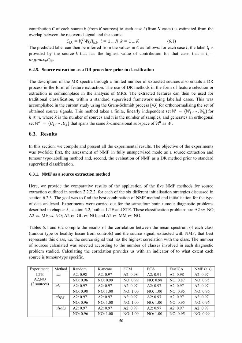
50

contribution 𝐶 of each source 𝑘 (from 𝐾 sources) to each case 𝑖 (from 𝑁 cases) is estimated from the overlap between the recovered signal and the source:

𝐶𝑖,𝑘 = 𝑉𝑖𝑇𝑊𝑘𝐻𝑘,𝑖, 𝑖 = 1 … 𝑁, 𝑘 = 1 … 𝐾 (6.1)

The predicted label can then be inferred from the values in 𝐶 as follows: for each case 𝑖, the label 𝑙𝑖 is provided by the source 𝑘 that has the highest value of contribution for that case, that is 𝑙𝑖 =

𝑎𝑟𝑔𝑚𝑎𝑥𝑘𝐶𝑖𝑘.

6.2.5. Source extraction as a DR procedure prior to classification

The description of the MR spectra through a limited number of extracted sources also entails a DR process in the form of feature extraction. The use of DR methods in the form of feature selection or extraction is commonplace in the analysis of MRS. The extracted features can then be used for traditional classification, within a standard supervised framework using labelled cases. This was accomplished in the current study using the Gram-Schmidt process [43] for orthonormalising the set of obtained source signals. This method takes a finite, linearly independent set 𝑊 = {𝑊1, ⋯ , 𝑊𝑘} for 𝑘 ≤ 𝑛, where 𝑘 is the number of sources and 𝑛 is the number of samples, and generates an orthogonal set 𝑊′ = {𝑈1, ⋯ , 𝑈𝑘} that spans the same 𝑘-dimensional subspace of ℜ𝑛 as 𝑊.

6.3. Results

In this section, we compile and present all the experimental results. The objective of the experiments was twofold: first, the assessment of NMF in fully unsupervised mode as a source extraction and tumour type-labelling method and, second, the evaluation of NMF as a DR method prior to standard supervised classification.

6.3.1. NMF as a source extraction method

Here, we provide the comparative results of the application of the five NMF methods for source extraction outlined in section 2.2.2.2, for each of the six different initialisation strategies discussed in section 6.2.3. The goal was to find the best combination of NMF method and initialisation for the type of data analysed. Experiments were carried out for the same four brain tumour diagnostic problems described in chapter 5, section 5.2, both at LTE and STE. These classification problems are A2 vs. NO; A2 vs. ME vs. NO; A2 vs. GL vs. NO; and A2 vs. MM vs. NO. Tables 6.1 and 6.2 compile the results of the correlation between the mean spectrum of each class (tumour type or healthy tissue from controls) and the source signal, extracted with NMF, that best represents this class, i.e. the source signal that has the highest correlation with the class. The number of sources calculated was selected according to the number of classes involved in each diagnostic problem studied. Calculating the correlation provides us with an indicator of to what extent each source is tumour-type specific. Experiment Method Random K-means FCM PCA FastICA NMF (als)

LTE A2,NO

(2 sources)

euc A2: 0.98 A2: 0.97 A2: 0.98 A2: 0.91 A2: 0.98 A2: 0.97 NO: 0.96 NO: 0.99 NO: 0.99 NO: 0.98 NO: 0.87 NO: 0.95

als A2: 0.97 A2: 0.97 A2: 0.97 A2: 0.97 A2: 0.97 A2: 0.97 NO: 0.98 NO: 1.00 NO: 1.00 NO: 1.00 NO: 0.95 NO: 0.96

alspg A2: 0.97 A2: 0.97 A2: 0.97 A2: 0.97 A2: 0.97 A2: 0.97 NO: 0.96 NO: 1.00 NO: 1.00 NO: 1.00 NO: 0.95 NO: 0.96

alsobs A2: 0.97 A2: 0.97 A2: 0.97 A2: 0.97 A2: 0.97 A2: 0.97 NO: 0.96 NO: 1.00 NO: 1.00 NO: 1.00 NO: 0.95 NO: 0.99

51

convex A2: 1.00 A2: 1.00 A2: 1.00 A2: 0.99 A2: 1.00 A2: 1.00 NO: 1.00 NO: 1.00 NO: 1.00 NO: 1.00 NO: 1.00 NO: 1.00

LTE A2,ME,NO (3 sources)

euc A2: 0.94 A2: 0.94 A2: 0.94 A2: 0.88 A2: 0.94 A2: 0.94 ME: 0.85 ME: 0.85 ME: 0.85 ME: 0.78 ME: 0.86 ME: 0.85 NO: 0.95 NO: 1.00 NO: 0.99 NO: 0.90 NO: 0.92 NO: 0.93

als A2: 0.94 A2: 0.94 A2: 0.94 A2: 0.94 A2: 0.94 A2: 0.94 ME: 0.85 ME: 0.84 ME: 0.84 ME: 0.85 ME: 0.85 ME: 0.85 NO: 0.92 NO: 0.99 NO: 0.99 NO: 0.92 NO: 0.91 NO: 0.91

alspg A2: 0.94 A2: 0.94 A2: 0.94 A2: 0.94 A2: 0.94 A2: 0.94 ME: 0.85 ME: 0.85 ME: 0.85 ME: 0.85 ME: 0.85 ME: 0.85 NO: 0.99 NO: 0.99 NO: 0.99 NO: 0.95 NO: 0.93 NO: 0.92

alsobs A2: 0.94 A2: 0.94 A2: 0.94 A2: 0.94 A2: 0.94 A2: 0.94 ME: 0.85 ME: 0.85 ME: 0.85 ME: 0.85 ME: 0.85 ME: 0.85 NO: 0.96 NO: 0.99 NO: 0.99 NO: 0.95 NO: 0.95 NO: 0.95

convex A2: 0.99 A2: 0.99 A2: 0.98 A2: 0.98 A2: 0.98 A2: 0.98 ME: 0.88 ME: 0.88 ME: 0.90 ME: 0.86 ME: 0.87 ME: 0.87 NO: 1.00 NO: 1.00 NO: 1.00 NO: 1.00 NO: 1.00 NO: 1.00

LTE A2,GL,NO (3 sources)

euc A2: 0.91 A2: 0.91 A2: 0.91 A2: 0.87 A2: 0.92 A2: 0.91 GL: 0.75 GL: 0.76 GL: 0.75 GL: 0.92 GL: 0.78 GL: 0.76 NO: 0.99 NO: 0.99 NO: 0.99 NO: 0.96 NO: 0.94 NO: 0.99

als A2: 0.92 A2: 0.92 A2: 0.92 A2: 0.92 A2: 0.92 A2: 0.92 GL: 0.76 GL: 0.76 GL: 0.76 GL: 0.76 GL: 0.76 GL: 0.76 NO: 0.95 NO: 0.99 NO: 0.99 NO: 0.99 NO: 0.95 NO: 0.98

alspg A2: 0.91 A2: 0.91 A2: 0.91 A2: 0.91 A2: 0.91 A2: 0.91 GL: 0.75 GL: 0.75 GL: 0.75 GL: 0.75 GL: 0.75 GL: 0.75 NO: 0.99 NO: 0.99 NO: 0.99 NO: 0.99 NO: 0.97 NO: 0.96

alsobs A2: 0.91 A2: 0.91 A2: 0.91 A2: 0.91 A2: 0.91 A2: 0.91 GL: 0.75 GL: 0.75 GL: 0.75 GL: 0.75 GL: 0.75 GL: 0.75 NO: 0.99 NO: 0.99 NO: 0.99 NO: 0.99 NO: 0.98 NO: 0.99

convex A2: 0.94 A2: 0.97 A2: 0.95 A2: 0.94 A2: 0.96 A2: 0.96 GL: 0.80 GL: 0.73 GL: 0.77 GL: 0.81 GL: 0.75 GL: 0.74 NO: 0.98 NO: 1.00 NO: 1.00 NO: 0.99 NO: 1.00 NO: 1.00

LTE A2,MM,NO (3 sources)

euc A2: 0.96 A2: 0.88 A2: 0.89 A2: 0.97 A2: 0.88 A2: 0.88 MM: 0.92 MM: 0.97 MM: 0.97 MM: 0.91 MM: 0.99 MM: 0.97 NO: 0.95 NO: 0.98 NO: 0.98 NO: 0.72 NO: 0.89 NO: 0.98

als A2: 0.88 A2: 0.88 A2: 0.88 A2: 0.88 A2: 0.88 A2: 0.88 MM: 0.97 MM: 0.97 MM: 0.97 MM: 0.97 MM: 0.97 MM: 0.97 NO: 0.98 NO: 0.97 NO: 0.97 NO: 0.98 NO: 0.97 NO: 0.98

alspg A2: 0.88 A2: 0.88 A2: 0.88 A2: 0.88 A2: 0.88 A2: 0.88 MM: 0.97 MM: 0.97 MM: 0.97 MM: 0.97 MM: 0.97 MM: 0.97 NO: 0.97 NO: 0.98 NO: 0.98 NO: 0.98 NO: 0.96 NO: 0.98

alsobs A2: 0.88 A2: 0.88 A2: 0.88 A2: 0.88 A2: 0.88 A2: 0.88 MM: 0.98 MM: 0.98 MM: 0.97 MM: 0.97 MM: 0.97 MM: 0.98 NO: 0.98 NO: 0.98 NO: 0.98 NO: 0.98 NO: 0.97 NO: 0.98

convex A2: 0.98 A2: 0.99 A2: 0.98 A2: 0.98 A2: 0.99 A2: 0.88 MM: 1.00 MM: 0.99 MM: 0.99 MM: 0.99 MM: 1.00 MM: 0.98 NO: 1.00 NO: 1.00 NO: 1.00 NO: 1.00 NO: 1.00 NO: 0.99

Table 6.1. Summary of the correlation values for the sources most highly correlating with each type of tissue as expressed by its mean spectrum, for different diagnostic problems at LTE, and for all the NMF methods and initialisation conditions in the study. The diagnostic problems are: A2,NO; A2,ME,NO; A2,GL,NO; and A2,MM,NO.

52

Experiment Method Random K-means FCM PCA FastICA NMF (als) STE

A2,NO (2 sources)

euc A2: 0.94 A2: 0.94 A2: 0.94 A2: .83 A2: 0.96 A2: 0.92 NO: 0.87 NO: 0.97 NO: 0.96 NO: 0.93 NO: 0.76 NO: 0.75

als A2: 0.92 A2: 0.95 A2: .95 A2: .92 A2: 0.93 A2: 0.92 NO: 0.75 NO: 0.96 NO: 0.96 NO: 0.96 NO: 0.83 NO: 0.75

alspg A2: 0.93 A2: 0.95 A2: .95 A2: .92 A2: 0.95 A2: 0.92 NO: 0.75 NO: 0.96 NO: 0.96 NO: 0.96 NO: 0.75 NO: 0.75

alsobs A2: 0.92 A2: 0.94 A2: .94 A2: .92 A2: 0.95 A2: 0.92 NO: 0.76 NO: 0.96 NO: 0.96 NO: 0.96 NO: 0.75 NO: 0.75

convex A2: 0.99 A2: 0.99 A2: .99 A2: .98 A2: 0.99 A2: .99 NO: 0.99 NO: 1.00 NO: 1.00 NO: 1.00 NO: 0.99 NO: 1.00

STE A2,ME,NO (3 sources)

euc A2: 0.93 A2: 0.94 A2: 0.93 A2: 0.91 A2: 0.94 A2: 0.93 ME: 0.98 ME: 0.98 ME: 0.98 ME: 0.86 ME: 0.99 ME: 0.98 NO: 0.83 NO: 0.80 NO: 0.89 NO: 0.87 NO: 0.86 NO: 0.74

als A2: 0.93 A2: 0.94 A2: 0.94 A2: 0.94 A2: 0.94 A2: 0.93 ME: 0.98 ME: 0.98 ME: 0.98 ME: 0.98 ME: 0.98 ME: 0.98 NO: 0.75 NO: 0.74 NO: 0.74 NO: 0.74 NO: 0.74 NO: 0.74

alspg A2: 0.94 A2: 0.93 A2: 0.93 A2: 0.94 A2: 0.94 A2: 0.94 ME: 0.98 ME: 0.98 ME: 0.98 ME: 0.98 ME: 0.98 ME: 0.98 NO: 0.69 NO: 0.73 NO: 0.73 NO: 0.69 NO: 0.70 NO: 0.74

alsobs A2: 0.94 A2: 0.94 A2: 0.94 A2: 0.94 A2: 0.94 A2: 0.94 ME: 0.98 ME: 0.98 ME: 0.98 ME: 0.98 ME: 0.98 ME: 0.98 NO: 0.69 NO: 0.69 NO: 0.72 NO: 0.69 NO: 0.71 NO: 0.69

convex A2: 0.98 A2: 0.99 A2: 0.99 A2: 0.91 A2: 0.99 A2: 0.99 ME: 1.00 ME: 1.00 ME: 1.00 ME: 0.99 ME: 0.99 ME: 0.99 NO: 0.99 NO: 1.00 NO: 1.00 NO: 0.93 NO: 0.99 NO: 0.99

STE A2,GL,NO (3 sources)

euc A2: 0.94 A2: 0.91 A2: 0.91 A2: 0.70 A2: 0.95 A2: 0.91 GL: 0.95 GL: 0.91 GL: 0.94 GL: 0.56 GL: 0.96 GL: 0.95 NO: 0.81 NO: 0.92 NO: 0.92 NO: 0.65 NO: 0.85 NO: 0.80

als A2: 0.91 A2: 0.90 A2: 0.90 A2: 0.90 A2: 0.91 A2: 0.90 GL: 0.95 GL: 0.95 GL: 0.95 GL: 0.95 GL: 0.95 GL: 0.95 NO: 0.76 NO: 0.90 NO: 0.89 NO: 0.83 NO: 0.79 NO: 0.82

alspg A2: 0.90 A2: 0.91 A2: 0.91 A2: 0.90 A2: 0.93 A2: 0.90 GL: 0.95 GL: 0.93 GL: 0.93 GL: 0.95 GL: 0.95 GL: 0.95 NO: 0.84 NO: 0.93 NO: 0.93 NO: 0.85 NO: 0.72 NO: 0.83

alsobs A2: 0.93 A2: 0.91 A2: 0.91 A2: 0.91 A2: 0.92 A2: 0.92 GL: 0.95 GL: 0.95 GL: 0.93 GL: 0.95 GL: 0.95 GL: 0.95 NO: 0.72 NO: 0.80 NO: 0.93 NO: 0.80 NO: 0.72 NO: 0.74

convex A2: 0.95 A2: 0.98 A2: 0.94 A2: 0.94 A2: 0.99 A2: 0.99 GL: 0.98 GL: 0.98 GL: 0.98 GL: 0.98 GL: 0.98 GL: 0.98 NO: 0.94 NO: 1.00 NO: 0.94 NO: 0.95 NO: 0.99 NO: 1.00

STE A2,MM,NO (3 sources)

euc A2: 0.93 A2: 0.91 A2: 0.95 A2: 0.83 A2: 0.94 A2: 0.92 MM: 0.57 MM: 0.56 MM: 0.54 MM: 0.74 MM: 0.64 MM: 0.57 NO: 0.83 NO: 0.95 NO: 0.73 NO: 0.89 NO: 0.77 NO: 0.79

als A2: 0.93 A2: 0.93 A2: 0.93 A2: 0.92 A2: 0.93 A2: 0.92 MM: 0.57 MM: 0.57 MM: 0.57 MM: 0.57 MM: 0.57 MM: 0.57 NO: 0.76 NO: 0.79 NO: 0.77 NO: 0.75 NO: 0.76 NO: 0.75

alspg A2: 0.92 A2: 0.93 A2: 0.91 A2: 0.91 A2: 0.92 A2: 0.92 MM: 0.57 MM: 0.57 MM: 0.57 MM: 0.57 MM: 0.57 MM: 0.57 NO: 0.77 NO: 0.80 NO: 0.81 NO: 0.81 NO: 0.80 NO: 0.75

alsobs A2: 0.92 A2: 0.92 A2: 0.92 A2: 0.92 A2: 0.92 A2: 0.92 MM: 0.57 MM: 0.57 MM: 0.57 MM: 0.57 MM: 0.57 MM: 0.57

53

NO: 0.77 NO: 0.80 NO: 0.80 NO: 0.80 NO: 0.76 NO: 0.77 convex A2: 0.95 A2: 0.98 A2: 0.93 A2: 0.96 A2: 0.98 A2: 0.98

MM: 0.98 MM: 0.90 MM: 0.91 MM: 0.79 MM: 0.86 MM: 0.85 NO: 0.91 NO: 1.00 NO: 0.95 NO: 0.98 NO: 0.99 NO: 0.98

Table 6.2. Summary of the correlation values for the sources most highly correlating with each type of tissue as expressed by its mean spectrum, for different diagnostic problems at STE, and for all the NMF methods and the initialisation conditions in the study. The diagnostic problems are: A2,NO; A2,ME,NO; A2,GL,NO; and A2,MM,NO. Figure 6.1 is an illustrative graphical example of the obtained sources in the experiment A2 vs. MM vs. NO at LTE, for all the methods, with the K-means initialisation. The last row of the figure shows the mean spectra of the classes involved in this experiment, to be used as reference. The computation times for the different methods used in this study, in a personal computer (memory (RAM): 4GB, processor: Pentium Dual-Core T4400, 64-bit operating system), were less than one second in almost all cases, with the exception of alsobs (euc: 0.2, als: 0.4, alspg: 0.9, alsobs: 2.9, and convex: 0.8). The different initialisations added less than one second to the total computation time.

6.3.1.1. Labelling using Convex-NMF The results summarised in tables 6.1 and 6.2 lead to one clear conclusion: Convex-NMF was, consistently, the variant of NMF that yielded the highest correlations between the mean spectrum of the tumour types and the corresponding extracted sources. Convex-NMF was, therefore, the method of choice for the subsequent experiments. We next report the results of the unsupervised labelling process: That is, the assignment of class labels (tumour types and healthy tissue) to each of the cases using the extracted sources and without modelling explicitly the relationship between the sources and the class labels. Table 6.3 shows the accuracy results (percentage of correct classification, total and by class) of the labelling process using Convex-NMF, for the same four diagnostic problems used to assess source extraction. To further assess the performance of Convex-NMF, we added here two more complex diagnostic problems with data acquired both at LTE and STE: the discrimination between A2, GL+ME (a superclass of the aggressive grade IV tumours: AG), NO; and A2, AG, MM. These are both classical discrimination problems in brain tumour diagnosis using MRS [113, 26, 25, 24]. These two specific problems aim to answer the question: Are grades well recognised when one of the classes (AG) is heterogeneous (i.e. spectral pattern sub-types)?

54

Fig. 6.1. Sources extracted in the experiment A2,MM,NO at LTE. The first five rows show the source signals obtained in the experiments with A2, MM and NO at LTE, for all the methods under study and K-means clustering initialisation. The last row shows, from left to right, the mean spectra of A2, MM and NO, at LTE. Horizontal axis, for all plots: frequency in ppm scale. Vertical axis, for all plots: UL2 normalised intensity. The range of the vertical scales is fixed for each experiment and they are the same as those of the mean spectra of the last row, for comparative purposes.

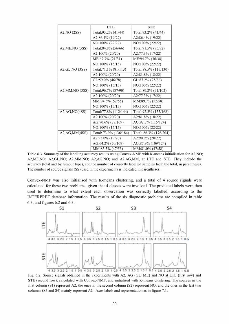
55

LTE STE A2,NO (2SS) Total:93.2% (41/44) Total:93.2% (41/44)

A2:86.4% (19/22) A2:86.4% (19/22) NO:100% (22/22) NO:100% (22/22)

A2,ME,NO (3SS) Total:84.8% (56/66) Total:91.5% (75/82) A2:100% (20/20) A2:77.3% (17/22) ME:67.7% (21/31) ME:94.7% (36/38) NO:100% (15/15) NO:100% (22/22)

A2,GL,NO (3SS) Total:71.1% (81/113) Total:88.5% (115/130) A2:100% (20/20) A2:81.8% (18/22) GL:59.0% (46/78) GL:87.2% (75/86) NO:100% (15/15) NO:100% (22/22)

A2,MM,NO (3SS) Total:96.7% (87/90) Total:89.2% (91/102) A2:100% (20/20) A2:77.3% (17/22) MM:94.5% (52/55) MM:89.7% (52/58) NO:100% (15/15) NO:100% (22/22)

A2,AG,NO(4SS) Total:77.8% (112/144) Total:92.3% (155/168) A2:100% (20/20) A2:81.8% (18/22) AG:70.6% (77/109) AG:92.7% (115/124) NO:100% (15/15) NO:100% (22/22)

A2,AG,MM(4SS) Total: 73.9% (136/184) Total: 86.3% (176/204) A2:95.0% (19/20) A2:90.9% (20/22) AG:64.2% (70/109) AG:87.9% (109/124) MM:85.5% (47/55) MM:81.0% (47/58)

Table 6.3. Summary of the labelling accuracy results using Convex-NMF with K-means initialisation for A2,NO; A2,ME,NO; A2,GL,NO; A2,MM,NO; A2,AG,NO; and A2,AG,MM, at LTE and STE. They include the accuracy (total and by tumour type), and the number of correctly labelled samples from the total, in parentheses. The number of source signals (SS) used in the experiments is indicated in parentheses. Convex-NMF was also initialised with K-means clustering, and a total of 4 source signals were calculated for these two problems, given that 4 classes were involved. The predicted labels were then used to determine to what extent each observation was correctly labelled, according to the INTERPRET database information. The results of the six diagnostic problems are compiled in table 6.3, and figures 6.2 and 6.3.

Fig. 6.2. Source signals obtained in the experiments with A2, AG (GL+ME) and NO at LTE (first row) and STE (second row), calculated with Convex-NMF, and initialised with K-means clustering. The sources in the first column (S1) represent A2, the ones in the second column (S2) represent NO, and the ones in the last two columns (S3 and S4) mainly represent AG. Axes labels and representation as in figure 7.1.

56

In the next section we use the sources in the context of supervised classification, and compare the results with equivalent classifiers, using the same settings.

6.3.2. NMF for Classification

6.3.2.1. Using Convex-NMF extracted source signals for DR prior to classification We now switch to experiments that analyse the use of Convex-NMF as a DR technique to preprocess the MRS data prior to standard classification. For this, we used the orthogonal set corresponding to the source signals obtained, and projected the data onto this basis. The SC software [99] (see chapter 3) was used to develop standard Fisher LDA classifiers, which were then evaluated through bootstrap with 1,000 repetitions. The results are shown in table 6.4. In order to compare these results with those of a traditional feature extraction method, we replicated all experiments using the SC software with PCA as data preprocessing feature extraction method (extracting a number of principal components equal to the number of source signals calculated for the corresponding NMF experiment). This was again followed by Fisher LDA classification and evaluated through bootstrap with 1,000 repetitions, as in the experiments in table 6.4. The combination of PCA+LDA has been widely used to develop MRS classifiers [24, 13, 113, 26]. The results for experiments with PCA are compiled in table 6.5. Results obtained using an independent test set are shown in table 6.6 for both FE methods: PCA and Convex-NMF.

LTE STE A2,NO (2SS) Total: 100% ± 0.0 Total: 95.5% ± 3.1

A2: 100% ± 0.0 A2: 91.2% ± 6.0 NO: 100% ± 0.0 NO: 100% ± 0.0

A2,ME,NO (3SS) Total: 92.6% ± 3.3 Total: 94.0% ± 2.6 A2: 100% ± 0.0 A2: 86.3% ± 7.4 ME: 84.1% ± 6.8 ME: 95.0% ± 3.5 NO: 100% ± 0.0 NO: 100% ± 0.0

Fig. 6.3. Source signals obtained in the experiments with A2, AG (GL+ME) and MM at LTE (first row) and STE (second row), calculated with Convex-NMF, and initialised with K-means clustering. The sources in the first column (S1) again represent A2, the ones in the second column (S2) represent MM, and the ones in the last two columns (S3 and S4) again mainly represent AG. Axes labels and representation as in previous figures.

57

A2,GL,NO (3SS) Total: 85.1% ± 3.4 Total: 91.0% ± 2.5 A2: 84.9% ± 8.5 A2: 82.5% ± 8.1 GL: 82.3% ± 4.3 GL: 90.9% ± 3.1 NO: 100% ± 0.0 NO: 100% ± 0.0

A2,MM,NO (3SS) Total: 97.7% ± 1.6 Total: 92.2% ± 2.7 A2: 94.8% ± 5.0 A2: 86.3% ± 7.7 GL: 98.2% ± 1.9 GL: 91.5% ± 3.7 NO: 100% ± 0.0 NO: 100% ± 0.0

A2,AG,NO (4SS) Total: 90.9% ± 2.4 Total: 92.3% ± 2.0 A2: 100% ± 0.0 A2: 81.9% ± 8.2 AG: 88.0% ± 3.1 AG: 92.8% ± 2.3 NO: 100% ± 0.0 NO: 100% ± 0.0

A2,AG,MM (4SS) Total: 79.4% ± 3.0 Total: 87.7% ± 2.3 A2: 94.9% ± 5.2 A2: 95.5% ± 4.6 AG: 72.5% ± 4.3 AG: 86.3% ± 3.2 MM: 87.5% ± 4.3 MM: 87.7% ± 4.3

Table 6.4. Classification results (accuracy ± SD) obtained with Fisher LDA for six diagnostic problems, from the source signals obtained by Convex-NMF, for data acquired at LTE and STE. Classifier results were validated through bootstrap. The number of source signals (SS) used in the experiments is indicated in parentheses.

LTE STE A2,NO (2PC) Total: 100% ± 0.0 Total: 93.2% ± 3.9

A2: 100% ± 0.0 A2: 86.4% ± 7.4 NO: 100% ± 0.0 NO: 100% ± 0.0

A2,ME,NO (3PC) Total: 93.8% ± 3.1 Total: 90.2% ± 3.3 A2: 100% ± 0.0 A2: 86.2% ± 7.5 ME: 86.9% ± 6.1 ME: 91.9% ± 4.4 NO: 100% ± 0.0 NO: 91.1% ± 6.0

A2,GL,NO (3PC) Total: 82.1% ± 3.6 Total: 84.4% ± 3.2 A2: 100.0% ± 0.0 A2: 81.4% ± 8.4 GL: 75.4% ± 4.9 GL: 84.6% ± 3.8 NO: 93.2% ± 6.8 NO: 86.2% ± 7.5

A2,MM,NO (3PC) Total: 95.4% ± 2.2 Total: 88.1% ± 3.2 A2: 95.0% ± 5.1 A2: 81.6% ± 8.4 MM: 94.4% ± 3.1 MM: 87.8% ± 4.2 NO: 100.0% ± 0.0 NO: 95.5% ± 4.5

A2,AG,NO (4PC) Total: 84.6% ± 3.0 Total: 86.2% ± 2.7 A2: 100% ± 0.0 A2: 72.5% ± 9.6 AG: 79.7% ± 3.9 AG: 89.5% ± 2.8 NO: 100.0% ± 0.0 NO: 81.5% ± 8.6

A2,AG,MM (4PC) Total: 80.2% ± 2.9 Total: 81.3% ± 2.7 A2: 100% ± 0.0 A2: 90.7% ± 6.4 AG: 75.9% ± 4.2 AG: 80.6% ± 3.5 NO: 81.6% ± 5.2 NO: 79.2% ± 5.3

Table 6.5. Classification results (accuracy ± SD) obtained with Fisher LDA for six diagnostic problems, from the source signals obtained by PCA, for data acquired at LTE and STE. Classifier results were validated through bootstrap. The number of principal components (PC) in the experiments is indicated in parentheses.

58

LTE, FE method:

PCA LTE, FE method:

Convex-NMF STE, FE method:

PCA STE, FE method:

Convex-NMF A2,NO

(2PC/SS)

Total:92.3%(12/13) Total:92.3%(12/13) Total:92.3%(12/13) Total:92.3%(12/13) A2: 100% (10/10) A2: 90.0%(9/10) A2: 90.0%(9/10) A2: 90.0%(9/10) NO: 66.7% (2/3) NO: 100%(3/3) NO: 100%(3/3) NO: 100%(3/3) BER: 0.17 BER: 0.05 BER: 0.05 BER: 0.05

A2,ME,NO

(3PC/SS)

Total:82.6%(19/23) Total:82.6%(19/23) Total: 73.9%(17/23) Total: 91.3%(21/23) A2: 100% (10/10) A2: 90.0% (9/10) A2: 80.0%(8/10) A2: 90.0%(9/10) ME: 70.0%(7/10) ME: 70.0%(7/10) ME: 70.0%(7/10) ME: 90.0%(9/10) NO: 66.7% (2/3) NO: 100% (3/3) NO: 66.7%(2/3) NO: 100% (3/3) BER: 0.21 BER: 0.13 BER: 0.28 BER: 0.07

A2,GL,NO

(3PC/SS)

Total: 65.1%(28/43) Total: 67.4%(29/43) Total: 76.7%(33/43) Total: 90.7%(39/43) A2: 90%(9/10) A2: 70.0%(7/10) A2: 60.0%(6/10) A2: 90.0%(9/10) GL: 53.3% (16/30) GL:63.3%(19/30) GL:80.0%(24/30) GL: 90.0%(27/30) NO: 100%(3/3) NO: 100% (3/3) NO: 100% (3/3) NO: 100% (3/3) BER: 0.19 BER: 0.22 BER: 0.20 BER: 0.07

A2,MM,NO

(3PC/SS)

Total: 81.3%(13/16) Total: 68.8%(11/16) Total: 75.0%(12/16) Total: 87.5%(14/16) A2: 80.0%(8/10) A2: 50.0%(5/10) A2: 60.0%(6/10) A2: 80.0%(8/10) MM: 66.7% (2/3) MM: 100% (3/3) MM: 100%(3/3) MM: 100% (3/3) NO: 100% (3/3) NO: 100% (3/3) NO: 100% (3/3) NO: 100% (3/3) BER: 0.18 BER: 0.17 BER: 0.13 BER: 0.07

A2,AG,NO

(4PC/SS)

Total: 64.2%(34/53) Total: 71.7%(38/53) Total: 83.0%(44/53) Total: 90.6%(48/53) A2: 90%(9/10) A2:70.0%(7/10) A2: 80.0%(8/10) A2: 90.0%(9/10) AG: 57.5%(23/40) AG: 70.0% (28/40) AG: 87.5% (35/40) AG: 90.0% (36/40) NO: 66.7% (2/3) NO: 100% (3/3) NO: 33.3%(1/3) NO: 100% (3/3) BER: 0.29 BER: 0.20 BER: 0.33 BER: 0.07

A2,AG,MM

(4PC/SS)

Total: 67.9%(36/53) Total: 64.2%(34/53) Total: 73.6%(39/53) Total: 83.0%(44/53) A2: 80% (8/10) A2: 60%(6/10) A2: 70.0%(7/10) A2: 90.0%(9/10) AG: 62.5%(25/40) AG: 62.5%(25/40) AG: 72.5% (29/40) AG: 80.0% (32/40) MM: 100% (3/3) MM: 100% (3/3) MM: 100% (3/3) MM: 100% (3/3) BER: 0.19 BER: 0.26 BER: 0.19 BER: 0.10

Table 6.6. Classification accuracies (total and by tumour type) and BER for the independent test set, using all the classification settings from tables 6.4 and 6.5, for data at LTE and STE.

6.3.2.2. Determining the most adequate number of sources One of the issues to which attention should be paid is the determination of the most appropriate number of sources for each problem. For this, we investigate the effect of varying the number of extracted sources on the classification results. For illustration, results for only one of the six previously investigated problems, namely A2,AG,MM, are presented. This problem is the most complex of those studied since it encompasses tumour type and grade, as well as extra or intra-axial origin discrimination: low grade neuroepithelial vs. high grade neuroepithelial, plus metastasis vs. low grade meningeal. Figures 6.4 and 6.5 show the different sources obtained, at LTE and STE, respectively, when we vary the number of sources. The first four rows show the results of extracting 3, 4, 5 and 6 sources, while the last rows show the percentage of contribution of each source to each tumour type, for each experiment. Tables 6.7 and 6.8 compile the classification results when varying the number of sources from 2 to 10, for the training and the independent test set, respectively; and the plots in figure 6.6 summarise the results, at LTE and STE.

59

Fig. 6.5. Sources of the problem A2,AG,MM at STE in different experiments with varying number of extracted sources. Details as in figure 7.4.

Fig. 6.4. Sources of the problem A2,AG,MM at LTE in different experiments with varying number of extracted sources. The first 4 rows show the sources corresponding to experiments in which 3, 4, 5 and 6 sources were calculated. Horizontal axis in the first four rows: frequency in ppm scale. The last row shows the percentage of contribution of each source to each tumour type, for each experiment. Horizontal axis in the last row: source signals. Vertical axes labels and representation of the sources as in previous figures.

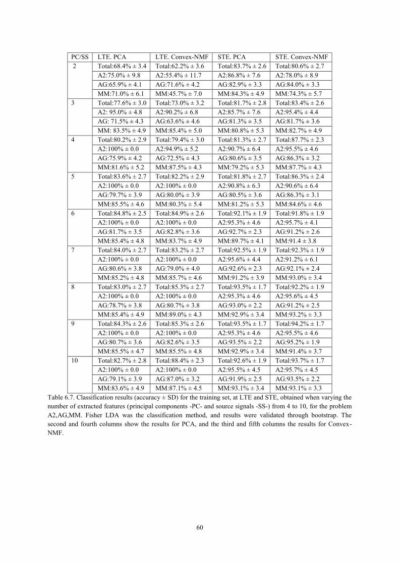
60

PC/SS LTE. PCA LTE. Convex-NMF STE. PCA STE. Convex-NMF 2 Total:68.4% ± 3.4 Total:62.2% ± 3.6 Total:83.7% ± 2.6 Total:80.6% ± 2.7

A2:75.0% ± 9.8 A2:55.4% ± 11.7 A2:86.8% ± 7.6 A2:78.0% ± 8.9 AG:65.9% ± 4.1 AG:71.6% ± 4.2 AG:82.9% ± 3.3 AG:84.0% ± 3.3 MM:71.0% ± 6.1 MM:45.7% ± 7.0 MM:84.3% ± 4.9 MM:74.3% ± 5.7

3 Total:77.6% ± 3.0 Total:73.0% ± 3.2 Total:81.7% ± 2.8 Total:83.4% ± 2.6 A2: 95.0% ± 4.8 A2:90.2% ± 6.8 A2:85.7% ± 7.6 A2:95.4% ± 4.4 AG: 71.5% ± 4.3 AG:63.6% ± 4.6 AG:81.3% ± 3.5 AG:81.7% ± 3.6 MM: 83.5% ± 4.9 MM:85.4% ± 5.0 MM:80.8% ± 5.3 MM:82.7% ± 4.9

4 Total:80.2% ± 2.9 Total:79.4% ± 3.0 Total:81.3% ± 2.7 Total:87.7% ± 2.3 A2:100% ± 0.0 A2:94.9% ± 5.2 A2:90.7% ± 6.4 A2:95.5% ± 4.6 AG:75.9% ± 4.2 AG:72.5% ± 4.3 AG:80.6% ± 3.5 AG:86.3% ± 3.2 MM:81.6% ± 5.2 MM:87.5% ± 4.3 MM:79.2% ± 5.3 MM:87.7% ± 4.3

5 Total:83.6% ± 2.7 Total:82.2% ± 2.9 Total:81.8% ± 2.7 Total:86.3% ± 2.4 A2:100% ± 0.0 A2:100% ± 0.0 A2:90.8% ± 6.3 A2:90.6% ± 6.4 AG:79.7% ± 3.9 AG:80.0% ± 3.9 AG:80.5% ± 3.6 AG:86.3% ± 3.1 MM:85.5% ± 4.6 MM:80.3% ± 5.4 MM:81.2% ± 5.3 MM:84.6% ± 4.6

6 Total:84.8% ± 2.5 Total:84.9% ± 2.6 Total:92.1% ± 1.9 Total:91.8% ± 1.9 A2:100% ± 0.0 A2:100% ± 0.0 A2:95.3% ± 4.6 A2:95.7% ± 4.1 AG:81.7% ± 3.5 AG:82.8% ± 3.6 AG:92.7% ± 2.3 AG:91.2% ± 2.6 MM:85.4% ± 4.8 MM:83.7% ± 4.9 MM:89.7% ± 4.1 MM:91.4 ± 3.8





Table 6.7. Classification results (accuracy ± SD) for the training set, at LTE and STE, obtained when varying the number of extracted features (principal components -PC- and source signals -SS-) from 4 to 10, for the problem A2,AG,MM. Fisher LDA was the classification method, and results were validated through bootstrap. The second and fourth columns show the results for PCA, and the third and fifth columns the results for Convex-NMF.

61

PC/SS LTE. PCA LTE. Convex-NMF STE. PCA STE. Convex-NMF 2 Total:54.7%(29/53) Total:54.7%(29/53) Total:73.6%(39/53) Total:71.7%(38/53)

A2:60.0%(6/10) A2:60.0%(6/10) A2:90.0%(9/10) A2:60.0%(6/10) AG:52.5% (21/40) AG:50.0%(20/40) AG:67.5%(27/40) AG:72.5% (29/40) MM:66.7% (2/3) MM:100% (3/3) MM:100% (3/3) MM:100% (3/3) BER:0.40 BER:0.30 BER:0.14 BER:0.23

3 Total: 60.4%(32/53) Total:52.8%(28/53) Total:69.8%(37/53) Total:75.5%(40/53) A2:70.0%(7/10) A2:60.0%(6/10) A2:80.0%(8/10) A2:80.0%(8/10) AG:55.0% (22/40) AG:50.0%(20/40) AG:65.0%(26/40) AG:75.0%(30/40) MM:100% (3/3) MM:66.7% (2/3) MM:100% (3/3) MM:66.7% (2/3) BER:0.25 BER:0.41 BER:0.18 BER:0.26

4 Total:67.9%(36/53) Total:64.2%(34/53) Total:73.6%(39/53) Total:83.0%(44/53) A2:80%(8/10) A2:60.0%(6/10) A2:70.0%(7/10) A2:90.0%(9/10) AG:62.5%(25/40) AG:62.5%(25/40) AG:72.5%(29/40) AG:80%(32/40) MM:100%(3/3) MM:100%(3/3) MM:100%(3/3) MM:100%(3/3) BER:0.19 BER:0.26 BER:0.19 BER:0.10

5 Total:67.9%(36/53) Total:75.5%(40/53) Total:73.6%(39/53) Total:79.2%(42/53) A2:80%(8/10) A2:70.0%(7/10) A2:70.0%(7/10) A2:80.0%(8/10) AG:62.5%(25/40) AG:75.0%(30/40) AG:72.5%(29/40) AG:77.5%(31/40) MM:100%(3/3) MM:100%(3/3) MM:100%(3/3) MM:100%(3/3) BER:0.19 BER:0.18 BER:0.19 BER:0.14

6 Total:67.9%(36/53) Total:73.6%(39/53) Total:79.2%(42/53) Total:83.0%(44/53) A2:80%(8/10) A2:70.0%(7/10) A2:70.0%(7/10) A2:90.0%(9/10) AG:62.5%(25/40) AG:72.5%(29/40) AG:82.5%(33/40) AG:82.5%(33/40) MM:100%(3/3) MM:100%(3/3) MM:66.7%(2/3) MM:66.7%(2/3) BER:0.19 BER:0.19 BER:0.27 BER:0.20

7 Total:67.9%(36/53) Total:73.6%(39/53) Total:79.2%(42/53) Total:83.0%(44/53) A2:80%(8/10) A2:70.0%(7/10) A2:70.0%(7/10) A2:90.0%(9/10) AG:62.5%(25/40) AG:72.5%(29/40) AG:82.5%(33/40) AG:82.5%(33/40) MM:100%(3/3) MM:100%(3/3) MM:66.7%(2/3) MM:66.7%(2/3) BER:0.19 BER:0.19 BER:0.27 BER:0.20

8 Total:75.5%(40/53) Total:69.8%(37/53) Total:81.1%(43/53) Total:84.9%(45/53) A2:80%(8/10) A2:70.0%(7/10) A2:80%(8/10) A2:90.0%(9/10) AG:72.5%(29/40) AG:67.5%(27/40) AG:80%(32/40) AG:85%(34/40) MM:100%(3/3) MM:100%(3/3) MM:100%(3/3) MM:66.7%(2/3) BER:0.16 BER:0.21 BER:0.13 BER:0.19

9 Total:75.5%(40/53) Total:71.7%(38/53) Total:84.9%(45/53) Total:86.8%(46/53) A2:80%(8/10) A2:70.0%(7/10) A2:90%(9/10) A2:90%(9/10) AG:72.5%(29/40) AG:70.0%(28/40) AG:82.5%(33/40) AG:87.5%(35/40) MM:100%(3/3) MM:100%(3/3) MM:100%(3/3) MM:66.7%(2/3) BER:0.16 BER:0.20 BER:0.09 BER:0.19

10 Total:73.6%(39/53) Total:69.8%(37/53) Total:86.8%(46/53) Total:84.9%(45/53) A2:80%(8/10) A2:70.0%(7/10) A2:90%(9/10) A2:90.0%(9/10) AG:70%(28/40) AG:67.5%(27/40) AG:85%(34/40) AG:85%(34/40) MM:100%(3/3) MM:100%(3/3) MM:100%(3/3) MM:66.7%(2/3) BER:0.17 BER:0.21 BER:0.08 BER:0.19

Table 6.8. Classification accuracies (total and by tumour type) and BER for the independent test set, at LTE and STE, using the corresponding classification settings from table 6.7.

62

6.4. Discussion

6.4.1. NMF as a source extraction method

The results reported in tables 6.1 and 6.2 clearly indicate that, in terms of correlation, the Convex-NMF method consistently outperforms the rest, yielding better results in nearly every experiment. The advantage of Convex-NMF is especially striking at STE (results in table 6.2). Regarding the different initialisation alternatives, correlation results do not show much dependence on the type of initialisation strategy. Random and K-means-based initialisations seem to be, overall, the best choices at both times of echo. Therefore, in all subsequent analyses, Convex-NMF with K-means initialisation was the selected method. The illustrative example of figure 6.1, in which the NMF-extracted sources are shown, reveals an effect resulting from the fact that the best correlation value between the mean of the spectra of a class and the sources is used as the indicator for selecting the source that best represents that class: for some types of NMF, this approach results in situations in which each source does not necessarily correspond univocally to a single class; sometimes, instead, a single source may encompass more than one class. This can be clearly seen in figure 6.1, where the sources calculated with the first four methods (euc, als, alspg, and alsobs) can be explained as follows: the ones in the leftmost column describe mostly the A2 and MM tumour types, respectively (the correlation values can be seen in table 6.1); the ones in the rightmost column describe the normal tissue; and the ones in the middle column have a low correlation with the three tumour types in the experiment, as evidenced if we compare them qualitatively to the mean spectra at the bottom of the figure. In stark contrast, we can also conclude from figure 6.1 (and from further results not reported here, but which are consistent with the high correlation values shown in tables 6.1 and 6.2) that Convex-NMF performs class-specific source extraction far better than the other methods studied. It is remarkable how Convex-NMF is able to extract sources that represent each class univocally. Here, A2 is

Fig. 6.6. Plot for the comparison of the classification results for the problem A2,AG,MM at both LTE and STE, when using either PCA or Convex-NMF for DR, previous to classification with Fisher LDA. Images in the left-hand side column corresponds to LTE results, while those in the right-hand side column correspond to STE results. The first row displays the accuracy of the classification for all the methods, for training and test data sets. The second row displays the BER estimates for the test data sets. Horizontal axis: number of principal components or source signals. Vertical axis: accuracy and BER, respectively.

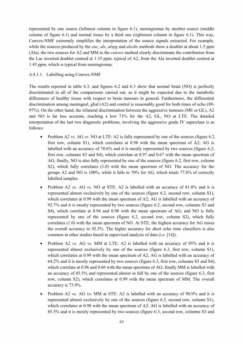
63

represented by one source (leftmost column in figure 6.1), meningiomas by another source (middle column of figure 6.1) and normal tissue by a third one (rightmost column in figure 6.1). This way, Convex-NMF extremely simplifies the interpretation of the source signals extracted. For example, while the sources produced by the euc, als, alspg and alsobs methods show a doublet at about 1.5 ppm (Ala), the two sources for A2 and MM in the convex method clearly discriminate the contribution from the Lac inverted doublet centred at 1.35 ppm, typical of A2, from the Ala inverted doublet centred at 1.45 ppm, which is typical from meningiomas.

6.4.1.1. Labelling using Convex-NMF The results reported in table 6.3, and figures 6.2 and 6.3 show that normal brain (NO) is perfectly discriminated in all of the comparisons carried out, as it might be expected due to the metabolic differences of healthy tissue with respect to brain tumours in general. Furthermore, the differential discrimination among meningeal, glial (A2) and control is reasonably good for both times of echo (89-97%). On the other hand, the trilateral discrimination between the aggressive tumours (ME or GL), A2 and NO is far less accurate, reaching a low 71% for the A2, GL, NO at LTE. The detailed interpretation of the last two diagnostic problems, involving the aggressive grade IV superclass is as follows:

Problem A2 vs. AG vs. NO at LTE: A2 is fully represented by one of the sources (figure 6.2, first row, column S1), which correlates at 0.98 with the mean spectrum of A2; AG is labelled with an accuracy of 70.6% and it is mostly represented by two sources (figure 6.2, first row, columns S3 and S4), which correlate at 0.97 and 0.67 with the mean spectrum of AG; finally, NO is also fully represented by one of the sources (figure 6.2, first row, column S2), which fully correlates (1.0) with the mean spectrum of NO. The accuracy for the groups A2 and NO is 100%, while it falls to 70% for AG, which totals 77.8% of correctly labelled samples.

Problem A2 vs. AG vs. NO at STE: A2 is labelled with an accuracy of 81.8% and it is represented almost exclusively by one of the sources (figure 6.2, second row, column S1), which correlates at 0.99 with the mean spectrum of A2; AG is labelled with an accuracy of 92.7% and it is mostly represented by two sources (figure 6.2, second row, columns S3 and S4), which correlate at 0.94 and 0.98 with the mean spectrum of AG; and NO is fully represented by one of the sources (figure 6.2, second row, column S2), which fully correlates (1.0) with the mean spectrum of NO. At STE, the highest accuracy for AG raises the overall accuracy to 92.3%. The higher accuracy for short echo time classifiers is also common in other studies based in supervised analysis of data (i.e. [14]).

Problem A2 vs. AG vs. MM at LTE: A2 is labelled with an accuracy of 95% and it is represented almost exclusively by one of the sources (figure 6.3, first row, column S1), which correlates at 0.99 with the mean spectrum of A2; AG is labelled with an accuracy of 64.2% and it is mostly represented by two sources (figure 6.3, first row, columns S3 and S4), which correlate at 0.96 and 0.66 with the mean spectrum of AG; finally MM is labelled with an accuracy of 85.5% and represented almost in full by one of the sources (figure 6.3, first row, column S2), which correlates at 0.99 with the mean spectrum of MM. The overall accuracy is 73.9%.

Problem A2 vs. AG vs. MM at STE: A2 is labelled with an accuracy of 90.9% and it is represented almost exclusively by one of the sources (figure 6.3, second row, column S1), which correlates at 0.98 with the mean spectrum of A2; AG is labelled with an accuracy of 85.5% and it is mostly represented by two sources (figure 6.3, second row, columns S3 and

64

S4), which correlate at 0.94 and 0.93 with the mean spectrum of AG; finally MM is labelled with an accuracy of 86.2% and represented almost in full by one of the sources (figure 6.3, second row, column S2), which correlates at 0.97 with the mean spectrum of MM. The overall accuracy is 86.3%. Again, at STE the accuracy for AG is higher than at LTE.

The results for the AG superclass illustrate that Convex-NMF is not always successful in extracting tumour type-specific sources. Two inherent characteristics of AG may explain this: first, AG has been artificially built using two tumour types (ME and GL) and, second, GL by itself is a rather heterogeneous type in which plenty of substructure can be found [11, 114, 115, 116, 117]. This does not preclude the interpretation of the sources. According to the signal profile and its metabolic interpretation, one of the sources representing AG (figure 6.2, first row, column S3) seems to correspond to the necrotic core (high ML) [118, 54]; while the other (figure 6.2, first row, column S4) seems to correspond to the cellular part of the tumour (high total Cho, indicating high proliferation rate [119]). Note that this dichotomy is valid for both echo times, and the two problems above, in which one source represents the cellular part while the other represents the necrotic core, and both are needed to accurately recognise SV patterns of GL or ME.

6.4.2. Convex-NMF as DR Method Prior to Classification

The comparison of the results of tables 6.4 and 6.5 reveals that at STE the classification results for the training dataset improve in all the experiments when using Convex-NMF for feature extraction instead of PCA, prior to standard supervised classification. This pattern was repeated for LTE, with the exception of the A2,AG,MM problem, which yielded a poorer result; in any case, the difference is rather small and not significant. Interestingly, the unsupervised labelling results reported in table 6.3, though worse than those of their supervised counterparts reported in table 6.4, are still comparable to those obtained with PCA and LDA in fully supervised mode (in fact, they are consistently better for STE, while worse for LTE). An independent test set was then used to further validate the robustness of the developed classifiers for data preprocessed with both FE methods: PCA and the orthogonal Convex-NMF sources. Table 6.6 contains the accuracy results (total and by tumour type), as well as the corresponding BER [26]. Again, at STE, the use of Convex-NMF orthogonal sources yields results that clearly outperform those of PCA-based classification. However, at LTE the results are more mixed: similar in the cases of A2,NO; A2,ME,NO and A2,GL,NO; better in the case of A2,AG,NO; and worse in remaining two: A2,AG,MM (with a small difference) and A2,MM,NO, with a more noticeable difference. Other studies have addressed similar problems in the existing literature, for similar data. We report next some of these results for comparative purposes, although the techniques and the evaluation criteria involved are not always the same.

In [24], as first step of a multiclass classifier for data acquired at LTE, aggressive tumours (AG) were discriminated from A2 with an accuracy of 84.7%. In our experiments, which also include the healthy tissue class, an 85.1% accuracy was achieved from the extracted sources. For the same problem, with data acquired at STE, an accuracy of 90.9% was reported in [25], to be compared with a 92.3% obtained in our study from the sources.

In [14], when classifying low-grade meningiomas (MM) vs. low-grade glial tumours (A2, plus oligodendrogliomas and oligoastrocytomas, two tumour types not analysed in our experiments) vs. high-grade aggressive tumours (AG), the reported accuracies for the

65

training set were 84.2% at LTE and 89.0% at STE, while the accuracies for an independent test set were, in turn, 69.8% and 82.5%. The results obtained in our experiments when separating A2 from AG and MM, using the sources, were 79.4% at LTE and 87.7% at STE, for training; and 64.2% at LTE and 83.0% at STE, for the independent test set.

6.4.2.1. Determining the most adequate number of sources Figures 6.4 and 6.5 show the different sources obtained, at LTE and STE, respectively, when varying the number of sources. In both figures, the first columns of sources are representing mostly the A2 type; the second columns represent mostly the MM type; and, finally, the third columns are mainly representing necrotic tissue, which should only be found in GL and ME. It is interesting to see how, when calculating 4 sources, the first 3 sources remain, while the new one seems to correspond to actively proliferating tumour (high total Cho at ca. 3.21 ppm). The bar plots for 4 sources, at both times of echo, show the extent to which sources 3 (necrotic tissue) and 4 (proliferative tumour) are representing the AG superclass. At LTE, when calculating 5 sources, the first 4 look very similar to the ones calculated in the experiment with 4 sources, while the new one seems to express part of the AG superclass, which is now in fact split into the last three sources. The non-necrotic 4th and 5th sources would show an inverted trend for total Cho (ca. 3.21 ppm) versus ML/Lac (ca. 1.3 ppm). Then, decreasing Cho would be matched by increased ML/Lac, suggesting sampling of aggressive tumour subtypes with variable proliferation rate (total Cho), with concomitant effects on the Lac and ML accumulation. At STE, when calculating 5 sources, the first four also look very similar to those obtained in the experiment with only 4 sources, but the new one is not only part of AG, but also partly of MM. Six sources at LTE already seem to be too many, given that the contribution of the last one is comparatively very small and completely unspecific. Six sources at STE also seem to be too many. In this case, the MM class is less represented by the second source, while the 5th does contribute both to AG and MM. This could have contributions from class outlier cases (atypical meningiomas), for which ML could be starting to increase. The last one could contain some artefactual bad water suppression artefact above 3.7 ppm. Up to this point, and based solely on the patterns of the sources, and the percentages of contribution of these to each class, choosing 4 or 5 sources seems to be best option, at both times of echo, to maintain the correspondence between source, or set of sources, and individual tumour types. Tables 6.7 and 6.8 compile the classification results corresponding to the varying number of sources (from 2 to 10), both for the training and the independent test set, respectively. The plots in figure 6.6 summarise these results. The leftmost column in this figure contains the results at LTE, and the rightmost column, the results at STE. Strictly in terms of classification, the use of 5 sources seems to be a good choice at LTE, given the accurate results obtained with the independent test set, and its low BER value. At STE, choosing 4 sources seems to be a good compromise, for which the accuracies for the training and the independent test set are high, while the BER for the test set stays the lowest.

6.5. Conclusions

In this chapter, we have extended the unsupervised analysis of SV 1H-MRS data from human brain tumours made in chapter 5. Convex-NMF has been shown to produce a reduced number of sources that can be confidently recognised as representing brain tumour types or healthy tissue in a way that other source extraction methods, including other NMF variants, cannot. Importantly, this result allows

66

us to produce class assignments for unlabelled spectra in fully unsupervised mode, using the mixing matrix directly as a basis for classification, with results that are comparable to those obtained in fully supervised mode. The use of the sources extracted by Convex-NMF for DR leads to simple LDA-based classifiers with independent test performances that are comparable with, and are often better than previously described strategies. In summary, the unsupervised properties of Convex-NMF place this approach one step ahead of classical label-requiring supervised methods for detection of the increasingly recognised molecular subtype heterogeneity within human brain tumours. The application of Convex-NMF in computer assisted decision support systems is expected to facilitate further improvements in the uptake of MRS-derived information by clinicians.

67

7.

Convex-NMF for the analysis of

multi-voxel MRS data

7.1. Introduction

The heterogeneity of the tissue in the brain volumes analysed by MR remains a challenge in terms of pathological area delimitation. The analysis of individual metabolite images, by itself, makes it difficult to produce a consistent segmentation between abnormal and normal tissue. This is illustrated in figure 7.1. It compiles six 10×10 colour-coded maps displaying the spatial accumulation of the principal metabolites detected by MRSI in a mouse model of brain tumour (Cho, NAA, Lac, lipids, Cr, and Ala), superimposed over the T2-W image [120].

Fig. 7.1. Peak maps of principal metabolites of one mouse (C69, see also section 7.2) harbouring a glioblastoma, scanned at 7 Tesla by PRESS-MRSI with 136 ms echo-time. MRSI data were acquired with Bruker ParaVision 4.0, and Fourier interpolated to 32×32 voxels. Line broadening adjustments and zero order phase correction were carried out. Then, the data were fed into a home-built module for MRSI post-processing, where the 4.5–0 ppm region of each spectrum was individually normalised to UL2. Each map shows the peak height in absolute values of the studied metabolite in each voxel. The white dotted lines highlight the tumoural mass. The scales reflected in the colours coding are in arbitrary units.

68

In the current chapter, a pre-clinical study was carried out using brain tumour-bearing mice. In vivo MRI and MRS were acquired from the brain and tumour tissue, along with ex vivo postmortem histology slides of the same animals. This enabled us not only to evaluate the correlation of the sources obtained with the observed spectra, but also to evaluate how accurate the calculated maps, delineating the tumour region, were with respect to a true biological correlate acquired ex vivo. This ex vivo – in vivo correlation is very difficult to achieve with human brain tumours because of the surgical protocol normally used, which loses track of the anatomical correlation with the bulk resected tissue. In summary, the aims of the experiments carried out for this chapter were to: 1) Explore the comparative ability of NMF methods to extract the constituent sources of MRSI data; 2) Investigate the possibility of creating an accurate delimitation of the tumour area, after identifying the sources that describe the tumour tissue; and 3) Generate tissue labels in a fully unsupervised mode.



The MV 1H-MRS data analysed in this thesis were seven GL261 glioblastoma multiforme (GL)-bearing mice [121]. They were scanned at 7 Tesla by PRESS-MRSI, using two different echo times: 12 ms (STE); and 136 ms (LTE). Compared to LTE, STE spectra typically show more complex patterns, including signals from metabolites with short and long T2 relaxation times. In LTE spectra, signals with short T2 will be lost, such as most lipids and macromolecules, remaining visible only spins with longer T2, i.e. small metabolites. Thus, the Lac methyl signals resonating close to the lipid methyl groups become better visible in LTE spectra. In addition, due to J-coupling effects, the methyl protons of Ala and Lac will appear inverted in LTE spectra, i.e. 180 degree phase shift compared to other visible metabolites [18]. Six of these mice, namely C69, C71, C32, C179, C233, and C234, were described in [121]. A seventh mouse, namely C278, was used in this work to increase the number of experiments. This animal was handled (tumour induction) and scanned exactly as reported for the other six. Despite the protocol in [121] consisted in acquiring time-course MRSI data during the course of hyperglycemia in mice bearing GL261 tumours, only baseline spectra of those tumours were used here, collected at euglycemia, not during hyperglycemia. Sources extracted as described in section 7.2.2 were used to create maps delimiting the tumour region. These maps were compared to the gold standard, which, in this study, is Ki67 stained sections of the post-mortem, paraffin-embedded mice brains as in [122]. Ki67 immunostaining allows the spatial determination of the proliferating population of cells in an individual tumour [123]. The proliferation index (PI), also called mitotic index, was calculated for each tumour by, first, immunohistochemical technique on paraffin-embedded slices with the Ki-67 antibody (BD Biosciences Pharmingen 550609) and, second, subsequently counting the number of positive cells per field at 40× magnification. This was achieved with the Definiens Developer XD 1.2 software* "Image Registration: MRI & Tissue Slide" package, which correlates the MRI with the corresponding Ki-67 immunostained slice with an affine transformation. The Ki67 immunostained slice that best matched the MRI slice was chosen by the pathologist following anatomical criteria. In this particular murine model, and according to the pathologist, PI>30% would correspond to a safe threshold for the tumoural region, whereas a PI≤5% would correspond to non-tumour, in agreement with similar studies (PI<12% for control) [124]. In humans, glioblastomas vary considerably in PI values, reflecting, to some extent, tumour heterogeneity [123, 125]. * http://www.definiens.com/

69

In [30] subsets of tumoural and non-tumoural regions were labelled, for each of the investigated mice, according to the following criteria: first, the spectra should not correspond to voxels at the edge of the PRESS-VOI, where signal to noise ratio (SNR) tends to be lower; and second, as in [19], they had not been collected over, or close to, the tumour borderline, to avoid as much as possible voxel ‘bleeding’ between tumour/non-tumour regions. This labelling served to compare the sources obtained with the mean spectra of tumour and non-tumoural tissue.

7.2.2. NMF for source extraction

In this study, we considered the five NMF variants (euc, als, alspg, alsobs, and convex), in the six initialisation methods (random, K-means, FCM, PCA, FastICA, and NMF itself), already described in the previous chapters. They cover a wide palette of algorithmic alternatives. As in the previous chapter, NMF is used as an unsupervised method in the sense that labelled MRSI voxels are not used to create the data model, taking advantage of the benefits that this setting offers (see chapter 6.2.4). In order to represent the data using the source signals obtained through the chosen NMF method, we propose to infer the labels of each voxel only on the basis of the mixing matrix and the calculated source signals, which will give us an idea of the extent to which each of the sources contributes to the reconstruction of each voxel. The calculation of the contribution 𝐶 of each source 𝑘 (from 𝐾 sources) to each voxel 𝑖 (from 𝑁 voxels) is estimated from the overlap between the recovered signal and the source, (as in the previous chapter, Eq. 6.1):

𝐶𝑖,𝑘 = 𝑉𝑖

𝑇𝑊𝑘𝐻𝑘,𝑖, 𝑖 = 1 … 𝑁, 𝑘 = 1 … 𝐾 (7.1)

7.2.3. Voxel labelling using the mixing matrix and the sources

For each mouse, the data matrix 𝑉 is built with the available MRSI spectra. Its dimension is 692×100 (corresponding to 692 frequencies in the spectral interval of interest and 100 voxels). All the investigated variants of the NMF method, with all considered initialisation strategies, were used to calculate the underlying source signals. The interpretation of each source was made by reference to the average spectra of the corresponding mouse regions, previously mentioned. The method was set up to calculate two source signals, under the hypothesis that one of them will represent the tumour, while the other will represent the non-tumour region. This is intended to capture the separation between the two main tissue types. After calculating the source signals and the mixing matrix, we proceeded to the calculation of the contribution 𝐶 of each source to each voxel, as described by Eq. 7.1. The vector formed with the values of 𝐶 for each voxel, for the source signal mainly representing the tumour, was used to delimit the tumour area. For this, a colour map was created using these values: red representing the highest values (i.e. the tumour), and blue, the lowest ones (i.e. non-tumour). Binary (tumour vs. non-tumour) labels for each voxel were then generated in a fully unsupervised mode. The correlations between the spectra in each voxel and each source were calculated, and the label was assigned according to the source that yielded the highest correlation. If the correlation between the spectrum of a voxel and both sources was below a threshold of 50%, then we labelled this voxel as 'undecided' (thus effectively abstaining from labelling the voxel). Assigning a colour for each source, and black for the 'undecided' voxels, we created colour maps with the labels.

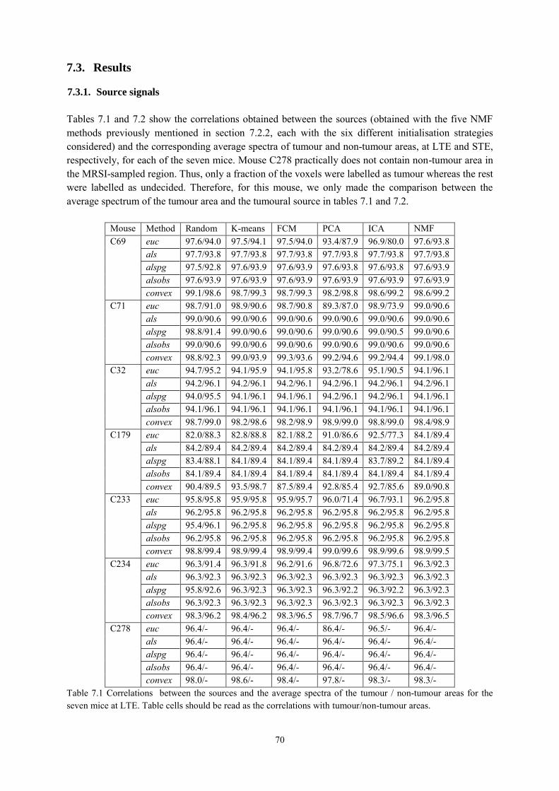
70

7.3. Results


Tables 7.1 and 7.2 show the correlations obtained between the sources (obtained with the five NMF methods previously mentioned in section 7.2.2, each with the six different initialisation strategies considered) and the corresponding average spectra of tumour and non-tumour areas, at LTE and STE, respectively, for each of the seven mice. Mouse C278 practically does not contain non-tumour area in the MRSI-sampled region. Thus, only a fraction of the voxels were labelled as tumour whereas the rest were labelled as undecided. Therefore, for this mouse, we only made the comparison between the average spectrum of the tumour area and the tumoural source in tables 7.1 and 7.2.

Mouse Method Random K-means FCM PCA ICA NMF C69 euc 97.6/94.0 97.5/94.1 97.5/94.0 93.4/87.9 96.9/80.0 97.6/93.8

als 97.7/93.8 97.7/93.8 97.7/93.8 97.7/93.8 97.7/93.8 97.7/93.8 alspg 97.5/92.8 97.6/93.9 97.6/93.9 97.6/93.8 97.6/93.8 97.6/93.9 alsobs 97.6/93.9 97.6/93.9 97.6/93.9 97.6/93.9 97.6/93.9 97.6/93.9 convex 99.1/98.6 98.7/99.3 98.7/99.3 98.2/98.8 98.6/99.2 98.6/99.2

C71 euc 98.7/91.0 98.9/90.6 98.7/90.8 89.3/87.0 98.9/73.9 99.0/90.6 als 99.0/90.6 99.0/90.6 99.0/90.6 99.0/90.6 99.0/90.6 99.0/90.6 alspg 98.8/91.4 99.0/90.6 99.0/90.6 99.0/90.6 99.0/90.5 99.0/90.6 alsobs 99.0/90.6 99.0/90.6 99.0/90.6 99.0/90.6 99.0/90.6 99.0/90.6 convex 98.8/92.3 99.0/93.9 99.3/93.6 99.2/94.6 99.2/94.4 99.1/98.0





C278 euc 96.4/- 96.4/- 96.4/- 86.4/- 96.5/- 96.4/- als 96.4/- 96.4/- 96.4/- 96.4/- 96.4/- 96.4/- alspg 96.4/- 96.4/- 96.4/- 96.4/- 96.4/- 96.4/- alsobs 96.4/- 96.4/- 96.4/- 96.4/- 96.4/- 96.4/- convex 98.0/- 98.6/- 98.4/- 97.8/- 98.3/- 98.3/-

Table 7.1 Correlations between the sources and the average spectra of the tumour / non-tumour areas for the seven mice at LTE. Table cells should be read as the correlations with tumour/non-tumour areas.

71

Mouse Method Random K-means FCM PCA ICA NMF C69 euc 95.7/98.9 96.8/99.0 96.5/99.0 91.5/81.1 80.9/99.0 96.8/99.1

als 96.7/99.1 96.7/99.1 96.7/99.1 96.7/99.1 96.7/99.1 96.7/99.1 alspg 90.2/99.0 96.8/99.1 96.8/99.1 96.9/99.1 96.2/99.1 96.8/99.1 alsobs 96.7/99.1 96.8/99.1 96.8/99.1 96.8/99.1 96.7/99.1 96.8/99.1 convex 98.1/98.3 98.5/99.2 98.6/99.7 98.3/99.6 98.3/99.7 98.4/99.8






C278 euc 95.7/- 98.7/- 98.1/- 86.5/- 89.7/- 98.1/- als 97.5/- 98.5/- 98.5/- 98.0/- 98.0/- 98.5/- alspg 89.6/- 98.5/- 98.5/- 97.2/- 97.2/- 98.4/- alsobs 98.0/- 98.5/- 98.5/- 97.6/- 97.7/- 98.5/- convex 98.8/- 99.8/- 99.6/- 99.2/- 99.5/- 99.4/-

Table 7.2. Correlations between the sources and the average spectra of the tumour / non-tumour areas for the seven mice at STE. Table cells should be read as in table 7.1. Convex-NMF yields, overall and consistently, the best correlation results. The results are also fairly insensitive to the initialisation strategy. The source signals calculated in the experiments carried out with all mice at LTE and STE, using Convex-NMF with K-means initialisation, are displayed in figure 7.2. In order to visualize the similarities and differences of the calculated sources with respect to the average spectra of areas labelled by the expert as tumour and non-tumour, we superimposed the calculated sources to the average spectra, and to the set of all labelled spectra, as shown in figure 7.2. The sources in the first and third columns have a clear pathological profile, as expressed by the presence of high Cho, Lac and ML peaks and low or no NAA [121, 126]. Instead, the sources in the second and fourth columns mostly represent non-tumour tissue.

72

Figure 7.3 shows detailed correlation (top row) and RMSE (bottom row) results for all the analysed mice at both echo times, where sources were obtained using Convex-NMF with K-means initialisation. These results include both tumour (darker bars) and non-tumour tissue (lighter bars).

A B

Fig. 7.2. Sources obtained for the seven mice at A) LTE and B) STE. The calculated sources are shown in black colour, the average spectra in red, and all the labelled spectra in gray. The sources in the left column represent the tumour, and the ones in the right column mainly represent non-tumoral tissue. Frequencies in the horizontal axis are measured in ppm.

73

7.3.2. Tumour delimitation

Figure 7.4 shows the T2-W image for one of the studied mice (C69), together with the respective histology superimposed, using monoclonal antibody against Ki67, and Ki67 PI maps for voxels with PI<5% and PI>30%. The yellow squares delimit the VOI region. The VOI of the same mouse is further detailed in figure 7.5, enlarged and overlaid with the 10×10 MRSI spectral matrix at LTE. The areas delimited by red and blue lines correspond to characteristic tumour and non-tumour labels, respectively, labelled as in [30]. These labels will be later on in the study (section 7.3.3) referred to as "original". The yellow dotted line in figure 7.5 delineates the "anomaly region" as judged from the mass shown in the T2-W image.

We illustrate the tumour delimitation capabilities of the method proposed in this chapter on figure 7.6. This figure shows the colour maps generated for the VOI regions of mouse C69 at LTE and STE. The first row shows the 10×10 grid of voxels, with the corresponding colour according to the values of 𝐶 calculated from Eq. 7.1 for the source representing the tumour in each voxel. This is then superimposed over the T2-W image to verify the high correspondence between the area of the tumour in both images (the colour map and the T2-W). The maps displayed in the bottom row are created with a linear interpolation of the maps in the top row, also superimposed over the corresponding T2-W image.

Fig. 7.4. From left to right: T2-W image; Ki67 immunostained digitised slide; Ki67 map with PI<5%; and Ki67 map with PI>30%, of mouse C69, bearing a GL261 glioblastoma tumour. The last two maps are superimposed on the corresponding reference T2-W image. Colour columns at right show PI scale (percentage).

Fig. 7.3. Correlations (top row) and errors (bottom row) between the source signals and the average spectra of the labelled areas (as measured by RMSE). Dark gray bars, tumours; light gray bars, non-tumour tissue.

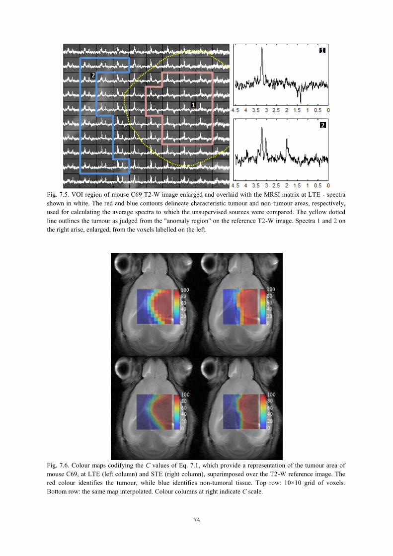
74

Fig. 7.6. Colour maps codifying the C values of Eq. 7.1, which provide a representation of the tumour area of mouse C69, at LTE (left column) and STE (right column), superimposed over the T2-W reference image. The red colour identifies the tumour, while blue identifies non-tumoral tissue. Top row: 10×10 grid of voxels. Bottom row: the same map interpolated. Colour columns at right indicate C scale.

Fig. 7.5. VOI region of mouse C69 T2-W image enlarged and overlaid with the MRSI matrix at LTE - spectra shown in white. The red and blue contours delineate characteristic tumour and non-tumour areas, respectively, used for calculating the average spectra to which the unsupervised sources were compared. The yellow dotted line outlines the tumour as judged from the "anomaly region" on the reference T2-W image. Spectra 1 and 2 on the right arise, enlarged, from the voxels labelled on the left.

75

7.3.3. Voxel labelling

As described in section 7.2.5, the values in C calculated from Eq. 7.1 were used to generate a binary label in a fully unsupervised mode. The colour maps with the labels generated for mouse C69 at LTE and STE are shown in figure 7.7. As in figure 7.6, we superimposed these maps to T2-W images, to verify the correspondence between the tumour areas described by both imaging approaches.

There is a single black voxel in figure 7.7 (colour map with labels generated for C69 at LTE). This voxel is labelled as 'undecided', indicating that the correlations of the sources with the original spectrum of this voxel (same position in figure 7.5: poor SNR), are under the 50% threshold. To determine the extent to which the obtained colour maps with labels are related to the Ki67 maps, we calculated the accuracy of the first compared to Ki67 PI maps. For this, we considered PI>30% as "surely" tumoural region, and PI≤5% as non-tumour, according to the opinion of the expert pathologist. In order to countercheck the validity of the results, a manual sampling and count of 0.1 mm2 squares along the vertical and horizontal axes of the tumour (figure 7.8) revealed that the bottom (caudal) edge of the tumour, even if clearly delimited, was surrounded by areas with a PI of 13% due to proliferating glial cells in the Cornu Ammonis (CA) of the hippocampus. As shown for mouse C69, this area was adjacent to the caudal side of the tumour mass, whereas the top (rostral), right and left immediately adjacent to the tumour areas had a PI of 0, 5.4, and 3.3% respectively. These results would agree with the spread of the source of the tumoural area observed outside the caudal T2-W anomaly region (figure 7.6 and 7.7). The mean of samplings performed inside the tumour mass yielded a PI of 73.9% and cellularity of 3647 cells/mm2 (2251 proliferating cells/mm2), consistent with a similar study (ca. 2000 proliferating cells/mm2), reported in [127].

Fig. 7.7. Colour maps with the labels generated for mouse C69, at LTE (left) and STE (right), superimposed to the T2-W reference image. The red colour identifies tumour, blue identifies non-tumour, and black represents 'undecided'. The colour intensities shown in the scale bar at right correspond to the correlation values between the spectra of the voxels and their representing source.

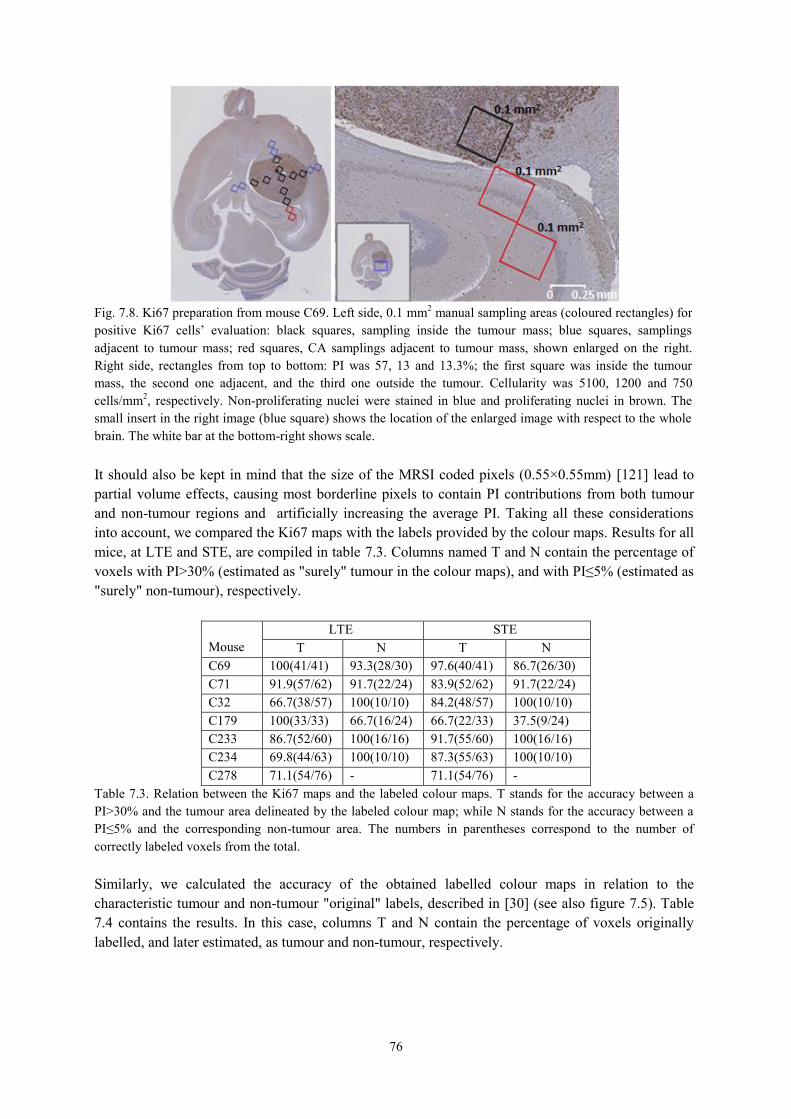
76

It should also be kept in mind that the size of the MRSI coded pixels (0.55×0.55mm) [121] lead to partial volume effects, causing most borderline pixels to contain PI contributions from both tumour and non-tumour regions and artificially increasing the average PI. Taking all these considerations into account, we compared the Ki67 maps with the labels provided by the colour maps. Results for all mice, at LTE and STE, are compiled in table 7.3. Columns named T and N contain the percentage of voxels with PI>30% (estimated as "surely" tumour in the colour maps), and with PI≤5% (estimated as "surely" non-tumour), respectively.

Mouse

LTE STE T N T N

C69 100(41/41) 93.3(28/30) 97.6(40/41) 86.7(26/30) C71 91.9(57/62) 91.7(22/24) 83.9(52/62) 91.7(22/24) C32 66.7(38/57) 100(10/10) 84.2(48/57) 100(10/10) C179 100(33/33) 66.7(16/24) 66.7(22/33) 37.5(9/24) C233 86.7(52/60) 100(16/16) 91.7(55/60) 100(16/16) C234 69.8(44/63) 100(10/10) 87.3(55/63) 100(10/10) C278 71.1(54/76) - 71.1(54/76) -

Table 7.3. Relation between the Ki67 maps and the labeled colour maps. T stands for the accuracy between a PI>30% and the tumour area delineated by the labeled colour map; while N stands for the accuracy between a PI≤5% and the corresponding non-tumour area. The numbers in parentheses correspond to the number of correctly labeled voxels from the total. Similarly, we calculated the accuracy of the obtained labelled colour maps in relation to the characteristic tumour and non-tumour "original" labels, described in [30] (see also figure 7.5). Table 7.4 contains the results. In this case, columns T and N contain the percentage of voxels originally labelled, and later estimated, as tumour and non-tumour, respectively.

Fig. 7.8. Ki67 preparation from mouse C69. Left side, 0.1 mm2 manual sampling areas (coloured rectangles) for positive Ki67 cells’ evaluation: black squares, sampling inside the tumour mass; blue squares, samplings adjacent to tumour mass; red squares, CA samplings adjacent to tumour mass, shown enlarged on the right. Right side, rectangles from top to bottom: PI was 57, 13 and 13.3%; the first square was inside the tumour mass, the second one adjacent, and the third one outside the tumour. Cellularity was 5100, 1200 and 750 cells/mm2, respectively. Non-proliferating nuclei were stained in blue and proliferating nuclei in brown. The small insert in the right image (blue square) shows the location of the enlarged image with respect to the whole brain. The white bar at the bottom-right shows scale.

77

Mouse

LTE STE T N T N

C69 100(17/17) 100(14/14) 100(17/17) 100(14/14) C71 100(26/26) 100(7/7) 100(26/26) 100(7/7) C32 91.7(22/24) 100(10/10) 100(24/24) 100(10/10) C179 100(9/9) 100(9/9) 88.9(8/9) 66.7(6/9) C233 100(29/29) 100(12/12) 100(29/29) 100(12/12) C234 84.4(27/32) 100(5/5) 100(32/32) 100(5/5) C278 87.5(35/40) - 92.5(37/40) -

Table 7.4. Relationship between the original labels and the labelled colour maps. T stands for the accuracy between the original tumour labels (as in figure 7.5) and the tumour area delineated by the labelled colour maps; while N stands for the accuracy between the non-tumour labels and the corresponding non-tumour area. The numbers in parentheses correspond to the number of correctly labelled voxels from the total. Table 7.5 compiles the sensitivity (true positive rate, 𝑇𝑃 (𝑇𝑃 + 𝐹𝑁)⁄ , where true positive (𝑇𝑃) cases are tumour voxels correctly labelled as tumours, and false negative (𝐹𝑁) cases are non-tumour voxels labelled as tumours) and specificity (true negative rate, 𝑇𝑁 (𝑇𝑁 + 𝐹𝑃)⁄ , where true negative (𝑇𝑁) cases are non-tumour voxels correctly identified as non-tumours, and false positive (𝐹𝑃) cases are tumour voxels labelled as non-tumours) of the obtained labelled colour maps. An interesting result is that comparison with Ki67 maps (figure 7.4) yields in all cases lower sensitivity and specificity than comparison with the "original" manually-labelled voxels (figure 7.5). This is probably caused by the already mentioned effect of incorporating borderline pixels in the calculation when analysing images, while the "original" labelled images take into account less borderline pixels between tumour and non-tumour tissue. Echo time does not appear to affect the results, neither when comparing with the Ki67 maps nor when comparing with the "original" labels. Figure 7.9 summarises the information for the remaining 6 mice (C71, C32, C179, C233, C234, and C278). The first four rows contain the known information about these mice, used in here to assess the accuracy of the results obtained, compiled in the last four rows. Concerning the non-tumour area of mouse C179, data shown in figures 7.8, 7.9 and 7.10, and tables 7.3 and 7.4, suggests that the sub-optimal agreement of source-derived maps (especially at STE) and Ki67 maps, may be originated from having two masses, instead of just one. This will produce a higher percentage of borderline voxels and, accordingly, a higher partial volume effect.

Mouse

LTE STE Ki67 Original Ki67 Original

C69 1.00/0.93 1.00/1.00 0.98/0.87 1.00/1.00 C71 0.92/0.92 1.00/1.00 0.84/0.92 1.00/1.00 C32 0.67/0.46 0.92/1.00 0.84/1.00 1.00/1.00 C179 1.00/0.50 1.00/1.00 0.67/0.38 0.89/0.86 C233 0.87/0.48 1.00/1.00 0.92/1.00 1.00/1.00 C234 0.70/0.47 0.84/1.00 0.87/1.00 1.00/1.00 C278 0.71/- 0.88/- 0.71/- 0.93/-

Table 7.5. Sensitivity and specificity (sensitivity/specificity) calculated for the labelled colour maps with respect to the Ki67 maps (columns named as Ki67, computed as in table 7.3), and the original labels provided (columns named as 'Original', computed as in table 7.4), for each mouse, at LTE and STE.

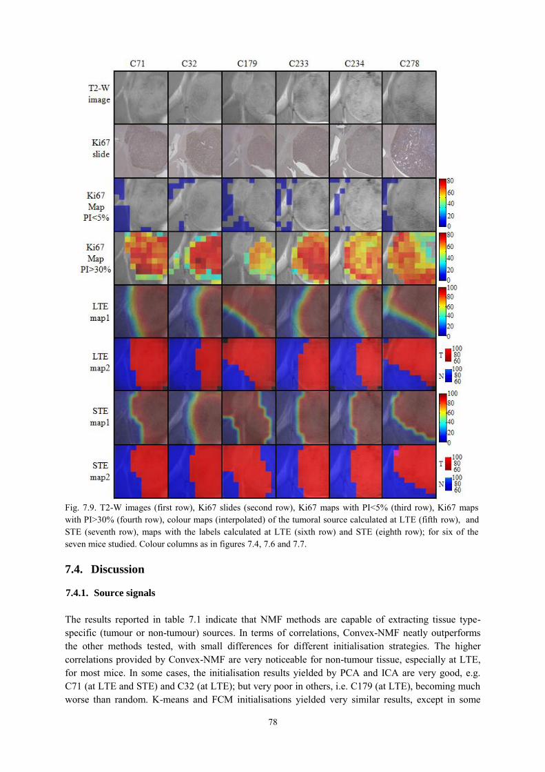
78

7.4. Discussion


The results reported in table 7.1 indicate that NMF methods are capable of extracting tissue type-specific (tumour or non-tumour) sources. In terms of correlations, Convex-NMF neatly outperforms the other methods tested, with small differences for different initialisation strategies. The higher correlations provided by Convex-NMF are very noticeable for non-tumour tissue, especially at LTE, for most mice. In some cases, the initialisation results yielded by PCA and ICA are very good, e.g. C71 (at LTE and STE) and C32 (at LTE); but very poor in others, i.e. C179 (at LTE), becoming much worse than random. K-means and FCM initialisations yielded very similar results, except in some

Fig. 7.9. T2-W images (first row), Ki67 slides (second row), Ki67 maps with PI<5% (third row), Ki67 maps with PI>30% (fourth row), colour maps (interpolated) of the tumoral source calculated at LTE (fifth row), and STE (seventh row), maps with the labels calculated at LTE (sixth row) and STE (eighth row); for six of the seven mice studied. Colour columns as in figures 7.4, 7.6 and 7.7.

79

cases in which FCM performed worse, i.e. C179 (at LTE and STE). The combination of Convex-NMF and K-means initialisation was the most stable of all, providing very good correlation results. In a previous study [110], where we assessed the abilities of two variants of ICA [35, 85], namely JADE [86] and FastICA [87], to identify the constituent tissue types in SV MRS, ICA showed no advantages over NMF methods. With respect to the acquisition conditions, although the source at LTE outperforms the source at STE for delineating normal tissue, both LTE and STE source maps perform well, one or the other with higher accuracy depending on the specific mouse studied (table 7.3). The results in figure 7.2 support our initial assumption that the two main sources obtained by Convex-NMF correspond to tumour and non-tumour tissues. GL usually shows strong ML MRS signals (at ca. 1.3ppm), most evident at STE [54] (see figure 7.2.B, left column). Normal brain tissue is usually characterised by a clear NAA peak at 2.02ppm with similar height to Cr (3.03ppm) and Cho-containing compound (3.21 ppm) peaks [126]. In the tumour area, the Cr peak height decreases, while the total Cho peak increases. Lactate (1.3ppm) resonances appear inverted at LTE (see figure 7.2.A, left column) but overlap lipid signals at STE (see figure 7.2.B, left column). Of all the mice studied, C179, with two abnormal masses, yielded the worst results. This was seen particularly at STE, and at LTE for the non-tumoural area. The smaller mass had, specifically, proliferation values between 5 and 30%. A detailed analysis of the original image (figure 7.9, third column, second row) shows a transition area of proliferating cells, between the big and the small mass (figure 7.10). Despite this particular case, the remaining six mice studied showed a clearly circumscribed tumoural mass, essentially with no infiltration outside the tumour. Only mouse C69, already discussed, had a tumoural source that extended over MRI-normal areas of the brain in its caudal part (figure 7.8), which corresponded to PI=13%. Ki67 positive cells detected outside the tumour mass were not tumoural but glial cells (morphologically detected by the expert pathologist). In this respect, it has previously been described that proliferative reactive astrocytes (astrogliosis) are attracted to brain tumours [128]. Anatomically, this was observed in the hippocampus region, which is known to contain proliferating neural stem cells (NSC) [129]. Indeed, increased proliferation of NSC and tropism towards GL261 glioblastomas has been demonstrated [130].

80

7.4.2. Tumour delimitation

Previous work [50] applying NMF to MRSI data of pathological states, either on acute or chronic phases, yielded a recovered abnormal image beyond the regions of abnormal signal intensity on T2-W Fluid Attenuated Inversion Recovery (FLAIR) images (T2-W with flowing liquid attenuation) [131]. While correctly mapping the abnormalities, our approach provides a far more precise delineation of the abnormal area. In addition, since we applied Convex-NMF to a preclinical model rather than to human patients, there is an authentic biological correlate of the true proliferative tumour area, as shown by the histopathology co-localised images. Our results match well the tumoural area, and no area beyond the proliferating abnormal area is rendered by our proposed method, even in those two cases already discussed in the previous section (7.4.1). Other, perhaps simpler, approaches would also be feasible for brain tumours, such as the CNI index (essentially a Cho/NAA ratio normalised to the normal contralateral brain ratio) [47]. In the latter work, cancer was predicted with 86% specificity and 90% sensitivity using a CNI threshold of 2.5, but, due to technical limitations, only selected target regions could be evaluated - this was not the case in our preclinical study. Specificity, when considering selected target regions (original labels), was 100% for LTE maps; sensitivity was 100% for 4/7 mice and between 84-92% in the remaining 3/7 mice (table 7.5). Finally, the hyperpolarised Lac/pyruvate ratio may also provide a handle for tumour/brain discrimination, both in developing tumour and upon therapy response [132, 133], although the low Lac signal detectable in normal brain tissue may cause difficulties in defining the border between normal and abnormal tissue.

7.4.3. Voxel labelling

The red area obtained for both colour maps in figure 7.7 corresponds to the tumoural area previously delimited and to the true proliferative tumour area, as shown by the Ki67 images. This similarity has been achieved using our proposed method to generate colour maps, with voxel labelling, which is fully unsupervised. Previous approaches for brain tumour segmentation based on MRS labelling, such as

Fig. 7.10. Ki67 preparation from mouse C179. The connecting region between the two tumour masses is shown enlarged, displaying three 0.1 mm2 areas manually sampled. From top (smaller mass) to bottom (main mass), PI: 40%, 21.5%, 24.5%, and 62.7%. White bar at bottom-left corner shows the scale. Insert at the bottom left corner shows the location of the enlarged image (blue rectangle) with respect to the whole brain.

81

[134], are all supervised. This unsupervised approach would allow us to provide a labelling prediction independent of the availability of a labelled data set. While all existing unsupervised strategies are based on MRI, for human brain tumours the area of metabolic abnormality is usually much larger than the area delimited by conventional MRI [135]. This may lead, e.g., to inaccuracies in the prediction of target volumes for radiotherapy.

7.5. Conclusions

In this chapter, we have extended the investigations on the use of NMF for the analysis of SV 1H-MRS presented in the previous chapters to the multi-voxel context. We have provided experimental evidence supporting that a very accurate delimitation can be achieved through the application of blind source extraction techniques to MV 1H-MRS data. More specifically, we have proposed and tested a fully unsupervised methodology that uses Convex-NMF source extraction to accurately delimitate the tumour region. This method was successfully benchmarked against alternative NMF methodologies. The accuracy of tissue delineation was confirmed by comparison with the gold standard of tissue assignment, by direct histopathological measurements in the tumoural region.

83

8.

Conclusions

8.1. General conclusions

The first result of this thesis corresponds to the need for tools that allowed a rapid development of multiple classifiers for the already existing MRS databases, as well as to test hypotheses that might surface during the process of data collection. For this, we developed a software tool, aimed to be used by expert spectroscopists, that facilitates the development of classifiers for the analysis of MRS data, for a large group of tumour types. That should allow them to concentrate on the interpretation of the results, without requiring a specialised mathematical expertise for testing their hypotheses. This tool also made it possible for us to reproduce previously published MRS-based classifiers, and test new hypotheses that led to new publications. Later on, we pursued new alternatives to improve the discrimination of some tumour types and subtypes that were very difficult to discriminate, extending the palette of data analysis methods. To achieve this, our first approach led us to define a novel FE method that, even if providing interesting and interpretable results, was still limited by its incapacity to provide adequate inference for previously unseen data, thus thwarting its practical application. By changing the focus of analysis to BSS techniques, we identified, after an exhaustive evaluation, the spectral decomposition variant that best suits the analysis of SV MRS data, namely Convex-NMF, and showed its ability to discriminate between healthy tissue, necrosis, and actively proliferating tumour. On the basis of these findings, we were able to provide an unsupervised alternative to improve the discrimination between tumour types and subtypes, placing this approach one step ahead of classical label-requiring supervised methods for detection of the increasingly recognised molecular subtype heterogeneity within human brain tumours. This also allowed us to accurately tackle one of the main sources of uncertainty in the clinical management of brain tumours, which is the difficulty of appropriately delimiting the pathological area. We provided evidence supporting that very accurate delimitation can be achieved through the application of Convex-NMF to MV MRS in combination with tumour imaging.

8.2. Summary of contributions

The contributions of this thesis can be summarised as follows.

A software tool for classifier development, tailored to the specific needs of MRS data analysis. It enabled the reproduction of previously published MRS-based classifiers, as well as hypotheses testing.

84

A novel FE method, SPE, whose performance is comparable to PCA, its most commonly used counterpart in MRS data analysis, while improving on the interpretability of the results.

The detailed assessment of which BSS technique, ICA or NMF, is most appropriate for the analysis of SV MRS data and most robust in the presence of noise.

The identification of the NMF variant, and its initialisation condition, that best suits the analysis of SV and MV data, namely Convex-NMF.

The evaluation of the ability of Convex-NMF to discriminate between healthy tissue, necrosis, and actively proliferating tumour.

The use of the extracted sources for DR, leading to simple classifiers with independent test performances that are comparable with, and are often better than, previously described strategies.

The mechanisms to produce, in a fully unsupervised way, accurate maps delineating the pathological area of the brain.

8.3. Future directions

This thesis creates some openings for future lines of research. We consider here two of those potential avenues of investigation: a semi-supervised approach for the extraction of relevant sources; and a hierarchical Bayesian approach for MRS multi-modal analysis.

8.3.1. Semi-supervised approach for extracting relevant sources

Providing unsupervised techniques to create a model of the analysed data –that is, without prior information regarding tumour type and grade– has been one of the central goals of the current thesis. This approach should minimise the negative effect of possible mislabelled cases or voxels, which could introduce unwanted variation in the analysis. However, some instability in the classification may be found, arising from intrinsic mixing in data space, especially for challenging differential assignments such as the discrimination of low astrocytic tumours from high grade and from metastatic growths. This limitation occurs because the proposed methods are fully unsupervised. For this reason, we plan to investigate in the future the possibility of adding some prior knowledge to the data currently available, turning our analysis into a semi-supervised one. To achieve this, we propose a three stage approach: first, to define a Fisher information metric; second, to approximate the empirical data distribution with a Euclidean projective space onto which NMF can be applied; and third, to apply Convex-NMF for the decomposition of the data. Preliminary results with synthetic data models of real-world high-dimensional data, reported in [136], indicate that the classification accuracy of the method is encouraging for challenging problems, while retaining interpretability. One of the future directions of this thesis is to extend this preliminary semi-supervised approach investigation to the analysis of SV MRS data from humans; and MV MRSI data from pre-clinical investigations involving animal models. We expect to increase the accuracies calculated in chapters 5 and 6, as well as to improve the delineation of the tumoural zone in the colour maps obtained in chapter 7.

85

8.3.2. Hierarchical Bayesian approach for multi-modal analysis

The radiologic evaluation of patients with abnormal brain masses includes the application, evaluation and integration of results from different MR techniques. In this thesis we considered two of them, MRS and MRSI; partially supporting the results of the latter by reference to the abnormal regions suggested by T2-W images. Nevertheless, other modalities used in the current radiological practice are able to provide useful insights. Examples of these are T1-W, T2-W, FLAIR, diffusion-weighted imaging (DWI), perfusion-weighted imaging (PWI), contrast enhanced images, apparent diffusion coefficient (ADC) maps, to name a few. The provision of a framework in which several of these modalities could be integrated, thereby improving the diagnosis of the pathological area, is of great interest. A possible future direction of this thesis would entail the development of a new methodology that integrated information from some of the different MR modalities mentioned above in a coherent and computationally efficient Bayesian framework, enabling robust brain tumour classification. Hierarchical Bayesian modelling, which has achieved notoriety in recent years, is considered to be specifically well suited to deal with this kind of problems. This paradigm allows considering a much richer class of models that should be able to capture better the statistical understanding of the problem. The basic idea in a hierarchical Bayesian model is to use priors that depend on other parameters not included in the likelihood. These parameters themselves will require priors, which might depend on new parameters. Eventually, the process terminates when new parameters are no further introduced. For the problem addressed here, given that there is a need of modelling multiple data types, each data source needs be modelled using the appropriate prior probability distribution, regarding its data type. Also, a new implementation of Convex-NMF in a Bayesian framework would facilitate data fusion in a natural way.

87

References

[1] World Health Organization. (2012, February) Cancer. Fact sheet N°297. [Online]. Available: http://www.who.int/mediacentre/factsheets/fs297/en/index.html

[2] B. W. Stewart and P. Kleihues, World Cancer Report 2008. International Agency for Research on Cancer (IARC), 2008.

[3] R. G. Lee P L, Gonzalez, “Magnetic resonance spectroscopy of brain tumors,” Current Opinion in Oncology, vol. 12, no. 3, pp. 199–204, 2000.

[4] M. Julià-Sapé, D. Acosta, C. Majós, A. Moreno-Torres, P. Wesseling, J. J. Acebes, J. R. Griffiths, and C. Arús, “Comparison between neuroimaging classifications and histopathological diagnoses using an international multicenter brain tumor magnetic resonance imaging database,” Journal of Neurosurgery, vol. 105, no. 1, pp. 6–14, 2006.

[5] N. A. Sibtain, F. A. Howe, and D. E. Saunders, “The clinical value of proton magnetic resonance spectroscopy in adult brain tumours,” Clinical Radiology, vol. 62, no. 2, pp. 109–119, 2007.

[6] J. Luts, A. Heerschap, J. A. K. Suykens, and S. Van Huffel, “A combined MRI and MRSI based multiclass system for brain tumour recognition using LS-SVMs with class probabilities and feature selection,” Artificial Intelligence in Medicine, vol. 40, no. 2, pp. 87–102, 2007.

[7] P. J. G. Lisboa, A. Vellido, R. Tagliaferri, F. Napolitano, M. Ceccarelli, J. D. Martin-Guerrero, and E. Biganzoli, “Data mining in cancer research,” IEEE Computational Intelligence Magazine, vol. 5, no. 1, pp. 14–18, 2010.

[8] H. Bruhn, J. Frahm, M. L. Gyngell, K. D. Merboldt, W. Hänicke, R. Sauter, and C. Hamburger, “Noninvasive differentiation of tumors with use of localized H-1 MR spectroscopy in vivo: initial experience in patients with cerebral tumors,” Radiology, vol. 172, no. 2, pp. 541–548, 1989.

[9] W. Negendank, “Studies of human tumors by MRS: a review,” NMR in Biomedicine, vol. 5, no. 5, pp. 303–324, 1992.

[10] W. El-Deredy, “Pattern recognition approaches in biomedical and clinical magnetic resonance spectroscopy: a review,” NMR in Biomedicine, vol. 10, no. 3, pp. 99–124, 1997.

[11] A. R. Tate, J. R. Griffiths, I. Martínez-Pérez, A. Moreno, I. Barba, M. E. Cabañas, D. Watson, J. Alonso, F. Bartumeus, F. Isamat, I. Ferrer, F. Vila, E. Ferrer, A. Capdevila, and C. Arús, “Towards a method for automated classification of 1H MRS spectra from brain tumours,” NMR in Biomedicine, vol. 11, no. 4-5, pp. 177–191, 1998.

[12] INTERPRET project (2000/01/01 - 2002/12/31). International Network for Pattern Recognition of Tumours Using Magnetic Resonance. IST-1999-10310. [Online]. Available: http://-azizu.uab.es/interpret

[13] A. R. Tate, J. Underwood, D. M. Acosta, M. Julià-Sapé, C. Majós, A. Moreno-Torres, F. A. Howe, M. van der Graaf, V. Lefournier, M. M. Murphy, A. Loosemore, C. Ladroue, P. Wesseling, J. Luc Bosson, M. E. Cabañas, A. W. Simonetti, W. Gajewicz, J. Calvar, A. Capdevila, P. R. Wilkins, B. A. Bell, C. Rémy, A. Heerschap, D. Watson, J. R. Griffiths, and C. Arús, “Development of a decision support system for diagnosis and grading of brain tumours

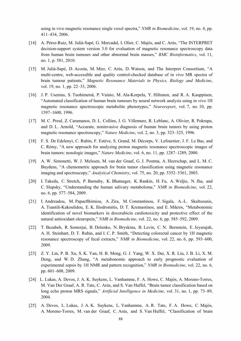
88

using in vivo magnetic resonance single voxel spectra,” NMR in Biomedicine, vol. 19, no. 4, pp. 411–434, 2006.

[14] A. Pérez-Ruiz, M. Julià-Sapé, G. Mercadal, I. Olier, C. Majós, and C. Arús, “The INTERPRET decision-support system version 3.0 for evaluation of magnetic resonance spectroscopy data from human brain tumours and other abnormal brain masses,” BMC Bioinformatics, vol. 11, no. 1, p. 581, 2010.

[15] M. Julià-Sapé, D. Acosta, M. Mier, C. Arús, D. Watson, and The Interpret Consortium, “A multi-centre, web-accessible and quality control-checked database of in vivo MR spectra of brain tumour patients,” Magnetic Resonance Materials in Physics, Biology and Medicine, vol. 19, no. 1, pp. 22–33, 2006.

[16] J. P. Usenius, S. Tuohimetsä, P. Vainio, M. Ala-Korpela, Y. Hiltunen, and R. A. Kauppinen, “Automated classification of human brain tumours by neural network analysis using in vivo 1H magnetic resonance spectroscopic metabolite phenotypes,” Neuroreport, vol. 7, no. 10, pp. 1597–1600, 1996.

[17] M. C. Preul, Z. Caramanos, D. L. Collins, J. G. Villemure, R. Leblanc, A. Olivier, R. Pokrupa, and D. L. Arnold, “Accurate, noninvasive diagnosis of human brain tumors by using proton magnetic resonance spectroscopy,” Nature Medicine, vol. 2, no. 3, pp. 323–325, 1996.

[18] F. S. De Edelenyi, C. Rubin, F. Estève, S. Grand, M. Décorps, V. Lefournier, J. F. Le Bas, and C. Rémy, “A new approach for analyzing proton magnetic resonance spectroscopic images of brain tumors: nosologic images,” Nature Medicine, vol. 6, no. 11, pp. 1287–1289, 2000.

[19] A. W. Simonetti, W. J. Melssen, M. van der Graaf, G. J. Postma, A. Heerschap, and L. M. C. Buydens, “A chemometric approach for brain tumor classification using magnetic resonance imaging and spectroscopy,” Analytical Chemistry, vol. 75, no. 20, pp. 5352–5361, 2003.

[20] I. Takeda, C. Stretch, P. Barnaby, K. Bhatnager, K. Rankin, H. Fu, A. Weljie, N. Jha, and C. Slupsky, “Understanding the human salivary metabolome,” NMR in Biomedicine, vol. 22, no. 6, pp. 577–584, 2009.

[21] I. Andreadou, M. Papaefthimiou, A. Zira, M. Constantinou, F. Sigala, A.-L. Skaltsounis, A. Tsantili-Kakoulidou, E. K. Iliodromitis, D. T. Kremastinos, and E. Mikros, “Metabonomic identification of novel biomarkers in doxorubicin cardiotoxicity and protective effect of the natural antioxidant oleuropein,” NMR in Biomedicine, vol. 22, no. 6, pp. 585–592, 2009.

[22] T. Bezabeh, R. Somorjai, B. Dolenko, N. Bryskina, B. Levin, C. N. Bernstein, E. Jeyarajah, A. H. Steinhart, D. T. Rubin, and I. C. P. Smith, “Detecting colorectal cancer by 1H magnetic resonance spectroscopy of fecal extracts,” NMR in Biomedicine, vol. 22, no. 6, pp. 593–600, 2009.

[23] Z. Y. Lin, P. B. Xu, S. K. Yan, H. B. Meng, G. J. Yang, W. X. Dai, X. R. Liu, J. B. Li, X. M. Deng, and W. D. Zhang, “A metabonomic approach to early prognostic evaluation of experimental sepsis by 1H NMR and pattern recognition,” NMR in Biomedicine, vol. 22, no. 6, pp. 601–608, 2009.

[24] L. Lukas, A. Devos, J. A. K. Suykens, L. Vanhamme, F. A. Howe, C. Majós, A. Moreno-Torres, M. Van Der Graaf, A. R. Tate, C. Arús, and S. Van Huffel, “Brain tumor classification based on long echo proton MRS signals,” Artificial Intelligence in Medicine, vol. 31, no. 1, pp. 73–89, 2004.

[25] A. Devos, L. Lukas, J. A. K. Suykens, L. Vanhamme, A. R. Tate, F. A. Howe, C. Majós, A. Moreno-Torres, M. van der Graaf, C. Arús, and S. Van Huffel, “Classification of brain

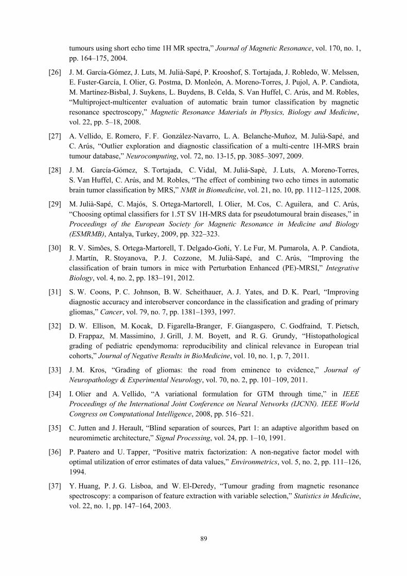
89

tumours using short echo time 1H MR spectra,” Journal of Magnetic Resonance, vol. 170, no. 1, pp. 164–175, 2004.

[26] J. M. García-Gómez, J. Luts, M. Julià-Sapé, P. Krooshof, S. Tortajada, J. Robledo, W. Melssen, E. Fuster-García, I. Olier, G. Postma, D. Monleón, A. Moreno-Torres, J. Pujol, A. P. Candiota, M. Martínez-Bisbal, J. Suykens, L. Buydens, B. Celda, S. Van Huffel, C. Arús, and M. Robles, “Multiproject-multicenter evaluation of automatic brain tumor classification by magnetic resonance spectroscopy,” Magnetic Resonance Materials in Physics, Biology and Medicine, vol. 22, pp. 5–18, 2008.

[27] A. Vellido, E. Romero, F. F. González-Navarro, L. A. Belanche-Muñoz, M. Julià-Sapé, and C. Arús, “Outlier exploration and diagnostic classification of a multi-centre 1H-MRS brain tumour database,” Neurocomputing, vol. 72, no. 13-15, pp. 3085–3097, 2009.

[28] J. M. García-Gómez, S. Tortajada, C. Vidal, M. Juliá-Sapè, J. Luts, A. Moreno-Torres, S. Van Huffel, C. Arús, and M. Robles, “The effect of combining two echo times in automatic brain tumor classification by MRS,” NMR in Biomedicine, vol. 21, no. 10, pp. 1112–1125, 2008.

[29] M. Julià-Sapé, C. Majós, S. Ortega-Martorell, I. Olier, M. Cos, C. Aguilera, and C. Arús, “Choosing optimal classifiers for 1.5T SV 1H-MRS data for pseudotumoural brain diseases,” in Proceedings of the European Society for Magnetic Resonance in Medicine and Biology (ESMRMB), Antalya, Turkey, 2009, pp. 322–323.

[30] R. V. Simões, S. Ortega-Martorell, T. Delgado-Goñi, Y. Le Fur, M. Pumarola, A. P. Candiota, J. Martín, R. Stoyanova, P. J. Cozzone, M. Julià-Sapé, and C. Arús, “Improving the classification of brain tumors in mice with Perturbation Enhanced (PE)-MRSI,” Integrative Biology, vol. 4, no. 2, pp. 183–191, 2012.

[31] S. W. Coons, P. C. Johnson, B. W. Scheithauer, A. J. Yates, and D. K. Pearl, “Improving diagnostic accuracy and interobserver concordance in the classification and grading of primary gliomas,” Cancer, vol. 79, no. 7, pp. 1381–1393, 1997.

[32] D. W. Ellison, M. Kocak, D. Figarella-Branger, F. Giangaspero, C. Godfraind, T. Pietsch, D. Frappaz, M. Massimino, J. Grill, J. M. Boyett, and R. G. Grundy, “Histopathological grading of pediatric ependymoma: reproducibility and clinical relevance in European trial cohorts,” Journal of Negative Results in BioMedicine, vol. 10, no. 1, p. 7, 2011.

[33] J. M. Kros, “Grading of gliomas: the road from eminence to evidence,” Journal of Neuropathology & Experimental Neurology, vol. 70, no. 2, pp. 101–109, 2011.

[34] I. Olier and A. Vellido, “A variational formulation for GTM through time,” in IEEE Proceedings of the International Joint Conference on Neural Networks (IJCNN). IEEE World Congress on Computational Intelligence, 2008, pp. 516–521.

[35] C. Jutten and J. Herault, “Blind separation of sources, Part 1: an adaptive algorithm based on neuromimetic architecture,” Signal Processing, vol. 24, pp. 1–10, 1991.

[36] P. Paatero and U. Tapper, “Positive matrix factorization: A non-negative factor model with optimal utilization of error estimates of data values,” Environmetrics, vol. 5, no. 2, pp. 111–126, 1994.

[37] Y. Huang, P. J. G. Lisboa, and W. El-Deredy, “Tumour grading from magnetic resonance spectroscopy: a comparison of feature extraction with variable selection,” Statistics in Medicine, vol. 22, no. 1, pp. 147–164, 2003.

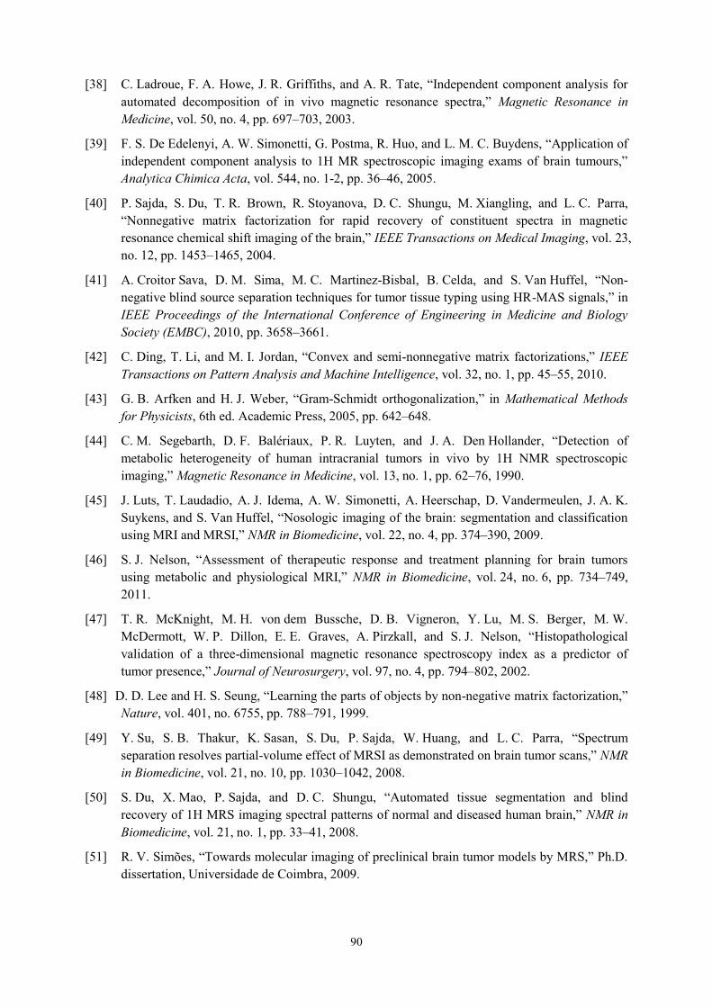
90

[38] C. Ladroue, F. A. Howe, J. R. Griffiths, and A. R. Tate, “Independent component analysis for automated decomposition of in vivo magnetic resonance spectra,” Magnetic Resonance in Medicine, vol. 50, no. 4, pp. 697–703, 2003.

[39] F. S. De Edelenyi, A. W. Simonetti, G. Postma, R. Huo, and L. M. C. Buydens, “Application of independent component analysis to 1H MR spectroscopic imaging exams of brain tumours,” Analytica Chimica Acta, vol. 544, no. 1-2, pp. 36–46, 2005.

[40] P. Sajda, S. Du, T. R. Brown, R. Stoyanova, D. C. Shungu, M. Xiangling, and L. C. Parra, “Nonnegative matrix factorization for rapid recovery of constituent spectra in magnetic resonance chemical shift imaging of the brain,” IEEE Transactions on Medical Imaging, vol. 23, no. 12, pp. 1453–1465, 2004.

[41] A. Croitor Sava, D. M. Sima, M. C. Martinez-Bisbal, B. Celda, and S. Van Huffel, “Non-negative blind source separation techniques for tumor tissue typing using HR-MAS signals,” in IEEE Proceedings of the International Conference of Engineering in Medicine and Biology Society (EMBC), 2010, pp. 3658–3661.

[42] C. Ding, T. Li, and M. I. Jordan, “Convex and semi-nonnegative matrix factorizations,” IEEE Transactions on Pattern Analysis and Machine Intelligence, vol. 32, no. 1, pp. 45–55, 2010.

[43] G. B. Arfken and H. J. Weber, “Gram-Schmidt orthogonalization,” in Mathematical Methods for Physicists, 6th ed. Academic Press, 2005, pp. 642–648.

[44] C. M. Segebarth, D. F. Balériaux, P. R. Luyten, and J. A. Den Hollander, “Detection of metabolic heterogeneity of human intracranial tumors in vivo by 1H NMR spectroscopic imaging,” Magnetic Resonance in Medicine, vol. 13, no. 1, pp. 62–76, 1990.

[45] J. Luts, T. Laudadio, A. J. Idema, A. W. Simonetti, A. Heerschap, D. Vandermeulen, J. A. K. Suykens, and S. Van Huffel, “Nosologic imaging of the brain: segmentation and classification using MRI and MRSI,” NMR in Biomedicine, vol. 22, no. 4, pp. 374–390, 2009.

[46] S. J. Nelson, “Assessment of therapeutic response and treatment planning for brain tumors using metabolic and physiological MRI,” NMR in Biomedicine, vol. 24, no. 6, pp. 734–749, 2011.

[47] T. R. McKnight, M. H. von dem Bussche, D. B. Vigneron, Y. Lu, M. S. Berger, M. W. McDermott, W. P. Dillon, E. E. Graves, A. Pirzkall, and S. J. Nelson, “Histopathological validation of a three-dimensional magnetic resonance spectroscopy index as a predictor of tumor presence,” Journal of Neurosurgery, vol. 97, no. 4, pp. 794–802, 2002.

[48] D. D. Lee and H. S. Seung, “Learning the parts of objects by non-negative matrix factorization,” Nature, vol. 401, no. 6755, pp. 788–791, 1999.

[49] Y. Su, S. B. Thakur, K. Sasan, S. Du, P. Sajda, W. Huang, and L. C. Parra, “Spectrum separation resolves partial-volume effect of MRSI as demonstrated on brain tumor scans,” NMR in Biomedicine, vol. 21, no. 10, pp. 1030–1042, 2008.

[50] S. Du, X. Mao, P. Sajda, and D. C. Shungu, “Automated tissue segmentation and blind recovery of 1H MRS imaging spectral patterns of normal and diseased human brain,” NMR in Biomedicine, vol. 21, no. 1, pp. 33–41, 2008.

[51] R. V. Simões, “Towards molecular imaging of preclinical brain tumor models by MRS,” Ph.D. dissertation, Universidade de Coimbra, 2009.

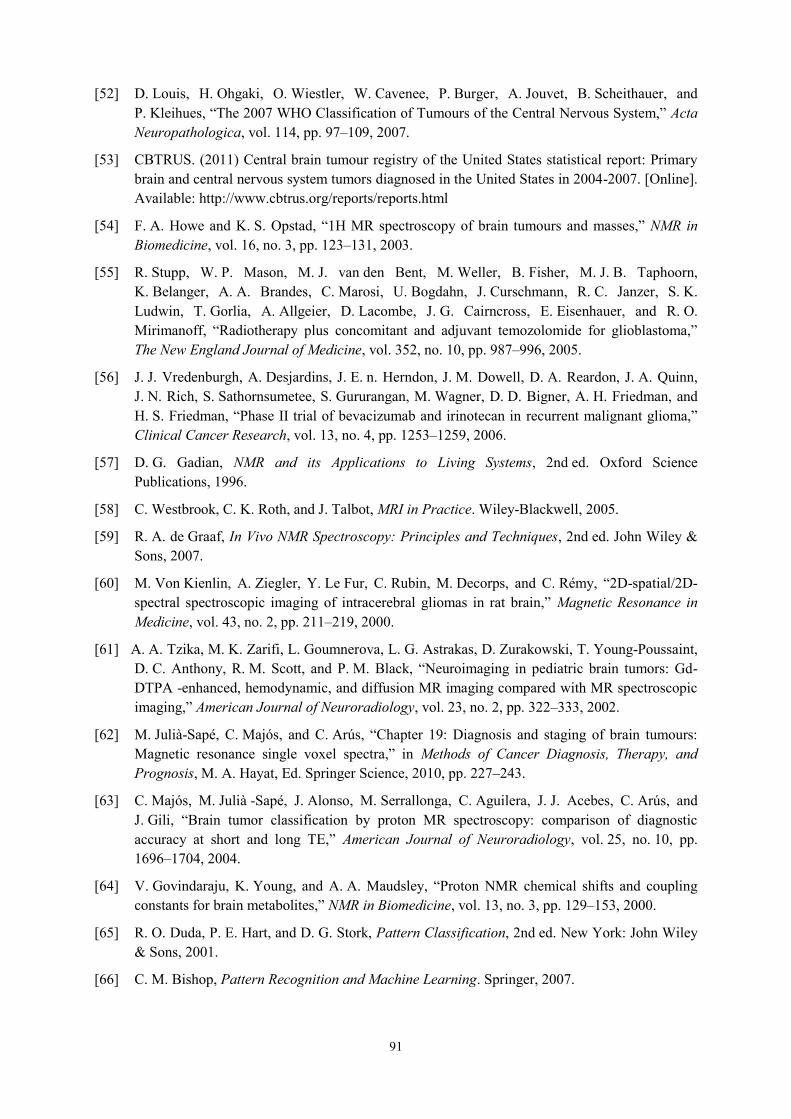
91

[52] D. Louis, H. Ohgaki, O. Wiestler, W. Cavenee, P. Burger, A. Jouvet, B. Scheithauer, and P. Kleihues, “The 2007 WHO Classification of Tumours of the Central Nervous System,” Acta Neuropathologica, vol. 114, pp. 97–109, 2007.

[53] CBTRUS. (2011) Central brain tumour registry of the United States statistical report: Primary brain and central nervous system tumors diagnosed in the United States in 2004-2007. [Online]. Available: http://www.cbtrus.org/reports/reports.html

[54] F. A. Howe and K. S. Opstad, “1H MR spectroscopy of brain tumours and masses,” NMR in Biomedicine, vol. 16, no. 3, pp. 123–131, 2003.

[55] R. Stupp, W. P. Mason, M. J. van den Bent, M. Weller, B. Fisher, M. J. B. Taphoorn, K. Belanger, A. A. Brandes, C. Marosi, U. Bogdahn, J. Curschmann, R. C. Janzer, S. K. Ludwin, T. Gorlia, A. Allgeier, D. Lacombe, J. G. Cairncross, E. Eisenhauer, and R. O. Mirimanoff, “Radiotherapy plus concomitant and adjuvant temozolomide for glioblastoma,” The New England Journal of Medicine, vol. 352, no. 10, pp. 987–996, 2005.

[56] J. J. Vredenburgh, A. Desjardins, J. E. n. Herndon, J. M. Dowell, D. A. Reardon, J. A. Quinn, J. N. Rich, S. Sathornsumetee, S. Gururangan, M. Wagner, D. D. Bigner, A. H. Friedman, and H. S. Friedman, “Phase II trial of bevacizumab and irinotecan in recurrent malignant glioma,” Clinical Cancer Research, vol. 13, no. 4, pp. 1253–1259, 2006.

[57] D. G. Gadian, NMR and its Applications to Living Systems, 2nd ed. Oxford Science Publications, 1996.

[58] C. Westbrook, C. K. Roth, and J. Talbot, MRI in Practice. Wiley-Blackwell, 2005.

[59] R. A. de Graaf, In Vivo NMR Spectroscopy: Principles and Techniques, 2nd ed. John Wiley & Sons, 2007.

[60] M. Von Kienlin, A. Ziegler, Y. Le Fur, C. Rubin, M. Decorps, and C. Rémy, “2D-spatial/2D-spectral spectroscopic imaging of intracerebral gliomas in rat brain,” Magnetic Resonance in Medicine, vol. 43, no. 2, pp. 211–219, 2000.

[61] A. A. Tzika, M. K. Zarifi, L. Goumnerova, L. G. Astrakas, D. Zurakowski, T. Young-Poussaint, D. C. Anthony, R. M. Scott, and P. M. Black, “Neuroimaging in pediatric brain tumors: Gd-DTPA -enhanced, hemodynamic, and diffusion MR imaging compared with MR spectroscopic imaging,” American Journal of Neuroradiology, vol. 23, no. 2, pp. 322–333, 2002.

[62] M. Julià-Sapé, C. Majós, and C. Arús, “Chapter 19: Diagnosis and staging of brain tumours: Magnetic resonance single voxel spectra,” in Methods of Cancer Diagnosis, Therapy, and Prognosis, M. A. Hayat, Ed. Springer Science, 2010, pp. 227–243.

[63] C. Majós, M. Julià -Sapé, J. Alonso, M. Serrallonga, C. Aguilera, J. J. Acebes, C. Arús, and J. Gili, “Brain tumor classification by proton MR spectroscopy: comparison of diagnostic accuracy at short and long TE,” American Journal of Neuroradiology, vol. 25, no. 10, pp. 1696–1704, 2004.

[64] V. Govindaraju, K. Young, and A. A. Maudsley, “Proton NMR chemical shifts and coupling constants for brain metabolites,” NMR in Biomedicine, vol. 13, no. 3, pp. 129–153, 2000.

[65] R. O. Duda, P. E. Hart, and D. G. Stork, Pattern Classification, 2nd ed. New York: John Wiley & Sons, 2001.

[66] C. M. Bishop, Pattern Recognition and Machine Learning. Springer, 2007.

92

[67] A. Vellido, E. Romero, M. Julià-Sapé, C. Majós, A. Moreno-Torres, J. Pujol, and C. Arús, “Robust discrimination of glioblastomas from metastatic brain tumors on the basis of single-voxel 1H MRS,” NMR in Biomedicine, vol. In press. DOI:10.1002/nbm.1797, 2011.

[68] J. A. Osorio, E. Ozturk-Isik, D. Xu, S. Cha, S. Chang, M. S. Berger, D. B. Vigneron, and S. J. Nelson, “3D 1H MRSI of brain tumors at 3.0 tesla using an eight-channel phased-array head coil,” Journal of Magnetic Resonance Imaging, vol. 26, no. 1, pp. 23–30, 2007.

[69] T. W. J. Scheenen, D. W. J. Klomp, J. P. Wijnen, and A. Heerschap, “Short echo time 1H-MRSI of the human brain at 3T with minimal chemical shift displacement errors using adiabatic refocusing pulses,” Magnetic Resonance in Medicine, vol. 59, no. 1, pp. 1–6, 2008.

[70] T. Scheenen, A. Heerschap, and D. Klomp, “Towards 1H-MRSI of the human brain at 7T with slice-selective adiabatic refocusing pulses,” Magnetic Resonance Materials in Physics, Biology and Medicine, vol. 21, pp. 95–101, 2008.

[71] V. Mlynárik, I. Kohler, G. Gambarota, A. Vaslin, P. G. Clarke, and R. Gruetter, “Quantitative proton spectroscopic imaging of the neurochemical profile in rat brain with microliter resolution at ultra-short echo times,” Magnetic Resonance in Medicine, vol. 59, no. 1, pp. 52–58, 2008.

[72] M. von Kienlin, A. Ziegler, Y. Le Fur, C. Rubin, M. Décorps, and C. Rémy, “2D-spatial/2D-spectral spectroscopic imaging of intracerebral gliomas in rat brain,” Magnetic Resonance in Medicine, vol. 43, no. 2, pp. 211–219, 2000.

[73] M. L. García-Martín, G. Hérigault, C. Rémy, R. Farion, P. Ballesteros, J. A. Coles, S. Cerdán, and A. Ziegler, “Mapping extracellular pH in rat brain gliomas in vivo by H magnetic resonance spectroscopic imaging: Comparison with maps of metabolites,” Cancer Research, vol. 61, no. 17, pp. 6524–6531, 2001.

[74] T. J. Liimatainen, A. T. Erkkilä, P. Valonen, H. Vidgren, M. Lakso, G. Wong, O. H. Gröhn, S. Ylä-Herttuala, and J. M. Hakumäki, “1H MR spectroscopic imaging of phospholipase-mediated membrane lipid release in apoptotic rat glioma in vivo,” Magnetic Resonance in Medicine, vol. 59, no. 6, pp. 1232–1238, 2008.

[75] M. D. Boska, T. B. Lewis, C. J. Destache, E. J. Benner, J. A. Nelson, M. Uberti, R. L. Mosley, and H. E. Gendelman, “Quantitative 1H magnetic resonance spectroscopic imaging determines therapeutic immunization efficacy in an animal model of Parkinson’s disease,” The Journal of Neuroscience, vol. 25, no. 7, pp. 1691–1700, 2005.

[76] J. A. Nelson, H. Dou, B. Ellison, M. Uberti, H. Xiong, E. Anderson, M. Mellon, H. A. Gelbard, M. Boska, and H. E. Gendelman, “Coregistration of quantitative proton magnetic resonance spectroscopic imaging with neuropathological and neurophysiological analyses defines the extent of neuronal impairments in murine human immunodeficiency virus type-1 encephalitis,” Journal of Neuroscience Research, vol. 80, no. 4, pp. 562–575, 2005.

[77] P. J. G. Lisboa, E. Romero, A. Vellido, M. Julià-Sapé, and C. Arus, “Classification, dimensionality reduction, and maximally discriminatory visualization of a multicentre 1H-MRS database of brain tumors,” in IEEE Proceedings of the International Conference on Machine Learning and Applications (ICMLA), 2008, pp. 613 –618.

[78] I. Guyon and A. Elisseeff, “An introduction to variable and feature selection,” Journal of Machine Learning Research, vol. 3, pp. 1157–1182, 2003.

[79] T. Hastie, R. Tibshirani, and J. Friedman, The Elements of Statistical Learning: Data Mining, Inference, and Prediction (Second Edition), ser. Springer Series in Statistics. Springer, 2008.

93

[80] M. A. Hall, “Correlation-based feature selection for discrete and numeric class machine learning,” in Proceedings of the 17th International Conference on Machine Learning. Morgan Kaufmann, San Francisco, CA, 2000, pp. 359–366.

[81] A. K. Jain, R. P. W. Duin, and M. Jianchang, “Statistical pattern recognition: a review,” IEEE Transactions on Pattern Analysis and Machine Intelligence, vol. 22, no. 1, pp. 4–37, 2000.

[82] B. Efron and R. J. Tibshirani, An introduction to the Bootstrap, ser. Monographs on Statistics and Applied Probability, 57. Chapman & Hall, 1998.

[83] T. Fawcett, “An introduction to ROC analysis,” Pattern Recognition Letters, vol. 27, no. 8, pp. 861–874, 2006.

[84] D. G. Altman and P. Royston, “What do we mean by validating a prognostic model?” Statistics in Medicine, vol. 19, no. 4, pp. 453–473, 2000.

[85] A. Hyvärinen and E. Oja, “Independent component analysis: algorithms and applications,” Neural Networks, vol. 13, pp. 411–430, 2000.

[86] J. F. Cardoso and A. Souloumiac, “Blind beamforming for non-Gaussian signals,” IEE Proceedings F Radar and Signal Processing, vol. 140, no. 6, pp. 362–370, 1993.

[87] A. Hyvärinen, “Fast and robust fixed-point algorithms for independent component analysis,” IEEE Transactions on Neural Networks, vol. 10, no. 3, pp. 626–634, 1999.

[88] C. J. Lin, “Projected gradient methods for nonnegative matrix factorization,” Neural Computation, vol. 19, pp. 2756–2779, 2007.

[89] B. Hassibi and D. G. Stork, “Second order derivatives for network pruning: Optimal brain surgeon,” Advances in Neural Information Processing Systems, vol. 5, pp. 164–171, 1993.

[90] IMM, Technical University of Denmark. (2006) NMF: DTU Toolbox. Collection of NMF algorithms implemented for Matlab. [Online]. Available: http://cogsys.imm.dtu.dk/toolbox/nmf.

[91] X. Ding, J.-H. Lee, and S.-W. Lee, “A constrained alternating least squares nonnegative matrix factorization algorithm enhances task-related neuronal activity detection from single subject’s fMRI data,” in Proceedings of the International Conference on Machine Learning and Cybernetics (ICMLC), vol. 1, 2011, pp. 338–343.

[92] SPSS Inc. SPSS. [Online]. Available: http://www.spss.com/

[93] SAS Institute Inc. SAS. [Online]. Available: http://www.sas.com/

[94] Umetrics. SIMCA-P+. [Online]. Available: http://www.umetrics.com/simca

[95] R. Ihaka and R. Gentleman, “R: a language for data analysis and graphics,” Journal of Computational and Graphical Statistics, vol. 5, no. 3, pp. 299–314, 1996.

[96] The MathWorks, Inc. (1994-2012) MATLAB. [Online]. Available: http://-www.mathworks.com/

[97] Bruker BioSpin. AMIX: exploring of spectroscopic data. [Online]. Available: http://-www.bruker-biospin.com/amix.html

[98] Infometrix. Pirouette. [Online]. Available: http://www.infometrix.com/software/pirouette.html

[99] S. Ortega-Martorell, I. Olier, M. Julià-Sapé, and C. Arús, “SpectraClassifier 1.0: a user friendly, automated MRS-based classifier-development system,” BMC Bioinformatics, vol. 11, p. 106, 2010.

94

[100] I. Olier and A. Vellido, “Advances in clustering and visualization of time series using GTM through time,” Neural Networks, vol. 21, no. 7, pp. 904–913, 2008.

[101] C. Bishop, M. Svensén, and C. Williams, “GTM: The generative topographic mapping,” Neural Computation, vol. 10, pp. 215–234, 1998.

[102] T. Kohonen, Self-Organizing Maps, 3rd ed. New York: Springer, 2001, vol. 30.

[103] I. Olier, “Variational Bayesian Algorithms for Generative Topographic Mapping and its Extensions,” Ph.D. dissertation, Universitat Politécnica de Catalunya, 2008.

[104] A. Vellido, “Missing data imputation through GTM as a mixture of t-distributions,” Neural Networks, vol. 19, no. 10, pp. 1624–1635, 2006.

[105] I. Olier and A. Vellido, “Comparative assessment of the robustness of missing data imputation through Generative Topographic Mapping,” in Proceedings of Computational Intelligence and Bioinspired Systems, ser. Lecture Notes in Computer Science, vol. 3512/2005. Springer Berlin, 2005, pp. 787–794.

[106] A. Vellido and P. J. G. Lisboa, “Handling outliers in brain tumour MRS data analysis through robust topographic mapping,” Computers in Biology and Medicine, vol. 36, no. 10, pp. 1049–1063, 2006.

[107] A. Vellido, “Preliminary theoretical results on a feature relevance determination method for Generative Topographic Mapping,” Universitat Politécnica de Catalunya, Tech. Rep., 2005.

[108] C. M. Bishop, G. E. Hinton, and I. G. D. Strachan, “GTM through time,” in Proceedings of the International Conference on Artificial Neural Networks, 1997, pp. 111–116.

[109] I. Olier and A. Vellido, “Capturing the dynamics of multivariate time series through visualization using Generative Topographic Mapping Through Time,” in IEEE Proceedings of the International Conference on Engineering of Intelligent Systems, 2006, pp. 1–6.

[110] S. Ortega-Martorell, A. Vellido, P. J. Lisboa, M. Julià-Sapé, and C. Arús, “Spectral decomposition methods for the analysis of MRS information from human brain tumors,” in IEEE Proceedings of the International Joint Conference on Neural Networks (IJCNN), San José, California, USA, 2011, pp. 3279–3284.

[111] Z. Zhenga, J. Yangb, and Y. Zhuc, “Initialization enhancer for non-negative matrix factorization,” Engineering Applications of Artificial Intelligence, vol. 20, no. 1, pp. 101–110, 2007.

[112] A. Langville, C. Meyer, and R. Albright, “Initializations for the nonnegative matrix factorization,” in Proceedings of the 12th ACM SIGKDD International Conference on Knowledge Discovery and Data Mining, Philadelphia, PA, USA, 2006.

[113] J. Luts, J.-B. Poullet, J. M. Garcia-Gomez, A. Heerschap, M. Robles, J. A. K. Suykens, and S. V. Huffel, “Effect of feature extraction for brain tumor classification based on short echo time 1H MR spectra,” Magnetic Resonance in Medicine, vol. 60, no. 2, pp. 288–298, 2008.

[114] F. Colas, J. N. Kok, and A. Vellido, “Finding discriminative subtypes of aggressive brain tumours using magnetic resonance spectroscopy,” in IEEE Proceedings of the International Conference of Engineering in Medicine and Biology Society (EMBC), 2010, pp. 1065 –1068.

[115] C. Majós, J. Bruna, M. Julià-Sapé, M. Cos, A. Camins, M. Gil, J. J. Acebes, C. Aguilera, and C. Arús, “Proton MR spectroscopy provides relevant prognostic information in high-grade astrocytomas,” American Journal of Neuroradiology, vol. 32, pp. 74–80, 2011.

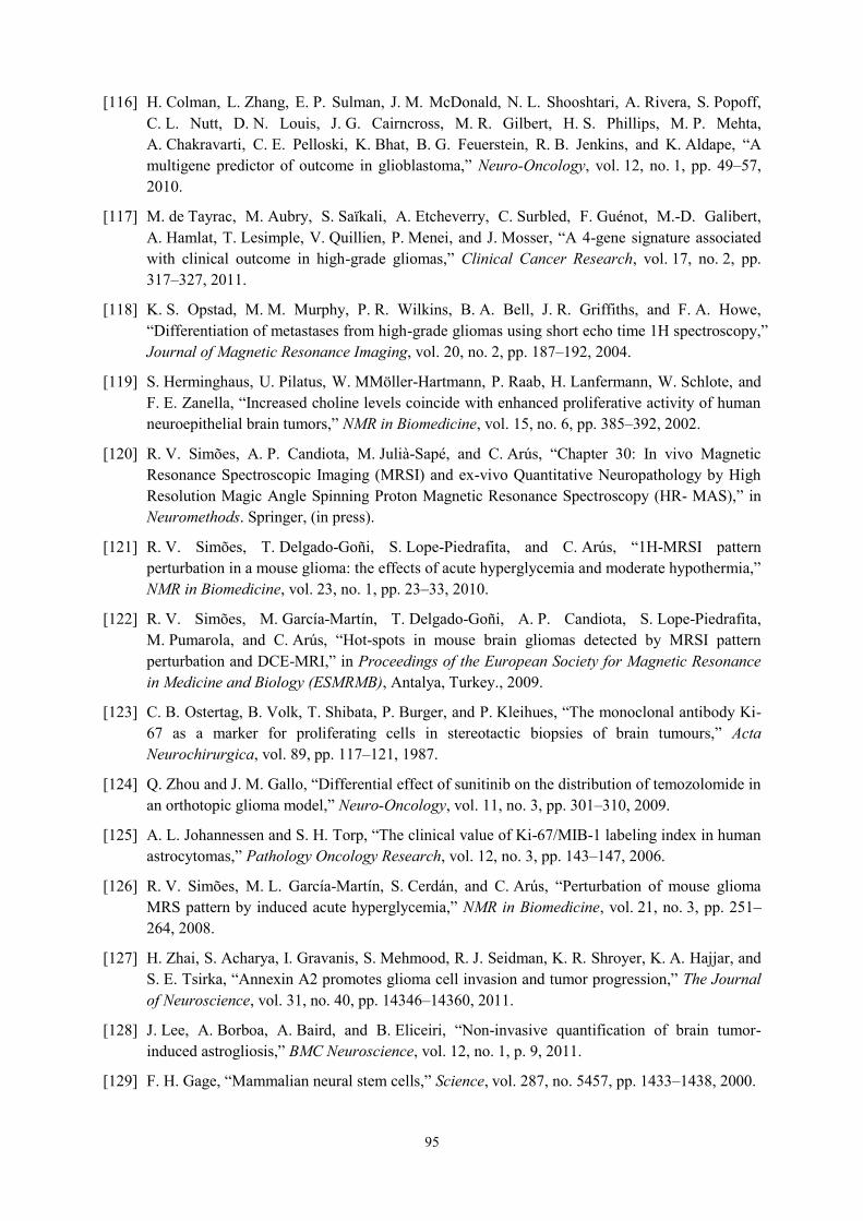
95

[116] H. Colman, L. Zhang, E. P. Sulman, J. M. McDonald, N. L. Shooshtari, A. Rivera, S. Popoff, C. L. Nutt, D. N. Louis, J. G. Cairncross, M. R. Gilbert, H. S. Phillips, M. P. Mehta, A. Chakravarti, C. E. Pelloski, K. Bhat, B. G. Feuerstein, R. B. Jenkins, and K. Aldape, “A multigene predictor of outcome in glioblastoma,” Neuro-Oncology, vol. 12, no. 1, pp. 49–57, 2010.

[117] M. de Tayrac, M. Aubry, S. Saïkali, A. Etcheverry, C. Surbled, F. Guénot, M.-D. Galibert, A. Hamlat, T. Lesimple, V. Quillien, P. Menei, and J. Mosser, “A 4-gene signature associated with clinical outcome in high-grade gliomas,” Clinical Cancer Research, vol. 17, no. 2, pp. 317–327, 2011.

[118] K. S. Opstad, M. M. Murphy, P. R. Wilkins, B. A. Bell, J. R. Griffiths, and F. A. Howe, “Differentiation of metastases from high-grade gliomas using short echo time 1H spectroscopy,” Journal of Magnetic Resonance Imaging, vol. 20, no. 2, pp. 187–192, 2004.

[119] S. Herminghaus, U. Pilatus, W. MMöller-Hartmann, P. Raab, H. Lanfermann, W. Schlote, and F. E. Zanella, “Increased choline levels coincide with enhanced proliferative activity of human neuroepithelial brain tumors,” NMR in Biomedicine, vol. 15, no. 6, pp. 385–392, 2002.

[120] R. V. Simões, A. P. Candiota, M. Julià-Sapé, and C. Arús, “Chapter 30: In vivo Magnetic Resonance Spectroscopic Imaging (MRSI) and ex-vivo Quantitative Neuropathology by High Resolution Magic Angle Spinning Proton Magnetic Resonance Spectroscopy (HR- MAS),” in Neuromethods. Springer, (in press).

[121] R. V. Simões, T. Delgado-Goñi, S. Lope-Piedrafita, and C. Arús, “1H-MRSI pattern perturbation in a mouse glioma: the effects of acute hyperglycemia and moderate hypothermia,” NMR in Biomedicine, vol. 23, no. 1, pp. 23–33, 2010.

[122] R. V. Simões, M. García-Martín, T. Delgado-Goñi, A. P. Candiota, S. Lope-Piedrafita, M. Pumarola, and C. Arús, “Hot-spots in mouse brain gliomas detected by MRSI pattern perturbation and DCE-MRI,” in Proceedings of the European Society for Magnetic Resonance in Medicine and Biology (ESMRMB), Antalya, Turkey., 2009.

[123] C. B. Ostertag, B. Volk, T. Shibata, P. Burger, and P. Kleihues, “The monoclonal antibody Ki-67 as a marker for proliferating cells in stereotactic biopsies of brain tumours,” Acta Neurochirurgica, vol. 89, pp. 117–121, 1987.

[124] Q. Zhou and J. M. Gallo, “Differential effect of sunitinib on the distribution of temozolomide in an orthotopic glioma model,” Neuro-Oncology, vol. 11, no. 3, pp. 301–310, 2009.

[125] A. L. Johannessen and S. H. Torp, “The clinical value of Ki-67/MIB-1 labeling index in human astrocytomas,” Pathology Oncology Research, vol. 12, no. 3, pp. 143–147, 2006.

[126] R. V. Simões, M. L. García-Martín, S. Cerdán, and C. Arús, “Perturbation of mouse glioma MRS pattern by induced acute hyperglycemia,” NMR in Biomedicine, vol. 21, no. 3, pp. 251–264, 2008.

[127] H. Zhai, S. Acharya, I. Gravanis, S. Mehmood, R. J. Seidman, K. R. Shroyer, K. A. Hajjar, and S. E. Tsirka, “Annexin A2 promotes glioma cell invasion and tumor progression,” The Journal of Neuroscience, vol. 31, no. 40, pp. 14346–14360, 2011.

[128] J. Lee, A. Borboa, A. Baird, and B. Eliceiri, “Non-invasive quantification of brain tumor-induced astrogliosis,” BMC Neuroscience, vol. 12, no. 1, p. 9, 2011.

[129] F. H. Gage, “Mammalian neural stem cells,” Science, vol. 287, no. 5457, pp. 1433–1438, 2000.

96

[130] R. Glass, M. Synowitz, G. Kronenberg, J. H. Walzlein, D. S. Markovic, L. P. Wang, D. Gast, J. Kiwit, G. Kempermann, and H. Kettenmann, “Glioblastoma-induced attraction of endogenous neural precursor cells is associated with improved survival,” The Journal of Neuroscience, vol. 25, no. 10, pp. 2637–2646, 2005.

[131] R. Bitar, G. Leung, R. Perng, S. Tadros, A. R. Moody, J. Sarrazin, C. McGregor, M. Christakis, S. Symons, A. Nelson, and T. P. Roberts, “MR pulse sequences: what every radiologist wants to know but is afraid to ask,” Radiographics, vol. 26, no. 2, pp. 513–537, 2006.

[132] I. Park, R. Bok, T. Ozawa, J. J. Phillips, C. D. James, D. B. Vigneron, S. M. Ronen, and S. J. Nelson, “Detection of early response to temozolomide treatment in brain tumors using hyperpolarized 13C MR metabolic imaging,” Journal of Magnetic Resonance Imaging, vol. 33, no. 6, pp. 1284–1290, 2011.

[133] M. M. Chaumeil, T. Ozawa, I. Park, K. Scott, C. D. James, S. J. Nelson, and S. M. Ronen, “Hyperpolarized 13C MR spectroscopic imaging can be used to monitor Everolimus treatment in vivo in an orthotopic rodent model of glioblastoma,” NeuroImage, vol. 59, no. 1, pp. 193–201, 2012.

[134] M. De Vos, T. Laudadio, A. Simonetti, A. Heerschap, and S. Van Huffel, “Fast nosologic imaging of the brain,” Journal of Magnetic Resonance, vol. 184, no. 2, pp. 292–301, 2007.

[135] A. Pirzkall, X. Li, J. Oh, S. Chang, M. S. Berger, D. A. Larson, L. J. Verhey, W. P. Dillon, and S. J. Nelson, “3D MRSI for resected high-grade gliomas before RT: tumor extent according to metabolic activity in relation to MRI,” International Journal of Radiation Oncology, Biology, Physics, vol. 59, no. 1, pp. 126–137, 2004.

[136] H. Ruiz, S. Ortega-Martorell, I. H. Jarman, A. Vellido, E. Romero, J. D. Martín, and P. J. G. Lisboa, “Towards interpretable classifiers with blind signal separation,” in IEEE Proceedings of the International Joint Conference on Neural Networks (IJCNN), Brisbane, Australia, 2012.

on the use of advanced pattern recognition techniques for ... · para la aplicación de técnicas...

Documents