on the weber facility location problem with limited

Noname manuscript No.(will be inserted by the editor)

On the Weber facility location problem with limited

distances and side constraints

Isaac F. Fernandes · Daniel Aloise ·

Dario J. Aloise · Pierre Hansen · Leo

Liberti

Received: date / Accepted: date

Abstract The objective in the continuous facility location problem with lim-ited distances is to minimize the sum of distance functions from the facilityto the customers, but with a limit on each of the distances, after which thecorresponding function becomes constant. The problem has applications insituations where the service provided by the facility is insensitive after a giventhreshold distance. In this paper, we propose a global optimization algorithmfor the case in which there are in addition lower and upper bounds on thenumbers of customers served.

Keywords facility location · global optimization · reformulation · decompo-sition

1 Introduction

The continuous minisum single facility problem is one of the most fundamentalproblems in location theory. The objective is to locate a single facility in theplane so that the sum of distances from the facility to a set of demand pointsis minimized. The problem is often referred to in the literature as the Weber(or Fermat-Weber) problem [4,16,18]. It traces back to Fermat in the 17th

I. Fernandes, D. Aloise and D.J. AloiseUniversidade Federal do Rio Grande do Norte, Campus Universitario s/n, Natal-RN, Brazil,59072-970E-mail: [email protected], [email protected], [email protected]

P. HansenGERAD and HEC Montreal, 3000, Chemin de la Cote-Sainte-Catherine, Montreal, Quebec,Canada, H3T 2A7E-mail: [email protected]

L. LibertiLIX, Ecole Polytechnique, F-91128, Palaiseau, FranceE-mail: [email protected]

2 Isaac F. Fernandes et al.

century who posed a purely geometrical version of the problem with only threepoints. Torricelli, in 1647, is credited to prove that the circles circumscribingthe equilateral triangles constructed on the sides of the triangle formed bythe three given points intersect in the fourth point sought (see [24,26] for ahistorical survey).

Drezner, Mehrez and Wesolowsky investigated in [13] the Weber problemfor the case in which the distance functions are constant after given thresh-old values, which they call the facility location problem with limited distances.This problem has applications in situations where the service provided by thefacility is insensitive after a given threshold time/distance. For instance, con-sider the problem of locating a fire station. In this context, each property hasa distance limit after which the service provided by the firemen is useless,and the property is completely destroyed. An example of this operations re-search application is provided in [13]. The authors suppose a situation wherea certain damage occurs in a property located in pi for i = 1, . . . , n at zerodistance from the fire station (located at y ∈ R

2), and that this damage lin-early increases up to a distance λi where the damage is 100%. By denotingd(pi, y) the distance between point pi and the facility located at y, and Ωthe proportion of damage at zero distance, the proportion of damage in pi isgiven by Ω+(1−Ω)d(pi, y)/λi in the case d(pi, y) < λi, and 1 otherwise. Thecorresponding facility location problem is then expressed as

miny∈R2

n∑

i=1

Ω + (1−Ω)mind(pi, y), λi

λi(1)

The first term of the summation is constant and (1−Ω) is irrelevant to the sec-ond term. By introducing binary variables vi, that select between d(pi, y) andλi, to the summation of the objective function, we end up with the followingminimization problem

miny∈R2,v∈0,1n

n∑

i=1

1

λi(λi(1− vi) + d(pi, y)vi) . (2)

Real examples for the application of this location model also include othertypes of emergency services (e.g. ambulances, police calls). For example, aperson suffering from a heart attack has more chances to survive if he/she isquickly treated, and will certainly die if help does not come after a given periodof time. In the case of a police call, criminals would be likely untraceable aftera time limit.

In this work, we study the version of the problem for which there are lowerand upper bounds on the number of demand points that can be served withinthe distance limits. This is indeed a natural extension to the model presentedin [13]. In practical applications, a lower bound in the number of served pointsmay be used to justify the installation of a facility (e.g. it is not reasonable toconstruct a fire station that can save only a few properties nearby), while anupper bound may express the capacity limitations of the service to maintainan acceptable quality level.

Title Suppressed Due to Excessive Length 3

Another extension to the facility location problem with limited distancesformulated in [13] is presented by Drezner, Wesolowsky and Drezner in [15].In this paper, the authors formulate a problem in which the distance functionfrom the demand point is equal to zero up to a first threshold value l, linearbetween l and a second threshold distance value u, and constant after u. Themodel is equivalent to that of [13] when l = 0. In one hand, the mathemat-ical developments presented here cannot be used to help solving the globaloptimization problem presented in [15], at least not straightforwardly. On theother hand, adding the side constraints to the model of [15] would require aconsiderable effort on investigating new lower and upper bounds to be used ina specialized branch-and-bound. We decided to work on an extension to themodel of [13] by means of convex exact reformulations in the sense of [20].This yielded an enumerative algorithm based only on the resolution of convexproblems.

An adjacent facility location problem to the one approached here is theMaximal Covering Location Problem (MCLP) [8,9,21] which maximizes thenumber of demand points covered within a specified critical distance or timeby a fixed number of facilities. Although these models also incorporate facilitydistance limitations, they deal with a covering objective function which ismathematically distinct from the minisum objective. Covering problems are achapter apart in the facility location theory (see [3,22,14] for a survey).

The mathematical formulation of the problem approached in this paper isgiven in the next section. A global optimization algorithm for it is describedin Section 3. Computational results on synthesized instances and on a real-lifeproblem are reported in Section 4 and compared with those of the literature.Finally, conclusion are given in the last section.

2 Problem definition

Let us denote ‖p1−p2‖q the ℓq-distance between points p1 and p2 in the plane.Given n service points in the plane p1, p2, . . . , pn with threshold distancesλi > 0 and weights wi ≥ 0 for i = 1, . . . , n, the Limited Distance MinisumProblem with Side Constraints (LDMPSC) can be expressed by:

miny∈R2,v∈0,1n

n∑

i=1

wi (λi(1− vi) + ‖pi − y‖qvi)

subject to

‖pi − y‖qvi ≤ λi for i = 1, . . . , n (3)

L ≤n∑

i=1

vi ≤ U.

The first set of constraints defines bounds L and U in the number of variablesvi which can be equal to 1. The second set of constraints assures that vi canbe equal to 1 only if the distance between pi and the facility located at y is


inferior (or equal) to the distance limit λi. This avoids the attribution vi = 1only to satisfy constraint

∑ni=1

vi ≥ L. The objective function of (3) as wellas its feasible set are non convex which demands more sophisticated solutionmethods.

The objective function of (3) can still be rewritten thereby removing itsconstant terms. It is then expressed as

n∑

i=1

wiλi +min

n∑

i=1

wi(‖pi − y‖q − λi)vi. (4)

3 Optimization algorithm

From the formulation above, we have that for a given location y, vi may beequal to 1 only if ‖pi − y‖q ≤ λi. If q = 2, this is geometrically equivalentin the plane to the condition that vi may be equal to 1 only if y belongs toa disc Di = y|‖pi − y‖2 ≤ λi (i.e., a disc with radius λi centered at pi).Analogously, if q = 1, this is equivalent to the condition that vi may be equalto 1 only if y belongs to a square Si = y|‖pi − y‖1 ≤ λi with sides making a45 (or -45) degree angle with the axes (i.e., a 45 degrees rotated square withdiagonal 2λi centered at pi).

A branch-and-bound algorithm based on the vector v would consider im-plicitly all 2n subproblems generated by branching on binary variables vi fori = 1, . . . , n, while adding constraints ‖pi− y‖q ≤ λi and ‖pi− y‖q ≥ λi to theresulting subproblems. Another possibility is to focus on components vi of vwhich might be equal to 1 at the same time. When q = 2, these componentsare directly associated to convex regions generated by intersections of discs(see Figure 1). For instance, for the region indicated by the bullet in Figure 1,only the components v1, v2 and v3 can be equal to 1.

Hence, we can solve (3) by solving subproblems of the following type:

miny∈R2,v∈0,1|S|

∑

i∈S

wi(‖pi − y‖q − λi)vi

subject to

‖pi − y‖q ≤ λi ∀i ∈ S, (5)

L ≤∑

i∈S

vi ≤ U

where S ⊆ 1, 2, . . . , n is a non-empty set. Each one of the subproblemsof type (5) is associated to a distinct region in the plane. For instance, wehave a subproblem with S = 1, 2, 3 for the region indicated by the bulletin Figure 1. The number of these convex regions for q ≥ 1 was proved to bequadratically bounded in the number of points in [13].1

1 the proof omits a case. We completed the proof for q = 2 in [1].


p6

λ2

λ6

λ3

λ4

λ5

p3

p5

p4

p2

λ1p1

Fig. 1 Intersection of discs.

Problem (5) contains (nonconvex) bilinear terms in the objective function,so that its continuous relaxation is not necessarily easy to solve. To addressthis issue we propose the following reformulation of (5): we add variableszi ∈ [−λi, 0] for all i ∈ S, we replace the objective function with

∑

i∈S wizi,and adjoin the following constraints:

∀i ∈ S ‖pi − y‖q − λi ≤ zi (6)

∀i ∈ S zi + λivi ≥ 0. (7)

We remark that the original constraints ∀i ∈ S (‖pi − y‖q ≤ λi) are also partof the reformulation, as well as bound and integrality constraints on y, v. Theresulting reformulation:


∑

i∈S

wizi

∀i ∈ S ‖pi − y‖q − λi ≤ zi∀i ∈ S zi + λivi ≥ 0∀i ∈ S ‖pi − y‖q ≤ λi

L ≤∑

i∈S vi ≤ U∀i ∈ S zi ∈ [−λi, 0].

(8)

is an exact reformulation of (5), i.e. the optima of (8) can be mapped surjec-tively onto the optima of (5) [20], as shown in Prop. 1. We also remark that(8) is a convex Mixed-Integer Nonlinear Program (MINLP), as it involves con-tinuous and integer variables as well as nonlinear terms, and its continuousrelaxation is a convex Nonlinear Program (NLP). This is because: (i) all normsare convex functions [7, p. 73], (ii) adding a linear function to a convex one


results in a convex function, and (iii) bounding convex functions from abovedefines a convex set.

Proposition 1 Prob. (8) is an exact reformulation of Prob. (5).

Proof Let (y∗, v∗, z∗) be an optimal solution of (8). For i ∈ S, if v∗i = 0 then,because ‖pi−y∗‖q ≤ λi, the left hand side of (6) is nonpositive; hence, by (7),z∗i ≥ 0 is the most stringent constraint. By the upper bound constraint on z, wehave z∗i = 0. If v∗i = 1, (7) implies z∗i ≥ −λi, which is redundant with respect tothe lower bound constraint on z. Hence, by (6), we have z∗i ≥ ‖pi − y∗‖q − λi,and the objective function direction enforces z∗i = ‖pi − y∗‖q − λi. Thus,the optimal objective function value of (8) is the same as that of (5) at theoptimum (y∗, v∗) of (5). As concerns surjectivity, it is easy to remark that foreach feasible (y, v) in (5) there exist a corresponding z such that (y, v, z) isfeasible in (8): simply define zi = (‖pi − y‖q − λi)vi. Hence, the projectionoperator of the optima of (8) onto the variables of (5) is surjective on theoptima on (5) and certifies that the reformulation is exact.

For q = 1, Prob. (8) is a Mixed Integer Linear Program (MILP); this follows bya classical exact reformulation of convex constraints involving absolute values|x| ≤ r into pairs of constraints −r ≤ x ≤ r. For example, ‖pi − y‖1 =|pi1 − y1|+ |pi2 − y2| ≤ λi is initially replaced by:

pi1 − y1 ≤ λi − |pi2 − y2| and pi1 − y1 ≥ |pi2 − y2| − λi.

Then, each of the constraints above is replaced by two others, yielding theconstraints:

y1 + y2 ≥ pi1 + pi2 − λi

y1 − y2 ≥ pi1 − pi2 − λi

y1 − y2 ≤ pi1 − pi2 + λi

y1 + y2 ≤ pi1 + pi2 + λi.

For q = 2, Prob. (8) is a convex MINLP. Due to the presence of the squareroot term in the Euclidean norm, the problem is not everywhere differentiable.Specifically, this sometimes causes floating-point errors in local NLP solvers,but there exist practically efficient convex MINLP solvers for this type ofproblems (e.g. Bonmin [5]).

Proposition 2 shows that the resolution of subproblems can still be furthersimplified, allowing to solve simpler subproblems whenever their size (i.e., |S|)is not greater than U .

Proposition 2 There exists a solution (y∗, v∗) optimal to (5) such that V ∗ =i|v∗i = 1 has cardinality equal to β = min|S|, U.

Proof The proof is done by construction. Let us assume y∗ as the optimal facil-ity location and consider an initial solution (y∗, v∗) with V ∗ = i|v∗i = 1 = ∅.This solution can be improved by choosing an element i′ = argmini∈Swi(‖pi−


y∗‖q−λi) and making v∗i′ = 1. Since ‖pi′ −y∗‖q−λi′ ≤ 0 and wi ≥ 0, the newsolution is better (or equal) than the initial one. This procedure can be con-tinuously repeated by choosing a new element i′′ = argmini∈S,i/∈V ∗wi(‖pi −y∗‖q − λi) until |V ∗| = |S| or |V ∗| = |U |. The final solution (y∗, v∗) con-structed in this way is optimal since inserting elements to V ∗ is no longerpossible as well as removing elements from V ∗ is not profitable. ⊓⊔

Proposition 2 ensures that the optimal solution of (5), and its exact refor-mulation (8), has all decision variables v equal to 1 whenever |S| ≤ U . In thiscase, subproblems can be expressed by

miny∈R2

∑

i∈S

wizi

subject to

zi ≥ ‖pi − y‖q − λi ∀i ∈ S (9)

‖pi − y‖q ≤ λi ∀i ∈ S

zi ∈ [−λi, 0] ∀i ∈ S

which is an LP for q = 1 and a convex NLP for q = 2.Algorithm 1 enumerates the sets S corresponding to regions delimited by

convex figures (i.e., rotated squares when q = 1, discs when q = 2). Thisalgorithm executes in O(n2τ) time where τ is the time required for solvingeach subproblem in steps 4 and 7. This time is larger when (8) is solvedinstead of (9).

Algorithm 11. Enumerate all intersection points of convex figures in the plane as well

as all convex figures whose boundary does not intersect any other one. Let L1

and L2 be the corresponding lists.2. For each intersection point p ∈ L1 defined by convex figures centered at

points pi and pj , find the set S of all k such that k 6= i, j and ‖pk − p‖q ≤ λk.3. Consider the four sets: S, S ∪ i, S ∪ j, and S ∪ i, j.4. For each one of these sets, if |S| ≥ L, solve the associated subproblem

of type (8) if |S| > U . Otherwise, solve subproblem of type (9).5. Update the best solution if an improving one is found.6. For each convex figure in L2 find the set S′ composed of its own index

and the indices of all convex figures containing it.7. For each one of these sets S′, if |S′| ≥ L, solve the associated subproblem

of type (8) if |S′| > U . Otherwise, solve subproblem of type (9).8. Update the best solution if an improving one is found.

Step 1 in Algorithm 1 relies on the solution of a geometric problem con-sisting in enumerating all intersection points between pairs of convex figuresin the plane. For q = 1, a possible approach for enumerating the intersectionpoints of rotated squares is to use the popular sweep line algorithm [11], sincea square can be decomposed into four distinct linear segments. For q = 2, a


pair of circles may intersect in a single degenerate point or in two distinctpoints (two identical circles coincide in an uncountable number of points, butthis case occurs with probability 0 and is therefore omitted). An algorithm forenumerating all the intersection points for a set of circles can be found at [12].For q > 2, the delimited regions are convex, but finding the intersection pointsfor a pair of regions will involve the numerical solutions of a nonlinear systemof two equations.

We remark that for q = ∞, the convex regions defined by ‖pi − y‖∞ ≤ λi,for i = 1, . . . , n are squares whose sides are orthogonal with the coordinateaxes, and subproblems (8) can be reformulated as:


∑

i∈S

wizi

subject to

zi ≥ ti − λi ∀i ∈ S

zi + viλi ≥ 0 ∀i ∈ S

ti ≤ λi ∀i ∈ S (10)

ti ≥ pi1 − y1 ∀i ∈ S

ti ≥ pi2 − y2 ∀i ∈ S

L ≤∑

i∈S

vi ≤ U

zi ∈ [−λi, 0] ∀i ∈ S,

which is a a MILP problem.

4 Computational experiments

Our experiments are designed to assess the performance of Algorithm 1 onrandom instances, as well as compare it with respect to existing state-of-the-art nonconvex MINLP solvers, such as Couenne [2] and Baron [25]. These aretwo different implementations of the spatial Branch-and-Bound (sBB) algo-rithm [19]. Much like a Branch-and-Bound (BB) algorithm for MILPs, sBBexplores the feasible space exhaustively but implicitly, finding a guaranteedε-approximate solutions for any given ε > 0 in finite (worst-case exponential)time. Unlike MILPs, whose continuous relaxation is a Linear Program (LP),and unlike convex MINLPs, whose continuous relaxation is a convex NLP, thecontinuous relaxation of a nonconvex MINLP is generally difficult to solve.To address this issue, sBB algorithms form and solve convex relaxations ofthe given MINLP (the most common approach to build such relaxations is byusing symbolic reformulation techniques [23]). The convexity gap between theoriginal MINLP and its convex relaxation therefore stems from two factors:the relaxation of the integrality constraints, as well as the relaxation of thenonconvex terms appearing in the MINLP. Accordingly, sBB algorithms may


branch on both integer and continuous variables, when the latter occur in anonconvex term.

Algorithm 1 iteratively solves subproblems of form (8). For the case q = 2,these are convex MINLPs, which we solve using Bonmin [5]. This is a softwareframework for convex MINLP, which implements different types of algorithmsbased on combining Outer Approximation (OA) with Branch-and-Bound tech-niques [6].

Problem instances were artificially generated from an uniform distributionin a square with sides equal to 1000, in order to evaluate the performance ofAlgorithm 1. The instances so obtained were created by stochastically control-ling the number of intersections among the convex figures associated to eachpoint pi, for i = 1, . . . , n. In ℓ2-norm, if there exists a pair of points pi1 andpi2 for which ‖pi1 − pi2‖2 < 2λ, then their associated discs Di1 and Di2 inter-sect. Consequently, if there is a disc Di associated to a point pi that does notintersect any other disc Dj for j = 1, . . . , n, j 6= i, then no other point pj canbe generated inside the disc Di = y|‖y − pi‖2 ≤ 2λ. The area of Di is equalto π(2λ)2 = 4πλ2. Hence, considering an uniform distribution, the probabilityP that a region Di centered at pi does not intersect another region associatedto any of n− 1 points generated in a plane of dimension d× d is given by

(

d2 − 4πλ2

d2

)n−1

. (11)

Using the same reasoning in ℓ1-norm, the following probability formula isobtained

(

d2 − 8λ2

d2

)n−1

. (12)

By means of equations (11) and (12), one can derive threshold distancevalues for instances of (3) as a function of the desired probability of intersectionamong discs, for q = 2, and squares, for q = 1.

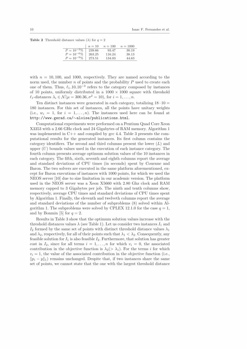
Table 1 and 2 present the values of threshold distances λ obtained fromequations (11) and (12) for q = 1 and q = 2, respectively, considering differentvalues of P and different number of points n.

Table 1 Threshold distance values (λ) for q = 1

n = 10 n = 100 n = 1000P = 10−3% 300.36 117.15 37.85P = 10−6% 329.93 145.68 47.79P = 10−9% 342.79 167.98 55.94

Eighteen different instance categories were generated based on the scenar-ios presented in Tables 1 and 2; nine for q = 1 and nine for q = 2. For theseinstance categories, the threshold distance values are taken from the valuespresented in Tables 1 and 2 plus a perturbation obtained from a normal dis-tribution with mean 0 and variance equal to 10, 5, and 2 for the instances


Table 2 Threshold distance values (λ) for q = 2

n = 10 n = 100 n = 1000P = 10−3% 239.66 93.47 30.19P = 10−6% 263.25 116.24 38.13P = 10−9% 273.51 134.03 44.63

with n = 10, 100, and 1000, respectively. They are named according to thenorm used, the number n of points and the probability P used to create eachone of them. Thus, ℓ1 10 10−3 refers to the category composed by instancesof 10 points, uniformly distributed in a 1000 × 1000 square with thresholdℓ1-distances λi ∈ N (µ = 300.36, σ2 = 10), for i = 1, . . . , n.

Ten distinct instances were generated in each category, totalizing 18 · 10 =180 instances. For this set of instances, all the points have unitary weights(i.e., wi = 1, for i = 1, . . . , n). The instances used here can be found athttp://www.gerad.ca/∼aloise/publications.html.

Computational experiments were performed on a Pentium Quad Core XeonX3353 with a 2.66 GHz clock and 24 Gigabytes of RAM memory. Algorithm 1was implemented in C++ and compiled by gcc 4.4. Table 3 presents the com-putational results for the generated instances. Its first column contains thecategory identifiers. The second and third columns present the lower (L) andupper (U) bounds values used in the execution of each instance category. Thefourth column presents average optimum solution values of the 10 instances ineach category. The fifth, sixth, seventh and eighth columns report the averageand standard deviations of CPU times (in seconds) spent by Couenne andBaron. The two solvers are executed in the same platform aforementioned, ex-cept for Baron executions of instances with 1000 points, for which we used theNEOS server [10] due to size limitation in our academic version. The platformused in the NEOS server was a Xeon X5660 with 2.80 Ghz clock and RAMmemory capped to 3 Gigabytes per job. The ninth and tenth columns show,respectively, average CPU times and standard deviations of CPU times spentby Algorithm 1. Finally, the eleventh and twelveth columns report the averageand standard deviations of the number of subproblems (8) solved within Al-gorithm 1. The subproblems were solved by CPLEX 12.1.0 for the case q = 1,and by Bonmin [5] for q = 2.

Results in Table 3 show that the optimum solution values increase with thethreshold distances values λ (see Table 1). Let us consider two instances I1 andI2 formed by the same set of points with distinct threshold distance values λ1

and λ2, respectively, for all of their points such that λ1 < λ2. Consequently, anyfeasible solution for I1 is also feasible I2. Furthermore, that solution has greatercost in I2, since for all terms i = 1, . . . , n for which vi = 0, the associatedcontribution in the objective function is λ2(> λ1). For the terms i for whichvi = 1, the value of the associated contribution in the objective function (i.e.,‖pi − y‖1) remains unchanged. Despite that, if two instances share the sameset of points, we cannot state that the one with the largest threshold distance

Title

Suppressed

Dueto

Excessiv

eLen

gth

11

Table 3 Computational results of Algorithm 1, Couenne and Baron over the 180 generated instances.

Couenne Baron Algorithm 1Category L U opt.value CPU time(s) std.dev. CPU time(s) std.dev. CPU time(s) std.dev. # subs std.dev.ℓ1 10 10−3 2 5 2199.25 5.95 7.17 38.84 76.11 0.43 0.27 97.6 29.56ℓ1 10 10−6 2 5 2389.11 7.90 10.52 35.04 68.49 0.49 0.21 120.4 26.75ℓ1 10 10−9 2 5 2471.41 7.12 9.52 34.35 67.00 0.58 0.13 136.0 23.99ℓ1 100 10−3 5 10 11140.50 40.88 9.82 244.18 154.89 4.67 1.71 1034.1 307.17ℓ1 100 10−6 5 10 13766.76 56.94 12.66 274.71 172.39 14.73 5.96 2825.8 495.58ℓ1 100 10−9 5 10 15787.32 74.82 22.55 453.34 306.70 28.70 11.99 4919.6 418.58ℓ1 1000 10−3 10 20 34207.28 2022.68 183.83 17703.40 7169.93 0.84 0.27 110.11 59.27ℓ1 1000 10−6 10 20 44037.39 3251.83 339.03 25896.00 1524.11 12.94 4.44 2737.8 1017.28ℓ1 1000 10−9 10 20 52088.12 5148.95 846.75 27645.66 2511.78 67.48 13.72 14621.6 2901.73

ℓ2 10 10−3 2 5 1874.70 1.83 0.96 6.90 10.87 4.06 4.55 99.0 28.42ℓ2 10 10−6 2 5 2026.11 1.88 0.67 1.55 1.14 5.97 7.96 116.0 26.02ℓ2 10 10−9 2 5 2090.42 1.85 0.78 1.59 0.92 6.20 6.53 127.8 30.45ℓ2 100 10−3 5 10 2199.25 66.85 31.10 92.34 19.67 104.31 51.29 1037.9 306.79ℓ2 100 10−6 5 10 2389.11 144.10 410.03 94.21 26.26 269.85 84.04 2828.4 538.19ℓ2 100 10−9 5 10 2471.41 379.02 334.88 90.80 24.78 542.75 169.91 4878.6 444.51ℓ2 1000 10−3 10 20 29971.70 3016.79 859.24 8266.79 917.73 2.58 0.84 88.6 53.78ℓ2 1000 10−6 10 20 37823.32 13916.58 3403.56 15898.89 2666.81 97.28 47.69 2654.8 991.75ℓ2 1000 10−9 10 20 44243.26 30583.92 16320.27 18040.20 4351.75 515.68 162.04 14459.3 2995.86


has the largest optimal solution value (the trivial case is an infeasible locationproblem with λ1, which becomes feasible by using λ2).

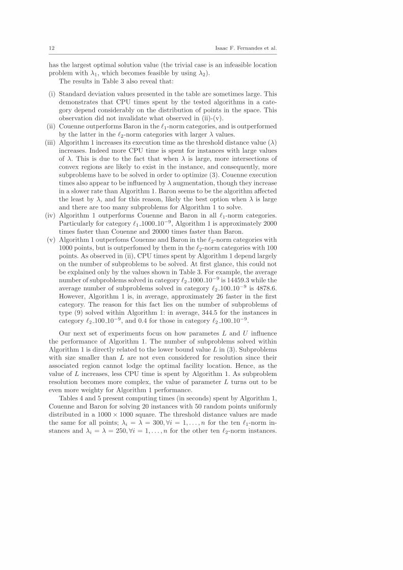
The results in Table 3 also reveal that:

(i) Standard deviation values presented in the table are sometimes large. Thisdemonstrates that CPU times spent by the tested algorithms in a cate-gory depend considerably on the distribution of points in the space. Thisobservation did not invalidate what observed in (ii)-(v).

(ii) Couenne outperforms Baron in the ℓ1-norm categories, and is outperformedby the latter in the ℓ2-norm categories with larger λ values.

(iii) Algorithm 1 increases its execution time as the threshold distance value (λ)increases. Indeed more CPU time is spent for instances with large valuesof λ. This is due to the fact that when λ is large, more intersections ofconvex regions are likely to exist in the instance, and consequently, moresubproblems have to be solved in order to optimize (3). Couenne executiontimes also appear to be influenced by λ augmentation, though they increasein a slower rate than Algorithm 1. Baron seems to be the algorithm affectedthe least by λ, and for this reason, likely the best option when λ is largeand there are too many subproblems for Algorithm 1 to solve.

(iv) Algorithm 1 outperforms Couenne and Baron in all ℓ1-norm categories.Particularly for category ℓ1 1000 10−9, Algorithm 1 is approximately 2000times faster than Couenne and 20000 times faster than Baron.

(v) Algorithm 1 outperfoms Couenne and Baron in the ℓ2-norm categories with1000 points, but is outperfomed by them in the ℓ2-norm categories with 100points. As observed in (ii), CPU times spent by Algorithm 1 depend largelyon the number of subproblems to be solved. At first glance, this could notbe explained only by the values shown in Table 3. For example, the averagenumber of subproblems solved in category ℓ2 1000 10−9 is 14459.3 while theaverage number of subproblems solved in category ℓ2 100 10−9 is 4878.6.However, Algorithm 1 is, in average, approximately 26 faster in the firstcategory. The reason for this fact lies on the number of subproblems oftype (9) solved within Algorithm 1: in average, 344.5 for the instances incategory ℓ2 100 10−9, and 0.4 for those in category ℓ2 100 10−9.

Our next set of experiments focus on how parametes L and U influencethe performance of Algorithm 1. The number of subproblems solved withinAlgorithm 1 is directly related to the lower bound value L in (3). Subproblemswith size smaller than L are not even considered for resolution since theirassociated region cannot lodge the optimal facility location. Hence, as thevalue of L increases, less CPU time is spent by Algorithm 1. As subproblemresolution becomes more complex, the value of parameter L turns out to beeven more weighty for Algorithm 1 performance.

Tables 4 and 5 present computing times (in seconds) spent by Algorithm 1,Couenne and Baron for solving 20 instances with 50 random points uniformlydistributed in a 1000 × 1000 square. The threshold distance values are madethe same for all points; λi = λ = 300, ∀i = 1, . . . , n for the ten ℓ1-norm in-stances and λi = λ = 250, ∀i = 1, . . . , n for the other ten ℓ2-norm instances.


The tables report, varying only the lower bound value L (in this set of exper-iments U = +∞), the average and the standard deviation of the CPU timespent by Algorithm 1, Couenne and Baron on solving the generated instances.Regarding Algorithm 1, the tables also report the average and the standarddeviation of the number of subproblems solved.

Table 4 CPU times (in seconds) of Algorithm 1, Couenne and Baron as a function of lowerbound in ten ℓ1-norm distinct instances with 50 random points

Algorithm 1 Couenne BaronL CPU time(s) std.dev. # subs std.dev. CPU time(s) std.dev. CPU time(s) std.dev.5 8.57 1.67 3651.9 399.47 45.14 15.82 116.481 119.90

10 3.29 1.32 1374.0 544.96 41.87 7.64 125.83 120.5715 0.35 0.73 133.2 263.26 26.08 9.91 35.86 16.83

Table 5 CPU times (in seconds) of Algorithm 1, Couenne and Baron as a function of lowerbound in ten ℓ2-norm distinct instances with 50 random points

Algorithm 1 Couenne BaronL CPU time(s) std.dev. # subs std.dev. CPU time(s) std.dev. CPU time(s) std.dev.5 392.80 116.01 3998.0 381.78 319.61 295.17 33.49 12.99

10 84.67 55.96 1799.0 586.56 264.92 299.82 33.85 12.8915 5.38 10.60 224.6 313.11 105.25 224.00 30.10 8.39

We notice from Tables 4 and 5 that Algorithm 1 improves considerablyits performance as L augments and the number of subproblems decreases.The same is also observed for Couenne, though in a smaller rate. For thisexperiment, Algorithm 1 is clearly the best approach for the ℓ1 instances,but became the best option for the ℓ2 instances only after L was increasedto 15 and the number of subproblems decreased enough. The reason for thisperformance difference while solving ℓ1 and ℓ2-norm instances relies on thecomplexity of the subproblems of type (8): linear for ℓ1-norm instances andconvex non-linear for ℓ2-norm ones. Furthermore, Baron does not appear to beinfluenced by L as much as the other algorithms are. For the ℓ2-norm instanceswith L = 5, 10, Baron outperforms Algorithm 1 and Couenne.

The last set of experiments addresses the influence of parameter U on Al-gorithm 1 performance. For that purpose, the algorithm was used to solve thesame 20 instances of the last experiment, but this time for different combina-tions of L and U values. Tables 6 and 7 report, the average computing times,and its standard deviations, spent by Algorithm 1. Moreover, the average andstandard deviation of the number of subproblems of type (8) and (9) solvedwithin the algorithm are presented. The tables also present the average and


the standard deviation of the CPU times spent by Couenne and Baron onsolving (3) for the 10 instances of each norm.

From these last results, we notice that the performance of Algorithm 1 isimproved as U augments. Whenever the size of a subproblem is smaller or equalto U , a subproblem of type (9) is solved instead of a more difficult subproblemof type (8). For example, when U increases from 15 to 20 in Table 7, the averagenumber of subproblems of type (8) that becomes solvable by model (9) withinAlgorithm 1 is 135.1−4.1 = 131.1. Consequently, the average CPU time spentby the algorithm drops from 145.49 to 86.55 seconds.

Furthermore, we observe from Table 7 that Algorithm 1 always outperformsCouenne, but is outperformed by Baron with parameters L = 10, U = 15and L = 10, U = 20. Indeed if the total number of subproblems is large, thedecomposition approach of Algorithm 1 may not be the best strategy to choose.Although the subproblems solved by Algorithm 1 are smaller and require lesscomputing time, they may be too numerous so that the total time spent onsolving all them is greater than solving the original problem (3) directly. Thisfact was not observed in the results of Table 6 because the ℓ1-subproblems areeasier to solve than those in the ℓ2 norm.

Finally, it is worthy mentioning that standard deviations of computingtimes and the number of subproblems for Algorithm 1 and Couenne are dueto the presence of instances with different hardness degrees. In particular,one instance was noticed to be much harder than the others for Algorithm 1and Couenne. If the same was removed from the experiment with ℓ2-norminstances, the average CPU time of Algorithm 1 would be 85.61 seconds withparameters L = 10 and L = 15 (std.dev. 57.34), 68.49 seconds with L = 10 andU = 20 (std.dev. 54.56), and 1.87 seconds with L = 15 and U = 20 (std.dev.2.08). For Couenne, the corresponding average CPU times would be: 221.39(std.dev. 161.95), 231.36 (std.dev 192.00), and 28.43 seconds (std.dev. 24.94).This demonstrates that the points distribution in the space plays a key rolein the performance of our algorithm. Indeed it directly influences the numberand the type of the subproblems to be solved.

4.1 Application to a real-life problem

We report computational results obtained on a real-life problem provided bythe Natal Police Department in Brazil. The data consists of 586 sites in Natal,Brazil where criminal activities were recorded in the period from 01/01/09 to09/30/2009. It contains, for each site, its coordinates in UTM scale, which areapproximated to the Euclidean space, and the number of recorded crimes inthe analyzed period, which are used to weight the demand of that site for apolice station close-by. The objective for this problem is to locate a new policestation close to where the police demand is high, but also respecting lowercapacity constraints which are useful to better distribute the police coverageover the city.

Title

Suppressed

Dueto

Excessiv

eLen

gth

15

Table 6 CPU times (in seconds) of Algorithm 1, Couenne and Baron as a function of lower and upper bounds in ten ℓ1-norm distinct instances with50 random points

Algorithm 1 Couenne BaronL U CPU time(s) std.dev. # subs(6) std.dev. # subs(7) std.dev. CPU time(s) std.dev. CPU time(s) std.dev.10 15 2.32 2.47 1374.0 544.96 76.2 193.29 63.19 24.69 63.19 24.6910 20 1.58 0.68 1374.0 544.96 0.8 2.52 47.22 17.27 130.50 114.9715 20 0.18 0.37 133.2 263.26 0.8 2.52 27.92 10.45 40.26 19.89

Table 7 CPU times (in seconds) of Algorithm 1, Couenne and Baron as a function of lower and upper bounds in ten ℓ2-norm distinct instances with50 random points

Algorithm 1 Couenne BaronL U CPU time(s) std.dev. # subs(6) std.dev. # subs(7) std.dev. CPU time(s) std.dev. CPU time(s) std.dev.10 15 145.49 166.60 1799.0 586.56 135.1 254.10 658.99 1313.73 35.18 13.0210 20 86.55 59.07 1799.0 586.56 4.1 12.96 431.68 579.25 35.18 9.2715 20 7.13 16.06 224.6 313.11 4.1 12.96 136.64 332.98 26.83 9.74


Our tests used λ = 1 kilometer (estimated in [17]) in ℓ1-norm for all sites.Besides, no upper bound capacity U is used due to the nature of the applica-tion. Two different scenarios were tested by varying the value of L: scenarioA uses L = 10, and scenario B uses L = 25. We solved the correspondingLDMPSC problem using Algorithm 1, Couenne and Baron. The optimal so-lutions in scenarios A and B are shown in Figure 2, where the problem isgeographically represented.

Fig. 2 Geographic distribution of criminal records in the city of Natal, Brazil from01/01/2009 to 09/30/2009. The size of the plotted points is proportional to the numberof criminal records of the corresponding site. Thus, the smallest points represent sites wherethe number of criminal records was between 0 and 50, and the largest points represent siteswhere the number of records was greater than 1000. The optimal locations for positioninga police unity in scenarios A and B are represented by a yellow and a red star, respectively.

Algorithm 1 outperforms Couenne and Baron in both scenarios. Algo-rithm 1 solves scenario A in 102.30 seconds, Couenne is not able to solveit within 1 hour, and Baron solves it in 1614.38. Regarding scenario B, Al-gorithm 1 solves it in 10.72 seconds, Couenne is again not able to solve theproblem within 1 hour, and Baron solves it in 1715.37.

5 Conclusions

The introduction of side constraints while locating a facility in the plane withlimited distances may serve to justify its installation or to describe service


limitations. Our work extends that of Drezner, Mehrez and Wesolowsky [13],adapting it to the presence of side constraints. This approach leads to sub-problems having products of the continuous location variable with assignmentbinary variables. The subproblem model is then reformulated in order to easeits resolution. In summary, the performance of the presented algorithm is in-fluenced by:

(i) the complexity of the subproblems - e.g. subproblem (8) is a MILP if ℓ1-distances are used, and a non-differentiable convex MINLP for ℓ2-distances;

(ii) the number of subproblems to be solved - this is linked with the thresholddistances values;

(iii) the lower bound of service - this allows to disregard the resolution of somesubproblems;

(iv) the upper bound of service - easier subproblems to solve due to removinginteger decision variables.

Finally, it is important to remark that the proposed algorithm can bestraightforwardly parallelized, since no dependence exists among the solvedsubproblems.

Acknowledgements We are thankful to Andre Morais Gurgel and the Natal Police De-partment for providing us the data for the real instance. We also thank two anonymousreferees for insightful remarks.

References

1. Aloise, D., Hansen P., Liberti, L.: An improved column generation algorithm for minimumsum-of-squares clustering, Mathematical Programming, 131, 195–220 (2012).

2. Belotti, P., Lee J., Liberti L., Margot F., Wachter A.: Branching and bounds tighten-ing techniques for non-convex MINLP, Optimization Methods and Software, 24, 597–634(2009).

3. Berman, O., Drezner, Z., Krass, D.: Generalized coverage: New developments in coveringlocation models, Computers and Operations Research, 37, 1675–1687 (2010).

4. Brimberg, J., Chen, R., Chen D.: Accelerating convergence in the Fermat-Weber locationproblem. Operations Research Letters, 22, 151–157 (1998).

5. Bonami, P., Lee J.: BONMIN user’s manual. Technical report, IBM Corporation (2007).6. P. Bonami, L. Biegler, A.R. Conn, G. Cornuejols, I.E. Grossmann, C.D. Laird, J. Lee,A. Lodi, F. Margot, N. Sawaya, A. Wachter: An algorithmic framework for convex mixedinteger nonlinear programs, Discrete Optimization, 5, 186–204 (2008).

7. Boyd, S., Vandenberghe, L.: Convex Optimization, Cambridge University Press, Cam-bridge 2004.

8. Church R., ReVelle C.: The maximal covering location problem. Papers of the RegionalScience Association, 32, 101–118 (1974).

9. Church, R., Roberts K.L.: Generalized coverage models and public facility location. Pa-pers of the Regional Science Association, 53, 117–135 (1983).

10. Czyzyk, J., Mesnier, M., More, J.: The NEOS Server. IEEE Journal on ComputationalScience and Engineering, 5, 68–75 (1998).

11. de Berg, M., van Krefeld, M., Overmars, M., Schwarzkopf, O.: Computational Geometry:Algorithms and Applications, Springer (1997).

12. Drezner Z., Wesolowsky, G.O.: A maximin location problem with maximum distanceconstraints, AIIE Transactions, 12, 249–252 (1980).


13. Drezner Z., Mehrez A., Wesolowsky, G.O.: The facility location problem with limiteddistances. Transportation Science, 25, 183–187 (1991).

14. Drezner, Z., Hamacher H.W.: Facility Location: Applications and Theory. Springer(2004).

15. Drezner, Z., Wesolowsky, G.O., Drezner, T.: The gradual covering problem. Naval Re-search Logistics, 51, 841–855 (2004).

16. Fekete, S.P., Mitchell, J.S.B, Beurer, K.: On the continuous Fermat-Weber problem.Operations Research, 53, 61–76 (2005).

17. A.M. Gurgel: Melhoria da seguranca publica: Uma proposta para a alocacao de unidadespoliciais utilizando o modelo das p-medianas e do caixeiro viajante. M.Sc. dissertation.Universidade Federal do Rio Grande do Norte (2010).

18. Hansen, P., Mladenovic, N., Taillard, E.: Heuristic solution of the multisource Weberproblem as a image-median problem”. Operations Research Letters, 22, 55–62 (1998).

19. Liberti, L.: Writing global optimization software, in Liberti, L., Maculan, N. (eds.),Global Optimization: from Theory to Implementation, 211-262, Springer, Berlin (2006).

20. Liberti, L.: Reformulations in Mathematical Programming: Definitions and systematics.RAIRO-RO, 43, 55–86 (2009).

21. Pirkul, H., Schilling, D.A.: The maximal covering location problem with capacities ontotal workload. Management Science, 37, 233–248 (1991).

22. Schilling, D.A., Jayaraman V., Barkhi, R.: A review of covering problems in facilitylocation. Location Science, 1, 25–55 (1993).

23. Smith, E., Pantelides, C.: A symbolic reformulation/spatial branch-and-bound algo-rithm for the global optimisation of nonconvex MINLPs, Computers & Chemical Engi-neering, 23, 457-478 (1999).

24. Smith, H.K., Laporte, G., Harper, P.R.: Locational analysis: highlights of growth tomaturity. Journal of the Operational Research Society, 60, 140–148 (2009).

25. Tawarmalani, M., Sahinidis, N.V.: A polyhedral branch-and-cut approach to globaloptimization. Mathematical Programming, 103, 225–249 (2005).

26. Wesolowsky, G.O.: The Weber problem: history and perspectives. Location Science, 1,5–23 (1993).

on the weber facility location problem with limited

Documents