one‐ and two‐dimensional modelling of overland flow in

HYDROLOGICAL PROCESSESHydrol. Process. 20, 1027–1046 (2006)Published online in Wiley InterScience (www.interscience.wiley.com). DOI: 10.1002/hyp.5922

One- and two-dimensional modelling of overland flow insemiarid shrubland, Jornada basin, New Mexico

David A. Howes,1* Athol D. Abrahams2 and E. Bruce Pitman3

1 Compliance Services International, 7501 Bridgeport Way West, Lakewood, WA 98499, USA2 Department of Geography, University at Buffalo, The State University of New York, Buffalo, NY 14261, USA

3 Department of Mathematics, University at Buffalo, The State University of New York, 244 Mathematics Building, Buffalo, NY 14260, USA

Abstract:

Two distributed parameter models, a one-dimensional (1D) model and a two-dimensional (2D) model, are developedto simulate overland flow in two small semiarid shrubland watersheds in the Jornada basin, southern New Mexico. Themodels are event-based and represent each watershed by an array of 1-m2 cells, in which the cell size is approximatelyequal to the average area of the shrubs.

Each model uses only six parameters, for which values are obtained from field surveys and rainfall simulationexperiments. In the 1D model, flow volumes through a fixed network are computed by a simple finite-differencesolution to the 1D kinematic wave equation. In the 2D model, flow directions and volumes are computed by asecond-order predictor–corrector finite-difference solution to the 2D kinematic wave equation, in which flow routingis implicit and may vary in response to flow conditions.

The models are compared in terms of the runoff hydrograph and the spatial distribution of runoff. The simulationresults suggest that both the 1D and the 2D models have much to offer as tools for the large-scale study of overlandflow. Because it is based on a fixed flow network, the 1D model is better suited to the study of runoff due to individualrainfall events, whereas the 2D model may, with further development, be used to study both runoff and erosion duringmultiple rainfall events in which the dynamic nature of the terrain becomes an important consideration. Copyright 2006 John Wiley & Sons, Ltd.

KEY WORDS runoff; overland flow; infiltration; drainage basin; hydrology

INTRODUCTION

Distributed parameter modelling is the most widely used method of modelling runoff in semiarid environments(e.g. Zhang and Cundy, 1989; Goodrich et al., 1991; Moore and Grayson, 1991; Vertessy et al., 1993; Flanaganand Nearing, 1995; Smith et al., 1995). This approach provides a detailed representation of the watershed andan accurate description of the runoff processes using physically based relationships. A watershed is representedas a set of spatial (distributed) elements and the model simulates (1) the hydrologic processes operating withineach element (i.e. the conversion of rainfall to runoff), and (2) the flow of water between the elements (i.e.surface runoff).

Distributed parameter models are classified according to (1) the description of the runoff processes and(2) the dimensionality of the flow description. In the first case, models are classified as deterministic, stochastic,or mixed, depending on the degree of certainty with which the runoff processes are described in the model(Singh, 1996). In the second case, models are classified as either one-dimensional (1D) or two-dimensional(2D). For the simulation of runoff in very small watersheds, both types of model typically employ thekinematic wave approximation to the Saint Venant flow equations. This method involves numerically solvingthe continuity or mass balance equation using a uniform flow approximation to compute flow velocity.

* Correspondence to: David A. Howes, Compliance Services International, 7501 Bridgeport Way West, Lakewood, WA 98499, USA.E-mail: [email protected]

Received 23 April 2003Copyright 2006 John Wiley & Sons, Ltd. Accepted 19 January 2005

1028 D. A. HOWES, A. D. ABRAHAMS AND E. B. PITMAN

1D models

1D runoff models are based on the assumption that runoff from a watershed can be treated as a set of 1Dflows and that these flows may be integrated to provide a simulated hydrograph at the outlet of the watershed.This concept is generally implemented in a distributed parameter model in one of two ways. The first involvesdefining the model elements such that they form cascades, whereas the second involves the use of a flowrouting algorithm to determine a single outflow direction for each element based on the local topography. Thefirst approach is illustrated by THALES (Grayson et al., 1992a) and TOPOG (Vertessy et al., 1993), whichuse the ‘stream-tubes’ concept of Onstad and Brakensiek (1968), and by KINEROS (Smith et al., 1995) andWEPP (Flanagan and Nearing, 1995), which represent hillslopes and channels by cascading planes.

The second 1D approach is illustrated by the model of Scoging et al. (1992). In this model, a hillslopeor watershed is represented as a grid of square cells, and a flow network is defined using a simple routingalgorithm, which allows flow to occur from each cell to one of its eight neighbours. The volume of flowthrough the network is computed by solving the 1D kinematic wave equation at the centre of each cell.Scoging et al. (1992) applied this model to a large runoff plot (35 m long and 18 m wide) on a shrublandhillslope at Walnut Gulch, and Parsons et al. (1997) applied a modified version of the model to another largerunoff plot (29 m long and 18 m wide) on a grassland hillslope at Walnut Gulch. By comparing simulatedhydrographs with observed hydrographs, the two studies showed that the model worked well for cell sizesranging from 0Ð5 to 10 m2.

2D models

In contrast to the 1D models described above, 2D models route flow implicitly and are mathematically morecomplex. However, according to Zhang and Cundy (1989), 2D models simulate the spatial distribution ofoverland flow more realistically and with greater accuracy than 1D models do. Goodrich et al. (1991) applieda 2D runoff model based on a set of triangular elements to a portion of the Lucky Hills watershed at WalnutGulch and compared the model results with hydrographs generated by KINEROS. The two models producedsimilar results. Gao et al. (1993) applied a 2D runoff model based on a regular grid spatial structure to thesame watershed. Their model was applied without calibration and the results were found to match measuredrunoff data reasonably well.

Modelling overland flow in the Jornada shrubland

The focus of the present study is on the modelling of runoff processes on the creosotebush (Larreatridentata) shrubland in the Jornada basin, southern New Mexico. This study is part of the Jornada basinLong-Term Ecological Research (LTER) project, which is concerned with the causes and consequences of thewidespread replacement of grassland by shrubland in the American Southwest.

Studies concerned with the supply of water to shrubs tend to focus on the role of interception and stemflow(e.g. Navar and Bryan, 1990; Martinez-Meza and Whitford, 1996; Abrahams et al., 2005). Furthermore, plantgrowth models developed by Reynolds et al. (1997) to simulate the evolution of shrubland ecosystems arebased on the assumption that all of the water reaching a shrub originates as rain falling directly onto the shrub.However, the lateral redistribution of water by overland flow is widely recognized as being critical to plantproduction of desert ecosystems (Schlesinger and Jones, 1984; Noy-Meir, 1985). On shrubland hillslopes,most shrubs reside on microtopographic mounds a few centimetres high. These cause overland flow in thebare intershrub areas to concentrate in flowpaths, where it diverges and converges around the shrubs in acomplex reticular pattern. Nonetheless, significant quantities of water flow onto and off shrub mounds, bothadding to and subtracting from the supply of water and nutrients to individual shrubs. These processes havereceived little attention, in large part due to the lack of a suitable model to simulate overland flow at thisscale.

Howes and Abrahams (2003) developed a 2D model to simulate runon at the scale of the individual shrubin two small watersheds in the creosotebush shrubland of the Jornada basin. This 2D model is mathematically

Copyright 2006 John Wiley & Sons, Ltd. Hydrol. Process. 20, 1027–1046 (2006)

MODELLING OVERLAND FLOW 1029

quite complex. Consequently, in this study a 1D model is developed that is mathematically simpler than the2D model. This model is applied to simulate the runoff in the same two watersheds and the performanceof the models is then compared in terms of both the runoff hydrograph and the spatial pattern of overlandflow.

In order to simulate overland flow accurately in the Jornada shrubland, the 1D and 2D models were designedto satisfy the following requirements:

1. The model elements must be small enough to discriminate between shrub and intershrub areas.2. The model must be able to represent accurately the divergence and convergence of flow around individual

shrubs.3. The model should contain the optimum number of parameters to describe the runoff processes accurately,

but not in excessive detail.4. Where possible, the model parameter values should be obtainable from field experiments conducted at the

same scale as the model elements.

MODEL DEVELOPMENT

Kinematic wave approximation

The 1D and 2D models are based on the kinematic wave approximation to the Saint Venant flow equations(de Saint Venant, 1871; Ponce, 1991)

∂h

∂tC ∂q

∂xD r � f 1D �1�

∂h

∂tC ∂q

∂xC ∂q

∂yD r � f 2D �2�

where h (cm) is the flow depth, t (h) is the time, x and y (cm) are the space increments, r (cm h�1) is therainfall rate, f (cm h�1) is the infiltration capacity, and q (cm2 h�1) is the unit discharge, which is computedas

q D vh �3�

where v (cm s�1) is the flow velocity. Inasmuch as the kinematic wave approximation is based on theassumption that changes in momentum in overland flow are negligible compared with both the gravitationalforce (which promotes flow) and the frictional forces (which transmit the frictional effects of the surface intothe flow) (Baird, 1997), v may be calculated using a uniform flow approximation. Thus, gradually varied,non-uniform, free-surface flow may be visualized as a succession of steady uniform flows (Chow, 1959;Ponce, 1991).

Uniform flow velocity

The 1D and 2D models employ the Darcy–Weisbach flow equation

v D√

8ghs

ff�4�

where g (cm s�2) is the acceleration due to gravity, s is the slope, and ff is the friction factor.In the kinematic wave approximation, the relationship between q and h is known as the kinematic

approximation to the momentum equation (Sherman and Singh, 1976) or the rating equation. This equationhas the form

q D ˛hm �5�



where ˛ (cm2�m h�1) is the kinematic wave friction relationship parameter and m is the slope-frictioncoefficient. When v is computed using the Darcy–Weisbach equation and s and ff are constant, then ˛and m are both constants and their values can be obtained from Equation (4) as follows:

v D√

8ghs

ffD ˛h0Ð5 �6�

where ˛ D p8gs/ff . Therefore, from Equation (3)

q D vh D ˛h1Ð5 �7�

Thus, m in Equation (5) is equal to 1Ð5.

Infiltration

Infiltration is described in the model using the storage-based Smith–Parlange equation (Smith and Parlange,1978; Woolhiser et al., 1990)

f D Ks eF/B

eF/B � 1f > 0 �8�

where f (cm h�1) is the infiltration capacity, Ks (cm h�1) is the saturated hydraulic conductivity, F (cm) isthe infiltrated depth, and B (cm) is a soil storage parameter (Freeze, 1980) defined by

B D S2

2Ks�9�

where S (cm h�0Ð5) is the sorptivity accounting for both capillary suction and initial conditions.If the soil properties are the same throughout the watershed and all points receive the same amount of

rainfall, then ponding occurs at all points simultaneously. However, most soil properties are highly variableover short distances (e.g. Nielsen et al., 1973; Springer and Cundy, 1987), and this spatial variability maygive rise to runon infiltration. Runon infiltration occurs when runoff generated in an upslope area encountersa downslope area where ponding has not occurred. In the latter area, the rainfall excess is still negative, sothe soil still has infiltration capacity to satisfy. Some or all of this unsatisfied capacity may be filled by runon.The effect of runon infiltration is to increase the infiltrated depth, and thus accelerate ponding, causing runoffto occur earlier than it otherwise would (Scoging et al., 1992).

Using Equation (8) and allowing for runon infiltration, the infiltration rate i (cm s�1) is computed aseither

i D qr C r for f > qr C r �10�

ori D f for f � qr C r

where qr (cm h�1) is the runon per unit surface area.

1D MODEL

Numerical solution scheme

In the 1D runoff model, a first-order 1D finite-difference scheme is used to solve the 1D kinematic waveequation (Equation (1)). The finite-difference form of this equation is

htCti � ht

i

tC qt

i � qti�x

xD ext

i �11�



where subscript i is a spatial node on the flowpath, x is the space increment, and ex D r � f. This schemeis known as a backward-space scheme because the space differencing occurs backwards with respect to thedirection of flow (i.e. upslope).

Rearranging Equation (11), and solving for h at the next time step gives

htCti D ht

i � t

x�qt

i � qti�x� C ext

i �12�

Stability

The numerical solution to the 1D kinematic wave equation can be prevented from becoming unstable bythe use of two stability constraints, both of which must be satisfied. The first of these is the Courant condition,a stability measure relating u, t, and x, which refers to the left side of Equation (1).

The Courant condition states that the scheme will remain stable as long as

ut

x� 1 �13�

The left side of this equation is referred to as the Courant number.In the 1D numerical solution scheme, t can be varied at each time step in response to instability, and also

as a means of improving efficiency. Should the Courant number exceed unity, the value of t is reduced andthe value of h recalculated.

The efficiency of the numerical scheme can also be improved by choosing as large a value of t as possiblewhile ensuring that the value used will not cause the scheme to become unstable. A suitable value of t canbe obtained by rearranging Equation (13) to give

t D Cx

u�14�

where C is the Courant coefficient, and 0 < C < 1.Using Equation (14), t will vary with the flow conditions. If conditions are changing rapidly, t will be

very small, but if conditions are changing more slowly, t will have a larger value. Thus, when time stepsare selected according to the Courant condition, the numerical scheme is able to respond to the variabilitypresent in the analytical solution.

The value of C is generally fixed, but this is not required. In many applications using the Courant condition,C D 0Ð9 is an appropriate choice. However, the value of t provided by Equation (14) may be too largein situations where flow conditions change extremely rapidly, causing the solution scheme to become unstable.As long as the Courant condition is checked at the end of each time step, this situation can be addressedby recalculating h using a smaller t. If the estimates of t are consistently too large, then a smaller valueof C can be used in the scheme to reduce the number of times that h must be recalculated. In testing themodels for the Jornada shrubland, it was found that C had to be as low as 0Ð1. This is because the velocity ofoverland flow in the shrubland can be high (in excess of 1Ð3 m s�1) and can change rapidly due to a numberof factors, including the convergence and divergence of flow around shrub mounds and sudden variations inrainfall intensity during summer thunderstorms.

The second stability constraint applies to the source term (the right-hand side of Equation (1)). In general,if A is the magnitude of the source term, then the numerical scheme will be stable as long as

t <1

A�15�

As with the Courant condition, problems may arise if conditions change rapidly. Therefore, requiring that

t <0Ð1A

�16�

is more reliable when modelling highly variable flow conditions typical of the Jornada shrubland.



Flow network

For the 1D model, flow networks are computed using the algorithm of Tarboton (1997). This algorithmwas selected (1) because of its ability to represent effectively the diverging and converging flowpaths of theJornada shrubland and (2) because it is a robust procedure which is based on a simple grid structure and isrelatively insensitive to grid orientation.

The Tarboton algorithm takes as input a digital elevation model (DEM) and, for every cell in theDEM, calculates a flow vector for each of eight triangular facets radiating from the centre of the cell.The steepest downslope vector from all eight facets is taken as the flow vector for the cell. Flow is thenapportioned between a maximum of two downslope cells according to a procedure described in Tarboton(1997).

Since it includes only one space dimension, the 1D kinematic wave equation applies to flow along a 1Dflowpath, which implies that any point along the flowpath can have only one inflow and one outflow. However,Scoging et al. (1992) and Parsons et al. (1997) showed that it is acceptable to treat the inflow to a spatialnode as the sum of several inflows and also to divide the outflow from a spatial node between a numberof cells. The 1D numerical scheme may, therefore, be used to compute the flow depth at each node in thediverging and converging flow network produced using the Tarboton algorithm.

Initial and boundary conditions

At the beginning of a simulated rainstorm, the value of h is set to zero at all nodes in the flow network,and the antecedent moisture is specified by assigning an initial value to F in the Smith–Parlange equation(Equation (8)).

2D MODEL

Numerical solution scheme

The spatial and temporal variations in flow depth are simulated in the model by numerical solution ofthe 2D kinematic wave equation (Equation (2)) using a second-order accurate predictor–corrector finite-difference scheme developed by Davis (1988). The Davis algorithm was originally designed for problemsin computational fluid dynamics and provides greater spatial and temporal accuracy than the 1D numericalschemes used previously in modelling overland flow (e.g. Scoging et al., 1992; Parsons et al., 1997). Theability of the algorithm to capture nonlinear shocks and expansion waves smoothly and accurately makes itwell suited to modelling the rapidly changing flow conditions typical of the Jornada shrubland. The modeldeveloped by Howes and Abrahams (2003) represents the first application of the Davis algorithm to modellingoverland flow.

The Davis algorithm can be summarized as follows. For each cell in the model grid, the flow depth iscalculated at each time step by taking into account the flows between the cell and each of the eight neighbouringcells. Flows in the cardinal directions are calculated explicitly, whereas those between the cell and its diagonalneighbours are calculated implicitly. A simplified version of the equations underlying the algorithm is providedbelow. The reader is referred to Davis (1988) for further details. The simplified numerical scheme discussedbelow (Equation (19)) is not stable in its own right, but it is made stable by minor modifications included inthe Davis scheme.

Second-order accuracy in the spatial dimensions is obtained using centre-differencing. With the value ofthe source term �r � f� set to zero, Equation (2) can be expressed as

htCti,j � ht

i,j

tC qt

iCx,j � qti�x,j

2xC qt

i,jCy � qti,j�y

2yD 0 �17�



If the flow velocity in the x direction is denoted by a and that in the y direction is denoted by b usingEquation (3), then Equation (17) can be rewritten as

htCti,j � ht

i,j

tC a

2x

(ht

iCx,j � hti�x,j

)C b

2y

(ht

i,jCy � hti,j�y

)D 0 �18�

which can be solved for htCti,j to give

htCti,j D ht

i,j � at

2x�ht

iC1,j � hti�1,j� � b

t

2y�ht

i,jC1 � hti,j�1� �19�

Second-order accuracy in space is obtained using the midpoint rule in which h for a cell is computed in twosteps: at the midpoint of a given time step (the predictor step) and at the end of the time step (the correctorstep).

In the predictor step, h is estimated for each of the four cardinal neighbours of a cell, and these midtimevalues are used to compute h for the cell in the corrector step:

htCti,j D ht

i,j � at

2x�htCt/2

iC1,j � htCt/2i�1,j � � b

t

2y�htCt/2

i,jC1 � htCt/2i,j�1 � �20�

Thus, the calculation of htCti,j takes into account not only the components of flow along the axes, but also

the components of flow from the diagonal cells (i � 1, j C 1), (i C 1, j C 1), (i C 1, j � 1) and (i � 1, j � 1)through the calculation of the midtime h values in the predictor step. As for the 1D model, instability of thenumerical solution scheme is avoided by checking the Courant condition (Equation (13)) and the source termstability measure (Equation (16)) at the end of each time step and, if necessary, recomputing the h values forthe time step using a new time increment.

Initial and boundary conditions

The value of h is set to zero in all cells at the beginning of a simulation run, and the antecedent moistureis specified by assigning an initial value to F in the Smith–Parlange equation (Equation (8)). At the end ofeach time step during a model run, h is set to zero in all cells along the boundary of the model grid. In otherwords, the boundary cells act as permanent sinks. In general, this procedure is likely to have a negligibleeffect on the simulation of runoff in a watershed as long as the boundary cells are several metres from thewatershed boundary.

PARAMETERIZATION

Parameterization and calibration of physically based distributed runoff models have been the subject of muchdiscussion. This discussion has centred on the appropriate number of parameters to be used in such modelsand, in particular, on the number of parameters that require adjustment during calibration (e.g. Beven, 1989;Grayson et al., 1992b; Refsgaard, 1997). In general, as the number of parameters in a model increases, sotoo does the degree of interdependence between the parameters and, as a consequence, the chance of error.Additionally, as the number of parameters requiring adjustment during calibration increases, the greater isthe likelihood that the model output will not be a unique and accurate representation of the runoff process(Beven, 1989). These potential problems can be avoided by adherence to the following recommendations(Beven, 1989; Refsgaard and Storm, 1996; Refsgaard, 1997):

1. The number of parameters should be kept to a minimum while retaining the ability to represent the runoffprocesses accurately.



2. Values for as many of the parameters as possible should be determined from field data.3. The parameter values obtained from field experiments should be collected at the same scale as the model

elements to which they will be assigned.

In accordance with the first of these recommendations, the number of parameters employed in the 1D and2D runoff models was limited to six. Recommendations 1 and 2 are discussed in the following sections, whichdescribe the study watersheds and the spatial representation of these watersheds.

Study watersheds

The 1D and 2D models are parameterized for two small watersheds located in the creosotebush shrublandat the foot of Mount Summerford on the west side of the Jornada basin. The two watersheds differ slightly interms of their relief, surface properties, and the nature of the shrubs. These differences, however, are typicalof the variation across the creosotebush shrubland at Jornada. The watersheds are referred to as the north andsouth watersheds.

The north watershed (Figure 1), which has an area of 775 m2, lies ¾750 m downslope from MountSummerford. The shrubs in this watershed have an average height of 1Ð34 m and average canopy diameterof 1Ð59 m. Apart from occasional small forbs, vegetation is generally absent from the intershrub areas. Thesoil underlying the shrub and intershrub surfaces is a Typic Haplargid loamy sand (Schlesinger et al., 1999);the rills have sandy beds that, like the loamy sand, have a gravel content of <5% (by weight).

Figure 1. Map of the north watershed showing 5 cm contours, rills, and shrubs



All of the shrubs in the north watershed are underlain by the same type of soil, but this soil may bebare, covered by grass (Muhlenbergia porteri ), or covered by litter. The presence of vegetation or litterincreases the friction encountered by water flowing under the shrubs. This increased friction causes a reductionin flow velocity, thus increasing the likelihood that the water will infiltrate rather than run off into thesurrounding intershrub area. In addition, sub-canopy vegetation may enhance infiltration by increasing soilorganic matter and macroporosity through root decomposition and faunal activity (Abrahams et al., 2005).Since the differences in ground cover affect the amount of runoff in the watershed, it was necessary todistinguish between the three surface types in the modelling.

The south watershed (Figure 2), which has an area of 889 m2, is situated ¾1Ð2 km southeast of the northwatershed. Like the north watershed, it is located on Typic Haplargid soils (Schlesinger et al., 1999) but has amore incised rill network. The creosotebush in this watershed have an average height of 0Ð89 m and averagecanopy diameter of 0Ð92 m. Both the shrub mounds and intershrub areas are bare and consist of loamy sand,and the rill beds consist of sand. In contrast to the north watershed, gravel constitutes 30% of the rill andintershrub soils, and 5% of the shrub soil.

As shown in Table I, the parameter values for the north and south watersheds were acquired from watershedsurveys, watershed monitoring, and rainfall simulation experiments. The procedures used to obtain the datafor s, r Ks, B, Fi, and ff are described in detail in Howes and Abrahams (2003) and, therefore, will not bediscussed here.

Spatial representation of the watersheds

For the purpose of the modelling, each watershed is represented by a grid of 1 m2 cells. This guaranteesthat, apart from the creation of the 1D flow network, the parameterization process is virtually identical for the

Figure 2. Map of the south watershed showing 5 cm contours, rills, and shrubs



Table I. Model parameters and the source of their values

Parameter Symbol Source

Slope s DEM based on field surveyRainfall r Tipping-bucket rain gauge attached to data loggerSaturated hydraulic conductivity Ks Rainfall simulation experimentsSoil storage parameter B Model fit using rainfall simulation dataInitial infiltrated depth Fi Based on rainfall dataDarcy–Weisbach friction factor ff Friction plot experiments or model fit to rainfall simulation data

two models and that the spatial distributions of runoff properties, such as flow depth and discharge, generatedby one model can be directly compared with those generated by the other.

A cell size of 1 m2 was chosen to correspond to the average area of the shrub mounds in the southwatershed. Although the shrub mounds in the north watershed are about twice as large, the same cell sizewas used in both watersheds to facilitate comparison of the results. The use of small cells is also in accordwith the second and third recommendations with regard to the parameterization.

In distributed parameter modelling, it is not uncommon for parameter values obtained for a small area tobe assigned to model cells representing much larger areas (e.g. Bathurst, 1986). This is problematic, becausethe spatial averaging of model parameters, such as Ks and ff, will be greater for a model cell than for thearea over which the parameter was measured (Beven, 1989; Grayson et al., 1992b). The use of 1 m2 cells inthe present study makes it feasible to conduct field experiments to parameterize the model at the same scaleas the model cells. This ensures that the spatial averaging of model parameters is the same in the model cellsas it is in reality.

For each watershed, the model grid was aligned with the long axis of the watershed; and the grid waspositioned such that the flume at the outlet of the watershed was located in the centre of a cell. Simulationswith other alignments showed that the main findings were insensitive to grid alignment.

Because the runoff processes operating beneath shrubs contrast sharply with those operating between shrubs,each cell was classified as either shrub or intershrub. The north watershed shrub cells were then classified asbare, grass-covered, or litter-covered. All south watershed shrub cells were classified as bare. Rill surfacesresembled intershrub surfaces and were, therefore, classified as such.

The ArcInfo Geographic Information System package (ESRI, 1998) was used to create a DEM for eachwatershed from the survey data. The Tarboton algorithm was then applied to the DEMs to generate the flownetworks shown in Figures 3 and 4.

MODEL RESULTS

The predictive abilities of the two models are compared by examining runoff hydrographs and the spatialdistribution of overland flow in the two watersheds. In this paper, model output is compared for two storms,but hydrographs for six storms are compared by Howes and Abrahams (2003).

Figure 5 to 8 show the hydrographs predicted by the 1D and 2D models for storms on 30 July and 14August 1997. Inspection of these hydrographs suggests the following tendencies:

1. The hydrographs for the 30 July storm in the south watershed show that both models are, on some occasions,capable of providing accurate predictions of the hydrographs.

2. The 1D model tends to overpredict observed peak discharges, whereas the 2D model tends to underpredictobserved peak discharges.

3. For the north watershed, both models accurately predict the time of peak runoff, whereas for the southwatershed, the model predictions tend to lag behind the observed peak discharges.



Figure 3. Flow network for the north watershed generated by the Tarboton algorithm

4. There is a tendency for the 1D model to predict higher peak discharges than the 2D model. This tendencyis particularly strong and implies that the 1D model concentrates overland flow more quickly and predictsgreater flow velocities than the 2D model does. This implication is evaluated by examining the spatialdistribution of overland flow in the watersheds.

Spatial distribution of overland flow

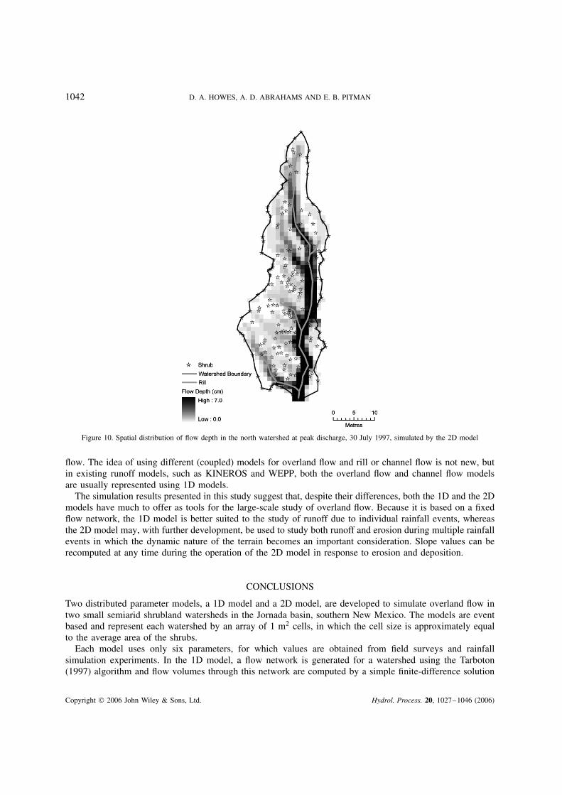
Greyscale images representing the spatial distribution of flow depth at the time of peak discharge for the30 July 1997 storm are shown for the north watershed in Figures 9 and 10 and for the south watershed inFigures 11 and 12. The rills surveyed are also shown in each figure. The images suggest that the modelssimulate the spatial pattern of flow depth in each watershed well, although the differences between the 1Dand 2D representations of the runoff processes are clear. In the 1D model, much of the flow is confined tonarrowly defined flowpaths, especially along the main rill in each watershed, whereas the flow exhibits muchgreater dispersion when represented by the 2D model. Except in a few places in each watershed, the depth offlow in cells along the watershed boundary is small. However, as will be discussed later, some flow acrossthe boundary does occur.

A section of the south watershed is shown in Figures 13 and 14 in order to provide a detailed viewof the 1D and 2D flow patterns. The depth of flow in the main channel is about 3Ð6 cm in the 1Drepresentation, whereas flow is distributed over a wider area in the 2D representation and is, therefore,only about 1Ð85 cm deep at the same point. This 2D representation of the flow in the rills is less real-istic than that for the 1D model, especially in the south watershed. In reality, the rills in this water-shed are well defined and flow is generally confined to a width of less than 1 m. Thus, in the case



Figure 4. Flow network for the south watershed generated by the Tarboton algorithm

0

5000

10000

15000

20000

25000

30000

35000

40000

0 5 10 15 20 25 30

Time (min)

Dis

char

ge (

cm3

s-1)

0

50

100

150

200

250

300

350

400

450

500

550

600

Rai

nfal

l (m

m h

-1)

Observed1D Model2D Model

Figure 5. North watershed observed and simulated hydrographs for the 30 July 1997 storm

of rill cells, the discrete and well-defined flowpaths that are specified by the Tarboton algorithm aremore realistic than the dispersive flow pattern simulated by the 2D model. The 2D model, however, pro-vides a more realistic representation of the flow on the hillslopes between the rills than does the 1Dmodel.



0

5000

10000

15000

20000

25000

30000

35000

0 5 10 15 20 25 30

Time (min)

Dis

char

ge (

cm3

s-1)

0

50

100

150

200

250

300

350

400

450

500

550

600

Rai

nfal

l (m

m h

-1)


Figure 6. South watershed observed and simulated hydrographs for the 30 July 1997 storm

0

2000

4000

6000

8000

10000

12000

14000

16000

18000

20000

0 5 10 15 20 25 30 35 40 45 50

Time (min)

Dis

char

ge (

cm3

s-1)

0

50

100

150

200

250

300

350

400

450

500

550

600

Rai

nfal

l (m

m h

-1)


Figure 7. North watershed observed and simulated hydrographs for the 14 August 1997 storm

Differences between the output from the 1D and 2D models

Flow routing, infiltration, and flow resistance. The primary differences between the performances of the1D and 2D runoff models relate to flow routing, as illustrated by the flow depth images discussed above.In general, the total distance travelled by overland flow in a watershed, which can be referred to as thecumulative flow distance, is smaller when the flow is represented one-dimensionally than when it is representedtwo-dimensionally.



0

1000

2000

3000

4000

5000

6000

7000

8000

0 5 10 15 20 25 30 35 40 45 50

Time (min)

Dis

char

ge (

cm3

s-1)

0

50

100

150

200

250

300

350

400

450

500

550

600

Rai

nfal

l (m

m h

-1)


Figure 8. South watershed observed and simulated hydrographs for the 14 August 1997 storm

The two main consequences of differences in the cumulative flow distance relate to infiltration and flowresistance. An increase in the cumulative flow distance is generally accompanied by an increase in theopportunity for water to infiltrate. The predicted hydrographs suggest that the total volume of infiltrationestimated by the 1D model is consistently less than that estimated by the 2D model. With a lower cumulativeflow distance, the flow encounters lower overall resistance, which causes the runoff hydrograph to be moreflashy than it would be if the flowpaths were longer. Except in the case of the 30 July 1997 south watershedstorm, the peak runoff predicted by the 1D model typically occurs earlier and has a greater magnitude thanthat predicted by the 2D model. The distinction between the 1D and 2D hydrographs is less for the 30 July1997 south watershed storm because of the low values of Ks in this watershed and the significant volume ofrainfall associated with the storm. The watershed became saturated very quickly in both model simulations.At saturation, the amount of infiltration is no longer the dominant factor affecting the model output, anddifferences between the hydrographs are related only to the more minor effect of flow resistance.

Leakage along the watershed boundary. Differences between the 1D and 2D model hydrographs also reflectthe way each model represents leakage along the boundary of the watershed. Although an attempt was madeto find watersheds with well-defined boundaries, the relief in both the north and south watersheds is so smalland the slopes are so gentle that some leakage along the watershed boundary is inevitable. For each simulationrun, the relative amount of water leaving the watershed along the boundary was estimated from a balancecheck. The water balance was computed at the end of each run by subtracting the total volumes of runoff,infiltration, and water left on the watershed surface, from the total volume of rainfall.

In the case of the 30 July 1997 storm (Figures 5 and 6) for the 1D model, 0Ð75% of the total rainfall in thenorth watershed left the watershed at points other than the outflow. For the same storm, however, a 5Ð33%loss across the boundary was simulated by the 2D model. The increased loss simulated by the 2D model andthe increased volume of infiltration simulated by this model account for the differences between the 1D and2D hydrographs for the storm.

By contrast, for the same storm at the south watershed, the 1D model simulates a 3Ð74% loss of wateracross the boundary, whereas the 2D model simulates a loss of only 1Ð62%. The increased runoff simulatedby the 1D model is adequately explained by the lower amount of infiltration simulated by this model.



Figure 9. Spatial distribution of flow depth in the north watershed at peak discharge, 30 July 1997, simulated by the 1D model. The rillsand watershed boundary are defined by the survey data

1D versus 2D models

When comparing the 1D and 2D models developed in this study it is important to bear in mind thefundamental differences between the models. The second-order accurate numerical scheme employed to solvethe kinematic wave equation in the 2D model has a sound mathematical and physical basis. The model isversatile, in that the flow network for a watershed does not have to be specified in advance and the numericalscheme is able to integrate converging flows smoothly, despite the rapidly changing flow conditions typicalof the north and south watersheds.

In contrast to the 2D model, the 1D model is based on a flow structure that is fixed for the duration of arunoff event and employs a somewhat crude application of a first-order accurate numerical scheme to solvethe kinematic wave equation and thus compute the volume of flow through the network. The application ofthe numerical scheme is crude because it assumes (1) that inflows to a cell can be summed and treated as ifthey had originated in one place and (2) that flow from a cell may be simply divided between two downslopecells according to the direction of a single slope value computed for the cell. As a result of these assumptions,flow integration is carried out less smoothly than in the 2D model. With respect to the spatial distribution ofoverland flow, the 1D model performs better than the 2D model where flow is concentrated into well-definedflowpaths (e.g. rills), whereas the 2D model is better suited to simulating dispersed interrill flow on hillslopeswith no rills or channels. This suggests that, in order to model overland flow in the shrubland environmentmore realistically, it may be appropriate to combine a 2D model for interrill flow with a 1D model for rill



Figure 10. Spatial distribution of flow depth in the north watershed at peak discharge, 30 July 1997, simulated by the 2D model

flow. The idea of using different (coupled) models for overland flow and rill or channel flow is not new, butin existing runoff models, such as KINEROS and WEPP, both the overland flow and channel flow modelsare usually represented using 1D models.

The simulation results presented in this study suggest that, despite their differences, both the 1D and the 2Dmodels have much to offer as tools for the large-scale study of overland flow. Because it is based on a fixedflow network, the 1D model is better suited to the study of runoff due to individual rainfall events, whereasthe 2D model may, with further development, be used to study both runoff and erosion during multiple rainfallevents in which the dynamic nature of the terrain becomes an important consideration. Slope values can berecomputed at any time during the operation of the 2D model in response to erosion and deposition.

CONCLUSIONS

Two distributed parameter models, a 1D model and a 2D model, are developed to simulate overland flow intwo small semiarid shrubland watersheds in the Jornada basin, southern New Mexico. The models are eventbased and represent each watershed by an array of 1 m2 cells, in which the cell size is approximately equalto the average area of the shrubs.

Each model uses only six parameters, for which values are obtained from field surveys and rainfallsimulation experiments. In the 1D model, a flow network is generated for a watershed using the Tarboton(1997) algorithm and flow volumes through this network are computed by a simple finite-difference solution



Figure 11. Spatial distribution of flow depth in the south watershed at peak discharge, 30 July 1997, simulated by the 1D model

to the 1D kinematic wave equation. In the 2D model, flow directions and volumes are computed by a second-order predictor–corrector finite-difference solution to the 2D kinematic wave equation, in which flow routingis implicit and may vary in response to flow conditions.

The models are compared in terms of the runoff hydrograph and the spatial distribution of runoff for twostorms. The results show that both models are capable of providing accurate predictions of the runoff fromthe watersheds. However, the 1D model concentrates overland flow more quickly and predicts greater flowvelocities than the 2D model does. As a result, the 1D model tends to overpredict observed peak discharges,whereas the 2D model tends to underpredict observed peak discharges. Despite these differences, the simulationresults suggest that both the 1D and the 2D models have much to offer as tools for the large-scale studyof overland flow. Because it is based on a fixed flow network, the 1D model is better suited to the studyof runoff due to individual rainfall events, whereas the 2D model may, with further development, be usedto study both runoff and erosion during multiple rainfall events in which the dynamic nature of the terrainbecomes an important consideration.

ACKNOWLEDGEMENTS

This research was supported by the National Science Foundation Jornada Basin Long-Term EcologicalResearch (LTER) project (DEB 94-11971) and the National Center for Geographic Information and Analysis(SBR 88-10917), University at Buffalo, The State University of New York. We are grateful to John Andersonand the LTER technicians at New Mexico State University, Las Cruces, for operating and maintaining thehydrometeorological instruments in the two watersheds; to Kris Havstad and staff at the USDA-ARS Jornada



Figure 12. Spatial distribution of flow depth in the south watershed at peak discharge, 30 July 1997, simulated by the 2D model

Figure 13. Detailed view of the spatial distribution of flow depth in the south watershed at peak discharge, 30 July 1997, simulated by the1D model



Figure 14. Detailed view of the spatial distribution of flow depth in the south watershed at peak discharge, 30 July 1997, simulated by the2D model

Experimental Range for building the supercritical flumes and providing the tanker truck; and to Melissa Neave,Scott Rayburg, and Scott McCabe, University at Buffalo, for their assistance with the fieldwork.

REFERENCES

Abrahams AD, Neave M, Schlesinger WH, Wainwright J, Howes DA, Parsons AJ. 2005. Fluxes of water and materials: processes andcontrols. In Structure and Function of a Chihuahuan Desert Ecosystem: The Jornada Basin Long-Term Research Site, Schlesinger WH,Huenneke L, Havstad K (eds). Oxford University Press: Oxford, UK.

Baird AJ. 1997. Overland flow generation and sediment mobilisation by water. In Arid Zone Geomorphology: Process, Form and Changein Drylands , second edition, Thomas DSG (ed.). Wiley: New York; 153–215.

Bathurst JT. 1986. Physically-based distributed modelling of an upland catchment using the Systeme Hydrologique Europeen. Journal ofHydrology 87: 79–102.

Beven K. 1989. Changing ideas in hydrology—the case of physically-based models. Journal of Hydrology 105: 157–172.Chow VT. 1959. Open Channel Hydraulics . McGraw-Hill: London.Davis SF. 1988. Simplified second-order Godunov-type methods. SIAM Journal of Scientific and Statistical Computing 9: 445–473.ESRI. 1998. ArcInfo User Manual . Environmental Systems Research Institute, Inc.: Redlands, CA.Flanagan DC, Nearing MA (eds). 1995. USDA-water erosion prediction project hillslope profile and watershed model documentation . NSERL

Report 10, National Soil Erosion Laboratory, West Lafayette, IN.Freeze RA. 1980. A stochastic-conceptual analysis of rainfall-runoff processes on a hillslope. Water Resources Research 16: 391–408.Gao X, Sorooshian S, Goodrich DC. 1993. Linkage of a GIS to a distributed rainfall-runoff model. In Environmental Modeling with GIS ,

Goodchild MF, Parks BO, Steyaert LT (eds). Oxford University Press: New York; 182–187.Goodrich DG, Woolhiser DA, Keefer TO. 1991. Kinematic routing using finite elements on a triangular irregular network. Water Resources

Research 27: 995–1003.Grayson RB, Moore ID, McMahon TA. 1992a. Physically based hydrologic modeling 1. A terrain-based model for investigative purposes.

Water Resources Research 28: 2639–2658.Grayson RB, Moore ID, McMahon TA. 1992b. Physically based hydrologic modeling 2. Is the concept realistic? Water Resources Research

28: 2659–2666.Howes DA, Abrahams AD. 2003. Modeling runoff and runon in a desert shrubland ecosystem, Jornada basin, New Mexico. Geomorphology

53: 45–73.Martinez-Meza E, Whitford WG. 1996. Stemflow, throughfall and channelization of stemflow by roots in three Chihuahuan desert shrubs.

Journal of Arid Environments 32: 271–287.Moore ID, Grayson RB. 1991. Terrain-based catchment partitioning and runoff prediction using vector elevation data. Water Resources

Research 27: 1177–1191.Navar J, Bryan R. 1990. Interception loss and rainfall redistribution by three semi-arid growing shrubs in northeastern Mexico. Journal of

Hydrology 115: 51–63.



Nielsen DR, Biggar JW, Erh KT. 1973. Spatial variability of field measured soil-water properties. Hilgardia 42: 215–260.Noy-Meir I. 1985. Desert ecosystem structure and function. In Hot Deserts and Arid Shrublands , Evanari M, Noy-Meir I, Goodall DW

(eds). Elsevier: Amsterdam; 93–103.Onstad CA, Brakensiek DL. 1968. Watershed simulation by the stream path analogy. Water Resources Research 4: 965–971.Parsons AJ, Wainwright J, Abrahams AD, Simanton JR. 1997. Distributed dynamic modelling of interrill overland flow. Hydrological

Processes 11: 1838–1859.Ponce VM. 1991. The kinematic wave controversy. Journal of Hydraulic Engineering 117: 511–525.Refsgaard JC. 1997. Parameterisation, calibration and validation of distributed hydrological models. Journal of Hydrology 198: 69–97.Refsgaard JC, Storm B. 1996. Construction, calibration and validation of hydrological models. In Distributed Hydrological Modelling ,

Abbott MB, Refsgaard JC (eds). Kluwer: Dordrecht, The Netherlands; 41–54.Reynolds JF, Virginia RA, Schlesinger WH. 1997. Defining functional types for models of desertification. In Plant Functional Types:

Their Relevance to Ecosystem Properties and Global Change, Smith TM, Shugart HH, Woodward FI (eds). Cambridge University Press:Cambridge, UK; 194–214.

Saint Venant B de. 1871. Theory of unsteady water flow, with application to river floods and to propagation of tides in river channels.French Academy of Science 73.

Schlesinger WH, Jones CS. 1984. The comparative importance of overland runoff and mean annual rainfall to shrub communities of theMojave Desert. Botanical Gazette 145: 116–124.

Schlesinger WH, Abrahams AD, Parsons AJ, Wainwright J. 1999. Nutrient losses in runoff from grassland and shrubland habitats in southernNew Mexico: 1. Rainfall simulation experiments. Biogeochemistry 45: 21–34.

Scoging HM, Parsons AJ, Abrahams AD. 1992. Application of a dynamic overland-flow hydraulic model to a semi-arid hillslope, WalnutGulch, Arizona. In Overland Flow Hydraulics and Erosion Mechanics , Parsons AJ, Abrahams AD (eds). UCL Press: London, UK;105–145.

Sherman B, Singh VP. 1976. A distributed converging overland flow model: 1. Mathematical solutions. Water Resources Research 12:889–896.

Singh VP. 1996. Kinematic Wave Modeling in Water Resources: Surface-Water Hydrology . John Wiley: New York.Smith RE, Parlange J-Y. 1978. A parameter-efficient hydrologic infiltration model. Water Resources Research 14: 533–538.Smith RE, Goodrich DG, Woolhiser DA, Unkrich CL. 1995. KINEROS—KINematic runoff and EROSion model. In Computer Models of

Watershed Hydrology , Singh VP (ed.). Water Resources Publications: Fort Collins, CO; 697–732.Springer EP, Cundy TW. 1987. Field scale evaluation of infiltration parameters from soil texture for hydrologic analysis. Water Resources

Research 23: 325–341.Tarboton DG. 1997. A new method for the determination of flow directions and upslope areas in grid digital elevation models. Water

Resources Research 33: 309–319.Vertessy RA, Hatton TJ, O’Shaughnessy PJ, Jayasuriya MDA. 1993. Predicting water yield from a mountain ash forest catchment using a

terrain analysis based catchment model. Journal of Hydrology 150: 665–700.Woolhiser DA, Smith RE, Goodrich DC. 1990. KINEROS: A Kinematic Runoff and Erosion Model: Documentation and User Manual . US

Department of Agriculture, Agricultural Research Service Report No. 77, Fort Collins, CO.Zhang W, Cundy TW. 1989. Modeling of two-dimensional overland flow. Water Resources Research 25: 2019–2035.


one‐ and two‐dimensional modelling of overland flow in

Documents