optimal campaigning in presidential elections: the probability of
TRANSCRIPT

Seminar Paper No. 706
OPTIMAL CAMPAIGNING IN PRESIDENTIAL
ELECTIONS: THE PROBABILITY OF BEING
FLORIDA
by
David Strömberg
INSTITUTE FOR INTERNATIONAL ECONOMIC STUDIES Stockholm University

Seminar Paper No. 706
OPTIMAL CAMPAIGNING IN PRESIDENTIAL ELECTIONS:
THE PROBABILITY OF BEING FLORIDA
by David Strömberg
Papers in the seminar series are published on the internet in Adobe Acrobat (PDF) format. Download from http://www.iies.su.se/ Seminar Papers are preliminary material circulated to stimulate discussion and critical comment. March 2002 Institute for International Economic Studies
S-106 91 Stockholm Sweden
Optimal Campaigning in Presidential Elections:The Probability of Being Florida
David Strömberg∗
IIES, Stockholm University
April 23, 2002
Abstract
This paper delivers a precise recommendation for how presidential candi-dates should allocate their resources to maximize the probability of gaininga majority in the Electoral College. A two-candidate, probabilistic-votingmodel reveals that more resources should be devoted to states which arelikely to be decisive in the electoral college and, at the same time, have veryclose state elections. The optimal strategies are empirically estimated usingstate-level opinion-polls available in September of the election year. Themodel’s recommended campaign strategies closely resemble those used inactual campaigns. The paper also analyses how the allocation of resourceswould change under the alternative electoral rule of a direct national votefor president.
∗[email protected], IIES, Stockholm university, S-106 91 Stockholm.I thank Steven Brams, Steve Coate, Antonio Merlo, Torsten Persson, Gerard Roland, TomRomer, Howard Rosenthal, Jim Snyder, Jörgen Weibull, and seminar participants at UC Berke-ley, Cornell university, the CEPR/IMOP Conference in Hydra, New York university, Stan-ford university, University of Pennsylvania, Princeton university, and the Wallis Conferencein Rochester. Previous versions have been circulated under the titles: ”The Lindbeck-Weibullmodel in the Federal US Structure”, and, ”The Electoral College and Presidential ResourceAllocation”s.JEL-classification, D72, C50, C72, H50, M37.Keywords: elections, political campaigns, public expenditures

1. Introduction
This paper explores how the Electoral College shapes incentives for presidentialcandidates to allocate resources across states. It does so by developing a prob-abilistic voting model of electoral competition under the US Electoral Collegesystem.1 The model delivers a precise recommendation for how presidential can-didates, trying to maximize the probability of gaining a majority in the ElectoralCollege, should allocate their resources. This recommendation is fully charac-terized, both theoretically and empirically. The recommendations of the modelare then compared to the actual presidential campaign visits across states duringthe 1988-2000 presidential elections, and to presidential campaign advertisementsacross media markets in the 2000 election. The actual allocation of these re-sources closely resembles the equilibrium allocation in the model. The paperfinally analyses how the allocation of advertisements across media markets wouldchange under an institutional reform, namely the transition to a direct nationalvote for president. The principles guiding the allocation are quite different underthe two systems, and the incentives to favor certain markets are much strongerunder the Electoral College than under the Direct Vote, causing a more unequaldistribution of resources.In an early game-theoretic analysis of the effects of the Electoral College sys-
tem, Brams and Davis (1974) find that presidential candidates should allocateresources disproportionately in favor of large states. They use a model wherevotes are cast with equal probability for each candidate, and where the candidatesmaximize their expected number of electoral votes. Their result is disputed byColantoni, Levesque and Ordeshook (1975) who instead argue that a proportionalrule, modified to take into account the closeness of the state election, predictsactual campaign allocations better. In his model of two-party competition for leg-islative seats, Snyder (1989) allows parties to have advantages in certain districtsand finds that equilibrium campaign allocations are higher in close districts. Fur-ther, if the goal of the parties is to maximize the probability of winning a majorityof seats, then allocations are also higher in districts which are more likely to bepivotal. Finally, more resources will be spent in safe districts of the advantagedparty than in the safe districts of the other party.
1In this system, a direct vote election is held in each state and the winner of the vote issupposed to get all of that states electoral votes. Then all the electoral votes are counted, andthe candidate who receives most votes wins the election. (The fact that Maine and Nebraskaorganize their presidential elections by congressional district is disregarded in this paper.)
2

Inspired by these results, Nagler and Leighley (1992) empirically investigatestate-by-state campaign expenditures on non-network advertising in 1972 and findthese to be higher in states with closer elections andmore electoral votes. A relatedempirical literature studies the political influence on allocations of federal fundsacross states. Wright (1974) finds that federal spending between 1933 and 1940was higher in states with higher “political productivity”, a measure dependingon the electoral votes per capita, the variability in the vote share of the incum-bent government in past elections, and the predicted closeness of the presidentialelections. For a more recent contribution to this literature, see Wallis (1996).A separate theoretical literature has analyzed the policy effects of plurality
versus proportional representation election systems. For example, Persson andTabellini (1999), and Lizzeri and Persico (2001), find that under plurality rulegovernments tend to overprovide redistributive spending because its benefits canbe more easily targeted to voters than public goods.The main contribution of this paper is that it develops a model that is em-
pirically estimable and allows for explicit solutions. It therefore ties together, ina precise way, theoretical insights similar to those of Brams and Davis (1974),Snyder (1989), Persson and Tabellini (1999), and Lizzeri and Persico (2001), withempirical results on actual campaigns or distribution of federal funds, similar tothose of Nagler and Leighley (1992), and Wright (1974). The model also extendsthe theory of the Electoral College. It allows for differences in preferences acrossstates, it allows for vote outcome across states to be correlated, and it allows forexplicit solutions. This yields new theoretical insights. The model also revealsa link between all of the above literature and the literature concerning ”votingpower”, that is, the probability that a vote is decisive in an election (Banzaf(1968), Chamberlain and Rothschild (1988), Gelman and Katz (2001), Gelman,King and Boscardin (1998)), and Merrill (1978)). The equilibrium allocation ofresources is found to be proportional to the ”voting power” under the ElectoralCollege system, but not under Direct Vote.This is the first in a series of three papers. Here, I develop a theory of polit-
ical redistribution under the Electoral College and test it on instruments wherethe presidential candidates have clear control and clear objectives. In Strömberg(2002a), I study an area where presidential control is less clear and objectives aremore multi-faceted, but where the welfare effects are larger. That paper findssimilar patterns of Electoral College effects on the allocation of federal civilianemployment across states 1948-1996. In Strömberg (2002b), I study voter partic-ipation. That paper adds political competition under the Electoral College to the
3

model of Shachar and Nalebuff (1999). As these applications, and the discussionof the change to a Direct Vote system, show, the estimable probabilistic-votingmodel developed in this paper is very general and can be applied to a wide varietyof electoral settings and questions.Section 2 develops the theoretical model. It also estimates the probability
distribution for election outcomes suggested by the model empirically, and usesthese estimates to interpret the equilibrium. Section 3 confronts the models pre-dictions with actual campaign efforts. Section 4 addresses the allocational effectsof a change to a Direct Vote system. Finally, Section 5 discusses the results andconcludes.
2. Model
Two presidential candidates, indexed by superscript R and D, try to maximizetheir expected probability of winning the election by selecting the number of days,ds, to campaign in each state s, subject to the constraint
SXs=1
dJs ≤ I,
J = R,D. In each state s, there is an election. The candidate who receives amajority of the votes in that state gets all the es electoral votes of that state.After elections have been held in all states, the electoral votes are counted, andthe candidate who gets more than half those votes wins the election.There is a continuum of voters, each indexed by subscript i, a mass vs of which
live in state s. Campaigning in a state increases the popularity of the campaigningcandidate among voters in that state, as captured by the increasing and concavefunction u
¡dJs¢.2 The voters also care about some fixed characteristics of the
candidates, captured by parameters Ri, ηs, and η. The parameter Ri representsan individual-specific ideological preference in favor of candidate R, and ηs and ηrepresent the general popularity of candidateR. The voters may vote for candidateR or candidate D, and voter i in state s will vote for D if
∆us = u¡dDs¢− u ¡dRs ¢ ≥ Ri + ηs + η. (2.1)
2This paper does not address the question of why campaigning matters. This is an interestingquestion in its own right, with many similarities to the question of why advertisements affectconsumer choice.
4

At the time when the campaign strategies are chosen, there is uncertaintyabout the popularity of the candidates on election day. This uncertainty is cap-tured by the random variables ηs and η. The candidates know that the S statelevel popularity parameters, ηs, and the national popularity parameter, η, areindependently drawn from cumulative distribution functions Gs = N(0,σ2s), andH = N (0,σ2) respectively, but they do not know the realized values.The distribution of voters’ ideological preferences, Ri, within each state is
Fs = N¡µs,σ
2fs
¢, a normal distribution with mean µs and variance σ2fs. The
means of the states’ ideological distributions may shift over time, but the varianceis assumed to remain constant. The share of votes that candidate D receives instate s is
Fs(∆us − ηs − η).
This candidate wins the state if
Fs(∆us − ηs − η) ≥ 12,
or, equivalently, ifηs ≤ ∆us − µs − η.
The probability of this event, conditional on the aggregate popularity η, and thecampaign visits, dDs , and d
Rs , is
Gs (∆us − µs − η) . (2.2)
Let es be the number of votes of state s in the Electoral College. Define sto-chastic variables, Ds, indicating whether D wins state s
Ds = 1, with probability Gs (·) ,Ds = 0, with probability 1−Gs (·) .
The probability that D wins the election is then
PD¡dD, dR, η
¢= Pr
"Xs
Dses >1
2
Xs
es
#. (2.3)
However, it is difficult to find strategies which maximizes the expectation of theabove probability of winning. The reason is that it is a sum of the probabilitiesof all possible combinations of state election outcomes which would result in D
5

winning. The number of such combinations is of the order of 250, for each of theinfinitely many realizations of η.A way to cut this Gordian knot, and to get a simple analytical solution to
this problem, is to assume that the candidates are considering their approximateprobabilities of winning. Since the ηs are independent, so are the Ds. Thereforeby the Central Limit Theorem of Liapounov,P
sDses − µσE
whereµ = µ
¡dD, dR, η
¢=Xs
esGs (∆us − µs − η) , (2.4)
andσ2E = σ2E
¡dD, dR, η
¢=Xs
e2sGs (·) (1−Gs (·)) , (2.5)
is asymptotically distributed as a standard normal. The mean, µ, is the expectednumber of electoral votes. That is, the sum of the electoral votes of each state,multiplied by the probability of winning that state. The variance, σ2E, is thesum of the variances of the state outcomes, which is the e2s multiplied by theusual expression for the variance of a Bernoulli variable. Using the asymptoticdistribution, the approximate probability of D winning the election is
ePD ¡dD, dR, η¢ = 1− Φ
µ 12
Ps es − µσE
¶.
The error made from using the approximate probability of winning is discussed inSection 2.2, and Appendix 6.8.Candidate D maximizes the approximate probability of winning the election
maxdDPD
¡dD, dR
¢= max
dD
Z ePD ¡dD, dR, η¢h (η) dηsubject to the constraint X
dDs = I.
Candidate R also maximizes his approximate probability of winning. This gamehas a unique, interior, pure-strategy equilibrium characterized by the proposition
6

below.3 In Section 2.1, the functions u (ds) are chosen to ensure interior equilibria.Non-interior equilibria are characterized in Appendix 6.2.
Proposition 1. The unique pair of strategies for the candidates¡dD, dR
¢that
constitute a NE in the game of maximizing the expected probability of winningthe election must satisfy dD = dR = d∗, and for all s and for some λ > 0
Qsu0 (d∗s) = λ, (2.6)
where
Qs = −Z
∂
∂∆usΦ
µ 12
Ps es − µσE
¶h (η) dη.
Proof: See Appendix 6.1.Proposition 1 says that presidential candidates who are trying to maximize
their probability of winning the election should spend more time in states withhigh values of Qs. This follows since u0 (d∗s) is decreasing in d
∗s. The following
pages will be devoted to exploring what Qs represents and how to measure it.First, note that Qs consists of two additively separable parts:
Qs = −Z µ
∂Φ (·)∂µ
∂µ
∂∆us+
∂Φ (·)∂σE
∂σE∂∆us
¶h (η) dη = Qsµ +Qsσ. (2.7)
One arises because the candidates have an incentive to influence the expectednumber of electoral votes won by D, that is the mean of the normal distribution.The other arises because the candidates have an incentive to influence the variancein the number of electoral votes. The empirical discussion will be organized todiscuss each term separately.A qualified guess is that Qs is approximately the joint ”likelihood” that a
state is actually decisive in the Electoral College and, at the same time, has atied election. I will call states who are ex post decisive in the Electoral Collegeand have tied elections decisive swing states. In the 2000 election, Florida was a
3Note that the candidates have diametrically opposed preferences, in other words, this is azerosum game. This implies that the equilibrium strategies are as if each candidate tried tominimize the maximum probability that the other candidate could get by allocating resourcesacross states. The same equilibrium would result in a game where one candidate moved first, andthen the other, taking the first candidate’s strategy as given. The first candidate would minimizethe maximum that the second player could attain. And the second player would maximize thisprobability of winning given the first candidate’s strategy.
7

decisive swing state. In contrast, neither New Mexico nor Wyoming were decisiveswing states. While New Mexico was a swing state with a very close electionoutcome, it was not decisive in the Electoral College since Bush would have wonwith or without the votes of New Mexico. While Wyoming was decisive in theElectoral College, since Gore would have won the election, had he won Wyoming,it was not a swing state.The above guess is based on the fact that the probability of being a decisive
swing state replaces Qs in the equilibrium condition of the model without theCentral Limit approximation.4 Further, Appendix 6.3 shows that Qsµ and Qsσapproximately equals the first and second-order parts of a second-order Taylor-expansion of the approximate probability of being a decisive swing state. In theempirical section, the values of the analytical expression for Qs will be comparedwith the probability that a state is decisive in the Electoral College and, at thesame time has a state margin of victory of less than two percent. To measure thisprobability, I now estimates the probability distribution for election outcomes.
2.1. Estimation
In equilibrium, both candidates choose the same allocation, so that ∆us = 0 inall states. The Democratic vote-share in state s at time t equals
yst = Fst (−ηst − ηt) = Φ
µ−µst − ηst − ηtσfs
¶,
where Φ (·) is the standard normal distribution, or equivalently,
Φ−1(yst) = γst = −1
σfs(µst + ηst + ηt) . (2.8)
For now, assume that all states have the same variance of preferences, σ2fs = 1,and the same variance in state-specific shocks, σ2s.
5 Further assume that the meanof the preference distribution, µst, depends on a set of variables Xst , so that theestimated equation is
γst = − (βXst + ηst + ηt) . (2.9)4Unfortunately, I can not compute the analytical solution of that model.5These assumptions will be removed in Section 4. However, the estimates become imprecise
if separate values of µst, σfs, and σs are estimated for each state using only 14 observations perstate. Therefore, the more restrictive specification will be used for most of the paper.
8

The parameters β,σs and σ are estimated using a standard maximum-likelihoodestimation of the above random-effects model.6
The variables in Xst are basically those used in Campbell (1992). The nationalvariables are: the Democratic vote share of the two-party vote share in trial-heat polls from mid September (all vote-share variables x are transformed byΦ−1(x)); second quarter economic growth; incumbency; and incumbent presidentrunning for re-election. The state variables for 1948-1984 are: lagged and twicelagged difference from the national mean of the Democratic two-party vote share;the first quarter state economic growth; the average ADA-scores of each state’sCongress members the year before the election; the Democratic vote-share of thetwo-party vote in the midterm state legislative election; the home state of thepresident; the home state of the vice president; and dummy variables describedin Campbell (1992). After 1984, state-level opinion-polls were available. For thisperiod, the state-level variables are: lagged difference from the national meanof the Democratic vote share of the two-party vote share; the average ADA-scores of each state’s Congress members the year before the election; and thedifference between the state and national polls. The other state-level variableswere insignificant when state polls were included. The coefficients β and thevariance of the state level popularity shocks, σ2s, are allowed to differ for whenopinion polls were available and when they were not. The equation yields forecastsby mid September of the election year. The data-set contains state elections forthe 50 states 1948-2000, except Hawaii and Alaska which began voting in the1960 election. During this period there were a total of 694 state-level presidentialelection results. Of this total, 13 state elections were excluded, leaving a total of681 observations. Four elections in Alaska and Hawaii were excluded because therewere no lagged vote returns. Nine elections are omitted because of idiosyncrasiesin Presidential voting in Alabama in 1948, and 1964, and in Mississippi in 1960;see Campbell (1992).
6The model was also extended to include regional swings. In this specification, the electionresult in one state equals
yst = Fst (ηst + ηrt + ηt) ,
where ηrt denotes independent popularity shocks in the Northeast, Midewest, West, and South.The estimated variances of the state and national level shocks are similar to those estimatedwithout allowing for regional shocks, σs,post1984 = 0.084, and σ = 0.038, see Appendix 6.4. Thestandard deviation of the regional shock is σr = 0.054 before state level forecasts where availablein 1988. However, after 1988, the standard deviation of the regional shocks is zero. Taking intoaccount the information of september state-level opinon polls, there are no significant regionalswings. Therefore, the simpler specification without regional swings is used below.
9

The estimation results are shown in Table 1. The standard deviation of thestate level shocks after 1984 , σs, equals 0.077, or about 3% in vote shares. Thisis more than twice as large as that of the national shocks, σ = 0.033. Theaverage error in state election vote forecasts is 3.0 percent and the wrong winneris predicted in 14 percent of the state elections. This is comparable to the beststate-level election-forecast models (Campbell, 1992; Gelman and King, 1993;Holbrook and DeSart, 1999; Rosenstone, 1983).
2.2. Characterization of equilibrium
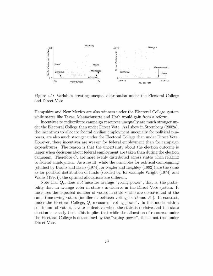
Next, I test whether Qs approximately equals the probability of being a decisiveswing state. To this end, one million electoral vote outcomes were simulated foreach election 1988-2000 by using the estimated state-means, and drawing state andnational popularity-shocks from their estimated distributions. Then, the share ofelections where a state was decisive in the Electoral College and at the sametime had a state election outcome between 49 and 51 percent was recorded. Thisprovides an estimate which should be roughly equal to Qs. Figure 2.1, containsthese shares on the y-axis and values computed from the analytic expression ofQs, on the x-axis. Large states are trivially more likely to be decisive. To checkthat the correlation between Qs and the simulated values is not just a matter ofsize, the graph on the right contains the same series divided by the state’s numberof electoral votes. The simple correlation in the diagram to the right is 0.997. Sothe two variables are interchangeable, for practical purposes. The 0.003 differencecould result on the Qs-side from using the approximate probability of winning theelection, and on the simulation-side from using a finite number of simulations andrecording state election results between 49 and 51 percent, whereas theoreticallyit should be exactly 50 percent.
To illustrate the discussion of how Qs varies across states, I will use the year2000 election, see Figure 2.2. Based on polls available in mid September, 2000,Florida, Michigan, Pennsylvania, California, and Ohio were the states most likelyto be decisive in the Electoral College and at the same time have a state elec-tion margin of less than 2 percent. This happened in 2.2 to 3.4 percent of thesimulations.
The analytic expression for Qs explains exactly why some states are morelikely to be decisive swing states. First, Qs is roughly proportional to the num-ber of electoral votes. The reason is that the change in the expected number of
10

Pivo
tal a
nd c
lose
per
ele
ctor
al v
ote
Qs per electoral vote0 .0020
.002
Sim
ulat
ed s
hare
piv
otal
and
clo
se e
lect
ions
Qs0 .0550
.047
Figure 2.1: Qs and simulated probability of being a decisive swing state
electoral votes in response to an extra candidate visit to a state is proportionalto the number of electoral votes of that state. Therefore, so is Qsµ. The changein the variance, and therefore Qsσ, is proportional to the state’s electoral votessquared. As Qsσ is generally considerably smaller than Qsµ, Qs is roughly propor-tional to the number of electoral votes. This implies that candidates should, onaverage, spend more time in large states. However, for states of equal size thereis considerable variation.7
This can be seen in Figure (2.3). The x-axis shows the forecasted Democraticvote share. The circular dots show the share of the simulated elections where astate was decisive in the Electoral College and at the same time had a state-electionoutcome between 49 and 51 percent, per electoral vote. The solid normal-formline shows Qsµ/es which arises because the candidates try to affect the expectednumber of electoral votes, see equation (2.7). This part of Qs/es accounts formost of the variation in the simulated values. It explains why states like NewYork and Texas are never in a million simulated elections decisive in the ElectoralCollege and at the same time have close state elections, while in Florida, Michigan,Pennsylvania, and Ohio this happens quite frequently. The solid line is in fact anormal distribution, multiplied by a constant. It is characterized by three features:its amplitude, its mean, and its variance.
7This can be contrasted to the finding that voters in larger states should receive more thanproportional attention (Banzaf 1967, Brams and Davis 1974, Gelman and Katz 2001). Theirresults depend on all voters being equally likely to vote for one candidate or the other. Myresults differ since voters are not equally likely to vote for each candidate, and since there areaggregate popularity shocks, see Chamberlain and Rothschild (1981).
11

0 0,5 1 1,5 2 2,5 3 3,5
Hawaii
New York
Vermont
South Carolina
Alaska
Alabama
South Dakota
North Dakota
Montana
Maine
Wyoming
Maryland
Indiana
West Virginia
Virginia
Mississippi
Connecticut
Delaware
New Jersey
Minnesota
Nevada
Arizona
New Hampshire
Georgia
New Mexico
North Carolina
Colorado
Arkansas
Kentucky
Iowa
Illinois
Oregon
Louisiana
Washington
Wisconsin
Tennessee
Missouri
Ohio
California
Pennsylvania
Michigan
Florida
percent
(Utah, Texas, Rhode Island, Oklahoma, Texas, Nebraska, Massachusetts, Kansas, Idaho) = 0
Figure 2.2: Joint probability of being pivotal and having a state margin of victoryless than two percent, based on September 2000 opinion polls.
12

Simulated values, pivotal and close /es
Forecasted democratic vote share
30 40 50 60 700
.0005
.001
.0015Michigan (18)
PennsylvaniaOhio
California
New YorkTexasWyoming
µ∗s
Qsµ /es
Figure 2.3: Probability of being a decisive swing state per electoral vote.
The amplitude of all Qsµ is trivially higher when the national election is ex-pected to be close. Define eηt to be the national popularity-swing which would giveequal expected Electoral Vote shares, µ (eη) = 1
2
Ps es. Then Qsµ is larger when eηt
is close to zero, that is, when the national election is expected to be close.8 Thevalue of eηt affects all states in a single election in the same way. It explains whythe average Qsµ varies between elections.Notice that the mean is located slightly above 50%. Since we have an analytic
expression for Qs, it is possible to say exactly why this is the case. The meanequals
µ∗st = −σ2
σ2 + (σE/a)2eηt, (2.10)
whereat =
Xs
esgs (−µst − eηt) .The mean always lies between a pro-Republican state bias of µst = 0, whichcorresponds to a 50% forecasted Democratic vote share, and µst = −eηt, whichapproximately corresponds to the forecasted national Democratic vote share. (Ifthe Democrats are ahead by 60-40 nationally, then a pro-Republican swing eηt,
8See equation (6.4) in the Appendix.
13

corresponding to about 10%, is needed to draw the election. Therefore µst = −eηtcorresponds to 10% pro-democrat bias in a state, that is, a vote share of 60-40.)The intuition is the following. Suppose that the Democrats are ahead 60-40
in the national polls, 50-50 in Texas, and 60-40 in Pennsylvania. A candidatevisit may only affect a state outcome in swing states, where the state electionis close. Candidate visits are therefore more likely to influence the outcome inforecasted swing states like Texas, than in states like Pennsylvania. For thisreason, candidates should target states like Texas.However, the candidates must condition their visit strategies on what must
be true for a state to be a swing state on election day. If Texas is still a swingstate on election day, then the Democrats are probably winning by a landslide andTexas will not be decisive. If Pennsylvania is a swing state, then it is likely thatthe election at the national level close and Pennsylvania decisive. For this reasoncandidates should target states like Pennsylvania. The logic resembles that of thewinners curse in auction theory. There the size of the bid only matter when thebid is highest, and the bidders must condition their bid on the circumstance inwhich it matters. Here the visit only matters if the state is a swing state, and thecandidates must condition their visits on this circumstance.The model shows how to strike a balance between high average influence
(Texas) and influence when it matters (Pennsylvania). Basically, the less cor-related the state election outcomes are, the more time should be spent in 50-50states like Texas. This is evident from equation (2.10). The smaller the variance ofthe national popularity-swings, σ2, the more important it is to target states withexpected outcomes close to 50-50. In the extreme case where this variance equalszero, then µ∗s = 0 and most time should be spent in states like Texas. The reasonis that without national swings, the state outcomes are not correlated, and Texasbeing a swing state on election day carries no information about the outcomes inthe other states. (The winner’s curse does not arise in auctions with independentprivate values.) In the extreme case that σ approaches infinity, µ∗s approaches −eη.Therefore most time should be spent in states like Pennsylvania with a 60-40 ex-pected outcome. In my estimates maximum attention should typically be given tostates in the middle, 55-45 in this example. In September of 2000, Gore was aheadby 1.3 percentage points. The maximum Qsµ/es was obtained for states wherethe expected outcome was a Democratic vote share of 50.8 percent, as illustratedin Figure 2.3.People who are familiar with the market CAPMmodel may prefer the following
analogy. Assets trivially attract more investment if they yield higher returns on
14

average (like Texas), but also if they yield higher return in recessions when returnsare more valuable (like Pennsylvania). The larger the aggregate shocks (nationalpopularity-swings), causing deep recessions and high booms, the more importantit is for assets to yield high return in recessions.Although the normal-shaped curve in Figure 2.3 explains most of the variation
in Qs/es, there are some noteworthy discrepancies. First, Wyoming and two otherstates to the left of the center are noticeably above the normal-shaped curve. Thereason is that I could not find state-level opinion poll data for these states, andthe forecasts for these states are more uncertain. These states actually lie ona normal-shaped curve with a higher variance than that drawn in Figure 2.3.9
These observations illustrate one effect of improved forecasting on the allocationof resources. Better state-level forecasts lead to a more unequal allocation ofcampaign resources as the variance of the normal-shaped distribution of Figure 2.3decreases. States with forecasted vote shares close to the center of that distributionwould gain while states far from the center would loose. Better national-levelforecasts has a similar effect.In Figure 2.3, note also that around its peak, the normal-shaped curve is far
from the simulated probabilities of being a decisive swing state per electoral vote.States to the right of µ∗s, like Michigan and Pennsylvania, generally lie abovethe curve, while states on the left, like Ohio, generally lie below. The differencebetween the simulated values and Qsµ/es arises because the candidates also haveincentives to influence the variance of the electoral vote distribution, even if thismeans decreasing the expected number of electoral votes, see Qsσ in equation(2.7).To get the intuition of why this is rational, consider the following example
from the world of ice-hockey. One team is trailing by one goal and there is onlyone minute left of the game. To increase the probability of scoring an equalizer,the trailing team pulls out the goalie and puts in an extra offensive player. Mostfrequently, the result is that the leading team scores. But the trailing team doesnot care about this, since they are loosing the game anyway. They only care aboutincreasing the probability that they score an equalizing goal, which is higher with
9The variance of the normal-form distribution,
eσ2 = σ2s +1³
1σ2 +
1(σE/a)
2
´ ,depends on the variance in the state, and national, level popularity shocks.
15

an extra offensive player. Therefore, it is better to increase the variance in goals,even though this decreases net expected goals.Similarly, presidential candidates who are behind should try to increase vari-
ance in electoral votes. This is done by spending more time in large states wherethis candidate is behind (putting in an extra offensive player). This is compen-sated by fewer visits to states where this candidate is ahead (pulling the goalie).Candidates who are ahead should try to decrease variance in electoral votes, thussecuring their lead. This is done by spending more time in large states wherethis candidate is ahead, and reducing the number of visits where this candidate isbehind. This leads both candidates to spend more time in large states where theexpected winner is leading. This resounds the result by Snyder (1989) that partieswill spend more in safe districts of the advantaged party than in safe districts ofdisadvantaged party.To formally see why a trailing candidate increases the variance by spending
more time in states with many electoral votes where he is behind, consider equa-tion (2.5) showing the variance, conditional on a national shock. The variance inthe number of electoral votes from a state is proportional to these votes squared.Therefore, the effect on the total variance is larger in large states. Further, thevariance in a state outcome is higher the closer the expected result is to a tie. Byvisiting a state where the leading candidate is ahead, the trailing candidate movesthe expected result closer to a tie, and increases the variance in election outcome.Similarly, decreasing the number of visits to a state where the lagging candidateis leading increases the varianceFigure 2.4 illustrates this effect in the year 2000 election. It plots the values
of the analytical expression for Qsσ/es. The lagging candidate (Bush) should putin extra offensive visits in states like Michigan and Pennsylvania, at the cost ofweakening the defense of states like Ohio. The leading candidate (Gore) should in-crease his defense of states like Michigan and Pennsylvania, at the cost of offensivevisits to Ohio.
3. Relation between Qs and actual campaigns
This section will compare the equilibrium campaign strategies to actual campaignstrategies. The first sub-section will investigate presidential candidate visits tostates in the 2000 election, and also more loosely discuss visits during the 1988-1996 elections. The second sub-section will study the allocation of campaignadvertisements across media markets in the 2000 campaign. Finally, the last sub-
16

30 40 50 60 70-.0001
0
.0001
.0002
Michigan Pennsylvania
Ohio
Varia
nce
effe
ct, Q
sσ/v
s
Forecasted democratic vote shares
Figure 2.4: Incentive to influence variance
section estimates the impact of the actual campaigns on the election results.
3.1. Campaign visits
If one assumes log utility, then the optimal allocation, based on equation (2.6) is,
d∗sPd∗s=
QsPQs, (3.1)
and the number of days spent in each state should be proportional to Qs.The Bush and Gore campaigns were very similar to the equilibrium campaign
based on September opinion polls. The actual number of year 2000 campaignvisits, after the party conventions, and Qs, are shown in Figure 3.1.10 Campaignvisits by vice presidential candidates are coded as 0.5 visits. The model and thecandidates’ actual campaigns agree on 8 of the 10 states which should receivemost attention. Notable differences between theory and practice are found inIowa, Illinois and Maine, which received more campaign visits than predicted, andColorado, which received less. Perhaps extra attention was devoted to Maine since10I am grateful to Daron Shaw for providing me with the campaign data.
17

its (and Nebraska’s) electoral votes are split according to district vote outcomes.Other differences could be because the campaigns had access to information oflater date than mid September, and because aspects not dealt with in this papermatter for the allocation. The raw correlation between campaign visits and Qs is0.91. For Republican visits the correlation is 0.90 and for Democratic visits, 0.88.A tougher comparison is that of campaign visits per electoral vote, ds/es, withQs/es. The correlation between ds/es and Qs/es was 0.81 in 2000.Next, I look at the 1996, 1992, and 1988 campaigns. For these campaigns,
only presidential visits are available. The correlation between visits and Qs duringthose years are: 0.85, 0.64, and 0.76 respectively. But this is mainly a result ofpresidential candidates spending more time in large states. For the 1996, 1992,and 1998 elections, the correlation between ds/es and Qs/es was 0.12, 0.58, and0.25 respectively. An explanation for the poor fit in 1996 and 1988 may be thatthese elections were, ex ante, very uneven. The expected Democratic vote sharesin September of 1996, 1992, and 1988 were 56, 50, and 46 percent. In uneven races,perhaps the candidates have other concerns than maximizing the probability ofwinning the election.A possible explanation for the difference between the actual and optimal cam-
paigns is that presidential candidate visits target media markets instead of states.In Appendix 6.6, this situation is modelled. The main new feature is that thereare spillovers across states as media markets cross state boundaries. This increasesthe number of visits seen in New York and Massachusetts. The presidential can-didates choose to visits the media markets in New York and Boston because theycross into states which are important for re-election concerns. However, this doesnot explain why Iowa, Illinois and Maine received more visits, or why Coloradoreceived less than expected. Instead, as the candidates did not visit New Yorkand Massachusetts, this decreases the correlation between the actual and optimalvisits.A complication is that candidates should consider in what media markets
their visit will be reported, rather than what markets they visit. A presidentialcandidate visit to L.A. may be covered also in surrounding Californian mediamarkets. A more direct way to study targeting of media markets is to examine inwhich media markets the campaigns choose to air their advertisements.
18

0 2 4 6 8 10 12
Hawaii
New York
Vermont
South Carolina
Alaska
Alabama
South Dakota
North Dakota
Montana
Maine
Wyoming
Maryland
Indiana
West Virginia
Virginia
Mississippi
Connecticut
Delaware
New Jersey
Minnesota
Nevada
Arizona
New Hampshire
Georgia
New Mexico
North Carolina
Colorado
Arkansas
Kentucky
Iowa
Illinois
Oregon
Louisiana
Washington
Wisconsin
Tennessee
Missouri
Ohio
California
Pennsylvania
Michigan
Florida
percent
∑ s
s
(Utah, Texas, Rhode Island, Oklahoma, Texas, Nebraska, Massachusetts, Kansas, Idaho) = 0 for both series.
Actual campaign visits
Figure 3.1: Actual and equilibrium campaign visits 2000
19

3.2. Campaign advertisements
Appendix 6.5 models the decision of presidential candidates to allocate advertise-ments across Designated Market Areas (DMAs).11 In that model, two presidentialcandidates have a fixed advertising budget I to spend on am ads in each mediamarket m subject to
MXm=1
pmaJm ≤ I,
J = R,D, where pm is the price of an advertisement. Media market m containsa mass vms voters in state s. Voters are affected by campaign advertisements ascaptured by the increasing and concave function w(am). A voter i in media marketm in state s will vote for D if
∆wm = w¡aDm¢− w ¡aRm¢ ≥ Ri + ηs + η.
In equilibrium both candidates choose the same advertising strategy. Advertisingin media market m is increasing in Qm
pm, where
Qm =SXs=1
Qsnmsns.
Qm is the sum of the Qs of the states in the media market weighted by the shareof the population of state s that lives in media market m.The advertisement data is from the 2000 election and was provided by the
Brennan Center.12 It contains the number and cost of all advertisements relatingto the presidential election, aired in the 75 major media markets between Septem-ber 1 and Election Day. The data is disaggregated by whether it supported theRepublican, Democrat, or independent candidate, and by whether it was paid forby the candidate, the party or an independent group. The cost estimates, pm, areaverage prices per unit charged in each particular media market. The estimatesare done by the Campaign Media Analysis Group. Advertisements were only airedin 71 markets. Therefore there are only cost estimates in these 71 markets. The11A DMA is defined by Nielsen Media Research as all counties whose largest viewing share is
given to stations of that same market area. Non-overlapping DMAs cover the entire continentalUnited States, Hawaii and parts of Alaska.12The Brennan Center began compiling this type of data for the 1998 elections. According to
them, no such data exists elsewhere for any other election. This is a new and unique database.
20

data set recorded a total of 174 851 advertisements, for a total cost of $118 million,making an average price of $680. The Democrats spent $51 million, while Repub-licans spent $67 million. To measure total campaign efforts, I sum together theadvertisements by the candidates, the parties and independent groups supportingthe Democratic or Republican candidate.The model and the data agree on the two media markets where most ads should
be aired (Albuquerque - Santa Fe, and Portland, Oregon); see Figure 3.2. Thesetwo markets has the highest effect on the win probability per advertising dollar. Inthird place the model puts, Orlando - Daytona Beach - Melbourne, while the datahas Detroit (number four in the model). The correlation between actual campaignadvertisement and equilibrium advertisement is 0.75. That few advertisementswere aired in Denver is consistent with the few candidate visits to Colorado,see Figure 3.1. The few advertisements in Lexington are more surprising, sincecandidate visits to Kentucky were close to the equilibrium number.To see why Albuquerque - Santa Fe gives a large effect per advertising dollar,
note thatQmpm
=Xs
Qses|{z}(i)
esns|{z}(ii)
1
pm/nm| {z }(iii)
nmsnm
. (3.2)
Albuquerque - Santa Fe covers a population of 1.4 million in New Mexico (nmsnm
=0.95), and 70 000 in Colorado (nms
nm= 0.05). (i) Since New Mexico has a forecasted
Democratic vote-share of 51.8%, it has a very high value of Qs per electoral vote,see Figure 2.3. (ii) Since New Mexico is a small state with only 1.8 millioninhabitants, it has a high number (2.7) of electoral votes per capita. (iii) Atthe same time, the average cost of an ad per million inhabitants in the mediamarket is only $209, compared to the average media-market cost, which is $270.In comparison, the Detroit media market lies entirely in Michigan which has thehighest value ofQs per electoral vote. However, being a fairly large state, Michiganonly has 1.8 electoral votes per million inhabitants. Further, the average cost ofan ad in Detroit is $239. Therefore the, the marginal impact on the probabilityof winning per dollar is lower than in Albuquerque - Santa Fe.To see whether the actual advertisements responded independently to changes
in price and Qm, assume that u (am) = ln (am) . Then
ln (a∗m) = c+ ln (Qm)− ln (pm) . (3.3)
For the 53 media markets where advertisements supporting the Democratic or
21

0 76200
7620
Tota
l adv
ertis
emen
ts
Qm/pm
Albuquerque - Santa Fe
Portland, Oregon
DenverLexington
Figure 3.2: Total number of advertisements Sept. 1 to election day and Qm/pm,for the 75 largest media markets
Republican candidates were aired:
ln (am) = 13.37(2.21)
+ 1.28(.32)
ln (Qm)− .94(.35)
ln (pm) .
The candidates were responsive, both to changes inQm and pm, and the elasticitiesare both close to one. Finally, one can note that since the correlation betweenprice and market size is close to one (0.92), there is no clear relationship betweenmarket size and the number of ads (corr(dm, nm) = −0.09).Via the price, the size is instead captured in the costs. Assuming log utility,
equilibrium expenditures, pma∗m, are proportional to Qm. Empirically, the simplecorrelation between advertisement costs, pmam, and Qm is 0.88. Figure 3.3 plotsequilibrium and actual advertising costs by market.
3.3. Estimating the effect of campaign visits on election outcomes
To complete the description of optimal strategies, the decreasing marginal impactof campaign visits and advertisements should be estimated. This has been rele-gated to this last section since the estimation is not fully consistent with theory,and because this estimation is rather imprecise. If Democrats and Republicansallocate campaign visits according to this theory, and have the same information,
22

Tota
l exp
endi
ture
s
Qm0 15000
0
$11M
Detroit
Philadelphia
Los AngelesSeattle
Miami
Figure 3.3: Total advertisement expenditures Sept. 1 to election day and Qm, forthe 75 largest media markets
then ∆us = 0, and no effects can be estimated. In reality they do not. Underthe assumption that ∆us is not correlated with the popularity shocks, the ef-fect of campaign visits may be estimated by including ∆us in equation (2.9) andre-arranging
γst + bβXst| {z }bεst= ∆us − ηst − ηt.
If one assumes the functional form
us (ds) = γdα
s ,
then the parameters γ and α determine the strength and decreasing marginalimpact of campaign visits. Estimating the equation
bεst = γ³¡dDst¢α − ¡dRst¢α´− ηst − ηt
yields the estimated parameter values, bα = 0.34, and bγ = 0.018. The estimateimplies that if the Gore spent one and Bush no days in a state, then Gore wouldgain 0.7 percentage points; if Gore spent two and Bush one, then Gore would gain0.2 percentage points; if Gore spent ten and Bush seven days in a state (as was the
23

case in Florida), then Gore would gain 0.2 percentage points.13 These effects aresimilar to those of Shaw (1999) who estimated the effect of one extra campaignvisit to 0.8 extra points in the opinion polls, which, according to the estimates inthis paper, corresponds to an increase in of 0.4 percentage points in the election.In this specification, the equilibrium allocation is
d∗sPd∗s=
Q1
1−αsPQ
11−αs
. (3.4)
The estimated bα implies that the marginal impact of an additional campaignvisit declines slower than the earlier logarithmic utility specification. Therefore,equilibrium campaign visits increase more than proportionally to Qs.It is not meaningful to do the same analysis for the TV-advertising, since
there are too few observations. The advertising data is only available for the 2000election. Also, while the advertising data is by media market, the vote data isonly by state. Still a simple look at some correlations may be informative. Thecorrelation between the forecasting error, bεst, and as =Pm∈s
nmsns
¡aDmst − aRmst
¢14
is 0.24. Figure 3.4 plots the difference in this weighted number of advertisementsin a state against the forecasting error in percent.13A complication is that if ∆ust 6= 0, then the estimated equation (2.9) is incorrectly specified.
However, including ∆ust and re-estimating this equation makes little difference (the correlationbetween Qs/vs estimated with and without ∆ust is 0.996).14This specification makes sense since the share D votes in state s equalsX
m∈s
nmsnsΦ
µ∆um − ηs − η
σs
¶≈
Xm∈s
nmsns
µΦ
µ−ηs − η
σs
¶+ ϕ
µ−ηs − η
σs
¶∆umσs
¶= Φ
µ−ηs − η
σs
¶+ ϕ
µ−ηs − η
σs
¶1
σs
Xm∈s
nmsns∆um
≈ Φ
ÃPm∈s
nms
ns∆um − ηs − η
σs
!.
Therefore bεst ≈ γXm
nmsns
³¡aDmst
¢α − ¡aRmst¢α´+ ηst + ηt.
24

Actu
al -
fore
cast
ed D
emoc
ratic
vot
e sh
are
(%)
Democratic - Republican ads
-1200 -600 0 600 1200-14
-7
0
7
14
Figure 3.4:
4. Direct national presidential vote
This section will explore the distributional effects of an institutional reform,namely, the change to a direct vote for president. First the equilibrium underDirect Vote will be calculated using the same methodology that was used for theElectoral College. Next, the differences between allocation under the ElectoralCollege and Direct Vote will be discussed. The section ends with a discussionof which electoral system is likely to generate a more unequal distribution of re-sources.Suppose the president is elected by a direct national vote. The number of
Democratic votes in state s is then equal to
vsFs(∆us − η − ηs).
The Democratic candidate wins the election ifXs
vsFs(∆us − η − ηs) ≥1
2
Xs
vs.
The number of votes won by candidate D is asymptotically normally distributed
25

with mean and variance
µv =Xs
vsΦ
∆us − µs − ηqσ2s + σ2fs
, (4.1)
σ2v = σ2v (∆us, η) .
See Appendix 6.7 for the explicit expression for σ2v. The probability of a Demo-cratic victory is
PD = 1−Z
Φ
µ 12
Ps vs − µvσv
¶dη.
Both candidates again choose election platform subject to the budget constraint.Given that the concavity conditions are satisfied, the following proposition char-acterizes the equilibrium allocation.
Proposition 2. A pair of strategies for the parties¡dD, dR
¢that constitute a NE
in the game of maximizing the expected probability of winning the election mustsatisfy dD = dR = d∗, and for all s and for some λ > 0
Qsvu0 (ds) = λ. (4.2)
The variable Qsv measures the expected number of marginal voters in state s,evaluated at combinations of national shock and state level shocks which wouldcause a draw, weighted by the likelihood of these shocks.15
The main differences between allocation under Direct Vote and under theElectoral College are evident from the expressions for µv and µ. First, the numberof electoral votes in µ has been replaced by the number of popular votes in µv.The incentives to visit states under the Electoral College was roughly proportionalto the number of electoral votes. Under Direct Vote, these incentives are insteadroughly proportional to the number of popular votes.Second, the variance in state shocks σ2s in µ has been replaced by the sum of
variances in state shocks and preferences, σ2s+σ2fs, in µv. A consequence of this isthat allocation under Direct Vote is not very sensitive to the forecasted politicalbias (vote shares) in the states, µs. Since σfs is about thirteen times larger thanσs, this is as if the state-level shocks in the Electoral College model were fourteen15This is shown in Appendix 6.7. The correlation between Qsv and the average marginal voter
densities, evaluated all simulated national election outcomes with a margin of victory closer than2%, is 0.999.
26

times their actual size. As discussed in Section 2.2, a larger variance in the state-level shocks implies that Qsµ/es depends less on forecasted vote shares.This second difference also implies that while µv depends on σfs, µ does not.
Under the Direct Vote system, candidates compare how many extra votes theywould get by visiting one state compared to the number of votes they would winby visiting another. Therefore the allocation is sensitive to the share of marginalvoters in each state, which is captured by the variance in the state preferencedistribution, σfs. On the contrary, the share of marginal voters is not importantunder the Electoral College system. Under this system, the presidential candidatescare about whether they win the support of the median voter in the state, theydo not care about how many marginal voters there are to his left or right.Although Qsv is not very sensitive to forecasted Democratic vote shares in the
states, it is quite sensitive to the forecasted national vote share. The amplitude ofall Qsv is higher when the national election is expected to be close. This is sincethe likelihood of a draw is then much higher.Under Direct Vote, the candidates also have an incentive to influence the vari-
ance in the vote outcome. Again, candidates who are behind try to increase thisvariance and candidates who are ahead try to decrease it. The trailing candidateincreases the variance by spending more time in large states where he is behind.This moves the expected result closer to 50-50, which increases the number of mar-ginal voters, and thus increases the variance. However, since the share of marginalvoters is not very sensitive to expected vote shares, this influence is small.The allocation under Direct Vote depends crucially on the estimated variance
in the preference distribution, σ2fs. Therefore, the restriction σfs = 1 is removedin the maximum likelihood estimation of equation (2.8), as well as the assumptionthat σs is the same for all states. The identification of σfs and σs is not trivial. Ifthe election outcome in a certain state varies a lot over time, is this because thestate has many marginal voters or is it because the state has been hit by unusuallylarge shocks which have shifted voter preferences? The model solves this problemby identifying σfs by the response in vote shares to shocks that are common to allstates, and shocks which are measurable. Specifically, σfs are empirically identifiedby the covariation between vote shares and: economic growth at national andstate level, incumbency variables, home state of the president and vice president,and dummy variables. States where the vote share outcome covary strongly witheconomic growth, etc., are thus estimated to have many marginal voters. Maineis estimated to have the largest share of marginal voters while California has thesmallest. The variance in the state popularity-shocks, σ2s, is largest in the southern
27

states, such as Mississippi and South Carolina, and lowest in Ohio, Indiana andMichigan.Which political system creates a more unequal distribution of resources? I
will look at the allocation of advertising expenditures per capita under the twosystems. Assuming log utility, equilibrium advertisement expenditures, pma∗mv,are proportional to
pma∗m
nm=Qmnm
=SXs=1
esns|{z}(i)
Qses|{z}(ii)
nmsnm
,
pma∗mv
nm=Qmvnm
=SXs=1
vsns|{z}(i)
Qsvvs|{z}(ii)
nmsnm
.
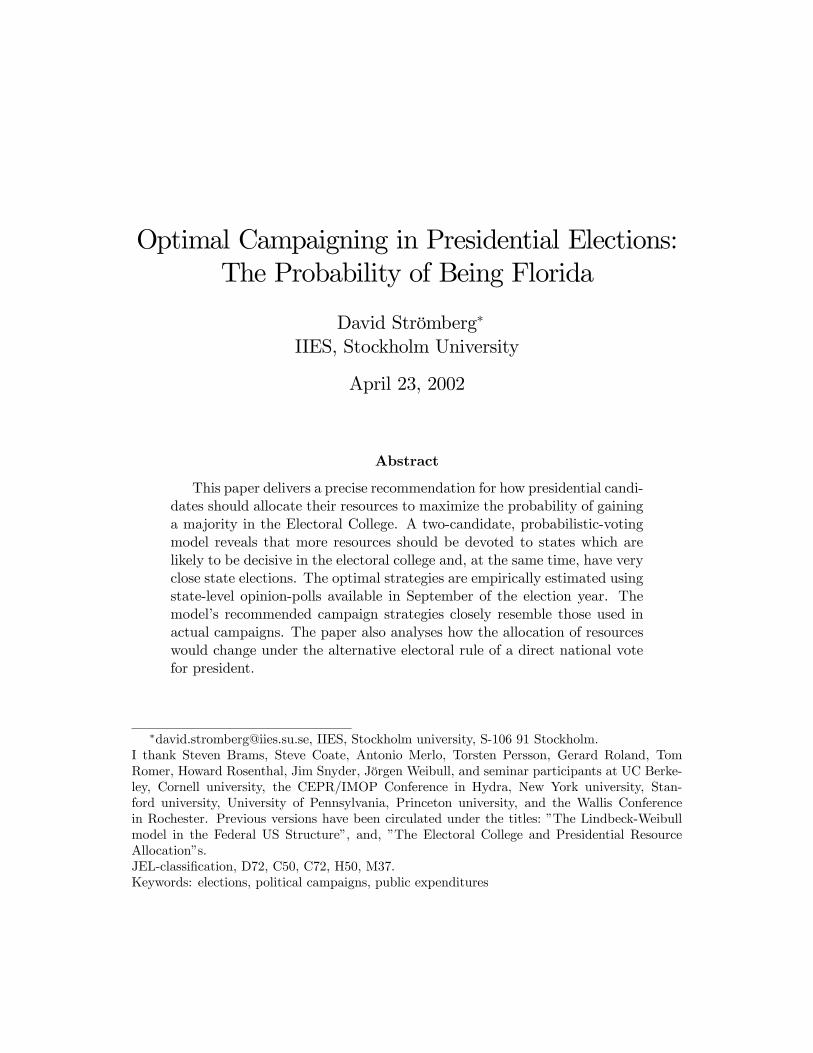
Since the variables determining the allocation under the two systems are dif-ferent, it is not possible on theoretical grounds to determine which system willgenerate more unequal distribution of resources. This will depend on (i) whetherelectoral votes per capita varies more than voter turnout (votes per capita), and(ii) whether the probability of being a decisive swing state per electoral vote variesmore than the share of marginal voters. The left hand plot in Figure 4.1 showsthat Electoral votes per capita million varies more than voter turnout. WhileWyoming has four times as many electoral votes per capita as Texas, Minnesotaonly has 1.7 times as high voter turnout as Hawaii. The right hand plot showsthat the probability of being a decisive swing state per electoral vote varies morethan the share of marginal voters. While Maine is estimated to have twice aslarge a share of marginal voters as California, Michigan has infinitely larger Qs
esthan New York or Texas.Given these results, it is not surprising that the equilibrium allocation of ad-
vertisement expenditures across advertisement markets is much more equal underDirect Vote. This is shown in Figure 4.2.Finally Figure 4.3 shows the per capita weight (Qs respectively Qsv) given to
states under the Electoral College system and the Direct Vote system. Under thepresent system, the allocation of campaign visits and advertisements has beenapproximately proportional to this weight, see Figures 3.1 and 3.3. The scaleon the y-axis is normalized so that 1 represents an equal per capita weight toall states. For example, under the Electoral College, Delaware receives aboutfive times the weight they would receive under equal per capita treatment. New
28
Elec
tora
l vot
es p
er c
apita
M
Voter turnout.38 .641.5
6.0Wyoming
Wisconsin
Minnesota
MaineHawaii
California Qs p
er e
lect
oral
vot
e
Qsv per vote
Michigan
Maine
Massachusetts
California
2.6e-12 5.0e-120
.0016
Figure 4.1: Variables creating unequal distribution under the Electoral Collegeand Direct Vote
Hampshire and New Mexico are also winners under the Electoral College systemwhile states like Texas, Massachusetts and Utah would gain from a reform.Incentives to redistribute campaign resources unequally are much stronger un-
der the Electoral College than under Direct Vote. As I show in Strömberg (2002a),the incentives to allocate federal civilian employment unequally for political pur-poses, are also much stronger under the Electoral College than under Direct Vote.However, these incentives are weaker for federal employment than for campaignexpenditures. The reason is that the uncertainty about the election outcome islarger when decisions about federal employment are taken than during the electioncampaign. Therefore Qs are more evenly distributed across states when relatingto federal employment. As a result, while the principles for political campaigning(studied by Brams and Davis (1974), or Nagler and Leighley (1992)) are the sameas for political distribution of funds (studied by, for example Wright (1974) andWallis (1996)), the optimal allocations are different.Note that Qsv does not measure average ”voting power”, that is, the proba-
bility that an average voter in state s is decisive in the Direct Vote system. Itmeasures the expected number of voters in state s who are decisive and at thesame time swing voters (indifferent between voting for D and R ). In contrast,under the Electoral College, Qs measures ”voting power”. In this model with acontinuum of voters, a vote is decisive when the state is decisive and the stateelection is exactly tied. This implies that while the allocation of resources underthe Electoral College is determined by the ”voting power”, this is not true underDirect Vote.
29

Dire
ct V
ote
Electoral College0 .5 1 1.5 2
0
.5
1
1.5
2
Bangor, ME
Alberqurque-Santa Fe
Figure 4.2: Optimal advertisement expenditures (dollars per capita) by advertise-ment market
12
34
56
0
Texa
sU
tah
Mas
sach
uset
tsId
aho
Kan
sas
Neb
rask
aR
hode
Isla
ndO
klah
oma
New
Yor
kH
awai
iSo
uth
Car
olin
aA
laba
ma
Ver
mon
tM
aryl
and
Sout
h D
akot
aA
lask
aM
aine
Indi
ana
Mon
tana
Nor
th D
akot
aV
irgin
iaN
ew Je
rsey
Illin
ois
Geo
rgia
Cal
iforn
iaN
orth
Car
olin
aW
yom
ing
Min
neso
taA
rizon
aC
onne
ctic
utM
issi
ssip
piW
est V
irgin
iaC
olor
ado
Penn
sylv
ania
Ohi
oW
ashi
ngto
nFl
orid
aK
entu
cky
Loui
sian
aN
evad
aW
isco
nsin
Mic
higa
nTe
nnes
see
Ore
gon
Mis
sour
iA
rkan
sas
Iow
aN
ew M
exic
oN
ew H
amps
hire
Del
awar
e
Electoral College, Qs/ns
Direct Vote, Qsv/ns
Figure 4.3: Treatment under the Electoral College and Direct Vote
30

5. Conclusion
This paper explores how the Electoral College shapes incentives for presidentialcandidates to allocate resources across states. It does so by developing a proba-bilistic voting model of electoral competition under the Electoral College system.The model delivers a precise recommendation for how presidential candidates,trying to maximize the probability of gaining a majority in the Electoral College,should allocate their resources. Basically, more resources should be devoted tostates who are likely to be decisive swing states, that is, states who are decisive inthe electoral college and, at the same time, have very close state elections. Theprobability of being a decisive swing state is fully characterized, both theoretically,and empirically.The theoretical solutions show, first, that the probability of being a decisive
swing state is roughly proportional to the number of electoral votes. Second, thisprobability per electoral vote is highest for states who have a forecasted stateelection outcome which lies between a draw and the forecasted national electionoutcome. For example, suppose that the Democrats are ahead 60-40 in the na-tional polls and in Pennsylvania state polls, while the Texas state polls show adraw. On one hand, candidate visits are more likely to influence the state electionin forecasted swing states like Texas than in states like Pennsylvania. On theother hand, if Texas is still a swing state on election day, then the Democrats areprobably winning by a landslide anyway, while if Pennsylvania is a swing state onelection day, then the election at the national level is likely to be close.The model shows how to strike a balance between high average influence
(Texas) and influence when it matters (Pennsylvania). The more correlated stateoutcomes are, the more attention should be given to states like Pennsylvania.The maximum attention should typically be given to states with polls halfwaybetween a draw and the national polls, around 55-45 in this example. The modelalso shows that candidates who are trailing should try to go for large states wherethey are behind. Even if this decreases the expected number of electoral votesthat the candidate gets, it increases the variance in the outcome and therefore theprobability of winning.The model is applied to presidential campaign visits across states during
the 1988-2000 presidential elections, and to presidential campaign advertisementsacross media markets in the 2000 election. The actual allocation of these resourcesclosely resembles the optimal allocation in the model. In the 2000 election, thecorrelation between optimal and actual visits by state is 0.91, and the correlation
31

between optimal and actual advertisement expenditures by advertising market is0.88.The paper finally analyses how the allocation of advertisements across media
markets would change under an institutional reform, namely the transition to adirect national vote for president. The allocational principles are quite differentunder the two systems, and the incentives to favor certain markets are muchstronger under the electoral college than under the direct vote, causing a moreunequal distribution of resources.
32

References
[1] Anderson, Gary M. and Robert D. Tollison, “Congressional Influence andPatterns of New Deal Spending, 1933-1939”, Journal of Law and Economics,1991, 34, 161-175.
[2] Banzhaf, John R., ”One man, 3.312 votes: a mathematical analysis of theElectoral College”, Villanova Law Review 13, 1968, 304-332.
[3] Brams, Steven J. and Morton D. Davis, ”The 3/2 Rule in Presidential Cam-paigning.” American Political Science Review, March 1974, 68(1), 113-34.
[4] Campbell, James E. (1992). Forecasting the presidential vote in the states.American Journal of Political Science, 36, 386-407.
[5] Chamberlain, Gary, and Michael Rothchild, ”A note on the probability ofcasting a decisive vote”, Journal of Economic Theory 25, 1981, 152-162.
[6] Cohen, Jeffrey E., ”State-level public opinion polls as predictors of Presiden-tial Election Results”, American Politics Quarterly, Apr98, Vol. 26 Issue 2,139.
[7] Colantoni, Claude S., Terrence J. Levesque, and Peter C. Ordeshook, ”Cam-paign resource allocation under the electoral college (with discussion)”, Amer-ican Political Science Review 69, 1975, 141-161.
[8] Gelman, Andrew, and Jonathan N. Katz, ”How much does a vote count?Voting power, coalitions, and the Electoral College”, Social Science WorkingPaper 1121, 2001, California Institute of Technology.
[9] Gelman, Andrew, and Gary King, ”Why are American presidential electioncampaign polls so variable when votes are so predictable?”, British Journalof Political Science, 1993, 23, 409-451.
[10] Gelman, Andrew, Gary King, and W. John Boscardin, ”Estimating the prob-ability of events that have never occurred: when is your vote decisive?”, 1998,Journal of the American Statistical Association, 93(441), 1-9.
[11] Hobrook, Thomas M. and Jay A. DeSart, ”Using state polls to forecast pres-idential election outcomes in the American states”, International Journal ofForecasting, 1999, 15, 137-142.
33

[12] Lindbeck, Assar, Jörgen W. Weibull, ”Balanced-budget redistribution as theoutcome of political competition”, Public Choice, 1987, 52, 273-97.
[13] Lizzeri Allesandro and Nicola Persico, The provision of public goods underalternative electoral incentives, American Economic Review, 91(1), 2001, 225-239.
[14] Merrill, Samuel III, ”Citizen Voting Power Under the Electoral College: AStochastic Voting Model Based on State Voting Patterns”, SIAM Journal onApplied Mathematics, 34(2), 376-390.
[15] Nagler, Jonathan, and Jan Leighley, ”Presidential campaign expenditures:Evidence on allocations and effects”, Public Choice 72, 1992, 319-333.
[16] Persson, Torsten, and Guido Tabellini, ”Political Economics: explaining eco-nomic policy”, MIT Press, 2000.
[17] Persson, Torsten and Guido Tabellini, ”The Size and Scope of Government:Comparative Politics with Rational Politicians,” European Economic Review43, 1999, 699-735.
[18] Rosenstone, Steven J., ”Forecasting presidential elections”, 1983, New Haven:Yale University Press.
[19] Shachar, Ron, and Barry Nalebuff, ”Follow the leader: Theory and evidenceon political participation”, American Economic Review 89(3), 1999, 525-547.
[20] Shaw, Daron R., ”The Effect of TV Ads and Candidate Appearances onStatewide Presidential Votes, 1988-96, American Political Science Review93(2), 1999, 345-361.
[21] Strömberg, ”The Electoral College and the Distribution of Federal Employ-ment”, Stockholm university, 2002a, in preparation.
[22] Strömberg, ”Follow the Leader 2.0: Theory and Evidence on Political Par-ticipation in Presidential Elections”, Stockholm university, 2002b, in prepa-ration.
[23] Snyder, James M., ”Election Goals and the Allocation of Campaign Re-sources”, Econometrica 57(3), 1989, 637-660.
34

[24] Wallis, John J., “What Determines the Allocation of National GovernmentGrants to the States?”, NBER Historical paper 90, 1996.
[25] Wright, Gavin , ”The Political Economy of New Deal Spending: An Econo-metric Analysis”, Review of Economics and Statistics 56, 1974, 30-38.
[26] Holbrook and DeSart, 1999; Rosenstone, 1983).
35

6. Appendix
6.1. Proof of Proposition 1
Symmetry. The best-reply functions of candidates D and R are characterized bythe first order conditions
Qsu0 ¡dDs ¢ = λD,
Qsu0 ¡dRs ¢ = λR.
Therefore,u0¡dDs¢
u0 (dRs )=
λD
λR, (6.1)
for all s. Suppose that dD 6= dR. This means that dDs < dRs for some s, implyingthat λD > λR by equation (6.1). Because of the budget constraint, it must be thecase that dDs0 > d
Rs0 for some s
0, which implies λD < λR, a contradiction. Therefore,λD = λR which implies dDs = d
Rs for all s.
Uniqueness: Suppose there are two equilibria with equilibrium strategies d andd0 corresponding to λ > λ0. The condition on the Lagrange multipliers implies ds >d0s for all s which violates the budget constraint. Therefore, the only possibility isλ = λ0 which implies ds = d0s for all s.
6.2. Non-interior equilibria
A NE¡dD∗, dR∗
¢in the game of maximizing the expected probability of winning
is characterized by
∂PD¡dD∗, dR∗
¢∂dDs
= Qs¡u¡dD∗¢− u ¡dR∗¢¢u0 ¡dD∗s ¢ = Qsu0 ¡dD∗s ¢ = λD, if dD∗s ∈ (0, I] ,
∂PD¡dD∗, dR∗
¢∂dD∗s
= Qsu0 ¡dD∗s ¢ < λD, if dD∗s = 0.
Similarly for R:
∂¡1− PD ¡dD∗, dR∗¢¢
∂dR∗s= Qsu
0 ¡dR∗s ¢ = λR, if dR∗s ∈ (0, I] ,
∂¡1− PD ¡dD∗, dR∗¢¢
∂dR∗s= Qsu
0 ¡dR∗s ¢ < λR, if dR∗s = 0.
36

Suppose λR > λD. First, note that both dR∗s and dD∗s are weakly increasing inQs. Suppose R visits (dR∗s > 0) the x states with the highest Qs and D visits they states with highest Qs. In states which both candidates visit
u0¡dD∗s¢
u0 (dR∗s )=
λD
λR< 1,
so dR∗s < dD∗s . Since D spends more time in all states which both visit, D mustvisit fewer states, and x > y. Therefore, there must be some state s0 which Rvisits but D does not. In this state
λD > Qsu0 (0) > Qsu0
¡dR∗s¢= λR.
But this contradicts the assumption λR > λD. Therefore, non-interior equilibriaare also symmetric, dD = dR. In these equilibria, both candidates make the samenumber of visits to the x states with the highest Qs.
6.3. Derivation of Qs
From Proposition 1,
Qs = Qsµ +Qsσ
= es
Z1
σEϕ (x (η)) gs (−µs − η)h (η) dη
+e2sσ2E
Zϕ (x (η))x (η)
µ1
2−Gs (.)
¶gs (−µs − η)h (η) dη,
where
x (η) =12
Ps es − µσE
.
To see that Qs is approximately the joint probability of a state being decisivein the Electoral College at the same time as having a close election, note thatdisregarding state s0, the electoral electoral vote outcome,
Ps6=s0 Dses, is approx-
imately normally distributed with mean
µ−s0 = µ− esGs (·) (6.2)
and varianceσ2E−s0 = σ2E − e2sGs (·) (1−Gs (·)) . (6.3)
37

The electoral votes of state s0 are decisive ifXs6=s0
Dses ∈µP
sDs2
,
Ps0 Ds2
− es¶.
The probability of this event is approximately
P = Φ
ÃPsDs2− µ−s0
σE−s0
!− Φ
ÃPsDs2− es − µ−s0σE−s0
!.16
First, make a second-order Taylor-expansion of P around the point
x0 (η) =
PsDs2− µ
σE−s0,
so that
P ≈ ϕ (x0)es
σE−s0+
e2sσ2E−s0
ϕ (x0)x0
µGs (·)− 1
2
¶.
Next, given a national shock, η, the probability that the outcome in the state lieswithin two percent of a draw equals
Gs£(−µs − η)− σfsΦ
−1 (.49)¤−Gs £(−µs − η)− σfsΦ
−1 (.51)¤.
To a first-order approximation, this equals:
gs [−µs − η]σfs¡Φ−1 (.51)− Φ−1 (.49)
¢.
Conditional on the national shock, the events that the state has a close electionand that the state is decisive are independent. Therefore the joint probabilityis the product of the two probabilities. The unconditional probability of beingdecisive and having a close election is approximately
σfs¡Φ−1 (.51)− Φ−1 (.49)
¢ ∗Z µϕ (x0)
esσE−s0
+e2s
σ2E−s0ϕ (x0) x0
µGs (·)− 1
2
¶¶gs (−µs − η)h (η) dη
The only difference between the above expression and Qs, apart from the scalefactor for two percent closeness, is that σE has been replaced by the smaller σE−s0.The difference between σE−s0 and σE is small ( typically around one percent).16This way of calculating the probability of being pivotal was developed by Merrill (1978).
38

The values ofQs reported in the paper have been scaled byΦ−1 (.51)−Φ−1 (.49)to be comparable to the simulated values of Section 2.1. In 3.3 percent of the 1million simulated elections, Florida was decisive in the Electoral College and hada state margin of victory of less than 2 percent. The scaled Qs for Florida was3.5 percent. To get the probability that the state margin of victory is within, say1000, votes, Qs should be scaled by Φ−1
³12+ 500
vs
´− Φ−1
³12− 500
vs
´. Using this
formula, the probability of a state being decisive in the Electoral College, and atthe same time having an election result with a state margin of victory less than1000 was 0.00015 in Florida in the 2000 election. The probability that this wouldhappen in any state was .0044. The probability of a victory margin of one vote inFlorida is 0.15 per million, and the probability of this happening in any state is4.4 per million. The state where one vote is most likely to be decisive is Delaware,where it is decisive .4 times in a million elections.To arrive at a simpler form for Qsµ, do a first order Taylor expansion of the
mean of the expected number of electoral votes µ (η) around η = eη for whichµ (eη) = 1
2
Ps es, that is the value of the national shock which makes the expected
outcome a draw. With this approximation
µ (η) =Xs
esGs (−µs − η) ≈ 12
Xs
es − a (η − eη) ,a =
Xs
esgs (−µs − eη) .Since the mean of the electoral votes, µ (η) , is much more sensitive to nationalshocks than is the variance σE (η), the latter is assumed fixed
σ2E (η) = σ2E =Xs
e2sGs (−µs − eη) (1−Gs (−µs − eη)) .Then
1
σE (η)ϕ
µ 12
Ps es − µ
σE (η)
¶≈ 1
σEϕ
µη − eησE/a
¶This approximation is very good. Figure 6.1 shows the true, tfi, and the approx-imated functions, pfi. The values are calculated for an interval of four standarddeviations centered around eη in the 2000 presidential election. We now have
Qsµ ≈ es 1σE
Zϕ
µη − eησE/a
¶gs (−µs − η)h (η) dη.
39

nytt
tfi pfi
-.027613 .101768
.000531
.014273
Figure 6.1:
Integrating over η,
Qsµ ≈ es ω2πexp
Ã−12
σ2seη2 + (σE/a)2 µ2s + σ2 (eη + µs)2σ2sσ
2 + (σE/a)2 σ2 + (σE/a)
2 σ2s
!(6.4)
where
ω2 =
µ1
(σE/a)2 +
1
σ2s+1
σ2
¶−1.
Qsµ may be written as
Qsµ ≈ es ω2πexp
Ã−12
c+ (µs − µ∗s)2eσ2!,
where
µ∗s = −σ2
σ2 + (σE/a)2eη,
and eσ2 = σ2s +1³
1σ2+ 1
(σE/a)2
´ .Qsσ is calculated using numerical integration.
6.4. Regional swings
The model is now extended to allow for regional popularity swings. These swingsare captured by the parameters ηr, ( r = 1, 2, 3, or 4, depending on whether the
40

state is in the Northeast, the Midwest, the South or the West). A voter i in states in region r will vote for D if
∆us = us¡dDs¢− us ¡dRs ¢ ≥ Ri + ηs + ηr + η.
All four regional swing parameters, ηr, are independently drawn from the samenormal distribution with mean zero and variance σ2r.The equilibrium (∆us = 0) election result in one state equals
yst = Fst (−ηst − ηrt − ηt) .
Inverting
Φ−1(yst) = γst = −1
σf
¡µfst + ηst + ηrt + ηt
¢.
This is a hierarchical random-effects model. Assuming that σf = 1, andgiven the national and regional shocks, γst is normally distributed with mean− ¡µfs + ηrt + ηt
¢and variance σ2s. Let h be the probability density function of
γst:
h (γst; ηrt, ηt) =1p2πσ2s
exp
−12
³γsrt +
1σf
¡µfs + ηrt + ηt
¢´2σ2s
.The joint density of state outcomes (there are Sr states in region r), equals
h (γ) =
Z ∞
−∞
ÃRYr=1
Z ∞
−∞
SrYs=1
h (γst; ηrt, ηt) gr (ηrt) dηrt
!h (ηt) dηt.
The parameters are estimated using maximum likelihood estimation. As re-ported in the main text, the estimated state and national level shock variances aresimilar to those estimated without allowing for regional shocks, σs,post1984 = 0.084,and σ = 0.038. The standard deviation of the regional shock is σr = 0.054 beforestate level forecasts were available in 1988. However, after 1988, the standarddeviation of the regional shocks is zero. Taking into account the information ofSeptember state-level opinion polls, there are no significant regional swings.Even though there were no significant regional shocks in this case, it is interest-
ing to know how the equilibrium would change with regional shocks. Conditional
41

on the national and regional shocks, the state outcomes within each region are in-dependent. Using the Central Limit Theorem for all outcome states within regionr,
Pr
ÃSrXs=1
Dsresr ≤ x | ηr, η!≈ Φ
µx− µrσ2Er
¶,
where
µr = µr¡dD, dR, ηr, η
¢=
SrXs=1
esrGsr (∆usr − µsr − ηr − η) ,
σ2Er = σ2Er¡dD, dR, ηr, η
¢=
SrXs=1
e2srGsr (·) (1−Gsr (·)) .
To estimate the distribution of electoral votes, independent of the regional shocks,do a Taylor-expansion of µr around µ
¡dD, dR, ηr = 0, η
¢, and assume σ2Er =
σ2Er¡dD, dR, ηr = 0, η
¢:
Pr
ÃSrXs=1
Dsresr ≤ x | η!
≈Zηr
Φ
Ãx−PSr
s=1 esrGsr (∆usr − µsr − η) + arηrσEr
!g (ηr) dηr
= Φ
x− µsrqσ2Er + a
2rσ2r
,where
ar =SrXs=1
esrgsr (∆usr − µsr − η) .
So the regional election outcome is approximately normally distributed with mean
µsr =SrXs=1
esrGsr (∆usr − µsr − η) ,
and varianceσ2Er + a
2rσ2r.
42

The total election outcome, the sum of the regional outcomes, is normallydistributed with mean and variance
µ = µ¡dD, dR, η
¢=
RXr=1
SrXs=1
esGs (∆us − µs − η) =SXs=1
esGs (∆us − µs − η) ,
σ2E = σ2¡dD, dR, η
¢=
RXr=1
¡σ2Er + a
2rσ2r
¢=
SXs=1
e2sGs (·) (1−Gs (·)) +RXr=1
ÃSrXs=1
esgs (∆us − µs − η)
!2σ2r.
The mean is the same as without regional swings. However, allowing for regionalcorrelation increases the variance in the electoral vote outcome, σ2E. This will havetwo effects. Most importantly, Qs becomes less sensitive to vote shares, as thevariance of the normal form curve of Figure 2.3 increases. Therefore it becomesmore important to visit large states, such as California, rather than states wherethe outcome is close to 50.8 percent. Secondly, it becomes more important tobe close to 50 percent relative to the national shock. This is apparent fromthe mathematical expressions for the mean and variance of that distribution, seeequation (2.10), and footnote (4).
6.5. Campaign advertisements
This Appendix analyses the decision of presidential candidates to allocate adver-tisements across media markets.Two presidential candidates: R and D, select thenumber of ads, am, in each media market m subject to
MXm=1
pmdJm ≤ I,
J = R,D. Media market m contains a mass vms of voters in state s. Voters areaffected by campaign advertisements as captured by the function w(am). A voteri in media market m in state s will vote for D if
∆wm = w¡aDm¢− w ¡aRm¢ ≥ Ri + ηs + η.
In each media market m in state s, the individual specific preferences for can-didates, Ri, are distributed with cumulative density function Fs. The state andnational-level popularity-swings are drawn from the same distributions as before.
43

The share D votes in media market m in state s equals
Fs(∆wm − ηs − η).
D wins the state if Xm
vmsFs(∆wm − ηs − η) ≥ vs2.
Define the total (state and national) swing which causes a draw in the state:
ηs¡aD, aR
¢:Xm
vmsFs(∆wm − ηs¡aD, aR
¢) =
vs2. (6.5)
D wins state s ifηs + η ≤ ηs
¡aD, aR
¢.
Conditional on the aggregate shock η, and the platforms, aD, and aR, this happenswith probability
Gs¡ηs¡aD, aR
¢− η¢.
The function ηs¡aD, aR
¢now plays the same role as∆us in Section 2, see equation
(2.2). The rest of the analysis is in that section, only exchanging ηs¡aD, aR
¢for
∆us. The best reply functions of D is characterized by
SXs=1
Qs
MXm=1
∂ηs¡aD, aR
¢∂aDc
= λDpm. (6.6)
Similarly, the best reply function of R is characterized by equation (6.6), replacingsuperscripts D by R. Because of the fixed budget constraint, the allocations mustbe symmetric, λD = λR = λ. Differentiating equation (6.5), and evaluating it inequilibrium yields
∂ηs¡aD, aR
¢∂aDm
=vmsvsw0¡aDm¢.
Proposition 3. A pair of strategies for the parties¡aD, aR
¢that constitute a NE
in the game of maximizing the expected probability of winning the election mustsatisfy aD = aR = a∗, and for all s and for some λ > 0
Qmw0 (a∗m) = λpm, (6.7)
where
Qm =SXs=1
Qsvmsvs.
44

Qm is the sum of the Qs of the states in the media market weighted by the shareof the voting population of state s that lives in media market m.Last, assuming that votes per capita
vmsnms
= ts
is the same for all media markets within each state,
Qm =SXs=1
Qsnmsns.
6.6. Visits to media markets
One possible objection is that candidates do not choose which states to visit, butrather which media markets. Suppose that instead of buying ads, the candidatescan decide which media markets to visit. A voter i in media market m in state swill vote for D if
∆um = u¡dDm¢− u ¡dRm¢ ≥ Ri −Di + ηs + η.
This model is the same as the advertising model with the same price for a visit,pm = 1, in all media markets. The equilibrium condition is
u0 (d∗m)Qm = λ. (6.8)
To compare this allocation to the optimal allocation when the state was theunit of analysis, the visits to a media market was distributed across states accord-ing to the share of the media market population that lives in that state:
eds =Xm
nmsnm
d∗m.
Qm and eds were calculated using data on the 75 largest Designated Market Ar-eas (DMA’s) used by Nielsen Media Research. A DMA consists of all countieswhose largest viewing share is given to stations of that same market area. Non-overlapping DMA’s cover the entire continental United States, Hawaii and partsof Alaska. The resulting allocation of visits to media markets, distributed acrossstates, is shown in Figure 6.2, and compared to the equilibrium visits to states.
45

0 2 4 6 8 10 12
Massachusetts
Kansas
Nebraska
Idaho
D.C.
Utah
Rhode Island
Texas
Oklahoma
New York
Hawaii
Vermont
South Carolina
Alaska
Alabama
South Dakota
North Dakota
Montana
Maine
Wyoming
Maryland
Indiana
West Virginia
Virginia
Mississippi
Connecticut
Delaware
New Jersey
Minnesota
Nevada
Arizona
New Hampshire
Georgia
New Mexico
North Carolina
Colorado
Arkansas
Kentucky
Iowa
Illinois
Oregon
Louisiana
Washington
Wisconsin
Tennessee
Missouri
Ohio
California
Pennsylvania
Michigan
Florida
State visitsMedia market visits
Figure 6.2: Visits to media markets, allocated across states
46

The resulting allocations are quite similar. Since media markets cross stateborders, there are spillovers. This is why New York and Massachusetts receivemore visits, and New Hampshire less, if candidates target media markets. Second,states which are more difficult to cover receive more visits. To get the intuition,consider two identical states, except that one is covered by a single media marketand the other by two of equal size. Suppose both candidates make four visits toeach state: in the state with two media markets they visit both markets twice.In this case, the marginal impact of a visit on the probability of winning mustbe higher in the state with the two media markets. In this state each voter hasonly seen the candidates twice while each voter in the other state has seen thecandidate four times.It may also be interesting to know the average number of times people living
in a state get the chance to see the candidates. The number of equilibrium visitsto an average media market in state s is
ds =Xm
nmsnsd∗m.
This is highest in Delaware, Michigan, and Pennsylvania. Because of its manymedia markets, Florida only comes in eighth place.
6.7. Direct presidential vote
The mean outcome in state s is
µvs¡zL, zR, η
¢=
ZFs(∆us − η − ηs)gs (ηs) dηs
= Φ
∆us − η − µsqσ2s + σ2fs
.17The expression for the variance in one state is, by definition,
σ2vs = v2s
Z Φ
µ∆us − η − ηs − µs
σfs
¶− Φ
∆us − η − µsqσ2s + σ2fs
2
gs (ηs) dηs,
17This is not completely trivial. Contact the author for details.
47

and the total variance isσ2v =
Xs
σ2vs.
The probability of D winning the election is
PD¡zD, zR
¢= 1−
ZΦ
µ 12
Ps vs − µvσv
¶h (η) dη.
where:
µv =Xs
vsΦ
∆us − µs − ηqσ2s + σ2fs
, (6.9)
σ2v = σ2v (∆us, η) .
The derivative of PD¡zD, zR
¢with respect to ∆us equals
Qsv = Qsvµ +Qsvσ,
where
Qsvµ =vs
σvq
σ2s + σ2fs
Zϕ
µ 12
Ps vs − µvσv
¶ϕ
∆us − µs − ηqσ2s + σ2fs
h (η) dη,Qsvσ =
1
σv
Zϕ
µ 12
Ps vs − µvσv
¶µ 12
Ps vs − µvσv
¶∂σv∂∆us
h (η) dη,
and
∂σ2v∂∆us
= 2v2s
Z Φ
µ∆us − η − ηs − µs
σfs
¶− Φ
∆us − η − µsqσ2s + σ2fs
1
σfsϕ
µ∆us − η − ηs − µs
σfs
¶− 1q
σ2s + σ2fs
ϕ
∆us − η − µsqσ2s + σ2fs
gs (ηs) dηsUsing this information, Qsvµ may be calculated either using the same type ofapproximation as used for Qsµ, or by numerical integration. The second term,
48

Qsvσ, is calculated by numerical integration. However, it turns out that this effectis negligible compared to Qsvµ.The interpretation of Qsvµ is the following. Conditional on η, the expected
number of swing voters is
vs
Z ∞
−∞fs(∆us − η − ηs)gs (ηs) dηs =
vsqσ2s + σ2fs
ϕ
∆us − µs − ηqσ2s + σ2fs
.and the likelihood of a tie is
1
σvϕ
µ 12
Ps vs − µvσv
¶.
Therefore, the unconditional expected number of swing voters in case of a tie is
vs
σvq
σ2s + σ2fs
Zϕ
µ 12
Ps vs − µvσv
¶ϕ
∆us − µs − ηqσ2s + σ2fs
h (η) dη,which is the same as Qsvµ.
6.8. Is the electoral vote outcome normally distributed?
This appendix plots the distributions of election outcomes for all elections 1948-2000, with and without using the asymptotic normal distribution. To avoid nu-merical integration over η, the following extra approximation is exploited. Usingthe asymptotic distribution, the approximate probability of D vote share higherthan Vs is Z
1− Φ
µVs − µσE
¶h (η) dη
µ ≈ µ (η = 0)−Xs
esgs (−µs) η
≈Z1− Φ
µVs − µ (0) + aη
σE
¶h (η) dη = 1−
ZΦ
µη + 1
a(Vs − µ (0))σE/a
¶h (η) dη
= 1− Φ
1a(Vs − µ (0))q(σE/a)
2 + σ2
= Φ
ÃVs − µ (0)pσ2E + a
2σ2
!.
49
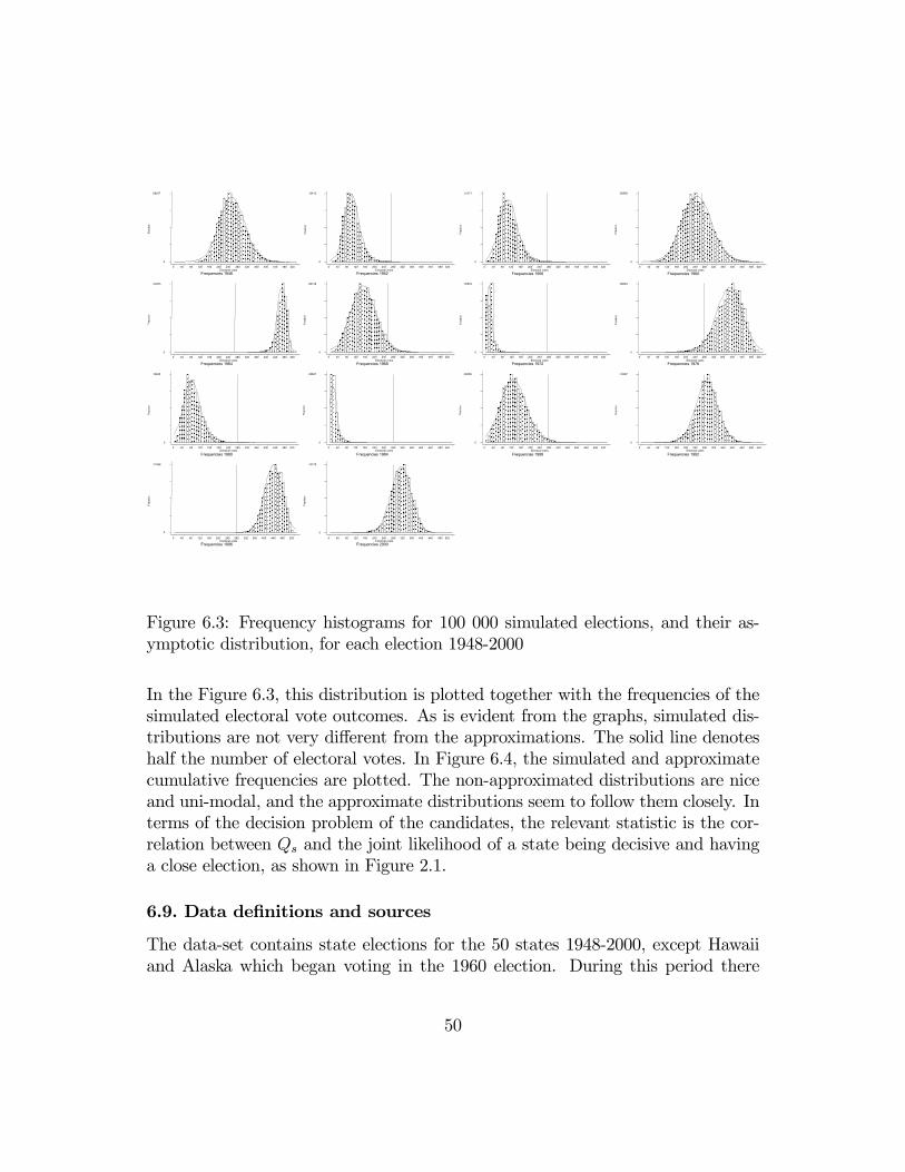
Frac
tion
Frequencies 1948Electoral votes
0 40 80 120 160 200 240 280 320 360 400 440 480 520
0
.08247
Frac
tion
Frequencies 1952Electoral votes
0 40 80 120 160 200 240 280 320 360 400 440 480 520
0
.13412
Frac
tion
Frequencies 1956Electoral votes
0 40 80 120 160 200 240 280 320 360 400 440 480 520
0
.12171
Frac
tion
Frequencies 1960Electoral votes
0 40 80 120 160 200 240 280 320 360 400 440 480 520
0
.06958
Frac
tion
Frequencies 1964Electoral votes
0 40 80 120 160 200 240 280 320 360 400 440 480 520
0
.23055
Frac
tion
Frequencies 1968Electoral votes
0 40 80 120 160 200 240 280 320 360 400 440 480 520
0
.08149
Frac
tion
Frequencies 1972Electoral votes
0 40 80 120 160 200 240 280 320 360 400 440 480 520
0
.35533
Frac
tion
Frequencies 1976Electoral votes
0 40 80 120 160 200 240 280 320 360 400 440 480 520
0
.08083
Frac
tion
Frequencies 1980Electoral votes
0 40 80 120 160 200 240 280 320 360 400 440 480 520
0
.12925
Frac
tion
Frequencies 1984Electoral votes
0 40 80 120 160 200 240 280 320 360 400 440 480 520
0
.35827
Frac
tion
Frequencies 1988Electoral votes
0 40 80 120 160 200 240 280 320 360 400 440 480 520
0
.08358
Frac
tion
Frequencies 1992Electoral votes
0 40 80 120 160 200 240 280 320 360 400 440 480 520
0
.10087
Frac
tion
Frequencies 1996Electoral votes
0 40 80 120 160 200 240 280 320 360 400 440 480 520
0
.11068
Frac
tion
Frequencies 2000Electoral votes
0 40 80 120 160 200 240 280 320 360 400 440 480 520
0
.10178
Figure 6.3: Frequency histograms for 100 000 simulated elections, and their as-ymptotic distribution, for each election 1948-2000
In the Figure 6.3, this distribution is plotted together with the frequencies of thesimulated electoral vote outcomes. As is evident from the graphs, simulated dis-tributions are not very different from the approximations. The solid line denoteshalf the number of electoral votes. In Figure 6.4, the simulated and approximatecumulative frequencies are plotted. The non-approximated distributions are niceand uni-modal, and the approximate distributions seem to follow them closely. Interms of the decision problem of the candidates, the relevant statistic is the cor-relation between Qs and the joint likelihood of a state being decisive and havinga close election, as shown in Figure 2.1.
6.9. Data definitions and sources
The data-set contains state elections for the 50 states 1948-2000, except Hawaiiand Alaska which began voting in the 1960 election. During this period there
50

Cumulative distribution 1948Electoral votes
cum approx
0 40 80 120 160 200 240 280 320 360 400 440 480 520
.001
1
Cumulative distribution 1952Electoral votes
cum approx
0 40 80 120 160 200 240 280 320 360 400 440 480 520
.001
1
Cumulative distribution 1956Electoral votes
cum approx
0 40 80 120 160 200 240 280 320 360 400 440 480 520
.001
1
Cumulative distribution 1960Electoral votes
cum approx
0 40 80 120 160 200 240 280 320 360 400 440 480 520
.001
1
Cumulative distribution 1964Electoral votes
cum approx
0 40 80 120 160 200 240 280 320 360 400 440 480 520
4.3e-07
1
Cumulative distribution 1968Electoral votes
cum approx
0 40 80 120 160 200 240 280 320 360 400 440 480 520
.001
1
Cumulative distribution 1972Electoral votes
cum approx
0 40 80 120 160 200 240 280 320 360 400 440 480 520
.001
1
Cumulative distribution 1976Electoral votes
cum approx
0 40 80 120 160 200 240 280 320 360 400 440 480 520
.000506
1
Cumulative distribution 1980Electoral votes
cum approx
0 40 80 120 160 200 240 280 320 360 400 440 480 520
.001
1
Cumulative distribution 1984Electoral votes
cum approx
0 40 80 120 160 200 240 280 320 360 400 440 480 520
.001
1
Cumulative distribution 1988Electoral votes
cum approx
0 40 80 120 160 200 240 280 320 360 400 440 480 520
.001
1
Cumulative distribution 1992Electoral votes
cum approx
0 40 80 120 160 200 240 280 320 360 400 440 480 520
.000321
1
Cumulative distribution 1996Electoral votes
cum approx
0 40 80 120 160 200 240 280 320 360 400 440 480 520
.001
1
Cumulative distribution 2000Electoral votes
cum approx
0 40 80 120 160 200 240 280 320 360 400 440 480 520
.000229
1
Figure 6.4: Simulated and asymptotic cdf, 100 000 simulated elections, for eachelection 1948-2000.
51

were a total of 694 state-level presidential election results. Of this total, 13 stateelections were excluded, leaving a total of 681 observations. Four elections inAlaska and Hawaii were excluded because there were no lagged vote returns. Nineelections are omitted because of idiosyncracies in Presidential voting in Alabamain 1948, and 1964, and in Mississippi in 1960; see Campbell 1992.
• Dmvote: state Democratic percentage of the two-party presidential vote.Source: 1940-1944, ICPSR Study 0019; 1948-1988, Campbell; 1992, 1996,Statistical Abstract of the United States 2000; 2000, Federal Election Com-mission, 2000 OFFICIAL PRESIDENTIAL GENERAL ELECTION RE-SULTS.
• Electoral votes won (by state). Source: National Archives and RecordsAdministration.
• National trial-heat poll results. Source: 1948-1996, Campbell (2000); 2000,Gallup.
• Second quarter national economic growth, multiplied by 1 if Democraticincumbent president and -1 if Republican incumbent president. Source:August or September election year issue of the Survey of Current Business,U.S. Department of Commerce, Bureau of Economic Analysis.
• Growth in personal state’s total personal income between the prior year’sfourth quarter and the first quarter of the election year, standardized acrossstates in each year, multiplied by 1 if Democratic incumbent president and-1 if Republican incumbent president. Source: Survey of Current Business,U.S. Department of Commerce, Bureau of Economic Analysis.
• Incumbent: 1 if incumbent president Democrat, -1 if incumbent presidentRepublican.
• Presinc: 1 if incumbent Democratic president seeking re-election, -1 if in-cumbent Republican president seeking re-election.
• President’s home state: 1 if Democratic president home state, -1 if Repub-lican (0.5 and -0.5 for large states (New York, Illinois, California). Source:Campbell 1948-1988; 1992-2000: Dave Leip’s Atlas of U.S. Presidential Elec-tions.
52

• Vice president’s home state: 1 if Democratic president home state, -1 ifRepublican (0.5 and -0.5 for large states (New York, Illinois, California).Source: Campbell 1948-1988; 1992-2000: Dave Leip’s Atlas of U.S. Presi-dential Elections.
• Average ADA-scores: Average ADA-scores of state’s members in Congressyear before election. Source: Tim Groseclose(http://faculty-gsb.stanford.edu/groseclose/homepage.htm).
• Legis: Partisan division of the lower chamber of the state legislature afterthe previous midterm election. Index is Democratic share of state legisla-tive seats above the 50% mark. Two states, Nebraska and Minnesota, heldnonpartisan state legislative elections for all (Nebraska) or part (Minnesotaof the period under study. In the case of Nebraska, the state legislative di-vision was estimated based on the ranking of states of Wright, Erikson, andMcIver’s state partisan rankings based on public opinion data. Using thisindex, Nebraska was assigned the mean partisan division of the state mostsimilar to it on the public opinion index, the nearly equally Republican stateof North Dakota. The partisan division of the Minnesota legislature in itsnonpartisan years (before 1972) is coded as the mean of its partisan divisiononce it reformed to partisan elections (62% Democratic). Washington D.C.was as having the same partisan division as Maryland. Source: 1948-1988,Campbell; 1992-2000, Statistical Abstract of the United States.
• State-level opinion polls. Democratic share of two party vote. Source: Pre-election issues of the Hotline (www.nationaljournal.com).
• Regional dummy variables, see Campbell.• Participation rate: 1948-1988, Shachar and Nalebuff (1999), voting age pop-ulation 1992-2000, and votes cast 2000, Federal Election Commission, votescast 1992, 1996, Statistical Abstract of the United States.
53

Table 1. Dependent variable: γst , Φ-1(democratic share of two-party vote)
National variables:Opinion poll 0.453
(0.053)
Second quarter economic growth 0.064(0.010)
Incumbent president running for re-election 0.053(0.023)
Incumbency -0.036(0.018)
Constant -0.049(0.010)
State variables, 1948-1984Lagged democratic share of two-party vote, 0.266difference from national mean (0.032)
Twice lagged democratic share of two-party vote, 0.216difference from national mean (0.025)
Home state of presidential candidate 0.175(0.028)
Home state of vice presidential candidate 0.056(0.023)
First quarter state economic growth. 0.017(0.005)
Average ADA-scores 0.0021(0.0003)
Democratic vote-share in midterm state legislative election 0.020(0.007)
State variables, 1988-2000Lagged democratic share of two-party vote, 0.515difference from national mean (0.081)
Twice lagged democratic share of two-party vote, 0.074difference from national mean (0.070)
Average ADA-scores 0.0009(0.0004)
State-level opinion poll 0.389(0.050)
σ 0.033(0.007)
σs1948-1984 0.102(0.003)
σs1948-1984 - σs1988-2000 0.025(0.005)
Average prediction error (percentage points) 3.0
Number of observations 681

SEMINAR PAPER SERIES The Series was initiated in 1971. For a complete list of Seminar Papers, please contact the Institute. 2000 681. Lars E.O. Svensson: The First Year of the Eurosystem: Inflation Targeting or Not?
11 pp. 682. Jonas Agell and On the Analytics of the Dynamic Laffer Curve. 25pp. Mats Persson: 683. Harry Flam and EMU Effects on International Trade and Investment. 42 pp. Per Jansson: 684. Harry Flam and The Young Ohlin on the Theory of "Interregional and Inter-
M. June Flanders: national Trade". 18 pp. 685. Assar Lindbeck: Pensions and Contemporary Socioeconomic Change. 27 pp. 686. Mats Persson: Five Fallacies in the Social Security Debate. 16 pp. 687. Lars E.O. Svensson: The Zero Bound in an Open Economy: A Foolproof Way of
Escaping from a Liquidity Trap. 44 pp. 688. Lars E.O. Svensson and Indicator Variables for Optimal Policy. 43 pp. Michael Woodford: 2001 689. Lars E.O. Svensson and Indicator Variables for Optimal Policy under Assymetric Michael Woodford: Information. 690. Lars Calmfors Wages and Wage-Bargaining Institutions in the EMU - A
Survey of the Issues. 691. Assar Lindbeck and Raising Children to Work Hard: Altruism, Work Norms and Sten Nyberg Social Insurance. 692. Lars Calmfors and Unemployment Benefits, Contract Length and Nominal Wage Åsa Johansson Flexibility. 693. Peter Svedberg Undernutrition Overestimated. 694. Assar Lindbeck Changing Tides for the Welfare State. 695. Antoni Calvó-Armengol and Job Matching, Social Network and Word-of-Mouth
Yves Zenou Communication. 696. Mats Persson and Incentive and Incarceration Effects in a General Equilibrium

Claes-Henrik Siven Model of Crime. 697. Magnus Henrekson and The Effects on Sick Leave of Changes in the Sickness Insurance Mats Persson System. 698. Peter Svedberg Income Distribution Across Countries: How Is it Measured and
What Do the Results Show? 2002 699. Peter Svedberg Hunger in India – Facts and Challenges. 700. Lars Calmfors, Does Active Labour Market Policy Work? Lessons from the Anders Forslund, and Swedish Experiences. Maria Hemström. 701. Kjetil Storesletten Fiscal Implications of Immigration. 702. Kjetil Storesletten, Consumption and Risk Sharing over the Life Cycle. Chris Telmer, and Amir Yaron 703. Kjetil Storesletten, Asset Pricing with Idiosynchratic Risk and Overlapping Chris Telmer, and Generations. Amir Yaron 704. John Hassler, The Survival of the Welfare State. José V. Rodriguez Mora, Kjetil Storesletten, and Fabrizio Zilibotti 705. John Hassler, A Positive Theory of Geographical Mobility and Social José V. Rodriguez Mora, Insurance. Kjetil Storesletten, and Fabrizio Zilibotti 706. David Strömberg Optimal Campaigning in Presidential Elections: The Probability
of Being Florida.
ISSN 0347-8769 Stockholm, 2002 Institute for International Economic Studies