Optimal Contracting with Altruistic Agents:

A Structural Model of Medicare Reimbursements for Dialysis Drugs

Martin Gaynor∗, Nirav Mehta∗∗, and Seth Richards-Shubik∗∗∗

Carnegie Mellon and NBER∗, Western Ontario∗∗, Lehigh and NBER∗∗∗

March 5, 2018

PRELIMINARY—PLEASE DO NOT CITE

Abstract

We study physician agency and optimal payment policy in the context of an ex-pensive medication (epoetin alfa) used with dialysis. Using Medicare claims data weestimate a model of treatment decisions, in which physicians are partially altruisticand value both their own compensation and their patients’ health. We then use therecovered parameters of the model in combination with results from contract theory toderive and simulate optimal linear and nonlinear reimbursement schedules. Compar-ing outcomes under these optimal contracts against those observed under the actualcontracts suggests that substantial improvements in payment policy can be achievedwithin a fee-for-service framework.

1 Introduction

A central problem in health economics, and in health care organizations, is how to com-

pensate physicians for their services. Physicians are typically viewed as imperfect agents for

their patients, deriving utility from both their private benefits and costs and from the impact

of their services on patient health. A substantial theoretical literature in health economics

considers how these partially altruistic agents might behave under various payment systems,

and a related empirical literature examines how physicians respond to financial incentives.

We extend this work by specifying and estimating a physician utility function that depends

on patient health and physician income, thereby quantifying the level of altruism among

physicians in our setting. We then use the recovered parameters of this utility function

in combination with results from contract theory to derive and simulate optimal payments

to physicians for service provision. Comparing the optimal contract with actual contracts

suggests tractable improvements in payment policy.

1

Our empirical analysis is on the provision of an expensive and controversial medication

used by dialysis centers to treat anemia in patients with end stage renal disease (ESRD). The

medication, epoetin alpha (or “EPO”), was the largest single drug expenditure in Medicare

for several years. Medicare is the predominant payer for the treatment of ESRD in the

United States (at any age), and we use Medicare claims data from 2008 and 2009 to estimate

our model. In the model, physicians choose the quantity of treatment to provide to each

patient, based on the predicted health impact, the cost of treatment, and the payment

contract. Uniquely in our setting, a quantitative measure of patient need is available in the

claims records because providers were required to report a blood measurement in order to be

reimbursed for EPO. The revealed weight placed on improvements in patient health relative

to the physician’s private marginal benefit is our measure of altruism. This parameter and

the other parameters of our model are recovered in a simple manner from the coefficients of

a linear fixed effects regression.

We then address the agency problem that arises when physicians are heterogeneous in

their cost of providing treatment.1 Using the estimated physician utility function, we derive

both optimal (constrained) linear and unconstrained (potentially nonlinear) payment con-

tracts. These contracts are fairly straightforward to construct from the output of the fixed

effects regression. We then compare the reimbursement schedules and induced treatments

under these contracts against the observed outcomes. Preliminary results suggest that the

historical reimbursement rates for EPO were supra-optimally high, and by a wide margin.

This is intuitive, as physician altruism and cost heterogeneity, neither of which may have

been accounted for by the government, both reduce the per-unit payment in the optimal

linear contract. We derive optimal reimbursement rates in the linear contract that are 30

percent lower than the actual rates used by Medicare in 2008 and 2009. The optimal nonlin-

ear contract improves outcomes further, notably by reducing medically unjustified variation

in treatment intensities while also decreasing total expenditures. A simulation for patients

with anemia at the median level of severity finds that the standard deviation of dosages falls

by 70 percent while the mean payment decreases by 40 percent.

1.1 Related literature

We view our paper as being closely related to two literatures described below.

1There are substantial differences across providers in the acquisition cost of the drug, as documented inMedicare renal dialysis facility cost reports (see Section 3). We plan on extending our approach to considerboth cost and altruism heterogeneity in a future version. The optimal nonlinear contract in the case ofmultidimensional heterogeneity is more difficult to characterize than that for the case of one-dimensionalheterogeneity because physician “types” can no longer be ordered, as they can be in the one-dimensionalcase (see (Maskin et al., 1987; Wilson, 1993; Deneckere and Severinov, 2015)).

2

Health economics: There is a rich theoretical literature on physician agency; much of this

literature is discussed in McGuire (2000) and Chalkley and Malcomson (2000). Ellis and

McGuire (1986) provide a seminal contribution. They model physicians as partially altruistic

(imperfect agents) and show that partial cost reimbursement can improve outcomes when

physicians are imperfect agents for their patients and inputs are noncontractible.

By contrast, there are relatively few theoretical papers on optimal contracting in health

care. Chalkley and Malcomson (1998) characterize optimal contracts when patient demand

does not reflect quality, and show that the optimal contract differs depending on the degree

of physician altruism. De Fraja (2000) studies optimal contracts when there is heterogeneity

in physician costs. Jack (2005) allows for heterogeneity in physician altruism and solves for

the optimal contract in an environment where quality is noncontractible. Malcomson (2005)

examines optimal contracts when providers are better informed than purchasers, with no

provider altruism. Chone and Ma (2011) also study how physician altruism may affect the

design of optimal payment schemes.

There is also an empirical literature studying how physicians respond to incentives and

other changes in the environment. Gaynor and Pauly (1990) is an early paper showing that

physicians respond strongly to financial incentive. Chandra et al. (2012) review the literature

studying determinants of physician treatment choices. One determinant they focus on is

physician altruism. Gaynor et al. (2004) specify and estimate a structural model of physician

treatment choice where physicians are partially altruistic. Godager and Wiesen (2013) use

data obtained from a laboratory experiment to document the existence of physician altruism,

which they find to be heterogeneous. Clemens and Gottlieb (2014) examine the impact of

financial incentives in Medicare payment for physicians and find substantial effects on supply,

technology adoption, and patient outcomes.

Our model contains many components of the above literature. The basic model of physi-

cian utility is very similar to that in Gaynor et al. (2004), but allows for cost heterogeneity

as well as altruism. De Fraja (2000) and Jack (2005), noted above, address heterogeneity

across physicians, although there are various distinctions between their models and ours.2

Like Clemens and Gottlieb (2014), we examine the impact of Medicare payment incentives,

although they look at payment incentives broadly, as opposed to our focus on a very specific

program and treatment decision. Last, in contrast to the existing empirical literature, we

not only estimate a model of physician treatment choices and recover physician altruism,

we also empirically characterize the optimal contract and compare it to the actual contracts

used in this context.

2For example, Jack (2005) uses a model with unobserved effort while in our setting the most relevantaspect of the treatment is observed (i.e., the dosage of the drug).

3

Empirical contracts: As Chiappori and Salanie (2003) discuss, there is empirical work

testing for the existence of salient features for the design of optimal contracts (e.g., Chiap-

pori et al. (2006) test for asymmetric information), but there is little work specifying and

estimating structural models and using them to derive optimal contracts. This matters be-

cause the insights from the literature on contracts are most useful when applied in designing

optimal policies that could be implemented in reality.

To the best of our knowledge, there is no work that structurally estimates a model

of physician treatment choices in a principal-agent, or asymmetric information, framework

and uses this to characterize optimal contracts. A handful of papers estimate asymmetric

information models in other settings. For example, Einav et al. (2010) discuss the small

literature doing this for insurance contracts. Paarsch and Shearer (2000) characterize the

optimal linear contract in a hidden action environment. Gayle and Miller (2009) also

study hidden action models, quantifying the welfare loss from moral hazard. In contrast, we

study a screening, or hidden information, model and flexibly characterize the optimal wage

schedule. Screening models, with their focus on unobserved heterogeneity, are clearly policy

relevant.

There is a fairly rich literature on optimal regulation, which considers screening models

in institutional contexts that differ from ours in important ways. Wolak (1994) develops

and estimates a model in which a principal seeks to regulate public utilities of (potentially)

hidden types. Data limitations, including a lack of variation in regulatory regime, mean

the distribution of types cannot be estimated without imposing optimality of the observed

contract. Gagnepain and Ivaldi (2002), study a similar environment, but exploit variation in

the regulatory regime to estimate a parametric distribution of types without having to assume

optimality of the observed contract. This allows them to test whether the observed contract

is optimal. Abito (2017) extends this approach to study optimal pollution regulation. As

in the latter two articles, our setting and data allow us to estimate structural parameters,

including agent types, without imposing optimality of the observed contract. We allow for

a fully flexible type distribution, which is made possible by variation in the observed regime

(i.e., reimbursement contract) and a large number of repeated measures of physicians, as each

physician chooses a treatment choice for each patient they see, under a variety of observed

reimbursement rates.

1.2 Institutional background

ESRD, or kidney failure, is a chronic and life-threatening condition that affects over half a

million individuals in the United States at a given point in time. Since 1973, the Medicare

4

program has provided universal coverage for the treatment of ESRD, regardless of age.

In 2009 Medicare spent $28 billion on health care for individuals with ESRD, and of that

amount, $1.74 billion went to payments for the drug EPO.3 The drug is used to treat anemia,

a lack of red blood cells, which often accompanies chronic kidney disease.4 It is similarly

used to treat anemia in chemotherapy patients. EPO stimulates red blood cell production,

and dialysis providers administer it to their patients to try to maintain a certain level of red

blood cells. The level is commonly measured as hematocrit, which is the volume percentage

of red blood cells in the blood.

Medicare’s payment policy for EPO was debated throughout the 1990s and 2000s, largely

because of concerns that the reimbursement rates were too generous and encouraged over-

provision. While dialysis itself was reimbursed with a prospective payment system (PPS)

known as the “composite rate,” EPO was a separately billable drug with its own per-unit

reimbursement rate. Prior to 2005, the rate was held fixed at $10.00 per 1000 units. In

2006, Medicare adopted a new policy where the reimbursement rate was based on average

sales prices calculated from data reported by the drug manufacturer. This policy, which

was in effect through 2010 (including the years we use to estimate provider behavior), set a

reimbursement rate each quarter equal to 106 percent of the national average sales price from

roughly six months earlier (GAO, 2006). Later, in 2011, Medicare adopted a comprehensive

“bundled” PPS for dialysis that included EPO, so the payment policy for the drug effectively

switched from fee-for-service to prospective payment.5

Important safety concerns about EPO emerged in the mid 2000s. A major clinical trial

found that patients who were given more EPO to achieve a higher target level of hematocrit

suffered a higher risk of serious cardiovascular events and death (Singh et al., 2006). This

study was published in November 2006, and strong warnings (“black box warnings”) were

added to the drug’s labels in 2007. As a result of these findings, the recommended target

level for hematocrit remained at a lower range, specifically 30–36%, which was the existing

standard at the time (e.g., the range for which the FDA had approved the drug).

In terms of the billing procedures, Medicare claims for dialysis care are typically filed

monthly and include separate lines for each administration of EPO. The drug is most com-

monly administered intravenously during dialysis, which occurs multiple times per week. To

be reimbursed for EPO, providers are required to report a hematocrit level taken just prior

3USRDS 2017 Annual Data Report, available at https://www.usrds.org/adr.aspx. The amount givenfor EPO includes a related drug darbepoetin alpha. The total social expenditures on ESRD and these drugswere even higher because many beneficiaries also make a 20% copayment.

4EPO is a biological product, or “biologic,” but we will typically refer to it as a drug.5In future work we will evaluate the decreases in dosages that occurred when the bundled PPS was

adopted, and compare these to the simulated dosages under our optimal contracts.

5

to that monthly billing cycle. This gives a quantitative measure of patient need, in this

case the severity of the anemia, which is a key component of our model. Last, a relevant

medical point is that the half-life of EPO is under 12 hours (Elliott et al., 2008), so there is

no substantial stock effect of the drug from one month to the next. This helps to support

our use of a static model that is applied separately to each month of treatment.

2 Model

In our theoretical model there is one time period, one principal, and one agent. The govern-

ment (the principal) hires a physician (the agent) to treat a patient.6 The government seeks

to maximize patient health, net of the cost of transfers to the physician. Thus the govern-

ment can be thought of as acting on behalf of patients, who receive benefits from treatment

but have to fund public health insurance through taxes. Physician utility depends on patient

health, the cost of the treatment provided, and the compensation received.

The patient arrives at the physician with a baseline health status, e0, which in our

application is the hematocrit level from the prior month. The physician then chooses an

amount of treatment (the action), a, which is the total units of EPO administered over

the month. As is standard in this literature, we assume the patient passively accepts the

treatment prescribed by their physician (e.g., Ellis and McGuire (1986)). Both e0 and a

are observed by the government since they are reported in the monthly claims. Given the

patient’s baseline health status, the treatment produces health according to the function

h(a, e0). Health is increasing in the amount of treatment when the resulting hematocrit

level is below the target, eτ , is decreasing when the resulting level is above the target, and

is concave in treatment (i.e., ∂h/∂a > 0 if h(a, e0) < eτ , ∂h/∂a < 0 if h(a, e0) > eτ , and

∂2h/∂a2 < 0). This reflects the fact that patients with more severe anemia (i.e., lower

hematocrit) benefit more from EPO, while there are serious risks from over-provision.

The physician is of a “type,” indexed by i ∈ I, which is unobserved by the government.

Here the type represents the physician’s cost of providing treatment.7 We will refer to

physicians by their type i when it is convenient and not confusing to do so. The cost type

determines the per-unit cost of treatment and is denoted by zi. We order cost types such

that zi < zi+1; i.e., lower indices correspond to lower treatment costs. Treatment cost has

support on a closed interval [z, z] and a distribution Fz, which is known to the government,

with density fz and mean µz.

6Section 4 discusses how this model extends naturally to multiple physicians with multiple patients.7We consider an alternative specification in which types comprise altruism heterogeneity, i.e., variation

in the weight on patient health in physician utility, in Appendix A.4.

6

The government sets a reimbursement policy (the payment contract, or “wage” schedule),

w(a, e0), that may depend on both the treatment amount and the baseline health. This can

be understood as a set of (potentially) nonlinear contracts, one for each possible value of e0.

The reimbursement policy is established before the physician sees the patient. The timing

of the model is summarized below.

Timing:

1. Government sets the wage schedule (w(a, e0))

2. Physician’s type is realized (zi)

3. Patient’s baseline hematocrit level is realized (e0)

4. Physician decides whether to participate

5. Physician chooses an amount of treatment (a)

6. Outcomes occur: patient health (h(a, e0)), government payment to physician (w(a, e0)),cost of treatment (c(a, zi))

The utility function for a physician of cost type i is

ui(a; e0, w) ≡ αph(a, e0)− c(a, zi) + w(a, e0), (1)

where c(·) is the cost function, which gives the total cost of providing treatment amount a

for a physician with cost factor zi. As described above, h(a, e0) gives the resulting health of

the patient, w(a, e0) gives the reimbursement amount from the government, and the altruism

parameter, αp, is the weight placed on patient health.

The government values patient health minus the payment to the physician. The weight

that the government places on patient health, αg, may be different than the weight placed by

physicians (e.g., this weight may be larger because the government represents the patients).

The government’s net value of the outcome, given the amount of treatment provided, is thus

ug(a, e0) ≡ αgh(a, e0)− w(a, e0). (2)

The government’s expected value of the outcome integrates this over the actions that would

be taken by different physician types, given the reimbursement policy.

We use subgame perfect Nash equilibrium to define behavior. The physician chooses a

treatment amount to maximize utility function (1) given the wage schedule (and the patient’s

baseline health). The government sets the wage schedule knowing how the physician will

respond. The government’s problem is therefore to maximize the expected value of (2)

7

subject to the physician’s incentive compatibility and voluntary participation constraints,

which we assume must hold for all physicians.

We next provide an example that yields intuitive, closed-form solutions, and which is

the basis of our empirical specification. The functions c and h are, respectively, linear and

quadratic, and the government is restricted to offer linear contracts. In addition to providing

clear intuition, a linear contract was the actual payment policy during the period we use to

estimate the model, creating a tight link between our model, estimation strategy, and the

institutional context. In Section 2.2, we summarize the solution for the optimal unrestricted

contract (i.e., the “second-best”). Although the solution for the optimal unrestricted contract

would, with minor adaptation, work for more general specifications of c and h (see Appendix

A.2 for details), we maintain the linear c and quadratic h because they are sufficiently flexible

for our empirical work.

2.1 Optimal Linear Contract

The specifications for this example, which are also applied in the empirical analysis, are as

follows. The health production function is a quadratic loss in the distance from the target

level of hematocrit:

h(a, e0) ≡ −1

2[δa+ e0 − eτ ]2,

where δ is a linear technology that converts the dosage a of EPO to an increase in hematocrit.8

The bliss point of the health function is achieved when baseline hematocrit plus this output

from the drug equals the target level (i.e., δa+ e0 = eτ ). The cost function is c(a; zi) = azi;

in other words, the cost factor zi is the marginal cost of providing the drug, and there is no

fixed cost.9 Finally, the government offers a linear contract for each e0:

w(a, e0) ≡ w0(e0) + w1(e0) · a.

This means that there is a fixed payment (w0) and a per-unit payment (w1), and these

amounts may depend on the baseline hematocrit.10 For convenience, however, we suppress

the dependence of w(·) and other functions on e0 when it is not confusing to do so.

8To some extent this equates health with the amount of red blood cells in the blood, which has beenquestioned in the medical literature (Jacques et al., 2011). Interpreted more broadly as health, this speci-fication with a bliss point represents the tradeoff between the benefits of increasing very low blood countsagainst the serious risks associated with EPO, and the fact that those risks outweigh the benefits when theblood count is above the target level.

9Adding a fixed cost that is constant across types would not affect the results.10In fact, the Medicare payment policy during our analysis period included a reduced reimbursement rate

for claims where the prior hematocrit level was above 39%.

8

We solve by backward induction. Given the patient’s baseline hematocrit and the corre-

sponding linear contract, the physician of cost type i solves

maxa≥0

−αp1

2[δa+ e0 − eτ ]2 − azi + w0 + w1a.

At an interior solution, the optimal treatment amount is

a∗i = a∗(zi; e0, w) ≡ eτ − e0δ

+w1 − ziδ2αp

, (3)

which is unique due to the weak concavity of c and w, which, when added to the strictly

concave h, produces a strictly concave physician objective. For this example, we assume the

conditions are such that an interior solution always applies. Hence, under the equilibrium

contract, a physician of any cost type will provide a positive amount of the drug to a patient

with any baseline hematocrit level that the government would like to have treated (i.e., any

e0 < eτ ).11

The physician behavior above implies that the hematocrit level resulting from the chosen

treatment amount (i.e., δa∗i + e0) may be less than, equal to, or greater than the target level

eτ , depending on the wage schedule and the physician’s marginal cost of EPO. If the marginal

cost is greater than the reimbursement rate (zi > w1) then the resulting hematocrit will be

below the target. If the marginal cost of acquiring and administering EPO is less than the

reimbursement rate, then the resulting hematocrit will be above the target. This matches

concerns that were raised about high reimbursement rates encouraging over-provision of

EPO.

The government’s problem is to set a slope w1 and an intercept w0 for the payment

contract (for each e0) that maximizes the expectation of (2), while ensuring participation

and treatment. This problem is expressed as follows:

max(w0,w1)∈R2

∫ z

z

[αgh(a, e0)− w0 − w1a] fz(z)dz (4)

s.t.

a = a∗(zi; e0, w),∀i ∈ I IC

ui(a∗(zi; e0, w); e0, w) ≥ 0, ∀i ∈ I VP,

where the functions ui and a∗ are defined in equations (1) and (3). The incentive compatibil-

ity (IC) constraints recognize that the physician implements her optimal treatment amount

11We relax the interior solution requirement in Section 2.2.

9

given the contract, and the voluntary participation constraints (VP) require the government

to offer payments such that action a∗i provides nonnegative utility for any cost type.12 Since

lower cost types have strictly greater utility for any actions and payments, this simplifies to

a Lagrangian with one constraint because all VP constraints are slack except the one for the

highest cost type z.

Solving the Lagrangian yields the optimal intercept (i.e., fixed payment) and slope (i.e.,

per-unit rate) given below (details are in Appendix A.1):

w∗0 =

[2+

αgαp

]z−

[1+

αgαp

]µz

δ[1+

αgαp

][[eτ − e0] +

[1+

αgαp

]µz−

[2+

αgαp

]z

2δ[αp+αg ]

]w∗1 = µz − αp

αp+αgz.

(5)

The optimal per-unit rate w∗1 is decreasing in both physician altruism and the upper limit

of the cost type distribution, which is related to the “spread” of this distribution. The

maximum cost type thus affects the strength of the incentives given to physicians of all

types, because the participation constraint for this type is the one that binds. The higher

is z, the more expensive it is for the government to induce a positive action: the intercept

w∗0 is higher while the per-unit rate w∗1 is lower (see Appendix A.1.1 for details). Also, we

note that the patient’s baseline hematocrit (e0) only appears in the intercept, which keeps

this contract fairly simple. The fixed payment (w∗0) would vary with the patient’s measured

severity, but there would be a common per-unit rate (w∗1) as in traditional fee-for-service

systems.

Substituting the optimal per-unit rate into the physician’s treatment choice function (3)

yields the equilibrium action under the optimal linear contract:

a∗lineari =eτ − e0δ

− ziδ2αp

+µzδ2αp

− z

δ2[αg + αp]. (6)

This is decreasing in the physician’s own marginal cost (zi) but increasing in the average

marginal cost (µz). These equilibrium treatment amounts can be compared with the first-

best amounts that would occur in a full-information benchmark scenario, where physician

cost types are observable and contractible.13 Using the assumed functional forms, the

12The utility of the outside option is normalized to zero.13The full-information benchmark chooses a desired treatment for each zi, which has the interior opti-

mality condition for each zi of [αg + αp]h′(a∗full infoi ) = zi. Payments in the full-information scenario would

take the physician’s cost type as an argument and would extract all the surplus from the physician. Thepayment to a physician of cost type zi would be w∗full infoi = a∗full infoi zi − αph(a∗full infoi ).

10

treatment amounts in the full-information benchmark scenario would be

a∗full infoi =eτ − e0δ

− ziδ2[αg + αp]

. (7)

Unlike the equilibrium amount under the linear contract (6), the full-information benchmark

amount for a physician of cost type zi does not depend on the other cost types in the

economy (i.e., µz and z do not appear in 7). The mean treatment amount is smaller under

the optimal linear contract than in the full information benchmark, but there is a threshold

in z such that cost types below the threshold provide more under the linear contract.14

Thus, although the full-information benchmark features a higher average treatment level,

the optimal linear contract results in over-provision by low-cost types and under-provision

by high-cost types, because all types are given the same marginal incentive. The unrestricted

(potentially nonlinear) contract we consider next will not result in this kind of pooling, as

it will allow the government to separate types by providing variable marginal incentives.

2.2 Optimal Unrestricted Contract

This section presents and discusses the optimal unrestricted contract for a given baseline

hematocrit level e0. (As we did earlier, for convenience we will suppress the dependence

of the wage contract and other functions on e0 when it is not confusing to do so.) Our

solution approach draws on the price discrimination literature (Maskin and Riley, 1984),

where we invoke the revelation principle to derive an optimal contract specifying treatments

and payments. For details please see Appendix A.2.

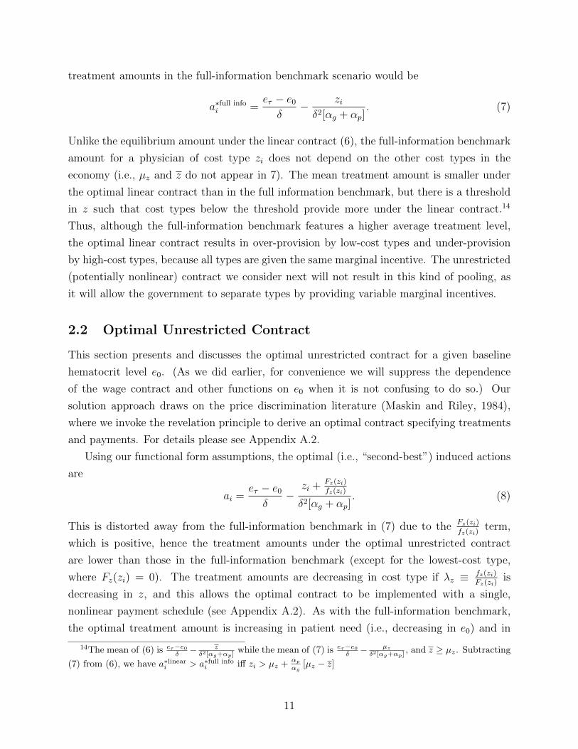
Using our functional form assumptions, the optimal (i.e., “second-best”) induced actions

are

ai =eτ − e0δ

−zi + Fz(zi)

fz(zi)

δ2[αg + αp]. (8)

This is distorted away from the full-information benchmark in (7) due to the Fz(zi)fz(zi)

term,

which is positive, hence the treatment amounts under the optimal unrestricted contract

are lower than those in the full-information benchmark (except for the lowest-cost type,

where Fz(zi) = 0). The treatment amounts are decreasing in cost type if λz ≡ fz(zi)Fz(zi)

is

decreasing in z, and this allows the optimal contract to be implemented with a single,

nonlinear payment schedule (see Appendix A.2). As with the full-information benchmark,

the optimal treatment amount is increasing in patient need (i.e., decreasing in e0) and in

14The mean of (6) is eτ−e0δ − z

δ2[αg+αp]while the mean of (7) is eτ−e0

δ − µzδ2[αg+αp]

, and z ≥ µz. Subtracting

(7) from (6), we have a∗lineari > a∗full infoi iff zi > µz +αpαg

[µz − z]

11

government and physician valuations of patient health, and is decreasing in the physician’s

cost of treatment. Additionally, we note that higher degrees of physician altruism can

blunt the distortion away from the first-best that is caused by the unobserved heterogeneity.

This highlights the potential importance of allowing for both physician heterogeneity and

physician altruism when characterizing optimal payment contracts.

The payments in the unrestricted contract can be derived from the optimal treatment

amounts and the specification of physician utility (see Appendix A.2). The result is

w(ai) =

[∫ z

zi+1

ajdj

]− [αph(ai)− aizi]. (9)

This expression involves the integral of actions by higher cost types (zi+i to z) because the

additive separability in our utility specification allows the IC constraints to simplify in a

way that yields this integral as the utility of cost type zi in equilibrium (see Appendix A.3).

Notably, as in Ellis and McGuire (1986), the payments in the optimal unrestricted contract

result in partial cost sharing if αp > 0; i.e., if physicians are partially altruistic.15

Figure 1 plots outcomes for full-information benchmark (black, solid line), linear con-

tract (red, dotted line), and unrestricted contract (blue, dashed line) scenarios for a specific

parameterization of the model, where physician cost types are distributed according to a

truncated normal distribution. Figure 1a shows the induced action (treatment amount) for

each cost type in each scenario. Under full information (the “first-best”), the treatment

amount decreases as the cost factor z increases. The same is also true in both asymmetric

information scenarios. However the linear contract, which offers the same marginal incen-

tive to all types, leads to over-provision for low-cost types and under-provision for high-cost

types. In contrast, the unrestricted contract, which separates types by providing variable

marginal incentives, leads to under-provision for all but the lowest-cost type, z. The amount

of this distortion relative to the full-information benchmark is increasing in cost type.

Figure 1b shows how the payment depends on the treatment amount under the linear

and unrestricted contracts; in other words, this figure plots the payment schedules. Both

schedules are upward-sloping, meaning that pure prospective payment is not optimal in this

example, similar to Ellis and McGuire (1986). Also similar to Ellis and McGuire (1986),

neither contract implements full cost sharing. The range of payments under the unrestricted

contract is lower than the range under the linear contract, because the nonlinear schedule pro-

vides lower marginal rates and induces lower treatment amounts among low-cost physicians,

and because it induces substantially lower treatment amounts among high-cost physicians

as well. (However, as seen in figure 1a, the unrestricted contract induces higher treatment

15This is because ∂w(ai)∂ai

= zi − αph′(ai), which is strictly less than the marginal cost zi for e0 < eτ .

12

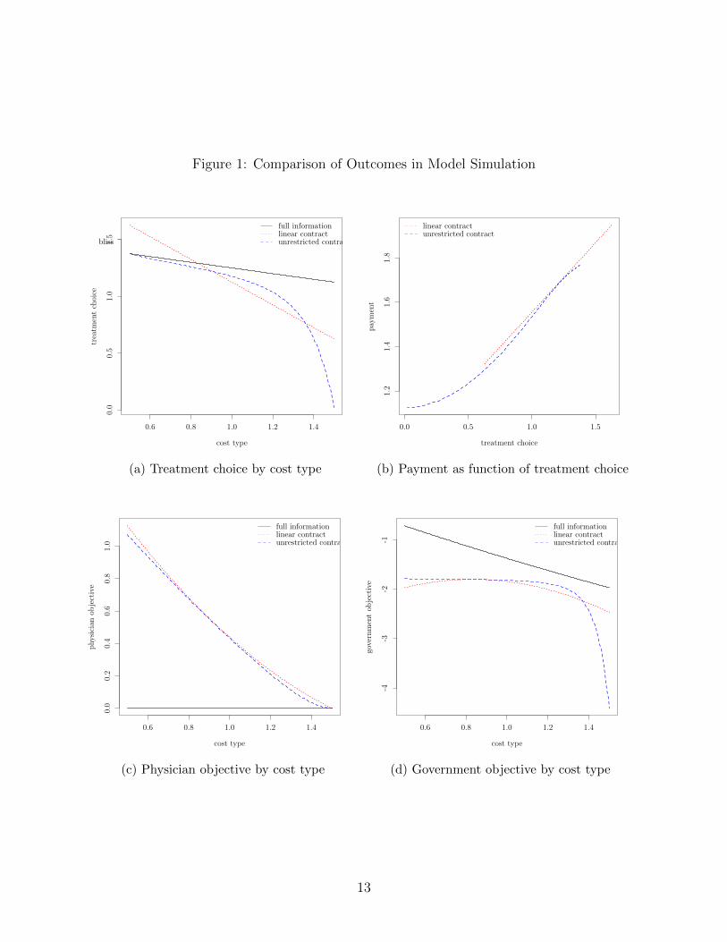
Figure 1: Comparison of Outcomes in Model Simulation

0.6 0.8 1.0 1.2 1.4

0.0

0.5

1.0

1.5

cost type

trea

tmen

tch

oice

bliss

full informationlinear contractunrestricted contract

(a) Treatment choice by cost type

0.0 0.5 1.0 1.5

1.2

1.4

1.6

1.8

treatment choice

pay

men

t

linear contractunrestricted contract

(b) Payment as function of treatment choice

0.6 0.8 1.0 1.2 1.4

0.0

0.2

0.4

0.6

0.8

1.0

cost type

physi

cian

obje

ctiv

e

full informationlinear contractunrestricted contract

(c) Physician objective by cost type

0.6 0.8 1.0 1.2 1.4

-4-3

-2-1

cost type

gove

rnm

ent

obje

ctiv

e

full informationlinear contractunrestricted contract

(d) Government objective by cost type

13

amounts among cost types in the middle of the range.)

The qualitative relationship between payment and treatment amounts depends on the

asymmetric information. In a full-information scenario, the government could fully compen-

sate high-cost types to implement the desired action, thereby paying them more than low-

cost types and leading to a negative relationship between payment and treatment amounts.16

However, the asymmetric information would then enable low-cost types to obtain large sur-

pluses by pretending to be high-cost types. Thus, incentive compatibility requires that

payment and treatment amounts must both be lower for high-cost types, so that low-cost

types enjoy a larger surplus (i.e., are paid more) by providing larger amounts. This results

in a payment contract that increases with treatment amounts.

Finally, figures 1c and 1d respectively plot the physician objective (up) and the govern-

ment objective (ug) against the cost type, in each scenario. Since the government can extract

all the surplus under full information, all cost types receive zero utility in the benchmark

scenario. In the optimal contracts under asymmetric information, only the highest cost type

receives zero utility (because the VP constraint only binds for this type) while all lower cost

types receive positive surpluses. The physician surpluses are in fact quite similar under the

linear and nonlinear contracts in this example. The government naturally fares best under

full information and second-best with the unrestricted contract.17

3 Data

Our data come primarily from Medicare outpatient claims from renal dialysis centers (free-

standing or hospital-based) in 2008 and 2009, for the treatment of patients with ESRD. As

noted earlier, these facilities provide dialysis treatment to patients multiple times per week,

and claims are typically filed monthly. EPO can be administered at each visit, and each

injection is individually listed as a separate line on the claim.

The raw 20% sample for 2008 and 2009 contains 1.4 million ESRD claims with 11.1

million claim lines for EPO or related medications.18 Almost 90% of the claims bill for at

least one injection of these drugs (1.25 million claims). All claims with an injection include

a baseline hematocrit level from the previous month (or a related hemoglobin level), but

16This can be seen by implicitly differentiating the binding participation constraint, resulting in∂w∗full info

i

∂a∗full infoi

= −[zi − αph′(a∗full infoi )

], where we know the term in the brackets is weakly positive because

the full-information treatment choice solves [αg + αp]h′(a∗full infoi ) = zi, and αg ≥ 0.

17The substantial downward distortion of the treatment amounts from high-cost physicians results in lowervalues of the government’s objective from these types, but this is in the far upper tail of the distribution.

18Epoetin alpha constitutes 97.6% of the claim lines for this class of medication in our sample. Thealternative drug was darbepoetin alpha. For the present analysis we restrict to epoetin alpha becausedosages and reimbursements differ between the two drugs.

14

claims without an injection typically do not report a red blood cell level. As a consequence,

for the present analysis we exclude claims without any injections of EPO.

The unit of analysis is the (typically) monthly claim, which reports the treatment given by

provider i to patient j in period t.19 The total amount of EPO injected over the month is the

action, aijt, and the prior hematocrit level reported in the claim is the baseline hematocrit,

e0,jt.20 The reimbursement rate, w1t, is the national payment rate per 1,000 units of EPO

for the quarter in which the claim was filed. These rates are listed in Medicare Part B

Average Sales Price Drug Pricing Files available on the CMS website.21 The claims also

list the actual payments for each injection of EPO, so a claim-specific reimbursement rate

can be computed. These actual reimbursement rates are highly correlated with the national

payment rates.22

In order to avoid extreme outliers, which often reflect data entry errors, we remove

observations where the baseline hematocrit (e0,jt) is above its 99th percentile or below its 1st

percentile or where the amount of EPO (aijt) is above its 99th percentile. The final analytic

sample has 1.1 million claims for 76,985 unique patients from 5,150 unique providers. The

providers are defined as facilities, not individual physicians, because within each facility there

are multiple doctors and nurses who jointly treat their patients.23

Table 1 provides summary statistics on the three main variables in our analytic sample.

The average monthly dosage of EPO is 67.0 thousand units, with a relatively large standard

deviation of 66.4 thousand units, and the average baseline hematocrit is 34.5 percent (volume

percentage of red blood cells in the blood). The national reimbursement rate has a mean

of $9.26 per 1,000 units of EPO and ranges from a low of $8.96 in 2008Q1 to a high of

$9.62 in 2009Q3. Table 1 also presents information on the distribution of acquisition costs

for EPO from a separate source, the Renal Dialysis Facility Cost Reports. The Centers

for Medicare and Medicaid Services (CMS) requires dialysis facilities to submit detailed

annual cost reports, which include their total expenditures on EPO and the total number

of units provided. These data are publicly available on the CMS website.24 From the total

expenditures (less any rebates) and total units, we compute the average acquisition cost per

1,000 units for each facility in the cost report data for 2008. The percentiles listed in the

19Note that we now use i to index providers instead of unobserved types.20For claims that report hemoglobin rather than hematocrit, we use the standard rule of thumb of mul-

tiplying by three to convert the levels.21See https://www.cms.gov/Medicare/Medicare-Fee-for-Service-Part-B-Drugs/

McrPartBDrugAvgSalesPrice/index.html.22In our analytic sample the correlation is 0.92, net of provider fixed effects.23Also, many facilities belong to large, national chains (DaVita and Fresenius), but we treat the individual

facilities separately.24https://www.cms.gov/Research-Statistics-Data-and-Systems/Downloadable-Public-Use-Files/

Cost-Reports/RenalFacility.html

15

Table 1: Summary Statistics

PercentilesVariable Mean SD 10th 25th 50th 75th 90th

Monthly EPO dosage (1,000u) 67.0 66.4 8.8 20.0 45.0 90.0 156.2

Prior hematocrit level (%) 34.5 3.4 30 32.4 34.8 36.9 38.7

Reimbursement rate ($/1000u) 9.26 0.24

Addendum 1 – Percentiles of EPO acquisition costs from annual cost reports:Acquisition cost ($/1000u) 7.13 7.23 7.53 8.15 9.11

Addendum 2 – Medicare reimbursement rate for EPO in each quarter:Reimb. rate ($/1000u) 8.96 9.07 9.07 9.10 9.20 9.40 9.62 9.58

(2008Q1) (Q2) (Q3) (Q4) (2009Q1) (Q2) (Q3) (Q4)

Notes: The EPO dosage and hematocrit come from Medicare outpatient claims data. The reimbursementrate comes from quarterly Medicare Part B ASP Drug Pricing Files for 2008 and 2009. This latter variabletakes one of eight values depending on the quarter, as listed in Addendum 2, so we do not present itspercentiles. The distribution of EPO acquisition costs shown in Addendum 1 is computed from RenalDialysis Facilities Cost Report Data for 2008. We do not present the mean or standard deviation becauseextreme outliers in the cost report data make those statistics unreliable, compared to the percentiles.

table show non-trivial differences across providers in the acquisition cost, even though the

drug was produced by a single manufacturer.

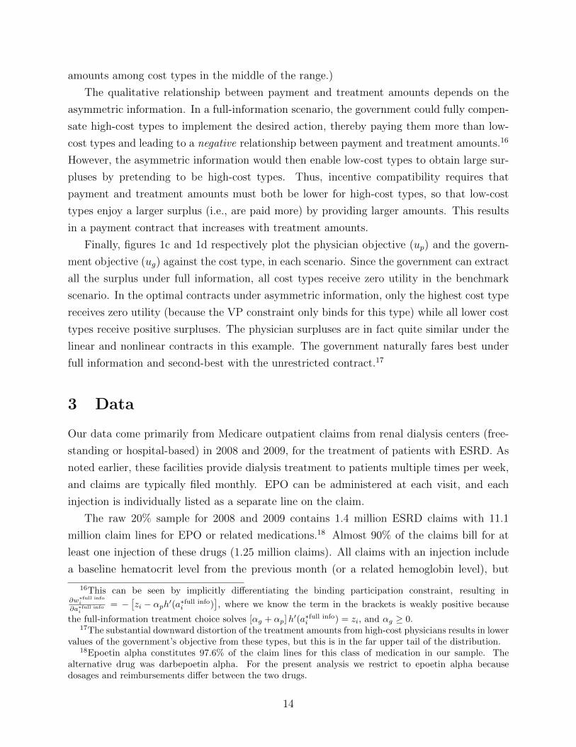
To present some preliminary evidence on the relationships between patient need, payment

rates, and drug provision, Figure 2 plots average dosages of EPO as a function of baseline

hematocrit in the first and last quarters of our analytic sample. In both periods the dosages

decline with higher hematocrit levels, as would be expected, and the decline is steeper at

lower levels. A notable difference between the two periods is that in 2009Q4, when the

reimbursement rate was higher, average dosages are higher for patients with low hematocrit

levels, and these dosages decrease more rapidly in relation to hematocrit. Our empirical

model, discussed next, will use specifications designed to fit these qualitative features.

4 Empirical Implementation

We now describe how we adapt the model from Section 2 to our empirical context. The

model naturally extends to an environment with many agents, each treating many patients,

16

Figure 2: Mean Monthly Dosages of EPO in Relation to Baseline Level of Hematocrit

under the assumptions that the providers’ utility functions and the government’s objective

function are additive across patients.25

The empirical specification extends the example in Section 2.1 by adding flexibility in

relation to the patient’s baseline hematocrit. We add δ(e0) to the parameter δ, which allows

the productivity of EPO to depend on the baseline level of hematocrit.26 Also we add α(e0)

to the altruism parameter, so that the total weight on the patient’s health in the physician’s

utility is αp + α(e0). This means that physicians may have greater or lesser concern for

the health of patients with different baseline levels of hematocrit.27 The physician’s utility

function is thus

− [αp + α(e0)]1

2[[δ + δ(e0)]a+ e0 − eτ ]2 − azi + w0 + w1a.

The parameters α(e0) and δ(e0) are specified take different values over certain intervals of

e0, noted below, which makes this a piecewise quadratic function of a and e0.

25The static framework can be applied to to multiple time periods if there are no dynamic effects of EPO(as discussed in Section 1.2), and if the government does not use treatment histories in setting reimbursementrates. This has always been the case when patient hematocrit levels are within the recommended range.However, the Medicare payment policy during our analysis period paid reduced rates for EPO given topatients who had high hematocrit levels for three consecutive months (over 39%).

26This captures diminishing returns in a simple fashion that maintains our closed-form solutions.27We still refer to physicians when discussing the model, but to be clear, we use facilities as the providers

in the empirical analysis.

17

Given this utility function, the optimal treatment amount (at an interior solution) is

a∗i =[eτ − e0]δ + δ(e0)

+w1 − zi

[αp + α(e0)][δ + δ(e0)]2. (10)

The treatment policy function is thus piecewise linear, with the segments corresponding to

the intervals in e0. As we will show, this specification has the advantages of maintaining

closed-form solutions from Section 2.1 while having sufficient flexibility to fit the qualitative

features seen in Figure 2.

To allow for unexplained variation from the econometrician’s perspective we add an

independent, mean-zero shock η. We also decompose the individual cost type as zi = µz +ζi.

The observed treatment amount provided by physician i to patient j at time t is then

aijt =[eτ − e0jt]δ + δ(e0jt)

+w1t − [µz + ζi]

[αp + α(e0jt)][δ + δ(e0jt)]2+ ηijt, (11)

where e0jt is patient j’s baseline hematocrit in period t and w1t is the national reimburse-

ment rate for EPO in period t. Within each interval of baseline hematocrit, in which the

parameters α(e0) and δ(e0) are constant, (11) is linear in e0 and w1.

4.1 Identification

To derive an optimal contract and simulate provider behavior, we need values for the fol-

lowing structural parameters: αp and α(e0) (altruism weights), δ and δ(e0) (productivity

of EPO), and eτ (target hematocrit level). We also need the distribution of z, because the

mean and maximum (µz and z) appear in the optimal linear contract and the inverse haz-

ard ratio (Fz(z)/fz(z)) appears in the optimal unrestricted contract. These parameters and

the distribution of z can be identified from the reduced form (11), except that we require

additional data on costs to establish the mean value of z (described below).

The reduced form can be re-expressed as follows:

aijt =∑k

1{e0jt ∈ Ek}[βk0 + βk1e0jt + βk2w1t

]+ νi + εijt, (12)

where 1{e0jt ∈ Ek} indicates that the baseline hematocrit is in interval Ek. This is a

piecewise linear regression model with provider fixed effects. The parameters δ+ δ(Ek) and

αp + α(Ek) are recovered from the coefficients of this regression as follows:

δ + δ(Ek) = − 1

βk1and αp + α(Ek) =

[βk1 ]2

βk2,

18

with the δ(Ek) and α(Ek) in one interval normalized to zero.28 The result for the altruism

parameters has intuitive appeal: it is the ratio of the responsiveness to a measure of patient

need (squared) to the responsiveness to remuneration. The intercept in each interval, βk0 ,

identifies a linear combination of eτ and µz, and the distribution of the provider fixed effects

identifies the distribution of deviations from the mean cost. We use external data, from the

Renal Dialysis Facility Cost Reports, to identify the mean per-unit cost, µz. Specifically we

take the median value reported in Table 1 as the value of µz, which is equal to $7.53 per

1,000 units.29 This then completes the identification of the distribution of z (from the fixed

effects) and the target level of hematocrit eτ (from the intercepts).

The identification of the structural parameters also depends on the consistency of the

reduced-form coefficient estimates. There are two variables in the reduced form (12): the

baseline hematocrit (e0jt) and the national payment rate (w1t). These must be uncorrelated

with the error term (εijt) net of the provider fixed effects (νi). The baseline hematocrit

satisfies this so long as any selection of patients to providers did not change over the two

years of our estimation period. That makes the within-provider variation in e0jt across

patients and over time exogenous.30 The national payment rate, as described in Section

1.2, was determined by the national average price of EPO roughly six months earlier. An

individual facility could not affect the national average price, but if demand shocks were

substantially correlated across facilities and over time, there could be a bias. However we

include a year dummy for 2009 and month dummies for each calendar month. These would

address both secular and cyclical trends in demand. Also, dialysis facilities were not the

only purchasers of EPO because the drug was also widely used in chemotherapy. Thus there

are two potential sources of exogenous variation in the lagged prices that determined w1t:

demand shocks from chemotherapy providers and supply shocks from the drug manufacturer.

28The coefficients of the reduced form are the following combinations of the structural parameters:

βk0 = eτδ+δ(Ek)

− µz[αp+α(Ek)][δ+δ(Ek)]2

βk1 = − 1δ+δ(Ek)

βk2 = 1[αp+α(Ek)][δ+δ(Ek)]2

.

29We use the median rather than the mean because it is less sensitive to extreme outliers in the costreport data. Also to be precise, the cost reports reflect the acquisition cost but not any additional cost ofadministering the drug. The cost of injecting EPO is nevertheless small relative to the price of purchasingit.

30A more subtle concern is the fact that the hematocrit level from the prior month reflects the treatmentgiven in the prior month. So long as each provider’s treatment protocols are stable during our analysisperiod, the provider fixed effects would address this as well.

19

Table 2: Reduced-Form Coefficient Estimates

Interval of Baseline HematocritCoefficient Up to 27, > 27 to 30, > 30 to 33, > 33 to 36, > 36 to 39, > 39

βk0 352.1 173.7 281.1 229.3 153.8 28.3Constant term (46.0) (51.3) (28.2) (18.7) (17.9) (25.1)

βk1 -6.20 -7.56 -9.48 -6.70 -4.00 -2.06Baseline HCT (0.14) (0.37) (0.20) (0.13) (0.13) (0.16)

βk2 -7.20 17.09 11.45 7.22 4.97 10.40Reimb. rate (5.21) (5.64) (3.10) (2.03) (1.94) (2.76)

Obs. in interval 97,983 82,640 216,391 379,530 267,245 83,344

Notes: Estimates are from a single fixed-effects regression where variables are interacted with indicators forthe listed ranges in baseline hematocrit (HCT). Standard errors in parentheses, clustered by provider.

4.2 Estimation

We estimate (12) via standard fixed effects estimation with provider fixed effects. As noted

above, the regression also includes separate effects for year and month (not year x month).

The year effect(s) capture possible secular changes, while the month effects account for billing

behavior that may change throughout the year (e.g., a spike in claims dated December 31).

Table 2 presents the estimates of the main coefficients. These come from a single regression

with separate coefficients for each of the listed intervals of baseline hematocrit. For example,

in the interval from 30 to 33, a patient with one unit higher hematocrit (say 32 vs. 31)

receives 9,480 less units of EPO per month on average. Also for patients in the interval from

30 to 33, a one dollar increase in the reimbursement rate (per 1,000 units) would induce

providers to increase dosages by 11,450 units per month on average.

The intervals of baseline hematocrit were chosen to reflect treatment guidelines and

policies in place at the time, and to balance the flexibility of the specification with the

precision of the estimates for each interval. The FDA approved EPO for use in patients

with hematocrit between 30 and 36, and Medicare reduced the reimbursement rate for EPO

provided to patients with hematocrit above 39.31 Using 3-point intervals divides this range

from 30 to 39 evenly, and the estimation results indicate that this width allows sufficient

power within each interval while maintaining flexibility globally. We consider the estimates

in the intervals from 30 up to 39 to be the most reliable, because these are the most common

31Medicare did not use 36% as the cutoff for payment reductions because of the acknowledged difficultyin maintaining a target level exactly over time.

20

Table 3: Structural Parameter Estimates

Interval of Baseline HematocritParameter Up to 27, > 27 to 30, > 30 to 33, > 33 to 36, > 36 to 39, > 39

Providers’ value of health in dollarsαp + α(Ek) -5.34 3.34 7.84 6.22 3.22 0.41

(3.89) (1.15) (2.15) (1.77) (1.28) (0.12)

Increase in HCT from 1000u EPOδ + δ(Ek) 0.161 0.132 0.105 0.149 0.250 0.486

(0.004) (0.007) (0.002) (0.003) (0.008) (0.037)

Implied HCT target using µz = $7.53eτ 48.0 40.0 38.8 42.3 47.8 51.9

(1.3) (1.2) (0.5) (0.4) (0.7) (2.1)

Notes: Values are recovered from reduced form coefficients, using the value of µz = $7.53, as described inSection 4.1. Delta method standard errors in parentheses.

clinically (over 80% of the observations are in these intervals) and because this range has

at least implicit approval from the FDA or Medicare policy. Within this range there is

decreasing responsiveness to both baseline hematocrit and the reimbursement rate, going

from lower to higher intervals. This matches the decreasing magnitude of the slopes seen in

Figure 2.

Table 3 presents the structural parameters, recovered as described above. Across the

intervals from 30 to 39, the altruism weight decreases while the productivity of EPO increases.

The former could be interpreted as a lower concern for the health of patients with less severe

anemia. The latter is consistent with diminishing marginal productivity of EPO.32 The

magnitudes of the altruism parameters imply that, for example in the interval from 30 to

33, physicians would require $7.84 to compensate for providing an amount of EPO intended

to achieve a hematocrit above or below the target level by 1 percentage point. The estimate

of δ + δ(Ek) in this interval implies that 1,000 units of EPO raises hematocrit by 0.105

percentage points. This and the other estimates of the average productivity of EPO across

the intervals from 30 to 39 are consistent with estimates obtained from clinical trials.33 The

32Patients with lower baseline hematocrit are given more EPO on average, and the estimates of δ+ δ(Ek)reflect the average productivity of EPO for patients with baseline hematocrit in each range.

33The average dosages and the average increases from initial hemoglobin levels reported in Singh et al.(2006) imply average productivities of 0.143 and 0.167 for the two treatment groups in the study (ourcalculations). Also, Tonelli et al. (2003) construct a dose-response curve based on results from five otherclinical trials, which indicates average marginal productivities ranging from 0.135 to 0.241 for hematocritlevels in this range.

21

values of the implied hematocrit target are also reasonably close to what would be expected

based on clinical and policy guidelines.34

5 Quantitative Results

We now present preliminary results on the optimal linear contract and optimal unconstrained

contract. First we compute the optimal per-unit payment rate in the linear contract (wlin1 )

and use it to simulate counterfactual EPO dosages for the entire sample. We then construct

the optimal unrestricted contract for a particular value of baseline hematocrit, and compare

this with the linear contract and the observed contract (i.e., the actual reimbursement rate).

The reimbursement rate in the optimal linear contract depends on mean and maximum

costs (µz and z) and the altruism weights for both the providers and the government (αp and

αg).35 However, the altruism weight for the government cannot be recovered without making

further assumptions (e.g., that the observed payment policy is optimal, an assumption we

do not want to make). Instead we consider two possible values for αg that span a wide

range. Specifically, we use αg = αp as the low value and αg = 10αp as the high value. Also,

because the maximum cost z is highly sensitive to outliers, we use the 95th percentile of the

recovered distribution of z in place of the maximum. We then use the estimated reduced

form to predict a counterfactual dosage for each observation (i.e., for each patient in each

month).36

Table 4 shows the results of this exercise. The actual reimbursement rates range from

$8.96 to $9.62 (over time), and with these observed rates the average predicted monthly

dosages for patients within each interval of baseline hematocrit essentially match the aver-

age observed dosages (by construction). The payment rate in optimal linear contract with

αg = 10αp is $6.44, and with αg = αp is $1.54.37 With the higher counterfactual rate,

dosages are reduced by about 30–40% and with the lower rate they are reduced even further.

Interestingly, with the $6.44 rate the proportional reductions are largest in the top interval

of baseline hematocrit, where Medicare sought to discourage the use of EPO.

Figure 3 presents our results for the optimal unrestricted contract. The contract is com-

puted for the median level of baseline hematocrit (e0 = 34.8) and with the high value for

34These implied targets are slightly higher than one would expect based on the FDA and Medicare policies(e.g., 36 or 39). This indicates a misspecification in the model, for example in the quadratic loss around thetarget, but the misspecification is mild because the implied targets are rather close to the expected amounts.

35See equation (5).36Negative predicted dosages are replaced with 0.37Although αp varies across the intervals of baseline hematocrit, the reimbursement rate does not vary

because we have set αg to be proportional to αp, which makes these parameters cancel in equation (5).

22

Figure 3: Optimal Contracts and Treatment Choices

20 40 60 80

300

400

500

600

700

800

900

treatment choice

pay

men

t

observed contractlinear contractunrestricted contract

(a) Payment as function of treatment amount

4 6 8 10 12

2040

6080

cost typetr

eatm

ent

choi

ce

observed contractfull informationlinear contractunrestricted contract

(b) Treatment choice by cost type

20 40 60 80

0.00

0.05

0.10

0.15

treatment choice

den

sity

observed contractlinear contractunrestricted contract

(c) Distribution of treatment amounts

4 6 8 10 12

0.04

0.06

0.08

0.10

0.12

0.14

0.16

cost type

den

sity

(d) Distribution of cost types

Notes: Panel (a) shows the payment contract (i.e., total payment as a function of the treatment amount) forthe observed contract and the optimal linear and unrestricted contracts derived from the estimated model.Panel (b) shows the treatment amounts chosen under these contracts as a function of the physician costtype. The observed contract uses the sample mean of the payment rate ($9.26). The optimal contracts arecomputed from the estimated parameters and the recovered distribution of cost types, using equations (3)and (5) for the linear contract and equations (8) and (9) for the unrestricted contract. The contracts andoutcomes are computed for a patient with the median level of baseline hematocrit (34.8).

23

Table 4: Simulation of Average Monthly Dosages of EPO under Linear Contracts

Scenario Interval of Baseline Hematocrit($ rate) Up to 27, > 27 to 30, > 30 to 33, > 33 to 36, > 36 to 39, > 39

Observed reimbursement rates($8.96–$9.62) 79.6 114.2 85.5 62.1 48.6 39.7

Optimal linear contract, αg = 10αp($6.44) 99.8 65.9 53.2 42.0 35.0 13.8

Optimal linear contract, αg = αp($1.54) 135.0 2.4 6.7 11.4 13.6 0.2

Notes: Predicted monthly dosages are generated for each observation in the sample using the estimatedversion of (12), with the payment rate set to the observed amounts, or $6.44, or $1.54, as indicated.

government altruism (αg = 10αp).38 The payment and treatment amounts are shown for the

observed contract (green, long-dashed line), the optimal linear contract (red, dotted line),

and the optimal unrestricted contract (blue, dashed line). Figure 3a plots the contracts; i.e.,

how the total payment depends on the treatment amount. Figure 3c underneath shows the

distribution of treatment amounts provided under each contract (to patients with e0 = 34.8).

Consistent with the payment rates presented in Table 4, the observed contract is steeper (i.e.,

has a higher per-unit rate) than the optimal linear contract, even though the government

values patient health ten times as much as do physicians. The optimal unrestricted contract

has a roughly similar average payment rate as the optimal linear contract, but the govern-

ment’s ability to provide different marginal incentives for different dosages results in a much

more compressed distribution of treatment amounts under this contract.

Figure 3b shows how treatment amounts are related to physician cost types under each

contract. The full-information benchmark is included for comparison (gray, solid line). Con-

sistent with Table 4, treatment amounts under the observed contract are too high, exceeding

first-best, full-information dosages and even the implied bliss point (i.e., eτ ) for most cost

types. The optimal linear contract offers a uniformly lower payment rate, so dosages under

this contract lie below those under the observed contract, and the two move in parallel. The

optimal unrestricted contract, which better separates physician types, is much closer to the

full-information benchmark. In contrast to both the observed and optimal linear contracts,

the optimal unrestricted contract leads to mild under-provision for most cost types. This

indicates the potential importance of the subtle differences between the optimal linear and

38We trim the distribution of cost types at the 5th and 95th percentiles and use this as the Fz. For theobserved contract we use the sample mean of the actual reimbursement rates, $9.26.

24

Table 5: Summary of Outcomes under Optimal Contracts

Contract Mean Pmt Mean Dosage SD DosageObserved $582 62.9 12.5Linear $440 42.3 12.5Unrestricted $484 42.4 13.7Full Information $342 45.4 11.1

Note: Table shows summary statistics of outcomes plotted in Figure 3.

unrestricted contracts seen in Figure 3a.

Table 5 summarizes the outcomes under these contracts (again, for patients with the

median level of hematocrit). With the observed contract, the predicted mean payment

is $582 and the predicted mean dosage is 62,900 units of EPO per month. The optimal

linear contract reduces the mean payment by 25% and the mean dosage by 33%.39 The

optimal linear contract does not change the variation in dosages, however, because it provides

a constant marginal incentive just like the observed contract. The optimal unrestricted

contract, by contrast, is nonlinear and induces a substantial reduction in the variation in

treatment amounts across physicians. The standard deviation of the dosages falls by 70%,

while the mean dosage is essentially the same as with the optimal linear contract. The mean

payment is larger under the nonlinear contract compared to the linear contract, but this

relatively small additional expenditure yields better patient health because of the reduction

in treatment variation. Finally, for comparison, the full information scenario indicates what

could be obtained in the absence of asymmetric information about physician costs. The

mean dosage is slightly higher than under the optimal contracts, while the mean payment

is lower (because all physicians receive zero surplus). Some variation in treatment amounts

remains, which reflects the government’s valuation of the physicians’ actual marginal costs.

39The optimal linear contract also includes a fixed payment, w0, here equal to $168.

25

References

Abito, J. M., “Welfare Gains From Optimal Pollution Regulation,” Working Paper, 2017.

Chalkley, M. and J. M. Malcomson, “Contracting for Health Services when Patient Demand

does not Reflect Quality,” Journal of Health Economics, 17(1):1 – 19, 1998, ISSN 0167-

6296, doi: https://doi.org/10.1016/S0167-6296(97)00019-2.

—, “Government Purchasing of Health Services,” in A. J. Culyer and J. P. Newhouse, eds.,

“Handbook of Health Economics,” vol. 1 of Handbook of Health Economics, pp. 847 – 890,

Elsevier, 2000, doi: https://doi.org/10.1016/S1574-0064(00)80174-2.

Chandra, A., D. Cutler and Z. Song, “Who Ordered That? The Economics of Treatment

Choices in Medical Care,” Handbook of Health Economics, 2:397–432, 2012.

Chiappori, P.-A., B. Jullien, B. Salanie and F. Salanie, “Asymmetric Information in In-

surance: General Testable Implications,” RAND Journal of Economics, 37(4):783–798,

2006.

Chiappori, P.-A. and B. Salanie, “Testing Contract Theory: A Survey of Some Recent

Work,” in M. Dewatripont, L. P. Hansen and S. Turnovky, eds., “Advances in Economics

and Econometrics: Eighth World Congress,” vol. 1, pp. 115–149, Cambridge University

Press, 2003.

Chone, P. and C.-t. A. Ma, “Optimal Health Care Contract Under Physician Agency,”

Annals of Economics and Statistics/Annales d’Economie et de Statistique, pp. 229–256,

2011.

Clemens, J. and J. D. Gottlieb, “Do Physicians’ Financial Incentives Affect Medical Treat-

ment and Patient Health?” American Economic Review, 104(4):1320–49, 2014, doi:

10.1257/aer.104.4.1320.

De Fraja, G., “Contracts for Health Care and Asymmetric Information,” Journal of Health

Economics, 19(5):663–677, 2000.

Deneckere, R. and S. Severinov, “Multi-dimensional Screening: A Solution to a Class of

Problems,” Tech. rep., mimeo, econ. ucsb. edu, 2015.

Einav, L., A. Finkelstein and J. Levin, “Beyond Testing: Empirical Models of Insurance

Markets,” Annual Review of Economics, 2(1):311–336, 2010.

26

Elliott, S., E. Pham and I. C. Macdougall, “Erythropoietins: A Common Mechanism of

Action,” Experimental Hematology, 36(12):1573–1584, 2008.

Ellis, R. P. and T. G. McGuire, “Provider Behavior under Prospective Reimbursement: Cost

Sharing and Supply,” Journal of Health Economics, 5(2):129–151, 1986.

Gagnepain, P. and M. Ivaldi, “Incentive Regulatory Policies: The Case of Public Transit

Systems in France,” RAND Journal of Economics, pp. 605–629, 2002.

GAO, “End-Stage Renal Disease: Bundling Medicare’s Payment for Drugs with Payment

for All ESRD Services Would Promote Efficiency and Clinical Flexibility,” Tech. Rep.

GAO-07-77, U.S. Government Accountability Office, Washington, DC, 2006.

Gayle, G.-L. and R. A. Miller, “Has Moral Hazard Become a More Important Factor in

Managerial Compensation?” American Economic Review, 99(5):1740–1769, 2009.

Gaynor, M. and M. Pauly, “Compensation and Productive Efficiency in Partnerships: Evi-

dence From Medical Groups Practice,” Journal of Political Economy, pp. 544–573, 1990.

Gaynor, M., J. Rebitzer and L. Taylor, “Physician Incentives in Health Maintenance Orga-

nizations,” Journal of Political Economy, pp. 915–931, 2004.

Godager, G. and D. Wiesen, “Profit Or Patients’ Health Benefit? Exploring The Hetero-

geneity In Physician Altruism,” Journal of Health Economics, 32(6):1105–1116, 2013.

Jack, W., “Purchasing Health Care Services From Providers With Unknown Altruism,”

Journal of Health Economics, 24(1):73–93, 2005.

Jacques, L. B., T. S. Jensen, J. Rollins, K. Long and E. Koller, “Final Decision Memorandum

for CAG # 00413N: Erythropoiesis Stimulating Agents (ESA) for Treatment of Anemia in

Adults with CKD Including Patients on Dialysis and Patients not on Dialysis,” Tech. Rep.

CAG # 00413N, Centers for Medicare and Medicaid Services, Washington, DC, 2011.

Malcomson, J. M., “Supplier Discretion Over Provision: Theory and an Application to

Medical Care,” RAND Journal of Economics, 36(2):412–432, 2005.

Maskin, E., J. J. Laffont, J. Rochet, T. Groves, R. Radner and S. Reiter, Optimal Nonlin-

ear Pricing with Two-Dimensional Characteristics, pp. 256–266, University of Minnesota

Press, Minneapolis, 1987.

Maskin, E. and J. Riley, “Monopoly with Incomplete Information,” RAND Journal of Eco-

nomics, 15(2):171–196, 1984.

27

McGuire, T. G., “Physician Agency,” Handbook of Health Economics, 1:461–536, 2000.

Paarsch, H. J. and B. Shearer, “Piece Rates, Fixed Wages, and Incentive Effects: Statistical

Evidence from Payroll Records,” International Economic Review, 41(1):59–92, 2000.

Singh, A. K., L. Szczech, K. L. Tang, H. Barnhart, S. Sapp, M. Wolfson and D. Reddan,

“Correction of Anemia with Epoetin Alfa in Chronic Kidney Disease,” New England Jour-

nal of Medicine, 355(20):2085–2098, 2006, doi: 10.1056/NEJMoa065485, pMID: 17108343.

Tonelli, M., W. C. Winkelmayer, K. K. Jindal, j. William F. Owen and B. J. Manns,

“The Cost-effectiveness of Maintaining Higher Hemoglobin Targets with Erythropoietin

in Hemodialysis Patients,” Kidney International, 64:295–304, 2003.

Wilson, R. B., Nonlinear Pricing, Oxford University Press on Demand, 1993.

Wolak, F. A., “An Econometric Analysis of the Asymmetric Information, Regulator-Utility

Interaction,” Annales d’Economie et de Statistique, pp. 13–69, 1994.

28

A Model Details

A.1 Linear Contract with Cost Heterogeneity

The government’s problem in (4) maximizes patient health, net the cost of transfers, subject

to using a linear contract. Note that we can remove all participation constraints except for

that for physician cost type z because up(a, z) is decreasing in z; i.e., the only participation

constraint that binds is that of the highest cost type. Using interior physician’s policy

functions, government’s problem (4) can be rewritten as

max{(w0,w1)∈R2}

∫ z

z

[ug(a)− w0 − w1a(z, w)] f(z)dz (13)

s.t.

uz(a∗(z, w), w) ≥ 0, VP

a∗(z, w) =eτ − e0δ

+w1 − zδ2αp

, ∀z IC.

Setting up the Lagrangian based on this constraint and using interior physician’s policy

functions we obtain

L =

∫ z

z

[αg(−(w1 − z)2

2δ2α2p

)− w0 − w1((eτ − e0)

δ+w1 − zδ2αp

)

]f(z)dz

+ µ

[(w1 − z)2

2δ2α2p

) +(eτ − e0)(w1 − z)

δ+ w0

].

First order conditions with respect to w0 and w1 yield the following system of equations:∫ z

z

[−f(z)dz] + µ = 0⇒ µ = F (z) = 1∫ z

z

[−αg

[w1 − zδ2α2

p

]−[

(eτ − e0)δ

+w1 − zδ2αp

]− w1

δ2αp

]f(z)dz + µ

[w1 − zδ2αp

+eτ − e0δ

]= 0.

The first part of the second equation has to do with the average of the cost type distribution

while the last term of the second equation, following the multiplier µ, pertains to the binding

participation constraint of the highest-cost-type. Using µ = 1, from the first equation, the

29

second equation can be simplified further to

− [αg + αp]w1

δ2α2p

− z

δ2αp+

∫ z

z

[[αg + αp]z

δ2α2p

f(z)dz

]= 0

⇒ w∗1 =

∫ z

z

zf(z)dz − αpz

αp + αg= µz −

αpαp + αg

z

The next step is to characterize w∗0, which we do using the binding participation constraint

of z:

uz(a∗(z, w), w) =

(w1 − z)2

2δ2αp+

(eτ − e0)(w1 − z)

δ+ w0 = 0

⇒ w∗0 = −w1 − zδ

[(eτ − e0) +

w1 − z2δαp

]Plugging in w∗1 = µz − αp

αp+αgz one can characterize w0 as

w0 =

[2 + αg

αp

]z −

[1 + αg

αp

]µz

δ[1 + αg

αp

]eτ − e0

δ+µz

[1 + αg

αp

]−[2 + αg

αp

]z

2δ [αp + αg]

A.1.1 Comparative Statics

Comparative statics for w∗1 Based on equation (5) it is clear that

∂w∗1∂z

< 0

∂w∗1∂αg

> 0

∂w∗1∂αp

= − µαg(αp + αg)2

< 0.

Comparative statics for w∗0 To do comparative statics for w∗0, we first define the indirect

utility function for a physician of type z, Vp(z;w), which is obtained by plugging the interior

solution of the physician’s action into the utility function. Note that this constraint for the

highest cost type is binding under the optimal linear contract, i.e., they get no surplus. Thus,

Vp(z;w∗0, w∗1) =

(w∗1 − z)2

2δ2αp+

(eτ − e0)(w∗1 − z)

δ+ w∗0 = 0.

30

We use the binding constraint on the indirect utility function for the high cost type for the

comparative static analysis.

∂Vp(z;w∗0, w∗1)

∂z= 0 ⇐⇒ ∂w∗0

∂z− 2

w∗1 − z2δ2αp

+ 2w∗1 − z2δ2αp

∂w∗1∂z− (eτ − e0)

δ+

(eτ − e0)δ

∂w∗1∂z

= 0

⇐⇒ ∂w∗0∂z

= (1− ∂w∗1∂z

)(w∗1 − zδ2αp

+(eτ − e0)

δ) = a∗linearz (1− ∂w∗1

∂z) > 0.

∂Vp(z;w∗0, w∗1)

∂z= 0 ⇐⇒ ∂w∗0

∂αg+ 2

w∗1 − z2δ2αp

∂w∗1∂αg

+(eτ − e0)

δ

∂w∗1∂αg

= 0

⇐⇒ ∂w∗0∂αg

= −∂w∗1

∂αg(w∗1 − zδ2αp

+(eτ − e0)

δ) = −a∗linearz

∂w∗1∂αg

< 0.

∂Vp(z;w∗0, w∗1)

∂z= 0 ⇐⇒ ∂w∗0

∂αg− (w∗1 − z)2

2δ2α2p

+w∗1 − zδ2αp

∂w∗1∂αp

+(eτ − e0)

δ

∂w∗1∂αp

= 0

⇐⇒ ∂w∗0∂αp

=(w∗1 − z)2

2δ2α2p

− ∂w∗1∂αp

(w∗1 − zδ2αp

+(eτ − e0)

δ)

= −h(a∗linearz , e0)−∂w∗1∂αp

a∗linearz > 0.

A.2 Unrestricted Contract with Cost Heterogeneity

We now solve for the optimal unrestricted contract for a given baseline hematocrit level e0.

(As we did earlier, for convenience we will suppress the dependence of the wage schedule

and other functions on e0 when it is not confusing to do so.) This section considers the

specification where types represent cost heterogeneity; Section A.4 considers the specification

where types represent altruism heterogeneity.

First, we show how two useful properties for the agent’s utility function can be obtained

from reasonable assumptions on the primitives. The properties are monotonicity and single-

crossing with regard to the unobserved heterogeneity. They arise from the assumptions on

health production function described earlier and from monotonicity and complementarity

assumptions in the cost function. These assumptions are formally stated below.

Assumption 1. Technology and Costs

We assume the technology and cost functions have the following properties:

31

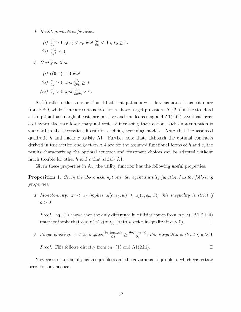
1. Health production function:

(i) ∂h∂a> 0 if e0 < eτ and ∂h

∂a< 0 if e0 ≥ eτ

(ii) ∂2h∂a2

< 0

2. Cost function:

(i) c(0; z) = 0 and

(ii) ∂c∂a> 0 and ∂2c

∂2a≥ 0

(iii) ∂c∂z> 0 and ∂2c

∂z∂a> 0.

A1(1) reflects the aforementioned fact that patients with low hematocrit benefit more

from EPO, while there are serious risks from above-target provision. A1(2.ii) is the standard

assumption that marginal costs are positive and nondecreasing and A1(2.iii) says that lower

cost types also face lower marginal costs of increasing their action; such an assumption is

standard in the theoretical literature studying screening models. Note that the assumed

quadratic h and linear c satisfy A1. Further note that, although the optimal contracts

derived in this section and Section A.4 are for the assumed functional forms of h and c, the

results characterizing the optimal contract and treatment choices can be adapted without

much trouble for other h and c that satisfy A1.

Given these properties in A1, the utility function has the following useful properties.

Proposition 1. Given the above assumptions, the agent’s utility function has the following

properties:

1. Monotonicity: zi < zj implies ui(a; e0, w) ≥ uj(a; e0, w); this inequality is strict if

a > 0

Proof. Eq. (1) shows that the only difference in utilities comes from c(a, z). A1(2.i,iii)

together imply that c(a; zi) ≤ c(a; zj) (with a strict inequality if a > 0).

2. Single crossing: zi < zj implies ∂ui(a;e0,w)∂a

≥ ∂uj(a;e0,w)

∂a; this inequality is strict if a > 0

Proof. This follows directly from eq. (1) and A1(2.iii).

Now we turn to the physician’s problem and the government’s problem, which we restate

here for convenience.

32

Physician’s problem: Given w and e0, physician i chooses a drug treatment level ai to

solve

maxa≥0

ui(a; e0, w).

The solution a∗(z; e0, w) will satisfy

αph′(a∗) + w′(a∗) ≤ c′(a∗; zi).

Government’s problem: The government solves

maxwinW

∫ z

z

[αgh(a, e0)− w(a)] fz(z)dz (14)

s.t.

a = a∗(zi; e0, w), IC

ui(a∗(zi; e0, w); e0, w) ≥ 0,∀i ∈ I VP,

where W is the set of functions containing all possible contracts.

Characterizing the optimal unrestricted wage schedule is complicated, due to the con-

siderable flexibility allowed by W. Therefore, we take the standard approach of considering

the equivalent direct revelation mechanism, in which the government offers a menu of pairs

{(ai, ti)}i∈I , where each (ai, ti) ∈ R+×R, to the physician, who truthfully reveals their type

i.40 In such a mechanism, the physician tells the government their type, after which the

government implements their “prescribed” action ai. We can then determine the optimal

w(ai) by identifying the relevant ti for action ai.41

We show how to arrive at the government’s transformed problem in Appendix A.3, which

allows for a direct solution of treatment levels for a physician of each cost type. For conve-

nience, we reproduce the government’s transformed, or “relaxed”, problem here:

max{ai}i∈I

∫ z

z

[[ug(ai) + up(ai, zi)] fz(zi)− aiF (zi)] dzi. (15)

Note that the relaxed problem drops the monotonicity constraint required to implement the

direct revelation mechanism. As is standard, we proceed by first solving for the set of actions

and then verifying that the actions satisfy monotonicity.

40See the literature on price discrimination, e.g., Maskin and Riley (1984).41For each baseline hematocrit e0, the resulting w(ai) could be thought of as either a menu of linear

schedules, one for each cost type i ∈ I, or a single, potentially nonlinear, schedule. We treat the optimalcontract as the latter, as we find it a more intuitive representation.

33

Solution: By differentiating (15) with respect to the action of cost-type i, we obtain

∂ug(ai)

∂ai+∂up(ai, zi)

∂ai=Fz(zi)

fz(zi),

where Fz(zi)fz(zi)

is the reciprocal of the reverse hazard function, λz(zi); i.e., λz(zi) represents the

likelihood of being cost type zi conditional on not being above that cost type. Because the

right side is strictly positive, the action of ai will be distorted for all but the lowest-cost type;

i.e., we obtain the standard “no distortion at the top” result (where the “top” is the best

type with the lowest cost). If z has the monotone decreasing hazard property, then Fz(zi)fz(zi)

is increasing in i, meaning actions become increasingly distorted as we consider higher and

higher cost types.42

To provide more intuition, we show the optimal treatment choice, using our functional

form assumptions:

ai =eτ − e0δ

−zi + Fz(zi)

fz(zi)

δ2[αg + αp]. (16)

As discussed above, treatment choice will be decreasing in cost type, i.e., the required mono-

tonicity condition (20) will be satisfied, if λz is decreasing in z. Optimal treatment choice

is increasing in need (i.e., decreasing in baseline hematocrit e0) and government and physi-

cian valuation of health, and is decreasing in the cost of treatment. Note that the afore-

mentioned distortions mean that actions characterized in (16) are lower than those in the

full-information benchmark, (7), for all but the lowest-cost type. However, increases in

physician altruism αp can blunt the distortions induced by unobserved heterogeneity. This

highlights the usefulness of allowing for physician heterogeneity and physician altruism when

characterizing optimal remuneration for physicians.

Based on the optimal treatment choice the nonlinear transfer, or wage, function can be

obtained by substituting for surplus

ti = w(ai) = ui − up(ai, zi) =

[∫ z

zi+1

ajdj

]+ aizi − αph(ai),

which, as in Ellis and McGuire (1986), results in partial cost sharing if αp > 0, i.e., physicians

are altruistic.43 Using our functional form assumptions to use (16) to substitute for treatment

42This is analogous to the standard monotone increasing hazard condition, because as we decrease z weencounter “better” cost types.

43This is because ∂w(ai)∂ai

= zi − αph′(ai), which is strictly less than the marginal cost zi for e0 < eτ .

34

choice results in the following expression for the equilibrium transfer

ti =αp2

[zi + Fz(zi)

fz(zi)

δ2[αg + αp]

]2+ aizi +

∫ z

zi+1

eτ − e0δ

−zj +

Fz(zj)

fz(zj)

δ2[αg + αp]

dzj. (17)

We now address indirect implementation, which is relevant for applying the above solution

to the real world using a schedule depending on a, instead of direct implementation via

revelation. Note that ai is strictly monotonic in type. If ti is also strictly monotonic then we

could indirectly implement the direct revelation mechanism via a single nonlinear schedule

t(a), or w(a), since each cost type would have a unique treatment choice and each transfer

would correspond to a unique action and, hence, cost type. Due to the single-crossing

condition, transfer ti increasing in action ai would be equivalent to ti being decreasing in

cost type zi. Differentiating (17), the transfer function will be decreasing in z when44

∂ti∂zi

=∂ai∂zi

[zi − αp

∂h(ai)

∂ai

]< 0

which occurs if [zi − αp

∂h(ai)

∂ai

]> 0 ⇐⇒ Fz(zi)

fz(zi)<αgαpzi.

The left and right sides of the last expression are both increasing in z; therefore, only if αg is

sufficiently high (relative to αp) will the wage increase in action. Intuitively, transfers serve

to compensate physicians for treatment costs. If physicians have a high enough valuation of

patient health, these transfers become less important. As with the optimal linear contract,

to understand how physician altruism affects incentive strength we now examine the slope of

the transfer function is affected by an increase in altruism. Differentiating ∂ti∂zi

with respect

to αp, we find ∂2ti∂zi∂αp

= ∂2ai∂zi∂αp

[zi − αp ∂h(ai)∂ai

]+ ∂ai

∂zi

[− ∂h(ai)

∂ai−αp ∂

2h(ai)

∂a2i

∂ai∂αp

], which is positive

if Fz(zi)fz(zi)

< αgαpzi, i.e., if the condition guaranteeing a monotonic wage function holds. Since

this condition ensures that ∂ti∂zi

< 0, increasing physician altruism dampens the relationship

between physician treatment choices and reimbursement. Intuitively, higher altruism reduces

the importance of cost heterogeneity, the driving force behind the existence of an increasing

wage function.

44See Appendix A.3.1 for details.

35

A.3 Further Details for Unrestricted Contract with Cost Hetero-

geneity

It will be convenient to express the utility of physician of type i at their prescribed action

ai as

ui ≡ αph(ai)− aizi︸ ︷︷ ︸≡up(ai,zi)

+ti, (18)

i.e., it can be decomposed into a component depending on patient health and cost of treat-

ment and a component representing the transfer from the government to the physician.

The government’s problem can then be written as

max{(ai,ti)}i∈I

∫ z

z

[ug(ai)− ti] fz(zi)dzi (19)

s.t.

ui ≥ 0,∀i VP

up(ai, zi) + ti ≥ up(aj, zi) + tj,∀i, j IC,

i.e., the government maximizes its objective, given the constraints that all physicians must

participate (VP) and that no type of physician has an incentive to mimic a physician of

another type (IC).

To solve for the optimal set of actions, we first use the definition of ui (from (18))

eliminate ti. Using the expression for a physician’s utility, the IC constraints imply that

ui ≥ ui+1 + ai+1[zi+1 − zi] and ui+1 ≥ ui + ai[zi − zi+1], which can be combined to produce

ai ≥ ai+1; i.e., treatment choice is monotonic, and, in particular, nonincreasing, in z.45

We next examine which of the constraints in (19) will not bind. First, as was also the

case in the linear schedule, we can remove all participation constraints except for that for the

physician with cost type z, because up(a, z) is decreasing in z. Second, the single-crossing

property means that the IC constraints will be “upwards” binding, because “better” (i.e.,

lower-cost) types could always at least obtain “worse” (i.e., higher-cost) types’ utility by

mimicking them (i.e., lower-cost types could take higher actions). Therefore, the IC con-

straints for all but the physician with the highest-cost type, z, will bind. We will sometimes

abuse notation and refer to types using their cost level as their index, e.g., az = a(z).

Dropping the slack constraints and imposing monotonicity, the government’s problem

45Using i’s surplus, the IC constraint in eq. (19) can be re-written as ui ≥ up(aj , zi) + tj ; substituting fortj and re-arranging, we obtain ui ≥ uj + aj [zj − zi].

36

becomes

max{ai}i∈I

∫ z

z

[ug(ai) + up(ai, zi)− ui] fz(zi)dzi (20)

s.t.

uz = 0 VP

ui = ui+1 + ai+1[zi+1 − zi], for {i : zi < z} IC

ai ≥ ai+1,∀i M.

The remaining VP constraint says the government will extract all the surplus from the

highest-cost type, z. Because ai ≥ 0 and zi < zi+1, ∀i, the IC, or truth-telling, constraint

implies that physician surplus weakly increases as we decrease cost types, and strictly in-

creases when the cost type immediately above has a positive action (as is assumed here).

Intuitively, a lower-cost type captures surplus because she can pretend to be the higher-cost

type, by taking a lower action; this surplus disappears when the higher-cost type does not

choose a positive treatment level. Using the binding VP constraint and recursively substi-

tuting for ui in the binding IC constraints, we obtain the following expression for type i’s

surplus:

ui =

∫ z

zi+1

ajdj. (21)

Therefore, the government chooses treatments to solve

max{ai}i∈I

∫ z

z

[ug(ai) + up(ai, zi)−

[∫ z

zi+1

ajdj

]]fz(zi)dzi

⇔

max{ai}i∈I

∫ z

z

[[ug(ai) + up(ai, zi)] fz(zi)− aiF (zi)] dzi (22)

Note that we have temporarily dropped the monotonicity constraint. As is standard, we

proceed by first solving for the set of actions and then verifying that the actions satisfy

monotonicity.

37

A.3.1 Monotonicity of Nonlinear Schedule with Cost Heterogeneity

It has been shown that based on the optimal treatment choice the nonlinear wage function

can be characterized as

w(ai) = ui − up(ai, zi) =

[∫ z

zi+1

ajdj

]+ aizi − αph(ai),

which means the derivative of w with respect to z is

∂w

∂z=∂a

∂z

[z − αp

∂h

∂a

]=∂a

∂z[z − αpδ [eτ − e0 − δa]] .

Plugging in for the optimal treatment choice a = eτ−e0δ−

z+Fz(z)fz(z)

δ2[αg+αp], we obtain

∂w

∂z=∂a

∂z

[z + αp

[−z + Fz(z)

fz(z)

αg + αp

]]=∂a

∂z

[αgz − αp Fz(z)fz(z)

αp + αg

].

Since ∂a∂z≤ 0, the transfer function is decreasing in z if

∂t

∂z≤ 0 ⇐⇒ αgz > αp

Fz(z)

fz(z).

A.4 Altruism Heterogeneity

We now consider the second-best (i.e., optimal nonlinear) contract for a specification where

physician types describe heterogeneity in altruism, instead of treatment cost, i.e., αp = αi

and z = µz. We introduce a slight change to the technology, where we now define health

according to hα(a; e0) ≡ H + h(a; e0), where H is such that hα(a; e0) > 0; we show below

why this is convenient. We continue to index physicians using i, where αi is distributed

over [α, α] according to Fα(·), which has density fα(·). We order physician types such that

αi > αi−1. In contrast to the specification with cost heterogeneity, higher indices here

correspond to “better” types, or higher treatment choices, and adapt up(a, ·) to instead take

as an argument αi, resulting in

up(ai, αi) = αi [H + h(a; e0)]− aiµz. (23)

Proposition 2 shows that the properties of the physician’s problem are similar to those

with cost heterogeneity: there is both a level dominance and single-crossing condition with

respect to αi, where physicians with higher αi (i.e., lower indices) choose higher treatment

38

levels, given the same schedule.

Proposition 2. Given the above assumptions, the agent’s utility function has the following

properties:

1. Monotonicity: αi > αj implies ui(a; e0, w) ≥ uj(a; e0, w)

Proof. This follows directly from eq. (23) because hα(·) > 0.

2. Single crossing: αi > αj implies ∂ui(a;e0,w)∂a

≥ ∂uj(a;e0,w)

∂a, when e0 < eτ .46

Proof. This follows directly from eq. (23) and A1(1.i).

We state and solve the government’s problem in the case of altruism heterogeneity in

Appendix A.5. Using our functional form assumptions, the optimal treatment choice for a

physician of cost type zi is (implicitly) defined by the equation

ai =eτ − e0δ

−µz + δ[eτ − e0 − δai]1−Fα(αi)fα(αi)

δ2[αg + αi]. (24)

As was the case with cost heterogeneity, there is no distortion at the “top”, i.e., for the

altruism type α (because Fα(α) = 1), while types with lower and lower indices (i.e., altruism)

have increasingly distorted treatment choices.

A.5 Unrestricted Contract with Altruism Heterogeneity

The government’s problem adapts (19) to adjust for the change in up(ai, ·):

max{(ai,ti)}i∈I

∫ α

α

[ug(ai)− ti] fα(αi)dαi (25)

s.t.

ui ≥ 0,∀i VP

up(ai, αi) + ti ≥ up(aj, αi) + tj,∀i, j IC.

Proposition 2 allows us to drop the participation constraint for all types except for that with

altruism α. As with the cost-heterogeneity specification, we can re-write the IC constraints

46Recall that the government will never seek to induce positive actions when e0 ≥ eτ .

39

for physician of type i with respect to any physician of type j using

up(ai, αi) + ti ≥ up(aj, αi) + tj ⇒

αihα(ai)− aiµz + ti ≥ αihα(aj)− ajµz + tj ⇒

ui ≥ uj + hα(aj) [αi − αj] ,

except that, opposite to the specification with cost heterogeneity, only the “downwards” IC

constraint for each type (i.e., that preventing physician i from mimicking i − 1) will bind.

The resulting “relaxed” government problem with altruism heterogeneity is

max{ai}i∈I

∫ α

α

[ug(ai) + up(ai, αi)− ui] fα(αi)dαi (26)

s.t.

uα = 0 VP

ui = ui−1 + hα(ai−1)[αi − αi+1], for i : αi > α IC

ai ≥ ai−1,∀i M.

The remaining VP constraint says the government will extract all the surplus from the

highest-cost type, z. Because hα(ai) > 0 and αi > αi−1, ∀i, the IC, or truth-telling, constraint

implies that physician surplus increases as we increase altruism types. Intuitively, as was the

case with cost heterogeneity, a “higher” (high-αi or low-zi) type captures surplus because

she can pretend to be a “lower” type by taking a lower action.

Physician surplus can be computed using the same approach used in the case of cost

heterogeneity:

ui =

∫ αi−1

α

hα(aj)dj. (27)

Maximizing the appropriately adjusted (15), we obtain the following characterization of

optimal treatment level for altruism-type i,

∂ug(ai)

∂ai+∂up(ai, αi)

∂ai= h′α(ai)

1− Fα(αi)

fα(αi),

where 1−Fα(αi)fα(αi)

is the reciprocal of the hazard function, λα(αi).

40