optimal portfolio selection: the role of illiquidity and ... · optimal portfolio selection: the...
TRANSCRIPT
Optimal Portfolio Selection: the Role of Illiquidity and Investment Horizon
Ping Cheng Department of Finance
Florida Atlantic University 777 Glades Road, Boca Raton, FL 33431
Zhenguo Lin Department of Finance
Mihaylo College of Business and Economics California State University, Fullerton
CA 92834-6848 [email protected]
Yingchun Liu
Department of Finance, Insurance and Real Estate Laval University
Quebec, G1V 0A6, Canada [email protected]
Abstract
Modern Portfolio Theory is a single-period model developed for the efficient securities market, in which asset prices are implicitly assumed to follow a random walk. It is widely agreed that real estate does not fit into the efficient market paradigm; however, mixed-asset portfolio analysis continues to rely on Modern Portfolio Theory. This paper proposes an alternative portfolio theory that extends the classical MPT to accommodate multi-period utility maximization as well as the unique characteristics of real estate such as liquidity risk, horizon-dependence of real estate returns and high transaction cost. Using real world data, we find that the optimal allocation to real estate in the mixed-asset portfolio is much lower than previously suggested by the literature, and is quite in line with the reality of institutional portfolios.
October 19, 2011

1
Optimal Portfolio Selection: the Role of Illiquidity and Investment Horizon
[Abstract] Modern Portfolio Theory is a single-period model developed for the efficient securities market, in which asset prices are implicitly assumed to follow a random walk. It is widely agreed that real estate does not fit into the efficient market paradigm; however, mixed-asset portfolio analysis continues to rely on Modern Portfolio Theory. This paper proposes an alternative portfolio theory that extends the classical MPT to accommodate multi-period utility maximization as well as the unique characteristics of real estate such as liquidity risk, horizon-dependence of real estate returns and high transaction cost. Using real world data, we find that the optimal allocation to real estate in the mixed-asset portfolio is much lower than previously suggested by the literature, and is quite in line with the reality of institutional portfolios.
1. Introduction
The appropriate role of private real estate in mixed-asset portfolios is a long standing
puzzle in the real estate literature. Despite the general consensus among academics and
practitioners that private real estate investment can bring additional diversification benefits to the
traditional security-only portfolios, wide disagreement remains with regard to the optimal
allocation to real estate. For example, while numerous academic studies since the 1980s have
repeatedly suggested that real estate should constitute 15% to 40% or more of a diversified
portfolio,1 leading institutional investors typically have only about 3% to 5% of their total assets
in real estate.2 Significant effort has been devoted to resolving the discrepancy, but to date there
appears to be no agreeable consensus among academics. The current paper attempts to resolve
this old issue with a new approach.
The elegance of Modern Portfolio Theory is based on some critical assumptions. For
example, the theory premises on a centralized and well-functioning asset market in which trading
1 See, for example, Hartzell, Hekman and Miles (1986), Fogler (1984), Firstenberg, Ross and Zisler (1988), and Hudson-Wilson, Fabozzi and Gordon (2005), among others. 2 See Goetzmann and Dhar (2005) and an earlier survey by Pension & Investments (2002), which reported that the top 200 defined-benefit pension funds had only about 3% of their total assets in private real estate equities.
2
is continuous and frictionless, and the complex characteristics of the assets can be conveniently
captured with two parameters – the means and variances of their expected returns. Real estate,
however, are infrequently traded in decentralized private markets that are highly inefficient, and
their returns are neither normal nor stable over time. (Young and Graff (1995), Graff, Harrington
and Young (1997), Young, Lee and Devaney (2006), and Young (2008)) Secondly, non-variance
factors – illiquidity, immobility, non-divisibility, etc. are unique to real estate and the traditional
mean and variance are inadequate in capturing the performance of real estate. (Lusht (1988))
Lastly, while financial assets can be inexpensively traded with ease, the high transaction cost of
real estate prevents investors from trading the asset frequently, which implies that real estate has
to be held for a much longer period to be a viable investment. Most researchers acknowledge
that these features of real estate do not conform with the finance paradigm, but in the absence of
an alternative portfolio theory, the issues are often dismissed or downplayed as minor deviations.
As a result, mixed-asset portfolio analysis continues to rely on Modern Portfolio Theory.
Previous effort in resolving the real estate allocation puzzle has largely been focused on
attempting to “fine-tune” the application of Modern Portfolio Theory (MPT), by either imposing
additional constraints that limit the maximum weights on real estate, and/or, in case the NCREIF
data are used, inflating the real estate risk by some de-smoothing procedure. To a large extent,
though, these ad hoc solutions seem to have confounded the puzzle further rather than solving it.
The current study takes a different approach – instead of tweaking the way the theory is
applied, we modify the theory itself. Our objective is to develop a formal framework that
extends the classical MPT to accommodate the unique characteristics of real estate. Specifically,
our analysis explicitly incorporates three most distinct characteristics of real estate: (1) real estate
3
returns are horizon-dependent; (2) real estate bears liquidity risk; and (3) real estate involves
high transaction costs. Although these characteristics have been extensively studied in the
literature in various contexts, the accumulated knowledge has yet to be synthesized to yield a
formal model for mixed-asset portfolio analysis. Building upon a series of recent research in this
area, this paper attempts to fill the void. We first develop an alternative model for the mixed-
asset portfolio and then apply the model by using real world data. Without resorting to any de-
smoothing procedure or imposing any ad hoc constraints, we find that the optimal allocations to
real estate in the mixed-asset portfolio are substantially lower than previous studies suggest and
are more consistent with the observed practice of institutional investors.
2. Investment horizon, illiquidity, and transaction cost of real estate
2.1 Horizon-dependence of real estate performance
Modern Portfolio Theory is essentially a single-period model, which assumes that assets
in the portfolio are to be held for “one period,” and the optimal portfolio is the one that
maximizes the investor’s objective over such a single-period horizon. The validity of the theory
to the multi-period investment reality depends on a critical assumption – all asset returns are
independent and identically-distributed (i.i.d.) over time. Early studies by Merton (1969),
Samuelson (1969), and Fama (1970) have shown that, under the i.i.d. condition, investor’s utility
maximization over multiple periods are indistinguishable from that over a single period, that is,
investment horizon is irrelevant. This result has a powerful implication because it effectively
implies that portfolio optimization only needs to be based on the assets’ single-period
performance, regardless of investor’s expected investment horizon. The importance of the i.i.d.
4
condition, therefore, should not be underestimated. It is the critical link that bridges the gap
between the single-period theory and the multi-period investment reality.
Such a link does not exist for real estate. In fact, numerous studies have repeatedly
documented that real estate returns exhibit strong auto-correlation and serial persistence, that is,
they are not i.i.d. from period to period.3 This knowledge is often perceived as being perhaps too
basic and encompassing to be practically useful, and it has typically not prevented researchers
from treating real estate just like other financial assets in portfolio analysis. Some would argue
that the assumption can be adopted for convenience because, after all, the stock returns are
probably not perfectly i.i.d. either. But given the critical importance of i.i.d. to the traditional
MPT application, two questions naturally arise: First, can real estate returns be considered
“reasonably close” to the i.i.d. condition? Second, if not, what is the alternative distribution for
real estate returns? Recent literature has addressed these issues.
Most previous studies find that real estate returns are not i.i.d., simply based on the
evidence of serial correlation. The limitation of these studies is that they cannot tell how far real
estate returns are away from the i.i.d. condition. Cheng, Lin and Liu (2011a) attempt to shed
light on the “distance” by conducting a direct test of the i.i.d. hypothesis on a wide variety of
asset classes including common stocks, private real estate, and REITs. Using the widely
regarded BDS test by Brock, Dechert and Scheinkman (1987), they find that, while financial
assets are reasonably close to the i.i.d. assumption, the null hypothesis of the i.i.d. condition is
strongly rejected by real estate assets.
3 The literature on the subject is too large to be reviewed here fully. A few examples include Case and Shiller (1989), Young and Graff (1995), Englund, Gordon and Quigley (1999) and Gao, Lin and Na (2009), among others.
5
The non-i.i.d. nature of real estate returns implies that real estate performance is horizon-
dependent. In other words, the performance of multi-period real estate investment cannot be
properly measured by single-period performance metrics. This is even true for some non-real
estate portfolios as well. For example, in a study of hedge fund performances, Clifford, Krail and
Liew (2001) find that simple estimate of volatility using monthly returns understates the actual
fund volatility, and simple monthly beta and correlation greatly underestimate the fund’s equity
market exposure. They attribute the cause of such biased monthly performance measures to the
fact that hedge funds typically hold illiquid exchange-traded securities or over-the-counter
securities that do not trade on a monthly basis, but are held for much longer period of time.
How does investment horizon affect the return and variance of multi-period real estate
investment? Lin and Liu (2008) formally model the real estate transaction process and propose
an alternative assumption that the variance of real estate return increases with the square of the
holding time (as opposed to linearly increasing with holding time under the i.i.d. assumption).
They further show that residential real estate data is more consistent with this alternative
assumption than with the i.i.d. assumption. In a subsequent study, Cheng, Lin and Liu (2010a)
extend the examination to the commercial real estate market and find that the risk structure in the
commercial market is even closer to the alternative assumption than the residential market. This
result reaffirms the finding that the real estate market rejects the i.i.d. assumption in favor of the
alternative assumption, which implies that the variance of real estate returns increases faster than
that of stocks as holding-period increases.
In a more recent study, Cheng, Lin and Liu (2011b) conduct a bootstrap simulation to
compare the impact of holding-period on the performances of real estate versus stock, and they
provide the following findings:

6
Figure 1. Risk-to-return Ratios of NCREIF vs. S&P500 (1978Q1 – 2008Q4)
0.00
0.50
1.00
1.50
2.00
2.50
3.00
3.50
4.00
4.50
5.00
1 2 3 4 5 6 7 8 9 10 11 12 13 14 15 16 17 18 19 20 21 22 23 24 25 26 27 28 29 30 31 32 33 34 35 36
Risk
-to-re
turn
ratio
s
Investment Horizon (in number of quarters)
NCREIF S&P500
Note: This chart is from Figure 1 in Cheng, Lin, Liu (2011b). It displays the risk-to-return ratio (i.e. the standard deviation per unit of return) of NCREIF and S&P500 indices.
Figure 1 indicates that the pattern of the risk-to-return ratio for the NCREIF Index is
quite different from that of the S&P500. The ratio of the S&P500 essentially moves horizontally
with modest fluctuation, suggesting it is basically independent of the investment horizon. But
the ratio for the NCREIF Index is highly horizon-dependent and consistently increases with the
holding period. At short horizons, the NCREIF ratio is consistent with the “exceptionally low
volatility” or significant “risk premium” that is so widely documented in the literature. However,
as the holding period becomes more realistic and longer, the difference between NCREIF and the
S&P500 quickly narrows, and eventually disappears as the holding period approaches 9 years
(36 quarters). These results suggest that real estate risk increases as holding period becomes

7
longer. This is in contrast to the findings of Rehring (2011), ManKinnon and Zaman (2009) and
Pagliari (2011), which suggest the variance of real estate returns declines or “decays” in the long
run. The cause of the difference may be in their approaches to the question. Whereas the above
three studies all rely on return-generating models based on certain assumptions on auto-
correlation, mean-reversion, and so on, Cheng, Lin and Liu observe the historical data as-is, and
directly compute multi-period return series from quarterly real estate indices without using any
return-generating models.4 The findings by Cheng, Lin and Liu (2011b) are in fact consistent
with Collett, Lizieri and Ward (2003) who directly observe from the U.K. commercial data that
“even allowing for appraisal smoothing, private real estate looks less attractive once more
realistic and longer time horizons are considered”. (p. 207)
The finding in Figure 1 suggests that real estate becomes less appealing in the long run.
On the other hand, real estate has to be held for a long period of time because of its illiquidity
and high transaction cost. This leads to an important question: how long is enough to amortize
the transaction cost and illiquidity, but not too long to bear more price volatility? In other words,
is there an optimal holding period for real estate? This question is important because, if real
estate performance is horizon-dependent, one cannot determine the appropriate mean and
variance – the inputs to the mean-variance optimization – without first determining the
appropriate holding time. Consequently, the optimal real estate allocation in a mixed-asset
portfolio is affected by the investment horizon as well. Cheng, Lin, and Liu (2010b) develop a
closed-form formula for the optimal holding period of real estate. Their results show that the
optimal holding period is longer when transaction costs are high and/or the expected time-on-
4 For detail descriptions of their computation process, see Cheng, Lin, and Liu (2011b). An alternative non-bootstrap method is discussed in Cheng, Lin, and Liu (2010a).
8
market is long. Using NCREIF data, they show that the optimal holding periods for various
types of properties to be in the range of 4 – 6 years, which is broadly consistent with the findings
by Gau and Wang (1994) and Collett, Lizieri and Ward (2003).
The horizon-dependent performance and the existence of an optimal holding-period for
real estate have significant implications for the mixed-asset portfolio optimization. In a mean-
variance framework, the optimal allocation to real estate depends on the estimates of its mean
and variance, which in turn depend on the optimal holding period of real estate. This suggests
that holding period should be part of the optimization process for the mixed-asset portfolio. That
is, a mixed-asset portfolio must be simultaneously optimized with regard to both the holding
period of real estate as well as the asset allocations.
2.2 Illiquidity and ex ante risk of real estate
Proper estimate of the real estate risk, however, requires more than incorporating the
impact of holding period, because real estate is subject to another important risk – liquidity risk.
Real estate cannot be easily bought and sold at any time an investor desires. The potential loss
of welfare due to such an inability to trade out of a position when needed is a significant source
of risk and must be properly accounted for by rational investors. Real estate investors have been
dissatisfied with the way the performance is currently measured. A fairly recent survey by
Goetzmann and Dhar (2005) reports that majority of the surveyed institutional portfolio
managers consider illiquidity as their number one risk factor for real estate investment, and the
lack of appropriate performance metric that quantifies such risk in formal analysis is a major
challenge to their portfolio decision-makings. This concern is justified for two reasons:
9
First, liquidity risk is real and substantial in ex ante. Portfolio decisions are forward-
looking in nature. Proper asset performances, therefore, should be measured with ex ante rather
than ex post metrics. This is particularly important for real estate because, at the time of the
acquisition decision, the future sale at the end of the holding period for real estate is very
different from that for financial assets. While a stock investor only faces the uncertain sales
price, real estate investor faces an additional uncertainty—the uncertain and lengthy time-on-
market (TOM). According to the data from the National Association of Realtors, the average
TOM in the U.S. residential market during the period from 1989 to 2006 is about 6 months, and
it is substantially longer in the commercial property market. While liquidity risk may be
mitigated by longer holding period, most properties are not held for very long in practice. As
suggested by Gau and Wang (1994) and Collett, Lizieri and Ward (2003), the typical holding
period is about 5 – 9 years for commercial properties. Within this range, Cheng, Lin, and Liu
(2010a) find that the liquidity risk alone still contribute an additional 6% to 29% to the total ex
ante risk of quarterly NCREIF index. The notion that liquidity risk is negligible in the long run
is not entirely correct.
Second, liquidity risk is a systematic risk. Generally speaking, the expected TOM is a
function of market conditions, and is not under the full control of the seller. In hot markets all
properties are sold rather quickly, while in cold markets the average TOM will be substantially
longer. Individual sellers may be able to influence their individual selling time with listing
strategies subject to their financial constraints, but they cannot control the average TOM under a
given market condition. A quick sale typically results in significant price discount from the
property’s fair value. While the (deep) discount may reflect the degree of financial distress of the
seller, it does not properly reflect the trading strategy of normal sellers who would take the time

10
necessary under given market conditions and search until a desirable offer arrives. In other words,
liquidity risk is priced by the market. Conventional risk measures which ignore liquidity risk fail
to account for this component of systematic risk.
As part of systematic risk, illiquidity cannot be diversified away in a portfolio. Although
Bond, Huang, Lin, and Vandell (2007) suggest that the risk related to marketing time uncertainty
can be diversified away by constructing a portfolio of ten or more properties, a subsequent study
by Lin, Liu and Vandell (2009) clarifies the issue by showing that this is true only under the i.i.d.
assumption. Otherwise they show that the risk due to uncertain marketing time does not in
general approach zero in the limit, in fact could increase or decrease depending upon the
illiquidity characteristics of the individual assets and the correlation among individual property
returns and marketing periods. They conclude that “even large institutional real estate portfolio
managers must consider the illiquidity present in their portfolios and cannot assume that its effect
will be diversified away”. (p. 191)
2.3 Transaction cost and holding period
Real estate involves high transaction costs. Using U.K. data, Collett, Lizieri and Ward
(2003) report “the round-trip lump-sum costs” were approximately 7-8% of the asset value. It
should be noted that the effect of high transaction cost is more than just lowering the net sales
price or returns, it also prevents frequent trading and affects investment horizon, which in turn
affects the risk of real estate investment. Modern Portfolio Theory does not consider this effect
of transaction cost. But a number of studies have documented that, in the presence of transaction
cost, single-period utility maximization is not the same as multi-period utility maximization.
Mayshar (1979) incorporates fixed transaction cost into a single-period mean-variance model
and finds that even a small transaction cost results in investors holding fewer assets (as opposed
11
to the market portfolio) for longer periods, which implies that the Sharpe-Lintner CAPM is no
longer valid. Constantinides (1986) finds that proportional transaction cost substantially reduces
demand for assets and increases their holding periods. He also finds that a single-period model
cannot simply be extended to multiple periods, because the appropriate holding periods are asset-
specific. Amihud and Mendelson (1986) develop a theoretical model that predicts that higher
bid–ask spreads (proxies for transaction costs) are correlated with longer holding periods. Their
finding is supported by the empirical evidence in Atkins and Dyl (1997), who find significant
correlations between holding period and the bid-ask spreads. Collectively, these studies imply
that the classical single-period MPT is not appropriate for multi-period real estate investment
because of high transaction cost.
In summary, the complex nature of real estate, as well as the complexity of its
performance measurement, suggests that mixed-asset portfolio theory will be more complex than
the classical MPT. The horizon-dependent performance, liquidity risk, and high transaction cost
of real estate implies that optimal diversification of mixed-asset portfolio should be based on
multi-period utility maximization. In the next sections, we present an alternative model that
extends the classical MPT into a multi-period model, and demonstrate its application using real
world data. Our results indicate that real estate allocation turns out to be much lower than that
MPT suggests, thus reconciling the gap between academics and practitioners with regard to the
decades-old real estate allocation puzzle.
3. A Model for the Mixed-asset Portfolio
A basic premise of Modern Portfolio Theory is that investors are rational and risk averse.
They like returns but dislike risk. The optimal portfolio decision, therefore, is to seek the

12
efficient portfolio that (a) has the highest expected return for a given level of risk, or (b) has the
minimum risk for a desired level of expected return. Since these are equivalent optimization
problems, one way to solve the problem is to maximize the expected return for a given level of
risk. This is commonly known as the mean-variance analysis.5 A general representation of the
mean-variance analysis can be described as follows.
Consider a simple world where there are N classes of assets available for investment.
Suppose that an investor’s investment horizon is T periods. At any given level of risk 2Σ , the
investor’s objective is to choose an optimal weight iw on asset i ( Ni ,...,3,2,1= ) to satisfy the
following:
∑=∑ =
=
N
iTii
wwwwRwE
N
iiN 1
,)1,,...,,(
~max1
2,
(1)
St. 2,
1)~( Σ=∑
=Ti
N
ii RwVar
where TiR ,~ is the total return on individual asset i over T periods and
∑=
N
iTii RwE
1,
~ is the
expected holding-period (total) return of the portfolio. Mathematically, (1) is equivalent to
solving the following Lagrangian function,
))~((~),1,,...,,( 2,
11,
12, Σ−−
=∑ = ∑∑
===Ti
N
ii
N
iTii
N
iiN RwVarRwEwwwwL λλ (2)
For a given level of risk, there exists a unique λ in Lagrangian function (2), whichλ
essentially captures the degree of the investor’s risk aversion. Mathematically, Lagrangian
5 Modern Portfolio Theory was developed by Markowitz(1952), Sharpe (1963), and Brennan (1975), and among others.

13
function (2) is equivalent to maximizing the portfolio’s risk-adjusted return for a given risk
aversion parameter λ .
For mathematical simplicity, we assume that there are only three assets available to
investors: An illiquid real estate asset, a liquid financial asset and a risk-free asset. By directly
applying Modern Portfolio Theory, we can obtain the optimal asset allocations by solving the
following problem:
[ ]
++
−−−++2222, 2
)1(max
LLLRELRERERE
fLRELLRERE
ww wwww
rwwuwuwLRE σρσσσλ
(3)
where
REu and REσ are the period return and risk of real estate asset;
Lu and Lσ are the period return and risk of the financial asset;
ρ is the correlation between the real estate and financial asset;
fr is the period return for the risk-free asset;
REw and Lw are the weights on the real estate and financial assets, respectively;
λ is investor’s risk-averse parameter.
Therefore, we can calculate the optimal weight on the real estate as follows,
RE
L
fL
RE
fRE
RE
ruru
wσρλσ
ρσ
)1(2 2*
−
−−
−
= (4)
By directly applying Modern Portfolio Theory, a number of studies such as Hartzell,
Hekman and Miles (1986), Fogler (1984), Firstenberg, Ross and Zisler (1988), and Hudson-

14
Wilson, Fabozzi and Gordon (2005), among others, have suggested that any diversified portfolio
should contain 15% to 40% in real estate.
We next extend the classical MPT to accommodate multi-period utility maximization as
well as the unique features of real estate. Figure 2 illustrates the chain of events occurring in the
sale of a portfolio. Suppose that the investor acquires a portfolio at time 0 and wishes to sell the
entire portfolio after holding it for T periods.6 The financial asset can be sold immediately at
time T, but the real estate will have to wait to be sold at tT ~+ , where time-on-market ( t~ ) and
the eventual sales price are both uncertain and not fully within the control of the investor. 7 Note
that the investor’s actual holding period for the real estate is tT ~+ . Since t~ is random, the
decision to choose the optimal holding period for the investor is essentially to choose the optimal
*T .
Figure 2. The Sequence of Events in the Sale of the Portfolio
(1) Place the portfolio in the market
0 -------------------T ------------------------------------------------ t~ (random) -------
Time on market (2) Sale of the financial asset (3) Sale of the real estate asset with lump-sum cost: C
6 For mathematical simplicity, we assume that there is no partial sale. 7 Immediate sale of real estate (as in the case of imminent foreclosure) would characterize the behavior of an extremely distressed seller. While the likely (deep) price discount reflects the degree of distress of the seller, it does not properly reflect the illiquidity of the real asset under normal situations. Put differently, since normal sellers do not attempt immediate sale of their real estate, the price discount that would be necessary for such immediate sale is not an appropriate measure of the asset’s illiquidity. Lippman and McCall (1986) define such illiquidity as the expected time until an asset is successfully exchanged for cash under optimal policies.
15
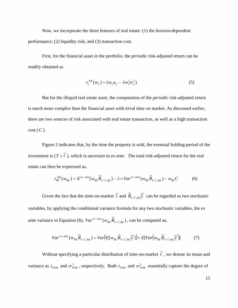
Now, we incorporate the three features of real estate: (1) the horizon-dependent
performance; (2) liquidity risk; and (3) transaction cost.
First, for the financial asset in the portfolio, the periodic risk-adjusted return can be
readily obtained as
)()( 22LLLLL
AdjL wuwwr σλ−= (5)
But for the illiquid real estate asset, the computation of the periodic risk-adjusted return
is much more complex than the financial asset with trival time on market. As discussed earlier,
there are two sources of risk associated with real estate transaction, as well as a high transaction
cost (C ).
Figure 2 indicates that, by the time the property is sold, the eventual holding-period of the
investment is ( tT ~+ ), which is uncertain in ex ante. The total risk-adjusted return for the real
estate can then be expressed as,
CwRwVarRwEwr REREtTREanteex
REtTREanteex
REAdj
RE −×−= +−
+− )~(]~[)( ,~,~ λ (6)
Given the fact that the time-on-market t~ and tR REtT~~
,~+ can be regarded as two stochastic
variables, by applying the conditional variance formula for any two stochastic variables, the ex
ante variance in Equation (6), )~( ,~ REtTREanteex RwVar +
− , can be computed as,
( ) ( )]~~[]~~[)~( ,~,~,~ tRwVarEtRwEVarRwVar REtTREREtTREREtTREanteex
+++− += (7)
Without specifying a particular distribution of time-on-market t~ , we denote its mean and
variance as TOMt and 2TOMσ , respectively. Both TOMt and 2
TOMσ essentially capture the degree of

16
real estate illiquidity. In terms of ex post return ( tR REtT~~
,~+ ), recent studies by Lin and Liu (2008)
and Cheng, Lin and Liu (2010a) find that the total return upon sale follows the distribution with
mean REutT )~( + and standard deviation REtT σ)~( + . We can thus simplify Equation (7) as
})(){()~( 222222,~ TOMRERERETOMREREtTRE
anteex utTwRwVar σσσ +++=+− (8)
Equation (8) integrates two source of risks in real estate investment, price risk and
liquidity risk ( TOMt , 2TOMσ ), into one unified risk metric.
For the ex ante expected return - the first term of Equation (6), first calculate the
expectation of the ex post expected return conditional on time-on-market ( t~ ), and then use the
Law of Iterated Expectations:
RETOMRE
RERE
REtTREREtTREanteex
utTw
utTwE
tRwEERwE
)(
])~([
]]~~[[]~[ ,~,~
+=
+=
= ++−
(9)
Substituting Equations (8) and (9) into Equation (6) yields
Cwu
tTwutTwwr
RERERETOM
RETOMRERETOMREREAdj
RE
−+
++−+=
)](
)[( )()(
222
222
σσ
σλ (10)
Therefore, the periodic risk-adjusted return for the illiquid real estate is
TOM
RETOM
RERETOMRETOMRERERERE
AdjRE tT
CwtT
utTwuwwr
+−
++
++−= ])(
)[( )(222
22 σσσλ (11)
17
For mathematical simplicity, we assume that the correlation between the real estate and
financial assets is zero, i.e., 0=ρ . Although this assumption may seem strong, it is not entirely
unreasonable as it has been well documented in the empirical studies that real estate historically
has low correlation with financial assets. For example, using annual U.S. data from 1947 to
1982, Ibbotson and Siegel (1984) found real estate's correlation with S&P stocks to be -0.06,
Worzala and Vandell (1993) estimate the correlation between NCREIF quarterly index from
1980 to 1991 and stocks of the same period to be about -0.0971. Eichholtz and Hartzell (1996)
document correlations between real estate and stock indexes to be -0.08 for U.S., -0.10 for
Canada, and -0.09 for U.K. Quan and Titman (1999) examined the correlation for 17 countries
and, unlike earlier studies, they find a generally positive correlation pattern in most countries, but
for the U.S. such positive correlation is insignificant.
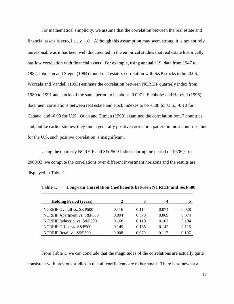
Using the quarterly NCREIF and S&P500 Indices during the period of 1978Q1 to
2008Q3, we compute the correlations over different investment horizons and the results are
displayed in Table 1.
Table 1. Long-run Correlation Coefficients between NCREIF and S&P500
Holding Period (years) 2 3 4 5
NCREIF Overall vs. S&P500 0.116 0.114 0.074 0.028 NCREIF Apartment vs. S&P500 0.094 0.078 0.069 0.074 NCREIF Industrial vs. S&P500 0.168 0.118 0.107 0.104 NCREIF Office vs. S&P500 0.149 0.165 0.142 0.115 NCREIF Retail vs. S&P500 -0.008 -0.079 -0.117 -0.107
From Table 1, we can conclude that the magnitudes of the correlations are actually quite
consistent with previous studies in that all coefficients are rather small. There is somewhat a
18
trend that the correlations seem to slightly decline as holding period increases. This result, along
with the findings by previous studies, reaffirms that real estate has low correlations with stocks
and provides some reasonable justifications to the assumption of zero correlation between real
estate and stocks in this study. 8
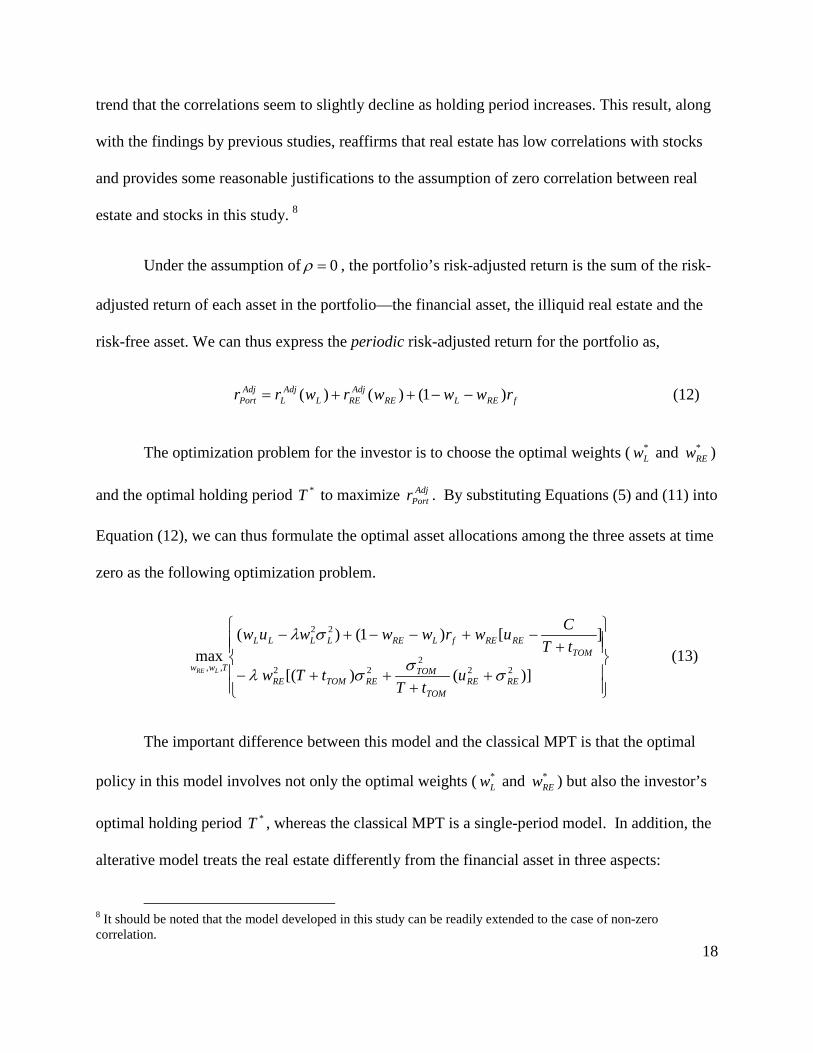
Under the assumption of 0=ρ , the portfolio’s risk-adjusted return is the sum of the risk-
adjusted return of each asset in the portfolio—the financial asset, the illiquid real estate and the
risk-free asset. We can thus express the periodic risk-adjusted return for the portfolio as,
fRELREAdj
RELAdj
LAdj
Port rwwwrwrr )1()()( −−++= (12)
The optimization problem for the investor is to choose the optimal weights ( *Lw and *
REw )
and the optimal holding period *T to maximize AdjPortr . By substituting Equations (5) and (11) into
Equation (12), we can thus formulate the optimal asset allocations among the three assets at time
zero as the following optimization problem.
++
++−
+−+−−+−
)]()[(
][)1()(max
222
22
22
,,RERE
TOM
TOMRETOMRE
TOMREREfLRELLLL
Tww utT
tTw
tTCuwrwwwuw
LRE σσσλ
σλ (13)
The important difference between this model and the classical MPT is that the optimal
policy in this model involves not only the optimal weights ( *Lw and *
REw ) but also the investor’s
optimal holding period *T , whereas the classical MPT is a single-period model. In addition, the
alterative model treats the real estate differently from the financial asset in three aspects:
8 It should be noted that the model developed in this study can be readily extended to the case of non-zero correlation.

19
(1) the model distinguishes the price behavior of real estate from that of financial assets
by recognizing the fact that real estate returns are not i.i.d.; (2) the real estate performance
requires a different measure from that of financial assets: the ex ante measure, which integrates
price risk with real estate liquidity risk, is the appropriate real estate performance measure; (3)
the model explicitly incorporates the high transaction cost of real estate.
Now suppose that real estate can be traded instantly with trivial time-on-market risk, i.e.,
0≈TOMt and 02 ≈TOMσ , and further suppose that the transaction cost is negligible when selling
real estate ( 0≈C ). Equation (13) can then be rewritten as
[ ]
+
−−−++2222,,
)1(max
LLRERE
fLRELLRERE
Tww wTw
rwwuwuwLRE σσλ
(14)
This is still different from the classical MPT as in Equation (3) with 0=ρ because of the
holding period T in Equation (14). However, we can readily show that the classical MPT holds
only when real estate returns are i.i.d.
We next solve the optimization problem in Equation (13). First, we take the partial
derivative of Equation (13) with respect to T, to obtain,
0)(
])(
)([ 22
22222 =
++
++
−−TOM
RE
TOM
RERETOMRERE tT
CwtT
uw σσσλ (15)
Similarly, the partial derivative of Equation (13) with respect to REw results in
0)]()[( 2 222
2 =++
++−+
−− RERETOM
TOMRETOMRE
TOMfRE u
tTtTw
tTCru σ
σσλ (16)

20
Equations (15) and (16) have two questions and two unknown variables: REw and T . We
can solve the optimal real estate allocation ( *REw ) and the optimal holding period ( *T )
simultaneously. The existence of the optimal holding period suggests that the optimal mixed-
asset allocation is related to the investor’s holding period. In contrast, the classical MPT only
solves a single-period optimization problem and implies that the optimal asset allocation is
independent of holding-period. To obtain a closed-form solution to Eequations (15) and (16) is
not easy, but we can examine some important properties of the optimal holding-period (T*).
From Equation (15), we have
22
222
)(
)(RERE
TOM
RERETOMRE wtT
Cuw σλσσλ=
+++ . (17)
Hence,
2
222*
)(
RERE
RERETOMRETOM w
CuwtTσλ
σσλ ++=+ . (18)
Therefore,
0
)( 2
1
2
2222
*
>++
=∂∂
RERE
RERETOMRERERE w
CuwwCT
σλσσλσλ
(19)
0)
)((
)(2
12
22
2
2222
*
>+
++=
∂∂
RE
RERE
RERE
RERETOMRETOM
u
wCuw
Tσσ
σλσσλσ
(20)

21
0)
(
)(2
144
22
2
2222
*
<−−++
=∂∂
RERERE
RETOM
RERE
RERETOMRERE wCu
wCuw
Tσλσ
σ
σλσσλσ
(21)
These results can be summarized in Theorem 1.
Theorem 1. Real estate transaction cost, liquidity risk, and price risk play a crucial role in
determining the optimal holding period. In particular, we have
0 ;0 ;0 2
*
2
**
<∂∂
>∂∂
>∂∂
RETOM
TTCT
σσ
Other things being equal, a less liquid market (a larger 2TOMσ ) with a higher
transaction cost (higher C ) implies a longer optimal holding period. However, a higher price
volatility ( 2REσ ) implies a shorter optimal holding period.
The important insight revealed by Theorem 1 is that the optimal holding period is
determined by both systematic and non-systematic factors—market condition ( 2TOMσ and C) and
property-specific risk ( 2REσ ). This is consistent with the findings by a recent study of Cheng, Lin
and Liu (2010b), which concludes that the holding period of real estate is affected by both
market conditions and property-specific performance. Theorem 1 is also consistent with the
findings by Mayshar (1979) and Constantinides (1986), both of which find that even a small
transaction cost results in a longer holding period with fewer assets (as opposed to the market
portfolio).
With the optimal holding-period ( *T ), we can readily solve the optimal weight of real
estate ( *REw ) by using Equation (16), which can be summarized in Theorem 2.

22
Theorem 2. The optimal weight on the real estate ( *REw ) is given by,
)]()[(2 22
*
22*
**
RERETOM
TOMRETOM
TOMfRE
RE
utT
tT
tTCru
wσσσλ +
+++
+−−
= (22)
In addition, *REw is negatively related to real estate liquidity risk and its transaction cost, i.e.,
(a). 0*
<∂∂
CwRE ; (b). 0
*
<∂∂
TOM
REwσ
.
Two conclusions can be drawn from Theorem 2. First, Modern Portfolio Theory, which
implicitly assumes that all assets have zero time-on-market risk, is not directly applicable to
mixed-asset portfolios that include real estate. Second, by taking the liquidity risk, high
transaction cost, and non-i.i.d. nature of real estate returns into consideration, we demonstrate
that optimal real estate allocation is affected by liquidity risk, investor time horizon and real
estate transaction cost. In particular, the optimal weight on the real estate asset is always less
than that suggested by the classical MPT. In other words, the optimal real state allocation
suggested by pervious literature is exaggerated.
5. A Numerical Example
In this section, we use an example to study how we can numerically solve both the
optimal real estate allocation and the optimal holding period.
From Equation (22), we have

23
)]()[(2 22
*
22*
**
RERETOM
TOMRETOM
TOMfRE
RE
utT
tT
tTCru
wσσσλ +
+++
+−−
= (22')
and from Equation (18), we have
2*
222** )(
RERE
RERETOMRETOM w
CuwtTσλ
σσλ ++=+ . (18')
Substituting Equation (18') into Equation (22'), we can obtain an equation of only one
unknown variable ( *REw ). To obtain a closed form solution for *
REw is difficult. However, we can
find a numerical solution if we have all the model parameters: (1) real estate illiquidity, i.e., TOMt
and 2TOMσ ; (2) the periodic return and risk of real estate asset, REu and REσ ; and (3) the
transaction cost ( C ), the risk-free rate ( fr ), and the risk aversion parameter (λ ). Now we
discuss these parameters in turn.
1. Real estate illiquidity. Although not required for model development, the distribution
of TOM needs to be reasonably assumed in order to estimate TOMt and 2TOMσ . Following Cheng,
Lin, and Liu (2010a), we assume the distribution of TOM to be negative exponential for
demonstration purposes. The negative exponential distribution has a simple mathematical
property: its variance is equal to the square of its mean. Therefore, the variance of the time-on-
market (TOM) is equal to the square of the expected TOM, i.e., 22TOMTOM t=σ . In addition, based
on information from the National Association of Realtors, the average TOM for the US
residential market during the period from 1982 to 2010 was about 7.5 months. Considering the
24
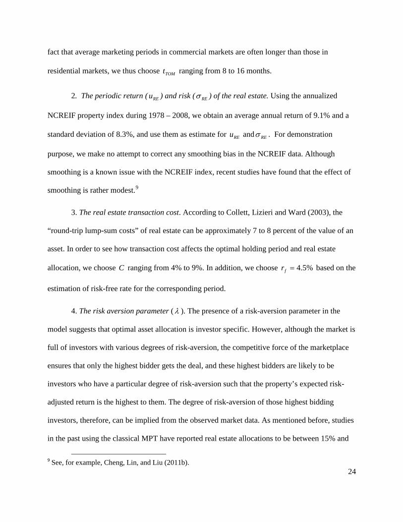
fact that average marketing periods in commercial markets are often longer than those in
residential markets, we thus choose TOMt ranging from 8 to 16 months.
2. The periodic return ( REu ) and risk ( REσ ) of the real estate. Using the annualized
NCREIF property index during 1978 – 2008, we obtain an average annual return of 9.1% and a
standard deviation of 8.3%, and use them as estimate for REu and REσ . For demonstration
purpose, we make no attempt to correct any smoothing bias in the NCREIF data. Although
smoothing is a known issue with the NCREIF index, recent studies have found that the effect of
smoothing is rather modest.9
3. The real estate transaction cost. According to Collett, Lizieri and Ward (2003), the
“round-trip lump-sum costs” of real estate can be approximately 7 to 8 percent of the value of an
asset. In order to see how transaction cost affects the optimal holding period and real estate
allocation, we choose C ranging from 4% to 9%. In addition, we choose %5.4=fr based on the
estimation of risk-free rate for the corresponding period.
4. The risk aversion parameter (λ ). The presence of a risk-aversion parameter in the
model suggests that optimal asset allocation is investor specific. However, although the market is
full of investors with various degrees of risk-aversion, the competitive force of the marketplace
ensures that only the highest bidder gets the deal, and these highest bidders are likely to be
investors who have a particular degree of risk-aversion such that the property’s expected risk-
adjusted return is the highest to them. The degree of risk-aversion of those highest bidding
investors, therefore, can be implied from the observed market data. As mentioned before, studies
in the past using the classical MPT have reported real estate allocations to be between 15% and
9 See, for example, Cheng, Lin, and Liu (2011b).

25
40%.10 If we take the middle point of this range, 27% for instance, it will imply a risk-aversion
parameter 12=λ , according to Equation (4) with 0=ρ .
With the model parameters at hand, we can obtain numerical solutions to *REw and *T .
The results are reported in Tables 2 and 3.
Table 2. The Optimal Holding Period of Real Estate
8 months 10 months 12 months 14 months 16 months4% 3.0 3.2 3.4 3.6 3.85% 3.5 3.7 3.9 4.1 4.36% 4.1 4.3 4.5 4.6 4.87% 4.7 4.9 5.0 5.2 5.48% 5.3 5.5 5.6 5.8 5.99% 6.0 6.1 6.2 6.4 6.510% 6.6 6.7 6.8 6.9 7.1
Transaction Cost
Expected TOM
Note: This table displays the optimal holding period (T* + tTOM) under various
assumptions of transaction cost and TOM. All numbers are in years unless noted. Tables 2 is quite consistent with the finding by Cheng, Lin and Liu. (2010b)
Table 3. The Optimal Weights for Real Estate
8 months 10 months12 months14 months16 months4% 5.87% 5.45% 5.05% 4.69% 4.37%5% 4.97% 4.69% 4.42% 4.16% 3.92%6% 4.29% 4.10% 3.91% 3.72% 3.54%7% 3.76% 3.63% 3.49% 3.35% 3.21%8% 3.34% 3.25% 3.15% 3.04% 2.93%9% 3.01% 2.94% 2.86% 2.78% 2.69%10% 2.73% 2.67% 2.62% 2.55% 2.48%
Transaction Cost
Expected TOM
Note: This table displays the optimal weights of real estate given the corresponding
optimal holding-periods in Table 2.
10 Numerous academic studies since the 1980s often conclude that real estate should constitute 15% to 40% or more of a diversified portfolio. See, for example, Hartzell, Hekman and Miles (1986), Fogler (1984), Firstenberg, Ross and Zisler (1988), and Hudson-Wilson, Fabozzi and Gordon (2005), among others.

26
From Table 2, the expected optimal holding period for real estate ranges from three to
seven years, depending on market condition (degree of illiquidity) and transaction cost. The
optimal holding periods are longer when transaction costs are high and/or the time-on-market is
expected to be longer, which is consistent with the findings of previous studies in the finance
literature. The numerical results in Table 2 are also in line with the empirical finding by Gau and
Wang (1994), and reasonably close to the finding by Collett, Lizieri and Ward (2003).
The main point of interest, of course, is the optimal real estate allocation displayed in
Table 3, which ranges from 2.48% to 5.87%. Compared to previous findings based on the
classical MPT, these real estate allocations are much more in line with the institutional portfolio
reality. Clearly, the optimal allocation to real estate is determined by investment horizon,
liquidity risk and transaction cost. Holding other things equal, higher transaction cost and higher
liquidity risk (longer TOM) correlate with lower real estate allocations. These results suggest
that the alternative model is able to provide a viable solution to the long-standing real estate
allocation puzzle.
It may be of interest to compare our approach and results with a few recent studies that
have attempted at resolving the real estate allocation puzzle. MacKinnon and Zaman (2009)
examine the effect of long investment horizon on optimal real estate allocation using the VAR
model developed in Campbell and Viceira (2005). Applying the model to U.S. property data,
they find that, although real estate does exhibit long-run mean-reversion, the behavior is weaker
than equities, which means real estate is almost as risky as equities in the long-run. But despite
of this, they find the optimal allocations to real estate remains rather high (17- 31%) and has the
tendency to be higher as the investment horizon gets longer. Rehring (2011) adopt the same
Campbell-Viceira method to examine U.K. commercial property data. Unlike MacKinnon and
27
Zaman (2009), he finds that the model-predicted real estate returns to exhibit decreasing variance
in the longer horizon, which is consistent with his finding that the optimal real estate allocation
increases rather rapidly as holding period prolongs. Therefore, neither study is able to resolve
the real estate allocation puzzle. In contrast, using a somewhat different auto-regression model,
Pagliari (2011) finds that, although real estate variance “decays” over the long-run, the variance
of financial asset decays faster, thus making real estate relatively more risky as holding period
gets longer. This finding, accompanied by what he finds to be increased correlation between
private and public assets in the long run, causes real estate to be less appealing and thus carry
less weight in mixed-asset portfolios. He suggests about 12% allocation in real estate for
investors with a four-year investment horizon, which is still much higher than the reported 3-5%
institutional reality. None of these three studies addresses real estate liquidity risk. In an effort
to incorporate illiquidity into mixed-asset portfolio decision, Anglin and Gao (2011) develops a
model to discuss the impact of liquidity and liquidity shock on portfolio. But they did not
provide what the optimal real estate weight should be.
The differences between our approach and these afore-mentioned studies are obvious.
First, the approaches of MacKinnon and Zaman (2009), Rehring (2011) and Pagliari (2011)
essentially remain in the realm of empirically modifying the way MPT is applied to real estate,
that is, they attempt to “fine-tune” the way we use MPT, not MPT itself. Our approach, on the
other hand, is to modify the theory by extending it to explicitly accommodate the unique real
estate features based on multi-period utility maximization. Second, while the studies above focus
on exploring better empirical approaches for estimating the input data (long-run mean and
variances) to MPT, we focus on developing an alternative model by explicitly incorporate unique
features of real estate.
28
5. Conclusions
Modern Portfolio Theory (MPT) is a single-period asset allocation model. Its validity on
multi-period portfolio decisions hinges on a critical assumption – an efficient market where asset
returns are independent and identically distributed (i.i.d.) over time. Because real estate does not
fit in this paradigm, the classical MPT needs to be extended to accommodate the more complex
features of real estate and mixed-asset portfolio analysis. Building upon a series of recent
research on real estate illiquidity and performance metrics, this paper synthesizes some of the
latest advances in the literature to develop an alternative model that extends the classical MPT
for mixed-asset portfolio analysis. Unlike many previous efforts that attempt to empirically solve
the real estate allocation puzzle with ad hoc solutions, we provide a formal model that explicitly
incorporates the three most unique features of real estate – horizon-dependent performance,
liquidity risk and high transaction cost – into a multi-period mean-variance analysis. Using
commercial real estate data, the alternative model produces a range of optimal real estate
allocations that are quite in line with the reality of institutional portfolios.
It should be acknowledged that, although our model is able to succeed where the
conventional approach has failed in resolving the long-standing real estate allocation puzzle, this
work should only be viewed as a first step in the search for a more general portfolio theory for
mixed-asset portfolio analysis. Many issues still remain. To mention a few: First, we have
implicitly assumed that the investors are “normal” sellers who are not under any liquidity shock
to force liquidation of real estate. A more general theory should incorporate seller heterogeneity
and the possibility of liquidity shock into the model. Second, we do not consider the
indivisibility or partial sale of real estate asset. We assume the entire real estate holding will be
sold together. In reality, investors facing liquidity shock may need to liquidate only part of their
29
real estate holdings to satisfy the need for cash. This issue is discussed in Anglin and Gao (2011)
to some extent. Third, while the alternative model breaks away from the efficient market
paradigm in which asset prices are assumed to follow the random walk, it is still confined within
the mean-variance framework, which implicitly assumes that investors have a symmetric
aversion to price volatility. The reality, though, is that investor’s risk perception is often
asymmetric. To the extent that asset returns are not jointly normally-distributed, the concept of
downside-risk is an appealing risk metric (and more complex as well). This, of course, is a much
broader issue that pertains to nearly all mainstream finance theories as well. Despite these
simplifications, the empirical analysis and theoretical exploration accomplish the two modest
objectives of this paper—to extend the MPT for mixed-asset portfolio analysis and to suggest a
solution to the decades-old real estate allocation puzzle. While this line of work is certainly at the
stage of early exploration, the prospect is promising.
30
References
Amihud, Y. and H. Mendelson (1986), “Asset Pricing and the Bid-ask Spread,” Journal of Financial Economics, 223-249. Anglin, P. and Y. Gao (2011), “Integrating Illiquid Assets into the Portfolio Decision Process,” Real Estate Economics 39 (2): 277-311. Atkins, A. and E. Dyl. (1997), “Transactions Costs and Holding Period for Common Stocks,” Journal of Finance: 309-325. Bond, S., S. Hwang, Z. Lin and K. Vandell (2007), “Marketing Period Risk in a Portfolio Context: Theory and Empirical Estimates from the UK Commercial Real Estate Market?” Journal of Real Estate Finance and Economics 34: 447-461.
Brennan, M. (1975), “The Optimal Number of Securities in a Risky Asset Portfolio When There Are Fixed Costs of Transacting: Theory and Some Empirical Results,” Journal of Financial and Quantitative Analysis: 483-496. Brock, W., D. Dechert and J. Scheinkman (1987), “A Test for Independence Based Upon the Correlation Dimension,” Working Paper, University of Wisconsin-Madison Case, K. and R. Shiller, (1989), “The Efficiency of the Market for Single-Family Homes,” American Economic Review 79: 125-137 Cheng, P., Z. Lin and Y. Liu (2010a), “Illiquidity and Portfolio Risk of Thinly Traded Assets,” Journal of Portfolio Management Vol. 36, No 2, p 126-138 Cheng, P., Z. Lin and Y. Liu (2010b), “Illiquidity, Transaction Cost, and Optimal Holding Period for Real Estate: Theory and Application,” Journal of Housing Economics, Vol. 19, 109-118. Cheng, P., Z. Lin and Y. Liu (2011a), “Has Real Estate Come of Age?” Journal of Real Estate Portfolio Management, forthcoming. Cheng, P., Z. Lin and Y. Liu (2011b), “Heterogeneous Information and Appraisal Smoothing,” Journal of Real Estate Research, Vol. 33 (4). Clifford A., R. Krail and J. Liew (2001), “Do hedge funds hedge?” Journal of Portfolio Management, 28:1, 6 – 19. Collett, D., C. Lizieri, and C. Ward (2003), “Timing and the Holding Periods of Institutional Real Estate,” Real Estate Economics, 31 (2), 205-222. Constantinides, G. (1986), “Capital Market Equilibrium with Transaction Costs,” Journal of Political Economy 94, 842-862.

31
Englund, P., T. Gordon, and J. Quigley (1999), “The Valuation of Real Capital: A Random Walk down Kungsgatan,” Journal of Housing Economics 8: 205-216. Fama, E., (1970), “Multi-period Consumption-Investment Decisions,” American Economic Review, 163- 174. Firstenberg P., S. Ross and R. Zisler (1988), “Real Estate: The Whole Story,” Journal of Portfolio Management 14(3), 22-34. Fogler, H. (1984), "20% in real estate: can theory justify it?" Journal of Portfolio Management, Vol. 7, 6-13. Gao, A., Z. Lin and C. Na. (2009), “Housing Market Dynamics: Evidence of Mean Reversion and Downward Rigidity,” Journal of Housing Economics, Special Issue, Vol. 18: 256-266. Gau, G. and K. Wang (1990), “Capital Structure Decisions in Real Estate Investment,” AREUEA Journal 18:501-521. Goetzmann, W. and R. Dhar (2005), “Institutional Perspectives on Real Estate Investing: The Role of Risk and Uncertainty,” Yale ICF Working Paper No. 05-20 Graff, R., A. Harrington and M. Young (1997), “The Shape of Australian Real Estate Return Distributions and Comparisons to the United States,” Journal of Real Estate Research, 14:3, 291–308. Hartzell, D., J. Heckman and M. Miles (1986), “Diversification Categories in Investment Real Estate”, AREUEA journal, 14, 230-254 Hudson-Wilson, S., F. Fabozzi and J. Gordon (2005) “Why Real Estate,” Journal of Portfolio Management: Special Real Estate Issue, 12–24. Lin, Z. and Y. Liu (2008), “Real Estate Returns and Risk with Heterogeneous Investors,” Real Estate Economics 36, 753-776. Lin, Z., Y. Liu and K. Vandell (2009), “Marketing Period Risk in a Portfolio Context: Comment and Extension,” Journal of Real Estate Finance and Economics, 38, 183-191. Lippman, S. and J. McCall (1986), “An Operational Measure of Liquidity,” American Economic Review 76, 43-55. Lusht, K. (1988), “The Real Estate Pricing Puzzle,” AREUEA Journal 16 (2): 95-104. MacKinnon, G. and A. Zaman (2009), “Real Estate for the Long Term: The Effect of Return Predicatability on Long-Horizon Allocations,” Real Estate Economics, 37 (1), 117-153. Markowitz, H. (1952), "Portfolio Selection," The Journal of Finance 7 (1), 77–91.
32
Mayshar, J. (1979), “Transaction Costs in a Model of Capital Market Equilibrium,” Journal of Political Economy 87, 673-700. Merton, R. (1969), “Lifetime Portfolio Selection under Uncertainty: The Continuous Time Case”, Review of Economics and Statistics, 51, 247-257. Quan, D. and S. Titman (1999). “Do Real Estate Prices and Stock Prices Move Together? An International Analysis”, Real Estate Economics, 27:3. 183-207. Pagliari, J. (2011), “Long-Run Investment Horizons and Mixed-Asset Portfolio Allocations,” Working Paper, University of Chicago. Rehring, C. (2011), “Real Estate in a Mixed-Asset Portfolio: The Role of the Investment Horizon,” Real Estate Economics, 1-31. Samuelson, P. (1969), “Lifetime Portfolio Selection by Dynamic Stochastic Programming,” Review of Economics and Statistics, 51, 239-246 Sharpe, W. (1963), “A Simplified Model for Portfolio Analysis,” Management Science 9: 277-93 Young, M. and R. Graff (1995), “Real Estate is Not Normal: A Fresh Look at Real Estate Return Distributions,” Journal of Real Estate Finance and Economics 10, 225-259. Young, M. (2008) “Revisiting Non-normal Real Estate Return Distributions by Property Type in the U.S.,” Journal of Real Estate Finance and Economics, 36:2, 233-48. Young, M, S. Lee and S. Devaney, (2006), “Non-normal Real Estate Return Distributions by Property Type in the U.K.,” Journal of Property Research, 23:2, 109–133.