optimal time-domain noise reduction filters
DESCRIPTION
A Theoretical StudyTRANSCRIPT


SpringerBriefs in Electrical and ComputerEngineering
For further volumes:http://www.springer.com/series/10059


Jacob Benesty • Jingdong Chen
Optimal Time-Domain NoiseReduction Filters
A Theoretical Study
123

Prof. Dr. Jacob BenestyINRS-EMTUniversity of Quebecde la Gauchetiere Ouest 800Montreal, H5A 1K6, QCCanadae-mail: [email protected]
Jingdong ChenNorthwestern Polytechnical University127 Youyi West RoadXi’an, Shanxi 710072Chinae-mail: [email protected]
ISSN 2191-8112 e-ISSN 2191-8120
ISBN 978-3-642-19600-3 e-ISBN 978-3-642-19601-0
DOI 10.1007/978-3-642-19601-0
Springer Heidelberg Dordrecht London New York
� Jacob Benesty 2011
This work is subject to copyright. All rights are reserved, whether the whole or part of the material isconcerned, specifically the rights of translation, reprinting, reuse of illustrations, recitation, broadcast-ing, reproduction on microfilm or in any other way, and storage in data banks. Duplication of thispublication or parts thereof is permitted only under the provisions of the German Copyright Law ofSeptember 9, 1965, in its current version, and permission for use must always be obtained fromSpringer. Violations are liable to prosecution under the German Copyright Law.
The use of general descriptive names, registered names, trademarks, etc. in this publication does notimply, even in the absence of a specific statement, that such names are exempt from the relevantprotective laws and regulations and therefore free for general use.
Cover design: eStudio Calamar, Berlin/Figueres
Printed on acid-free paper
Springer is part of Springer Science+Business Media (www.springer.com)

Contents
1 Introduction . . . . . . . . . . . . . . . . . . . . . . . . . . . . . . . . . . . . . . . . 11.1 Noise Reduction . . . . . . . . . . . . . . . . . . . . . . . . . . . . . . . . . . 11.2 Organization of the Work . . . . . . . . . . . . . . . . . . . . . . . . . . . . 2References . . . . . . . . . . . . . . . . . . . . . . . . . . . . . . . . . . . . . . . . . . 2
2 Single-Channel Noise Reduction with a Filtering Vector . . . . . . . . 32.1 Signal Model . . . . . . . . . . . . . . . . . . . . . . . . . . . . . . . . . . . . 32.2 Linear Filtering with a Vector. . . . . . . . . . . . . . . . . . . . . . . . . 52.3 Performance Measures . . . . . . . . . . . . . . . . . . . . . . . . . . . . . . 6
2.3.1 Noise Reduction . . . . . . . . . . . . . . . . . . . . . . . . . . . . . 62.3.2 Speech Distortion . . . . . . . . . . . . . . . . . . . . . . . . . . . . 82.3.3 Mean-Square Error (MSE) Criterion . . . . . . . . . . . . . . . 9
2.4 Optimal Filtering Vectors . . . . . . . . . . . . . . . . . . . . . . . . . . . . 112.4.1 Maximum Signal-to-Noise Ratio (SNR). . . . . . . . . . . . . 122.4.2 Wiener. . . . . . . . . . . . . . . . . . . . . . . . . . . . . . . . . . . . 122.4.3 Minimum Variance Distortionless Response (MVDR) . . . 142.4.4 Prediction. . . . . . . . . . . . . . . . . . . . . . . . . . . . . . . . . . 162.4.5 Tradeoff. . . . . . . . . . . . . . . . . . . . . . . . . . . . . . . . . . . 172.4.6 Linearly Constrained Minimum Variance (LCMV) . . . . . 182.4.7 Practical Considerations . . . . . . . . . . . . . . . . . . . . . . . . 20
2.5 Summary . . . . . . . . . . . . . . . . . . . . . . . . . . . . . . . . . . . . . . . 20References . . . . . . . . . . . . . . . . . . . . . . . . . . . . . . . . . . . . . . . . . . 21
3 Single-Channel Noise Reduction with a RectangularFiltering Matrix . . . . . . . . . . . . . . . . . . . . . . . . . . . . . . . . . . . . . . 233.1 Linear Filtering with a Rectangular Matrix . . . . . . . . . . . . . . . . 233.2 Joint Diagonalization . . . . . . . . . . . . . . . . . . . . . . . . . . . . . . . 26
v

3.3 Performance Measures . . . . . . . . . . . . . . . . . . . . . . . . . . . . . . 273.3.1 Noise Reduction . . . . . . . . . . . . . . . . . . . . . . . . . . . . . 273.3.2 Speech Distortion . . . . . . . . . . . . . . . . . . . . . . . . . . . . 283.3.3 MSE Criterion . . . . . . . . . . . . . . . . . . . . . . . . . . . . . . 28
3.4 Optimal Rectangular Filtering Matrices . . . . . . . . . . . . . . . . . . 313.4.1 Maximum SNR. . . . . . . . . . . . . . . . . . . . . . . . . . . . . . 313.4.2 Wiener. . . . . . . . . . . . . . . . . . . . . . . . . . . . . . . . . . . . 333.4.3 MVDR . . . . . . . . . . . . . . . . . . . . . . . . . . . . . . . . . . . 353.4.4 Prediction. . . . . . . . . . . . . . . . . . . . . . . . . . . . . . . . . . 363.4.5 Tradeoff. . . . . . . . . . . . . . . . . . . . . . . . . . . . . . . . . . . 373.4.6 Particular Case: M = L . . . . . . . . . . . . . . . . . . . . . . . . 383.4.7 LCMV. . . . . . . . . . . . . . . . . . . . . . . . . . . . . . . . . . . . 40
3.5 Summary . . . . . . . . . . . . . . . . . . . . . . . . . . . . . . . . . . . . . . . 40References . . . . . . . . . . . . . . . . . . . . . . . . . . . . . . . . . . . . . . . . . . 40
4 Multichannel Noise Reduction with a Filtering Vector. . . . . . . . . . 434.1 Signal Model . . . . . . . . . . . . . . . . . . . . . . . . . . . . . . . . . . . . 434.2 Linear Filtering with a Vector. . . . . . . . . . . . . . . . . . . . . . . . . 454.3 Performance Measures . . . . . . . . . . . . . . . . . . . . . . . . . . . . . . 46
4.3.1 Noise Reduction . . . . . . . . . . . . . . . . . . . . . . . . . . . . . 474.3.2 Speech Distortion . . . . . . . . . . . . . . . . . . . . . . . . . . . . 484.3.3 MSE Criterion . . . . . . . . . . . . . . . . . . . . . . . . . . . . . . 49
4.4 Optimal Filtering Vectors . . . . . . . . . . . . . . . . . . . . . . . . . . . . 514.4.1 Maximum SNR. . . . . . . . . . . . . . . . . . . . . . . . . . . . . . 514.4.2 Wiener. . . . . . . . . . . . . . . . . . . . . . . . . . . . . . . . . . . . 524.4.3 MVDR . . . . . . . . . . . . . . . . . . . . . . . . . . . . . . . . . . . 554.4.4 Space–Time Prediction . . . . . . . . . . . . . . . . . . . . . . . . 564.4.5 Tradeoff. . . . . . . . . . . . . . . . . . . . . . . . . . . . . . . . . . . 574.4.6 LCMV. . . . . . . . . . . . . . . . . . . . . . . . . . . . . . . . . . . . 58
4.5 Summary . . . . . . . . . . . . . . . . . . . . . . . . . . . . . . . . . . . . . . . 59References . . . . . . . . . . . . . . . . . . . . . . . . . . . . . . . . . . . . . . . . . . 59
5 Multichannel Noise Reduction with a RectangularFiltering Matrix . . . . . . . . . . . . . . . . . . . . . . . . . . . . . . . . . . . . . . 615.1 Linear Filtering with a Rectangular Matrix . . . . . . . . . . . . . . . . 615.2 Joint Diagonalization . . . . . . . . . . . . . . . . . . . . . . . . . . . . . . . 635.3 Performance Measures . . . . . . . . . . . . . . . . . . . . . . . . . . . . . . 64
5.3.1 Noise Reduction . . . . . . . . . . . . . . . . . . . . . . . . . . . . . 645.3.2 Speech Distortion . . . . . . . . . . . . . . . . . . . . . . . . . . . . 655.3.3 MSE Criterion . . . . . . . . . . . . . . . . . . . . . . . . . . . . . . 65
vi Contents

5.4 Optimal Filtering Matrices . . . . . . . . . . . . . . . . . . . . . . . . . . . 675.4.1 Maximum SNR. . . . . . . . . . . . . . . . . . . . . . . . . . . . . . 675.4.2 Wiener. . . . . . . . . . . . . . . . . . . . . . . . . . . . . . . . . . . . 695.4.3 MVDR . . . . . . . . . . . . . . . . . . . . . . . . . . . . . . . . . . . 715.4.4 Space–Time Prediction . . . . . . . . . . . . . . . . . . . . . . . . 715.4.5 Tradeoff. . . . . . . . . . . . . . . . . . . . . . . . . . . . . . . . . . . 725.4.6 LCMV. . . . . . . . . . . . . . . . . . . . . . . . . . . . . . . . . . . . 74
5.5 Summary . . . . . . . . . . . . . . . . . . . . . . . . . . . . . . . . . . . . . . . 75References . . . . . . . . . . . . . . . . . . . . . . . . . . . . . . . . . . . . . . . . . . 75
Index . . . . . . . . . . . . . . . . . . . . . . . . . . . . . . . . . . . . . . . . . . . . . . . . 77
Contents vii


Chapter 1Introduction
1.1 Noise Reduction
Signal enhancement is a fundamental topic of signal processing in general andof speech processing in particular [1]. In audio and speech applications such ascell phones, teleconferencing systems, hearing aids, human–machine interfaces, andmany others, the microphones installed in these systems always pick up some inter-ferences that contaminate the desired speech signal. Depending on the mechanismthat generates them, these interferences can be broadly classified into four basiccategories: additive noise originating from various ambient sound sources, interfer-ence from concurrent competing speakers, filtering effects caused by room surfacereflections and spectral shaping of recording devices, and echo from coupling be-tween loudspeakers and microphones. These four categories of distortions interferewith the measurement, processing, recording, and communication of the desiredspeech signal in very distinct ways and combating them has led to four im-portant research areas: noise reduction (also called speech enhancement), sourceseparation, speech dereverberation, and echo cancellation and suppression. A broadcoverage of these research areas can be found in [2, 3]. This work is devoted to thetheoretical study of the problem of speech enhancement in the time domain.
Noise reduction consists of recovering a speech signal of interest from the micro-phone signals, which are corrupted by unwanted additive noise. By additive noisewe mean that the signals picked up by the microphones are a superposition of theconvolved clean speech and noise. Schroeder at Bell Laboratories in 1960 was thefirst to propose a single-channel algorithm for that purpose [4]. It was basically aspectral subtraction method implemented with analog circuits.
Frequency-domain approaches are usually preferred in real-time applications asthey can be implemented efficiently thanks to the fast Fourier transform. However,they come with some well-known problems such as the so-called “musical noise,”which is very unpleasant to hear and difficult to get rid off. In the time domain, thisproblem does not exist and, contrary to what some readers might believe, time-domainalgorithms are at least as flexible as their counterparts in the frequency domain as it
J. Benesty and J. Chen, Optimal Time-Domain Noise Reduction Filters, 1SpringerBriefs in Electrical and Computer Engineering, 1,DOI: 10.1007/978-3-642-19601-0_1, © Jacob Benesty 2011

2 1 Introduction
will be shown throughout this work; but they can be computationally more complexin terms of multiplications. However, with little effort, it is not hard to make themmore efficient by exploiting the Toeplitz or close-to-Toeplitz structure of the matricesinvolved in these algorithms.
In this work, we propose a general framework for the time-domain noise reductionproblem. Thanks to this formulation, it is easy to derive, study, and analyze all kindsof algorithms.
1.2 Organization of the Work
The material in this work is organized into five chapters, including this one. Thefocus is on the time-domain algorithms for both the single and multiple microphonecases. The work discussed in these chapters is as follows.
In Chap. 2, we study the noise reduction problem with a single microphone byusing a filtering vector for the estimation of the desired signal sample.
Chapter 3 generalizes the ideas of Chap. 2 with a rectangular filtering matrix forthe estimation of the desired signal vector.
In Chap. 4, we study the speech enhancement problem with a microphone arrayby using a long filtering vector.
Finally, Chap. 5 extends the results of Chap. 4 with a rectangular filtering matrix.
References
1. J. Benesty, J. Chen, Y. Huang, I. Cohen, Noise Reduction in Speech Processing (Springer, Berlin,2009)
2. J. Benesty, J. Chen, Y. Huang, Microphone Array Signal Processing (Springer, Berlin, 2008)3. Y. Huang, J. Benesty, J. Chen, Acoustic MIMO Signal Processing (Springer, Berlin, 2006)4. M.R. Schroeder, Apparatus for suppressing noise and distortion in communication signals, U.S.
Patent No. 3,180,936, filed 1 Dec 1960, issued 27 Apr 1965

Chapter 2Single-Channel Noise Reduction witha Filtering Vector
There are different ways to perform noise reduction in the time domain. The simplestway, perhaps, is to estimate a sample of the desired signal at a time by applying afiltering vector to the observation signal vector. This approach is investigated inthis chapter and many well-known optimal filtering vectors are derived. We start byexplaining the single-channel signal model for noise reduction in the time domain.
2.1 Signal Model
The noise reduction problem considered in this chapter and Chap. 3 is one of recov-ering the desired signal (or clean speech) x(k), k being the discrete-time index, ofzero mean from the noisy observation (microphone signal) [1–3]
y(k) = x(k) + v(k), (2.1)
where v(k), assumed to be a zero-mean random process, is the unwanted additivenoise that can be either white or colored but is uncorrelated with x(k). All signalsare considered to be real and broadband. To simplify the derivation of the optimalfilters, we further assume that the signals are Gaussian and stationary.
The signal model given in (2.1) can be put into a vector form by considering theL most recent successive samples, i.e.,
y(k) = x(k) + v(k), (2.2)
where
y(k) = [y(k) y(k − 1) · · · y(k − L + 1)]T (2.3)
is a vector of length L, superscript T denotes transpose of a vector or a matrix,and x(k) and v(k) are defined in a similar way to y(k). Since x(k) and v(k) are
J. Benesty and J. Chen, Optimal Time-Domain Noise Reduction Filters, 3SpringerBriefs in Electrical and Computer Engineering, 1,DOI: 10.1007/978-3-642-19601-0_2, © Jacob Benesty 2011

4 2 Single-Channel Filtering Vector
uncorrelated by assumption, the correlation matrix (of size L × L) of the noisysignal can be written as
Ry = E[y(k)yT (k)
]
= Rx + Rv, (2.4)
where E[·] denotes mathematical expectation, and Rx = E[x(k)xT (k)
]and Rv =
E[v(k)vT (k)
]are the correlation matrices of x(k) and v(k), respectively. The objec-
tive of noise reduction in this chapter is then to find a “good” estimate of the samplex(k) in the sense that the additive noise is significantly reduced while the desiredsignal is not much distorted.
Since x(k) is the signal of interest, it is important to write the vector y(k) as anexplicit function of x(k). For that, we need first to decompose x(k) into two orthog-onal components: one proportional to the desired signal, x(k), and the other onecorresponding to the interference. Indeed, it is easy to see that this decomposition is
x(k) = ρxx · x(k) + xi(k), (2.5)
where
ρxx = [1 ρx (1) · · · ρx (L − 1)]T
= E [x(k)x(k)]
E[x2(k)
] (2.6)
is the normalized [with respect to x(k)] correlation vector (of length L) betweenx(k) and x(k),
ρx (l) = E [x(k − l)x(k)]
E[x2(k)
] , l = 0, 1, . . . , L − 1 (2.7)
is the correlation coefficient between x(k − l) and x(k),
xi(k) = x(k) − ρxx · x(k) (2.8)
is the interference signal vector, and
E [xi(k)x(k)] = 0L×1, (2.9)
where 0L×1 is a vector of length L containing only zeroes.Substituting (2.5) into (2.2), the signal model for noise reduction can be expressed
as
y(k) = ρxx · x(k) + xi(k) + v(k). (2.10)
This formulation will be extensively used in the following sections.

2.2 Linear Filtering with a Vector 5
2.2 Linear Filtering with a Vector
In this chapter, we try to estimate the desired signal sample, x(k), by applying afinite-impulse-response (FIR) filter to the observation signal vector y(k), i.e.,
z(k) =L−1∑
l=0
hl y(k − l)
= hT y(k), (2.11)
where z(k) is supposed to be the estimate of x(k) and
h = [h0 h1 · · · hL−1
]T (2.12)
is an FIR filter of length L. This procedure is called the single-channel noise reductionin the time domain with a filtering vector.
Using (2.10), we can express (2.11) as
z(k) = hT [ρxx · x(k) + xi(k) + v(k)
]
= xfd(k) + xri(k) + vrn(k), (2.13)
where
xfd(k) = x(k)hT ρxx (2.14)
is the filtered desired signal,
xri(k) = hT xi(k) (2.15)
is the residual interference, and
vrn(k) = hT v(k) (2.16)
is the residual noise.Since the estimate of the desired signal at time k is the sum of three terms that are
mutually uncorrelated, the variance of z(k) is
σ 2z = hT Ryh
= σ 2xfd
+ σ 2xri
+ σ 2vrn
, (2.17)
where
σ 2xfd
= σ 2x
(hT ρxx
)2
= hT Rxd h, (2.18)

6 2 Single-Channel Filtering Vector
σ 2xri
= hT Rxih
= hT Rxh − hT Rxd h, (2.19)
σ 2vrn
= hT Rvh, (2.20)
σ 2x = E
[x2(k)
]is the variance of the desired signal, Rxd = σ 2
x ρxxρTxx is the
correlation matrix (whose rank is equal to 1) of xd(k) = ρxx · x(k), and Rxi =E
[xi(k)xT
i (k)]
is the correlation matrix of xi(k). The variance of z(k)is useful in thedefinitions of the performance measures.
2.3 Performance Measures
The first attempts to derive relevant and rigorous measures in the context of speechenhancement can be found in [1, 4, 5]. These references are the main inspiration forthe derivation of measures in the studied context throughout this work.
In this section, we are going to define the most useful performance measures forspeech enhancement in the single-channel case with a filtering vector. We can dividethese measures into two categories. The first category evaluates the noise reductionperformance while the second one evaluates speech distortion. We are also going todiscuss the very convenient mean-square error (MSE) criterion and show how it isrelated to the performance measures.
2.3.1 Noise Reduction
One of the most fundamental measures in all aspects of speech enhancement isthe signal-to-noise ratio (SNR). The input SNR is a second-order measure whichquantifies the level of noise present relative to the level of the desired signal. It isdefined as
iSNR = σ 2x
σ 2v
, (2.21)
where σ 2v = E
[v2(k)
]is the variance of the noise.
The output SNR1 helps quantify the level of noise remaining at the filter outputsignal. The output SNR is obtained from (2.17):
1 In this work, we consider the uncorrelated interference as part of the noise in the definitions ofthe performance measures.

2.3 Performance Measures 7
oSNR (h) = σ 2xfd
σ 2xri
+ σ 2vrn
= σ 2x
(hT ρxx
)2
hT Rinh, (2.22)
where
Rin = Rxi + Rv (2.23)
is the interference-plus-noise correlation matrix. Basically, (2.22) is the variance ofthe first signal (filtered desired) from the right-hand side of (2.17) over the vari-ance of the two other signals (filtered interference-plus-noise). The objective of thespeech enhancement filter is to make the output SNR greater than the input SNR.Consequently, the quality of the noisy signal will be enhanced.
For the particular filtering vector
h = ii = [1 0 · · · 0]T (2.24)
of length L, we have
oSNR (ii) = iSNR. (2.25)
With the identity filtering vector ii, the SNR cannot be improved.For any two vectors h and ρxx and a positive definite matrix Rin, we have
(hT ρxx
)2 ≤ (hT Rinh
)(ρT
xx R−1in ρxx
), (2.26)
with equality if and only if h = ςR−1in ρxx , where ς( �= 0) is a real number. Using
the previous inequality in (2.22), we deduce an upper bound for the output SNR:
oSNR (h) ≤ σ 2x · ρT
xx R−1in ρxx , ∀h (2.27)
and clearly
oSNR (ii) ≤ σ 2x · ρT
xx R−1in ρxx , (2.28)
which implies that
σ 2v · ρT
xx R−1in ρxx ≥ 1. (2.29)
The maximum output SNR is then
oSNRmax = σ 2x · ρT
xx R−1in ρxx (2.30)

8 2 Single-Channel Filtering Vector
and
oSNRmax ≥ iSNR. (2.31)
The noise reduction factor quantifies the amount of noise being rejected by thefilter. This quantity is defined as the ratio of the power of the noise at the microphoneover the power of the interference-plus-noise remaining at the filter output, i.e.,
ξnr (h) = σ 2v
hT Rinh. (2.32)
The noise reduction factor is expected to be lower bounded by 1; otherwise, thefilter amplifies the noise received at the microphone. The higher the value of thenoise reduction factor, the more the noise is rejected. While the output SNR is upperbounded, the noise reduction factor is not.
2.3.2 Speech Distortion
Since the noise is reduced by the filtering operation, so is, in general, the desiredspeech. This speech reduction (or cancellation) implies, in general, speech distortion.The speech reduction factor, which is somewhat similar to the noise reduction factor,is defined as the ratio of the variance of the desired signal at the microphone overthe variance of the filtered desired signal, i.e.,
ξsr (h) = σ 2x
σ 2xfd
= 1(hT ρxx
)2 . (2.33)
A key observation is that the design of filters that do not cancel the desired signalrequires the constraint
hT ρxx = 1. (2.34)
Thus, the speech reduction factor is equal to 1 if there is no distortion and expectedto be greater than 1 when distortion happens.
Another way to measure the distortion of the desired speech signal due to thefiltering operation is the speech distortion index,2 which is defined as the mean-square error between the desired signal and the filtered desired signal, normalizedby the variance of the desired signal, i.e.,
2 Very often in the literature, authors use 1/υsd (h) as a measure of the SNR improvement. Thisis wrong! Obviously, we can define whatever we want, but in this is case we need to be careful tocompare “apples with apples.” For example, it is not appropriate to compare 1/υsd (h) to iSNR andonly oSNR (h) makes sense to compare to iSNR.

2.3 Performance Measures 9
υsd (h) = E{[xfd(k) − x(k)]2}
E[x2(k)
]
= (hT ρxx − 1
)2
= [ξ−1/2
sr (h) − 1]2
. (2.35)
We also see from this measure that the design of filters that do not distort the desiredsignal requires the constraint
υsd (h) = 0. (2.36)
Therefore, the speech distortion index is equal to 0 if there is no distortion andexpected to be greater than 0 when distortion occurs.
It is easy to verify that we have the following fundamental relation:
oSNR (h)
iSNR= ξnr (h)
ξsr (h). (2.37)
This expression indicates the equivalence between gain/loss in SNR and distortion.
2.3.3 Mean-Square Error (MSE) Criterion
Error criteria play a critical role in deriving optimal filters. The mean-square error(MSE) [6] is, by far, the most practical one.
We define the error signal between the estimated and desired signals as
e(k) = z(k) − x(k)
= xfd(k) + xri(k) + vrn(k) − x(k), (2.38)
which can be written as the sum of two uncorrelated error signals:
e(k) = ed(k) + er(k), (2.39)
where
ed(k) = xfd(k) − x(k)
= (hT ρxx − 1
)x(k) (2.40)
is the signal distortion due to the filtering vector and
er(k) = xri(k) + vrn(k)
= hT xi(k) + hT v(k) (2.41)
represents the residual interference-plus-noise.
10 2 Single-Channel Filtering Vector
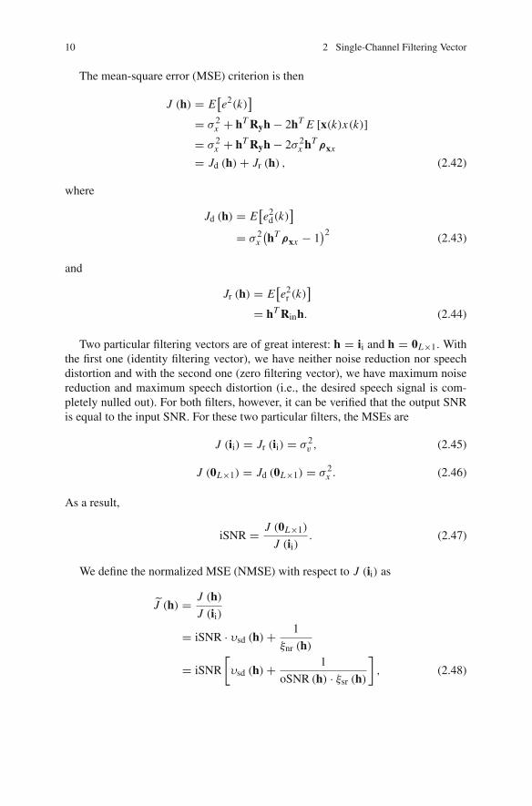
The mean-square error (MSE) criterion is then
J (h) = E[e2(k)
]
= σ 2x + hT Ryh − 2hT E [x(k)x(k)]
= σ 2x + hT Ryh − 2σ 2
x hT ρxx
= Jd (h) + Jr (h) , (2.42)
where
Jd (h) = E[e2
d(k)]
= σ 2x
(hT ρxx − 1
)2 (2.43)
and
Jr (h) = E[e2
r (k)]
= hT Rinh. (2.44)
Two particular filtering vectors are of great interest: h = ii and h = 0L×1. Withthe first one (identity filtering vector), we have neither noise reduction nor speechdistortion and with the second one (zero filtering vector), we have maximum noisereduction and maximum speech distortion (i.e., the desired speech signal is com-pletely nulled out). For both filters, however, it can be verified that the output SNRis equal to the input SNR. For these two particular filters, the MSEs are
J (ii) = Jr (ii) = σ 2v , (2.45)
J (0L×1) = Jd (0L×1) = σ 2x . (2.46)
As a result,
iSNR = J (0L×1)
J (ii). (2.47)
We define the normalized MSE (NMSE) with respect to J (ii) as
J̃ (h) = J (h)
J (ii)
= iSNR · υsd (h) + 1
ξnr (h)
= iSNR
[υsd (h) + 1
oSNR (h) · ξsr (h)
], (2.48)

2.3 Performance Measures 11
where
υsd (h) = Jd (h)
Jd (0L×1), (2.49)
iSNR · υsd (h) = Jd (h)
Jr (ii), (2.50)
ξnr (h) = Jr (ii)Jr (h)
, (2.51)
oSNR (h) · ξsr (h) = Jd (0L×1)
Jr (h). (2.52)
This shows how this NMSE and the different MSEs are related to the performancemeasures.
We define the NMSE with respect to J (0L×1) as
J (h) = J (h)
J (0L×1)
= υsd (h) + 1
oSNR (h) · ξsr (h)(2.53)
and, obviously,
J̃ (h) = iSNR · J (h) . (2.54)
We are only interested in filters for which
Jd (ii) ≤ Jd (h) < Jd (0L×1) , (2.55)
Jr (0L×1) < Jr (h) < Jr (ii) . (2.56)
From the two previous expressions, we deduce that
0 ≤ υsd (h) < 1, (2.57)
1 < ξnr (h) < ∞. (2.58)
It is clear that the objective of noise reduction is to find optimal filtering vectors thatwould either minimize J (h) or minimize Jd (h) or Jr (h) subject to some constraint.
2.4 Optimal Filtering Vectors
In this section, we are going to derive the most important filtering vectors that canhelp mitigate the level of the noise picked up by the microphone signal.

12 2 Single-Channel Filtering Vector
2.4.1 Maximum Signal-to-Noise Ratio (SNR)
The maximum SNR filter, hmax, is obtained by maximizing the output SNR as givenin (2.22) from which, we recognize the generalized Rayleigh quotient [7]. It is wellknown that this quotient is maximized with the maximum eigenvector of the matrixR−1
in Rxd . Let us denote by λmax the maximum eigenvalue corresponding to thismaximum eigenvector. Since the rank of the mentioned matrix is equal to 1, we have
λmax = tr(R−1
in Rxd
)
= σ 2x · ρT
xx R−1in ρxx , (2.59)
where tr (·) denotes the trace of a square matrix. As a result,
oSNR (hmax) = λmax
= σ 2x · ρT
xx R−1in ρxx , (2.60)
which corresponds to the maximum possible output SNR, i.e., oSNRmax.
Obviously, we also have
hmax = ςR−1in ρxx , (2.61)
where ς is an arbitrary non-zero scaling factor. While this factor has no effect onthe output SNR, it may have on the speech distortion. In fact, all filters (except forthe LCMV) derived in the rest of this section are equivalent up to this scaling factor.These filters also try to find the respective scaling factors depending on what weoptimize.
2.4.2 Wiener
The Wiener filter is easily derived by taking the gradient of the MSE, J (h)
[Eq. (2.42)], with respect to h and equating the result to zero:
hW = σ 2x R−1
y ρxx .
The Wiener filter can also be expressed as
hW = R−1y E [x(k)x(k)]
= R−1y Rxii
= (IL − R−1
y Rv)ii, (2.62)
where IL is the identity matrix of size L × L . The above formulation depends on thesecond-order statistics of the observation and noise signals. The correlation matrix

2.4 Optimal Filtering Vectors 13
Ry can be estimated from the observation signal while the other correlation matrix,Rv, can be estimated during noise-only intervals assuming that the statistics of thenoise do not change much with time.
We now propose to write the general form of the Wiener filter in another way thatwill make it easier to compare to other optimal filters. We can verify that
Ry = σ 2x ρxxρ
Txx + Rin. (2.63)
Determining the inverse of Ry from the previous expression with the Woodbury’sidentity, we get
R−1y = R−1
in − R−1in ρxxρ
Txx R−1
in
σ−2x + ρT
xx R−1in ρxx
. (2.64)
Substituting (2.64) into (2.62), leads to another interesting formulation of the Wienerfilter:
hW = σ 2x R−1
in ρxx
1 + σ 2x ρT
xx R−1in ρxx
, (2.65)
that we can rewrite as
hW = σ 2x R−1
in ρxxρTxx
1 + λmaxii
= R−1in
(Ry − Rin
)
1 + tr[R−1
in
(Ry − Rin
)] ii
= R−1in Ry − IL
1 − L + tr(R−1
in Ry) ii. (2.66)
From (2.66), we deduce that the output SNR is
oSNR (hW) = λmax
= tr(R−1
in Ry) − L . (2.67)
We observe from (2.67) that the more the amount of noise, the smaller is the outputSNR.
The speech distortion index is an explicit function of the output SNR:
υsd (hW) = 1
[1 + oSNR (hW)]2 ≤ 1. (2.68)
The higher the value of oSNR (hW) , the less the desired signal is distorted.

14 2 Single-Channel Filtering Vector
Clearly,
oSNR (hW) ≥ iSNR, (2.69)
since the Wiener filter maximizes the output SNR.It is of interest to observe that the two filters hmax and hW are equivalent up to a
scaling factor. Indeed, taking
ς = σ 2x
1 + λmax(2.70)
in (2.61) (maximum SNR filter), we find (2.66) (Wiener filter).With the Wiener filter, the noise and speech reduction factors are
ξnr (hW) = (1 + λmax)2
iSNR · λmax
≥(
1 + 1
λmax
)2
, (2.71)
ξsr (hW) =(
1 + 1
λmax
)2
. (2.72)
Finally, we give the minimum NMSEs (MNMSEs):
J̃ (hW) = iSNR
1 + oSNR (hW)≤ 1, (2.73)
J (hW) = 1
1 + oSNR (hW)≤ 1. (2.74)
2.4.3 Minimum Variance Distortionless Response(MVDR)
The celebrated minimum variance distortionless response (MVDR) filter proposedby Capon [8, 9] is usually derived in a context where we have at least two sensors (ormicrophones) available. Interestingly, with the linear model proposed in this chapter,we can also derive the MVDR (with one sensor only) by minimizing the MSE of theresidual interference-plus-noise, Jr (h) , with the constraint that the desired signal isnot distorted. Mathematically, this is equivalent to
minh
hT Rinh subject to hT ρxx = 1, (2.75)

2.4 Optimal Filtering Vectors 15
for which the solution is
hMVDR = R−1in ρxx
ρTxx R−1
in ρxx
, (2.76)
that we can rewrite as
hMVDR = R−1in Ry − IL
tr(R−1
in Ry) − L
ii
= σ 2x R−1
in ρxx
λmax. (2.77)
Alternatively, we can express the MVDR as
hMVDR = R−1y ρxx
ρTxx R−1
y ρxx
. (2.78)
The Wiener and MVDR filters are simply related as follows:
hW = ς0hMVDR, (2.79)
where
ς0 = hTWρxx
= λmax
1 + λmax. (2.80)
So, the two filters hW and hMVDR are equivalent up to a scaling factor. From atheoretical point of view, this scaling is not significant. But from a practical pointof view it can be important. Indeed, the signals are usually nonstationary and theestimations are done frame by frame, so it is essential to have this scaling factorright from one frame to another in order to avoid large distortions. Therefore, itis recommended to use the MVDR filter rather than the Wiener filter in speechenhancement applications.
It is clear that we always have
oSNR (hMVDR) = oSNR (hW) , (2.81)
υsd (hMVDR) = 0, (2.82)
ξsr (hMVDR) = 1, (2.83)
ξnr (hMVDR) = oSNR (hMVDR)
iSNR≤ ξnr (hW) , (2.84)

16 2 Single-Channel Filtering Vector
and
1 ≥ J̃ (hMVDR) = iSNR
oSNR (hMVDR)≥ J̃ (hW) , (2.85)
J (hMVDR) = 1
oSNR (hMVDR)≥ J (hW) . (2.86)
2.4.4 Prediction
Assume that we can find a simple prediction filter g of length L in such a way that
x(k) ≈ x(k)g. (2.87)
In this case, we can derive a distortionless filter for noise reduction as follows:
minh
hT Ryh subject to hT g = 1. (2.88)
We deduce the solution
hP = R−1y g
gT R−1y g
. (2.89)
Now, we can find the optimal g in the Wiener sense. For that, we need to definethe error signal vector
eP(k) = x(k) − x(k)g (2.90)
and form the MSE
J (g) = E[eT
P (k)eP(k)]. (2.91)
By minimizing J (g) with respect to g, we easily find the optimal filter
go = ρxx . (2.92)
It is interesting to observe that the error signal vector with the optimal filter, go,
corresponds to the interference signal, i.e.,
eP,o(k) = x(k) − x(k)ρxx
= xi(k). (2.93)
This result is obviously expected because of the orthogonality principle.

2.4 Optimal Filtering Vectors 17
Substituting (2.92) into (2.89), we find that
hP = R−1y ρxx
ρTxx R−1
y ρxx
. (2.94)
Clearly, the two filters hMVDR and hP are identical. Therefore, the prediction approachcan be seen as another way to derive the MVDR. This approach is also an intuitivemanner to justify the decomposition given in (2.5).
Left multiplying both sides of (2.93) by hTP results in
x(k) = hTP x(k) − hT
P eP,o(k). (2.95)
Therefore, the filter hP can also be interpreted as a temporal prediction filter that isless noisy than the one that can be obtained from the noisy signal, y(k), directly.
2.4.5 Tradeoff
In the tradeoff approach, we try to compromise between noise reduction and speechdistortion. Instead of minimizing the MSE to find the Wiener filter or minimizing thefilter output with a distortionless constraint to find the MVDR as we already did inthe preceding subsections, we could minimize the speech distortion index with theconstraint that the noise reduction factor is equal to a positive value that is greaterthan 1. Mathematically, this is equivalent to
minh
Jd (h) subject to Jr (h) = βσ 2v , (2.96)
where 0 < β < 1 to insure that we get some noise reduction. By using a Lagrangemultiplier, μ > 0, to adjoin the constraint to the cost function and assuming that thematrix Rxd + μRin is invertible, we easily deduce the tradeoff filter
hT,μ = σ 2x
[Rxd + μRin
]−1ρxx
= R−1in ρxx
μσ−2x + ρT
xx R−1in ρxx
= R−1in Ry − IL
μ − L + tr(R−1
in Ry) ii, (2.97)
where the Lagrange multiplier, μ, satisfies
Jr(hT,μ
) = βσ 2v . (2.98)
However, in practice it is not easy to determine the optimal μ. Therefore, when thisparameter is chosen in an ad hoc way, we can see that for

18 2 Single-Channel Filtering Vector
• μ = 1, hT,1 = hW, which is the Wiener filter;• μ = 0, hT,0 = hMVDR, which is the MVDR filter;• μ > 1, results in a filter with low residual noise (compared with the Wiener filter)
at the expense of high speech distortion;• μ < 1, results in a filter with high residual noise and low speech distortion.
Note that the MVDR cannot be derived from the first line of (2.97) since by takingμ = 0, we have to invert a matrix that is not full rank.
Again, we observe here as well that the tradeoff, Wiener, and maximum SNRfilters are equivalent up to a scaling factor. As a result, the output SNR of the tradeofffilter is independent of μ and is identical to the output SNR of the Wiener filter, i.e.,
oSNR(hT,μ
) = oSNR (hW) , ∀μ ≥ 0. (2.99)
We have
υsd(hT,μ
) =(
μ
μ + λmax
)2
, (2.100)
ξsr(hT,μ
) =(
1 + μ
λmax
)2
, (2.101)
ξnr(hT,μ
) = (μ + λmax)2
iSNR · λmax, (2.102)
and
J̃(hT,μ
) = iSNRμ2 + λmax
(μ + λmax)2 ≥ J (hW) , (2.103)
J(hT,μ
) = μ2 + λmax
(μ + λmax)2 ≥ J (hW) . (2.104)
2.4.6 Linearly Constrained Minimum Variance(LCMV)
We can derive a linearly constrained minimum variance (LCMV) filter [10, 11],which can handle more than one linear constraint, by exploiting the structure of thenoise signal.
In Sect. 2.1, we decomposed the vector x(k) into two orthogonal components toextract the desired signal, x(k). We can also decompose (but for a different objectiveas explained below) the noise signal vector, v(k), into two orthogonal vectors:

2.4 Optimal Filtering Vectors 19
v(k) = ρvv · v(k) + vu(k), (2.105)
where ρvv is defined in a similar way to ρxx and vu(k) is the noise signal vector thatis uncorrelated with v(k).
Our problem this time is the following. We wish to perfectly recover our desiredsignal, x(k), and completely remove the correlated components of the noise signal,ρvv · v(k). Thus, the two constraints can be put together in a matrix form as
CTxvh =
[10
], (2.106)
where
Cxv = [ρxx ρvv
](2.107)
is our constraint matrix of size L × 2. Then, our optimal filter is obtained by min-imizing the energy at the filter output, with the constraints that the correlated noisecomponents are cancelled and the desired speech is preserved, i.e.,
hLCMV = arg minh
hT Ryh subject to CTxvh =
[10
]. (2.108)
The solution to (2.108) is given by
hLCMV = R−1y Cxv
(CT
xvR−1y Cxv
)−1[
10
]. (2.109)
By developing (2.109), it can easily be shown that the LCMV can be written as afunction of the MVDR:
hLCMV = 1
1 − γ 2 hMVDR − γ 2
1 − γ 2 t, (2.110)
where
γ 2 =(ρT
xx R−1y ρvv
)2
(ρT
xx R−1y ρxx
)(ρT
vvR−1y ρvv
) , (2.111)
with 0 ≤ γ 2 ≤ 1, hMVDR is defined in (2.78), and
t = R−1y ρvv
ρTxx R−1
y ρvv
. (2.112)
We observe from (2.110) that when γ 2 = 0, the LCMV filter becomes the MVDRfilter; however, when γ 2 tends to 1, which happens if and only if ρxx = ρvv, wehave no solution since we have conflicting requirements.

20 2 Single-Channel Filtering Vector
Obviously, we always have
oSNR (hLCMV) ≤ oSNR (hMVDR) , (2.113)
υsd (hLCMV) = 0, (2.114)
ξsr (hLCMV) = 1, (2.115)
and
ξnr (hLCMV) ≤ ξnr (hMVDR) ≤ ξnr (hW) . (2.116)
The LCMV filter is able to remove all the correlated noise; however, its overall noisereduction is lower than that of the MVDR filter.
2.4.7 Practical Considerations
All the algorithms presented in the preceding subsections can be implemented fromthe second-order statistics estimates of the noise and noisy signals. Let us take theMVDR as an example. In this filter, we need the estimates of Ry and ρxx . Thecorrelation matrix, Ry, can be easily estimated from the observations. However, thecorrelation vector, ρxx , cannot be estimated directly since x(k) is not accessible butit can be rewritten as
ρxx = E[y(k)y(k)
] − E [v(k)v(k)]
σ 2y − σ 2
v
= σ 2y ρyy − σ 2
v ρvv
σ 2y − σ 2
v
, (2.117)
which now depends on the statistics of y(k) and v(k). However, a voice activitydetector (VAD) is required in order to be able to estimate the statistics of the noisesignal during silences [i.e., when x(k) = 0 ]. Nowadays, more and more sophisticatedVADs are developed [12] since a VAD is an integral part of most speech enhancementalgorithms. A good VAD will obviously improve the performance of a noise reductionfilter since the estimates of the signals statistics will be more reliable. A systemintegrating an optimal filter and a VAD may not be easy to design but much progresshas been made recently in this area of research [13].
2.5 Summary
In this chapter, we revisited the single-channel noise reduction problem in the timedomain. We showed how to extract the desired signal sample from a vector containing

2.5 Summary 21
its past samples. Thanks to the orthogonal decomposition that results from this, thepresentation of the problem is simplified. We defined several interesting performancemeasures in this context and deduced optimal noise reduction filters: maximumSNR, Wiener, MVDR, prediction, tradeoff, and LCMV. Interestingly, all these filters(except for the LCMV) are equivalent up to a scaling factor. Consequently, theirperformance in terms of SNR improvement is the same given the same statisticsestimates.
References
1. J. Benesty, J. Chen, Y. Huang, I. Cohen, Noise Reduction in Speech Processing (Springer,Berlin, 2009)
2. P. Vary, R. Martin, Digital Speech Transmission: Enhancement, Coding and Error Concealment(Wiley, Chichester, 2006)
3. P. Loizou, Speech Enhancement: Theory and Practice (CRC Press, Boca Raton, 2007)4. J. Benesty, J. Chen, Y. Huang, S. Doclo, Study of the Wiener filter for noise reduction, in Speech
Enhancement, Chap. 2, ed. by J. Benesty, S. Makino, J. Chen (Springer, Berlin, 2005)5. J. Chen, J. Benesty, Y. Huang, S. Doclo, New insights into the noise reduction Wiener filter.
IEEE Trans. Audio Speech Language Process. 14, 1218–1234 (2006)6. S. Haykin, Adaptive Filter Theory, 4th edn. (Prentice-Hall, Upper Saddle River, 2002)7. J.N. Franklin, Matrix Theory (Prentice-Hall, Englewood Cliffs, 1968)8. J. Capon, High resolution frequency-wavenumber spectrum analysis. Proc. IEEE 57, 1408–
1418 (1969)9. R.T. Lacoss, Data adaptive spectral analysis methods. Geophysics 36, 661–675 (1971)
10. O. Frost, An algorithm for linearly constrained adaptive array processing. Proc. IEEE 60,926–935 (1972)
11. M. Er, A. Cantoni, Derivative constraints for broad-band element space antenna array proces-sors. IEEE Trans. Acoust. Speech Signal Process. 31, 1378–1393 (1983)
12. I. Cohen, Noise spectrum estimation in adverse environments: improved minima controlledrecursive averaging. IEEE Trans. Speech Audio Process. 11, 466–475 (2003)
13. I. Cohen, J. Benesty, S. Gannot (eds.), Speech Processing in Modern Communication—Challenges and Perspectives (Springer, Berlin, 2010)


Chapter 3Single-Channel Noise Reduction witha Rectangular Filtering Matrix
In the previous chapter, we tried to estimate one sample only at a time from theobservation signal vector. In this part, we are going to estimate more than one sampleat a time. As a result, we now deal with a rectangular filtering matrix instead of afiltering vector. If M is the number of samples to be estimated and L is the lengthof the observation signal vector, then the size of the filtering matrix is M × L . Also,this approach is more general and all the results from Chap. 2 are particular casesof the results derived in this chapter by just setting M = 1. The signal model is thesame as in Sect. 2.1; so we start by explaining the principle of linear filtering with arectangular matrix.
3.1 Linear Filtering with a Rectangular Matrix
Define the vector of length M:
xM (k) = [x(k) x(k − 1) · · · x(k − M + 1)]T , (3.1)
where M ≤ L . In the general linear filtering approach, we estimate the desired signalvector, xM (k), by applying a linear transformation to y(k) [1–4], i.e.,
zM (k) = Hy(k)
= H [x(k) + v(k)]
= xMf (k) + vM
rn (k), (3.2)
where zM (k) is the estimate of xM (k),
H =
⎡
⎢⎢⎢⎣
hT1
hT2...
hTM
⎤
⎥⎥⎥⎦
(3.3)
J. Benesty and J. Chen, Optimal Time-Domain Noise Reduction Filters, 23SpringerBriefs in Electrical and Computer Engineering, 1,DOI: 10.1007/978-3-642-19601-0_3, © Jacob Benesty 2011
24 3 Single-Channel Filtering Matrix
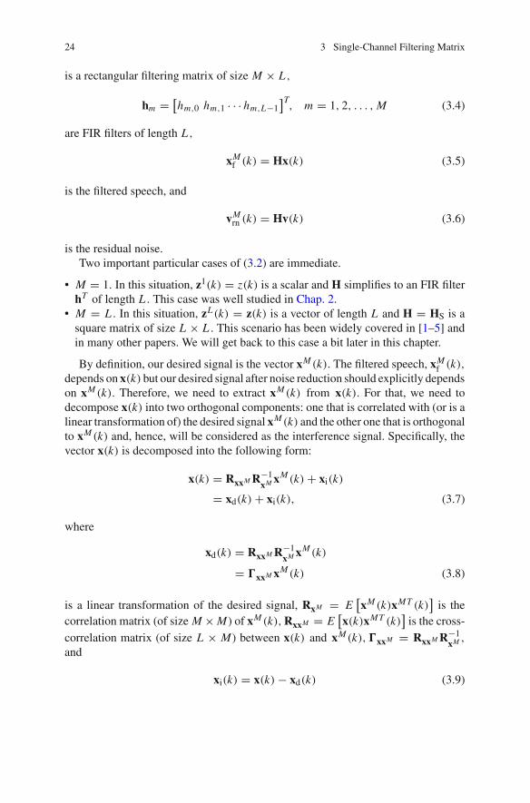
is a rectangular filtering matrix of size M × L ,
hm = [hm,0 hm,1 · · · hm,L−1
]T, m = 1, 2, . . . , M (3.4)
are FIR filters of length L ,
xMf (k) = Hx(k) (3.5)
is the filtered speech, and
vMrn (k) = Hv(k) (3.6)
is the residual noise.Two important particular cases of (3.2) are immediate.
• M = 1. In this situation, z1(k) = z(k) is a scalar and H simplifies to an FIR filterhT of length L . This case was well studied in Chap. 2.
• M = L . In this situation, zL(k) = z(k) is a vector of length L and H = HS is asquare matrix of size L × L . This scenario has been widely covered in [1–5] andin many other papers. We will get back to this case a bit later in this chapter.
By definition, our desired signal is the vector xM (k). The filtered speech, xMf (k),
depends on x(k) but our desired signal after noise reduction should explicitly dependson xM (k). Therefore, we need to extract xM(k) from x(k). For that, we need todecompose x(k) into two orthogonal components: one that is correlated with (or is alinear transformation of) the desired signal xM(k) and the other one that is orthogonalto xM (k) and, hence, will be considered as the interference signal. Specifically, thevector x(k) is decomposed into the following form:
x(k) = RxxM R−1xM xM (k) + xi(k)
= xd(k) + xi(k), (3.7)
where
xd(k) = RxxM R−1xM xM (k)
= �xxM xM (k) (3.8)
is a linear transformation of the desired signal, RxM = E[xM (k)xMT (k)
]is the
correlation matrix (of size M × M) of xM (k), RxxM = E[x(k)xMT (k)
]is the cross-
correlation matrix (of size L × M) between x(k) and xM(k),�xxM = RxxM R−1xM ,
and
xi(k) = x(k) − xd(k) (3.9)

3.1 Linear Filtering with a Rectangular Matrix 25
is the interference signal. It is easy to see that xd(k) and xi(k) are orthogonal, i.e.,
E[xd(k)xT
i (k)] = 0L×L . (3.10)
For the particular case M = L , we have �xx = IL , which is the identity matrix(of size L × L), and xd(k) coincides with x(k), which obviously makes sense. ForM = 1,�xx1 simplifies to the normalized correlation vector (see Chap. 2)
ρxx = E [x(k)x(k)]
E[x2(k)
] . (3.11)
Substituting (3.7) into (3.2), we get
zM(k) = H [xd(k) + xi(k) + v(k)]
= xMfd (k) + xM
ri (k) + vMrn (k), (3.12)
where
xMfd (k) = Hxd(k) (3.13)
is the filtered desired signal,
xMri (k) = Hxi(k) (3.14)
is the residual interference, and vMrn (k) = Hv(k), again, represents the residual
noise. It can be checked that the three terms xMfd (k), xM
ri (k), and vMrn (k) are mutually
orthogonal. Therefore, the correlation matrix of zM(k) is
RzM = E[zM (k)zMT (k)
]
= RxMfd
+ RxMri
+ RvMrn
, (3.15)
where
RxMfd
= HRxd HT , (3.16)
RxMri
= HRxi HT
= HRxHT − HRxd HT , (3.17)
RvMrn
= HRvHT , (3.18)
Rxd = �xxM RxM �TxxM is the correlation matrix (whose rank is equal to M) of xd(k),
and Rxi = E[xi(k)xT
i (k)]
is the correlation matrix of xi(k). The correlation matrixof zM (k) is helpful in defining meaningful performance measures.

26 3 Single-Channel Filtering Matrix
3.2 Joint Diagonalization
By exploiting the decomposition of x(k), we can decompose the correlation matrixof y(k) as
Ry = Rxd + Rin
= �xxM RxM �TxxM + Rin, (3.19)
where
Rin = Rxi + Rv (3.20)
is the interference-plus-noise correlation matrix. It is interesting to observe from(3.19) that the noisy signal correlation matrix is the sum of two other correlationmatrices: the linear transformation of the desired signal correlation matrix of rankM and the interference-plus-noise correlation matrix of rank L .
The two symmetric matrices Rxd and Rin can be jointly diagonalized as follows[6, 7]:
BT Rxd B = �, (3.21)
BT RinB = IL , (3.22)
where B is a full-rank square matrix (of size L × L) and � is a diagonal matrix whosemain elements are real and nonnegative. Furthermore, � and B are the eigenvalueand eigenvector matrices, respectively, of R−1
in Rxd , i.e.,
R−1in Rxd B = B�. (3.23)
Since the rank of the matrix Rxd is equal to M, the eigenvalues of R−1in Rxd can
be ordered as λM1 ≥ λM
2 ≥ · · · ≥ λMM > λM
M+1 = · · · = λML = 0. In other
words, the last L − M eigenvalues of R−1in Rxd are exactly zero while its first M
eigenvalues are positive, with λM1 being the maximum eigenvalue. We also denote
by bM1 , bM
2 , . . . , bMM , bM
M+1, . . . , bML , the corresponding eigenvectors. Therefore, the
noisy signal covariance matrix can also be diagonalized as
BT RyB = � + IL . (3.24)
Note that the same diagonalization was proposed in [8] but for the classical subspaceapproach [2].
Now, we have all the necessary ingredients to define the performance measuresand derive the most well-known optimal filtering matrices.

3.3 Performance Measures 27
3.3 Performance Measures
In this section, the performance measures tailored for linear filtering with a rectan-gular matrix are defined.
3.3.1 Noise Reduction
The input SNR was already defined in Chap. 2; but it can be rewritten as
iSNR = σ 2x
σ 2v
= tr (Rx)
tr (Rv). (3.25)
Taking the trace of the filtered desired signal correlation matrix from the right-hand side of (3.15) over the trace of the two other correlation matrices gives theoutput SNR:
oSNR (H) =tr
(RxM
fd
)
tr(
RxMri
+ RvMrn
)
= tr(H�xxM RxM �T
xxM HT)
tr(HRinHT
) . (3.26)
The obvious objective is to find an appropriate H in such a way that oSNR (H) ≥iSNR.
For the particular filtering matrix
H = Ii = [IM 0M×(L−M)
], (3.27)
called the identity filtering matrix, where IM is the M × M identity matrix, we have
oSNR (Ii) = iSNR. (3.28)
With Ii, the SNR cannot be improved.The maximum output SNR cannot be derived from a simple inequality as it was
done in the previous chapter in the particular case of M = 1. We will see how to findthis value when we derive the maximum SNR filter.
The noise reduction factor is
ξnr (H) = M · σ 2v
tr(
RxMri
+ RvMrn
)
= M · σ 2v
tr(HRinHT
) . (3.29)
Any good choice of H should lead to ξnr (H) ≥ 1.

28 3 Single-Channel Filtering Matrix
3.3.2 Speech Distortion
The desired speech signal can be distorted by the rectangular filtering matrix. There-fore, the speech reduction factor is defined as
ξsr (H) = M · σ 2x
tr(
RxMfd
)
= M · σ 2x
tr(H�xxM RxM �T
xxM HT) . (3.30)
A rectangular filtering matrix that does not affect the desired signal requires theconstraint
H�xxM = IM . (3.31)
Hence, ξsr (H) = 1 in the absence of distortion and ξsr (H) > 1 in the presence ofdistortion.
By making the appropriate substitutions, one can derive the relationship amongthe measures defined so far:
oSNR (H)
iSNR= ξnr (H)
ξsr (H). (3.32)
When no distortion occurs, the gain in SNR coincides with the noise reduction factor.We can also quantify the distortion with the speech distortion index:
υsd (H) = 1
M·
E{[
xMfd (k) − xM(k)
]T [xM
fd (k) − xM(k)]}
σ 2x
= 1
M·
tr[(
H�xxM − IM)
RxM
(H�xxM − IM
)T]
σ 2x
. (3.33)
The speech distortion index is always greater than or equal to 0 and should be upperbounded by 1 for optimal filtering matrices; so the higher is the value of υsd (H) ,
the more the desired signal is distorted.
3.3.3 MSE Criterion
Since the desired signal is a vector of length M, so is the error signal. We define theerror signal vector between the estimated and desired signals as
eM(k) = zM(k) − xM (k)
= Hy(k) − xM (k),(3.34)

3.3 Performance Measures 29
which can also be expressed as the sum of two orthogonal error signal vectors:
eM (k) = eMd (k) + eM
r (k), (3.35)
where
eMd (k) = xM
fd (k) − xM (k)
= (H�xxM − IM
)xM (k) (3.36)
is the signal distortion due to the rectangular filtering matrix and
eMr (k) = xM
ri (k) + vMrn (k)
= Hxi(k) + Hv(k) (3.37)
represents the residual interference-plus-noise.Having defined the error signal, we can now write the MSE criterion:
J (H) = 1
M· tr
{E
[eM (k)eMT (k)
]}(3.38)
= 1
M
[tr(RxM
) + tr(HRyHT ) − 2tr
(HRyxM
) ]
= 1
M
[tr
(RxM
) + tr(HRyHT ) − 2tr
(H�xxM RxM
) ],
where
RyxM = E[y(k)xMT (k)
]
= �xxM RxM
is the cross-correlation matrix between y(k) and xM (k).
Using the fact that E[eM
d (k)eMTr (k)
] = 0M×M , J (H) can be expressed as thesum of two other MSEs, i.e.,
J (H) = 1
M· tr
{E
[eM
d (k)eMTd (k)
]} + 1
M· tr
{E
[eM
r (k)eMTr (k)
]}
= Jd (H) + Jr (H) . (3.39)
Two particular filtering matrices are of great importance: H = Ii and H = 0M×L .
With the first one (identity filtering matrix), we have neither noise reduction norspeech distortion and with the second one (zero filtering matrix), we have maximumnoise reduction and maximum speech distortion (i.e., the desired speech signal iscompletely nulled out). For both filtering matrices, however, it can be verified that

30 3 Single-Channel Filtering Matrix
the output SNR is equal to the input SNR. For these two particular filtering matrices,the MSEs are
J (Ii) = Jr (Ii) = σ 2v , (3.40)
J (0M×L) = Jd (0M×L) = σ 2x . (3.41)
As a result,
iSNR = J (0M×L)
J (Ii). (3.42)
We define the NMSE with respect to J (Ii) as
J̃ (H) = J (H)
J (Ii)
= iSNR · υsd (H) + 1
ξnr (H)
= iSNR
[υsd (H) + 1
oSNR (H) · ξsr (H)
], (3.43)
where
υsd (H) = Jd (H)
Jd (0M×L), (3.44)
iSNR · υsd (H) = Jd (H)
Jr (Ii), (3.45)
ξnr (H) = Jr (Ii)
Jr (H), (3.46)
oSNR (H) · ξsr (H) = Jd (0M×L)
Jr (H). (3.47)
This shows how this NMSE and the different MSEs are related to the performancemeasures.
We define the NMSE with respect to J (0M×L) as
J (H) = J (H)
J (0M×L)
= υsd (H) + 1
oSNR (H) · ξsr (H)(3.48)
and, obviously,
J̃ (H) = iSNR · J (H) . (3.49)

3.3 Performance Measures 31
We are only interested in filtering matrices for which
Jd (Ii) ≤ Jd (H) < Jd (0M×L) , (3.50)
Jr (0M×L) < Jr (H) < Jr (Ii) . (3.51)
From the two previous expressions, we deduce that
0 ≤ υsd (H) < 1, (3.52)
1 < ξnr (H) < ∞. (3.53)
The optimal filtering matrices are obtained by minimizing J (H) or minimizingJr (H) or Jd (H) subject to some constraint.
3.4 Optimal Rectangular Filtering Matrices
In this section, we are going to derive the most important filtering matrices that canhelp reduce the noise picked up by the microphone signal.
3.4.1 Maximum SNR
Our first optimal filtering matrix is not derived from the MSE criterion but from theoutput SNR defined in (3.26) that we can rewrite as
oSNR (H) =∑M
m=1 hTmRxd hm
∑Mm=1 hT
mRinhm. (3.54)
It is then natural to try to maximize this SNR with respect to H. Let us first give thefollowing lemma.
Lemma 3.1 We have
oSNR (H) ≤ maxm
hTmRxd hm
hTmRinhm
= χ. (3.55)
Proof Let us define the positive reals am = hTmRxd hm and bm = hT
mRinhm . Wehave
∑Mm=1 am
∑Mm=1 bm
=M∑
m=1
(am
bm· bm∑M
i=1 bi
)
. (3.56)

32 3 Single-Channel Filtering Matrix
Now, define the following two vectors:
u =[
a1
b1
a2
b2· · · aM
bM
]T
, (3.57)
u′ =[
b1∑M
i=1 bi
b2∑M
i=1 bi· · · bM
∑Mi=1 bi
]T
. (3.58)
Using the Holder’s inequality, we see that∑M
m=1 am∑M
m=1 bm= uT u′
≤ ‖u‖∞∥∥u′∥∥
1 = maxm
am
bm, (3.59)
which ends the proof. ��Theorem 3.1 The maximum SNR filtering matrix is given by
Hmax =
⎡
⎢⎢⎢⎣
β1bMT1
β2bMT1...
βmbMT1
⎤
⎥⎥⎥⎦
, (3.60)
where βm, m = 1, 2, . . . , M are real numbers with at least one of them differentfrom 0. The corresponding output SNR is
oSNR (Hmax) = λM1 . (3.61)
We recall that λM1 is the maximum eigenvalue of the matrix R−1
in Rxd and its corre-sponding eigenvector is bM
1 .
Proof From Lemma 3.1, we know that the output SNR is upper bounded by χ whosemaximum value is clearly λM
1 . On the other hand, it can be checked from (3.54)that oSNR (Hmax) = λM
1 . Since this output SNR is maximal, Hmax is indeed themaximum SNR filtering matrix. ��Property 3.1 The output SNR with the maximum SNR filtering matrix is alwaysgreater than or equal to the input SNR, i.e., oSNR (Hmax) ≥ iSNR.
It is interesting to see that we have these bounds:
0 ≤ oSNR (H) ≤ λM1 ,∀H, (3.62)
but, obviously, we are only interested in filtering matrices that can improve the outputSNR, i.e., oSNR (H) ≥ iSNR.
For a fixed L , increasing the value of M (from 1 to L) will, in principle, increase theoutput SNR of the maximum SNR filtering matrix since more and more information istaken into account. The distortion should also increase significantly as M is increased.

3.4 Optimal Rectangular Filtering Matrices 33
3.4.2 Wiener
If we differentiate the MSE criterion, J (H) , with respect to H and equate the resultto zero, we find the Wiener filtering matrix
HW = RxM �TxxM R−1
y
= IiRxR−1y
= Ii(IL − RvR−1
y). (3.63)
This matrix depends only on the second-order statistics of the noise and observationsignals. Note that the first line of HW is exactly hT
W.
Lemma 3.2 We can rewrite the Wiener filtering matrix as
HW = (IM + RxM �T
xxM R−1in �xxM
)−1RxM �TxxM R−1
in
= (R−1
xM + �TxxM R−1
in �xxM
)−1�T
xxM R−1in . (3.64)
Proof This expression is easy to show by applying the Woodbury’s identity in (3.19)and then substituting the result in (3.63). ��
The form of the Wiener filtering matrix presented in (3.64) is interesting becauseit shows an obvious link with some other optimal filtering matrices as it will beverified later.
Another way to express Wiener is
HW = Ii�xxM RxM �TxxM R−1
y
= Ii(IL − RinR−1
y). (3.65)
Using the joint diagonalization, we can rewrite Wiener as a subspace-type approach:
HW = IiB−T � (� + IL)−1 BT
= IiB−T[
� 0M×(L−M)
0(L−M)×M 0(L−M)×(L−M)
]BT
= T[
� 0M×(L−M)
0(L−M)×M 0(L−M)×(L−M)
]BT , (3.66)
where
T =
⎡
⎢⎢⎢⎣
tT1
tT2...
tTM
⎤
⎥⎥⎥⎦
= IiB−T (3.67)
34 3 Single-Channel Filtering Matrix
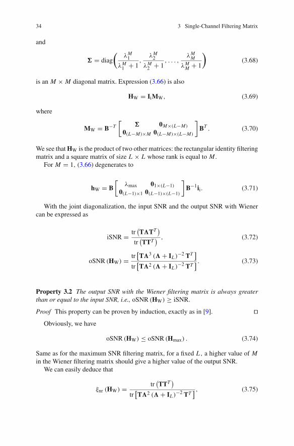
and
� = diag
(λM
1
λM1 + 1
,λM
2
λM2 + 1
, . . . ,λM
M
λMM + 1
)(3.68)
is an M × M diagonal matrix. Expression (3.66) is also
HW = IiMW, (3.69)
where
MW = B−T[
� 0M×(L−M)
0(L−M)×M 0(L−M)×(L−M)
]BT . (3.70)
We see that HW is the product of two other matrices: the rectangular identity filteringmatrix and a square matrix of size L × L whose rank is equal to M.
For M = 1, (3.66) degenerates to
hW = B[
λmax 01×(L−1)
0(L−1)×1 0(L−1)×(L−1)
]B−1ii. (3.71)
With the joint diagonalization, the input SNR and the output SNR with Wienercan be expressed as
iSNR = tr(T�TT
)
tr(TTT
) , (3.72)
oSNR (HW) = tr[T�3 (� + IL)−2 TT
]
tr[T�2 (� + IL)−2 TT
] . (3.73)
Property 3.2 The output SNR with the Wiener filtering matrix is always greaterthan or equal to the input SNR, i.e., oSNR (HW) ≥ iSNR.
Proof This property can be proven by induction, exactly as in [9]. ��Obviously, we have
oSNR (HW) ≤ oSNR (Hmax) . (3.74)
Same as for the maximum SNR filtering matrix, for a fixed L , a higher value of Min the Wiener filtering matrix should give a higher value of the output SNR.
We can easily deduce that
ξnr (HW) = tr(TTT
)
tr[T�2 (� + IL)−2 TT
] , (3.75)

3.4 Optimal Rectangular Filtering Matrices 35
ξsr (HW) = tr(T�TT
)
tr[T�3 (� + IL)−2 TT
] , (3.76)
υsd (HW) =tr
[T� (� + IL)−1 TT R−1
xM T� (� + IL)−1 TT]
tr(T�TT
) . (3.77)
3.4.3 MVDR
We recall that the MVDR approach requires no distortion to the desired signal.Therefore, the corresponding rectangular filtering matrix is obtained by minimizingthe MSE of the residual interference-plus-noise, Jr (H) , with the constraint that thedesired signal is not distorted. Mathematically, this is equivalent to
minH
1
M· tr
(HRinHT )
subject to H�xxM = IM . (3.78)
The solution to the above optimization problem is
HMVDR = (�T
xxM R−1in �xxM
)−1�T
xxM R−1in , (3.79)
which is interesting to compare to HW (Eq. 3.64).Obviously, with the MVDR filtering matrix, we have no distortion, i.e.,
ξsr (HMVDR) = 1, (3.80)
υsd (HMVDR) = 0. (3.81)
Lemma 3.3 We can rewrite the MVDR filtering matrix as
HMVDR = (�T
xxM R−1y �xxM
)−1�T
xxM R−1y . (3.82)
Proof This expression is easy to show by using the Woodbury’s identity in R−1y . ��
From (3.82), we deduce the relationship between the MVDR and Wiener filteringmatrices:
HMVDR = (HW�xxM
)−1 HW. (3.83)
Property 3.3 The output SNR with the MVDR filtering matrix is always greater thanor equal to the input SNR, i.e., oSNR (HMVDR) ≥ iSNR.
Proof We can prove this property by induction. ��

36 3 Single-Channel Filtering Matrix
We should have
oSNR (HMVDR) ≤ oSNR (HW) ≤ oSNR (Hmax) . (3.84)
Contrary to Hmax and HW, for a fixed L , a higher value of M in the MVDR filteringmatrix implies a lower value of the output SNR.
3.4.4 Prediction
Let G be a temporal prediction matrix of size M × L so that
x(k) ≈ GT xM (k). (3.85)
The distortionless filtering matrix for noise reduction is derived by
minH
tr(HRyHT )
subject to HGT = IM , (3.86)
from which we deduce the solution
HP = (GR−1
y GT )−1GR−1y . (3.87)
The best way to find G is in the Wiener sense. Indeed, define the error signalvector
eP(k) = x(k) − GT xM(k) (3.88)
and form the MSE
J (G) = E[eT
P (k)eP(k)]. (3.89)
The minimization of J (G) with respect to G leads to
Go = �TxxM (3.90)
and substituting this result into (3.87) gives
HP = (�T
xxM R−1y �xxM
)−1�T
xxM R−1y , (3.91)
which corresponds to the MVDR.It is interesting to observe that the error signal vector with the optimal matrix,
Go, corresponds to the interference signal vector, i.e.,
eP,o(k) = x(k) − �xxM xM (k)
= xi(k). (3.92)
This result is a consequence of the orthogonality principle.

3.4 Optimal Rectangular Filtering Matrices 37
3.4.5 Tradeoff
In the tradeoff approach, we minimize the speech distortion index with the constraintthat the noise reduction factor is equal to a positive value that is greater than 1.Mathematically, this is equivalent to
minH
Jd (H) subject to Jr (H) = β Jr (Ii) , (3.93)
where 0 < β < 1 to insure that we get some noise reduction. By using a Lagrangemultiplier, μ > 0, to adjoin the constraint to the cost function and assuming that thematrix �xxM RxM �T
xxM + μRin is invertible, we easily deduce the tradeoff filteringmatrix
HT,μ = RxM �TxxM
(�xxM RxM �T
xxM + μRin)−1
, (3.94)
which can be rewritten, thanks to the Woodbury’s identity, as
HT,μ = (μR−1
xM + �TxxM R−1
in �xxM
)−1�T
xxM R−1in , (3.95)
where μ satisfies Jr(HT,μ
) = β Jr (Ii) . Usually, μ is chosen in an ad-hoc way, sothat for
• μ = 1, HT,1 = HW, which is the Wiener filtering matrix;• μ = 0 [from (3.95)], HT,0 = HMVDR, which is the MVDR filtering matrix;• μ > 1, results in a filter with low residual noise (compared with the Wiener filter)
at the expense of high speech distortion;• μ < 1, results in a filter with high residual noise and low speech distortion.
Property 3.4 The output SNR with the tradeoff filtering matrix is always greaterthan or equal to the input SNR, i.e., oSNR
(HT,μ
) ≥ iSNR, ∀μ ≥ 0.
Proof We can prove this property by induction. ��We should have for μ ≥ 1,
oSNR (HMVDR) ≤ oSNR (HW) ≤ oSNR(HT,μ
) ≤ oSNR (Hmax) (3.96)
and for μ ≤ 1,
oSNR (HMVDR) ≤ oSNR(HT,μ
) ≤ oSNR (HW) ≤ oSNR (Hmax) . (3.97)
We can write the tradeoff filtering matrix as a subspace-type approach. Indeed,from (3.94), we get
HT,μ = T[
�μ 0M×(L−M)
0(L−M)×M 0(L−M)×(L−M)
]BT , (3.98)
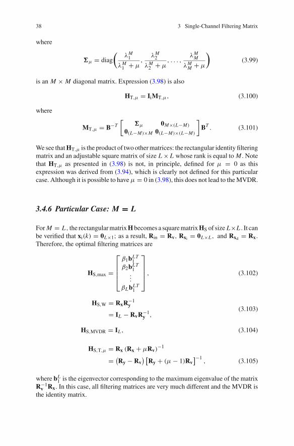
38 3 Single-Channel Filtering Matrix
where
�μ = diag
(λM
1
λM1 + μ
,λM
2
λM2 + μ
, . . . ,λM
M
λMM + μ
)(3.99)
is an M × M diagonal matrix. Expression (3.98) is also
HT,μ = IiMT,μ, (3.100)
where
MT,μ = B−T[
�μ 0M×(L−M)
0(L−M)×M 0(L−M)×(L−M)
]BT . (3.101)
We see that HT,μ is the product of two other matrices: the rectangular identity filteringmatrix and an adjustable square matrix of size L × L whose rank is equal to M. Notethat HT,μ as presented in (3.98) is not, in principle, defined for μ = 0 as thisexpression was derived from (3.94), which is clearly not defined for this particularcase. Although it is possible to have μ = 0 in (3.98), this does not lead to the MVDR.
3.4.6 Particular Case: M = L
For M = L , the rectangular matrix H becomes a square matrix HS of size L×L . It canbe verified that xi(k) = 0L×1; as a result, Rin = Rv, Rxi = 0L×L , and Rxd = Rx.
Therefore, the optimal filtering matrices are
HS,max =
⎡
⎢⎢⎢⎣
β1bLT1
β2bLT1
...
βLbLT1
⎤
⎥⎥⎥⎦
, (3.102)
HS,W = RxR−1y
= IL − RvR−1y ,
(3.103)
HS,MVDR = IL , (3.104)
HS,T,μ = Rx (Rx + μRv)−1
= (Ry − Rv
) [Ry + (μ − 1)Rv
]−1, (3.105)
where bL1 is the eigenvector corresponding to the maximum eigenvalue of the matrix
R−1v Rx. In this case, all filtering matrices are very much different and the MVDR is
the identity matrix.

3.4 Optimal Rectangular Filtering Matrices 39
Applying the joint diagonalization in (3.105), we get
HS,T,μ = B−T � (� + IL)−1 BT . (3.106)
It is believed that a speech signal can be modelled as a linear combination of anumber of some (linearly independent) basis vectors smaller than the dimension ofthese vectors [2, 4, 10–13]. As a result, the vector space of the noisy signal canbe decomposed in two subspaces: the signal-plus-noise subspace of length Ls andthe null subspace of length Ln, with L = Ls + Ln. This implies that the last Lneigenvalues of the matrix R−1
v Rx are equal to zero. Therefore, we can rewrite (3.106)to obtain the subspace-type filter:
HS,T,μ = B−T[
�μ 0Ls×Ln
0Ln×Ls 0Ln×Ln
]BT , (3.107)
where now
�μ = diag
(λL
1
λL1 + μ
,λL
2
λL2 + μ
, . . . ,λL
Ls
λLLs
+ μ
)
(3.108)
is an Ls × Ls diagonal matrix. This algorithm is often referred to as the generalizedsubspace approach. One should note, however, that there is no noise-only subspacewith this formulation. Therefore, noise reduction can only be achieved by modifyingthe speech-plus-noise subspace by setting μ to a positive number.
It can be shown that for μ ≥ 1,
iSNR =oSNR(HS,MVDR
) ≤ oSNR(HS,W
) ≤oSNR
(HS,T,μ
) ≤ oSNR(HS,max
) = λL1 (3.109)
and for 0 ≤ μ ≤ 1,
iSNR =oSNR(HS,MVDR
) ≤ oSNR(HS,T,μ
) ≤oSNR
(HS,W
) ≤ oSNR(HS,max
) = λL1 , (3.110)
where λL1 is the maximum eigenvalue of the matrix R−1
v Rx.
The results derived in the preceding subsections are not surprising because theoptimal filtering matrices derived so far in this chapter are related as follows:
Ho = Ao�TxxM R−1
in , (3.111)
where Ao is a square matrix of size M × M. Therefore, depending on how we chooseAo, we obtain the different optimal filtering matrices. In other words, these optimalfiltering matrices are equivalent up to the matrix Ao. For M = 1, the matrix Aodegenerates to a scalar and the filters derived in Chap. 2 are obtained, which arebasically equivalent.

40 3 Single-Channel Filtering Matrix
3.4.7 LCMV
The LCMV beamformer is able to handle other constraints than the distortionlessones.
We can exploit the structure of the noise signal in the same manner as we did itin Chap. 2. Indeed, in the proposed LCMV, we will not only perfectly recover thedesired signal vector, xM(k), but we will also completely remove the coherent noisesignal. Therefore, our constraints are
HCxM v = [IM 0M×1
], (3.112)
where
CxMv = [�xxM ρvv
](3.113)
is our constraint matrix of size L × (M + 1).
Our optimization problem is now
minH
tr(HRyHT )
subject to HCxM v = [IM 0M×1
], (3.114)
from which we find the LCMV filtering matrix
HLCMV = [IM 0M×1
] (CT
xM vR−1
y CxM v
)−1CTxM v
R−1y . (3.115)
If the coherent noise is the main issue, then the LCMV is perhaps the mostinteresting solution.
3.5 Summary
The ideas of single-channel noise reduction in the time domain of Chap. 2 were gen-eralized in this chapter. In particular, we were able to derive the same noise reductionalgorithms but for the estimation of M samples at a time with a rectangular filteringmatrix. This can lead to a potential better performance in terms of noise reduction formost of the optimization criteria. However, this time, the optimal filtering matricesare very much different from one to another since the corresponding output SNRsare not equal.
References
1. J. Benesty, J. Chen, Y. Huang, I. Cohen, Noise Reduction in Speech Processing. (Springer,Berlin, 2009)
2. Y. Ephraim, H.L. Van Trees, A signal subspace approach for speech enhancement. IEEE Trans.Speech Audio Process. 3, 251–266 (1995)

References 41
3. P.S.K. Hansen, Signal subspace methods for speech enhancement. Ph. D. dissertation, TechnicalUniversity of Denmark, Lyngby, Denmark (1997)
4. S.H. Jensen, P.C. Hansen, S.D. Hansen, J.A. Sørensen, Reduction of broad-band noise in speechby truncated QSVD. IEEE Trans. Speech Audio Process. 3, 439–448 (1995)
5. S. Doclo, M. Moonen, GSVD-based optimal filtering for single and multimicrophone speechenhancement. IEEE Trans. Signal Process. 50, 2230–2244 (2002)
6. S.B. Searle, Matrix Algebra Useful for Statistics. (Wiley, New York, 1982)7. G. Strang, Linear Algebra and its Applications. 3rd edn (Harcourt Brace Jovanonich, Orlando,
1988)8. Y. Hu, P.C. Loizou, A subspace approach for enhancing speech corrupted by colored noise.
IEEE Signal Process. Lett. 9, 204–206 (2002)9. J. Chen, J. Benesty, Y. Huang, S. Doclo, New insights into the noise reduction Wiener filter.
IEEE Trans. Audio Speech Lang. Process. 14, 1218–1234 (2006)10. M. Dendrinos, S. Bakamidis, G. Carayannis, Speech enhancement from noise: a regenerative
approach. Speech Commun. 10, 45–57 (1991)11. Y. Hu, P.C. Loizou, A generalized subspace approach for enhancing speech corrupted by colored
noise. IEEE Trans. Speech Audio Process. 11, 334–341 (2003)12. F. Jabloun, B. Champagne, Signal subspace techniques for speech enhancement. In: J. Benesty,
S. Makino, J. Chen (eds) Speech Enhancement, (Springer, Berlin, 2005) pp. 135–159. Chap. 713. K. Hermus, P. Wambacq, H. Van hamme, A review of signal subspace speech enhancement
and its application to noise robust speech recognition. EURASIP J Adv. Signal Process. 2007,15 pages, Article ID 45821 (2007)


Chapter 4Multichannel Noise Reduction with aFiltering Vector
In the previous two chapters, we exploited the temporal correlation information froma single microphone signal to derive different filtering vectors and matrices for noisereduction. In this chapter and the next one, we will exploit both the temporal andspatial information available from signals picked up by a determined number ofmicrophones at different positions in the acoustics space in order to mitigate thenoise effect. The focus of this chapter is on optimal filtering vectors.
4.1 Signal Model
We consider the conventional signal model in which a microphone array with Nsensors captures a convolved source signal in some noise field. The received signalsare expressed as [1, 2]
yn(k) = gn(k) ∗ s(k) + vn(k)
= xn(k) + vn(k), n = 1, 2, . . . , N , (4.1)
where gn(k) is the acoustic impulse response from the unknown speech source, s(k),location to the nth microphone, ∗ stands for linear convolution, and vn(k) is theadditive noise at microphone n. We assume that the signals xn(k) = gn(k) ∗ s(k)
and vn(k) are uncorrelated, zero mean, real, and broadband. By definition, xn(k)
is coherent across the array. The noise signals, vn(k), are typically only partiallycoherent across the array. To simplify the development and analysis of the mainideas of this work, we further assume that the signals are Gaussian and stationary.
By processing the data by blocks of L samples, the signal model given in (4.1)can be put into a vector form as
yn(k) = xn(k) + vn(k), n = 1, 2, . . . , N , (4.2)
J. Benesty and J. Chen, Optimal Time-Domain Noise Reduction Filters, 43SpringerBriefs in Electrical and Computer Engineering, 1,DOI: 10.1007/978-3-642-19601-0_4, © Jacob Benesty 2011

44 4 Multichannel Filtering Vector
where
yn(k) = [yn(k) yn(k − 1) · · · yn(k − L + 1)]T (4.3)
is a vector of length L, and xn(k) and vn(k) are defined similarly to yn(k). It is moreconvenient to concatenate the N vectors yn(k) together as
y(k) = [yT
1 (k) yT2 (k) · · · yT
N (k)]T
= x(k) + v(k), (4.4)
where vectors x(k) and v(k) of length NL are defined in a similar way to y(k).Since xn(k) and vn(k) are uncorrelated by assumption, the correlation matrix (ofsize N L × N L) of the microphone signals is
Ry = E[y(k)yT (k)
]
= Rx + Rv, (4.5)
where Rx = E[x(k)xT (k)
]and Rv = E
[v(k)vT (k)
]are the correlation matrices
of x(k) and v(k), respectively.In this work, our desired signal is designated by the clean (but convolved) speech
signal received at microphone 1, namely x1(k). Obviously, any signal xn(k) couldbe taken as the reference. Our problem then may be stated as follows [3]: given Nmixtures of two uncorrelated signals xn(k) and vn(k), our aim is to preserve x1(k)
while minimizing the contribution of the noise terms, vn(k), at the array output.Since x1(k) is the signal of interest, it is important to write the vector y(k) as a
function of x1(k). For that, we need first to decompose x(k) into two orthogonal com-ponents: one proportional to the desired signal, x1(k), and the other correspondingto the interference. Indeed, it is easy to see that this decomposition is
x(k) = ρxx1· x1(k) + xi(k), (4.6)
where
ρxx1= [
ρTx1x1
ρTx2x1
· · · ρTxN x1
]T
= E[x(k)x1(k)
]
E[x2
1 (k)] (4.7)
is the partially normalized [with respect to x1(k)] cross-correlation vector(of length NL) between x(k) and x1(k),
ρxn x1= [
ρxn x1(0) ρxn x1(1) · · · ρxn x1(L − 1)]T
= E[xn(k)x1(k)]E[x2
1(k)] , n = 1, 2, . . . , N (4.8)

4.1 Signal Model 45
is the partially normalized [with respect to x1(k)] cross-correlation vector(of length L) between xn(k) and x1(k),
ρxn x1(l) = E [xn(k − l)x1(k)]
E[x2
1(k)] , n = 1, 2, . . . , N , l = 0, 1, . . . , L − 1 (4.9)
is the partially normalized [with respect to x1(k)] cross-correlation coefficientbetween xn(k − l) and x1(k),
xi(k) = x(k) − ρxx1· x1(k) (4.10)
is the interference signal vector, and
E[xi(k)x1(k)
] = 0N L×1. (4.11)
Substituting (4.6) into (4.4), we get the signal model for noise reduction in thetime domain:
y(k) = ρxx1· x1(k) + xi(k) + v(k)
= xd(k) + xi(k) + v(k), (4.12)
where xd(k) = ρxx1· x1(k) is the desired signal vector. The vector ρxx1
is clearly ageneral definition in the time domain of the steering vector [4, 5] for noise reductionsince it determines the direction of the desired signal, x1(k).
4.2 Linear Filtering with a Vector
The array processing, beamforming, or multichannel noise reduction is performedby applying a temporal filter to each microphone signal and summing the filteredsignals. Thus, the clear objective is to estimate the sample x1(k) from the vector y(k)
of length NL. Let us denote by z(k) this estimate. We have
z(k) =N∑
n=1
hTn yn(k)
= hT y(k), (4.13)
where hn, n = 1, 2, . . . , N are N FIR filters of length L and
h = [hT
1 hT2 · · · hT
N
]T (4.14)
is a long filtering vector of length NL.Using the formulation of y(k) that is explicitly a function of the steering vector,
we can rewrite (4.13) as

46 4 Multichannel Filtering Vector
z(k) = hT [ρxx1
· x1(k) + xi(k) + v(k)]
= xfd(k) + xri(k) + vrn(k), (4.15)
where
xfd(k) = x1(k)hT ρxx1(4.16)
is the filtered desired signal,
xri(k) = hT xi(k) (4.17)
is the residual interference, and
vrn(k) = hT v(k) (4.18)
is the residual noise.Since the estimate of the desired signal at time k is the sum of three terms that are
mutually uncorrelated, the variance of z(k) is
σ 2z = hT Ryh
= σ 2xfd
+ σ 2xri
+ σ 2vrn
, (4.19)
where
σ 2xfd
= σ 2x1
(hT ρxx1
)2, (4.20)
σ 2xri
= hT Rxih
= hT Rxh − σ 2x1
(hT ρxx1
)2, (4.21)
σ 2vrn
= hT Rvh, (4.22)
σ 2x1
= E[x2
1(k)]
and Rxi= E
[xi(k)xT
i (k)]. The variance of z(k) will be extensively
used in the coming sections.
4.3 Performance Measures
In this section, we define some fundamental measures that fit well in the multiplemicrophone case and with a linear filtering vector. We recall that microphone 1 isthe reference; therefore, all measures are derived with respect to this microphone.

4.3 Performance Measures 47
4.3.1 Noise Reduction
The input SNR is
iSNR = σ 2x1
σ 2v1
, (4.23)
where σ 2v1
= E[v2
1(k)]
is the variance of the noise at microphone 1.The output SNR is obtained from (4.19):
oSNR(h) = σ 2
xfd
σ 2xri
+ σ 2vrn
= σ 2x1
(hT ρxx1
)2
hT Rinh, (4.24)
where
Rin = Rxi+ Rv (4.25)
is the interference-plus-noise covariance matrix. We observe from (4.24) that theoutput SNR is defined as the variance of the first signal (filtered desired) fromthe right-hand side of (4.19) over the variance of the two other signals (filteredinterference-plus-noise).
For the particular filtering vector
h = ii = [1 0 · · · 0]T (4.26)
of length NL, we have
oSNR(ii) = iSNR. (4.27)
With the identity filtering vector ii, the SNR cannot be improved.For any two vectors h and ρxx1
and a positive definite matrix Rin, we have
(hT ρxx1
)2 ≤ (hT Rinh
)(ρT
xx1R−1
in ρxx1
), (4.28)
with equality if and only if h = ςR−1in ρxx , where ς( �= 0) is a real number. Using
the previous inequality in (4.24), we deduce an upper bound for the output SNR:
oSNR(h) ≤ σ 2
x1· ρT
xx1R−1
in ρxx1, ∀h (4.29)
and clearly,
oSNR(ii) ≤ σ 2
x1· ρT
xx1R−1
in ρxx1, (4.30)

48 4 Multichannel Filtering Vector
which implies that
ρTxx1
R−1in ρxx1
≥ 1
σ 2v1
. (4.31)
The role of the beamformer is to produce a signal whose SNR is higher than thatof the received signal. This is measured by the array gain:
A (h) = oSNR(h)
iSNR. (4.32)
From (4.29), we deduce that the maximum array gain is
Amax = σ 2v1
· ρTxx1
R−1in ρxx1
≥ 1. (4.33)
Taking the ratio of the power of the noise at the reference microphone over thepower of the interference-plus-noise remaining at the beamformer output, we get thenoise reduction factor:
ξnr(h) = σ 2
v1
hT Rinh, (4.34)
which should be lower bounded by 1 for optimal filtering vectors.
4.3.2 Speech Distortion
The speech reduction factor defined as
ξsr(h) = σ 2
x1
σ 2xfd
= 1(
hT ρxx1
)2 , (4.35)
measures the distortion of the desired speech signal. It is supposed to be equal to 1if there is no distortion and expected to be greater than 1 when distortion happens.
The speech distortion index is
υsd(h) =
E{[
xfd(k) − x1(k)]2
}
E[x2
1(k)]
=(
hT ρxx1− 1
)2
= [ξ−1/2
sr
(h) − 1
]2. (4.36)

4.3 Performance Measures 49
For optimal beamformers, we should have 0 ≤ υsd(h) ≤ 1.
It is easy to verify that we have the following fundamental relation:
A (h) = ξnr(h)
ξsr(h) . (4.37)
This expression indicates the equivalence between array gain/loss and distortion.
4.3.3 MSE Criterion
In the multichannel case, we define the error signal between the estimated and desiredsignals as
e(k) = z(k) − x1(k)
= xfd(k) + xri(k) + vrn(k) − x1(k). (4.38)
This error can be expressed as the sum of two other uncorrelated errors:
e(k) = ed(k) + er(k), (4.39)
where
ed(k) = xfd(k) − x1(k)
=(
hT ρxx1− 1
)x1(k) (4.40)
is the signal distortion due to the filtering vector and
er(k) = xri(k) + vrn(k)
= hT xi(k) + hT v(k) (4.41)
represents the residual interference-plus-noise.The MSE criterion, which is formed from the error (4.38), is given by
J(h) = E
[e2(k)
]
= σ 2x1
+ hT Ryh − 2hT E[x(k)x1(k)
]
= σ 2x1
+ hT Ryh − 2σ 2x1
hT ρxx
= Jd(h) + Jr
(h), (4.42)
where
Jd(h) = E
[e2
d(k)]
= σ 2x1
(hT ρxx1
− 1)2
(4.43)

50 4 Multichannel Filtering Vector
and
Jr(h) = E
[e2
r (k)]
= hT Rinh. (4.44)
We are interested in two particular filtering vectors: h = ii and h = 0N L×1. Withthe first one (identity filtering vector), we have neither noise reduction nor speechdistortion and with the second one (zero filtering vector), we have maximum noisereduction and maximum speech distortion. For both filters, however, it can be verifiedthat the output SNR is equal to the input SNR. For these two particular filters, theMSEs are
J(ii) = Jr
(ii) = σ 2
v1, (4.45)
J (0N L×1) = Jd (0N L×1) = σ 2x1
. (4.46)
As a result,
iSNR = J (0N L×1)
J(ii) . (4.47)
We define the NMSE with respect to J(ii)
as
J̃(h) = J
(h)
J(ii)
= iSNR · υsd(h) + 1
ξnr(h)
= iSNR
[
υsd(h) + 1
oSNR(h) · ξsr
(h)
]
, (4.48)
where
υsd(h) = Jd
(h)
Jd (0N L×1), (4.49)
iSNR · υsd(h) = Jd
(h)
Jr(ii) , (4.50)
ξnr(h) = Jr
(ii)
Jr(h) , (4.51)
oSNR(h) · ξsr
(h) = Jd (0N L×1)
Jr(h) . (4.52)

4.3 Performance Measures 51
This shows how this NMSE and the different MSEs are related to the performancemeasures.
We define the NMSE with respect to J (0N L×1) as
J(h) = J
(h)
J (0N L×1)
= υsd(h) + 1
oSNR(h) · ξsr
(h) (4.53)
and, obviously,
J̃(h) = iSNR · J
(h). (4.54)
We are only interested in beamformers for which
Jd(ii) ≤ Jd
(h)
< Jd (0N L×1) , (4.55)
Jr (0N L×1) < Jr(h)
< Jr(ii). (4.56)
From the two previous expressions, we deduce that
0 ≤ υsd(h)
< 1, (4.57)
1 < ξnr(h)
< ∞. (4.58)
It is clear that the objective of multichannel noise reduction in the time domain isto find optimal beamformers that would either minimize J
(h)
or minimize Jd(h)
or Jr(h)
subject to some constraint.
4.4 Optimal Filtering Vectors
In this section, we derive many well-known time-domain beamformers. Obviously,taking N = 1 (single-channel case), we find all the optimal filtering vectors derivedin Chap. 2.
4.4.1 Maximum SNR
Let us rewrite the output SNR:
oSNR(h) = σ 2
x1hT ρxx1
ρTxx1
h
hT Rinh. (4.59)

52 4 Multichannel Filtering Vector
The maximum SNR filter, hmax, is obtained by maximizing the output SNR asgiven above. In (4.59), we recognize the generalized Rayleigh quotient [6]. It iswell known that this quotient is maximized with the maximum eigenvector of thematrix σ 2
x1R−1
in ρxx1ρT
xx1. Let us denote by λmax the maximum eigenvalue corre-
sponding to this maximum eigenvector. Since the rank of the mentioned matrix isequal to 1, we have
λmax = tr(σ 2
x1R−1
in ρxx1ρT
xx1
)
= σ 2x1
ρTxx1
R−1in ρxx1
. (4.60)
As a result,
oSNR(hmax
) = σ 2x1
ρTxx1
R−1in ρxx1
, (4.61)
which corresponds to the maximum possible SNR and
A (hmax
) = Amax. (4.62)
Let us denote by A(n)max the maximum array gain of a microphone array with n
sensors. By virtue of the inclusion principle [6] for the matrix σ 2x1
R−1in ρxx1
ρTxx1
, wehave
A(N )max ≥ A(N−1)
max ≥ · · · ≥ A(2)max ≥ A(1)
max ≥ 1. (4.63)
This shows that by increasing the number of microphones, we necessarily increasethe gain.
Obviously, we also have
hmax = ςR−1in ρxx1
, (4.64)
where ς is an arbitrary scaling factor different from zero. While this factor has noeffect on the output SNR, it may have on the speech distortion. In fact, all filters(except for the LCMV) derived in the rest of this section are equivalent up to thisscaling factor. These filters also try to find the respective scaling factors dependingon what we optimize.
4.4.2 Wiener
By minimizing J(h)
with respect to h, we find the Wiener filter
hW = σ 2x1
R−1y ρxx1
.

4.4 Optimal Filtering Vectors 53
The Wiener filter can also be expressed as
hW = R−1y E
[x(k)x1(k)
]
= R−1y Rxii
=(
IN L − R−1y Rv
)ii, (4.65)
where IN L is the identity matrix of size N L×N L . The above formulation depends onthe second-order statistics of the observation and noise signals. The correlation matrixRy can be estimated during speech-and-noise periods while the other correlationmatrix, Rv, can be estimated during noise-only intervals assuming that the statisticsof the noise do not change much with time.
Determining the inverse of Ry from
Ry = σ 2x1
ρxx1ρT
xx1+ Rin (4.66)
with the Woodbury’s identity, we get
R−1y = R−1
in − R−1in ρxx1
ρTxx1
R−1in
σ−2x1 + ρT
xx1R−1
in ρxx1
. (4.67)
Substituting (4.67) into (4.65) leads to another interesting formulation of the Wienerfilter:
hW = σ 2x1
R−1in ρxx1
1 + σ 2x1
ρTxx1
R−1in ρxx1
, (4.68)
that we can rewrite as
hW = σ 2x1
R−1in ρxx1
ρTxx1
1 + λmaxii
=R−1
in
(Ry − Rin
)
1 + tr[R−1
in
(Ry − Rin
)] ii
= R−1in Ry − IN L
1 − N L + tr(
R−1in Ry
) ii. (4.69)
From (4.69), we deduce that the output SNR is
oSNR(hW
) = λmax
= tr(
R−1in Ry
)− N L . (4.70)

54 4 Multichannel Filtering Vector
We observe from (4.70) that the more noise, the smaller is the output SNR. However,the more the number of sensors, the higher is the value of oSNR
(hW
).
The speech distortion index is an explicit function of the output SNR:
υsd(hW
) = 1[1 + oSNR
(hW
)]2 ≤ 1. (4.71)
The higher the value of oSNR(hW
)or the number of microphones, the less the
desired signal is distorted.Clearly,
oSNR(hW
) ≥ iSNR, (4.72)
since the Wiener filter maximizes the output SNR.It is of interest to observe that the two filters hmax and hW are equivalent up to a
scaling factor. Indeed, taking
ς = σ 2x1
1 + λmax(4.73)
in (4.64) (maximum SNR filter), we find (4.69) (Wiener filter).With the Wiener filter, the noise and speech reduction factors are
ξnr(hW
) =(1 + λmax
)2
iSNR · λmax
≥(
1 + 1
λmax
)2
, (4.74)
ξsr(hW
) =(
1 + 1
λmax
)2
. (4.75)
Finally, we give the minimum NMSEs (MNMSEs):
J̃(hW
) = iSNR
1 + oSNR(hW
) ≤ 1, (4.76)
J(hW
) = 1
1 + oSNR(hW
) ≤ 1. (4.77)
As the number of microphones increases, the values of these MNMSEs decrease.

4.4 Optimal Filtering Vectors 55
4.4.3 MVDR
By minimizing the MSE of the residual interference-plus-noise, Jr(h), with the
constraint that the desired signal is not distorted, i.e.,
minh
hT Rinh subject to hT ρxx1= 1, (4.78)
we find the MVDR filter
hMVDR = R−1in ρxx1
ρTxx1
R−1in ρxx1
, (4.79)
that we can rewrite as
hMVDR = R−1in Ry − IN L
tr(
R−1in Ry
)− N L
ii
= σ 2x1
R−1in ρxx1
λmax. (4.80)
Alternatively, we can express the MVDR as
hMVDR =R−1
y ρxx1
ρTxx1
R−1y ρxx1
. (4.81)
The Wiener and MVDR filters are simply related as follows:
hW = ς0hMVDR, (4.82)
where
ς0 = hTWρxx1
= λmax
1 + λmax. (4.83)
So, the two filters hW and hMVDR are equivalent up to a scaling factor. However,as explained in Chap. 2, in real-time applications, it is more appropriate to use theMVDR beamformer than the Wiener one.
It is clear that we always have
oSNR(hMVDR
) = oSNR(hW
), (4.84)
υsd(hMVDR
) = 0, (4.85)

56 4 Multichannel Filtering Vector
ξsr(hMVDR
) = 1, (4.86)
ξnr(hMVDR
) = A (hMVDR
) ≤ ξnr(hW
), (4.87)
and
1 ≥ J̃(hMVDR
) = 1
A (hMVDR
) ≥ J̃(hW
), (4.88)
J(hMVDR
) = 1
oSNR(hMVDR
) ≥ J(hW
). (4.89)
4.4.4 Space–Time Prediction
In the space–time (ST) prediction approach, we find a distortionless filter in twosteps [1, 7, 8].
Assume that we can find a simple ST prediction filter g of length NL in such away that
x(k) ≈ x1(k)g. (4.90)
The distortionless filter with the ST approach is then obtained by
minh
hT Rvh subject to hT g = 1. (4.91)
We deduce the solution
hST = R−1v g
gT R−1v g
. (4.92)
The second step consist of finding the optimal g in the Wiener sense. For that, weneed to define the error signal vector
eST(k) = x(k) − x1(k)g (4.93)
and form the MSE
J(
g)
= E[eT
ST(k)eST(k)]. (4.94)
By minimizing J(
g)
with respect to g, we easily find the optimal filter
go
= ρxx1. (4.95)

4.4 Optimal Filtering Vectors 57
It is interesting to observe that the error signal vector with the optimal filter, go,
corresponds to the interference signal, i.e.,
eST,o(k) = x(k) − x1(k)ρxx1
= xi(k). (4.96)
This result is obviously expected because of the orthogonality principle.Substituting (4.95) into (4.92), we find that
hST = R−1v ρxx1
ρTxx1
R−1v ρxx1
. (4.97)
Comparing hMVDR with hST, we see that the latter is an approximation of the former.Indeed, in the ST approach, the interference signal is neglected: instead of using thecorrelation matrix of the interference-plus-noise, i.e., Rin, only the correlation matrixof the noise is used, i.e., Rv. However, identical expressions of the MVDR and ST-prediction filters can be obtained if we consider minimizing the overall mixtureenergy subject to the no distortion constraint.
4.4.5 Tradeoff
Following the ideas from Chap. 2, we can derive the multichannel tradeoff beam-former, which is given by
hT,μ = R−1in ρxx1
μσ−2x1 + ρT
xx1R−1
in ρxx1
= R−1in Ry − IN L
μ − N L + tr(
R−1in Ry
) ii, (4.98)
where μ ≥ 0.
We have
oSNR(hT,μ
) = oSNR(hW
), ∀μ ≥ 0, (4.99)
υsd(hT,μ
) =(
μ
μ + λmax
)2
, (4.100)
ξsr(hT,μ
) =(
1 + μ
λmax
)2
, (4.101)
ξnr(hT,μ
) =(μ + λmax
)2
iSNR · λmax, (4.102)
58 4 Multichannel Filtering Vector
and
J̃(hT,μ
) = iSNRμ2 + λmax
(μ + λmax
)2 ≥ J(hW
), (4.103)
J(hT,μ
) = μ2 + λmax(μ + λmax
)2 ≥ J(hW
). (4.104)
4.4.6 LCMV
We can decompose the noise signal vector, v(k), into two orthogonal vectors:
v(k) = ρvv1· v1(k) + vu(k), (4.105)
where ρvv1is defined in a similar way to ρxx1
and vu(k) is the noise signal vectorthat is uncorrelated with v1(k).
In the LCMV beamformer that will be derived in this subsection, we wish toperfectly recover our desired signal, x1(k), and completely remove the correlatedcomponents of the noise signal at the reference microphone, ρvv1
· v1(k). Thus, thetwo constraints can be put together in a matrix form as
CTx1v1
h =[
10
], (4.106)
where
Cx1v1 = [ρxx1
ρvv1
](4.107)
is our constraint matrix of size N L × 2. Then, our optimal filter is obtained byminimizing the energy at the filter output, with the constraints that the correlatednoise components are cancelled and the desired speech is preserved, i.e.,
hLCMV = arg minh
hT Ryh subject to CTx1v1
h =[
10
]. (4.108)
The solution to (4.108) is given by
hLCMV = R−1y Cx1v1
(CT
x1v1R−1
y Cx1v1
)−1[
10
]. (4.109)
The LCMV beamformer can be useful when the noise is mostly coherent.All beamformers presented in this section can be implemented by estimating the
second-order statistics of the noise and observation signals, as in the single-channelcase. The statistics of the noise can be estimated during silences with the help of aVAD (see Chap. 2).
4.5 Summary 59
4.5 Summary
We started this chapter by explaining the signal model for multichannel noise reduc-tion with an array of N microphones. With this model, we showed how to achievenoise reduction (or beamforming) with a long filtering vector of length NL in order torecover the desired signal sample, which is defined as the convolved speech at micro-phone 1. We then gave all important performance measures in this context. Finally,we derived the most useful beamforming algorithms. With the proposed framework,we see that the single- and multichannel cases look very similar. This approach sim-plifies the understanding and analysis of the time-domain noise reduction problem.
References
1. J. Benesty, J. Chen, Y. Huang, Microphone Array Signal Processing (Springer, Berlin, 2008)2. M. Brandstein, D.B. Ward (eds), Microphone Arrays: Signal Processing Techniques and Appli-
cations (Springer, Berlin, 2001)3. J.P. Dmochowski, J. Benesty, Microphone arrays: fundamental concepts, in Speech Processing in
Modern Communication—Challenges and Perspectives, Chap. 8, pp. 199–223, ed. by I. Cohen,J. Benesty, S. Gannot (Springer, Berlin, 2010)
4. L.C. Godara, Application of antenna arrays to mobile communications, part II: beam-formingand direction-of-arrival considerations. Proc. IEEE 85, 1195–1245 (1997)
5. B.D. Van Veen, K.M. Buckley, Beamforming: a versatile approach to spatial filtering. IEEEAcoust. Speech Signal Process. Mag. 5, 4–24 (1988)
6. J.N. Franklin, Matrix Theory (Prentice-Hall, Englewood Cliffs, 1968)7. J. Benesty, J. Chen, Y. Huang, A minimum speech distortion multichannel algorithm for noise
reduction, in Proceedings of the IEEE ICASSP, pp. 321–324 (2008)8. J. Chen, J. Benesty, Y. Huang, A minimum distortion noise reduction algorithm with multiple
microphones. IEEE Trans. Audio Speech Language Process. 16, 481–493 (2008)


Chapter 5Multichannel Noise Reduction with aRectangular Filtering Matrix
In this last chapter, we are going to estimate L samples of the desired signal from NLobservations, where N is the number of microphones and L is the number of samplesfrom each microphone signal. This time, a rectangular filtering matrix of size L×N Lis required for the estimation of the desired signal vector. The signal model is thesame as in Sect. 4.1; so we start by explaining the principle of multichannel linearfiltering with a rectangular matrix.
5.1 Linear Filtering with a Rectangular Matrix
In this chapter, the desired signal is the whole vector x1(k) of length L. Therefore,multichannel noise reduction or beamforming is performed by applying a lineartransformation to each microphone signal and summing the transformed signals[1, 2]. We have
z(k) =N∑
n=1
Hnyn(k)
= Hy(k)
= H[x(k) + v(k)], (5.1)
where z(k) is the estimate of x1(k), Hn, n = 1, 2, . . . , N are N filtering matrices ofsize L × L , and
H = [H1 H2 · · · HN
](5.2)
is a rectangular filtering matrix of size L × N L .
Since x1(k) is the desired signal vector, we need to extract it from x(k). Specifi-cally, the vector x(k) is decomposed into the following form:
J. Benesty and J. Chen, Optimal Time-Domain Noise Reduction Filters, 61SpringerBriefs in Electrical and Computer Engineering, 1,DOI: 10.1007/978-3-642-19601-0_5, © Jacob Benesty 2011

62 5 Multichannel Filtering Matrix
x(k) = Rxx1 R−1x1
x1(k) + xi(k)
= �xx1 · x1(k) + xi(k), (5.3)
where
�xx1 = Rxx1R−1x1
(5.4)
is the time-domain steering matrix, Rxx1 = E[x(k)xT
1 (k)]
is the cross-correlationmatrix of size N L × L between x(k) and x1(k), Rx1 = E
[x1(k)xT
1 (k)]
is the corre-lation matrix of x1(k), and xi(k) is the interference signal vector. It is easy to checkthat xd(k) = �xx1 · x1(k) and xi(k) are orthogonal, i.e.,
E[xd(k)xT
i (k)] = 0N L×N L . (5.5)
Using (5.3), we can rewrite y(k) as
y(k) = �xx1 · x1(k) + xi(k) + v(k)
= xd(k) + xi(k) + v(k). (5.6)
Substituting (5.3) into (5.1), we get
z(k) = H[�xx1 · x1(k) + xi(k) + v(k)
]
= xfd(k) + xri(k) + vrn(k), (5.7)
where
xfd(k) = H�xx1 · x1(k) (5.8)
is the filtered desired signal vector,
xri(k) = H xi(k) (5.9)
is the residual interference vector, and
vrn(k) = H v(k) (5.10)
is the residual noise vector.The three terms xfd(k), xri(k), and vrn(k) are mutually orthogonal; therefore, the
correlation matrix of z(k) is
Rz = E[z(k)zT (k)
]
= Rxfd + Rxri + Rvrn , (5.11)

5.1 Linear Filtering with a Rectangular Matrix 63
where
Rxfd = H�xx1 Rx1�Txx1
HT , (5.12)
Rxri = HRxiHT
= HRxHT − H�xx1Rx1�Txx1
HT , (5.13)
Rvrn = HRvHT . (5.14)
The correlation matrix of z(k) is useful in the definitions of the performancemeasures.
5.2 Joint Diagonalization
The correlation matrix of y(k) is
Ry = Rxd+ Rin
= �xx1 Rx1�Txx1
+ Rin, (5.15)
where
Rin = Rxi+ Rv (5.16)
is the interference-plus-noise correlation matrix. It is interesting to observe from(5.15) that the noisy signal correlation matrix is the sum of two other correlationmatrices: the linear transformation of the desired signal correlation matrix of rank Land the interference-plus-noise correlation matrix of rank NL.
The two symmetric matrices Rxdand Rin can be jointly diagonalized as follows
[3, 4]:
BT RxdB = �, (5.17)
BT RinB = IN L , (5.18)
where B is a full-rank square matrix (of size N L × N L) and � is a diagonalmatrix whose main elements are real and nonnegative. Furthermore, � and B arethe eigenvalue and eigenvector matrices, respectively, of R−1
in Rxd, i.e.,
R−1in Rxd
B = B �. (5.19)
Since the rank of the matrix Rxdis equal to L, the eigenvalues of R−1
in Rxdcan be
ordered as λ1 ≥ λ2 ≥ · · · ≥ λL > λL+1 = · · · = λN L = 0. In other words, thelast N L − L eigenvalues of R−1
in Rxdare exactly zero while its first L eigenvalues are
positive, with λ1 being the maximum eigenvalue. We also denote by b1, b2, . . . , bN L ,

64 5 Multichannel Filtering Matrix
the corresponding eigenvectors. Therefore, the noisy signal covariance matrix canalso be diagonalized as
BT RyB = � + IN L . (5.20)
This joint diagonalization is very helpful in the analysis of the beamformers fornoise reduction.
5.3 Performance Measures
We derive the performance measures in the context of a multichannel linear filteringmatrix with microphone 1 as the reference.
5.3.1 Noise Reduction
The input SNR was already defined in Chap. 4 but we can also express it as
iSNR = tr(Rx1
)
tr(Rv1
) , (5.21)
where Rv1 = E[v1(k)vT
1 (k)].
We define the output SNR as
oSNR(H
) = tr(Rxfd
)
tr(Rxri + Rvrn
)
=tr
(H�xx1Rx1�
Txx1
HT)
tr(HRinHT
) . (5.22)
This definition is obtained from (5.11). Consequently, the array gain is
A (H
) = oSNR(H
)
iSNR. (5.23)
For the particular filtering matrix
H = Ii = [IL 0L×(N−1)L
](5.24)
of size L × N L , called the identity filtering matrix, we have
A (Ii
) = 1 (5.25)
and no improvement in gain is possible in this scenario.

5.4 Performance Measures 65
The noise reduction factor is
ξnr(H
) = tr(Rv1
)
tr(HRinHT
) . (5.26)
Any good choice of H should lead to ξnr(H
) ≥ 1.
5.3.2 Speech Distortion
We can quantify speech distortion with the speech reduction factor
ξsr(H
) = tr(Rx1
)
tr(
H�xx1Rx1�Txx1
HT) (5.27)
or with the speech distortion index
υsd(H
) =tr
[(H�xx1 − IL
)Rx1
(H�xx1 − IL
)T]
tr(Rx1
) . (5.28)
We observe from the two previous expressions that the design of beamformersthat do not cancel the desired signal requires the constraint
H�xx1 = IL . (5.29)
In this case ξsr(H
) = 1 and υsd(H
) = 0.
It is easy to verify that we have the following fundamental relation:
A (H
) = ξnr(H
)
ξsr(H
) . (5.30)
This expression indicates the equivalence between array gain/loss and distortion.
5.3.3 MSE Criterion
The error signal vector between the estimated and desired signals is
e(k) = z(k) − x1(k)
= xfd(k) + xri(k) + vrn(k) − x1(k), (5.31)

66 5 Multichannel Filtering Matrix
which can also be written as the sum of two orthogonal error signal vectors:
e(k) = ed(k) + er(k), (5.32)
where
ed(k) = xfd(k) − x1(k)
= (H�xx1 − IL
)x1(k) (5.33)
is the signal distortion due to the linear transformation and
er(k) = xri(k) + vrn(k)
= H xi(k) + H v(k) (5.34)
represents the residual interference-plus-noise.Having defined the error signal, we can now write the MSE criterion as
J(H
) = tr{
E[e(k)eT (k)
]}
= tr(Rx1
) + tr(
HRyHT)
− 2tr(HRxx1
)
= Jd(H
) + Jr(H
), (5.35)
where
Jd(H
) = tr{
E[ed(k)eT
d (k)]}
= tr[ (
H�xx1 − IL)
Rx1
(H�xx1 − IL
)T ](5.36)
and
Jr(H
) = tr{
E[er(k)eT
r (k)]}
= tr(
HRinHT)
. (5.37)
For the particular filtering matrices H = Ii and H = 0L×N L , the MSEs are
J(Ii
) = Jr(Ii
) = tr(Rv1
), (5.38)
J (0L×N L) = Jd (0L×N L) = tr(Rx1
). (5.39)
As a result,
iSNR = J (0L×N L)
J(Ii
) (5.40)

5.3 Performance Measures 67
and the NMSEs are
J̃(H
) = J(H
)
J(Ii
)
= iSNR · υsd(H
) + 1
ξnr(H
) , (5.41)
J(H
) = J(H
)
J (0L×N L)
= υsd(H
) + 1
oSNR(H
) · ξsr(H
) , (5.42)
where
υsd(H
) = Jd(H
)
J (0L×N L), (5.43)
ξnr(H
) = J(Ii
)
Jr(H
) , (5.44)
oSNR(H
) · ξsr(H
) = J (0L×N L)
Jr(H
) , (5.45)
and
J̃(H
) = iSNR · J(H
). (5.46)
We obtain again fundamental relations between the NMSEs, speech distortion index,noise reduction factor, speech reduction factor, and output SNR.
5.4 Optimal Filtering Matrices
In this section, we derive all obvious time-domain beamformers with a rectangularfiltering matrix.
5.4.1 Maximum SNR
We can write the filtering matrix as
H =
⎡
⎢⎢⎢⎣
hT1
hT2...
hTL
⎤
⎥⎥⎥⎦
, (5.47)

68 5 Multichannel Filtering Matrix
where hl , l = 1, 2, . . . , L are FIR filters of length NL. As a result, the output SNRcan be expressed as a function of the hl , l = 1, 2, . . . , L , i.e.,
oSNR(H
) =tr
(H�xx1Rx1�
Txx1
HT)
tr(HRinHT
)
=∑L
l=1 hTl �xx1 Rx1�
Txx1
hl∑L
l=1 hTl Rinhl
. (5.48)
It is then natural to try to maximize this SNR with respect to H. Let us first give thefollowing lemma.
Lemma 5.1 We have
oSNR(H
) ≤ maxl
hTl �xx1 Rx1�
Txx1
hl
hTl Rinhl
= χ. (5.49)
Proof This proof is similar to the one given in Chap. 3
Theorem 5.1 The maximum SNR filtering matrix is given by
Hmax =
⎡
⎢⎢⎢⎣
β1bT1
β2bT1
...
βLbT1
⎤
⎥⎥⎥⎦
, (5.50)
where βl , l = 1, 2, . . . , L are real numbers with at least one of them different from 0.The corresponding output SNR is
oSNR(Hmax
) = λ1. (5.51)
We recall that λ1 is the maximum eigenvalue of the matrix R−1in �xx1 Rx1�
Txx1
and itscorresponding eigenvector is b1.
Proof From Lemma 5.1, we know that the output SNR is upper bounded by χ whosemaximum value is clearly λ1. On the other hand, it can be checked from (5.48) thatoSNR
(Hmax
) = λ1. Since this output SNR is maximal, Hmax is indeed the maximumSNR filter.
Property 5.1 The output SNR with the maximum SNR filtering matrix is alwaysgreater than or equal to the input SNR, i.e., oSNR
(Hmax
) ≥ iSNR.
It is interesting to observe that we have these bounds:
0 ≤ oSNR(H
) ≤ λ1, ∀ H, (5.52)
but, obviously, we are only interested in filtering matrices that can improve the outputSNR, i.e., oSNR
(H
) ≥ iSNR.

5.4 Optimal Filtering Matrices 69
5.4.2 Wiener
If we differentiate the MSE criterion, J(H
), with respect to H and equate the result
to zero, we find the Wiener filtering matrix
HW = RTxx1
R−1y
= Rx1�Txx1
R−1y . (5.53)
It is easy to verify that hTW (see Chap. 4) corresponds to the first line of HW.
The Wiener filtering matrix can be rewritten as
HW = Rx1xR−1y
= IiRxR−1y
= Ii
(IN L − RvR−1
y
). (5.54)
This matrix depends only on the second-order statistics of the noise and observationsignals.
Using the Woodbury’s identity, it can be shown that Wiener is also
HW =(
IN L + Rx1�Txx1
R−1in �xx1
)−1Rx1�
Txx1
R−1in
=(
R−1x1
+ �Txx1
R−1in �xx1
)−1�T
xx1R−1
in . (5.55)
Another way to express Wiener is
HW = Ii�xx1 Rx1�Txx1
R−1y
= Ii − IiRinR−1y . (5.56)
Using the joint diagonalization, we can rewrite Wiener as a subspace-type approach:
HW = IiB−T �
(� + IN L
)−1 BT
= IiB−T
[� 0L×(N L−L)
0(N L−L)×L 0(N L−L)×(N L−L)
]BT
= T[
� 0L×(N L−L)
0(N L−L)×L 0(N L−L)×(N L−L)
]BT ,
(5.57)
where
T =
⎡
⎢⎢⎢⎣
tT1
tT2...
tTL
⎤
⎥⎥⎥⎦
= IiB−T (5.58)

70 5 Multichannel Filtering Matrix
and
� = diag
(λ1
λ1 + 1,
λ2
λ2 + 1, . . . ,
λL
λL + 1
)(5.59)
is an L × L diagonal matrix. We recall that Ii is the identity filtering matrix (whichreplicates the reference microphone signal). Expression (5.57) is also
HW = IiMW, (5.60)
where
MW = B−T[
� 0L×(N L−L)
0(N L−L)×L 0(N L−L)×(N L−L)
]BT . (5.61)
We see that HW is the product of two other matrices: the rectangular identity filteringmatrix and a square matrix of size N L × N L whose rank is equal to L.
With the joint diagonalization, the input SNR and output SNR with Wiener are
iSNR = tr(T � TT
)
tr(T TT
) , (5.62)
oSNR(HW
) =tr
[T �3 (
� + IN L)−2 TT
]
tr[T �2 (
� + IN L)−2 TT
] . (5.63)
Property 5.2 The output SNR with the Wiener filtering matrix is always greater thanor equal to the input SNR, i.e., oSNR
(HW
) ≥ iSNR.
Proof This property can be shown by induction.
Obviously, we have
oSNR(HW
) ≤ oSNR(Hmax
). (5.64)
We can easily deduce that
ξnr(HW
) = tr(T TT
)
tr[T �2 (
� + IN L)−2 TT
] , (5.65)
ξsr(HW
) = tr(T � TT
)
tr[T �3 (
� + IN L)−2 TT
] , (5.66)
υsd(HW
) =tr
[T �
(� + IN L
)−1 TT R−1x1
T �(� + IN L
)−1 TT]
tr(T � TT
) . (5.67)

5.4 Optimal Filtering Matrices 71
5.4.3 MVDR
The MVDR beamformer is derived from the constrained minimization problem:
minH
tr(
HRinHT)
subject to H�xx1 = IL . (5.68)
The solution to this optimization is
HMVDR =(�T
xx1R−1
in �xx1
)−1�T
xx1R−1
in . (5.69)
Obviously, with the MVDR filtering matrix, we have no distortion, i.e.,
ξsr(HMVDR
) = 1, (5.70)
υsd(HMVDR
) = 0. (5.71)
Using the Woodbury’s identity, it can be shown that the MVDR is also
HMVDR =(�T
xx1R−1
y �xx1
)−1�T
xx1R−1
y . (5.72)
From (5.72), it is easy to deduce the relationship between the MVDR and Wienerbeamformers:
HMVDR = (HW�xx1
)−1 HW. (5.73)
The two are equivalent up to an L × L filtering matrix.
Property 5.3 The output SNR with the MVDR filtering matrix is always greater thanor equal to the input SNR, i.e., oSNR
(HMVDR
) ≥ iSNR.
Proof We can prove this property by induction.
We should have
oSNR(HMVDR
) ≤ oSNR(HW
) ≤ oSNR(Hmax
). (5.74)
5.4.4 Space–Time Prediction
The ST approach tries to find a distortionless filtering matrix (different from Ii) intwo steps.
First, we assume that we can find an ST filtering matrix G of size L × N L in sucha way that
x(k) ≈ GT x1(k). (5.75)

72 5 Multichannel Filtering Matrix
This filtering matrix extracts from x(k) the correlated components to x1(k).
The distortionless filter with the ST approach is then obtained by
minH
tr(
HRyHT)
subject to H GT = IL . (5.76)
We deduce the solution
HST =(
GR−1y GT
)−1GR−1
y . (5.77)
The second step consists of finding the optimal G in the Wiener sense. For that,we need to define the error signal vector
eST(k) = x(k) − GT x1(k) (5.78)
and form the MSE
J(G
) = E[eT
ST(k)eST(k)]. (5.79)
By minimizing J(G
)with respect to G, we easily find the optimal ST filtering matrix
Go = �Txx1
. (5.80)
It is interesting to observe that the error signal vector with the optimal ST filteringmatrix corresponds to the interference signal, i.e.,
eST,o(k) = x(k) − �xx1x1(k)
= xi(k). (5.81)
This result is obviously expected because of the orthogonality principle.Substituting (5.80) into (5.77), we finally find that
HST =(�T
xx1R−1
y �xx1
)−1�T
xx1R−1
y . (5.82)
Obviously, the two filters HMVDR and HST are strictly equivalent.
5.4.5 Tradeoff
In the tradeoff approach, we minimize the speech distortion index with the constraintthat the noise reduction factor is equal to a positive value that is greater than 1, i.e.,
minH
Jd(H
)subject to Jr
(H
) = β Jr(Ii
), (5.83)

5.4 Optimal Filtering Matrices 73
where 0 < β < 1 to insure that we get some noise reduction. By using a Lagrangemultiplier, μ > 0, to adjoin the constraint to the cost function, we easily deduce thetradeoff filter:
HT,μ = Rx1�Txx1
(�xx1 Rx1�
Txx1
+ μRin
)−1, (5.84)
which can be rewritten, thanks to the Woodbury’s identity, as
HT,μ =(μR−1
x1+ �T
xx1R−1
in �xx1
)−1�T
xx1R−1
in , (5.85)
where μ satisfies Jr(HT,μ
) = β Jr(Ii
). Usually, μ is chosen in an ad hoc way, so
that for
• μ = 1, HT,1 = HW, which is the Wiener filtering matrix;• μ = 0 [from (5.85)], HT,0 = HMVDR, which is the MVDR beamformer;• μ > 1, results in a filtering matrix with low residual noise at the expense of high
speech distortion;• μ < 1, results in a filtering matrix with high residual noise and low speech distor-
tion.
Property 5.4 The output SNR with the tradeoff filtering matrix as given in (5.85) isalways greater than or equal to the input SNR, i.e., oSNR
(HT,μ
) ≥ iSNR, ∀μ ≥ 0.
Proof This property can be shown by induction.
We should have for μ ≥ 1,
oSNR(HMVDR
) ≤ oSNR(HW
) ≤ oSNR(HT,μ
) ≤ oSNR(Hmax
)(5.86)
and for 0 ≤ μ ≤ 1,
oSNR(HMVDR
) ≤ oSNR(HT,μ
) ≤ oSNR(HW
) ≤ oSNR(Hmax
). (5.87)
We can write the tradeoff beamformer as a subspace-type approach. Indeed, from(5.84), we get
HT,μ = T[
�μ 0L×(N L−L)
0(N L−L)×L 0(N L−L)×(N L−L)
]BT , (5.88)
where
�μ = diag
(λ1
λ1 + μ,
λ2
λ2 + μ, . . . ,
λL
λL + μ
)(5.89)
is an L × L diagonal matrix. Expression (5.88) is also
HT,μ = IiMT,μ, (5.90)

74 5 Multichannel Filtering Matrix
where
MT,μ = B−T[
�μ 0L×(N L−L)
0(N L−L)×L 0(N L−L)×(N L−L)
]BT . (5.91)
We see that HT,μ is the product of two other matrices: the rectangular identity filteringmatrix and an adjustable square matrix of size N L × N L whose rank is equal to L.Note that HT,μ as presented in (5.88) is not, in principle, defined for μ = 0 as thisexpression was derived from (5.84), which is clearly not defined for this particularcase. Although it is possible to have μ = 0 in (5.88), this does not lead to the MVDR.
5.4.6 LCMV
The LCMV beamformer is able to handle as many constraints as we desire.We can exploit the structure of the noise signal. Indeed, in the proposed LCMV,
we will not only perfectly recover the desired signal vector, x1(k), but we willalso completely remove the noise components at microphones i = 2, 3, . . . , N thatare correlated with the noise signal at microphone 1 [i.e., v1(k)]. Therefore, ourconstraints are
HCx1v1 = [IL 0L×1
], (5.92)
where
Cx1v1 =[�xx1 ρvv1
](5.93)
is our constraint matrix of size N L × (L + 1).
Our optimization problem is now
minH
tr(
HRyHT)
subject to HCx1v1 = [IL 0L×1
], (5.94)
from which we find the LCMV beamformer
HLCMV = [IL 0L×1
] (CT
x1v1R−1
y Cx1v1
)−1CT
x1v1R−1
y . (5.95)
Clearly, we always have
oSNR(HLCMV
) ≤ oSNR(HMVDR
), (5.96)
υsd(HLCMV
) = 0, (5.97)
ξsr(HLCMV
) = 1, (5.98)
and
ξnr(HLCMV
) ≤ ξnr(HMVDR
) ≤ ξnr(HW
). (5.99)

5.5 Summary 75
5.5 Summary
In this chapter, we showed how to derive different noise reduction (or beamforming)algorithms in the time domain with a rectangular filtering matrix. This approachis very general and encompasses all the cases studied in the previous chapters andin the literature. It can be quite powerful and the same ideas can be generalized todereverberation as well.
References
1. S. Doclo, M. Moonen, GSVD-based optimal filtering for single and multimicrophone speechenhancement. IEEE Trans. Signal Process. 50, 2230–2244 (2002)
2. J. Benesty, J. Chen, Y. Huang, Microphone Array Signal Processing (Springer, Berlin, 2008)3. S.B. Searle, Matrix Algebra Useful for Statistics (Wiley, New York, 1982)4. G. Strang, Linear Algebra and Its Applications, 3rd edn. (Harcourt Brace Jovanonich, Orlando,
1988)


Index
Aacoustic impulse response, 43additive noise, 1array gain, 48, 64array processing, 45
Bbeamforming, 45, 61
Ccorrelation coefficient, 4
Ddesired signal
multichannel, 44single channel, 3
Eecho, 1echo cancellation and
suppression, 1error signal
multichannel, 49single channel, 9
error signal vectormultichannel, 65single channel, 28
Ffiltered desired signal
multichannel, 46, 62single channel, 5, 25
filtered speechsingle channel, 24
finite-impulse-response (FIR) filter, 5, 24, 45
Ggeneralized Rayleigh quotient
multichannel, 52single channel, 12
Iidentity filtering matrix
multichannel, 64single channel, 27
identity filtering vectormultichannel, 47single channel, 7
inclusion principle, 52input SNR
multichannel, 47, 64single channel, 6, 27
interference, 1multichannel, 45single channel, 4
Jjoint diagonalization, 26, 63
LLCMV filtering matrix
multichannel, 74single channel, 40
LCMV filtering vectormultichannel, 59
77

L (cont.)single channel, 18
linear convolution, 43linear filtering matrix
multichannel, 61single channel, 23
linear filtering vectormultichannel, 45single channel, 5
Mmaximum array gain, 48maximum eigenvalue
multichannel, 52single channel, 12, 32
maximum eigenvectormultichannel, 52single channel, 12, 32
maximum output SNRsingle channel, 7
maximum SNR filtering matrixmultichannel, 67single channel, 31
maximum SNR filtering vectormultichannel, 51single channel, 12
mean-square error (MSE) criterionmultichannel, 49, 65single channel, 9, 29
multichannel noise reduction, 45, 61matrix, 61vector, 43
musical noise, 1MVDR filtering matrix
multichannel, 71single channel, 35
MVDR filtering vectormultichannel, 55single channel, 14
Nnoise reduction, 1
multichannel, 47, 64single channel, 6, 27
noise reduction factormultichannel, 48, 65single channel, 8, 28
normalized correlation vector, 4normalized MSE
multichannel, 50, 51, 66single channel, 10, 11, 30
null subspace, 39
Ooptimal filtering matrix
multichannel, 67single channel, 31
optimal filtering vectormultichannel, 51single channel, 11
orthogonality principle, 16, 36, 57output SNR
multichannel, 47, 64single channel, 6, 27
Ppartially normalized cross-correlation
coefficient, 45partially normalized cross-correlation
vector, 44, 45performance measure
multichannel, 46, 64single channel, 6, 27
prediction filtering matrixmultichannel, 71single channel, 36
prediction filtering vectormultichannel, 56single channel, 16
Rresidual interference
multichannel, 46, 62single channel, 5, 25
residual interference-plus-noisemultichannel, 49, 66single channel, 9, 29
residual noisemultichannel, 46, 62single channel, 5, 24
reverberation, 1
Ssignal enhancement, 1signal model
multichannel, 43single channel, 3
signal-plus-noise subspace, 39signal-to-noise ratio (SNR), 6single-channel noise reduction, 5, 23
matrix, 23vector, 3
source separation, 1space-time prediction filter, 56
78 Index

space-time prediction filtering matrix, 71spectral subtraction, 1speech dereverberation, 1speech distortion
multichannel, 48, 49, 66, 65single channel, 8, 9, 28, 29
speech distortion indexmultichannel, 48, 65single channel, 8, 28
speech enhancement, 1speech reduction factor
multichannel, 48, 65single channel, 8, 28
steering matrix, 62steering vector, 45subspace-type approach, 33, 69
Ttradeoff filtering matrix
multichannel, 72
single channel, 37tradeoff filtering vector
multichannel, 57single channel, 17
Vvoice activity detector (VAD), 20
WWiener filtering matrix
multichannel, 68single channel, 33
Wiener filtering vectormultichannel, 52single channel, 12
Woodbury’s identity, 13, 53
Index 79