optimisation heuristics for cryptologythesis title optimisation heuristics for cryptology under the...
TRANSCRIPT
Optimisation Heuristics for Cryptology
by
Andrew John Clark
Bachelor of Science (Qld) - 1991Honours Mathematics (QUT) - 1992
Thesis submitted in accordance with the regulations forDegree of Doctor of Philosophy
Information Security Research CentreFaculty of Information Technology
Queensland University of Technology
February 1998

ii

QUEENSLAND UNIVERSITY OF TECHNOLOGYDOCTOR OF PHILOSOPHY THESIS EXAMINATION
CANDIDATE NAME Andrew John Clark
CENTRE/RESEARCH CONCENTRATION Information Security ResearchCentre
PRINCIPAL SUPERVISOR Associate Professor Ed Dawson
ASSOCIATE SUPERVISOR(S) Professor Jovan Golic
THESIS TITLE Optimisation Heuristics forCryptology
Under the requirements of PhD regulation 9.2, the above candidate was examinedorally by the Faculty. The members of the panel set up for this examination recom-mend that the thesis be accepted by the University and forwarded to the appointedCommittee for examination.
Name . . . . . . . . . . . . . . . . . . . . . . . . . . . . . . . . . . . . . . . . . . . . Signature . . . . . . . . . . . . . . . . . . . . . . . .Panel Chairperson (Principal Supervisor)
Name . . . . . . . . . . . . . . . . . . . . . . . . . . . . . . . . . . . . . . . . . . . . Signature . . . . . . . . . . . . . . . . . . . . . . . .Panel Member
Name . . . . . . . . . . . . . . . . . . . . . . . . . . . . . . . . . . . . . . . . . . . . Signature . . . . . . . . . . . . . . . . . . . . . . . .Panel Member
Under the requirements of PhD regulation 9.15, it is hereby certified that the thesis ofthe above-named candidate has been examined. I recommend on behalf of the ThesisExamination Committee that the thesis be accepted in fulfilment of the conditions forthe award of the degree of Doctor of Philosophy.
Name . . . . . . . . . . . . . . . . . . . . . . . . . . . . . Signature . . . . . . . . . . . . . . . . . . . . . . Date . . . . . . . . . . .Chair of Examiners (Thesis Examination Committee)
iii

iv

Keywords
Automated cryptanalysis, cryptography, cryptology, simulated annealing, genetic al-
gorithm, tabu search, polyalphabetic substitution cipher, transposition cipher, stream
cipher, nonlinear combiner, Merkle-Hellman knapsack, Boolean function, nonlinear-
ity.
v

vi
Abstract
The aim of the research presented in this thesis is to investigate the use of various
optimisation heuristics in the fields of automated cryptanalysis and automated cryp-
tographic function generation. These techniques were found to provide a successful
method of automated cryptanalysis of a variety of the classical ciphers. Also, they
were found to enhance existing fast correlation attacks on certain stream ciphers. A
previously proposed attack of the knapsack cipher is shown to be flawed due to the ab-
sence of a suitable solution evaluation mechanism. Finally, a new approach for finding
highly nonlinear Boolean functions is introduced.
Three search heuristics are used predominantly throughout the thesis: simulated
annealing, the genetic algorithm and the tabu search. The theoretical aspects of each
of these techniques is investigated in detail. The theory of NP-completeness is also
reviewed to highlight the need for approximate search heuristics.
Many automated attacks have been proposed in the literature for cryptanalysing
classical substitution and transposition type ciphers. New attacks on these ciphers are
proposed which utilise simulated annealing and the tabu search. Existing attacks which
make use of the genetic algorithm and simulated annealing are compared with the new
simulated annealing and tabu search techniques. Extensive experimental comparisons
show that the tabu search is more effective than the other techniques when used in the
cryptanalysis of these ciphers.
The use of parallel search heuristics in the field of cryptanalysis is a largely un-
tapped area. Parallel heuristics can provide a linear speed-up based upon the number
of computing processors available or required. A parallel genetic algorithm is pro-
posed for attacking the polyalphabetic substitution cipher by solving each of the key
positions simultaneously. This new approach is shown (using experimental evidence)
to be highly efficient as well as effective in solving polyalphabetic ciphers even with a
vii
large period.
A number of modifications to the fast correlation attack are proposed and imple-
mented in attacks against an LFSR-based stream cipher known as the nonlinear com-
biner. It is shown that considerable improvement can be achieved over the original
attack of Meier and Staffelbach by updating only a subset of the error probability vec-
tor elements in each iteration. Subset selection is performed based on deterministic
and random heuristics. Simulated annealing is also incorporated as a technique for se-
lecting candidate update positions. A new technique called “fast resetting” is proposed
which defines conditions under which the error probability vector should be reset. By
carefully choosing the resetting criteria a highly effective attack can be obtained. The
fast resetting technique is shown to be more effective than MacKay’s recently proposed
free energy minimisationtechnique.
An attack on the Merkle-Hellman cryptosystem proposed by Spillman (using the
genetic algorithm) is shown to be flawed due to the weakness of the key evaluation
technique. Experimental results are presented which show that the knapsack-type ci-
phers are essentially secure from attacks which attempt to naively decrypt an encoded
message using the public key. The problem with Spillman’s approach is that the pro-
posed “fitness function” does not accurately assess each solution so that a candidate
solution may have a very high fitness and yet differ from the correct solution in more
than half of its bit positions. The results presented here do not impact on the widely
known (and successful) attacks of the knapsack cipher which are based upon the struc-
ture of the secret key.
A new technique for finding highly nonlinear Boolean functions is presented. Non-
linearity is a desirable property for cryptographically sound Boolean functions. The
technique, which is shown to be far more effective than traditional random search tech-
niques, makes use of the Walsh-Hadamard transform to determine bits of the binary
truth table of the Boolean function which can be complemented in order to generate a
guaranteed increase in the nonlinearity of the function. An extension of this technique
allows two bits of the truth table to be complemented so that the balance is maintained.
In addition, it is shown that incorporating this technique in a genetic algorithm provides
an even better method of generating highly nonlinear Boolean functions. Experimental
results support the effectiveness of this technique.
viii
Contents
Certificate Recommending Acceptance iii
Keywords v
Abstract vii
Contents ix
List of Figures xiii
List of Tables xv
Declaration xvii
Previously Published Material xix
Acknowledgements xxi
1 Introduction 1
2 Combinatorial Optimisation 9
2.1 NP-Completeness . . . . . . . . . . . . . . . . . . . . . . . . . . . . 10
2.2 Approximate Methods . . . . . . . . . . . . . . . . . . . . . . . . . 12
2.2.1 A Note on Objective Functions . . . . . . . . . . . . . . . . . 13
2.2.2 Simulated Annealing . . . . . . . . . . . . . . . . . . . . . . 14
2.2.3 Genetic Algorithms . . . . . . . . . . . . . . . . . . . . . . . 18
2.2.4 Tabu Search . . . . . . . . . . . . . . . . . . . . . . . . . . . 21
2.3 Summary . . . . . . . . . . . . . . . . . . . . . . . . . . . . . . . . 23
ix
3 Classical Ciphers 27
3.1 Attacks on the Simple Substitution Cipher . . . . . . . . . . . . . . . 29
3.1.1 Suitability Assessment . . . . . . . . . . . . . . . . . . . . . 30
3.1.2 A Simulated Annealing Attack . . . . . . . . . . . . . . . . . 34
3.1.3 A Genetic Algorithm Attack . . . . . . . . . . . . . . . . . . 37
3.1.4 A Tabu Search Attack . . . . . . . . . . . . . . . . . . . . . 39
3.1.5 Results . . . . . . . . . . . . . . . . . . . . . . . . . . . . . 41
3.2 Attacks on Polyalphabetic Substitution Ciphers . . . . . . . . . . . . 44
3.2.1 A Parallel Genetic Algorithm Attack . . . . . . . . . . . . . . 46
3.2.2 Results . . . . . . . . . . . . . . . . . . . . . . . . . . . . . 49
3.3 Attacks on Transposition Ciphers . . . . . . . . . . . . . . . . . . . . 51
3.3.1 Suitability Assessment . . . . . . . . . . . . . . . . . . . . . 52
3.3.2 A Simulated Annealing Attack . . . . . . . . . . . . . . . . . 53
3.3.3 A Genetic Algorithm Attack . . . . . . . . . . . . . . . . . . 54
3.3.4 A Tabu Search Attack . . . . . . . . . . . . . . . . . . . . . 56
3.3.5 Results . . . . . . . . . . . . . . . . . . . . . . . . . . . . . 57
3.4 Summary . . . . . . . . . . . . . . . . . . . . . . . . . . . . . . . . 61
4 Attacks on a Certain Class of Stream Ciphers 63
4.1 The Fast Correlation Attack . . . . . . . . . . . . . . . . . . . . . . . 64
4.1.1 A Probabilistic Model . . . . . . . . . . . . . . . . . . . . . 64
4.1.2 Parity Checks . . . . . . . . . . . . . . . . . . . . . . . . . . 65
4.1.3 Attack Description . . . . . . . . . . . . . . . . . . . . . . . 66
4.2 Modifications to the FCA Providing Enhancement . . . . . . . . . . . 68
4.2.1 Fast Resetting . . . . . . . . . . . . . . . . . . . . . . . . . . 69
4.2.2 Deterministic Subset Selection . . . . . . . . . . . . . . . . . 69
4.2.3 Probability Updates Chosen Using Simulated Annealing . . . 71
4.3 Free Energy Minimisation . . . . . . . . . . . . . . . . . . . . . . . 73
4.4 Experimental Results . . . . . . . . . . . . . . . . . . . . . . . . . . 76
4.4.1 Modifications to FCA . . . . . . . . . . . . . . . . . . . . . 76
4.4.2 FCA versus FEM . . . . . . . . . . . . . . . . . . . . . . . . 78
4.5 Summary . . . . . . . . . . . . . . . . . . . . . . . . . . . . . . . . 80
x
5 The Knapsack Cipher: What Not To Do 85
5.1 A Fitness Function for the Knapsack Cipher . . . . . . . . . . . . . . 86
5.2 The Genetic Algorithm Applied to the Knapsack Cipher . . . . . . . 88
5.3 Results of Attacks on the Knapsack Cipher . . . . . . . . . . . . . . 89
5.4 Correlation Between Hamming Distance and Fitness . . . . . . . . . 90
5.5 Summary . . . . . . . . . . . . . . . . . . . . . . . . . . . . . . . . 92
6 Finding Cryptographically Sound Boolean Functions 93
6.1 Improving Nonlinearity . . . . . . . . . . . . . . . . . . . . . . . . . 94
6.2 Hill Climbing Algorithms . . . . . . . . . . . . . . . . . . . . . . . . 99
6.3 Using a Genetic Algorithm to Improve the Search . . . . . . . . . . . 101
6.4 Experimental Results . . . . . . . . . . . . . . . . . . . . . . . . . . 105
6.4.1 Random Generation versus Hill Climbing . . . . . . . . . . . 105
6.4.2 Genetic Algorithms with and without Hill Climbing . . . . . 109
6.5 Summary . . . . . . . . . . . . . . . . . . . . . . . . . . . . . . . . 112
7 Conclusions 113
A Classical Ciphers 119
A.1 Simple Substitution Ciphers . . . . . . . . . . . . . . . . . . . . . . 119
A.2 Polyalphabetic Substitution Ciphers . . . . . . . . . . . . . . . . . . 120
A.2.1 Determining the Period of a Polyalphabetic Cipher . . . . . . 122
A.3 Transposition Ciphers . . . . . . . . . . . . . . . . . . . . . . . . . . 123
B LFSR Based Stream Ciphers 125
C The Merkle-Hellman Public Key Cryptosystem 127
C.1 A review of Attacks on the Merkle-Hellman Cryptosystem . . . . . . 129
D Boolean Functions and their Cryptographic Properties 131
Bibliography 135
xi

xii
List of Figures
2.1 How iterative improvement techniques become stuck. . . . . . . . . . 13
2.2 Properties of the state transition probability function. . . . . . . . . . 15
2.3 Simulated Annealing . . . . . . . . . . . . . . . . . . . . . . . . . . 16
2.4 The Evolutionary Process. . . . . . . . . . . . . . . . . . . . . . . . 20
2.5 The Genetic Algorithm . . . . . . . . . . . . . . . . . . . . . . . . . 22
2.6 The Tabu Search . . . . . . . . . . . . . . . . . . . . . . . . . . . . 26
3.1 Results for cost functions using only unigrams, bigrams and trigrams,
respectively. . . . . . . . . . . . . . . . . . . . . . . . . . . . . . . . 33
3.2 Results for cost functions with varying weights. . . . . . . . . . . . . 34
3.3 A comparison based on the amount of known ciphertext. . . . . . . . 41
3.4 A comparison based on the number of keys considered. . . . . . . . . 42
3.5 A comparison based on time. . . . . . . . . . . . . . . . . . . . . . . 42
3.6 A parallel heuristic for any genetic algorithm. . . . . . . . . . . . . . 46
3.7 A problem specific parallel genetic algorithm heuristic. . . . . . . . . 47
3.8 Known ciphertext versus percent recovered (key and message). . . . . 50
3.9 The amount of key recovered versus available ciphertext, for transpo-
sition size 15. . . . . . . . . . . . . . . . . . . . . . . . . . . . . . . 58
3.10 The amount of key recovered versus keys considered (transposition
size 15). . . . . . . . . . . . . . . . . . . . . . . . . . . . . . . . . . 59
3.11 The amount of key recovered versus time taken (transposition size 15). 60
3.12 The amount of key recovered versus transposition size, 1000 known
ciphertext characters. . . . . . . . . . . . . . . . . . . . . . . . . . . 61
4.1 Stream cipher model used by FCA. . . . . . . . . . . . . . . . . . . . 64
4.2 Comparative results for the fast correlation attack. . . . . . . . . . . . 77
xiii
4.3 Comparative results for fast correlation attack modified with simulated
annealing. . . . . . . . . . . . . . . . . . . . . . . . . . . . . . . . . 78
4.4 Results for a shift register with 2 taps. . . . . . . . . . . . . . . . . . 81
4.5 Results for a shift register with 4 taps. . . . . . . . . . . . . . . . . . 82
4.6 Results for a shift register with 6 taps. . . . . . . . . . . . . . . . . . 83
6.1 A comparison of hill climbing with random generation, n=8. . . . . . 106
6.2 A Comparison of hill climbing with random generation, n=12. . . . . 106
6.3 A comparison of hill climbing with random balanced generation, n=8. 107
6.4 A comparison of hill climbing with random balanced generation, n=12. 108
6.5 Average number of improvement steps by the hill climbing algorithm
for variousn. . . . . . . . . . . . . . . . . . . . . . . . . . . . . . . 108
6.6 Performance of a typical genetic algorithm,n = 14, P = 10. . . . . . 110
B.1 A linear feedback shift register, defined by the primitive polynomial
f(x) = x8 + x6 + x5 + x + 1, with lengthL = 8. . . . . . . . . . . . 125
B.2 A nonlinear combiner type stream cipher. . . . . . . . . . . . . . . . 126
xiv
List of Tables
3.1 English language characteristics. . . . . . . . . . . . . . . . . . . . . 31
3.2 Improvement gained from optimised calculation of the cost difference. 37
3.3 Mean and standard deviation data corresponding to Figure 3.3. . . . . 41
3.4 Costs for different periods. Correct period is 6. . . . . . . . . . . . . 45
3.5 Mean and standard deviation data corresponding to Figure 3.8. . . . . 50
3.6 The fitness weight table proposed by Matthews. . . . . . . . . . . . . 53
3.7 The fitness weight table used in this research. . . . . . . . . . . . . . 53
3.8 Mean and standard deviation statistics corresponding to the results in
Figure 3.9. . . . . . . . . . . . . . . . . . . . . . . . . . . . . . . . . 59
4.1 Characteristics of shift registers used in experiments. . . . . . . . . . 79
5.1 A comparison of two fitness functions. . . . . . . . . . . . . . . . . . 88
5.2 Results for the Genetic Algorithm . . . . . . . . . . . . . . . . . . . 89
5.3 Typical hamming distance distribution for high fitness values. . . . . . 91
6.1 Table for Example 6.1. . . . . . . . . . . . . . . . . . . . . . . . . . 97
6.2 Table accompanying Example 6.2. . . . . . . . . . . . . . . . . . . . 99
6.3 Best nonlinearity achieved by random search - typical results. . . . . . 110
6.4 Number of functions considered before achieving benchmark results -
typical results. . . . . . . . . . . . . . . . . . . . . . . . . . . . . . . 111
6.5 Best nonlinearity achieved after testing 1000 functions - typical results. 111
6.6 Best nonlinearity achieved after testing 10000 functions - typical results.111
A.1 Example simple substitution cipher key and encryption. . . . . . . . . 120
A.2 Example polyalphabetic substitution cipher key and encryption. . . . 121
A.3 Example transposition cipher key and encryption. . . . . . . . . . . . 124
xv

xvi

Declaration
The work contained in this thesis has not been previously submitted for a degree or
diploma at any higher education institution. To the best of my knowledge and be-
lief, the thesis contains no material previously published or written by another person
except where due reference is made.
Signed:. . . . . . . . . . . . . . . . . . . . . . . . . . . . . . . .Date: . . . . . . . . . . . . . . . . . . . . .
xvii

xviii
Previously Published Material
The following papers have been published or presented, and contain material based on
the content of this thesis.
Journal Articles
[1] Andrew Clark, Ed Dawson, and Helen Bergen. Combinatorial optimisation and
the knapsack cipher.Cryptologia, 20(1):85–93, January 1996.
[2] Andrew Clark and Ed Dawson. A parallel genetic algorithm for cryptanalysis of
the polyalphabetic substitution cipher.Cryptologia, 21(2):129–138, April 1997.
Conference Papers
[3] Andrew Clark, Ed Dawson, and Helen Bergen. Optimisation, fitness and the
knapsack cipher. InISITA ’94 — International Symposium on Information The-
ory and Its Applications, volume 1, pages 257–261, Sydney, Australia, Novem-
ber 20–24 1994. The Institution of Engineers, Australia.
[4] Andrew Clark. Modern optimisation techniques for cryptanalysis. InProceed-
ings of the 1994 Second Australian and New Zealand Conference on Intelligent
Information Systems (ANZIIS), pages 258–262, Brisbane, Australia, November
29 – December 2 1994. Institute of Electrical and Electronic Engineers (IEEE).
[5] Jovan Golic, Mahmoud Salmasizadeh, Andrew Clark, Abdollah Khodkar, and
Ed Dawson. Discrete optimisation and fast correlation attacks. In Ed Dawson
and Jovan Golic, editors,Cryptography: Policy and Algorithms - International
Conference - Proceedings, volume 1029 ofLecture Notes in Computer Science,
pages 186–200, Brisbane, Australia, July 1995. Springer-Verlag.
xix
[6] Andrew Clark, Jovan Golic, and Ed Dawson. A comparison of fast correlation
attacks. In Dieter Gollmann, editor,Fast Software Encryption - Third Interna-
tional Workshop - Proceedings, volume 1039 ofLecture Notes in Computer Sci-
ence, pages 145–157, Cambridge, United Kingdom, February 1996. Springer-
Verlag.
[7] Andrew Clark, Ed Dawson, and Harrie Nieuwland. Cryptanalysis of polyal-
phabetic substitution ciphers using a parallel genetic algorithm. In1996 IEEE
International Symposium on Information Theory and Its Applications, volume 1,
pages 339–342, Victoria, Canada, September 17–20 1996. IEEE.
[8] Ed Dawson and Andrew Clark. Discrete optimisation: A powerful tool for crypt-
analysis? In Jiri Pribyl, editor,PRAGOCRYPT ’96 - Proceedings of the 1st Inter-
national Conference on the Theory and Applications of Cryptology, volume 1,
pages 425–451, Prague, Czech Republic, September 30 – October 3 1996. CTU
Publishing House. Invited talk.
[9] William Millan, Andrew Clark, and Ed Dawson. Smart hill climbing finds better
Boolean functions. InWorkshop on Selected Areas in Cryptology (SAC), pages
50–63, Ottawa, Canada, August 1997.
[10] William Millan, Andrew Clark, and Ed Dawson. An effective genetic algorithm
for finding Boolean functions. InInternational Conference on Information and
Communications Security (ICICS) (to appear), Beijing, China, November 1997.
xx
Acknowledgements
This work would have been impossible were it not for the guidance, support and en-
couragement of my principal supervisor, Associate Professor Ed Dawson. Ed’s friend-
ship has made the past five years an enjoyable experience which I will not forget. I
also wish to acknowledge the assistance of my associate supervisor, Associate Profes-
sor Jovan Golic, especially with Chapter 4.
Some of the research presented in this thesis was performed jointly with other
postgraduate students. The preliminary investigation into the use of a parallel genetic
algorithm for the polyalphabetic substitution cipher (see Chapter 3) was performed
by Harrie Nieuwland under my supervision. Also, the cryptanalysis of the nonlinear
combiner (Chapter 4) was joint work with Mahmoud Salmasizadeh and the design of
cryptographic algorithms for finding highly nonlinear Boolean functions (Chapter 6)
was joint work with William (Bill) Millan.
Over the time I have spent on this thesis I have enjoyed immensely working with
my fellow PhD students and I have formed many valuable friendships. I wish to
thank them all for helping to provide the environment which made this work possi-
ble. They are: Gary Carter, James Clark, Ernest Foo, Dr Helen Gustafson, Dr Mark
Looi, Bill Millan, Lauren Nielsen, Dr Mahmoud Salmasizadeh, Leonie Simpson and
Jeremy Zellers.
Special thanks must go to my family, especially my parents, for their loving sup-
port, not only during the time spent on this thesis, but also throughout the many years
of education which preceded it.
Finally, I wish to express my deep gratitude to my partner, Megan Dixon, for her
patience and loving encouragement, especially over the last six months when I spent
many weekends preparing this manuscript.
xxi

xxii
Chapter 1
Introduction
The use of automated techniques in the design and cryptanalysis of cryptosystems is
desirable as it removes the need for time-consuming (human) interaction with a search
process. Making use of computing technology also allows the inclusion of complex
analysis techniques which can quickly be applied to a large number of potential so-
lutions in order to weed out unworthy candidates. In this thesis a number of com-
binatorial optimisation heuristics are studied and utilised in the fields of automated
cryptanalysis and automated cryptosystem design.
Cryptanalysis can be described as the process of searching for flaws or oversights
in the design of cryptosystems (or ciphers). A typical cipher takes a clear text message
(known as the plaintext) and some secret keying data (known as the key) as its input
and produces a scrambled (or encrypted) version of the original message (known as
the ciphertext). An attack on a cipher can make use of the ciphertext alone or it can
make use of some plaintext and its corresponding ciphertext (referred to as a known
plaintext attack).
The most fundamental criterion for the design of a cipher is that the key space (i.e.,
the total number of possible keys) be large enough to prevent it being searched exhaus-
tively. By 1997 standards, a key should typically contain more than 80 independent
bits - certainly the 56 bits utilised by the Data Encryption Standard (DES) is no longer
considered secure [76]. Most designers of cryptosystems are aware of this requirement
and thus cryptanalysis tends to require more detailed scrutiny of the cipher.
Due to their complexity, the task of determining weaknesses in ciphers is generally
a laborious manual task and the process of exploiting the discovered weaknesses is
rarely quick or simple even when computers are used to implement the exploit (unless
1
2 Chapter 1. Introduction
the cipher contains a major flaw). This further highlights the importance of the use of
automated techniques in cryptanalysis.
Automated techniques can also be useful in the area of cipher design. Most ciphers
consist of a combination of a number of relatively simple operations: for example,
substitutions and permutations. A large amount of research has been performed to
determine good cryptographic properties of these operations and many cryptanalytic
attacks are realised by exploiting instances where the designer has neglected to ensure
that each of the cryptographic properties is satisfied. Automated search techniques
can be employed to quickly search through a large number of possible cryptographic
operations in order to find ones which satisfy the desired properties.
In Chapter 2 an overview of NP-completeness is given. Many optimisation prob-
lems are known to be NP-complete. The theory of NP-completeness allows the classi-
fication of such problems and can be used to show that all NP-complete problems are
equally difficult to solve. The difficulty in solving NP-complete problems is so great
that some ciphers use them as a basis for their security (for example, the “knapsack”
cipher [51, 11]). While the theory of NP-completeness only applies to a certain type
of problem (i.e., adecisionproblem which has a “Yes”/“No” answer), it can be shown
that many related problems are at least as hard as the NP-complete problems to solve -
these problems are often referred to as being “NP-hard”.
Although some techniques do exist for solving certain NP-complete problems (for
example, branch and bound), these techniques are rarely useful for large instances of
the problem. To counter this deficiency optimisation heuristics are utilised. Optimi-
sation heuristics are usually designed to suit the particular problem being solved and
make use of the structure of the problem in order to suggest “good” solutions. It is the
nature of NP-complete problems that their optimal solution is rarely known. Thus, the
notion of a “good” solution is used to indicate that the solution is “better than all the
other solutions found.” Whether or not the “good” solution is useful depends on the
purpose for which the solution is sought and the expectations and requirements for the
solution in the particular application. For example, consider the case of cryptanalysis:
if an optimisation heuristic is used to search for the key of a particular cipher, then
an expectation might be that the key will provide sufficient information to render the
decrypted message legible - if the key does not provide this much information then its
3
“goodness” could be questioned.
An important requirement of an optimisation heuristic is a method of assessing
every feasible solution to the problem being solved (i.e., a method for determining
how “good” a solution is). In many cases finding such a method is the most difficult
part of solving a particular problem, and is sometimes impossible due to the nature of
the problem (Chapter 5 studies a particular instance of this problem). It is extremely
important that the chosen method of assessing a solution provides a meaningful and
accurate comparison of two arbitrary solutions, otherwise the search heuristic will not
work.
Three general-purpose optimisation heuristics are described in detail in Chapter 2
- they are simulated annealing, the genetic algorithm and the tabu search. Numerous
examples of applications of these techniques to mathematical and engineering-related
problems have been discussed in the literature (some examples are [16, 64, 67]). Each
of the three algorithms possesses different properties. For example, simulated anneal-
ing maintains and updates a single solution where as the genetic algorithm manipulates
a “pool” of solutions and the tabu search is somewhere in-between with a single so-
lution being maintained as well as a list of “tabu” solutions to encourage diversity in
the search. Due to their different properties some techniques may be better suited to
solving a particular problem than the others.
The classical ciphers, while simple, are often the object of new cryptanalytic tech-
niques. An introduction to the types of classical ciphers is given in Appendix A -
most fall into one of two categories: substitution-type ciphers and transposition-type
ciphers. Many techniques have been devised for the cryptanalysis of classical ciphers
and most concentrate on the substitution-type ciphers. Each of these techniques share
the property that they are automated: that is, they are capable of recovering the original
plaintext message without any human intervention. The algorithms are sufficiently in-
telligent, or possess sufficient information, to allow them to decrypt a hidden message
without manual assistance. Typically this is achieved using the known statistics and
redundancy of the language.
Examples of the previous research into the field of automated cryptanalysis are
now given. In 1979 Peleg and Rosenfeld [60] suggested arelaxation algorithmfor
breaking a simple substitution cipher. Hunter and McKenzie [32] in 1983, and King
4 Chapter 1. Introduction
and Bahler [37] in 1992 conducted further experiments with the relaxation algorithm
in attacks on the simple substitution cipher. A different approach was used by Ramesh,
Athithan and Thiruvengadam [63] in 1993 which involved searching a dictionary for
words with the same “pattern” as the ciphertext words (assuming word boundaries are
left intact during encryption - i.e., the SPACE symbol is not encrypted). This approach
still required manual decryption of some of the ciphertext. Also in 1993, Spillman
et al [73], presented a genetic algorithm and Forsyth and Safavi-Naini [18] utilised
simulated annealing to make attacks on the simple substitution cipher (these attacks
are described in detail in Section 3.1). In 1995, Jakobsen [33] presented a somewhat
simplified version of the attacks presented in [73] and [18].
In 1994, King [36] presented an attack on the polyalphabetic substitution cipher
which utilised the relaxation algorithm. King’s approach was similar to the one used
by Carroll and Robbins [9] in 1987 although more successful (due to the availability
of greater computing power). An extension of the work presented in [73] to an attack
on the polyalphabetic substitution cipher using a parallel genetic algorithm forms part
of this thesis. In 1988 Matthews [46] presented a technique for finding the key length
of periodic ciphers which is more accurate that the well-known Index of Coincidence
(IC) described in Section A.2.
Matthews [47] also utilised the genetic algorithm in cryptanalysis of the transposi-
tion cipher (1993). This technique is discussed in more detail in Section 3.3.
It is only recently that the application of combinatorial optimisation algorithms
(such as simulated annealing and the genetic algorithm) to the field of cryptanalysis
has been considered (see [18, 47, 71]). The research in this area has shown that such
techniques are highly effective in the field of cryptanalysis. In Chapter 3 of this thesis
these techniques are investigated in detail. A new attack on the transposition cipher
using simulated annealing is proposed and, also, the tabu search is used, possibly for
the first time in the field of cryptanalysis, to break the substitution cipher and the
transposition cipher. A large amount of experimental data is presented in order that
the performance of the three techniques against simple substitution and transposition
ciphers could be compared. Comparisons based on both time complexity and algorithm
complexity are used to show that the tabu search is more effective than both of the
other techniques for cryptanalysis of the substitution cipher while equally as good as
5
the genetic algorithm and significantly better than simulated annealing in cryptanalysis
of the transposition cipher.
The genetic algorithm in particular is well suited to parallel implementations. This
is evident from the large number of research articles available which outline par-
allel heuristics for the genetic algorithm in a variety of applications (for examples
see [8, 20, 28]). Chapter 3 also outlines a new attack on the polyalphabetic substitution
cipher which makes use of a parallel genetic algorithm. This algorithm is implemented
using a public domain software package (called PVM or Parallel Virtual Machine [62])
and experiments conducted to evaluate the technique. This parallel heuristic is able to
solve the different keys of the polyalphabetic substitution cipher simultaneously and,
therefore, proves to be extremely powerful with little overhead and excellent key re-
covery capabilities - even for polyalphabetic ciphers with a large block size.
Chapter 4 describes a new technique for incorporating the simulated annealing
heuristic in a known attack on a certain class of stream cipher. These ciphers are
based on the nonlinear combination of the output of a number of linear feedback shift
registers and are described in Appendix B. The previously publishedfast correla-
tion attack [48] is known to be effective in cryptanalysing such ciphers. However,
in Chapter 4 new techniques are introduced which increase the effectiveness of the
fast correlation attack so that keystreams with an even smaller correlation to the shift
register output stream can be attacked.
The original fast correlation attack [48] updates a vector of error probabilities in
each iteration (a full description is given in Chapter 4). This approach is modified so
that only a subset of the error probability vector is updated in each iteration. A number
of approaches for selecting the subset are considered, one of which utilises simulated
annealing. Experiments were carried out for each of the suggested modifications and
some were found to significantly improve the power of the fast correlation attack.
A slightly different type of modification to the fast correlation attack is also pre-
sented in Chapter 4. This second technique involves “resetting” the values of the error
probability vector to their original value when certain criteria are satisfied. The new
technique, called “fast resetting”, is shown through experiments, to be much more ef-
fective than the original fast correlation attack when used to recover an LFSR’s output
sequence.
6 Chapter 1. Introduction
The modified fast correlation attack is compared with another known attack on this
type of cipher which utilises a technique known asfree energy minimisation[40]. It is
shown that in almost all cases the newly proposed modifications to the fast correlation
attack are superior to the free energy minimisation technique.
As alluded to above, when utilising combinatorial optimisation techniques there
must exist a suitable method for assessing every feasible solution to the given prob-
lem. In Chapter 5 a previously published attack on the knapsack cipher [71] is shown
to be flawed because of the non-existence of such a solution assessment method.
Appendix C provides a description of the Merkle-Hellman public key cryptosystem
which is attacked by Spillman [71]. Spillman’s attack challenges the notion of NP-
completeness by proposing a genetic algorithm for solving even large instances of the
subset sumproblem. The fact that a problem is NP-complete does not preclude it from
solution-finding techniques using such an optimisation heuristic, however, in this case
the attackmust find the optimum solution to the problemin order to break the cipher.
That is, the notion of a “good” solution is meaningless in this instance since it is not
possible to tell if one solution is better than any other (except if it is the optimum). The
non-existence of a suitable assessment method, in this case, means that the solution
surface can be considered flat except for a single peak (where the optimum lies). Thus,
performing an attack using one of the optimisation heuristics described in Chapter 2
will be futile. The discussion in Chapter 5 provides experimental evidence to support
the claim that a suitable assessment method does not exist for solving the knapsack
cipher using the public key.
As previously mentioned, an automated search for finding cryptographically sound
operations is desirable. A new technique for this specific purpose is described in Chap-
ter 6. Boolean functions have many uses in cryptography. They are used in stream
ciphers (such as the ones discussed in Chapter 4) and can be used to described sub-
stitution operations (commonly termed S-boxes) in any cipher. Boolean functions and
some of their cryptographic properties are discussed in Appendix D. The technique
in Chapter 6 is used to improve the nonlinearity of an arbitrary Boolean function. By
studying the values of the coefficients of the Walsh-Hadamard transform it is possible
to determine sets of truth table positions such that complementing any one of those
positions in the truth table will lead to an increase in the nonlinearity of the function.

7
The same approach is used to describe a similar technique which can be used to com-
plement the truth table in two positions to increase the nonlinearity of the function and
at the same time maintain its balance.
This technique is then incorporated in a genetic algorithm and, after defining the
suitable parameters required of the genetic algorithm, it is shown that such an algorithm
is able to find highly nonlinear Boolean functions far more efficiently and reliably than
the existing random search techniques. A large number of experiments were conducted
in order to highlight the effectiveness of this new approach.
Finally, the conclusion to this thesis (Chapter 7) provides a summary of the out-
comes of this work with particular reference to the most positive of the results. Also,
further research possibilities and other applications of the optimisation heuristics out-
lined in this thesis are discussed.

Chapter 2
Combinatorial Optimisation
The aim of combinatorial optimisation is to provide efficient techniques for solving
mathematical and engineering related problems. These problems are predominantly
from the set of NP-complete problems (see below). Solving such problems requires
effort (eg., time and/or memory requirement) which increases dramatically with the
size of the problem. Thus, for sufficiently large problems, finding the best (oroptimal)
solution with certainty is often infeasible. In practice, however, it usually suffices to
find a “good” solution (the optimality of which is less certain) to the problem being
solved. A subtle point to note is this: an algorithm designed to find “good” solutions
to a problem may find the optimal solution - however it is infeasible to prove that the
solution is in fact the optimal one.
Provided a problem has a finite number of solutions, it is possible, in theory, to
find the optimal solution by trying every possible solution. An algorithm which tries
every solution to a problem in order to find the best is known as abrute forcealgo-
rithm. Cryptographic algorithms are almost always designed to make a brute force
attack of their solution space (or key space) infeasible. For example, the key space is
large enough so that it is not plausible for an attacker to try every possible key. Combi-
natorial optimisation techniques attempt to solve problems using techniques other than
brute force since many problems contain variables which may be unbounded, leading
to an infinite number of possible solutions. In the case where the number of solu-
tions is finite it is generally infeasible to use a brute force approach to solve it so other
techniques must be found.
Algorithms for solving problems from the field of combinatorial optimisation fall
into two broad groups -exactalgorithms andapproximatealgorithms. An exact al-
9
10 Chapter 2. Combinatorial Optimisation
gorithm guarantees that the optimal solution to the problem will be found. The most
basic exact algorithm is a brute force one. Other examples are branch and bound, and
the simplex method. Most of the algorithms used in this thesis are from the group of
approximate algorithms. Approximate algorithms attempt to find a “good” solution to
the problem. A “good” solution can be defined as one which satisfies a predefined list
of expectations. For example, consider a cryptanalytic attack. If enough plaintext is
recovered to make the message readable, then the attack could be construed as being
successful and the solution assumed to be “good”, as opposed to one which gives no
information about the nature of the message being cryptanalysed.
Often it is impractical to use exact algorithms because of their prohibitive com-
plexity (time or memory requirements). In such cases approximate algorithms are
employed in an attempt to find an adequate solution to the problem. Examples of
approximate algorithms (or, more generally, heuristics) are simulated annealing, the
genetic algorithm and the tabu search. Each of these techniques are described in some
detail in the latter sections of this chapter.
A discussion of the theory of NP-completeness follows. This is an important con-
cept to illustrate in order to highlight the purpose of approximate algorithms in the field
of combinatorial optimisation. Following the discussion on NP-completeness, an intro-
duction to the approximate optimisation heuristics used in this research is given. The
three techniques are: simulated annealing, the genetic algorithm and the tabu search.
These techniques have been used broadly although only recently have they been ap-
plied to the field of cryptanalysis.
2.1 NP-Completeness
The theory of NP-completeness was devised in order to classify problems that are
known to be difficult to solve. The following paragraph gives some definitions which
are fundamental to the analysis of NP-completeness.
The notion of thenondeterministic computerplays an important role in defining
NP-completeness. A nondeterministic computer is one which “has the ability to pur-
sue an unbounded number of independent computational sequences in parallel” ([21],
p.12). Such a computer (if it existed) would revolutionise the field of combinatorial
2.1. NP-Completeness 11
optimisation as it is known today. Adecision problemis one which has two possible
solutions - either “yes” or “no”. The class of problems NP (nondeterministic polyno-
mial) consists of all decision problems which can be solved in polynomial time by a
nondeterministic computer. A problem can be solved in polynomial time if its time
complexity can be represented as a polynomial in the size of the problem. The class
of decision problems which can be solved in polynomial time (without requiring a
nondeterministic computer) is called P (polynomial). Although not certain, it is often
assumed that P6= NP.
It was shown by Cook [12] that every other problem in NP can be reduced to the
“satisfiability” problem. Thus, if an algorithm can be found which solves the satisfia-
bility problem in polynomial time then all other problems in NP can also be solved in
polynomial time. Also, if any problem in NP isintractable(cannot possibly be solved
in polynomial time) then the satisfiability problem must also be intractable. This leads
to the notion that the satisfiability problem is the “hardest” in NP to solve. Since
Cook’s initial work many different decision problems have been proved equivalent to
the satisfiability problem. This equivalence class of the hardest problems to solve in
NP is called theNP-completeclass.
As has been discussed, the class NP only includes a specific type of problem, i.e.,
the decision problems. In general (and especially in the field of combinatorial optimi-
sation), a minimum or a maximum of some objective function is sought - rather than a
“yes” or “no” answer. However, it should be noted that many of the problems usually
associated with combinatorial optimisation can be formulated as decision problems.
As an example consider the classic combinatorial optimisation problem - the Travel-
ling Salesman Problem (TSP). Expressed simply, the problem is this: “Given a list of
N cities and a cost associated with travelling between every pair of cities, find the path
through theN cities which visits every city exactly once and returns to the starting city
and which has the minimum cost.”
Problems such as the TSP which aim to minimise an objective function can easily
be converted to a decision problem by changing the requirement of finding an optimum
to asking the question - “Does there exist a solution which has an associated cost which
is less than some bound?” A decision problem variant of the TSP could be expressed
thus: “Given a list ofN cities and a cost associated with travelling between every pair
12 Chapter 2. Combinatorial Optimisation
of cities, does there exist a path through theN cities which visits every city exactly
once and returns to the starting city and which has a cost less thanB?” It can be
shown that, provided the objective function is not expensive to evaluate, the decision
problem can be no harder to solve than the corresponding optimisation problem. Thus,
if it can be shown that an optimisation problem’s corresponding decision problem is
NP-complete then the optimisation problem is at least as hard.
Some of the problems presented in this thesis areNP-hard- i.e., their correspond-
ing decision problems are NP-complete. Others, although instinctively appearing to
be so, are yet to be proven NP-hard. Proving problems to be NP-complete is diffi-
cult and does not form part of this thesis. It is, however, important to understand the
basic concepts of NP-completeness in order to know why the techniques which are
described in the remainder of this chapter are so important to the field of combinatorial
optimisation.
By assuming that P6= NP, we are led to believe that there exists no polynomial time
algorithm for solving problems which are NP-complete. Thus, for large optimisation
problems we have to be satisfied that we can never find the optimal solution (or, at
least, satisfied that we can neverknowthat we have found the optimal solution). This
exemplifies the importance of algorithms which find good solutions to problems - i.e.,
approximate algorithms.
2.2 Approximate Methods
Numerous approximate heuristics exist for determining (not necessarily optimal) solu-
tions to NP-complete problems. Many of these algorithms are designed with a specific
problem in mind and hence they can not be applied in all instances. The three methods
presented in this chapter have been used widely in the literature and applied to a broad
spectrum of optimisation problems. Their use in the field of cryptanalysis has only
recently been documented.
The algorithms presented here are variations on the common approximate algo-
rithm heuristic known as “iterative improvement”. Traditional iterative improvement
techniques will only undergo transitions which lead to a solution with a lower cost.
Such an approach will often cause the search to become trapped at a local minimum
2.2. Approximate Methods 13
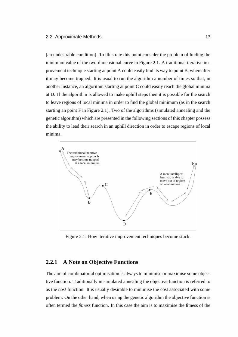
(an undesirable condition). To illustrate this point consider the problem of finding the
minimum value of the two-dimensional curve in Figure 2.1. A traditional iterative im-
provement technique starting at point A could easily find its way to point B, whereafter
it may become trapped. It is usual to run the algorithm a number of times so that, in
another instance, an algorithm starting at point C could easily reach the global minima
at D. If the algorithm is allowed to make uphill steps then it is possible for the search
to leave regions of local minima in order to find the global minimum (as in the search
starting an point F in Figure 2.1). Two of the algorithms (simulated annealing and the
genetic algorithm) which are presented in the following sections of this chapter possess
the ability to lead their search in an uphill direction in order to escape regions of local
minima.
A more intelligent
move out of regionsheuristic is able to
of local minima.
A
C
E
F
The traditional iterativeimprovement approach
may become trappedat a local minimum.
B
D
Figure 2.1: How iterative improvement techniques become stuck.
2.2.1 A Note on Objective Functions
The aim of combinatorial optimisation is always to minimise or maximise some objec-
tive function. Traditionally in simulated annealing the objective function is referred to
as thecostfunction. It is usually desirable to minimise the cost associated with some
problem. On the other hand, when using the genetic algorithm the objective function is
often termed thefitnessfunction. In this case the aim is to maximise the fitness of the
14 Chapter 2. Combinatorial Optimisation
solutions to the problem. It should be noted that a minimisation problem can always be
converted to a maximisation one simply by negating the objective function. Addition-
ally, it should be noted that it is generally trivial to convert a minimisation algorithm
into a maximisation one simply by changing the evaluation technique of the algorithm.
2.2.2 Simulated Annealing
As indicated above, simulated annealing is based on the concept of annealing. In
physics, the term annealing describes the process of slowly cooling a heated metal
in order to attain a “minimum energy state”. A heated metal is said to be in a state
of “high energy”. The molecules in a metal at a sufficiently high temperature move
freely with respect to each other, however, when the metal is cooled, the molecules
lose their thermal mobility. If the metal is cooled slowly, a “minimum energy state”
will be achieved. If, however, the metal is not cooled slowly, the metal will remain in
an intermediate energy state and will contain imperfections. For example, “quench-
ing” is the process of cooling a hot metal very rapidly. Metal that has been quenched
commonly has the property that it is brittle because of the unordered structure of its
molecules. In order to apply the analogy of annealing in physics to the field of combi-
natorial optimisation it is useful to think of the slowly cooled metal as having reached
a crystalline structure in which the molecules are ordered and the energy is low. This
is analogous to the optimal solution to a problem which is “ordered” and represents
the lowest “cost” to solve the problem being optimised (assuming, of course, that the
minimum cost is sought).
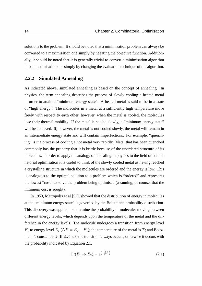
In 1953, Metropolis et al [52], showed that the distribution of energy in molecules
at the “minimum energy state” is governed by the Boltzmann probability distribution.
This discovery was applied to determine the probability of molecules moving between
different energy levels, which depends upon the temperature of the metal and the dif-
ference in the energy levels. The molecule undergoes a transition from energy level
E1 to energy levelE2 (∆E = E2 − E1); the temperature of the metal isT ; and Boltz-
mann’s constant isk. If ∆E < 0 the transition always occurs, otherwise it occurs with
the probability indicated by Equation 2.1.
Pr(E1 ⇒ E2) = e(−∆E
kT ) (2.1)
2.2. Approximate Methods 15
Probability
Energy Difference
Probability
Temperature
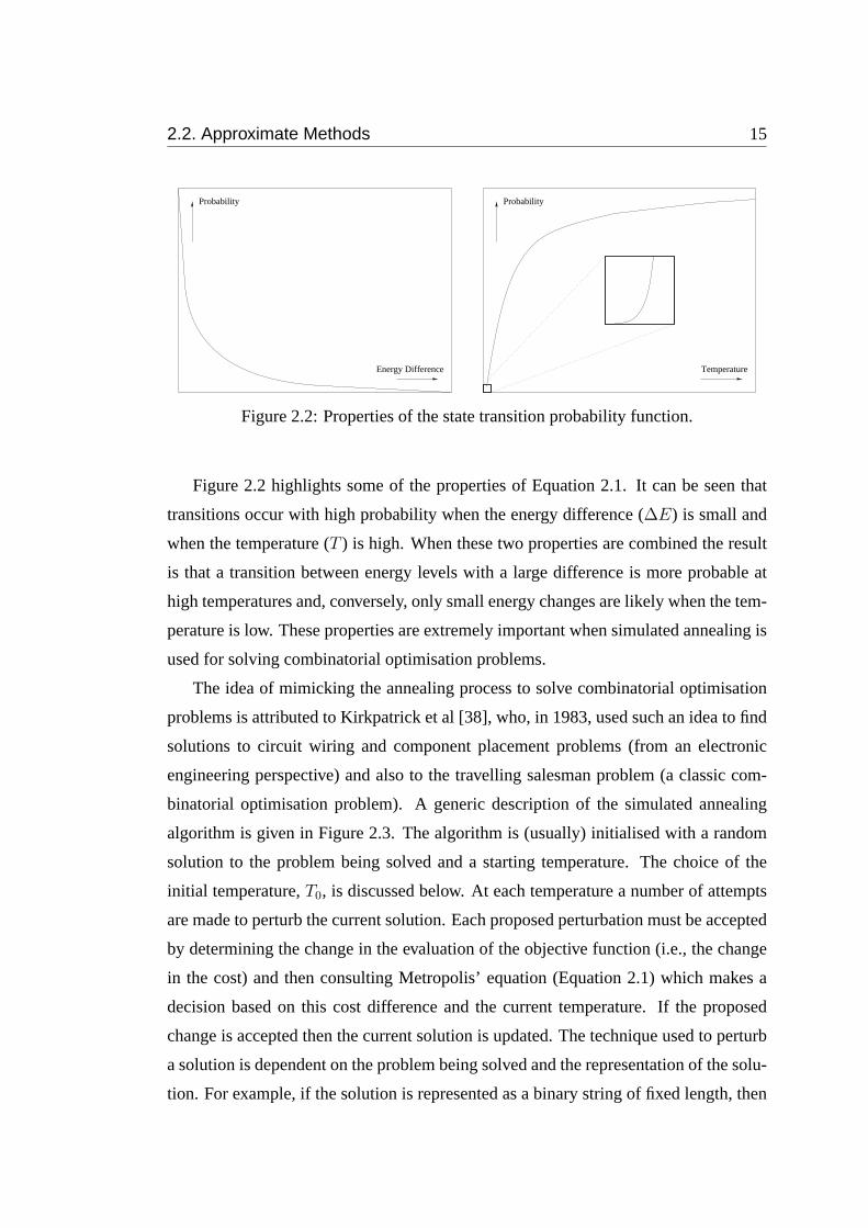
Figure 2.2: Properties of the state transition probability function.
Figure 2.2 highlights some of the properties of Equation 2.1. It can be seen that
transitions occur with high probability when the energy difference (∆E) is small and
when the temperature (T ) is high. When these two properties are combined the result
is that a transition between energy levels with a large difference is more probable at
high temperatures and, conversely, only small energy changes are likely when the tem-
perature is low. These properties are extremely important when simulated annealing is
used for solving combinatorial optimisation problems.
The idea of mimicking the annealing process to solve combinatorial optimisation
problems is attributed to Kirkpatrick et al [38], who, in 1983, used such an idea to find
solutions to circuit wiring and component placement problems (from an electronic
engineering perspective) and also to the travelling salesman problem (a classic com-
binatorial optimisation problem). A generic description of the simulated annealing
algorithm is given in Figure 2.3. The algorithm is (usually) initialised with a random
solution to the problem being solved and a starting temperature. The choice of the
initial temperature,T0, is discussed below. At each temperature a number of attempts
are made to perturb the current solution. Each proposed perturbation must be accepted
by determining the change in the evaluation of the objective function (i.e., the change
in the cost) and then consulting Metropolis’ equation (Equation 2.1) which makes a
decision based on this cost difference and the current temperature. If the proposed
change is accepted then the current solution is updated. The technique used to perturb
a solution is dependent on the problem being solved and the representation of the solu-
tion. For example, if the solution is represented as a binary string of fixed length, then
16 Chapter 2. Combinatorial Optimisation
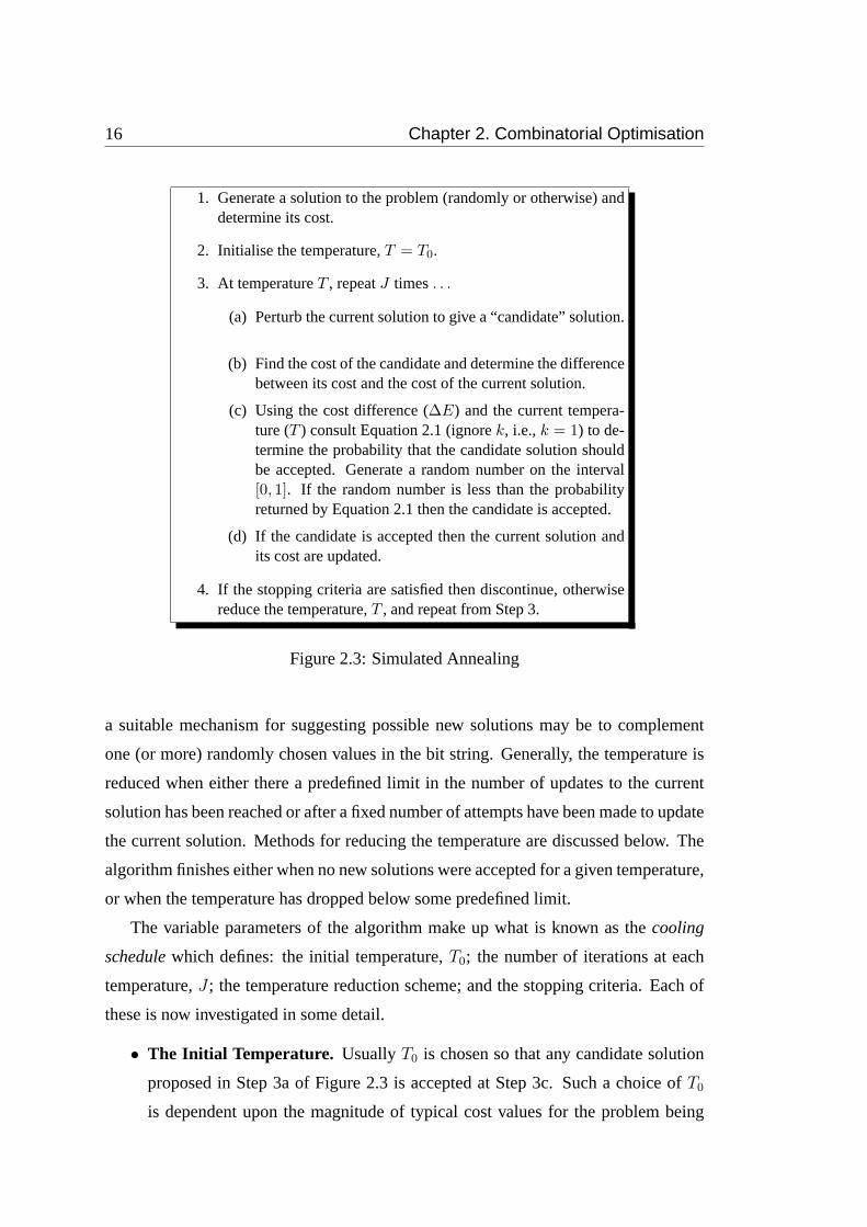
1. Generate a solution to the problem (randomly or otherwise) anddetermine its cost.
2. Initialise the temperature,T = T0.
3. At temperatureT , repeatJ times. . .
(a) Perturb the current solution to give a “candidate” solution.
(b) Find the cost of the candidate and determine the differencebetween its cost and the cost of the current solution.
(c) Using the cost difference (∆E) and the current tempera-ture (T ) consult Equation 2.1 (ignorek, i.e.,k = 1) to de-termine the probability that the candidate solution shouldbe accepted. Generate a random number on the interval[0, 1]. If the random number is less than the probabilityreturned by Equation 2.1 then the candidate is accepted.
(d) If the candidate is accepted then the current solution andits cost are updated.
4. If the stopping criteria are satisfied then discontinue, otherwisereduce the temperature,T , and repeat from Step 3.
Figure 2.3: Simulated Annealing
a suitable mechanism for suggesting possible new solutions may be to complement
one (or more) randomly chosen values in the bit string. Generally, the temperature is
reduced when either there a predefined limit in the number of updates to the current
solution has been reached or after a fixed number of attempts have been made to update
the current solution. Methods for reducing the temperature are discussed below. The
algorithm finishes either when no new solutions were accepted for a given temperature,
or when the temperature has dropped below some predefined limit.
The variable parameters of the algorithm make up what is known as thecooling
schedulewhich defines: the initial temperature,T0; the number of iterations at each
temperature,J ; the temperature reduction scheme; and the stopping criteria. Each of
these is now investigated in some detail.
• The Initial Temperature. UsuallyT0 is chosen so that any candidate solution
proposed in Step 3a of Figure 2.3 is accepted at Step 3c. Such a choice ofT0
is dependent upon the magnitude of typical cost values for the problem being
2.2. Approximate Methods 17
solved, or, more specifically, the magnitude of the largest expected cost differ-
ence between two solutions to the problem being solved. To ensure that the prob-
ability that the transition occurs is close to one,T0 must be significantly greater
than the largest expected cost difference (as shown by the following equations).
Pr(E1 ⇒ E2) → 1 ⇔ e(−∆E
T ) → 1
⇔ ∆E
T→ 0
⇔ ∆E ¿ T
The plot of Probability versus Temperature in Figure 2.2 shows the curve
being relatively flat for high temperatures. It is important not to choose an initial
temperature which is too high since this will cause the algorithm to run for longer
than necessary since most of the useful transitions are made in the temperature
ranges of the steep part of the curve.
Also, although not stated previously, it is vital that the temperature remain
greater than zero since this assumption is made when calculating the probability
from Equation 2.1. Hence,T0 must be greater than zero.
• Iterations For Each T . The number of iterations at each temperature is equiv-
alent to the number of candidate solutions considered for each temperature (re-
ferred to asJ in Figure 2.3). The value should be large but not so large that the
performance of the algorithm is hindered. One value suggested in the literature
is 100N , whereN is the number of variables in the problem being solved.
If, in Step 3a, a random alteration is made to the solution in order to generate
a new candidate, the number of candidates trialled should be greater than if a
more intelligent and problem specific perturbation function is used.
• Temperature Reduction. In theory, the rate at which temperature dissipates
from a metal is governed by complicated differential equations. For the purposes
of simulated annealing, two simple models are most commonly used. The first,
and most simplistic, is a linear cooling model. In the linear model both an initial
temperature (T0) and a final temperature (T∞) must be defined. The difference
between these two (T0 − T∞) is then divided byJ to determine how much the
18 Chapter 2. Combinatorial Optimisation
temperature is reduced by at Step 4 (Figure 2.3). The temperature at iterationk
is defined by Equations 2.2 and 2.3.
Tk = T0 − k ·(
T0 − T∞J
)(2.2)
= Tk−1 −(
T0 − T∞J
)(2.3)
The second method of temperature reduction is exponential decay. This is
a more accurate model of the true thermal dynamics in a heated metal than the
linear model. At each iteration the temperature is reduced by multiplying with a
factor,λ < 1. Equations 2.4 and 2.5 describe the temperature at iterationk.
Tk = λk · T0 (2.4)
= λ · Tk−1 (2.5)
Because of its closer approximation to the expected temperature reduction in
a practical sense, the exponential method is used in all work reported here.
• Stopping Criteria. The stopping criteria define when the algorithm should ter-
minate. Possibilities are: a minimum temperature (eg,T∞) has been reached; a
certain number of temperature reductions have occurred; or the current solution
has not changed for a number of iterations. The latter is often the best option
as any candidate solutions will not be accepted (unless they are better than the
current one) when the temperature is very low. This is because the probability
of acceptance (as defined by Equation 2.1) is negligible.
2.2.3 Genetic Algorithms
As may be evident from the simulated annealing algorithm, mathematicians often look
to other areas in search of inspiration for new techniques which can be modelled for the
purpose of optimisation. While simulated annealing is derived from the field of chem-
ical physics, the genetic algorithm is based upon another “scientific” notion, namely
Darwinian evolution theory. The genetic algorithm is modelled on a relatively simple
interpretation of the evolutionary process, however, it has proven to be a reliable and
powerful optimisation technique in a wide variety of applications.
2.2. Approximate Methods 19
It was Holland [31] in his 1975 paper, who first proposed the use of genetic al-
gorithms for problem solving. Goldberg [25] and DeJong [14] were also pioneers in
the area of applying genetic processes to optimisation. Over the past twenty years
numerous applications and adaptations have appeared in the literature. Three papers
containing applications to the field of cryptanalysis are worthy of mention here. The
first, by Matthews [47] and the second, by Spillman et al [71], are used in attacks on the
transposition cipher and the substitution cipher, respectively (see Chapter 3 for more
details). The third paper, by Spillman [71], attempts an attack on the knapsack cipher
(this work is covered in detail in Chapter 5).
Consider a pool of genes which have the ability to reproduce, are able to adapt to
environmental changes and, depending on their individual strengths, have varying life-
spans. In such an environment only the fittest will survive and reproduce giving, over
time, genes that are stronger and more resilient to conditional changes. After a certain
amount of time the surviving genes could be considered “optimal” in some sense. This
is the model used by the genetic algorithm, where the gene is the representation of a
solution to the problem being optimised. Traditionally, genetic algorithms have solu-
tions represented by binary strings. However, not all problems have solutions which
are easily represented in binary (especially if the structure of the binary string is to be
“meaningful”). To avoid this limiting property a more general area known asevolu-
tionary programminghas been developed. An evolutionary program may make use of
arbitrary data structures in order to represent the solution. For simplicity all algorithms
described in this thesis which use the evolutionary heuristics presented in this section
are referred to as “genetic algorithms”, although, from a purist’s perspective, this may
not be strictly accurate.
As with any optimisation technique there must be a method of assessing each so-
lution. In keeping with the evolutionary theme, the assessment technique used by a
genetic algorithm is usually referred to as the “fitness function”. As was pointed out
above, the aim is always to maximise the fitness of the solutions in the solution pool.
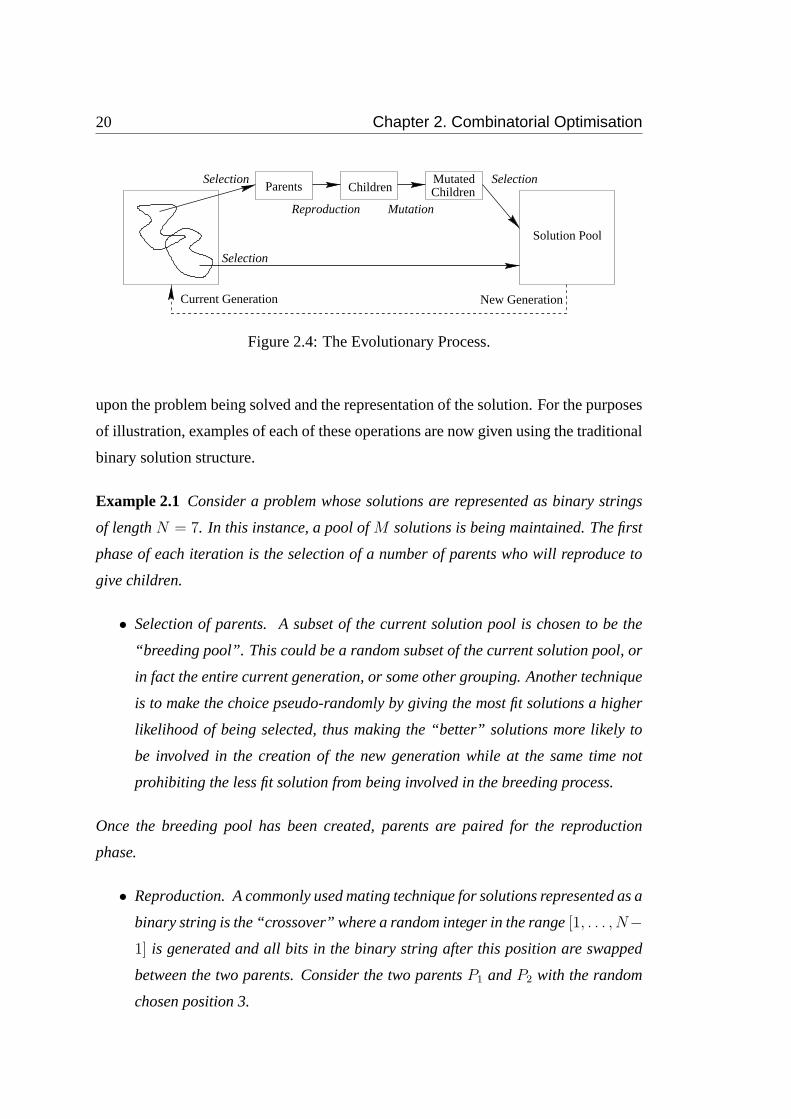
Figure 2.4 gives an indication of the evolutionary processes used by the genetic
algorithm. During each iteration of the algorithm the processes of selection, reproduc-
tion and mutation each take place in order to produce the next generation of solutions.
The actual method used to perform each of these operations is very much dependent
20 Chapter 2. Combinatorial Optimisation
MutationReproduction
New GenerationCurrent Generation
Parents ChildrenSelectionSelection
Selection
Solution Pool
MutatedChildren
Figure 2.4: The Evolutionary Process.
upon the problem being solved and the representation of the solution. For the purposes
of illustration, examples of each of these operations are now given using the traditional
binary solution structure.
Example 2.1 Consider a problem whose solutions are represented as binary strings
of lengthN = 7. In this instance, a pool ofM solutions is being maintained. The first
phase of each iteration is the selection of a number of parents who will reproduce to
give children.
• Selection of parents.A subset of the current solution pool is chosen to be the
“breeding pool”. This could be a random subset of the current solution pool, or
in fact the entire current generation, or some other grouping. Another technique
is to make the choice pseudo-randomly by giving the most fit solutions a higher
likelihood of being selected, thus making the “better” solutions more likely to
be involved in the creation of the new generation while at the same time not
prohibiting the less fit solution from being involved in the breeding process.
Once the breeding pool has been created, parents are paired for the reproduction
phase.
• Reproduction.A commonly used mating technique for solutions represented as a
binary string is the “crossover” where a random integer in the range[1, . . . , N−1] is generated and all bits in the binary string after this position are swapped
between the two parents. Consider the two parentsP1 andP2 with the random
chosen position 3.
2.2. Approximate Methods 21
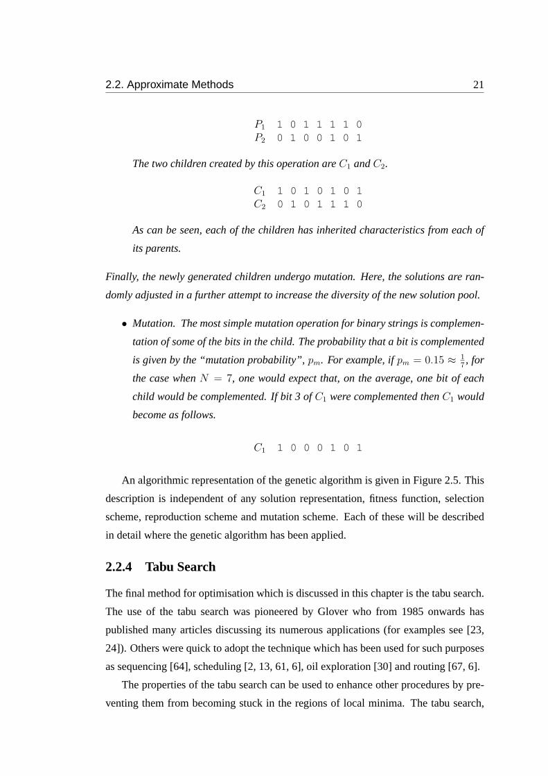
P1 1 0 1 1 1 1 0P2 0 1 0 0 1 0 1
The two children created by this operation areC1 andC2.
C1 1 0 1 0 1 0 1C2 0 1 0 1 1 1 0
As can be seen, each of the children has inherited characteristics from each of
its parents.
Finally, the newly generated children undergo mutation. Here, the solutions are ran-
domly adjusted in a further attempt to increase the diversity of the new solution pool.
• Mutation. The most simple mutation operation for binary strings is complemen-
tation of some of the bits in the child. The probability that a bit is complemented
is given by the “mutation probability”,pm. For example, ifpm = 0.15 ≈ 17, for
the case whenN = 7, one would expect that, on the average, one bit of each
child would be complemented. If bit 3 ofC1 were complemented thenC1 would
become as follows.
C1 1 0 0 0 1 0 1
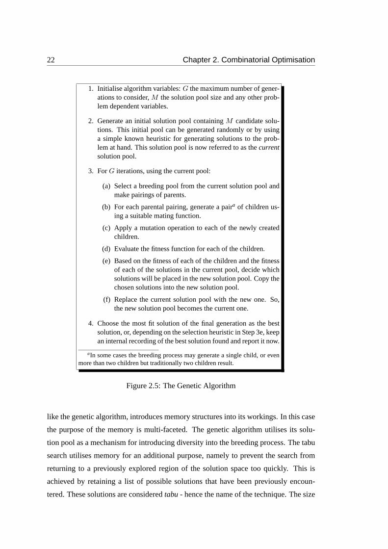
An algorithmic representation of the genetic algorithm is given in Figure 2.5. This
description is independent of any solution representation, fitness function, selection
scheme, reproduction scheme and mutation scheme. Each of these will be described
in detail where the genetic algorithm has been applied.
2.2.4 Tabu Search
The final method for optimisation which is discussed in this chapter is the tabu search.
The use of the tabu search was pioneered by Glover who from 1985 onwards has
published many articles discussing its numerous applications (for examples see [23,
24]). Others were quick to adopt the technique which has been used for such purposes
as sequencing [64], scheduling [2, 13, 61, 6], oil exploration [30] and routing [67, 6].
The properties of the tabu search can be used to enhance other procedures by pre-
venting them from becoming stuck in the regions of local minima. The tabu search,
22 Chapter 2. Combinatorial Optimisation
1. Initialise algorithm variables:G the maximum number of gener-ations to consider,M the solution pool size and any other prob-lem dependent variables.
2. Generate an initial solution pool containingM candidate solu-tions. This initial pool can be generated randomly or by usinga simple known heuristic for generating solutions to the prob-lem at hand. This solution pool is now referred to as thecurrentsolution pool.
3. ForG iterations, using the current pool:
(a) Select a breeding pool from the current solution pool andmake pairings of parents.
(b) For each parental pairing, generate a paira of children us-ing a suitable mating function.
(c) Apply a mutation operation to each of the newly createdchildren.
(d) Evaluate the fitness function for each of the children.
(e) Based on the fitness of each of the children and the fitnessof each of the solutions in the current pool, decide whichsolutions will be placed in the new solution pool. Copy thechosen solutions into the new solution pool.
(f) Replace the current solution pool with the new one. So,the new solution pool becomes the current one.
4. Choose the most fit solution of the final generation as the bestsolution, or, depending on the selection heuristic in Step 3e, keepan internal recording of the best solution found and report it now.
aIn some cases the breeding process may generate a single child, or evenmore than two children but traditionally two children result.
Figure 2.5: The Genetic Algorithm
like the genetic algorithm, introduces memory structures into its workings. In this case
the purpose of the memory is multi-faceted. The genetic algorithm utilises its solu-
tion pool as a mechanism for introducing diversity into the breeding process. The tabu
search utilises memory for an additional purpose, namely to prevent the search from
returning to a previously explored region of the solution space too quickly. This is
achieved by retaining a list of possible solutions that have been previously encoun-
tered. These solutions are consideredtabu- hence the name of the technique. The size
2.3. Summary 23
of the tabu list is one of the parameters of the tabu search.
The tabu search also contains mechanisms for controlling the search. The tabu list
ensures that some solutions will be unacceptable, however, the restriction provided by
the tabu list may become too limiting in some cases causing the algorithm to become
trapped at a locally optimum solution. The tabu search introduces the notion ofaspi-
ration criteria in order to overcome this problem. The aspiration criteria over-ride the
tabu restrictions making it possible to broaden the search for the global optimum.
Much of the implementation of the tabu search is problem specific - i.e., the mech-
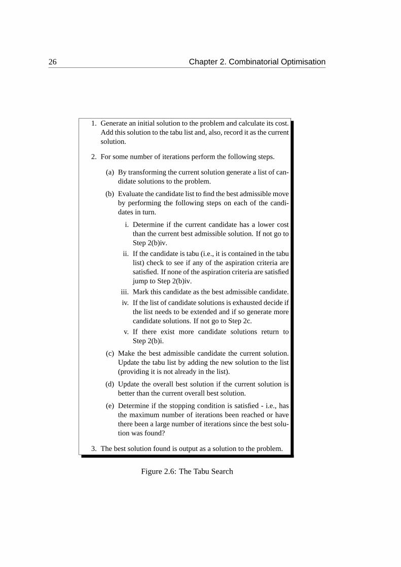
anisms used depend heavily upon the type of problem being solved. Figure 2.6 gives
a general description of the tabu search. An initial solution is generated (usually ran-
domly). The tabu list is initialised with the initial solution. A number of iterations are
performed which attempt to update the current solution with a better one, subject to
the restrictions of the tabu list. In each iteration a list of candidate solutions is pro-
posed. These solutions are obtained in a similar fashion to the perturbation technique
used in simulated annealing and the mutation operation used in the genetic algorithm.
The most admissible solution is selected from the candidate list using the five steps
in item 2b in Figure 2.6. The current solution is updated with the most admissible
one and the new current solution is added to the tabu list. The algorithm stops after
a fixed number of iterations or when a better solution has been found for a number of
iterations.
2.3 Summary
This chapter has introduced the reader to several of the essential concepts involved in
the field of combinatorial optimisation. Evidence justifying the need for combinatorial
optimisation algorithms has been presented and a number of algorithms detailed.
The theory of NP-completeness has been introduced. This theory describes a bound
on the difficulty of solving a class of problems, namely the NP-complete decision
problems. This theory is necessary in order to understand the need for optimisation
heuristics which, although seeming ad-hoc in some ways, are the only known methods
for finding suitable solutions to problems which are NP-hard.
The difference between exact and approximate optimisation algorithms is discussed,

24 Chapter 2. Combinatorial Optimisation
along with the reasoning behind the suitability of each of these techniques for particu-
lar applications. Exact algorithms are usually computationally intensive and, therefore,
infeasible for many applications. Approximate algorithms, on the other hand, apply
search heuristics designed to scan the solution space in a meaningful manner, avoiding
regions of local minima, to find a suitable solution. Three such algorithms have been
described in detail: simulated annealing, the genetic algorithm and the tabu search.
The amount of detail given should be sufficient to enable the implementation of any
of these techniques in any suitable application. Each of the three techniques possesses
unique properties which make it useful in a broad spectrum of applications. References
to published material relating to the theory and applications of these techniques have
also been documented.
Simulated annealing mimics the process of annealing in metals using the analogy
of a solution to the structure of the molecules in the heated metal. When the tem-
perature is high the molecules move at random and appear to have little order. This
may represent an initial random guess at a solution to an optimisation problem. After
some time, as the temperature slowly cools, the molecules move toward a more ordered
structure, the aim of annealing being to produce a crystalline structure in the molecules.
The analogy to optimisation is still present so that as the algorithm progresses a more
ordered solution (hopefully one similar to the optimum) is obtained.
The genetic algorithm is an attempt to use Darwin’s evolutionary model in the field
of optimisation which has proven to be remarkably successful. A pool of solutions
breed, and mutate in a survival of the fittest regime. Solutions not considered suitable
(classified by the optimisation problem’s objective function) die off so that, over time,
the solution pool contains good solutions to the problem. Initially intended to oper-
ate on problems whose solutions could be represented as a binary string, the genetic
algorithm has grown to cover the field known as “evolutionary programming” where
an arbitrary solution representation can be utilised, provided suitable genetic operators
can be created.
The tabu search incorporates techniques for ensuring that the solutions considered
in the search are diverse. This is achieved by maintaining a tabu list which contains
a list of solutions which have been visited by the search previously and may not be
accepted again, at least not until a certain amount of time has passed. However, by
2.3. Summary 25
specifying aspiration criteria, the tabu list can be overridden in order to ensure that
solutions which are believed to be good may be accepted.
The techniques presented in this chapter will be utilised throughout the remainder
of this thesis, in both cryptanalytic and cryptographic applications. In Chapter 3 the
classical substitution and transposition-type ciphers are cryptanalysed. In Chapter 4
it is shown that these techniques can be incorporated with other, more specialised al-
gorithms, in order to obtain some improvement. Chapter 5 presents an example of an
application where these techniques are of little use. This further belies the necessity
for understanding which applications are suited to combinatorial optimisation. This
is especially true in the field of cryptology since ciphers are designed to be infeasible
to solve. A method of systematically generating highly nonlinear Boolean functions
using a genetic algorithm is presented in Chapter 6.
26 Chapter 2. Combinatorial Optimisation
1. Generate an initial solution to the problem and calculate its cost.Add this solution to the tabu list and, also, record it as the currentsolution.
2. For some number of iterations perform the following steps.
(a) By transforming the current solution generate a list of can-didate solutions to the problem.
(b) Evaluate the candidate list to find the best admissible moveby performing the following steps on each of the candi-dates in turn.
i. Determine if the current candidate has a lower costthan the current best admissible solution. If not go toStep 2(b)iv.
ii. If the candidate is tabu (i.e., it is contained in the tabulist) check to see if any of the aspiration criteria aresatisfied. If none of the aspiration criteria are satisfiedjump to Step 2(b)iv.
iii. Mark this candidate as the best admissible candidate.
iv. If the list of candidate solutions is exhausted decide ifthe list needs to be extended and if so generate morecandidate solutions. If not go to Step 2c.
v. If there exist more candidate solutions return toStep 2(b)i.
(c) Make the best admissible candidate the current solution.Update the tabu list by adding the new solution to the list(providing it is not already in the list).
(d) Update the overall best solution if the current solution isbetter than the current overall best solution.
(e) Determine if the stopping condition is satisfied - i.e., hasthe maximum number of iterations been reached or havethere been a large number of iterations since the best solu-tion was found?
3. The best solution found is output as a solution to the problem.
Figure 2.6: The Tabu Search
Chapter 3
Classical Ciphers
Classical ciphers were first used hundreds of years ago. So far as security is concerned,
they are no match for today’s ciphers, however, this does not mean that they are any less
important to the field of cryptology. Their importance stems from the fact that most of
the ciphers in common use today utilise the operations of the classical ciphers as their
building blocks. For example, the Data Encryption Standard (DES), an encryption
algorithm used widely in the finance community throughout the world, uses only three
very simple operators, namely substitution, permutation (transposition) and bit-wise
exclusive-or (admittedly, in a rather complicated fashion). Given their simplicity, and
the fact that they are used to construct other ciphers, the classical ciphers are usually
the first ones considered when researching new attack techniques such as the ones
discussed in this chapter.
Many flavours of classical ciphers exist, although most fall into one of two broad
categories: substitution ciphers and transposition (permutation) ciphers. In this chap-
ter three specific examples of ciphers are considered. Two of the ciphers considered
fall into the category of substitution ciphers: the simple (or monoalphabetic) substi-
tution cipher and the polyalphabetic substitution cipher; and the other is an example
of a transposition cipher. Detailed descriptions of each of these ciphers are given in
Appendix A. The appendix also provides worked examples of each of the different
ciphers.
Previously, Forsyth and Safavi-Naini (in [18]) have published an attack on the sim-
ple substitution cipher using simulated annealing and Spillman et al (in [73]) presented
an attack (again, on the simple substitution cipher) using a genetic algorithm. Also, an
attack on the transposition cipher was proposed by Matthews (in [47]) using a genetic
27
28 Chapter 3. Classical Ciphers
algorithm. These attacks have been re-implemented in this chapter in order to obtain
a comparison of the techniques and also to evaluate a third technique, namely the tabu
search. Attacks on both the simple substitution cipher and the transposition cipher were
implemented using all three optimisation heuristics described in Chapter 2: i.e., simu-
lated annealing, the genetic algorithm and the tabu search. This involved the design of
an attack on the substitution cipher using the tabu search and the design of attacks on
the transposition cipher using simulated annealing and the tabu search. The previously
published attacks were enhanced and modified in order that an accurate comparison of
the three techniques could be obtained. Attacks on the simple substitution cipher are
described in detail in Section 3.1 and attacks on the transposition cipher are described
in Section 3.3.
Each of the three techniques was compared based on three criteria: the amount
of known ciphertext available to the attack; the number of keys considered before the
correct solution was found; and the time required by the attack to determine the correct
solution. The results are presented graphically in order to achieve a clear comparison.
The results for the simple substitution cipher are given in Section 3.1.5 and the results
for the transposition cipher are given in Section 3.3.5.
In addition to the comparison of the three optimisation heuristics for attacks on the
simple substitution cipher and the transposition cipher, a new attack is presented on
the polyalphabetic substitution cipher. Because of the structure of the cipher, it is well
suited to an attack based on a parallel heuristic. In Section 3.2 a parallel technique
for attacking the polyalphabetic substitution cipher is presented which makes use of
a parallel genetic algorithm. Although parallel genetic algorithms have been applied
widely in other areas, especially numerical optimisation (see [8, 20] for examples), this
is the first application to the field of cryptanalysis (to the best of the author’s knowl-
edge). This technique is shown to be highly effective and the results are presented in
Section 3.2.2.
Techniques for determining the period of a polyalphabetic substitution cipher are
described in Appendix A. In Section 3.2 an additional technique is described which
makes use of the parallel heuristic described in the same section. Results highlighting
the effectiveness of this approach are also given.
Note that all experiments presented in this chapter were performed on text using
3.1. Attacks on the Simple Substitution Cipher 29
a 27 character alphabet, i.e., A – Z, and the space character. All punctuation and
structure (sentences/paragraphs) has been removed from the text before encryption.
Any two words are separated by a single space character.
3.1 Attacks on the Simple Substitution Cipher
The general strategy with the two substitution ciphers is to substitute symbols from the
plaintext alphabet with different symbols from the ciphertext alphabet(s). The weak-
ness with this strategy is that character frequency distributions are not significantly
altered by the encryption process. Thus, most attacks on substitution ciphers attempt
to match the character frequency statistics of the encrypted message with those of some
known language (for example, English). Character frequency statistics (orn-grams)
indicate the frequency distribution of all possible instances ofn adjacent characters
(for example,THE is a very common 3-gram (ortrigram) in the English language).
Examples A.1 and A.2 (from Appendix A) illustrate how then-gram statistics are
maintained during encryption.
The attack on the simple substitution cipher is particularly simple since the fre-
quency of anyn-gram in the plaintext (or unencrypted) message will correspondex-
actly to the frequency of the corresponding encrypted version in the ciphertext. The
search for the correspondingn-gram frequencies can be automated using combinato-
rial optimisation algorithms such as those described in Chapter 2. Here, a number of
methods are utilised in attacks in the simple substitution cipher. As previously indi-
cated, a method of assessing intermediate solutions (in the search for the optimum) is
required.
A major factor influencing the success of an attack on the simple substitution cipher
(or any cipher where the attack is based onn-gram statistics of the language) is the
length of the intercepted ciphertext message which is being cryptanalysed. The amount
of ciphertext required in order to recover the entire key (with a high degree of certainty)
varies depending on the type of cipher. From Figure 3.1 it can be seen that for a
message of 1000 characters it is possible to recover 26 out of the 27 key elements
on the average. Note that in practice it is impossible to find a simple substitution
cipher key which differs in exactly one place from the correct key. However it is not
30 Chapter 3. Classical Ciphers
necessary to recover every element of the key in order to obtain a message that is
readable. Table 3.1 shows the relative frequency of each of the characters in a sample
of English taken from the book “20000 Leagues Under the Sea” by Jules Verne. A fact
evident in almost all attacks on substitution ciphers is that the most frequent characters
are decrypted first. Table 3.1 also shows the amount of message that will have been
recovered after each of the characters is discovered (making the unrealistic assumption
that the characters are discovered in order from most frequent to least frequent). It can
be seen that approximately fifty percent of the message can be recovered by correctly
determining the key element for the five most frequent characters in the intercepted
message. Also, the eleven most infrequent characters account for only ten percent of
the message (on the average).
3.1.1 Suitability Assessment
Naturally, the technique used to compare candidate keys to the simple substitution
cipher is to comparen-gram statistics of the decrypted message with those of the lan-
guage (which are assumed known). Equation 3.1 is a general formula used to determine
the suitability of a proposed key (k) to a simple substitution cipher. Here,A denotes
the language alphabet (i.e., for English,{A, . . ., Z, _}, where_ represents the space
symbol),K andD denote known language statistics and decrypted message statistics,
respectively, and the indicesu, b andt denote the unigram, bigram and trigram statis-
tics, respectively. The values ofα, β andγ allow assigning of different weights to each
of the threen-gram types.
Ck = α · ∑
i∈A
∣∣∣Ku(i) −Du
(i)
∣∣∣
+ β · ∑
i,j∈A
∣∣∣Kb(i,j) −Db
(i,j)
∣∣∣ (3.1)
+ γ · ∑
i,j,k∈A
∣∣∣Kt(i,j,k) −Dt
(i,j,k)
∣∣∣
Forsyth and Safavi-Naini, in their simulated annealing attack on the substitution
cipher [18] and Jakobsen in his attack [33] use a very similar evaluation, namely the
one in Equation 3.2. This formula is based purely upon bigram statistics which is often

3.1. Attacks on the Simple Substitution Cipher 31
Frequency (%)Order Letter Relative Cumulative
1 _ 18.4820 18.48202 E 10.3320 28.81403 T 7.8395 36.65354 A 6.6284 43.28195 O 6.0091 49.29096 I 5.7941 55.08507 N 5.7526 60.83768 S 5.3997 66.23739 H 4.8210 71.0583
10 R 4.5744 75.632711 D 3.4530 79.085712 L 3.2366 82.322313 U 2.4719 84.794114 C 2.2742 87.068315 M 1.9853 89.053716 F 1.9242 90.977817 W 1.9183 92.896118 P 1.5438 94.439919 G 1.4424 95.882320 Y 1.2656 97.147921 B 1.2026 98.350522 V 0.7474 99.097923 K 0.5482 99.646124 X 0.1466 99.792825 Q 0.0851 99.877926 J 0.0667 99.944527 Z 0.0555 100.0000
Table 3.1: English language characteristics.
sufficient for attacks on the simple substitution cipher.
Ck =∑
i,j∈A
∣∣∣Kb(i,j) −Db
(i,j)
∣∣∣ (3.2)
Spillman et al [73], use a different formula again (see Equation 3.3). This equation
is based on unigram and bigram statistics.
Ck ∝ ∑
i∈A
∣∣∣Ku(i) −Du
(i)
∣∣∣ +∑
i,j∈A
∣∣∣Kb(i,j) −Db
(i,j)
∣∣∣ (3.3)
The only difference between these assessment functions is the inclusion of differ-
ent statistics (Equation 3.2 is equal to Equation 3.1 whenα = γ = 0). In general, the
32 Chapter 3. Classical Ciphers
larger then-grams, the more accurate the assessment is likely to be. It is usually an
expensive task to calculate the trigram statistics - this is, perhaps, why they are omitted
in Equations 3.2 and 3.3. The complexity of determining the fitness isO(N3) (where
N is the alphabet size) when trigram statistics are being determined, compared with
O(N2) when bigrams are the largest statistics being used. Following the attack de-
scription given below there are details describing a method which can be used under
some circumstances for reducing the complexity of the cost calculation by a factor of
N . Thus a cost based on trigram statistics can be calculated with complexity propor-
tional toO(N2).
Figure 3.1 indicates the effectiveness of using differentn-grams in the evaluation
of a simple substitution cipher key. The three curves in the plot represent the per-
centage of key recovered by an attack on a simple substitution cipher using simulated
annealing (see below) versus the amount of known ciphertext used in the attack. Each
curve resulted from using the cost function in Equation 3.1 with different values of the
weightsα, β andγ. For example, the “Unigrams only” curve was obtained withα = 1
andβ = γ = 0. Each data point on each curve was determined by running the attack
on 200 different messages and three times for each message. Of the three runs for each
message only the best result was used. The value on the curve represents the average
number of key elements correctly placed (over the 200 messages). For the alphabet
being used the maximum value attainable is 27.
For small amounts of known ciphertext it is interesting to note that an attack using
a cost function based on bigrams alone is more effective than one which utilises only
trigrams (see Figure 3.1). The crossover point of the “Bigrams only” and “Trigrams
Only” curves in Figure 3.1 represents an approximate threshold value where a cost
function based purely upon trigram frequencies out-performs one based only on bigram
frequencies. The reason for the phenomenon can, in part, be gleaned by observing
the cost function in Equation 3.1. When the length of the intercepted messages is
short there are far fewer distinct bigrams or trigrams represented in the ciphertext than
the total number of possible bigrams or trigrams. WhenN = 27 there areN3 =
19683 possible trigrams (theoretically - of course not all trigrams are represented in
the English language). The maximum number of distinct trigrams in a message of
length say, 100, is 98. Thus the proportion of trigrams represented in the message
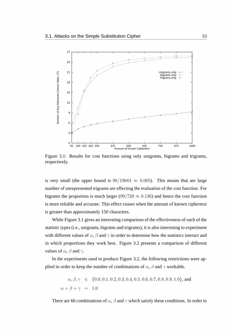
3.1. Attacks on the Simple Substitution Cipher 33
0
3
6
9
12
15
18
21
24
27
50 100 150 200 250 375 500 625 750 875 1000
Num
ber
of K
ey E
lem
ents
Cor
rect
(M
ax: 2
7)
Amount of Known Ciphertext
Unigrams onlyBigrams onlyTrigrams only
Figure 3.1: Results for cost functions using only unigrams, bigrams and trigrams,respectively.
is very small (the upper bound is98/19683 ≈ 0.005). This means that are large
number of unrepresented trigrams are effecting the evaluation of the cost function. For
bigrams the proportion is much larger (99/729 ≈ 0.136) and hence the cost function
is more reliable and accurate. This effect ceases when the amount of known ciphertext
is greater than approximately 150 characters.
While Figure 3.1 gives an interesting comparison of the effectiveness of each of the
statistic types (i.e., unigrams, bigrams and trigrams), it is also interesting to experiment
with different values ofα, β andγ in order to determine how the statistics interact and
in which proportions they work best. Figure 3.2 presents a comparison of different
values ofα, β andγ.
In the experiments used to produce Figure 3.2, the following restrictions were ap-
plied in order to keep the number of combinations ofα, β andγ workable.
α, β, γ ∈ {0.0, 0.1, 0.2, 0.3, 0.4, 0.5, 0.6, 0.7, 0.8, 0.9, 1.0}, and
α + β + γ = 1.0
There are 66 combinations ofα, β andγ which satisfy these conditions. In order to
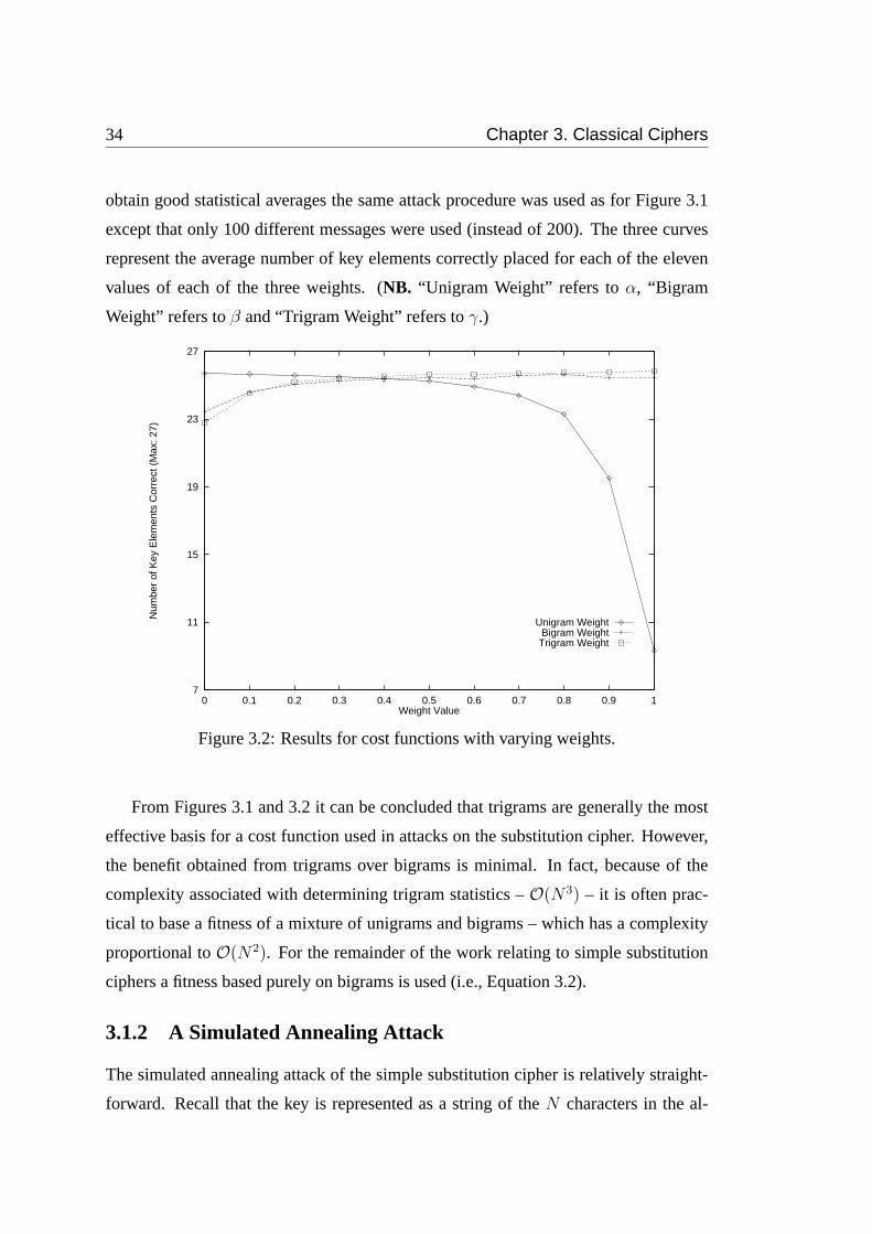
34 Chapter 3. Classical Ciphers
obtain good statistical averages the same attack procedure was used as for Figure 3.1
except that only 100 different messages were used (instead of 200). The three curves
represent the average number of key elements correctly placed for each of the eleven
values of each of the three weights. (NB. “Unigram Weight” refers toα, “Bigram
Weight” refers toβ and “Trigram Weight” refers toγ.)
7
11
15
19
23
27
0 0.1 0.2 0.3 0.4 0.5 0.6 0.7 0.8 0.9 1
Num
ber
of K
ey E
lem
ents
Cor
rect
(M
ax: 2
7)
Weight Value
Unigram WeightBigram WeightTrigram Weight
Figure 3.2: Results for cost functions with varying weights.
From Figures 3.1 and 3.2 it can be concluded that trigrams are generally the most
effective basis for a cost function used in attacks on the substitution cipher. However,
the benefit obtained from trigrams over bigrams is minimal. In fact, because of the
complexity associated with determining trigram statistics –O(N3) – it is often prac-
tical to base a fitness of a mixture of unigrams and bigrams – which has a complexity
proportional toO(N2). For the remainder of the work relating to simple substitution
ciphers a fitness based purely on bigrams is used (i.e., Equation 3.2).
3.1.2 A Simulated Annealing Attack
The simulated annealing attack of the simple substitution cipher is relatively straight-
forward. Recall that the key is represented as a string of theN characters in the al-
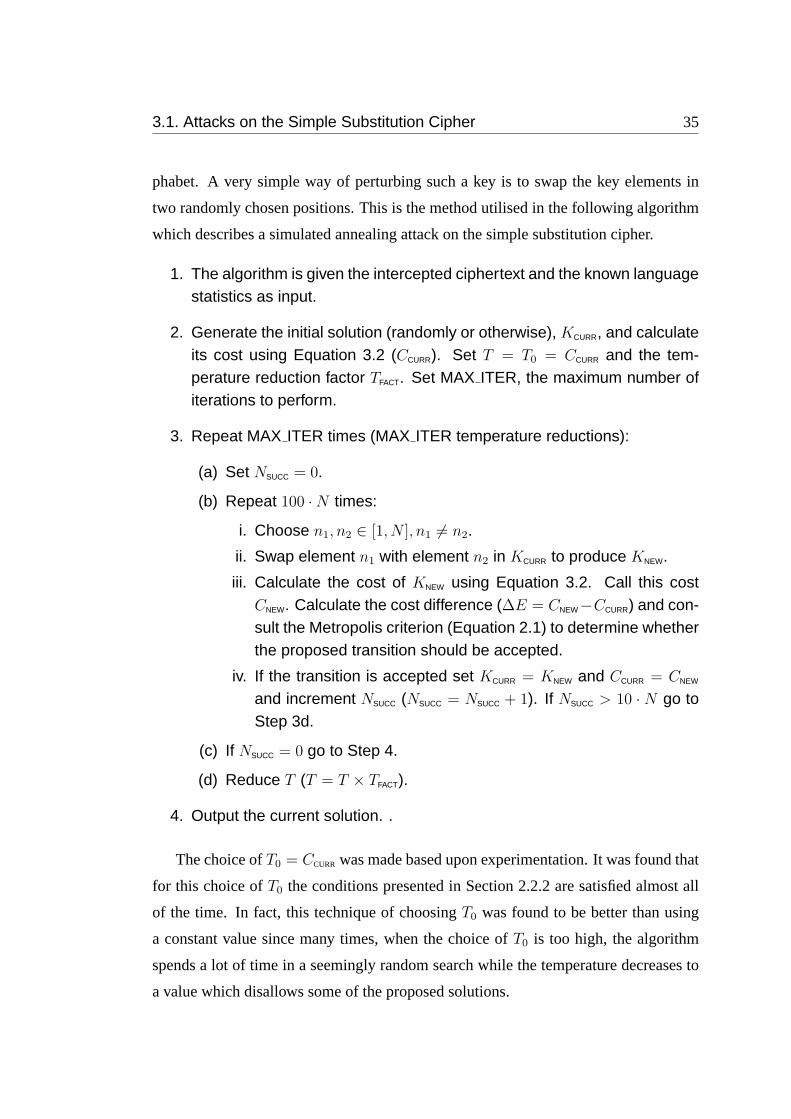
3.1. Attacks on the Simple Substitution Cipher 35
phabet. A very simple way of perturbing such a key is to swap the key elements in
two randomly chosen positions. This is the method utilised in the following algorithm
which describes a simulated annealing attack on the simple substitution cipher.
1. The algorithm is given the intercepted ciphertext and the known languagestatistics as input.
2. Generate the initial solution (randomly or otherwise), KCURR, and calculateits cost using Equation 3.2 (CCURR). Set T = T0 = CCURR and the tem-perature reduction factor TFACT. Set MAX ITER, the maximum number ofiterations to perform.
3. Repeat MAX ITER times (MAX ITER temperature reductions):
(a) Set NSUCC = 0.
(b) Repeat 100 ·N times:
i. Choose n1, n2 ∈ [1, N ], n1 6= n2.
ii. Swap element n1 with element n2 in KCURR to produce KNEW.
iii. Calculate the cost of KNEW using Equation 3.2. Call this costCNEW. Calculate the cost difference (∆E = CNEW−CCURR) and con-sult the Metropolis criterion (Equation 2.1) to determine whetherthe proposed transition should be accepted.
iv. If the transition is accepted set KCURR = KNEW and CCURR = CNEW
and increment NSUCC (NSUCC = NSUCC + 1). If NSUCC > 10 · N go toStep 3d.
(c) If NSUCC = 0 go to Step 4.
(d) Reduce T (T = T × TFACT).
4. Output the current solution. .
The choice ofT0 = CCURR was made based upon experimentation. It was found that
for this choice ofT0 the conditions presented in Section 2.2.2 are satisfied almost all
of the time. In fact, this technique of choosingT0 was found to be better than using
a constant value since many times, when the choice ofT0 is too high, the algorithm
spends a lot of time in a seemingly random search while the temperature decreases to
a value which disallows some of the proposed solutions.
36 Chapter 3. Classical Ciphers
The values100 · N (Step 3b) and10 · N (Step 3(b)iv) are parameters of the algo-
rithm which are arbitrary. They should, of course, be chosen so that a large number
of possible solutions are assessed at each temperature, but not so large that time is
wasted. By setting a limit to the number of successful updates to the solution at each
temperature, the algorithm avoids assessing too many solutions when the temperature
is high (since almost all suggested transitions are accepted at high temperatures).
As indicated above, there are circumstances under which it is possible to reduce
the complexity of the cost calculation. One such case is when comparing the cost
associated with two keys when the keys only differ in two elements (i.e., one key can
be obtained from the other key simply by swapping two elements). This is exactly
what happens in the simulated annealing algorithm above - two elements in the current
key are swapped and the new cost calculated. The difference between the cost of the
current solution and the new one (with the swapped elements) is used to determine if
the new key will be accepted.
It should be clear that when two key elements are swapped only the statistics (of the
decrypted message) for trigrams which contain one (or both) of the swapped elements
will change. Similarly, only the statistics for bigrams which contain one (or both)
of the swapped elements will change. Also, only two of the unigram statistics will
change.
Making use of this property can lead to a significant increase in the efficiency of
the simulated annealing attack. The improvement obtained using such a strategy is of
the order ofN . Table 3.2 displays the actual improvement in terms of the number of
comparisons of statistics required in the evaluation of the cost difference. The numbers
in brackets indicate the number of calculations required whenN = 27. It can be
seen that whenN = 27 the complexity of determining a cost based on trigrams is
not significantly reduced using this technique. However, for larger values ofN - for
example consider the ASCII alphabet of 256 characters - the saving is great.
This technique can be used for determining the cost difference between two keys
in any system where one key is obtained from another by swapping two elements of
the original key.
The results of the attack described in this section are compared with the attacks
using the genetic algorithm and tabu search (described below), in Section 3.1.5.
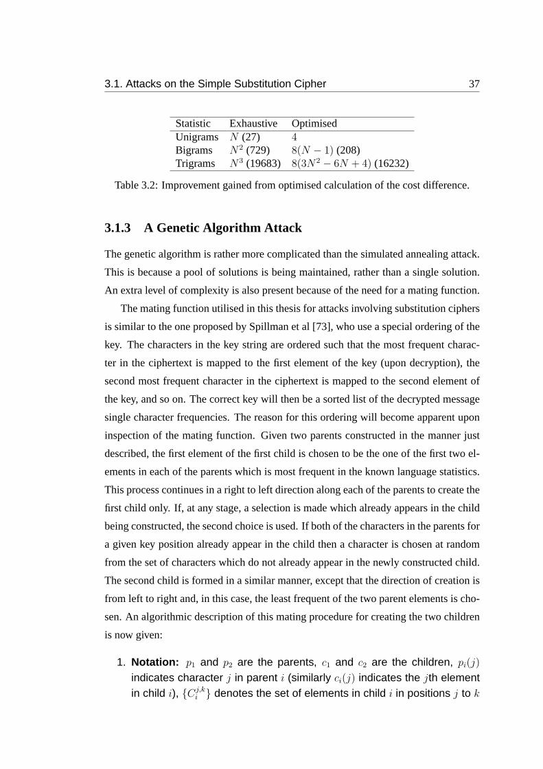
3.1. Attacks on the Simple Substitution Cipher 37
Statistic Exhaustive OptimisedUnigrams N (27) 4Bigrams N2 (729) 8(N − 1) (208)Trigrams N3 (19683) 8(3N2 − 6N + 4) (16232)
Table 3.2: Improvement gained from optimised calculation of the cost difference.
3.1.3 A Genetic Algorithm Attack
The genetic algorithm is rather more complicated than the simulated annealing attack.
This is because a pool of solutions is being maintained, rather than a single solution.
An extra level of complexity is also present because of the need for a mating function.
The mating function utilised in this thesis for attacks involving substitution ciphers
is similar to the one proposed by Spillman et al [73], who use a special ordering of the
key. The characters in the key string are ordered such that the most frequent charac-
ter in the ciphertext is mapped to the first element of the key (upon decryption), the
second most frequent character in the ciphertext is mapped to the second element of
the key, and so on. The correct key will then be a sorted list of the decrypted message
single character frequencies. The reason for this ordering will become apparent upon
inspection of the mating function. Given two parents constructed in the manner just
described, the first element of the first child is chosen to be the one of the first two el-
ements in each of the parents which is most frequent in the known language statistics.
This process continues in a right to left direction along each of the parents to create the
first child only. If, at any stage, a selection is made which already appears in the child
being constructed, the second choice is used. If both of the characters in the parents for
a given key position already appear in the child then a character is chosen at random
from the set of characters which do not already appear in the newly constructed child.
The second child is formed in a similar manner, except that the direction of creation is
from left to right and, in this case, the least frequent of the two parent elements is cho-
sen. An algorithmic description of this mating procedure for creating the two children
is now given:
1. Notation: p1 and p2 are the parents, c1 and c2 are the children, pi(j)
indicates character j in parent i (similarly ci(j) indicates the jth elementin child i), {Cj,k
i } denotes the set of elements in child i in positions j to k

38 Chapter 3. Classical Ciphers
(inclusive) with the limitation that if i = N + 1 or j = 0 then {Cj,ki } = {∅}
(the empty set), f(x) denotes the relative frequency of character x in theknown language.
2. Child 1: For j = 1, . . . , N (step 1) do
• If f(p1(j)) > f(p2(j)) then
– If p1(j) /∈ {C1,j−11 } then c1(j) = p1(j),
else if p2(j) /∈ {C1,j−11 } then c1(j) = p2(j),
else c1(j) = random element /∈ {C1,j−11 }.
else
– If p2(j) /∈ {C1,j−11 } then c1(j) = p2(j),
else if p1(j) /∈ {C1,j−11 } then c1(j) = p1(j),
else c1(j) = random element /∈ {C1,j−11 }.
3. Child 2: For j = N, . . . , 1 (step −1) do
• If f(p1(j)) < f(p2(j)) then
– If p1(j) /∈ {Cj+1,N2 } then c2(j) = p1(j),
else if p2(j) /∈ {Cj+1,N2 } then c2(j) = p2(j),
else c2(j) = random element /∈ {Cj+1,N2 }.
else
– If p2(j) /∈ {Cj+1,N2 } then c2(j) = p2(j),
else if p1(j) /∈ {Cj+1,N2 } then c2(j) = p1(j),
else c2(j) = random element /∈ {Cj+1,N2 }.
This description of the mating operation for a simple substitution cipher differs
from the method described in [73] where each element of the two children is chosen
by taking the character from the two parents which appearsmostfrequently (for both
children) in theciphertext. This technique is clearly less efficient since the first element
of each key represents the most frequentplaintextcharacter.
The mutation operation is identical to the solution perturbation technique used in
the simulated annealing attack. That is, randomly select two positions in the child and
swap the two characters at those positions.
The following is an algorithmic description of the attack on a simple substitution
cipher using a genetic algorithm.
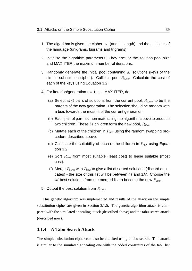
3.1. Attacks on the Simple Substitution Cipher 39
1. The algorithm is given the ciphertext (and its length) and the statistics ofthe language (unigrams, bigrams and trigrams).
2. Initialise the algorithm parameters. They are: M the solution pool sizeand MAX ITER the maximum number of iterations.
3. Randomly generate the initial pool containing M solutions (keys of thesimple substitution cipher). Call this pool PCURR. Calculate the cost ofeach of the keys using Equation 3.2.
4. For iteration/generation i = 1, . . . , MAX ITER, do
(a) Select M/2 pairs of solutions from the current pool, PCURR, to be theparents of the new generation. The selection should be random witha bias towards the most fit of the current generation.
(b) Each pair of parents then mate using the algorithm above to producetwo children. These M children form the new pool, PNEW.
(c) Mutate each of the children in PNEW using the random swapping pro-cedure described above.
(d) Calculate the suitability of each of the children in PNEW using Equa-tion 3.2.
(e) Sort PNEW from most suitable (least cost) to lease suitable (mostcost).
(f) Merge PCURR with PNEW to give a list of sorted solutions (discard dupli-cates) - the size of this list will be between M and 2M . Choose theM best solutions from the merged list to become the new PCURR.
5. Output the best solution from PCURR.
This genetic algorithm was implemented and results of the attack on the simple
substitution cipher are given in Section 3.1.5. The genetic algorithm attack is com-
pared with the simulated annealing attack (described above) and the tabu search attack
(described now).
3.1.4 A Tabu Search Attack
The simple substitution cipher can also be attacked using a tabu search. This attack
is similar to the simulated annealing one with the added constraints of the tabu list
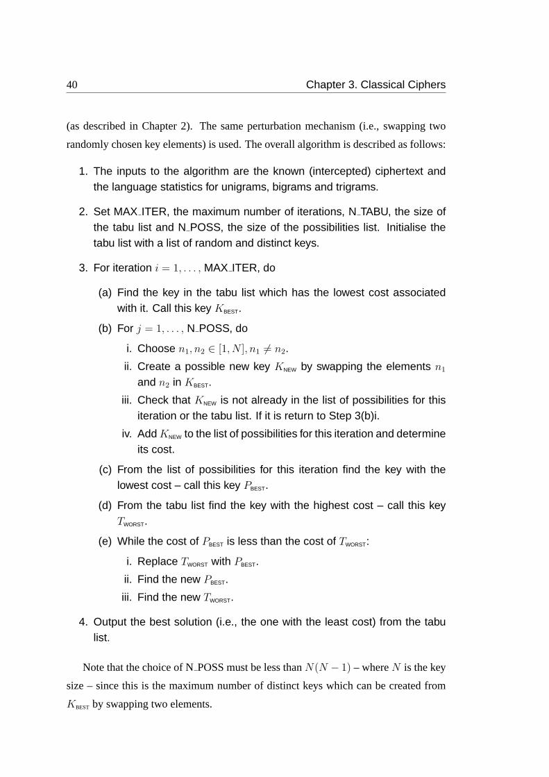
40 Chapter 3. Classical Ciphers
(as described in Chapter 2). The same perturbation mechanism (i.e., swapping two
randomly chosen key elements) is used. The overall algorithm is described as follows:
1. The inputs to the algorithm are the known (intercepted) ciphertext andthe language statistics for unigrams, bigrams and trigrams.
2. Set MAX ITER, the maximum number of iterations, N TABU, the size ofthe tabu list and N POSS, the size of the possibilities list. Initialise thetabu list with a list of random and distinct keys.
3. For iteration i = 1, . . . , MAX ITER, do
(a) Find the key in the tabu list which has the lowest cost associatedwith it. Call this key KBEST.
(b) For j = 1, . . . , N POSS, do
i. Choose n1, n2 ∈ [1, N ], n1 6= n2.
ii. Create a possible new key KNEW by swapping the elements n1
and n2 in KBEST.
iii. Check that KNEW is not already in the list of possibilities for thisiteration or the tabu list. If it is return to Step 3(b)i.
iv. Add KNEW to the list of possibilities for this iteration and determineits cost.
(c) From the list of possibilities for this iteration find the key with thelowest cost – call this key PBEST.
(d) From the tabu list find the key with the highest cost – call this keyTWORST.
(e) While the cost of PBEST is less than the cost of TWORST:
i. Replace TWORST with PBEST.
ii. Find the new PBEST.
iii. Find the new TWORST.
4. Output the best solution (i.e., the one with the least cost) from the tabulist.
Note that the choice of NPOSS must be less thanN(N − 1) – whereN is the key
size – since this is the maximum number of distinct keys which can be created from
KBEST by swapping two elements.
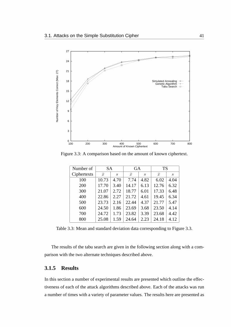
3.1. Attacks on the Simple Substitution Cipher 41
0
3
6
9
12
15
18
21
24
27
100 200 300 400 500 600 700 800
Num
ber
of K
ey E
lem
ents
Cor
rect
(M
ax: 2
7)
Amount of Known Ciphertext
Simulated AnnealingGenetic Algorithm
Tabu Search
Figure 3.3: A comparison based on the amount of known ciphertext.
Number of SA GA TSCiphertexts x s x s x s
100 10.73 4.70 7.74 4.82 6.02 4.04200 17.70 3.40 14.17 6.13 12.76 6.32300 21.07 2.72 18.77 6.01 17.33 6.48400 22.86 2.27 21.72 4.61 19.45 6.34500 23.73 2.16 22.44 4.37 21.77 5.47600 24.50 1.86 23.69 3.68 23.50 4.14700 24.72 1.73 23.82 3.39 23.68 4.42800 25.08 1.59 24.64 2.23 24.18 4.12
Table 3.3: Mean and standard deviation data corresponding to Figure 3.3.
The results of the tabu search are given in the following section along with a com-
parison with the two alternate techniques described above.
3.1.5 Results
In this section a number of experimental results are presented which outline the effec-
tiveness of each of the attack algorithms described above. Each of the attacks was run
a number of times with a variety of parameter values. The results here are presented as

42 Chapter 3. Classical Ciphers
0
3
6
9
12
15
18
21
24
27
0 5000 10000 15000 20000 25000 30000 35000
Num
ber
of K
ey E
lem
ents
Cor
rect
(M
ax: 2
7)
Total Keys Considered
Simulated AnnealingGenetic Algorithm
Tabu Search
Figure 3.4: A comparison based on the number of keys considered.
0
3
6
9
12
15
18
21
24
27
0 0.1 0.2 0.3 0.4 0.5 0.6 0.7
Num
ber
of K
ey E
lem
ents
Cor
rect
(M
ax: 2
7)
Time (seconds)
Simulated AnnealingGenetic Algorithm
Tabu Search
Figure 3.5: A comparison based on time.
plotted curves (Figures 3.3, 3.4 and 3.5). Each data point on these curves represents
three hundred runs of the particular algorithm. One hundred different messages were

3.1. Attacks on the Simple Substitution Cipher 43
generated in each case and the attack was run three times on each message. Of these
three runs on each message only the best result is considered. The numerical value
that is used in each of the plots is then the average over the one hundred messages of
the best result for each message. Why was this technique used? It is common when
using approximation algorithms to run the algorithm a number of times and then take
the best result. This is because of the random nature of the algorithms. By averaging
the results of a large number of independent attacks (in this case one hundred) a good
representation of the algorithm’s ability is obtained.
The first point to note is that each of the algorithms performed (approximately) as
well as the other with regard to the ultimate outcome of the attack. This is illustrated in
Figure 3.3 which compares the average number of key elements (out of 27) correctly
recovered versus the amount of ciphertext which is assumed known in the attack. The
plot shows results for amounts ranging from 100 to 800 known ciphertext characters.
In each case the results obtained are very similar for each of the algorithms. The mean,
x, and standard deviation values,s, for the results in Figure 3.3 are given in Table 3.3.
It can be seen that the standard deviation values for simulated annealing are less than
for the other two methods. This indicates that the simulated annealing approach, as
well as being slightly superior with respect to the mean values, has less variance in its
results.
Each of the algorithms perform roughly equally well when the comparison is made
based on the amount of ciphertext provided to the attack. It is interesting to make a
comparison based on the complexity of each of the attack algorithms. The remaining
results in this section aim to make a comparison of the algorithms based on complexity.
In each case, the following results were obtained using cryptograms of length 1000.
Figure 3.4 compares the number of correctly determined key elements with the total
number of keys considered up to that point by the algorithm. It is clear that the number
of keys considered by the simulated annealing technique in order to obtain the correct
key is significantly greater than for the other two techniques with the genetic algorithm
and the tabu search performing roughly equally in this respect. However, this com-
parison does not accurately indicate the relative efficiencies of the three algorithms.
In Figure 3.5, which compares the number of correct key elements discovered with
the amount of time used by the algorithm up to that point, it is clear that simulated
44 Chapter 3. Classical Ciphers
annealing is actually more efficient (with respect to time) that the genetic algorithm.
By comparing Figures 3.4 and 3.5 it can be concluded that the simulated annealing al-
gorithm is able to consider a far greater number of solutions that the genetic algorithm
and in much less time. It is also clear from both of these figures that the tabu search is
most efficient in both respects.
3.2 Attacks on Polyalphabetic Substitution Ciphers
The level of correspondence betweenn-gram statistics in the plaintext and ciphertext
messages for a polyalphabetic substitution cipher is not as high as for the simple sub-
stitution cipher, however, there is still a high enough correlation to achieve good results
in attacks. As can be observed from the encryption process, the frequency of single
characters (unigrams),for each block position, remains unchanged. Provided sufficient
ciphertext is obtained, it is possible to find a good approximation of the correct encryp-
tion keys, for each block position, simply by determining the unigram frequencies for
each block position. This, of course, assumes that the block length is known.
Methods for determining the block length were discussed in Section A.2. Another
method is now presented. This (ad hoc) technique for determining the period of a
polyalphabetic substitution cipher makes use of either a genetic algorithm or simulated
annealing. Matthews (in [47]) used a similar technique for finding key lengths of
transposition ciphers (see Section 3.3) with a genetic algorithm. The test procedure
involves running a genetic algorithm for a small number of generations with a fixed
block lengthB. This process is repeated for all potential values ofB (the correct
period). It is surmised that the cost of the best solution found for the correct period
will be significantly less than the best cost found for any of the incorrect periods. The
technique is described algorithmically as follows:
1. The inputs are the ciphertext and the required language statistics (un-igrams, bigrams and trigrams). It is presumed that the ciphertext wascreated using a polyalphabetic substitution cipher of unknown period.
2. For each of a series of possible period values:
(a) Run the attack (for example see the parallel genetic algorithm laterin this section) for a small number of iterations (say 20).
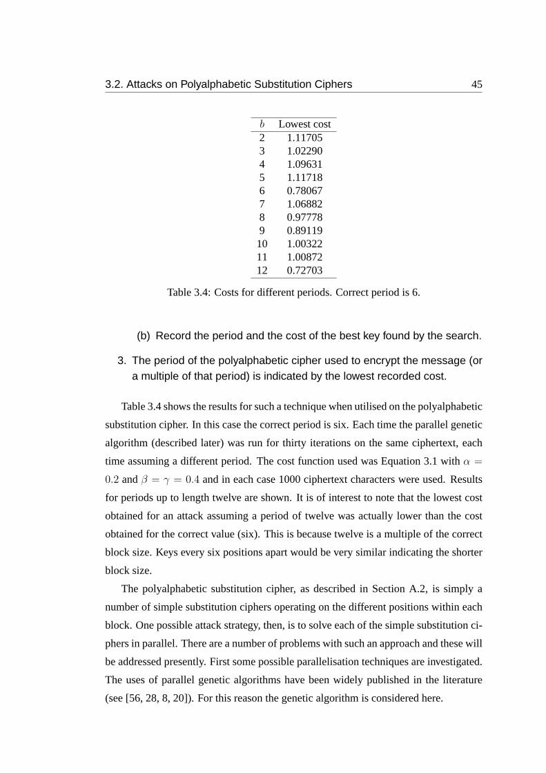
3.2. Attacks on Polyalphabetic Substitution Ciphers 45
b Lowest cost2 1.117053 1.022904 1.096315 1.117186 0.780677 1.068828 0.977789 0.8911910 1.0032211 1.0087212 0.72703
Table 3.4: Costs for different periods. Correct period is 6.
(b) Record the period and the cost of the best key found by the search.
3. The period of the polyalphabetic cipher used to encrypt the message (ora multiple of that period) is indicated by the lowest recorded cost.
Table 3.4 shows the results for such a technique when utilised on the polyalphabetic
substitution cipher. In this case the correct period is six. Each time the parallel genetic
algorithm (described later) was run for thirty iterations on the same ciphertext, each
time assuming a different period. The cost function used was Equation 3.1 withα =
0.2 andβ = γ = 0.4 and in each case 1000 ciphertext characters were used. Results
for periods up to length twelve are shown. It is of interest to note that the lowest cost
obtained for an attack assuming a period of twelve was actually lower than the cost
obtained for the correct value (six). This is because twelve is a multiple of the correct
block size. Keys every six positions apart would be very similar indicating the shorter
block size.
The polyalphabetic substitution cipher, as described in Section A.2, is simply a
number of simple substitution ciphers operating on the different positions within each
block. One possible attack strategy, then, is to solve each of the simple substitution ci-
phers in parallel. There are a number of problems with such an approach and these will
be addressed presently. First some possible parallelisation techniques are investigated.
The uses of parallel genetic algorithms have been widely published in the literature
(see [56, 28, 8, 20]). For this reason the genetic algorithm is considered here.

46 Chapter 3. Classical Ciphers
3.2.1 A Parallel Genetic Algorithm Attack
There are two broad ways in which a genetic algorithm can be parallelised. The first
is to parallelise the selection, mating and mutation phases in the genetic algorithm.
Such a technique can be used to enhance almost any implementation of the genetic
algorithm. Figure 3.6 illustrates this idea.
New Generation
Children
Parents
Current Generation
Selection
Mate
Mutation
Figure 3.6: A parallel heuristic for any genetic algorithm.
When designing parallel heuristics one must be aware of the time overhead asso-
ciated with transporting data to and from separate processing nodes. The heuristic
presented in Figure 3.6 is only useful when dedicated hardware is available which can
perform the necessary functions (eg., selection, mating, mutation and fitness/cost de-
termination). Typically the complexity of each of these individual functions is very
small, however a large number of processing nodes are required in order to gain ad-
vantage from the parallel architecture of the algorithm.
An alternative heuristic is to have a number of genetic algorithms running in paral-
lel, each solving a different part of the problem. Figure 3.7 is a pictorial representation
of this strategy withM GA’s running in parallel and communicating everyk itera-
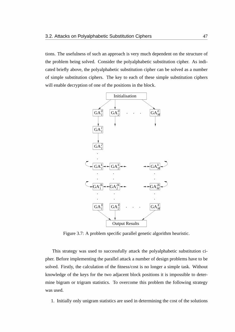
3.2. Attacks on Polyalphabetic Substitution Ciphers 47
tions. The usefulness of such an approach is very much dependent on the structure of
the problem being solved. Consider the polyalphabetic substitution cipher. As indi-
cated briefly above, the polyalphabetic substitution cipher can be solved as a number
of simple substitution ciphers. The key to each of these simple substitution ciphers
will enable decryption of one of the positions in the block.
GAMX
GAM2kGA2
2kGA12k
GA1k kGA2 GAM
k
XGA2GA1X
GA12
GA11
GA10 0GA2 GA0
M
Initialisation
Output Results
. . .
.
.
.
...
.
.
.
.
. . .
.
...
Figure 3.7: A problem specific parallel genetic algorithm heuristic.
This strategy was used to successfully attack the polyalphabetic substitution ci-
pher. Before implementing the parallel attack a number of design problems have to be
solved. Firstly, the calculation of the fitness/cost is no longer a simple task. Without
knowledge of the keys for the two adjacent block positions it is impossible to deter-
mine bigram or trigram statistics. To overcome this problem the following strategy
was used.
1. Initially only unigram statistics are used in determining the cost of the solutions
48 Chapter 3. Classical Ciphers
in any pool.
2. Everyx iterations of each GA, the most fit solution in the current pool is sent to
each of the neighbouring GA’s. Each GA has knowledge of the entire ciphertext
message so it is able to determine a fitness based on unigram, bigram and trigram
statistics using ciphertext characters in its position, the position to the left and
the position to the right.
In an attempt to illustrate more clearly the description of the previous paragraph
the following symbolic outline is given. Consider a polyalphabetic substitution cipher
consisting ofB monoalphabetic or simple substitution ciphers. There will then be
B genetic algorithms (call them GA1, GA2, . . . , GAB) solving each of theB simple
substitution ciphers. Now consider GAj (1 < j < B) which is attempting to find the
key to the cipher of positionj. In determining the cost of each of the solutions in its
pool, GAj uses the current best key from each of its neighbours to find the bigram and
trigram statistics.
The second problem to be solved when implementing a parallel GA is to determine
how the different GA’s will communicate between each another. The work presented
here makes use of a software package called PVM (Parallel Virtual Machine) [62]
which enables a number of networked computers to be linked as a virtual parallel
computer in which a single application can be spread across a number of different
physical computers. The use of such a package allows each of the individual GA’s to
communicate by sending the neighbours its current best keys.
With these design problems solved the implementation of each genetic algorithm
proceeds as follows.
1. Each GA is given language statistics for unigrams, bigrams and trigrams,the ciphertext, the block size (B) and this GA’s position within the block, j
(1 ≤ j ≤ B), the frequency of inter-GA communications (f ), the maximumnumber of iterations for the GA (G) and the solution pool size (M ).
2. Generate a random pool of M simple substitution cipher keys for positionj and calculate the cost for each using unigram statistics only. Call thispool of solutions PCURR.
3. For iteration/generation i (i = 1, . . . , G) do:
3.2. Attacks on Polyalphabetic Substitution Ciphers 49
(a) If i mod k ≡ 0 send the best key from PCURR to each of the neighbour-ing GA’s (i.e., the GA’s solving for positions j − 1 and j + 1). Alsoreceive the best keys from each of these GA’s.
(b) Select M/2 pairs of solutions from PCURR to be the parents of the newgeneration. The selection should be biased towards the most fit ofthe current generation (i.e., the keys in PCURR).
(c) Mate using each pair of parents with the algorithm given above. Thisproduces M children which become the new generation (i.e., thesolutions of PNEW).
(d) Mutate each of the children in PNEW using the same swapping proce-dure as described in the attack on the simple substitution cipher.
(e) Calculate the cost of each of the children in PNEW using the neigh-bouring keys obtained in Step 3a and Equation 3.1.
(f) Select the M best keys from the two pools PCURR and PNEW. Replacethe current solutions in PCURR with these solutions.
4. Output the best key from PCURR.
Experimental results obtained from this algorithm are now given. It is shown that
the parallel technique is effective for polyalphabetic substitution ciphers with a variety
of block sizes.
3.2.2 Results
It is clear that the parallel implementation of the attack will perform much more effi-
ciently than a serial version since the parallel attack is solving each key of the polyal-
phabetic cipher simultaneously. The overhead of communication between the parallel
processors is minimal leading to an attack of the polyalphabetic substitution cipher
which would be expected to complete in roughly the same time as a similar attack on
a monoalphabetic substitution cipher. In this section results based on the amount of
ciphertext provided to the attack are given. These results can be compared with those
obtained in Figure 3.3 for the simple substitution cipher.
The algorithm described above was implemented using a public domain software
package called PVM (Parallel Virtual Machine) [62] which allows the development of
parallel applications by sharing the processors of a number of networked computers (or
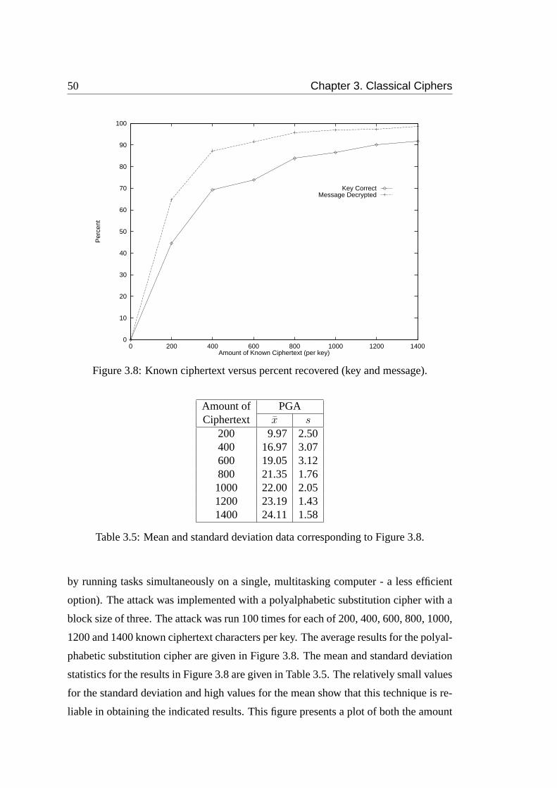
50 Chapter 3. Classical Ciphers
0
10
20
30
40
50
60
70
80
90
100
0 200 400 600 800 1000 1200 1400
Per
cent
Amount of Known Ciphertext (per key)
Key CorrectMessage Decrypted
Figure 3.8: Known ciphertext versus percent recovered (key and message).
Amount of PGACiphertext x s
200 9.97 2.50400 16.97 3.07600 19.05 3.12800 21.35 1.761000 22.00 2.051200 23.19 1.431400 24.11 1.58
Table 3.5: Mean and standard deviation data corresponding to Figure 3.8.
by running tasks simultaneously on a single, multitasking computer - a less efficient
option). The attack was implemented with a polyalphabetic substitution cipher with a
block size of three. The attack was run 100 times for each of 200, 400, 600, 800, 1000,
1200 and 1400 known ciphertext characters per key. The average results for the polyal-
phabetic substitution cipher are given in Figure 3.8. The mean and standard deviation
statistics for the results in Figure 3.8 are given in Table 3.5. The relatively small values
for the standard deviation and high values for the mean show that this technique is re-
liable in obtaining the indicated results. This figure presents a plot of both the amount
3.3. Attacks on Transposition Ciphers 51
of message recovered and the amount of key recovered as a percentage. Recall that
for the simple substitution cipher (see Figure 3.3) that roughly 25 out of 27 key ele-
ments were correctly recovered after approximately 800 known ciphertext characters
were provided. The parallel genetic algorithm attack of the polyalphabetic substitution
cipher required about 1400 characters per key to obtain a similar result. This is to
be expected because of the reduced number of trigrams available to the attack on the
polyalphabetic substitution cipher.
The parallel algorithm was run on block sizes (B) ranging from 3 to 9. In each case
there were 1500 characters of ciphertextper key. It was found that, regardless of block
size, the algorithm was able to fully recover at least 99% of the original message. This
result was obtained by running the algorithm using 100 different ciphertext messages
for each block size and averaging the number of correctly placed key elements in each
case. In each case the average number of key elements correctly placed was more than
26 out of 27 for each position in the block.
These results indicate that the parallel genetic algorithm is an extremely powerful
technique for attacks on polyalphabetic substitution ciphers. It could be surmised from
the experimental results given above that the attack could be used on polyalphabetic ci-
phers with very large periods provided that sufficient ciphertext and a parallel machine
with sufficient nodes to implement the attack are available to the cryptanalyst.
3.3 Attacks on Transposition Ciphers
In this section three techniques are presented which can be utilised in attacks on the
transposition cipher. These techniques make use of simulated annealing, the genetic
algorithm and the tabu search, respectively. Recall that the attacks on the substitution
ciphers used a perturbation mechanism which simply swapped two randomly chosen
elements of the key. An additional mechanism is used in the attacks on the transposi-
tion cipher. This mechanism rotates a random (but consecutive) subsection of the key
by a random amount. Possible cost functions for the attacks on the transposition cipher
are now discussed.
52 Chapter 3. Classical Ciphers
3.3.1 Suitability Assessment
It is possible to use exactly the same cost to evaluate a key of a transposition cipher
as the one used in Equation 3.1 for the simple substitution cipher. In the process of
determining the cost associated with a transposition cipher key the proposed key is
used to decrypt the ciphertext and then the statistics of the decrypted message are then
compared with statistics of the language.
Matthews, in [47], proposed an intuitive (but never-the-less clever) alternative. In-
stead of using all possible bigrams and trigrams a subset of the most common ones are
chosen. (Remember unigram frequencies are unchanged during the encryption process
and so are ignored when evaluating a key.)
The method Matthews used was to list a number of the most common bigrams
and trigrams and to assign a weight (or score) to each of them. Also, the trigram
“EEE” was included in the list and assigned a negative score. The idea behind this is
interesting. SinceE is very common in English, it could be expected that a plaintext
message might contain a relatively high number ofE’s. The same frequency ofE’s will
be present in the ciphertext, but, in this case, it could be expected that, on occasion,
threeE’s might occur simultaneously. Since these never occur normally in th English
language, it makes sense to assign such a trigram a negative score.
Each weight is applied to the frequency of the corresponding bigram or trigram
in the decrypted message. Note that Matthews’ method (in [47]) was expressed in
terms of a fitness function so the negative weight assigned to the trigram “___ ” (three
consecutive spaces) had the effect of reducing the fitness. Table 3.6 shows the weight
table used by Matthews in his paper. The bigrams, trigrams and weights were modified
for the research in this thesis to the values shown in Table 3.7. Notice that the bigram
“__” (two consecutive spaces) and the trigram “___ ” (three consecutive spaces) have
been included. Some of the other bigrams and trigrams are slightly different - due to
the fact that the space symbol has been included in the encryption in this work (and
was not in the work by Matthews) and also (perhaps) due to different sets of language
statistics being used.
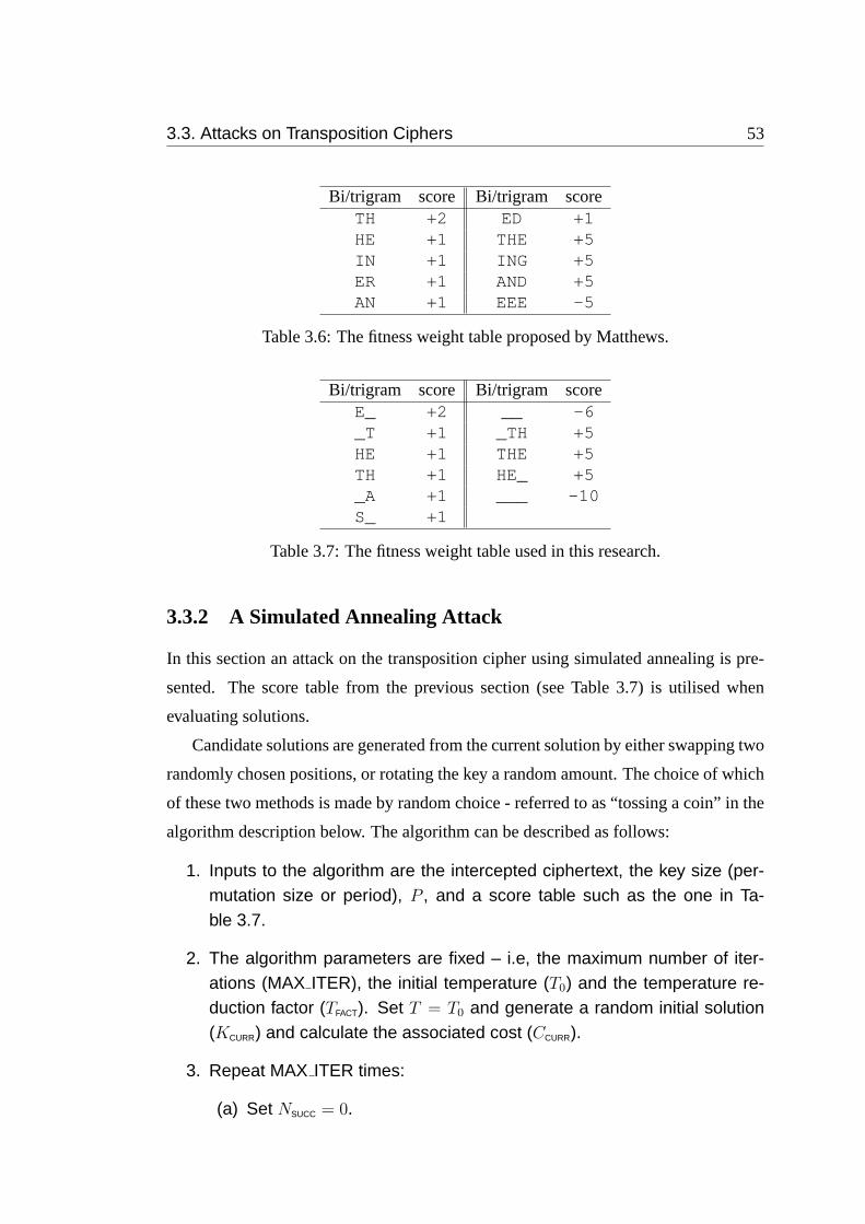
3.3. Attacks on Transposition Ciphers 53
Bi/trigram score Bi/trigram scoreTH +2 ED +1HE +1 THE +5IN +1 ING +5ER +1 AND +5AN +1 EEE -5
Table 3.6: The fitness weight table proposed by Matthews.
Bi/trigram score Bi/trigram scoreE_ +2 __ -6_T +1 _TH +5HE +1 THE +5TH +1 HE_ +5_A +1 ___ -10S_ +1
Table 3.7: The fitness weight table used in this research.
3.3.2 A Simulated Annealing Attack
In this section an attack on the transposition cipher using simulated annealing is pre-
sented. The score table from the previous section (see Table 3.7) is utilised when
evaluating solutions.
Candidate solutions are generated from the current solution by either swapping two
randomly chosen positions, or rotating the key a random amount. The choice of which
of these two methods is made by random choice - referred to as “tossing a coin” in the
algorithm description below. The algorithm can be described as follows:
1. Inputs to the algorithm are the intercepted ciphertext, the key size (per-mutation size or period), P , and a score table such as the one in Ta-ble 3.7.
2. The algorithm parameters are fixed – i.e, the maximum number of iter-ations (MAX ITER), the initial temperature (T0) and the temperature re-duction factor (TFACT). Set T = T0 and generate a random initial solution(KCURR) and calculate the associated cost (CCURR).
3. Repeat MAX ITER times:
(a) Set NSUCC = 0.
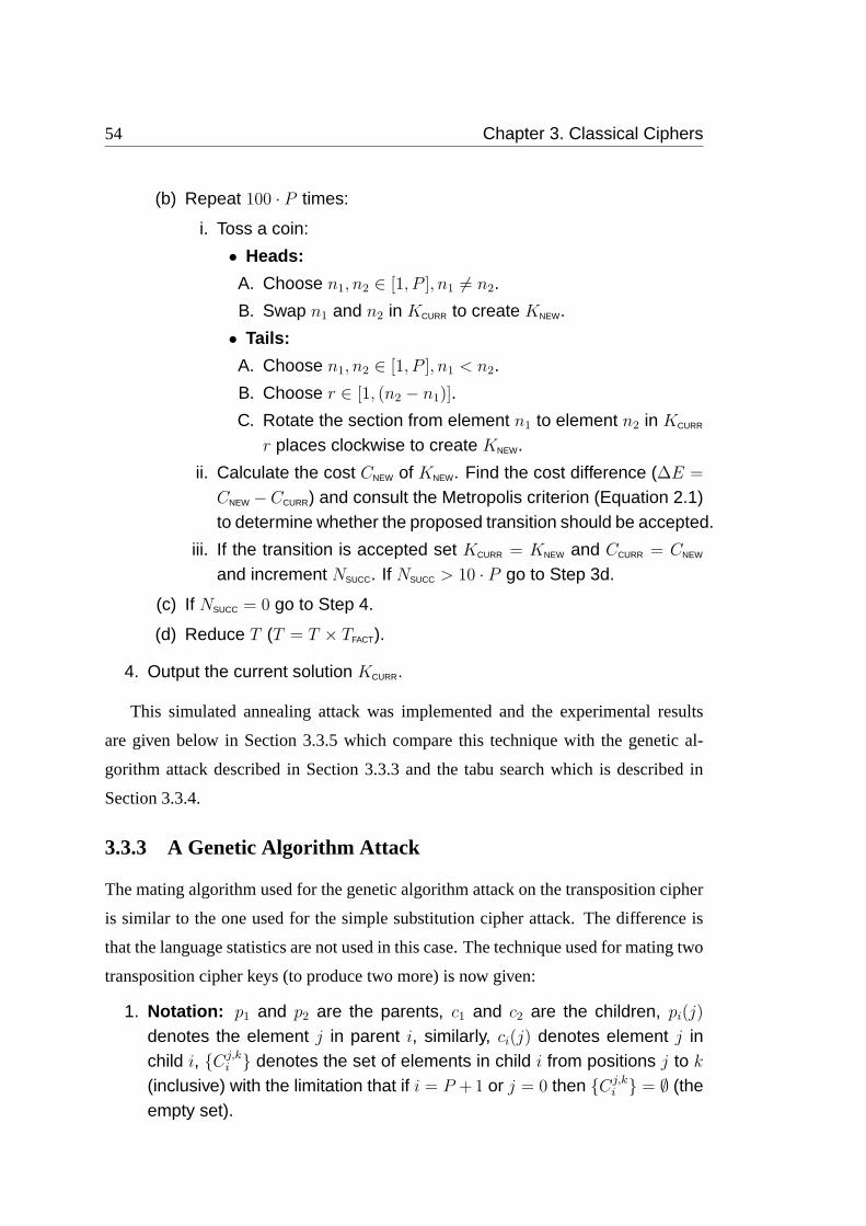
54 Chapter 3. Classical Ciphers
(b) Repeat 100 · P times:
i. Toss a coin:
• Heads:
A. Choose n1, n2 ∈ [1, P ], n1 6= n2.
B. Swap n1 and n2 in KCURR to create KNEW.
• Tails:
A. Choose n1, n2 ∈ [1, P ], n1 < n2.
B. Choose r ∈ [1, (n2 − n1)].
C. Rotate the section from element n1 to element n2 in KCURR
r places clockwise to create KNEW.
ii. Calculate the cost CNEW of KNEW. Find the cost difference (∆E =
CNEW −CCURR) and consult the Metropolis criterion (Equation 2.1)to determine whether the proposed transition should be accepted.
iii. If the transition is accepted set KCURR = KNEW and CCURR = CNEW
and increment NSUCC. If NSUCC > 10 · P go to Step 3d.
(c) If NSUCC = 0 go to Step 4.
(d) Reduce T (T = T × TFACT).
4. Output the current solution KCURR.
This simulated annealing attack was implemented and the experimental results
are given below in Section 3.3.5 which compare this technique with the genetic al-
gorithm attack described in Section 3.3.3 and the tabu search which is described in
Section 3.3.4.
3.3.3 A Genetic Algorithm Attack
The mating algorithm used for the genetic algorithm attack on the transposition cipher
is similar to the one used for the simple substitution cipher attack. The difference is
that the language statistics are not used in this case. The technique used for mating two
transposition cipher keys (to produce two more) is now given:
1. Notation: p1 and p2 are the parents, c1 and c2 are the children, pi(j)
denotes the element j in parent i, similarly, ci(j) denotes element j inchild i, {Cj,k
i } denotes the set of elements in child i from positions j to k
(inclusive) with the limitation that if i = P +1 or j = 0 then {Cj,ki } = ∅ (the
empty set).
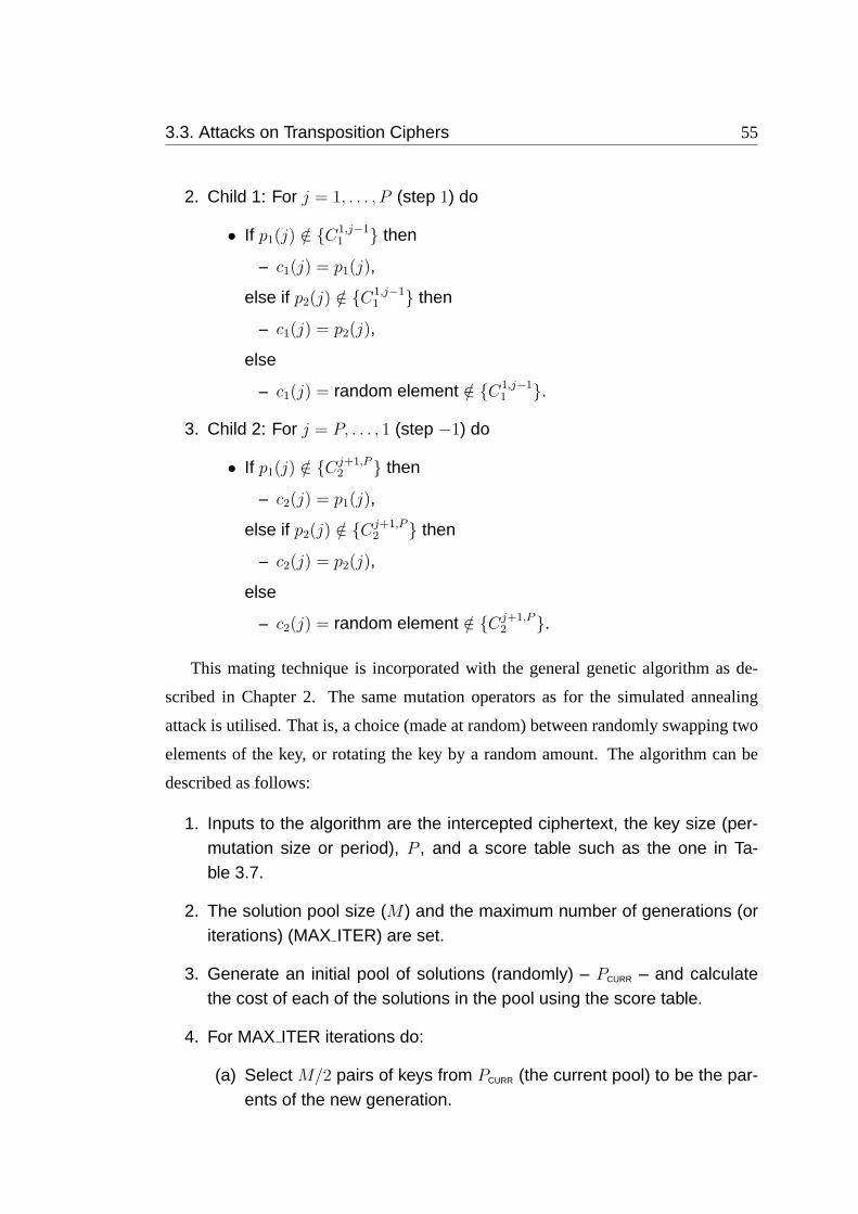
3.3. Attacks on Transposition Ciphers 55
2. Child 1: For j = 1, . . . , P (step 1) do
• If p1(j) /∈ {C1,j−11 } then
– c1(j) = p1(j),
else if p2(j) /∈ {C1,j−11 } then
– c1(j) = p2(j),
else
– c1(j) = random element /∈ {C1,j−11 }.
3. Child 2: For j = P, . . . , 1 (step −1) do
• If p1(j) /∈ {Cj+1,P2 } then
– c2(j) = p1(j),
else if p2(j) /∈ {Cj+1,P2 } then
– c2(j) = p2(j),
else
– c2(j) = random element /∈ {Cj+1,P2 }.
This mating technique is incorporated with the general genetic algorithm as de-
scribed in Chapter 2. The same mutation operators as for the simulated annealing
attack is utilised. That is, a choice (made at random) between randomly swapping two
elements of the key, or rotating the key by a random amount. The algorithm can be
described as follows:
1. Inputs to the algorithm are the intercepted ciphertext, the key size (per-mutation size or period), P , and a score table such as the one in Ta-ble 3.7.
2. The solution pool size (M ) and the maximum number of generations (oriterations) (MAX ITER) are set.
3. Generate an initial pool of solutions (randomly) – PCURR – and calculatethe cost of each of the solutions in the pool using the score table.
4. For MAX ITER iterations do:
(a) Select M/2 pairs of keys from PCURR (the current pool) to be the par-ents of the new generation.
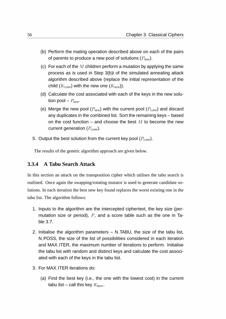
56 Chapter 3. Classical Ciphers
(b) Perform the mating operation described above on each of the pairsof parents to produce a new pool of solutions (PNEW).
(c) For each of the M children perform a mutation by applying the sameprocess as is used in Step 3(b)i of the simulated annealing attackalgorithm described above (replace the initial representation of thechild (KCURR) with the new one (KNEW)).
(d) Calculate the cost associated with each of the keys in the new solu-tion pool – PNEW.
(e) Merge the new pool (PNEW) with the current pool (PCURR) and discardany duplicates in the combined list. Sort the remaining keys – basedon the cost function – and choose the best M to become the newcurrent generation (PCURR).
5. Output the best solution from the current key pool (PCURR).
The results of the genetic algorithm approach are given below.
3.3.4 A Tabu Search Attack
In this section an attack on the transposition cipher which utilises the tabu search is
outlined. Once again the swapping/rotating mutator is used to generate candidate so-
lutions. In each iteration the best new key found replaces the worst existing one in the
tabu list. The algorithm follows:
1. Inputs to the algorithm are the intercepted ciphertext, the key size (per-mutation size or period), P , and a score table such as the one in Ta-ble 3.7.
2. Initialise the algorithm parameters – N TABU, the size of the tabu list,N POSS, the size of the list of possibilities considered in each iterationand MAX ITER, the maximum number of iterations to perform. Initialisethe tabu list with random and distinct keys and calculate the cost associ-ated with each of the keys in the tabu list.
3. For MAX ITER iterations do:
(a) Find the best key (i.e., the one with the lowest cost) in the currenttabu list – call this key KBEST.
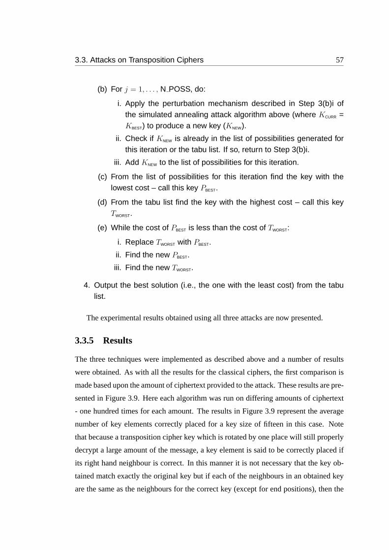
3.3. Attacks on Transposition Ciphers 57
(b) For j = 1, . . . , N POSS, do:
i. Apply the perturbation mechanism described in Step 3(b)i ofthe simulated annealing attack algorithm above (where KCURR =KBEST) to produce a new key (KNEW).
ii. Check if KNEW is already in the list of possibilities generated forthis iteration or the tabu list. If so, return to Step 3(b)i.
iii. Add KNEW to the list of possibilities for this iteration.
(c) From the list of possibilities for this iteration find the key with thelowest cost – call this key PBEST.
(d) From the tabu list find the key with the highest cost – call this keyTWORST.
(e) While the cost of PBEST is less than the cost of TWORST:
i. Replace TWORST with PBEST.
ii. Find the new PBEST.
iii. Find the new TWORST.
4. Output the best solution (i.e., the one with the least cost) from the tabulist.
The experimental results obtained using all three attacks are now presented.
3.3.5 Results
The three techniques were implemented as described above and a number of results
were obtained. As with all the results for the classical ciphers, the first comparison is
made based upon the amount of ciphertext provided to the attack. These results are pre-
sented in Figure 3.9. Here each algorithm was run on differing amounts of ciphertext
- one hundred times for each amount. The results in Figure 3.9 represent the average
number of key elements correctly placed for a key size of fifteen in this case. Note
that because a transposition cipher key which is rotated by one place will still properly
decrypt a large amount of the message, a key element is said to be correctly placed if
its right hand neighbour is correct. In this manner it is not necessary that the key ob-
tained match exactly the original key but if each of the neighbours in an obtained key
are the same as the neighbours for the correct key (except for end positions), then the
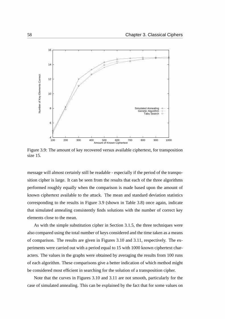
58 Chapter 3. Classical Ciphers
4
6
8
10
12
14
16
100 200 300 400 500 600 700 800 900 1000
Num
ber
of K
ey E
lem
ents
Cor
rect
Amount of Known Ciphertext
Simulated AnnealingGenetic Algorithm
Tabu Search
Figure 3.9: The amount of key recovered versus available ciphertext, for transpositionsize 15.
message will almost certainly still be readable - especially if the period of the transpo-
sition cipher is large. It can be seen from the results that each of the three algorithms
performed roughly equally when the comparison is made based upon the amount of
known ciphertext available to the attack. The mean and standard deviation statistics
corresponding to the results in Figure 3.9 (shown in Table 3.8) once again, indicate
that simulated annealing consistently finds solutions with the number of correct key
elements close to the mean.
As with the simple substitution cipher in Section 3.1.5, the three techniques were
also compared using the total number of keys considered and the time taken as a means
of comparison. The results are given in Figures 3.10 and 3.11, respectively. The ex-
periments were carried out with a period equal to 15 with 1000 known ciphertext char-
acters. The values in the graphs were obtained by averaging the results from 100 runs
of each algorithm. These comparisons give a better indication of which method might
be considered most efficient in searching for the solution of a transposition cipher.
Note that the curves in Figures 3.10 and 3.11 are not smooth, particularly for the
case of simulated annealing. This can be explained by the fact that for some values on
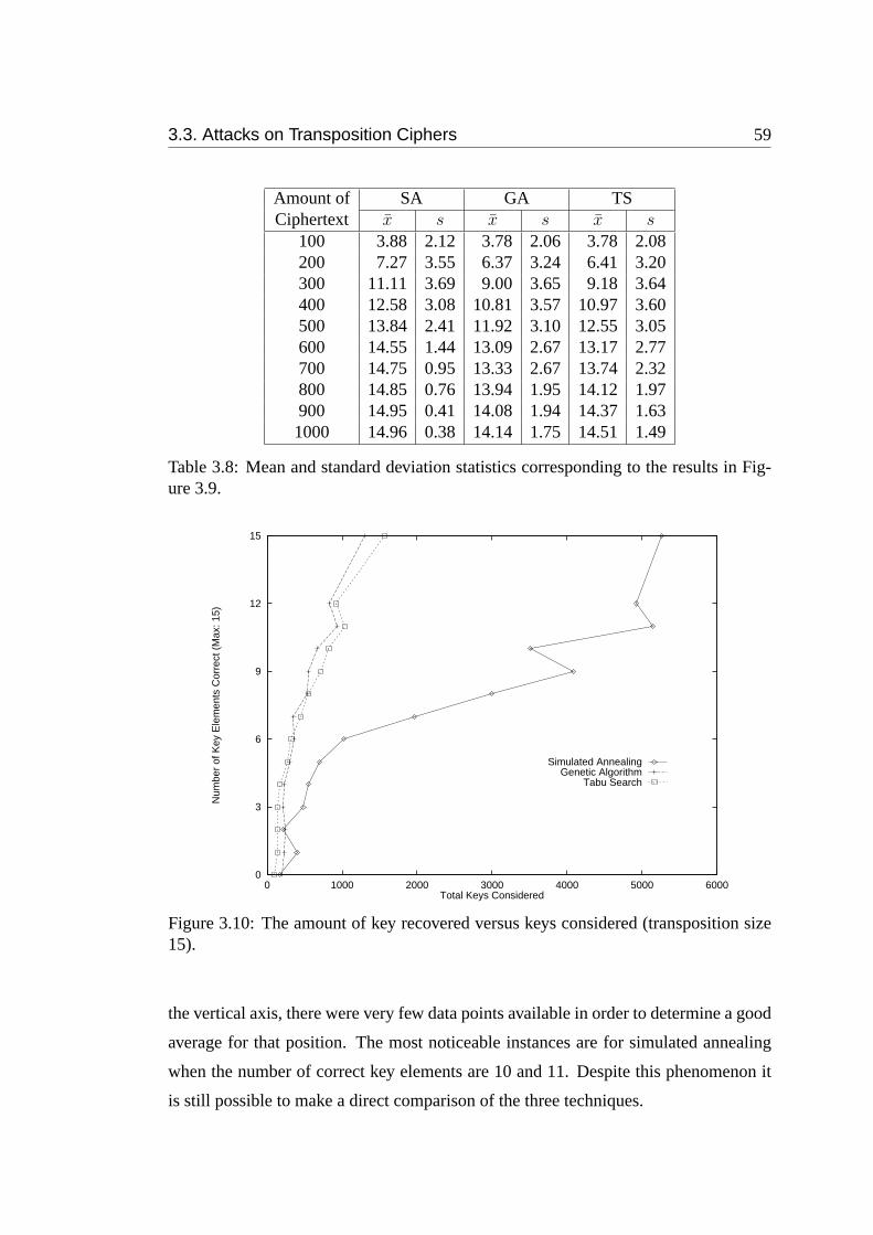
3.3. Attacks on Transposition Ciphers 59
Amount of SA GA TSCiphertext x s x s x s
100 3.88 2.12 3.78 2.06 3.78 2.08200 7.27 3.55 6.37 3.24 6.41 3.20300 11.11 3.69 9.00 3.65 9.18 3.64400 12.58 3.08 10.81 3.57 10.97 3.60500 13.84 2.41 11.92 3.10 12.55 3.05600 14.55 1.44 13.09 2.67 13.17 2.77700 14.75 0.95 13.33 2.67 13.74 2.32800 14.85 0.76 13.94 1.95 14.12 1.97900 14.95 0.41 14.08 1.94 14.37 1.631000 14.96 0.38 14.14 1.75 14.51 1.49
Table 3.8: Mean and standard deviation statistics corresponding to the results in Fig-ure 3.9.
0
3
6
9
12
15
0 1000 2000 3000 4000 5000 6000
Num
ber
of K
ey E
lem
ents
Cor
rect
(M
ax: 1
5)
Total Keys Considered
Simulated AnnealingGenetic Algorithm
Tabu Search
Figure 3.10: The amount of key recovered versus keys considered (transposition size15).
the vertical axis, there were very few data points available in order to determine a good
average for that position. The most noticeable instances are for simulated annealing
when the number of correct key elements are 10 and 11. Despite this phenomenon it
is still possible to make a direct comparison of the three techniques.
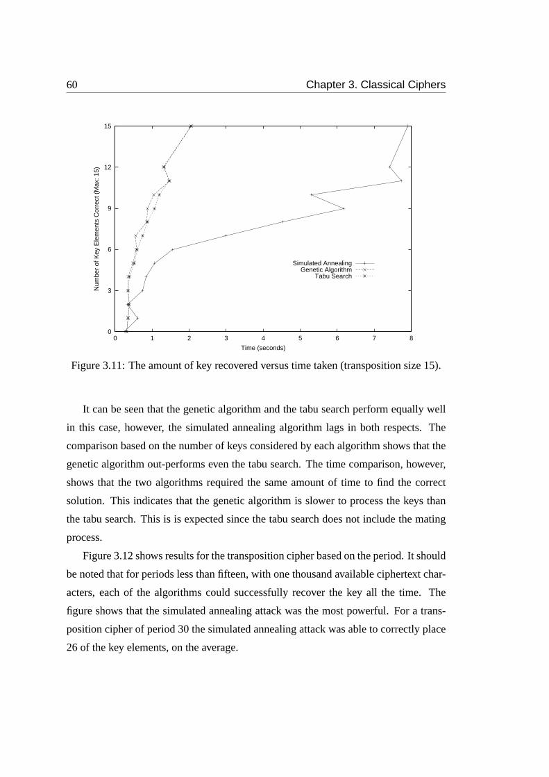
60 Chapter 3. Classical Ciphers
0
3
6
9
12
15
0 1 2 3 4 5 6 7 8
Num
ber
of K
ey E
lem
ents
Cor
rect
(M
ax: 1
5)
Time (seconds)
Simulated AnnealingGenetic Algorithm
Tabu Search
Figure 3.11: The amount of key recovered versus time taken (transposition size 15).
It can be seen that the genetic algorithm and the tabu search perform equally well
in this case, however, the simulated annealing algorithm lags in both respects. The
comparison based on the number of keys considered by each algorithm shows that the
genetic algorithm out-performs even the tabu search. The time comparison, however,
shows that the two algorithms required the same amount of time to find the correct
solution. This indicates that the genetic algorithm is slower to process the keys than
the tabu search. This is is expected since the tabu search does not include the mating
process.
Figure 3.12 shows results for the transposition cipher based on the period. It should
be noted that for periods less than fifteen, with one thousand available ciphertext char-
acters, each of the algorithms could successfully recover the key all the time. The
figure shows that the simulated annealing attack was the most powerful. For a trans-
position cipher of period 30 the simulated annealing attack was able to correctly place
26 of the key elements, on the average.
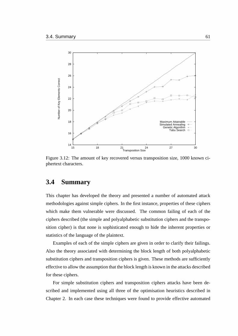
3.4. Summary 61
14
16
18
20
22
24
26
28
30
15 18 21 24 27 30
Num
ber
of K
ey E
lem
ents
Cor
rect
Transposition Size
Maximum AttainableSimulated Annealing
Genetic AlgorithmTabu Search
Figure 3.12: The amount of key recovered versus transposition size, 1000 known ci-phertext characters.
3.4 Summary
This chapter has developed the theory and presented a number of automated attack
methodologies against simple ciphers. In the first instance, properties of these ciphers
which make them vulnerable were discussed. The common failing of each of the
ciphers described (the simple and polyalphabetic substitution ciphers and the transpo-
sition cipher) is that none is sophisticated enough to hide the inherent properties or
statistics of the language of the plaintext.
Examples of each of the simple ciphers are given in order to clarify their failings.
Also the theory associated with determining the block length of both polyalphabetic
substitution ciphers and transposition ciphers is given. These methods are sufficiently
effective to allow the assumption that the block length is known in the attacks described
for these ciphers.
For simple substitution ciphers and transposition ciphers attacks have been de-
scribed and implemented using all three of the optimisation heuristics described in
Chapter 2. In each case these techniques were found to provide effective automated
62 Chapter 3. Classical Ciphers
techniques for the cryptanalysis of the ciphertext. Provided sufficient ciphertext is in-
tercepted by an attacker, each of these algorithms will provide enough information to
make the plaintext message understandable.
Comparisons of the three techniques were also made based on the number of keys
considered and the time taken by the algorithm. It was found that for the simple substi-
tution cipher the tabu search out-performed both simulated annealing and the genetic
algorithm with simulated annealing taking roughly twice as long as the tabu search
and the genetic algorithm taking roughly twice as long as simulated annealing. These
results differed for the transposition cipher where the tabu search and the genetic al-
gorithm performed equally well and roughly four times faster than the simulated an-
nealing attack. However, the simulated annealing attack on the transposition cipher
performed better than the other two techniques on large transposition sizes.
A parallel heuristic for the genetic algorithm is presented along with an associ-
ated algorithm for the cryptanalysis of the polyalphabetic substitution cipher. It is
shown that this algorithm also gives an accurate indication of the block length used
in the encryption process. A parallel technique is desirable considering the efficiency
gains obtained from such an approach. The attack described in this chapter effec-
tively reduces the complexity of a polyalphabetic substitution cipher attack to that of a
monoalphabetic one (provided a computer withB processing nodes is available).
Overall, optimisation heuristics are ideally suited to implementations in attacks on
the classic ciphers. This has been shown by the experimental results in the chapter.
The remainder of this dissertation deals with different applications of optimisation
heuristics in the fields of cryptanalysis and cryptography.
Chapter 4
Attacks on a Certain Class of StreamCiphers
In this chapter a number of techniques for the cryptanalysis of a certain class of stream
cipher are presented. In the most commonly used stream ciphers a pseudo-random
sequence of bits is combined (using modulo 2 addition, or XOR) with the plaintext
to produce the ciphertext. The class of stream ciphers being considered here produce
a pseudo-random output sequence by the nonlinear combination of the output of a
number of linear feedback shift register (LFSR) sequences. A general overview of the
LFSR and LFSR-based stream ciphers is given in Appendix B.
Attacks on this class of stream cipher are well known. Meier and Staffelbach [48]
and Zeng and Huang [78] are considered the pioneers of attacks on these ciphers.
Subsequent to their research, a number of publications appeared which theoretically
and experimentally analysed these and other similar attacks (for example, see [10, 54,
55]). All of these techniques have two features in common: an iterative error correction
algorithm and a method of obtaining low density parity checks. The fast correlation
attack (FCA) introduced by Meier and Staffelbach [48] uses a probability vector and
Bayesian bit-by-bit error correction in order to recover the initial LFSR contents. All of
the attacks considered in this chapter have as their goal the task of recovering the initial
contents (orseeds) of the LFSR’s using less effort than is required by an exhaustive
search.
The fast correlation attack, as proposed by Meier and Staffelbach [48] is described
in Section 4.1. This description includes discussion of the probabilistic model used by
the attack as well as the concept of parity checks which are central to the algorithm.
63
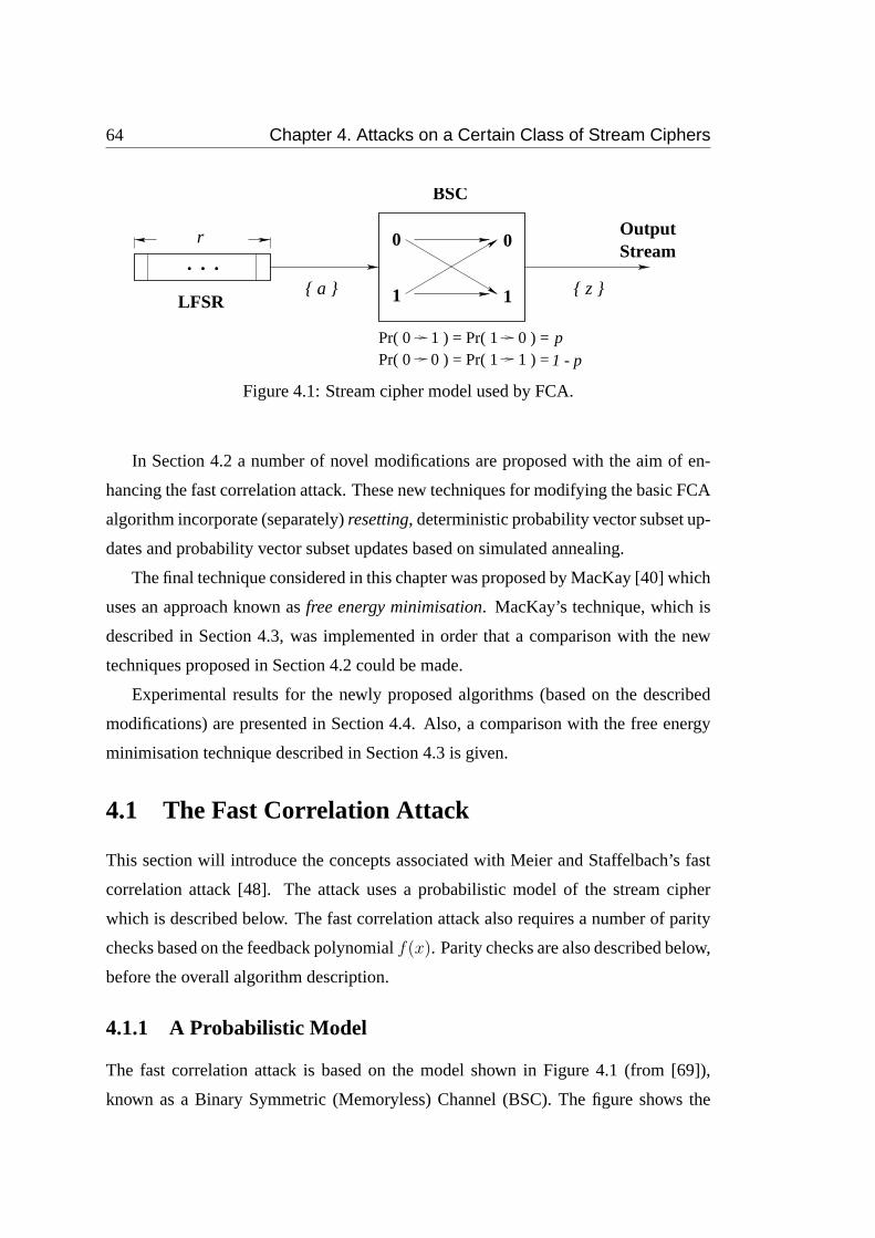
64 Chapter 4. Attacks on a Certain Class of Stream Ciphers
. . .r
{ a } { z }LFSR
0
1 1
0
Pr( 0 1 ) = Pr( 1 0 ) =Pr( 0 0 ) = Pr( 1 1 ) =
BSC
StreamOutput
p
1 - p
Figure 4.1: Stream cipher model used by FCA.
In Section 4.2 a number of novel modifications are proposed with the aim of en-
hancing the fast correlation attack. These new techniques for modifying the basic FCA
algorithm incorporate (separately)resetting, deterministic probability vector subset up-
dates and probability vector subset updates based on simulated annealing.
The final technique considered in this chapter was proposed by MacKay [40] which
uses an approach known asfree energy minimisation. MacKay’s technique, which is
described in Section 4.3, was implemented in order that a comparison with the new
techniques proposed in Section 4.2 could be made.
Experimental results for the newly proposed algorithms (based on the described
modifications) are presented in Section 4.4. Also, a comparison with the free energy
minimisation technique described in Section 4.3 is given.
4.1 The Fast Correlation Attack
This section will introduce the concepts associated with Meier and Staffelbach’s fast
correlation attack [48]. The attack uses a probabilistic model of the stream cipher
which is described below. The fast correlation attack also requires a number of parity
checks based on the feedback polynomialf(x). Parity checks are also described below,
before the overall algorithm description.
4.1.1 A Probabilistic Model
The fast correlation attack is based on the model shown in Figure 4.1 (from [69]),
known as a Binary Symmetric (Memoryless) Channel (BSC). The figure shows the
4.1. The Fast Correlation Attack 65
output key stream to be represented as a noise-corrupted version of the output of one
of the LFSR’s. The LFSR sequence is denoteda = {ai}Ni=1 and the output keystream
sequence is denotedz = {zi}Ni=1. Thuszi = ai ⊕ ei, wheree = {ei}N
i=1 is a binary
noise sequence with the noise probabilityp defined by Pr(ei = 1) = p (i = 1, . . . , N ).
The LFSR is defined by the feedback polynomialf(x) which is assumed known by
the attacker. Let the length of the LFSR be denotedr. The aim of the attack is to
reconstruct the LFSR output sequence,a = {ai}Ni=1, given the output keystream,z =
{zi},Ni=1, with the restriction thatN , the length of the keystream sequence, be as small
as possible, but in the boundsr < N < 2r − 1.
4.1.2 Parity Checks
Central to understanding the fast correlation attack is the concept of a parity check. In
terms of a linear feedback shift register sequence, a parity check is any linear relation-
ship which is satisfied by that LFSR sequence. Parity checks correspond to polynomial
multiples of the LFSR feedback functionf(x) (see [10]). A simple method of gener-
ating parity checks is to repeatedly square the primitive feedback polynomialf(x) (as
suggested in [48]). However, each timef(x) is squared the length of the required
keystream,N , doubles. The keystream sequence can be used more efficiently by ap-
plying a polynomial residue method to generate parity checks (see [26]). To find all of
the polynomial multiples of a certain weightW and of degree at mostM , the residues
of the power polynomialsxm mod f(x), for all r < m ≤ M must first be determined.
If the sum of any combination ofW − 1 residues is equal to one, then the sum of the
corresponding power polynomials plus one is a multiple off(x).
A set of parity checks, derived from polynomial multiples of the feedback function,
is known asorthogonalif all of the exponents (greater than zero) from the parity checks
occur only once. Such a set maximises the number of distinct bits involved in the parity
check sums. The set of differences between all possible pairings of exponents of the
parity checks is called a full positive difference set if each element of the set is unique.
If the exponents form a full positive difference set it is possible to use theW phases of
each of the parity check equations. A phase of a parity check is obtained by shifting
the coefficients to coincide with the relevant bit (see example below). The number of
phases which can be used is bounded by the weight of the parity check polynomial but
66 Chapter 4. Attacks on a Certain Class of Stream Ciphers
may also be limited by the number of available bits (especially in the end-regions of
the available keystream sequence). Consider the following example.
Example 4.1 Leta be the output sequence from a LFSR defined by the feedback poly-
nomial f(x) = 1 + x3 + x31. This LFSR has lengthr = 31. Assume that the first
63 bits of the LFSR sequence (a0, . . . , a62) are known - bitsa0, . . . , a30 are the LFSR
seed. Now consider the LFSR feedback polynomial,f(x), to be a parity check poly-
nomial. For bit 32 (a31), it is possible to calculate a parity check sum for each of the
three phases of the parity check polynomial. The first phase is realised by calculating
a0 + a3 + a31, the second froma28 + a31 + a59 and the third froma31 + a34 + a62. Each
of these equations is obtained by shifting the parity check polynomial coefficients to
align with the desired bit (a31 in this case) for each of the three possible alignments.
Notice that it is not possible to calculate all phases of the parity checkf(x) for bits
prior to a31.
The fast correlation attack, which makes use of the above probabilistic model as
well as parity checks, is now described.
4.1.3 Attack Description
The technique used by the fast correlation attack is to iteratively update an error prob-
ability vector p = {pi}Ni=1 based on a set of parity check calculations. LetΠi =
{πk(i)}|Πi|k=1 be a set of parity checks orthogonal on biti = 1, . . . , N (where|Πi| de-
notes the cardinality of the setΠi). Assume each parity check has the same weightW
and letw = W −1. The parity check value is defined as the modulo two sum of output
stream bits:ck(i) =∑
l∈πk(i) zl. Since the noise sequencee = {ei}Ni=1 is random, so
are the parity check values. It was shown by Mihaljevic and Golic in [54] that, when
the parity checks are orthogonal (as they are inΠi), the posterior probability for noise
bits, given the parity check values, is calculated by Equation 4.1. In Equation 4.1,pi
andqi denote the posterior and prior probabilities, respectively, for the current iteration
of the algorithm;cl(i) = 1−cl(i), ql(i) = (1−∏wt=1(1−2qmt))/2 and{mt}w
t=1 denote
the set of indices of the bits involved in the parity checkπl(i), for anyl = 1, . . . , |Πi|andi = 1, . . . , N .
pi = Pr(ei = 1|{ck(i)}|Πi|k=1)
4.1. The Fast Correlation Attack 67
(4.1)
=qi
∏|Πi|k=1 qk(i)
ck(i)(1− qk(i))ck(i)
qi∏|Πi|
k=1 qk(i)ck(i)(1− qk(i))
ck(i) + (1− qi)∏|Πi|
k=1 (1− qk(i))ck(i)qk(i)
ck(i)
Initially, each of thepi is set to the noise probabilityp, for i = 1, . . . , N . Now,
define the error ratepe =∑N
i=1 pi/N . In the first iteration an optimal Bayesian de-
cision is made which minimises the symbol error rate,pe. In the following iterations
the error rate almost always decreases for two reasons: the algorithm introduces error
correction of the observed keystream sequence, and recycling of the probability vec-
tor (self-composition) causes the probabilities to decrease. Often, after a number of
iterations, the algorithm becomes trapped in the region of a local minimum and the
error correction of the keystream ceases. When this occurs it is possible to continue
the algorithm by replacing the probability vector values withp, the noise probability
(which it was initially). This process is calledresettingwhich enhances the error cor-
rection capability of the algorithm and increases the overall number of satisfied parity
checks. The set of iterations which occur between resets are referred to as around. An
algorithmic description of the fast correlation attack follows:
1. The inputs to the algorithm are the observed keystream sequence z =
{zi}Ni=1, the noise probability p and a set of orthogonal parity checks Πi =
{πk(i)}, i = 1, . . . , |Πi|.
2. Define j to be the number of iterations with no change in the numberof satisfied parity checks and k to be the current round index. Initialisealgorithm parameters: j = 0, k = 0, the maximum number of roundskMAX, the maximum number of iterations with no change in the number ofsatisfied parity checks jMAX, and the minimum error rate ε.
3. Set the prior probabilities qi = p, i = 1, . . . , N (reset ). Increment k, theround index. If k > kMAX go to Step 5.
4. Repeat:
(a) Calculate the parity checks cl(i) for each bit of the keystream se-quence, i.e., zi, l ∈ πk(i), i = 1, . . . , N . If all parity checks are sat-isfied, go to Step 5. If the number of satisfied parity checks has notchanged, increment j. If j > jMAX, go to Step 3.
68 Chapter 4. Attacks on a Certain Class of Stream Ciphers
(b) Using Equation 4.1, calculate the posterior probabilities pi, i = 1, . . . , N .
(c) For i = 1, . . . , N , if pi > 0.5 then set zi = zi ⊕ 1 and pi = 1− pi.
(d) Make the posterior probabilities of the current iteration the prior prob-abilities for the next iteration. That is, qi = pi, i = 1, . . . , N .
(e) Calculate pe =∑N
i=1 pi/N . If pe < ε go to Step 3.
5. Set ai = zi, i = 1, . . . , N . Output {ai}Ni=1 which represents the recon-
structed LFSR sequence and stop.
Notice that the algorithm incorporates two stopping conditions to prevent it from
iterating infinitely. One of the stopping conditions is that all the parity checks are
satisfied. This is the desired result from the algorithm although having all parity checks
satisfied does not necessarily imply that the correct LFSR sequence will be obtained.
The second stopping condition limits the number of rounds that the algorithm will
perform. If the algorithm converges to a non-optimal solution (i.e., not all parity checks
are satisfied), it will reset forever. To prevent this a maximum number of resets is
imposed.
4.2 Modifications to the FCA Providing Enhancement
In this section a number of modifications are made to the basic fast correlation at-
tack algorithm (as described in the previous section) in order to gain some improve-
ment. These techniques are new and have not previously been recorded in the litera-
ture. Three different types of modifications were made which are described in detail
in the following sections. The first technique, calledfast resettingoperates by forcing
a reset when a certain number of bits in the output sequence (z) have been comple-
mented. The second and third techniques are similar and involve updating subsets of
the probability vector (p) in each iteration - rather than allN values. The first of the
subset update techniques makes a deterministic choice based on certain conditions.
The second utilised simulated annealing to make random and deterministic probability
updates.
4.2. Modifications to the FCA Providing Enhancement 69
4.2.1 Fast Resetting
It was found that by increasing the rate at which a reset occurs the number of sat-
isfied parity checks can be improved further. This technique, which is termedfast
resetting, requires that a reset occur after a certain number of complementations to the
output keystream have occurred. Note that complementations occur in the algorithm
of Section 4.1 above, when any of the posterior probabilities exceed one half (0.5).
By keeping track of the number of complementations that have occurred, and forcing
a reset when this number exceeds some threshold,C, the effectiveness of the algo-
rithm is improved. The value ofC depends on a number of factors, namely the noise
probability,p, the keystream sequence,z, and the set of parity checks being used,Π.
Complementations occur in Step 4c of the fast correlation attack algorithm descrip-
tion above. However, as was shown in [75], these complementations are ineffective due
to the transformationpi → 1− pi. The complementations become effective only after
resetting, where such a transformation does not take place. This is less likely to occur
if the error rate approaches zero. Accordingly, it is expected that the performance will
improve if the resetting is performed before the error rate falls below a threshold, or,
similarly, when the cumulative number of complementations in a round exceeds some
threshold.
It should be noted that not all of the complementations may be correct and the
algorithm may introduce new errors to the keystream sequencez.
The algorithm described above can be modified to include fast resetting by making
an additional check in Step 4e. Step 4e checks to see if the error rate has dropped
below a certain bound and, if so, the algorithm resets. For the case of fast resetting,
the algorithm should also reset if the cumulative number of complementations in the
current round exceeds a predefined threshold,C. In other words, Step 4e should now
read:
4(e) Calculate pe =∑N
i=1 pi/N . If pe < ε or the cumulative number ofcomplementations > C, go to Step 3.
4.2.2 Deterministic Subset Selection
When considering methods of modifying the fast correlation attack in order to make it
more effective, the cases which fail for the unmodified attack are of most interest. The
70 Chapter 4. Attacks on a Certain Class of Stream Ciphers
fast correlation attack in its original state usually fails due to a high noise probability
combined with the limited availability of suitable parity checks. The updates to the
error probability vector,p (Step 4b), and the consequent keystream bit complementa-
tions (Step 4c) in the fast correlation attack described above tend to reduce the overall
error probability,pe. However, if the initial noise probability,p, is high, the reduction
in the error rate is mostly due to the self-composition property of the probability update
equation, and not the increase in the number of satisfied parity checks.
It is hypothesised that this problem can be avoided by selecting a subset of the
N probabilities inp, of sizeL, and only updating those probabilities for the given
iteration. This will tend to make the complementations more reliable in increasing the
number of satisfied parity checks. The criteria used to select theL positions which will
be updated may be based upon a variety of factors. TheN −L positions which are not
updated in the given iteration may either remain unchanged (called apartial update)
or they may be reset to the initial noise probability,p (referred to as apartial reset).
In the experiments performed three different criteria were tested for the selection
of theL update positions. They are:
1. Calculate|pi−qi|, i = 1, . . . , N , in each iteration and select theL positions with
the highest absolute difference.
2. Choose theL positions with the lowest posterior probabilities,pi, i = 1, . . . , N .
3. Choose theL positions with the highest number of satisfied parity checks.
Each of these techniques is designed to accentuate the aim of increasing the number
of satisfied parity checks rather than minimising the error rate which does not always
guarantee that the number of satisfied parity checks will increase.
The necessary modifications to the algorithm are now detailed. The modifications
involve an additional step of determining which of theL probabilities will be updated.
Also, depending on whether a partial update or partial reset is being performed, the
updating of the posterior probabilities will be affected as follows:
4(d) According to the chosen criterion, select L positions for update. Forthose L positions, make the posterior probabilities of the current it-eration the prior probabilities for the next iteration. Depending upon
4.2. Modifications to the FCA Providing Enhancement 71
whether partial updates or partial resetting is being used, the re-maining N − L probabilities will remain unchanged or be set to p.
4.2.3 Probability Updates Chosen Using Simulated Annealing
Another alternative when considering modifications to the fast correlation attack is the
use of a pseudorandom search heuristic (such as the ones introduced in Chapter 2 of
this thesis) instead of the deterministic approach outlined in the section above. It has
been shown, in Chapter 3, that such techniques may provide an effective method of
automating the cryptanalysis task. In this section a number of techniques based on
random changes to the probability vector,p, and the output keystream,z, are consid-
ered.
Simulated annealing is the most appropriate algorithm for testing modifications to
the fast correlation attack because the technique maintains only a single solution at any
one time - and not a pool of solutions as in the genetic algorithm, or a tabu list as in the
tabu search. The objects which are to be manipulated in the case of the fast correlation
attack are the probability vector and the reconstructed keystream sequence. In general
these vectors are large (10000 for experiments here), so maintaining and manipulating
lists of these vectors is impractical and leads to prohibitive computational complexity
of the attack.
As is always the case for simulated annealing, a cost function is required. The aim
of this attack is to minimise the Hamming distance between the reconstructed LFSR
output sequence and the actual LFSR sequence. Since the actual LFSR sequence is un-
known a cost function which closely mimics this relationship is desired. There are two
obvious possibilities for a cost function - the error rate,pe, and the number of unsatis-
fied parity checks. The error rate tends to be minimised by the fast correlation attack
algorithm due to its self-composition property. When the algorithm can correct almost
all of the errors, the error rate gives an indication of the relative number of errors in
the reconstructed keystream sequence. The error rate gives an error prediction based
on the probability that each bit in the reconstructed sequence is correct. The second
choice of cost function, i.e., the number of unsatisfied parity checks was found, exper-
imentally, to be less effective due to its poor correlation with the Hamming distance
measure described above.
72 Chapter 4. Attacks on a Certain Class of Stream Ciphers
Three possibilities for random modifications to the fast correlation attack algorithm
were considered:
1. Random Subset Selection:The justification for this technique is the same as
that proposed for deterministic subset selection in the previous section. That is,
when the noise probability,p, is high the algorithm is more likely to become
trapped in the region of a local minimum. Similar to the deterministic subset
selection technique, this method involves updating a subset of the probability
vector in each iteration. However, in this case, the subset is randomly chosen.
The Metropolis criterion of the simulated annealing algorithm is used to decide
if a proposed probability value should be updated. Recall that the Metropolis
criterion accepts updates which lead to a poorer value of the cost function, based
on the temperature parameter,T , which reduces over time. The expected effect
of this on the fast correlation attack is that probability updates which cause the
cost function to increase (worsen) are allowed with probability which decreases
as the algorithm progresses. For this particular technique, it is worthwhile to
note that when the number of unsatisfied parity checks is used as a cost function,
the cost value will only change if the corresponding probability update forces
the probability to exceed one half (0.5). In this case the corresponding bit in the
keystream sequence will be complemented causing a change in the number of
unsatisfied parity checks.
2. Random Subset Complementation:The problem present in random probabil-
ity updates - that the parity checks only change when an updated element of the
probability vector causes a complementation in the keystream sequence - can be
avoided by bypassing the probability vector and simply complementing random
elements of the keystream sequence, regardless of whether or not the correspond-
ing probability was forced over one half in the probability update phase. If only
a small number of positions in the keystream vector are complemented, then this
technique has the potential to be powerful. The number of errors introduced
is kept to a minimum by using the Metropolis criterion to ensure that the cost
function is usually decreasing.
3. Combined Deterministic Subset Selection and Random Subset Complemen-
4.3. Free Energy Minimisation 73
tation: As a final alternative, a method involving deterministic subset selection
(as described in the previous section) and random keystream complementation
is proposed. This technique involves the update of elements of the probability
vector using one of the three criteria described previously, followed by the com-
plementation of a small number of elements in the keystream sequence. The
probability with which bits are complemented reduces over time - due to the
annealing temperature in the Metropolis criterion. The desired effect of this is
to reduce the number of incorrect complementations as the algorithm progresses
towards an optimal solution.
Results for the algorithm modified using simulated annealing are given in Sec-
tion 4.4 of this chapter.
4.3 Free Energy Minimisation
In this section an alternate algorithm - which is closely related to the fast correlation
attack - calledfree energy minimisation(FEM) is introduced. MacKay, in [40], has
proposed this technique for the cryptanalysis of the types of cipher being considered
in the chapter - namely the LFSR based stream cipher with a nonlinear combiner. In
the results section of this chapter a comparison of MacKay’s free energy minimisation
technique with the modified Meier-Staffelbach algorithms described above, is given.
MacKay presents an algorithm for solving a class of problems which can be rep-
resented in the form(As + n) mod 2 = r, wheres is a binary vector of lengthN , n
andr are binary vectors of lengthM andA is a binary matrix. The problem, then, is
to solve fors givenA andr. The algorithm is based on the “variational free energy
minimisation method”. Only an overview of this method will be included. For a more
thorough discussion of this method the reader is referred to MacKay’s paper. When
applied to a fast correlation attack,s denotes the unknown LFSR output sequence,r
containsM parity check values andn is essentially ignored (let it gradually approach
0). The matrixA has as its rows all the parity checks for each bit position.
The problem is parameterised by a real valued vectorθ of lengthN . Thenq1n and
q0n are defined as follows:
q1n =
1
1 + e−θn(4.2)
74 Chapter 4. Attacks on a Certain Class of Stream Ciphers
q0n =
1
1 + e+θn(4.3)
for n = 1, . . . , N . It follows that q1n andq0
n are related so thatθn = log(q1n/q
0n). A
constant
b = log
(p
1− p
)(4.4)
is called thebiasconstant, wherep is the noise probability. Letg be a(1,−1) binary
encoding of the parity check vector (or syndrome vector)r = Az, obtained from the
observed keystream sequence. Probabilitiesp1m,ν andp0
m,ν are defined as the probabil-
ity that the partial sum∑ν
n=1 Am,nsn mod 2 is equal to 1 and 0, respectively. These
probabilities
p1m,ν = q0
νp1m,ν−1 + q1
νp0m,ν−1
p0m,ν = q0
νp0m,ν−1 + q1
νp1m,ν−1
}if Am,ν = 1
(4.5)p1
m,ν = p1m,ν−1
p0m,ν = p0
m,ν−1
}if Am,ν = 0
have the initial conditionp1m,0 = 0 andp0
m,0 = 1. Similarly, let r1m,ν andr0
m,ν be the
probabilities that the partial sum∑N
n=ν Am,nsn mod 2 is equal to 1 and 0, respectively.
They are obtained by an analogous reverse recursion of (4.5).
The free energy is broken into three terms:likelihood energy, prior energyand
entropy:
F (θ) = EL(θ) + EP (θ)− S(θ) (4.6)
where
EL(θ) = −∑m
gmp1m,N (4.7)
EP (θ) = −∑n
bq1n (4.8)
S(θ) = −∑n
(q0n log q0
n + q1n log q1
n
). (4.9)
It can be shown that the derivative of the free energy is given by:
∂F
∂θn
= q1nq0
n
(θn − b−∑
m
gmdm,n
)(4.10)
4.3. Free Energy Minimisation 75
where
dm,n = (p1m,n−1r
1m,n+1 + p0
m,n−1r0m,n+1)−
(p1m,n−1r
0m,n+1 + p0
m,n−1r1m,n+1). (4.11)
By setting the derivative to zero a “re-estimation optimiser” is obtained which de-
fines a recursive update procedure for theθ parameter. MacKay introduces an “anneal-
ing” parameterβ which gradually increases as the algorithm progresses. Its purpose
is to prevent the search from heading too quickly into a local minimum. It should
be noted that the annealing procedure is deterministic unlike some other annealing
procedures (such as the simulated annealing approach). Theθ vector is then updated
according to
θn = b + β∑m
gmdm,n, n = 1, . . . , N. (4.12)
The free energy minimisation algorithm, as implemented, is now described in de-
tail:
1. Algorithm inputs are: syndrome vector r, parity check matrix A, the noiseprobability p, the initial value for β (β0), the scaling factor for β (βf ), themaximum value for β (βMAX) and the maximum number of iterations.
2. Set number of iterations = 0, β = β0,
gm =
{+1 if rm = 1−1 if rm = 0
, m = 1, . . . , M
b = θn = log
(p
1− p
), n = 1, . . . , N
p1m,0 = r1
m,0 = 0p0
m,0 = r0m,0 = 1
}, m = 1, . . . , M.
3. Update q1n, q0
n, n = 1, . . . , N , by using (4.2) and (4.3).
4. (Forward Pass) Update p1m,n and p0
m,n, m = 1, . . . , M , and n = 1, . . . , N ,according to the recursion (4.5).
5. (Reverse Pass) Update r1m,n and r0
m,n this time using (4.5) in the reverseorder, i.e., m = M, . . . , 1 and n = N, . . . , 1.
76 Chapter 4. Attacks on a Certain Class of Stream Ciphers
6. Update each θn, n = 1, . . . , N , by calculating the gradient and using equa-tion (4.12).
7. Increment the number of iterations.
8. Calculate the free energy using (4.6). If the energy has decreased sincethe previous iteration return to Step 3.
9. Scale β by βf , i.e., let β = β×βf . If β < βmax and the number of iterationsis less than the maximum, return to Step 3.
10. Output the noise sequence as determined from θ as follows: if θn > 0
output 1, otherwise output 0, for n = 1, . . . , N . The LFSR sequence canbe obtained as the modulo 2 sum of the output noise sequence and theobserved keystream sequence.
The free energy minimisation technique was compared with the fast resetting algo-
rithm described in Section 4.2.1 of this chapter. The results are given below.
4.4 Experimental Results
In this section a number of experimental results are presented. The results can be
broken into two sections. The first section deals with the modifications to the fast
correlation attack proposed by Meier and Staffelbach in [48]. These results show the
differing levels of improvement obtained by these modifications. The second results
section presents a comparison of the fast correlation attack, modified with fast reset-
ting, with the free energy minimisation technique.
4.4.1 Modifications to FCA
Many of the parameters for tests on the modified fast correlation attack were fixed.
The shift register length was chosen to be 31 with the defining LFSR polynomial
f(x) = 1 + x3 + x31 (weight 3). The length of known keystream was set to 10000 bits
and five orthogonal parity check equations corresponding to a full positive difference
set were obtained by repeated squaring of the feedback polynomialf(x). Thus, the
maximum degree of the parity checks was 496. For as many bits of the keystream as
possible (approximately 90%), all three phases of the parity checks were used. For the
remaining bits as many phases as possible were utilised.
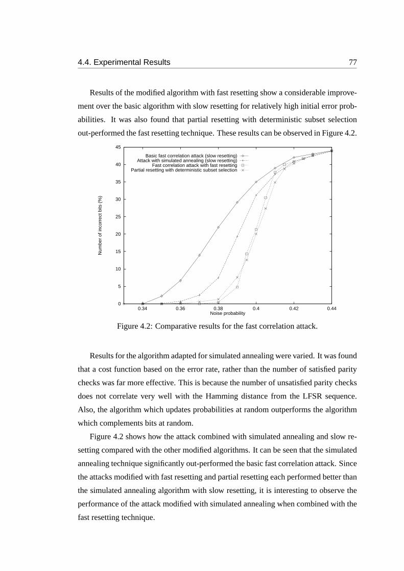
4.4. Experimental Results 77
Results of the modified algorithm with fast resetting show a considerable improve-
ment over the basic algorithm with slow resetting for relatively high initial error prob-
abilities. It was also found that partial resetting with deterministic subset selection
out-performed the fast resetting technique. These results can be observed in Figure 4.2.
0
5
10
15
20
25
30
35
40
45
0.34 0.36 0.38 0.4 0.42 0.44
Num
ber
of in
corr
ect b
its (
%)
Noise probability
Basic fast correlation attack (slow resetting)Attack with simulated annealing (slow resetting)
Fast correlation attack with fast resettingPartial resetting with deterministic subset selection
Figure 4.2: Comparative results for the fast correlation attack.
Results for the algorithm adapted for simulated annealing were varied. It was found
that a cost function based on the error rate, rather than the number of satisfied parity
checks was far more effective. This is because the number of unsatisfied parity checks
does not correlate very well with the Hamming distance from the LFSR sequence.
Also, the algorithm which updates probabilities at random outperforms the algorithm
which complements bits at random.
Figure 4.2 shows how the attack combined with simulated annealing and slow re-
setting compared with the other modified algorithms. It can be seen that the simulated
annealing technique significantly out-performed the basic fast correlation attack. Since
the attacks modified with fast resetting and partial resetting each performed better than
the simulated annealing algorithm with slow resetting, it is interesting to observe the
performance of the attack modified with simulated annealing when combined with the
fast resetting technique.

78 Chapter 4. Attacks on a Certain Class of Stream Ciphers
The results in Figure 4.3 give a comparison of the basic fast correlation attack
with fast resetting and the two algorithms modified with simulated annealing. It can
be seen that for noise probabilities greater than 0.4 the fast correlation attack with
simulated annealing and fast resetting performed slightly better that the fast correlation
attack alone. However for the lower noise probabilities the addition of the simulated
annealing to the attack was less beneficial.
0
5
10
15
20
25
30
35
40
45
0.36 0.38 0.4 0.42 0.44
Num
ber
of in
corr
ect b
its (
%)
Noise probability
Attack with simulated annealing (slow resetting)Attack with simulated annealing (fast resetting)
Basic FCA with fast resetting
Figure 4.3: Comparative results for fast correlation attack modified with simulatedannealing.
Because of the complexity added by the annealing algorithm, combined with the
limited improvement that it gained over the fast resetting technique, the annealing ap-
proach is not considered in the following section which compares the fast resetting
technique with a technique which was proposed by MacKay, namely free energy min-
imisation, which was described above in Section 4.3.
4.4.2 FCA versus FEM
In this section experimental results are presented for the fast correlation attacks based
on the basic fast correlation attack, the attack modified with fast resetting and a free
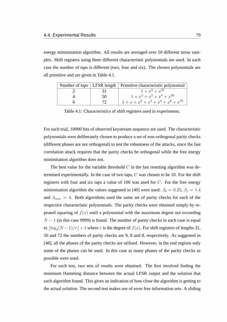
4.4. Experimental Results 79
energy minimisation algorithm. All results are averaged over 50 different noise sam-
ples. Shift registers using three different characteristic polynomials are used. In each
case the number of taps is different (two, four and six). The chosen polynomials are
all primitive and are given in Table 4.1.
Number of taps LFSR length Primitive characteristic polynomial2 31 1 + x3 + x31
4 50 1 + x2 + x3 + x4 + x50
6 72 1 + x + x2 + x3 + x4 + x6 + x72
Table 4.1: Characteristics of shift registers used in experiments.
For each trial, 10000 bits of observed keystream sequence are used. The characteristic
polynomials were deliberately chosen to produce a set of non-orthogonal parity checks
(different phases are not orthogonal) to test the robustness of the attacks, since the fast
correlation attack requires that the parity checks be orthogonal while the free energy
minimisation algorithm does not.
The best value for the variable thresholdC in the fast resetting algorithm was de-
termined experimentally. In the case of two taps,C was chosen to be 10. For the shift
registers with four and six taps a value of 100 was used forC. For the free energy
minimisation algorithm the values suggested in [40] were used:β0 = 0.25, βf = 1.4
andβmax = 4. Both algorithms used the same set of parity checks for each of the
respective characteristic polynomials. The parity checks were obtained simply by re-
peated squaring off(x) until a polynomial with the maximum degree not exceeding
N − 1 (in this case 9999) is found. The number of parity checks in each case is equal
to blog2(N − 1)/rc+1 wherer is the degree off(x). For shift registers of lengths 31,
50 and 72 the numbers of parity checks are 9, 8 and 8, respectively. As suggested in
[48], all the phases of the parity checks are utilised. However, in the end regions only
some of the phases can be used. In this case as many phases of the parity checks as
possible were used.
For each test, two sets of results were obtained. The first involved finding the
minimum Hamming distance between the actual LFSR output and the solution that
each algorithm found. This gives an indication of how close the algorithm is getting to
the actual solution. The second test makes use of error free information sets. A sliding
80 Chapter 4. Attacks on a Certain Class of Stream Ciphers
window technique [53] is used in which a search forr consecutive bits satisfying the
characteristic polynomial is made (r is the shift register length). Ifr such bits can be
found, then the attack is deemed successful.
It is clear from each of Figures 4.4 to 4.6 that the fast resetting algorithm outper-
forms MacKay’s free energy minimisation algorithm for each considered number of
taps. It can also be seen that the free energy minimisation algorithm performs better
than the basic correlation attack algorithm if the number of taps increases. The two
testing techniques, minimum Hamming distance and error free information sets, ap-
pear to correlate well with the results being consistent in all the cases except when the
number of taps is six and the probability is 0.26. Here the Hamming distance result
shows fast resetting to be superior but the result obtained using the information set
technique shows the free energy minimisation algorithm to be (just slightly) better.
According to [55], the critical noise probability beyond which successful iterative
error correction is not possible can be approximated (the exact expression can be found
in [55]) as
pcr =1−M
1w−1w
2(4.13)
whereMw is the average number of parity checks (of weightw + 1) per bit used in the
algorithm. This is of particular interest for the original fast correlation attack with slow
resetting and orthogonal parity checks. In the three cases examined,M2 = 22.248,
M4 = 33.625 andM6 = 43.148, so thatpcr is then given as0.477, 0.345 and0.265,
respectively. These noise probabilities are in accordance with the experimental results
shown in Figures 4.4 to 4.6. So, ifp > pcr, then the fast correlation attacks are bound
to fail on the average. However, it may be possible to extend the set of low weight
parity checks by using techniques other than repeated squaring (see [26]) which in
turn increases the critical noise probability.
4.5 Summary
In this chapter a number of approaches for attacking a certain stream cipher model,
namely the one in Figure 4.1, have been considered. In the introduction an overview
of these ciphers was given, along with a description of the fast correlation attack as
proposed by Meier and Staffelbach [48].
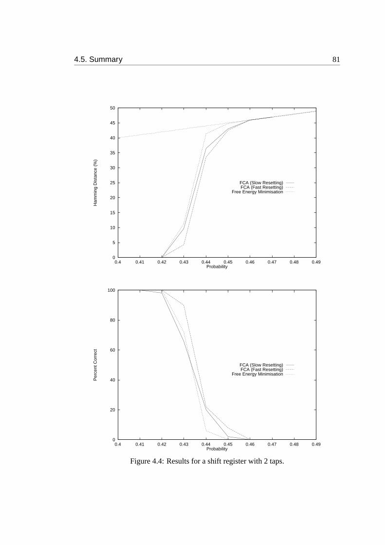
4.5. Summary 81
0
5
10
15
20
25
30
35
40
45
50
0.4 0.41 0.42 0.43 0.44 0.45 0.46 0.47 0.48 0.49
Ham
min
g D
ista
nce
(%)
Probability
FCA (Slow Resetting)FCA (Fast Resetting)
Free Energy Minimisation
0
20
40
60
80
100
0.4 0.41 0.42 0.43 0.44 0.45 0.46 0.47 0.48 0.49
Per
cent
Cor
rect
Probability
FCA (Slow Resetting)FCA (Fast Resetting)
Free Energy Minimisation
Figure 4.4: Results for a shift register with 2 taps.
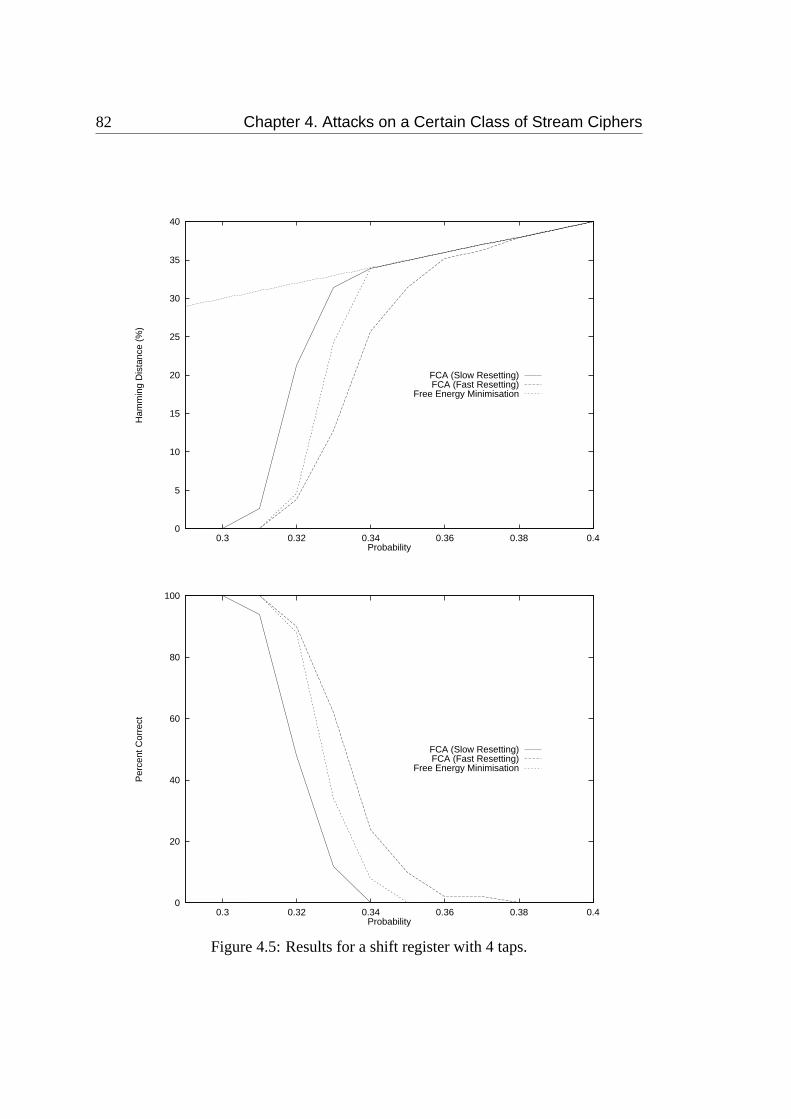
82 Chapter 4. Attacks on a Certain Class of Stream Ciphers
0
5
10
15
20
25
30
35
40
0.3 0.32 0.34 0.36 0.38 0.4
Ham
min
g D
ista
nce
(%)
Probability
FCA (Slow Resetting)FCA (Fast Resetting)
Free Energy Minimisation
0
20
40
60
80
100
0.3 0.32 0.34 0.36 0.38 0.4
Per
cent
Cor
rect
Probability
FCA (Slow Resetting)FCA (Fast Resetting)
Free Energy Minimisation
Figure 4.5: Results for a shift register with 4 taps.
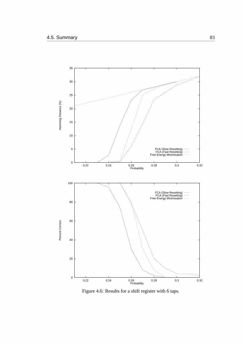
4.5. Summary 83
0
5
10
15
20
25
30
35
0.22 0.24 0.26 0.28 0.3 0.32
Ham
min
g D
ista
nce
(%)
Probability
FCA (Slow Resetting)FCA (Fast Resetting)
Free Energy Minimisation
0
20
40
60
80
100
0.22 0.24 0.26 0.28 0.3 0.32
Per
cent
Cor
rect
Probability
FCA (Slow Resetting)FCA (Fast Resetting)
Free Energy Minimisation
Figure 4.6: Results for a shift register with 6 taps.
84 Chapter 4. Attacks on a Certain Class of Stream Ciphers
Several modifications were suggested which allows the fast correlation attack to
recover initial LFSR contents for ciphers with a higher noise probability than the origi-
nal search allowed. This has been shown in the experimental results. The fast resetting
technique provides significant improvement by preventing the algorithm from arriving
at a locally minimum solution. Similarly, by updating a subset of the probability vec-
tor in any iteration, using either deterministic techniques or a random selection, it was
found that higher noise probabilities could be compromised.
In a further experiment, simulated annealing was used in combination with the fast
correlation attack in an attempt to attack even greater noise probabilities. While this
technique provided a significant improvement of the basic algorithm as published by
Meier and Staffelbach, it was found to not significantly improve the other modifica-
tions outlined - that is, fast resetting alone and deterministic and random probability
updates.
Chapter 5
The Knapsack Cipher: What Not ToDo
The success of the approximate algorithms which were presented in Chapter 2 is de-
pendent upon the availability of a suitable solution evaluation mechanism. Such a
mechanism (a fitness function or a cost function) must accurately assess every feasible
solution giving an indication of its optimality - i.e., how close it is to the optimal solu-
tion. In this chapter an example of a problem for which no suitable solution assessment
exists is presented. The problem in question is theknapsackproblem. Spillman [71]
presented a genetic algorithm which he claimed could solve large instances of the
knapsack problem. This chapter shows that such an approach has little merit, due to
the lack of a suitable fitness function.
A description of the Merkle-Hellman cryptosystem is given in Appendix C. The
processes of encryption and decryption are outlined, along with the method used to
generate the public/private key pair. The Merkle-Hellman cryptosystem was shown to
be insecure in the early 1980’s by Shamir [68]. Details of Shamir’s attack which is
based upon the structure of the secret key is given in Appendix C.
The attack proposed by Spillman uses an entirely different approach. Rather than
attacking the structure of the secret key, Spillman’s approach was to determine the
original message by finding the elements of the public key which were added together
to obtain the ciphertext. In Section 5.1 the fitness function which was suggested by
Spillman [73] is analysed and an alternative proposed. It will be shown that there is no
truly suitable fitness function for attacks on the knapsack cipher using the technique
discussed in this chapter. Section 5.2 presents an algorithm similar to the one proposed
85
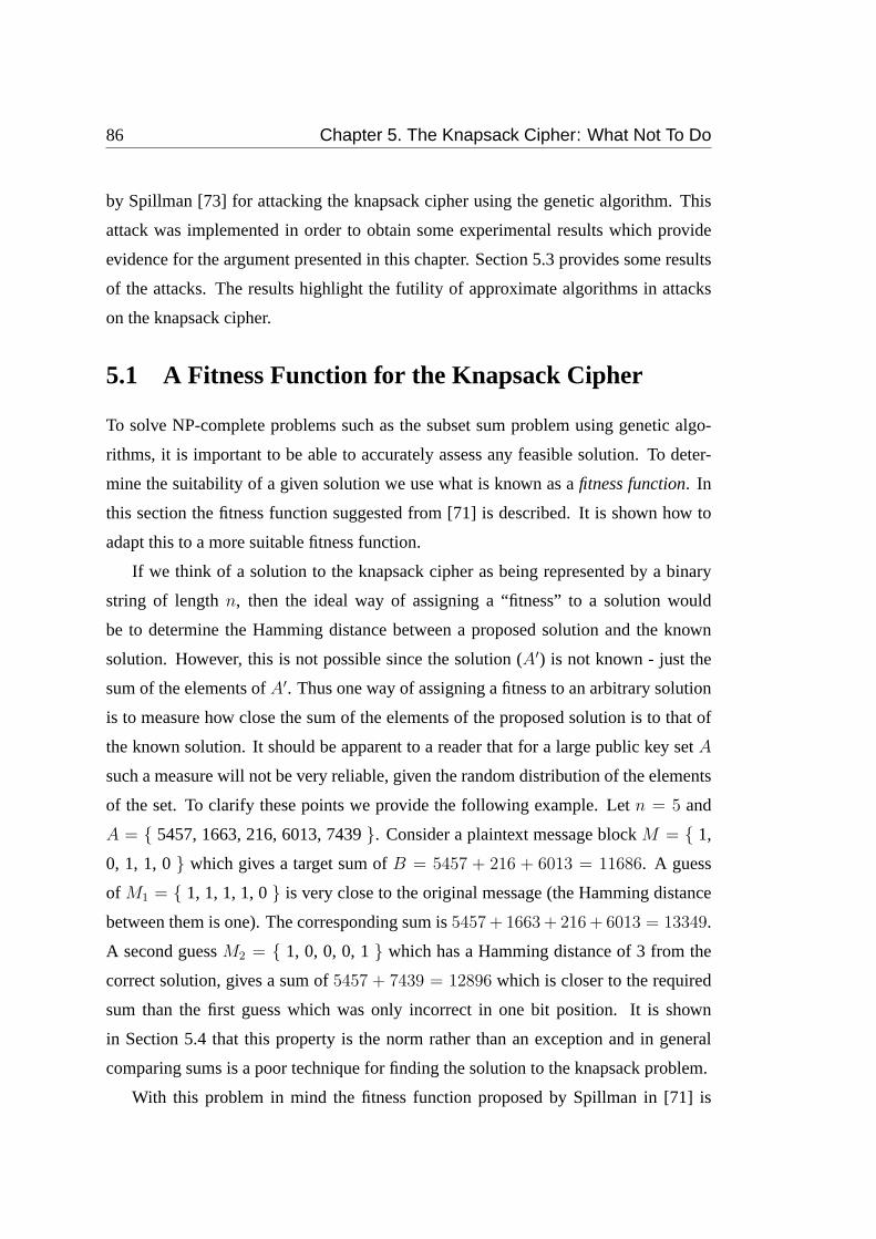
86 Chapter 5. The Knapsack Cipher: What Not To Do
by Spillman [73] for attacking the knapsack cipher using the genetic algorithm. This
attack was implemented in order to obtain some experimental results which provide
evidence for the argument presented in this chapter. Section 5.3 provides some results
of the attacks. The results highlight the futility of approximate algorithms in attacks
on the knapsack cipher.
5.1 A Fitness Function for the Knapsack Cipher
To solve NP-complete problems such as the subset sum problem using genetic algo-
rithms, it is important to be able to accurately assess any feasible solution. To deter-
mine the suitability of a given solution we use what is known as afitness function. In
this section the fitness function suggested from [71] is described. It is shown how to
adapt this to a more suitable fitness function.
If we think of a solution to the knapsack cipher as being represented by a binary
string of lengthn, then the ideal way of assigning a “fitness” to a solution would
be to determine the Hamming distance between a proposed solution and the known
solution. However, this is not possible since the solution (A′) is not known - just the
sum of the elements ofA′. Thus one way of assigning a fitness to an arbitrary solution
is to measure how close the sum of the elements of the proposed solution is to that of
the known solution. It should be apparent to a reader that for a large public key setA
such a measure will not be very reliable, given the random distribution of the elements
of the set. To clarify these points we provide the following example. Letn = 5 and
A = { 5457, 1663, 216, 6013, 7439}. Consider a plaintext message blockM = { 1,
0, 1, 1, 0} which gives a target sum ofB = 5457 + 216 + 6013 = 11686. A guess
of M1 = { 1, 1, 1, 1, 0} is very close to the original message (the Hamming distance
between them is one). The corresponding sum is5457 + 1663 + 216 + 6013 = 13349.
A second guessM2 = { 1, 0, 0, 0, 1} which has a Hamming distance of 3 from the
correct solution, gives a sum of5457 + 7439 = 12896 which is closer to the required
sum than the first guess which was only incorrect in one bit position. It is shown
in Section 5.4 that this property is the norm rather than an exception and in general
comparing sums is a poor technique for finding the solution to the knapsack problem.
With this problem in mind the fitness function proposed by Spillman in [71] is
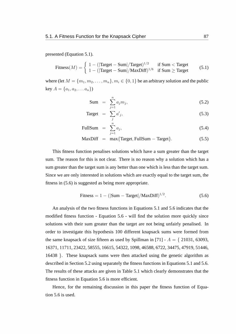
5.1. A Fitness Function for the Knapsack Cipher 87
presented (Equation 5.1).
Fitness(M) =
{1− (|Target− Sum|/Target)1/2 if Sum< Target1− (|Target− Sum|/MaxDiff)1/6 if Sum≥ Target
(5.1)
where (letM = {m1,m2, . . . , mn},mi ∈ {0, 1} be an arbitrary solution and the public
keyA = {a1, a2, . . . an})
Sum =n∑
j=1
ajmj, (5.2)
Target =∑
j
a′j, (5.3)
FullSum =n∑
j=1
aj, (5.4)
MaxDiff = max{Target, FullSum− Target}. (5.5)
This fitness function penalises solutions which have a sum greater than the target
sum. The reason for this is not clear. There is no reason why a solution which has a
sum greater than the target sum is any better than one which is less than the target sum.
Since we are only interested in solutions which are exactly equal to the target sum, the
fitness in (5.6) is suggested as being more appropriate.
Fitness= 1− (|Sum− Target|/MaxDiff)1/2. (5.6)
An analysis of the two fitness functions in Equations 5.1 and 5.6 indicates that the
modified fitness function - Equation 5.6 - will find the solution more quickly since
solutions with their sum greater than the target are not being unfairly penalised. In
order to investigate this hypothesis 100 different knapsack sums were formed from
the same knapsack of size fifteen as used by Spillman in [71] -A = { 21031, 63093,
16371, 11711, 23422, 58555, 16615, 54322, 1098, 46588, 6722, 34475, 47919, 51446,
16438}. These knapsack sums were then attacked using the genetic algorithm as
described in Section 5.2 using separately the fitness functions in Equations 5.1 and 5.6.
The results of these attacks are given in Table 5.1 which clearly demonstrates that the
fitness function in Equation 5.6 is more efficient.
Hence, for the remaining discussion in this paper the fitness function of Equa-
tion 5.6 is used.
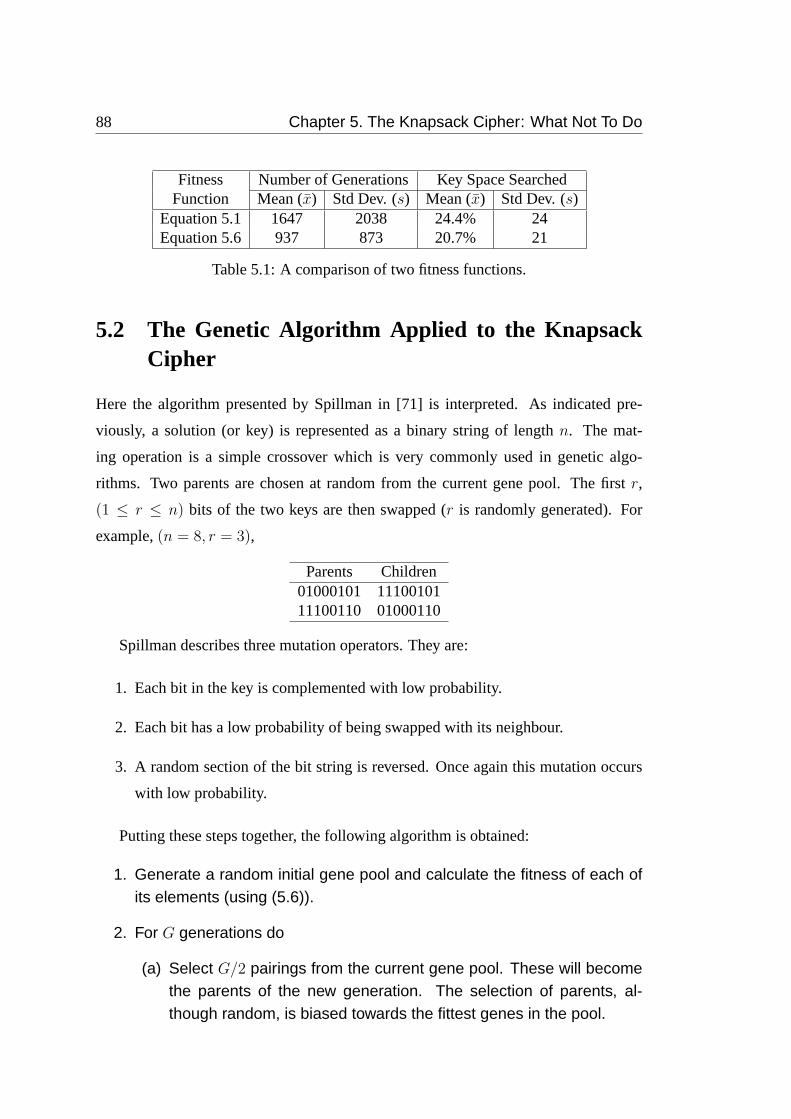
88 Chapter 5. The Knapsack Cipher: What Not To Do
Fitness Number of Generations Key Space SearchedFunction Mean (x) Std Dev. (s) Mean (x) Std Dev. (s)
Equation 5.1 1647 2038 24.4% 24Equation 5.6 937 873 20.7% 21
Table 5.1: A comparison of two fitness functions.
5.2 The Genetic Algorithm Applied to the KnapsackCipher
Here the algorithm presented by Spillman in [71] is interpreted. As indicated pre-
viously, a solution (or key) is represented as a binary string of lengthn. The mat-
ing operation is a simple crossover which is very commonly used in genetic algo-
rithms. Two parents are chosen at random from the current gene pool. The firstr,
(1 ≤ r ≤ n) bits of the two keys are then swapped (r is randomly generated). For
example,(n = 8, r = 3),
Parents Children01000101 1110010111100110 01000110
Spillman describes three mutation operators. They are:
1. Each bit in the key is complemented with low probability.
2. Each bit has a low probability of being swapped with its neighbour.
3. A random section of the bit string is reversed. Once again this mutation occurs
with low probability.
Putting these steps together, the following algorithm is obtained:
1. Generate a random initial gene pool and calculate the fitness of each ofits elements (using (5.6)).
2. For G generations do
(a) Select G/2 pairings from the current gene pool. These will becomethe parents of the new generation. The selection of parents, al-though random, is biased towards the fittest genes in the pool.
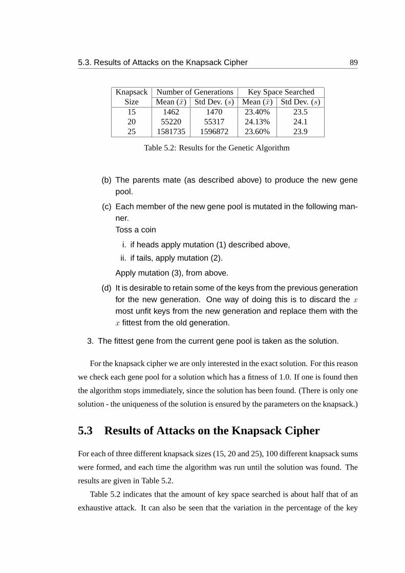
5.3. Results of Attacks on the Knapsack Cipher 89
Knapsack Number of Generations Key Space SearchedSize Mean (x) Std Dev. (s) Mean (x) Std Dev. (s)15 1462 1470 23.40% 23.520 55220 55317 24.13% 24.125 1581735 1596872 23.60% 23.9
Table 5.2: Results for the Genetic Algorithm
(b) The parents mate (as described above) to produce the new genepool.
(c) Each member of the new gene pool is mutated in the following man-ner.Toss a coin
i. if heads apply mutation (1) described above,
ii. if tails, apply mutation (2).
Apply mutation (3), from above.
(d) It is desirable to retain some of the keys from the previous generationfor the new generation. One way of doing this is to discard the x
most unfit keys from the new generation and replace them with thex fittest from the old generation.
3. The fittest gene from the current gene pool is taken as the solution.
For the knapsack cipher we are only interested in the exact solution. For this reason
we check each gene pool for a solution which has a fitness of 1.0. If one is found then
the algorithm stops immediately, since the solution has been found. (There is only one
solution - the uniqueness of the solution is ensured by the parameters on the knapsack.)
5.3 Results of Attacks on the Knapsack Cipher
For each of three different knapsack sizes (15, 20 and 25), 100 different knapsack sums
were formed, and each time the algorithm was run until the solution was found. The
results are given in Table 5.2.
Table 5.2 indicates that the amount of key space searched is about half that of an
exhaustive attack. It can also be seen that the variation in the percentage of the key
90 Chapter 5. The Knapsack Cipher: What Not To Do
space searched, as well as the number of generations required by the algorithm, is
large.
It is worth noting that although the methods discussed in this chapter do provide
some improvement over an exhaustive search in terms of the amount of key space
searched (on the average an exhaustive search would traverse 50% of the key space be-
fore finding the correct solution), in practice an exhaustive search will complete more
quickly than a genetic algorithm search due to the large decrease in the complexity. It
is very quick to test an arbitrary solution without determining its fitness, mutating it
and combining it with other solutions - as happens in the genetic algorithm. This point
further highlights the unsuitability of combinatorial optimisation in solving the subset
sum problem in this manner.
5.4 Correlation Between Hamming Distance and Fit-ness
The reason for this attack being poor lies with the fact that the fitness function does
not accurately describe the suitability of a given solution. This is because the fitness
function does not always give a true indication of the Hamming distance between the
proposed solution and the solution sought. To show this we investigate the distribution
of Hamming distances for particular regions of fitness values. We are particularly
interested in possible solutions which have a high fitness value. The results (shown in
Table 5.3) were obtained using a randomly generated knapsack of size 30. The fitness
of all possible (i.e.230) solutions was calculated, along with the Hamming distance
of each solution from the desired solution. Table 5.3 clearly shows that a high fitness
value does not necessarily mean a low Hamming distance. In fact the distribution of
Hamming distances for a given range of fitness values appears to be ‘binomial’-like. It
can also be seen from Table 5.3 that the fitness values very close to 1.0 the distribution
remains very spread. That is, there are solutions with a very high fitness value which
have Hamming distances that are by no means close to that of the required solution.
In a recent paper by Spillman [72] addressing the use of genetic algorithms in
solving the knapsack problem it was suggested that a “local search” routine would
speed up the search. This routine involved taking solutions with a high fitness (greater
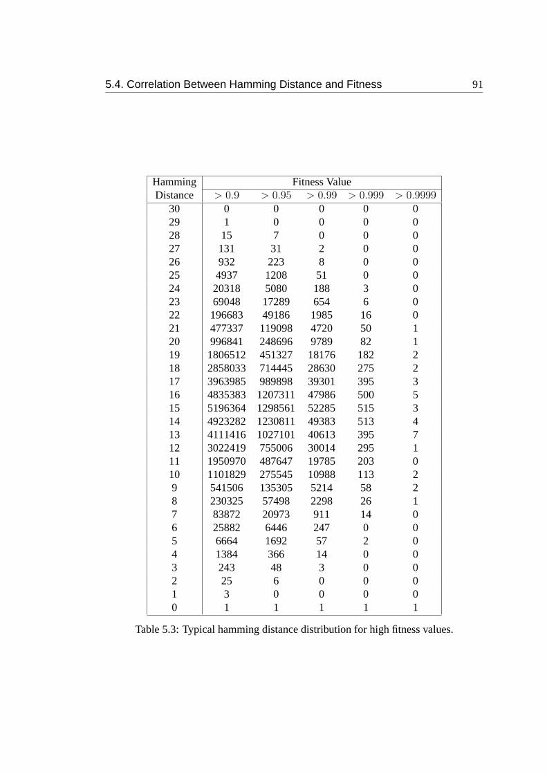
5.4. Correlation Between Hamming Distance and Fitness 91
Hamming Fitness ValueDistance > 0.9 > 0.95 > 0.99 > 0.999 > 0.9999
30 0 0 0 0 029 1 0 0 0 028 15 7 0 0 027 131 31 2 0 026 932 223 8 0 025 4937 1208 51 0 024 20318 5080 188 3 023 69048 17289 654 6 022 196683 49186 1985 16 021 477337 119098 4720 50 120 996841 248696 9789 82 119 1806512 451327 18176 182 218 2858033 714445 28630 275 217 3963985 989898 39301 395 316 4835383 1207311 47986 500 515 5196364 1298561 52285 515 314 4923282 1230811 49383 513 413 4111416 1027101 40613 395 712 3022419 755006 30014 295 111 1950970 487647 19785 203 010 1101829 275545 10988 113 29 541506 135305 5214 58 28 230325 57498 2298 26 17 83872 20973 911 14 06 25882 6446 247 0 05 6664 1692 57 2 04 1384 366 14 0 03 243 48 3 0 02 25 6 0 0 01 3 0 0 0 00 1 1 1 1 1
Table 5.3: Typical hamming distance distribution for high fitness values.
92 Chapter 5. The Knapsack Cipher: What Not To Do
than 0.95) and complementing each bit of the solution, one by one. If the fitness
improved then the adjusted solution was accepted. Table 5.3 indicates that such a
routine will have very little affect on the efficiency of the algorithm since the fitness
equation is not representative of the Hamming distance. In fact for the example in Table
5.3 this method would never have found the optimum since there were no solutions
with a fitness greater than 0.95 and a Hamming distance of 1 from the solution sought.
5.5 Summary
The purpose of this chapter was to highlight the fact that combinatorial optimisation
techniques rely heavily upon the suitability of the solution evaluation technique (fitness
or cost). It has been shown, that for the subset sum problem, there is no (known)
suitable evaluation technique when solving based on the subset sum. This is why
the Merkle-Hellman cryptosystem is so elegant - a known NP-complete problem has
been converted to an NP-hard problem and utilised as a cryptosystem. Of course the
weakness with the cryptosystem is in the structure of the secret key rather than the
actual encryption process (which Spillman has attempted to attack).
Spillman’s fitness is based on the difference between the sum of a proposed solution
and the known target sum. As Table 5.3 shows, such an approach gives no indication
of the Hamming distance between the proposed solution and the binary representation
of the target solution which is sought. Thus basing an genetic algorithm upon such a
fitness function is inappropriate. This is further illustrated by the results in Table 5.2
which indicate that approximately one quarter of the solution space is searched, on
the average, before the correct solution is found. This is not significantly better than
an exhaustive search and, in fact, when complexity is considered, is worse due to the
simplicity of an exhaustive search compared to the genetic algorithm search.
Chapter 6
Finding Cryptographically SoundBoolean Functions
The previous three chapters of this thesis have looked at the use of optimisation heuris-
tics in the field ofcryptanalysis. In this chapter a useful application of the genetic
algorithm to the field ofcryptographyis presented. The genetic algorithm is used to
search for cryptographically sound Boolean functions. Most block and stream ciphers
incorporate Boolean functions which are chosen, in general, to satisfy a number of
cryptographic criteria. Because many cryptographic properties of Boolean functions
conflict with each other, the final choice of functions is usually a compromise between
the desired properties of the functions.
An introduction to the theory and cryptographic properties of Boolean functions
is given in Appendix D. In this chapter the property of nonlinearity is considered,
although the work could be extended to include other cryptographic properties. When
designing cryptosystems (ciphers) careful consideration must be given to the choice of
functions used. High nonlinearity is an extremely important property required in order
to reduce the effectiveness of attacks such as linear cryptanalysis – recently proposed
by Matsui [45].
In this chapter a number of algorithms are introduced which assist with finding
Boolean functions with good cryptographic properties. A new approach is used to
determining bit positions in a function’s truth table which, when complemented, will
improve the nonlinearity of the function. The theory behind this principle, which is
based on the coefficients of the Walsh-Hadamard transform (WHT – see Appendix D),
is described in Section 6.1. It is also shown in this section that the balance of the
93
94 Chapter 6. Finding Cryptographically Sound Boolean Functions
function can either be improved or maintained as required.
A basic hill climbing technique which makes use of this new approach is described
in Section 6.2. This technique is modified to incorporate a genetic algorithm in Sec-
tion 6.3. It is shown that these new search techniques are extremely powerful when
compared to traditional random search techniques. Experimental results reinforcing
the techniques’ usefulness are given in Section 6.4. These techniques represent novel
methods of systematically generating highly nonlinear Boolean functions.
6.1 Improving Nonlinearity
Consider altering a Boolean function by complementing its binary truth table in a sin-
gle position such that the nonlinearity is improved. Each truth table position corre-
sponds to a unique function input. A technique is now introduced which enables the
creation of a complete list of Boolean function inputs such that complementing any one
of the corresponding truth table positions will increase the nonlinearity of the function.
This list of truth table positions is referred to as the 1-Improvement Set off(x), or 1-
ISf for short. A formal definition of the 1-ISf is now given.
Definition 1 Let g(x) = f(x) ⊕ 1 for x = xa and g(x) = f(x) for all other x. If
Ng > Nf thenxa ∈ 1-ISf .
Of course the set may be empty in which casef(x) is referred to as 1-locally max-
imum for nonlinearity and cannot be improved using the technique described below.
Since all Bent functions (see Appendix D) are globally maximum, their 1-Improvement
Sets must be empty. There also exist sub-optimum local maxima that will be found by
hill climbing algorithms. It is computationally intensive to exhaustively alter truth ta-
ble positions, find new WHTs and determine the set 1-ISf . Thus, a fast, systematic
method of determining the 1-Improvement Set of a given Boolean function from its
truth table and Walsh-Hadamard transform is sought. In this section a set of conditions
are presented which provide a method of determining whether or not an inputx is in
the 1-Improvement Set.
In order to find the 1-ISf of a Boolean function it is first necessary to find values
of the Walsh-Hadamard transform coefficients which correspond to values close in
absolute value to the maximum coefficient value, WHMAX .
6.1. Improving Nonlinearity 95
Definition 2 Let f(x) be a Boolean function with Walsh-Hadamard transformF (ω)
where WHMAX denotes the maximum absolute value ofF (ω). There will exist one or
more linear functionsLω(x) that have minimum distance tof(x), and|F (ω)| = WHMAX
for theseω. The following sets are defined:
W+1 = {ω : F (ω) = WHMAX} and
W−1 = {ω : F (ω) = −WHMAX}.
Also needed are the sets ofω for which the WHT magnitude is close to the maximum:
W+2 = {ω : F (ω) = WHMAX− 2},
W−2 = {ω : F (ω) = −(WHMAX− 2)},
W+3 = {ω : F (ω) = WHMAX− 4}, and
W−3 = {ω : F (ω) = −(WHMAX− 4)}.
When a truth table is changed in exactly one place, all WHT values are changed by
+2 or -2. It follows that in order to increase the nonlinearity the WHT values in setW+1
must change by -2, the WHT values in setW−1 must change by +2, and also the WHT
values in setW+2 must change by -2 and the WHT values in setW−
2 must change by
+2. The first two conditions are obvious, and the second two conditions are required
so that all other|F (ω)| remain less than WHMAX . These conditions can be translated
into simple tests.
Theorem 1 Given a Boolean functionf(x) with WHTF (ω), define setsW+ = W+1 ∪
W+2 andW− = W−
1 ∪W−2 . For an inputx to be an element of the Improvement Set,
the following two conditions must be satisfied.
(i) f(x) = Lω(x) for all ω ∈ W+, and
(ii) f(x) 6= Lω(x) for all ω ∈ W−.
If the functionf(x) is not balanced, a reduction in the imbalance can be achieved by
imposing the additional restriction that
(iii) when F (0) > 0, f(x) = 0, elsef(x) = 1.
96 Chapter 6. Finding Cryptographically Sound Boolean Functions
Proof: Start by considering the conditions to make WHT values change by a desired
amount. WhenF (ω) is positive, there are more 1 than -1 in the polarity truth table,
and more 0 than 1 in the binary truth table off(x) ⊕ Lω(x). Thus changing a single
0, in the truth table off(x) ⊕ Lω(x), to a 1 will make∆F (ω) = −2. This means
that an input,x, is selected such thatf(x) = Lω(x). A change of -2 is desired for all
WHT values withω ∈ W+, so this proves condition (i). A similar argument proves
condition (ii). A function is balanced whenF (0) = 0, so to reduce the imbalancex
must be selected according to condition (iii). 2
To further clarify the task of determining the 1-Improvement Set of a given Boolean
function,f(x), consider the following example.
Example 6.1 Consider the function described by the truth table given in Table 6.1.
The corresponding Walsh-Hadamard transform is also given. Observe that WHMAX = 8
is attained forω = 0101 and ω = 1110. There are no transform values equal to
WHMAX − 2 = 6, soW+1 = {0101, 1110} andW−
1 = W+2 = W−
2 = φ. Thus, from
Theorem 1, candidate values for the 1-ISf occur whenL0101(x) = L1110(x) = f(x).
Thus 1-ISf = {0000, 0011, 0100, 0111, 1001, 1010, 1101, 1110} and complementing
any one of the corresponding truth table bits (thef(x) column) will increase the non-
linearity fromNf = 12(2n −WHMAX) = 4 to Nf = 5.
It is often desirable to improve the nonlinearity of balanced Boolean functions,
while retaining balance. Clearly this requires an even number of truth table changes.
A set of conditions are now presented which define a pair of inputsxa, xb so that
complementing both their function values causes an increase in nonlinearity, without
changing the Hamming weight. The 2-Improvement Set, 2-ISf , is defined as the set of
all such input pairs. A function for which no pair satisfies these conditions is said to
be 2-locally maximum.
Theorem 2 Given a Boolean functionf(x) with WHTF (ω), define setsW1 = W+1 ∪
W−1 , W+
2,3 = W+2 ∪ W+
3 andW−2,3 = W−
2 ∪ W−3 . A pair of inputs(xa, xb) is in the
2-Improvement Set off(x) if and only if all of the following conditions are satisfied:
(i) f(xa) 6= f(xb),
(ii) Lω(xa) 6= Lω(xb) for all ω ∈ W1,

6.1. Improving Nonlinearity 97
x/ω f(x) F (ω) L0101(x) L1110(x) x ∈ 1-ISf?0000 0 0 0 0
√0001 1 4 1 00010 0 0 0 10011 1 4 1 1
√0100 1 4 1 1
√0101 1 8 0 10110 1 -4 1 00111 0 0 0 0
√1000 0 -4 0 11001 1 0 1 1
√1010 0 -4 0 0
√1011 0 0 1 01100 0 0 1 01101 0 4 0 0
√1110 1 8 1 1
√1111 1 -4 0 1
Table 6.1: Table for Example 6.1.
(iii) f(xi) = Lω(xi), i ∈ {1, 2}, for all ω ∈ W+1 ,
(iv) f(xi) 6= Lω(xi), i ∈ {1, 2}, for all ω ∈ W−1 ,
(v) for all ω ∈ W+2,3, if Lω(xa) 6= Lω(xb) thenf(xi) = Lω(xi), i ∈ {1, 2}, and
(vi) for all ω ∈ W−2,3, if Lω(xa) 6= Lω(xb) thenf(xi) 6= Lω(xi), i ∈ {1, 2}.
Proof: Condition (i) is required to maintain the Hamming weight. Conditions (iii) and
(iv) are proven similarly to Theorem 1 (condition (ii) follows from (iii) and (iv)). In
order to stop the correlation to other linear functions increasing too much, it is required
that∆F (ω) 6= +4, for all ω ∈ W+2,3, and it follows that not both off(xi)⊕Lω(xi) = 1,
or equivalently that at least one off(xi)⊕ Lω(xi) = 0. Consequently,
[f(xa)⊕ Lω(xa)][f(xb)⊕ Lω(xb)] = 0,
and expanding this, noting from (i) thatf(xa)f(xb) = 0, it follows that
f(xa)Lω(xb)⊕ f(xb)Lω(xa)⊕ Lω(xa)Lω(xb) = 0.
Four cases need to be considered in order to find the exact conditions under which this
expression will be satisfied:
98 Chapter 6. Finding Cryptographically Sound Boolean Functions
(a) WhenLω(xa) = Lω(xb) = 0 the expression is satisfied and no further conditions
on (xa, xb) are required.
(b) WhenLω(xa) = Lω(xb) = 1 the expression becomesf(xa)⊕ f(xb) = 1 which
is equivalent to condition (i).
(c) WhenLω(xa) = 0 andLω(xb) = 1 the expression becomesf(xa) = 0.
(d) WhenLω(xa) = 1 andLω(xb) = 0 the expression becomesf(xb) = 0.
Combining (a)-(d) it can be seen that whenLω(xa) 6= Lω(xb) for ω ∈ W+2,3 it is
required thatf(xi) = Lω(xi), i = 1, 2, thus proving condition (v). The Proof of (vi) is
similar. 2
The following theorem shows how to modify the WHT of a Boolean function that
has been altered in a single truth table position, with complexityO(2n). It is noted that
the algorithm for incremental improvement of Boolean functions suggested in [17]
recomputes the WHT after every single bit change regardless of whether that change
improves the nonlinearity. Therefore the algorithms presented here are superior on two
counts - every change is an improvement and the new WHT is foundn times faster.
Theorem 3 Let g(x) be obtained fromf(x) by complementing the output for a single
input, xa. Then each component of the WHT ofg(x), G(ω) = F (ω) + ∆(ω), can be
obtained as follows: Iff(xa) = Lω(xa), then∆(ω) = −2, else∆(ω) = +2.
Proof: Whenf(xa) = Lω(x), it follows that(−1)f(xa)⊕Lω(xa) = 1, which contributes
to the sum inF (xa). Changing the value off(xa) changes this contribution to -1, so
∆F (ω) = −2. Similarly whenf(xa) 6= Lω(x), ∆F (ω) = +2. 2
This idea is further clarified by continuing Example 6.1 so that a particular posi-
tion is complemented and the new Walsh-Hadamard transform calculated. Consider
Example 6.2.
Example 6.2 Consider the functionf(x) which was presented in Example 6.1. It was
shown that the 1-ISf = {0000, 0011, 0100, 0111, 1001, 1010, 1101, 1110}. Suppose
the truth table bit corresponding to inputxa = 0100 is complemented to give a new
functiong(x). Theorem 3 states that the change in the Walsh-Hadamard transform
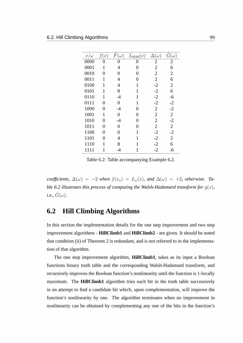
6.2. Hill Climbing Algorithms 99
x/ω f(x) F (ω) L0100(x) ∆(ω) G(ω)0000 0 0 0 2 20001 1 4 0 2 60010 0 0 0 2 20011 1 4 0 2 60100 1 4 1 -2 20101 1 8 1 -2 60110 1 -4 1 -2 -60111 0 0 1 -2 -21000 0 -4 0 2 -21001 1 0 0 2 21010 0 -4 0 2 -21011 0 0 0 2 21100 0 0 1 -2 -21101 0 4 1 -2 21110 1 8 1 -2 61111 1 -4 1 -2 -6
Table 6.2: Table accompanying Example 6.2.
coefficients,∆(ω) = −2 whenf(xa) = Lω(x), and ∆(ω) = +2, otherwise. Ta-
ble 6.2 illustrates this process of computing the Walsh-Hadamard transform forg(x),
i.e.,G(ω).
6.2 Hill Climbing Algorithms
In this section the implementation details for the one step improvement and two step
improvement algorithms -HillClimb1 andHillClimb2 - are given. It should be noted
that condition (ii) of Theorem 2 is redundant, and is not referred to in the implementa-
tion of that algorithm.
The one step improvement algorithm,HillClimb1 , takes as its input a Boolean
functions binary truth table and the corresponding Walsh-Hadamard transform, and
recursively improves the Boolean function’s nonlinearity until the function is 1-locally
maximum. TheHillClimb1 algorithm tries each bit in the truth table successively
in an attempt to find a candidate bit which, upon complementation, will improve the
function’s nonlinearity by one. The algorithm terminates when no improvement in
nonlinearity can be obtained by complementing any one of the bits in the function’s

100 Chapter 6. Finding Cryptographically Sound Boolean Functions
truth table.
• HillClimb1(BF, WHT)
1. Determine the maximum value of the Walsh-Hadamard transform - WHMAX .
2. By parsing the WHT find the values ofω which correspond to transform
values equal to|WHMAX | and |WHMAX − 2|. In this manner create the two
sets:W+ = W+1 ∪W+
2 andW− = W−1 ∪W−
2 .
3. Fori = 1, . . . , 2n, do
(a) Complement theith bit in the truth table ofBF to produce the new
Boolean functionBF′.
(b) By parsing the setsW+ andW− check that conditions (iii) and (iv) of
Theorem 2 above are satisfied forBF. If they are, calculate the updated
Walsh-Hadamard transform -WHT ′ - using Theorem 3 above, and
restart the algorithm - i.e., callHillClimb1(BF ′, WHT ′).
4. BF represents a 1-locally maximum Boolean function - terminate process-
ing.
The second algorithm described here -HillClimb2 - is an implementation of
the steps required to find a 2-locally maximum Boolean function, given a ran-
dom Boolean function as a starting point. The algorithm maintains the balance
of the original function whilst improving the nonlinearity each time two candi-
date bits can be found for complementation. This algorithm must generate two
candidate lists of possible bit positions in the truth table for complementation.
These two lists - calledC0 andC1 - contain candidate positions in the truth ta-
ble with corresponding values of zero and one, respectively. When one position
from each of the setsC0 andC1 is found which satisfy the required conditions
of Theorem 2, the corresponding bits are complemented. The new function’s
Walsh-Hadamard transform is computed efficiently by two successive calls to
the operation described in Theorem 3. The function calls itself in a recursive
manner in an attempt to further improve the new function.
• HillClimb2(BF, WHT)

6.3. Using a Genetic Algorithm to Improve the Search 101
1. Determine the maximum value of the WHT - WHMAX .
2. By parsing the WHT obtain the values ofω which correspond to transform
values of|WHMAX |, |WHMAX − 2| and|WHMAX − 4| and hence create the sets
W+1 , W−
1 , W+2,3 = W+
2 ∪W+3 andW−
2,3 = W−2 ∪W−
3 .
3. Fori = 1, . . . , 2n, do
(a) By parsing the setsW+1 andW−
1 ensure that conditions (iii) and (iv) in
Theorem 2 are satisfied forBF. If they are, depending on the value of
theith bit in the truth table, addi to C0 or C1.
4. For each element ofC0, do
(a) For each element ofC1, do
i. Check conditions (v) and (vi) of Theorem 2. If they are satisfied
for BF, complement the corresponding bits in the truth table ofBF
- call the resulting Boolean functionBF′, find the adjusted Walsh-
Hadamard transform -WHT ′ by applying Theorem 3 twice and
call HillClimb2(BF ′, WHT ′).
5. BF represents a 2-locally maximum Boolean function - terminate process-
ing.
6.3 Using a Genetic Algorithm to Improve the Search
The genetic algorithm was described in detail in Chapter 2 and has been used exten-
sively in various cryptanalytic algorithms in the previous chapters. In this chapter the
genetic algorithm is used to improve the hill climbing algorithms described above. In
the classical genetic algorithm the solution is represented as a binary string. The same
representation is utilised here for the Boolean function - in this case the binary string
represents the binary truth table of the function. Given a solution representation, there
are three other requirements of the genetic algorithm, namely a solution evaluation
technique, a mating function and a mutation function. The mating function allows the
combining of solutions, hopefully, in a meaningful manner. Mutation is performed on
a single solution in order to introduce a degree of randomness to the solution pool.
These three genetic algorithm requirements are now discussed individually.
102 Chapter 6. Finding Cryptographically Sound Boolean Functions
The genetic algorithm requires a method of assessing and comparing solutions.
Typically this measure is referred to as the “fitness”. The fitness which is used here
is simply the nonlinearity (Nf ) of the Boolean functionf(x). This is suitable for a
genetic algorithm, since|Nf − Ng| ≤ dist(f(x), g(x)). In other words nonlinearity
is a locally smooth fitness function. With Boolean functions there are also numerous
other fitness functions possible (for example, the maximum value taken by the auto-
correlation function could be minimised).
The genetic algorithm also requires a method for combining two (possibly more)
solutions in order to obtain offspring. The usual mating process utilised in classical
genetic algorithm is often referred to as “crossover”. The crossover operation involves
selecting two “parents” from the current solution pool, picking a random point in the
binary string representing each of the parents and swapping the values beyond that
point between the two parents. This process results in two “children” with some char-
acteristics of each of the parents. Here a slightly different breeding process is used,
namely “merging”, which is described below. Notice that this mating operation is dif-
ferent from ones in previous chapters by the fact that only a single child function is
produced.
Definition 3 Given the binary truth tables of two Boolean functionsf1(x), f2(x) of n
variables at Hamming distanced, the merge operation is defined as:
• If d ≤ 2n−1
MERGEf1,f2(x) =
{f1(x) if f1(x) = f2(x)a random bit, otherwise.
• else
MERGEf1,f2(x) =
{f1(x) if f1(x) 6= f2(x)a random bit, otherwise.
Note that this merging operation is partly deterministic and partly probabilistic, and
that it takes the fact that complementation does not change nonlinearity into account.
The number of distinct children that can result from a merge is given by2dist(f1,f2),
and all are equally probable. Thus the use of MERGE as a breeding scheme includes
implicit mutation. Since random mutation of a highly nonlinear function is likely to re-
duce the nonlinearity, additional random mutations are avoided and instead the merge
6.3. Using a Genetic Algorithm to Improve the Search 103
is relied upon to direct the pool into new areas of the search space. The motivation for
this operation is that two functions that are highly nonlinear and close to each other
will be close to some local maximum, and the merging operation produces a function
also in the same region, hopefully close to that maximum. Also when applied to un-
correlated functions, the merge operation produces children spread over a large area,
thus allowing the genetic algorithm to search the space more fully. At the start of the
genetic algorithm, the children are scattered widely, then as the pool begins to consist
of good functions, the merging assists convergence to local maxima. The experiments
have shown that other simple combining methods, such as XOR and crossover, do not
assist convergence to good solutions. It is the use of merging that allows the genetic
algorithm to be effective.
The mutation operation simply introduces randomness to the solution pool. Mu-
tation is generally applied to the children which result from the breeding process. In
some cases the breeding step is ignored and mutation is applied to the selected par-
ents in order to produce children. Such an option is not considered here. It is usual
to mutate a child by complementing a random subset of the binary string represent-
ing the child. The number of values complemented is a parameter of the algorithm -
sometimes referred to as the “mutation factor”.
Combining each of the genetic algorithm operations described above the overall
algorithm is obtained. Generally the initial solution pool is generated randomly or us-
ing some “smart” technique specific to the type of optimisation problem being tackled.
In this case a random initial pool is suitable since very few randomly generated func-
tions have low nonlinearity. The problem with random generation is that very highly
nonlinear functions are difficult to find. The algorithm then updates the solution pool
over a number of iterations (orgenerations). The maximum number of iterations is
fixed, although additional stopping criteria may be specified. In each iteration a num-
ber of steps are involved: selection of parents from the current solution pool, mating
of parents to produce offspring, mutation of the offspring, and selection from the mu-
tated offspring and the current solution pool to determine the solution pool for the next
iteration.
Much of the implementation detail of the genetic algorithm is specific to the prob-
lem being solved. In this case mating and mutation are combined in the merge oper-
104 Chapter 6. Finding Cryptographically Sound Boolean Functions
ation, which allows two good parents that are close together in Hamming distance to
produce a child close to both parents. It follows that the child is expected to have a
good fitness.
In the algorithm described below all possible combinations of parents undergo the
breeding process. The number of such pairings is dependent upon the pool sizeP -
there areP (P−1)2
such pairings. After initial experiments a pool size of 10 was chosen as
a compromise between efficiency and convergence. Another parameter of the genetic
algorithm is the “breed factor”: the number of children produced by each parent pair.
Experimental results show that for a small, fast genetic algorithm, the most efficient
breed factor is 1, when efficiency is taken to mean the fitness of the best functions
found as compared with the number of functions evaluated. However using larger
values may be useful in gaining quick access to the entire search space. The following
algorithm describes the genetic algorithm as used in experiments. There are four inputs
to the algorithm -MaxIter , which defines the maximum number of iterations that the
algorithm should perform,P, the size of the solution pool,BreedFactor, the number
of offspring produced by the MERGE operation, andHC a Boolean value indication
whether or not the algorithm should incorporate one of the Hill climbing algorithms
described above (i.e.,HillClimb1 or HillClimb2 ).
• GeneticAlgorithm(MaxIter, P, BreedFactor, HC)
1. Generate a pool ofP random Boolean functions and calculate their corre-
sponding Walsh-Hadamard transforms.
2. Fori = 1, . . ., MaxIter, do
(a) For each possible pairing of the functions in the solution pool, do
i. Perform the MERGE operation on the two parents to produce a
number of offspring equal to the “breed factor” (BreedFactor).
ii. For each child, do
A. If hill climbing is desired (i.e., if HC=1) call theHillClimb1
function.
B. Provided the resulting offspring is not already in the list of chil-
dren, add the new child to the list of children.
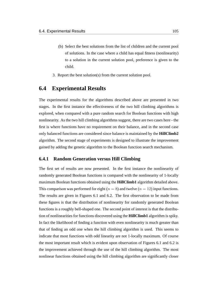
6.4. Experimental Results 105
(b) Select the best solutions from the list of children and the current pool
of solutions. In the case where a child has equal fitness (nonlinearity)
to a solution in the current solution pool, preference is given to the
child.
3. Report the best solution(s) from the current solution pool.
6.4 Experimental Results
The experimental results for the algorithms described above are presented in two
stages. In the first instance the effectiveness of the two hill climbing algorithms is
explored, when compared with a pure random search for Boolean functions with high
nonlinearity. As the two hill climbing algorithms suggest, there are two cases here - the
first is where functions have no requirement on their balance, and in the second case
only balanced functions are considered since balance is maintained by theHillClimb2
algorithm. The second stage of experiments is designed to illustrate the improvement
gained by adding the genetic algorithm to the Boolean function search mechanism.
6.4.1 Random Generation versus Hill Climbing
The first set of results are now presented. In the first instance the nonlinearity of
randomly generated Boolean functions is compared with the nonlinearity of 1-locally
maximum Boolean functions obtained using theHillClimb1 algorithm detailed above.
This comparison was performed for eight (n = 8) and twelve (n = 12) input functions.
The results are given in Figures 6.1 and 6.2. The first observation to be made from
these figures is that the distribution of nonlinearity for randomly generated Boolean
functions is a roughly bell-shaped one. The second point of interest is that the distribu-
tion of nonlinearities for functions discovered using theHillClimb1 algorithm is spiky.
In fact the likelihood of finding a function with even nonlinearity is much greater than
that of finding an odd one when the hill climbing algorithm is used. This seems to
indicate that most functions with odd linearity are not 1-locally maximum. Of course
the most important result which is evident upon observation of Figures 6.1 and 6.2 is
the improvement achieved through the use of the hill climbing algorithm. The most
nonlinear functions obtained using the hill climbing algorithm are significantly closer
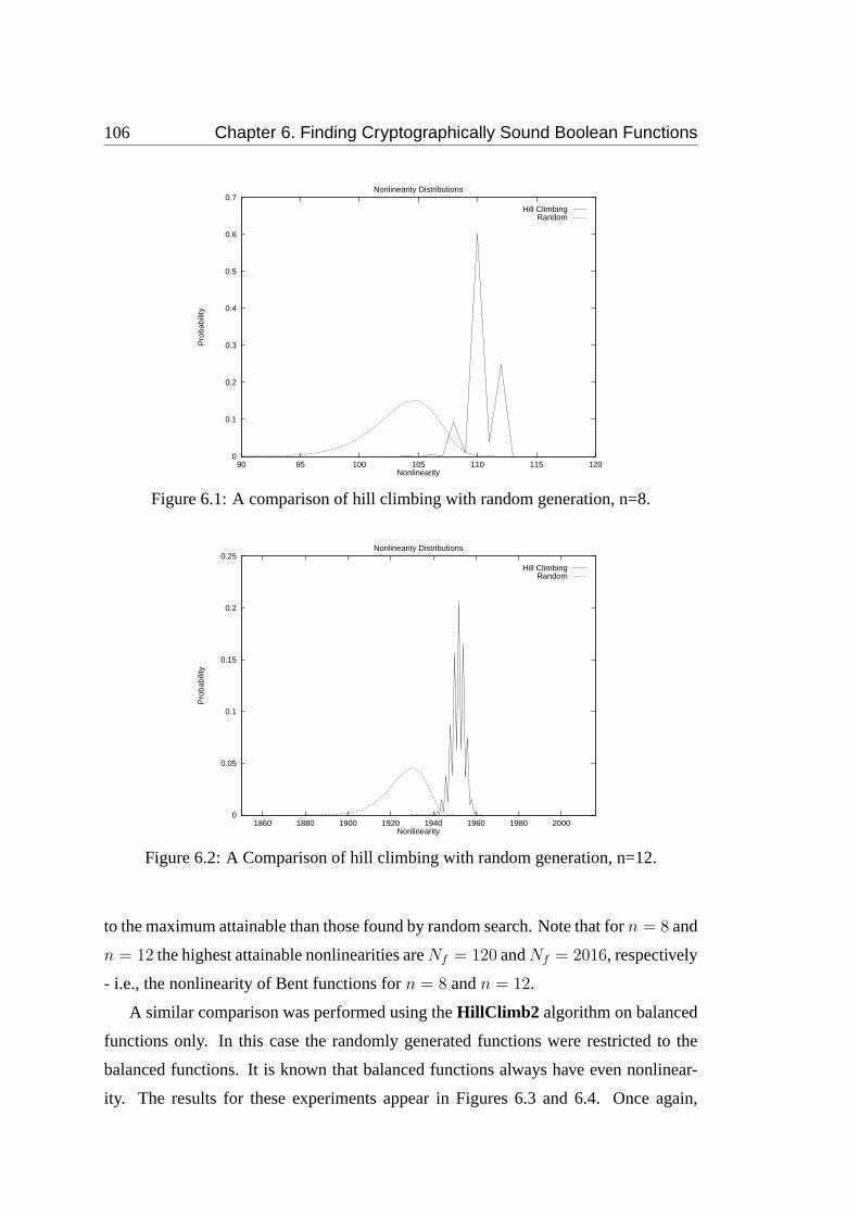
106 Chapter 6. Finding Cryptographically Sound Boolean Functions
0
0.1
0.2
0.3
0.4
0.5
0.6
0.7
90 95 100 105 110 115 120
Pro
babi
lity
Nonlinearity
Nonlinearity Distributions
Hill ClimbingRandom
Figure 6.1: A comparison of hill climbing with random generation, n=8.
0
0.05
0.1
0.15
0.2
0.25
1860 1880 1900 1920 1940 1960 1980 2000
Pro
babi
lity
Nonlinearity
Nonlinearity Distributions
Hill ClimbingRandom
Figure 6.2: A Comparison of hill climbing with random generation, n=12.
to the maximum attainable than those found by random search. Note that forn = 8 and
n = 12 the highest attainable nonlinearities areNf = 120 andNf = 2016, respectively
- i.e., the nonlinearity of Bent functions forn = 8 andn = 12.
A similar comparison was performed using theHillClimb2 algorithm on balanced
functions only. In this case the randomly generated functions were restricted to the
balanced functions. It is known that balanced functions always have even nonlinear-
ity. The results for these experiments appear in Figures 6.3 and 6.4. Once again,
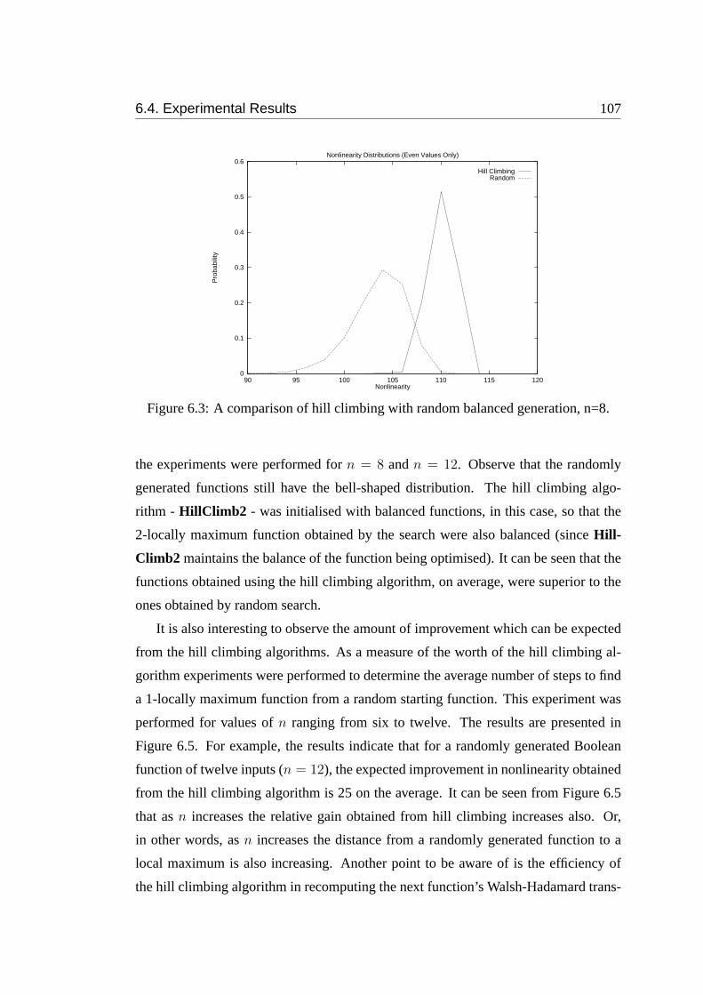
6.4. Experimental Results 107
0
0.1
0.2
0.3
0.4
0.5
0.6
90 95 100 105 110 115 120
Pro
babi
lity
Nonlinearity
Nonlinearity Distributions (Even Values Only)
Hill ClimbingRandom
Figure 6.3: A comparison of hill climbing with random balanced generation, n=8.
the experiments were performed forn = 8 andn = 12. Observe that the randomly
generated functions still have the bell-shaped distribution. The hill climbing algo-
rithm - HillClimb2 - was initialised with balanced functions, in this case, so that the
2-locally maximum function obtained by the search were also balanced (sinceHill-
Climb2 maintains the balance of the function being optimised). It can be seen that the
functions obtained using the hill climbing algorithm, on average, were superior to the
ones obtained by random search.
It is also interesting to observe the amount of improvement which can be expected
from the hill climbing algorithms. As a measure of the worth of the hill climbing al-
gorithm experiments were performed to determine the average number of steps to find
a 1-locally maximum function from a random starting function. This experiment was
performed for values ofn ranging from six to twelve. The results are presented in
Figure 6.5. For example, the results indicate that for a randomly generated Boolean
function of twelve inputs (n = 12), the expected improvement in nonlinearity obtained
from the hill climbing algorithm is 25 on the average. It can be seen from Figure 6.5
that asn increases the relative gain obtained from hill climbing increases also. Or,
in other words, asn increases the distance from a randomly generated function to a
local maximum is also increasing. Another point to be aware of is the efficiency of
the hill climbing algorithm in recomputing the next function’s Walsh-Hadamard trans-
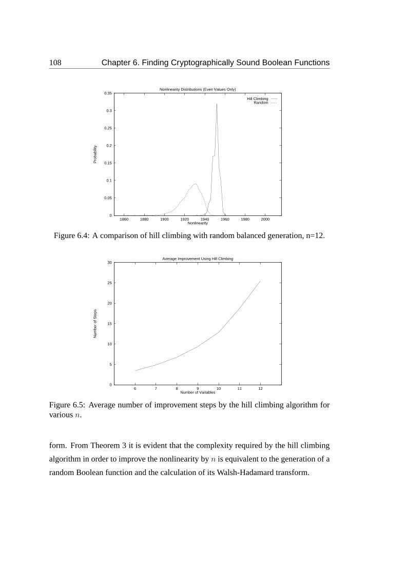
108 Chapter 6. Finding Cryptographically Sound Boolean Functions
0
0.05
0.1
0.15
0.2
0.25
0.3
0.35
1860 1880 1900 1920 1940 1960 1980 2000
Pro
babi
lity
Nonlinearity
Nonlinearity Distributions (Even Values Only)
Hill ClimbingRandom
Figure 6.4: A comparison of hill climbing with random balanced generation, n=12.
0
5
10
15
20
25
30
6 7 8 9 10 11 12
Num
ber
of S
teps
Number of Variables
Average Improvement Using Hill Climbing
Figure 6.5: Average number of improvement steps by the hill climbing algorithm forvariousn.
form. From Theorem 3 it is evident that the complexity required by the hill climbing
algorithm in order to improve the nonlinearity byn is equivalent to the generation of a
random Boolean function and the calculation of its Walsh-Hadamard transform.
6.4. Experimental Results 109
6.4.2 Genetic Algorithms with and without Hill Climbing
The second stage of experiments involve the genetic algorithm technique for finding
Boolean functions as described above. The experiments have shown that a genetic al-
gorithm with a pool size of less than 10 tends to converge too quickly, since a single
good solution comes to dominate the pool: it is the parent of many children that sur-
vive into subsequent generations. When both parent and offspring survive and breed,
their progeny tend to survive also, and that “family” soon dominates the gene pool,
producing convergence. A policy precluding “incest” counters this effect. This policy
may take the form of forbidding a parent pair from breeding if their Hamming distance
is too small, as set by some threshold parameter. However, when this parameter is set
too large, it prevents breeding by the best pairs, thus undermining the motivation for
the merge operation. Further experiments will be required to determine optimum sets
of genetic algorithm parameters. It is clear that to find very highly nonlinear functions,
larger pools are useful, since they converge less rapidly.
As an example of how the genetic algorithm performs, a single genetic algorithm
search was performed forn = 14 and the nonlinearity of the best function recorded at
the end of each iteration. Figure 6.6 is a plot of the results obtained for this particular
case, which compares the number of iterations against the best nonlinearity found thus
far. It can be seen that the most dramatic improvement in the nonlinearity occurs in the
early stages of the algorithm. After a certain number of iterations (approximately 40 in
this case) the rate of improvement in the nonlinearity decreases rapidly. In Figure 6.6
the solid line represents the nonlinearity of the best solution in the current pool and
the dotted line presents the average nonlinearity of all the functions currently in the
solution pool. After a while nearly all functions in the solution pool have the same
nonlinearity, indicating that the GA usually finds more than one function with the
highest nonlinearity.
The remaining results presented in this section are designed to illustrate the merits
of the genetic algorithm search over both random Boolean function generation and the
hill climbing algorithm,HillClimb1 . Note that in this section there is no requirement
of balance on the functions being generated.
As a benchmark the best results obtained from random search for functions with
inputs ranging from eight (n = 8) to sixteen (n = 16) were obtained for various search
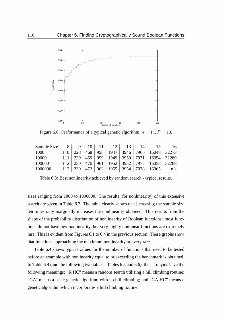
110 Chapter 6. Finding Cryptographically Sound Boolean Functions
7900
7920
7940
7960
7980
8000
8020
8040
0 20 40 60 80 100
Non
linea
rity
Number of Iterations
Figure 6.6: Performance of a typical genetic algorithm,n = 14, P = 10.
Sample Size 8 9 10 11 12 13 14 15 161000 110 228 468 958 1947 3946 7966 16048 3227310000 111 229 469 959 1949 3950 7971 16054 32280100000 112 230 470 961 1952 3952 7975 16058 322881000000 112 230 472 962 1955 3954 7978 16065 n/a
Table 6.3: Best nonlinearity achieved by random search - typical results.
sizes ranging from 1000 to 1000000. The results (for nonlinearity) of this extensive
search are given in Table 6.3. The table clearly shows that increasing the sample size
ten times only marginally increases the nonlinearity obtained. This results from the
shape of the probability distribution of nonlinearity of Boolean functions: most func-
tions do not have low nonlinearity, but very highly nonlinear functions are extremely
rare. This is evident from Figures 6.1 to 6.4 in the previous section. These graphs show
that functions approaching the maximum nonlinearity are very rare.
Table 6.4 shows typical values for the number of functions that need to be tested
before an example with nonlinearity equal to or exceeding the benchmark is obtained.
In Table 6.4 (and the following two tables - Tables 6.5 and 6.6), the acronyms have the
following meanings: “R HC” means a random search utilising a hill climbing routine;
“GA” means a basic genetic algorithm with no hill climbing; and “GA HC” means a
genetic algorithm which incorporates a hill climbing routine.
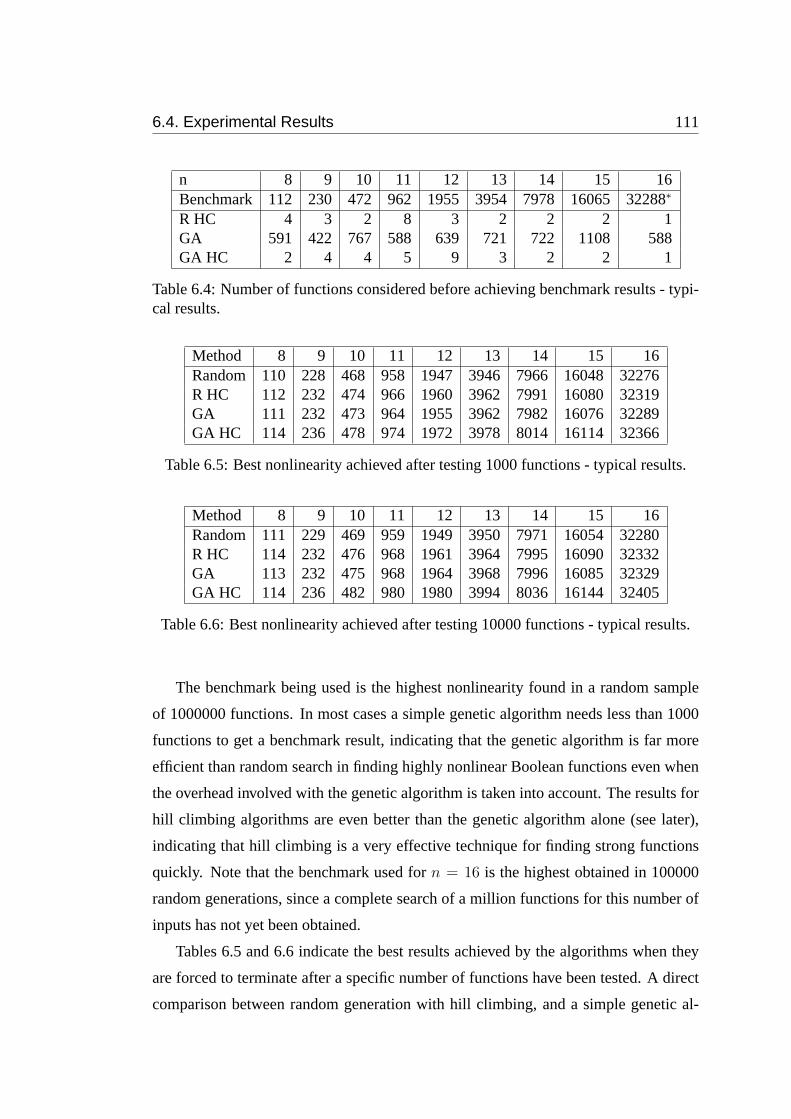
6.4. Experimental Results 111
n 8 9 10 11 12 13 14 15 16Benchmark 112 230 472 962 1955 3954 7978 16065 32288∗
R HC 4 3 2 8 3 2 2 2 1GA 591 422 767 588 639 721 722 1108 588GA HC 2 4 4 5 9 3 2 2 1
Table 6.4: Number of functions considered before achieving benchmark results - typi-cal results.
Method 8 9 10 11 12 13 14 15 16Random 110 228 468 958 1947 3946 7966 16048 32276R HC 112 232 474 966 1960 3962 7991 16080 32319GA 111 232 473 964 1955 3962 7982 16076 32289GA HC 114 236 478 974 1972 3978 8014 16114 32366
Table 6.5: Best nonlinearity achieved after testing 1000 functions - typical results.
Method 8 9 10 11 12 13 14 15 16Random 111 229 469 959 1949 3950 7971 16054 32280R HC 114 232 476 968 1961 3964 7995 16090 32332GA 113 232 475 968 1964 3968 7996 16085 32329GA HC 114 236 482 980 1980 3994 8036 16144 32405
Table 6.6: Best nonlinearity achieved after testing 10000 functions - typical results.
The benchmark being used is the highest nonlinearity found in a random sample
of 1000000 functions. In most cases a simple genetic algorithm needs less than 1000
functions to get a benchmark result, indicating that the genetic algorithm is far more
efficient than random search in finding highly nonlinear Boolean functions even when
the overhead involved with the genetic algorithm is taken into account. The results for
hill climbing algorithms are even better than the genetic algorithm alone (see later),
indicating that hill climbing is a very effective technique for finding strong functions
quickly. Note that the benchmark used forn = 16 is the highest obtained in 100000
random generations, since a complete search of a million functions for this number of
inputs has not yet been obtained.
Tables 6.5 and 6.6 indicate the best results achieved by the algorithms when they
are forced to terminate after a specific number of functions have been tested. A direct
comparison between random generation with hill climbing, and a simple genetic al-
112 Chapter 6. Finding Cryptographically Sound Boolean Functions
gorithm without hill climbing shows that these algorithms are about equally effective
for 1000 or 10000 function tests. Other experiments have suggested that as the com-
putation bound is increased, the performance of the genetic algorithm will eventually
exceed that of hill climbing. It is interesting to note that the best algorithm is clearly
a genetic algorithm with hill climbing. This hybrid algorithm is able to quickly obtain
functions far better than the benchmarks.
6.5 Summary
A cryptographic application of combinatorial optimisation has been proposed. It has
been shown in this chapter that the genetic algorithm is a powerful tool, when used in
combination with a simple hill climbing heuristic, for finding highly nonlinear Boolean
functions suitable for cryptographic applications. It is suggested that a similar tech-
nique could be used to find functions with other properties, or even a combination of
properties. Also, the technique could be extended to finding highly nonlinear substitu-
tion boxes.
The hill climbing technique exploits the properties of the Walsh-Hadamard trans-
form of the Boolean function in order to determine which bits of its truth table may be
complemented to improve the nonlinearity of the function. It is shown that the tech-
nique can be used to choose two different-valued bits to complement to improve the
nonlinearity while at the same time maintaining the function’s balance properties.
This technique is shown to be significantly superior to a random search. The ge-
netic algorithm can be seen to further improve the hill climbing technique allowing
functions which are even more nonlinear to be found.
This work could be extended to include an analysis of the algorithm to determine if
the bits selected for complementation can be chosen more carefully in order to extend
the number of steps the nonlinearity can take before a local maximum is achieved.
Chapter 7
Conclusions
This thesis has investigated the use of three well-studied optimisation heuristics - sim-
ulated annealing, the genetic algorithm and the tabu search - in the fields of automated
cryptanalysis of ciphers and automated Boolean function design. These fields are im-
portant to cryptologists since, for example, cryptographers designing ciphers need ac-
cess to Boolean functions satisfying an ever-growing list of criteria, while, on the other
hand, cryptanalysts need to process vast amounts of information in order to discover
and exploit the weaknesses in ciphers. As was demonstrated in the thesis, these three
techniques provide cryptographers and cryptanalysts with a tool which meets both of
these requirements.
There are two key issues to consider when considering the use of optimisation
heuristics. The first is to consider if a suitable solution evaluation mechanism exists.
As has been illustrated in this thesis, it is clear that a reliable and accurate assessment
technique must exist if the types of search heuristics used are to be of practical use. The
second issue to consider is to determine which technique is going to be most suitable.
This decision will be based upon the characteristics of the problem being solved and
the characteristics of each of the heuristics. For example, if a genetic algorithm is
being considered a suitable mating operation must be defined.
Understanding the limitations of optimisation techniques requires knowledge of
the characteristics associated with the problems which are typically being solved. The
theory of NP-completeness, which was discussed in Chapter 2 defines a class of prob-
lems which are known to be difficult to solve. Once convinced that large instances of
such problems are impossible to solveexactly, one quickly comes to realise the impor-
tance of approximate techniques such as the ones presented here. The large amount
113
114 Chapter 7. Conclusions
of research which has been, and still is being, carried out emphasises the power of
these techniques. The different characteristics of each of the optimisation techniques
considered in this work makes them suitable for different applications.
The classical ciphers generally have a very large number of possible keys and yet
they are relatively simple to cryptanalyse. This is because the encryption process does
not hide the statistics of the plaintext language. Knowledge of then-gram statistics for
the language (in this case English) allows the definition of a key assessment method
based upon then-gram statistics of the message decrypted with a proposed key. Once
a key assessment method is defined it is possible to implement a search algorithm
based on an optimisation heuristic. As was shown, these ciphers are especially vul-
nerable to automated attacks based on such techniques. This is the case since an at-
tacker can use these automated techniques to find a “close” approximation to the actual
key which may render the cryptogram readable, or, if not, partly readable. Heuristics
which utilised, separately, simulated annealing, the genetic algorithm and the tabu
search were designed and implemented in attacks on both the simple substitution ci-
pher and the transposition cipher. Overall, the tabu search was found to be the most
effective search heuristic when applied to the substitution and transposition ciphers.
The success of the tabu search can be attributed to its “memory” features which force
the search away from regions of the search space that have already been considered.
Simulated annealing and the genetic algorithm, which do not possess this feature, are
less efficient in their search of the key space. While all three techniques were found to
successfully cryptanalyse simple substitution ciphers and transposition ciphers, the ge-
netic algorithm is best suited to parallel implementations and because of the structure
of the polyalphabetic substitution cipher was the only technique applied to this cipher.
The parallel genetic algorithm approach to cryptanalysis of the polyalphabetic sub-
stitution cipher provides a linear improvement in complexity over traditional sequential-
type attacks since it can solve each of the separate keys simultaneously. Processing
nodes are able to share information about their keys so that any node can determine a
set of statistics based on how the message decrypts using those keys. This technique
was shown to work equally well for all polyalphabetic block sizes up to nine charac-
ters. It is suggested that, provided sufficient computing processors and ciphertext are
available, this attack would be successful on much larger block sizes as well.
115
A number of modifications to the fast correlation attack were proposed. Although
incorporating an optimisation heuristic (in this case simulated annealing) in the prob-
ability update stage does lead to some improvement over the original algorithm, it is
found that the fast resetting technique leads to even greater improvement. By resetting
the error probability vector after a fixed number of complementations of the recovered
keystream, a marked improvement in the attack is obtained. The fast resetting tech-
nique is shown to be superior to MacKay’s free energy minimisation method. This
result is based on extensive experiments with shift registers of various lengths.
This work could possibly be extended to include other types of stream ciphers.
Fast correlation attacks have been proposed on a large number of stream ciphers in-
cluding clock-controlled shift register based stream ciphers [29], the multiplexed gen-
erator [34] and the summation generator [66] (which incorporates memory - see Ap-
pendix B). Techniques similar to the ones discussed in this thesis could be modified to
possibly enhance the existing attacks.
The Merkle-Hellman public key cryptosystem utilises an NP-hard relative of the
NP-complete subset sum problem. Spillman’s method for attacking the Merkle-Hellman
system is shown to be flawed. The fitness function proposed by Spillman does not ac-
curately reflect how close a solution is to the correct one. An example is used to show
that it is possible to find a candidate solution whose fitness is within 0.01% of the fit-
ness of the correct solution and yet the candidate solution is different from the correct
solution in more than half of its bit positions. An additional problem with Spillman’s
approach is that the knapsack cryptosystem has only one solution. Traditionally, opti-
misation heuristics are applied when we are satisfied that the optimum solution cannot
be found but, instead, a “good” solution is sought. Applying a genetic algorithm to
a problem which is known to be NP-hard and which has only one correct solution
(among2n) can only be futile.
Based on the research presented in this thesis it could be concluded that optimisa-
tion heuristics show potential for use in the field of automated cryptanalysis. Although
rarely useful for completely cryptanalysing a cipher (except in the case of the classical
ciphers), these techniques have shown some promise when used to optimise existing
methods for attacking certain ciphers. Optimisation heuristics are proven performers
for problems which require searching a large solution space for solutions with “good”
116 Chapter 7. Conclusions
characteristics (rather than the “best” solution). One possible example for further re-
search in this area is searching forcharacteristicsfor use in differential, or linear crypt-
analysis. Matsui has proposed a branch-and-bound search for this purpose, and it is
possible that another optimisation heuristic may be more efficient for such a purpose.
The branch-and-bound approach is sufficient to find characteristics for DES; however,
characteristics for ciphers which utilise larger S-boxes (such as CAST – [1]) may be
better determined using an optimisation technique such as the ones discussed in this
thesis.
In addition to their application to the field of cryptanalysis, optimisation heuristics
have also proven to be useful for cryptographic applications.
A technique for determining “neighbours” of a given function which have higher
nonlinearity is introduced. This approach can be used iteratively in order to find a
Boolean function which is locally maximum in nonlinearity, in the sense that comple-
menting any one of the bits in its truth table will not lead to a function with higher
nonlinearity. In addition to nonlinearity, balance is one of the fundamental proper-
ties required of cryptographically sound Boolean functions. A technique is presented
which allows the search to determine two differently-valued truth table positions such
that complementing each of these (binary) values increases the overall nonlinearity of
the function and at the same time maintains its balance. Thus, the techniques can be
used to either improve both nonlinearity and balance of a non-balanced function, or
to improve nonlinearity while maintaining the balance of a function. Incorporating
this technique in a genetic algorithm is shown to produce a search which reliably finds
functions with higher nonlinearity than other techniques.
This cryptographic application for optimisation heuristics is open to a number of
extensions in future work. Similar techniques could be used to determine highly non-
linear S-boxes. Also, many other cryptographically desirable properties of Boolean
functions are known. These techniques, or similar ones, could be used to find func-
tions satisfying other cryptographic criteria, or (ideally) a combination of a number of
criteria. This would be an especially useful extension since several cryptographic prop-
erties are known to conflict so that the “best” function is based on a trade-off between
a number of properties.
A number of applications of optimisation heuristics to the field of cryptology have

117
been presented. The optimisation heuristics do not work for all applications and it is
important to be aware of this. Once the limitations of these techniques are understood
it becomes clear which applications will gain the most benefit from an approach based
on them. The examples provided in this thesis, along with suggestions of further ap-
plications, are intended to increase others’ awareness of optimisation heuristics as a
useful tool in cryptology, and to assist in understanding when and when not they are
best utilised.

118 Chapter 7. Conclusions
Appendix A
Classical Ciphers
In this appendix three different classical ciphers - the simple substitution cipher, the
polyalphabetic substitution cipher and the transposition cipher - are described. In each
case an example is given to illustrate the usage of the cipher. Properties of each of the
ciphers which are utilised in their cryptanalysis are also discussed.
Several variations of substitution and transposition ciphers exist. The ones pre-
sented here are the most general. Most historical cases of the substitution cipher are
just specific instances of the general cases described in the following two sections (ex-
amples are the Caesar, Vigenere and Beaufort ciphers - see [35] or [4]).
A.1 Simple Substitution Ciphers
The simple substitution cipher (sometimes referred to as the monoalphabetic substitu-
tion cipher to distinguish it from the polyalphabetic substitution cipher which is pre-
sented in Section A.2) is the most simple of substitution ciphers. Each symbol in the
plaintext maps to a (usually different) symbol in the ciphertext. The processes of en-
cryption and decryption are best described with an example, such as the one following.
Example A.1 A simple substitution cipher key can be represented as a permutation of
the plaintext alphabet. Table A.1 gives a sample key. Using this representation theith
letter in the plaintext alphabet is encrypted to theith element of the key. The string
“ . . .the money is in a locker at the airport. . .” is encrypted using the key in the table
(see Table A.1).
Using the key representation in Table A.1, the original message can be discovered
119
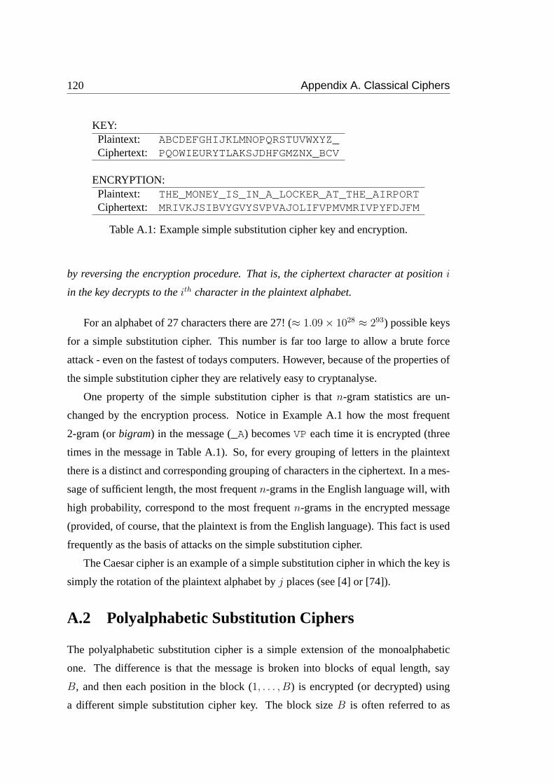
120 Appendix A. Classical Ciphers
KEY:Plaintext: ABCDEFGHIJKLMNOPQRSTUVWXYZ_Ciphertext: PQOWIEURYTLAKSJDHFGMZNX_BCV
ENCRYPTION:Plaintext: THE_MONEY_IS_IN_A_LOCKER_AT_THE_AIRPORTCiphertext: MRIVKJSIBVYGVYSVPVAJOLIFVPMVMRIVPYFDJFM
Table A.1: Example simple substitution cipher key and encryption.
by reversing the encryption procedure. That is, the ciphertext character at positioni
in the key decrypts to theith character in the plaintext alphabet.
For an alphabet of 27 characters there are 27! (≈ 1.09× 1028 ≈ 293) possible keys
for a simple substitution cipher. This number is far too large to allow a brute force
attack - even on the fastest of todays computers. However, because of the properties of
the simple substitution cipher they are relatively easy to cryptanalyse.
One property of the simple substitution cipher is thatn-gram statistics are un-
changed by the encryption process. Notice in Example A.1 how the most frequent
2-gram (orbigram) in the message (_A) becomesVP each time it is encrypted (three
times in the message in Table A.1). So, for every grouping of letters in the plaintext
there is a distinct and corresponding grouping of characters in the ciphertext. In a mes-
sage of sufficient length, the most frequentn-grams in the English language will, with
high probability, correspond to the most frequentn-grams in the encrypted message
(provided, of course, that the plaintext is from the English language). This fact is used
frequently as the basis of attacks on the simple substitution cipher.
The Caesar cipher is an example of a simple substitution cipher in which the key is
simply the rotation of the plaintext alphabet byj places (see [4] or [74]).
A.2 Polyalphabetic Substitution Ciphers
The polyalphabetic substitution cipher is a simple extension of the monoalphabetic
one. The difference is that the message is broken into blocks of equal length, say
B, and then each position in the block (1, . . . , B) is encrypted (or decrypted) using
a different simple substitution cipher key. The block sizeB is often referred to as
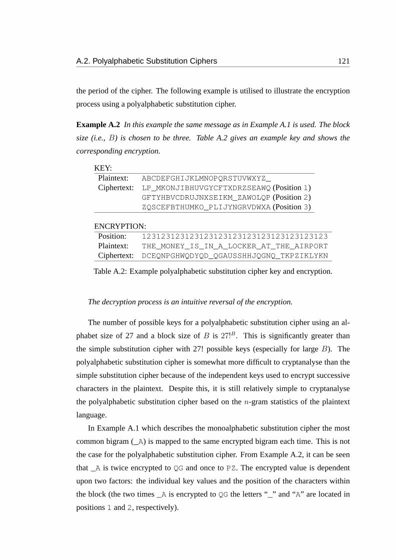
A.2. Polyalphabetic Substitution Ciphers 121
the period of the cipher. The following example is utilised to illustrate the encryption
process using a polyalphabetic substitution cipher.
Example A.2 In this example the same message as in Example A.1 is used. The block
size (i.e.,B) is chosen to be three. Table A.2 gives an example key and shows the
corresponding encryption.
KEY:Plaintext: ABCDEFGHIJKLMNOPQRSTUVWXYZ_Ciphertext: LP_MKONJIBHUVGYCFTXDRZSEAWQ(Position1)
GFTYHBVCDRUJNXSEIKM_ZAWOLQP(Position2)ZQSCEFBTHUMKO_PLIJYNGRVDWXA(Position3)
ENCRYPTION:Position: 123123123123123123123123123123123123123Plaintext: THE_MONEY_IS_IN_A_LOCKER_AT_THE_AIRPORTCiphertext: DCEQNPGHWQDYQD_QGAUSSHHJQGNQ_TKPZIKLYKN
Table A.2: Example polyalphabetic substitution cipher key and encryption.
The decryption process is an intuitive reversal of the encryption.
The number of possible keys for a polyalphabetic substitution cipher using an al-
phabet size of 27 and a block size ofB is 27!B. This is significantly greater than
the simple substitution cipher with 27! possible keys (especially for largeB). The
polyalphabetic substitution cipher is somewhat more difficult to cryptanalyse than the
simple substitution cipher because of the independent keys used to encrypt successive
characters in the plaintext. Despite this, it is still relatively simple to cryptanalyse
the polyalphabetic substitution cipher based on then-gram statistics of the plaintext
language.
In Example A.1 which describes the monoalphabetic substitution cipher the most
common bigram (_A) is mapped to the same encrypted bigram each time. This is not
the case for the polyalphabetic substitution cipher. From Example A.2, it can be seen
that _A is twice encrypted toQGand once toPZ. The encrypted value is dependent
upon two factors: the individual key values and the position of the characters within
the block (the two times_A is encrypted toQGthe letters “_” and “A” are located in
positions1 and2, respectively).
122 Appendix A. Classical Ciphers
The Vigenere and Beaufort ciphers are examples of polyalphabetic substitution
ciphers (see [4] for descriptions).
Any attack on the polyalphabetic substitution cipher must involve determining the
period as well as decrypting the ciphertext. Usually the task of determining the pe-
riod is performed separately and prior to the message recovery phase. Methods for
determining the period are now discussed.
A.2.1 Determining the Period of a Polyalphabetic Cipher
A number of methods for determining the block length (or period) have been reported
in the literature. Two such methods are now described briefly.
Friedman [19] discovered that theIndex of Coincidence(IC) (see also [4]) can be
used to give a general indication of the period of a polyalphabetic substitution cipher.
Given an intercepted ciphertext message of lengthK, the index of coincidence is given
by Equation A.1 wherefλ denotes the frequency of characterλ in the ciphertext.
IC =
∑λ∈C fλ(fλ − 1)
K(K − 1)(A.1)
A discussion of the theory of the IC is given in [19] and does not fall into the scope
of this work. However, it can be shown that the IC and the period of a cipher are
related and, providingK is sufficiently large, the IC can be used to give a reasonable
indication of the block length,B. The IC can also be used to support the findings of
another method, especially when more than one period is indicated by that method.
The second technique discussed here is theKasiskitest devised by Kasiski in 1863
(see [4]). In an encrypted message produced by a polyalphabetic substitution cipher, a
particular sequence of characters may be repeated a number of times. It is highly likely
(although not certain) that the repeated sequence will represent the same plaintext. In
the case that the repeated sequence does represent the same plaintext, the distance be-
tween the two instances of the sequence will give an indication of the period of the
cipher. All of the prime factors of the distance between the two instance are possi-
bilities for the period of the cipher. If there are a number of different sequences in
the cryptogram which are repeated, or if a particular sequence is repeated many times,
then by finding the factors of all the distances between them, a good indication of the
period can be obtained.
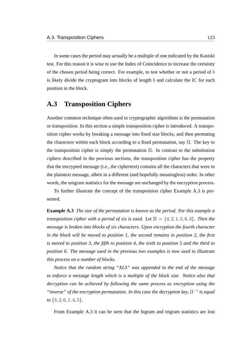
A.3. Transposition Ciphers 123
In some cases the period may actually be a multiple of one indicated by the Kasiski
test. For this reason it is wise to use the Index of Coincidence to increase the certainty
of the chosen period being correct. For example, to test whether or not a period ofb
is likely divide the cryptogram into blocks of lengthb and calculate the IC for each
position in the block.
A.3 Transposition Ciphers
Another common technique often used in cryptographic algorithms is the permutation
or transposition. In this section a simple transposition cipher is introduced. A transpo-
sition cipher works by breaking a message into fixed size blocks, and then permuting
the characters within each block according to a fixed permutation, sayΠ. The key to
the transposition cipher is simply the permutationΠ. In contrast to the substitution
ciphers described in the previous sections, the transposition cipher has the property
that the encrypted message (i.e., the ciphertext) contains all the characters that were in
the plaintext message, albeit in a different (and hopefully meaningless) order. In other
words, the unigram statistics for the message are unchanged by the encryption process.
To further illustrate the concept of the transposition cipher Example A.3 is pre-
sented.
Example A.3 The size of the permutation is known as the period. For this example a
transposition cipher with a period of six is used. LetΠ = {4, 2, 1, 5, 6, 3}. Then the
message is broken into blocks of six characters. Upon encryption the fourth character
in the block will be moved to position 1, the second remains in position 2, the first
is moved to position 3, the fifth to position 4, the sixth to position 5 and the third to
position 6. The message used in the previous two examples is now used to illustrate
this process on a number of blocks.
Notice that the random string “XLS” was appended to the end of the message
to enforce a message length which is a multiple of the block size. Notice also that
decryption can be achieved by following the same process as encryption using the
“inverse” of the encryption permutation. In this case the decryption key,Π−1 is equal
to {3, 2, 6, 1, 4, 5}.
From Example A.3 it can be seen that the bigram and trigram statistics are lost
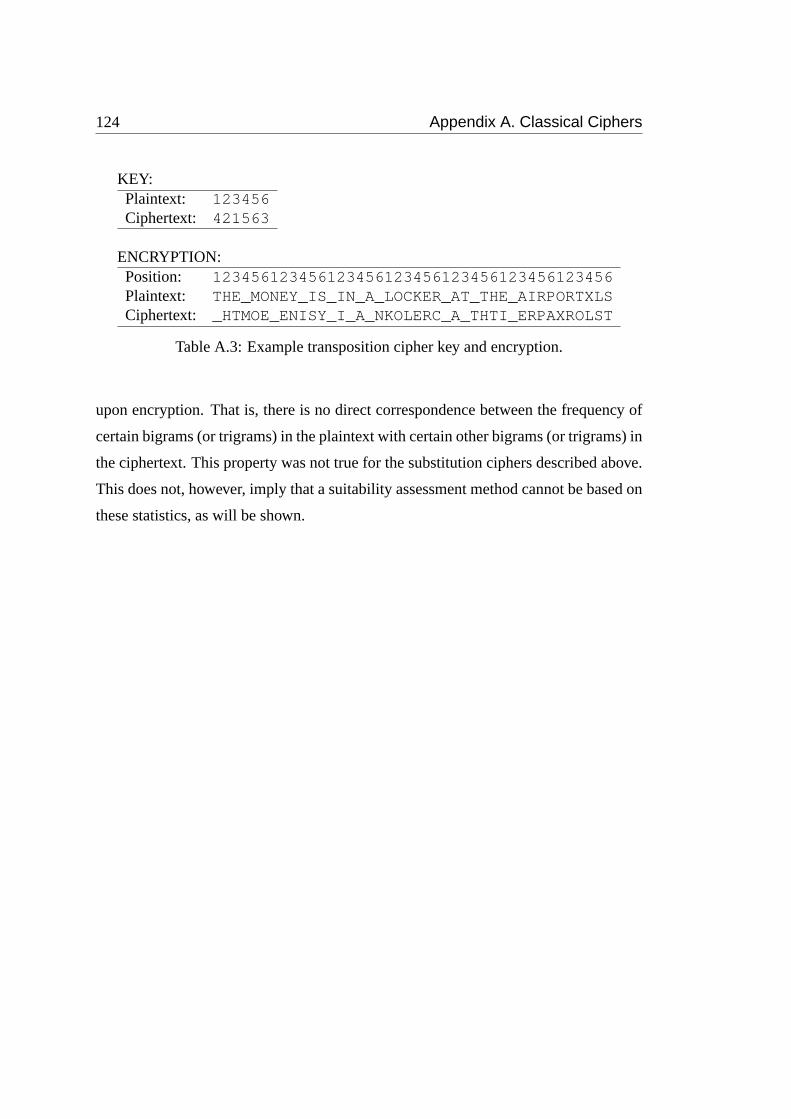
124 Appendix A. Classical Ciphers
KEY:Plaintext: 123456Ciphertext: 421563
ENCRYPTION:Position: 123456123456123456123456123456123456123456Plaintext: THE_MONEY_IS_IN_A_LOCKER_AT_THE_AIRPORTXLSCiphertext: _HTMOE_ENISY_I_A_NKOLERC_A_THTI_ERPAXROLST
Table A.3: Example transposition cipher key and encryption.
upon encryption. That is, there is no direct correspondence between the frequency of
certain bigrams (or trigrams) in the plaintext with certain other bigrams (or trigrams) in
the ciphertext. This property was not true for the substitution ciphers described above.
This does not, however, imply that a suitability assessment method cannot be based on
these statistics, as will be shown.
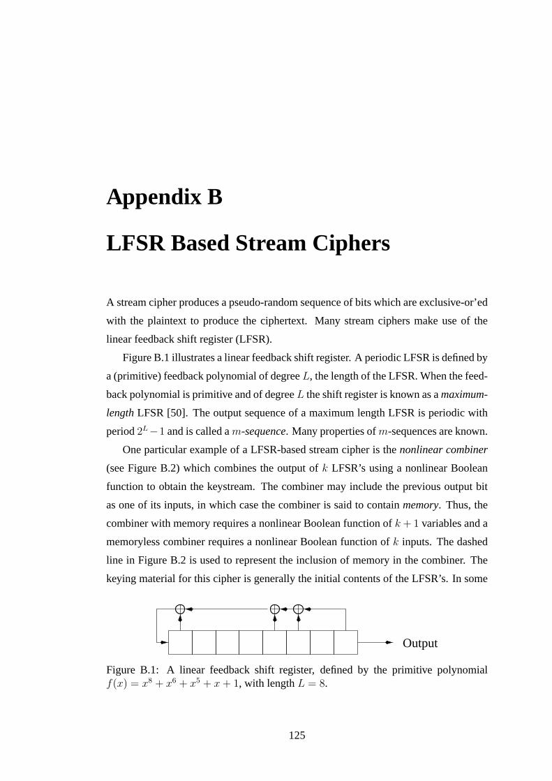
Appendix B
LFSR Based Stream Ciphers
A stream cipher produces a pseudo-random sequence of bits which are exclusive-or’ed
with the plaintext to produce the ciphertext. Many stream ciphers make use of the
linear feedback shift register (LFSR).
Figure B.1 illustrates a linear feedback shift register. A periodic LFSR is defined by
a (primitive) feedback polynomial of degreeL, the length of the LFSR. When the feed-
back polynomial is primitive and of degreeL the shift register is known as amaximum-
lengthLFSR [50]. The output sequence of a maximum length LFSR is periodic with
period2L−1 and is called am-sequence. Many properties ofm-sequences are known.
One particular example of a LFSR-based stream cipher is thenonlinear combiner
(see Figure B.2) which combines the output ofk LFSR’s using a nonlinear Boolean
function to obtain the keystream. The combiner may include the previous output bit
as one of its inputs, in which case the combiner is said to containmemory. Thus, the
combiner with memory requires a nonlinear Boolean function ofk + 1 variables and a
memoryless combiner requires a nonlinear Boolean function ofk inputs. The dashed
line in Figure B.2 is used to represent the inclusion of memory in the combiner. The
keying material for this cipher is generally the initial contents of the LFSR’s. In some
Output
Figure B.1: A linear feedback shift register, defined by the primitive polynomialf(x) = x8 + x6 + x5 + x + 1, with lengthL = 8.
125
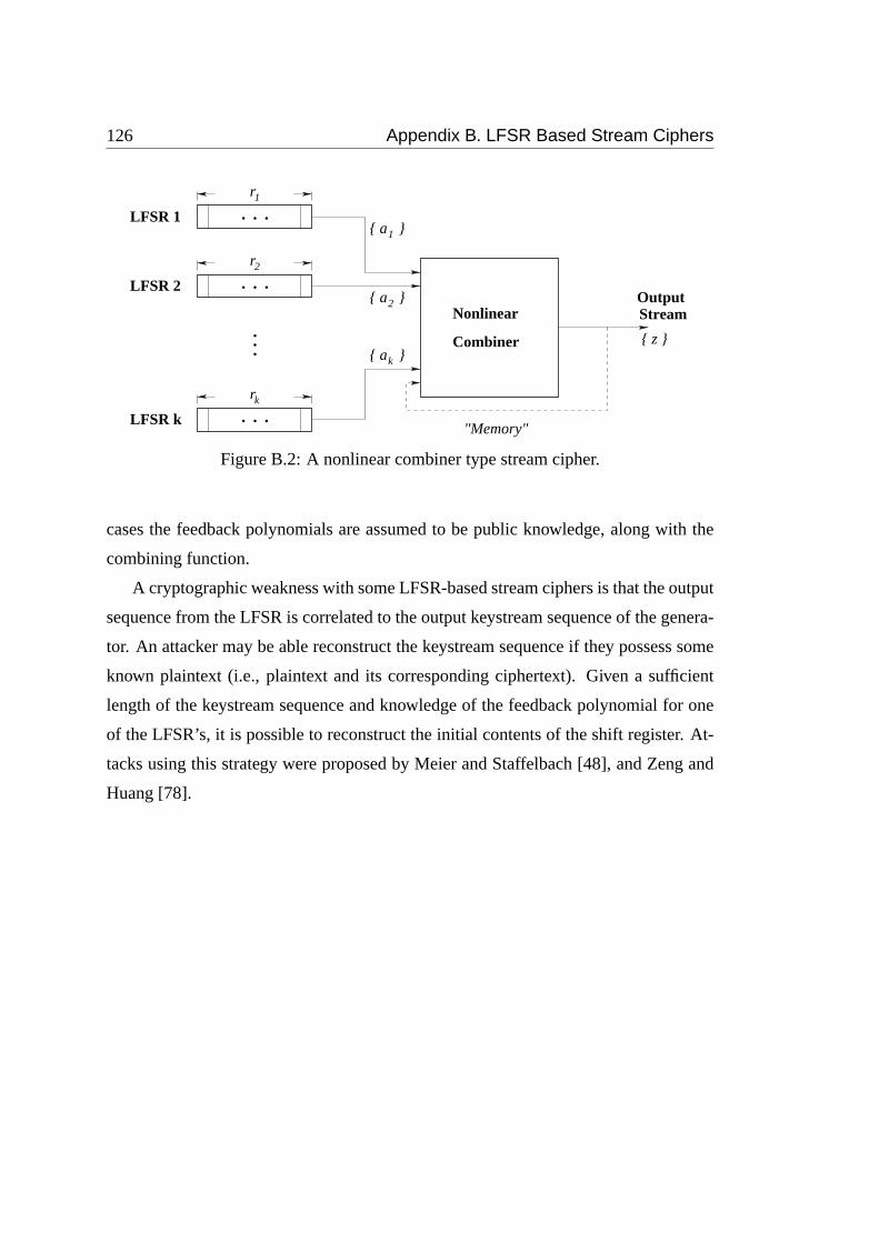
126 Appendix B. LFSR Based Stream Ciphers
LFSR 2 . . .r2
Combiner
Nonlinear StreamOutput
"Memory"
{ z }
{ a }2
{ a }1
LFSR 1 . . .r1
{ a }k
. . .rk
LFSR k
...
Figure B.2: A nonlinear combiner type stream cipher.
cases the feedback polynomials are assumed to be public knowledge, along with the
combining function.
A cryptographic weakness with some LFSR-based stream ciphers is that the output
sequence from the LFSR is correlated to the output keystream sequence of the genera-
tor. An attacker may be able reconstruct the keystream sequence if they possess some
known plaintext (i.e., plaintext and its corresponding ciphertext). Given a sufficient
length of the keystream sequence and knowledge of the feedback polynomial for one
of the LFSR’s, it is possible to reconstruct the initial contents of the shift register. At-
tacks using this strategy were proposed by Meier and Staffelbach [48], and Zeng and
Huang [78].
Appendix C
The Merkle-Hellman Public KeyCryptosystem
Merkle and Hellman (in [51]) proposed their “knapsack” cipher in 1978. The term
“knapsack” is a misnomer because the security of the cryptosystem is based on the
difficulty of solving the subset sum problem, rather than the closely related knapsack
problem. Since their pioneering work, many cryptosystems based on the difficulty of
solving the same problem have been proposed.
Thesubset sumproblem (which is defined in [22] and known to be NP-complete)
can be expressed as follows: “GivenA = {a1, a2, . . . , an} a finite set of positive
integers, andB a positive integer, is there a subsetA′ ⊆ A such that the sum of the
sizes of the elements inA′ is exactlyB?” To break the Merkle-Hellman cryptosystem
by attacking the encryption process rather than the structure of the secret key, one has
to solve the following related NP-hard problem: “GivenA = {a1, a2, . . . , an} a finite
set of positive integers, andB a positive integer, find the subsetA′ ⊆ A such that the
sum of the sizes of the elements inA′ is exactlyB (given thatA′ exists).”
In the Merkle-Hellman cipher the public key is the setA and the finite field modu-
lus,p. The public keyA is formed by multiplying each element of a super-increasing
sequence by a secret multiplier,w, and reducing modulop, where gcd(w, p) = 1. The
secret key is the super-increasing sequence and the secret multiplier,w. In general the
public keyA will be randomly distributed elements. Encryption is performed onn bit
binary blocks by summing the elements inA which correspond to a1 in the plaintext
block. Typicallyw andp would be very large numbers andn should be sufficiently
large to prevent an exhaustive search of the solution space. The following example
127

128 Appendix C. The Merkle-Hellman Public Key Cryptosystem
describes the operations of generating a public/private key pair for a knapsack cipher
and gives an example of the encryption and decryption processes.
Example C.1 Suppose Alice wishes to establish a knapsack public/private key pair.
The key pair is generated using, in this case, the parametersn = 8, the knapsack size,
w = 500, the secret multiplier andp = 711 the public modulus. A super-increasing
sequenceS = { 2, 5, 11, 20, 41, 85, 211, 463} is chosen to form part of the secret key
(S andw together constitute the secret key). The public part of the key is made up ofp,
the modulus, and the setA obtained by multiplying the elements ofS with w modulop.
In this instanceA = { 289, 367, 523, 46, 592, 551, 272, 425}. A andp are published
as the public key for Alice.
Now suppose Bob wishes to send Alice an encrypted message. Binary messages
are encoded inn bit blocks. A block of Bob’s message is as follows:M = { 0, 1,
0, 1, 1, 1, 0, 1}. The ciphertext,C, is computed fromA and p as follows: C =
(∑n
i=1 aimi) mod p whereA = {a1, a2, . . . , an} andM = {m1,m2, . . . , mn}. Thus
Bob’s ciphertext will be:C = 367+46+592+551+425 mod 711 = 1981 mod 711 =
559. Bob sendsC = 559 to Alice.
Alice wishes to decode Bob’s message. Alice’s first step is to multiply the cipher-
text by the inverse of the secret multiplier (w−1) modulop. Here w−1 = 155 and
Cw−1 mod p = 559 × 155 mod 711 = 614. It is then trivial for Alice to decode the
message by determining the elements ofS which add to give 614. For example, Alice
can repeatedly subtract the largest possible value ofS from the ciphertext until a value
of zero results. The values fromS used in the subtraction will correspond to 1’s in the
decrypted message block.
The Merkle-Hellman cryptosystem was broken by Shamir [68] (and others) in the
early 1980’s. Details of the attack are given below. The problem with most knapsack-
type cryptosystems is that the public key does not properly hide the structure of the
secret key.
C.1. A review of Attacks on the Merkle-Hellman Cryptosystem 129
C.1 A review of Attacks on the Merkle-Hellman Cryp-tosystem
In this section some of the theoretical aspects of attacks on knapsack-type ciphers
are presented. The analysis given here follows the description given in [70], however
several attacks were presented around 1982 by Brickell [7], Shamir [68] and Desmedt
et al [15].
In accordance with the notation above,S = {s1, s2, . . . , sn} represents the super-
increasing sequence which, together with the secret multiplier,w, comprises the secret
portion of the public key cryptosystem.
Recall that the public key portion comprises the setA = {a1, a2, . . . , an} and the
modulus,p. Each element ofA is obtained using the relation
ai = w × si mod p.
Then, ifw−1 is the modular inverse ofw,
si = w−1 × ai − p× ki,
and wheni = 1
s1 = w−1 × a1 − p× k1.
Multiplying the first of these byb1 and the second bybi and subtracting one from the
other gives
ai × k1 − a1 × ki = (a1 × si − ai × s1)/p
Now, sincep > s1 + s2 + . . . sn, ai < p ands1 < si, we have
a1 × si − ai × s1 > a1 × si − p× s1
> a1 × si − p× si
> (a1 − p)× si
> −p× si
and hence
|ai × k1 − a1 × ki| < p× si/(a1 + a2 + . . . + an).

130 Appendix C. The Merkle-Hellman Public Key Cryptosystem
A property of the super-increasing sequence is that
si+j ≥ 2j−1 × (si + 1),
or, expressed differently,
(si + 1)/si+j ≤ 21−j.
Whenj = n− i it follows that
(si + 1)/sn ≤ 2i+1−n
and thus
si/(s1 + s2 + . . . + sn) < (si + 1)/sn ≤ 2i+1−n.
Therefore
|ai × k1 − a1 × ki| < p× 2i+1−n
and, dividing byki × ai,
|k1/ki − a1/a1| < p× 2i+1−n/(ki × ai)
< p× 2i+1−n/ai.
This results shows that theki are not random and can be determined using the
above inequalities ifp is known. Shamir showed that the final inequality can be solved
using an algorithm proposed by Lenstra [39]. This attack can be used to determine the
ki in polynomial time and hence the Merkle-Hellman cryptosystem is broken easily.
This attack can be used on all similar cryptosystems based on disguising a secret trap-
door sequence (in the case of the Merkle-Hellman cryptosystem, the super-increasing
sequenceS is the trapdoor).
Appendix D
Boolean Functions and theirCryptographic Properties
This appendix provides an introduction to Boolean functions: their representation, op-
erators and properties.
The most basic representation of a Boolean function is by its binary truth table.
The binary truth tableof a Boolean function ofn variables is denotedf(x) where
f(x) ∈ {0, 1} andx = {x1, x2, . . . , xn}, xi ∈ {0, 1}, i = 1, . . . , n. The truth table
contains2n elements corresponding to all possible combinations of then binary inputs.
Sometimes it is desirable to consider a Boolean function over the set{1,−1} rather
than {0, 1}. The polarity truth tableof a Boolean function is denotedf(x) where
f(x) ∈ {1,−1} andf(x) = (−1)f(x) = 1 − 2f(x). Thus whenf(x) = 1 it follows
that f(x) = −1. It is also important to note that XOR (exclusive or) over{0, 1} is
equivalent to real multiplication over{1,−1}. Thus,
h(x) = f(x)⊕ g(x)
⇒ h(x) = f(x)g(x).
Two fundamental properties of Boolean functions are Hamming weight and Ham-
ming distance. TheHamming weightof a Boolean function is the number of ones in
the binary truth table, or equivalently the number of−1s in the polarity truth table.
That is, the Hamming weight of a Boolean function, hwt(f), is given by:
hwt(f) =∑x
f(x)
=1
2
(2n −∑
x
f(x)
).
131
132 Appendix D. Boolean Functions and their Cryptographic Properties
TheHamming distancebetween two Boolean functions is the number of positions
in which their truth tables differ. The Hamming distance between two Boolean func-
tions, dist(f, g), can be calculated from either the binary truth table or the polarity truth
table as follows:
dist(f, g) =∑x
(f(x)⊕ g(x))
=1
2
(2n −∑
x
(f(x)g(x)
).
How well two Boolean functions correlate is also of interest. The correlation be-
tween two Boolean functions,c(f, g), gives an indication of the extent to which two
functions approximate each other. The correlation is a real number in the range [-1,1]
and is given by:
c(f, g) = 1− dist(f, g)
2n−1
= 2−n∑x
f(x)g(x).
Complementing one of the Boolean functions truth tables does not alter the magnitude
of the correlation between the two functions.
For cryptographic Boolean functions it is usually desired that there are an equal
number of 0’s and 1’s in the binary truth table. When this is the case the function
is said to bebalanced. Balance is a primary cryptographic criterion: an imbalanced
function has sub-optimum unconditional entropy (i.e., it is correlated to a constant
function). The imbalance of a Boolean function is defined as:
If =1
2|∑
x
f(x)|
= 2n−1|c(f, 0)|,
where0 denotes the constant zero Boolean function. The magnitude of the correlation
between a function and the constant zero function is simplyIf
2n−1 . A function with zero
imbalance is balanced and has no correlation to the constant functions.
A linear function,Lω(x), selected byω ∈ Zn2 is defined:
Lω(x) = ω · x= ω1x1 ⊕ ω2x2 ⊕ · · · ⊕ ωnxn.
133
An affinefunction is one of the form
Aω(x) = ω · x⊕ c,
wherec ∈ Z2.
The Hamming distance to linear functions is an important cryptographic property,
since ciphers that employ nearly linear functions can be broken easily by a variety of
methods (for example see [43, 27]). In particular, both differential and linear cryptanal-
ysis techniques [5, 44] are resisted by highly nonlinear functions. Thus the minimum
distance to any affine function is an important indicator of the cryptographic strength
of a Boolean function.
Thenonlinearityof a Boolean function is this minimum distance, or the distance to
the set of affine functions. Note that complementing a Boolean function’s binary truth
table will not change the nonlinearity, so the magnitude of the correlation to all linear
functions, of which there are2n, must be considered.
The Hamming distance between a pair of functions can be determined by evalu-
ating both functions for all inputs and counting the disagreements. This process has
complexityO(2n). It follows that determining the nonlinearity in this naive fashion
will require O(22n) function evaluations, which is infeasible even for smalln. How-
ever, a tool exists that enables the calculation of all linear correlation coefficients in
O(n2n) operations. This is the fast Walsh-Hadamard Transform (denotedF (ω)), and
its uses in cryptography and elsewhere are well known [3, 77]. The Walsh-Hadamard
Transform (WHT) of a Boolean function is defined as:
F (ω) =∑x
f(x)Lω(x).
It is clear from this definition that the value ofF (ω) is closely related to the Hamming
distance betweenf(x) and the linear functionLω(x). In fact the correlation to the
linear function is given byc(f, Lω) = F (ω)2n .
The nonlinearity,Nf , of f(x) is related to the maximum magnitude of WHT values
WHMAX and is given by:
Nf =1
2∗ (2n −WHMAX ).
Clearly in order to increase the nonlinearity, WHMAX must be decreased. A function
is uncorrelated with linear functionLω(x) when F (ω) = 0. Cryptographically, it
134 Appendix D. Boolean Functions and their Cryptographic Properties
would be desirable to find Boolean functions which have all WHT values equal to
zero, since such functions have no correlation to any affine functions. However, it is
known [49] that such functions do not exist. A well known theorem, widely attributed
to Parseval [41], states that the sum of the squares of the WHT values is the same
constant for every Boolean function:∑
ω F 2(ω) = 22n. Thus a tradeoff exists in
minimising affine correlation. When a function is altered so that its correlation to some
affine function is reduced, the correlation to some other affine function is increased.
It is known that the Bent functions [65] satisfy the property that|F (ω)| = 2n2 for
all ω. Bent functions exist only for evenn, and they attain the maximum possible
nonlinearity ofNBENT = 2n−1 − 2n2−1. Note, however, that Bent functions are not bal-
anced. It is an open problem to determine an expression for the maximum nonlinearity
of functions with an odd number of inputs. It is known that, forn odd, it is possible
to construct a function with nonlinearity2n−1−2n−1
2 by concatenating Bent functions.
It is known that forn = 3, 5, 7 that this is in fact the upper bound of nonlinearity.
The only value ofn for which it is known that this value is not the upper bound is
n = 15 [58, 59].
Bibliography
[1] C. Adams and S.E. Tavares. Designing S-boxes for ciphers resistant to differential
cryptanalysis. In W. Wolfowicz, editor,Proceedings of the 3rd Symposium on
State and Progress of Research in Cryptography, pages 181–190, Rome, Italy,
1993.
[2] J. Wesley Barnes and Manuel Laguna. A tabu search experience in production
scheduling.Annals of Operations Research, 41:141–156, 1993.
[3] K.G. Beauchamp.Applications of Walsh and Related Functions. Academic Press,
1984.
[4] Henry Beker and Fred Piper.Cipher Systems: The Protection of Communica-
tions. Wiley-Interscience, London, 1982.
[5] E. Biham and A. Shamir. Differential cryptanalysis of DES-like cryptosystems.
In Advances in Cryptology - Crypto ’90, Proceedings, LNCS, volume 537, pages
2–21. Springer-Verlag, 1991.
[6] Paulo Brandimarte. Routing and scheduling in a flexible job shop by tabu search.
Annals of Operations Research, 41:157–183, 1993.
[7] E.F. Brickell. Solving low density knapsacks. InAdvances in Cryptology: Pro-
ceedings of CRYPTO ’83, pages 25–37, 1984.
[8] Donald E. Brown, Christopher L. Huntley, and Andrew R. Spillane. A parallel
genetic heuristic for the quadratic assignment problem. InInternational Confer-
ence on Genetic Algorithms, pages 406–415, 1989.
[9] John M. Carroll and Lynda Robbins. The automated cryptanalysis of polyalpha-
betic ciphers.Cryptologia, 11(3):193–205, July 1987.
135
136 BIBLIOGRAPHY
[10] V. Chepyzhov and B. Smeets. On a fast correlation attack on stream ciphers. In
D.W. Davies, editor,Advances in Cryptology - EUROCRYPT ’91, volume 547 of
Lecture Notes in Computer Science, pages 176–185. Springer-Verlag, 1991.
[11] B. Chor and R.L. Rivest. A knapsack-type public key cryptosystem based on
arithmetic in finite fields. InAdvances in Cryptology – CRYPTO ’84, Lecture
Notes in Computer Science, pages 54–65, 1984.
[12] Stephen Cook. The complexity of theorem proving procedures. InProceedings
of the ACM Symposium on the Theory of Computing, pages 151–158, 1971.
[13] Richard L. Daniels and Joseph B. Mazzola. A tabu-search heuristic for the
flexible-resource flow shop scheduling problem.Annals of Operations Research,
41:207–230, 1993.
[14] K.A. DeJong.An Analysis of the Behavious of a Class of Genetic Adaptive Sys-
tems. University of Michigan Press, Ann Arbor, Michigan, 1975. Doctoral Dis-
sertation.
[15] Y. Desmedt, J. Vandewalle, and R.J.M. Govaerts. A critical analysis of the se-
curity of knapsack public key algorithms.IEEE Transactions on Information
Theory, IT-30(4):601–611, 1984.
[16] J.R. Elliot and P.B. Gibbons. The construction of subsquare free latin squares by
simulated annealing.Australasian Journal of Combinatorics, 5:209–228, 1992.
[17] R. Forre. Methods and Instruments for Designing S-Boxes.Journal of Cryptol-
ogy, 2(3):115–130, 1990.
[18] W. S. Forsyth and R. Safavi-Naini. Automated cryptanalysis of substitution ci-
phers.Cryptologia, 17(4):407–418, October 1993.
[19] William F. Friedman. The index and coincidence and its applications in cryptog-
raphy.Riverbank Publication No. 22, 1920.
[20] Yoshikazu Fukuyama and Hsaio-Dong Chiang. A parallel genetic algorithm for
generation expansion planning. InIEEE Transactions on Power Systems, pages
955–961. IEEE, May 1996.
BIBLIOGRAPHY 137
[21] Michael R. Garey and David S. Johnson.Computers and Intractability - A Guide
to the Theory of NP-Completeness. Bell Telephone Laboratories, Incorporated,
Murray Hill, New Jersey, USA, 1979.
[22] Michael R. Garey and David S. Johnson.Computers and Intractability - A Guide
to the Theory of NP-Completeness. Bell Telephone Laboratories, Incorporated,
Murray Hill, New Jersey, USA, 1979.
[23] Fred Glover. Tabu search: A tutorial.Interfaces, 20(4):74–94, July 1990.
[24] Fred Glover, Eric Taillard, and Dominique de Werra. A user’s guide to tabu
search.Annals of Operations Research, 41:3–28, 1993.
[25] D.E. Goldberg.Genetic Algorithms in Search, Optimization and Machine Learn-
ing. Addison Wesley, Reading, Massechusetts, 1989.
[26] J. Dj. Golic. Computation of low-weight parity-check polynomials.Electronics
Letters, 32(21):1981–1982, 1996.
[27] J.Dj. Golic. Linear Cryptanalysis of Stream Ciphers. InFast Software Encryp-
tion, 1994 Leuven Workshop, LNCS, volume 1008, pages 154–169, December
1994.
[28] Martina Gorges-Schleuter. Asparagos: An asynchronous parallel genetic op-
timisation strategy. InInternational Conference on Genetic Algorithms, pages
422–427, 1989.
[29] C.G. Gunther. Alternating step generators controlled by de Bruijn sequences. In
Advances in Cryptology – EUROCRYPT ’87, volume 304 ofLecture Notes in
Computer Science, pages 5–14, 1988.
[30] Pierre Hansen, Eugenio de Luna Pedrosa Filho, and Celso Carneiro Ribeiro. Lo-
cation and sizing of offshore platforms for oil exploration.European Journal of
Operation Research, 58:202–214, 1992.
[31] J. Holland.Adaptation in Natural and Artificial Systems. University of Michigan
Press, Ann Arbor, Michigan, 1975.
138 BIBLIOGRAPHY
[32] D. G. N. Hunter and A. R. McKenzie. Experiments with relaxation algorithms
for breaking simple substitution ciphers.The Computer Journal, 26(1):68–71,
1983.
[33] Thomas Jakobsen. A fast method for cryptanalysis of substitution ciphers.Cryp-
tologia, 19(3):265–274, July 1995.
[34] S.M. Jennings. Multiplexed sequences: Some properties of the minimum poly-
nomial. InCryptography – Proceedings of the Workshop On Cryptography, Burg
Feuerstein, volume 149 ofLecture Notes in Computer Science, pages 189–206,
1983.
[35] David Kahn.The Codebreakers. Scribner, New York, USA, 1996.
[36] John C. King. An algorithm for the complete automated cryptanalysis of periodic
polyalphabetic substitution ciphers.Cryptologia, 18(4):332–355, October 1994.
[37] John C. King and Dennis R. Bahler. An implementation of probabilistic relax-
ation in the cryptanalysis of simple substitution ciphers.Cryptologia, 16(3):215–
225, July 1993.
[38] S. Kirkpatrick, C. D. Gelatt, Jr., and M. P. Vecchi. Optimization by simulated
annealing.Science, 220(4598):671–680, 1983.
[39] A.K. Lenstra, Jr. H.W. Lenstra, and L. Lovasz. Factoring polynomials with ratio-
nal coefficients.Mathematische Annalen, pages 515–534, 1982.
[40] D. J. C. MacKay. A free energy minimization framework for inference problems
in modulo 2 arithmetic. In B. Preneel, editor,Fast Software Encryption, volume
1008 of Lecture Notes in Computer Science, pages 179–195. Springer-Verlag,
1995.
[41] F.J. MacWilliams and N.J.A. Sloane.The Theory of Error Correcting Codes.
North-Holland Publishing Company, Amsterdam, 1978.
[42] Silvano Martello and Paolo Toth.Knapsack Problems - Algorithms and Com-
puter Implementations. Wiley-Interscience Series in Discrete Mathematics and
Optimisation. John Wiley and Sons, New York, USA, 1990.

BIBLIOGRAPHY 139
[43] J.L. Massey. Shift-Register Synthesis and BCH Decoding.IEEE Transactions
on Information Theory, 15(1):122–127, January 1969.
[44] M. Matsui. Linear Cryptanalysis Method for DES Cipher. InAdvances in
Cryptology - Eurocrypt ’93, Proceedings, LNCS, volume 765, pages 386–397.
Springer-Verlag, 1994.
[45] Mitsuri Matsui. On correlation between the order of s-boxes and the strength of
DES. Preproceedings of Eurocrypt ’94, pages 376–387, May 1994.
[46] Robert Matthews. An empirical method for finding the keylength of periodic
ciphers.Cryptologia, 12(4):220–225, October 1988.
[47] Robert A. J. Matthews. The use of genetic algorithms in cryptanalysis.Cryptolo-
gia, 17(2):187–201, April 1993.
[48] W. Meier and O. Staffelbach. Fast correlation attacks on certain stream ciphers.
Journal of Cryptology, 1:159–176, 1989.
[49] W. Meier and O. Staffelbach. Nonlinearity Criteria for Cryptographic Functions.
In Advances in Cryptology - Eurocrypt ’89, Proceedings, LNCS, volume 434,
pages 549–562. Springer-Verlag, 1990.
[50] Alfred J. Menezes, Paul C. van Oorschot, and Scott A. Vanstone.Handbook of
Applied Cryptography. CRC Press series on discrete mathematics and its appli-
cations. CRC Press, Florida, 1997.
[51] Ralph C. Merkle and Martin E. Hellman. Hiding information and signatures in
trapdoor knapsacks.IEEE Transactions in Information Theory, IT-24(5):525–
530, September 1978.
[52] N. Metropolis, A. W. Rosenblunth, M. N. Rosenblunth, A.H. Teller, and E. Teller.
Equations of state calculations by fast computing machines.Journal of Chemical
Physics, 21(6):1087–1092, 1953.
[53] M. J. Mihaljevic and J. Dj. Golic. A fast iterative algorithm for a shift register
initial state reconstruction given the noisy output sequence. In J. Seberry and
140 BIBLIOGRAPHY
J. Pieprzyk, editors,Advances in Cryptology - AUSCRYPT ’90, volume 453 of
Lecture Notes in Computer Science, pages 165–175. Springer-Verlag, 1990.
[54] M. J. Mihaljevic and J. Dj. Golic. A comparison of cryptanalytic principles based
on iterative error-correction. In D. W. Davies, editor,Advances in Cryptology -
EUROCRYPT ’91, volume 547 ofLecture Notes in Computer Science, pages
527–531. Springer-Verlag, 1991.
[55] M. J. Mihaljevic and J. Dj. Golic. Convergence of a Bayesian iterative error-
correction procedure on a noisy shift register sequence. In R. A. Rueppel, editor,
Advances in Cryptology - EUROCRYPT ’92, volume 658 ofLecture Notes in
Computer Science, pages 124–137. Springer-Verlag, 1993.
[56] H. Muhlenbein. Parallel genetic algorithms, population genetics and combina-
torial optimization. InInternational Conference on Genetic Algorithms, pages
416–421, 1989.
[57] Luke J. O’Connor and Jennifer Seberry.Public Key Cryptography - Crypto-
graphic Significance of the Knapsack Problem. A Cryptographic Series. Aegean
Park Press, Laguna Hills, California, USA, 1988.
[58] N.J. Patterson and D.H. Wiedemann. The Covering Radius of the(215, 16)
Reed-Muller Code is at least 16276.IEEE Transactions on Information Theory,
29(3):354–356, May 1983.
[59] N.J. Patterson and D.H. Wiedemann. Correction to ’the covering radius of the
(215, 16) Reed-Muller code is at least 16276’.IEEE Transactions on Information
Theory, 36(2):443, March 1990.
[60] Shmuel Peleg and Azriel Rosenfeld. Breaking substitution ciphers using a relax-
ation algorithm.Communications of the ACM, 22(11):598–605, 1979.
[61] Abraham P. Punnen and Y. P. Aneja. Categorized assignment scheduling: A tabu
search approach.Journal of the Operational Research Society, 44(7):673–679,
1993.
BIBLIOGRAPHY 141
[62] Anonymous (Email:[email protected]). PVM: Parallel Virtual Machine.
URL: http://www.epm.orln.gov/pvm/pvm_home.html . Accessed
on May 29 1996. Last updated May 21 1996.
[63] R. S. Ramesh, G. Athithan, and K. Thiruvengadam. An automated approach to
solve simple substitution ciphers.Cryptologia, 17(2):202–218, April 1993.
[64] Colin R. Reeves. Improving the efficiency of tabu search for machine sequencing
problems.Journal of the Operational Research Society, 44(4):375–382, 1993.
[65] O.S. Rothaus. On Bent Functions.Journal of Combinatorial Theory (A), 20:300–
305, 1976.
[66] R. A. Rueppel. Stream ciphers. In G. Simmons, editor,Contemporary Cryptol-
ogy: The Science of Information Integrity, pages 65–134. IEEE Press, New York,
1991.
[67] Frederic Semet and Eric Taillard. Solving real-life vehicle routing problems effi-
ciently using tabu search.Annals of Operations Research, 41:469–488, 1993.
[68] A. Shamir. A polynomial-time algorithm for breaking the basic Merkle-Hellman
cryptosystem.IEEE Transactions on Information Theory, pages 699–704, 1984.
[69] T. Siegenthaler. Decrypting a class of stream ciphers using ciphertext only.IEEE
Transactions on Computing, C-34:81–85, January 1985.
[70] Gustavus J. Simmons, editor.Contemporary Cryptology The Science of Informa-
tion Integrity. IEEE Press, New Jersey, 1992.
[71] Richard Spillman. Cryptanalysis of knapsack ciphers using genetic algorithms.
Cryptologia, 17(4):367–377, October 1993.
[72] Richard Spillman. Solving the subset-sum problem with a genetic algorithm. An
unpublished paper received through correspondence with the author, 1994.
[73] Richard Spillman, Mark Janssen, Bob Nelson, and Martin Kepner. Use of a
genetic algorithm in the cryptanalysis of simple substitution ciphers.Cryptologia,
17(1):31–44, January 1993.
142 BIBLIOGRAPHY
[74] Douglas R. Stinson.Cryptography: Theory and Practice. CRC Press, Boca
Raton, Florida, USA, 1995.
[75] M. Zivkovic. On two probabilistic decoding algorithms for binary linear codes.
IEEE Transactions on Information Theory, IT-37:1707–1716, November 1991.
[76] M.J. Weiner. Efficient DES key search. Technical Report Technical Report TR-
244, School of Computer Science, Carleton University, Ottawa, 1994. Presented
at the rump session of CRYPTO ’93.
[77] G-Z. Xiao and J.L. Massey. A Spectral Characterization of Correlation-Immune
Combining Functions.IEEE Transactions on Information Theory, 34(3):569–
571, May 1988.
[78] K. Zeng and M. Huang. On the linear syndrome method in cryptanalysis. In
S. Goldwasser, editor,Advances in Cryptology - CRYPTO ’88, volume 403 of
Lecture Notes in Computer Science, pages 469–478. Springer-Verlag, 1990.