optimization of well design and location in a real field reservoir engineers to optimize reservoir...
TRANSCRIPT
OPTIMIZATION OF WELL DESIGN
AND LOCATION IN A REAL FIELD
A REPORT SUBMITTED TO THE DEPARTMENT OF ENERGY RESOURCES ENGINEERING
OF STANFORD UNIVERSITY
IN PARTIAL FULFILLMENT OF THE REQUIREMENTS FOR THE DEGREE OF MASTER OF SCIENCE IN PETROLEUM
ENGINEERING
By
Ahmed Y. Abukhamsin
June 2009


iii
I certify that I have read this report and that in my opinion it is fully
adequate, in scope and in quality, as partial fulfillment of the degree
of Master of Science in Petroleum Engineering.
__________________________________
Prof. Khalid Aziz
(Principal Advisor)
I certify that I have read this report and that in my opinion it is fully
adequate, in scope and in quality, as partial fulfillment of the degree
of Master of Science in Petroleum Engineering.
__________________________________
Jerome E. Onwunalu


v
Abstract
As many fields around the world are reaching maturity, the need to develop new tools that
allows reservoir engineers to optimize reservoir performance is becoming more
demanding. One of the more challenging and influential problems along these lines is the
well placement optimization problem. In this problem, there are many variables to
consider: geological variables like reservoir architecture, permeability and porosity
distribution, and fluid contacts; production variables such as well placement, well
number, well type, and production rate; economic variables like fluid prices and drilling
costs. All these variables, together with reservoir geological uncertainty, make the
determination of a suitable development plan for a given field difficult.
The objective of this research was to employ an efficient optimization technique to a real
field located in Saudi Arabia in order to determine the optimum well location and design
in terms of well type, number of laterals, and well and lateral trajectories. Based on the
success of Genetic Algorithm (GA) in problems of high complexity with high
dimensionality and nonlinearity, they were used here as the main optimization engine.
Both GA types, binary GA (bGA) and continuous GA (cGA), showed significant
improvements over initial solutions but the work was carried out with the cGA because it
appeared to be more robust for the problem in consideration.
After choosing the optimization technique to achieve our objective, considerable work
was performed to study the sensitivity of the different algorithm parameters on converged
solutions. When a definite conclusion could not be reached from this analysis, more tests
were performed by combining cases and trying new directions to better discern the effects
of the parameters. For example, dynamic mutation was implemented and it showed
superior performance when compared to cases with fixed mutation probability. To further
improve results given by the base optimization algorithm, it was hybridized with another
vi
optimization technique, namely the Hill Climber (HC). This step alone showed an
improvement of about 12% over the base algorithm.
Once the different cGA parameters were determined, multiple optimization runs were
performed to obtain a sound development plan for this field. More in-depth analysis was
executed in an attempt to quantify the effect of some of the uncertain reservoir parameters
in the model, some of the assumptions made during optimization, and some of the
preconditioning steps taken before optimization. The studied effects included: uncertainty
of aquifer strength, effect of using the accurate well index, and effect of using an upscaled
model for optimization.
To fulfill aforementioned objectives, the location and design for a number of wells were
optimized in an offshore carbonate reservoir in Saudi Arabia. The reservoir is mildly
heterogeneous with low and high permeability areas scattered over the field. Applying the
cGA to this reservoir showed that the optimum well configuration is a tri-lateral well.
Studies regarding aquifer strength uncertainty and effect of using the accurate well index
showed insignificant effect on optimized solutions. On the other hand comparing results
from the fine and coarse reservoir models revealed that the best solutions are different
between the two models. In general, solutions from different runs had different well
designs due to the stochastic nature of the algorithm but there were some similarities in
well locations.

vii
Acknowledgments
I would like to express my deepest gratitude to Professor Khalid Aziz, my research and
academic adviser for his valuable contribution and insightful comments since the
beginning of my work at Stanford. Completion of this work would not have been possible
without his endless support and masterful guidance. I would also like to appreciate the
input of Professor Louis Durlofsky and other faculty member of the Energy Resources
Engineering Department at Stanford for their helpful remarks.
I would also like to acknowledge Mohammad Moravvej Farshi and Jerome Onwunalu for
introducing me to the subject and helping to set up the scope of work. David Echeverria
Ciaurri has also provided useful help regarding optimization procedures.
I am grateful for Saudi Aramco for financially supporting me and for providing the
necessary model data to complete this study. My sincere thanks are also due to Reservoir
Simulation Consortium (SUBRI-B) and Smart Fields Consortium, as being a part of these
research groups has enlightened me with many ideas.
My special appreciation goes to my wife, Eman, and my parents. I am also indebted to all
other friends and family members who supported me during this time. Most importantly, I
would like to thank God for all the blessings and guidance he has given me.

ix
Contents
Abstract.............................................................................................................................. v
Acknowledgments ........................................................................................................... vii
Contents ............................................................................................................................ ix
List of Tables .................................................................................................................... xi
List of Figures................................................................................................................. xiii
1. Introduction................................................................................................................. 1
1.1. Literature Review .................................................................................................. 2
1.2. Problem Statement ................................................................................................ 8
2. Main Optimization Engine....................................................................................... 11
2.1. General Description of Genetic Algorithms........................................................ 11
2.2. Common GA Vocabulary.................................................................................... 12
2.3. Binary vs. Continuous GAs................................................................................. 13
2.3.1. Reproduction Operators........................................................................... 14
2.3.1.1. Crossover.................................................................................. 15
2.3.1.2. Mutation ................................................................................... 16
2.3.1.3. Overall Optimization Workflow .............................................. 17
2.3.2. Performance Comparison ........................................................................ 19
2.4. Sensitivity to cGA parameters............................................................................. 22
2.4.1. Sensitivity to Operators’ Probabilities and Fractions .............................. 22
2.4.2. Sensitivity to Initial Population ............................................................... 25
2.4.3. Required Number of Generations............................................................ 28
2.5. Concluding Remarks ........................................................................................... 29
3. Practical Framework of Well Placement Optimization......................................... 31
3.1. Reservoir Model Description .............................................................................. 31
3.2. Problem Variables ............................................................................................... 33

x
3.3. Constructing the Initial Population...................................................................... 36
3.3.1. Saturation Screening................................................................................ 37
3.3.2. Reservoir Boundaries .............................................................................. 40
3.4. Preparing Input Files for the Reservoir Simulator and Reading Output Files..... 42
3.5. Objective Function Definition............................................................................. 42
3.6. Other Implementation Issues ............................................................................... 43
3.7. Concluding Remarks ........................................................................................... 43
4. Results and Discussion.............................................................................................. 45
4.1. Helper Tools ........................................................................................................ 46
4.1.1. Rejuvenation............................................................................................ 46
4.1.2. Hill Climber............................................................................................. 48
4.2. Number of Laterals.............................................................................................. 52
4.3. Effects of Using Default Well Index ................................................................... 55
4.4. Aquifer Uncertainty............................................................................................. 57
4.5. Results of the Fine Model ................................................................................... 63
4.6. Concluding Remarks ........................................................................................... 66
5. Conclusions and Future Work................................................................................. 69
5.1. Summary and Conclusions .................................................................................. 69
5.2. Future Work ........................................................................................................ 71
Nomenclature .................................................................................................................. 73
References ........................................................................................................................ 77
Appendix A: Code and Input File ................................................................................. 81
xi
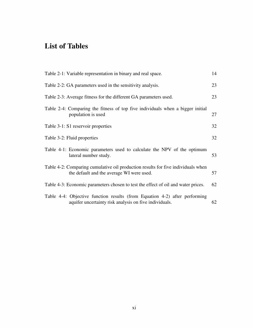
List of Tables
Table 2-1: Variable representation in binary and real space. 14
Table 2-2: GA parameters used in the sensitivity analysis. 23
Table 2-3: Average fitness for the different GA parameters used. 23
Table 2-4: Comparing the fitness of top five individuals when a bigger initial population is used 27
Table 3-1: S1 reservoir properties 32
Table 3-2: Fluid properties 32
Table 4-1: Economic parameters used to calculate the NPV of the optimum lateral number study. 53
Table 4-2: Comparing cumulative oil production results for five individuals when the default and the average WI were used. 57
Table 4-3: Economic parameters chosen to test the effect of oil and water prices. 62
Table 4-4: Objective function results (from Equation 4-2) after performing aquifer uncertainty risk analysis on five individuals. 62


xiii
List of Figures
Figure 1-1: Shaybah-220 well plan and design (picture courtesy of Saleri et al, 2003). 1
Figure 2-1: Reproduction procedure in GAs. 15
Figure 2-2: Crossover in bGAs. 16
Figure 2-3: Mutation in bGAs. 17
Figure 2-4: Flowchart of the overall optimization procedure using GAs. 18
Figure 2-5: Fittest individual performance comparison of three different runs and the average of the total six runs from the bGA and the cGA. 21
Figure 2-6: Moving average and percentage change of the objective function of the fittest individual as more runs are added in the bGA and cGA. 21
Figure 2-7: Fittest individual performance comparison averaged over three runs for different mutation probabilities. 24
Figure 2-8: Fittest individual performance comparison averaged over three runs for different mutation probabilities when a different initial population was used. 25
Figure 2-9: Population size for each generation in the three cases. The size is being held constant for the Base Case and dynamically assigned for Cases 1 and 2. 26
Figure 2-10: Fittest individual performance comparison averaged over three runs after using a constant population size for the Base Case and two designs for a dynamic population size in Cases 1 and 2. 27
Figure 2-11: Convergence of the fittest individual averaged over three runs for problems with different number of variables. 29
Figure 3-1: Average reservoir pressure and permeability maps for S1 reservoir. 33
Figure 3-2: Well parameter representation in the well optimization problem. 35
xiv
Figure 3-3: Oil and water relative permeability curves. 38
Figure 3-4: Implementing the indexing method on initial grid oil saturations. 38
Figure 3-5: Fittest individual performance comparison averaged over three runs with and without the saturation screening method. 40
Figure 3-6: Setting well vertical limits within the irregular grid geometry. 41
Figure 4-1: Fittest and average individual performance comparison averaged over three runs with different rejuvenation scenarios. Base Case: no rejuvenation applied. Case 1: rejuvenation applied to the whole population. Case 2: rejuvenation applied to half of the population. 48
Figure 4-2: The hill climber’s search pattern. 49
Figure 4-3: Flowchart of optimizing using genetic algorithms with the hill climber. 50
Figure 4-4: Fittest individual performance comparison averaged over three runs for different hill climber scenarios. Base Case: GA was run alone. Case 1: HC was run alone. Case 2: HC run at the end of GA. Case 3: Both algorithms run concurrently. 51
Figure 4-5: Percentage improvement in the objective function over previous generation with and without the HC 52
Figure 4-6: Cumulative oil production of the fittest individual averaged over three runs when using different number of laterals. 53
Figure 4-7: NPV of the fittest individual averaged over three runs when using different number of laterals. 54
Figure 4-8: Optimum well locations for: a) Deviated, b) Single-lateral, c) Dual-lateral, d) Tri-lateral, and e) Quad-lateral wells. 55
Figure 4-9: Comparing the trajectory of a well that returned high difference in cumulative oil production when the default and average WI were used. 57
Figure 4-10: Fittest individual NPV comparison averaged over three runs when running the optimization with default, weak, and strong aquifer strength values. 59
xv
Figure 4-11: Final well location and design for the weak, default, and strong aquifer strength values. 59
Figure 4-12: Cumulative oil production and water cut for the optimal solutions of the weak, default, and strong aquifer strength values 61
Figure 4-13: Individual performance comparison between the fine and upscaled model. 64
Figure 4-14: Objective function evolution of the fittest individual for the fine model. The initial population for this optimization composed from the fittest individuals from the upscaled model. 65
Figure 4-15: Comparison of well locations between: a) best individual in the fine model, b) Individual C from the coarse model (ranked 3rd in the coarse model but has similar locations to the individual in a), and c) best overall individual from the coarse model. 66

1
Chapter 1
1. Introduction
During the last two decades, horizontal wells have been used as the standard well type in
oil field development projects. More recently, technological advancements have
facilitated drilling of more complicated nonconventional well trajectories, which come in
variety of forms such as Multilateral Wells (MLWs) and Maximum Reservoir Contact
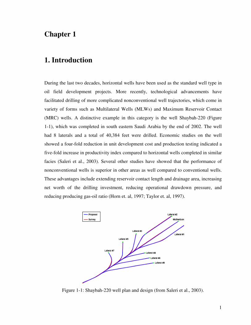
(MRC) wells. A distinctive example in this category is the well Shaybah-220 (Figure
1-1), which was completed in south eastern Saudi Arabia by the end of 2002. The well
had 8 laterals and a total of 40,384 feet were drilled. Economic studies on the well
showed a four-fold reduction in unit development cost and production testing indicated a
five-fold increase in productivity index compared to horizontal wells completed in similar
facies (Saleri et al., 2003). Several other studies have showed that the performance of
nonconventional wells is superior in other areas as well compared to conventional wells.
These advantages include extending reservoir contact length and drainage area, increasing
net worth of the drilling investment, reducing operational drawdown pressure, and
reducing producing gas-oil ratio (Horn et. al, 1997; Taylor et. al, 1997).
Figure 1-1: Shaybah-220 well plan and design (from Saleri et al., 2003).

2
However, the development of nonconventional wells poses several challenges. The real
oil fields are complex environments due to heterogeneities, presence of geologic
discontinuities (e.g. faults, fractures, and very high and low permeability zones), and
geologic uncertainties. Moreover, given the fact that MLWs require more initial cost than
conventional wells, the incremental value of the former might not be realized unless they
are optimally placed within the reservoir. Engineering intuition is not sufficient to
guarantee the optimum placement of these wells in most cases due to geological
complexity and nonlinear nature of the problem. Similarly, the usual industry practice of
trial and error to test multiple scenarios would rarely succeed to provide an optimum
solution in the multidimensional well placement optimization problem. As a result, there
is need for an optimization engine to evaluate the performance and viability of different
well placement scenarios and determine their optimum design.
The main objective of this work is to employ an efficient optimization technique to
identify a sound field development plan for a real field in Saudi Arabia. Optimized
parameters include well type (producer or injector), well placement, well and lateral
orientation, and number of laterals in each well. Further, we wish to investigate and
improve the available optimization procedures. For this purpose, a review of the
appropriate optimization procedures and an introduction of the problem are presented
next.
1.1. Literature Review
Copious and diverse research works relating to well placement optimization have been
discussed in the literature. While some studies focused on the placement problem, others
have explored applying proxies to speed the optimization process. In addition, other
studies tried to assess the performance of optimization under uncertainties. A survey of
the most relevant studies is presented next.
3
To begin this survey, we would like to shed some light on some work that applied general
optimization studies on well placement or design. Obi Isebor (2009) compared the
performance of several gradient-free methods like the Genetic Algorithm (GA), direct
search methods, and combinations of the two (GAs are explained in great detail in
Chapter 2. A subset of direct search methods, the hill climber, is described in Section
4.1.2). He used these algorithms to optimize control variables with multiple nonlinear
constraints on a channelized synthetic 2D model. He also applied penalty functions to
account for constraint violations. He concluded that, for problems considered, General
Pattern Search (GPS) with penalty functions perform the best followed by the combined
GA and GPS algorithm.
Handels et al. (2007) and Wang et al. (2007) proposed different approaches for well
placement optimization using gradient-based optimization techniques by representing the
objective function in a functional form. They then calculated the gradient of this function
and used a steepest ascent direction to guide the search. For the examples they
considered, these methods seemed promising due to their efficiency in terms of number
of simulation runs. The techniques were only applied to vertical wells and they expected
more difficulty in applying them to problems with arbitrary well trajectories in complex
model grids. Other issues they faced with these techniques include discontinuities in the
objective function and convergence to local optima.
The next couple of paragraphs will give special attention to work done with GA, which is
the optimization method used in this research. Bittencourt and Horne (1997) developed a
hybrid binary Genetic Algorithm (bGA), where they combined GAs with the polytope
method to benefit from the best features of each method. The polytope method searches
for the optimum solution by constructing a simplex with a number of vertices equal to
one more than the dimensionality of the search space. Each of the vertices is evaluated
and the method guides the search by reflecting the worst point around the centroid of the
remaining nodes. This work tried to optimize the placement of vertical or horizontal wells
in a real faulted reservoir. The algorithm sought to optimize three parameters for each
4
well: well location, well type (vertical or horizontal), and horizontal well orientation. The
study also integrated economic analysis and some practical design considerations in the
optimization algorithm.
Montes et al. (2001) optimized the placement of vertical wells using a GA without any
hybridization. They tried to discern the effects of internal GA parameters, such as
mutation probability, population size, initial seed, and the use of elitism. Their tests were
applied on two synthetic rectangular models (a layercake model and a highly
heterogeneous one). For the tested cases, they found that the ideal mutation rate should be
variable with generation. Using random seeds for their problem showed little sensitivity
while the use of elitism showed significant improvement. The population size study they
performed suggested that an appropriate size was equal to the number of the variables in
the problem. When they used very big populations, solution convergence was deterred as
more poor quality chromosomes had to be evaluated. They also drew attention to issues
like absolute convergence and stability of the optimization algorithm.
Emeric et al. (2009) implemented an optimization tool based on GA to optimize the
number, location, and trajectory of a number of deviated producer and injector wells.
They proposed a method to handled unfeasible solutions by creating a reference
population consisting only of fully feasible solutions. Any unfeasible solution
encountered in the optimization was repaired by applying crossover (refer to Section
2.3.1.1 for detailed description) between it and an individual from the reference
population until a new feasible solution was obtained. They applied this technique in
three full-field reservoir models based on real cases using two different strategies: the
first one with the whole initial population defined randomly; and the second one by
including an engineer’s proposal in the initial population. Better results were observed in
the second strategy and solutions were more intuitive for the tested case. They also
suggested and tested an alternative optimization approach by only optimizing well type
and number of an engineer’s proposal. Although final results were not as good as the full
5
optimization, they concluded that this approach can be used when there is time limitation
to perform the full optimization in complex cases.
Nogueira and Schiozer (2009) proposed a methodology to optimize the number and
placement of wells in a field through two optimization stages. The procedure started by
creating reservoir sub-regions equal to the maximum number of wells. Then, a search for
the optimum location of a single well was performed in each sector. The second stage
aimed to optimize well quantity through sequential exclusion of wells obtained from the
first stage. After a new optimum number of wells is reached, the first stage is performed
again until no improvement in the objective function is observed. This strategy showed
efficiency when tested on a heterogeneous synthetic model with light oil. They optimized
both vertical and horizontal wells in separate studies. They also concluded that the
proposed modularization of the problem speeds up the optimization process for their
problem of considertion.
Farshi (2008) converted a well placement and design optimization framework that was
developed by Yeten et al. (2002) from bGa to a real-valued continuous Genetic Algorithm
(cGA). A review of Yeten’s work is surveyed later in this section. He found that the cGA
provides better results when compared to the performance of bGA on the same synthetic
models. Moreover, he implemented several improvements to the optimization process
like imposing minimum distance between the wells and modeling curved wellbores.
Other studies sought to perform the task of well placement optimization under reservoir
geological uncertainty. Guyaguler et al. (2000) applied a hybrid optimization algorithm,
which also combines the features of bGAs with the polytope method. Furthermore, they
utilized several helper functions including Kriging and Artificial Neural Networks (ANN)
that act as proxies for the expensive reservoir simulations to reduce the optimization cost.
The theory of the Kriging algorithm is based on the phenomenon that some variables that
are spread out in space and time show a certain structure. The algorithm tries to
understand this structure and move towards the direction that is expected to achieve
6
desirable results. ANNs are nonlinear statistical data modeling tools that are designed
based on the aspects of biological neural networks. They seek to model complex
relationships between inputs and outputs or to find patterns in data after completion of a
training phase of the network that involves building a database from several simulation
runs. This study optimized the locations of several vertical injectors for a waterflood
project with the Net Present Value (NPV) as the objective function. Guyaguler et al.
concluded that Kriging was a better proxy than neural networks for tested problems. They
also conducted an uncertainty assessment study based on the decision theory framework.
An extensive sensitivity study was performed as part of their study to determine the effect
of the GA parameters.
Yeten et al. (2002) applied a bGA to optimize well type, location, and trajectory for
nonconventional wells. Along with that, they developed an optimization tool based on a
nonlinear conjugate gradient algorithm to optimize smart well controls. Several helper
functions were also implemented including ANN, the Hill Climber (HC). In addition,
they applied near wellbore upscaling, which approximately accounts for the effects of fine
scale heterogeneity on the flow that occurs in the near-well region by calculating a skin
factor for each well segment. The results of this study were presented on fluvial and
layered synthetic models, as well as a section model of a Saudi Arabian field. An
experimental design methodology was introduced to quantify the effects of uncertainty
during optimization. The study also conducted sensitivity analysis in a similar manner to
Guyaguler’s (2002) study.
Rigot (2003) extended the optimization engine developed by Yeten et al. (2002) by
implementing an iterative approach to improve the efficiency of multilateral well
placement optimization. He divided the original problem into several single well
optimizations to speed-up the optimization process and improves results. He also applied
a proxy to avoid running numerical simulation if the expected productivity of a certain
well was within the range of validity of the proxy.

7
Although previously commented studies provided promising optimization results, the
used techniques consumed long optimization time. It is commonly unfeasible and
computationally very expensive to conduct full optimization on some cases. To accelerate
the optimization process, other work concentrated in designing proxies to the reservoir
simulator. Pan and Horne (1998) used multivariate interpolation methods such as Least
Squares and Kriging as proxies to reservoir simulation. The purpose of the first algorithm
is to construct a function that has a simple known form to approximate some objective
function. The behavior of this objective function is first observed through a number of
simulations. Then, a function is constructed such that it minimizes the sum of the squared
residual between data and the function values. To begin their study, they selected several
well locations for numerical simulation as a sample to train the proxy. Then, Net Present
Value (NPV) surface maps were generated using the two proxies. These maps were
subsequently used to estimate objective function values at new points. They observed that
the Kriging method provides more accurate means to estimate the objective function than
the Least Squares interpolation in the tested examples.
Onwunalu (2006) applied a statistical proxy based on cluster analysis into the GA
optimization process for nonconventional wells. His work also used Yeten’s multilateral
well model. The objective of applying the proxy is to reduce the excessive computational
requirements when optimizing under geological uncertainty. The method is similar to the
ANN method in terms of building a database of simulation results. The data base is then
partitoned in clusters containing similar objects. The objective function of a new scenario
can be approximated by assigning it to one of the constructed clusters. Additionally, his
work extended the proxy to perform optimization of multiple nonconventional wells
opened at different times. When simple wells were optimized the proxy provided a close
match to the full optimization by simulation only 10% of the cases. This percentage
increased to 50% when multiple nonconventional wells were optimized.
Although these studies showed the viability of using different optimization algorithms in
field development problems, there is an apparent lack of real field applications. Some of

8
the algorithms were only tested on synthetic models and more testing is needed on real
full-field reservoir models with complex geologic structures. This study approached the
well placement and design optimization from this angle as we will elaborate in the next
section.
1.2. Problem Statement
As stated earlier, while a MLW has high initial cost, its return on investment is usually
higher than that of a conventional well. In this work, we try to optimize a field
development scenario of a number of producers and injectors in terms of well
configuration (number of laterals), and most importantly, the location of the mainbore
and each of the laterals. Optimizing well locations also includes finding parameters that
achieves the best performing well trajectory. These parameters include the length and
orientation of each well segment. This results in a high number of variables, and thus,
high problem complexity. A number of constraints are enforced to the potential wells to
make sure they are physically achievable solutions. Some of these constraints are simple
maximum and minimum bounds, while others are highly nonlinear and require careful
handling.
Generally speaking, optimization problems search for the set of variables that achieves a
maximum objective function according to the following equation:
Find xopt such that: F(xopt) ≥ F(x) for all x ∈ Ω
Subject to LB < Cn(x) < UB (1-1)
Here, x represents a vector containing problem parameters, Ω symbolizes the search
space domain, and Cn corresponds to the problem constraints defined by upper and lower
bounds. F stands for the objective function we are trying to optimize. For the well
placement problem, this objective function can consider economic implications of the
solution represented by the NPV of the project. However, since the field in question is
operated by a national oil company (Saudi Aramco), the cumulative oil production is
selected here as the objective function unless otherwise stated. OPEC countries are

9
restricted by certain quotas and optimizing recovery is usually their ultimate goal rather
than NPV.
As surveyed in the previous section, several optimization methods have been studied in
the literature for similar problems. It must be emphasized that our method of choice
should be capable of handling the complex nature of the problem, which in some cases
involves more than 100 decision variables. Furthermore, the lack of analytical solutions
in most cases and the nonlinearity and noncontinuity of oil field optimization problems
limits the utilization of standard gradient based optimization methods (Montes et al.,
2001). The complexity of the problem also implies that the objective function surface can
contain several local optima, so the exploration criterion of the selected method must
overcome converging towards such points. These reasons, along some others that are
discussed in detail in Section 2.1, favor the employment of stochastic search methods that
are typically successful in solving complex problems. GAs are one of the most common
algorithms that belong to this category and they were chosen to solve this problem
because they are easy to parallelize and hybridize. To our imperfect knowledge, the cGA
in particular has only been tested on synthetic models for nonconventional well placement
optimization and it is of interest to test its performance under real fields.
The objective of finding optimum well location and design was approached in this work
through four main stages. Firstly, the performance of two variants of GA, the bGA and
the cGA, was compared and a decision was made on the more robust algorithm for this
problem. Secondly, the different internal algorithm parameters were tuned such that they
consistently provide good results. This stage also included quantifying the contribution of
adding helper tools and hybrid techniques to the search for optimum solutions. Thirdly,
the tuned algorithm was applied to a full-field reservoir model based on a real case that
we wish to optimize well locations and design for. The final stage involved investigating
the reliability of the provided solutions by conducting uncertainty analysis and testing the
effects of some of the assumptions made during optimization.
10
The used code for optimizing multilateral well placement using the cGA was developed
by Farshi (2008). Since the original code was designed for synthetic models, it has been
modified to be compatible with any real field with complex geological setup and irregular
grid sizes as detailed in later chapters. It is important, however, to note that the main
contributions of the author are as indicated above. More enhancements were introduced to
the code, including the implementation of a HC function, rejuvenation, and the minimum
saturation screening. Results were generated for several examples that are presented in
Chapter 4. Furthermore, the dynamic attributes of the code were modified to better suit
the given field. In the descriptions that follow, the general approach and added
improvements are discussed together.
The report will proceed as follows. In Chapter 2, a description of the optimization
algorithm used in this study is detailed. Comparisons between bGA and cGA are made
and parameter sensitivities are presented. Next, Chapter 3 provides a description of the
reservoir model in question with the problem parameters and imposed constraints. It also
focuses on practical implementation issues that arise when linking the optimization
algorithm to the reservoir model. Then, Chapter 4 presents results obtained from the
different cases run on the model. Additionally, an evaluation of the benefits of helper
tools and of the uncertainties and assumptions in the optimization are discussed. Finally,
Chapter 5 summarizes the conclusions of this work and gives suggestions for future work.

11
Chapter 2
2. Main Optimization Engine
Before approaching the well optimization problem, a number of issues regarding the
optimization engine need to be addressed. We have previously rationalized the appeal of
applying GAs to such a problem. This chapter gives detailed description of the
advantages and methodology of the algorithm. Then, it presents a comparison of the two
GA types and a justification of choosing the cGA over the bGA through conducting a
number of runs using each variant. Finally, the chapter discusses results of a sensitivity
study on the internal search parameters of the algorithm. These parameters were
exhaustively analyzed in order to reach a base case configuration to be used for well
placement optimization problem in this field.
2.1. General Description of Genetic Algorithms
The GA is a stochastic and heuristic search technique based on theory of natural
evolution and selection. The basic idea revolves around survival of the fittest and
solutions are evolved through mating (information exchange) of the best performing
solutions. An occasional alternation of the fit solutions is allowed to occur to explore
other parts of the search space or to avoid entrapment into local optima (Mitchell, 1996).
Using GAs for the well placement optimization problem has been found to be ideal due to
the following reasons:
• The algorithm can be easily parallelized because each of the individuals can be
evaluated separately.
• The search for optimum is geared towards finding the global optimum rather than
local optima.
• They perform well in problems where the fitness function is complex, discontinuous,
noisy, changes over time, or has many local optima (Holland, 1992).
12
• The algorithm is capable of manipulating many parameters simultaneously.
• No gradients are required during the optimization process.
• Since the initial population is composed of multiple solutions rather than a single one,
we have the opportunity to explore more of the search space at each generation.
• The algorithm can be enhanced and hybridized with other techniques.
2.2. Common GA Vocabulary
It should come as no surprise that most of the basic terminology used in GAs is inherited
from Genetic Sciences. In the list below, the most common terms are explained (Yeten,
2003; Onwunalu, 2006).
• Individual: The set of parameters that defines a particular feasible solution within the
search space.
• Chromosome: The coded notation of an individual.
• Gene: The coded representation of a single property within a chromosome.
• Generation: The iteration stage that the optimization process has reached.
• Population: The collection of individuals within the generation.
• Fitness: An evaluation of the quality of the objective function value for an individual.
The fittest individual in a population would have the highest objective function value
when compared to other individual in the same population.
• Seed: The initial population fed to the optimizer.
• Selection: A GA operator through which a number of the fittest individuals are kept
in the next generation. This operator assures that every new generation is at least as
good as the previous one.
• Crossover: Another operator that provides the main mating mechanism by which
new chromosomes are created. The operator is designed such that an efficient
information exchange and inheritance is achieved between generations.
• Mating: A mechanism used to ensure new genetic material is occasionally introduced
to the chromosome. This operator also provides access to different areas of the search
space.

13
• Reproduction: The process of applying GA operators described above to the current
population or a portion of it in an attempt to evolve it into a better solution.
• Parents: Two fit individuals that are randomly selected to go through reproduction.
• Offsprings: Individuals that result after completion of the reproduction procedure.
2.3. Binary vs. Continuous GAs
Two GA types are utilized in optimization problems, the bGA and the cGA. In bGAs, the
optimization process embodies coding the value of each variable to its corresponding
binary value, applying GA operators to the chromosome, obtaining the resulting
offsprings and remapping them into the real space. On the contrary, cGAs use real-valued
numbers directly. In addition to the GA advantages mentioned above, cGAs in particular
are more appealing to use for this problem for the following reasons:
• The individual can assume any value in the search domain providing higher resolution
when compared to the discrete bGA.
• It is easier to enforce variable adherence to the limits of the problem in cGA.
• The variable coding/decoding process in bGAs introduces translation deficiencies that
can be prevented in cGA. A common problem is encountered when a desired
transition between two adjacent values results in altering many binary bits in certain
parameters. In other instances, the alteration of one bit can cause dramatic change in
the value of other properties (Deb and Agrawal, 1995).
The chromosome in each variant of GA is formed by concatenating the properties of the
solution. As an example, Equation (2-1) shows how the chromosome is represented in
each GA for an arbitrary well, whose properties are listed in Table 2-1. The gene of each
property has to accommodate the maximum value of that property, which explains the
zeros to the left of some binary genes.
Binary = [0101101000000 10111101101000 011010101 1101010010]
Continuous = [2880, 12136, 213.3, 850] (2-1)
14
Table 2-1: Variable representation in binary and real space.
Property Real
Value
Maximum Var.
Value
Required Binary Length
Binary Equivalent
x-coordinate 2880 15000 14 0101101000000
y-coordinate 12136 15000 14 10111101101000
Rotation angle 213.3 360 9 011010101
length 850 1000 10 1101010010
2.3.1. Reproduction Operators
GA reproduction operators are designed to improve the performance of current
individuals in the population. Three major operators are used in this algorithm, which are:
selection, crossover, and mutation. The overall reproduction procedure is illustrated in
Figure 2-1. In selection, the fittest member of each generation is carried to the next one
(also called elitist selection). Moreover, members of the current population are selected as
potential parents for individuals in the next generation according to a user-defined cut-off
value. A fitness-proportionate selection is applied for this study; in which fitter
individuals are more likely, but not certain, to be selected. The following rank weighting
formula was used to calculate the probability of selecting an individual as defined by
Farshi (2008):
( )
∑ =
−+=
selectN
i
r
r
select
n
i
nNp
1)(
1,
(2-2)
where Nselect is the lowest rank of an individual that can be selected as a potential parent,
n is the ranking of the current individual, and r is a ranking scale factor (≥ 1) that is
applied to give higher weight to fitter individuals. Individuals that have a rank lower than
Nselect will be discarded and not selected for further reproduction. The other two GA
operators are explained in more detail in the following sections.
15
Figure 2-1: Reproduction procedure in GAs.
2.3.1.1. Crossover
The crossover operator is intended to simulate the analogous recombination process that
occurs in genetic chromosomes during reproduction. Crossover has been described as the
key element that distinguishes GAs from other optimization methods. This is because it
achieves an efficient transfer of information between successful candidates. With
crossover, individuals have the opportunity to evolve by combining the strengths of both
parents. On the other hand, an individual does not communicate with others in the
population when there is no crossover. In other words, each individual is exploring the
search space in its immediate vicinity without reference to what other individuals might
have discovered (Koza et al., 1999).
In bGAs, the simplest form of crossover can be implemented by cutting the parents’
chromosomes at a random point and swapping the two resulting portions (Figure 2-2),
which is called single-point crossover. Other common forms of crossover include multi-
point crossover, in which several points of exchange are set; and uniform crossover,
where the offspring’s genome value can be taken from either parent with a 50/50
probability. Crossover is only performed on a certain percentage of the population
according to the crossover probability, Pxo.
16
Figure 2-2: Simple crossover in bGAs.
Using the aforementioned swapping technique in cGAs means that the properties of the
current generation would be carried on to the next generation without introducing any
new values, which does not achieve the desired diversity in the generation. Losing
diversity in the population makes it more uniform, consequently leading to premature
convergence to a suboptimal solution. This problem, however, can be reduced by utilizing
crossover with blending as defined by Radcliff (1991) using the following equation:
( ) FiMi
new
i PPP ββ −+⋅= 1 , 10 ≤≤ β , (2-3)
where Pinew is the ith variable in a new individual, and PMi and PFi are the property values
of the same variable from the mother and father individuals, respectively. β is a blending
coefficient that can remain constant for each crossover operation, or can be randomly
chosen for each single property. In this study, we opted for the latter approach because it
is more likely to diversify the population (Farshi, 2008). The limits of β bounds values of
the new property between that of the mother (β = 1) and that of the father (β = 0). Again,
the number of variables within an individual that will undergo the above process is
determined by Pxo.
2.3.1.2. Mutation
In contrast to crossover, which is responsible for the exploitation and evolution part of the
evolution process; mutation adds a randomness factor to the search process to allow the
solution to explore new areas of the search space. The main concept of mutation is to
cause small random alterations at single points in the chromosome. The number of

17
mutation occurrences is governed by the mutation probability, Pmut, which is usually
small (in the order of 0.01 to 0.1). Since any bit of a binary chromosome can only take
two values, mutation can be applied in bGAs by switching the value of bits that are
selected for mutation as shown in Figure 2-3.
Figure 2-3: Mutation in bGAs.
Although the implementation in cGAs is different, the main function of mutation remains
the same. Mutation in this algorithm can be attained by adding a normally distributed
random number to the variable selected for mutation as shown in Equation (2-4) (Haupt
and Haupt, 2004):
)1,0(NPPold
i
new
i ⋅+= σ , (2-4)
where Pold and Pnew are the property values before and after mutation, respectively. N is a
randomly distributed number between zero and one, and σ is the standard deviation of
this property in the current population. The added value is scaled by the standard
deviation of the current property to make sure the property does not exceed its feasible
range.
2.3.1.3. Overall Optimization Workflow
The reproduction procedure described above is just one part of the optimization loop.
Figure 2-4 shows a flow chart of the complete procedure. In a step-wise fashion, the main
GA optimization stages are:
1. Define optimization parameters and their limits.
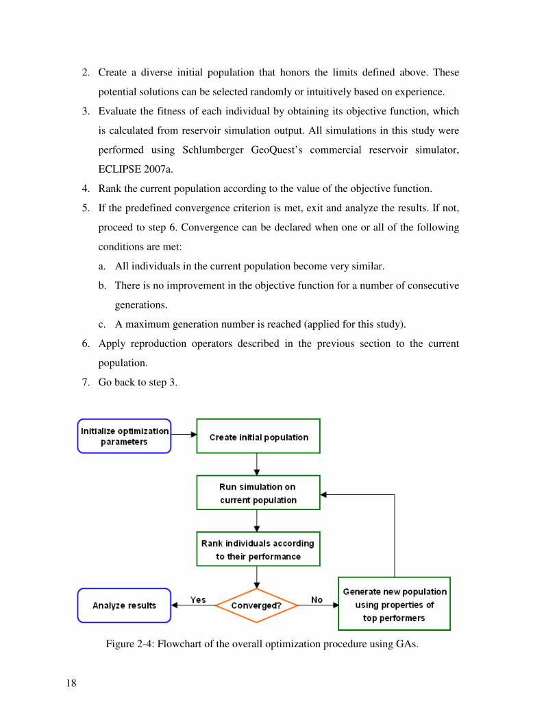
18
2. Create a diverse initial population that honors the limits defined above. These
potential solutions can be selected randomly or intuitively based on experience.
3. Evaluate the fitness of each individual by obtaining its objective function, which
is calculated from reservoir simulation output. All simulations in this study were
performed using Schlumberger GeoQuest’s commercial reservoir simulator,
ECLIPSE 2007a.
4. Rank the current population according to the value of the objective function.
5. If the predefined convergence criterion is met, exit and analyze the results. If not,
proceed to step 6. Convergence can be declared when one or all of the following
conditions are met:
a. All individuals in the current population become very similar.
b. There is no improvement in the objective function for a number of consecutive
generations.
c. A maximum generation number is reached (applied for this study).
6. Apply reproduction operators described in the previous section to the current
population.
7. Go back to step 3.
Figure 2-4: Flowchart of the overall optimization procedure using GAs.
19
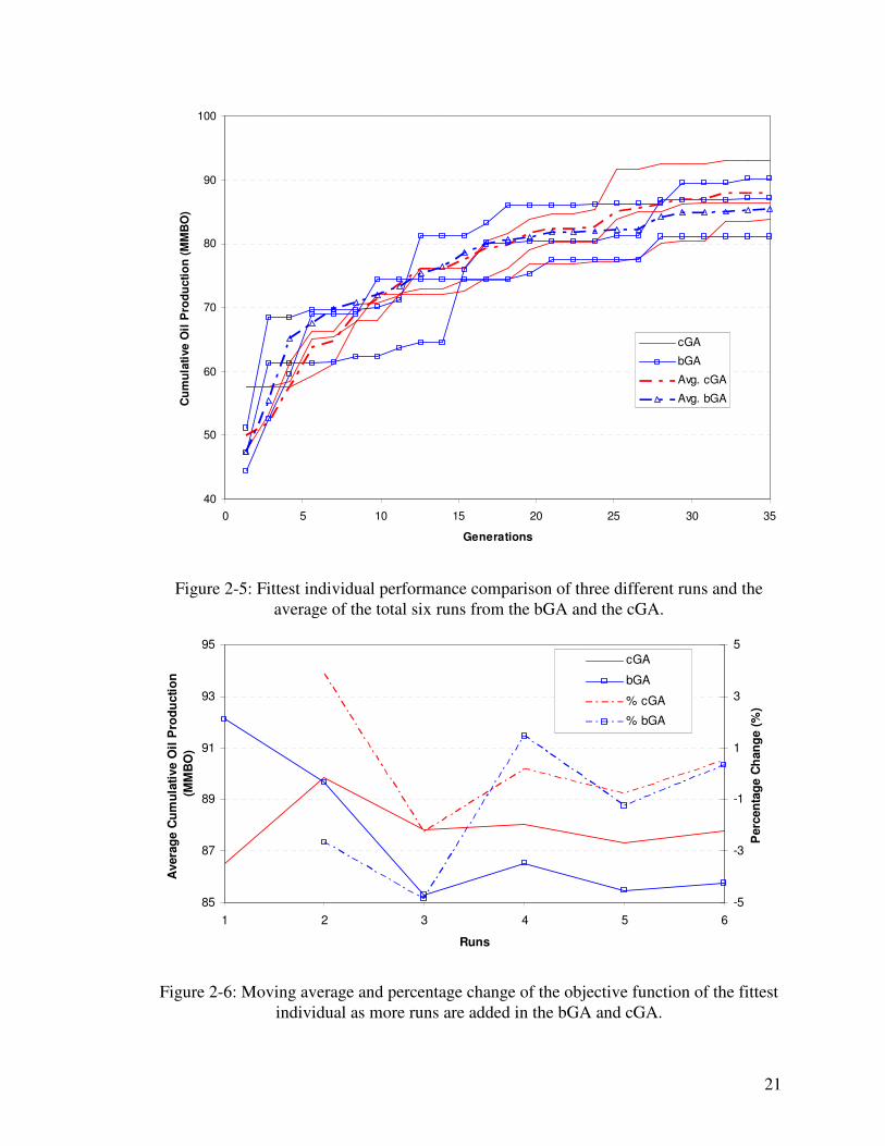
2.3.2. Performance Comparison
After understanding the mechanism of the two variants of GA, it is of interest to test
which of them is more suitable for this problem by comparing their performance. The
following exercise was designed to achieve this objective by finding the best location and
configuration for three deviated producers and two deviated injectors completed in the
reservoir described in Section 3.1. A population size of 30 was used, which is equal to the
number of variables. The optimization ran for 35 generations, which seems more than
sufficient for the size of this problem. A rationale of the choice of these numbers is
discussed in Sections 2.4.2 and 2.4.3. This results in 1050 simulations. Cumulative oil
production over a ten-year period is used as an objective function. All other GA and
optimization parameters were kept the same for the two GAs.
Binary coding of problem variables resulted in a chromosome length of 270 bits. To
provide more efficient crossover for this chromosome, the implemented bGA involves
using multi-point crossover with a total crossover points equal to the number of well
segments. Mutation had to be controlled for this exercise in order to make it only possible
for bits that do not produce invalid solutions. For instance, the chromosome of a wellbore
that has a z-coordinate of 4550 feet is represented in binary bits by 1000111000110. If the
limits in this coordinate were between 4470 and 4620 feet, mutating any of the first six
bits would generate invalid solutions. This kind of check was performed for all variables.
Both algorithms were run six times with a different random initial population for each
run. Figure 2-5 compares the evolution of the objective function for the best individual in
three of the runs for each method, as well as the averages of the six runs. A number of
observations can be made from this plot. First, the cGA evolves the solution in a gradual
fashion. Conversely, the bGA in general shows some jumps followed by flat regions.
Second, the average of the two methods is close until the end of the run, where cGA
shows slight advantage. Third, the individual runs in the cGA are more clustered around
20
its average than the bGA. This might give an indication about the robustness of the
algorithm; we are more likely to get a good answer with cGA if fewer runs are performed.
Another measure of robustness is provided by the repeatability of the algorithm. The
moving average for each algorithm was calculated by averaging objective function results
by the end of optimization after an additional run has been performed. As previously
mentioned, each algorithm was run six times. This means that the moving average by the
end of the third run, for example, is the mean of the objective function of the best
individual from these three runs when the run has ended. This average for cGA and bGA
is plotted in Figure 2-6 along with the percentage change in the average after an
additional run is added. The plot indicates that the average in cGA is stabilized after
around three runs. We consider the average to be stabilized if the change from adding an
additional run was within ±1% because it is unlikely that a decision would be changed
based on such a small change. In contrast, the bGA required five runs for its average to
reach the above stable region. In all subsequent runs, the cGA will be repeated three times
to obtain a more representative average.
Another advantage that gives more preference for the cGA is the lenience it provides in
handling the set of constraints and variables for the problem of interest. Some constraints
(particularly vertical well limits as we will see in Section 3.3.2) are difficult to capture
with the bGA. Since invalid reproduced solutions are handled by repeating the whole
reproduction procedure, the reproduction step in bGA consumes considerably more time.
On average, reproduction was completed in about 42 seconds per generation in bGA as
opposed to just 3 seconds in cGA, which increases the computational cost of
optimization. Other optimization steps were completed in around the same time for both
algorithms.
21
40
50
60
70
80
90
100
0 5 10 15 20 25 30 35
Generations
Cu
mu
lati
ve O
il P
rod
ucti
on
(M
MB
O)
cGA
bGA
Avg. cGA
Avg. bGA
Figure 2-5: Fittest individual performance comparison of three different runs and the
average of the total six runs from the bGA and the cGA.
85
87
89
91
93
95
1 2 3 4 5 6
Runs
Avera
ge C
um
ula
tive O
il P
rod
ucti
on
(MM
BO
)
-5
-3
-1
1
3
5
Perc
en
tag
e C
han
ge (
%)
cGA
bGA
% cGA
% bGA
Figure 2-6: Moving average and percentage change of the objective function of the fittest
individual as more runs are added in the bGA and cGA.
22
2.4. Sensitivity to cGA parameters
Due to the stochastic nature of GAs, the final solution of the same problem is usually
different when the algorithm is run a number of times. This is due to the different GA
probabilities, selection fractions, initial population, and number of generations. In this
section, the effects of each of these factors on the final solution given by the GA were
studied. A better understanding of the effect of each parameter might help us in
empowering the search process of the algorithm. Moreover, setting all parameters to their
best tested value would provide us with a starting ground to apply the algorithm on the
well placement optimization for this field.
2.4.1. Sensitivity to Operators’ Probabilities and Fractions
This test was performed to tune the effect of each GA operator. Several studies have
indicated that crossover and mutation probabilities have the most effect on the results
(Guyaguler, 2002; Yeten, 2003; Farshi, 2008). The selection fraction
( totalselectselect NNf = ) is also included in this study to account for the third GA operator,
selection.
The test was designed by selecting a low, a medium, and a high value for crossover and
mutation probabilities; and two values for the selection fraction. These values and all
other GA parameters used for this run are listed in Table 2-2. We ran the optimization by
varying one parameter at a time while fixing all other parameters. Note that the
population size and maximum generation value remain constant for this study. Separate
investigations for these two parameters are presented in the following two sections. Each
case is repeated three times to reduce the stochastic effect of the algorithm. Also, the
same initial population was used to eliminate the effect of initial population. This results
in 54 different runs. The objective function is the same to what was defined in the
previous example. The quality of each run was determined by averaging the objective
function value of the fittest individual from the three runs, which are listed in Table 2-3.

23
Table 2-2: GA parameters used in the sensitivity analysis.
GA Parameter Value
Population size 20
Maximum generation 30
Crossover probability [0.4, 0.6, 0.8]
Mutation probability [0.01, 0.05, 0.1]
Selection fraction [0.5, 0.8]
Ranking scale 2
Table 2-3: Average fitness for the different GA parameters used.
fselect = 0.8 fselect = 0.5
Pxo Pmut
0.4 0.6 0.8 0.4 0.6 0.8
0.01 53.9 54.2 53.1 50.7 53.8 56.1
0.05 52.6 56.6 66.1 54.3 59 63.2
0.1 49.2 56 56.2 51.5 57.9 61.6
In general, higher crossover probability and medium mutation probability achieved better
results. This is consistent with the conclusions of Yeten (2003) and Farshi (2008), where
the optimum Pxo values were found to be between 0.8 and 1.0 and optimum Pmut values
were in the neighborhood of 0.04 to 0.05. No firm conclusion could be drawn about the
effect of the selection fraction by looking at the average results. However, selecting half
of the population as potential parents seems to be more consistent.
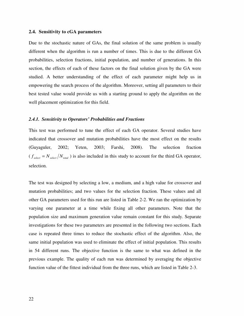
An interesting phenomenon was observed in the solution evolution of different Pmut
values plotted in Figure 2-7. While the performance of high Pmut (shown in green) is
clearly lower than the other two probability values, low Pmut (blue) appears to be better in
the early stages of the optimization than the medium value (red). This advantage is
reduced as we reach the later parts of optimization and low Pmut seems to cause premature
convergence as no improvement is observed in the last 15 generations. A similar study by
Montes et al. (2001) and Emerick et al. (2009) reached the same conclusion. They
24
suggested the need for low mutation rates in the beginning because allowing high rates at
this stage would overshadow the role of crossover. In later generations, however, a high
mutation rate is needed as solutions become more evolved and homogeneous. This high
mutation rate maintains diversity in the population, which increases the possibility of
finding optimum solutions. Results in Figure 2-7 are for Pxo = 0.8 and a selection fraction
of 0.5 but most other combinations showed similar trends.
20
30
40
50
60
70
0 5 10 15 20 25 30
Generations
Cu
mu
lati
ve
Oil
Pro
du
cti
on
(M
MB
O)
Pmut = 0.01
Pmut = 0.05
Pmut = 0.1
Dynamic Pmut
Figure 2-7: Fittest individual performance comparison averaged over three runs for
different mutation probabilities.
To exhibit the advantages of medium and low mutation probabilities, an additional run
was made with a dynamic mutation probability. The orange curve shows the result for
this run where Pmut was set to 0.01 until the end of the tenth generation, then increased to
0.05 thereafter. This change shows an improvement of approximately 8% over Pmut =
0.05. To confirm the above results, the same procedure was repeated with a different
initial population, results of which are plotted in Figure 2-8. The benefits of
implementing dynamic mutation are even more apparent in this example. Nonetheless,
the point at which the low mutation probability stops evolving the solution is different
here (after around 14 generations compared to 10 in the previous example). This makes it

25
interesting to change the mutation probability automatically when the low value stops
improving the solution after a consecutive number of generations instead of using a fixed
generation as implemented here. This improvement, however, was not implemented due
to time limitations.
30
40
50
60
70
80
0 5 10 15 20 25 30
Generations
Cu
mu
lati
ve O
il P
rod
ucti
on
(M
MB
O)
Pmut = 0.01
Pmut = 0.05
Pmut = 0.1
Dynamic Pmut
Figure 2-8: Fittest individual performance comparison averaged over three runs for
different mutation probabilities when a different initial population was used.
2.4.2. Sensitivity to Initial Population
As previously discussed, GAs are seed dependent algorithms. Fitter initial populations are
more likely to produce better solutions. The population size depends on the nature,
complexity, and number of variables of the problem. Typically, the population is
generated randomly such that it covers the entire range of possible solutions. A couple of
studies have suggested that problems of moderate complexity problems should have a
population size equal to the chromosome’s bitstring length in bGA (Goldberg, 1989;
Alander, 1992; Montes, 2001). An analogous population size for cGAs has not been
established in the literature; hence, a simple test was designed to investigate the issue.
Traditionally, the rule of thumb is to make the population size equal the number of
variables in the problem, which we based the Base Case design on. Two more cases were

26
run. Case 1 had an initial population size that is double the number of variables. All
individuals in this initial population are evaluated but the optimization proceeded with
only the better half. Case 2 had the same initial population as in Case 1 but the population
is reduced dynamically as the optimization progresses. The population size of each case is
schematically explained in Figure 2-9. The run and well specifications are similar to those
defined in the previous section with Pmut = 0.01 changing to 0.05 after the tenth
generation, Pxo = 0.8, and fselect = 0.5.
Figure 2-9: Population size for each generation in the three cases. The size is being held
constant for the Base Case and dynamically assigned for Cases 1 and 2.
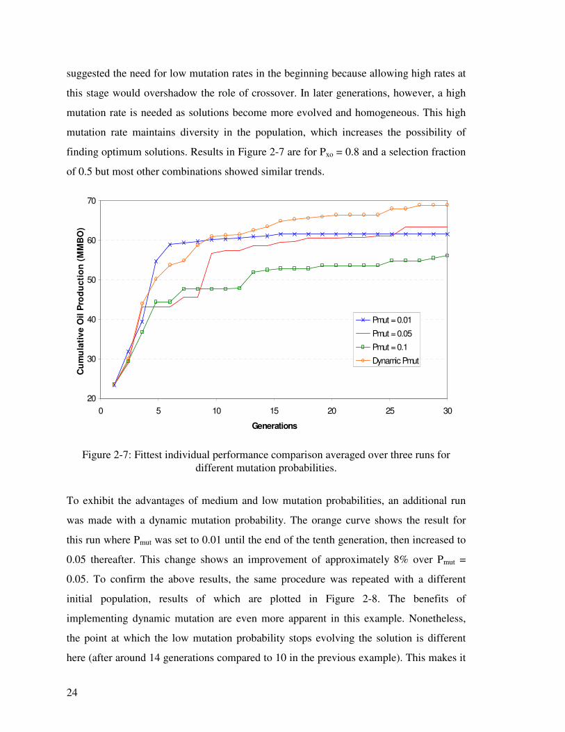
Each case was repeated three times and average results of the fittest individual are plotted
in Figure 2-10. Case 1 showed improvement over the Base Case only at the beginning of
optimization. The reasoning behind this occurrence becomes clearer after looking at the
objective function of the top five individuals from each case listed in Table 2-4. Because
of the larger initial population for Case 1, fitter individuals were introduced, which
translated to better solutions in the beginning of the run. However, the algorithm in the
Base Case was eventually able to evolve and reach similar objective function values to
those returned by Case 1 by the end of the run. Case 2, on the other hand, performs better
from the beginning and maintains the advantage until the end of the run. The difference
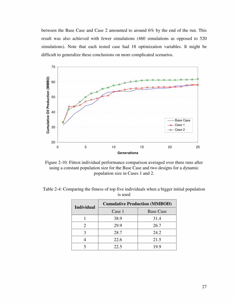
27
between the Base Case and Case 2 amounted to around 6% by the end of the run. This
result was also achieved with fewer simulations (460 simulations as opposed to 520
simulations). Note that each tested case had 18 optimization variables. It might be
difficult to generalize these conclusions on more complicated scenarios.
20
30
40
50
60
70
0 5 10 15 20 25
Generations
Cu
mu
lati
ve
Oil
Pro
du
cti
on
(M
MB
O)
Base Case
Case 1
Case 2
Figure 2-10: Fittest individual performance comparison averaged over three runs after
using a constant population size for the Base Case and two designs for a dynamic
population size in Cases 1 and 2.
Table 2-4: Comparing the fitness of top five individuals when a bigger initial population
is used
Cumulative Production (MMBOD) Individual
Case 1 Base Case
1 38.9 31.4
2 29.9 26.7
3 28.7 24.2
4 22.6 21.5
5 22.5 19.9

28
2.4.3. Required Number of Generations
An important question that we must answer before applying this algorithm to a real field
is how long the optimization should run. Without consideration to urgencies that might
come up in a real scenario, the interest here is to find out how many generations are
required for a certain optimization to converge. This, of course, is also dependent on the
complexity of the problem represented by the number of variables. To discern the effect
of number of variables on the maximum required generation, three cases were optimized
for 60 generations. The three cases were picked to represent a relatively simple, a
moderately complicated, and a complex problem. The first case contains three deviated
producers and two deviated injectors. The second and third cases consist of the same
number of wells but each well has two and four laterals, respectively. The resulting
number of variables (from Equation 3-3 to be discussed in Chapter 3) for this set-up is 30,
70, and 110 for the three cases. Each case was repeated three times and the average
results of the fittest individual are plotted in Figure 2-11. Note that the objective from this
exercise is not to compare the performance of the three cases but rather to select an
appropriate maximum number of generations for each case. Assuming that convergence
have occurred when no improvement in the objective function has taken place for ten
consecutive generations, it appears that 25 generations are sufficient to provide a
converged solution when 30 variables are used for the analyzed case. This number
increased to around 32 when the number of variables was increased to 70. When 110
variables were used, 45 generations were required to reach a converged solution.

29
30
60
90
120
150
0 10 20 30 40 50 60
Generations
Cu
mu
lati
ve O
il P
rod
uc
tio
n (
MM
BO
)
30 Variables
70 Variables
110 Variables
Figure 2-11: Convergence of the fittest individual averaged over three runs for problems
with different number of variables.
2.5. Concluding Remarks
In this chapter, we have justified the suitability of using GAs in high dimensional
optimization problems such as well placement and design optimization. We have further
shown that the cGA yields better results than the bGA for this particular field, and
therefore, it was used as the main optimization algorithm. Sensitivity analysis was
performed to determine the best combination of internal cGA parameters. This analysis
showed that dynamic mutation, 0.8 crossover probability, and 0.5 selection fraction
returned the best results. A dynamic population size also showed an improvement in
results with less number of simulations. For the tested case, it was found that running
the optimization for three times attained a representative average of the objective
function. Finally, the number of needed generations depends on the complexity of the
problem. 25, 32, and 45 generations were needed to get a converged solution when 30,
70, and 110 variables were used, respectively.

30
Having decided on an optimization algorithm to be used for this problem, the next
chapter will describe the needed steps to smoothly apply this algorithm to the reservoir
model at hand.

31
Chapter 3
3. Practical Framework of Well Placement
Optimization
Within the optimization process, numerous interactions take place between the GA and
the reservoir simulator. The two parts have to be completely compatible in order to have a
trouble-free process and reliable solutions. The purpose of this chapter is to establish a
good understanding of the reservoir model and the optimized parameters. Such an
understanding will ease integration between the two parts. This chapter also describes
how to ensure that invalid solutions are prevented by adhering to the problem’s
constraints. Implementation of some of the important nonlinear constraints is
demonstrated along with the resulting optimization improvements from this step. Lastly,
some of the important interaction steps between the optimizer and the reservoir model,
such as the information exchange mechanism and objective function calculation, are
briefly explained.
3.1. Reservoir Model Description
The model is for a carbonate reservoir in offshore Saudi Arabia. In all subsequent text,
this reservoir will be referred to as the S1 reservoir. The reservoir extends over a 26 by 41
km area and is currently under evaluation for full development. As can be seen in Figure
3-1, oil has accumulated due to a dome stratigraphic trap. Although only 14 vertical
observation wells have been completed in S1, many wells were drilled to a deeper
reservoir in the same field. Therefore, many core samples and open hole log data are
available for S1 reservoir. From these data, it has been recognized that permeability is
mildly heterogeneous (Figure 3-1). While most areas have a permeability of around 200
mD, high permeability (1-2 Darcy) areas are scattered around the field. An areally
isotropic permeability is used in the model with a vertical to horizontal permeability ratio

32
of 0.05. Other important reservoir, rock, and fluid properties are listed in Table 3-1 and 3-
2. Because the field is operated above the bubble point pressure, the simulation model
only contains the oil and water phases.
Table 3-1: S1 reservoir properties
OOIP 2.4 BSTB
Φ* 23%
k* 300 md
kz / kh 0.05
Average gross thickness 151'
T* 145 ˚F
P*res 1738 psig
cr* 4.5x10⁻⁶ psi-1
* for average
Table 3-2: Fluid properties
Pbuble 876 psia
Solution GOR 224 scf / STB
Crude Grade 28.9 API
µo 4.8 cp
Bo 1.13 BBL / STB
co 6.5x10⁻⁶ psi-1
λw 1.16
µw 0.52 cp
Bw 1.00 BBL / STB
cw 3.00x10⁻⁶ psi-1

33
Figure 3-1: Average reservoir pressure and permeability maps for S1 reservoir.
The reservoir model constructed by Saudi Aramco is 69 x 122 x 14 (117,852 total cells).
A structured grid is used and cell dimensions vary in each direction, which contributes to
the geometrical complexity. Since the optimization process involves thousands of
simulations, an upscaled version of the model was obtained. The fine model was
coarsened with a ratio of 3:1 in each of the two areal directions while keeping the vertical
resolution to contain the thin shale layers existing in the reservoir. The resulting coarse
model dimensions are 23 x 41 x 14 (13,202 total cells). Simulations on the upscaled
model were faster than those on the fine model by approximately a factor of 40. Hence,
this model was used to obtain all results to be presented in Chapter 4, unless otherwise
specified. In Section 4.5, a final optimization run on the fine model is discussed and the
results are compared with the coarse model.
3.2. Problem Variables
The optimized variables in this problem were chosen such that they possess three
important characteristics. Firstly, they have to be independent because each variable is
selected and mated randomly with other individuals. Choosing independent variables also
allows us to work with the lowest possible set of variables for the problem. Reducing the
number of variables would help to reduce the complexity of the problem and ease the

34
optimization process. Secondly, the variables should have significant physical meaning
such that there is a strong connection between them and the objective function values. By
doing so, GA operators are more capable of directing the search towards the optimum
solution during the information exchange process. Finally, the variables should be easy to
handle during the constraint enforcement stage. More elaboration on this issue will follow
in the next section.
In this work, we use the variable set defined by Farshi (2008). Since the well’s mainbore
can be represented by a straight line in the 3D space, six variables are sufficient to define
its trajectory. These variables are: the three coordinates of the midpoint (xmid, ymid, zmid),
total well length (Ltot), vertical well distance between the tow and the heel (Zh), and the
top-view rotation angle (Ө). Using Zh as a variable is very handy in creating wells within
the vertical limits of the reservoir. When it comes to laterals, four variables would
completely define their orientation since one degree of freedom is lost as they are fixed to
the mainbore. As a consequence, defining one variable (junction position relative to the
total mainbore length, Jp) can replace the three midpoint coordinates. The other two
lengths and angle variables complete the lateral’s definition. Figure 3-2 provides a
visualization of the variable set. Other dependent parameters that are needed during
optimization, such as heel and toe coordinates of the mainbore and laterals, can be
calculated from the independent variables stated above according to the following
equations:
well
h
well
mid
well
toeheel
wellwell
xy
well
mid
well
toeheel
wellwell
xy
well
mid
well
toeheel
Zzz
Lyy
Lxx
2
1
cos2
1
sin2
1
,
,
,
±=
±=
±=
θ
θ
( )( )( )
22
htotxy
well
heel
well
toep
well
heel
lat
heel
well
heel
well
toep
well
heel
lat
heel
well
heel
well
toep
well
heel
lat
heel
ZLL
zzJzz
yyJyy
xxJxx
−=
−+=
−+=
−+=
(3-1)

35
Figure 3-2: Well parameter representation in the well optimization problem.
With the optimization variables in place, a chromosome can be constructed by
concatenating the producers’ properties until the total number of producers is reached
(Pnum), followed by the injectors’ properties until we reach total number of injectors
(Inum). The chromosome is eventually represented as a vector containing all parameters to
be optimized as shown in following equation:
Chromosome = …,prod(n), … , prod(Pnum), …, inj(m), … , inj(Inum)
prod(n) = ),....],,,(),...,,,,,,[( )()()()( ilatilat
h
ilat
tot
ilat
p
mbmb
h
mb
tot
mb
mid
mb
mid
mb
mid ZLJZLzyx θθ
inj(m) = ),....],,,(),...,,,,,,[( )()()()( jlatjlat
h
jlat
tot
jlat
p
mbmb
h
mb
tot
mb
mid
mb
mid
mb
mid ZLJZLzyx θθ
(3-2)
As we are basing the population size on the number of variables, it is very important to
use a low number of variables at any optimization. This number is proportional to the
number of wells and laterals in each well as demonstrated by Equation (3-3). Increasing
the number of wells and laterals can substantially increase optimization time and
complexity.
( )( )countcountcount LatWellVar 46 += , (3-3)
Varcount above is the total number of decision variables in the problem, Wellcount is the
total number of wells, and Latcount is the number of laterals in each well. A description of
the procedure of creating new individuals using this set of variables is presented next.
36
3.3. Constructing the Initial Population
Creating an individual that contains a number of wells with the desired variables is not a
trivial task. As the model being used for optimization is for a real field, we had to make
sure all proposed solutions are feasible. This means that they must be within the physical
constraints for that particular field. Several constraints have been enforced on the initial
population. Some of these constraints were imposed to make sure the resulting wells are
drillable, while others are put in place to avoid creating solutions that are known to
perform poorly due to violating common engineering practices. Considering that we have
control in the initialization process, the constraints can be easily applied to the initial
population. Nevertheless, reproduction might result in invalid solutions that we are
continually filtering and excluding from evaluation. Some of the simpler constraints are:
• The minimum distance between any well and all other wells/segments must be more
than 750’ to mitigate well interference effects. This number was recommended by the
reservoir management team for this field as it approximates the wells’ drainage area.
• The maximum total length of each lateral cannot exceed 4000’ to avoid swelling of
shale layers. These layers in this field are known to swell if exposed to drilling fluids
for long periods.
• The maximum possible Zh is set to 120’ since the average net pay in the reservoir is
150’.
• To avoid lateral emanation from the end of the mainbore, angle difference between
the two must be more than 30˚. This angle, however, should not exceed 90˚ as obtuse
angles between the lateral and mainbore are difficult to drill.
Considering an arbitrary property, P, initial properties relating to the last three constraints
can be generated by the following equation:
( )minmaxmin )1,0( PPrandPPinit −+= (3-4)
Other more complicated constraints will be explained in separate sections that will
follow.

37
3.3.1. Saturation Screening
During the early stages of this study, it was noticed that many individuals in the initial
population produce minuscule amounts of oil. These individuals impaired the quality of
the initial population and deterred the evolution process. Analyzing these individuals
revealed that most of them were completed in very low oil saturation (So) zones. This
motivated us to screen for grid saturations that candidate individuals should reside in. The
screening process can be considered as a rule-based constraint to avoid creating and
simulating potentially known poor performers.
Inspecting the relative permeability curves in Figure 3-3 shows that the residual oil
saturation (Sor) is around 0.4. Yet, the initial oil saturation in 39% of the cells is below
this relatively high Sor value. An indexing system similar to the one developed by
Bittencourt and Horne (1997) was applied to overcome this issue, where cells that do not
contain moveable oil will be excluded from the well location initialization process. An
example of this procedure is illustrated in Figure 3-4 for layer 4 (arbitrarily chosen) of the
reservoir model. Green areas correspond to cells with an initial So higher than Sor,
whereas red cells represent the other possibility.

38
0
0.2
0.4
0.6
0.8
1
0 0.2 0.4 0.6 0.8 1
Water Saturation
Re
lati
ve
Pe
rme
ab
ilit
y
Kro
Krw
Figure 3-3: Oil and water relative permeability curves.
5
10
15
20
25
30
35
40
5 10 15 20
5
10
15
20
25
30
35
40
5 10 15 20
Afterindexing
5
10
15
20
25
30
35
40
5 10 15 20
5
10
15
20
25
30
35
40
5 10 15 20
Afterindexing
Figure 3-4: Implementing the indexing method on initial grid oil saturations.
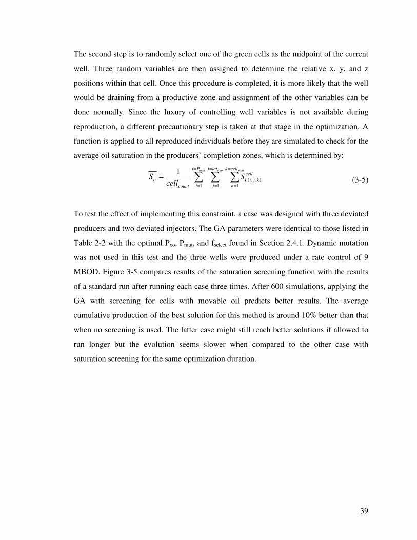
39
The second step is to randomly select one of the green cells as the midpoint of the current
well. Three random variables are then assigned to determine the relative x, y, and z
positions within that cell. Once this procedure is completed, it is more likely that the well
would be draining from a productive zone and assignment of the other variables can be
done normally. Since the luxury of controlling well variables is not available during
reproduction, a different precautionary step is taken at that stage in the optimization. A
function is applied to all reproduced individuals before they are simulated to check for the
average oil saturation in the producers’ completion zones, which is determined by:
∑ ∑ ∑=
=
=
=
=
=
=num num numPi
i
latj
j
cellk
k
cell
kjio
count
o Scell
S1 1 1
),,(
1 (3-5)
To test the effect of implementing this constraint, a case was designed with three deviated
producers and two deviated injectors. The GA parameters were identical to those listed in
Table 2-2 with the optimal Pxo, Pmut, and fselect found in Section 2.4.1. Dynamic mutation
was not used in this test and the three wells were produced under a rate control of 9
MBOD. Figure 3-5 compares results of the saturation screening function with the results
of a standard run after running each case three times. After 600 simulations, applying the
GA with screening for cells with movable oil predicts better results. The average
cumulative production of the best solution for this method is around 10% better than that
when no screening is used. The latter case might still reach better solutions if allowed to
run longer but the evolution seems slower when compared to the other case with
saturation screening for the same optimization duration.
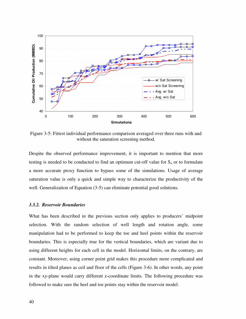
40
40
50
60
70
80
90
100
0 100 200 300 400 500 600
Simulations
Cu
mu
lati
ve O
il P
rod
ucti
on
(M
MB
O)
w/ Sat Screening
w/o Sat Screening
Avg. w/ Sat
Avg. w/o Sat
Figure 3-5: Fittest individual performance comparison averaged over three runs with and
without the saturation screening method.
Despite the observed performance improvement, it is important to mention that more
testing is needed to be conducted to find an optimum cut-off value for So or to formulate
a more accurate proxy function to bypass some of the simulations. Usage of average
saturation value is only a quick and simple way to characterize the productivity of the
well. Generalization of Equation (3-5) can eliminate potential good solutions.
3.3.2. Reservoir Boundaries
What has been described in the previous section only applies to producers’ midpoint
selection. With the random selection of well length and rotation angle, some
manipulation had to be performed to keep the toe and heel points within the reservoir
boundaries. This is especially true for the vertical boundaries, which are variant due to
using different heights for each cell in the model. Horizontal limits, on the contrary, are
constant. Moreover, using corner point grid makes this procedure more complicated and
results in tilted planes as ceil and floor of the cells (Figure 3-6). In other words, any point
in the xy-plane would carry different z-coordinate limits. The following procedure was
followed to make sure the heel and toe points stay within the reservoir model.

41
• Once the three midpoint coordinates, well length, and the rotation angle are
determined, calculate the x and y coordinates of the heel and toe.
• Devise plane formulas for the uppermost and lowermost planes bounding the (x, y)
point calculated above according to the following equations (Wikipedia, 2009):
0=+++ dznynxn planezplaneyplanex
pnd ⋅−= , (3-6)
where nx, ny, and nz are the three components of an arbitrary vector, n, which is
normal to the plane. p represents the coordinates of any point that belongs to the
plane.
• Use these formulas to find maximum and minimum possible z-coordinates for the
heel and toe.
• Set new limits for the variables Zh honoring zmin and zmax from above.
• Randomly choose a Zh value for the well between its limits.
Figure 3-6: Setting well vertical limits within the irregular grid geometry.

42
3.4. Preparing Input Files for the Reservoir Simulator and Reading Output Files
Once we are confident that all the individuals adhere to the constraints and can be passed
to the simulator, simulation input files are written for each individual. When a particular
scenario is being optimized, all reservoir model data are being held constant except for
the well data, which change from an individual to another. These well data have to be put
in a format that is readable by ECLIPSE. A MATLAB function was prepared to convert
well coordinates into the corresponding I, J, and K cell parameters. From these data, the
function prepares an include file containing all well design parameters specified by the
WELSPECS, COMPDAT, WCONPROD, and WCONINJ keywords in ECLIPSE. When
the simulation is finished, another function will read the resulting *.RSM file to obtain
production and injection data, from which an objective function is evaluated. Based on
this objective function a ranking of the individuals takes place and the optimization
continues.
3.5. Objective Function Definition
One of the input parameters that the user has to define prior to submitting an optimization
run is the type of objective function to be optimized. Two types are available in the
formulation of this work: cumulative production and NPV. After each individual is
simulated, calculation of each objective function is possible by reading the simulation
output file. While cumulative oil production represents a single value, the total oil volume
by the end of simulation; NPV takes more consideration of the economics of the project.
The economic model we used is based on the work of Yeten (2003). NPV is calculated
based on a fixed yearly effective discount rate as:
( ) d
Y
n wgop
p
n
pnCCQ
iNPV −
⋅
+= ∑ ∑
= =1 ,, 1
1 , (3-7)
where Qpn is the production rate of phase p during the year n, Cp is the unit profit or cost
associated with this phase, and i is the annual percentage rate (APR), Y is the total
number of discount years, and Cd is drilling and completion cost. Cd consists of several
costs associated with the drilling operation and is given by:

43
( )∑=
⋅++=countWell
i
millcountdrillitotCAPEXd CLatCLCC1
, , (3-8)
where CCAPEX is a capital expenditure cost per well including platform cost and the cost
of drilling to the top of the reservoir, Cdrill is the unit drilling cost per feet, Cmill is the cost
of milling a new junction, and the rest of the variables are as defined previously.
3.6. Other Implementation Issues
As a consequence of converting well coordinates from their real values to the
corresponding simulator I, J, and K values, completions are assumed to be at the center of
the grid blocks. As a result, straight well trajectories previously defined by the GA will be
represented in a staircase manner when converted to the grid space. The error introduced
by this phenomenon can be corrected by using the correct well index (WI) (Yeten, 2003).
Due to the complex grid geometry in this model, a computation of the accurate WI could
not be directly integrated into the optimization procedure and the default WI values given
by ECLIPSE were used. The effects of overlooking this correction will be discussed in
Section 4.4. Also, when the input well files were prepared for the simulator, it was
assumed that all well segments are fully perforated. Selective perforation can be used by
introducing new variables but it was not considered in this study.
Additionally, the technique for generation of the initial population can be improved. With
inaccessibility to openhole logs and other field data, all individuals in this study were
generated randomly. As more data become available, a well engineered initial solution
can be constructed and fed to the GA for improvement, which should generate better final
solutions (Emerick et al., 2009).
3.7. Concluding Remarks
In this chapter, a description of the reservoir model, problem parameters, and problem
constraints were presented. It was shown that applying some constraints that eliminate
expected poor performers, such as initial oil saturation screening, considerably improved
optimization results. A methodology for keeping the wells within reservoir limits via

44
planar geometry was also explained. Finally, this chapter detailed some of the important
interaction steps between the optimizer and the reservoir model, such as the information
exchange mechanism and objective function calculation.
Now that the overall optimization procedure is defined, we are ready to present the results
of applying it to the S1 reservoir model in the next chapter.

45
Chapter 4
4. Results and Discussion
After making a decision about the optimization algorithm and determining a reliable set
of GA parameters in Chapter 2, we are now ready to proceed to the third stage of the
study by applying the algorithm to the S1 reservoir model. The first step in this stage is to
investigate the possibility of further empowerment of the algorithm by combining it with
some helper tools. The resulting hybridized algorithm from this step was then run on the
field to draw some conclusions on the optimal field development plan. The final step was
to examine the reliability of obtained optimum solutions under different assumptions that
were made prior to the optimization. It is of high interest to find out if these solutions
remain superior had the assumptions not been made. This step involves an uncertainty
propagation study on the effects of aquifer strength, an assessment of assuming a default
WI for the wells, and an appraisal of any consequences caused by upscaling the original
reservoir model.
Unless otherwise mentioned, the following optimization parameters were used in this
chapter. All tests were performed with the GA parameters listed in Table 2-2 with Pxo =
0.8, Pmut dynamically assigned, and fselect = 0.5. Additionally, all producers were
simulated with a bottom-hole pressure (BHP) control of 1000 psig, which is above Pbub.
Injectors were operated with a BHP of 2500 psig. The population size of each run was
equal to the number of variables, which is calculated from Equation (3-3). The maximum
generation was adjusted appropriately to accommodate the complexity of the problem
according to the findings of section 2.4.3. Three runs were made to get a dependable
average of the studied case. In few cases, one of the three runs was omitted due to
abnormally low objective function value and a replacement run was performed.
Depending on the considered study and the expected economic implications, the objective
46
function was alternated between cumulative oil production and the NPV of the project.
The runs in this study were parallelized over 20 computer nodes.
4.1. Helper Tools
One of the advantages of the GA mentioned earlier is the ability to hybridize them with
different optimizers and helper tools. Some of these helper tools are designed to speed up
the algorithm, while others focus on improving the final GA solutions. Some of the most
commonly used tools in the literature are ANNs, the Hill Climber, and Rejuvenation. The
first helper tool was not implemented as Rigot (2003) has found that the method requires
substantial simulation time to train ANN in order to see plausible improvement in
complex reservoir models. The other two functions were already tested by Yeten (2003)
on a synthetic model and are duplicated in this work to find out how well the algorithm
performs in real field applications. Results of their implementation are presented next.
4.1.1. Rejuvenation
The basic concept of rejuvenation is quite simple; the best solutions encountered during
the overall optimization are resurrected during some specified generation levels. Because
these solutions might have belonged to generations older than the previous generations,
they will be referred to as ancestors (Fichter, 2000). These ancestors might have been
mutated in an unfavorable manner and bringing them back creates opportunities for better
mating of the top individuals, and thus, better offspring.
Rejuvenation was tested by optimizing the location of three producers and two injectors,
each having three laterals. It was applied by keeping a pool of a similar size to the
population. This pool keeps track of the fittest individuals during the course of
optimization and composes the new population every five generations. Mutation is still
applied to all individuals except the fittest one, but no crossover is considered during this
generation. This optimization case will be referred to as Case 1, whereas the Base Case
was run normally without rejuvenation. Each case was run for three times and the average
results are plotted in Figure 4-1. When comparing the outcome of the Base Case (blue

47
curve) with Case 1 (red curve), it can be concluded that rejuvenation did not introduce
noticeable improvement to the objective function of the fittest individual. An explanation
of this finding might be realized when looking at average objective function of all
individuals within the generation shown in dashed lines of the same colors. Jumps in the
average values are introduced by rejuvenation every five generations. These jumps are
sometimes high enough to bring the average fitness of individuals within a population to
a very close value of the fitness of the best individual in this population. This is an
indication of the similarity and loss of diversity in the different solutions in the
population, which weakens the evolution process of the GA.
Case 2 was designed to alleviate the aforesaid drawback of losing population diversity.
Instead of composing the whole population by rejuvenation like in Case 1, only half of it
was generated from ancestors in Case 2 while the other half was created by regular
crossover. To put things into perspective , let us consider the fifth generation of both
cases with a generation size of 100. In Case 1, this generation will entirely be populated
with the top 100 individuals previously met in generations 1 to 4 (with mutation activated
for the top 99 individuals). The same is true for only 50 individuals for Case 2 as the
other 50 are delivered by crossover and mutation of the fittest 50 individuals in the
previous generation. After running Case 2 for three times, this procedure (green curve in
Figure 4-1) has again failed to show significant improvement in final results. This method
only improves the average fitness of all individuals, which does not have any significance
in terms of optimization results.
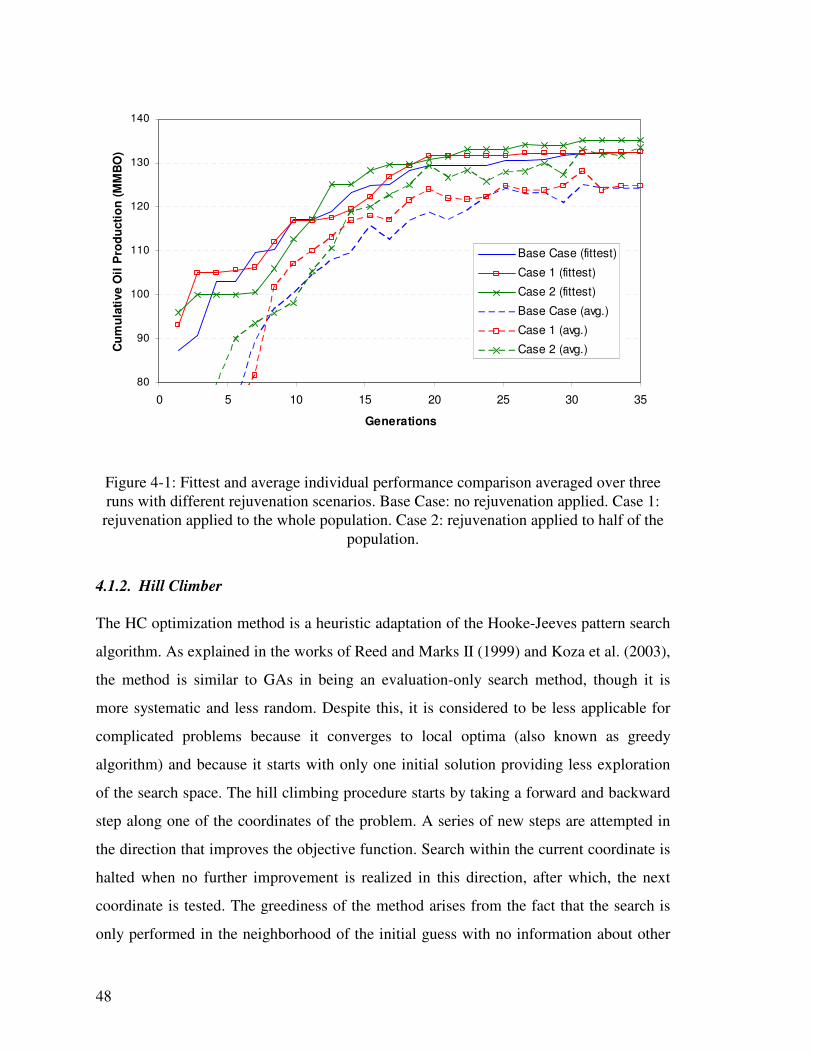
48
80
90
100
110
120
130
140
0 5 10 15 20 25 30 35
Generations
Cu
mu
lati
ve O
il P
rod
ucti
on
(M
MB
O)
Base Case (fittest)
Case 1 (fittest)
Case 2 (fittest)
Base Case (avg.)
Case 1 (avg.)
Case 2 (avg.)
Figure 4-1: Fittest and average individual performance comparison averaged over three
runs with different rejuvenation scenarios. Base Case: no rejuvenation applied. Case 1:
rejuvenation applied to the whole population. Case 2: rejuvenation applied to half of the
population.
4.1.2. Hill Climber
The HC optimization method is a heuristic adaptation of the Hooke-Jeeves pattern search
algorithm. As explained in the works of Reed and Marks II (1999) and Koza et al. (2003),
the method is similar to GAs in being an evaluation-only search method, though it is
more systematic and less random. Despite this, it is considered to be less applicable for
complicated problems because it converges to local optima (also known as greedy
algorithm) and because it starts with only one initial solution providing less exploration
of the search space. The hill climbing procedure starts by taking a forward and backward
step along one of the coordinates of the problem. A series of new steps are attempted in
the direction that improves the objective function. Search within the current coordinate is
halted when no further improvement is realized in this direction, after which, the next
coordinate is tested. The greediness of the method arises from the fact that the search is
only performed in the neighborhood of the initial guess with no information about other
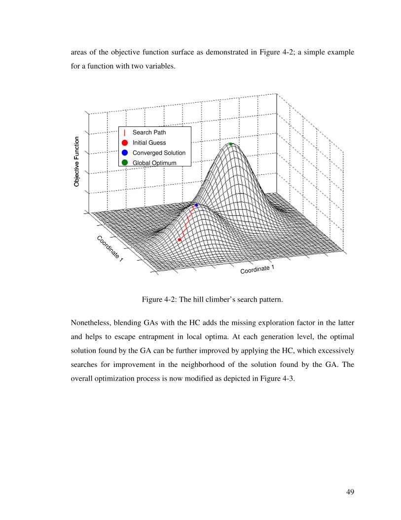
49
areas of the objective function surface as demonstrated in Figure 4-2; a simple example
for a function with two variables.
Coordinate 1
Coordinate 1
Ob
jective
Fu
nction
Search Path
Initial Guess
Converged Solution
Global Optimum
Coordinate 1
Coordinate 1
Ob
jective
Fu
nction
Search Path
Initial Guess
Converged Solution
Global Optimum
Search Path
Initial Guess
Converged Solution
Global Optimum
Figure 4-2: The hill climber’s search pattern.
Nonetheless, blending GAs with the HC adds the missing exploration factor in the latter
and helps to escape entrapment in local optima. At each generation level, the optimal
solution found by the GA can be further improved by applying the HC, which excessively
searches for improvement in the neighborhood of the solution found by the GA. The
overall optimization process is now modified as depicted in Figure 4-3.
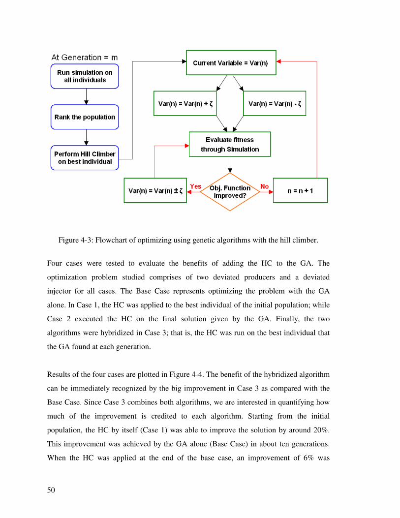
50
Figure 4-3: Flowchart of optimizing using genetic algorithms with the hill climber.
Four cases were tested to evaluate the benefits of adding the HC to the GA. The
optimization problem studied comprises of two deviated producers and a deviated
injector for all cases. The Base Case represents optimizing the problem with the GA
alone. In Case 1, the HC was applied to the best individual of the initial population; while
Case 2 executed the HC on the final solution given by the GA. Finally, the two
algorithms were hybridized in Case 3; that is, the HC was run on the best individual that
the GA found at each generation.
Results of the four cases are plotted in Figure 4-4. The benefit of the hybridized algorithm
can be immediately recognized by the big improvement in Case 3 as compared with the
Base Case. Since Case 3 combines both algorithms, we are interested in quantifying how
much of the improvement is credited to each algorithm. Starting from the initial
population, the HC by itself (Case 1) was able to improve the solution by around 20%.
This improvement was achieved by the GA alone (Base Case) in about ten generations.
When the HC was applied at the end of the base case, an improvement of 6% was
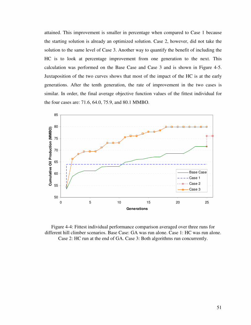
51
attained. This improvement is smaller in percentage when compared to Case 1 because
the starting solution is already an optimized solution. Case 2, however, did not take the
solution to the same level of Case 3. Another way to quantify the benefit of including the
HC is to look at percentage improvement from one generation to the next. This
calculation was performed on the Base Case and Case 3 and is shown in Figure 4-5.
Juxtaposition of the two curves shows that most of the impact of the HC is at the early
generations. After the tenth generation, the rate of improvement in the two cases is
similar. In order, the final average objective function values of the fittest individual for
the four cases are: 71.6, 64.0, 75.9, and 80.1 MMBO.
50
55
60
65
70
75
80
85
0 5 10 15 20 25
Generations
Cu
mu
lati
ve O
il P
rod
ucti
on
(M
MB
O)
Base Case
Case 1
Case 2
Case 3
Figure 4-4: Fittest individual performance comparison averaged over three runs for
different hill climber scenarios. Base Case: GA was run alone. Case 1: HC was run alone.
Case 2: HC run at the end of GA. Case 3: Both algorithms run concurrently.
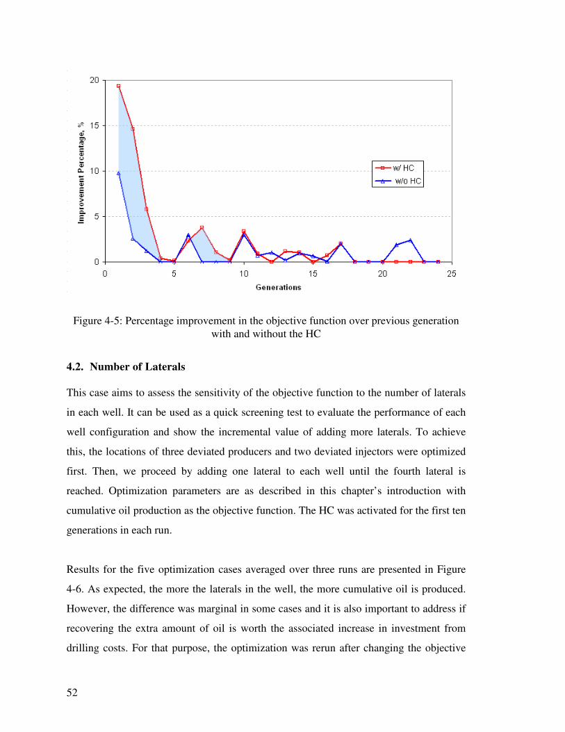
52
Figure 4-5: Percentage improvement in the objective function over previous generation
with and without the HC
4.2. Number of Laterals
This case aims to assess the sensitivity of the objective function to the number of laterals
in each well. It can be used as a quick screening test to evaluate the performance of each
well configuration and show the incremental value of adding more laterals. To achieve
this, the locations of three deviated producers and two deviated injectors were optimized
first. Then, we proceed by adding one lateral to each well until the fourth lateral is
reached. Optimization parameters are as described in this chapter’s introduction with
cumulative oil production as the objective function. The HC was activated for the first ten
generations in each run.
Results for the five optimization cases averaged over three runs are presented in Figure
4-6. As expected, the more the laterals in the well, the more cumulative oil is produced.
However, the difference was marginal in some cases and it is also important to address if
recovering the extra amount of oil is worth the associated increase in investment from
drilling costs. For that purpose, the optimization was rerun after changing the objective
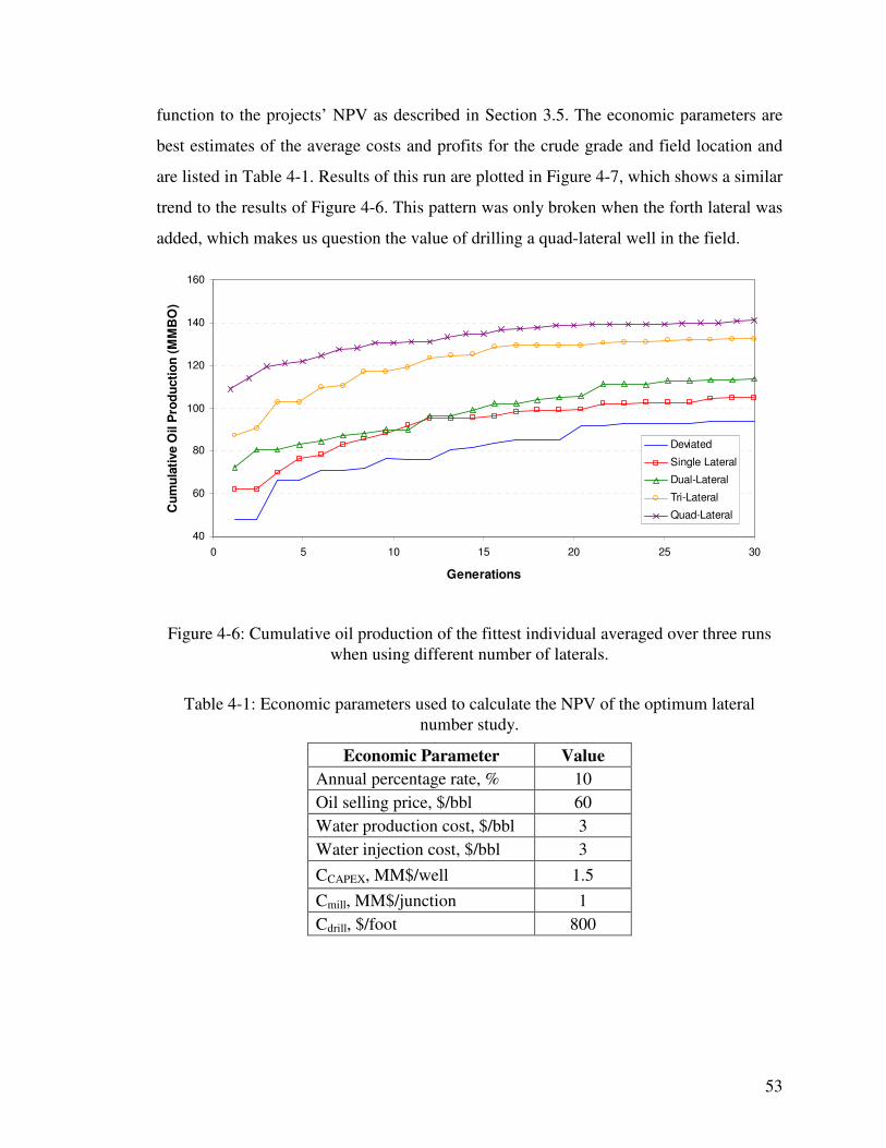
53
function to the projects’ NPV as described in Section 3.5. The economic parameters are
best estimates of the average costs and profits for the crude grade and field location and
are listed in Table 4-1. Results of this run are plotted in Figure 4-7, which shows a similar
trend to the results of Figure 4-6. This pattern was only broken when the forth lateral was
added, which makes us question the value of drilling a quad-lateral well in the field.
40
60
80
100
120
140
160
0 5 10 15 20 25 30
Generations
Cu
mu
lati
ve O
il P
rod
ucti
on
(M
MB
O)
Deviated
Single Lateral
Dual-Lateral
Tri-Lateral
Quad-Lateral
Figure 4-6: Cumulative oil production of the fittest individual averaged over three runs
when using different number of laterals.
Table 4-1: Economic parameters used to calculate the NPV of the optimum lateral
number study.
Economic Parameter Value
Annual percentage rate, % 10
Oil selling price, $/bbl 60
Water production cost, $/bbl 3
Water injection cost, $/bbl 3
CCAPEX, MM$/well 1.5
Cmill, MM$/junction 1
Cdrill, $/foot 800

54
1.50E+09
2.00E+09
2.50E+09
3.00E+09
3.50E+09
4.00E+09
4.50E+09
0 5 10 15 20 25 30 35 40
Generations
Cu
mu
lati
ve O
il P
rod
ucti
on
(M
MB
O)
Deviated
Single Lateral
Dual-Lateral
Tri-Lateral
Quad-Lateral
Figure 4-7: NPV of the fittest individual averaged over three runs when using different
number of laterals.
It is worth mentioning that the resulting well locations from each run were considerably
different with preference to particular regions that apparently have higher permeability.
The difference is attributed to the stochastic search nature of the algorithm and the
dissimilar initial population used for each run. The optimum well locations of each case
can be viewed in Figure 4-8. Most of the scenarios gave a peripheral injection pattern.
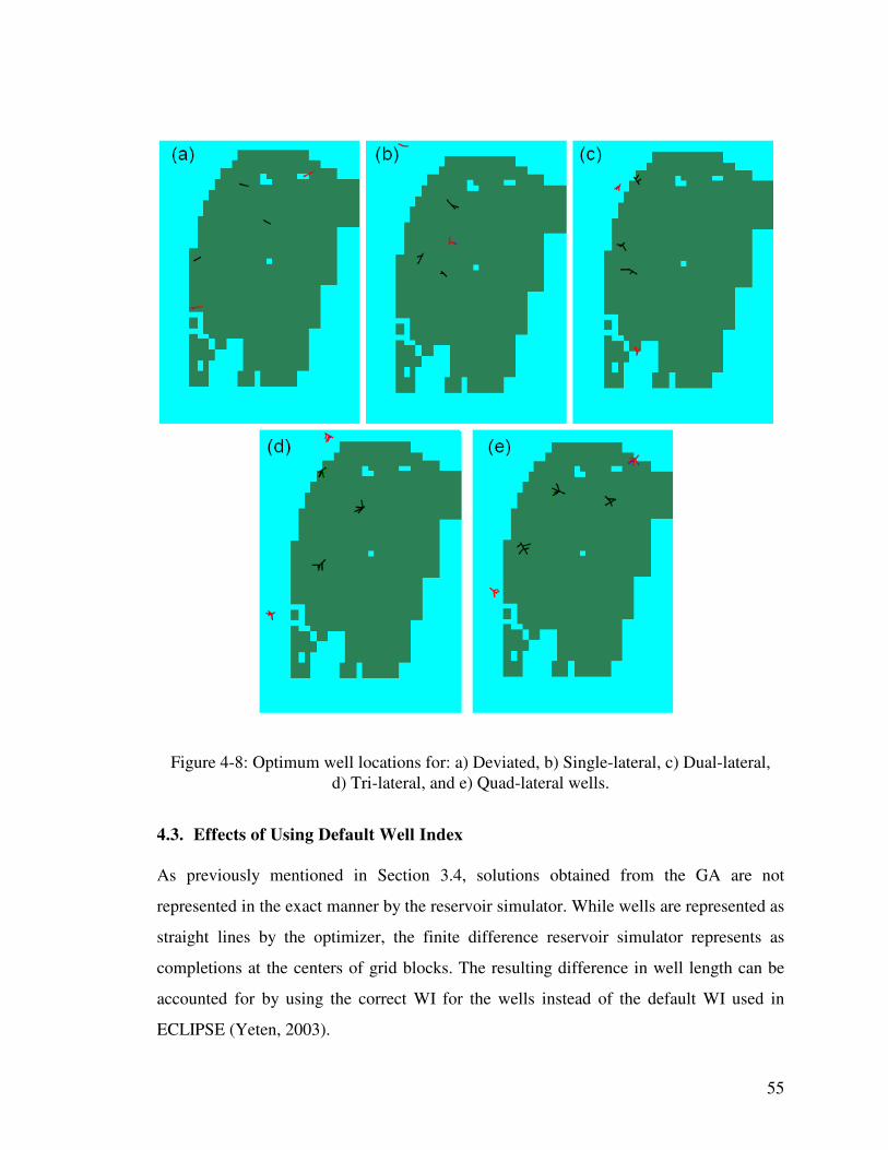
55
Figure 4-8: Optimum well locations for: a) Deviated, b) Single-lateral, c) Dual-lateral,
d) Tri-lateral, and e) Quad-lateral wells.
4.3. Effects of Using Default Well Index
As previously mentioned in Section 3.4, solutions obtained from the GA are not
represented in the exact manner by the reservoir simulator. While wells are represented as
straight lines by the optimizer, the finite difference reservoir simulator represents as
completions at the centers of grid blocks. The resulting difference in well length can be
accounted for by using the correct WI for the wells instead of the default WI used in
ECLIPSE (Yeten, 2003).
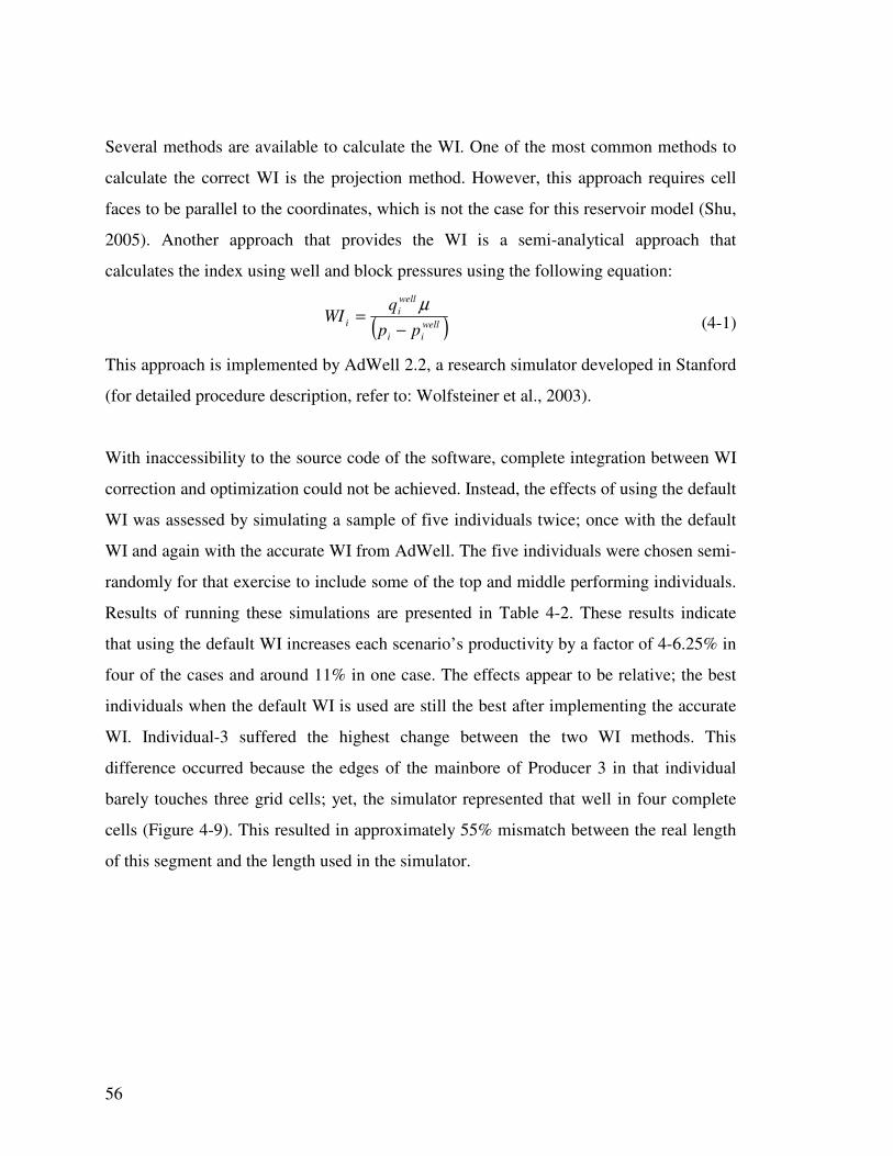
56
Several methods are available to calculate the WI. One of the most common methods to
calculate the correct WI is the projection method. However, this approach requires cell
faces to be parallel to the coordinates, which is not the case for this reservoir model (Shu,
2005). Another approach that provides the WI is a semi-analytical approach that
calculates the index using well and block pressures using the following equation:
( )well
ii
well
i
ipp
qWI
−=
µ (4-1)
This approach is implemented by AdWell 2.2, a research simulator developed in Stanford
(for detailed procedure description, refer to: Wolfsteiner et al., 2003).
With inaccessibility to the source code of the software, complete integration between WI
correction and optimization could not be achieved. Instead, the effects of using the default
WI was assessed by simulating a sample of five individuals twice; once with the default
WI and again with the accurate WI from AdWell. The five individuals were chosen semi-
randomly for that exercise to include some of the top and middle performing individuals.
Results of running these simulations are presented in Table 4-2. These results indicate
that using the default WI increases each scenario’s productivity by a factor of 4-6.25% in
four of the cases and around 11% in one case. The effects appear to be relative; the best
individuals when the default WI is used are still the best after implementing the accurate
WI. Individual-3 suffered the highest change between the two WI methods. This
difference occurred because the edges of the mainbore of Producer 3 in that individual
barely touches three grid cells; yet, the simulator represented that well in four complete
cells (Figure 4-9). This resulted in approximately 55% mismatch between the real length
of this segment and the length used in the simulator.
57
Table 4-2: Comparing cumulative oil production results for five individuals when the
default and the average WI were used.
Individual Default WI Accurate WI Difference (%)
1 130.9 123.2 6.25
2 132.5 125.4 5.66
3 129.6 116.8 10.96
4 139.3 132.2 5.37
5 124.3 119.5 4.02
Real well trajectory
Well trajectory represented in the simulator
Real well trajectory
Well trajectory represented in the simulator
Figure 4-9: Comparing the trajectory of a well that returned high difference in cumulative
oil production when the default and average WI were used.
4.4. Aquifer Uncertainty
Due to the imperfect knowledge of the reservoir geology, optimization is performed
under a lot of uncertainties. Parameters that can greatly impact the optimization outcome
include: rock and fluid properties, strength of the aquifer, and fluid contact depths.
Uncertainty propagation can assess the effects of one or multiple parameters; the more
parameters assessed, the more complicated the process. The variation in optimization
results introduced by these uncertainties can play a key role in accepting or rejecting some
of the optimized solutions. A lot of studies have attempted to study the effects of different
geological inputs on well placement optimization outcome (Guyaguler, 2002; Yeten,
2003; Onwunalu, 2006).
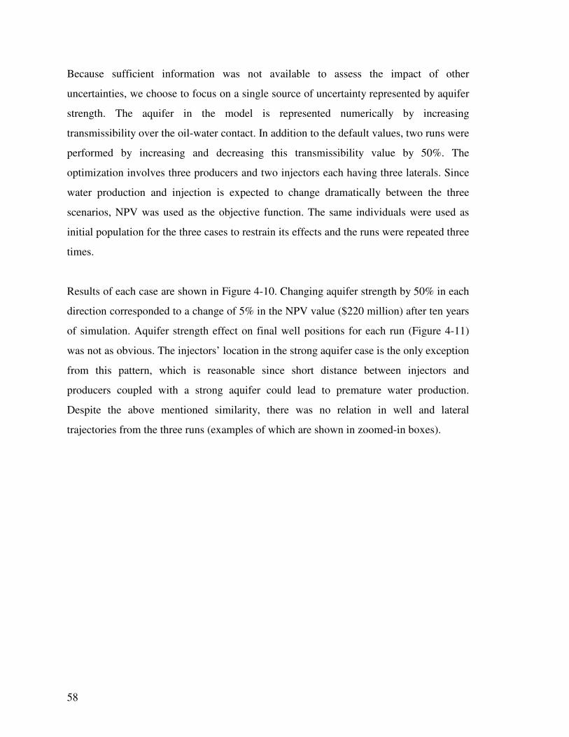
58
Because sufficient information was not available to assess the impact of other
uncertainties, we choose to focus on a single source of uncertainty represented by aquifer
strength. The aquifer in the model is represented numerically by increasing
transmissibility over the oil-water contact. In addition to the default values, two runs were
performed by increasing and decreasing this transmissibility value by 50%. The
optimization involves three producers and two injectors each having three laterals. Since
water production and injection is expected to change dramatically between the three
scenarios, NPV was used as the objective function. The same individuals were used as
initial population for the three cases to restrain its effects and the runs were repeated three
times.
Results of each case are shown in Figure 4-10. Changing aquifer strength by 50% in each
direction corresponded to a change of 5% in the NPV value ($220 million) after ten years
of simulation. Aquifer strength effect on final well positions for each run (Figure 4-11)
was not as obvious. The injectors’ location in the strong aquifer case is the only exception
from this pattern, which is reasonable since short distance between injectors and
producers coupled with a strong aquifer could lead to premature water production.
Despite the above mentioned similarity, there was no relation in well and lateral
trajectories from the three runs (examples of which are shown in zoomed-in boxes).
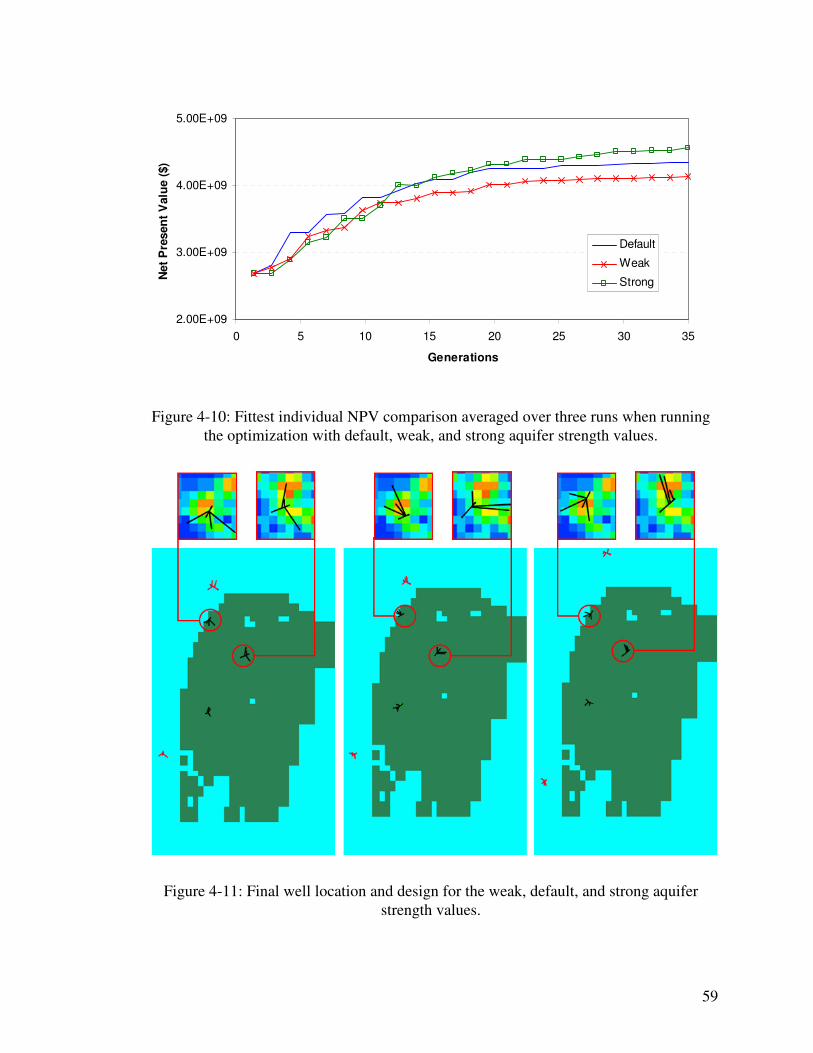
59
2.00E+09
3.00E+09
4.00E+09
5.00E+09
0 5 10 15 20 25 30 35
Generations
Net
Pre
sen
t V
alu
e (
$)
Default
Weak
Strong
Figure 4-10: Fittest individual NPV comparison averaged over three runs when running
the optimization with default, weak, and strong aquifer strength values.
Figure 4-11: Final well location and design for the weak, default, and strong aquifer
strength values.

60
However, these results are subject to projected economic model parameters used; namely,
oil price and water injection and processing cost. The significance of this statement is
illustrated by Figure 4-12, where we plot cumulative oil production and the water cut
(WC) for the fittest individual in each case. Stronger aquifer resulted in more oil
production but it also expedited the water break-through time (the WC exceeded 1% one
year earlier than the medium aquifer value and two years before the weak aquifer).
However, produced water did not exceed the field water-oil ratio constraint of 50% in any
of the cases (Vohra, 2009).
To examine the combined effect of the strength of aquifer and uncertain economic
parameters, the test matrix listed in Table 4-3 was generated by choosing two values for
oil and water price for each aquifer strength. Five of the fittest individuals were chosen
and simulations were run on them for each of the resulting 12 cases. For each solution, a
more informed decision can be deduced after looking at the mean, which indicates the
expected value of the solution; and the standard deviation for each individual, which
quantifies uncertainty in aquifer strength and economic parameters. The evaluation
criteria also depends on the adopted risk attitude. A risk averse (RA) attitude seeks to
minimize risk, while a risk seeking (RS) attitude is on the contrary. A risk neutral (RN)
attitude is somewhere in between the two. The fitness function for an individual can be
found for each attitude as defined by Yeten (2003):
F =
σ
σ
−
+
f
f
f
, (4-2)
where f is the mean and σ is the standard deviation.

61
0
30
60
90
120
150
0 500 1000 1500 2000 2500 3000 3500 4000
Time (days)
Cu
mu
lati
ve P
rod
ucti
on
(M
MB
OD
)
0
10
20
30
40
50
Wate
r C
ut
(%)
Default Prod
Weak Prod
Strong Prod
Default WC
Weak WC
Strong WC
Figure 4-12: Cumulative oil production and water cut for the optimal solutions of the
weak, default, and strong aquifer strength values
Results of completing the risk analysis procedure on the same individuals for the three
aquifer values are listed in Table 4-4. The numbers show that Indivisual-2 consistently
performs lower than the other wells (ranked bottom in 9 out of 12 cases). This individual
retains the lowest objective function regardless of the risk attitude taken. Individual-1 is
the best performer when weak and medium aquifer strengths are used. When aquifer
strength is increased further, the higher resulting water production for this individual
affects its objective function and Individual-4 becomes the fittest individual. This analysis
advises us to choose Individual-1 if we opt either a RN or RA attitude and Individual-4 if
a RS attitude is desired. Again, these two individuals are similar location wise but their
laterals’ orientation is irrelevant.
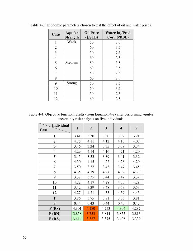
62
Table 4-3: Economic parameters chosen to test the effect of oil and water prices.
Case Aquifer Strength
Oil Price ($/STB)
Water Inj/Prod Cost ($/BBL)
1 50 3.5
2 60 3.5
3 50 2.5
4
Weak
60 2.5
5 50 3.5
6 60 3.5
7 50 2.5
8
Medium
60 2.5
9 50 3.5
10 60 3.5
11 50 2.5
12
Strong
60 2.5
Table 4-4: Objective function results (from Equation 4-2) after performing aquifer
uncertainty risk analysis on five individuals.
Individual Case 1 2 3 4 5
1 3.41 3.30 3.30 3.32 3.21
2 4.25 4.11 4.12 4.15 4.07
3 3.46 3.34 3.35 3.38 3.34
4 4.29 4.14 4.16 4.21 4.20
5 3.45 3.33 3.39 3.41 3.32
6 4.30 4.15 4.22 4.26 4.20
7 3.50 3.37 3.43 3.47 3.45
8 4.35 4.19 4.27 4.32 4.33
9 3.37 3.35 3.44 3.47 3.39
10 4.22 4.17 4.28 4.33 4.29
11 3.42 3.39 3.48 3.53 3.53
12 4.27 4.21 4.33 4.39 4.43
f 3.86 3.75 3.81 3.86 3.81
σ 0.44 0.43 0.44 0.45 0.47
F (RS) 4.301 4.180 4.253 4.304 4.287
F (RN) 3.858 3.753 3.814 3.855 3.813
F (RA) 3.414 3.327 3.375 3.406 3.339

63
4.5. Results of the Fine Model
Using the upscaled model in previous sections allowed us to conduct several tests to
evaluate the optimization algorithm within a reasonable time. If the fine model was to be
used instead, optimization time would increase by approximately 40-fold. Time
limitations in reservoir management would not always tolerate such a long period of time
before making a decision. However, it is still important to see if solutions obtained from
the upscaled model are viable ones when the fine model is used, which is the main
objective of this section.
The initial solution for this optimization will be composed from the multiple solutions
already obtained from previous runs. All of these individuals have three producers and
two injectors with three laterals. In addition to the top solutions, a number of mediocre
solutions were added to the population to maintain its diversity. As this population is yet
to go through any reproduction, it is easy to compare how well its individuals perform in
the two models. Figure 4-13 demonstrates this comparison for 10 out of 30 individuals
chosen for the initial population. These ten individuals were selected to maintain the
distribution of good and mediocre solutions from the initial population. Although most
individuals that performed well in the coarse model are still considered good solutions for
the fine model, the plot clearly shows that well performance ranking is not preserved in
the two models. The upscaled model tends to result in higher cumulative production with
Individuals G and H being the only exception. Since the coarse model was obtained by
single-phase upscaling, these discrepancies might be addressed by applying near-well
upscaling.
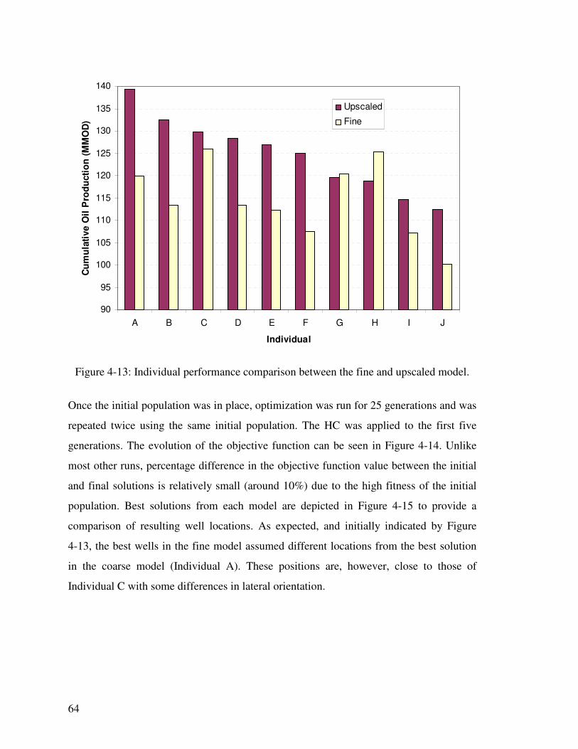
64
90
95
100
105
110
115
120
125
130
135
140
A B C D E F G H I J
Individual
Cu
mu
lati
ve O
il P
rod
ucti
on
(M
MO
D)
Upscaled
Fine
Figure 4-13: Individual performance comparison between the fine and upscaled model.
Once the initial population was in place, optimization was run for 25 generations and was
repeated twice using the same initial population. The HC was applied to the first five
generations. The evolution of the objective function can be seen in Figure 4-14. Unlike
most other runs, percentage difference in the objective function value between the initial
and final solutions is relatively small (around 10%) due to the high fitness of the initial
population. Best solutions from each model are depicted in Figure 4-15 to provide a
comparison of resulting well locations. As expected, and initially indicated by Figure
4-13, the best wells in the fine model assumed different locations from the best solution
in the coarse model (Individual A). These positions are, however, close to those of
Individual C with some differences in lateral orientation.

65
120
130
140
150
0 5 10 15 20 25
Generations
Cu
mu
lati
ve O
il P
rod
ucti
on
(M
MB
O)
Run 1
Run 2
Figure 4-14: Objective function evolution of the fittest individual for the fine model after
two optimization runs. The initial population for this optimization composed from the
fittest individuals from the upscaled model.

66
Figure 4-15: Comparison of well locations between: a) best individual in the fine model,
b) Individual C from the coarse model (ranked 3rd in the coarse model but has similar
locations to the individual in a), and c) best overall individual from the coarse model.
4.6. Concluding Remarks
This chapter focused on obtaining an optimum field development plan in terms of well
locations and design by applying the cGA to the S1 reservoir model. Completing this
exercise showed that the HC (Hill Climber) had a positive impact on the optimization
results especially at the early stages. Running the cGA with rejuvenation, another helper
tool, did not influence the performance of the algorithm for the tested case. By applying
the hybridized algorithm to this reservoir, it was found that a tri-lateral well is the most
cost efficient option as it had higher NPV than other tested well configurations. After a
base case optimum scenario was reached, uncertainty and sensitivity studies were
performed on this scenario to assess the effects of the aquifer strength, the used WI value,
and the upscaling procedure. Solutions showed little sensitivity to the first two cases but
the upscaling procedure seemed to affect the order of top solutions. A more

67
comprehensive summary of the results and conclusions of the whole study follows in the
next chapter.

69
Chapter 5
5. Conclusions and Future Work
5.1. Summary and Conclusions
With the challenging economic situations around the world, there is an ever growing
demand to examine new tools to effectively manage oil reservoirs. A challenging aspect
of reservoir management involves the optimization of nonconventional well location and
design. Cost and productivity benefits from these wells can only be realized by efficient
placement. This problem was researched in this work by comparing the performance of
binary and continuous genetic algorithms in the S1 reservoir; a carbonate reservoir in
Saudi Arabia. The optimization code was built in a way that could handle irregular grid
shapes that are common in real fields. After performing sensitivity tests on the algorithm,
optimum parameters were selected and more in-depth analysis was performed to reach an
optimum field development plan. In addition, the effects of assuming a default WI for the
well, using an upscaled reservoir model and optimizing under uncertain aquifer strength
were assessed. The major findings and conclusions from this work are:
• Both GA types (binary and continuous) were applied to the same problem. Average
results from the cGA were slightly higher and this algorithm appeared to be more
consistent when several runs were made. The reproduction and overall optimization
time was shorter in the cGA.
• Sensitivity analysis of cGA parameters revealed that early generations favor low
mutation probability, while late generations favor medium values. Dynamic mutation
was implemented to use the better mutation probability at the appropriate generation
level. This analysis also showed that better optimization results can be obtained
within a shorter period of time when dynamic population sizes are utilized.

70
• Applying an initial oil saturation constraint for producers’ midpoints tends to reduce
the number of poor individuals in the initial population, which eventually improves
the objective function values.
• The use of the HC helper tool with the GA delivered fitter final solutions. It was
found that complete hybridization of the two algorithms is more beneficial than
running one after the end of the other. Moreover, most of the improvement from this
tool was achieved in early generations. In contrast, other helper tools like rejuvenation
did not have a major impact on results.
• The effects of using the default WI were tested by simulating some individuals with
that WI value, as well as the accurate WI calculated semi-analytically. This exercise
showed the effects to be relatively small with the exception of one out of five cases.
On the other four cases, the percentage change in the objective function between the
two indices was almost constant at about 5%.
• A study of aquifer uncertainty showed that aquifer strength has an effect on the
objective function of the project but lesser effect was experienced on the location of
optimum solutions. Risk analysis was also performed to account for the effect of
economic implications of this uncertainty. This investigation showed that the choice
of solution would differ depending on the risk attitude.
• By running the optimization on the fine and coarse reservoir models, it was found that
the fittest individuals are not necessarily in agreement in both models. These
differences might be reduced by implementing near-wellbore upscaling.
• While well locations in general differed from one run to another, there was a tendency
for producers and injectors to seek particular regions of the reservoirs. The orientation
of the well laterals, on the other hand, appeared to be random. Generally speaking, the
wells were arranged in a peripheral injection with a central production system.

71
5.2. Future Work
The following suggestions are proposed for further investigation and improvement of the
nonconventional well placement optimization framework.
• The conclusions obtained are only applicable for this kind of problem and reservoir.
In order to validate them for a more general case, more simulations with different
reservoir types should be done. Additionally, models with different levels of grid
refinement should be considered to assess their impact.
• Other promising optimization techniques, such as particle swarm optimization, should
be tested on this model or on a model with similar complexity to provide comparisons
on the performance of each method.
• This study only considered one uncertainty aspect. Future studies should solve the
optimization problem under more uncertainties especially geological uncertainty.
• If a coarse model is to be used for optimization, near-wellbore upscaling should be
considered to achieve a better match between fine and upscaled optimization results.
• With the advancement in smart fields technology, future studies should consider
coupling optimization methods with real-time data acquisition to reach a more
realistic optimum solution

73
Nomenclature
Abbreviations
ANN
APR
bGA
BHP
cGA
GA
GOR
GSP
HC
MLW
MRC
NPV
OOIP
WI
artificial neural networks
annual percentage rate
binary genetic algorithm
bottom-hole pressure
continuous genetic algorithm
genetic algorithm
gas-oil ratio
general search pattern
hill climber
multilateral well
maximum reservoir contact well
net present value
original oil in place
well index
Symbols
B
C
c
F
f
i
inj
Jp
formation volume factor
constraint
compressibility
objective function
fraction
index, interest rate
injector
junction position

74
k
L
N
n
rand
P
p
prod
r
S
T
Var
Y
Zh
permeability
length
number, a randomly distributed number
normal vector, ranking of an individual
random number
probability, property
point
producer
ranking scale factor
saturation
temperature
variable
total discount years
vertical distance between heel and toe
Greek Symbols
β
Ω
µ
σ
φ
Ө
blending coefficient
search domain
viscosity
standard deviation
porosity
top-view rotation angle
Subscripts
CAPEX
d
F
g
i
capital expenditure
drilling
father
gas
index

75
M
max
mill
min
mut
o
p
r
res
select
tot
w
xo
mother
maximum
milling
minimum
mutation
oil
phase
residual, rock, relative
reservoir
selection
total
water
crossover
Superscripts
lat
mb
well
*
lateral
mainbore
well
average


77
References
Alander, J. (1992). On optimal population size of genetic algorithms. In: Proceedings
of CompEuro ’92 Computer Systems and Software Engineering, pp. 65–70.
Bittencourt, A. and Horne, R. (1997). Reservoir Development and Design
Optimization, paper SPE 38895 presented at the SPE Annual Technical
Conference and Exhibition, San Antonio, Texas, 5-8 October.
Deb, K., Agrawal, S. (1995). Simulated Binary Crossover for Continuous Search
Space, Complex Systems 9(2), pp. 115--148.
Durlofsky, L., Aziz, K., and Pan, H. (2005). AdWell Software Release Version 2.2
User Manual. Department of Energy Resources Engineering, Stanford University,
California.
Emeric, A., Silva, E., Messer, B., Almeida, L., Szwarcman, D., Pacheco, M., and
Vellasco, M. (2009). Well Placement Optimization Using a Genetic Algorithm
with Nonlinear Constraints, paper SPE 118808 presented at the SPE Reservoir
Simulation Symposium, The Woodlands, Texas, 2-4 February.
Farshi, M. (2008). Improving Genetic Algorithms for Optimum Well Placement,
Master’s Report, Department of Energy Resources Engineering, Stanford
University, California.
Fichter, D. (2000). Application of Genetic Algorithms in Portfolio Optimization for
the Oil and Gas Industry, paper SPE 62970 presented at the SPE Annual
Technical Conference and Exhibition, Dallas, Texas, 1-4 October.
GeoQuest (2007a). ECLIPSE Reference Manual 2007A. Schlumberger.
Goldberg, D. (2004). Genetic Algorithms in Search, Optimization, and Machine
Learning. Addison-Wesley, Reading.
Guyaguler, B. and Horne, R. (2001). Uncertainty Assessment of Well Placement
Optimization, paper SPE 71625 presented at the SPE Annual Technical
Conference and Exhibition, New Orleans, Louisiana, 30 September–3 October.

78
Guyaguler, B. (2002). Optimization of Well Placement and Assessment of
Uncertainty, Ph.D. dissertation, Department of Energy Resources Engineering,
Stanford University, California.
Handels, M., Zandvlier, M., Brouwer, D., and Jansen, J. (2007). Adjoint-Based Well-
Placement Optimization Under Production Constraints, paper SPE 105797
presented at the SPE Reservoir Simulation Symposium, Houston, Texas, 26-28
February.
Haupt, R. and Haupt, S. (2004). Practical Genetic Algorithms, 2nd edition, John
Wiley & Sons, New York City, New York.
Holland, J. (1992). Genetic algorithms. Scientific American, July, p. 66-72.
Horn, M., Plathey, D., and Ibrahim, O. (1997). Dual Horizontal Well Increases
Liquids Recovery in the Gulf of Thailand, paper SPE 38065 presented at the SPE
Asia Pacific Oil and Gas Conference, Kuala Lumpur, Malaysia, 14-16 April.
Isebor, O. (2009). Constrained Production Optimization with an Emphasis on
Derivative-Free Methods, Master’s Thesis, Department of Energy Resources
Engineering, Stanford University, California.
Koza, J., Bennett, F., Andre, D., and Keane, M. (1999). Genetic Programming III:
Darwinian Invention and Problem Solving. Morgan Kaufmann Publishers, San
Francisco, Calironia.
MATLAB (R2008b). MATLAB Product Help Manual. The MathWorks.
Mitchell, M. (1996). An Introduction to Genetic Algorithms. The MIT Press,
Cambridge, Massachusetts.
Montes, G., Bartolome, P., and Udias, A. (2001). The Use of Genetic Algorithms in
Well Placement Optimization, paper SPE 69439 presented at the SPE Latin
American and Caribbean Petroleum Engineering Conference, Buenos Aires,
Argentina, 25-28 March.
79
Nogueira, P. and Schiozer, D. (2009). An Efficient Methodology of Production
Strategy Optimization Based on Genetic Algorithms, paper SPE 122031 presented
at the SPE Latin American and Caribbean Petroleum Engineering Conference,
Cartagena, Colombia, 31 May-3 June.
Onwunalu, J. (2006). Optimization of Nonconventional Well Placement Using
Genetic Algorithms and Statistical Proxy, Master’s Report, Department of Energy
Resources Engineering, Stanford University, California.
Pan, Y. and Horne, R. (1998). Improved Methods for Multivariate Optimization of
Field Development Scheduling and Well Placement Design, Journal of Petroleum
Technology, December.
Radcliff, N. (1991). Formal Analysis and Random Respectful Recombination. In:
Proceedings of 4th International Conference on Genetic Algorithms, San Mateo,
CA: Morgan Kauffman.
Reed, R. and Marks II, R. (1999). Neural Smithing, Supervised Learning in
Feedforward Artificial Neural Networks. The MIT Press, Cambridge,
Massachusetts.
Saleri, N., Salamy, S., Mubarak, H., Sadler, R., Dossary, A., and Muraikhi, A. (2003).
Shaybah-220: A Maximum Reservoir Contact (MRC) Well and Its Implantations
for Developing Tight Facies Reservoirs, paper SPE 81487 presented at the SPE
13th Middle East Oil Show & Conference, Manamah, Bahrain, 5-8 April.
Shu, J. (2005). Comparison of various techniques for computing Well Index. Master’s
Thesis, Department of Energy Resources Engineering, Stanford University,
California.
Taylor, R. and Russel, R. (1997). Drilling and Completing Multilateral Horizontal
Wells in the Middle East, paper SPE 38759 presented at the SPE Annual
Technical Conference and Exhibition, San Antonio, Texas, 5-8 October.
Vohra, I. (2009). Personal Communication. Reservoir Simulation and Description
Department, Saudi Aramco.
Wang, C., Li, G., and Reynolds, A. (2007). Optimal Well Placement for Production
Optimization, paper SPE 111154 presented at the SPE Eastern Regional Meeting,
Lexington, Kentucky, 11-14 October.

80
Wikipedia, 2009, http://en.wikipedia.org
Wolfsteiner, C., Durlofsky, L., and Aziz, K. (2003). Calculation of Well Index for
Nonconventional Wells on Arbitrary Grids. Computational Geosciences, 7, pp.
61-82.
Yeten, B., Durlofsky, L. and Aziz, K. (2002). Optimization of Nonconventional Well
Type, Location and Trajectory, paper SPE 77565 presented at the SPE Annual
Technical Conference and Exhibition, San Antonio, Texas, 29 September – 2
October.
Yeten, B. (2003). Optimum Deployment of Nonconventional Wells, Ph.D. dissertation,
Department of Energy Resources Engineering, Stanford University, California.

81
Appendix A: Code and Input File
Implementation of the described optimization procedure in this work was made
possible through modularization of a number of functions coded with MATLAB 7.7.0
software. Some of the functions were modified from Farshi’s (2008) work and others
were originated by the author. All functions are included in a CD as a part of this
report. In addition, the input file that enables the user to select important optimization
parameters is included. A description of each function can be found in ‘readme.doc’ in
the main folder of the CD. A more elaborate discription and comments on the
functionality of the modules can be obtained by accessing the individual function files.