oracle8 tuning, release 8.0 - oracle documentation
TRANSCRIPT
Oracle8
Tuning
Release 8.0
December, 1997
Part No. A58246-01

Oracle8TM Tuning
Part No. A58246-01
Release 8.0
Copyright © 1997 Oracle Corporation. All Rights Reserved.
Primary Author: Rita Moran
Primary Contributors: Graham Wood, Anjo Kolk, Gary Hallmark
Contributors: Tomohiro Akiba, David Austin, Andre Bakker, Allen Brumm, Dave Colello, Carol Col-rain, Benoit Dageville, Dean Daniels, Dinesh Das, Michael Depledge, Joyce Fee, John Frazzini, JyotinGautam, Jackie Gosselin, Scott Gossett, John Graham, Todd Guay, Mike Hartstein, Scott Heisey, Alex Ho,Andrew Holdsworth, Hakan Jakobssen, Sue Jang, Robert Jenkins, Jan Klokkers, Paul Lane, Dan Leary,Tirthankar Lahiri, Juan Loaiza, Diana Lorentz, George Lumpkin, Roderick Manalac, Sheryl Maring, RaviMirchandaney, Ken Morse, Jeff Needham, Kotaro Ono, Cetin Ozbutun, Orla Parkinson, Doug Rady,Mary Rhodes, Ray Roccaforte, Hari Sankar, Leng Leng Tan, Lawrence To, Dan Tow, Peter Vasterd, SandyVenning, Radek Vingralek, Bill Waddington, Mohamed Zait
Graphic Designer: Valarie Moore
The programs are not intended for use in any nuclear, aviation, mass transit, medical, or other inher-ently dangerous applications. It shall be licensee's responsibility to take all appropriate fail-safe, backup, redundancy and other measures to ensure the safe use of such applications if the Programs areused for such purposes, and Oracle disclaims liability for any damages caused by such use of the Pro-grams.
This Program contains proprietary information of Oracle Corporation; it is provided under a licenseagreement containing restrictions on use and disclosure and is also protected by copyright patent andother intellectual property law. Reverse engineering of the software is prohibited.
The information contained in this document is subject to change without notice. If you find any problemsin the documentation, please report them to us in writing. Oracle Corporation does not warrant that thisdocument is error free.
If this Program is delivered to a U.S. Government Agency of the Department of Defense, then it is deliv-ered with Restricted Rights and the following legend is applicable:
Restricted Rights Legend Programs delivered subject to the DOD FAR Supplement are 'commercialcomputer software' and use, duplication and disclosure of the Programs shall be subject to the licensingrestrictions set forth in the applicable Oracle license agreement. Otherwise, Programs delivered subject tothe Federal Acquisition Regulations are 'restricted computer software' and use, duplication and disclo-sure of the Programs shall be subject to the restrictions in FAR 52..227-14, Rights in Data -- General,including Alternate III (June 1987). Oracle Corporation, 500 Oracle Parkway, Redwood City, CA 94065.
Oracle, SQL*Loader, Secure Network Services, and SQL*Plus are registered trademarks of OracleCorporation, Redwood Shores, California. Oracle Call Interface, Oracle8, Oracle Forms, Oracle TRACE,Oracle Expert, Oracle Enterprise Manager, Oracle Enterprise Manager Performance Pack, Oracle ParallelServer, Oracle Server Manager, Net8, PL/SQL, and Pro*C are trademarks of Oracle Corporation,Redwood Shores, California.
All other products or company names are used for identification purposes only, and may be trademarksof their respective owners.
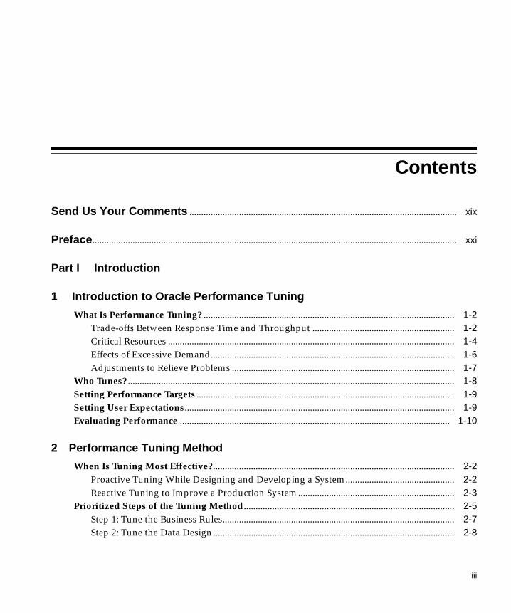
Contents
Send Us Your Comments ................................................................................................................. xix
Preface .......................................................................................................................................................... xxi
Part I Introduction
1 Introduction to Oracle Performance Tuning
What Is Performance Tuning? .......................................................................................................... 1-2Trade-offs Between Response Time and Throughput ............................................................ 1-2Critical Resources ......................................................................................................................... 1-4Effects of Excessive Demand....................................................................................................... 1-6Adjustments to Relieve Problems .............................................................................................. 1-7
Who Tunes? .......................................................................................................................................... 1-8Setting Performance Targets ............................................................................................................. 1-9Setting User Expectations.................................................................................................................. 1-9Evaluating Performance .................................................................................................................. 1-10
2 Performance Tuning Method
When Is Tuning Most Effective?...................................................................................................... 2-2Proactive Tuning While Designing and Developing a System.............................................. 2-2Reactive Tuning to Improve a Production System.................................................................. 2-3
Prioritized Steps of the Tuning Method......................................................................................... 2-5Step 1: Tune the Business Rules.................................................................................................. 2-7Step 2: Tune the Data Design...................................................................................................... 2-8
iii

Step 3: Tune the Application Design ......................................................................................... 2-9Step 4: Tune the Logical Structure of the Database ................................................................. 2-9Step 5: Tune Database Operations............................................................................................ 2-10Step 6: Tune the Access Paths ................................................................................................... 2-10Step 7: Tune Memory Allocation.............................................................................................. 2-11Step 8: Tune I/O and Physical Structure................................................................................. 2-12Step 9: Tune Resource Contention ........................................................................................... 2-12Step 10: Tune the Underlying Platform(s)............................................................................... 2-12
How to Apply the Tuning Method ................................................................................................ 2-13Set Clear Goals for Tuning ........................................................................................................ 2-13Create Minimum Repeatable Tests .......................................................................................... 2-14Test Hypotheses .......................................................................................................................... 2-14Keep Records............................................................................................................................... 2-14Avoid Common Errors .............................................................................................................. 2-15Stop Tuning When the Objectives Are Met ............................................................................ 2-16Demonstrate Meeting the Objectives ....................................................................................... 2-16
3 Diagnosing Performance Problems in an Existing System
Tuning Factors for a Well-Designed Existing System.................................................................. 3-2Insufficient CPU .................................................................................................................................. 3-5Insufficient Memory ........................................................................................................................... 3-5Insufficient I/O .................................................................................................................................... 3-6Network Constraints .......................................................................................................................... 3-7Software Constraints .......................................................................................................................... 3-7
4 Overview of Diagnostic Tools
Sources of Data for Tuning ............................................................................................................... 4-2Data Volumes ................................................................................................................................ 4-2Online Data Dictionary ................................................................................................................ 4-3Operating System Tools............................................................................................................... 4-3Dynamic Performance Tables ..................................................................................................... 4-3SQL Trace Facility......................................................................................................................... 4-3Alert Log ........................................................................................................................................ 4-3Application Program Output...................................................................................................... 4-4Users ............................................................................................................................................... 4-4
iv
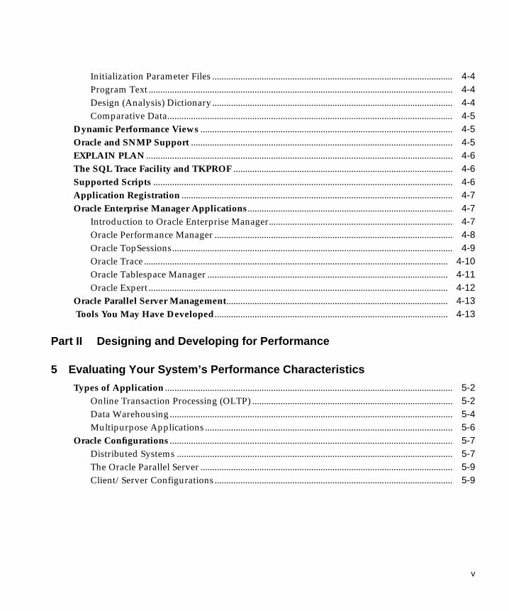
Initialization Parameter Files ...................................................................................................... 4-4Program Text................................................................................................................................. 4-4Design (Analysis) Dictionary...................................................................................................... 4-4Comparative Data......................................................................................................................... 4-5
Dynamic Performance Views ........................................................................................................... 4-5Oracle and SNMP Support ............................................................................................................... 4-5EXPLAIN PLAN .................................................................................................................................. 4-6The SQL Trace Facility and TKPROF ............................................................................................. 4-6Supported Scripts ............................................................................................................................... 4-6Application Registration ................................................................................................................... 4-7Oracle Enterprise Manager Applications....................................................................................... 4-7
Introduction to Oracle Enterprise Manager.............................................................................. 4-7Oracle Performance Manager ..................................................................................................... 4-8Oracle TopSessions....................................................................................................................... 4-9Oracle Trace................................................................................................................................. 4-10Oracle Tablespace Manager ...................................................................................................... 4-11Oracle Expert............................................................................................................................... 4-12
Oracle Parallel Server Management.............................................................................................. 4-13 Tools You May Have Developed................................................................................................... 4-13
Part II Designing and Developing for Performance
5 Evaluating Your System’s Performance Characteristics
Types of Application .......................................................................................................................... 5-2Online Transaction Processing (OLTP) ..................................................................................... 5-2Data Warehousing........................................................................................................................ 5-4Multipurpose Applications ......................................................................................................... 5-6
Oracle Configurations ........................................................................................................................ 5-7Distributed Systems ..................................................................................................................... 5-7The Oracle Parallel Server ........................................................................................................... 5-9Client/Server Configurations..................................................................................................... 5-9
v
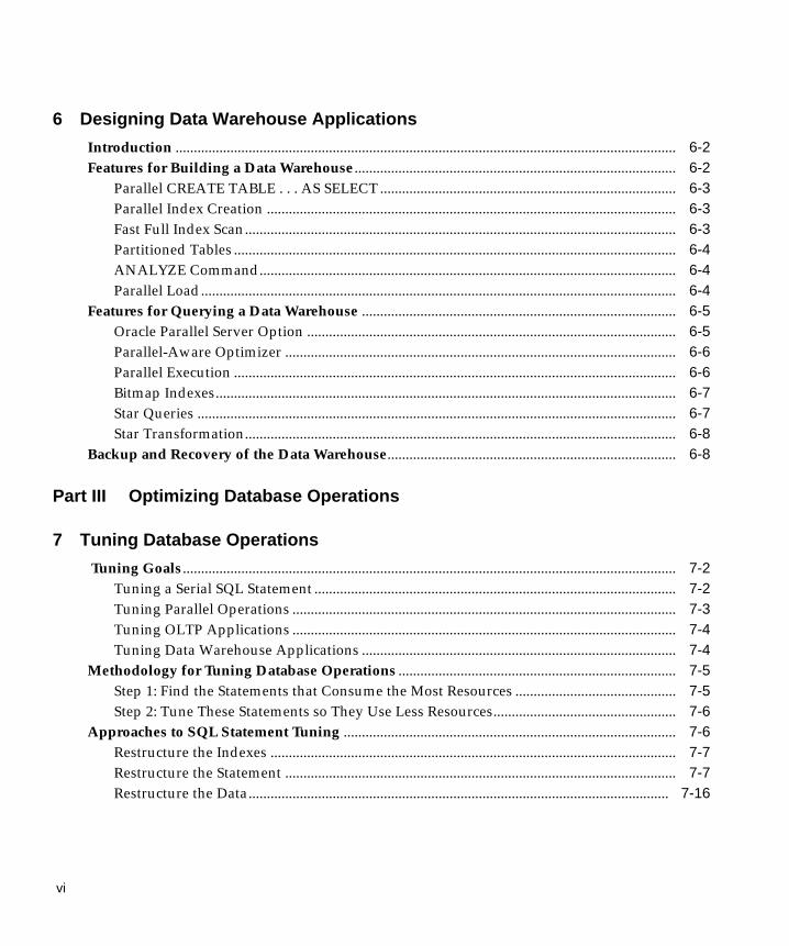
6 Designing Data Warehouse Applications
Introduction ......................................................................................................................................... 6-2Features for Building a Data Warehouse........................................................................................ 6-2
Parallel CREATE TABLE . . . AS SELECT ................................................................................. 6-3Parallel Index Creation ................................................................................................................ 6-3Fast Full Index Scan...................................................................................................................... 6-3Partitioned Tables ......................................................................................................................... 6-4ANALYZE Command.................................................................................................................. 6-4Parallel Load.................................................................................................................................. 6-4
Features for Querying a Data Warehouse ...................................................................................... 6-5Oracle Parallel Server Option ..................................................................................................... 6-5Parallel-Aware Optimizer ........................................................................................................... 6-6Parallel Execution ......................................................................................................................... 6-6Bitmap Indexes.............................................................................................................................. 6-7Star Queries ................................................................................................................................... 6-7Star Transformation...................................................................................................................... 6-8
Backup and Recovery of the Data Warehouse............................................................................... 6-8
Part III Optimizing Database Operations
7 Tuning Database Operations
Tuning Goals....................................................................................................................................... 7-2Tuning a Serial SQL Statement ................................................................................................... 7-2Tuning Parallel Operations ......................................................................................................... 7-3Tuning OLTP Applications ......................................................................................................... 7-4Tuning Data Warehouse Applications ...................................................................................... 7-4
Methodology for Tuning Database Operations ............................................................................ 7-5Step 1: Find the Statements that Consume the Most Resources ............................................ 7-5Step 2: Tune These Statements so They Use Less Resources.................................................. 7-6
Approaches to SQL Statement Tuning ........................................................................................... 7-6Restructure the Indexes ............................................................................................................... 7-7Restructure the Statement ........................................................................................................... 7-7Restructure the Data................................................................................................................... 7-16
vi
8 Optimization Modes and Hints
Using Cost-Based Optimization ...................................................................................................... 8-2When to Use the Cost-Based Approach .................................................................................... 8-2How to Use the Cost-Based Approach...................................................................................... 8-3Using Histograms for Nonuniformly Distributed Data ......................................................... 8-3Generating Statistics..................................................................................................................... 8-4Choosing a Goal for the Cost-Based Approach ....................................................................... 8-6Parameters that Affect Cost-Based Optimization Plans ......................................................... 8-7Tips for Using the Cost-Based Approach.................................................................................. 8-9
Using Rule-Based Optimization .................................................................................................... 8-10Introduction to Hints ....................................................................................................................... 8-11How to Specify Hints ....................................................................................................................... 8-11Hints for Optimization Approaches and Goals.......................................................................... 8-14
ALL_ROWS ................................................................................................................................. 8-14FIRST_ROWS .............................................................................................................................. 8-15CHOOSE ...................................................................................................................................... 8-16RULE ............................................................................................................................................ 8-16
Hints for Access Methods ............................................................................................................... 8-17FULL............................................................................................................................................. 8-17ROWID......................................................................................................................................... 8-18CLUSTER ..................................................................................................................................... 8-18HASH ........................................................................................................................................... 8-18HASH_AJ..................................................................................................................................... 8-19HASH_SJ...................................................................................................................................... 8-19INDEX .......................................................................................................................................... 8-19INDEX_ASC ................................................................................................................................ 8-21INDEX_COMBINE..................................................................................................................... 8-21INDEX_DESC.............................................................................................................................. 8-21INDEX_FFS.................................................................................................................................. 8-22MERGE_AJ .................................................................................................................................. 8-22MERGE_SJ ................................................................................................................................... 8-22AND_EQUAL ............................................................................................................................. 8-23USE_CONCAT............................................................................................................................ 8-23
vii
Hints for Join Orders........................................................................................................................ 8-24ORDERED.................................................................................................................................... 8-24STAR............................................................................................................................................. 8-24
Hints for Join Operations ................................................................................................................ 8-25USE_NL........................................................................................................................................ 8-25USE_MERGE ............................................................................................................................... 8-26USE_HASH.................................................................................................................................. 8-27DRIVING_SITE ........................................................................................................................... 8-27
Hints for Parallel Execution ............................................................................................................ 8-28PARALLEL .................................................................................................................................. 8-28NOPARALLEL............................................................................................................................ 8-29APPEND ...................................................................................................................................... 8-29NOAPPEND ................................................................................................................................ 8-30PARALLEL_INDEX ................................................................................................................... 8-30NOPARALLEL_INDEX............................................................................................................. 8-31
Additional Hints ............................................................................................................................... 8-32CACHE......................................................................................................................................... 8-32NOCACHE .................................................................................................................................. 8-32MERGE......................................................................................................................................... 8-33NO_MERGE ................................................................................................................................ 8-33PUSH_JOIN_PRED..................................................................................................................... 8-34NO_PUSH_JOIN_PRED ............................................................................................................ 8-34PUSH_SUBQ................................................................................................................................ 8-35STAR_TRANSFORMATION .................................................................................................... 8-35
Using Hints with Views................................................................................................................... 8-36Hints and Mergeable Views ...................................................................................................... 8-36Hints and Nonmergeable Views .............................................................................................. 8-37
9 Tuning Distributed Queries
Remote and Distributed Queries ..................................................................................................... 9-2Remote Data Dictionary Information ........................................................................................ 9-2Remote SQL Statements............................................................................................................... 9-3Distributed SQL Statements ........................................................................................................ 9-4EXPLAIN PLAN and SQL Decomposition............................................................................... 9-7Partition Views.............................................................................................................................. 9-8
viii
Distributed Query Restrictions...................................................................................................... 9-12Transparent Gateways...................................................................................................................... 9-13Summary: Optimizing Performance of Distributed Queries................................................... 9-14
10 Data Access Methods
Using Indexes .................................................................................................................................... 10-2When to Create Indexes............................................................................................................. 10-3Tuning the Logical Structure .................................................................................................... 10-3How to Choose Columns to Index........................................................................................... 10-5How to Choose Composite Indexes......................................................................................... 10-6How to Write Statements that Use Indexes ............................................................................ 10-7How to Write Statements that Avoid Using Indexes ............................................................ 10-8Assessing the Value of Indexes ................................................................................................ 10-8Fast Full Index Scan.................................................................................................................... 10-9Re-creating an Index ................................................................................................................ 10-10Using Existing Indexes to Enforce Uniqueness.................................................................... 10-11Using Enforced Constraints .................................................................................................... 10-11
Using Bitmap Indexes .................................................................................................................... 10-13When to Use Bitmap Indexing................................................................................................ 10-13How to Create a Bitmap Index ............................................................................................... 10-16Initialization Parameters for Bitmap Indexing..................................................................... 10-18Using Bitmap Access Plans on Regular B*-tree Indexes..................................................... 10-19Estimating Bitmap Index Size................................................................................................. 10-20Bitmap Index Restrictions ....................................................................................................... 10-23
Using Clusters ................................................................................................................................. 10-24Using Hash Clusters....................................................................................................................... 10-25
When to Use a Hash Cluster ................................................................................................... 10-25How to Use a Hash Cluster..................................................................................................... 10-26
11 Oracle8 Transaction Modes
Using Discrete Transactions ........................................................................................................... 11-2Deciding When to Use Discrete Transactions ........................................................................ 11-2How Discrete Transactions Work ............................................................................................ 11-3Errors During Discrete Transactions ....................................................................................... 11-3
ix
Usage Notes ................................................................................................................................. 11-4Example........................................................................................................................................ 11-4
Using Serializable Transactions ..................................................................................................... 11-6
12 Managing SQL and Shared PL/SQL Areas
Introduction ....................................................................................................................................... 12-2Comparing SQL Statements and PL/SQL Blocks ....................................................................... 12-2
Testing for Identical SQL Statements....................................................................................... 12-3Aspects of Standardized SQL Formatting............................................................................... 12-3
Keeping Shared SQL and PL/SQL in the Shared Pool .............................................................. 12-4Reserving Space for Large Allocations .................................................................................... 12-4Preventing Objects from Being Aged Out............................................................................... 12-4
Part IV Optimizing Oracle Instance Performances
13 Tuning CPU Resources
Understanding CPU Problems ....................................................................................................... 13-2How to Detect and Solve CPU Problems ..................................................................................... 13-4
Checking System CPU Utilization ........................................................................................... 13-4Checking Oracle CPU Utilization............................................................................................. 13-6
Solving CPU Problems by Changing System Architecture .................................................... 13-10Single Tier to Two-Tier ............................................................................................................ 13-11Multi-Tier: Using Smaller Client Machines .......................................................................... 13-11Two-Tier to Three-Tier: Using a Transaction Processing Monitor .................................... 13-12Three-Tier: Using Multiple TP Monitors............................................................................... 13-12Oracle Parallel Server ............................................................................................................... 13-13
14 Tuning Memory Allocation
Understanding Memory Allocation Issues .................................................................................. 14-2How to Detect Memory Allocation Problems ............................................................................. 14-3How to Solve Memory Allocation Problems ............................................................................... 14-3Tuning Operating System Memory Requirements .................................................................... 14-4
Reducing Paging and Swapping .............................................................................................. 14-4Fitting the System Global Area into Main Memory .............................................................. 14-5
x
Allocating Enough Memory to Individual Users .................................................................. 14-6Tuning the Redo Log Buffer ........................................................................................................... 14-7Tuning Private SQL and PL/SQL Areas........................................................................................ 14-7
Identifying Unnecessary Parse Calls ....................................................................................... 14-8Reducing Unnecessary Parse Calls .......................................................................................... 14-9
Tuning the Shared Pool ................................................................................................................. 14-11Tuning the Library Cache........................................................................................................ 14-13Tuning the Data Dictionary Cache......................................................................................... 14-19Tuning the Shared Pool with the Multithreaded Server..................................................... 14-20Tuning Reserved Space from the Shared Pool ..................................................................... 14-22
Tuning the Buffer Cache................................................................................................................ 14-26Evaluating Buffer Cache Activity by Means of the Cache Hit Ratio ................................ 14-26Raising Cache Hit Ratio by Reducing Buffer Cache Misses............................................... 14-29Removing Unnecessary Buffers when Cache Hit Ratio Is High........................................ 14-32
Tuning Multiple Buffer Pools ...................................................................................................... 14-36Overview of the Multiple Buffer Pool Feature..................................................................... 14-37When to Use Multiple Buffer Pools ....................................................................................... 14-38Tuning the Buffer Cache Using Multiple Buffer Pools ....................................................... 14-39Enabling Multiple Buffer Pools .............................................................................................. 14-39Using Multiple Buffer Pools.................................................................................................... 14-40Dictionary Views Showing Default Buffer Pools................................................................. 14-42How to Size Each Buffer Pool ................................................................................................. 14-42How to Recognize and Eliminate LRU Latch Contention.................................................. 14-45
Tuning Sort Areas ........................................................................................................................... 14-46Reallocating Memory ..................................................................................................................... 14-46Reducing Total Memory Usage .................................................................................................... 14-47
15 Tuning I/O
Understanding I/O Problems ......................................................................................................... 15-2Tuning I/O: Top Down and Bottom Up ................................................................................. 15-2Analyzing I/O Requirements ................................................................................................... 15-3Planning File Storage ................................................................................................................. 15-5Choosing Data Block Size........................................................................................................ 15-15Evaluating Device Bandwidth................................................................................................ 15-16
xi
How to Detect I/O Problems ......................................................................................................... 15-17Checking System I/O Utilization........................................................................................... 15-17Checking Oracle I/O Utilization ............................................................................................ 15-18
How to Solve I/O Problems .......................................................................................................... 15-20Reducing Disk Contention by Distributing I/O....................................................................... 15-21
What Is Disk Contention?........................................................................................................ 15-21Separating Datafiles and Redo Log Files............................................................................... 15-21Striping Table Data................................................................................................................... 15-22Separating Tables and Indexes ............................................................................................... 15-22Reducing Disk I/O Unrelated to Oracle ............................................................................... 15-22
Striping Disks.................................................................................................................................. 15-23What Is Striping?....................................................................................................................... 15-23I/O Balancing and Striping..................................................................................................... 15-23How to Stripe Disks Manually................................................................................................ 15-24How to Stripe Disks with Operating System Software....................................................... 15-25How to Do Hardware Striping with RAID........................................................................... 15-26
Avoiding Dynamic Space Management ..................................................................................... 15-26Detecting Dynamic Extension................................................................................................. 15-27Allocating Extents..................................................................................................................... 15-28Evaluating Unlimited Extents................................................................................................. 15-29Evaluating Multiple Extents.................................................................................................... 15-30Avoiding Dynamic Space Management in Rollback Segments......................................... 15-30Reducing Migrated and Chained Rows ................................................................................ 15-32Modifying the SQL.BSQ File ................................................................................................... 15-34
Tuning Sorts ..................................................................................................................................... 15-35Sorting to Memory.................................................................................................................... 15-36If You Do Sort to Disk .............................................................................................................. 15-37Optimizing Sort Performance with Temporary Tablespaces............................................. 15-38Using NOSORT to Create Indexes Without Sorting............................................................ 15-39GROUP BY NOSORT............................................................................................................... 15-39Optimizing Large Sorts with SORT_DIRECT_WRITES ..................................................... 15-40
Tuning Checkpoints ....................................................................................................................... 15-41How Checkpoints Affect Performance .................................................................................. 15-41Choosing Checkpoint Frequency ........................................................................................... 15-42Reducing the Performance Impact of a Checkpoint ............................................................ 15-42
xii
Tuning LGWR and DBWn I/O ..................................................................................................... 15-43Tuning LGWR I/O ................................................................................................................... 15-43Tuning DBWn I/O ................................................................................................................... 15-44
Configuring the Large Pool ........................................................................................................... 15-48
16 Tuning Networks
How to Detect Network Problems................................................................................................. 16-2How to Solve Network Problems .................................................................................................. 16-2
Using Array Interfaces............................................................................................................... 16-3Using Prestarted Processes........................................................................................................ 16-3Adjusting Session Data Unit Buffer Size................................................................................. 16-3Increasing the Listener Queue Size.......................................................................................... 16-3Using TCP.NODELAY............................................................................................................... 16-4Using Shared Server Processes Rather than Dedicated Server Processes .......................... 16-4Using Connection Manager ...................................................................................................... 16-4
17 Tuning the Operating System
Understanding Operating System Performance Issues ............................................................ 17-2Overview...................................................................................................................................... 17-2Operating System and Hardware Caches............................................................................... 17-2Raw Devices ................................................................................................................................ 17-3Process Schedulers...................................................................................................................... 17-3
How to Detect Operating System Problems................................................................................ 17-4How to Solve Operating System Problems ................................................................................. 17-5
Performance on UNIX-Based Systems .................................................................................... 17-5Performance on NT Systems..................................................................................................... 17-6Performance on Mainframe Computers.................................................................................. 17-6
18 Tuning Resource Contention
Understanding Contention Issues................................................................................................. 18-2How to Detect Contention Problems ............................................................................................ 18-3How to Solve Contention Problems.............................................................................................. 18-3Reducing Contention for Rollback Segments............................................................................. 18-4
Identifying Rollback Segment Contention.............................................................................. 18-4
xiii
Creating Rollback Segments...................................................................................................... 18-5Reducing Contention for Multithreaded Server Processes ...................................................... 18-6
Reducing Contention for Dispatcher Processes ..................................................................... 18-6Reducing Contention for Shared Server Processes................................................................ 18-9
Reducing Contention for Parallel Server Processes ................................................................. 18-11Identifying Contention for Parallel Server Processes .......................................................... 18-11Reducing Contention for Parallel Server Processes............................................................. 18-12
Reducing Contention for Redo Log Buffer Latches ................................................................. 18-12Detecting Contention for Space in the Redo Log Buffer ..................................................... 18-12Detecting Contention for Redo Log Buffer Latches............................................................. 18-13Examining Redo Log Activity................................................................................................. 18-14Reducing Latch Contention..................................................................................................... 18-16
Reducing Contention for the LRU Latch.................................................................................... 18-16Reducing Free List Contention..................................................................................................... 18-17
Identifying Free List Contention ............................................................................................ 18-17Adding More Free Lists ........................................................................................................... 18-18
Part V Optimizing Parallel Execution
19 Tuning Parallel Execution
Introduction to Parallel Execution Tuning ................................................................................... 19-2Step 1: Tuning System Parameters for Parallel Execution ........................................................ 19-3
Parameters Affecting Resource Consumption for All Parallel Operations........................ 19-3Parameters Affecting Resource Consumption for Parallel DML & Parallel DDL...... 19-13Parameters Enabling New Features....................................................................................... 19-16Parameters Related to I/O....................................................................................................... 19-19
Step 2: Tuning Physical Database Layout for Parallel Execution .......................................... 19-22Types of Parallelism ................................................................................................................. 19-22Striping Data.............................................................................................................................. 19-24Partitioning Data....................................................................................................................... 19-31Determining the Degree of Parallelism ................................................................................. 19-32Populating the Database Using Parallel Load...................................................................... 19-33Setting Up Temporary Tablespaces for Parallel Sort and Hash Join................................. 19-40
xiv
Creating Indexes in Parallel .................................................................................................... 19-41Additional Considerations for Parallel DML Only ............................................................. 19-42
Step 3: Analyzing Data .................................................................................................................. 19-45
20 Understanding Parallel Execution Performance Issues
Understanding Parallel Execution Performance Issues ............................................................ 20-2The Formula for Memory, Users, and Parallel Server Processes......................................... 20-2Setting Buffer Pool Size for Parallel Operations .................................................................... 20-4How to Balance the Formula .................................................................................................... 20-5Examples: Balancing Memory, Users, and Processes............................................................ 20-8Parallel Execution Space Management Issues...................................................................... 20-12Optimizing Parallel Execution on Oracle Parallel Server................................................... 20-13
Parallel Execution Tuning Techniques ....................................................................................... 20-17Overriding the Default Degree of Parallelism...................................................................... 20-17Rewriting SQL Statements ...................................................................................................... 20-18Creating and Populating Tables in Parallel .......................................................................... 20-19Creating Indexes in Parallel .................................................................................................... 20-20Refreshing Tables in Parallel................................................................................................... 20-22Using Hints with Cost Based Optimization ......................................................................... 20-24Tuning Parallel Insert Performance ....................................................................................... 20-25
21 Diagnosing Parallel Execution Performance Problems
Diagnosing Problems....................................................................................................................... 21-2Is There Regression?................................................................................................................... 21-4Is There a Plan Change?............................................................................................................. 21-4Is There a Parallel Plan?............................................................................................................. 21-4Is There a Serial Plan? ................................................................................................................ 21-5Is There Parallel Execution? ...................................................................................................... 21-5Is There Skew?............................................................................................................................. 21-6
Executing Parallel SQL Statements ............................................................................................... 21-7Using EXPLAIN PLAN to See How an Operation Is Parallelized .......................................... 21-8Using the Dynamic Performance Views..................................................................................... 21-10
V$FILESTAT.............................................................................................................................. 21-10V$PARAMETER ....................................................................................................................... 21-10V$PQ_SESSTAT........................................................................................................................ 21-10
xv
V$PQ_SLAVE............................................................................................................................ 21-11V$PQ_SYSSTAT........................................................................................................................ 21-11V$PQ_TQSTAT ......................................................................................................................... 21-11V$SESSTAT and V$SYSSTAT ................................................................................................. 21-12Querying the Dynamic Performance Views: Example........................................................ 21-12
Checking Operating System Statistics........................................................................................ 21-14Minimum Recovery Time.............................................................................................................. 21-14Parallel DML Restrictions ............................................................................................................. 21-15
Part VI Performance Diagnostic Tools
22 The Dynamic Performance Views
Instance-Level Views for Tuning ................................................................................................... 22-2Session-Level or Transient Views for Tuning.............................................................................. 22-3Current Statistic Value and Rate of Change ................................................................................ 22-4
Finding the Current Value of a Statistic .................................................................................. 22-4Finding the Rate of Change of a Statistic................................................................................. 22-5
23 The EXPLAIN PLAN Command
Introduction ....................................................................................................................................... 23-2Creating the Output Table............................................................................................................... 23-3Output Table Columns..................................................................................................................... 23-4
Bitmap Indexes and EXPLAIN PLAN................................................................................... 23-10INLIST ITERATOR and EXPLAIN PLAN ............................................................................ 23-11
Formatting EXPLAIN PLAN Output........................................................................................... 23-13How to Run EXPLAIN PLAN................................................................................................. 23-13Selecting PLAN_TABLE Output in Table Format ............................................................... 23-14Selecting PLAN_TABLE Output in Nested Format ............................................................ 23-15
EXPLAIN PLAN Restrictions ....................................................................................................... 23-16
24 The SQL Trace Facility and TKPROF
Introduction ....................................................................................................................................... 24-2About the SQL Trace Facility .................................................................................................... 24-2About TKPROF ........................................................................................................................... 24-3
xvi
How to Use the SQL Trace Facility and TKPROF ................................................................. 24-3Step 1: Set Initialization Parameters for Trace File Management ........................................... 24-4Step 2: Enable the SQL Trace Facility ........................................................................................... 24-5
Enabling the SQL Trace Facility for Your Current Session .................................................. 24-5Enabling the SQL Trace Facility for a Different User Session.............................................. 24-6Enabling the SQL Trace Facility for an Instance .................................................................... 24-6
Step 3: Format Trace Files with TKPROF ..................................................................................... 24-7Sample TKPROF Output ........................................................................................................... 24-8Syntax of TKPROF...................................................................................................................... 24-9TKPROF Statement Examples ................................................................................................ 24-12
Step 4: Interpret TKPROF Output ............................................................................................... 24-13Tabular Statistics....................................................................................................................... 24-13Library Cache Misses ............................................................................................................... 24-15Statement Truncation............................................................................................................... 24-16User Issuing the SQL Statement ............................................................................................. 24-16Execution Plan........................................................................................................................... 24-16Deciding Which Statements to Tune ..................................................................................... 24-17
Step 5: Store SQL Trace Facility Statistics.................................................................................. 24-18Generating the TKPROF Output SQL Script ........................................................................ 24-18Editing the TKPROF Output SQL Script............................................................................... 24-18Querying the Output Table..................................................................................................... 24-19
Avoiding Pitfalls in TKPROF Interpretation ............................................................................ 24-22Finding Which Statements Constitute the Bulk of the Load.............................................. 24-22The Argument Trap.................................................................................................................. 24-22The Read Consistency Trap .................................................................................................... 24-23The Schema Trap ...................................................................................................................... 24-23The Time Trap........................................................................................................................... 24-24The Trigger Trap....................................................................................................................... 24-25The “Correct” Version ............................................................................................................. 24-25
TKPROF Output Example............................................................................................................. 24-26Header........................................................................................................................................ 24-26Body............................................................................................................................................ 24-26Summary.................................................................................................................................... 24-33
xvii
25 Using Oracle Trace
Introduction ....................................................................................................................................... 25-2Using Oracle Trace for Server Performance Data Collection ................................................... 25-3Using Initialization Parameters to Control Oracle Trace .......................................................... 25-4
Enabling Oracle Trace Collections ........................................................................................... 25-4Determining the Event Set Which Oracle Trace Collects...................................................... 25-5
Using Stored Procedure Packages to Control Oracle Trace ...................................................... 25-6Using the Oracle Trace Command-Line Interface ...................................................................... 25-7Oracle Trace Collection Results...................................................................................................... 25-8
Oracle Trace Detail Reports....................................................................................................... 25-9Formatting Oracle Trace Data to Oracle Tables ................................................................... 25-10
26 Registering Applications
Overview............................................................................................................................................. 26-2Registering Applications ................................................................................................................. 26-2
DBMS_APPLICATION_INFO Package .................................................................................. 26-2Privileges...................................................................................................................................... 26-2
Setting the Module Name ............................................................................................................... 26-3Example........................................................................................................................................ 26-3Syntax ........................................................................................................................................... 26-3
Setting the Action Name.................................................................................................................. 26-4Example........................................................................................................................................ 26-4Syntax ........................................................................................................................................... 26-4
Setting the Client Information ....................................................................................................... 26-5Syntax ........................................................................................................................................... 26-5
Retrieving Application Information ............................................................................................. 26-6Querying V$SQLAREA ............................................................................................................. 26-6READ_MODULE Syntax........................................................................................................... 26-7READ_CLIENT_INFO Syntax .................................................................................................. 26-7
xviii

Send Us Your Comments
Oracle8 TM Tuning, Release 8.0
Part No. A58246-01
Oracle Corporation welcomes your comments and suggestions on the quality and usefulness of thispublication. Your input is an important part of the information used for revision.
■ Did you find any errors?■ Is the information clearly presented?■ Do you need more information? If so, where?■ Are the examples correct? Do you need more examples?■ What features did you like most about this manual?
If you find any errors or have any other suggestions for improvement, please indicate the chapter,section, and page number (if available). You can send comments to us in the following ways:
■ [email protected]■ FAX - 650-506-7228. Attn: Oracle8 Tuning■ postal service:
Oracle CorporationServer Technologies Documentation500 Oracle Parkway, 4OP12Redwood Shores, CA 94065U.S.A.
If you would like a reply, please give your name, address, and telephone number below.
xix

xx
Preface
You can enhance Oracle performance by adjusting database applications, the data-base itself, and the operating system. Making such adjustments is known as tuning.Proper tuning of Oracle provides the best possible database performance for yourspecific application and hardware configuration.
Note: Oracle8 Tuning contains information that describes the features and function-ality of the Oracle8 and the Oracle8 Enterprise Edition products. Oracle8 andOracle8 Enterprise Edition have the same basic features. However, severaladvanced features are available only with the Enterprise Edition, and some of theseare optional. For example, to use application failover, you must have the EnterpriseEdition and the Parallel Server Option.
For information about the differences between Oracle8 and the Oracle8 EnterpriseEdition and the features and options that are available to you, please refer to Get-ting to Know Oracle8 and the Oracle8 Enterprise Edition.
xxi
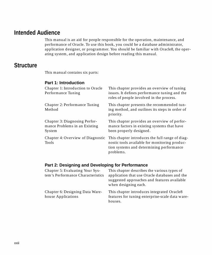
Intended AudienceThis manual is an aid for people responsible for the operation, maintenance, andperformance of Oracle. To use this book, you could be a database administrator,application designer, or programmer. You should be familiar with Oracle8, the oper-ating system, and application design before reading this manual.
StructureThis manual contains six parts:
Part 1: Introduction
Part 2: Designing and Developing for Performance
Chapter 1: Introduction to OraclePerformance Tuning
This chapter provides an overview of tuningissues. It defines performance tuning and theroles of people involved in the process.
Chapter 2: Performance TuningMethod
This chapter presents the recommended tun-ing method, and outlines its steps in order ofpriority.
Chapter 3: Diagnosing Perfor-mance Problems in an ExistingSystem
This chapter provides an overview of perfor-mance factors in existing systems that havebeen properly designed.
Chapter 4: Overview of DiagnosticTools
This chapter introduces the full range of diag-nostic tools available for monitoring produc-tion systems and determining performanceproblems.
Chapter 5: Evaluating Your Sys-tem’s Performance Characteristics
This chapter describes the various types ofapplication that use Oracle databases and thesuggested approaches and features availablewhen designing each.
Chapter 6: Designing Data Ware-house Applications
This chapter introduces integrated Oracle8features for tuning enterprise-scale data ware-houses.
xxii
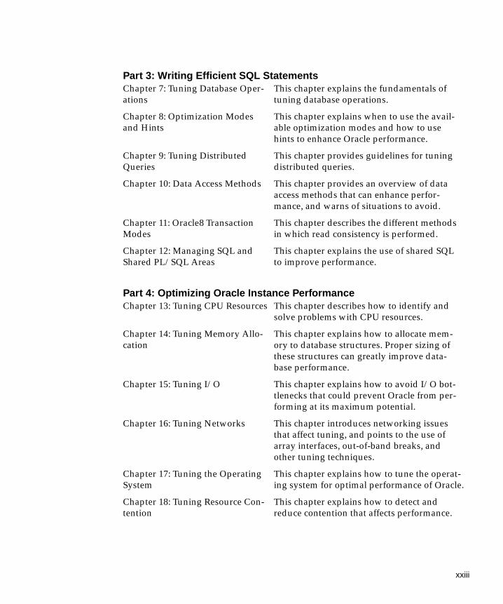
Part 3: Writing Efficient SQL Statements
Part 4: Optimizing Oracle Instance Performance
Chapter 7: Tuning Database Oper-ations
This chapter explains the fundamentals oftuning database operations.
Chapter 8: Optimization Modesand Hints
This chapter explains when to use the avail-able optimization modes and how to usehints to enhance Oracle performance.
Chapter 9: Tuning DistributedQueries
This chapter provides guidelines for tuningdistributed queries.
Chapter 10: Data Access Methods This chapter provides an overview of dataaccess methods that can enhance perfor-mance, and warns of situations to avoid.
Chapter 11: Oracle8 TransactionModes
This chapter describes the different methodsin which read consistency is performed.
Chapter 12: Managing SQL andShared PL/SQL Areas
This chapter explains the use of shared SQLto improve performance.
Chapter 13: Tuning CPU Resources This chapter describes how to identify andsolve problems with CPU resources.
Chapter 14: Tuning Memory Allo-cation
This chapter explains how to allocate mem-ory to database structures. Proper sizing ofthese structures can greatly improve data-base performance.
Chapter 15: Tuning I/O This chapter explains how to avoid I/O bot-tlenecks that could prevent Oracle from per-forming at its maximum potential.
Chapter 16: Tuning Networks This chapter introduces networking issuesthat affect tuning, and points to the use ofarray interfaces, out-of-band breaks, andother tuning techniques.
Chapter 17: Tuning the OperatingSystem
This chapter explains how to tune the operat-ing system for optimal performance of Oracle.
Chapter 18: Tuning Resource Con-tention
This chapter explains how to detect andreduce contention that affects performance.
xxiii
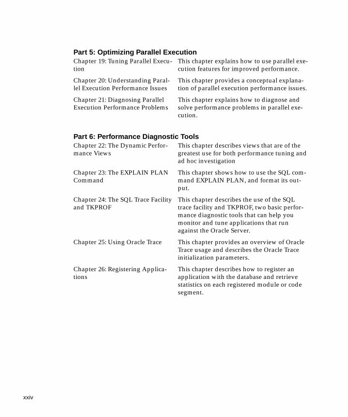
Part 5: Optimizing Parallel Execution
Part 6: Performance Diagnostic Tools
Chapter 19: Tuning Parallel Execu-tion
This chapter explains how to use parallel exe-cution features for improved performance.
Chapter 20: Understanding Paral-lel Execution Performance Issues
This chapter provides a conceptual explana-tion of parallel execution performance issues.
Chapter 21: Diagnosing ParallelExecution Performance Problems
This chapter explains how to diagnose andsolve performance problems in parallel exe-cution.
Chapter 22: The Dynamic Perfor-mance Views
This chapter describes views that are of thegreatest use for both performance tuning andad hoc investigation
Chapter 23: The EXPLAIN PLANCommand
This chapter shows how to use the SQL com-mand EXPLAIN PLAN, and format its out-put.
Chapter 24: The SQL Trace Facilityand TKPROF
This chapter describes the use of the SQLtrace facility and TKPROF, two basic perfor-mance diagnostic tools that can help youmonitor and tune applications that runagainst the Oracle Server.
Chapter 25: Using Oracle Trace This chapter provides an overview of OracleTrace usage and describes the Oracle Traceinitialization parameters.
Chapter 26: Registering Applica-tions
This chapter describes how to register anapplication with the database and retrievestatistics on each registered module or codesegment.
xxiv
Related DocumentsThis manual assumes you have already read Oracle8 Concepts, the Oracle8 Applica-tion Developer’s Guide, and Oracle8 Administrator’s Guide.
For more information about Oracle Enterprise Manager and its optional applica-tions, please see the following publications:
Oracle Enterprise Manager Concepts Guide
Oracle Enterprise Manager Administrator’s Guide
Oracle Enterprise Manager Application Developer’s Guide
Oracle Enterprise Manager: Introducing Oracle Expert
Oracle Enterprise Manager: Oracle Expert User’s Guide
Oracle Enterprise Manager Performance Monitoring User’s Guide. This manualdescribes how to use Oracle TopSessions, Oracle Monitor, and Oracle TablespaceManager.
ConventionsThis section explains the conventions used in this manual including the following:
■ text
■ syntax diagrams and notation
■ code examples
TextThis section explains the conventions used within the text:
UPPERCASE CharactersUppercase text is used to call attention to command keywords, object names,parameters, filenames, and so on.
For example, “If you create a private rollback segment, the name must be includedin the ROLLBACK_SEGMENTS parameter of the parameter file.”
Italicized CharactersItalicized words within text are book titles or emphasized words.
xxv
Syntax Diagrams and NotationThe syntax diagrams and notation in this manual show the syntax for SQL com-mands, functions, hints, and other elements. This section tells you how to read syn-tax diagrams and examples and write SQL statements based on them.
KeywordsKeywords are words that have special meanings in the SQL language. In the syntaxdiagrams in this manual, keywords appear in uppercase. You must use keywordsin your SQL statements exactly as they appear in the syntax diagram, except thatthey can be either uppercase or lowercase. For example, you must use the CREATEkeyword to begin your CREATE TABLE statements just as it appears in the CRE-ATE TABLE syntax diagram.
ParametersParameters act as place holders in syntax diagrams. They appear in lowercase.Parameters are usually names of database objects, Oracle datatype names, orexpressions. When you see a parameter in a syntax diagram, substitute an object orexpression of the appropriate type in your SQL statement. For example, to write aCREATE TABLE statement, use the name of the table you want to create, such asEMP, in place of the table parameter in the syntax diagram. (Note that parameternames appear in italics in the text.)
xxvi
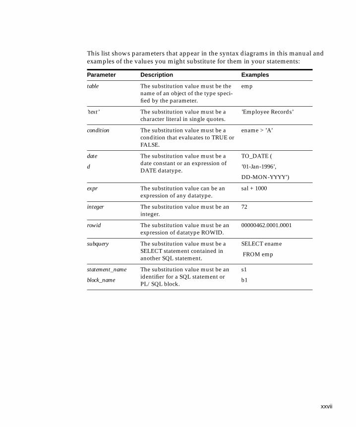
This list shows parameters that appear in the syntax diagrams in this manual andexamples of the values you might substitute for them in your statements:
Parameter Description Examples
table The substitution value must be thename of an object of the type speci-fied by the parameter.
emp
’text’ The substitution value must be acharacter literal in single quotes.
’Employee Records’
condition The substitution value must be acondition that evaluates to TRUE orFALSE.
ename > ’A’
date
d
The substitution value must be adate constant or an expression ofDATE datatype.
TO_DATE (
’01-Jan-1996’,
DD-MON-YYYY’)
expr The substitution value can be anexpression of any datatype.
sal + 1000
integer The substitution value must be aninteger.
72
rowid The substitution value must be anexpression of datatype ROWID.
00000462.0001.0001
subquery The substitution value must be aSELECT statement contained inanother SQL statement.
SELECT ename
FROM emp
statement_name
block_name
The substitution value must be anidentifier for a SQL statement orPL/SQL block.
s1
b1
xxvii
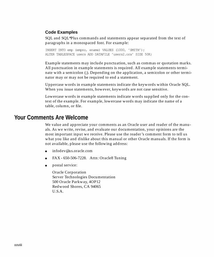
Code ExamplesSQL and SQL*Plus commands and statements appear separated from the text ofparagraphs in a monospaced font. For example:
INSERT INTO emp (empno, ename) VALUES (1000, ’SMITH’);ALTER TABLESPACE users ADD DATAFILE ’users2.ora’ SIZE 50K;
Example statements may include punctuation, such as commas or quotation marks.All punctuation in example statements is required. All example statements termi-nate with a semicolon (;). Depending on the application, a semicolon or other termi-nator may or may not be required to end a statement.
Uppercase words in example statements indicate the keywords within Oracle SQL.When you issue statements, however, keywords are not case sensitive.
Lowercase words in example statements indicate words supplied only for the con-text of the example. For example, lowercase words may indicate the name of atable, column, or file.
Your Comments Are WelcomeWe value and appreciate your comments as an Oracle user and reader of the manu-als. As we write, revise, and evaluate our documentation, your opinions are themost important input we receive. Please use the reader’s comment form to tell uswhat you like and dislike about this manual or other Oracle manuals. If the form isnot available, please use the following address:
■ FAX - 650-506-7228. Attn: Oracle8 Tuning
■ postal service:
Oracle CorporationServer Technologies Documentation500 Oracle Parkway, 4OP12Redwood Shores, CA 94065U.S.A.
xxviii
Part I
IntroductionPart I provides an overview of the concepts encountered in tuning the OracleServer. The chapters in this part are:
■ Chapter 1, “Introduction to Oracle Performance Tuning”
■ Chapter 2, “Performance Tuning Method”
■ Chapter 3, “Diagnosing Performance Problems in an Existing System”
■ Chapter 4, “Overview of Diagnostic Tools”

Introduction to Oracle Performance T
1
Introduction to Oracle Performance TuningThe Oracle Server is a sophisticated and highly tunable software product. Its flexi-bility allows you to make small adjustments that affect database performance. Bytuning your system, you can tailor its performance to best meet your needs.
This chapter gives an overview of tuning issues. Topics in this chapter include:
■ What Is Performance Tuning?
■ Who Tunes?
■ Setting Performance Targets
■ Setting User Expectations
■ Evaluating Performance
uning 1-1
What Is Performance Tuning?
What Is Performance Tuning?Performance must be built in! Performance tuning cannot be performed optimallyafter a system is put into production. To achieve performance targets of responsetime, throughput, and constraints you must tune application analysis, design, andimplementation. This section introduces some fundamental concepts:
■ Trade-offs Between Response Time and Throughput
■ Critical Resources
■ Effects of Excessive Demand
■ Adjustments to Relieve Problems
Trade-offs Between Response Time and ThroughputGoals for tuning vary, depending on the needs of the application. Online transac-tion processing (OLTP) applications define performance in terms of throughput.These applications must process thousands or even millions of very small transac-tions per day. By contrast, decision support systems (DSS applications) define per-formance in terms of response time. Demands on the database that are made byusers of DSS applications vary dramatically. One moment they may enter a querythat fetches only a few records, and the next moment they may enter a massive par-allel query that fetches and sorts hundreds of thousands of records from variousdifferent tables. Throughput becomes more of an issue when an application mustsupport a large number of users running DSS queries.
Response TimeBecause response time equals service time plus wait time, you can increase perfor-mance in two ways:
■ by reducing service time
■ by reducing wait time
Figure 1–1 illustrates ten independent tasks competing for a single resource.
1-2 Oracle8 Tuning
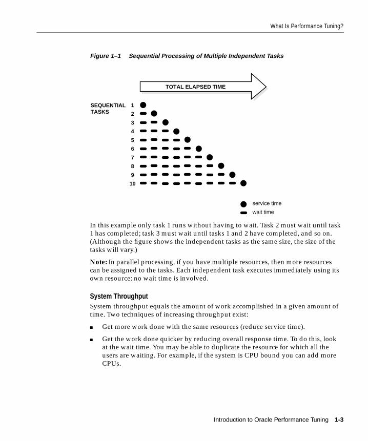
What Is Performance Tuning?
Figure 1–1 Sequential Processing of Multiple Independent Tasks
In this example only task 1 runs without having to wait. Task 2 must wait until task1 has completed; task 3 must wait until tasks 1 and 2 have completed, and so on.(Although the figure shows the independent tasks as the same size, the size of thetasks will vary.)
Note: In parallel processing, if you have multiple resources, then more resourcescan be assigned to the tasks. Each independent task executes immediately using itsown resource: no wait time is involved.
System ThroughputSystem throughput equals the amount of work accomplished in a given amount oftime. Two techniques of increasing throughput exist:
■ Get more work done with the same resources (reduce service time).
■ Get the work done quicker by reducing overall response time. To do this, lookat the wait time. You may be able to duplicate the resource for which all theusers are waiting. For example, if the system is CPU bound you can add moreCPUs.
service time
wait time
TOTAL ELAPSED TIME
SEQUENTIALTASKS
1
2
3
4
5
6
7
8
9
10
Introduction to Oracle Performance Tuning 1-3
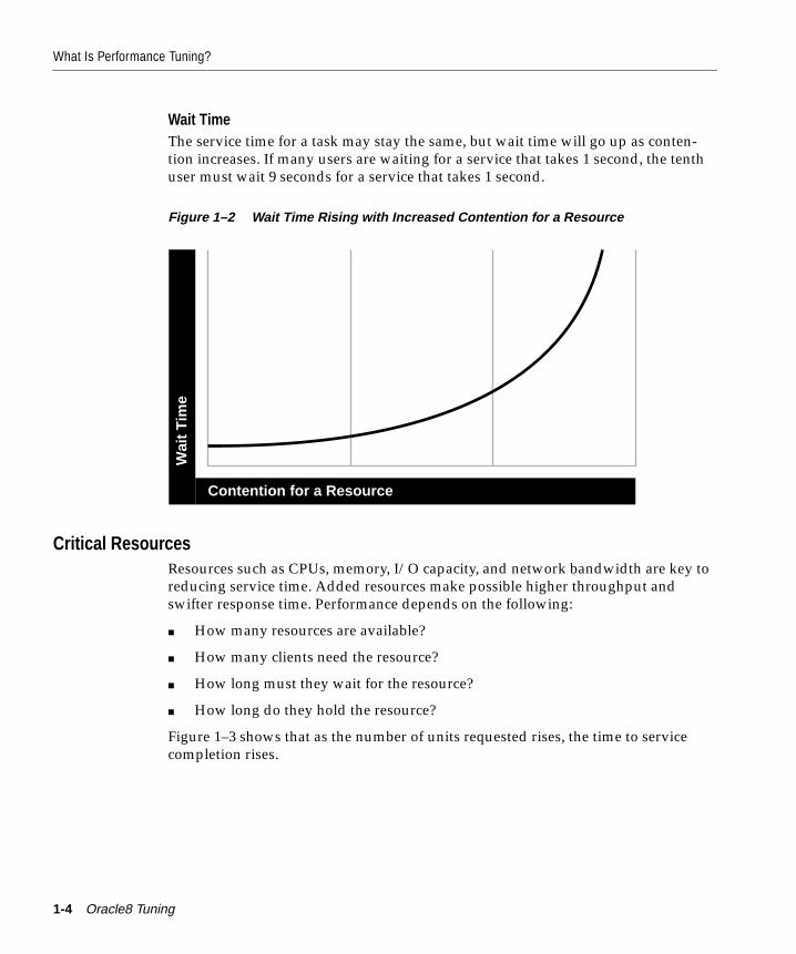
What Is Performance Tuning?
Wait TimeThe service time for a task may stay the same, but wait time will go up as conten-tion increases. If many users are waiting for a service that takes 1 second, the tenthuser must wait 9 seconds for a service that takes 1 second.
Figure 1–2 Wait Time Rising with Increased Contention for a Resource
Critical ResourcesResources such as CPUs, memory, I/O capacity, and network bandwidth are key toreducing service time. Added resources make possible higher throughput andswifter response time. Performance depends on the following:
■ How many resources are available?
■ How many clients need the resource?
■ How long must they wait for the resource?
■ How long do they hold the resource?
Figure 1–3 shows that as the number of units requested rises, the time to servicecompletion rises.
Contention for a Resource
Wai
t T
ime
1-4 Oracle8 Tuning
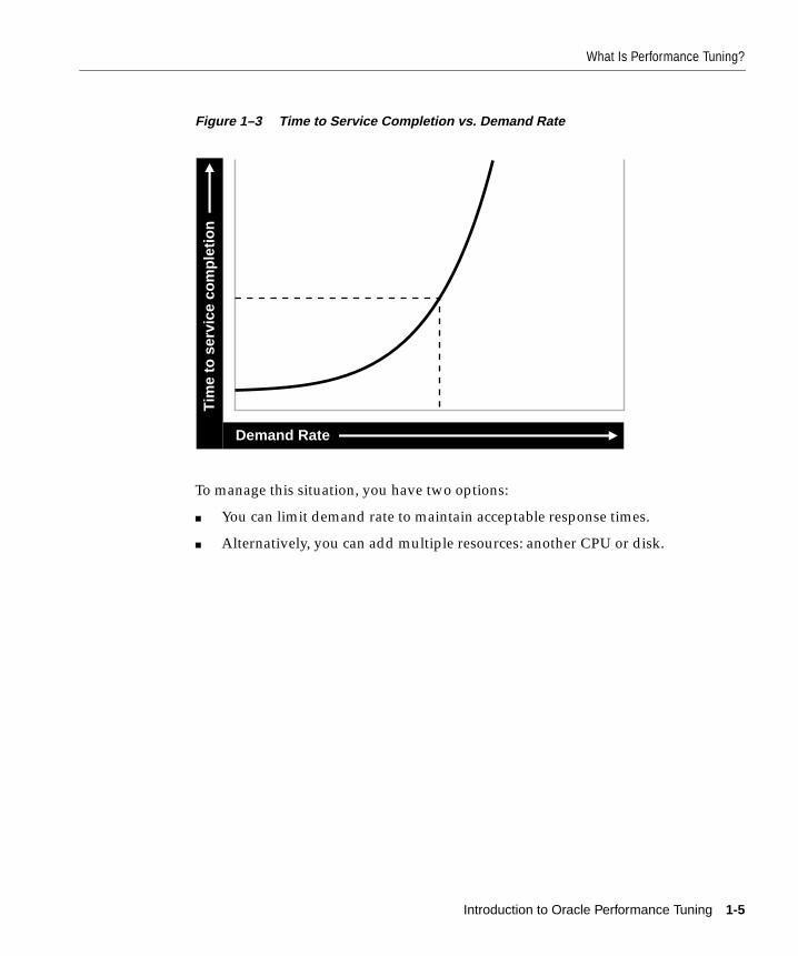
What Is Performance Tuning?
Figure 1–3 Time to Service Completion vs. Demand Rate
To manage this situation, you have two options:
■ You can limit demand rate to maintain acceptable response times.
■ Alternatively, you can add multiple resources: another CPU or disk.
Demand Rate
Tim
e to
ser
vice
co
mp
leti
on
Introduction to Oracle Performance Tuning 1-5
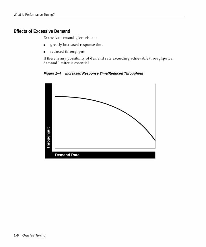
What Is Performance Tuning?
Effects of Excessive DemandExcessive demand gives rise to:
■ greatly increased response time
■ reduced throughput
If there is any possibility of demand rate exceeding achievable throughput, ademand limiter is essential.
Figure 1–4 Increased Response Time/Reduced Throughput
Demand Rate
Th
rou
gh
pu
t
1-6 Oracle8 Tuning
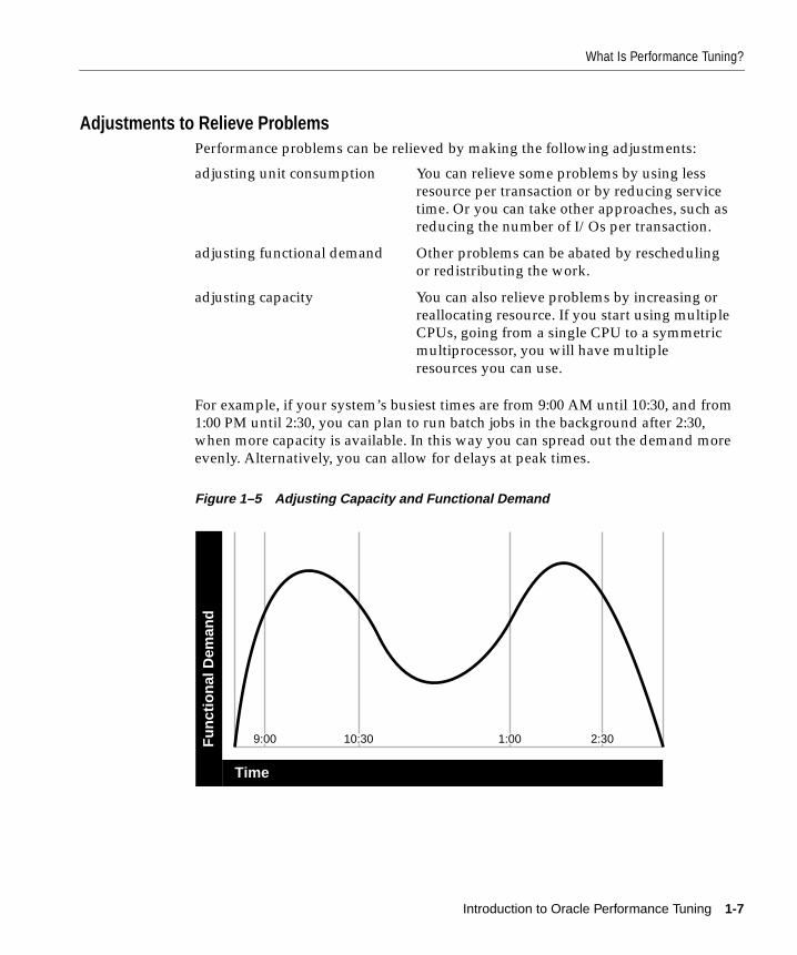
What Is Performance Tuning?
Adjustments to Relieve ProblemsPerformance problems can be relieved by making the following adjustments:
For example, if your system’s busiest times are from 9:00 AM until 10:30, and from1:00 PM until 2:30, you can plan to run batch jobs in the background after 2:30,when more capacity is available. In this way you can spread out the demand moreevenly. Alternatively, you can allow for delays at peak times.
Figure 1–5 Adjusting Capacity and Functional Demand
adjusting unit consumption You can relieve some problems by using lessresource per transaction or by reducing servicetime. Or you can take other approaches, such asreducing the number of I/Os per transaction.
adjusting functional demand Other problems can be abated by reschedulingor redistributing the work.
adjusting capacity You can also relieve problems by increasing orreallocating resource. If you start using multipleCPUs, going from a single CPU to a symmetricmultiprocessor, you will have multipleresources you can use.
Time
Fu
nct
ion
al D
eman
d
9:00 10:30 1:00 2:30
Introduction to Oracle Performance Tuning 1-7
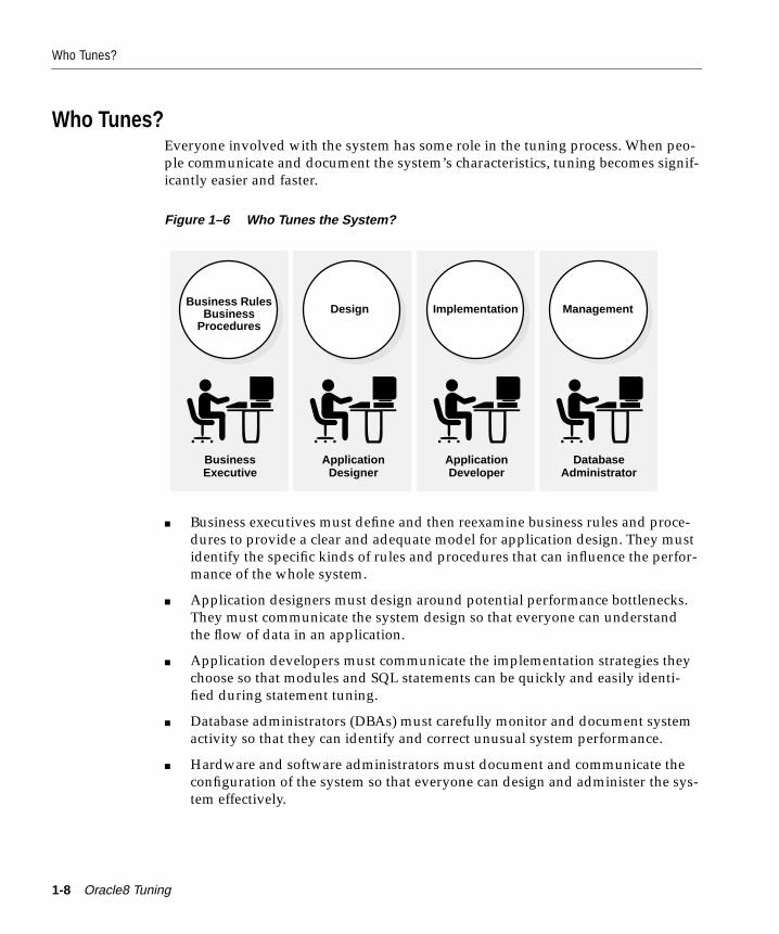
Who Tunes?
Who Tunes?Everyone involved with the system has some role in the tuning process. When peo-ple communicate and document the system’s characteristics, tuning becomes signif-icantly easier and faster.
Figure 1–6 Who Tunes the System?
■ Business executives must define and then reexamine business rules and proce-dures to provide a clear and adequate model for application design. They mustidentify the specific kinds of rules and procedures that can influence the perfor-mance of the whole system.
■ Application designers must design around potential performance bottlenecks.They must communicate the system design so that everyone can understandthe flow of data in an application.
■ Application developers must communicate the implementation strategies theychoose so that modules and SQL statements can be quickly and easily identi-fied during statement tuning.
■ Database administrators (DBAs) must carefully monitor and document systemactivity so that they can identify and correct unusual system performance.
■ Hardware and software administrators must document and communicate theconfiguration of the system so that everyone can design and administer the sys-tem effectively.
DatabaseAdministrator
ApplicationDeveloper
BusinessExecutive
Business RulesBusiness
Procedures
ApplicationDesigner
Design Implementation Management
1-8 Oracle8 Tuning
Setting User Expectations
Decisions made in application development and design have the most impact onperformance. Once the application is deployed, the database administrator usuallyhas the primary responsibility for tuning—within the limitations of the design.
See Also: Chapter 3, “Diagnosing Performance Problems in an Existing System”for keys that can help database administrators (DBAs) to identify performanceproblems and solve them reactively.
Setting Performance TargetsWhether you are designing or maintaining a system, you should set specific perfor-mance goals so that you know when to tune. You can spend needless time tuningyour system without significant gain if you attempt to alter initialization parame-ters or SQL statements without a specific goal.
When designing your system, set a specific goal: for example, an order entryresponse time of less than three seconds. If the application does not meet that goal,identify the bottleneck causing the slowdown (for example, I/O contention), deter-mine the cause, and take corrective action. During development, you should testthe application to determine whether it meets the designed performance goalsbefore deploying the application.
Tuning is usually a series of trade-offs. Once you have determined the bottlenecks,you may have to sacrifice some other areas to achieve the desired results. For exam-ple, if I/O is a problem, you may need to purchase more memory or more disks. Ifa purchase is not possible, you may have to limit the concurrency of the system toachieve the desired performance. However, if you have clearly defined goals forperformance, the decision on what to trade for higher performance is simplerbecause you have identified the most important areas.
Setting User ExpectationsApplication developers and database administrators must be careful to set appro-priate performance expectations for users. When the system carries out a particu-larly complicated operation, response time may be slower than when it isperforming a simple operation. In cases like this, the slower response time is notunreasonable.
If a DBA should promise 1-second response time, consider how this might be inter-preted. The DBA might mean that the operation would take 1 second in the data-base—and might well be able to achieve this goal. However, users querying over anetwork might experience a delay of a couple of seconds due to network traffic:they will not receive the response they expect in 1 second.
Introduction to Oracle Performance Tuning 1-9
Evaluating Performance
Evaluating PerformanceWith clearly defined performance goals, you can readily determine when perfor-mance tuning has been successful. Success depends on the functional objectivesyou have established with the user community, your ability to measure objectivelywhether or not the criteria are being met, and your ability to take corrective actionto overcome any exceptions. The rest of this tuning manual describes the tuningmethodology in detail, with information about diagnostic tools and the types of cor-rective actions you can take.
DBAs who are responsible for solving performance problems must keep a wideview of the all the factors that together determine response time. The perceivedarea of performance problems is frequently not the actual source of the problem.Users in the preceding example might conclude that there is a problem with thedatabase, whereas the actual problem is with the network. A DBA must monitorthe network, disk, CPU, and so on, to find the actual source of the problem—ratherthan simply assume that all performance problems stem from the database.
Ongoing performance monitoring enables you to maintain a well-tuned system.Keeping a history of the application’s performance over time enables you to makeuseful comparisons. With data about actual resource consumption for a range ofloads, you can conduct objective scalability studies and from these predict theresource requirements for load volumes you may anticipate in the future.
See Also: Chapter 4, “Overview of Diagnostic Tools”
1-10 Oracle8 Tuning
Performance Tuning M
2
Performance Tuning MethodMethodology is key to success in performance tuning. Different tuning strategiesoffer diminishing returns, and it is important to use the strategies with the maxi-mum gains first. Furthermore, systems with different purposes, such as onlinetransaction processing systems and decision support systems, may require differentapproaches.
Topics in this chapter include
■ When Is Tuning Most Effective?
■ Prioritized Steps of the Tuning Method
■ How to Apply the Tuning Method
See Also: "Oracle Expert" on page 4-12. Oracle Expert automates the process of col-lecting and analyzing data, and contains rules that provide database tuning recom-mendations, implementation scripts, and reports.
ethod 2-1
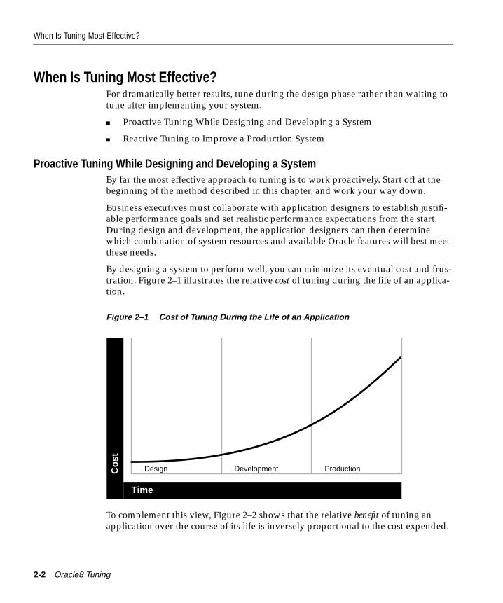
When Is Tuning Most Effective?
When Is Tuning Most Effective?For dramatically better results, tune during the design phase rather than waiting totune after implementing your system.
■ Proactive Tuning While Designing and Developing a System
■ Reactive Tuning to Improve a Production System
Proactive Tuning While Designing and Developing a SystemBy far the most effective approach to tuning is to work proactively. Start off at thebeginning of the method described in this chapter, and work your way down.
Business executives must collaborate with application designers to establish justifi-able performance goals and set realistic performance expectations from the start.During design and development, the application designers can then determinewhich combination of system resources and available Oracle features will best meetthese needs.
By designing a system to perform well, you can minimize its eventual cost and frus-tration. Figure 2–1 illustrates the relative cost of tuning during the life of an applica-tion.
Figure 2–1 Cost of Tuning During the Life of an Application
To complement this view, Figure 2–2 shows that the relative benefit of tuning anapplication over the course of its life is inversely proportional to the cost expended.
Time
Co
st
Design Development Production
2-2 Oracle8 Tuning
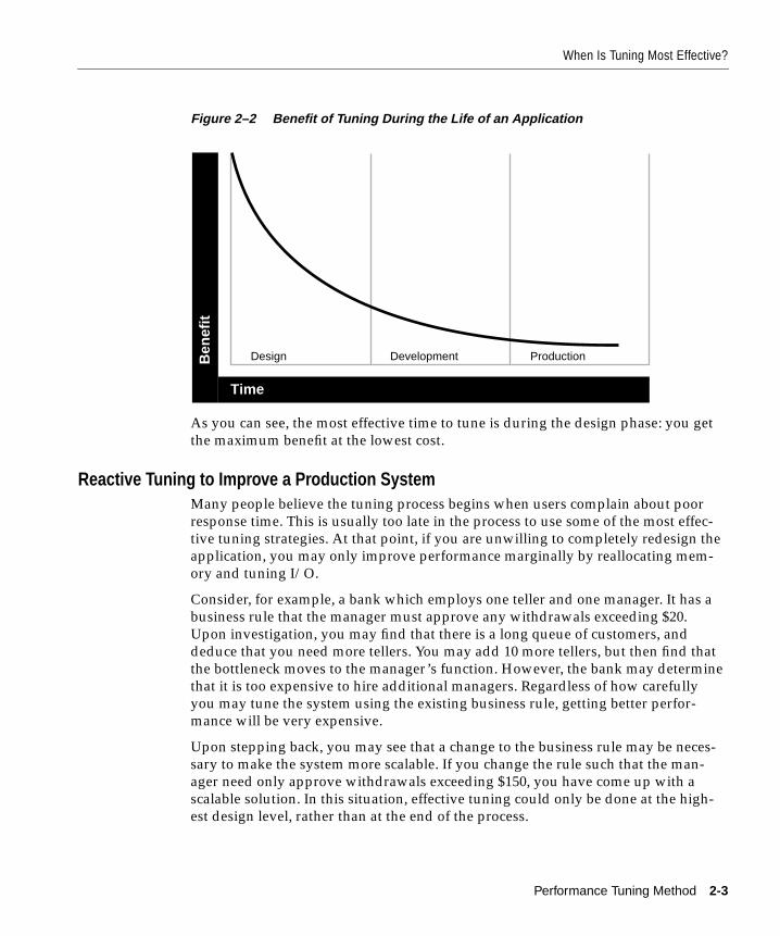
When Is Tuning Most Effective?
Figure 2–2 Benefit of Tuning During the Life of an Application
As you can see, the most effective time to tune is during the design phase: you getthe maximum benefit at the lowest cost.
Reactive Tuning to Improve a Production SystemMany people believe the tuning process begins when users complain about poorresponse time. This is usually too late in the process to use some of the most effec-tive tuning strategies. At that point, if you are unwilling to completely redesign theapplication, you may only improve performance marginally by reallocating mem-ory and tuning I/O.
Consider, for example, a bank which employs one teller and one manager. It has abusiness rule that the manager must approve any withdrawals exceeding $20.Upon investigation, you may find that there is a long queue of customers, anddeduce that you need more tellers. You may add 10 more tellers, but then find thatthe bottleneck moves to the manager’s function. However, the bank may determinethat it is too expensive to hire additional managers. Regardless of how carefullyyou may tune the system using the existing business rule, getting better perfor-mance will be very expensive.
Upon stepping back, you may see that a change to the business rule may be neces-sary to make the system more scalable. If you change the rule such that the man-ager need only approve withdrawals exceeding $150, you have come up with ascalable solution. In this situation, effective tuning could only be done at the high-est design level, rather than at the end of the process.
Time
Ben
efit
Design Development Production
Performance Tuning Method 2-3
When Is Tuning Most Effective?
It is nonetheless possible to work reactively to tune an existing production system.To take this approach, start at the bottom of the method and work your way up,finding and fixing any bottlenecks. A common goal is to make Oracle run faster onthe given platform. You may find, however, that both Oracle Server and the operat-ing system are working well: to get additional performance gains you may have totune the application or add resources. Only then can you take full advantage of themany features Oracle provides that can greatly improve performance when prop-erly used in a well-designed system.
Note that even the performance of well-designed systems can degrade with use.Ongoing tuning is therefore an important part of proper system maintenance.
See Also: Part 4: Optimizing Oracle Instance Performance, which contains chaptersthat describe in detail how to tune CPU, memory, I/O, networks, contention, andthe operating system.
Oracle8 Concepts: To find performance bottlenecks quickly and easily and determinethe corrective action for a production system, you must have a firm understandingof Oracle Server architecture and features.
2-4 Oracle8 Tuning
Prioritized Steps of the Tuning Method
Prioritized Steps of the Tuning MethodThe recommended method for tuning an Oracle database prioritizes steps in orderof diminishing returns: steps with the greatest impact on performance are listedfirst. For optimal results, therefore, tackle tuning issues in the order listed: from thedesign and development phases through instance tuning.
Step 1: Tune the Business Rules
Step 2: Tune the Data Design
Step 3: Tune the Application Design
Step 4: Tune the Logical Structure of the Database
Step 5: Tune Database Operations
Step 6: Tune the Access Paths
Step 7: Tune Memory Allocation
Step 8: Tune I/O and Physical Structure
Step 9: Tune Resource Contention
Step 10: Tune the Underlying Platform(s)
After completing the steps of the tuning method, reassess your database perfor-mance and decide whether further tuning is necessary.
Note that this is an iterative process. Performance gains made in later steps maypave the way for further improvements in earlier steps, so additional passesthrough the tuning process may be useful.
Figure 2–3 illustrates the tuning method:
Performance Tuning Method 2-5
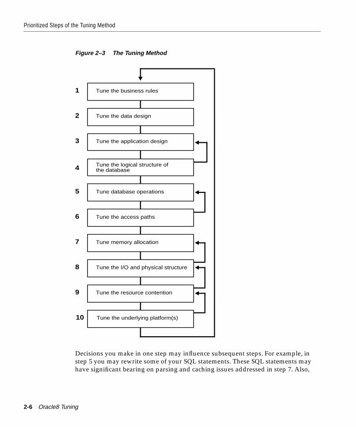
Prioritized Steps of the Tuning Method
Figure 2–3 The Tuning Method
Decisions you make in one step may influence subsequent steps. For example, instep 5 you may rewrite some of your SQL statements. These SQL statements mayhave significant bearing on parsing and caching issues addressed in step 7. Also,
Tune the data design
Tune the business rules
Tune the application design
Tune the access paths
Tune database operations
Tune the I/O and physical structure
Tune memory allocation
Tune the underlying platform(s)
Tune the resource contention
Tune the logical structure of the database
2
1
3
4
6
5
8
7
10
9
2-6 Oracle8 Tuning
Prioritized Steps of the Tuning Method
disk I/O, which is tuned in step 8, depends on the size of the buffer cache, which istuned in step 7. Although the figure shows a loop back to step 1, you may need toloop back from any step to any previous step.
Step 1: Tune the Business RulesFor optimal performance, you may have to adapt business rules. These concern thehigh-level analysis and design of an entire system. Configuration issues are consid-ered at this level, such as whether or not to use a multithreaded server system-wide. In this way, the planners ensure that the performance requirements of the sys-tem correspond directly to concrete business needs.
Performance problems encountered by the DBA may actually be caused by prob-lems in design and implementation, or by inappropriate business rules. Peoplecommonly get in too deep when they write the business functions of an applica-tion. They document an implementation, rather than simply the function that mustbe performed. If business executives use care in abstracting the business functionor requirement from the implementation, then designers have a wider field fromwhich to choose the appropriate implementation.
Consider, for example, the business function of check printing. The actual require-ment is to pay money to people; the requirement is not necessarily to print uppieces of paper. Whereas it would be very difficult to print up a million checks perday, it would be relatively easy to record that many direct deposit payments on atape which could be sent to the bank for processing.
Business rules should be consistent with realistic expectations for the number ofconcurrent users, the transaction response time, and the number of records storedonline that the system can support. For example, it would not make sense to run ahighly interactive application over slow wide area network lines.
Similarly, a company soliciting users for an Internet service might advertise 10 freehours per month for all new subscribers. If 50,000 users per day signed up for thisservice, the demand would far exceed the capacity for a client/server configura-tion. The company should instead consider using a multitier configuration. In addi-tion, the signup process must be simple: it should require only one connection fromthe user to the database, or connection to multiple databases without dedicated con-nections, making use of a multithreaded server or transaction monitor approach.
Performance Tuning Method 2-7
Prioritized Steps of the Tuning Method
Step 2: Tune the Data DesignIn the data design phase, you must determine what data is needed by your applica-tions. You need to consider what relations are important, and what their attributesare. Finally you need to structure the information to best meet performance goals.
The database design process generally undergoes a normalization stage, in whichdata is analyzed to ensure that no redundant data will be held anywhere. One factshould be stated in one and only one place in the database. Once the data is care-fully normalized, however, you may need to denormalize it for performance rea-sons. You might, for example, decide that the database should hold frequentlyrequired summary values. Rather than forcing an application to recalculate thetotal price of all the lines in a given order each time it is accessed, you might decideto include the total value of each order in the database. You could set up primarykey and foreign key indexes to access this information quickly.
Another data design consideration is the avoidance of contention on data. Considera database 1 terabyte in size, on which a thousand users access only 0.5% of thedata. This “hot spot” in the data could cause performance problems.
Try also to localize access to the data: localize it to each process, to each instance,and to each partition. Contention begins when access becomes remote, and theamount of contention determines scalability.
In Oracle Parallel Server, look for synchronization points—any point in time, orpart of an application, that must run sequentially, one process at a time. The require-ment of having sequential order numbers, for example, is a synchronization pointthat results from poor design.
Consider two Oracle8 enhancements that can help you to tune the data design toavoid contention:
■ Consider whether or not to partition your data.
■ Consider whether to use local or global indexes.
See Also: Chapter 2, “Performance Tuning Method”"Partitioning Data" on page 19-23Oracle8 Concepts for discussions of partitioning and indexes
2-8 Oracle8 Tuning
Prioritized Steps of the Tuning Method
Step 3: Tune the Application DesignBusiness executives and application designers need to translate business goals intoan effective system design. Business processes concern a particular applicationwithin a system, or a particular part of an application.
An example of intelligent process design is strategically caching data. For example,in a retail application you can select the tax rate once at the beginning of each day,and cache it within the application. In this way you avoid retrieving the same infor-mation over and over during the course of the day.
At this level also, you can consider configuration of individual processes. For exam-ple, some PC users may be accessing the central system using mobile agents,whereas other users may be directly connected. Although they are running on thesame system, the architecture is different. They may also require different mail serv-ers and different versions of the application.
Step 4: Tune the Logical Structure of the DatabaseAfter the application and the system have been designed, you can plan the logicalstructure of the database. This primarily concerns fine-tuning the index design, toensure that the data is neither over- nor under-indexed. In the data design stage(Step 2) you determine the primary and foreign key indexes. In the logical structuredesign stage you may create additional indexes to support the application.
Performance problems due to contention often involve inserts into the same blockor incorrect use of sequence numbers. Use particular care in designing the use andlocation of indexes, the sequence generator, and clusters.
See Also: "Using Indexes" on page 10-2
Performance Tuning Method 2-9
Prioritized Steps of the Tuning Method
Step 5: Tune Database OperationsSystem designers and application developers must understand Oracle’s query pro-cessing mechanism to write effective SQL statements. Chapter 8, “OptimizationModes and Hints”, discusses Oracle’s query optimizer and how to write statementsthat achieve the fastest results.
Before tuning the Oracle Server itself, be certain that your application is taking fulladvantage of the SQL language and the Oracle features designed to speed applica-tion processing. Use features and techniques such as the following based on theneeds of your application:
■ Array processing
■ The Oracle optimizer
■ The row-level lock manager
■ PL/SQL
See Also: “Part 3: Optimizing Database Operations”
Step 6: Tune the Access PathsEnsure that there is efficient access to data. Consider the use of clusters, hash clus-ters, B*-tree indexes and bitmap indexes.
Ensuring efficient access may mean adding indexes, or adding indexes for a particu-lar application and then dropping them again. It may mean revisiting your designafter you have built the database. You may want to do more normalization or cre-ate alternative indexes at this point. Upon testing the application you may find thatyou’re still not obtaining the required response time. Look for more ways toimprove the design.
See Also: Chapter 10, “Data Access Methods”
2-10 Oracle8 Tuning
Prioritized Steps of the Tuning Method
Step 7: Tune Memory AllocationAppropriate allocation of memory resources to Oracle memory structures can havea large impact on performance.
Oracle8 shared memory is allocated dynamically to the following structures, whichare all part of the shared pool. Although you explicitly set the total amount of mem-ory available in the shared pool, the system dynamically sets the size of each struc-ture contained within it:
■ The data dictionary cache
■ The library cache
■ Context areas (if running a multithreaded server)
You can explicitly set memory allocation for the following structures:
■ Buffer cache
■ Log buffer
■ Sequence caches
Proper allocation of memory resources can improve cache performance, reduceparsing of SQL statements, and reduce paging and swapping.
Process local areas include:
■ Context areas (for systems not running a multithreaded server)
■ Sort areas
■ Hash areas
Be careful not to allocate to the system global area (SGA) such a large percentage ofthe machine’s physical memory that it causes paging or swapping.
See Also: Chapter 14, “Tuning Memory Allocation”Oracle8 Concepts for information about memory structures and processes
Performance Tuning Method 2-11
Prioritized Steps of the Tuning Method
Step 8: Tune I/O and Physical StructureDisk I/O tends to reduce the performance of many software applications. OracleServer, however, is designed so that its performance need not be unduly limited byI/O. Tuning I/O and physical structure involves these procedures:
■ Distributing data so that I/O is distributed, thus avoiding disk contention
■ Storing data in data blocks for best access: setting the right number of free lists,and proper values for PCTFREE and PCTUSED
■ Creating extents large enough for your data so as to avoid dynamic extensionof tables, which would hurt high-volume OLTP applications
■ Evaluating the use of raw devices
See Also: Chapter 15, “Tuning I/O”
Step 9: Tune Resource ContentionConcurrent processing by multiple Oracle users may create contention for Oracleresources. Contention may cause processes to wait until resources are available.Take care to reduce the following kinds of contention:
■ Block contention
■ Shared pool contention
■ Lock contention
■ Pinging (in a parallel server environment)
■ Latch contention
See Also: Chapter 18, “Tuning Resource Contention”
Step 10: Tune the Underlying Platform(s)See your platform-specific Oracle documentation to investigate ways of tuning theunderlying system. For example, on UNIX-based systems you might want to tunethe following:
■ Size of the UNIX buffer cache
■ Logical volume managers
■ Memory and size for each process
See Also: Chapter 17, “Tuning the Operating System”
2-12 Oracle8 Tuning
How to Apply the Tuning Method
How to Apply the Tuning MethodThis section explains how to apply the tuning method:
■ Set Clear Goals for Tuning
■ Create Minimum Repeatable Tests
■ Test Hypotheses
■ Keep Records
■ Avoid Common Errors
■ Stop Tuning When the Objectives Are Met
■ Demonstrate Meeting the Objectives
Set Clear Goals for TuningNever begin tuning without having first established clear objectives: you cannotsucceed if there is no definition of “success.”
“Just make it go as fast as you can” may sound like an objective, but it will be verydifficult to determine whether this has been achieved. It will be even more difficultto tell whether your results have met the underlying business requirements. Amore useful statement of objectives is the following: “We need to have as many as20 operators each entering 20 orders per hour, and the packing lists producedwithin 30 minutes of the end of the shift.”
Keep your goals in mind as you consider each tuning measure; consider its perfor-mance benefits in light of your goals.
Also bear in mind that your goals may conflict. For example, to achieve best perfor-mance for a specific SQL statement, you may have to sacrifice the performance ofother SQL statements running concurrently on your database.
Performance Tuning Method 2-13
How to Apply the Tuning Method
Create Minimum Repeatable TestsCreate a series of minimum reproducible cases. For example, if you manage to iden-tify a single SQL statement that is causing a performance problem, then run boththe original and the revised version of that statement in SQL*Plus (with the SQLtrace facility or Oracle Trace enabled) so that you can see statistically the differencein performance. In many cases, a tuning effort can succeed simply by identifyingone SQL statement that was causing the performance problem.
If you must cut a 4-hour run down to 2 hours duration, you will probably find thatrepeated timings take too long. Perform your initial trials against a test environ-ment that exhibits a profile similar to the real one. For example, you could imposesome additional restrictive condition such as processing one department instead ofall 500 of them. The ideal test case will run for more than 1 minute, so that improve-ments can be seen intuitively, as well as measured using timing features. It shouldrun for less than 5 minutes, however, so that test execution does not consume anexcessive proportion of the time available.
Test HypothesesWith a minimum repeatable test established, and with a script both to conduct thetest and to summarize and report the results, you can test various hypotheses to seethe effect.
Bear in mind that Oracle’s caching algorithms mean that the first time data is vis-ited there is an additional overhead. Thus, if two approaches are tried one after theother, the second will always have a tactical advantage: data which it would other-wise have had to read from disk may be left in the cache.
Keep RecordsKeep records of the effect of each change: incorporate record keeping in the scriptbeing used to run the test. You should automate the testing process for a number ofreasons:
■ For cost effectiveness in terms of the tuner’s ability to conduct tests quickly
■ To ensure that the tests are conducted in the same way, using the same instru-mentation, for each hypothesis being tested
Anecdotal results from tests should be checked against the objective data beforebeing accepted.
2-14 Oracle8 Tuning
How to Apply the Tuning Method
Avoid Common ErrorsA common error made by inexperienced tuners is to cling to preconceived notionsabout what may be causing the problem at hand. The next most common error is totry various approaches at random.
Each time you think that you are onto something, try explaining it to someone else.Often you yourself will spot mistakes, simply from having gone through the disci-pline of articulating your ideas. For best results you should build a team of peopleto resolve performance problems. While a performance tuner can tune SQL state-ments without knowing the application in detail, the team should include someonewho does understand the application and who can validate the solutions that theSQL tuner may devise.
Avoid Rash ActionsBeware of doing something rash. Once you have a hypothesis, you may be temptedto implement it globally throughout the system and then wait to see the results.You can ruin a perfectly good system in this way!
Avoid PreconceptionsTry to avoid preconceptions when you come to a tuning problem. Get users to tellyou the symptoms they perceive—but do not expect them to know why the prob-lem exists.
One user, for example, had serious system memory problems over a long period oftime. In the morning the system ran well, but performance then dropped off veryrapidly. A consultant called in to tune the system was told that a PL/SQL memoryleak was the cause. As it turned out, this was not at all the problem. Rather, theuser had set SORT_AREA_SIZE to 10 MB on a machine with 64 MB of memory,and had 20 users. When users came on to the system, the first time they did a sortthey would get their sort area. The system thus was burdened with 200 MB of vir-tual memory and was hopelessly swapping and paging.
Many people will speculate about the cause of the problem. Ask questions of thoseaffected, and of those responsible for the system. Listen to the symptoms that usersdescribe, but do not accept prima facie their notions as to the cause!
Avoid “Hit and Hope”Avoid seizing on panaceas that may be bandied about in database folklore, such as“set the GO_FASTER parameter and everything will work faster.” Be wary of apoc-ryphal tales—such as the false notion that all tables must be in a single extent forperformance to be acceptable.
Performance Tuning Method 2-15
How to Apply the Tuning Method
Stop Tuning When the Objectives Are MetOne of the great advantages of having targets for tuning is that it becomes possibleto define success. Past a certain point, it is no longer cost effective to continue tun-ing a system.
Demonstrate Meeting the ObjectivesAs the tuner you may be confident that the performance targets have been met.You nonetheless must demonstrate this to two communities:
■ the users affected by the problem
■ those responsible for the application’s success
2-16 Oracle8 Tuning

Diagnosing Performance Problems in an Existing Sy
3
Diagnosing Performance Problems in anExisting System
This chapter provides an overview of factors affecting performance in existing sys-tems that have been properly designed. Note, however, that tuning these factorscannot compensate for poor design!
■ Tuning Factors for a Well-Designed Existing System
■ Insufficient CPU
■ Insufficient Memory
■ Insufficient I/O
■ Network Constraints
■ Software Constraints
Later chapters discuss each of these factors in depth.
stem 3-1
Tuning Factors for a Well-Designed Existing System
Tuning Factors for a Well-Designed Existing SystemThe following figure illustrates the many factors involved in Oracle system perfor-mance, when considering a well-designed existing application.
Attention: Tuning these factors is effective only after you have tuned the businessprocess and the application, as described in “Performance Tuning Method”. Tuningthese factors cannot make up for the performance gains that must be designed intothe system.
3-2 Oracle8 Tuning
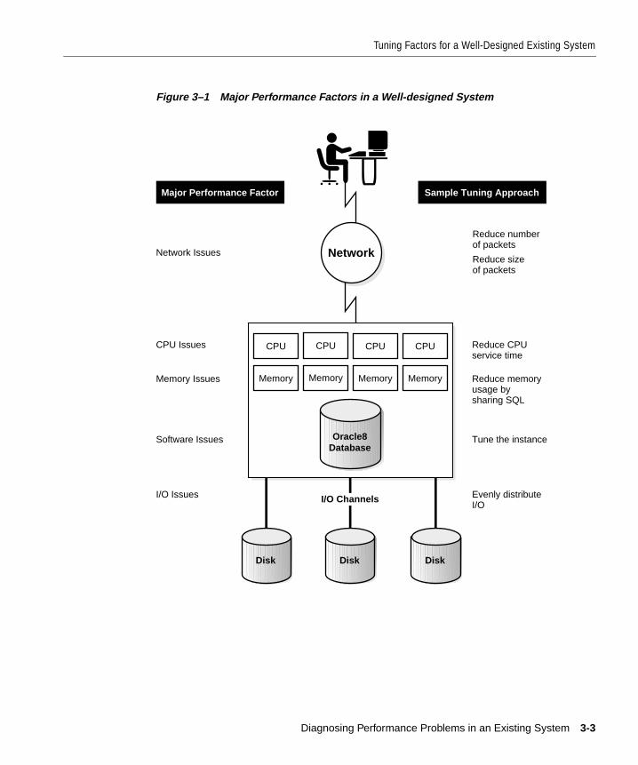
Tuning Factors for a Well-Designed Existing System
Figure 3–1 Major Performance Factors in a Well-designed System
DiskDisk Disk
I/O Channels
Tune the instance
Reduce memory usage by sharing SQL
Reduce CPUservice time
Software Issues
Memory Issues
CPU Issues
Network Issues
Reduce number of packets
Reduce size of packets
Major Performance Factor Sample Tuning Approach
Evenly distribute I/O
I/O Issues
Memory Memory Memory Memory
CPU CPU CPU CPU
Network
Oracle8Database
Diagnosing Performance Problems in an Existing System 3-3
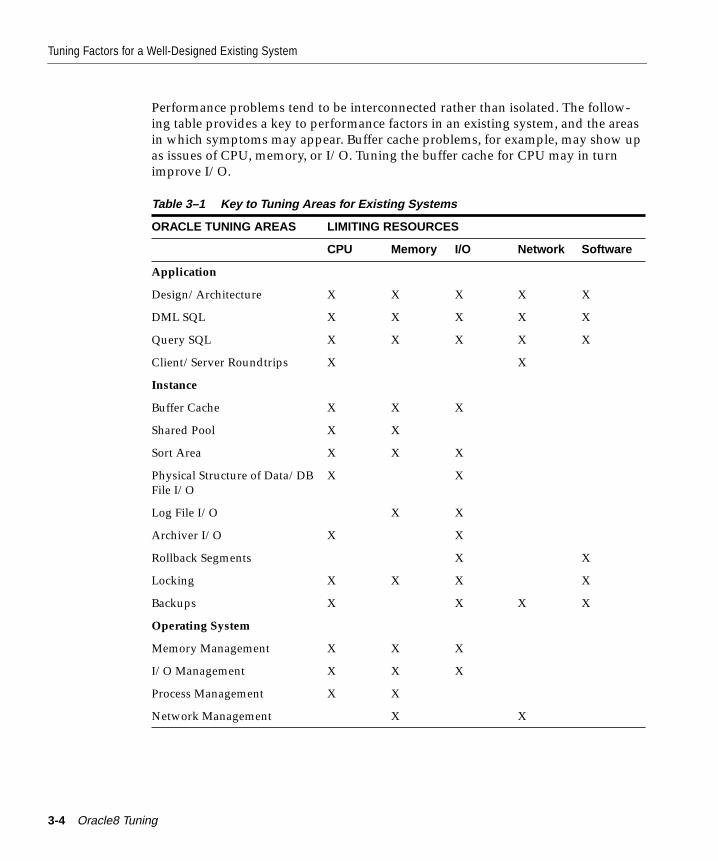
Tuning Factors for a Well-Designed Existing System
Performance problems tend to be interconnected rather than isolated. The follow-ing table provides a key to performance factors in an existing system, and the areasin which symptoms may appear. Buffer cache problems, for example, may show upas issues of CPU, memory, or I/O. Tuning the buffer cache for CPU may in turnimprove I/O.
Table 3–1 Key to Tuning Areas for Existing Systems
ORACLE TUNING AREAS LIMITING RESOURCES
CPU Memory I/O Network Software
Application
Design/Architecture X X X X X
DML SQL X X X X X
Query SQL X X X X X
Client/Server Roundtrips X X
Instance
Buffer Cache X X X
Shared Pool X X
Sort Area X X X
Physical Structure of Data/DBFile I/O
X X
Log File I/O X X
Archiver I/O X X
Rollback Segments X X
Locking X X X X
Backups X X X X
Operating System
Memory Management X X X
I/O Management X X X
Process Management X X
Network Management X X
3-4 Oracle8 Tuning
Insufficient Memory
Insufficient CPUIn a CPU-bound system, the CPU resource is completely used up, service time istoo high and you want to achieve more. Alternatively, you have too much idletime, want to achieve more, and the CPU is not completely used up. There is roomto do more: you need to determine why so much time is spent waiting.
To diagnose insufficient CPU, you must check CPU utilization by your entire sys-tem, not only utilization by Oracle Server processes. At the beginning of a workday,for example, the mail system may consume a very large amount of the availableCPU while employees check their messages. Later in the day, the mail system maybe much less heavily used, and its CPU utilization will drop accordingly.
Workload is a very important factor when evaluating your system’s level of CPUutilization. During peak workload hours, 90% CPU utilization with 10% idle andwaiting time may be understandable and acceptable; 30% utilization at a time oflow workload may also be understandable. However, if your system shows highutilization at normal workload, there is not room for peak workload. You have aCPU problem if idle time and time waiting for I/O are both close to zero (less than5%) at a normal or low workload.
See Also: Chapter 13, “Tuning CPU Resources”
Insufficient MemorySometimes a memory problem may be detected as an I/O problem. There are twokinds of memory requirements: Oracle and system. Oracle memory requirementsaffect the system requirements. Memory problems may be the cause of all the pag-ing and swapping that goes on in the machine. Make sure that your system doesnot start swapping and paging. The whole system should be able to run within thelimitations set by internal memory.
System memory requirements for non-Oracle processes plus Oracle memoryrequirements should be equal to or less than internal memory. To achieve this, youcan trim some elements of the Oracle requirements, most likely buffer cache,shared pool, or redo log buffer. On the system level you can trim the number of pro-cesses and/or the amount of memory each process uses. You can also identifywhich processes are using the most memory. One way to reduce memory usagemight be by sharing SQL.
See Also: Chapter 14, “Tuning Memory Allocation”
Diagnosing Performance Problems in an Existing System 3-5

Insufficient I/O
Insufficient I/OBe sure to distribute I/O evenly across disks and channels. I/O resources involve:
■ Channel bandwidth: number of I/O channels
■ Device bandwidth: number of disks
■ Device latency: latency will be part of your wait time
I/O problems may result from limitations of your hardware configuration. Yoursystem needs enough disks and SCSI busses to support the transaction throughputyou desire. You can evaluate the configuration by figuring the number of messagesall your disks and busses can potentially support, and comparing that to the num-ber of messages required by your peak workload.
If the response time of an I/O becomes too high, the most common problem is thatwait time has gone up (response time = service time + wait time). If wait time goesup, it means that there are too many I/O requests for this device. If service timegoes up, this normally means that the I/O requests are larger, so you write morebytes.
The different background processes (DBWR, ARCH, and so on) perform differentkinds of I/O, and each process has different I/O characteristics. Some read andwrite in the block size of the database, some read and write in larger chunks. If ser-vice time is too high, stripe the file over different devices.
Mirroring can also be a cause of I/O bottlenecks unless the data is mirrored on thesame number of disks as the database itself.
See Also: Chapter 15, “Tuning I/O”
3-6 Oracle8 Tuning
Software Constraints
Network ConstraintsNetwork constraints are similar to I/O constraints. You need to consider:
■ Network bandwidth: Each transaction requires that a certain number of pack-ets be sent over the network. If you know the number of packets required forone transaction, you can compare that to the bandwidth to determine whetheryour system is capable of supporting the desired workload.
■ Message rates: You can reduce the number of packets on the network by batch-ing them rather than sending lots of small packets.
■ Transmission time
As the number of users and the demand rises, the network can sometimes quietlybecome the bottleneck in an application. You may be spending a lot of time waitingfor network availability. Use available operating system tools to see how busy yournetwork is.
See Also: Chapter 16, “Tuning Networks”
Software ConstraintsOperating system software determines:
■ The maximum number of processes you can support
■ The maximum number of processes you can connect
Before you can tune Oracle effectively, you must ensure that the operating systemis at its peak performance. Work closely with the hardware/software system admin-istrators to ensure that Oracle is allocated the proper operating system resources.
Note: On NT systems there are no pre-set or configurable maximum numbers ofprocesses that can be supported or connected.
See Also: Operating system tuning is different for every platform. Refer to youroperating system hardware/software documentation as well as your Oracle operat-ing system-specific documentation for more information.In addition, see Chapter 17, “Tuning the Operating System”.
Diagnosing Performance Problems in an Existing System 3-7

Software Constraints
3-8 Oracle8 Tuning
Overview of Diagnostic
4
Overview of Diagnostic ToolsThis chapter introduces the full range of diagnostic tools that are available for moni-toring production systems and determining performance problems.
Topics in this chapter include
■ Sources of Data for Tuning
■ Dynamic Performance Views
■ Oracle and SNMP Support
■ EXPLAIN PLAN
■ The SQL Trace Facility and TKPROF
■ Supported Scripts
■ Application Registration
■ Oracle Enterprise Manager Applications
■ Oracle Parallel Server Management
■ Tools You May Have Developed
Tools 4-1
Sources of Data for Tuning
Sources of Data for TuningThis section describes the various sources of data for tuning. Note that many ofthese sources may be transient. They include:
■ Data Volumes
■ Online Data Dictionary
■ Operating System Tools
■ Dynamic Performance Tables
■ SQL Trace Facility
■ Alert Log
■ Application Program Output
■ Users
■ Initialization Parameter Files
■ Program Text
■ Design (Analysis) Dictionary
■ Comparative Data
Data VolumesThe tuning data source most often overlooked is the data itself. The data may con-tain information that can tell you how many transactions were performed, at whattime. The number of rows added to an audit table, for example, can be the best mea-sure of the amount of useful work done (the throughput). Where such rows containa time stamp, you can query the table and use a graphics package to plot thethroughput against date and time. Such a date-time stamp need not be apparent tothe rest of the application.
If your application does not contain an audit table, you might not want to add one:it would delay performance. Consider the trade-off between the value of obtainingthe information and the performance cost of doing so.
4-2 Oracle8 Tuning
Sources of Data for Tuning
Online Data DictionaryThe Oracle online data dictionary is a rich source of tuning data when used withthe SQL statement ANALYZE object-type. This statement stores cluster, table, col-umn, and index statistics within the dictionary, primarily for use by the cost basedoptimizer. The dictionary also defines the indexes that are available to help (or pos-sibly hinder) performance.
Operating System ToolsTools that gather data at the operating system level are primarily useful for deter-mining scalability, but you should also consult them at an early stage in any tuningactivity. In this way you can ensure that no part of the hardware platform is satu-rated (operating at or close to its maximum capacity). Network monitors are alsorequired in distributed systems, primarily to check that no network resource isovercommitted. In addition, you can use a simple mechanism such as the UNIXcommand ping to establish message turnaround time.
See Also: Your operating system documentation for more information on platform-specific tools.
Dynamic Performance TablesA number of V$ dynamic performance views are available to help you tune yoursystem, and investigate performance problems. They allow users access to memorystructures within the SGA.
See Also: Chapter 22, “The Dynamic Performance Views”Oracle8 Concepts provides detailed information about each view.
SQL Trace FacilitySQL trace files record the SQL statements issued by a connected process and theresources used by these statements. In general, use the virtual tables to tune theinstance, and use SQL trace file output to tune the applications.
See Also: Chapter 24, “The SQL Trace Facility and TKPROF”
Alert LogWhenever something unexpected happens in an Oracle environment, it is worthchecking the alert log to see if there is an entry at or around the time of the event.
Overview of Diagnostic Tools 4-3
Sources of Data for Tuning
Application Program OutputIn some projects, all application processes (client-side) are instructed to record theirown resource consumption to an audit trail. Where database calls are being madethrough a library, the response time of the client/server mechanism can be quiteinexpensively recorded at the per-call level using an audit trail mechanism. Evenwithout these levels of sophistication (which are not expensive to build or to run),simply preserving the resource usages reported by a batch queue manager pro-vides an excellent source of data for use in tuning.
UsersUsers normally provide a stream of information as they encounter performanceproblems.
Initialization Parameter FilesIt is vital to have accurate data on exactly what the system was instructed to do andhow it was to go about doing it. Some of this data is available from the Oracleparameter file(s).
Program TextData on what the application was to do is also available from the code of the pro-grams or procedures where both the program logic and the SQL statements reside.Server-side code (stored procedures, constraints, and triggers) can be consideredpart of the same data population as client-side code, in this context. Tuners mustfrequently work in situations where the program source code is not available,either as a result of a temporary problem or because the application is a package forwhich the source code is not released. In such cases it is still important for the tunerto acquire program-to-object cross-reference information. For this reason executablecode is a legitimate data source. Fortunately, SQL is held in text even in executableprograms.
Design (Analysis) DictionaryA design or analysis dictionary can also be used to track the intended action andresource usage of the application system. Only where the application has beenentirely produced by code generators, however, can the design dictionary provideall of the data which would otherwise have to be extracted from the programs andprocedures themselves.
4-4 Oracle8 Tuning
Oracle and SNMP Support
Comparative DataComparative data is invaluable in most tuning situations. Tuning is often con-ducted from a cold start at each site; the tuners arrive with whatever expertise andexperience they may have, plus a few tools for extracting the data. Experienced tun-ers may recognize similarities in particular situations, and try to apply a solutionthat worked elsewhere. Normally, diagnoses such as these are purely subjective.
Tuning is much easier if a baseline exists, such as a capacity study performed forthis application or (even better) data from this or another site running the sameapplication with acceptable performance. The task is then to identify all differencesbetween the two environments and attempt to bring them back into line.
If no directly relevant data can be found, you can check data from similar platformsand similar applications to see if they have the same performance profile. There isno point in trying to tune out a particular effect if it turns out to be ubiquitous!
Dynamic Performance ViewsA primary tool for monitoring the performance of Oracle is the collection ofdynamic performance views that Oracle provides to monitor your system. Theseviews have names beginning with “V$”, and this manual demonstrates their use inperformance tuning. The database user SYS owns these views, and administratorscan grant any database user access to them. Only some of these views are relevantto tuning your system.
See Also: Chapter 22, “The Dynamic Performance Views”Oracle8 Concepts provides detailed information about each view.
Oracle and SNMP SupportThe Simple Network Management Protocol (SNMP) enables users to write theirown tools and applications. It is acknowledged as the standard, open protocol forheterogeneous management applications. Oracle SNMP support enables Oracledatabases to be discovered on the network, identified, and monitored by anySNMP-based management application. Oracle supports several database manage-ment information bases (MIBs): the standard MIB for any database managementsystem (independent of vendor), and Oracle-specific MIBs which contain Oracle-specific information. Some statistics mentioned in this manual are supported bythese MIBs, and others are not. If a statistic mentioned in this manual can beobtained through SNMP, this fact is noted.
See Also: Oracle SNMP Support Reference Guide
Overview of Diagnostic Tools 4-5
EXPLAIN PLAN
EXPLAIN PLANEXPLAIN PLAN is a SQL statement that lists the access path determined by thequery optimizer. Each plan has a row with ID = 0, which gives the statement type.
EXPLAIN PLAN results should be interpreted with some discretion. Just because aplan does not seem efficient on the surface does not necessarily mean that the state-ment will run slowly. Choose statements for tuning based upon their actualresource consumption, not upon a subjective view of their execution plan.
See Also: Chapter 23, “The EXPLAIN PLAN Command”
The SQL Trace Facility and TKPROFThe SQL trace facility can be enabled for any session. It records in an operating sys-tem text file the resource consumption of every parse, execute, fetch, commit, orrollback request made to the server by the session.
TKPROF summarizes the trace files produced by the SQL trace facility, optionallyincluding the EXPLAIN PLAN output. TKPROF reports each statement executedwith the resources it has consumed, the number of times it was called, and the num-ber of rows it processed. It is thus quite easy to locate individual statements thatare using the greatest resource. With experience or with baselines available, youcan gauge whether the resources used are reasonable, given the work accomplished.
See Also: Chapter 24, “The SQL Trace Facility and TKPROF”
Supported ScriptsOracle provides many PL/SQL packages, thus a good number of SQL*Plus scriptsthat support instance tuning are available. Examples include UTLBSTAT.SQL andUTLESTAT; SQLUTLCHAIN.SQL, UTLDTREE.SQL, and UTLLOCKT.SQL.
These statistical scripts support instance management, allowing a history to bebuilt up over time. They can be used for the following purposes:
■ To remove the need to issue DDL each time statistics are gathered
■ To separate data gathering from reporting, and to allow a range of observationsto be taken at intervals during a period of representative system operation, andthen to allow the statistics to be reported from any start point to any end point
■ To report a number of indicative ratios you can check to determine whether theinstance is adequately tuned
■ To present LRU statistics from the buffer cache in a usable form
4-6 Oracle8 Tuning
Oracle Enterprise Manager Applications
Application RegistrationYou can register with the database the name of an application and actions per-formed by that application. Registering the application allows system administra-tors and tuners to track performance by module. System administrators can alsouse this information to track resource usage by module. When an application regis-ters with the database, its name and actions are recorded in the V$SESSION andV$SQLAREA views.
See Also: Chapter 26, “Registering Applications”
Oracle Enterprise Manager ApplicationsThis section describes Oracle Enterprise Manager and several of its most usefuldiagnostic and tuning tools. It covers:
■ Introduction to Oracle Enterprise Manager
■ Oracle Performance Manager
■ Oracle TopSessions
■ Oracle Trace
■ Oracle Tablespace Manager
■ Oracle Expert
Introduction to Oracle Enterprise ManagerOracle Enterprise Manager is a major new infrastructure and tool set for managingOracle environments. You can use Oracle Enterprise Manager to manage the widerange of Oracle implementations: departmental to enterprise, replication configura-tions, web servers, media servers, and so forth. Oracle Enterprise Manager includes:
■ A windows-based console for central administration and monitoring of Oracledatabases
■ Common services for event management, service discovery, security, and jobcreation/execution
■ A server-side intelligent agent for monitoring events, running jobs, and com-municating with the console
■ Applications for administering Oracle databases for security, storage, backup,recovery, import, and software distribution
Overview of Diagnostic Tools 4-7
Oracle Enterprise Manager Applications
■ Layered applications for managing replication, media, web, text, mobile agents,and other Oracle servers
■ Optional products for Oracle monitoring and tuning, known as the Oracle Per-formance Pack
The Oracle Enterprise Manager Performance Pack is a set of windows-based appli-cations built on the new Oracle Enterprise Manager systems management technol-ogy. These applications address many Oracle performance management areas, suchas graphical monitoring, analysis, and automated tuning of Oracle databases.
Oracle Performance ManagerThe Oracle Performance Manager captures, computes, and presents performancedata that allows you to monitor key metrics required to use memory effectively,minimize disk I/O, and avoid resource contention. It provides a graphical, real-time view of Oracle performance metrics, and lets you drill down into a monitoringview for quick access to detailed data for performance problem solving. Oracledynamic performance data is captured and displayed in real-time mode, and canbe recorded for replay. The graphical monitor is customizable and extensible. Youcan display monitored information in a variety of two or three dimensional graphi-cal views, such as tables, line, bar, cube, and pie charts, and can customize the rateof monitoring. You can also extend the system by defining charts for their ownmonitored sources (additional database performance data or application statistics).
The Oracle Performance Manager tracks real-time memory performance in severalways, providing data that can be put to use immediately for memory performancemanagement. For example, the Parse Ratio Chart gives you a measure of the appli-cation’s success at finding available parsed SQL in the database’s library cachebuffer, potentially indicating that shared pool memory allocation is insufficient.Monitor Charts can also be linked together, allowing you to drill down in a logicalprogression of analysis. For example, if you detect a performance problem with theLibrary Cache Hit Ratio, you can drill down to the Library Cache Details Chart.Other memory monitoring charts include: Data Dictionary Cache Hit Ratio, Mem-ory Allocated, and Sort Hit Ratio, to name a few.
Using the Oracle Performance Manager, you can chart virtually any data in yourdatabase, whether this data is database performance related or data from your busi-ness application tables that you want to chart. Oracle Monitor provides dialogboxes for entering the SQL to retrieve the data, for defining operations to be per-formed on the data, and for selecting the type of chart best suited to graphically dis-play the data. This ability to define your own charts can be combined with thepower of Oracle Trace to create custom charts for monitoring application perfor-
4-8 Oracle8 Tuning
Oracle Enterprise Manager Applications
mance, application audit trails, or business transaction data. Using Oracle Trace inthis way will be discussed in more detail later.
Performance problems detected by using the Oracle Monitor can be corrected byusing other Oracle Enterprise Manager applications. For example, memory manage-ment problems that arise from inappropriate buffer sizes can be corrected easilyusing the Oracle Instance Manager application to reset buffer size parameters. Like-wise, you can address I/O or contention problems by using the Oracle StorageManager application to reset storage parameters, or the Oracle Tablespace Managerapplication to further analyze the problem and defragment tables if necessary.
In addition, when you detect performance problems through the Oracle Monitoryou can obtain a far greater degree of detail through two other Performance Packapplications: Oracle TopSessions and Oracle Trace. Ultimately, you can elect to havea detailed tuning analysis conducted by the Oracle Expert automated performancetuning application. Oracle Expert produces recommendations and scripts forimproving the performance of the database being monitored.
Oracle TopSessionsOften a DBA needs more information than provided by general database monitor-ing. For example, a DBA using the Oracle Performance Manager may detect a file I/O problem. In order to solve the problem quickly, it would be helpful to knowwhich particular user sessions are causing the greatest I/O activity.
Oracle TopSessions provides the DBA with a focused view of performance activityfor the top set of Oracle sessions at any given time. Oracle TopSessions extracts andanalyzes sample Oracle dynamic performance data, automatically determining thetop Oracle user sessions based on a specific selection criterion, such as file I/Oactivity. Using Oracle TopSessions, the DBA can quickly detect which user sessionsare causing the greatest file I/O activity and require further investigation.
Oracle TopSessions provides two views of session data: an Overview of a selectnumber of top sessions, and a Session Details view. The application starts with anoverview of the top ten sessions connected to the database instance, with an initialdefault sort based on session PGA memory usage. The data displayed in the ini-tial overview includes items such as session ID, node, application, username, lastsession command executed, and the status of the session (idle, active, blocked, orkilled). You can then customize the display by changing the number of sessions tobe monitored and selecting the type of statistical filtering and sorting to be done forthe Overview display of monitored sessions.
The Session Details display allows you to drill down into a particular session, pro-viding pages for detailed displays of general session information, session statistics,
Overview of Diagnostic Tools 4-9
Oracle Enterprise Manager Applications
cursors, and locks. The Session Details General page expands the information pro-vided in the Overview display, adding information such as identifiers for theschema, SQL, deadfalls, rows, and blocks as applicable. The Statistics page displaysdetailed performance statistics for the session that are captured from theV$SESSTAT view. The Cursors page provides information on all shared cursorsfor the session, including SQL statements and EXPLAIN PLAN output. You can dis-play the session’s currently executing SQL statements, or all SQL statements thathave been and will be executed for the session. The Session Details Locks page dis-plays information about the database locks held or requested by session.
When monitoring multiple instances, you can open as many Oracle TopSessionsdisplays as necessary. The information displayed in Oracle TopSessions is staticuntil refreshed. Oracle TopSessions allows you to determine whether the refreshshould be manual or automatic, and the frequency of automatic refresh.
Oracle TraceMost data used in performance monitoring applications is collected based on sam-pling methodologies. For example, Oracle Performance Manager and OracleTopSessions use this technique by periodically collecting data from the Oracledynamic performance views.
Oracle Trace provides a new data collection methodology that goes a significantstep further than sampling techniques. Oracle Trace collects performance data foreach and every occurrence of key events in an application being monitored. It pro-vides an entire census of performance data, rather than a sample of data, for a soft-ware application or database event. This allows performance problems detectedthrough sampling techniques to be pinpointed to specific occurrences of a softwareproduct’s execution.
Oracle Trace collects performance data for predefined events in products such asthe Oracle Server, Net8, and any other Oracle or third-party application that hasbeen programmed with the Oracle Trace data collection API. An Oracle Trace“event” is an occurrence within the software product containing the Oracle TraceAPI calls. For example, specific events have been identified in the Oracle Server,such as a SQL parse, execute, and fetch. These events have been delimited with APIcalls, which are invoked when the event occurs during a scheduled Oracle Tracecollection for the Oracle Server. Another example of an event to be monitored forperformance data would be a transaction in an application, such as a deposit in abanking application. Any product can be programmed with Oracle Trace API callsfor event-based data collection.
The type of performance data collected for events includes extensive resource utili-zation data, such as CPU time, memory usage, and page faults, as well as perfor-
4-10 Oracle8 Tuning
Oracle Enterprise Manager Applications
mance data specific to the product being monitored. For example, user and formidentification data would likely be collected for business application events, inaddition to resource utilization data for those events. In addition, Oracle Trace pro-vides the unique capability to correlate the performance data collected across anyend-to-end client/server application containing Oracle Trace instrumented prod-ucts. Performance can be tracked across multiple products involved in the enter-prise transaction, allowing the application developer, DBA, or systems manager toeasily identify the source of performance problems.
From a DBA’s perspective, the value of Oracle Trace is embodied in the productsthat use Oracle Trace data for analysis and performance management. DBAs andother users do not have to instrument an application in order to use Oracle Trace.Rather, the majority of users will employ Oracle Trace to collect data for a productthat already contains the API calls, and will likely use the collected data in someother tool that performs monitoring or analysis. For example, Oracle Server andNet8 contain Oracle Trace API calls for event data collection. An Oracle Trace usercan schedule a collection of Oracle Trace data for either of these products, formatthe data and review it in reports. In addition, Oracle Trace data for Oracle Servercan be imported into the Oracle Expert database tuning application, where it willbe automatically analyzed for Oracle server tuning.
See Also: Chapter 25, “Using Oracle Trace”
Oracle Tablespace ManagerIf you suspect database performance problems due to tablespace disorganization,you can use the Oracle Tablespace Manager to investigate and correct structureproblems. The Oracle Tablespace Manager consists of two major features: aTablespace Viewer and a tablespace defragmentation function.
The Tablespace Viewer provides a complete picture of the characteristics of alltablespaces associated with a particular Oracle instance, including tablespace data-files and segments, total data blocks, free data blocks and percentage of free blocksavailable in the tablespace’s current storage allocation. You can display all seg-ments for a tablespace or all segments for a datafile. The Tablespace Viewer alsoprovides a map of the organization of a tablespace’s segments. This map graphi-cally displays the sequential allocation of space for segment extents within aselected tablespace or datafile. For example, a table segment may consist of threeextents, all of which are physically separated by other segment extents. The mapwill highlight the locations of the three extents within the tablespace or datafile. Itwill also show the amount of free space available for each segment. In this way, theTablespace Viewer map provides an easy bird’s-eye view of tablespace fragmenta-tion.
Overview of Diagnostic Tools 4-11
Oracle Enterprise Manager Applications
When tablespace fragmentation is detected, you can use the Oracle Tablespace Man-ager defragmentation feature to correct the problem automatically. You can select atable for defragmentation from the list of table segments. The defragmentation pro-cess uses the Oracle export/import functions on the target table, and ensures thatall rows, indexes, constraints and grants remain intact. Before the table exportoccurs, you are presented with a dialog box for modifying the storage parametersfor the selected table if desired. The new parameters are then used in the re-cre-ation of the defragmented table. You also have the option of compressing thetable’s extents into one large initial extent.
In addition to managing fragmentation, a DBA must watch for opportunities to useavailable database resources more effectively. A database incurring lots of updatesand deletes will develop empty data blocks—pockets of free space that are toosmall for new extents. The Tablespace Viewer allows you to visually identify freeblocks. If these free blocks are adjacent, they can be joined automatically using theOracle Tablespace Manager’s coalesce feature. In this way they will become moreuseful space for future extents.
Oracle ExpertOracle Expert provides automated performance tuning. Performance problemsdetected by the Oracle Performance Manager, Oracle TopSessions, and Oracle Tracecan be analyzed and solved with Oracle Expert. Oracle Expert automates the pro-cess of collecting and analyzing data, and contains rules that provide database tun-ing recommendations, implementation scripts, and reports. Oracle Expert monitorsseveral factors in the database environment and provides tuning recommendationsin three major tuning categories:
■ Access method tuning
■ Instance parameter tuning
■ Database structure sizing and placement
You can select a single tuning category for focused tuning or multiple categories formore comprehensive tuning. Tuning can also be focused on a specific portion of thedatabase, such as a table or index. You can graphically view and edit the data col-lected by Oracle Expert, including database workload, systems environment, data-base schema, instance parameters and statistics, tablespace data, and so forth. Youcan also modify Oracle Expert’s rule values, for example, increasing or decreasing arule’s decision threshold. This powerful feature allows you to play a part in theanalysis and recommendations produced by Oracle Expert. You can employ thiscapability to customize the collected data in order to test various tuning scenariosand to influence the final results.
4-12 Oracle8 Tuning
Tools You May Have Developed
After Oracle Expert has analyzed the data, you can review the recommendations,including selectively viewing the detailed analysis. You can choose to accept spe-cific recommendations before generating the recommended implementation files,which generally consist of new instance parameter files and implementationscripts. You have full control over the implementation process: invoke the imple-mentation files when you are ready, and they will automatically implement thechanges you have accepted. Oracle Expert also produces a series of reports to docu-ment the data and analysis behind the recommendations. These reports provideextensive documentation for the database and tuning process. For the less experi-enced DBA, they can be a valuable education in the factors that drive database per-formance.
In summary, Oracle Expert, along with the other Performance Pack applications,provides you with a useful set of tools for monitoring and tuning Oracle databases.
Oracle Parallel Server ManagementOracle Parallel Server Management (OPSM) is a comprehensive and integrated sys-tem management solution for the Oracle Parallel Server. OPSM allows you to man-age multi-instance databases running in heterogeneous environments through anopen client-server architecture.
In addition to managing parallel databases, OPSM allows you to schedule jobs, per-form event management, monitor performance, and obtain statistics to tune paral-lel databases.
For more information about OPSM, refer to the Oracle Parallel Server ManagementConfiguration Guide for UNIX and the Oracle Parallel Server Management User's Guide.For installation instructions, refer to your platform-specific installation guide.
Tools You May Have DevelopedAt some sites, DBAs have designed in-house performance tools over the course ofseveral years. Such tools might include free space monitors, to determine whethertables have enough space to be able to extend; lock monitoring tools; schemadescription scripts to show tables and all associated indexes; and tools to showdefault and temporary tablespaces per user. You can integrate such programs withOracle by setting them to run automatically.
Overview of Diagnostic Tools 4-13

Tools You May Have Developed
4-14 Oracle8 Tuning

Part II
Designing and Developing for PerformancePart II provides background information on designing and developing applicationsfor optimal performance. The chapters in Part II are:
■ Chapter 5, “Evaluating Your System’s Performance Characteristics”
■ Chapter 6, “Designing Data Warehouse Applications”

Evaluating Your System’s Performance Characte
5
Evaluating Your System’s PerformanceCharacteristics
This chapter describes the various types of application that use Oracle databasesand the suggested approaches and features available when designing each type.Topics in this chapter include
■ Types of Application
■ Oracle Configurations
ristics 5-1
Types of Application
Types of ApplicationYou can build thousands of types of applications on top of an Oracle Server. Thissection categorizes the most popular types of application and describes the designconsiderations for each. Each section lists topics that are crucial for performance forthat type of system.
■ Online Transaction Processing (OLTP)
■ Data Warehousing
■ Multipurpose Applications
See Also: Oracle8 Concepts, Oracle8 Application Developer’s Guide, and Oracle8 Admin-istrator’s Guide for more information on these topics and how to implement them inyour system.
Online Transaction Processing (OLTP)Online transaction processing (OLTP) applications are high-throughput, insert/update-intensive systems. These systems are characterized by constantly growinglarge volumes of data that several hundred users access concurrently. Typical OLTPapplications are airline reservation systems, large order-entry applications, andbanking applications. The key goals of an OLTP system are availability (sometimes7 day/24 hour availability); speed (throughput); concurrency; and recoverability.
Figure 5–1 illustrates the interaction between an OLTP application and an OracleServer.
Figure 5–1 Online Transaction Processing Systems
Database
Data
Data
5-2 Oracle8 Tuning
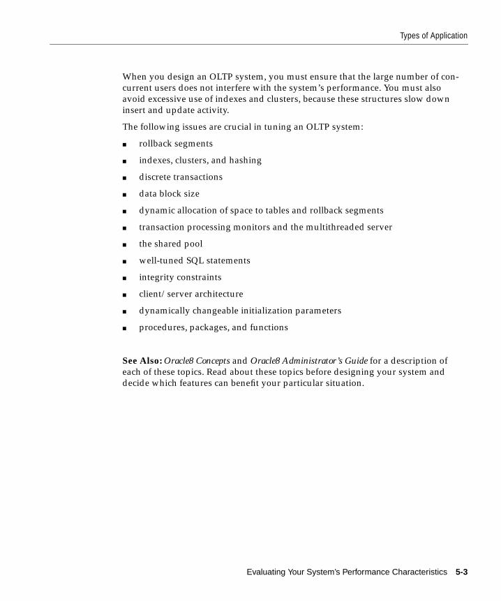
Types of Application
When you design an OLTP system, you must ensure that the large number of con-current users does not interfere with the system’s performance. You must alsoavoid excessive use of indexes and clusters, because these structures slow downinsert and update activity.
The following issues are crucial in tuning an OLTP system:
■ rollback segments
■ indexes, clusters, and hashing
■ discrete transactions
■ data block size
■ dynamic allocation of space to tables and rollback segments
■ transaction processing monitors and the multithreaded server
■ the shared pool
■ well-tuned SQL statements
■ integrity constraints
■ client/server architecture
■ dynamically changeable initialization parameters
■ procedures, packages, and functions
See Also: Oracle8 Concepts and Oracle8 Administrator’s Guide for a description ofeach of these topics. Read about these topics before designing your system anddecide which features can benefit your particular situation.
Evaluating Your System’s Performance Characteristics 5-3
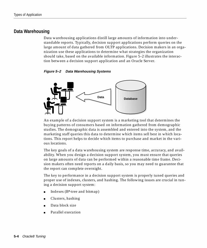
Types of Application
Data WarehousingData warehousing applications distill large amounts of information into under-standable reports. Typically, decision support applications perform queries on thelarge amount of data gathered from OLTP applications. Decision makers in an orga-nization use these applications to determine what strategies the organizationshould take, based on the available information. Figure 5–2 illustrates the interac-tion between a decision support application and an Oracle Server.
Figure 5–2 Data Warehousing Systems
An example of a decision support system is a marketing tool that determines thebuying patterns of consumers based on information gathered from demographicstudies. The demographic data is assembled and entered into the system, and themarketing staff queries this data to determine which items sell best in which loca-tions. This report helps to decide which items to purchase and market in the vari-ous locations.
The key goals of a data warehousing system are response time, accuracy, and avail-ability. When you design a decision support system, you must ensure that querieson large amounts of data can be performed within a reasonable time frame. Deci-sion makers often need reports on a daily basis, so you may need to guarantee thatthe report can complete overnight.
The key to performance in a decision support system is properly tuned queries andproper use of indexes, clusters, and hashing. The following issues are crucial in tun-ing a decision support system:
■ Indexes (B*-tree and bitmap)
■ Clusters, hashing
■ Data block size
■ Parallel execution
DatabaseData
5-4 Oracle8 Tuning
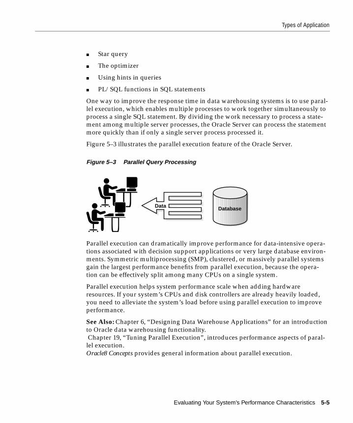
Types of Application
■ Star query
■ The optimizer
■ Using hints in queries
■ PL/SQL functions in SQL statements
One way to improve the response time in data warehousing systems is to use paral-lel execution, which enables multiple processes to work together simultaneously toprocess a single SQL statement. By dividing the work necessary to process a state-ment among multiple server processes, the Oracle Server can process the statementmore quickly than if only a single server process processed it.
Figure 5–3 illustrates the parallel execution feature of the Oracle Server.
Figure 5–3 Parallel Query Processing
Parallel execution can dramatically improve performance for data-intensive opera-tions associated with decision support applications or very large database environ-ments. Symmetric multiprocessing (SMP), clustered, or massively parallel systemsgain the largest performance benefits from parallel execution, because the opera-tion can be effectively split among many CPUs on a single system.
Parallel execution helps system performance scale when adding hardwareresources. If your system’s CPUs and disk controllers are already heavily loaded,you need to alleviate the system’s load before using parallel execution to improveperformance.
See Also: Chapter 6, “Designing Data Warehouse Applications” for an introductionto Oracle data warehousing functionality. Chapter 19, “Tuning Parallel Execution”, introduces performance aspects of paral-lel execution.Oracle8 Concepts provides general information about parallel execution.
DatabaseData
Evaluating Your System’s Performance Characteristics 5-5
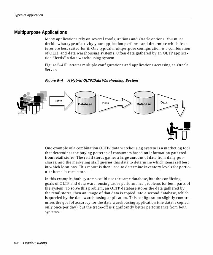
Types of Application
Multipurpose ApplicationsMany applications rely on several configurations and Oracle options. You mustdecide what type of activity your application performs and determine which fea-tures are best suited for it. One typical multipurpose configuration is a combinationof OLTP and data warehousing systems. Often data gathered by an OLTP applica-tion “feeds” a data warehousing system.
Figure 5–4 illustrates multiple configurations and applications accessing an OracleServer.
Figure 5–4 A Hybrid OLTP/Data Warehousing System
One example of a combination OLTP/data warehousing system is a marketing toolthat determines the buying patterns of consumers based on information gatheredfrom retail stores. The retail stores gather a large amount of data from daily pur-chases, and the marketing staff queries this data to determine which items sell bestin which locations. This report is then used to determine inventory levels for partic-ular items in each store.
In this example, both systems could use the same database, but the conflictinggoals of OLTP and data warehousing cause performance problems for both parts ofthe system. To solve this problem, an OLTP database stores the data gathered bythe retail stores, then an image of that data is copied into a second database, whichis queried by the data warehousing application. This configuration slightly compro-mises the goal of accuracy for the data warehousing application (the data is copiedonly once per day), but the trade-off is significantly better performance from bothsystems.
Database DataDataDataDatabase
5-6 Oracle8 Tuning
Oracle Configurations
For hybrid systems you must determine which goals are most important. You mayneed to compromise on meeting lower-priority goals to achieve acceptable perfor-mance across the whole system.
Oracle ConfigurationsYou can configure your system depending on the hardware and software availableto you. The basic configurations are:
■ Distributed Systems
■ The Oracle Parallel Server
■ Client/Server Configurations
Depending on your application and your operating system, each of these or a com-bination of these configurations will best suit your needs.
Distributed SystemsDistributed applications involve spreading data over multiple databases on multi-ple machines. Several smaller server machines can be cheaper and more flexiblethan one large, centrally located server. This configuration takes advantage ofsmall, powerful server machines and cheaper connectivity options. Distributed sys-tems allow you to have data physically located at several sites, and each site cantransparently access all of the data.
Figure 5–5 illustrates the distributed database configuration of the Oracle Server.
Evaluating Your System’s Performance Characteristics 5-7
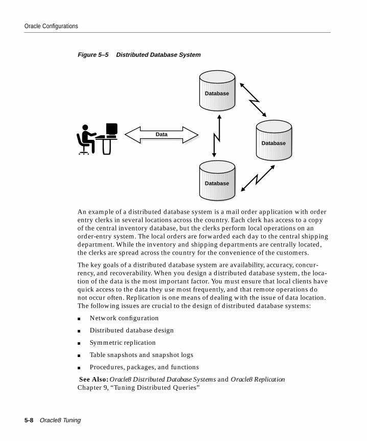
Oracle Configurations
Figure 5–5 Distributed Database System
An example of a distributed database system is a mail order application with orderentry clerks in several locations across the country. Each clerk has access to a copyof the central inventory database, but the clerks perform local operations on anorder-entry system. The local orders are forwarded each day to the central shippingdepartment. While the inventory and shipping departments are centrally located,the clerks are spread across the country for the convenience of the customers.
The key goals of a distributed database system are availability, accuracy, concur-rency, and recoverability. When you design a distributed database system, the loca-tion of the data is the most important factor. You must ensure that local clients havequick access to the data they use most frequently, and that remote operations donot occur often. Replication is one means of dealing with the issue of data location.The following issues are crucial to the design of distributed database systems:
■ Network configuration
■ Distributed database design
■ Symmetric replication
■ Table snapshots and snapshot logs
■ Procedures, packages, and functions
See Also: Oracle8 Distributed Database Systems and Oracle8 ReplicationChapter 9, “Tuning Distributed Queries”
Database
Database
Data
Database
5-8 Oracle8 Tuning
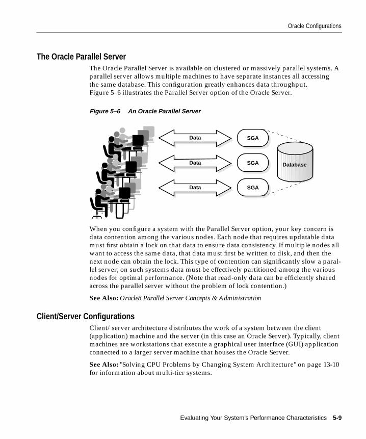
Oracle Configurations
The Oracle Parallel ServerThe Oracle Parallel Server is available on clustered or massively parallel systems. Aparallel server allows multiple machines to have separate instances all accessingthe same database. This configuration greatly enhances data throughput.Figure 5–6 illustrates the Parallel Server option of the Oracle Server.
Figure 5–6 An Oracle Parallel Server
When you configure a system with the Parallel Server option, your key concern isdata contention among the various nodes. Each node that requires updatable datamust first obtain a lock on that data to ensure data consistency. If multiple nodes allwant to access the same data, that data must first be written to disk, and then thenext node can obtain the lock. This type of contention can significantly slow a paral-lel server; on such systems data must be effectively partitioned among the variousnodes for optimal performance. (Note that read-only data can be efficiently sharedacross the parallel server without the problem of lock contention.)
See Also: Oracle8 Parallel Server Concepts & Administration
Client/Server ConfigurationsClient/server architecture distributes the work of a system between the client(application) machine and the server (in this case an Oracle Server). Typically, clientmachines are workstations that execute a graphical user interface (GUI) applicationconnected to a larger server machine that houses the Oracle Server.
See Also: "Solving CPU Problems by Changing System Architecture" on page 13-10for information about multi-tier systems.
Data Database
Data
Data
SGA
SGA
SGA
Evaluating Your System’s Performance Characteristics 5-9

Oracle Configurations
5-10 Oracle8 Tuning
Designing Data Warehouse Applica
6
Designing Data Warehouse ApplicationsThis chapter introduces integrated Oracle8 features for tuning enterprise-scale datawarehouses. By intelligently tuning the system, the data layout, and the applica-tion, you can build a high performance, scalable data warehouse.
Topics in this chapter include
■ Introduction
■ Features for Building a Data Warehouse
■ Features for Querying a Data Warehouse
■ Backup and Recovery of the Data Warehouse
tions 6-1
Introduction
IntroductionData warehousing applications process a substantial amount of data by means ofmany CPU- and I/O-bound, data-intensive tasks such as
■ loading, indexing, and summarizing tables
■ scanning, joining, sorting, aggregating, and fetching data
The resource required to complete the tasks on many gigabytes of data distin-guishes data warehousing applications from other types of data processing. Thebulk and complexity of your data may clearly indicate that you need to deploy mul-tiple CPUs, investigate parallel processing, or consider specific data processing fea-tures that are directly relevant to the tasks at hand.
For example, in a typical data warehousing application, data-intensive tasks mightbe performed on 100 gigabytes of data. At a processing speed of 0.2 G to 2 G ofdata per hour per CPU, a single CPU might need from 2 days to more than 2 weeksto perform a task. With more than a single gigabyte of data (certainly with upwardsof 10G), you need to consider increasing the number of CPUs.
Similarly, if you need to copy 10 gigabytes of data, consider that using Export/Import might take a single CPU 10 hours. By contrast, using parallel CREATETABLE . . . AS SELECT on 10 CPUs might take only 1 hour.
Actual processing time depends on many factors, such as the complexity of the que-ries, the processing speed to which a particular hardware configuration can betuned, and so on. Always run simple tests on your own system to find out its per-formance characteristics with regard to particular operations.
Features for Building a Data WarehouseThis section outlines Oracle8 features useful for building a data warehouse. Itincludes:
■ Parallel CREATE TABLE . . . AS SELECT
■ Parallel Index Creation
■ Fast Full Index Scan
■ Partitioned Tables
■ ANALYZE Command
■ Parallel Load
See Also: Oracle8 Concepts and Oracle8 SQL Reference
6-2 Oracle8 Tuning
Features for Building a Data Warehouse
Parallel CREATE TABLE . . . AS SELECTThe ability to CREATE TABLE . . . AS SELECT in parallel enables you to reorganizeextremely large tables efficiently. You might find it prohibitive to take a serialapproach to reorganizing or reclaiming space in a table containing tens or thou-sands of gigabytes of data. Using Export/Import to perform such a task mightresult in an unacceptable amount of downtime. If you have a lot of temporaryspace available, you can use CREATE TABLE . . . AS SELECT to perform such tasksin parallel. With this approach, redefining integrity constraints is optional. This fea-ture is often used for creating summary tables, which are precomputed resultsstored in the data warehouse.
See Also: "Creating and Populating Tables in Parallel" on page 19-51Oracle8 Concepts
Parallel Index CreationThe ability to create indexes in parallel benefits both data warehousing and OLTPapplications. On extremely large tables, rebuilding an index may take a long time.Periodically DBAs may load a large amount of data and rebuild the index. With theability to create indexes in parallel, you may be able to drop an index before load-ing new data, and re-create it afterward.
See Also: "Creating Indexes in Parallel" on page 19-53Chapter 19, “Tuning Parallel Execution”
Fast Full Index ScanFAST FULL SCAN on the index is a faster alternative to a full table scan when anexisting index already contains all the columns that are needed for the query. It canuse multiblock I/O and can be parallelized just like a table scan. The hintINDEX_FFS enforces fast full index scan.
See Also: "Fast Full Index Scan" on page 10-9"INDEX_FFS" on page 8-22
Designing Data Warehouse Applications 6-3
Features for Building a Data Warehouse
Partitioned TablesYou can avoid downtime with very large or mission-critical tables by using parti-tions. You can divide a large table into multiple physical tables using partitioningcriteria. In a data warehouse you can manage historical data by partitioning bydate. You can then perform on a partition level all of the operations you might nor-mally perform on the table level, such as backup and restore. You can add space fornew data by adding a new partition, and delete old data by dropping an existingpartition. Queries that use a key range to select from a partitioned table retrieveonly the partitions that fall within that range. In this way partitions offer significantimprovements in availability, administration and table scan performance.
Note: For performance reasons, in Oracle8 partitioned tables should be used ratherthan partition views. Please see Oracle8 Migration for instructions on migratingfrom partition views to partitioned tables.
See Also: Oracle8 Concepts for information about partitioned tables"Partitioning Data" on page 19-23
ANALYZE CommandYou can use the ANALYZE command to analyze the storage characteristics oftables, indexes, and clusters to gather statistics which are then stored in the datadictionary. The optimizer uses these statistics in a cost-based approach to deter-mine the most efficient execution plan for the SQL statements you issue. Note thatstatistics can be either computed or estimated, depending on the amount of over-head you are willing to allow for this purpose.
See Also: "Step 3: Analyzing Data" on page 19-36Oracle8 Administrator’s Guide
Parallel LoadWhen very large amounts of data must be loaded, the destination table may beunavailable for an unacceptable amount of time. The ability to load data in parallelcan dramatically slash the amount of downtime necessary.
See Also: Chapter 19, “Tuning Parallel Execution”, especially "Using Parallel Load"on page 19-25Oracle8 Utilities for a description of SQL Loader conventional and direct path loads.
6-4 Oracle8 Tuning
Features for Querying a Data Warehouse
Features for Querying a Data WarehouseThis section summarizes Oracle8 features useful for querying a data warehouse. Itincludes:
■ Oracle Parallel Server Option
■ Parallel-Aware Optimizer
■ Parallel Execution
■ Bitmap Indexes
■ Star Queries
■ Star Transformation
Oracle Parallel Server OptionThe Oracle Parallel Server option provides benefits important to both OLTP anddata warehousing applications:
■ application failover
■ scalable performance
■ load balancing
■ multiuser scalability
Oracle Parallel Server failover capability (the ability of the application to reconnectautomatically if the connection to the database is broken) results in improved avail-ability, a primary benefit for OLTP applications. Likewise, scalability in the numberof users that can connect to the database is a major benefit in OLTP environments.OLTP performance on Oracle Parallel Server can scale as well, if an application’sdata is isolated onto a single server.
For data warehousing applications, scalability of performance is a primary benefitof Oracle Parallel Server. The architecture of Oracle Parallel Server allows parallelquery to perform excellent load balancing of work at runtime. If a node in an Ora-cle Parallel Server cluster or MPP is temporarily slowed down, work that was origi-nally assigned to parallel query servers on that node (but not yet commenced bythose servers) may be performed by servers on other nodes, hence preventing thatnode from becoming a serious bottleneck. Even though Oracle Parallel Server is acornerstone of parallel query on clusters and MPPs, in a mostly query environmentthe overhead on the distributed lock manager is minimal.
See Also: Oracle8 Parallel Server Concepts & Administration
Designing Data Warehouse Applications 6-5
Features for Querying a Data Warehouse
Parallel-Aware OptimizerKnowledge about parallelism is incorporated into the Oracle8 cost-based optimizer.Parallel execution considerations are thus a fundamental component in arriving atquery execution plans. In addition, you can control the trade-off of throughput forresponse time in plan selection.
The optimizer chooses intelligent defaults for the degree of parallelism based onavailable processors and the number of disk drives storing data the query willaccess. Access path choices (such as table scans vs. index access) take into accountthe degree of parallelism, resulting in plans that are optimized for parallel execu-tion. Execution plans are more scalable, and there is improved correlation betweenoptimizer cost and execution time for parallel query.
The initialization parameter OPTIMIZER_PERCENT_PARALLEL defines theweighting that the optimizer uses to minimize response time in its cost functions.
See Also: "OPTIMIZER_PERCENT_PARALLEL" on page 19-4
Parallel ExecutionThe Oracle8 provides for improved performance through use of parallel execution.
Parallel execution enables multiple processes to work together simultaneously toprocess a single query or DML statement. By dividing the task among multipleserver processes, Oracle can execute the operation more quickly than if only oneserver process were used.
Parallel execution can dramatically improve performance for data-intensive datawarehousing operations. It helps systems scale in performance when adding hard-ware resources. The greatest performance benefits are on symmetric multiprocess-ing (SMP), clustered, or massively parallel systems where query processing can beeffectively spread out among many CPUs on a single system.
See Also: Chapter 19, “Tuning Parallel Execution”Oracle8 Concepts for conceptual background on parallel execution.
6-6 Oracle8 Tuning
Features for Querying a Data Warehouse
Bitmap IndexesRegular B*-tree indexes work best when each key or key range references only afew records, such as employee names. Bitmap indexes, by contrast, work best wheneach key references many records, such as employee gender.
Bitmap indexing provides the same functionality as regular indexes, but uses a dif-ferent internal representation, which makes it very fast and space efficient. Bitmapindexing benefits data warehousing applications that have large amounts of dataand ad hoc queries, but a low level of concurrent transactions. It provides reducedresponse time for many kinds of ad hoc queries; considerably reduced space usagecompared to other indexing techniques; and dramatic performance gains even onvery low end hardware. Bitmap indexes can be created in parallel and are com-pletely integrated with cost-based optimization.
See Also: "Using Bitmap Indexes" on page 10-13
Star QueriesOne type of data warehouse design is known as a “star” schema. This typically con-sists of one or more very large “fact” tables and a number of much smaller “dimen-sion” or reference tables. A star query is one that joins several of the dimensiontables, usually by predicates in the query, to one of the fact tables.
Oracle cost-based optimization recognizes star queries and generates efficient exe-cution plans for them; indeed, you must use cost-based optimization to get efficientstar query execution. To enable cost-based optimization, simply ANALYZE yourtables and be sure that the OPTIMIZER_MODE initialization parameter is set to itsdefault value of CHOOSE.
See Also: Oracle8 Concepts regarding optimization of star queries"STAR" on page 8-24 for information about the STAR hint
Designing Data Warehouse Applications 6-7
Backup and Recovery of the Data Warehouse
Star TransformationStar transformation is a cost-based transformation designed to execute star queriesefficiently. Whereas star optimization works well for schemas with a small numberof dimensions and dense fact tables, star transformation works well for schemaswith a large number of dimensions and sparse fact tables.
Star transformation is enabled by setting the initialization parameterSTAR_TRANSFORMATION_ENABLED to TRUE. You can use theSTAR_TRANSFORMATION hint to make the optimizer use the best plan in whichthe transformation has been used.
See Also: Oracle8 Concepts for a full discussion of star transformation.Oracle8 Reference describes the STAR_TRANSFORMATION_ENABLED initializa-tion parameter."STAR_TRANSFORMATION" on page 8-35 explains how to use this hint.
Backup and Recovery of the Data WarehouseRecoverability has various levels: recovery from disk failure, human error, softwarefailure, fire, and so on, requires different procedures. Oracle8 provides only part ofthe solution. Organizations must decide how much to spend on backup and recov-ery by considering the business cost of a long outage.
The NOLOGGING option enables you to perform certain operations without theoverhead of generating a log. Even without logging, you can avoid disk failure ifyou use disk mirroring or RAID technology. If you load your warehouse from tapesevery day or week, you might satisfactorily recover from all failures simply by sav-ing copies of the tape in several remote locations and reloading from tape whensomething goes wrong.
At the other end of the spectrum, you could both mirror disks and take backupsand archive logs, and maintain a remote standby system. The mirrored disks pre-vent loss of availability for disk failure, and also protect against total loss in theevent of human error (such as dropping the wrong table) or software error (such asdisk block corruption). In the event of fire, power failure, or other problems at theprimary site, the backup site prevents long outages.
See Also: For more information on recovery and the NOLOGGING option, see theOracle8 Administrator’s Guide and Oracle8 SQL Reference."[NO]LOGGING Option" on page 19-35
6-8 Oracle8 Tuning
Part III
Optimizing Database OperationsPart 3 discusses how to tune your database and the various methods you use toaccess data for optimal database performance. The chapters in Part 3 are:
■ Chapter 7, “Tuning Database Operations”
■ Chapter 8, “Optimization Modes and Hints”
■ Chapter 9, “Tuning Distributed Queries”
■ Chapter 10, “Data Access Methods”
■ Chapter 11, “Oracle8 Transaction Modes”
■ Chapter 12, “Managing SQL and Shared PL/SQL Areas”

Tuning Database Opera
7
Tuning Database OperationsStructured Query Language (SQL) is used to perform all database operations,although some Oracle tools and applications simplify or mask its use. This chapterprovides an overview of the issues involved in tuning database operations:
■ Tuning Goals
■ Methodology for Tuning Database Operations
■ Approaches to SQL Statement Tuning
tions 7-1
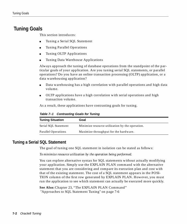
Tuning Goals
Tuning GoalsThis section introduces:
■ Tuning a Serial SQL Statement
■ Tuning Parallel Operations
■ Tuning OLTP Applications
■ Tuning Data Warehouse Applications
Always approach the tuning of database operations from the standpoint of the par-ticular goals of your application. Are you tuning serial SQL statements, or paralleloperations? Do you have an online transaction processing (OLTP) application, or adata warehousing application?
■ Data warehousing has a high correlation with parallel operations and high datavolume.
■ OLTP applications have a high correlation with serial operations and hightransaction volume.
As a result, these applications have contrasting goals for tuning.
Tuning a Serial SQL StatementThe goal of tuning one SQL statement in isolation can be stated as follows:
To minimize resource utilization by the operation being performed.
You can explore alternative syntax for SQL statements without actually modifyingyour application. Simply use the EXPLAIN PLAN command with the alternativestatement that you are considering and compare its execution plan and cost withthat of the existing statement. The cost of a SQL statement appears in the POSI-TION column of the first row generated by EXPLAIN PLAN. However, you mustrun the application to see which statement can actually be executed more quickly.
See Also: Chapter 23, “The EXPLAIN PLAN Command” "Approaches to SQL Statement Tuning" on page 7-6
Table 7–1 Contrasting Goals for Tuning
Tuning Situation Goal
Serial SQL Statement Minimize resource utilization by the operation.
Parallel Operations Maximize throughput for the hardware.
7-2 Oracle8 Tuning
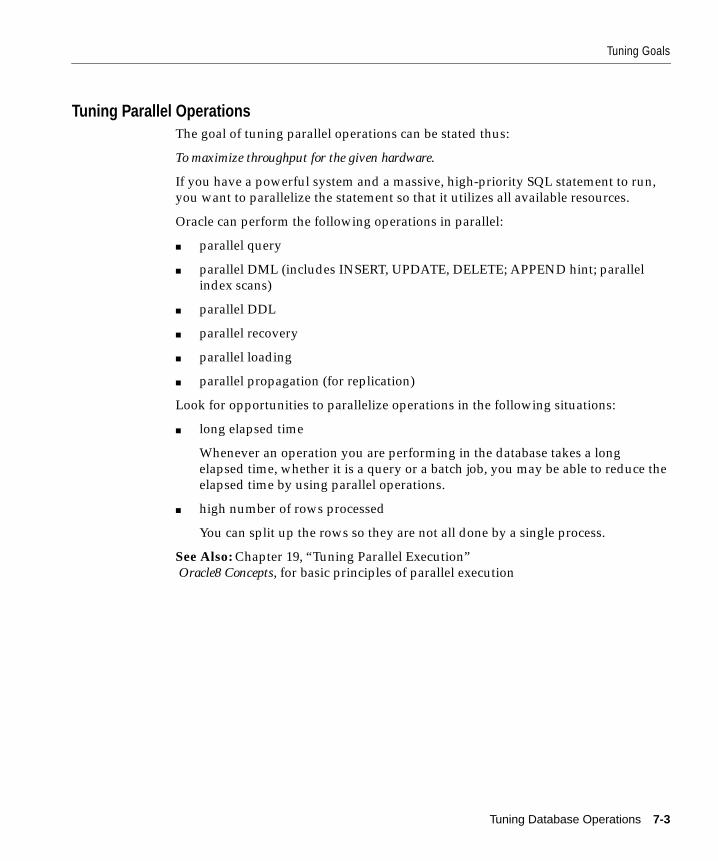
Tuning Goals
Tuning Parallel OperationsThe goal of tuning parallel operations can be stated thus:
To maximize throughput for the given hardware.
If you have a powerful system and a massive, high-priority SQL statement to run,you want to parallelize the statement so that it utilizes all available resources.
Oracle can perform the following operations in parallel:
■ parallel query
■ parallel DML (includes INSERT, UPDATE, DELETE; APPEND hint; parallelindex scans)
■ parallel DDL
■ parallel recovery
■ parallel loading
■ parallel propagation (for replication)
Look for opportunities to parallelize operations in the following situations:
■ long elapsed time
Whenever an operation you are performing in the database takes a longelapsed time, whether it is a query or a batch job, you may be able to reduce theelapsed time by using parallel operations.
■ high number of rows processed
You can split up the rows so they are not all done by a single process.
See Also: Chapter 19, “Tuning Parallel Execution” Oracle8 Concepts, for basic principles of parallel execution
Tuning Database Operations 7-3
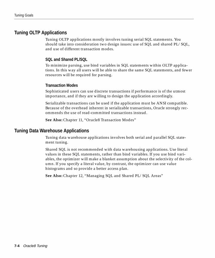
Tuning Goals
Tuning OLTP ApplicationsTuning OLTP applications mostly involves tuning serial SQL statements. Youshould take into consideration two design issues: use of SQL and shared PL/SQL,and use of different transaction modes.
SQL and Shared PL/SQLTo minimize parsing, use bind variables in SQL statements within OLTP applica-tions. In this way all users will be able to share the same SQL statements, and fewerresources will be required for parsing.
Transaction ModesSophisticated users can use discrete transactions if performance is of the utmostimportance, and if they are willing to design the application accordingly.
Serializable transactions can be used if the application must be ANSI compatible.Because of the overhead inherent in serializable transactions, Oracle strongly rec-ommends the use of read-committed transactions instead.
See Also: Chapter 11, “Oracle8 Transaction Modes”
Tuning Data Warehouse ApplicationsTuning data warehouse applications involves both serial and parallel SQL state-ment tuning.
Shared SQL is not recommended with data warehousing applications. Use literalvalues in these SQL statements, rather than bind variables. If you use bind vari-ables, the optimizer will make a blanket assumption about the selectivity of the col-umn. If you specify a literal value, by contrast, the optimizer can use valuehistograms and so provide a better access plan.
See Also: Chapter 12, “Managing SQL and Shared PL/SQL Areas”
7-4 Oracle8 Tuning
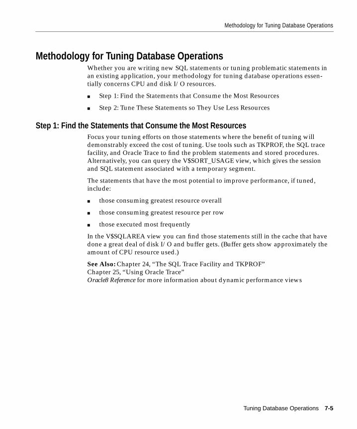
Methodology for Tuning Database Operations
Methodology for Tuning Database OperationsWhether you are writing new SQL statements or tuning problematic statements inan existing application, your methodology for tuning database operations essen-tially concerns CPU and disk I/O resources.
■ Step 1: Find the Statements that Consume the Most Resources
■ Step 2: Tune These Statements so They Use Less Resources
Step 1: Find the Statements that Consume the Most ResourcesFocus your tuning efforts on those statements where the benefit of tuning willdemonstrably exceed the cost of tuning. Use tools such as TKPROF, the SQL tracefacility, and Oracle Trace to find the problem statements and stored procedures.Alternatively, you can query the V$SORT_USAGE view, which gives the sessionand SQL statement associated with a temporary segment.
The statements that have the most potential to improve performance, if tuned,include:
■ those consuming greatest resource overall
■ those consuming greatest resource per row
■ those executed most frequently
In the V$SQLAREA view you can find those statements still in the cache that havedone a great deal of disk I/O and buffer gets. (Buffer gets show approximately theamount of CPU resource used.)
See Also: Chapter 24, “The SQL Trace Facility and TKPROF”Chapter 25, “Using Oracle Trace”Oracle8 Reference for more information about dynamic performance views
Tuning Database Operations 7-5
Approaches to SQL Statement Tuning
Step 2: Tune These Statements so They Use Less ResourcesRemember that application design is fundamental to performance. No amount ofSQL statement tuning can make up for inefficient design. If you encounter stum-bling blocks in SQL statement tuning, perhaps you need to change the applicationdesign.
You can use two strategies to reduce the resources consumed by a particular state-ment:
■ Get the statement to use less resources when it is used.
■ Use the statement less frequently.
Statements may use the most resources because they do the most work, or becausethey perform their work inefficiently—or they may do both. However, the lowerthe resource used per unit of work (per row processed), the more likely it is thatyou can significantly reduce resources used only by changing the application itself.That is, rather than changing the SQL, it may be more effective to have the applica-tion process fewer rows, or process the same rows less frequently.
These two approaches are not mutually exclusive. The former is clearly less expen-sive, because you should be able to accomplish it either without program change(by changing index structures) or by changing only the SQL statement itself ratherthan the surrounding logic.
See Also: Chapter 13, “Tuning CPU Resources”Chapter 15, “Tuning I/O”
Approaches to SQL Statement TuningThis section describes three strategies you can use to speed up SQL statements:
■ Restructure the Indexes
■ Restructure the Statement
■ Restructure the Data
Note: These guidelines are oriented to production SQL that will be executed fre-quently. Most of the techniques that are discouraged here can legitimately beemployed in ad hoc statements or in applications run infrequently, where perfor-mance is not critical.
7-6 Oracle8 Tuning
Approaches to SQL Statement Tuning
Restructure the IndexesRestructuring the indexes is a good starting point, because it has more impact onthe application than does restructuring the statement or the data.
■ Remove nonselective indexes to speed the DML.
■ Index performance-critical access paths.
■ Consider hash clusters, but watch uniqueness.
■ Consider index clusters only if the cluster keys are similarly sized.
Do not use indexes as a panacea. Application developers sometimes think that per-formance will improve if they just write enough indexes. If a single programmercreates an appropriate index, this might indeed improve the application’s perfor-mance. However, if 50 programmers each create an index, application performancewill probably be hampered!
Restructure the StatementAfter restructuring the indexes, you can try restructuring the statement. Rewritingan inefficient SQL statement is often easier than repairing it. If you understand thepurpose of a given statement, you may be able to quickly and easily write a newstatement that meets the requirement.
Consider Alternative SQL SyntaxBecause SQL is a flexible language, more than one SQL statement may meet theneeds of your application. Although two SQL statements may produce the sameresult, Oracle may process one faster than the other. You can use the results of theEXPLAIN PLAN statement to compare the execution plans and costs of the twostatements and determine which is more efficient.
This example shows the execution plans for two SQL statements that perform thesame function. Both statements return all the departments in the DEPT table thathave no employees in the EMP table. Each statement searches the EMP table with asubquery. Assume there is an index, DEPTNO_INDEX, on the DEPTNO column ofthe EMP table.
This is the first statement and its execution plan:
SELECT dname, deptno FROM dept WHERE deptno NOT IN (SELECT deptno FROM emp);
Tuning Database Operations 7-7
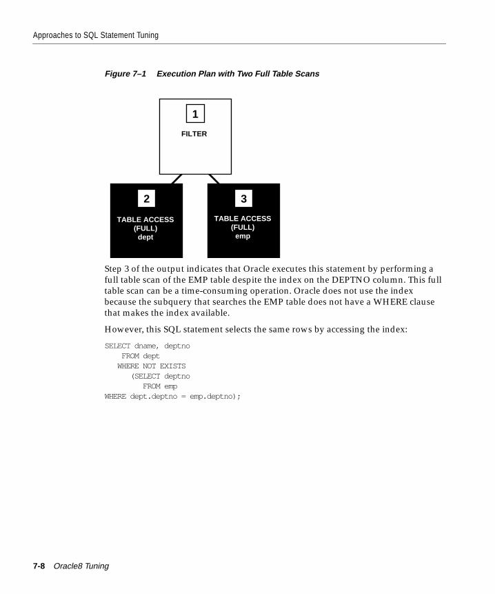
Approaches to SQL Statement Tuning
Figure 7–1 Execution Plan with Two Full Table Scans
Step 3 of the output indicates that Oracle executes this statement by performing afull table scan of the EMP table despite the index on the DEPTNO column. This fulltable scan can be a time-consuming operation. Oracle does not use the indexbecause the subquery that searches the EMP table does not have a WHERE clausethat makes the index available.
However, this SQL statement selects the same rows by accessing the index:
SELECT dname, deptno FROM dept WHERE NOT EXISTS (SELECT deptno FROM empWHERE dept.deptno = emp.deptno);
TABLE ACCESS(FULL)
dept
2 3
TABLE ACCESS(FULL)
emp
1
FILTER
7-8 Oracle8 Tuning
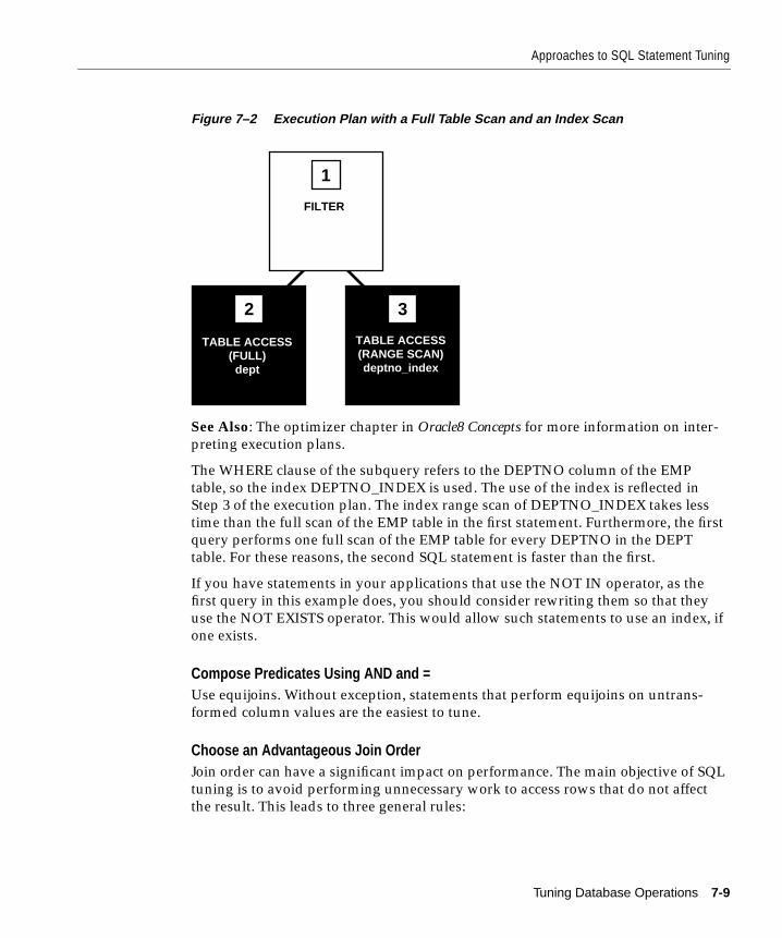
Approaches to SQL Statement Tuning
Figure 7–2 Execution Plan with a Full Table Scan and an Index Scan
See Also: The optimizer chapter in Oracle8 Concepts for more information on inter-preting execution plans.
The WHERE clause of the subquery refers to the DEPTNO column of the EMPtable, so the index DEPTNO_INDEX is used. The use of the index is reflected inStep 3 of the execution plan. The index range scan of DEPTNO_INDEX takes lesstime than the full scan of the EMP table in the first statement. Furthermore, the firstquery performs one full scan of the EMP table for every DEPTNO in the DEPTtable. For these reasons, the second SQL statement is faster than the first.
If you have statements in your applications that use the NOT IN operator, as thefirst query in this example does, you should consider rewriting them so that theyuse the NOT EXISTS operator. This would allow such statements to use an index, ifone exists.
Compose Predicates Using AND and =Use equijoins. Without exception, statements that perform equijoins on untrans-formed column values are the easiest to tune.
Choose an Advantageous Join OrderJoin order can have a significant impact on performance. The main objective of SQLtuning is to avoid performing unnecessary work to access rows that do not affectthe result. This leads to three general rules:
TABLE ACCESS(FULL)
dept
2 3
TABLE ACCESS(RANGE SCAN)deptno_index
1
FILTER
Tuning Database Operations 7-9
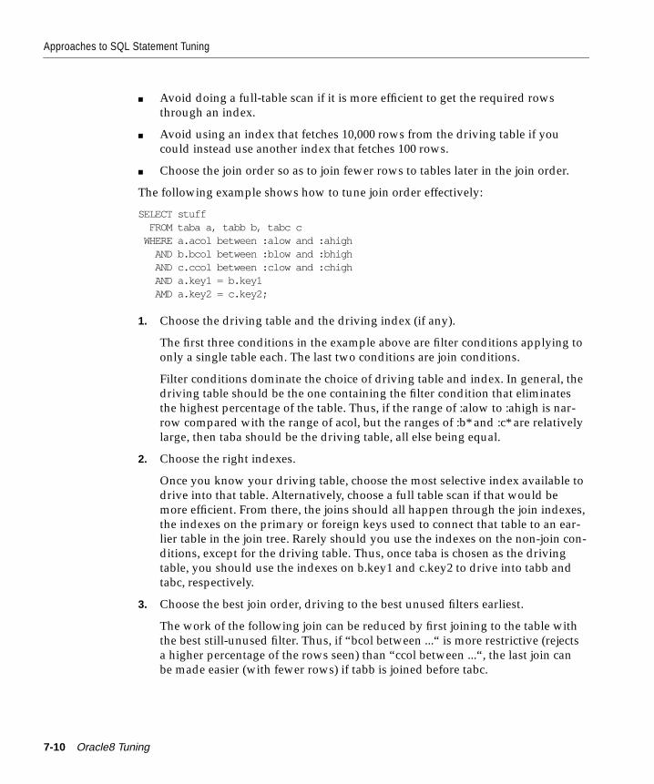
Approaches to SQL Statement Tuning
■ Avoid doing a full-table scan if it is more efficient to get the required rowsthrough an index.
■ Avoid using an index that fetches 10,000 rows from the driving table if youcould instead use another index that fetches 100 rows.
■ Choose the join order so as to join fewer rows to tables later in the join order.
The following example shows how to tune join order effectively:
SELECT stuff FROM taba a, tabb b, tabc c WHERE a.acol between :alow and :ahigh AND b.bcol between :blow and :bhigh AND c.ccol between :clow and :chigh AND a.key1 = b.key1 AMD a.key2 = c.key2;
1. Choose the driving table and the driving index (if any).
The first three conditions in the example above are filter conditions applying toonly a single table each. The last two conditions are join conditions.
Filter conditions dominate the choice of driving table and index. In general, thedriving table should be the one containing the filter condition that eliminatesthe highest percentage of the table. Thus, if the range of :alow to :ahigh is nar-row compared with the range of acol, but the ranges of :b* and :c* are relativelylarge, then taba should be the driving table, all else being equal.
2. Choose the right indexes.
Once you know your driving table, choose the most selective index available todrive into that table. Alternatively, choose a full table scan if that would bemore efficient. From there, the joins should all happen through the join indexes,the indexes on the primary or foreign keys used to connect that table to an ear-lier table in the join tree. Rarely should you use the indexes on the non-join con-ditions, except for the driving table. Thus, once taba is chosen as the drivingtable, you should use the indexes on b.key1 and c.key2 to drive into tabb andtabc, respectively.
3. Choose the best join order, driving to the best unused filters earliest.
The work of the following join can be reduced by first joining to the table withthe best still-unused filter. Thus, if “bcol between ...“ is more restrictive (rejectsa higher percentage of the rows seen) than “ccol between ...“, the last join canbe made easier (with fewer rows) if tabb is joined before tabc.
7-10 Oracle8 Tuning
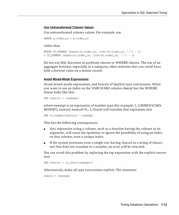
Approaches to SQL Statement Tuning
Use Untransformed Column ValuesUse untransformed column values. For example, use
WHERE a.order_no = b.order_no
rather than
WHERE TO_NUMBER (substr(a.order_no, instr(b.order_no, ’.’) - 1)= TO_NUMBER (substr(a.order_no, instr(b.order_no, ’.’) - 1)
Do not use SQL functions in predicate clauses or WHERE clauses. The use of anaggregate function, especially in a subquery, often indicates that you could haveheld a derived value on a master record.
Avoid Mixed-Mode ExpressionsAvoid mixed-mode expressions, and beware of implicit type conversions. Whenyou want to use an index on the VARCHAR2 column charcol, but the WHEREclause looks like this:
AND charcol = <numexpr>
where numexpr is an expression of number type (for example, 1, USERENV('SES-SIONID'), numcol, numcol+0,...), Oracle will translate that expression into
AND to_number(charcol) = numexpr
This has the following consequences:
■ Any expression using a column, such as a function having the column as itsargument, will cause the optimizer to ignore the possibility of using an indexon that column, even a unique index.
■ If the system processes even a single row having charcol as a string of charac-ters that does not translate to a number, an error will be returned.
You can avoid this problem by replacing the top expression with the explicit conver-sion
AND charcol = to_char(<numexpr>)
Alternatively, make all type conversions explicit. The statement
numcol = charexpr
Tuning Database Operations 7-11
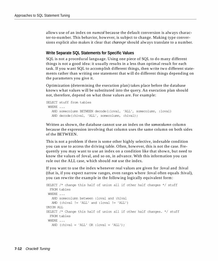
Approaches to SQL Statement Tuning
allows use of an index on numcol because the default conversion is always charac-ter-to-number. This behavior, however, is subject to change. Making type conver-sions explicit also makes it clear that charexpr should always translate to a number.
Write Separate SQL Statements for Specific ValuesSQL is not a procedural language. Using one piece of SQL to do many differentthings is not a good idea: it usually results in a less than optimal result for eachtask. If you want SQL to accomplish different things, then write two different state-ments rather than writing one statement that will do different things depending onthe parameters you give it.
Optimization (determining the execution plan) takes place before the databaseknows what values will be substituted into the query. An execution plan shouldnot, therefore, depend on what those values are. For example:
SELECT stuff from tables WHERE ... AND somecolumn BETWEEN decode(:loval, 'ALL', somecolumn, :loval) AND decode(:hival, 'ALL', somecolumn, :hival);
Written as shown, the database cannot use an index on the somecolumn columnbecause the expression involving that column uses the same column on both sidesof the BETWEEN.
This is not a problem if there is some other highly selective, indexable conditionyou can use to access the driving table. Often, however, this is not the case. Fre-quently you may want to use an index on a condition like that shown, but need toknow the values of :loval, and so on, in advance. With this information you canrule out the ALL case, which should not use the index.
If you want to use the index whenever real values are given for :loval and :hival(that is, if you expect narrow ranges, even ranges where :loval often equals :hival),you can rewrite the example in the following logically equivalent form:
SELECT /* change this half of union all if other half changes */ stuff FROM tables WHERE ... AND somecolumn between :loval and :hival AMD (:hival != 'ALL' and :loval != 'ALL')UNION ALLSELECT /* Change this half of union all if other half changes. */ stuff FROM tables WHERE ... AND (:hival = 'ALL' OR :loval = 'ALL');
7-12 Oracle8 Tuning
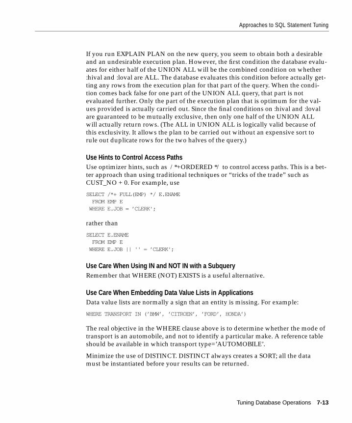
Approaches to SQL Statement Tuning
If you run EXPLAIN PLAN on the new query, you seem to obtain both a desirableand an undesirable execution plan. However, the first condition the database evalu-ates for either half of the UNION ALL will be the combined condition on whether:hival and :loval are ALL. The database evaluates this condition before actually get-ting any rows from the execution plan for that part of the query. When the condi-tion comes back false for one part of the UNION ALL query, that part is notevaluated further. Only the part of the execution plan that is optimum for the val-ues provided is actually carried out. Since the final conditions on :hival and :lovalare guaranteed to be mutually exclusive, then only one half of the UNION ALLwill actually return rows. (The ALL in UNION ALL is logically valid because ofthis exclusivity. It allows the plan to be carried out without an expensive sort torule out duplicate rows for the two halves of the query.)
Use Hints to Control Access PathsUse optimizer hints, such as /*+ORDERED */ to control access paths. This is a bet-ter approach than using traditional techniques or “tricks of the trade” such asCUST_NO + 0. For example, use
SELECT /*+ FULL(EMP) */ E.ENAME FROM EMP E WHERE E.JOB = ’CLERK';
rather than
SELECT E.ENAME FROM EMP E WHERE E.JOB || '' = ’CLERK';
Use Care When Using IN and NOT IN with a SubqueryRemember that WHERE (NOT) EXISTS is a useful alternative.
Use Care When Embedding Data Value Lists in ApplicationsData value lists are normally a sign that an entity is missing. For example:
WHERE TRANSPORT IN (’BMW’, ’CITROEN’, ’FORD’, HONDA’)
The real objective in the WHERE clause above is to determine whether the mode oftransport is an automobile, and not to identify a particular make. A reference tableshould be available in which transport type=’AUTOMOBILE’.
Minimize the use of DISTINCT. DISTINCT always creates a SORT; all the datamust be instantiated before your results can be returned.
Tuning Database Operations 7-13
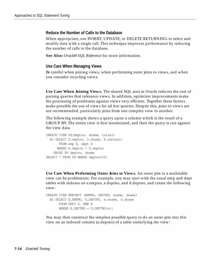
Approaches to SQL Statement Tuning
Reduce the Number of Calls to the DatabaseWhen appropriate, use INSERT, UPDATE, or DELETE RETURNING to select andmodify data with a single call. This technique improves performance by reducingthe number of calls to the database.
See Also: Oracle8 SQL Reference for more information.
Use Care When Managing ViewsBe careful when joining views, when performing outer joins to views, and whenyou consider recycling views.
Use Care When Joining Views. The shared SQL area in Oracle reduces the cost ofparsing queries that reference views. In addition, optimizer improvements makethe processing of predicates against views very efficient. Together these factorsmake possible the use of views for ad hoc queries. Despite this, joins to views arenot recommended, particularly joins from one complex view to another.
The following example shows a query upon a column which is the result of aGROUP BY. The entire view is first instantiated, and then the query is run againstthe view data.
CREATE VIEW DX(deptno, dname, totsal) AS SELECT D.deptno, D.dname, E.sum(sal) FROM emp E, dept D WHERE E.deptno = D.deptno GROUP BY deptno, dnameSELECT * FROM DX WHERE deptno=10;
Use Care When Performing Outer Joins to Views. An outer join to a multitableview can be problematic. For example, you may start with the usual emp and depttables with indexes on e.empno, e.deptno, and d.deptno, and create the followingview:
CREATE VIEW EMPDEPT (EMPNO, DEPTNO, ename, dname) AS SELECT E.EMPNO, E.DEPTNO, e.ename, d.dname FROM DEPT D, EMP E WHERE E.DEPTNO = D.DEPTNO(+);
You may then construct the simplest possible query to do an outer join into thisview on an indexed column (e.deptno) of a table underlying the view:
7-14 Oracle8 Tuning
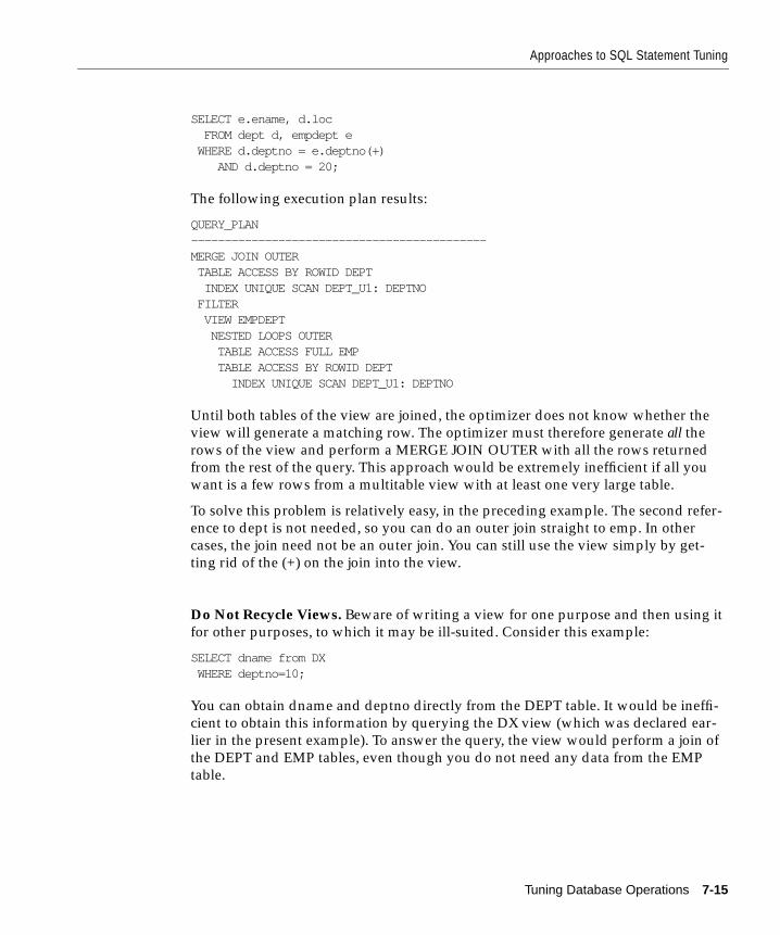
Approaches to SQL Statement Tuning
SELECT e.ename, d.loc FROM dept d, empdept e WHERE d.deptno = e.deptno(+) AND d.deptno = 20;
The following execution plan results:
QUERY_PLAN--------------------------------------------MERGE JOIN OUTER TABLE ACCESS BY ROWID DEPT INDEX UNIQUE SCAN DEPT_U1: DEPTNO FILTER VIEW EMPDEPT NESTED LOOPS OUTER TABLE ACCESS FULL EMP TABLE ACCESS BY ROWID DEPT INDEX UNIQUE SCAN DEPT_U1: DEPTNO
Until both tables of the view are joined, the optimizer does not know whether theview will generate a matching row. The optimizer must therefore generate all therows of the view and perform a MERGE JOIN OUTER with all the rows returnedfrom the rest of the query. This approach would be extremely inefficient if all youwant is a few rows from a multitable view with at least one very large table.
To solve this problem is relatively easy, in the preceding example. The second refer-ence to dept is not needed, so you can do an outer join straight to emp. In othercases, the join need not be an outer join. You can still use the view simply by get-ting rid of the (+) on the join into the view.
Do Not Recycle Views. Beware of writing a view for one purpose and then using itfor other purposes, to which it may be ill-suited. Consider this example:
SELECT dname from DX WHERE deptno=10;
You can obtain dname and deptno directly from the DEPT table. It would be ineffi-cient to obtain this information by querying the DX view (which was declared ear-lier in the present example). To answer the query, the view would perform a join ofthe DEPT and EMP tables, even though you do not need any data from the EMPtable.
Tuning Database Operations 7-15
Approaches to SQL Statement Tuning
Restructure the DataAfter restructuring the indexes and the statement, you can consider restructuringthe data.
■ Introduce derived values. Avoid GROUP BY in response-critical code.
■ Implement missing entities and intersection tables.
■ Reduce the network load. Migrate, replicate, partition data.
The overall purpose of any strategy for data distribution is to locate each dataattribute such that its value makes the minimum number of network journeys. Ifthe current number of journeys is excessive, then moving (migrating) the data is anatural solution.
Often, however, no single location of the data reduces the network load (or mes-sage transmission delays) to an acceptable level. In this case, consider either hold-ing multiple copies (replicating the data) or holding different parts of the data indifferent places (partitioning the data).
Where distributed queries are necessary, it may be effective to code the requiredjoins procedurally either in PL/SQL within a stored procedure, or within the userinterface code.
When considering a cross-network join, note that you can either bring the data infrom a remote node and perform the join locally, or you can perform the joinremotely. The option you choose should be determined by the relative volume ofdata on the different nodes.
7-16 Oracle8 Tuning
Optimization Modes and
8
Optimization Modes and HintsThis chapter explains when to use the available optimization modes and how touse hints to enhance Oracle performance.
Topics include:
■ Using Cost-Based Optimization
■ Using Rule-Based Optimization
■ Introduction to Hints
■ How to Specify Hints
■ Hints for Optimization Approaches and Goals
■ Hints for Access Methods
■ Hints for Join Orders
■ Hints for Join Operations
■ Hints for Parallel Execution
■ Additional Hints
■ Using Hints with Views
See Also: Oracle8 Concepts for an introduction to the optimizer, access methods, joinoperations, and parallel execution.
Hints 8-1
Using Cost-Based Optimization
Using Cost-Based OptimizationThis section discusses:
■ When to Use the Cost-Based Approach
■ How to Use the Cost-Based Approach
■ Using Histograms for Nonuniformly Distributed Data
■ Generating Statistics
■ Choosing a Goal for the Cost-Based Approach
■ Parameters that Affect Cost-Based Optimization Plans
■ Tips for Using the Cost-Based Approach
When to Use the Cost-Based ApproachAttention: In general, you should always use the cost-based optimizationapproach. The rule-based approach is available for the benefit of existing applica-tions, but all new optimizer functionality uses the cost-based approach.
The following features are available only with cost-based optimization; you mustanalyze your tables to get good plans:
■ partitioned tables
■ index-only tables
■ reverse indexes
■ parallel query
■ star transformation
■ star join
The cost-based approach generally chooses an execution plan that is as good as orbetter than the plan chosen by the rule-based approach, especially for large querieswith multiple joins or multiple indexes. The cost-based approach also improvesproductivity by eliminating the need to tune your SQL statements yourself. Finally,many Oracle performance features are available only through the cost-basedapproach.
Cost-based optimization must be used for efficient star query performance. Simi-larly, it must be used with hash joins and histograms. Cost-based optimization isalways used with parallel query and with partitioned tables. You must use theANALYZE command in order to keep the statistics current.
8-2 Oracle8 Tuning
Using Cost-Based Optimization
How to Use the Cost-Based ApproachTo use cost-based optimization for a statement, first collect statistics for the tablesaccessed by the statement. Then enable cost-based optimization in one of theseways:
■ Make sure the OPTIMIZER_MODE initialization parameter is set to its defaultvalue of CHOOSE.
■ To enable cost-based optimization for your session only, issue an ALTER SES-SION . . . OPTIMIZER_MODE statement with the ALL_ROWS orFIRST_ROWS option.
■ To enable cost-based optimization for an individual SQL statement, use anyhint other than RULE.
The plans generated by the cost-based optimizer depend on the sizes of the tables.When using the cost-based optimizer with a small amount of data to test an applica-tion prototype, do not assume that the plan chosen for the full database will be thesame as that chosen for the prototype.
Using Histograms for Nonuniformly Distributed DataFor nonuniformly distributed data, you should create histograms describing thedata distribution of particular columns. For this type of data, histograms enable thecost-based optimization approach to accurately guess the cost of executing a partic-ular statement. For data that is uniformly distributed, the optimizer does not needhistograms to accurately estimate the selectivity of a query.
How to Use HistogramsCreate histograms on columns that are frequently used in WHERE clauses of que-ries and have a highly skewed data distribution. You create a histogram by usingthe ANALYZE TABLE command. For example, if you want to create a 10-buckethistogram on the SAL column of the EMP table, issue the following statement:
ANALYZE TABLE emp COMPUTE STATISTICS FOR COLUMNS sal SIZE 10;
The SIZE keyword states the maximum number of buckets for the histogram. Youwould create a histogram on the SAL column if there were an unusual number ofemployees with the same salary and few employees with other salaries.
See Also: Oracle8 SQL Reference for more information about the ANALYZE com-mand and its options.
Optimization Modes and Hints 8-3
Using Cost-Based Optimization
Choosing the Number of Buckets for a HistogramThe default number of buckets is 75. This value provides an appropriate level ofdetail for most data distributions. However, since the number of buckets in the his-togram, the sampling rate, and the data distribution all affect the usefulness of a his-togram, you may need to experiment with different numbers of buckets to obtainthe best results.
If the number of frequently occurring distinct values in a column is relatively small,then it is useful to set the number of buckets to be greater than the number of fre-quently occurring distinct values.
Viewing HistogramsYou can find information about existing histograms in the database through the fol-lowing data dictionary views:
USER_HISTOGRAMSALL_HISTOGRAMSDBA_HISTOGRAMS
Find the number of buckets in each column’s histogram in:
USER_TAB_COLUMNSALL_TAB_COLUMNSDBA_TAB_COLUMNS
See Also: Oracle8 Concepts for column descriptions of data dictionary views, as wellas histogram use and restrictions.
Generating StatisticsSince the cost-based approach relies on statistics, you should generate statistics forall tables, clusters, and indexes accessed by your SQL statements before using thecost-based approach. If the size and data distribution of these tables changes fre-quently, generate these statistics regularly to ensure that they accurately representthe data in the tables.
Oracle can generate statistics using these techniques:
■ estimation based on random data sampling
■ exact computation
8-4 Oracle8 Tuning
Using Cost-Based Optimization
Use estimation, rather than computation, unless you think you need exact values,because:
■ Computation always provides exact values, but can take longer than estima-tion. The time necessary to compute statistics for a table is approximately thetime required to perform a full table scan and a sort of the rows of the table.
■ Estimation is often much faster than computation, especially for large tables,because estimation never scans the entire table.
To perform a computation, Oracle requires enough space to perform a scan andsort of the table. If there is not enough space in memory, temporary space may berequired. For estimations, Oracle requires enough space to perform a scan and sortof all of the rows in the requested sample of the table.
Because of the time and space required for the computation of table statistics, it isusually best to perform an estimation for tables and clusters. For indexes, computa-tion does not take up as much time or space, so it is best to perform a computation.
When you generate statistics for a table, column, or index, if the data dictionaryalready contains statistics for the analyzed object, Oracle updates the existing statis-tics with the new ones. Oracle invalidates any currently parsed SQL statements thataccess any of the analyzed objects. When such a statement is next executed, theoptimizer automatically chooses a new execution plan based on the new statistics.Distributed statements issued on remote databases that access the analyzed objectsuse the new statistics when they are next parsed.
Some statistics are always computed, regardless of whether you specify computa-tion or estimation. If you choose estimation and the time saved by estimating a sta-tistic is negligible, Oracle computes the statistic.
You can generate statistics with the ANALYZE command.
Example: This example generates statistics for the EMP table and its indexes:
ANALYZE TABLE emp ESTIMATE STATISTICS;
Optimization Modes and Hints 8-5
Using Cost-Based Optimization
Choosing a Goal for the Cost-Based ApproachThe execution plan produced by the optimizer can vary depending upon the opti-mizer’s goal. Optimizing for best throughput is more likely to result in a full tablescan rather than an index scan, or a sort-merge join rather than a nested loops join.Optimizing for best response time is more likely to result in an index scan or anested loops join.
For example, consider a join statement that can be executed with either a nestedloops operation or a sort-merge operation. The sort-merge operation may returnthe entire query result faster, while the nested loops operation may return the firstrow faster. If the goal is best throughput, the optimizer is more likely to choose asort-merge join. If the goal is best response time, the optimizer is more likely tochoose a nested loops join.
Choose a goal for the optimizer based on the needs of your application:
■ For applications performed in batch, such as Oracle Reports applications, opti-mize for best throughput. Throughput is usually more important in batch appli-cations, because the user initiating the application is only concerned with thetime necessary for the application to complete. Response time is less importantbecause the user does not examine the results of individual statements whilethe application is running.
■ For interactive applications, such as Oracle Forms applications or SQL*Plusqueries, optimize for best response time. Response time is usually important ininteractive applications because the interactive user is waiting to see the firstrow accessed by the statement.
■ For queries that use ROWNUM to limit the number of rows, optimize for bestresponse time. Because of the semantics of ROWNUM queries, optimizing forresponse time provides the best results.
By default, the cost-based approach optimizes for best throughput. You can changethe goal of the cost-based approach in these ways:
■ To change the goal of the cost-based approach for all SQL statements in yoursession, issue an ALTER SESSION...OPTIMIZER_MODE statement with theALL_ROWS or FIRST_ROWS option.
■ To specify the goal of the cost-based approach for an individual SQL statement,use the ALL_ROWS or FIRST_ROWS hint.
Example: This statement changes the goal of the cost-based approach for your ses-sion to best response time:
ALTER SESSION SET OPTIMIZER_MODE = FIRST_ROWS;
8-6 Oracle8 Tuning
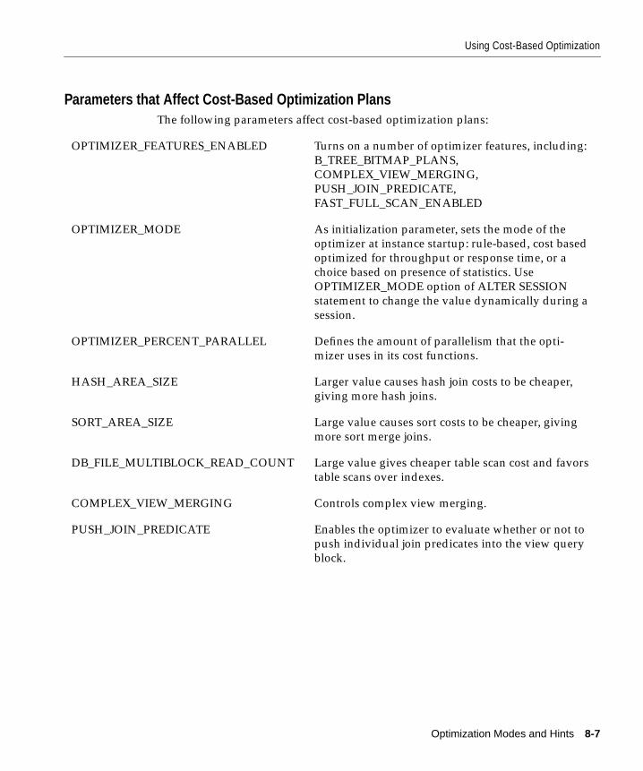
Using Cost-Based Optimization
Parameters that Affect Cost-Based Optimization PlansThe following parameters affect cost-based optimization plans:
OPTIMIZER_FEATURES_ENABLED Turns on a number of optimizer features, including:B_TREE_BITMAP_PLANS,COMPLEX_VIEW_MERGING,PUSH_JOIN_PREDICATE,FAST_FULL_SCAN_ENABLED
OPTIMIZER_MODE As initialization parameter, sets the mode of theoptimizer at instance startup: rule-based, cost basedoptimized for throughput or response time, or achoice based on presence of statistics. UseOPTIMIZER_MODE option of ALTER SESSIONstatement to change the value dynamically during asession.
OPTIMIZER_PERCENT_PARALLEL Defines the amount of parallelism that the opti-mizer uses in its cost functions.
HASH_AREA_SIZE Larger value causes hash join costs to be cheaper,giving more hash joins.
SORT_AREA_SIZE Large value causes sort costs to be cheaper, givingmore sort merge joins.
DB_FILE_MULTIBLOCK_READ_COUNT Large value gives cheaper table scan cost and favorstable scans over indexes.
COMPLEX_VIEW_MERGING Controls complex view merging.
PUSH_JOIN_PREDICATE Enables the optimizer to evaluate whether or not topush individual join predicates into the view queryblock.
Optimization Modes and Hints 8-7
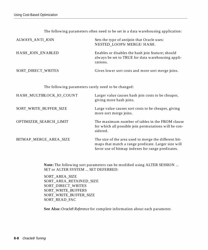
Using Cost-Based Optimization
The following parameters often need to be set in a data warehousing application:
The following parameters rarely need to be changed:
Note: The following sort parameters can be modified using ALTER SESSION ...SET or ALTER SYSTEM ... SET DEFERRED:
SORT_AREA_SIZESORT_AREA_RETAINED_SIZESORT_DIRECT_WRITESSORT_WRITE_BUFFERSSORT_WRITE_BUFFER_SIZESORT_READ_FAC
See Also: Oracle8 Reference for complete information about each parameter.
ALWAYS_ANTI_JOIN Sets the type of antijoin that Oracle uses:NESTED_LOOPS/MERGE/HASH.
HASH_JOIN_ENABLED Enables or disables the hash join feature; shouldalways be set to TRUE for data warehousing appli-cations.
SORT_DIRECT_WRITES Gives lower sort costs and more sort merge joins.
HASH_MULTIBLOCK_IO_COUNT Larger value causes hash join costs to be cheaper,giving more hash joins.
SORT_WRITE_BUFFER_SIZE Large value causes sort costs to be cheaper, givingmore sort merge joins.
OPTIMIZER_SEARCH_LIMIT The maximum number of tables in the FROM clausefor which all possible join permutations will be con-sidered.
BITMAP_MERGE_AREA_SIZE The size of the area used to merge the different bit-maps that match a range predicate. Larger size willfavor use of bitmap indexes for range predicates.
8-8 Oracle8 Tuning
Using Cost-Based Optimization
COMPLEX_VIEW_MERGINGRecommended value: default
When set to FALSE, this parameter causes complex views or subqueries to be evalu-ated before the referencing query. In this case, you can cause a view to be mergedon a per-query basis by using the MERGE hint.
When set to TRUE, this parameter causes complex views or subqueries to bemerged. In this case, you can use the NO_MERGE hint within the view to preventone particular view from being merged. Alternatively, you can use the NO_MERGEhint in the surrounding query, and specify the name of the view that should not bemerged.
PUSH_JOIN_PREDICATERecommended value: TRUE
When this parameter is set to TRUE, the optimizer can evaluate, on a cost basis,whether or not to push individual join predicates into the view query block. Thiscan enable more efficient access path and join methods, such as transforming hashjoins into nested loop joins, and full table scans to index scans.
If PUSH_JOIN_PREDICATE is TRUE, you can use the NO_PUSH_JOIN_PRED hintto prevent pushing join predicates into the view.
If PUSH_JOIN_PREDICATE is FALSE, you can use the PUSH_JOIN_PRED hint toforce pushing of a join predicate into the view.
Tips for Using the Cost-Based ApproachThe cost-based optimization approach assumes that a query will be executed on amultiuser system with a fairly low buffer cache hit rate. Thus a plan selected bycost-based optimization may not be the best plan for a single user system with alarge buffer cache. Timing a query plan on a single user system with a large cachemay not be a good predictor of performance for the same query on a busy mul-tiuser system.
Analyzing a table uses more system resources than analyzing an index. It may behelpful to analyze the indexes for a table separately, with a higher sampling rate.
Use of access path and join method hints invokes cost-based optimization. Sincecost-based optimization is dependent on statistics, it is important to analyze alltables referenced in a query that has hints, even though rule-based optimizationmay have been selected as the system default.
Optimization Modes and Hints 8-9
Using Rule-Based Optimization
Using Rule-Based OptimizationRule-based optimization is supported in Oracle8, but you are advised to write anynew applications using cost-based optimization. Cost-based optimization shouldbe used for new applications and for data warehousing applications, because it sup-ports new and enhanced features. Much of the functionality in Oracle8 (such ashash joins, improved star query processing, and histograms) is available onlythrough cost-based optimization.
If you have developed existing OLTP applications using version 6 of Oracle andhave tuned your SQL statements carefully based on the rules of the optimizer, youmay want to continue using rule-based optimization when you upgrade theseapplications to Oracle8.
If you neither collect statistics nor add hints to your SQL statements, your state-ments will use rule-based optimization. However, you should eventually migrateyour existing applications to use the cost-based approach, because the rule-basedapproach will not be available in future versions of Oracle.
If you are using an application provided by a third-party vendor, check with thevendor to determine which type of optimization is best suited to that application.
You can enable cost-based optimization on a trial basis simply by collecting statis-tics. You can then return to rule-based optimization by deleting them or by settingeither the value of the OPTIMIZER_MODE initialization parameter or theOPTIMIZER_MODE option of the ALTER SESSION command to RULE. You canalso use this value if you want to collect and examine statistics for your data with-out using the cost-based approach.
8-10 Oracle8 Tuning
How to Specify Hints
Introduction to HintsAs an application designer, you may know information about your data that theoptimizer cannot. For example, you may know that a certain index is more selec-tive for certain queries than the optimizer can determine. Based on this informa-tion, you may be able to choose a more efficient execution plan than the optimizercan. In such a case, you can use hints to force the optimizer to use your chosen exe-cution plan.
Hints are suggestions that you give the optimizer for optimizing a SQL statement.Hints allow you to make decisions usually made by the optimizer. You can usehints to specify
■ the optimization approach for a SQL statement
■ the goal of the cost-based approach for a SQL statement
■ the access path for a table accessed by the statement
■ the join order for a join statement
■ a join operation in a join statement
Note, however, that the use of hints involves extra code that must also be managed,checked, controlled.
How to Specify HintsHints apply only to the optimization of the statement block in which they appear.A statement block is any one of the following statements or parts of statements:
■ a simple SELECT, UPDATE, or DELETE statement
■ a parent statement or subquery of a complex statement
■ a part of a compound query
For example, a compound query consisting of two component queries combined bythe UNION operator has two statement blocks, one for each component query. Forthis reason, hints in this first component query apply only to its optimization, notto the optimization of the second component query.
You can send hints for a SQL statement to the optimizer by enclosing them in acomment within the statement.
See Also: For more information on comments, see Oracle8 SQL Reference.
Optimization Modes and Hints 8-11
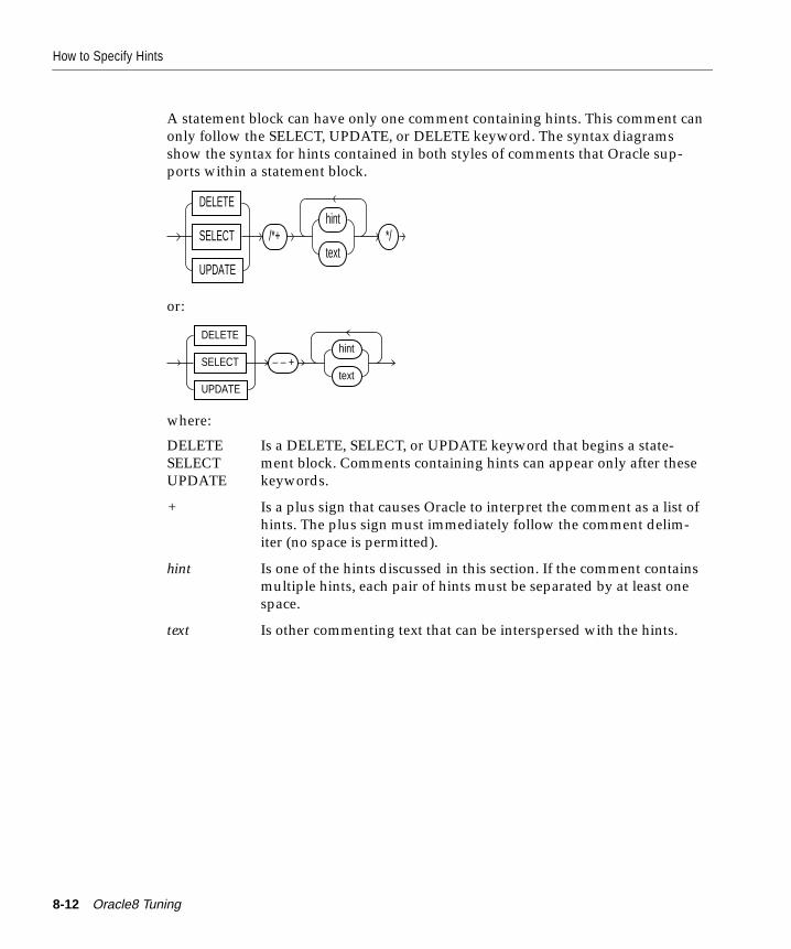
How to Specify Hints
A statement block can have only one comment containing hints. This comment canonly follow the SELECT, UPDATE, or DELETE keyword. The syntax diagramsshow the syntax for hints contained in both styles of comments that Oracle sup-ports within a statement block.
or:
where:
DELETESELECTUPDATE
Is a DELETE, SELECT, or UPDATE keyword that begins a state-ment block. Comments containing hints can appear only after thesekeywords.
+ Is a plus sign that causes Oracle to interpret the comment as a list ofhints. The plus sign must immediately follow the comment delim-iter (no space is permitted).
hint Is one of the hints discussed in this section. If the comment containsmultiple hints, each pair of hints must be separated by at least onespace.
text Is other commenting text that can be interspersed with the hints.
DELETE
SELECT
UPDATE
/*+hint
text*/
DELETE
SELECT
UPDATE
– – +hint
text
8-12 Oracle8 Tuning
How to Specify Hints
If you specify hints incorrectly, Oracle ignores them but does not return an error:
■ Oracle ignores hints if the comment containing them does not follow aDELETE, SELECT, or UPDATE keyword.
■ Oracle ignores hints containing syntax errors, but considers other correctlyspecified hints within the same comment.
■ Oracle ignores combinations of conflicting hints, but considers other hintswithin the same comment.
■ Oracle also ignores hints in all SQL statements in those environments that usePL/SQL Version 1, such as SQL*Forms Version 3 triggers, Oracle Forms 4.5,and Oracle Reports 2.5.
The optimizer recognizes hints only when using the cost-based approach. If youinclude any hint (except the RULE hint) in a statement block, the optimizer auto-matically uses the cost-based approach.
The following sections show the syntax of each hint.
Optimization Modes and Hints 8-13
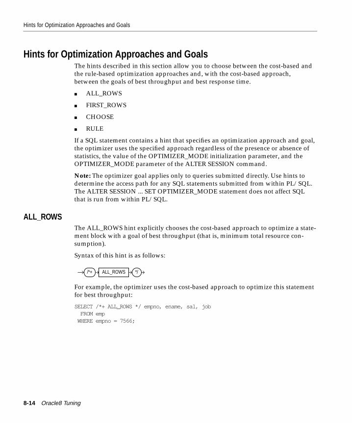
Hints for Optimization Approaches and Goals
Hints for Optimization Approaches and GoalsThe hints described in this section allow you to choose between the cost-based andthe rule-based optimization approaches and, with the cost-based approach,between the goals of best throughput and best response time.
■ ALL_ROWS
■ FIRST_ROWS
■ CHOOSE
■ RULE
If a SQL statement contains a hint that specifies an optimization approach and goal,the optimizer uses the specified approach regardless of the presence or absence ofstatistics, the value of the OPTIMIZER_MODE initialization parameter, and theOPTIMIZER_MODE parameter of the ALTER SESSION command.
Note: The optimizer goal applies only to queries submitted directly. Use hints todetermine the access path for any SQL statements submitted from within PL/SQL.The ALTER SESSION ... SET OPTIMIZER_MODE statement does not affect SQLthat is run from within PL/SQL.
ALL_ROWSThe ALL_ROWS hint explicitly chooses the cost-based approach to optimize a state-ment block with a goal of best throughput (that is, minimum total resource con-sumption).
Syntax of this hint is as follows:
For example, the optimizer uses the cost-based approach to optimize this statementfor best throughput:
SELECT /*+ ALL_ROWS */ empno, ename, sal, job FROM emp WHERE empno = 7566;
/*+ ALL_ROWS */
8-14 Oracle8 Tuning
Hints for Optimization Approaches and Goals
FIRST_ROWSThe FIRST_ROWS hint explicitly chooses the cost-based approach to optimize astatement block with a goal of best response time (minimum resource usage toreturn first row).
This hint causes the optimizer to make these choices:
■ If an index scan is available, the optimizer may choose it over a full table scan.
■ If an index scan is available, the optimizer may choose a nested loops join overa sort-merge join whenever the associated table is the potential inner table ofthe nested loops.
■ If an index scan is made available by an ORDER BY clause, the optimizer maychoose it to avoid a sort operation.
Syntax of this hint is as follows:
For example, the optimizer uses the cost-based approach to optimize this statementfor best response time:
SELECT /*+ FIRST_ROWS */ empno, ename, sal, job FROM emp WHERE empno = 7566;
The optimizer ignores this hint in DELETE and UPDATE statement blocks and inSELECT statement blocks that contain any of the following syntax:
■ set operators (UNION, INTERSECT, MINUS, UNION ALL)
■ GROUP BY clause
■ FOR UPDATE clause
■ group functions
■ DISTINCT operator
These statements cannot be optimized for best response time because Oracle mustretrieve all rows accessed by the statement before returning the first row. If youspecify this hint in any of these statements, the optimizer uses the cost-basedapproach and optimizes for best throughput.
If you specify either the ALL_ROWS or FIRST_ROWS hint in a SQL statement andthe data dictionary contains no statistics about any of the tables accessed by thestatement, the optimizer uses default statistical values (such as allocated storage for
/*+ FIRST_ROWS */
Optimization Modes and Hints 8-15
Hints for Optimization Approaches and Goals
such tables) to estimate the missing statistics and subsequently to choose an execu-tion plan. These estimates may not be as accurate as those generated by the ANA-LYZE command; therefore, you should use the ANALYZE command to generatestatistics for all tables accessed by statements that use cost-based optimization. Ifyou specify hints for access paths or join operations along with either theALL_ROWS or FIRST_ROWS hint, the optimizer gives precedence to the accesspaths and join operations specified by the hints.
CHOOSEThe CHOOSE hint causes the optimizer to choose between the rule-based approachand the cost-based approach for a SQL statement based on the presence of statisticsfor the tables accessed by the statement. If the data dictionary contains statistics forat least one of these tables, the optimizer uses the cost-based approach and opti-mizes with the goal of best throughput. If the data dictionary contains no statisticsfor any of these tables, the optimizer uses the rule-based approach.
Syntax of this hint is as follows:
For example:
SELECT /*+ CHOOSE */ empno, ename, sal, job FROM emp WHERE empno = 7566;
RULEThe RULE hint explicitly chooses rule-based optimization for a statement block. Italso makes the optimizer ignore any other hints specified for the statement block.
Syntax of this hint is as follows:
For example, the optimizer uses the rule-based approach for this statement:
SELECT --+ RULE empno, ename, sal, job FROM emp WHERE empno = 7566;The RULE hint, along with the rule-based approach, may not be supported infuture versions of Oracle.
/*+ CHOOSE */
/*+ RULE */
8-16 Oracle8 Tuning
Hints for Access Methods
Hints for Access MethodsEach hint described in this section suggests an access method for a table.
■ FULL
■ ROWID
■ CLUSTER
■ HASH
■ HASH_AJ
■ INDEX
■ INDEX_ASC
■ INDEX_COMBINE
■ INDEX_DESC
■ INDEX_FFS
■ MERGE_AJ
■ AND_EQUAL
■ USE_CONCAT
Specifying one of these hints causes the optimizer to choose the specified accesspath only if the access path is available based on the existence of an index or clusterand the syntactic constructs of the SQL statement. If a hint specifies an unavailableaccess path, the optimizer ignores it.
You must specify the table to be accessed exactly as it appears in the statement. Ifthe statement uses an alias for the table, you must use the alias, rather than thetable name, in the hint. The table name within the hint should not include theschema name, if the schema name is present in the statement.
FULLThe FULL hint explicitly chooses a full table scan for the specified table.
Syntax of this hint is as follows:
where table specifies the name or alias of the table on which the full table scan is tobe performed.
/* FULL ( table ) */
Optimization Modes and Hints 8-17
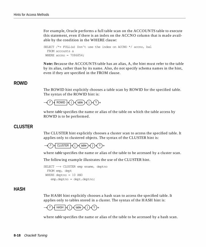
Hints for Access Methods
For example, Oracle performs a full table scan on the ACCOUNTS table to executethis statement, even if there is an index on the ACCNO column that is made avail-able by the condition in the WHERE clause:
SELECT /*+ FULL(a) Don’t use the index on ACCNO */ accno, bal FROM accounts a WHERE accno = 7086854;
Note: Because the ACCOUNTS table has an alias, A, the hint must refer to the tableby its alias, rather than by its name. Also, do not specify schema names in the hint,even if they are specified in the FROM clause.
ROWIDThe ROWID hint explicitly chooses a table scan by ROWID for the specified table.The syntax of the ROWID hint is:
where table specifies the name or alias of the table on which the table access byROWID is to be performed.
CLUSTERThe CLUSTER hint explicitly chooses a cluster scan to access the specified table. Itapplies only to clustered objects. The syntax of the CLUSTER hint is:
where table specifies the name or alias of the table to be accessed by a cluster scan.
The following example illustrates the use of the CLUSTER hint.
SELECT --+ CLUSTER emp ename, deptno FROM emp, dept WHERE deptno = 10 AND emp.deptno = dept.deptno;
HASHThe HASH hint explicitly chooses a hash scan to access the specified table. Itapplies only to tables stored in a cluster. The syntax of the HASH hint is:
where table specifies the name or alias of the table to be accessed by a hash scan.
/* ROWID ( table ) */
/* CLUSTER ( table ) */
/* HASH ( table ) */
8-18 Oracle8 Tuning
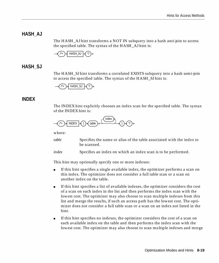
Hints for Access Methods
HASH_AJThe HASH_AJ hint transforms a NOT IN subquery into a hash anti-join to accessthe specified table. The syntax of the HASH_AJ hint is:
HASH_SJThe HASH_SJ hint transforms a correlated EXISTS subquery into a hash semi-jointo access the specified table. The syntax of the HASH_SJ hint is:
INDEXThe INDEX hint explicitly chooses an index scan for the specified table. The syntaxof the INDEX hint is:
where:
This hint may optionally specify one or more indexes:
■ If this hint specifies a single available index, the optimizer performs a scan onthis index. The optimizer does not consider a full table scan or a scan onanother index on the table.
■ If this hint specifies a list of available indexes, the optimizer considers the costof a scan on each index in the list and then performs the index scan with thelowest cost. The optimizer may also choose to scan multiple indexes from thislist and merge the results, if such an access path has the lowest cost. The opti-mizer does not consider a full table scan or a scan on an index not listed in thehint.
■ If this hint specifies no indexes, the optimizer considers the cost of a scan oneach available index on the table and then performs the index scan with thelowest cost. The optimizer may also choose to scan multiple indexes and merge
table Specifies the name or alias of the table associated with the index tobe scanned.
index Specifies an index on which an index scan is to be performed.
/*+ HASH_AJ */
/*+ HASH_SJ */
/*+ INDEX ( tableindex
) */
Optimization Modes and Hints 8-19
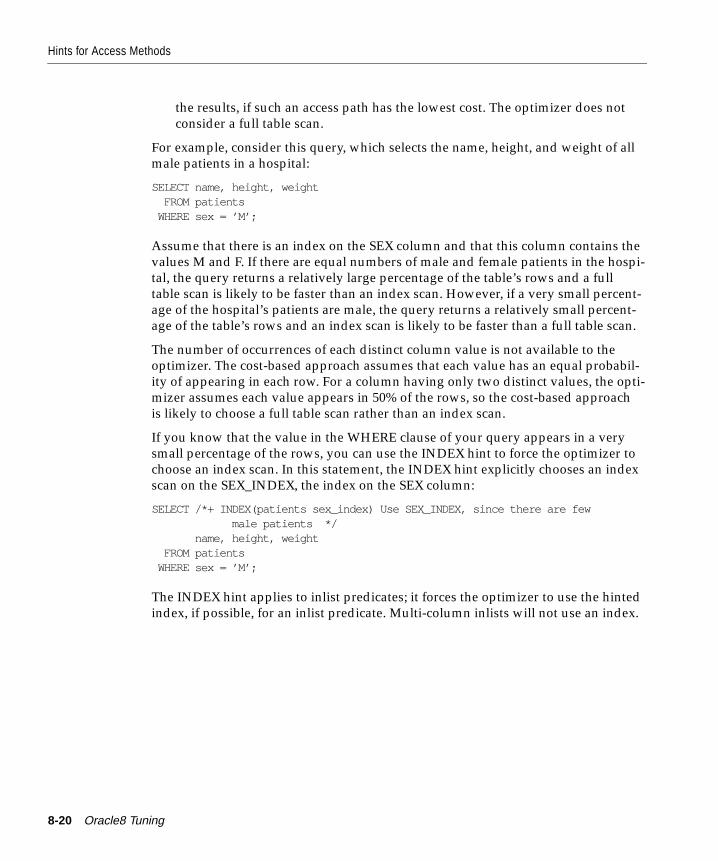
Hints for Access Methods
the results, if such an access path has the lowest cost. The optimizer does notconsider a full table scan.
For example, consider this query, which selects the name, height, and weight of allmale patients in a hospital:
SELECT name, height, weight FROM patients WHERE sex = ’M’;
Assume that there is an index on the SEX column and that this column contains thevalues M and F. If there are equal numbers of male and female patients in the hospi-tal, the query returns a relatively large percentage of the table’s rows and a fulltable scan is likely to be faster than an index scan. However, if a very small percent-age of the hospital’s patients are male, the query returns a relatively small percent-age of the table’s rows and an index scan is likely to be faster than a full table scan.
The number of occurrences of each distinct column value is not available to theoptimizer. The cost-based approach assumes that each value has an equal probabil-ity of appearing in each row. For a column having only two distinct values, the opti-mizer assumes each value appears in 50% of the rows, so the cost-based approachis likely to choose a full table scan rather than an index scan.
If you know that the value in the WHERE clause of your query appears in a verysmall percentage of the rows, you can use the INDEX hint to force the optimizer tochoose an index scan. In this statement, the INDEX hint explicitly chooses an indexscan on the SEX_INDEX, the index on the SEX column:
SELECT /*+ INDEX(patients sex_index) Use SEX_INDEX, since there are few male patients */ name, height, weight FROM patients WHERE sex = ’M’;
The INDEX hint applies to inlist predicates; it forces the optimizer to use the hintedindex, if possible, for an inlist predicate. Multi-column inlists will not use an index.
8-20 Oracle8 Tuning
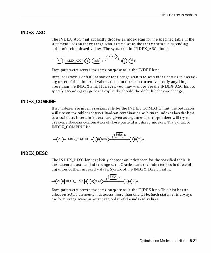
Hints for Access Methods
INDEX_ASCThe INDEX_ASC hint explicitly chooses an index scan for the specified table. If thestatement uses an index range scan, Oracle scans the index entries in ascendingorder of their indexed values. The syntax of the INDEX_ASC hint is:
Each parameter serves the same purpose as in the INDEX hint.
Because Oracle’s default behavior for a range scan is to scan index entries in ascend-ing order of their indexed values, this hint does not currently specify anythingmore than the INDEX hint. However, you may want to use the INDEX_ASC hint tospecify ascending range scans explicitly, should the default behavior change.
INDEX_COMBINEIf no indexes are given as arguments for the INDEX_COMBINE hint, the optimizerwill use on the table whatever Boolean combination of bitmap indexes has the bestcost estimate. If certain indexes are given as arguments, the optimizer will try touse some Boolean combination of those particular bitmap indexes. The syntax ofINDEX_COMBINE is:
INDEX_DESCThe INDEX_DESC hint explicitly chooses an index scan for the specified table. Ifthe statement uses an index range scan, Oracle scans the index entries in descend-ing order of their indexed values. Syntax of the INDEX_DESC hint is:
Each parameter serves the same purpose as in the INDEX hint. This hint has noeffect on SQL statements that access more than one table. Such statements alwaysperform range scans in ascending order of the indexed values.
/*+ INDEX_ASC ( tableindex
) */
/*+ INDEX_COMBINE ( tableindex
) */
/*+ INDEX_DESC ( tableindex
) */
Optimization Modes and Hints 8-21
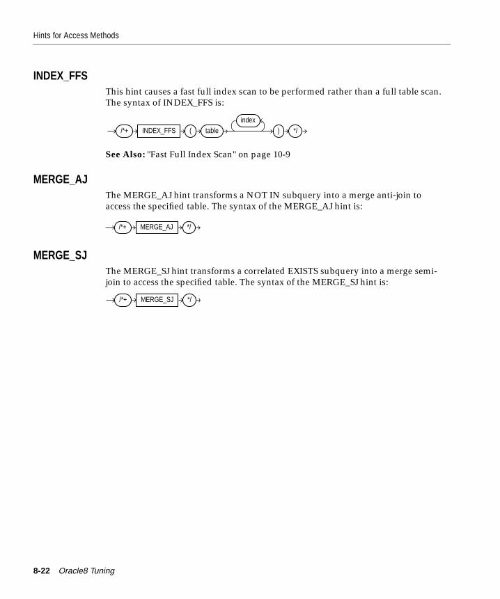
Hints for Access Methods
INDEX_FFSThis hint causes a fast full index scan to be performed rather than a full table scan.The syntax of INDEX_FFS is:
See Also: "Fast Full Index Scan" on page 10-9
MERGE_AJThe MERGE_AJ hint transforms a NOT IN subquery into a merge anti-join toaccess the specified table. The syntax of the MERGE_AJ hint is:
MERGE_SJThe MERGE_SJ hint transforms a correlated EXISTS subquery into a merge semi-join to access the specified table. The syntax of the MERGE_SJ hint is:
/*+ INDEX_FFS ( tableindex
) */
/*+ MERGE_AJ */
/*+ MERGE_SJ */
8-22 Oracle8 Tuning
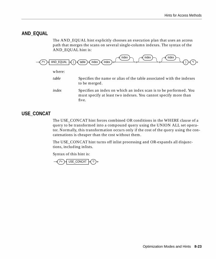
Hints for Access Methods
AND_EQUALThe AND_EQUAL hint explicitly chooses an execution plan that uses an accesspath that merges the scans on several single-column indexes. The syntax of theAND_EQUAL hint is:
where:
USE_CONCATThe USE_CONCAT hint forces combined OR conditions in the WHERE clause of aquery to be transformed into a compound query using the UNION ALL set opera-tor. Normally, this transformation occurs only if the cost of the query using the con-catenations is cheaper than the cost without them.
The USE_CONCAT hint turns off inlist processing and OR-expands all disjunc-tions, including inlists.
Syntax of this hint is:
table Specifies the name or alias of the table associated with the indexesto be merged.
index Specifies an index on which an index scan is to be performed. Youmust specify at least two indexes. You cannot specify more thanfive.
/*+ AND_EQUAL ( table index indexindex index index
) */
/*+ USE_CONCAT */
Optimization Modes and Hints 8-23
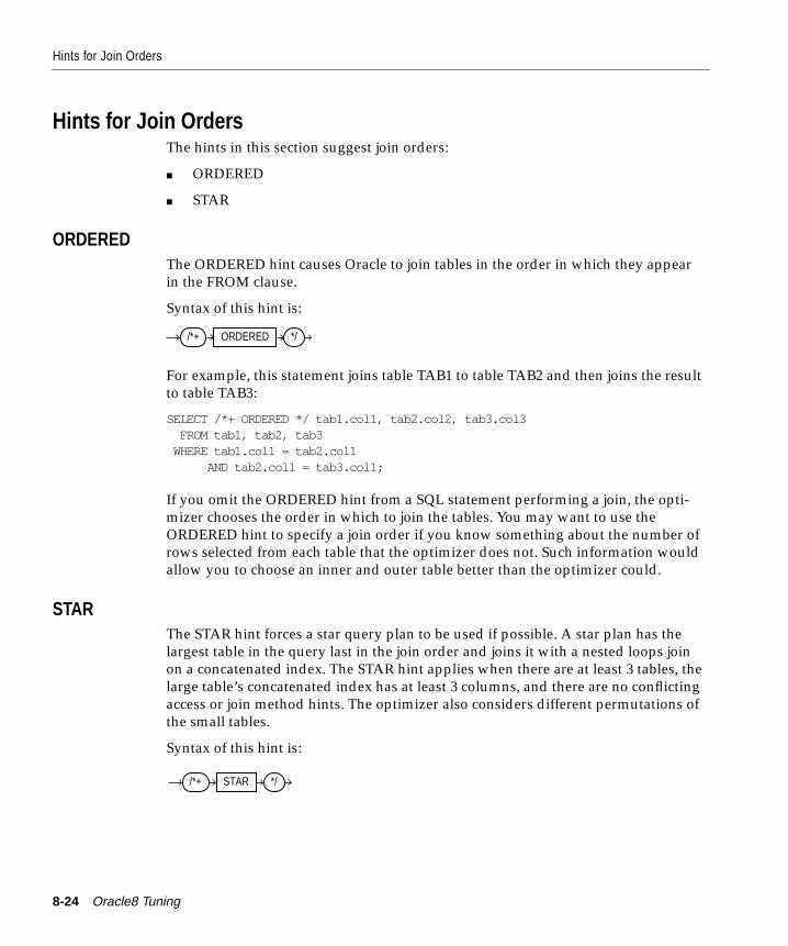
Hints for Join Orders
Hints for Join OrdersThe hints in this section suggest join orders:
■ ORDERED
■ STAR
ORDEREDThe ORDERED hint causes Oracle to join tables in the order in which they appearin the FROM clause.
Syntax of this hint is:
For example, this statement joins table TAB1 to table TAB2 and then joins the resultto table TAB3:
SELECT /*+ ORDERED */ tab1.col1, tab2.col2, tab3.col3 FROM tab1, tab2, tab3 WHERE tab1.col1 = tab2.col1 AND tab2.col1 = tab3.col1;
If you omit the ORDERED hint from a SQL statement performing a join, the opti-mizer chooses the order in which to join the tables. You may want to use theORDERED hint to specify a join order if you know something about the number ofrows selected from each table that the optimizer does not. Such information wouldallow you to choose an inner and outer table better than the optimizer could.
STARThe STAR hint forces a star query plan to be used if possible. A star plan has thelargest table in the query last in the join order and joins it with a nested loops joinon a concatenated index. The STAR hint applies when there are at least 3 tables, thelarge table’s concatenated index has at least 3 columns, and there are no conflictingaccess or join method hints. The optimizer also considers different permutations ofthe small tables.
Syntax of this hint is:
/*+ ORDERED */
/*+ STAR */
8-24 Oracle8 Tuning
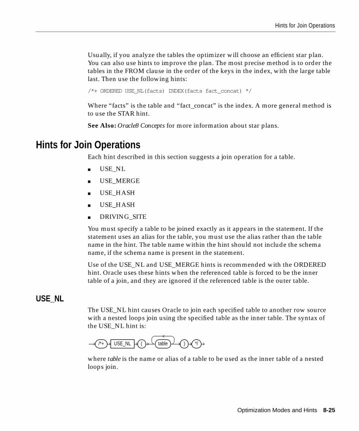
Hints for Join Operations
Usually, if you analyze the tables the optimizer will choose an efficient star plan.You can also use hints to improve the plan. The most precise method is to order thetables in the FROM clause in the order of the keys in the index, with the large tablelast. Then use the following hints:
/*+ ORDERED USE_NL(facts) INDEX(facts fact_concat) */
Where “facts” is the table and “fact_concat” is the index. A more general method isto use the STAR hint.
See Also: Oracle8 Concepts for more information about star plans.
Hints for Join OperationsEach hint described in this section suggests a join operation for a table.
■ USE_NL
■ USE_MERGE
■ USE_HASH
■ USE_HASH
■ DRIVING_SITE
You must specify a table to be joined exactly as it appears in the statement. If thestatement uses an alias for the table, you must use the alias rather than the tablename in the hint. The table name within the hint should not include the schemaname, if the schema name is present in the statement.
Use of the USE_NL and USE_MERGE hints is recommended with the ORDEREDhint. Oracle uses these hints when the referenced table is forced to be the innertable of a join, and they are ignored if the referenced table is the outer table.
USE_NLThe USE_NL hint causes Oracle to join each specified table to another row sourcewith a nested loops join using the specified table as the inner table. The syntax ofthe USE_NL hint is:
where table is the name or alias of a table to be used as the inner table of a nestedloops join.
/*+ USE_NL ( table ) */
Optimization Modes and Hints 8-25
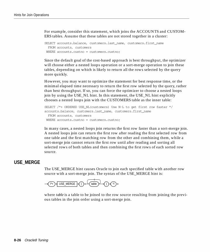
Hints for Join Operations
For example, consider this statement, which joins the ACCOUNTS and CUSTOM-ERS tables. Assume that these tables are not stored together in a cluster:
SELECT accounts.balance, customers.last_name, customers.first_name FROM accounts, customers WHERE accounts.custno = customers.custno;
Since the default goal of the cost-based approach is best throughput, the optimizerwill choose either a nested loops operation or a sort-merge operation to join thesetables, depending on which is likely to return all the rows selected by the querymore quickly.
However, you may want to optimize the statement for best response time, or theminimal elapsed time necessary to return the first row selected by the query, ratherthan best throughput. If so, you can force the optimizer to choose a nested loopsjoin by using the USE_NL hint. In this statement, the USE_NL hint explicitlychooses a nested loops join with the CUSTOMERS table as the inner table:
SELECT /*+ ORDERED USE_NL(customers) Use N-L to get first row faster */accounts.balance, customers.last_name, customers.first_name FROM accounts, customers WHERE accounts.custno = customers.custno;
In many cases, a nested loops join returns the first row faster than a sort-merge join.A nested loops join can return the first row after reading the first selected row fromone table and the first matching row from the other and combining them, while asort-merge join cannot return the first row until after reading and sorting allselected rows of both tables and then combining the first rows of each sorted rowsource.
USE_MERGEThe USE_MERGE hint causes Oracle to join each specified table with another rowsource with a sort-merge join. The syntax of the USE_MERGE hint is:
where table is a table to be joined to the row source resulting from joining the previ-ous tables in the join order using a sort-merge join.
/*+ USE_MERGE ( table ) */
8-26 Oracle8 Tuning
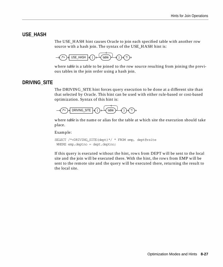
Hints for Join Operations
USE_HASHThe USE_HASH hint causes Oracle to join each specified table with another rowsource with a hash join. The syntax of the USE_HASH hint is:
where table is a table to be joined to the row source resulting from joining the previ-ous tables in the join order using a hash join.
DRIVING_SITEThe DRIVING_SITE hint forces query execution to be done at a different site thanthat selected by Oracle. This hint can be used with either rule-based or cost-basedoptimization. Syntax of this hint is:
where table is the name or alias for the table at which site the execution should takeplace.
Example:
SELECT /*+DRIVING_SITE(dept)*/ * FROM emp, dept@rsite WHERE emp.deptno = dept.deptno;
If this query is executed without the hint, rows from DEPT will be sent to the localsite and the join will be executed there. With the hint, the rows from EMP will besent to the remote site and the query will be executed there, returning the result tothe local site.
/*+ USE_HASH ( table ) */
/*+ DRIVING_SITE ( table ) */
Optimization Modes and Hints 8-27
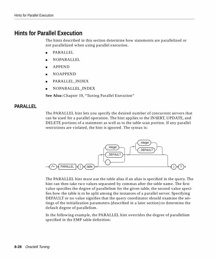
Hints for Parallel Execution
Hints for Parallel ExecutionThe hints described in this section determine how statements are parallelized ornot parallelized when using parallel execution.
■ PARALLEL
■ NOPARALLEL
■ APPEND
■ NOAPPEND
■ PARALLEL_INDEX
■ NOPARALLEL_INDEX
See Also: Chapter 19, “Tuning Parallel Execution”
PARALLELThe PARALLEL hint lets you specify the desired number of concurrent servers thatcan be used for a parallel operation. The hint applies to the INSERT, UPDATE, andDELETE portions of a statement as well as to the table scan portion. If any parallelrestrictions are violated, the hint is ignored. The syntax is:
The PARALLEL hint must use the table alias if an alias is specified in the query. Thehint can then take two values separated by commas after the table name. The firstvalue specifies the degree of parallelism for the given table, the second value speci-fies how the table is to be split among the instances of a parallel server. SpecifyingDEFAULT or no value signifies that the query coordinator should examine the set-tings of the initialization parameters (described in a later section) to determine thedefault degree of parallelism.
In the following example, the PARALLEL hint overrides the degree of parallelismspecified in the EMP table definition:
/*+ PARALLEL ( table
, integer
, DEFAULT
,
, integer
, DEFAULT
) */
8-28 Oracle8 Tuning
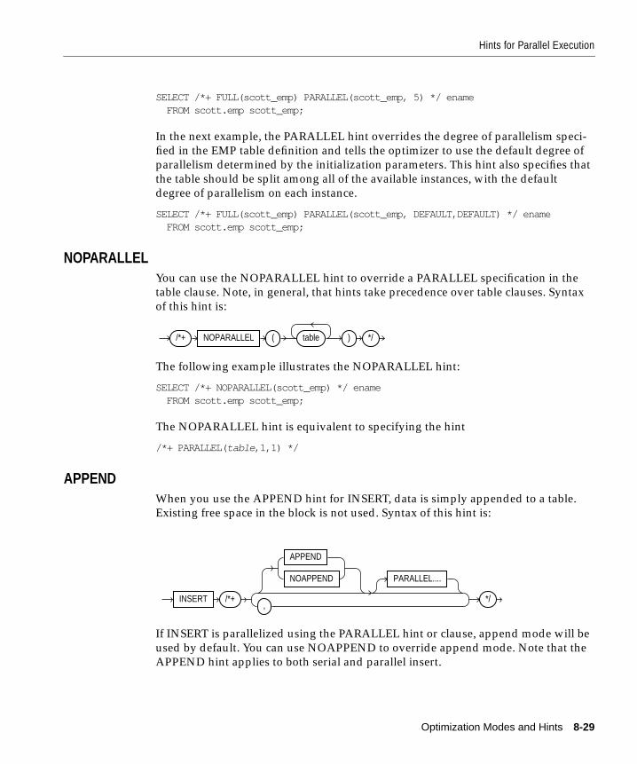
Hints for Parallel Execution
SELECT /*+ FULL(scott_emp) PARALLEL(scott_emp, 5) */ ename FROM scott.emp scott_emp;
In the next example, the PARALLEL hint overrides the degree of parallelism speci-fied in the EMP table definition and tells the optimizer to use the default degree ofparallelism determined by the initialization parameters. This hint also specifies thatthe table should be split among all of the available instances, with the defaultdegree of parallelism on each instance.
SELECT /*+ FULL(scott_emp) PARALLEL(scott_emp, DEFAULT,DEFAULT) */ ename FROM scott.emp scott_emp;
NOPARALLELYou can use the NOPARALLEL hint to override a PARALLEL specification in thetable clause. Note, in general, that hints take precedence over table clauses. Syntaxof this hint is:
The following example illustrates the NOPARALLEL hint:
SELECT /*+ NOPARALLEL(scott_emp) */ ename FROM scott.emp scott_emp;
The NOPARALLEL hint is equivalent to specifying the hint
/*+ PARALLEL( table ,1,1) */
APPENDWhen you use the APPEND hint for INSERT, data is simply appended to a table.Existing free space in the block is not used. Syntax of this hint is:
If INSERT is parallelized using the PARALLEL hint or clause, append mode will beused by default. You can use NOAPPEND to override append mode. Note that theAPPEND hint applies to both serial and parallel insert.
/*+ NOPARALLEL ( table ) */
INSERT /*+
APPEND
NOAPPEND PARALLEL....
,*/
Optimization Modes and Hints 8-29
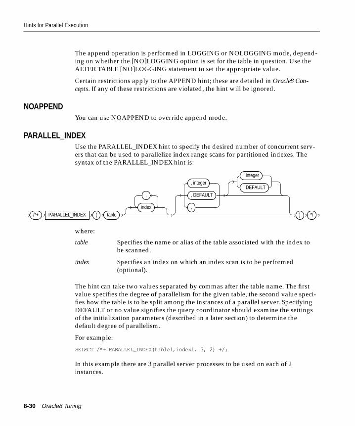
Hints for Parallel Execution
The append operation is performed in LOGGING or NOLOGGING mode, depend-ing on whether the [NO]LOGGING option is set for the table in question. Use theALTER TABLE [NO]LOGGING statement to set the appropriate value.
Certain restrictions apply to the APPEND hint; these are detailed in Oracle8 Con-cepts. If any of these restrictions are violated, the hint will be ignored.
NOAPPENDYou can use NOAPPEND to override append mode.
PARALLEL_INDEXUse the PARALLEL_INDEX hint to specify the desired number of concurrent serv-ers that can be used to parallelize index range scans for partitioned indexes. Thesyntax of the PARALLEL_INDEX hint is:
where:
The hint can take two values separated by commas after the table name. The firstvalue specifies the degree of parallelism for the given table, the second value speci-fies how the table is to be split among the instances of a parallel server. SpecifyingDEFAULT or no value signifies the query coordinator should examine the settingsof the initialization parameters (described in a later section) to determine thedefault degree of parallelism.
For example:
SELECT /*+ PARALLEL_INDEX(table1,index1, 3, 2) +/;
In this example there are 3 parallel server processes to be used on each of 2instances.
table Specifies the name or alias of the table associated with the index tobe scanned.
index Specifies an index on which an index scan is to be performed(optional).
/*+ PARALLEL_INDEX ( tableindex
,
, integer
, DEFAULT
,
, integer
, DEFAULT
) */
8-30 Oracle8 Tuning
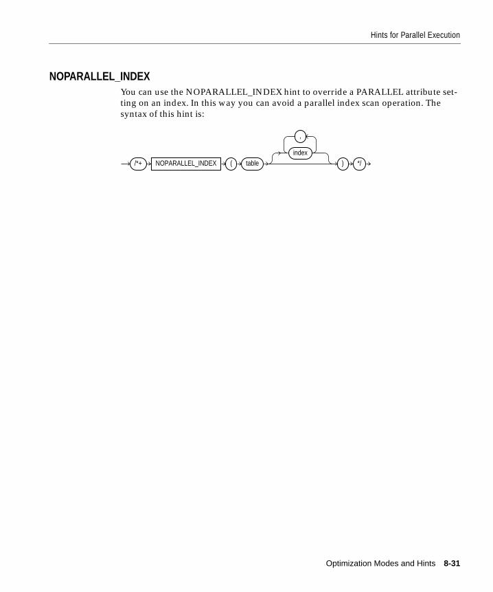
Hints for Parallel Execution
NOPARALLEL_INDEXYou can use the NOPARALLEL_INDEX hint to override a PARALLEL attribute set-ting on an index. In this way you can avoid a parallel index scan operation. Thesyntax of this hint is:
/*+ NOPARALLEL_INDEX ( tableindex
,
) */
Optimization Modes and Hints 8-31
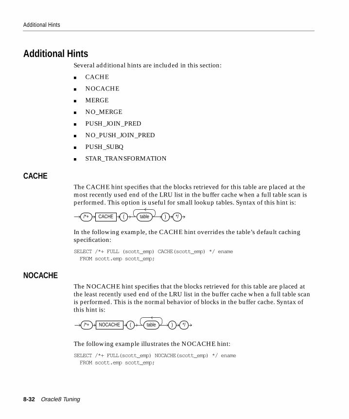
Additional Hints
Additional HintsSeveral additional hints are included in this section:
■ CACHE
■ NOCACHE
■ MERGE
■ NO_MERGE
■ PUSH_JOIN_PRED
■ NO_PUSH_JOIN_PRED
■ PUSH_SUBQ
■ STAR_TRANSFORMATION
CACHEThe CACHE hint specifies that the blocks retrieved for this table are placed at themost recently used end of the LRU list in the buffer cache when a full table scan isperformed. This option is useful for small lookup tables. Syntax of this hint is:
In the following example, the CACHE hint overrides the table’s default cachingspecification:
SELECT /*+ FULL (scott_emp) CACHE(scott_emp) */ ename FROM scott.emp scott_emp;
NOCACHEThe NOCACHE hint specifies that the blocks retrieved for this table are placed atthe least recently used end of the LRU list in the buffer cache when a full table scanis performed. This is the normal behavior of blocks in the buffer cache. Syntax ofthis hint is:
The following example illustrates the NOCACHE hint:
SELECT /*+ FULL(scott_emp) NOCACHE(scott_emp) */ ename FROM scott.emp scott_emp;
/*+ CACHE ( table ) */
/*+ NOCACHE ( table ) */
8-32 Oracle8 Tuning

Additional Hints
MERGEWhen the COMPLEX_VIEW_MERGING parameter is set to FALSE, this parametercauses complex views or subqueries to be evaluated before the surrounding query.In this case, you can cause a view to be merged on a per-query basis by using theMERGE hint. Syntax of this hint is:
For example:
SELECT /*+ MERGE(v) */ t1.x, v.avg_yFROM t1
(SELECT x, avg(y) AS avg_yFROM t2GROUP BY x) v
WHERE t1.x = v.x AND t1.y = 1;
NO_MERGEThe NO_MERGE hint causes Oracle not to merge mergeable views. The syntax ofthe NO_MERGE hint is:
This hint allows the user to have more influence over the way in which the viewwill be accessed. For example,
SELECT /*+ NO_MERGE(v) */ t1.x, v.avg_yFROM t1
(SELECT x, avg(y) AS avg_yFROM t2GROUP BY x) v
WHERE t1.x = v.x AND t1.y = 1;
causes view v not to be merged.
When COMPLEX_VIEW_MERGING is set to TRUE, you can use the NO_MERGEhint within the view to prevent one particular query from being merged.
When the NO_MERGE hint is used without an argument, it should be placed in theview query block. When NO_MERGE is used with the view name as an argument,it should be placed in the surrounding query.
/*+ MERGE ( table ) */
/*+ NO_MERGE ( table ) */
Optimization Modes and Hints 8-33
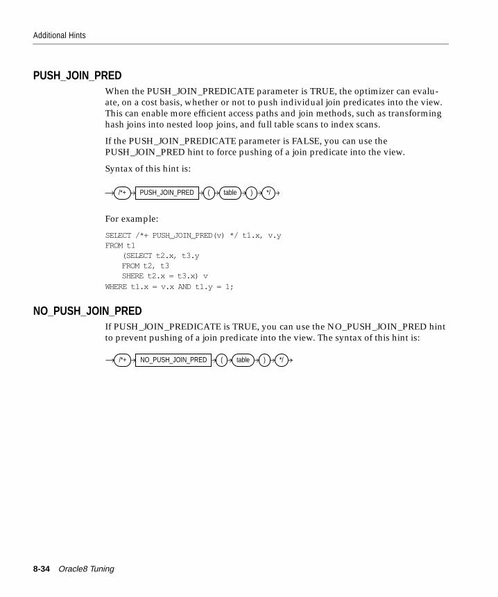
Additional Hints
PUSH_JOIN_PREDWhen the PUSH_JOIN_PREDICATE parameter is TRUE, the optimizer can evalu-ate, on a cost basis, whether or not to push individual join predicates into the view.This can enable more efficient access paths and join methods, such as transforminghash joins into nested loop joins, and full table scans to index scans.
If the PUSH_JOIN_PREDICATE parameter is FALSE, you can use thePUSH_JOIN_PRED hint to force pushing of a join predicate into the view.
Syntax of this hint is:
For example:
SELECT /*+ PUSH_JOIN_PRED(v) */ t1.x, v.yFROM t1
(SELECT t2.x, t3.yFROM t2, t3SHERE t2.x = t3.x) v
WHERE t1.x = v.x AND t1.y = 1;
NO_PUSH_JOIN_PREDIf PUSH_JOIN_PREDICATE is TRUE, you can use the NO_PUSH_JOIN_PRED hintto prevent pushing of a join predicate into the view. The syntax of this hint is:
/*+ PUSH_JOIN_PRED ( table ) */
/*+ NO_PUSH_JOIN_PRED ( table ) */
8-34 Oracle8 Tuning
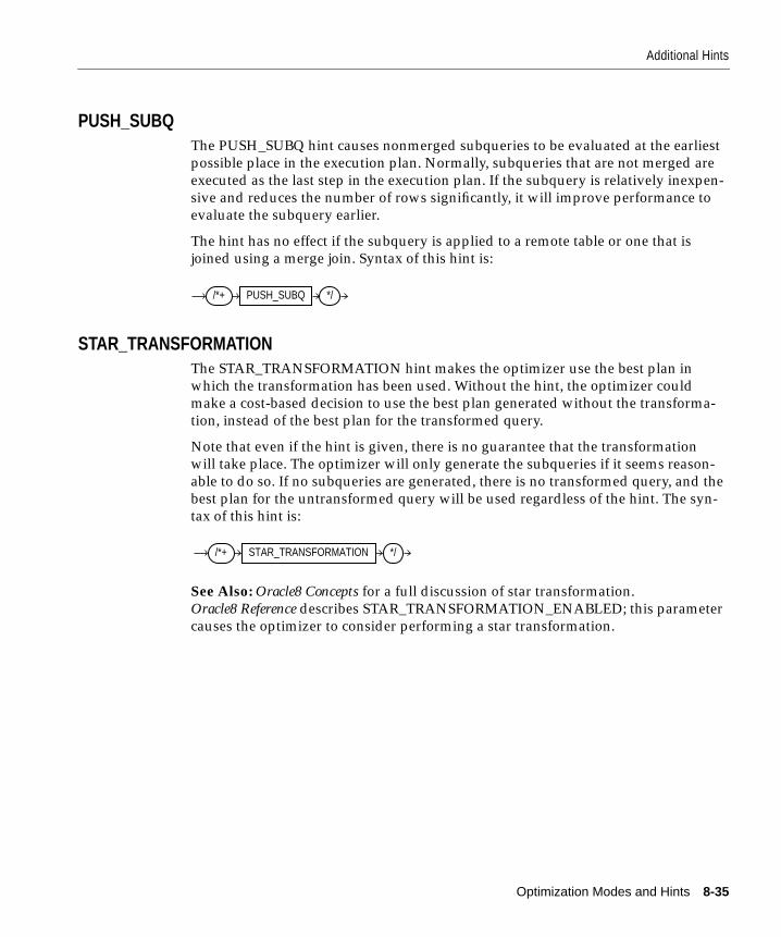
Additional Hints
PUSH_SUBQThe PUSH_SUBQ hint causes nonmerged subqueries to be evaluated at the earliestpossible place in the execution plan. Normally, subqueries that are not merged areexecuted as the last step in the execution plan. If the subquery is relatively inexpen-sive and reduces the number of rows significantly, it will improve performance toevaluate the subquery earlier.
The hint has no effect if the subquery is applied to a remote table or one that isjoined using a merge join. Syntax of this hint is:
STAR_TRANSFORMATIONThe STAR_TRANSFORMATION hint makes the optimizer use the best plan inwhich the transformation has been used. Without the hint, the optimizer couldmake a cost-based decision to use the best plan generated without the transforma-tion, instead of the best plan for the transformed query.
Note that even if the hint is given, there is no guarantee that the transformationwill take place. The optimizer will only generate the subqueries if it seems reason-able to do so. If no subqueries are generated, there is no transformed query, and thebest plan for the untransformed query will be used regardless of the hint. The syn-tax of this hint is:
See Also: Oracle8 Concepts for a full discussion of star transformation.Oracle8 Reference describes STAR_TRANSFORMATION_ENABLED; this parametercauses the optimizer to consider performing a star transformation.
/*+ PUSH_SUBQ */
/*+ STAR_TRANSFORMATION */
Optimization Modes and Hints 8-35
Using Hints with Views
Using Hints with ViewsOracle Corporation does not encourage users to use hints inside or on views (orsubqueries). This is because views can be defined in one context and used inanother; such hints can result in unexpected plans. In particular, hints inside viewsor on views are handled differently depending on whether or not the view is merge-able into the top-level query.
Should you decide, nonetheless, to use hints with views, the following sectionsdescribe the behavior in each case.
■ Hints and Mergeable Views
■ Hints and Nonmergeable Views
Hints and Mergeable ViewsThis section describes hint behavior with mergeable views.
Optimization Approaches and Goal HintsOptimization approach and goal hints can occur in a top-level query or insideviews.
■ If there is such a hint in the top-level query, that hint is used regardless of anysuch hints inside the views.
■ If there is no top-level optimizer mode hint, then mode hints in referencedviews are used as long as all mode hints in the views are consistent.
■ If two or more mode hints in the referenced views conflict, then all mode hintsin the views are discarded and the session mode is used, whether default oruser-specified.
Access Method and Join Hints on ViewsAccess method and join hints on referenced views are ignored unless the view con-tains a single table (or references another view with a single table). For such single-table views, an access method hint or a join hint on the view applies to the tableinside the view.
8-36 Oracle8 Tuning
Using Hints with Views
Access Method and Join Hints Inside ViewsAccess method and join hints can appear in a view definition.
■ If the view is a subquery (that is, if it appears in the FROM clause of a SELECTstatement), then all access method and join hints inside the view are preservedwhen the view is merged with the top-level query.
■ For views that are not subqueries, access method and join hints in the view arepreserved only if the top-level query references no other tables or views (thatis, if the FROM clause of the SELECT statement contains only the view).
Parallel Execution Hints on ViewsPARALLEL, NOPARALLEL, PARALLEL_INDEX and NOPARALLEL_INDEXhints on views are always recursively applied to all the tables in the referencedview. Parallel execution hints in a top-level query override such hints inside a refer-enced view.
Hints and Nonmergeable ViewsWith nonmergeable views, optimization approach and goal hints inside the vieware ignored: the top-level query decides the optimization mode.
Since nonmergeable views are optimized separately from the top-level query,access method and join hints inside the view are always preserved. For the samereason, access method hints on the view in the top-level query are ignored.
However, join hints on the view in the top-level query are preserved since, in thiscase, a nonmergeable view is similar to a table.
Optimization Modes and Hints 8-37

Using Hints with Views
8-38 Oracle8 Tuning
Tuning Distributed Qu
9
Tuning Distributed QueriesOracle supports transparent distributed queries to access data from multiple data-bases. It also provides many other distributed features, such as transparent distrib-uted transactions and a transparent fully automatic two-phase commit. Thischapter explains how the Oracle8 optimizer decomposes SQL statements, and howthis affects performance of distributed queries. The chapter provides guidelines onhow to influence the optimizer and avoid performance bottlenecks.
Topics include:
■ Remote and Distributed Queries
■ Distributed Query Restrictions
■ Transparent Gateways
■ Summary: Optimizing Performance of Distributed Queries
eries 9-1
Remote and Distributed Queries
Remote and Distributed QueriesIf a SQL statement references one or more remote tables, the optimizer first deter-mines whether all remote tables are located at the same site. If all tables are locatedat the same remote site, Oracle sends the entire query to the remote site for execu-tion. The remote site sends the resulting rows back to the local site. This is called aremote SQL statement. If the tables are located at more than one site, the optimizerdecomposes the query into separate SQL statements to access each of the remotetables. This is called a distributed SQL statement. The site where the query is exe-cuted, called the “driving site,” is normally the local site.
This section describes:
■ Remote Data Dictionary Information
■ Remote SQL Statements
■ Distributed SQL Statements
■ EXPLAIN PLAN and SQL Decomposition
■ Partition Views
Remote Data Dictionary InformationIf a SQL statement references multiple tables, then the optimizer must determinewhich columns belong to which tables before it can decompose the SQL statement.For example, with
SELECT DNAME, ENAME FROM DEPT, EMP@REMOTE WHERE DEPT.DEPTNO = EMP.DEPTNO
the optimizer must first determine that the DNAME column belongs to the DEPTtable and the ENAME column to the EMP table. Once the optimizer has the datadictionary information of all remote tables, it can build the decomposed SQL state-ments.
Column and table names in decomposed SQL statements appear between doublequotes. You must enclose in double quotes any column and table names that con-tain special characters, reserved words, or spaces.
This mechanism also replaces an asterisk (*) in the select list with the actual columnnames. For example:
SELECT * FROM DEPT@REMOTE;
9-2 Oracle8 Tuning
Remote and Distributed Queries
results in the decomposed SQL statement
SELECT A1."DEPTNO", A1."DNAME", A1."LOC" FROM "DEPT" A1;
Note: For the sake of simplicity, double quotes are not used in the remainder of thischapter.
Remote SQL StatementsIf the entire SQL statement is sent to the remote database, the optimizer uses tablealiases A1, A2, and so on, for all tables and columns in the query, in order to avoidpossible naming conflicts. For example:
SELECT DNAME, ENAME FROM DEPT@REMOTE, EMP@REMOTE WHERE DEPT.DEPTNO = EMP.DEPTNO;
is sent to the remote database as
SELECT A2.DNAME, A1.ENAME FROM DEPT A2, EMP A1 WHERE A1.DEPTNO = A2.DEPTNO;
Tuning Distributed Queries 9-3
Remote and Distributed Queries
Distributed SQL StatementsWhen a query accesses data on one or more databases, one site “drives” the execu-tion of the query. This is known as the “driving site”; it is here that the data isjoined, grouped and ordered. By default, the local Oracle server will be the drivingsite. A hint called DRIVING_SITE enables you to manually specify the driving site.
The decomposition of SQL statements is important because it determines the num-ber of records or even tables that must be sent through the network. A knowledgeof how the optimizer decomposes SQL statements can help you achieve optimumperformance for distributed queries.
If a SQL statement references one or more remote tables, the optimizer must decom-pose the SQL statement into separate queries to be executed on the different data-bases. For example:
SELECT DNAME, ENAMEFROM DEPT, EMP@REMOTEWHERE DEPT.DEPTNO = EMP.DEPTNO;
might be decomposed into
SELECT DEPTNO, DNAME FROM DEPT;
which is executed locally, and
SELECT DEPTNO, ENAME FROM EMP;
which is sent to the remote database. The data from both tables is joined locally. Allthis is done automatically and transparently for the user or application.
In some cases, however, it might be better to send the local table to the remote data-base and join the two tables on the remote database. This can be achieved either bycreating a view, or by using the DRIVING_SITE hint. If you decide to create a viewon the remote database, a database link from the remote database to the local data-base is also needed.
For example (on the remote database):
CREATE VIEW DEPT_EMP ASSELECT DNAME, ENAMEFROM DEPT@LOCAL, EMPWHERE DEPT.DEPTNO = EMP.DEPTNO;
Then select from the remote view instead of the local and remote tables
SELECT * FROM DEPT_EMP@REMOTE;
9-4 Oracle8 Tuning
Remote and Distributed Queries
Now the local DEPT table is sent through the network to the remote database,joined on the remote database with the EMP table, and the result is sent back to thelocal database.
See Also: "DRIVING_SITE" on page 8-27 for details about this hint.
Rule-Based OptimizationRule-based optimization does not have information about indexes for remotetables. It never, therefore, generates a nested loops join between a local table and aremote table with the local table as the outer table in the join. It uses either a nestedloops join with the remote table as the outer table or a sort merge join, dependingon the indexes available for the local table.
Cost-Based OptimizationCost-based optimization can consider more execution plans than rule-based optimi-zation. Cost-based optimization knows whether indexes on remote tables are avail-able, and in which cases it would make sense to use them. Cost-based optimizationconsiders index access of the remote tables as well as full table scans, whereas rule-based optimization considers only full table scans.
The particular execution plan and table access that cost-based optimization choosesdepends on the table and index statistics. For example, with
SELECT DNAME, ENAME FROM DEPT, EMP@REMOTE WHERE DEPT.DEPTNO = EMP.DEPTNO
the optimizer might choose the local DEPT table as the driving table and access theremote EMP table using an index. In that case the decomposed SQL statementbecomes
SELECT ENAME FROM EMP WHERE DEPTNO = :1
This decomposed SQL statement is used for a nested loops operation.
Tuning Distributed Queries 9-5
Remote and Distributed Queries
Using ViewsIf tables are on more than one remote site, it can be more effective to create a viewthan to use the DRIVING_SITE hint. If not all tables are on the same remote data-base, the optimizer accesses each remote table separately. For example:
SELECT D.DNAME, E1.ENAME, E2.JOB FROM DEPT D, EMP@REMOTE E1, EMP@REMOTE E2 WHERE D.DEPTNO = E1.DEPTNO AND E1.MGR = E2.EMPNO;
results in the decomposed SQL statements
SELECT EMPNO, ENAME FROM EMP;
and
SELECT ENAME, MGR, DEPTNO FROM EMP;
If you want to join the two EMP tables remotely, you can create a view to accom-plish this. Create a view with the join of the remote tables on the remote database.For example (on the remote database):
CREATE VIEW EMPS ASSELECT E1.DEPTNO, E1.ENAME, E2.JOB FROM EMP E1, EMP E2 WHERE E1.MGR = E2.EMPNO;
and now select from the remote view instead of the remote tables:
SELECT D.DNAME, E.ENAME, E.JOB FROM DEPT D, EMPS@REMOTE E WHERE D.DEPTNO = E.DEPTNO;
This results in the decomposed SQL statement
SELECT DEPTNO, ENAME, JOB FROM EMPS;
Using HintsIn a distributed query, all hints are supported for local tables. For remote tables,however, you can use only join order and join operation hints. (Hints for accessmethods, parallel hints, and so on, have no effect.) For remote mapped queries, allhints are supported.
See Also: "Hints for Join Orders" on page 8-24"Hints for Join Operations" on page 8-25
9-6 Oracle8 Tuning
Remote and Distributed Queries
EXPLAIN PLAN and SQL DecompositionEXPLAIN PLAN gives information not only about the overall execution plan ofSQL statements, but also about the way in which the optimizer decomposes SQLstatements. EXPLAIN PLAN stores information in the PLAN_TABLE table. Ifremote tables are used in a SQL statement, the OPERATION column will containthe value REMOTE to indicate that a remote table is referenced, and the OTHERcolumn will contain the decomposed SQL statement that will be sent to the remotedatabase. For example:
EXPLAIN PLAN FOR SELECT DNAME FROM DEPT@REMOTESELECT OPERATION, OTHER FROM PLAN_TABLE
OPERATION OTHER--------- -------------------------------------REMOTE SELECT A1."DNAME" FROM "DEPT" A1
Note the table alias and the double quotes around the column and table names.
See Also: Chapter 23, “The EXPLAIN PLAN Command”
Tuning Distributed Queries 9-7
Remote and Distributed Queries
Partition ViewsYou can utilize partition views to bring together tables that have the same struc-ture, but contain different partitions of data. This can be very useful for a distrib-uted database system, where each partition resides on a database and the data ineach partition has common geographical properties.
When a query is executed on such a partition view, and the query contains a predi-cate that contains the result set to a subset of the view’s partitions, the optimizerchooses a plan which skips partitions that are not needed for the query. This parti-tion elimination takes place at run time, when the execution plan references all par-titions.
Rules for UseThis section describes the circumstances under which a UNION ALL view enablesthe optimizer to skip partitions. The Oracle server that contains the partition viewmust conform to the following rules:
■ The PARTITION_VIEW_ENABLED initialization parameter is set to TRUE
■ The cost-based optimizer is used.
Note: To use the cost-based optimizer you must analyze all tables used in theUNION ALL views. Alternatively, you can use a hint or set the parameterOPTIMIZER_MODE to ALL_ROWS or FIRST_ROW. To set OPTIMIZER_MODE orPARTITION_VIEW_ENABLED you can also use the ALTER SESSION statement.
Within a UNION ALL view there are multiple select statements, and each of theseis called a “branch”. A UNION ALL view is a partition view if each select state-ment it defines conforms to the following rules:
■ The branch has exactly one table in the FROM clause.
■ The branch contains a WHERE clause that defines the subset of data from thepartition that is contained in the view.
■ None of the following are used within the branch: WHERE clause with sub-query, group by, aggregate functions, distinct, rownum, connect by/start with.
■ The SELECT list of each branch is *, or explicit expansion of "*".
■ The column names and column datatypes for all branches in the UNION ALLview are exactly the same.
■ All tables used in the branch must have indexes (if any) on the same columnsand number of columns.
9-8 Oracle8 Tuning
Remote and Distributed Queries
Partition elimination is based on column transitivity with constant predicates. TheWHERE clause used in the query that accesses the partition view is pushed downto the WHERE clause of each of the branches in the UNION ALL view definition.Consider the following example:
SELECT * FROM EMP_VIEW WHERE deptno=30;
when the view EMP_VIEW is defined as
SELECT * FROM EMP@d10 WHERE deptno=10UNION ALLSELECT * FROM EMP@d20 WHERE deptno=20UNION ALLSELECT * FROM EMP@d30 WHERE deptno=30UNION ALLSELECT * FROM EMP@d40 WHERE deptno=40
The "WHERE deptno=30" predicate used in the query is pushed down to the que-ries in the UNION ALL view. For a WHERE clause such as "WHERE deptno=10and deptno=30", the optimizer applies transitivity rules to generate an extra predi-cate of "10=30". This extra predicate is always false, thus the table (EMP@d10) neednot be accessed.
Transitivity applies to predicates which conform to the following rules:
■ The predicates in the WHERE clause for each branch are of the form
relation AND relation ...
where relation is of the form
column_name relop constant_expression
and relop is one of =, !=, >, >=, <, <=
Note that BETWEEN ... AND is allowed by these rules, but IN is not.
■ At least one predicate in the query referencing the view exists in the same form.
Tuning Distributed Queries 9-9
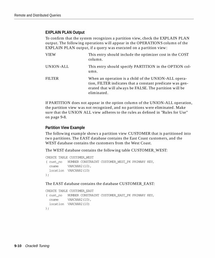
Remote and Distributed Queries
EXPLAIN PLAN OutputTo confirm that the system recognizes a partition view, check the EXPLAIN PLANoutput. The following operations will appear in the OPERATIONS column of theEXPLAIN PLAN output, if a query was executed on a partition view:
If PARTITION does not appear in the option column of the UNION-ALL operation,the partition view was not recognized, and no partitions were eliminated. Makesure that the UNION ALL view adheres to the rules as defined in "Rules for Use"on page 9-8.
Partition View ExampleThe following example shows a partition view CUSTOMER that is partitioned intotwo partitions. The EAST database contains the East Coast customers, and theWEST database contains the customers from the West Coast.
The WEST database contains the following table CUSTOMER_WEST:
CREATE TABLE CUSTOMER_WEST( cust_no NUMBER CONSTRAINT CUSTOMER_WEST_PK PRIMARY KEY, cname VARCHAR2(10), location VARCHAR2(10));
The EAST database contains the database CUSTOMER_EAST:
CREATE TABLE CUSTOMER_EAST( cust_no NUMBER CONSTRAINT CUSTOMER_EAST_PK PRIMARY KEY, cname VARCHAR2(10), location VARCHAR2(10));
VIEW This entry should include the optimizer cost in the COSTcolumn.
UNION-ALL This entry should specify PARTITION in the OPTION col-umn.
FILTER When an operation is a child of the UNION-ALL opera-tion, FILTER indicates that a constant predicate was gen-erated that will always be FALSE. The partition will beeliminated.
9-10 Oracle8 Tuning
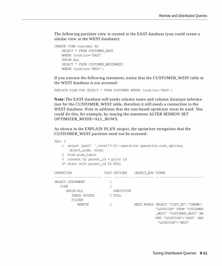
Remote and Distributed Queries
The following partition view is created at the EAST database (you could create asimilar view at the WEST database):
CREATE VIEW customer ASSELECT * FROM CUSTOMER_EASTWHERE location='EAST'UNION ALLSELECT * FROM CUSTOMER_WEST@WESTWHERE location='WEST';
If you execute the following statement, notice that the CUSTOMER_WEST table inthe WEST database is not accessed:
EXPLAIN PLAN FOR SELECT * FROM CUSTOMER WHERE location='EAST';
Note: The EAST database still needs column name and column datatype informa-tion for the CUSTOMER_WEST table, therefore it still needs a connection to theWEST database. Note in addition that the cost-based optimizer must be used. Youcould do this, for example, by issuing the statement ALTER SESSION SETOPTIMIZER_MODE=ALL_ROWS.
As shown in the EXPLAIN PLAN output, the optimizer recognizes that theCUSTOMER_WEST partition need not be accessed:
SQL> r1 select lpad(' ',level*3-3)||operation operation,cost,options,
object_node, other2 from plan_table3 connect by parent_id = prior id4* start with parent_id IS NULL
OPERATION COST OPTIONS OBJECT_NOD OTHER------------------------- ---- ---------- ---------- -------------------------SELECT STATEMENT 1 VIEW 1 UNION-ALL PARTITION TABLE ACCESS 1 FULL FILTER REMOTE 1 WEST.WORLD SELECT "CUST_NO","CNAME", "LOCATION" FROM "CUSTOMER _WEST" "CUSTOMER_WEST" WH ERE "LOCATION"='EAST' AND "LOCATION"='WEST'
Tuning Distributed Queries 9-11
Distributed Query Restrictions
Distributed Query RestrictionsDistributed queries within the same version of Oracle have these restrictions:
■ Cost-based optimization should be used for distributed queries. Rule-basedoptimization does not generate nested loop joins between remote and localtables when the tables are joined with equijoins.
■ In cost-based optimization, no more than 20 indexes per remote table are con-sidered when generating query plans. The order of the indexes varies; if the 20-index limitation is exceeded, random variation in query plans may result.
■ Reverse indexes on remote tables are not visible to the optimizer. This can pre-vent nested-loop joins from being used for remote tables if there is an equijoinusing a column with only a reverse index.
■ Cost-based optimization cannot recognize that a remote object is partitioned.Thus the optimizer may generate less than optimal plans for remote parti-tioned objects, particularly when partition pruning would have been possible,had the object been local.
■ Remote views are not merged and the optimizer has no statistics for them. It isbest to replicate all mergeable views at all sites to obtain good query plans. (Seethe following exception.)
■ Neither cost-based nor rule-based optimization can execute joins remotely. Alljoins are executed at the driving site. This can affect performance for CREATETABLE ... AS SELECT if all the tables in the select list are remote. In this caseyou should create a view for the SELECT statement at the remote site.
9-12 Oracle8 Tuning
Transparent Gateways
Transparent GatewaysThe Transparent Gateways are used to access data from other data sources (rela-tional databases, hierarchical databases, file systems, and so on). Transparent Gate-ways provide a means to transparently access data from a non-Oracle system, justas if it were another Oracle database.
Optimizing Heterogeneous Distributed SQL StatementsWhen a SQL statement accesses data from non-Oracle systems, it is said to be a het-erogeneous distributed SQL statement. To optimize heterogeneous distributed SQLstatements, follow the same guidelines as for optimizing distributed SQL state-ments that access Oracle databases only. However, you must take into consider-ation that the non-Oracle system usually does not support all the functions andoperators that Oracle8 supports. The Transparent Gateways therefore tell Oracle (atconnect time) which functions and operators they do support. If the other datasource does not support a function or operator, Oracle will perform that function oroperator. In this case Oracle obtains the data from the other data source and appliesthe function or operator locally. This affects the way in which the SQL statementsare decomposed and can affect performance, especially if Oracle is not on the samemachine as the other data source.
Gateways and Partition ViewsYou can use partition views with Oracle Transparent Gateways version 8 or higher.Make sure you adhere to the rules that are defined in "Rules for Use" on page 9-8.In particular:
■ The cost-based optimizer must be used, by using hints or setting the parameterOPTIMIZER_MODE to ALL_ROWS or FIRST_ROWS.
■ Indexes used for each partition must be the same. Please consult your gatewayspecific installation and users guide to find out whether the gateway will sendindex information of the non-Oracle system to the Oracle Server. If the gatewaywill send index information to the optimizer, make sure that each partition usesthe same number of indexes, and that you have indexed the same columns. Ifthe gateway does not send index information, the Oracle optimizer will not beaware of the indexes on partitions. Indexes are therefore considered to be thesame for each partition in the non-Oracle system. Note that if one partitionresides on an Oracle server, you cannot have an index defined on that partition.
■ The column names and column datatypes for all branches in the UNION ALLview must be the same. Non-Oracle system datatypes are mapped onto Oracledatatypes. Make sure that the datatypes of each partition that resides in the dif-
Tuning Distributed Queries 9-13
Summary: Optimizing Performance of Distributed Queries
ferent non-Oracle systems all map to the same Oracle datatype. To see howdatatypes are mapped onto Oracle datatypes, you can execute a DESCRIBEcommand in SQL*Plus or Server Manager.
Summary: Optimizing Performance of Distributed QueriesYou can improve performance of distributed queries in several ways:
■ Choose the best SQL statement.
In many cases there are several SQL statements which can achieve the sameresult. If all tables are on the same database, the difference in performancebetween these SQL statements might be minimal; but if the tables are locatedon different databases, the difference in performance might be bigger.
■ Use cost-based optimization.
Cost-based optimization can use indexes on remote tables, considers more exe-cution plans than rule-based optimization, and generally gives better results.With cost-based optimization performance of distributed queries is generallysatisfactory. Only in rare occasions is it necessary to change SQL statements,create views, or use procedural code.
■ Use views.
In some situations, views can be used to improve performance of distributedqueries; for example:
■ to join several remote tables on the remote database
■ to send a different table through the network
■ Use procedural code.
In some rare occasions it can be more efficient to replace a distributed query byprocedural code, such as a PL/SQL procedure or a precompiler program. Notethat this option is mentioned here only for completeness, not because it is oftenneeded.
9-14 Oracle8 Tuning
Data Access Me
10
Data Access MethodsThis chapter provides an overview of data access methods that can enhance perfor-mance, and warns of situations to avoid. You can use hints to force variousapproaches. Topics in this chapter include:
■ Using Indexes
■ Using Bitmap Indexes
■ Using Clusters
■ Using Hash Clusters
thods 10-1
Using Indexes
Using IndexesThis section describes:
■ When to Create Indexes
■ Tuning the Logical Structure
■ How to Choose Columns to Index
■ How to Choose Composite Indexes
■ How to Write Statements that Use Indexes
■ How to Write Statements that Avoid Using Indexes
■ Assessing the Value of Indexes
■ Re-creating an Index
■ Using Existing Indexes to Enforce Uniqueness
■ Using Enforced Constraints
10-2 Oracle8 Tuning
Using Indexes
When to Create IndexesIndexes improve the performance of queries that select a small percentage of rowsfrom a table. As a general guideline, you should create indexes on tables that areoften queried for less than 2% or 4% of the table’s rows. This value may be higherin situations where all data can be retrieved from an index, or where the indexedcolumns can be used for joining to other tables.
This guideline is based on these assumptions:
■ Rows with the same value for the column on which the query is based are uni-formly distributed throughout the data blocks allocated to the table.
■ Rows in the table are randomly ordered with respect to the column on whichthe query is based.
■ The table contains a relatively small number of columns.
■ Most queries on the table have relatively simple WHERE clauses.
■ The cache hit ratio is low and there is no operating system cache.
If these assumptions do not describe the data in your table and the queries thataccess it, then an index may not be helpful unless your queries typically access atleast 25% of the table’s rows.
Tuning the Logical StructureAlthough cost-based optimization is excellent at avoiding the use of nonselectiveindexes within query execution, the SQL engine must continue to maintain allindexes defined against a table whether or not they are ever used. Index mainte-nance presents a significant CPU and I/O resource demand in any I/O intensiveapplication. Put another way, building indexes “just in case” is not a good practice;indexes should not be built until required.
You should drop indexes that are not used. You can detect the indexes that are notreferenced in any execution plan by processing all of the application SQL throughEXPLAIN PLAN and capturing the resulting plans. Indexes not used in any planare typically, though not necessarily, nonselective.
Within an application, indexes sometimes have uses that are not immediatelyapparent from a survey of statement execution plans. In particular, Oracle8 uses“pins” (nontransactional locks) on foreign key indexes to avoid the need for sharelocks on the parent table when enforcing foreign key constraints. In many applica-tions this foreign key index never (or rarely) supports a query. In the exampleshown in Figure 10–1, the need to locate all of the order lines for a given product
Data Access Methods 10-3
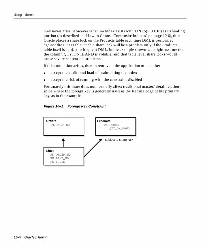
Using Indexes
may never arise. However when no index exists with LINES(PCODE) as its leadingportion (as described in "How to Choose Composite Indexes" on page 10-6), thenOracle places a share lock on the Products table each time DML is performedagainst the Lines table. Such a share lock will be a problem only if the Productstable itself is subject to frequent DML. In the example shown we might assume thatthe column QTY_ON_HAND is volatile, and that table level share locks wouldcause severe contention problems.
If this contention arises, then to remove it the application must either
■ accept the additional load of maintaining the index
■ accept the risk of running with the constraint disabled
Fortunately this issue does not normally affect traditional master/detail relation-ships where the foreign key is generally used as the leading edge of the primarykey, as in the example.
Figure 10–1 Foreign Key Constraint
subject to share lock
BuildLinesPK ORDER_NOPK LINE_NOFK PCODE
ProductsPK PCODE QTY_ON_HAND
Design
OrdersPK ORDR_NO
10-4 Oracle8 Tuning
Using Indexes
How to Choose Columns to IndexFollow these guidelines for choosing columns to index:
■ Consider indexing columns that are used frequently in WHERE clauses.
■ Consider indexing columns that are used frequently to join tables in SQL state-ments. For more information on optimizing joins, see the section "How to Use aHash Cluster" on page 10-26.
■ Only index columns with good selectivity. The selectivity of an index is the per-centage of rows in a table having the same value for the indexed column. Anindex’s selectivity is good if few rows have the same value.
Note: Oracle implicitly creates indexes on the columns of all unique and pri-mary keys that you define with integrity constraints. These indexes are themost selective and the most effective in optimizing performance.
You can determine the selectivity of an index by dividing the number of rowsin the table by the number of distinct indexed values. You can obtain these val-ues using the ANALYZE command. Selectivity calculated in this mannershould be interpreted as a percentage.
■ Do not use standard B*-tree indexes on columns with few distinct values. Suchcolumns usually have poor selectivity and, therefore, do not optimize perfor-mance unless the frequently selected column values appear less frequentlythan the other column values. You can use bitmap indexes effectively in suchcases, unless a high concurrency OLTP application is involved.
■ Do not index columns that are frequently modified. UPDATE statements thatmodify indexed columns and INSERT and DELETE statements that modifyindexed tables take longer than if there were no index. Such SQL statementsmust modify data in indexes as well as data in tables. They also generate addi-tional undo and redo information.
■ Do not index columns that appear only in WHERE clauses with functions oroperators. A WHERE clause that uses a function (other than MIN or MAX) oran operator with an indexed column does not make available the access paththat uses the index.
■ Consider indexing foreign keys of referential integrity constraints in cases inwhich a large number of concurrent INSERT, UPDATE, and DELETE state-ments access the parent and child tables. With UPDATE and DELETE, such anindex allows Oracle to modify data in the child table without locking the par-ent table.
Data Access Methods 10-5
Using Indexes
■ When choosing whether to index a column, consider whether the performancegain for queries is worth the performance loss for INSERT, UPDATE, andDELETE statements and the use of the space required to store the index. Youmay want to experiment and compare the processing times of your SQL state-ments with and without indexes. You can measure processing time with theSQL trace facility.
See Also: Chapter 24, “The SQL Trace Facility and TKPROF”Oracle8 Concepts regarding the effects of foreign keys on locking
How to Choose Composite IndexesA composite index contains more than one key column. Composite indexes can pro-vide additional advantages over single-column indexes:
A SQL statement can use an access path involving a composite index if the state-ment contains constructs that use a leading portion of the index. A leading portionof an index is a set of one or more columns that were specified first and consecu-tively in the list of columns in the CREATE INDEX statement that created theindex. Consider this CREATE INDEX statement:
CREATE INDEX comp_ind ON tab1(x, y, z);
These combinations of columns are leading portions of the index: X, XY, and XYZ.These combinations of columns are not leading portions of the index: YZ and Z.
Follow these guidelines for choosing columns for composite indexes:
■ Consider creating a composite index on columns that are frequently usedtogether in WHERE clause conditions combined with AND operators, espe-cially if their combined selectivity is better than the selectivity of either columnindividually.
■ If several queries select the same set of columns based on one or more columnvalues, consider creating a composite index containing all of these columns.
better selectivity Sometimes two or more columns, each with poor selec-tivity, can be combined to form a composite index withgood selectivity.
additional data storage If all the columns selected by a query are in a compositeindex, Oracle can return these values from the indexwithout accessing the table.
10-6 Oracle8 Tuning
Using Indexes
Of course, consider the guidelines associated with the general performance advan-tages and trade-offs of indexes described in the previous sections. Follow theseguidelines for ordering columns in composite indexes:
■ Create the index so that the columns that are used in WHERE clauses make upa leading portion.
■ If some of the columns are used in WHERE clauses more frequently, be sure tocreate the index so that the more frequently selected columns make up a lead-ing portion to allow the statements that use only these columns to use theindex.
■ If all columns are used in WHERE clauses equally often, ordering these col-umns from most selective to least selective in the CREATE INDEX statementbest improves query performance.
■ If all columns are used in the WHERE clauses equally often but the data isphysically ordered on one of the columns, place that column first in the com-posite index.
How to Write Statements that Use IndexesEven after you create an index, the optimizer cannot use an access path that usesthe index simply because the index exists. The optimizer can choose such an accesspath for a SQL statement only if it contains a construct that makes the access pathavailable.
To be sure that a SQL statement can use an access path that uses an index, be surethe statement contains a construct that makes such an access path available. If youare using the cost-based approach, you should also generate statistics for the index.Once you have made the access path available for the statement, the optimizer mayor may not choose to use the access path, based on the availability of other accesspaths.
If you create new indexes to tune statements, you can also use the EXPLAIN PLANcommand to determine whether the optimizer will choose to use these indexeswhen the application is run. If you create new indexes to tune a statement that iscurrently parsed, Oracle invalidates the statement. When the statement is next exe-cuted, the optimizer automatically chooses a new execution plan that could poten-tially use the new index. If you create new indexes on a remote database to tune adistributed statement, the optimizer considers these indexes when the statement isnext parsed.
Also keep in mind that the means you use to tune one statement may affect theoptimizer’s choice of execution plans for others. For example, if you create an index
Data Access Methods 10-7
Using Indexes
to be used by one statement, the optimizer may choose to use that index for otherstatements in your application as well. For this reason, you should re-examine yourapplication’s performance and rerun the SQL trace facility after you have tunedthose statements that you initially identified for tuning.
How to Write Statements that Avoid Using IndexesIn some cases, you may want to prevent a SQL statement from using an access paththat uses an existing index. You may want to do this if you know that the index isnot very selective and that a full table scan would be more efficient. If the statementcontains a construct that makes such an index access path available, you can forcethe optimizer to use a full table scan through one of these methods:
■ You can make the index access path unavailable by modifying the statement ina way that does not change its meaning.
■ You can use the FULL hint to force the optimizer to choose a full table scaninstead of an index scan.
■ You can use the INDEX or AND_EQUAL hint to force the optimizer to use oneindex or set of indexes instead of another.
The behavior of the optimizer may change in future versions of Oracle, so relyingon methods such as the first to choose access paths may not be a good long-rangeplan. Instead, use hints to suggest specific access paths to the optimizer.
Assessing the Value of IndexesA crude way to determine whether an index is good is to create it, analyze it, anduse EXPLAIN PLAN on your query to see if the optimizer uses it. If it does, keepthe index unless it is very expensive to maintain. This method, however, is verytime and resource expensive. A preferable method is to compare the optimizer cost(in the first row of EXPLAIN PLAN output) of the plans with and without theindex.
The parallel query feature utilizes indexes effectively. It does not perform parallelindex range scans, but it does perform parallel index lookups for parallel nestedloop join execution. If an index is very selective (there are few rows per indexentry), then it may be better to use sequential index lookup than parallel table scan.
10-8 Oracle8 Tuning
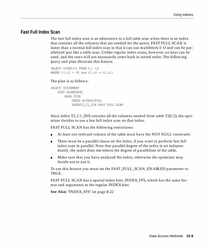
Using Indexes
Fast Full Index ScanThe fast full index scan is an alternative to a full table scan when there is an indexthat contains all the columns that are needed for the query. FAST FULL SCAN isfaster than a normal full index scan in that it can use multiblock I/O and can be par-allelized just like a table scan. Unlike regular index scans, however, no keys can beused, and the rows will not necessarily come back in sorted order. The followingquery and plan illustrate this feature.
SELECT COUNT(*) FROM t1, t2WHERE t1.c1 > 50 and t1.c2 = t2.c1;
The plan is as follows:
SELECT STATEMENTSORT AGGREGATE
HASH JOINTABLE ACCESS1FULLINDEXT2_C1_IDX FAST FULL SCAN
Since index T2_C1_IDX contains all the columns needed from table T2(C2), the opti-mizer decides to use a fast full index scan on that index.
FAST FULL SCAN has the following restrictions:
■ At least one indexed column of the table must have the NOT NULL constraint.
■ There must be a parallel clause on the index, if you want to perform fast fullindex scan in parallel. Note that parallel degree of the index is set indepen-dently: the index does not inherit the degree of parallelism of the table.
■ Make sure that you have analyzed the index, otherwise the optimizer maydecide not to use it.
To use this feature you must set the FAST_FULL_SCAN_ENABLED parameter toTRUE.
FAST FULL SCAN has a special index hint, INDEX_FFS, which has the same for-mat and arguments as the regular INDEX hint.
See Also: "INDEX_FFS" on page 8-22
Data Access Methods 10-9
Using Indexes
Re-creating an IndexYou may wish to re-create an index in order to compact it and clean up fragmentedspace, or to change the index’s storage characteristics. When creating a new indexthat is a subset of an existing index, or when rebuilding an existing index with newstorage characteristics, Oracle uses the existing index instead of the base table toimprove performance.
Consider, for example, a table named CUST with columns NAME, CUSTID,PHONE, ADDR, BALANCE, and an index named I_CUST_CUSTINFO on table col-umns NAME, CUSTID and BALANCE. To create a new index namedI_CUST_CUSTNO on columns CUSTID and NAME, you would enter:
CREATE INDEX I_CUST_CUSTNO on CUST(CUSTID,NAME);
Oracle automatically uses the existing index (I_CUST_CUSTINFO) to create thenew index rather than accessing the entire table. Note that the syntax used is thesame as if the index I_CUST_CUSTINFO did not exist.
Similarly, if you have an index on the EMPNO and MGR columns of the EMP table,and you want to change the storage characteristics of that composite index, Oraclecan use the existing index to create the new index.
Use the ALTER INDEX ... REBUILD statement to reorganize or compact an existingindex or to change its storage characteristics. The REBUILD uses the existing indexas the basis for the new index. All index storage commands are supported, such asSTORAGE (for extent allocation), TABLESPACE (to move the index to a newtablespace), and INITRANS (to change the initial number of entries).
ALTER INDEX ... REBUILD is usually faster than dropping and re-creating anindex, because it utilizes the fast full scan feature. It thus reads all the index blocksusing multiblock I/O, then discards the branch blocks. A further advantage of thisapproach is that the old index is still available for queries (but not for DML) whilethe rebuild is in progress.
See Also: Oracle8 SQL Reference for more information about the CREATE INDEXand ALTER INDEX commands.
10-10 Oracle8 Tuning
Using Indexes
Using Existing Indexes to Enforce UniquenessYou can use an existing index on a table to enforce uniqueness, either for UNIQUEconstraints or the unique aspect of a PRIMARY KEY constraint. The advantage ofthis approach is that the index remains available and valid when the constraint isdisabled. Therefore, enabling a disabled UNIQUE or PRIMARY KEY constraintdoes not require that you rebuild the unique index associated with the constraint.This can yield significant time savings on enable operations for large tables.
Using a nonunique index to enforce uniqueness also allows you to eliminate redun-dant indexes. You do not need a unique index on a primary key column if that col-umn already is included as the prefix of a composite index. The existing index canbe used to enable and enforce the constraint and you can save significant space bynot duplicating the index.
Nonunique indexes also have significant advantages when enabling enforced con-straints (described in the next section). If you use a nonunique index to enforce aUNIQUE constraint, then when you change the constraint from disabled toenforced, you do not need to rebuild the constraint's index. The existing index isused and the enable operation happens very quickly.
Using Enforced ConstraintsAn enforced constraint behaves similarly to an enabled constraint. Placing a con-straint in the enforced state signifies that any new data entered into the table mustconform to the constraint. Existing data is not checked. Placing a constraint in theenforced state allows you to enable the constraint without locking the table.
If you change an enforced constraint from disabled to enabled, the table must belocked. No new DML, queries, or DDL can occur, because no mechanism exists toensure that operations on the table conform to the constraint during the enableoperation. The enforced state ensures that no operation violating the constraint canbe performed upon the table. Therefore, a constraint can go from enabled toenforced with a parallel, consistent-read query of the table to determine whetherany data violates the constraint. No locking is performed, and the enable operationdoes not block readers or writers to the table. In addition, enforced constraints canbe enabled in parallel: multiple constraints can be enabled at the same time, andeach constraint's validity check can performed using parallel query processors.
Data Access Methods 10-11
Using Indexes
The best approach to creating a table with integrity constraints is as follows:
1. For UNIQUE or PRIMARY KEY constraints, create the table with the con-straints disabled. For all other constraints, create the table with the constraintsenabled.
2. For UNIQUE or PRIMARY KEY constraints, create a nonunique index on theUNIQUE or PRIMARY KEY columns.
3. For UNIQUE or PRIMARY KEY constraints, enable the constraints.
4. Begin entering data into the table.
5. During an IMPORT or load operation, you may wish to disable the constraintfor faster processing.
6. Immediately after the IMPORT or load, place the constraint into theENFORCED state.
7. After enforcing the constraint, perform an ALTER TABLE ... ENABLE CON-STRAINT operation for all of the constraints on the table.
Constraints can be created as enforced. Disabled constraints can be made enforcedwith the statement
ALTER TABLE tablename ENFORCE CONSTRAINT constraint;
This statement is about as fast as ALTER TABLE tablename DISABLE, since bothstatements lock the table but need not check anything.
The IMPORT utility automatically enforces, then enables, named constraints. Itenables constraints more slowly if the name is system generated.
See Also: Oracle8 Concepts for a complete discussion of integrity constraints.
10-12 Oracle8 Tuning

Using Bitmap Indexes
Using Bitmap IndexesThis section describes:
■ When to Use Bitmap Indexing
■ How to Create a Bitmap Index
■ Initialization Parameters for Bitmap Indexing
■ Using Bitmap Access Plans on Regular B*-tree Indexes
■ Estimating Bitmap Index Size
■ Bitmap Index Restrictions
See Also: Oracle8 Concepts, for a general introduction to bitmap indexing.
When to Use Bitmap IndexingThis section describes three aspects of the indexing scheme you must evaluatewhen considering whether to use bitmap indexing on a given table: performance,storage, and maintenance.
Performance ConsiderationsBitmap indexes can substantially improve performance of queries with the follow-ing characteristics:
■ The WHERE clause contains multiple predicates on low- or medium-cardinal-ity columns.
■ The individual predicates on these low- or medium-cardinality columns selecta large number of rows.
■ Bitmap indexes have been created on some or all of these low- or medium-car-dinality columns.
■ The tables being queried contain many rows.
You can use multiple bitmap indexes to evaluate the conditions on a single table.Bitmap indexes are thus highly advantageous for complex ad hoc queries that con-tain lengthy WHERE clauses. Bitmap indexes can also provide optimal perfor-mance for aggregate queries.
Data Access Methods 10-13
Using Bitmap Indexes
Storage ConsiderationsBitmap indexes can provide considerable storage savings over the use of multicol-umn (or concatenated) B*-tree indexes. In databases that contain only B*-treeindexes, a DBA must anticipate the columns that would commonly be accessedtogether in a single query, and create a composite B*-tree index on these columns.Not only would this B*-tree index require a large amount of space, but it wouldalso be ordered. That is, a B*-tree index on (MARITAL_STATUS, REGION, GEN-DER) is useless for a query that only accesses REGION and GENDER. To com-pletely index the database, the DBA would have to create indexes on the otherpermutations of these columns. For the simple case of three low-cardinality col-umns, there are six possible composite B*-tree indexes. DBAs must consider thetrade-offs between disk space and performance needs when determining whichcomposite B*-tree indexes to create.
Bitmap indexes solve this dilemma. Bitmap indexes can be efficiently combinedduring query execution, so three small single-column bitmap indexes can do thejob of six three-column B*-tree indexes. Although the bitmap indexes may not bequite as efficient during execution as the appropriate composite B*-tree indexes, thespace savings more than justifies their use.
If a bitmap index is created on a unique key column, it requires more space than aregular B*-tree index. However, for columns where each value is repeated hun-dreds or thousands of times, a bitmap index typically is less than 25% of the size ofa regular B*-tree index. The bitmaps themselves are stored in compressed format.
Simply comparing the relative sizes of B*-tree and bitmap indexes is not an accu-rate measure of effectiveness, however. Because of their different performance char-acteristics, you should keep B*-tree indexes on high-cardinality data, while creatingbitmap indexes on low-cardinality data.
10-14 Oracle8 Tuning
Using Bitmap Indexes
Maintenance ConsiderationsBitmap indexes benefit data warehousing applications, but are not appropriate forOLTP applications with a heavy load of concurrent insert, update, and delete opera-tions. In a data warehousing environment, data is usually maintained by way ofbulk inserts and updates. Index maintenance is deferred until the end of each DMLoperation. For example, if you insert 1000 rows, the inserted rows are all placedinto a sort buffer and then the updates of all 1000 index entries are batched. (This iswhy SORT_AREA_SIZE must be set properly for good performance with insertsand updates on bitmap indexes.) Thus each bitmap segment is updated only onceper DML operation, even if more than one row in that segment changes.
Note: The sorts described above are regular sorts and use the regular sort area,determined by SORT_AREA_SIZE. The BITMAP_MERGE_AREA_SIZE andCREATE_BITMAP_AREA_SIZE parameters described in "Initialization Parametersfor Bitmap Indexing" on page 10-18 only affect the specific operations indicated bythe parameter names.
DML and DDL statements such as UPDATE, DELETE, DROP TABLE, and so on,affect bitmap indexes the same way they do traditional indexes: the consistencymodel is the same. A compressed bitmap for a key value is made up of one or morebitmap segments, each of which is at most half a block in size (but may be smaller).The locking granularity is one such bitmap segment. This may affect performancein environments where many transactions make simultaneous updates. If numer-ous DML operations have caused increased index size and decreasing performancefor queries, you can use the ALTER INDEX ... REBUILD command to compact theindex and restore efficient performance.
A B*-tree index entry contains a single ROWID. Therefore, when the index entry islocked, a single row is locked. With bitmap indexes, an entry can potentially con-tain a range of ROWIDs. When a bitmap index entry is locked, the entire range ofROWIDs is locked. The number of ROWIDs in this range affects concurrency. Forexample, a bitmap index on a column with unique values would lock one ROWIDper value: concurrency would be the same as for B*-tree indexes. As ROWIDsincrease in a bitmap segment, concurrency decreases.
Locking issues affect DML operations, and thus may affect heavy OLTP environ-ments. Locking issues do not, however, affect query performance. As with othertypes of indexes, updating bitmap indexes is a costly operation. Nonetheless, forbulk inserts and updates where many rows are inserted or many updates are madein a single statement, performance with bitmap indexes can be better than with reg-ular B*-tree indexes.
Data Access Methods 10-15
Using Bitmap Indexes
How to Create a Bitmap IndexTo create a bitmap index, use the BITMAP keyword in the CREATE INDEX com-mand:
CREATE BITMAP INDEX ...
All CREATE INDEX parameters except NOSORT are applicable to bitmap indexes.Multi-column (concatenated) bitmap indexes are supported; they can be definedover at most 30 columns. Other SQL statements concerning indexes, such as DROP,ANALYZE, ALTER, and so on, can refer to bitmap indexes without any extra key-word.
Note: The COMPATIBLE initialization parameter must be set to 7.3.2 or higher, forbitmap indexing to be available.
Index TypeSystem index views USER_INDEXES, ALL_INDEXES, and DBA_INDEXES indi-cate bitmap indexes by the word BITMAP appearing in the TYPE column. A bit-map index cannot be declared as UNIQUE.
Using HintsThe INDEX hint works with bitmap indexes in the same way as with traditionalindexes.
The INDEX_COMBINE hint indicates to the optimizer the indexes that are costeffective to use. The optimizer recognizes all indexes that can potentially be com-bined, given the predicates in the WHERE clause. However, it may not be cost effec-tive to use all of them.
In deciding which of them actually to use, the optimizer includes nonhintedindexes that look cost effective as well as indexes that are named in the hint. If cer-tain indexes are given as arguments for the hint, the optimizer tries to use somecombination of those particular bitmap indexes.
If no indexes are named in the hint, all indexes are considered hinted. Hence, theoptimizer will try to combine as many as is possible given the WHERE clause, with-out regard to cost effectiveness. The optimizer always tries to use hinted indexes inthe plan, whether or not it considers them cost effective.
See Also: "INDEX_COMBINE" on page 8-21
10-16 Oracle8 Tuning
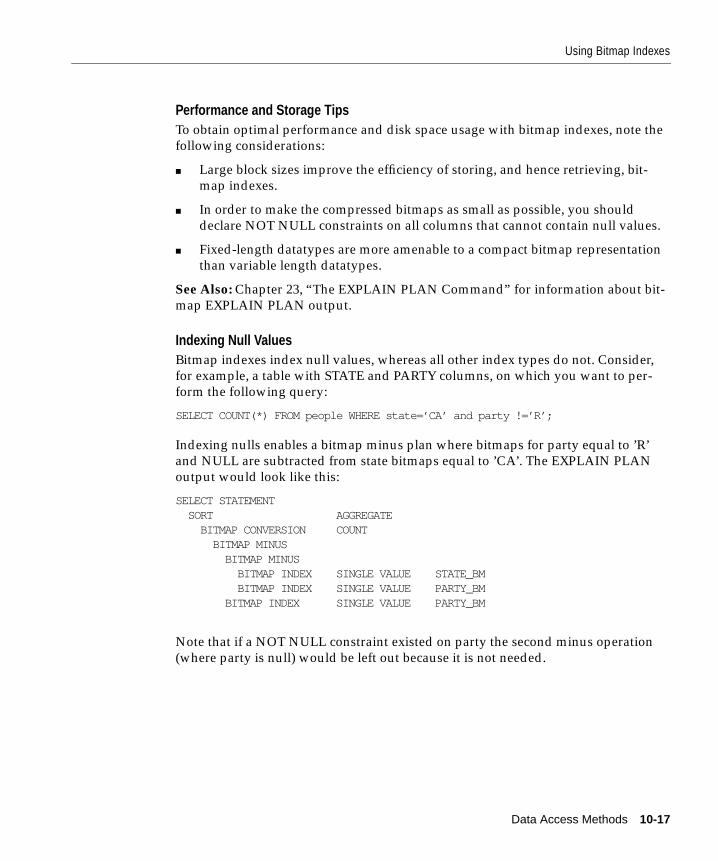
Using Bitmap Indexes
Performance and Storage TipsTo obtain optimal performance and disk space usage with bitmap indexes, note thefollowing considerations:
■ Large block sizes improve the efficiency of storing, and hence retrieving, bit-map indexes.
■ In order to make the compressed bitmaps as small as possible, you shoulddeclare NOT NULL constraints on all columns that cannot contain null values.
■ Fixed-length datatypes are more amenable to a compact bitmap representationthan variable length datatypes.
See Also: Chapter 23, “The EXPLAIN PLAN Command” for information about bit-map EXPLAIN PLAN output.
Indexing Null ValuesBitmap indexes index null values, whereas all other index types do not. Consider,for example, a table with STATE and PARTY columns, on which you want to per-form the following query:
SELECT COUNT(*) FROM people WHERE state=’CA’ and party !=’R’;
Indexing nulls enables a bitmap minus plan where bitmaps for party equal to ’R’and NULL are subtracted from state bitmaps equal to ’CA’. The EXPLAIN PLANoutput would look like this:
SELECT STATEMENT SORT AGGREGATE BITMAP CONVERSION COUNT BITMAP MINUS BITMAP MINUS BITMAP INDEX SINGLE VALUE STATE_BM BITMAP INDEX SINGLE VALUE PARTY_BM BITMAP INDEX SINGLE VALUE PARTY_BM
Note that if a NOT NULL constraint existed on party the second minus operation(where party is null) would be left out because it is not needed.
Data Access Methods 10-17
Using Bitmap Indexes
Initialization Parameters for Bitmap IndexingThe following two initialization parameters have an impact on performance.
CREATE_BITMAP_AREA_SIZEThis parameter determines the amount of memory allocated for bitmap creation.The default value is 8 Mb. A larger value may lead to faster index creation. If cardi-nality is very small, you can set a small value for this parameter. For example, if car-dinality is only 2, then the value can be on the order of kilobytes rather thanmegabytes. As a general rule, the higher the cardinality, the more memory isneeded for optimal performance. This parameter is not dynamically alterable at thesession level.
BITMAP_MERGE_AREA_SIZEThis parameter determines the amount of memory used to merge bitmapsretrieved from a range scan of the index. The default value is 1 Mb. A larger valueshould improve performance, because the bitmap segments must be sorted beforebeing merged into a single bitmap. This parameter is not dynamically alterable atthe session level.
10-18 Oracle8 Tuning
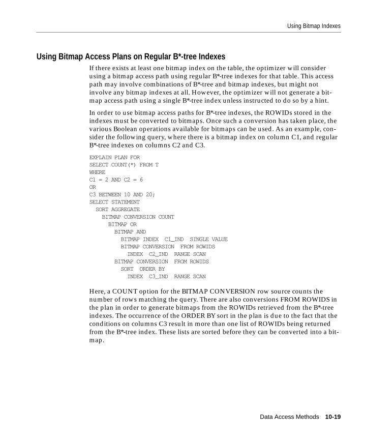
Using Bitmap Indexes
Using Bitmap Access Plans on Regular B*-tree IndexesIf there exists at least one bitmap index on the table, the optimizer will considerusing a bitmap access path using regular B*-tree indexes for that table. This accesspath may involve combinations of B*-tree and bitmap indexes, but might notinvolve any bitmap indexes at all. However, the optimizer will not generate a bit-map access path using a single B*-tree index unless instructed to do so by a hint.
In order to use bitmap access paths for B*-tree indexes, the ROWIDs stored in theindexes must be converted to bitmaps. Once such a conversion has taken place, thevarious Boolean operations available for bitmaps can be used. As an example, con-sider the following query, where there is a bitmap index on column C1, and regularB*-tree indexes on columns C2 and C3.
EXPLAIN PLAN FORSELECT COUNT(*) FROM TWHEREC1 = 2 AND C2 = 6ORC3 BETWEEN 10 AND 20;SELECT STATEMENT SORT AGGREGATE BITMAP CONVERSION COUNT BITMAP OR BITMAP AND BITMAP INDEX C1_IND SINGLE VALUE BITMAP CONVERSION FROM ROWIDS INDEX C2_IND RANGE SCAN BITMAP CONVERSION FROM ROWIDS SORT ORDER BY INDEX C3_IND RANGE SCAN
Here, a COUNT option for the BITMAP CONVERSION row source counts thenumber of rows matching the query. There are also conversions FROM ROWIDS inthe plan in order to generate bitmaps from the ROWIDs retrieved from the B*-treeindexes. The occurrence of the ORDER BY sort in the plan is due to the fact that theconditions on columns C3 result in more than one list of ROWIDs being returnedfrom the B*-tree index. These lists are sorted before they can be converted into a bit-map.
Data Access Methods 10-19
Using Bitmap Indexes
Estimating Bitmap Index SizeAlthough it is not possible to size a bitmap index exactly, you can estimate its size.This section describes how to extrapolate the size of a bitmap index for a table fromthe computed size of a B*-tree index. It also illustrates how cardinality, NOT NULLconstraints and number of distinct values, affects bitmap size.
To estimate the size of a bitmap index for a given table, you may extrapolate fromthe size of a B*-tree index for the table. Use the following approach:
1. Use the standard formula described in Oracle8 Concepts to compute the size of aB*-tree index for the table.
2. Determine the cardinality of the table data.
3. From the cardinality value, extrapolate the size of a bitmap index according tothe graph in Figure 10–2 or Figure 10–3.
For a 1 million row table, Figure 10–2 shows index size on columns with differentnumbers of distinct values, for B*-tree indexes and bitmap indexes. UsingFigure 10–2 you can estimate the size of a bitmap index relative to that of a B*-treeindex for the table. Sizing is not exact: results will vary somewhat from table totable.
Note that randomly distributed data was used to generate the graph. If, in yourdata, particular values tend to cluster close together, you may generate consider-ably smaller bitmap indexes than indicated by the graph. Bitmap indexes may beslightly smaller than those in the graph if columns contain NOT NULL constraints.
Figure 10–3 shows similar data for a table with 5 million rows. Note that when car-dinality exceeds 100,000, bitmap index size does not increase as fast as it does inFigure 10–2. For a table with more rows, there are more repeating values for a givencardinality.
10-20 Oracle8 Tuning
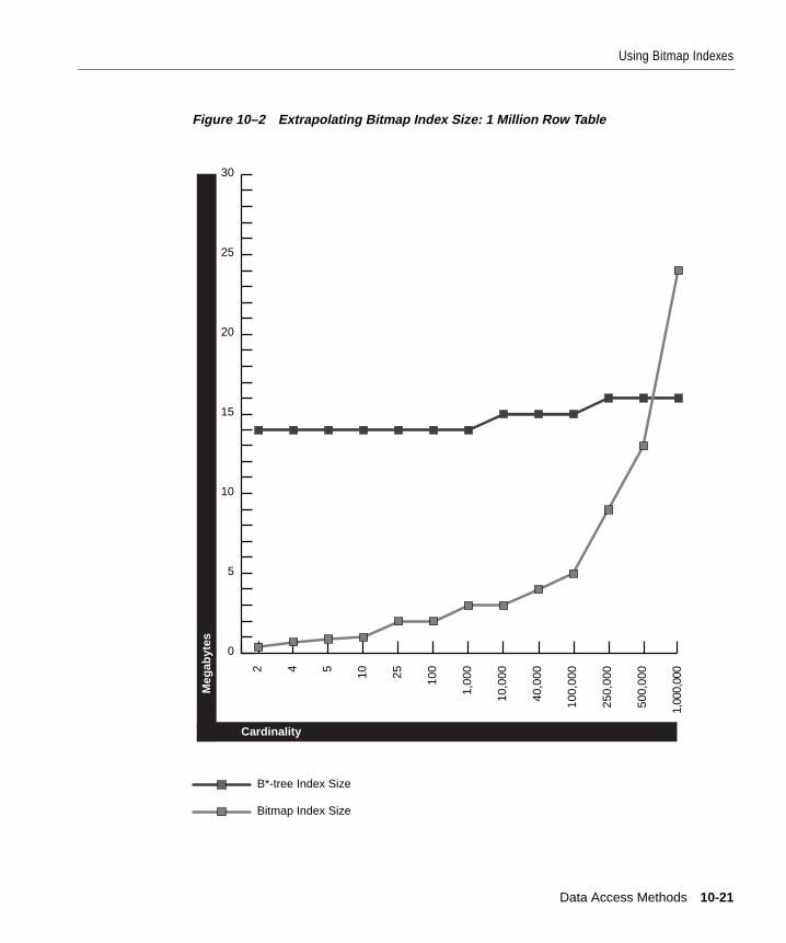
Using Bitmap Indexes
Figure 10–2 Extrapolating Bitmap Index Size: 1 Million Row Table
0
5
10
15
20
25
30
B*-tree Index Size
Bitmap Index Size
1,00
0,00
0
500,
000
250,
000
100,
000
40,0
00
10,0
00
1,00
0
1002510542
Meg
abyt
es
Cardinality
Data Access Methods 10-21
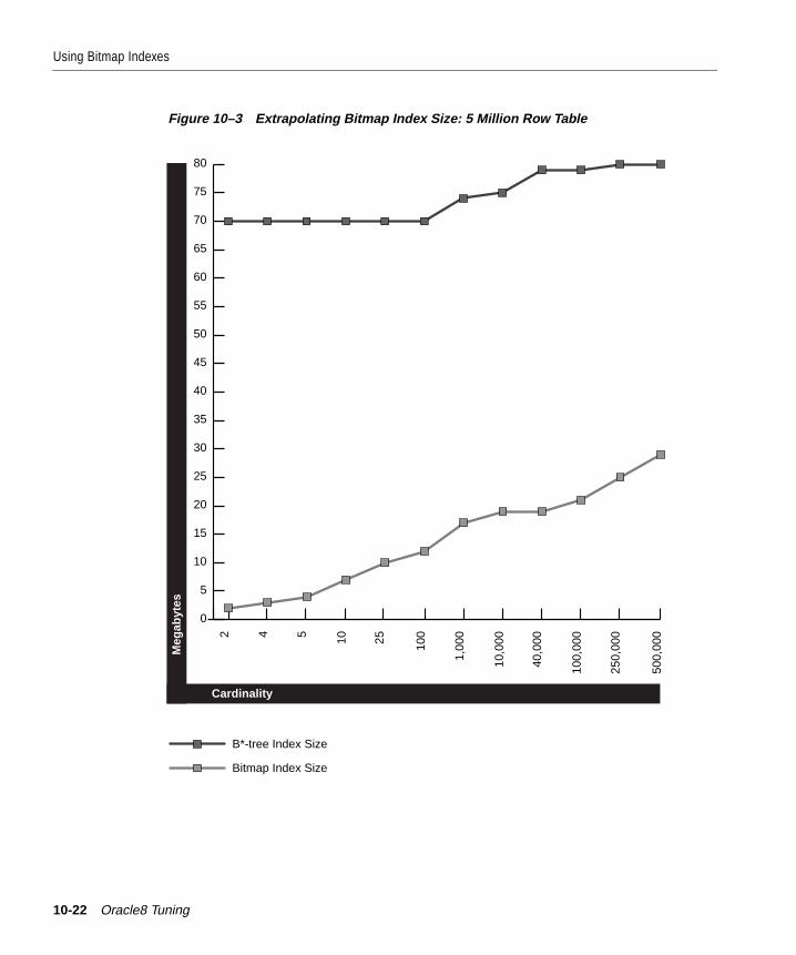
Using Bitmap Indexes
Figure 10–3 Extrapolating Bitmap Index Size: 5 Million Row Table
500,
000
250,
000
100,
000
40,0
00
10,0
00
1,00
0
1002510542
0
5
10
15
20
25
30
35
40
45
50
55
60
65
70
75
80
B*-tree Index Size
Bitmap Index Size
Meg
abyt
es
Cardinality
10-22 Oracle8 Tuning
Using Bitmap Indexes
Bitmap Index RestrictionsBitmap indexes have the following restrictions:
■ For bitmap indexes with direct load, the SORTED_INDEX flag does not apply.
■ Performing an ALTER TABLE command that adds or modifies a bitmap-indexed column may cause indexes to be invalidated.
■ Bitmap indexes are not considered by the rule-based optimizer.
■ Bitmap indexes cannot be used for referential integrity checking.
Data Access Methods 10-23
Using Clusters
Using ClustersFollow these guidelines when deciding whether to cluster tables:
■ Consider clustering tables that are often accessed by your application in joinstatements.
■ Do not cluster tables if your application joins them only occasionally or modi-fies their common column values frequently. Modifying a row’s cluster keyvalue takes longer than modifying the value in an unclustered table, becauseOracle may have to migrate the modified row to another block to maintain thecluster.
■ Do not cluster tables if your application often performs full table scans of onlyone of the tables. A full table scan of a clustered table can take longer than a fulltable scan of an unclustered table. Oracle is likely to read more blocks becausethe tables are stored together.
■ Consider clustering master-detail tables if you often select a master record andthen the corresponding detail records. Detail records are stored in the samedata block(s) as the master record, so they are likely still to be in memory whenyou select them, requiring Oracle to perform less I/O.
■ Consider storing a detail table alone in a cluster if you often select many detailrecords of the same master. This measure improves the performance of queriesthat select detail records of the same master but does not decrease the perfor-mance of a full table scan on the master table.
■ Do not cluster tables if the data from all tables with the same cluster key valueexceeds more than one or two Oracle blocks. To access a row in a clusteredtable, Oracle reads all blocks containing rows with that value. If these rowstake up multiple blocks, accessing a single row could require more reads thanaccessing the same row in an unclustered table.
Consider the benefits and drawbacks of clusters with respect to the needs of yourapplication. For example, you may decide that the performance gain for join state-ments outweighs the performance loss for statements that modify cluster key val-ues. You may want to experiment and compare processing times with your tablesboth clustered and stored separately. To create a cluster, use the CREATE CLUSTERcommand.
See Also: For more information on creating clusters, see the Oracle8 ApplicationDeveloper’s Guide.
10-24 Oracle8 Tuning
Using Hash Clusters
Using Hash ClustersHash clusters group table data by applying a hash function to each row’s clusterkey value. All rows with the same cluster key value are stored together on disk.Consider the benefits and drawbacks of hash clusters with respect to the needs ofyour application. You may want to experiment and compare processing times witha particular table as it is stored in a hash cluster, and as it is stored alone with anindex. This section describes:
■ When to Use a Hash Cluster
■ How to Use a Hash Cluster
When to Use a Hash ClusterFollow these guidelines for choosing when to use hash clusters:
■ Consider using hash clusters to store tables that are often accessed by SQL state-ments with WHERE clauses if the WHERE clauses contain equality conditionsthat use the same column or combination of columns. Designate this column orcombination of columns as the cluster key.
■ Store a table in a hash cluster if you can determine how much space is requiredto hold all rows with a given cluster key value, including rows to be insertedimmediately as well as rows to be inserted in the future.
■ Do not use hash clusters if space in your database is scarce and you cannotafford to allocate additional space for rows to be inserted in the future.
■ Do not use a hash cluster to store a constantly growing table if the process ofoccasionally creating a new, larger hash cluster to hold that table is impractical.
■ Do not store a table in a hash cluster if your application often performs fulltable scans and you must allocate a great deal of space to the hash cluster inanticipation of the table growing. Such full table scans must read all blocks allo-cated to the hash cluster, even though some blocks may contain few rows. Stor-ing the table alone would reduce the number of blocks read by full table scans.
■ Do not store a table in a hash cluster if your application frequently modifies thecluster key values. Modifying a row’s cluster key value can take longer thanmodifying the value in an unclustered table, because Oracle may have tomigrate the modified row to another block to maintain the cluster.
■ Storing a single table in a hash cluster can be useful, regardless of whether thetable is often joined with other tables, provided that hashing is appropriate forthe table based on the previous points in this list.
Data Access Methods 10-25
Using Hash Clusters
How to Use a Hash ClusterTo create a hash cluster, use the CREATE CLUSTER command with the HASH andHASHKEYS parameters.
When you create a hash cluster, you must use the HASHKEYS parameter of theCREATE CLUSTER statement to specify the number of hash values for the hashcluster. For best performance of hash scans, choose a HASHKEYS value that is atleast as large as the number of cluster key values. Such a value reduces the chanceof collisions, or multiple cluster key values resulting in the same hash value. Colli-sions force Oracle to test the rows in each block for the correct cluster key valueafter performing a hash scan. Collisions reduce the performance of hash scans.
Oracle always rounds up the HASHKEYS value that you specify to the nearestprime number to obtain the actual number of hash values. This rounding isdesigned to reduce collisions.
See Also: For more information on creating hash clusters, see the Oracle8 Applica-tion Developer’s Guide.
10-26 Oracle8 Tuning
Oracle8 Transaction M
11
Oracle8 Transaction ModesThis chapter describes the different modes in which read consistency is performed.Topics in this chapter include:
■ Using Discrete Transactions
■ Using Serializable Transactions
odes 11-1
Using Discrete Transactions
Using Discrete TransactionsYou can improve the performance of short, nondistributed transactions by usingthe BEGIN_DISCRETE_TRANSACTION procedure. This procedure streamlinestransaction processing so short transactions can execute more rapidly. This sectiondescribes:
■ Deciding When to Use Discrete Transactions
■ How Discrete Transactions Work
■ Errors During Discrete Transactions
■ Usage Notes
■ Example
Deciding When to Use Discrete TransactionsDiscrete transaction processing is useful for transactions that:
■ modify only a few database blocks
■ never change an individual database block more than once per transaction
■ do not modify data likely to be requested by long-running queries
■ do not need to see the new value of data after modifying the data
■ do not modify tables containing any LONG values
In deciding to use discrete transactions, you should consider the following factors:
■ Can the transaction be designed to work within the constraints placed on dis-crete transactions, as described in "Usage Notes" on page 11-4?
■ Does using discrete transactions result in a significant performance improve-ment under normal usage conditions?
Discrete transactions can be used concurrently with standard transactions. Choos-ing whether to use discrete transactions should be a part of your normal tuning pro-cedure. Although discrete transactions can be used only for a subset of alltransactions, for sophisticated users with advanced application requirements,where speed is the most critical factor, the performance improvements can makeworking within the design constraints worthwhile.
11-2 Oracle8 Tuning
Using Discrete Transactions
How Discrete Transactions WorkDuring a discrete transaction, all changes made to any data are deferred until thetransaction commits. Redo information is generated, but is stored in a separate loca-tion in memory.
When the transaction issues a commit request, the redo information is written tothe redo log file (along with other group commits) and the changes to the databaseblock are applied directly to the block. The block is written to the database file inthe usual manner. Control is returned to the application once the commit com-pletes. This eliminates the need to generate undo information, because the block isnot actually modified until the transaction is committed, and the redo informationis stored in the redo log buffers.
As with other transactions, the uncommitted changes of a discrete transaction arenot visible to concurrent transactions. For regular transactions, undo information isused to re-create old versions of data for queries that require a consistent view ofthe data. Because no undo information is generated for discrete transactions, a dis-crete transaction that starts and completes during a long query can cause the queryto receive the “snapshot too old” error if the query requests data changed by thediscrete transaction. For this reason, you might want to avoid performing queriesthat access a large subset of a table that is modified by frequent discrete transac-tions.
To use the BEGIN_DISCRETE_TRANSACTION procedure, theDISCRETE_TRANSACTIONS_ENABLED initialization parameter must be set toTRUE. If this parameter is set to FALSE, all calls toBEGIN_DISCRETE_TRANSACTION are ignored and transactions requesting thisservice are handled as standard transactions.
See Also: Oracle8 Reference for information about setting initialization parameters.
Errors During Discrete TransactionsAny errors encountered during processing of a discrete transaction cause the pre-defined exception DISCRETE_TRANSACTION_FAILED to be raised. These errorsinclude the failure of a discrete transaction to comply with the usage notes outlinedbelow. (For example, calling BEGIN_DISCRETE_TRANSACTION after a transac-tion has begun, or attempting to modify the same database block more than onceduring a transaction, raises the exception.)
Oracle8 Transaction Modes 11-3
Using Discrete Transactions
Usage NotesThe BEGIN_DISCRETE_TRANSACTION procedure must be called before the firststatement in a transaction. This call to the procedure is effective only for the dura-tion of the transaction (that is, once the transaction is committed or rolled back, thenext transaction is processed as a standard transaction).
Transactions that use this procedure cannot participate in distributed transactions.
Although discrete transactions cannot see their own changes, you can obtain theold value and lock the row, using the FOR UPDATE clause of the SELECT state-ment, before updating the value.
Because discrete transactions cannot see their own changes, a discrete transactioncannot perform inserts or updates on both tables involved in a referential integrityconstraint.
For example, assume the EMP table has a FOREIGN KEY constraint on theDEPTNO column that refers to the DEPT table. A discrete transaction cannotattempt to add a department into the DEPT table and then add an employeebelonging to that department, because the department is not added to the tableuntil the transaction commits and the integrity constraint requires that the depart-ment exist before an insert into the EMP table can occur. These two operations mustbe performed in separate discrete transactions.
Because discrete transactions can change each database block only once, some com-binations of data manipulation statements on the same table are better suited fordiscrete transactions than others. One INSERT statement and one UPDATE state-ment used together are the least likely to affect the same block. Multiple UPDATEstatements are also unlikely to affect the same block, depending on the size of theaffected tables. Multiple INSERT statements (or INSERT statements that use que-ries to specify values), however, are likely to affect the same database block. Multi-ple DML operations performed on separate tables do not affect the same databaseblocks, unless the tables are clustered.
ExampleAn application for checking out library books is an example of a transaction typethat uses the BEGIN_DISCRETE_TRANSACTION procedure. The following proce-dure is called by the library application with the book number as the argument.This procedure checks to see if the book is reserved before allowing it to be checkedout. If more copies of the book have been reserved than are available, the statusRES is returned to the library application, which calls another procedure to reservethe book, if desired. Otherwise, the book is checked out and the inventory of booksavailable is updated.
11-4 Oracle8 Tuning
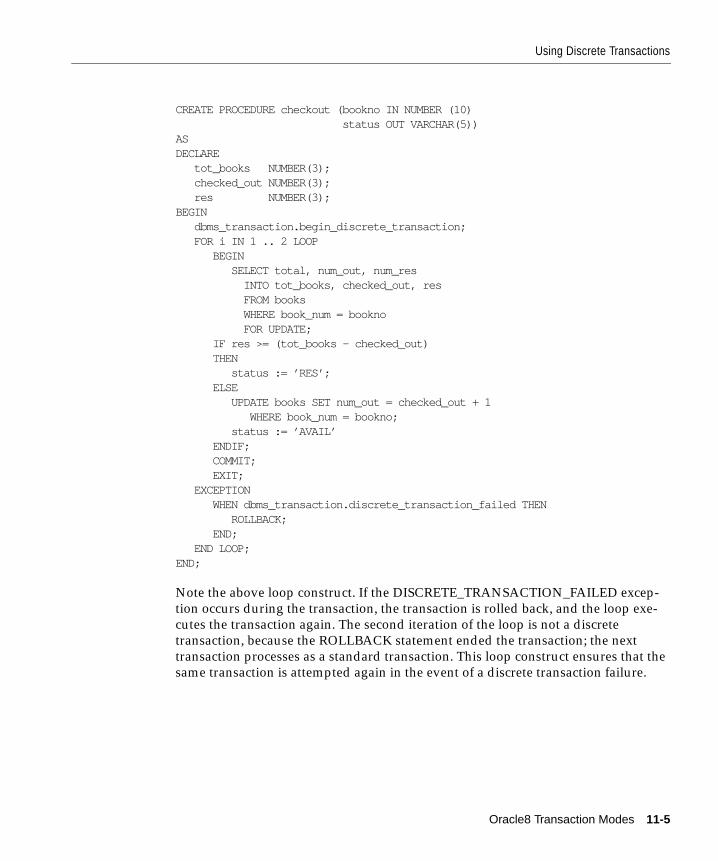
Using Discrete Transactions
CREATE PROCEDURE checkout (bookno IN NUMBER (10) status OUT VARCHAR(5))ASDECLARE tot_books NUMBER(3); checked_out NUMBER(3); res NUMBER(3);BEGIN dbms_transaction.begin_discrete_transaction; FOR i IN 1 .. 2 LOOP BEGIN SELECT total, num_out, num_res INTO tot_books, checked_out, res FROM books WHERE book_num = bookno FOR UPDATE; IF res >= (tot_books - checked_out) THEN status := ’RES’; ELSE UPDATE books SET num_out = checked_out + 1 WHERE book_num = bookno; status := ’AVAIL’ ENDIF; COMMIT; EXIT; EXCEPTION WHEN dbms_transaction.discrete_transaction_failed THEN ROLLBACK; END; END LOOP;END;
Note the above loop construct. If the DISCRETE_TRANSACTION_FAILED excep-tion occurs during the transaction, the transaction is rolled back, and the loop exe-cutes the transaction again. The second iteration of the loop is not a discretetransaction, because the ROLLBACK statement ended the transaction; the nexttransaction processes as a standard transaction. This loop construct ensures that thesame transaction is attempted again in the event of a discrete transaction failure.
Oracle8 Transaction Modes 11-5
Using Serializable Transactions
Using Serializable TransactionsOracle allows application developers to set the isolation level of transactions. Theisolation level determines what changes the transaction and other transactions cansee. The ISO/ANSI SQL3 specification details the following levels of transactionisolation.
If you wish to set the transaction isolation level, you must do so before the transac-tion begins. Use the SET TRANSACTION ISOLATION LEVEL statement for a par-ticular transaction, or the ALTER SESSION SET ISOLATION_LEVEL statement forall subsequent transactions in the session.
See Also: Oracle8 SQL Reference for more information on the syntax of SET TRANS-ACTION and ALTER SESSION.
SERIALIZABLE Transactions lose no updates, provide repeatable reads,and do not experience phantoms. Changes made to aserializable transaction are visible only to the transac-tion itself.
READ COMMITTED Transactions do not have repeatable reads and changesmade in this transaction or other transactions are visibleto all transactions. This is the default transaction isola-tion.
11-6 Oracle8 Tuning
Managing SQL and Shared PL/SQL
12
Managing SQL and Shared PL/SQL AreasThis chapter explains the use of shared SQL to improve performance. Topics in thischapter include
■ Introduction
■ Comparing SQL Statements and PL/SQL Blocks
■ Keeping Shared SQL and PL/SQL in the Shared Pool
Areas 12-1
Introduction
IntroductionOracle compares SQL statements and PL/SQL blocks issued directly by users andapplications as well as recursive SQL statements issued internally by a DDL state-ment. If two identical statements are issued, the SQL or PL/SQL area used to pro-cess the first instance of the statement is shared, or used for the processing of thesubsequent executions of that same statement.
Shared SQL and PL/SQL areas are shared memory areas; any Oracle process canuse a shared SQL area. The use of shared SQL areas reduces memory usage on thedatabase server, thereby increasing system throughput.
Shared SQL and PL/SQL areas are aged out of the shared pool by way of a leastrecently used algorithm (similar to database buffers). To improve performance andprevent reparsing, you may want to prevent large SQL or PL/SQL areas fromaging out of the shared pool.
Comparing SQL Statements and PL/SQL BlocksThis section describes
■ Testing for Identical SQL Statements
■ Aspects of Standardized SQL Formatting
12-2 Oracle8 Tuning
Comparing SQL Statements and PL/SQL Blocks
Testing for Identical SQL StatementsOracle automatically notices when two or more applications send identical SQLstatements or PL/SQL blocks to the database. It does not have to parse a statementto determine whether it is identical to another statement currently in the sharedpool. Oracle distinguishes identical statements using the following steps:
1. The text string of an issued statement is hashed. If the hash value is the same asa hash value for an existing SQL statement in the shared pool, Oracle proceedsto Step 2.
2. The text string of the issued statement, including case, blanks, and comments,is compared to all existing SQL statements that were identified in Step 1.
3. The objects referenced in the issued statement are compared to the referencedobjects of all existing statements identified in Step 2. For example, if two usershave EMP tables, the statement
SELECT * FROM emp;
is not considered identical because the statement references different tables foreach user.
4. The bind types of bind variables used in a SQL statement must match.
Note: Most Oracle products convert the SQL before passing statements to the data-base. Characters are uniformly changed to upper case, white space is compressed,and bind variables are renamed so that a consistent set of SQL statements is pro-duced.
Aspects of Standardized SQL FormattingIt is neither necessary nor useful to have every user of an application attempt towrite SQL statements in a standardized way. It is unlikely that 300 people writingad hoc dynamic statements in standardized SQL will generate the same SQL state-ments. The chances that they will all want to look at exactly the same columns inexactly the same tables in exactly the same order is quite remote. By contrast, 300people running the same application—executing command files—will generate thesame SQL statements.
Within an application there is a very minimal advantage to having 2 statementsalmost the same, and 300 users using them; there is a major advantage to havingone statement used by 600 users.
Managing SQL and Shared PL/SQL Areas 12-3
Keeping Shared SQL and PL/SQL in the Shared Pool
Keeping Shared SQL and PL/SQL in the Shared PoolThis section describes two techniques of keeping shared SQL and PL/SQL in theshared pool:
■ Reserving Space for Large Allocations
■ Preventing Objects from Being Aged Out
Reserving Space for Large AllocationsA problem can occur if users fill the shared pool, and then a large package ages out.If someone should then call the large package back in, an enormous amount ofmaintenance must be done to create space for it in the shared pool. You can avoidthis problem by reserving space for large allocations with theSHARED_POOL_RESERVED_SIZE initialization parameter. This parameter setsaside room in the shared pool for allocations larger than the value specified by theSHARED_POOL_RESERVED_SIZE_MIN_ALLOC parameter.
Note: Although Oracle8 uses segmented codes to reduce the need for large areas ofcontiguous memory, it may still be valuable for performance reasons for you to pinlarge objects in memory.
Preventing Objects from Being Aged OutThe DBMS_SHARED_POOL package lets you keep objects in shared memory, sothat they will not be aged out with the normal LRU mechanism. The DBM-SPOOL.SQL and PRVTPOOL.PLB procedure scripts create the package specifica-tion and package body for DBMS_SHARED_POOL.
By using the DBMS_SHARED_POOL package and by loading early these SQL andPL/SQL areas (before memory fragmentation occurs), the objects can be kept inmemory, instead of aging out with the normal LRU mechanism. This procedureensures that memory is available and prevents sudden, seemingly inexplicableslowdowns in user response time that occur when SQL and PL/SQL areas areaccessed after aging out.
12-4 Oracle8 Tuning
Keeping Shared SQL and PL/SQL in the Shared Pool
When to Use DBMS_SHARED_POOLThe procedures provided with the DBMS_SHARED_POOL package may be usefulwhen loading large PL/SQL objects, such as the STANDARD and DIUTIL pack-ages.
When large PL/SQL objects are loaded, users’ response time is affected because ofthe large number of smaller objects that need to be aged out from the shared poolto make room (due to memory fragmentation). In some cases, there may be insuffi-cient memory to load the large objects.
DBMS_SHARED_POOL is also useful for frequently executed triggers. You maywant to keep compiled triggers on frequently used tables in the shared pool.
Note in addition that DBMS_SHARED_POOL supports sequences. Sequence num-bers are lost when a sequence is aged out of the shared pool.DBMS_SHARED_POOL is useful for keeping sequences in the shared pool andthus preventing the loss of sequence numbers.
Managing SQL and Shared PL/SQL Areas 12-5
Keeping Shared SQL and PL/SQL in the Shared Pool
How to Use DBMS_SHARED_POOLTo use the DBMS_SHARED_POOL package to pin a SQL or PL/SQL area, com-plete the following steps.
1. Decide which packages/cursors you would like pinned in memory.
2. Start up the database.
3. Make the call to DBMS_SHARED_POOL.KEEP to pin it.
This procedure ensures that your system does not run out of the shared memorybefore the object is loaded. Finally, by pinning the object early in the life of theinstance, this procedure prevents the memory fragmentation that could result frompinning a large chunk of memory in the middle of the shared pool.
The procedures provided with the DBMS_SHARED_POOL package are describedbelow.
DBMS_SHARED_POOL.SIZESThis procedure shows the objects in the shared pool that are larger than the speci-fied size.
dbms_shared_pool.sizes(minsize IN NUMBER)
Input Parameter:
To display the results of this procedure, before calling this procedure issue the fol-lowing command using Server Manager or SQL*Plus:
SET SERVEROUTPUT ON SIZE minsize
You can use the results of this command as arguments to the KEEP or UNKEEP pro-cedures.
For example, to show the objects in the shared pool that are larger than 2000 kilo-bytes, issue the following Server Manager or SQL*Plus commands:
SQL> SET SERVEROUTPUT ON SIZE 2000SQL> EXECUTE DBMS_SHARED_POOL.SIZES(2000);
minsize Display objects in shared pool larger than this size, wheresize is measured in kilobytes.
12-6 Oracle8 Tuning
Keeping Shared SQL and PL/SQL in the Shared Pool
DBMS_SHARED_POOL.KEEPThis procedure lets you keep an object in the shared pool. This procedure may notbe supported in future releases.
dbms_shared_pool.keep(object IN VARCHAR2, [type IN CHAR DEFAULT P])
Input Parameters:
DBMS_SHARED_POOL.UNKEEPThis procedure allows an object that you have requested to be kept in the sharedpool now to be aged out of the shared pool.
Note: This procedure may not be supported in the future.
dbms_shared_pool.unkeep(object IN VARCHAR2, [type IN CHAR DEFAULT P])
Input Parameters:
object Either the parameter name or the cursor address of the object to bekept in the shared pool. This is the value displayed when you callthe SIZES procedure.
type The type of the object to be kept in the shared pool. Types include:
P procedure
C cursor
R trigger
Q sequence
object Either the parameter name or the cursor address of the object thatyou no longer want kept in the shared pool. This is the value dis-played when you call the SIZES procedure.
type Type of the object to be aged out of the shared pool. Types include:
P procedure
C cursor
R trigger
Q sequence
Managing SQL and Shared PL/SQL Areas 12-7

Keeping Shared SQL and PL/SQL in the Shared Pool
12-8 Oracle8 Tuning
Part IV
Optimizing Oracle Instance PerformancesPart IV describes how to tune various elements of your database system in order tooptimize performance of an Oracle instance. The chapters are:
■ Chapter 13, “Tuning CPU Resources”
■ Chapter 14, “Tuning Memory Allocation”
■ Chapter 15, “Tuning I/O”
■ Chapter 16, “Tuning Networks”
■ Chapter 17, “Tuning the Operating System”
■ Chapter 18, “Tuning Resource Contention”

Tuning CPU Reso
13
Tuning CPU ResourcesThis chapter describes how to identify and solve problems with central processingunit (CPU) resources. Topics in this chapter include
■ Understanding CPU Problems
■ How to Detect and Solve CPU Problems
■ Solving CPU Problems by Changing System Architecture
urces 13-1
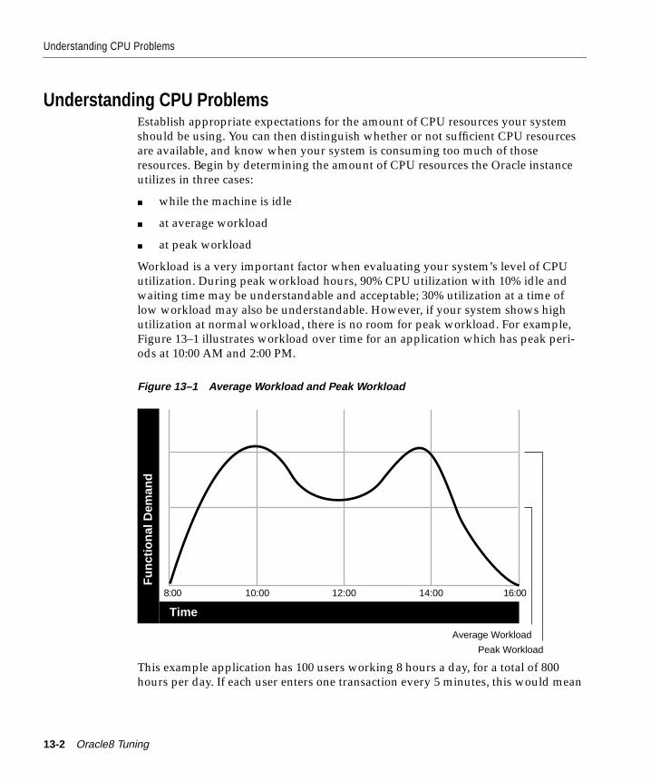
Understanding CPU Problems
Understanding CPU ProblemsEstablish appropriate expectations for the amount of CPU resources your systemshould be using. You can then distinguish whether or not sufficient CPU resourcesare available, and know when your system is consuming too much of thoseresources. Begin by determining the amount of CPU resources the Oracle instanceutilizes in three cases:
■ while the machine is idle
■ at average workload
■ at peak workload
Workload is a very important factor when evaluating your system’s level of CPUutilization. During peak workload hours, 90% CPU utilization with 10% idle andwaiting time may be understandable and acceptable; 30% utilization at a time oflow workload may also be understandable. However, if your system shows highutilization at normal workload, there is no room for peak workload. For example,Figure 13–1 illustrates workload over time for an application which has peak peri-ods at 10:00 AM and 2:00 PM.
Figure 13–1 Average Workload and Peak Workload
This example application has 100 users working 8 hours a day, for a total of 800hours per day. If each user enters one transaction every 5 minutes, this would mean
Time
Fu
nct
ion
al D
eman
d
8:00 10:00 12:00 14:00 16:00
Peak Workload
Average Workload
13-2 Oracle8 Tuning
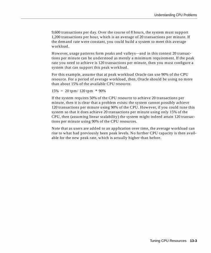
Understanding CPU Problems
9,600 transactions per day. Over the course of 8 hours, the system must support1,200 transactions per hour, which is an average of 20 transactions per minute. Ifthe demand rate were constant, you could build a system to meet this averageworkload.
However, usage patterns form peaks and valleys—and in this context 20 transac-tions per minute can be understood as merely a minimum requirement. If the peakrate you need to achieve is 120 transactions per minute, then you must configure asystem that can support this peak workload.
For this example, assume that at peak workload Oracle can use 90% of the CPUresource. For a period of average workload, then, Oracle should be using no morethan about 15% of the available CPU resource.
15% = 20 tpm/120 tpm * 90%
If the system requires 50% of the CPU resource to achieve 20 transactions perminute, then it is clear that a problem exists: the system cannot possibly achieve120 transactions per minute using 90% of the CPU. However, if you could tune thissystem so that it does achieve 20 transactions per minute using only 15% of theCPU, then (assuming linear scalability) the system might indeed attain 120 transac-tions per minute using 90% of the CPU resources.
Note that as users are added to an application over time, the average workload canrise to what had previously been peak levels. No further CPU capacity is then avail-able for the new peak rate, which is actually higher than before.
Tuning CPU Resources 13-3
How to Detect and Solve CPU Problems
How to Detect and Solve CPU ProblemsIf you suspect a problem with CPU usage, you must evaluate two areas:
■ Checking System CPU Utilization
■ Checking Oracle CPU Utilization
Checking System CPU UtilizationOracle statistics report CPU utilization only of Oracle sessions, whereas every pro-cess running on your system affects the available CPU resources. Effort spent tun-ing non-Oracle factors can thus result in better Oracle performance.
Use operating system monitoring tools to see what processes are running on thesystem as a whole. If the system is too heavily loaded, check the memory, I/O, andprocess management areas described later in this section.
Tools such as sar -u on many UNIX-based systems enable you to examine the levelof CPU utilization on your entire system. CPU utilization in UNIX is described instatistics that show user time, system time, idle time, and time waiting for I/O. ACPU problem exists if idle time and time waiting for I/O are both close to zero (lessthan 5%) at a normal or low workload.
Performance Monitor is used on NT systems to examine CPU utilization. It pro-vides statistics on processor time, user time, privileged time, interrupt time, andDPC time. (NT Performance Monitor is not the same as Performance Manager,which is an Oracle Enterprise Manager tool.)
Attention: This section describes how to check system CPU utilization on mostUNIX-based and NT systems. For other platforms, please check your operating sys-tem documentation.
Memory ManagementCheck the following memory management issues:
Paging and Swapping. Use the appropriate tools (such as sar or vmstat on UNIXor Performance Monitor on NT) to investigate the cause of paging and swapping,should they occur.
Oversize Page Tables. On UNIX systems, if the processing space becomes toolarge, it may result in the page tables becoming too large. This is not an issue on NTsystems.
13-4 Oracle8 Tuning
How to Detect and Solve CPU Problems
I/O ManagementCheck the following I/O management issues:
Thrashing. Make sure that your workloads fits in memory so that the machine isnot thrashing (swapping and paging processes in and out of memory). The operat-ing system allocates fixed slices of time during which CPU resources are availableto your process. If the process squanders a large portion of each time slice checkingto be sure that it can run, that all needed components are in the machine, it may beusing only 50% of the time allotted to actually perform work.
Client/Server Round Trips. The latency of sending a message may result in CPUoverload. An application often generates messages that need to be sent through thenetwork over and over again. This results in a lot of overhead that must be com-pleted before the message is actually sent. To alleviate this problem you can batchthe messages and perform the overhead only once, or reduce the amount of work.For example, you can use array inserts, array fetches, and so on.
Process ManagementCheck the following process management issues:
Scheduling and Switching. The operating system may spend a lot of time in sched-uling and switching processes. Examine the way in which you are using the operat-ing system: you could be using too many processes. On NT systems, do notoverload your server with a great deal of non-Oracle processes.
Context Switching. Due to operating system specific characteristics, your systemcould be spending a lot of time in context switches. This could be expensive, espe-cially with a very large SGA. Note that context switching is not an issue on NT,which has only one process per instance; all threads share the same page table.
Programmers often create single-purpose processes on the fly; then they exit theprocess, and create a new one so that the process is re-created and destroyed all thetime. This is very CPU intensive, especially with large SGAs, because you have tobuild up the page tables each time. The problem is aggravated when you nail orlock shared memory, because you have to touch every page.
For example, if you have a 1 gigabyte SGA, you may have page table entries forevery 4K, and a page table entry may be 8 bytes. You could end up with(1G /4K) * 8B entries. This becomes expensive, because you have to continuallymake sure that the page table is loaded.
Parallel query and multithreaded server are areas of concern here if MINSERVICEhas been set too low (set to 10, for example, when you need 20).
Tuning CPU Resources 13-5
How to Detect and Solve CPU Problems
For the user, doing small lookups may not be wise. In a situation like this, itbecomes inefficient for the user and for the system as well.
Checking Oracle CPU UtilizationThis section explains how to examine the processes running in Oracle. Twodynamic performance views provide information on Oracle processes:
■ V$SYSSTAT shows Oracle CPU usage for all sessions. The statistic “CPU usedby this session” actually shows the aggregate CPU used by all sessions.
■ V$SESSTAT shows Oracle CPU usage per session. You can use this view to seewhich particular session is using the most CPU.
For example, if you have 8 CPUs, then for any given minute in real time, you have8 minutes of CPU time available. On NT and UNIX-based systems this can beeither user time or time in system mode (“privileged” mode, in NT). If your pro-cess is not running, it is waiting. CPU time utilized by all systems may thus begreater than one minute per interval.
At any given moment you know how much time Oracle has utilized the system. Soif 8 minutes are available and Oracle uses 4 minutes of that time, then you knowthat 50% of all CPU time is used by Oracle. If your process is not consuming thattime, then some other process is. Go back to the system and find out what processis using up the CPU time. Identify the process, determine why it is using so muchCPU time, and see if you can tune it.
The major areas to check for Oracle CPU utilization are:
■ Reparsing SQL Statements
■ Inefficient SQL Statements
■ Read Consistency
■ Scalability Limitations within the Application
■ Latch Contention
This section describes each area, and indicates the corresponding Oracle statisticsto check.
13-6 Oracle8 Tuning
How to Detect and Solve CPU Problems
Reparsing SQL StatementsIneffective SQL sharing can result in reparsing.
1. Begin by checking V$SYSSTAT to see if parsing in general is a problem:
SELECT * FROM V$SYSSTATWHERE NAME IN(’parse time cpu’, ’parse time elapsed’, ’parse count (hard)’);
In interpreting these statistics, remember
■ response time = service time + wait time, therefore response time = elapsedtime
■ service time = CPU time, therefore elapsed time - CPU time = wait time
In this way you can detect the general response time on parsing. The moreyour application is parsing, the more contention exists and the more time youwill spend waiting. Note that
■ wait time/parse count = average wait time per parse
■ The average wait time should be extremely low, approaching zero.(V$SYSSTAT also indicates the average wait time per parse.)
2. Next, query V$SQLAREA to find frequently reparsed statements:
SELECT SQL_TEXT, PARSE_CALLS, EXECUTIONS FROM V$SQLAREAORDER BY PARSE_CALLS;
3. Now that you have identified problematic statements, you have the followingthree options for tuning them:
■ Rewrite the application so statements do not continually reparse.
■ If this is not possible, reduce parsing by using the initialization parameterSESSION_CACHED_CURSORS.
■ If the parse count is small, the execute count is small, and the SQL state-ments are very similar except for the WHERE clause, you may find thathard coded values are being used instead of bind variables. Change to bindvariables in order to reduce parsing.
Tuning CPU Resources 13-7
How to Detect and Solve CPU Problems
Inefficient SQL StatementsInefficient SQL statements can consume large amounts of CPU resource. To detectsuch statements, enter the following query. You may be able to reduce CPU usageby tuning SQL statements that have a high number of buffer gets.
SELECT BUFFER_GETS, EXECUTIONS, SQL_TEXT FROM V$SQLAREA;
See Also: "Approaches to SQL Statement Tuning" on page 7-6
Read ConsistencyYour system could spend a lot of time rolling back changes to blocks in order tomaintain a consistent view.
■ If there are many small transactions and an active long-running query is run-ning in the background on the same table where the inserts are happening, thequery may have to roll back many changes.
■ If the number of rollback segments is too small, your system could also bespending a lot of time rolling back the transaction table. Your query may havestarted long ago; because the number of rollback segments and transactiontables is very small, your system frequently needs to reuse transaction slots.
A solution is to make more rollback segments, or to increase the commit rate.For example, if you batch ten transactions and commit them once, you reducethe number of transactions by a factor of ten.
■ If your system has to scan too many buffers in the foreground to find a freebuffer, it wastes CPU resources. To alleviate this problem, tune the DBWn pro-cess(es) to write more frequently.
You can also increase the size of the buffer cache to enable the database writerprocess(es) to keep up. To find the average number of buffers the system scansat the end of the least recently used list (LRU) to find a free buffer, use the fol-lowing formula:
Normally you would expect to see 1 or 2 buffers scanned, on average. If morethan this number are being scanned, increase the size of the buffer cache ortune the DBWn process(es).
inspected”= avg. buffers scanned
1 + value of "free buffers inspected"
"free buffers inspected"
13-8 Oracle8 Tuning
How to Detect and Solve CPU Problems
You can apply the following formula to find the number of buffers that weredirty at the end of the LRU:
If many dirty buffers exist, it could mean that the DBWn process(es) cannotkeep up. Again, increase buffer cache size or tune DBWn.
Scalability Limitations Within the ApplicationIn most of this CPU tuning discussion we assume linear scalability, but this is neveractually the case. How flat or nonlinear the scalability is indicates how far awayfrom the ideal you are. Problems in your application might be hurting scalability:examples include too many indexes, right-hand index problems, too much data inblocks, or not partitioning the data. Contention problems like these waste CPUcycles and prevent the application from attaining linear scalability.
Latch ContentionLatch contention is a symptom; it is not normally the cause of CPU problems. Yourtask is to translate the latch contention to an application area: track down the con-tention to determine which part of your application is poorly written.
The spin count may be set too high. Some other process may be holding a latch thatyour process is attempting to get, and your process may be spinning and spinningin an effort to get the latch. After a while your process may go to sleep before wak-ing up to repeat its ineffectual spinning.
■ Check the Oracle latch statistics. The “latch free” event in V$SYSTEM_EVENTshows how long you have been waiting on latches. If there is no latch conten-tion, this statistic will not appear.
■ Check the value of the SPINCOUNT initialization parameter. SPINCOUNTdepends heavily on CPU speed: appropriate values vary significantly from plat-form to platform.
If there is a lot of contention, it may be better for a process to go to sleep at oncewhen it cannot obtain a latch, rather than use up a great deal of CPU time byactively spinning and waiting.
■ Look for the ratio of CPUs to processes. If there are large numbers of both, thenmany process can run. But if a single process is holding a latch on a systemwith ten CPUs, and that process should be rescheduled so that it is not run-
= dirty buffers"dirty buffers inspected"
"free buffers inspected"
Tuning CPU Resources 13-9

Solving CPU Problems by Changing System Architecture
ning, then ten other processes may run ineffectively, trying to get the samelatch. That situation will waste, in parallel, some CPU resource.
■ Check V$LATCH_MISSES, which indicates where in the Oracle code most ofthe contention occurs.
Solving CPU Problems by Changing System ArchitectureIf you have reached the limit of CPU power available on your system, and haveexhausted all means of tuning its CPU usage, then you must consider redesigningyour system. Consider whether moving to a different architecture might result inadequate CPU power. This section describes various possibilities.
■ Single Tier to Two-Tier
■ Multi-Tier: Using Smaller Client Machines
■ Two-Tier to Three-Tier: Using a Transaction Processing Monitor
■ Three-Tier: Using Multiple TP Monitors
■ Oracle Parallel Server
Attention: If you are running a multi-tier system, check all levels for CPU utiliza-tion. For example, on a three-tier system you might learn that your server is mostlyidle and your second tier is completely busy. The solution then would be clear: tunethe second tier, rather than the server or the third tier. In a multi-tier situation, it isusually not the server that has a performance problem: it is usually the clients andthe middle tier.
13-10 Oracle8 Tuning
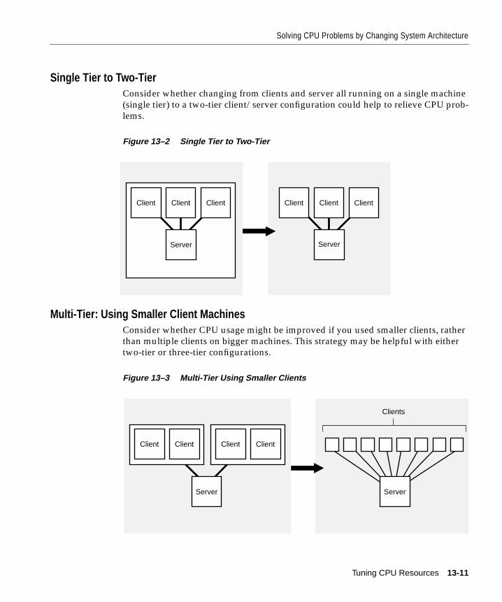
Solving CPU Problems by Changing System Architecture
Single Tier to Two-TierConsider whether changing from clients and server all running on a single machine(single tier) to a two-tier client/server configuration could help to relieve CPU prob-lems.
Figure 13–2 Single Tier to Two-Tier
Multi-Tier: Using Smaller Client MachinesConsider whether CPU usage might be improved if you used smaller clients, ratherthan multiple clients on bigger machines. This strategy may be helpful with eithertwo-tier or three-tier configurations.
Figure 13–3 Multi-Tier Using Smaller Clients
Server
Client Client Client
Server
Client Client Client
ServerServer
Client Client Client Client
Clients
Tuning CPU Resources 13-11
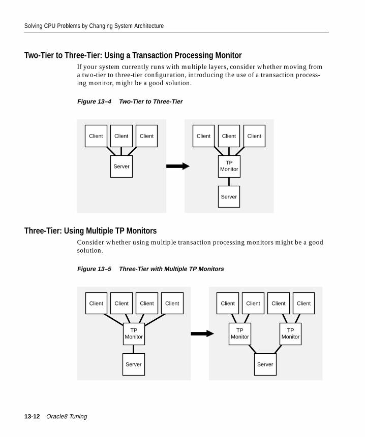
Solving CPU Problems by Changing System Architecture
Two-Tier to Three-Tier: Using a Transaction Processing MonitorIf your system currently runs with multiple layers, consider whether moving froma two-tier to three-tier configuration, introducing the use of a transaction process-ing monitor, might be a good solution.
Figure 13–4 Two-Tier to Three-Tier
Three-Tier: Using Multiple TP MonitorsConsider whether using multiple transaction processing monitors might be a goodsolution.
Figure 13–5 Three-Tier with Multiple TP Monitors
TPMonitor
Client Client
Server
Client
Server
Client Client Client
ClientClientClient Client
Server
Client
Server
TPMonitor
TPMonitor
Client ClientClient
TPMonitor
13-12 Oracle8 Tuning
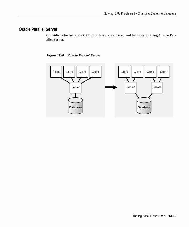
Solving CPU Problems by Changing System Architecture
Oracle Parallel ServerConsider whether your CPU problems could be solved by incorporating Oracle Par-allel Server.
Figure 13–6 Oracle Parallel Server
ClientClientClient ClientClient
ServerServer
Client ClientClient
Server
Database Database
Tuning CPU Resources 13-13

Solving CPU Problems by Changing System Architecture
13-14 Oracle8 Tuning

Tuning Memory Alloc
14
Tuning Memory AllocationThis chapter explains how to allocate memory to database structures. Proper sizingof these structures can greatly improve database performance. The following topicsare covered:
■ Understanding Memory Allocation Issues
■ How to Detect Memory Allocation Problems
■ How to Solve Memory Allocation Problems
■ Tuning Operating System Memory Requirements
■ Tuning the Redo Log Buffer
■ Tuning Private SQL and PL/SQL Areas
■ Tuning the Shared Pool
■ Tuning the Buffer Cache
■ Tuning Multiple Buffer Pools
■ Tuning Sort Areas
■ Reallocating Memory
■ Reducing Total Memory Usage
ation 14-1
Understanding Memory Allocation Issues
Understanding Memory Allocation IssuesOracle stores information in memory and on disk. Memory access is much fasterthan disk access, so it is better for data requests to be satisfied by access to memoryrather than access to disk. For best performance, store as much data as possible inmemory rather than on disk. However, memory resources on your operating sys-tem are likely to be limited. Tuning memory allocation involves distributing avail-able memory to Oracle memory structures.
Oracle’s memory requirements depend on your application; therefore, you shouldtune memory allocation after tuning your application and SQL statements. If youallocate memory before tuning your application and SQL statements, you mayneed to resize some Oracle memory structures to meet the needs of your modifiedstatements and application.
Tune memory allocation before you tune I/O. Allocating memory establishes theamount of I/O necessary for Oracle to operate. This chapter shows you how to allo-cate memory to perform as little I/O as possible.
The following terms are used in this discussion:
See Also: Chapter 15, “Tuning I/O”, shows you how to perform I/O as efficientlyas possible.
block A unit of disk storage. A segment is stored in many blocks.
buffer A container in memory for a block. At any point in time abuffer holds a single block. Over time a buffer may hold dif-ferent blocks, as when a new block is needed an old block isdiscarded and replaced with the new one.
buffer pool A collection of buffers.
cache or buffercache
All buffers and buffer pools.
segment A segment is a set of extents that have been allocated for aspecific type of database object such as a table, index, cluster.
14-2 Oracle8 Tuning
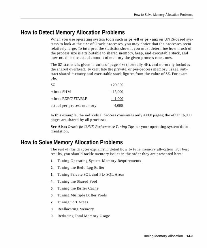
How to Solve Memory Allocation Problems
How to Detect Memory Allocation ProblemsWhen you use operating system tools such as ps -efl or ps - aux on UNIX-based sys-tems to look at the size of Oracle processes, you may notice that the processes seemrelatively large. To interpret the statistics shown, you must determine how much ofthe process size is attributable to shared memory, heap, and executable stack, andhow much is the actual amount of memory the given process consumes.
The SZ statistic is given in units of page size (normally 4K), and normally includesthe shared overhead. To calculate the private, or per-process memory usage, sub-tract shared memory and executable stack figures from the value of SZ. For exam-ple:
In this example, the individual process consumes only 4,000 pages; the other 16,000pages are shared by all processes.
See Also: Oracle for UNIX Performance Tuning Tips, or your operating system docu-mentation.
How to Solve Memory Allocation ProblemsThe rest of this chapter explains in detail how to tune memory allocation. For bestresults, you should tackle memory issues in the order they are presented here:
1. Tuning Operating System Memory Requirements
2. Tuning the Redo Log Buffer
3. Tuning Private SQL and PL/SQL Areas
4. Tuning the Shared Pool
5. Tuning the Buffer Cache
6. Tuning Multiple Buffer Pools
7. Tuning Sort Areas
8. Reallocating Memory
9. Reducing Total Memory Usage
SZ +20,000
minus SHM - 15,000
minus EXECUTABLE - 1,000
actual per-process memory 4,000
Tuning Memory Allocation 14-3
Tuning Operating System Memory Requirements
Tuning Operating System Memory RequirementsBegin tuning memory allocation by tuning your operating system with these goals:
■ Reducing Paging and Swapping
■ Fitting the System Global Area into Main Memory
■ Allocating Enough Memory to Individual Users
These goals apply in general to most operating systems, but the details of operatingsystem tuning vary.
See Also: Refer to your operating system hardware and software documentation aswell as your Oracle operating system-specific documentation for more informationon tuning operating system memory usage.
Reducing Paging and SwappingYour operating system may store information in any of these places:
■ real memory
■ virtual memory
■ expanded storage
■ disk
The operating system may also move information from one storage location toanother, a process known as “paging” or “swapping.” Many operating systemspage and swap to accommodate large amounts of information that do not fit intoreal memory. However, excessive paging or swapping can reduce the performanceof many operating systems.
Monitor your operating system behavior with operating system utilities. Excessivepaging or swapping indicates that new information is often being moved into mem-ory. In this case, your system’s total memory may not be large enough to holdeverything for which you have allocated memory. Either increase the total memoryon your system or decrease the amount of memory you have allocated.
See Also: "Oversubscribe, with Attention to Paging" on page 19-39
14-4 Oracle8 Tuning
Tuning Operating System Memory Requirements
Fitting the System Global Area into Main MemorySince the purpose of the System Global Area (SGA) is to store data in memory forfast access, the SGA should always be contained in main memory. If pages of theSGA are swapped to disk, its data is no longer so quickly accessible. On most oper-ating systems, the disadvantage of excessive paging significantly outweighs theadvantage of a large SGA.
Although it is best to keep the entire SGA in memory, the contents of the SGA willbe split logically between hot and cold parts. The hot parts will always be in mem-ory because they are always being referenced. Some of the cold parts may be pagedout, and a performance penalty may result from bringing them back in. A perfor-mance problem is very likely, however, if the hot part of the SGA cannot stay inmemory.
Remember that data is swapped to disk because it is not being referenced. You cancause Oracle to read the entire SGA into memory when you start your instance bysetting the value of the initialization parameter PRE_PAGE_SGA to YES. Operatingsystem page table entries are then prebuilt for each page of the SGA. This settingmay increase the amount of time necessary for instance startup, but it is likely todecrease the amount of time necessary for Oracle to reach its full performancecapacity after startup. (Note that this setting does not prevent your operating sys-tem from paging or swapping the SGA after it is initially read into memory.)
PRE_PAGE_SGA may also increase the amount of time needed for process startup,because every process that starts must attach to the SGA. The cost of this strategy isfixed, however: you may simply determine that 20,000 pages must be touchedevery time a process is started. This approach may be useful with some applica-tions, but not with all applications. Overhead may be significant if your system cre-ates and destroys processes all the time (by doing continual logon/logoff, forexample).
The advantage that PRE_PAGE_SGA can afford depends on page size. For exam-ple, if the SGA is 80 MB in size, and the page size is 4K, then 20,000 pages must betouched in order to refresh the SGA (80,000/4 = 20,000). If the system permits youto set a 4MB page size, then only 20 pages must be touched to refresh the SGA(80,000/4,000 = 20). Note that the page size is operating-system specific and gener-ally cannot be changed. Some operating systems, however, have a special imple-mentation for shared memory whereby you can change the page size.
You can see how much memory is allocated to the SGA and each of its internalstructures by issuing this Server Manager statement:
SVRMGR> SHOW SGA
Tuning Memory Allocation 14-5
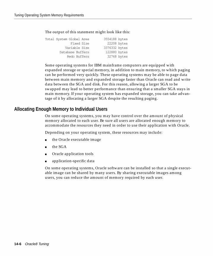
Tuning Operating System Memory Requirements
The output of this statement might look like this:
Total System Global Area 3554188 bytes Fixed Size 22208 bytes Variable Size 3376332 bytes Database Buffers 122880 bytes Redo Buffers 32768 bytes
Some operating systems for IBM mainframe computers are equipped withexpanded storage or special memory, in addition to main memory, to which pagingcan be performed very quickly. These operating systems may be able to page databetween main memory and expanded storage faster than Oracle can read and writedata between the SGA and disk. For this reason, allowing a larger SGA to beswapped may lead to better performance than ensuring that a smaller SGA stays inmain memory. If your operating system has expanded storage, you can take advan-tage of it by allocating a larger SGA despite the resulting paging.
Allocating Enough Memory to Individual UsersOn some operating systems, you may have control over the amount of physicalmemory allocated to each user. Be sure all users are allocated enough memory toaccommodate the resources they need in order to use their application with Oracle.
Depending on your operating system, these resources may include:
■ the Oracle executable image
■ the SGA
■ Oracle application tools
■ application-specific data
On some operating systems, Oracle software can be installed so that a single execut-able image can be shared by many users. By sharing executable images amongusers, you can reduce the amount of memory required by each user.
14-6 Oracle8 Tuning
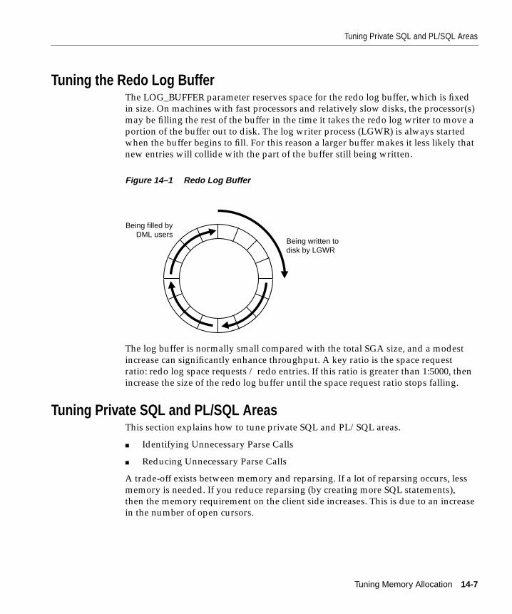
Tuning Private SQL and PL/SQL Areas
Tuning the Redo Log BufferThe LOG_BUFFER parameter reserves space for the redo log buffer, which is fixedin size. On machines with fast processors and relatively slow disks, the processor(s)may be filling the rest of the buffer in the time it takes the redo log writer to move aportion of the buffer out to disk. The log writer process (LGWR) is always startedwhen the buffer begins to fill. For this reason a larger buffer makes it less likely thatnew entries will collide with the part of the buffer still being written.
Figure 14–1 Redo Log Buffer
The log buffer is normally small compared with the total SGA size, and a modestincrease can significantly enhance throughput. A key ratio is the space requestratio: redo log space requests / redo entries. If this ratio is greater than 1:5000, thenincrease the size of the redo log buffer until the space request ratio stops falling.
Tuning Private SQL and PL/SQL AreasThis section explains how to tune private SQL and PL/SQL areas.
■ Identifying Unnecessary Parse Calls
■ Reducing Unnecessary Parse Calls
A trade-off exists between memory and reparsing. If a lot of reparsing occurs, lessmemory is needed. If you reduce reparsing (by creating more SQL statements),then the memory requirement on the client side increases. This is due to an increasein the number of open cursors.
Being written to disk by LGWR
Being filled byDML users
Tuning Memory Allocation 14-7
Tuning Private SQL and PL/SQL Areas
Tuning private SQL areas entails identifying unnecessary parse calls made by yourapplication and then reducing them. To reduce parse calls, you may have toincrease the number of private SQL areas that your application can have allocatedat once. Throughout this section, information about private SQL areas and SQLstatements also applies to private PL/SQL areas and PL/SQL blocks.
Identifying Unnecessary Parse CallsThis section describes three techniques for identifying unnecessary parse calls.
Technique 1One way to identify unnecessary parse calls is to run your application with theSQL trace facility enabled. For each SQL statement in the trace output, the “count”statistic for the Parse step tells you how many times your application makes aparse call for the statement. This statistic includes parse calls that are satisfied byaccess to the library cache as well as parse calls that result in actually parsing thestatement.
Note: This statistic does not include implicit parsing that occurs when an applica-tion executes a statement whose shared SQL area is no longer in the library cache.For information on detecting implicit parsing, see "Examining Library Cache Activ-ity" on page 14-13.
If the “count” value for the Parse step is near the “count” value for the Execute stepfor a statement, your application may be deliberately making a parse call each timeit executes the statement. Try to reduce these parse calls through your applicationtool.
Technique 2Another way to identify unnecessary parse calls is to check the V$SQLAREA view.Enter the following query:
SELECT sql_text, parse_count, executionsFROM V$SQLAREA
When the parse_count value is close to the execution value for a given statement,you may be continually reparsing that particular SQL statement.
Technique 3You can also identify unnecessary parse calls by identifying the session that givesrise to them. It may be that particular batch programs or types of application domost of the reparsing. Execute the following query:
14-8 Oracle8 Tuning
Tuning Private SQL and PL/SQL Areas
SELECT * FROM V$STATNAMEWHERE name in (’parse_count (hard)’,’execute_count’)
The results of the query will look something like this:
statistic#, name------------ ---------100 parse_count90 execute_count
Then run a query like the following:
SELECT * FROM V$SESSTATWHERE statistics# in (90,100)ORDER BY value, sid;
The result will be a list of all sessions and the amount of reparsing they do. Foreach system identifier (sid), go to V$SESSION to find the name of the program thatcauses the reparsing.
Reducing Unnecessary Parse CallsDepending on the Oracle application tool you are using, you may be able to controlhow frequently your application performs parse calls and allocates and deallocatesprivate SQL areas. Whether your application reuses private SQL areas for multipleSQL statements determines how many parse calls your application performs andhow many private SQL areas the application requires.
In general, an application that reuses private SQL areas for multiple SQL state-ments does not need as many private SQL areas as an application that does notreuse private SQL areas. However, an application that reuses private SQL areasmust perform more parse calls, because the application must make a new parse callwhenever an existing private SQL is reused for a new SQL statement.
Be sure that your application can open enough private SQL areas to accommodateall of your SQL statements. If you allocate more private SQL areas, you may needto increase the limit on the number of cursors permitted for a session. You canincrease this limit by increasing the value of the initialization parameterOPEN_CURSORS. The maximum value for this parameter depends on your operat-ing system. The minimum value is 5.
The ways in which you control parse calls and allocation and deallocation of pri-vate SQL areas depends on your Oracle application tool. The following sectionsintroduce the methods used for some tools. Note that these methods apply only toprivate SQL areas and not to shared SQL areas.
Tuning Memory Allocation 14-9
Tuning Private SQL and PL/SQL Areas
Reducing Parse Calls with the Oracle PrecompilersWhen using the Oracle precompilers, you can control private SQL areas and parsecalls by setting three options. In Oracle mode, the options and their defaults are asfollows:
■ HOLD_CURSOR = yes
■ RELEASE_CURSOR = no
■ MAXOPENCURSORS = desired value
Oracle recommends that you not use ANSI mode, in which the values ofHOLD_CURSOR and RELEASE_CURSOR are switched.
The precompiler options can be specified in two ways:
■ on the precompiler command line
■ within the precompiler program
With these options, you can employ different strategies for managing private SQLareas during the course of the program.
See Also: Pro*C/C++ Precompiler Programmer’s Guide for more information on thesecalls
Reducing Parse Calls with Oracle FormsWith Oracle Forms, you also have some control over whether your applicationreuses private SQL areas. You can exercise this control in three places:
■ at the trigger level
■ at the form level
■ at run time
See Also: For more information on the reuse of private SQL areas by Oracle Forms,see the Oracle Forms Reference manual.
14-10 Oracle8 Tuning
Tuning the Shared Pool
Tuning the Shared PoolThis section explains how to allocate memory for key memory structures of theshared pool. Structures are listed in order of importance for tuning.
■ Tuning the Library Cache
■ Tuning the Data Dictionary Cache
■ Tuning the Shared Pool with the Multithreaded Server
■ Tuning Reserved Space from the Shared Pool
Note: If you are using a reserved size for the shared pool, refer to"SHARED_POOL_SIZE Too Small" on page 14-25.
The algorithm that Oracle uses to manage data in the shared pool tends to hold dic-tionary data in memory longer than library cache data. Therefore, tuning thelibrary cache to an acceptable cache hit ratio often ensures that the data dictionarycache hit ratio is also acceptable. Allocating space in the shared pool for sessioninformation is necessary only if you are using the multithreaded server architecture.
In the shared pool, some of the caches are dynamic—they grow or shrink asneeded. These dynamic caches include the library cache and the data dictionarycache. Objects are paged out of these caches if in the shared pool runs out of room.For this reason you may have to increase shared pool size if the “hot” (oftenneeded) set of data does not fit within it. A cache miss on the data dictionary cacheor library cache is more expensive than a miss on the buffer cache. For this reason,you should allocate sufficient memory for the shared pool first.
For most applications, shared pool size is critical to Oracle performance. (Sharedpool size is less important only for applications that issue a very limited number ofdiscrete SQL statements.) The shared pool holds both the data dictionary cache andthe fully parsed or compiled representations of PL/SQL blocks and SQL state-ments. PL/SQL blocks include procedures, functions, packages, triggers and anyanonymous PL/SQL blocks submitted by client-side programs.
If the shared pool is too small, then the server must dedicate resources to managingthe limited space available. This consumes CPU resources and causes contention,because restrictions must be imposed on the parallel management of the variouscaches. The more you use triggers and stored procedures, the larger the shared poolmust be. It may even reach a size measured in hundreds of megabytes.
Because it is better to measure statistics over a specific period rather than from star-tup, you can determine the library cache and row cache (data dictionary cache) hit
Tuning Memory Allocation 14-11
Tuning the Shared Pool
ratios from the following queries. The results show the miss rates for the librarycache and row cache. (In general, the number of reparses reflects the library cache.)
select (sum(pins - reloads)) / sum(pins) "Lib Cache"from v$librarycache;
select (sum(gets - getmisses - usage - fixed)) / sum(gets) "Row Cache"from v$rowcache;
The amount of free memory in the shared pool is reported in V$SGASTAT. Theinstantaneous value can be reported using the query
select * from v$sgastat where name = ’free memory’;
If there is always free memory available within the shared pool, then increasing thesize of the pool will have little or no beneficial effect. However, just because theshared pool is full does not necessarily mean that there is a problem. If the ratiosdiscussed above are close to 1, there is no need to increase the pool size.
Once an entry has been loaded into the shared pool it cannot be moved. As moreentries are loaded, the areas of free memory are broken up and the shared poolmay become fragmented. On UNIX-based systems, you can use the PL/SQL pack-age DBMS_SHARED_POOL, located in dbmspool.sql, to manage the shared pool.The comments in the code describe how to use the procedures within the package.
Oracle8 uses segmented codes to reduce the need for large areas of contiguousmemory. For performance reasons, however, you may still want to pin a largeobject in memory. Using the DBMS_SHARED_POOL package, you can keep largeobjects permanently pinned in the shared pool.
The library cache hit ratio and row cache hit ratio are important. If free memory isclose to zero and either the library cache hit ratio or the row cache hit ratio is lessthan 0.95, then increase the shared pool until the ratios stop improving.
14-12 Oracle8 Tuning
Tuning the Shared Pool
Tuning the Library CacheThe library cache contains shared SQL and PL/SQL areas. This section tells youhow to tune the library cache. Information presented here about shared SQL areasand SQL statements also applies to shared PL/SQL areas and PL/SQL blocks.
Examining Library Cache ActivityLibrary cache misses can occur on either the parse or the execute step in the pro-cessing of a SQL statement.
Parse If an application makes a parse call for a SQL statement and the parsed repre-sentation of the statement does not already exist in a shared SQL area in the librarycache, Oracle parses the statement and allocates a shared SQL area. You may beable to reduce library cache misses on parse calls by ensuring that SQL statementscan share a shared SQL area whenever possible.
Execute If an application makes an execute call for a SQL statement and the sharedSQL area containing the parsed representation of the statement has been deallo-cated from the library cache to make room for another statement, Oracle implicitlyreparses the statement, allocates a new shared SQL area for it, and executes it. Youmay be able to reduce library cache misses on execution calls by allocating morememory to the library cache.
Determine whether misses on the library cache are affecting the performance ofOracle by querying the dynamic performance table V$LIBRARYCACHE.
The V$LIBRARYCACHE Table You can monitor statistics reflecting library cache activ-ity by examining the dynamic performance table V$LIBRARYCACHE. These statis-tics reflect all library cache activity since the most recent instance startup. Bydefault, this table is available only to the user SYS and to users granted SELECTANY TABLE system privilege, such as SYSTEM.
Each row in this table contains statistics for one type of item kept in the librarycache. The item described by each row is identified by the value of theNAMESPACE column. Rows of the table with the following NAMESPACE valuesreflect library cache activity for SQL statements and PL/SQL blocks:
■ SQL AREA
■ TABLE/PROCEDURE
■ BODY
■ TRIGGER
Tuning Memory Allocation 14-13
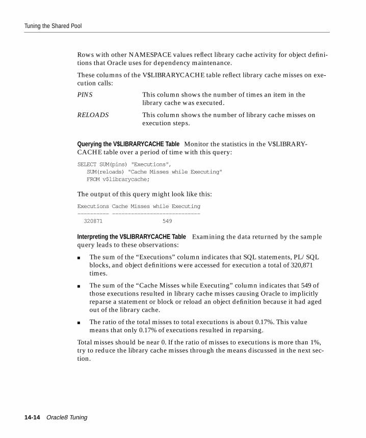
Tuning the Shared Pool
Rows with other NAMESPACE values reflect library cache activity for object defini-tions that Oracle uses for dependency maintenance.
These columns of the V$LIBRARYCACHE table reflect library cache misses on exe-cution calls:
Querying the V$LIBRARYCACHE Table Monitor the statistics in the V$LIBRARY-CACHE table over a period of time with this query:
SELECT SUM(pins) "Executions", SUM(reloads) "Cache Misses while Executing" FROM v$librarycache;
The output of this query might look like this:
Executions Cache Misses while Executing---------- ---------------------------- 320871 549
Interpreting the V$LIBRARYCACHE Table Examining the data returned by the samplequery leads to these observations:
■ The sum of the “Executions” column indicates that SQL statements, PL/SQLblocks, and object definitions were accessed for execution a total of 320,871times.
■ The sum of the “Cache Misses while Executing” column indicates that 549 ofthose executions resulted in library cache misses causing Oracle to implicitlyreparse a statement or block or reload an object definition because it had agedout of the library cache.
■ The ratio of the total misses to total executions is about 0.17%. This valuemeans that only 0.17% of executions resulted in reparsing.
Total misses should be near 0. If the ratio of misses to executions is more than 1%,try to reduce the library cache misses through the means discussed in the next sec-tion.
PINS This column shows the number of times an item in thelibrary cache was executed.
RELOADS This column shows the number of library cache misses onexecution steps.
14-14 Oracle8 Tuning
Tuning the Shared Pool
Reducing Library Cache MissesYou can reduce library cache misses by:
■ allocating additional memory for the library cache
■ writing identical SQL statements whenever possible
Allocating Additional Memory for the Library Cache You may be able to reduce librarycache misses on execution calls by allocating additional memory for the librarycache. To ensure that shared SQL areas remain in the cache once their SQL state-ments are parsed, increase the amount of memory available to the library cacheuntil the V$LIBRARYCACHE.RELOADS value is near 0. To increase the amount ofmemory available to the library cache, increase the value of the initialization param-eter SHARED_POOL_SIZE. The maximum value for this parameter depends onyour operating system. This measure will reduce implicit reparsing of SQL state-ments and PL/SQL blocks on execution.
To take advantage of additional memory available for shared SQL areas, you mayalso need to increase the number of cursors permitted for a session. You can do thisby increasing the value of the initialization parameter OPEN_CURSORS.
Be careful not to induce paging and swapping by allocating too much memory forthe library cache. The benefits of a library cache large enough to avoid cache missescan be partially offset by reading shared SQL areas into memory from disk when-ever you need to access them.
See Also: "SHARED_POOL_SIZE Too Small" on page 14-25
Writing Identical SQL Statements: Criteria You may be able to reduce library cachemisses on parse calls by ensuring that SQL statements and PL/SQL blocks use ashared SQL area whenever possible. Two separate occurrences of a SQL statementor PL/SQL block can use a shared SQL area if they are identical according to thesecriteria:
■ The text of the SQL statements or PL/SQL blocks must be identical, characterfor character, including spaces and case. For example, these statements cannotuse the same shared SQL area:
SELECT * FROM emp;SELECT * FROM emp;
These statements cannot use the same shared SQL area:
SELECT * FROM emp;SELECT * FROM Emp;
Tuning Memory Allocation 14-15
Tuning the Shared Pool
■ References to schema objects in the SQL statements or PL/SQL blocks mustresolve to the same object in the same schema.
For example, if the schemas of the users BOB and ED both contain an EMPtable and both users issue the following statement, their statements cannot usethe same shared SQL area:
SELECT * FROM emp;SELECT * FROM emp;
If both statements query the same table and qualify the table with the schema,as in the following statement, then they can use the same shared SQL area:
SELECT * FROM bob.emp;
■ Bind variables in the SQL statements must match in name and datatype. Forexample, these statements cannot use the same shared SQL area:
SELECT * FROM emp WHERE deptno = :department_no;SELECT * FROM emp WHERE deptno = :d_no;
■ The SQL statements must be optimized using the same optimization approachand, in the case of the cost-based approach, the same optimization goal. Forinformation on optimization approach and goal, see "Choosing a Goal for theCost-Based Approach" on page 8-6.
Writing Identical SQL Statements: Strategies Shared SQL areas are most useful forreducing library cache misses for multiple users running the same application. Dis-cuss these criteria with the developers of such applications and agree on strategiesto ensure that the SQL statements and PL/SQL blocks of an application can use thesame shared SQL areas:
■ Use bind variables rather than explicitly specified constants in your statementswhenever possible.
For example, the following two statements cannot use the same shared areabecause they do not match character for character:
SELECT ename, empno FROM emp WHERE deptno = 10;SELECT ename, empno FROM emp WHERE deptno = 20;
You can accomplish the goals of these statements by using the following state-ment that contains a bind variable, binding 10 for one occurrence of the state-ment and 20 for the other:
SELECT ename, empno FROM emp WHERE deptno = :department_no;
14-16 Oracle8 Tuning
Tuning the Shared Pool
The two occurrences of the statement can then use the same shared SQL area.
■ Be sure that users of the application do not change the optimization approachand goal for their individual sessions.
■ You can also increase the likelihood that SQL statements issued by differentapplications can share SQL areas by establishing these policies among thedevelopers of the applications:
■ Standardize naming conventions for bind variables and spacing conven-tions for SQL statements and PL/SQL blocks.
■ Use stored procedures whenever possible. Multiple users issuing the samestored procedure automatically use the same shared PL/SQL area. Sincestored procedures are stored in a parsed form, they eliminate run-time pars-ing altogether.
Using CURSOR_SPACE_FOR_TIME to Speed Access to Shared SQL Areas:If you have no library cache misses, you may still be able to speed execution callsby setting the value of the initialization parameter CURSOR_SPACE_FOR_TIME.This parameter specifies whether a shared SQL area can be deallocated from thelibrary cache to make room for a new SQL statement.
■ If the value of this parameter is FALSE (the default), a shared SQL area can bedeallocated from the library cache regardless of whether application cursorsassociated with its SQL statement are open. In this case, Oracle must verify thata shared SQL area containing the SQL statement is in the library cache.
■ If the value of this parameter is TRUE, a shared SQL area can be deallocatedonly when all application cursors associated with its statement are closed. Inthis case, Oracle need not verify that a shared SQL area is in the cache, becausethe shared SQL area can never be deallocated while an application cursor asso-ciated with it is open.
Setting the value of the parameter to TRUE saves Oracle a small amount of timeand may slightly improve the performance of execution calls. This value also pre-vents the deallocation of private SQL areas until associated application cursors areclosed.
Do not set the value of CURSOR_SPACE_FOR_TIME to TRUE if you have foundlibrary cache misses on execution calls. Such library cache misses indicate that theshared pool is not large enough to hold the shared SQL areas of all concurrentlyopen cursors. If the value is TRUE and the shared pool has no space for a new SQLstatement, the statement cannot be parsed and Oracle returns an error saying thatthere is no more shared memory. If the value is FALSE and there is no space for a
Tuning Memory Allocation 14-17
Tuning the Shared Pool
new statement, Oracle deallocates an existing shared SQL area. Although deallocat-ing a shared SQL area results in a library cache miss later, it is preferable to an errorhalting your application because a SQL statement cannot be parsed.
Do not set the value of CURSOR_SPACE_FOR_TIME to TRUE if the amount ofmemory available to each user for private SQL areas is scarce. This value also pre-vents the deallocation of private SQL areas associated with open cursors. If the pri-vate SQL areas for all concurrently open cursors fills the user’s available memoryso that there is no space to allocate a private SQL area for a new SQL statement, thestatement cannot be parsed and Oracle returns an error indicating that there is notenough memory.
Caching Session CursorsIf an application repeatedly issues parse calls on the same set of SQL statements,the reopening of the session cursors can affect system performance. Session cursorscan be stored in a session cursor cache. This feature can be particularly useful forapplications designed using Oracle Forms, because switching from one form toanother closes all session cursors associated with the first form.
Oracle uses the shared SQL area to determine whether more than three parserequests have been issued on a given statement. If so, Oracle assumes the sessioncursor associated with the statement should be cached and moves the cursor intothe session cursor cache. Subsequent requests to parse that SQL statement by thesame session will then find the cursor in the session cursor cache.
To enable caching of session cursors, you must set the initialization parameterSESSION_CACHED_CURSORS. The value of this parameter is a positive integerspecifying the maximum number of session cursors kept in the cache. A leastrecently used (LRU) algorithm ages out entries in the session cursor cache to makeroom for new entries when needed.
You can also enable the session cursor cache dynamically with the statementALTER SESSION SET SESSION_CACHED_CURSORS.
To determine whether the session cursor cache is sufficiently large for yourinstance, you can examine the session statistic “session cursor cache hits” in theV$SESSTAT view. This statistic counts the number of times a parse call found a cur-sor in the session cursor cache. If this statistic is a relatively low percentage of thetotal parse call count for the session, you should consider settingSESSION_CACHED_CURSORS to a larger value.
14-18 Oracle8 Tuning
Tuning the Shared Pool
Tuning the Data Dictionary CacheThis section describes how to monitor data dictionary cache activity and reducemisses.
Monitoring Data Dictionary Cache ActivityDetermine whether misses on the data dictionary cache are affecting the perfor-mance of Oracle. You can examine cache activity by querying the V$ROWCACHEtable as described in the following sections.
Misses on the data dictionary cache are to be expected in some cases. Uponinstance startup, the data dictionary cache contains no data, so any SQL statementissued is likely to result in cache misses. As more data is read into the cache, thelikelihood of cache misses should decrease. Eventually the database should reach a“steady state” in which the most frequently used dictionary data is in the cache. Atthis point, very few cache misses should occur. To tune the cache, examine its activ-ity only after your application has been running.
The V$ROWCACHE View Statistics reflecting data dictionary activity are kept in thedynamic performance table V$ROWCACHE. By default, this table is available onlyto the user SYS and to users granted SELECT ANY TABLE system privilege, suchas SYSTEM.
Each row in this table contains statistics for a single type of the data dictionaryitem. These statistics reflect all data dictionary activity since the most recentinstance startup. These columns in the V$ROWCACHE table reflect the use andeffectiveness of the data dictionary cache:
PARAMETER Identifies a particular data dictionary item. For each row, thevalue in this column is the item prefixed by dc_. For exam-ple, in the row that contains statistics for file descriptions,this column has the value dc_files.
GETS Shows the total number of requests for information on thecorresponding item. For example, in the row that containsstatistics for file descriptions, this column has the total num-ber of requests for file descriptions data.
GETMISSES Shows the number of data requests resulting in cache misses.
Tuning Memory Allocation 14-19
Tuning the Shared Pool
Querying the V$ROWCACHE Table Use the following query to monitor the statistics inthe V$ROWCACHE table over a period of time while your application is running:
SELECT SUM(gets) "Data Dictionary Gets", SUM(getmisses) "Data Dictionary Cache Get Misses" FROM v$rowcache;
The output of this query might look like this:
Data Dictionary Gets Data Dictionary Cache Get Misses-------------------- -------------------------------- 1439044 3120
Interpreting the V$ROWCACHE Table Examining the data returned by the samplequery leads to these observations:
■ The sum of the GETS column indicates that there were a total of 1,439,044requests for dictionary data.
■ The sum of the GETMISSES column indicates that 3120 of the requests for dic-tionary data resulted in cache misses.
■ The ratio of the sums of GETMISSES to GETS is about 0.2%.
Reducing Data Dictionary Cache MissesExamine cache activity by monitoring the sums of the GETS and GETMISSES col-umns. For frequently accessed dictionary caches, the ratio of total GETMISSES tototal GETS should be less than 10% or 15%. If the ratio continues to increase abovethis threshold while your application is running, you should consider increasingthe amount of memory available to the data dictionary cache. To increase the mem-ory available to the cache, increase the value of the initialization parameterSHARED_POOL_SIZE. The maximum value for this parameter depends on youroperating system.
Tuning the Shared Pool with the Multithreaded ServerIn the multithreaded server architecture, Oracle stores session information in theshared pool rather than in the memory of user processes. Session informationincludes private SQL areas. If you are using the multithreaded server architecture,you may need to make your shared pool larger to accommodate session informa-tion. You can increase the size of the shared pool by increasing the value of theSHARED_POOL_SIZE initialization parameter. This section discusses measuringthe size of session information by querying the dynamic performance tableV$SESSTAT.
14-20 Oracle8 Tuning
Tuning the Shared Pool
With very high numbers of connected users, the only way to reduce memory usageto an acceptable level may be to go to three-tier connections. This by-product ofusing a TP monitor is feasible only with a pure transactional model, because nolocks or uncommitted DML can be held between calls. Oracle’s multithreadedserver (MTS) is much less restrictive of the application design than a TP monitor. Itdramatically reduces operating system process count, because it normally requiresonly 5 threads per CPU. It still requires a minimum of about 300K bytes of contextper connected user.
The V$SESSTAT TableOracle collects statistics on total memory used by a session and stores them in thedynamic performance table V$SESSTAT. By default, this table is available only tothe user SYS and to users granted SELECT ANY TABLE system privilege, such asSYSTEM. These statistics are useful for measuring session memory use:
To find the value, query V$STATNAME as described in "Technique 3" on page 14-8.
Querying the V$SESSTAT TableYou can use this query to decide how much larger to make the shared pool if youare using a multithreaded server. Issue these queries while your application is run-ning:
SELECT SUM(value) || ’ bytes’ "Total memory for all sessions" FROM v$sesstat, v$statname WHERE name = ’session uga memory’ AND v$sesstat.statistic# = v$statname.statistic#;SELECT SUM(value) || ’ bytes’ "Total max mem for all sessions" FROM v$sesstat, v$statname WHERE name = ’session uga memory max’ AND v$sesstat.statistic# = v$statname.statistic#;
These queries also select from the dynamic performance table V$STATNAME toobtain internal identifiers for session memory and max session memory. The results ofthese queries might look like this:
session uga memory The value of this statistic is the amount of memory inbytes allocated to the session.
session uga memorymax
The value of this statistic is the maximum amount ofmemory in bytes ever allocated to the session.
Tuning Memory Allocation 14-21
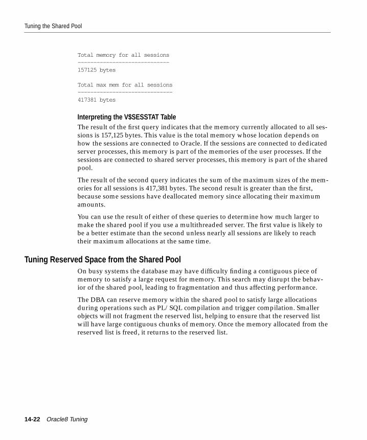
Tuning the Shared Pool
Total memory for all sessions-----------------------------157125 bytes
Total max mem for all sessions------------------------------417381 bytes
Interpreting the V$SESSTAT TableThe result of the first query indicates that the memory currently allocated to all ses-sions is 157,125 bytes. This value is the total memory whose location depends onhow the sessions are connected to Oracle. If the sessions are connected to dedicatedserver processes, this memory is part of the memories of the user processes. If thesessions are connected to shared server processes, this memory is part of the sharedpool.
The result of the second query indicates the sum of the maximum sizes of the mem-ories for all sessions is 417,381 bytes. The second result is greater than the first,because some sessions have deallocated memory since allocating their maximumamounts.
You can use the result of either of these queries to determine how much larger tomake the shared pool if you use a multithreaded server. The first value is likely tobe a better estimate than the second unless nearly all sessions are likely to reachtheir maximum allocations at the same time.
Tuning Reserved Space from the Shared PoolOn busy systems the database may have difficulty finding a contiguous piece ofmemory to satisfy a large request for memory. This search may disrupt the behav-ior of the shared pool, leading to fragmentation and thus affecting performance.
The DBA can reserve memory within the shared pool to satisfy large allocationsduring operations such as PL/SQL compilation and trigger compilation. Smallerobjects will not fragment the reserved list, helping to ensure that the reserved listwill have large contiguous chunks of memory. Once the memory allocated from thereserved list is freed, it returns to the reserved list.
14-22 Oracle8 Tuning
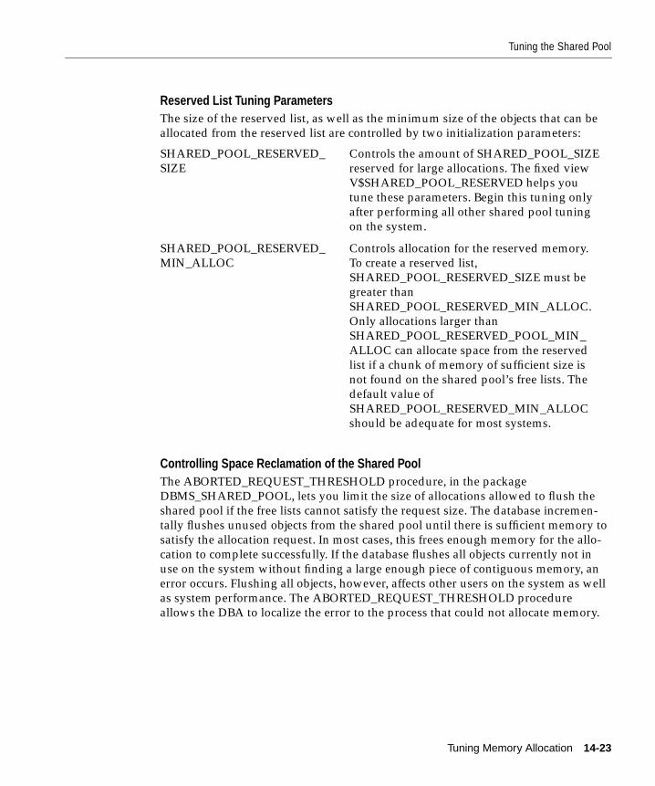
Tuning the Shared Pool
Reserved List Tuning ParametersThe size of the reserved list, as well as the minimum size of the objects that can beallocated from the reserved list are controlled by two initialization parameters:
Controlling Space Reclamation of the Shared PoolThe ABORTED_REQUEST_THRESHOLD procedure, in the packageDBMS_SHARED_POOL, lets you limit the size of allocations allowed to flush theshared pool if the free lists cannot satisfy the request size. The database incremen-tally flushes unused objects from the shared pool until there is sufficient memory tosatisfy the allocation request. In most cases, this frees enough memory for the allo-cation to complete successfully. If the database flushes all objects currently not inuse on the system without finding a large enough piece of contiguous memory, anerror occurs. Flushing all objects, however, affects other users on the system as wellas system performance. The ABORTED_REQUEST_THRESHOLD procedureallows the DBA to localize the error to the process that could not allocate memory.
SHARED_POOL_RESERVED_SIZE
Controls the amount of SHARED_POOL_SIZEreserved for large allocations. The fixed viewV$SHARED_POOL_RESERVED helps youtune these parameters. Begin this tuning onlyafter performing all other shared pool tuningon the system.
SHARED_POOL_RESERVED_MIN_ALLOC
Controls allocation for the reserved memory.To create a reserved list,SHARED_POOL_RESERVED_SIZE must begreater thanSHARED_POOL_RESERVED_MIN_ALLOC.Only allocations larger thanSHARED_POOL_RESERVED_POOL_MIN_ALLOC can allocate space from the reservedlist if a chunk of memory of sufficient size isnot found on the shared pool’s free lists. Thedefault value ofSHARED_POOL_RESERVED_MIN_ALLOCshould be adequate for most systems.
Tuning Memory Allocation 14-23
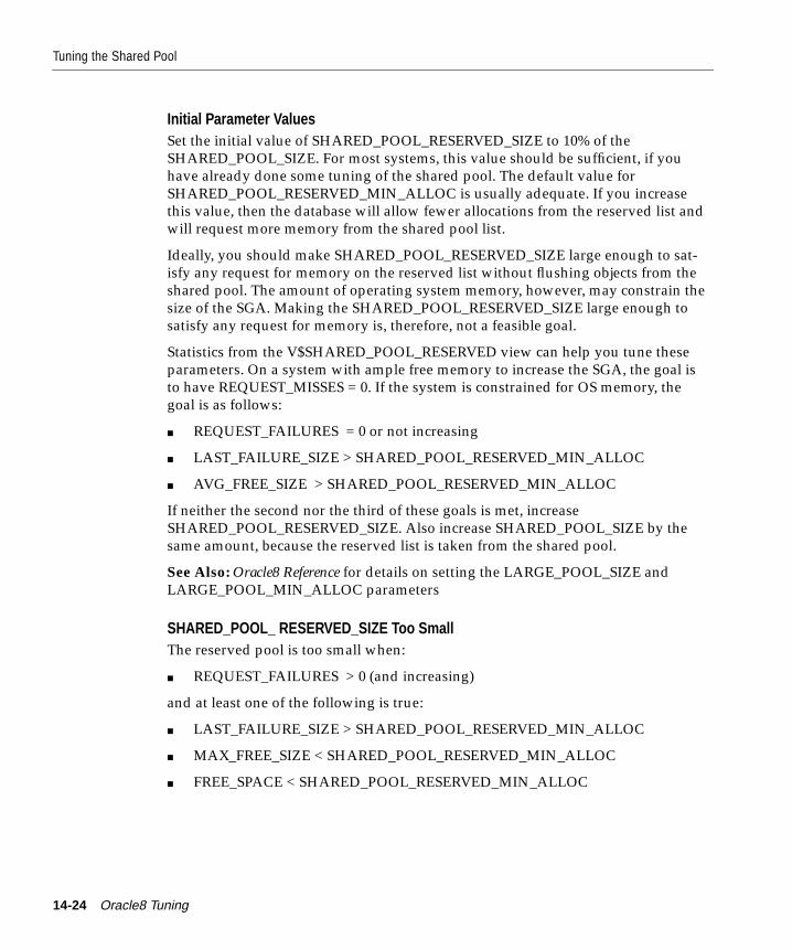
Tuning the Shared Pool
Initial Parameter ValuesSet the initial value of SHARED_POOL_RESERVED_SIZE to 10% of theSHARED_POOL_SIZE. For most systems, this value should be sufficient, if youhave already done some tuning of the shared pool. The default value forSHARED_POOL_RESERVED_MIN_ALLOC is usually adequate. If you increasethis value, then the database will allow fewer allocations from the reserved list andwill request more memory from the shared pool list.
Ideally, you should make SHARED_POOL_RESERVED_SIZE large enough to sat-isfy any request for memory on the reserved list without flushing objects from theshared pool. The amount of operating system memory, however, may constrain thesize of the SGA. Making the SHARED_POOL_RESERVED_SIZE large enough tosatisfy any request for memory is, therefore, not a feasible goal.
Statistics from the V$SHARED_POOL_RESERVED view can help you tune theseparameters. On a system with ample free memory to increase the SGA, the goal isto have REQUEST_MISSES = 0. If the system is constrained for OS memory, thegoal is as follows:
■ REQUEST_FAILURES = 0 or not increasing
■ LAST_FAILURE_SIZE > SHARED_POOL_RESERVED_MIN_ALLOC
■ AVG_FREE_SIZE > SHARED_POOL_RESERVED_MIN_ALLOC
If neither the second nor the third of these goals is met, increaseSHARED_POOL_RESERVED_SIZE. Also increase SHARED_POOL_SIZE by thesame amount, because the reserved list is taken from the shared pool.
See Also: Oracle8 Reference for details on setting the LARGE_POOL_SIZE andLARGE_POOL_MIN_ALLOC parameters
SHARED_POOL_ RESERVED_SIZE Too SmallThe reserved pool is too small when:
■ REQUEST_FAILURES > 0 (and increasing)
and at least one of the following is true:
■ LAST_FAILURE_SIZE > SHARED_POOL_RESERVED_MIN_ALLOC
■ MAX_FREE_SIZE < SHARED_POOL_RESERVED_MIN_ALLOC
■ FREE_SPACE < SHARED_POOL_RESERVED_MIN_ALLOC
14-24 Oracle8 Tuning

Tuning the Shared Pool
You have two options, depending on SGA size constraints:
■ Increase SHARED_POOL_RESERVED_SIZE and SHARED_POOL_SIZEaccordingly.
■ Increase SHARED_POOL_RESERVED_MIN_ALLOC (but you may need toincrease SHARED_POOL_SIZE).
The first option increases the amount of memory available on the reserved list with-out having an impact on users not allocating memory from the reserved list. Thesecond options reduces the number of allocations allowed to use memory from thereserved list; doing so, however, increases the normal shared pool, which may havean impact on other users on the system.
SHARED_POOL_ RESERVED_SIZE Too LargeToo much memory may have been allocated to the reserved list if:
■ REQUEST_MISS = 0 or not increasing
■ FREE_MEMORY = > 50% of SHARED_POOL_RESERVED_SIZE minimum
You have two options:
■ Decrease SHARED_POOL_RESERVED_SIZE.
■ Decrease SHARED_POOL_RESERVED_MIN_ALLOC (if not the default value).
SHARED_POOL_SIZE Too SmallThe V$SHARED_POOL_RESERVED fixed table can also indicate whenSHARED_POOL_SIZE is too small. This may be the case if:
■ REQUEST_FAILURES > 0 and increasing
■ LAST_FAILURE_SIZE < SHARED_POOL_RESERVED_MIN_ALLOC
Then you have two options, if you have enabled the reserved list:
■ Decrease SHARED_POOL_RESERVED_SIZE.
■ Decrease SHARED_POOL_RESERVED_MIN_ALLOC (if set larger than thedefault).
If you have not enabled the reserved list, you could:
■ Increase SHARED_POOL_SIZE.
Tuning Memory Allocation 14-25
Tuning the Buffer Cache
Tuning the Buffer CacheYou can use or bypass the Oracle buffer cache for particular operations. Note thatOracle bypasses the buffer cache for sorting and parallel reads. For operations thatdo use the buffer cache, this section explains:
■ Evaluating Buffer Cache Activity by Means of the Cache Hit Ratio
■ Raising Cache Hit Ratio by Reducing Buffer Cache Misses
■ Removing Unnecessary Buffers when Cache Hit Ratio Is High
After tuning private SQL and PL/SQL areas and the shared pool, you can devotethe remaining available memory to the buffer cache. It may be necessary to repeatthe steps of memory allocation after the initial pass through the process. Subse-quent passes allow you to make adjustments in earlier steps based on changes inlater steps. For example, if you increase the size of the buffer cache, you may needto allocate more memory to Oracle to avoid paging and swapping.
Evaluating Buffer Cache Activity by Means of the Cache Hit RatioPhysical I/O takes significant time (typically in excess of 15 msec) and alsoincreases the CPU resource required, owing to the path length in device driversand operating system event schedulers. Your goal is to reduce this overhead as faras possible by making it more likely that the required block will be in memory. Theextent to which you achieve this is measured using the cache hit ratio. Within Ora-cle this term applies specifically to the database buffer cache.
Calculating the Cache Hit RatioOracle collects statistics that reflect data access and stores them in the dynamic per-formance table V$SYSSTAT. By default, this table is available only to the user SYSand to users (such as SYSTEM) who have been granted SELECT ANY TABLE sys-tem privilege. Information in the V$SYSSTAT table can also be obtained throughthe Simple Network Management Protocol (SNMP).
These statistics are useful for tuning the buffer cache:
db block gets,consistent gets
The sum of the values of these statistics is the total number ofrequests for data. This value includes requests satisfied byaccess to buffers in memory.
physical reads The value of this statistic is the total number of requests fordata resulting in access to datafiles on disk.
14-26 Oracle8 Tuning
Tuning the Buffer Cache
Monitor these statistics as follows over a period of time while your application isrunning:
SELECT name, value FROM v$sysstat WHERE name IN (’db block gets’, ’consistent gets’, ’physical reads’);
The output of this query might look like this:
NAME VALUE------------------------------------------------------ ----------db block gets 85792consistent gets 278888physical reads 23182
Calculate the hit ratio for the buffer cache with this formula:
Hit Ratio = 1 - ( physical reads / (db block gets + consistent gets) )
Based on the statistics obtained by the example query, the buffer cache hit ratio is94%.
Evaluating the Cache Hit RatioWhen looking at the cache hit ratio, bear in mind that blocks encountered during a“long” full table scan are not put at the head of the LRU list; therefore repeatedscanning will not cause the blocks to be cached.
Repeated scanning of the same large table is rarely the most efficient approach. Itmay be better to perform all of the processing in a single pass, even if this meansthat the overnight batch suite can no longer be implemented as a SQL*Plus scriptwhich contains no PL/SQL. The solution therefore lies at the design or implementa-tion level.
Note: The CACHE_SIZE_THRESHOLD parameter sets the maximum size of atable to be cached, in blocks; it is equal to one tenth of DB_BLOCK_BUFFERS. On aper-table basis, this parameter enables you to determine which tables should andshould not be cached.
Production sites running with thousands or tens of thousands of buffers rarely usememory effectively. In any large database running an OLTP application, in anygiven unit of time, most rows will be accessed either one or zero times. On thisbasis there is little point in keeping the row (or the block that contains it) in mem-ory for very long following its use.
Tuning Memory Allocation 14-27
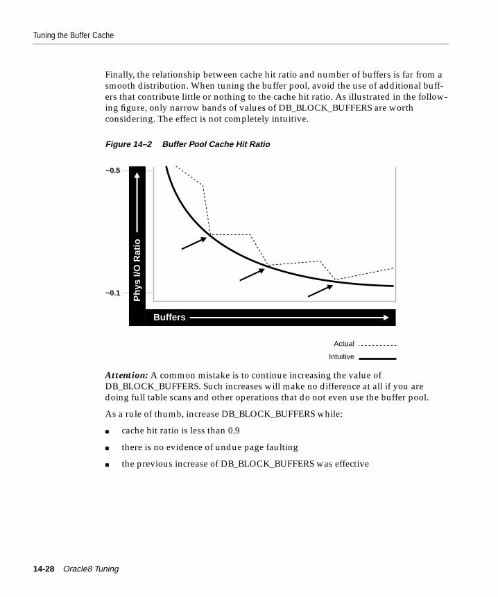
Tuning the Buffer Cache
Finally, the relationship between cache hit ratio and number of buffers is far from asmooth distribution. When tuning the buffer pool, avoid the use of additional buff-ers that contribute little or nothing to the cache hit ratio. As illustrated in the follow-ing figure, only narrow bands of values of DB_BLOCK_BUFFERS are worthconsidering. The effect is not completely intuitive.
Figure 14–2 Buffer Pool Cache Hit Ratio
Attention: A common mistake is to continue increasing the value ofDB_BLOCK_BUFFERS. Such increases will make no difference at all if you aredoing full table scans and other operations that do not even use the buffer pool.
As a rule of thumb, increase DB_BLOCK_BUFFERS while:
■ cache hit ratio is less than 0.9
■ there is no evidence of undue page faulting
■ the previous increase of DB_BLOCK_BUFFERS was effective
Buffers
Ph
ys I/
O R
atio
~0.5
~0.1
Actual
Intuitive
14-28 Oracle8 Tuning
Tuning the Buffer Cache
Determining Which Buffers Are in the PoolThe CATPARR.SQL script creates the view V$BH, which shows the file numberand block number of blocks that currently reside within the SGA. Although CAT-PARR.SQL is primarily intended for use in parallel server environments, you canrun it as SYS even if the instance is always started in exclusive mode.
Perform a query like the following:
SELECT file#, COUNT(block#), COUNT (DISTINCT file# || block#)FROM V$BHGROUP BY file#
Raising Cache Hit Ratio by Reducing Buffer Cache MissesIf your hit ratio is low, perhaps less than 60% or 70%, then you may want toincrease the number of buffers in the cache to improve performance. To make thebuffer cache larger, increase the value of the initialization parameterDB_BLOCK_BUFFERS.
Oracle can collect statistics that estimate the performance gain that would resultfrom increasing the size of your buffer cache. With these statistics, you can estimatehow many buffers to add to your cache.
The V$RECENT_BUCKET ViewThe virtual table V$RECENT_BUCKET contains statistics that estimate the perfor-mance of a larger cache. Each row in the table reflects the relative performancevalue of adding a buffer to the cache. This table can only be accessed only by theuser SYS. The following are the columns of the V$RECENT_BUCKET view
For example, in the first row of the table, the ROWNUM value is 0 and the COUNTvalue is the number of cache hits to be gained by adding the first additional bufferto the cache. In the second row, the ROWNUM value is 1 and the COUNT value isthe number of cache hits for the second additional buffer.
Note: The GV$CURRENT_BUCKET and GV$RECENT_BUCKET views providethe instance identifier (INST_ID) along with the count. If necessary, you can infer
ROWNUM The value of this column is one less than the number of buffers thatwould potentially be added to the cache.
COUNT The value of this column is the number of additional cache hits thatwould be obtained by adding buffer number ROWNUM+1 to thecache.
Tuning Memory Allocation 14-29
Tuning the Buffer Cache
the INDX value: the nth entry for a particular instance would reflect index n forthat instance.
Enabling the V$RECENT_BUCKET ViewThe collection of statistics in the V$RECENT_BUCKET view is controlled by the ini-tialization parameter DB_BLOCK_LRU_EXTENDED_STATISTICS. The value ofthis parameter determines the number of rows in the V$RECENT_BUCKET view.The default value of this parameter is 0, which means the default behavior is not tocollect statistics.
To enable the collection of statistics in the V$RECENT_BUCKET view, set the valueof DB_BLOCK_LRU_EXTENDED_STATISTICS. For example, if you set the value ofthe parameter to 100, Oracle will collect 100 rows of statistics, each row reflectingthe addition of one buffer, up to 100 extra buffers.
Collecting these statistics incurs some performance overhead, which is propor-tional to the number of rows in the table. To avoid this overhead, collect statisticsonly when you are tuning the buffer cache; disable the collection of statistics whenyou are finished tuning.
Querying the V$RECENT_BUCKET ViewFrom the information in the V$RECENT_BUCKET view, you can predict the poten-tial gains of increasing the cache size. For example, to determine how many morecache hits would occur if you added 20 buffers to the cache, query theV$RECENT_BUCKET view with the following SQL statement:
SELECT SUM(count) ach FROM V$RECENT_BUCKET WHERE ROWNUM < 20;
You can also determine how these additional cache hits would affect the hit ratio.Use the following formula to calculate the hit ratio based on the values of the statis-tics db block gets, consistent gets, and physical reads and the number of additionalcache hits (ACH) returned by the query:
Hit Ratio = 1 - (physical reads - ACH / (db block gets + consistent gets) )
14-30 Oracle8 Tuning
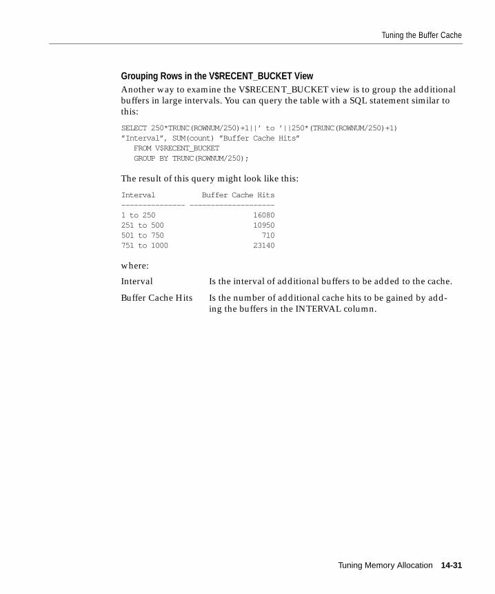
Tuning the Buffer Cache
Grouping Rows in the V$RECENT_BUCKET ViewAnother way to examine the V$RECENT_BUCKET view is to group the additionalbuffers in large intervals. You can query the table with a SQL statement similar tothis:
SELECT 250*TRUNC(ROWNUM/250)+1||’ to ’||250*(TRUNC(ROWNUM/250)+1)”Interval”, SUM(count) ”Buffer Cache Hits” FROM V$RECENT_BUCKET GROUP BY TRUNC(ROWNUM/250);
The result of this query might look like this:
Interval Buffer Cache Hits--------------- --------------------1 to 250 16080251 to 500 10950501 to 750 710751 to 1000 23140
where:
Interval Is the interval of additional buffers to be added to the cache.
Buffer Cache Hits Is the number of additional cache hits to be gained by add-ing the buffers in the INTERVAL column.
Tuning Memory Allocation 14-31
Tuning the Buffer Cache
Examining the query output leads to these observations:
■ If 250 buffers were added to the cache, 16,080 cache hits would be gained.
■ If 250 more buffers were added for a total of 500 additional buffers, 10,950cache hits would be gained in addition to the 16,080 cache hits from the first250 buffers. This means that adding 500 buffers would yield a total of 27,030additional cache hits.
■ If 250 more buffers were added for a total of 750 additional buffers, 710 cachehits would be gained, yielding a total of 27,740 additional cache hits.
■ If 250 buffers were added to the cache for a total of 1000 additional buffers,23,140 cache hits would be gained, yielding a total of 50,880 additional cachehits.
Based on these observations, decide how many buffers to add to the cache. In thiscase, you may make these decisions:
■ It is wise to add 250 or 500 buffers, provided memory resources are available.Both of these increments offer significant performance gains.
■ It is unwise to add 750 buffers. Nearly the entire performance gain made bysuch an increase can be made by adding 500 buffers instead. Also, the memoryallocated to the additional 250 buffers may be better used by some other Oraclememory structure.
■ It is wise to add 1000 buffers, provided memory resources are available. Theperformance gain from adding 1000 buffers to the cache is significantly greaterthan the gains from adding 250, 500, or 750 buffers.
Removing Unnecessary Buffers when Cache Hit Ratio Is HighIf your hit ratio is high, your cache is probably large enough to hold your most fre-quently accessed data. In this case, you may be able to reduce the cache size andstill maintain good performance. To make the buffer cache smaller, reduce thevalue of the initialization parameter DB_BLOCK_BUFFERS. The minimum valuefor this parameter is 4. You can apply any leftover memory to other Oracle memorystructures.
Oracle can collect statistics to predict buffer cache performance based on a smallercache size. Examining these statistics can help you determine how small you canafford to make your buffer cache without adversely affecting performance.
14-32 Oracle8 Tuning
Tuning the Buffer Cache
The V$CURRENT_BUCKET ViewThe V$CURRENT_BUCKET view contains the statistics that estimate the perfor-mance of a smaller cache. The V$CURRENT_BUCKET view is similar in structureto the V$RECENT_BUCKET view. This table can be accessed only by the user SYS.The following are the columns of the V$CURRENT_BUCKET view:
The number of rows in this table is equal to the number of buffers in your buffercache. Each row in the table reflects the number of cache hits attributed to a singlebuffer. For example, in the second row, the ROWNUM value is 1 and the COUNTvalue is the number of cache hits for the second buffer. In the third row, theROWNUM value is 2 and the COUNT value is the number of cache hits for thethird buffer.
The first row of the table contains special information. The ROWNUM value is 0and the COUNT value is the total number of blocks moved into the first buffer inthe cache.
Enabling the V$CURRENT_BUCKET ViewThe collection of statistics in the V$CURRENT_BUCKET view is controlled by theinitialization parameter DB_BLOCK_LRU_STATISTICS. The value of this parame-ter determines whether Oracle collects the statistics. The default value for thisparameter is FALSE, which means that the default behavior is not to collect statis-tics.
To enable the collection of statistics in the V$CURRENT_BUCKET view, set thevalue of DB_BLOCK_LRU_STATISTICS to TRUE.
Collecting these statistics incurs some performance overhead. To minimize thisoverhead, collect statistics only when you are tuning the buffer cache; disable thecollection of statistics when you are finished tuning.
ROWNUM The potential number of buffers in the cache.
COUNT The number of cache hits attributable to buffer number ROWNUM.
Tuning Memory Allocation 14-33
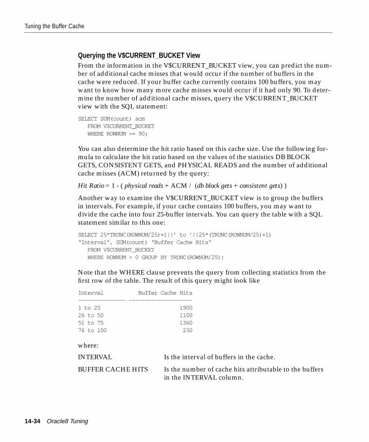
Tuning the Buffer Cache
Querying the V$CURRENT_BUCKET ViewFrom the information in the V$CURRENT_BUCKET view, you can predict the num-ber of additional cache misses that would occur if the number of buffers in thecache were reduced. If your buffer cache currently contains 100 buffers, you maywant to know how many more cache misses would occur if it had only 90. To deter-mine the number of additional cache misses, query the V$CURRENT_BUCKETview with the SQL statement:
SELECT SUM(count) acm FROM V$CURRENT_BUCKET WHERE ROWNUM >= 90;
You can also determine the hit ratio based on this cache size. Use the following for-mula to calculate the hit ratio based on the values of the statistics DB BLOCKGETS, CONSISTENT GETS, and PHYSICAL READS and the number of additionalcache misses (ACM) returned by the query:
Hit Ratio = 1 - ( physical reads + ACM / (db block gets + consistent gets) )
Another way to examine the V$CURRENT_BUCKET view is to group the buffersin intervals. For example, if your cache contains 100 buffers, you may want todivide the cache into four 25-buffer intervals. You can query the table with a SQLstatement similar to this one:
SELECT 25*TRUNC(ROWNUM/25)+1||’ to ’||25*(TRUNC(ROWNUM/25)+1)"Interval", SUM(count) "Buffer Cache Hits" FROM V$CURRENT_BUCKET WHERE ROWNUM > 0 GROUP BY TRUNC(ROWNUM/25);
Note that the WHERE clause prevents the query from collecting statistics from thefirst row of the table. The result of this query might look like
Interval Buffer Cache Hits--------------- --------------------1 to 25 190026 to 50 110051 to 75 136076 to 100 230
where:
INTERVAL Is the interval of buffers in the cache.
BUFFER CACHE HITS Is the number of cache hits attributable to the buffersin the INTERVAL column.
14-34 Oracle8 Tuning
Tuning the Buffer Cache
Examining the query output leads to these observations:
■ The last 25 buffers in the cache (buffers 76 to 100) contribute 230 cache hits. Ifthe cache were reduced in size by 25 buffers, 230 cache hits would be lost.
■ The third 25-buffer interval (buffers 51 to 75) contributes 1,360 cache hits. Ifthese buffers were removed from the cache, 1,360 cache hits would be lost inaddition to the 230 cache hits lost for buffers 76 to 100. Removing 50 bufferswould result in losing a total of 1,590 cache hits.
■ The second 25-buffer interval (buffers 26 to 50) contributes 1,100 cache hits.Removing 75 buffers from the cache would result in losing a total of 2,690cache hits.
■ The first 25 buffers in the cache (buffers 1 to 25) contribute 1,900 cache hits.
Based on these observations, decide whether to reduce the size of the cache. In thiscase, you may make these decisions:
■ If memory is scarce, it may be wise to remove 25 buffers from the cache. Thebuffers 76 to 100 contribute relatively few cache hits compared to the totalcache hits contributed by the entire cache. Removing 25 buffers will not signifi-cantly reduce cache performance, and the leftover memory may be better usedby other Oracle memory structures.
■ It is unwise to remove more than 25 buffers from the cache. For example,removing 50 buffers would reduce cache performance significantly. The cachehits contributed by these buffers is a significant portion of the total.
Tuning Memory Allocation 14-35
Tuning Multiple Buffer Pools
Tuning Multiple Buffer PoolsThis section covers:
■ Overview of the Multiple Buffer Pool Feature
■ When to Use Multiple Buffer Pools
■ Tuning the Buffer Cache Using Multiple Buffer Pools
■ Enabling Multiple Buffer Pools
■ Using Multiple Buffer Pools
■ Dictionary Views Showing Default Buffer Pools
■ How to Size Each Buffer Pool
■ How to Recognize and Eliminate LRU Latch Contention
14-36 Oracle8 Tuning
Tuning Multiple Buffer Pools
Overview of the Multiple Buffer Pool FeatureSchema objects are referenced with varying usage patterns; therefore, their cachebehavior may be quite different. Multiple buffer pools enable you to address thesedifferences. You can use a “keep” buffer pool to maintain an object in the buffercache, and a “recycle” buffer pool to prevent an object from taking up unnecessaryspace in the cache. When an object is allocated to a cache, all blocks from that objectare placed in that cache. Oracle maintains a default cache for objects that have notbeen assigned to one of the buffer pools.
Each buffer pool in Oracle8 comprises a number of working sets. A different num-ber of sets can be allocated for each buffer pool. All sets use the same LRU replace-ment policy. A strict LRU aging policy provides very good hit rates in most cases,but you can sometimes improve the hit rate by providing some hints.
The main problem with the LRU list occurs when a very large segment is accessedfrequently in a random fashion. Here, “very large” means large compared to thesize of the cache. Any single segment that accounts for a substantial portion (morethan 10%) of nonsequential physical reads is probably one of these segments. Ran-dom reads to such a large segment can cause buffers that contain data for other seg-ments to be aged out of the cache. The large segment ends up consuming a largepercentage of the cache, but does not benefit from the cache.
Very frequently accessed segments are not affected by large segment reads, becausetheir buffers are warmed frequently enough that they do not age out of the cache.The main trouble occurs with “warm” segments that are not accessed frequentlyenough to survive the buffer flushing caused by the large segment reads.
You have two options for solving this problem. One is to move the large segmentinto a separate “recycle” cache so that it does not disturb the other segments. Therecycle cache should be smaller than the default cache and should reuse buffersmore quickly than the default cache.
The other approach is to move the small warm segments into a separate “keep”cache that is not used at all for large segments. The keep cache can be sized to mini-mize misses in the cache. You can make the response times for specific queriesmore predictable by putting the segments accessed by the queries in the keep cacheto ensure that they are never aged out.
Tuning Memory Allocation 14-37
Tuning Multiple Buffer Pools
When to Use Multiple Buffer PoolsWhen you examine system I/O performance, you should analyze the schema anddetermine whether or not multiple buffer pools would be advantageous. Considera keep cache if there are small, frequently accessed tables that require quickresponse time. Very large tables with random I/O are good candidates for a recyclecache.
Use the following steps to determine the percentage of the cache used by an indi-vidual object at a given point in time:
1. Find the Oracle internal object number of the segment by entering:
SELECT data_object_id, object_type FROM user_objectsWHERE object_name = '<segment_name>';
Since two objects can have the same name (if they are different types of object),you can use the OBJECT_TYPE column to identify the object of interest. If theobject is owned by another user, then use the view DBA_OBJECTS orALL_OBJECTS instead of USER_OBJECTS.
2. Find the number of buffers in the buffer cache for segment_name:
SELECT count(*) buffers FROM x$bh WHERE obj = <data_object_id>;
where data_object_id is from Step 1.
3. Find the total number of buffers in the instance:
SELECT value "total buffers" FROM v$parameterWHERE name = 'db_block_buffers';
4. Calculate the ratio of buffers to total buffers, to obtain the percentage of thecache currently used by segment_name.
Note: This technique works only for a single segment; for a partitioned object,the query must be run for each partition.
If the number of local block gets equals the number of physical reads for statementsinvolving such objects, consider employing a recycle cache because of the limitedusefulness of the buffer cache for the objects.
% cache used by segment_name =buffers (Step 2)
total buffers (Step 3)
14-38 Oracle8 Tuning
Tuning Multiple Buffer Pools
Tuning the Buffer Cache Using Multiple Buffer PoolsWhen you partition your buffer cache into multiple buffer pools, each buffer poolcan be used for blocks from objects that are accessed in different ways. If the blocksof a particular object are likely to be reused, then you should keep that object in thebuffer cache so that the next use of the block will not require another disk I/O oper-ation. Conversely, if a block probably will not be reused within a reasonable periodof time, there is no reason to keep it in the cache; the block should be discarded tomake room for a more popular block.
By properly allocating objects to appropriate buffer pools, you can:
■ reduce or eliminate I/Os
■ isolate an object in the cache
■ restrict or limit an object to a part of the cache
Enabling Multiple Buffer PoolsYou can create multiple buffer pools for each database instance. The same set ofbuffer pools need not be defined for each instance of the database. Betweeninstances a buffer pool may be different sizes or not defined at all. Each instanceshould be tuned separately.
Defining New Buffer PoolsYou can define each buffer pool using the BUFFER_POOL_name initializationparameter. You can specify two attributes for each buffer pool: the number of buff-ers in the buffer pool and the number of LRU latches allocated to the buffer pool.
The initialization parameters used to define buffer pools are:
BUFFER_POOL_KEEP Defines the keep buffer pool.
BUFFER_POOL_RECYCLE Defines the RECYCLE buffer pool.
DB_BLOCK_BUFFERS Defines the number of buffers for the databaseinstance. Each individual buffer pool is createdfrom this total amount with the remainder allo-cated to the default buffer pool.
DB_BLOCK_LRU_LATCHES Defines the number of LRU latches for theentire database instance.Each buffer pooldefined takes from this total in a fashion simi-lar to DB_BLOCK_BUFFERS.
Tuning Memory Allocation 14-39
Tuning Multiple Buffer Pools
For example:
BUFFER_POOL_KEEP=(buffers:400, lru_latches:3"‘)BUFFER_POOL_RECYCLE=(buffers:50, lru_latches:1"‘)
The size of each buffer pool is subtracted from the total number of buffers definedfor the entire buffer cache (that is, the value of the DB_BLOCK_BUFFERS parame-ter). The aggregate number of buffers in all of the buffer pools cannot, therefore,exceed this value. Likewise, the number of LRU latches allocated to each bufferpool is taken from the total number allocated to the instance by theDB_BLOCK_LRU_LATCHES parameter. If either constraint is violated then anerror occurs and the database is not mounted.
The minimum number of buffers that you must allocate to each buffer pool is 50times the number of LRU latches. For example, a buffer pool with 3 LRU latchesmust have at least 150 buffers.
Oracle8 defines three buffer pools: KEEP, RECYCLE, and DEFAULT. The defaultbuffer pool always exists. It is equivalent to the single buffer cache in Oracle7. Youdo not explicitly define the size of the default buffer pool and number of workingsets assigned to the default buffer pool. Rather, each value is inferred from the totalnumber allocated minus the number allocated to every other buffer pool. There isno requirement that any buffer pool be defined for another buffer pool to be used.
Using Multiple Buffer PoolsThis section describes how to establish a default buffer pool for an object. Allblocks for the object will go in the specified buffer pool.
The BUFFER_POOL clause is used to define the default buffer pool for an object.This clause is valid for CREATE and ALTER table, cluster, and index DDL state-ments. The buffer pool name is case insensitive. The blocks from an object withoutan explicitly set buffer pool go into the DEFAULT buffer pool.
If a buffer pool is defined for a partitioned table or index then each partition of theobject inherits the buffer pool from the table or index definition unless overriddenwith a specific buffer pool.
When the default buffer pool of an object is changed using the ALTER statement,all buffers that currently contain blocks of the altered segment remain in the bufferpool they were in before the ALTER statement. Newly loaded blocks and anyblocks that have aged out and are reloaded will go into the new buffer pool.
14-40 Oracle8 Tuning
Tuning Multiple Buffer Pools
The syntax is: BUFFER_POOL { KEEP | RECYCLE | DEFAULT }
For example,
BUFFER_POOL KEEP
or
BUFFER_POOL RECYCLE
The following DDL statements accept the buffer pool clause:
■ CREATE TABLE table name ... STORAGE (buffer_pool_clause)
A buffer pool is not permitted for a clustered table. The buffer pool for a clus-tered table is specified at the cluster level.
For an index-organized table, a buffer pool can be defined on both the indexand the overflow segment.
For a partitioned table, a buffer pool can be defined on each partition. Thebuffer pool is specified as a part of the storage clause for each partition.
For example:
CREATE TABLE table_name (col_1 number, col_2 number)PARTITION BY RANGE (col_1)(PARTITION ONE VALUES LESS THAN (10)STORAGE (INITIAL 10k BUFFER_POOL RECYCLE),PARTITION TWO VALUES LESS THAN (20) STORAGE (BUFFER_POOL KEEP));
■ CREATE INDEX index name ... STORAGE (buffer_pool_clause)
For a global or local partitioned index, a buffer pool can be defined on each par-tition.
■ CREATE CLUSTER cluster_name...STORAGE (buffer_pool_clause)
■ ALTER TABLE table_name ... STORAGE (buffer_pool_clause)
A buffer pool can be defined during a simple alter table as well as modify parti-tion, move partition, add partition, and split partition (for both new partitions).
■ ALTER INDEX index_name ... STORAGE (buffer_pool_clause)
A buffer pool can be defined during a simple alter index as well as rebuild,modify partition, split partition (for both new partitions), and rebuild partition.
■ ALTER CLUSTER cluster_name ... STORAGE (buffer_pool_clause)
Tuning Memory Allocation 14-41
Tuning Multiple Buffer Pools
Dictionary Views Showing Default Buffer PoolsThe following dictionary views have a BUFFER POOL column, which indicates thedefault buffer pool for the given object.
The views V$BUFFER_POOL_STATISTICS and GV$BUFFER_POOL_STATISTICSdescribe the buffer pools allocated on the local instance and entire database, respec-tively. To create these views you must run the CATPERF.SQL file.
How to Size Each Buffer PoolThis section explains how to size the keep and recycle buffer pools.
Keep Buffer PoolThe goal of the keep buffer pool is to retain objects in memory, thus avoiding I/Ooperations. The size of the keep buffer pool therefore depends on the objects thatyou wish to keep in the buffer cache. You can compute an approximate size for thekeep buffer pool by adding together the sizes of all objects dedicated to this pool.Use the ANALYZE command to obtain the size of each object. Although the ESTI-MATE option provides a rough measurement of sizes, the COMPUTE STATISTICSoption is preferable because it provides the most accurate value possible.
The buffer pool hit ratio can be determined using the formula:
USER_CLUSTERS ALL_CLUSTERS DBA_CLUSTERS
USER_INDEXES ALL_INDEXES DBA_INDEXES
USER_SEGMENTS DBA_SEGMENTS
USER_TABLES USER_OBJECT_TABLES USER_ALL_TABLES
ALL_TABLES ALL_OBJECT_TABLES ALL_ALL_TABLES
DBA_TABLES DBA_OBJECT_TABLES DBA_ALL_TABLES
USER_PART_TABLES ALL_PART_TABLES DBA_PART_TABLES
USER_PART_INDEXES ALL_PART_INDEXES DBA_PART_INDEXES
USER_TAB_PARTITIONS ALL_TAB_PARTITIONS DBA_TAB_PARTITIONS
USER_IND_PARTITIONS ALL_IND_PARTITIONS DBA_IND_PARTITIONS
hit ratio = 1 -physical reads
(block gets + consistent gets)
14-42 Oracle8 Tuning
Tuning Multiple Buffer Pools
where the values of physical reads, block gets, and consistent gets can be obtainedfor the keep buffer pool from the following query:
SELECT PHYSICAL_READS, BLOCK_GETS, CONSISTENT_GETSFROM V$BUFFER_POOL_STATISTICS WHERE NAME = ’KEEP’;
The keep buffer pool will have a 100% hit ratio only after the buffers have beenloaded into the buffer pool. Therefore, do not compute the hit ratio until after thesystem has been running for a while and has achieved steady-state performance.Calculate the hit ratio by taking two snapshots of system performance using theabove query and using the delta values of physical reads, block gets, and consistentgets.
Keep in mind that a 100% buffer pool hit ratio may not be necessary. Often you candecrease the size of your keep buffer pool by quite a bit and still maintain a suffi-ciently high hit ratio. Those blocks can be allocated to other buffer pools.
Note: If an object grows in size, then it may no longer fit in the keep buffer pool.You will begin to lose blocks out of the cache.
Remember, each object kept in memory results in a trade-off: it is beneficial to keepfrequently accessed blocks in the cache, but retaining infrequently used blocksresults in less space being available for other, more active blocks.
Recycle Buffer PoolThe goal of the recycle buffer pool is to eliminate blocks from memory as soon asthey are no longer needed. If an application accesses the blocks of a very largeobject in a random fashion then there is little chance of reusing a block stored in thebuffer pool before it is aged out. This is true regardless of the size of the buffer pool(given the constraint of the amount of available physical memory). Because of this,the object’s blocks should not be cached; those cache buffers can be allocated toother objects.
Be careful, however, not to discard blocks from memory too quickly. If the bufferpool is too small then it is possible for a block to age out of the cache before thetransaction or SQL statement has completed execution. For example, an applicationmay select a value from a table, use the value to process some data, and thenupdate the tuple. If the block is removed from the cache after the select statementthen it must be read from disk again to perform the update. The block needs to beretained for the duration of the user transaction.
By executing statements with a SQL statement tuning tool such as Oracle Trace orwith the SQL trace facility enabled and running TKPROF on the trace files, you canget a listing of the total number of data blocks physically read from disk. (This is
Tuning Memory Allocation 14-43
Tuning Multiple Buffer Pools
given in the “disk” column in the TKPROF output.) The number of disk reads for aparticular SQL statement should not exceed the number of disk reads of the sameSQL statement with all objects allocated from the default buffer pool.
Two other statistics can tell you whether the recycle buffer pool is too small. If the“free buffer waits” statistic ever becomes high then the pool is probably too small.Likewise, the number of “log file sync” wait events will increase. One way to sizethe recycle buffer pool is to run the system with the recycle buffer pool disabled. Atsteady state the number of buffers in the default buffer pool that are being con-sumed by segments that would normally go in the recycle buffer pool can bedivided by four. That number can be used to size the recycle cache.
Identifying Segments to Put into the Keep and Recycle Buffer PoolsA good candidate for a segment to put into the recycle buffer pool is a segment thatis at least twice the size of the default buffer pool and has incurred at least a fewpercent of the total I/Os in the system.
A good candidate for a segment to put into the keep pool is a segment that issmaller than 10% of the size of the default buffer pool and has incurred at least 1%of the total I/Os in the system.
The trouble with these rules is that it can sometimes be difficult to determine thenumber of I/Os per segment if a tablespace has more than one segment. One wayto solve this problem is to sample the I/Os that occur over a period of time byselecting from V$SESSION_WAIT to determine a statistical distribution of I/Os persegment.
Another option is to look at the positions of the blocks of a segment in the buffercache. In particular the ratio of the count of blocks for a segment in the hot half ofthe cache to the count in the cold half for the same segment can give a good indica-tion of which segments are hot and which are cold. If the ratio for a segment isclose to 1, then buffers for that segment are not frequently heated and the segmentmay be a good candidate for the recycle cache. If the ratio is high (perhaps 3) thenbuffers are frequently heated and the segment might be a good candidate for thekeep cache.
14-44 Oracle8 Tuning
Tuning Multiple Buffer Pools
How to Recognize and Eliminate LRU Latch ContentionLRU latches regulate the least recently used (LRU) buffer lists used by the buffercache. If there is latch contention then processes are waiting and spinning beforeobtaining the latch.
You can set the overall number of latches in the database instance using theDB_BLOCK_LRU_LATCHES parameter. When each buffer pool is defined, a num-ber of these LRU latches can be reserved for the buffer pool. The buffers of a bufferpool are divided evenly between the LRU latches of the buffer pool.
To determine whether your system is experiencing latch contention, begin by deter-mining whether there is LRU latch contention for any individual latch.
SELECT child#, sleeps / gets ratioFROM V$LATCH_CHILDRENWHERE name = ’cache buffers lru chain’;
The miss ratio for each LRU latch should be less than 1%. A ratio above 1% for anyparticular latch is indicative of LRU latch contention and should be addressed. Youcan determine the buffer pool to which the latch is associated as follows:
SELECT name FROM V$BUFFER_POOL_STATISTICSWHERE lo_setid <= child_latch_numberAND hi_setid >= child_latch_number ;
where child_latch_number is the child# from the previous query.
You can alleviate LRU latch contention by increasing the overall number of latchesin the system and also the number of latches allocated to the buffer pool indicatedin the second query.
The maximum number of latches allowed is the lower of
number_of_cpus * 2 * 3
and
number_of_buffers / 50
This is because no set can have fewer than 50 buffers. If you specify a value largerthan the maximum, then the number of latches is automatically reset to the largestvalue allowed by the formula.
For example, if the number of CPUs is 4 and the number of buffers is 200, then amaximum of 4 latches would be allowed (minimum of 4*2*3, 200/50). If the num-ber of CPUs is 4 and number of buffers is 10000,then the maximum number oflatches allowed is 24 (minimum of 4*2*3, 10000/50).
Tuning Memory Allocation 14-45
Tuning Sort Areas
Tuning Sort AreasIf large sorts occur frequently, consider increasing the value of the parameterSORT_AREA_SIZE with either or both of two goals in mind:
■ to increase the number of sorts that can be conducted entirely within memory
■ to speed up those sorts that cannot be conducted entirely within memory
Large sort areas can be used effectively if you combine a large SORT_AREA_SIZEwith a minimal SORT_AREA_RETAINED_SIZE. If memory is not released until theuser disconnects from the database, large sort work areas could cause problems.The SORT_AREA_RETAINED_SIZE parameter lets you specify the level down towhich memory should be released as soon as possible following the sort. Set thisparameter to zero if large sort areas are being used in a system with many simulta-neous users.
Note that SORT_AREA_RETAINED_SIZE is maintained for each sort operation ina query. Thus if 4 tables are being sorted for a sort merge, Oracle maintains 4 areasof SORT_AREA_RETAINED_SIZE.
See Also: “Chapter 19, “Tuning Parallel Execution”
Reallocating MemoryAfter resizing your Oracle memory structures, reevaluate the performance of thelibrary cache, the data dictionary cache, and the buffer cache. If you have reducedthe memory consumption of any one of these structures, you may want to allocatemore memory to another structure. For example, if you have reduced the size ofyour buffer cache, you may now want to take advantage of the additional availablememory by using it for the library cache.
Tune your operating system again. Resizing Oracle memory structures may havechanged Oracle memory requirements. In particular, be sure paging and swappingare not excessive. For example, if the size of the data dictionary cache or the buffercache has increased, the SGA may be too large to fit into main memory. In this case,the SGA could be paged or swapped.
While reallocating memory, you may determine that the optimum size of Oraclememory structures requires more memory than your operating system can pro-vide. In this case, you may improve performance even further by adding morememory to your computer.
14-46 Oracle8 Tuning
Reducing Total Memory Usage
Reducing Total Memory UsageIf the overriding performance problem is that the server simply does not haveenough memory to run the application as currently configured, and the applicationis logically a single application (that is, it cannot readily be segmented or distrib-uted across multiple servers), then only two possible solutions exist:
■ Increase the amount of memory available.
■ Decrease the amount of memory used.
The most dramatic reductions in server memory usage always come from reducingthe number of database connections, which in turn can resolve issues relating to thenumber of open network sockets and the number of operating system processes.However in order to reduce the number of connections without reducing the num-ber of users, the connections that remain must be shared. This forces the user pro-cesses to adhere to a paradigm in which every (request) message sent to thedatabase describes a complete or atomic transaction.
Writing applications to conform to this model is not necessarily either restrictive ordifficult, but it is most certainly different. Conversion of an existing application,such as an Oracle Forms suite, to conform is not normally possible without a com-plete rewrite.
The Oracle multithreaded server (MTS) represents a compromise solution that ishighly effective at reducing the number of operating system processes on theserver, but less effective in reducing the overall memory requirement. Use of theMTS has no effect on the number of network connections.
Shared connections are possible in an Oracle Forms environment by using an inter-mediate server that is also a client, and using the dbms_pipe mechanism to trans-mit atomic requests from the user’s individual connection on the intermediateserver to a shared daemon in the intermediate server. This in turn owns a connec-tion to the central server.
Tuning Memory Allocation 14-47

Reducing Total Memory Usage
14-48 Oracle8 Tuning
Tunin
15
Tuning I/OThis chapter explains how to avoid I/O bottlenecks that could prevent Oracle fromperforming at its maximum potential. It covers the following topics:
■ Understanding I/O Problems
■ How to Detect I/O Problems
■ How to Solve I/O Problems
■ Reducing Disk Contention by Distributing I/O
■ Striping Disks
■ Avoiding Dynamic Space Management
■ Tuning Sorts
■ Tuning Checkpoints
■ Tuning LGWR and DBWn I/O
■ Configuring the Large Pool
g I/O 15-1
Understanding I/O Problems
Understanding I/O ProblemsThis section introduces I/O performance issues. It covers:
■ Tuning I/O: Top Down and Bottom Up
■ Analyzing I/O Requirements
■ Planning File Storage
■ Choosing Data Block Size
■ Evaluating Device Bandwidth
The performance of many software applications is inherently limited by disk input/output (I/O). Often, CPU activity must be suspended while I/O activity completes.Such an application is said to be “I/O bound”. Oracle is designed so that perfor-mance need not be limited by I/O.
Tuning I/O can enhance performance if a disk containing database files is operat-ing at its capacity. However, tuning I/O cannot help performance in “CPU bound”cases—or cases in which your computer’s CPUs are operating at their capacity.
It is important to tune I/O after following the recommendations presented inChapter 14, “Tuning Memory Allocation”. That chapter explains how to allocatememory so as to reduce I/O to a minimum. After reaching this minimum, followthe instructions in this chapter to perform the necessary I/O as efficiently as possi-ble.
Tuning I/O: Top Down and Bottom UpWhen designing a new system, you should analyze I/O needs from the top down,determining what resources you will require in order to achieve the desired perfor-mance.
For an existing system, you should approach I/O tuning from the bottom up:
1. Determine the number of disks on the system.
2. Determine the number of disks that are being used by Oracle.
3. Determine the type of I/Os that your system performs.
4. Ascertain whether the I/Os are going to the file system or to raw devices.
5. Determine how to spread objects over multiple disks, using either manual strip-ing or striping software.
6. Calculate the level of performance you can expect.
15-2 Oracle8 Tuning
Understanding I/O Problems
Analyzing I/O RequirementsThis section explains how to determine your system’s I/O requirements.
1. Calculate the total throughput your application will require.
Begin by figuring out the number of reads and writes involved in each transac-tion, and distinguish the objects against which each operation is performed.
In an OLTP application, for example, each transaction might involve:
■ 1 read from object A
■ 1 read from object B
■ 1 write to object C
One transaction in this example thus requires 2 reads and 1 write, all to differ-ent objects.
2. Define the I/O performance target for this application by specifying the num-ber of transactions per second (or “tps”) which the system must support.
In this example, the designer might specify that 100 tps would constitute anacceptable level of performance. To achieve this, the system must be able to per-form 300 I/Os per second:
■ 100 reads from object A
■ 100 reads from object B
■ 100 writes to object C
3. Determine the number of disks needed to achieve this performance.
To do this, ascertain the number of I/Os that each disk can perform per second.This will depend on three factors:
■ speed of your particular disk hardware
■ whether the I/Os needed are reads or writes
■ whether you are using the file system or raw devices
Tuning I/O 15-3
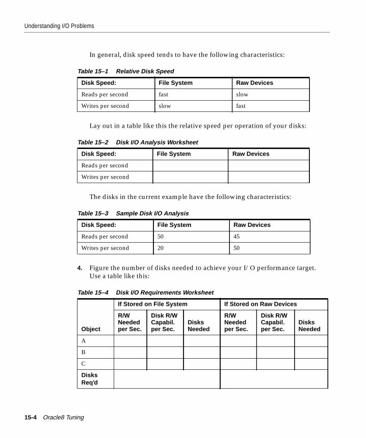
Understanding I/O Problems
In general, disk speed tends to have the following characteristics:
Lay out in a table like this the relative speed per operation of your disks:
The disks in the current example have the following characteristics:
4. Figure the number of disks needed to achieve your I/O performance target.Use a table like this:
Table 15–1 Relative Disk Speed
Disk Speed: File System Raw Devices
Reads per second fast slow
Writes per second slow fast
Table 15–2 Disk I/O Analysis Worksheet
Disk Speed: File System Raw Devices
Reads per second
Writes per second
Table 15–3 Sample Disk I/O Analysis
Disk Speed: File System Raw Devices
Reads per second 50 45
Writes per second 20 50
Table 15–4 Disk I/O Requirements Worksheet
Object
If Stored on File System If Stored on Raw Devices
R/WNeededper Sec.
Disk R/WCapabil.per Sec.
DisksNeeded
R/WNeededper Sec.
Disk R/WCapabil.per Sec.
DisksNeeded
A
B
C
DisksReq’d
15-4 Oracle8 Tuning
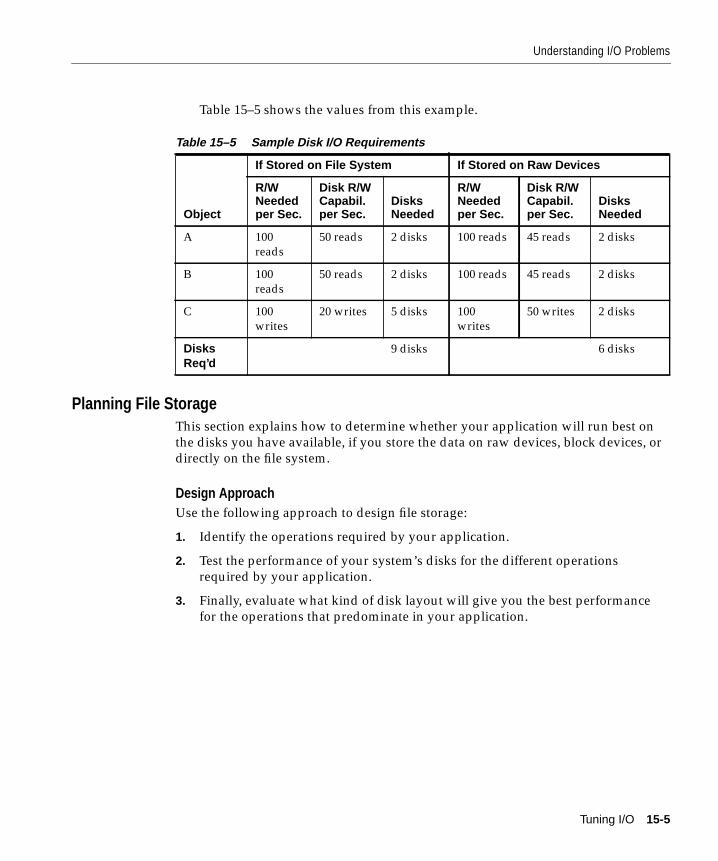
Understanding I/O Problems
Table 15–5 shows the values from this example.
Planning File StorageThis section explains how to determine whether your application will run best onthe disks you have available, if you store the data on raw devices, block devices, ordirectly on the file system.
Design ApproachUse the following approach to design file storage:
1. Identify the operations required by your application.
2. Test the performance of your system’s disks for the different operationsrequired by your application.
3. Finally, evaluate what kind of disk layout will give you the best performancefor the operations that predominate in your application.
Table 15–5 Sample Disk I/O Requirements
Object
If Stored on File System If Stored on Raw Devices
R/WNeededper Sec.
Disk R/WCapabil.per Sec.
DisksNeeded
R/WNeededper Sec.
Disk R/WCapabil.per Sec.
DisksNeeded
A 100reads
50 reads 2 disks 100 reads 45 reads 2 disks
B 100reads
50 reads 2 disks 100 reads 45 reads 2 disks
C 100writes
20 writes 5 disks 100writes
50 writes 2 disks
DisksReq’d
9 disks 6 disks
Tuning I/O 15-5
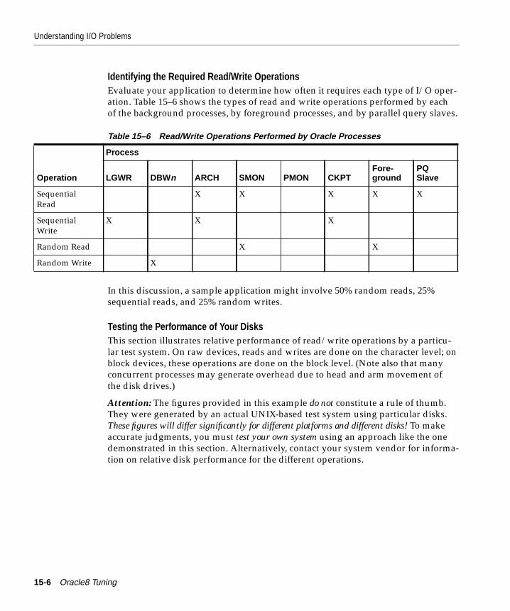
Understanding I/O Problems
Identifying the Required Read/Write OperationsEvaluate your application to determine how often it requires each type of I/O oper-ation. Table 15–6 shows the types of read and write operations performed by eachof the background processes, by foreground processes, and by parallel query slaves.
In this discussion, a sample application might involve 50% random reads, 25%sequential reads, and 25% random writes.
Testing the Performance of Your DisksThis section illustrates relative performance of read/write operations by a particu-lar test system. On raw devices, reads and writes are done on the character level; onblock devices, these operations are done on the block level. (Note also that manyconcurrent processes may generate overhead due to head and arm movement ofthe disk drives.)
Attention: The figures provided in this example do not constitute a rule of thumb.They were generated by an actual UNIX-based test system using particular disks.These figures will differ significantly for different platforms and different disks! To makeaccurate judgments, you must test your own system using an approach like the onedemonstrated in this section. Alternatively, contact your system vendor for informa-tion on relative disk performance for the different operations.
Table 15–6 Read/Write Operations Performed by Oracle Processes
Operation
Process
LGWR DBWn ARCH SMON PMON CKPTFore-ground
PQSlave
SequentialRead
X X X X X
SequentialWrite
X X X
Random Read X X
Random Write X
15-6 Oracle8 Tuning
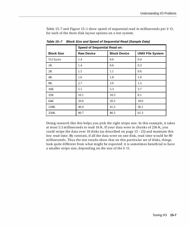
Understanding I/O Problems
Table 15–7 and Figure 15–1 show speed of sequential read in milliseconds per I/O,for each of the three disk layout options on a test system.
Doing research like this helps you pick the right stripe size. In this example, it takesat most 5.3 milliseconds to read 16 K. If your data were in chunks of 256 K, youcould stripe the data over 16 disks (as described on page 15 - 23) and maintain thislow read time. By contrast, if all the data were on one disk, read time would be 80milliseconds. Thus the test results show that on this particular set of disks, thingslook quite different from what might be expected: it is sometimes beneficial to havea smaller stripe size, depending on the size of the I/O.
Table 15–7 Block Size and Speed of Sequential Read (Sample Data)
Block Size
Speed of Sequential Read on:
Raw Device Block Device UNIX File System
512 bytes 1.4 0.6 0.4
1K 1.4 0.6 0.3
2K 1.5 1.1 0.6
4K 1.6 1.8 1.0
8K 2.7 3.0 1.5
16K 5.1 5.3 3.7
32K 10.1 10.3 8.1
64K 20.0 20.3 18.0
128K 40.4 41.3 36.1
256K 80.7 80.3 61.3
Tuning I/O 15-7
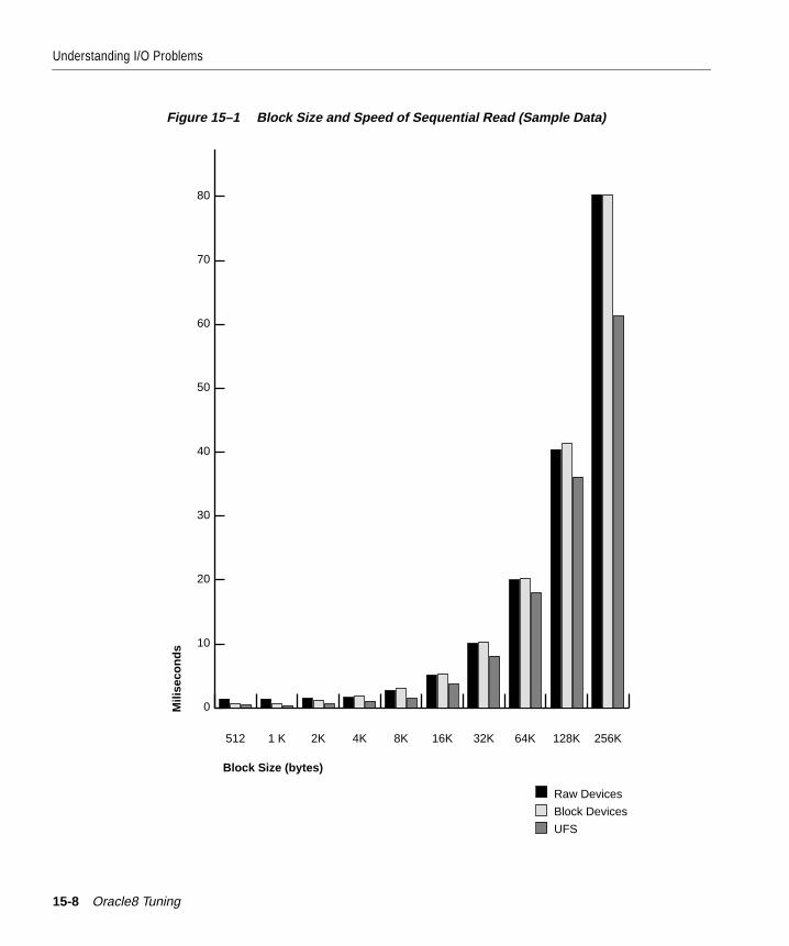
Understanding I/O Problems
Figure 15–1 Block Size and Speed of Sequential Read (Sample Data)
0
10
20
30
40
50
60
70
80
256K128K64K32K16K8K4K2K1 K512
Raw Devices
Block Devices
UFS
Block Size (bytes)
Mili
seco
nd
s
15-8 Oracle8 Tuning

Understanding I/O Problems
Table 15–8 and Figure 15–2 show speed of sequential write in milliseconds per I/O,for each of the three disk layout options on the test system.
Table 15–8 Block Size and Speed of Sequential Write (Sample Data)
Block Size
Speed of Sequential Write on
Raw Device Block Device UNIX File System
512 bytes 11.2 11.8 17.9
1K 11.7 11.9 18.3
2K 11.6 13.0 19.0
4K 12.3 13.8 19.8
8K 13.5 13.8 21.8
16K 16.0 27.8 35.3
32K 19.3 55.6 62.2
64K 31.5 111.1 115.1
128K 62.5 224.5 221.8
256K 115.6 446.1 429.0
Tuning I/O 15-9
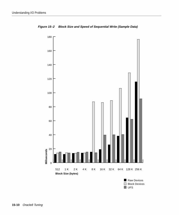
Understanding I/O Problems
Figure 15–2 Block Size and Speed of Sequential Write (Sample Data)
Raw DevicesBlock DevicesUFS
0
20
40
60
80
100
120
140
160
180
256 K128 K64 K32 K16 K8 K4 K2 K1 K512
Block Size (bytes)
Mili
seco
nd
s
15-10 Oracle8 Tuning
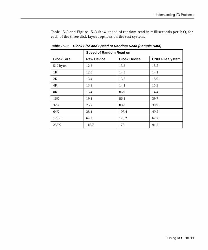
Understanding I/O Problems
Table 15–9 and Figure 15–3 show speed of random read in milliseconds per I/O, foreach of the three disk layout options on the test system.
Table 15–9 Block Size and Speed of Random Read (Sample Data)
Block Size
Speed of Random Read on
Raw Device Block Device UNIX File System
512 bytes 12.3 13.8 15.5
1K 12.0 14.3 14.1
2K 13.4 13.7 15.0
4K 13.9 14.1 15.3
8K 15.4 86.9 14.4
16K 19.1 86.1 39.7
32K 25.7 88.8 39.9
64K 38.1 106.4 40.2
128K 64.3 128.2 62.2
256K 115.7 176.1 91.2
Tuning I/O 15-11
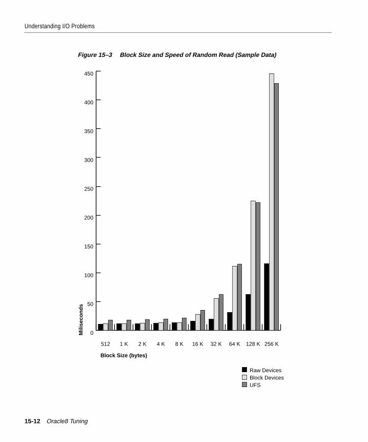
Understanding I/O Problems
Figure 15–3 Block Size and Speed of Random Read (Sample Data)
Raw DevicesBlock DevicesUFS
0
50
100
150
200
250
300
350
400
450
256 K128 K64 K32 K16 K8 K4 K2 K1 K512
Block Size (bytes)
Mili
seco
nd
s
15-12 Oracle8 Tuning
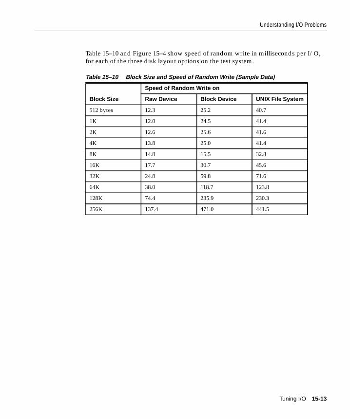
Understanding I/O Problems
Table 15–10 and Figure 15–4 show speed of random write in milliseconds per I/O,for each of the three disk layout options on the test system.
Table 15–10 Block Size and Speed of Random Write (Sample Data)
Block Size
Speed of Random Write on
Raw Device Block Device UNIX File System
512 bytes 12.3 25.2 40.7
1K 12.0 24.5 41.4
2K 12.6 25.6 41.6
4K 13.8 25.0 41.4
8K 14.8 15.5 32.8
16K 17.7 30.7 45.6
32K 24.8 59.8 71.6
64K 38.0 118.7 123.8
128K 74.4 235.9 230.3
256K 137.4 471.0 441.5
Tuning I/O 15-13
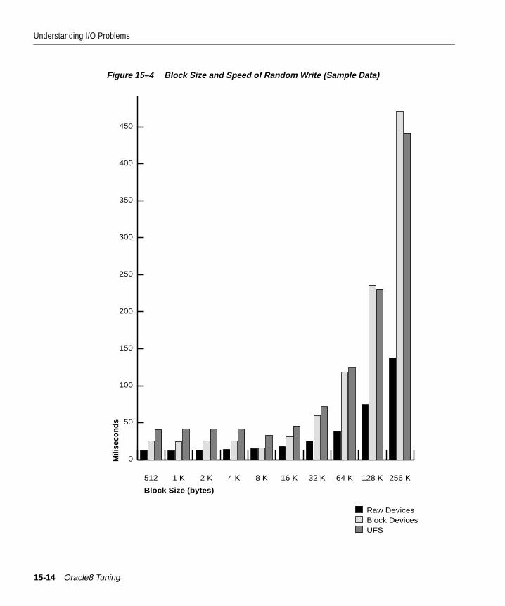
Understanding I/O Problems
Figure 15–4 Block Size and Speed of Random Write (Sample Data)
Raw DevicesBlock DevicesUFS
0
50
100
150
200
250
300
350
400
450
256 K128 K64 K32 K16 K8 K4 K2 K1 K512
Block Size (bytes)
Mili
seco
nds
15-14 Oracle8 Tuning
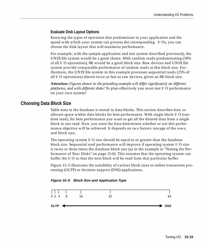
Understanding I/O Problems
Evaluate Disk Layout OptionsKnowing the types of operation that predominate in your application and thespeed with which your system can process the corresponding I/Os, you canchoose the disk layout that will maximize performance.
For example, with the sample application and test system described previously, theUNIX file system would be a good choice. With random reads predominating (50%of all I/O operations), 8K would be a good block size. Raw devices and UNIX filesystem provide comparable performance of random reads at this block size. Fur-thermore, the UNIX file system in this example processes sequential reads (25% ofall I/O operations) almost twice as fast as raw devices, given an 8K block size.
Attention: Figures shown in the preceding example will differ significantly on differentplatforms, and with different disks! To plan effectively you must test I/O performanceon your own system!
Choosing Data Block SizeTable data in the database is stored in data blocks. This section describes how toallocate space within data blocks for best performance. With single block I/O (ran-dom read), for best performance you want to get all the desired data from a singleblock in one read. How you store the data determines whether or not this perfor-mance objective will be achieved. It depends on two factors: storage of the rows,and block size.
The operating system I/O size should be equal to or greater than the databaseblock size. Sequential read performance will improve if operating system I/O sizeis twice or three times the database block size (as in the example in "Testing the Per-formance of Your Disks" on page 15-6). This assumes that the operating system canbuffer the I/O so that the next block will be read from that particular buffer.
Figure 15–5 illustrates the suitability of various block sizes to online transaction pro-cessing (OLTP) or decision support (DSS) applications.
Figure 15–5 Block Size and Application Type
0 2 4 8 16 32 64
OLTP DSS
Tuning I/O 15-15

Understanding I/O Problems
See Also: Your Oracle platform-specific documentation for information on the mini-mum and maximum block size on your platform.
Block Size Advantages and DisadvantagesThis section describes advantages and disadvantages of different block sizes.
Evaluating Device BandwidthThe number of I/Os a disk can perform depends on whether the operationsinvolve reading or writing to objects stored on raw devices or on the file system.This affects the number of disks you must use to achieve the desired level of perfor-mance.
Table 15–11 Block Size Advantages and Disadvantages
Block Size Advantages Disadvantages
Small (2K-4K)Reduces block contention.
Good for small rows, or lots of randomaccess.
Has relatively large overhead.
You may end up storing only a smallnumber of rows, depending on the size ofthe row.
Medium (8K) If rows are of medium size, you can bringa number of rows into the buffer cachewith a single I/O. With 2K or 4K blocksize, you may only bring in a single row.
Space in the buffer cache will be wasted ifyou are doing random access to smallrows and have a large block size. Forexample, with an 8K block size and 50Brow size, you would be wasting 7,950B inthe buffer cache when doing randomaccess.
Large (16K-32K) There is relatively less overhead, thusmore room to store useful data.
Good for sequential access, or very largerows.
Large block size is not good for indexblocks used in an OLTP type environ-ment, because they increase block conten-tion on the index leaf blocks.
15-16 Oracle8 Tuning
How to Detect I/O Problems
How to Detect I/O ProblemsIf you suspect a problem with I/O usage, you must evaluate two areas:
■ Checking System I/O Utilization
■ Checking Oracle I/O Utilization
Oracle compiles file I/O statistics that reflect disk access to database files. Note,however, that these statistics report only the I/O utilization of Oracle sessions—yetevery process running on your system affects the available I/O resources. Tuningnon-Oracle factors can thus result in better Oracle performance.
Checking System I/O UtilizationUse operating system monitoring tools to determine what processes are running onthe system as a whole, and to monitor disk access to all files. Remember that disksholding datafiles and redo log files may also hold files that are not related to Ora-cle. Try to reduce any heavy access to disks that contain database files. Access tonon-Oracle files can be monitored only through operating system facilities ratherthan through the V$FILESTAT table.
Tools such as sar -d on many UNIX systems enable you to examine the iostat I/Ostatistics for your entire system. (Some UNIX-based platforms have an iostat com-mand.) On NT systems, use Performance Monitor.
Attention: For information on other platforms, please check your operating systemdocumentation.
See Also: Oracle platform-specific documentation.
Tuning I/O 15-17
How to Detect I/O Problems
Checking Oracle I/O UtilizationThis section identifies the views and processes that provide Oracle I/O statistics,and shows how to check statistics using V$FILESTAT.
Which Dynamic Performance Tables Contain I/O StatisticsTable 15–12 shows dynamic performance tables to check for I/O statistics relatingto Oracle database files, log files, archive files, and control files.
Which Processes Reflect Oracle File I/OTable 15–13 lists processes whose statistics reflect I/O throughput for the differentOracle file types.
V$SYSTEM_EVENT, for example, shows the total number of I/Os and averageduration, by type of I/O. You can thus determine which types of I/O are too slow.If there are Oracle-related I/O problems, tune them. But if your process is not con-suming the available I/O resources, then some other process is. Go back to the sys-tem to identify the process that is using up so much I/O, and determine why. See ifyou can tune this process.
Table 15–12 Where to Find Statistics about Oracle Files
File Type Where to Find Statistics
Database Files V$FILESTAT
Log Files V$SYSSTAT, V$SYSTEM_EVENT, V$SESSION_EVENT
Archive Files V$SYSTEM_EVENT, V$SESSION_EVENT
Control Files V$SYSTEM_EVENT, V$SESSION_EVENT
Table 15–13 File Throughput Statistics for Oracle Processes
File
Process
LGWR DBWn ARCH SMON PMON CKPTFore-ground
PQSlave
Database Files X X X X X X
Log Files X
Archive Files X
Control Files X X X X X X X X
15-18 Oracle8 Tuning
How to Detect I/O Problems
Note: Different types of I/O in Oracle require different tuning approaches. TuningI/O for data warehousing applications that perform large sequential reads is differ-ent from tuning I/O for OLTP applications that perform random reads and writes.See also "Planning File Storage" on page 15-5.
How to Check Oracle Datafile I/O with V$FILESTATExamine disk access to database files through the dynamic performance tableV$FILESTAT. This view shows the following information for database I/O (but notfor log file I/O):
■ number of physical reads and writes
■ number of blocks read and written
■ total I/O time for reads and writes
By default, this table is available only to the user SYS and to users granted SELECTANY TABLE system privilege, such as SYSTEM. The following column valuesreflect the number of disk accesses for each datafile:
Use the following query to monitor these values over some period of time whileyour application is running:
SELECT name, phyrds, phywrts FROM v$datafile df, v$filestat fs WHERE df.file# = fs.file#;
This query also retrieves the name of each datafile from the dynamic performancetable V$DATAFILE. Sample output might look like this:
NAME PHYRDS PHYWRTS-------------------------------------------- ---------- ----------/oracle/ora70/dbs/ora_system.dbf 7679 2735/oracle/ora70/dbs/ora_temp.dbf 32 546
The PHYRDS and PHYWRTS columns of V$FILESTAT can also be obtainedthrough SNMP.
The total I/O for a single disk is the sum of PHYRDS and PHYWRTS for all thedatabase files managed by the Oracle instance on that disk. Determine this valuefor each of your disks. Also determine the rate at which I/O occurs for each disk by
PHYRDS The number of reads from each database file.
PHYWRTS The number of writes to each database file.
Tuning I/O 15-19

How to Solve I/O Problems
dividing the total I/O by the interval of time over which the statistics were col-lected.
How to Solve I/O ProblemsThe rest of this chapter describes various techniques of solving I/O problems:
■ Reducing Disk Contention by Distributing I/O
■ Striping Disks
■ Avoiding Dynamic Space Management
■ Tuning Sorts
■ Tuning Checkpoints
■ Tuning LGWR and DBWn I/O
■ Configuring the Large Pool
15-20 Oracle8 Tuning
Reducing Disk Contention by Distributing I/O
Reducing Disk Contention by Distributing I/OThis section describes how to reduce disk contention.
■ What Is Disk Contention?
■ Separating Datafiles and Redo Log Files
■ Striping Table Data
■ Separating Tables and Indexes
■ Reducing Disk I/O Unrelated to Oracle
What Is Disk Contention?Disk contention occurs when multiple processes try to access the same disk simulta-neously. Most disks have limits on both the number of accesses and the amount ofdata they can transfer per second. When these limits are reached, processes mayhave to wait to access the disk.
In general, consider the statistics in the V$FILESTAT table and your operating sys-tem facilities. Consult your hardware documentation to determine the limits on thecapacity of your disks. Any disks operating at or near full capacity are potentialsites for disk contention. For example, 40 or more I/Os per second is excessive formost disks on VMS or UNIX operating systems.
To reduce the activity on an overloaded disk, move one or more of its heavilyaccessed files to a less active disk. Apply this principle to each of your disks untilthey all have roughly the same amount of I/O. This is referred to as distributing I/O.
Separating Datafiles and Redo Log FilesOracle processes constantly access datafiles and redo log files. If these files are oncommon disks, there is potential for disk contention. Place each datafile on a sepa-rate disk. Multiple processes can then access different files concurrently withoutdisk contention.
Place each set of redo log files on a separate disk with no other activity. Redo logfiles are written by the Log Writer process (LGWR) when a transaction is commit-ted. Information in a redo log file is written sequentially. This sequential writingcan take place much faster if there is no concurrent activity on the same disk. Dedi-cating a separate disk to redo log files usually ensures that LGWR runs smoothlywith no further tuning attention. Performance bottlenecks related to LGWR arerare. For information on tuning LGWR, see the section "Detecting Contention forRedo Log Buffer Latches" on page 18-13.
Tuning I/O 15-21
Reducing Disk Contention by Distributing I/O
Note: Mirroring redo log files, or maintaining multiple copies of each redo log fileon separate disks, does not slow LGWR considerably. LGWR writes to each disk inparallel and waits until each part of the parallel write is complete. Since the timerequired for your operating system to perform a single-disk write may vary,increasing the number of copies increases the likelihood that one of the single-diskwrites in the parallel write will take longer than average. A parallel write will nottake longer than the longest possible single-disk write. There may also be someoverhead associated with parallel writes on your operating system.
Dedicating separate disks and mirroring redo log files are important safety precau-tions. Dedicating separate disks to datafiles and redo log files ensures that the data-files and the redo log files cannot both be lost in a single disk failure. Mirroringredo log files ensures that a redo log file cannot be lost in a single disk failure.
Striping Table DataStriping, or spreading a large table’s data across separate datafiles on separatedisks, can also help to reduce contention. This strategy is fully discussed in the sec-tion "Striping Disks" on page 15-23.
Separating Tables and IndexesIt is not necessary to separate a frequently used table from its index. During thecourse of a transaction, the index is read first, and then the table is read. Becausethese I/Os occur sequentially, the table and index can be stored on the same diskwithout contention.
Reducing Disk I/O Unrelated to OracleIf possible, eliminate I/O unrelated to Oracle on disks that contain database files.This measure is especially helpful in optimizing access to redo log files. Not onlydoes this reduce disk contention, it also allows you to monitor all activity on suchdisks through the dynamic performance table V$FILESTAT.
15-22 Oracle8 Tuning
Striping Disks
Striping DisksThis section describes:
■ What Is Striping?
■ I/O Balancing and Striping
■ How to Stripe Disks Manually
■ How to Stripe Disks with Operating System Software
■ How to Do Hardware Striping with RAID
What Is Striping?“Striping” is the practice of dividing a large table’s data into small portions andstoring these portions in separate datafiles on separate disks. This permits multipleprocesses to access different portions of the table concurrently without disk conten-tion. Striping is particularly helpful in optimizing random access to tables withmany rows. Striping can either be done manually (described below), or throughoperating system striping utilities.
I/O Balancing and StripingBenchmark tuners in the past tried hard to ensure that the I/O load was evenly bal-anced across the available devices. Currently, operating systems are providing theability to stripe a heavily used container file across many physical devices. How-ever, such techniques are productive only where the load redistribution eliminatesor reduces some form of queue.
If I/O queues exist or are suspected, then load distribution across the availabledevices is a natural tuning step. Where larger numbers of physical drives are avail-able, consider dedicating two drives to carrying redo logs (two because redo logsshould always be mirrored either by the operating system or using Oracle redo loggroup features). Since redo logs are written serially, any drive dedicated to redo logactivity will normally require very little head movement. This will significantlyspeed up log writing.
When archiving, it is beneficial to use extra disks so that LGWR and ARCH do notcompete for the same read/write head. This is achieved by placing logs on alternat-ing drives.
Note that mirroring can also be a cause of I/O bottlenecks. The process of writingto each mirror is normally done in parallel, and does not cause a bottleneck. How-ever, if each mirror is striped differently, then the I/O is not completed until the
Tuning I/O 15-23
Striping Disks
slowest member is finished. To avoid I/O problems, striping should be done on thesame number of disks as the data itself.
For example, if you have 160K of data striped over 8 disks, but the data is mirroredonto only one disk, then regardless of how quickly the data is processed on the 8disks, the I/O is not completed until 160K has been written onto the mirror disk. Itmight thus take 20.48 milliseconds to write the database, but 137 milliseconds towrite the mirror.
How to Stripe Disks ManuallyTo stripe disks manually, you need to relate the object’s storage requirements to itsI/O requirements.
1. Begin by evaluating the object’s disk storage requirements. You need to know
■ the size of the object
■ the size of the disk
For example, if the object requires 5G in Oracle storage space, you would needone 5G disk or two 4G disks to accommodate it. On the other hand, if the sys-tem is configured with 1G or 2G disks, the object may require 5 or 3 disks,respectively.
2. Compare to this the application’s I/O requirements, as described in "AnalyzingI/O Requirements" on page 15-3. You must take the larger of the storagerequirement and the I/O requirement.
For example, if the storage requirement is 5 disks (1G each), and the I/Orequirement is 2 disks, then your application requires the higher value: 5 disks.
3. Create a tablespace with the CREATE TABLESPACE command. Specify thedatafiles in the DATAFILE clause. Each of the files should be on a different disk.
CREATE TABLESPACE stripedtabspace DATAFILE ’file_on_disk_1’ SIZE 1GB, ’file_on_disk_2’ SIZE 1GB, ’file_on_disk_3’ SIZE 1GB, ’file_on_disk_4’ SIZE 1GB, ’file_on_disk_5’ SIZE 1GB;
4. Then create the table with the CREATE TABLE command. Specify the newlycreated tablespace in the TABLESPACE clause.
Also specify the size of the table extents in the STORAGE clause. Store eachextent in a separate datafile. The table extents should be slightly smaller than
15-24 Oracle8 Tuning
Striping Disks
the datafiles in the tablespace to allow for overhead. For example, when prepar-ing for datafiles of 1G (1024MB), you can set the table extents to be 1023MB:
CREATE TABLE stripedtab ( col_1 NUMBER(2), col_2 VARCHAR2(10) ) TABLESPACE stripedtabspace STORAGE ( INITIAL 1023MB NEXT 1023MB MINEXTENTS 5 PCTINCREASE 0 );
(Alternatively, you can stripe a table by entering an ALTER TABLE ALLOCATEEXTENT statement, with a DATAFILE ’size’ SIZE clause.)
These steps result in the creation of table STRIPEDTAB. STRIPEDTAB has 5 initialextents, each of size 1023MB. Each extent takes up one of the datafiles named in theDATAFILE clause of the CREATE TABLESPACE statement. Each of these files is ona separate disk. The 5 extents are all allocated immediately, because MINEXTENTSis 5.
See Also: Oracle8 SQL Reference for more information on MINEXTENTS and theother storage parameters.
How to Stripe Disks with Operating System SoftwareAn alternative to striping disks manually, you can use operating system stripingsoftware, such as a logical volume manager (LVM), to stripe disks. With stripingsoftware, the biggest concern is choosing the right stripe size. This depends on Ora-cle block size and type of disk access.
In striping, uniform access to the data is assumed. If the stripe size is too big youcan end up with a hot spot on one disk or on a small number of disks. You canavoid this problem by making the stripe size smaller, thus spreading the data overmore disks.
Table 15–14 Minimum Stripe Size
Disk Access Minimum Stripe Size
Random reads andwrites
The minimum stripe size is twice the Oracle block size.
Sequential reads The minimum stripe size is twice the value ofDB_FILE_MULTIBLOCK_READ_COUNT.
Tuning I/O 15-25
Avoiding Dynamic Space Management
Consider an example in which 100 rows of fixed size are evenly distributed over 5disks, with each disk containing 20 sequential rows. If access is needed only torows 35 through 55, then only 2 disks must handle all the I/O. At this rate, the sys-tem cannot achieve the desired level of performance.
You can correct this problem by spreading the rows of interest across more disks. Inthe current example, if there were two rows per block, then we could place rows 35and 36 on the same disk, and rows 37 and 38 on a different disk. Taking thisapproach, we could spread the data of interest over all the disks and I/O through-put would be much improved.
How to Do Hardware Striping with RAIDRedundant arrays of inexpensive disks (RAID) can offer significant advantages intheir failure resilience features. They also permit striping to be achieved quite eas-ily, but do not appear to provide any significant performance advantage. In fact,they may impose a higher cost in I/O overhead.
In some instances, performance can be improved by not using the full features ofRAID technology. In other cases, RAID technology’s resilience to single componentfailure may justify its cost in terms of performance.
Avoiding Dynamic Space ManagementWhen an object such as a table or rollback segment is created, space is allocated inthe database for the data. This space is called a segment. If subsequent databaseoperations cause the data to grow and exceed the space allocated, Oracle extendsthe segment. Dynamic extension can reduce performance. This section discusses
■ Detecting Dynamic Extension
■ Allocating Extents
■ Evaluating Unlimited Extents
■ Evaluating Multiple Extents
■ Avoiding Dynamic Space Management in Rollback Segments
■ Reducing Migrated and Chained Rows
■ Modifying the SQL.BSQ File
15-26 Oracle8 Tuning
Avoiding Dynamic Space Management
Detecting Dynamic ExtensionDynamic extension causes Oracle to execute SQL statements in addition to thoseSQL statements issued by user processes. These SQL statements are called recursivecalls because Oracle issues these statements itself. Recursive calls are also generatedby these activities:
■ misses on the data dictionary cache
■ firing of database triggers
■ execution of Data Definition Language statements
■ execution of SQL statements within stored procedures, functions, packages,and anonymous PL/SQL blocks
■ enforcement of referential integrity constraints
Examine the RECURSIVE CALLS statistic through the dynamic performance tableV$SYSSTAT. By default, this table is available only to the user SYS and to usersgranted the SELECT ANY TABLE system privilege, such as SYSTEM. Monitor thisstatistic over some period of time while your application is running, with thisquery:
SELECT name, valueFROM v$sysstatWHERE name = ’recursive calls’;
The output of this query might look like this:
NAME VALUE------------------------------------------------------- ----------recursive calls 626681
If Oracle continues to make excessive recursive calls while your application is run-ning, determine whether these recursive calls are due to one of the activities thatgenerate recursive calls other than dynamic extension. If you determine that theserecursive calls are caused by dynamic extension, you should try to reduce thisextension by allocating larger extents.
Tuning I/O 15-27
Avoiding Dynamic Space Management
Allocating ExtentsFollow these steps to avoid dynamic extension:
1. Determine the maximum size of your object. For formulas to estimate howmuch space to allow for a table, see the Oracle8 Administrator’s Guide.
2. Choose storage parameter values so that Oracle allocates extents large enoughto accommodate all of your data when you create the object.
Larger extents tend to benefit performance for these reasons:
■ Blocks in a single extent are contiguous, so one large extent is more contiguousthan multiple small extents. Oracle can read one large extent from disk withfewer multiblock reads than would be required to read many small extents.
■ Segments with larger extents are less likely to be extended.
However, since large extents require more contiguous blocks, Oracle may have diffi-culty finding enough contiguous space to store them. To determine whether to allo-cate few large extents or many small extents, consider the benefits and drawbacksof each in light of your plans for the growth and use of your tables.
Automatically resizable datafiles can also cause a problem with dynamic extension.Avoid using the automatic extension. Instead, manually allocate more space to adatafile during times when the system is relatively inactive.
15-28 Oracle8 Tuning
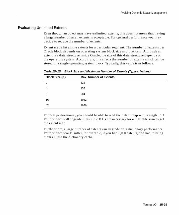
Avoiding Dynamic Space Management
Evaluating Unlimited ExtentsEven though an object may have unlimited extents, this does not mean that havinga large number of small extents is acceptable. For optimal performance you maydecide to reduce the number of extents.
Extent maps list all the extents for a particular segment. The number of extents perOracle block depends on operating system block size and platform. Although anextent is a data structure inside Oracle, the size of this data structure depends onthe operating system. Accordingly, this affects the number of extents which can bestored in a single operating system block. Typically, this value is as follows:
For best performance, you should be able to read the extent map with a single I/O.Performance will degrade if multiple I/Os are necessary for a full table scan to getthe extent map.
Furthermore, a large number of extents can degrade data dictionary performance.Performance would suffer, for example, if you had 8,000 extents, and had to bringthem all into the dictionary cache.
Table 15–15 Block Size and Maximum Number of Extents (Typical Values)
Block Size (K) Max. Number of Extents
2 121
4 255
8 504
16 1032
32 2070
Tuning I/O 15-29
Avoiding Dynamic Space Management
Evaluating Multiple ExtentsThis section explains various ramifications of the use of multiple extents.
You cannot put very large segments into single extents because of file size and filesystem size limitations. When you enable segments to allocate new extents overtime, you can take advantage of faster, less expensive disks. Note also:
■ For a table that is never full-table scanned, it makes no difference in terms ofquery performance whether the table has one extent or multiple extents.
■ The performance of searches using an index is not affected by the index havingone extent or multiple extents.
■ Using more than one extent in a table, cluster, or temporary segment does notmaterially affect the performance of full scans on an operational multi-user sys-tem.
■ Using more than one extent in a table, cluster, or temporary segment does notmaterially affect the performance of full scans on a dedicated single-user batchprocessing system if the extents are properly sized, and if the application isdesigned to avoid expensive DDL operations.
■ If extent sizes are appropriately matched to the I/O size, the performance costof having many extents in a segment will be minimized.
■ For rollback segments, many extents are preferable to few extents. Havingmany extents reduces the number of recursive SQL calls to perform dynamicextent allocations on the segments.
Avoiding Dynamic Space Management in Rollback SegmentsThe size of rollback segments can affect performance. Rollback segment size isdetermined by the rollback segment’s storage parameter values. Your rollback seg-ments must be large enough to hold the rollback entries for your transactions. Aswith other objects, you should avoid dynamic space management in rollback seg-ments.
Use the SET TRANSACTION command to assign transactions to rollback segmentsof the appropriate size based on the recommendations in the following sections. Ifyou do not explicitly assign a transaction to a rollback segment, Oracle automati-cally assigns it to a rollback segment.
For example, the following statement assigns the current transaction to the rollbacksegment OLTP_13:
SET TRANSACTION USE ROLLBACK SEGMENT oltp_13
15-30 Oracle8 Tuning
Avoiding Dynamic Space Management
Warning: If you are running multiple concurrent copies of the same application, becareful not to assign the transactions for all copies to the same rollback segment.This leads to contention for that rollback segment.
Also monitor the shrinking, or dynamic deallocation, of rollback segments basedon the OPTIMAL storage parameter. For information on choosing values for thisparameter, monitoring rollback segment shrinking, and adjusting OPTIMALaccordingly, see Oracle8 Administrator’s Guide.
For Long QueriesAssign large rollback segments to transactions that modify data which is concur-rently selected by long queries. Such queries may require access to rollback seg-ments to reconstruct a read-consistent version of the modified data. The rollbacksegments must be large enough to hold all the rollback entries for the data whilethe query is running.
For Long TransactionsAssign large rollback segments to transactions that modify large amounts of data.A large rollback segment can improve the performance of such a transaction. Suchtransactions generate large rollback entries. If a rollback entry does not fit into arollback segment, Oracle extends the segment. Dynamic extension reduces perfor-mance and should be avoided whenever possible.
For OLTP TransactionsOLTP applications are characterized by frequent concurrent transactions, each ofwhich modifies a small amount of data. Assign to OLTP transactions to small roll-back segments, provided that their data is not concurrently queried. Small rollbacksegments are more likely to remain stored in the buffer cache where they can beaccessed quickly. A typical OLTP rollback segment might have 2 extents, eachapproximately 10 kilobytes in size. To best avoid contention, create many rollbacksegments and assign each transaction to its own rollback segment.
Tuning I/O 15-31
Avoiding Dynamic Space Management
Reducing Migrated and Chained RowsIf an UPDATE statement increases the amount of data in a row so that the row nolonger fits in its data block, Oracle tries to find another block with enough freespace to hold the entire row. If such a block is available, Oracle moves the entirerow to the new block. This is called migrating a row. If the row is too large to fit intoany available block, Oracle splits the row into multiple pieces and stores each piecein a separate block. This is called chaining a row. Rows can also be chained whenthey are inserted.
Dynamic space management, especially migration and chaining, is detrimental toperformance:
■ UPDATE statements that cause migration and chaining perform poorly.
■ Queries that select migrated or chained rows must perform more I/O.
You can identify migrated and chained rows in a table or cluster by using the ANA-LYZE command with the LIST CHAINED ROWS option. This command collectsinformation about each migrated or chained row and places this information into aspecified output table. The definition of a sample output table namedCHAINED_ROWS appears in a SQL script available on your distribution medium.The common name of this script is UTLCHAIN.SQL, although its exact name andlocation may vary depending on your operating system. Your output table musthave the same column names, datatypes, and sizes as the CHAINED_ROWS table.
To reduce migrated and chained rows in an existing table, follow these steps:
1. Use the ANALYZE command to collect information about migrated andchained rows. For example:
ANALYZE TABLE order_hist LIST CHAINED ROWS;
2. Query the output table:
SELECT * FROM chained_rows WHERE table_name = ’ORDER_HIST’;
OWNER_NAME TABLE_NAME CLUST... HEAD_ROWID TIMESTAMP---------- ---------- -----... ------------------ ---------SCOTT ORDER_HIST ... AAAAluAAHAAAAA1AAA 04-MAR-96SCOTT ORDER_HIST ... AAAAluAAHAAAAA1AAB 04-MAR-96SCOTT ORDER_HIST ... AAAAluAAHAAAAA1AAC 04-MAR-96
The output lists all rows that are either migrated or chained.
15-32 Oracle8 Tuning
Avoiding Dynamic Space Management
3. If the output table shows that you have many migrated or chained rows, youcan eliminate migrated rows with the following steps:
a. Create an intermediate table with the same columns as the existing table tohold the migrated and chained rows:
CREATE TABLE int_order_hist AS SELECT * FROM order_hist WHERE ROWID IN (SELECT head_rowid FROM chained_rows WHERE table_name = ’ORDER_HIST’);
b. Delete the migrated and chained rows from the existing table:
DELETE FROM order_hist WHERE ROWID IN (SELECT head_rowid FROM chained_rows WHERE table_name = ’ORDER_HIST’);
c. Insert the rows of the intermediate table into the existing table:
INSERT INTO order_hist SELECT * FROM int_order_hist;
d. Drop the intermediate table:
DROP TABLE int_order_history;
4. Delete the information collected in step 1 from the output table:
DELETE FROM chained_rows WHERE table_name = ’ORDER_HIST’;
5. Use the ANALYZE command again and query the output table.
6. Any rows that appear in the output table are chained. You can eliminatechained rows only by increasing your data block size. It may not be possible toavoid chaining in all situations. Chaining is often unavoidable with tables thathave a LONG column or long CHAR or VARCHAR2 columns.
Retrieval of migrated rows is resource intensive; therefore, all tables subject toUPDATE should have their distributed free space set to allow enough space withinthe block for the likely update.
Tuning I/O 15-33
Avoiding Dynamic Space Management
You can detect migrated or chained rows by checking the “table fetch continuedrow” statistic in V$SYSSTAT. Increase PCTFREE to avoid migrated rows. If youleave more free space available in the block, the row will have room to grow. Youcan also reorganize (re-create) tables and indexes with a high deletion rate.
Note: PCTUSED is not the opposite of PCTFREE; it concerns space management.
See Also: Oracle8 Concepts for more information.
Modifying the SQL.BSQ FileThe SQL.BSQ file is run when you issue the CREATE DATABASE statement. Thisfile contains the actual table definitions that make up the Oracle Server. The viewsthat you use as a DBA are based on these tables. Oracle Corporation recommendsthat users strictly limit their modifications to SQL.BSQ.
■ If necessary, you can increase the value of the following storage parameters:INITIAL, NEXT, MINEXTENTS, MAXEXTENTS, PCTINCREASE, FREELISTS,FREELIST GROUPS, and OPTIMAL.
■ With the exception of PCTINCREASE, you should not decrease the setting of astorage parameter to a value below the default. (If the value of MAXEXTENTSis large, you can make PCTINCREASE small—or even zero.)
■ No other changes to SQL.BSQ are supported. In particular, you should not add,drop, or rename a column.
Note: Oracle may add, delete, or change internal data dictionary tables from releaseto release. For this reason, any modifications you make will not be carried forwardwhen the dictionary is migrated to later releases.
See Also: Oracle8 SQL Reference for complete information about these parameters.
15-34 Oracle8 Tuning
Tuning Sorts
Tuning SortsThere is a trade-off between performance and memory usage. For best perfor-mance, most sorts should occur in memory; sorts to disk affect performance. If thesort area size is too big, too much memory may be utilized; if the sort area size istoo small, many sorts to disk may result, with correspondingly worse performance.This section describes:
■ Sorting to Memory
■ If You Do Sort to Disk
■ Optimizing Sort Performance with Temporary Tablespaces
■ Using NOSORT to Create Indexes Without Sorting
■ GROUP BY NOSORT
■ Optimizing Large Sorts with SORT_DIRECT_WRITES
Tuning I/O 15-35
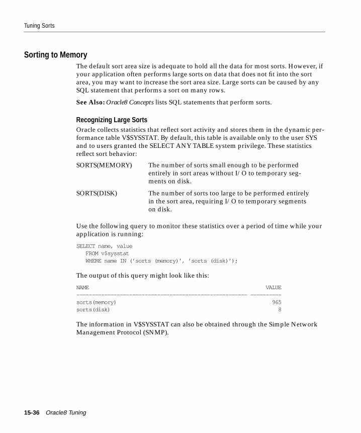
Tuning Sorts
Sorting to MemoryThe default sort area size is adequate to hold all the data for most sorts. However, ifyour application often performs large sorts on data that does not fit into the sortarea, you may want to increase the sort area size. Large sorts can be caused by anySQL statement that performs a sort on many rows.
See Also: Oracle8 Concepts lists SQL statements that perform sorts.
Recognizing Large SortsOracle collects statistics that reflect sort activity and stores them in the dynamic per-formance table V$SYSSTAT. By default, this table is available only to the user SYSand to users granted the SELECT ANY TABLE system privilege. These statisticsreflect sort behavior:
Use the following query to monitor these statistics over a period of time while yourapplication is running:
SELECT name, value FROM v$sysstat WHERE name IN (’sorts (memory)’, ’sorts (disk)’);
The output of this query might look like this:
NAME VALUE------------------------------------------------------- ----------sorts(memory) 965sorts(disk) 8
The information in V$SYSSTAT can also be obtained through the Simple NetworkManagement Protocol (SNMP).
SORTS(MEMORY) The number of sorts small enough to be performedentirely in sort areas without I/O to temporary seg-ments on disk.
SORTS(DISK) The number of sorts too large to be performed entirelyin the sort area, requiring I/O to temporary segmentson disk.
15-36 Oracle8 Tuning
Tuning Sorts
Increasing SORT_AREA_SIZE to Avoid Sorting to DiskSORT_AREA_SIZE is a dynamically modifiable initialization parameter that speci-fies the maximum amount of program global area (PGA) memory to use for a sort.There is a trade-off between SORT_AREA_SIZE and PGA.
If a significant number of sorts require disk I/O to temporary segments, then yourapplication’s performance may benefit from increasing the size of the sort area. Inthis case, increase the value of SORT_AREA_SIZE. The maximum value of thisparameter depends on your operating system. You need to determine how large aSORT_AREA_SIZE makes sense. If it is big enough, most sorts should not go todisk (unless, for example, you are sorting a 10 gigabyte table). If the sort does notgo to disk, you have the option of writing or not writing to the buffer cache.
See Also: "Optimizing Large Sorts with SORT_DIRECT_WRITES" on page 15-40"SORT_AREA_SIZE" on page 19-9
Performance Benefits of Large Sort AreasIncreasing the sort area increases the size of each run and decreases the total num-ber of runs. Reducing the total number of runs may reduce the number of mergesOracle must perform to obtain the final sorted result.
Performance Trade-offs for Large Sort AreasIncreasing the size of the sort area causes each Oracle process that sorts to allocatemore memory. This increase reduces the amount of memory available for privateSQL and PL/SQL areas. It can also affect operating system memory allocation andmay induce paging and swapping. Before increasing the size of the sort area, besure enough free memory is available on your operating system to accommodate alarger sort area.
If you increase sort area size, consider decreasing the retained size of the sort area,or the size to which Oracle reduces the sort area if its data is not expected to be ref-erenced soon. To do this, decrease the value of the SORT_AREA_RETAINED_SIZEparameter. A smaller retained sort area reduces memory usage but causes addi-tional I/O to write and read data to and from temporary segments on disk.
If You Do Sort to DiskIf you do sort to disk, make sure that PCTINCREASE is set to zero for thetablespace used for sorting. Also, INITIAL and NEXT should be the same size. Thisreduces fragmentation of the tablespaces used for sorting. You set these parametersusing the STORAGE option of ALTER TABLE. (See Oracle8 Concepts for more infor-mation on PCTINCREASE.)
Tuning I/O 15-37
Tuning Sorts
Optimizing Sort Performance with Temporary TablespacesYou can optimize sort performance by specifying a tablespace as TEMPORARYupon creation (or subsequently altering that tablespace) and performing the sort inthat tablespace. Normally, a sort may require many space allocation calls to allocateand deallocate temporary segments. If a tablespace is specified as TEMPORARY,one sort segment in that tablespace is cached and used for each instance requestinga sort operation. This scheme bypasses the normal space allocation mechanism andcan greatly improve performance of medium-sized sorts that cannot be done com-pletely in memory.
To specify a tablespace as temporary, use the TEMPORARY keyword of the CRE-ATE TABLESPACE or ALTER TABLESPACE commands. TEMPORARY cannot beused with tablespaces that contain permanent objects (such as tables or rollback seg-ments).
The temporary tablespace should be striped over many disks, preferably with someoperating system striping tool. For example, if the temporary tablespace is onlystriped over 2 disks with a maximum of 50 I/Os per second each, then you canonly do 100 I/Os per second. This restriction could become a problem, making sortoperations take a very long time. You could speed up sorts fivefold if you were tostripe the temporary tablespace over 10 disks. This would enable 500 I/Os per sec-ond.
Change the SORT_READ_FAC parameter, which is a ratio describing the amountof time necessary to read a single database block divided by the block transfer rate.The value is operating system specific; the default value is typically 5, but theparameter should usually be set to 16 or 32. This allows the system to read moreblocks per pass from a temporary table. For temporary tablespaces,SORT_READ_FAC plays a role similar to the parameterDB_FILE_MULTIBLOCK_READ_COUNT.
See Also: Oracle8 SQL Reference for more information about the syntax of the CRE-ATE TABLESPACE and ALTER TABLESPACE commands.
15-38 Oracle8 Tuning
Tuning Sorts
Using NOSORT to Create Indexes Without SortingOne cause of sorting is the creation of indexes. Creating an index for a tableinvolves sorting all the rows in the table based on the values of the indexed col-umns. Oracle also allows you to create indexes without sorting. If the rows in thetable are loaded in ascending order, you can create the index faster without sorting.
The NOSORT OptionTo create an index without sorting, load the rows into the table in ascending orderof the indexed column values. Your operating system may provide a sorting utilityto sort the rows before you load them. When you create the index, use theNOSORT option on the CREATE INDEX command. For example, this CREATEINDEX statement creates the index EMP_INDEX on the ENAME column of theEMP table without sorting the rows in the EMP table:
CREATE INDEX emp_index ON emp(ename) NOSORT;
Note: Specifying NOSORT in a CREATE INDEX statement negates the use of PAR-ALLEL INDEX CREATE, even if PARALLEL (DEGREE n) is specified.
When to Use the NOSORT OptionPresorting your data and loading it in order may not always be the fastest way toload a table.
■ If you have a multiple-CPU computer, you may be able to load data fasterusing multiple processors in parallel, each processor loading a different portionof the data. To take advantage of parallel processing, load the data without sort-ing it first. Then create the index without the NOSORT option.
■ If you have a single-CPU computer, you should sort your data before loading,if possible. Then create the index with the NOSORT option.
GROUP BY NOSORTSorting can be avoided when performing a GROUP BY operation when you knowthat the input data is already ordered so that all rows in each group are clumpedtogether. This may be the case, for example, if the rows are being retrieved from anindex that matches the grouped columns, or if a sort-merge join produces the rowsin the right order. ORDER BY sorts can be avoided in the same circumstances.When no sort takes place, the EXPLAIN PLAN output indicates GROUP BYNOSORT.
Tuning I/O 15-39
Tuning Sorts
Optimizing Large Sorts with SORT_DIRECT_WRITESIf memory and temporary space are abundant on your system, and you performmany large sorts to disk, you can set the initialization parameterSORT_DIRECT_WRITES to increase sort performance.
Behavior of SORT_DIRECT_WRITESWhen this parameter is set to TRUE, each sort allocates several large buffers inmemory for direct disk I/O. You can set the initialization parametersSORT_WRITE_BUFFERS and SORT_WRITE_BUFFER_SIZE to control the numberand size of these buffers. The sort will write an entire buffer for each I/O operation.The Oracle process performing the sort writes the sort data directly to the disk,bypassing the buffer cache.
The default value of SORT_DIRECT_WRITES is AUTO. When the parameter isunspecified or set to AUTO, Oracle automatically allocates direct write buffers ifthe SORT_AREA_SIZE is at least ten times the minimum direct write buffer config-uration.
The memory for the direct write buffers is subtracted from the sort area, so the totalamount of memory used for each sort is still SORT_AREA_SIZE. SettingSORT_WRITE_BUFFERS and SORT_WRITE_BUFFER_SIZE has no effect whenSORT_DIRECT_WRITES is AUTO.
Performance Trade-offs of Direct Disk I/O for SortsSetting SORT_DIRECT_WRITES to TRUE causes each Oracle process that sorts toallocate memory in addition to that already allocated for the sort area. The addi-tional memory allocated is calculated as follows:
SORT_WRITE_BUFFERS * SORT_WRITE_BUFFER_SIZE
The minimum direct write configuration on most platforms is two 32K buffers(2 * 32K), so direct write is generally allocated only if the sort area is 640K orgreater. With a sort area smaller than this, direct write will not be performed.
Ensure that your operating system has enough free memory available to accommo-date this increase. Also, sorts that use direct writes tend to consume more tempo-rary segment space on disk.
One way to avoid increasing memory usage is to decrease the sort area by theamount of memory allocated for direct writes. Note that reducing the sort area mayincrease the number of sorts to disk, which will decrease overall performance. Agood rule of thumb is that the total memory allocated for direct write buffersshould be less than one-tenth of the memory allocated for the sort area. If the mini-
15-40 Oracle8 Tuning
Tuning Checkpoints
mum configuration of the direct write buffers is greater than one-tenth of your sortarea, then you should not trade sort area for direct write buffers.
Tuning CheckpointsA checkpoint is an operation that Oracle performs automatically. Checkpoints canmomentarily reduce performance. This section explains:
■ How Checkpoints Affect Performance
■ Choosing Checkpoint Frequency
■ Reducing the Performance Impact of a Checkpoint
How Checkpoints Affect PerformanceCheckpoints affect:
■ recovery time performance
■ run-time performance
Frequent checkpoints can reduce recovery time in the event of an instance failure. Ifcheckpoints are relatively frequent, then relatively few changes to the database aremade between checkpoints. In this case, relatively few changes must be rolled for-ward for recovery.
However, a checkpoint can momentarily reduce run-time performance for these rea-sons:
■ Checkpoints cause DBWn processes to perform I/O.
■ If CKPT is not enabled, checkpoints cause LGWR to update datafiles and maymomentarily prevent LGWR from writing redo entries.
The overhead associated with a checkpoint is usually small and affects perfor-mance only while Oracle performs the checkpoint.
Tuning I/O 15-41
Tuning Checkpoints
Choosing Checkpoint FrequencyChoose a checkpoint frequency based on your performance concerns. If you aremore concerned with efficient run-time performance than recovery time, choose alower checkpoint frequency. If you are more concerned with fast recovery timethan run-time performance, choose a higher checkpoint frequency.
Because checkpoints on log switches are necessary for redo log maintenance, youcannot eliminate checkpoints entirely. However, you can reduce checkpoint fre-quency to a minimum by setting these parameters:
■ Set the value of the LOG_CHECKPOINT_INTERVAL initialization parameter(in multiples of physical block size) to be larger than the size of your largestredo log file.
■ Set the value of the LOG_CHECKPOINT_TIMEOUT initialization parameter to0. This value eliminates time-based checkpoints.
Such settings eliminate all checkpoints except those that occur on log switches.
You can further reduce checkpoints by reducing the frequency of log switches. Toreduce log switches, increase the size of your redo log files so that the files do notfill as quickly.
Reducing the Performance Impact of a CheckpointTo reduce the performance impact of checkpoints, make sure that DBWn pro-cess(es) write enough during periods of normal (nonpeak) activity. DBWn activitysometimes has a pattern of sharp peaks and valleys. If DBWn is tuned to be moreaggressive in writing, then the average level of its activity will be raised, and it willnot fall behind.
DB_BLOCK_CHECKPOINT_BATCH specifies the number of blocks the DBWn pro-cess(es) can write out in one batch as part of a checkpoint. If the internal Oraclewrite batch size is 512 buffers, and DB_BLOCK_CHECKPOINT_BATCH is set to 8,then the checkpoint may take a very long time. Because you only write 8 blocks at atime, the start and end of a checkpoint will take a long time, going through 512 buff-ers, 8 at a time.
Note that only current or consistent read blocks are checkpoints. By contrast, sortblocks are not checkpointed.
See Also: Oracle8 Concepts for a complete discussion of checkpoints.
15-42 Oracle8 Tuning
Tuning LGWR and DBWn I/O
Tuning LGWR and DBWn I/OThis section describes how to tune I/O for the log writer and database writer back-ground processes:
■ Tuning LGWR I/O
■ Tuning DBWn I/O
Tuning LGWR I/OApplications with a lot of INSERTs, or with LONG/RAW activity may benefit fromtuning LGWR I/O. The size of each I/O write depends on the size of the log buffer,which is set by the initialization parameter LOG_BUFFER. It is thus important tochoose the right log buffer size. LGWR starts writing if the buffer is one third full,or when it is posted by a foreground process such as a COMMIT. Too large a logbuffer size might delay the writes. Too small a log buffer might also be inefficient,resulting in frequent, small I/Os.
If the average size of the I/O becomes quite large, the log file could become a bottle-neck. To avoid this problem, you can stripe the redo log files, going in parallel toseveral disks. You must use an operating system striping tool, because manualstriping is not possible in this situation.
Stripe size is likewise important. You can figure an appropriate value by dividingthe average redo I/O size by the number of disks over which you want to stripe thebuffer.
If you have a large number of datafiles or are in a high OLTP environment, youshould always have the CHECKPOINT_PROCESS initialization parameter set toTRUE. This setting enables the CKPT process, ensuring that during a checkpointLGWR keeps on writing redo information, while the CKPT process updates thedatafile headers.
Tuning I/O 15-43
Tuning LGWR and DBWn I/O
Tuning DBWn I/O
Multiple Database Writer (DBWn) ProcessesUsing the DB_WRITER_PROCESSES initialization parameter, you can create multi-ple database writer processes (from DBW0 to DBW9). These may be useful for high-end systems such as NUMA machines and SMP systems which have a large num-ber of CPUs. Note that these background processes are not the same as the I/Oserver processes (set with DBWR_IO_SLAVES); the latter can die without theinstance failing. You cannot concurrently run I/O server processes and multipleDBWn processes on the same system.
Internal Write Batch SizeDatabase writer (DBWn) process(es) use the internal write batch size, which is set tothe lowest of the following three values (A, B, or C):
■ Value A is calculated as follows:
■ Value B is the port-specific limit. (See your Oracle platform-specific documenta-tion.)
■ Value C is one-fourth the value of DB_BLOCK_BUFFERS.
Setting the write batch too large may result in very uneven response times.
For best results, you can influence the internal write batch size by changing theparameter values by which Value A in the formula above is calculated. Take the fol-lowing approach:
1. Determine the files to which you must write, and the number of disks on whichthose files reside.
2. Determine the number of I/Os you can perform against these disks.
3. Determine the number of writes that your transactions require.
4. Make sure you have enough disks to sustain this rate.
5. Adjust the current write batch size so that it equals the number of writes youneed plus the number of writes needed for checkpointing (specified byDB_BLOCK_CHECKPOINT_BATCH). You can calculate the desired internalwrite batch size (IWBS) as follows:
newIWBS = DB_BLOCK_CHECKPOINT_BATCH + currentIWBS
= Value ADB_FILES * DB_FILE_SIMULTANEOUS_WRITES
2
15-44 Oracle8 Tuning
Tuning LGWR and DBWn I/O
LRU Latches with a Single Buffer PoolWhen you have multiple database writer (DBWn) processes and only one bufferpool, the buffer cache is divided up among the processes by LRU latches; each LRUlatch is for one LRU list.
The default value of the DB_BLOCK_LRU_LATCHES parameter is the number ofCPUs in the system. You can adjust this value to be equal to, or a multiple of, thenumber of CPUs. The objective is to cause each DBWn process to have the samenumber of LRU lists, so that they have equivalent loads.
For example, if you have 2 database writer processes and 4 LRU lists (and thus 4latches), the DBWn processes obtain latches in a round-robin fashion. DBW0obtains latch 1, DBW1 obtains latch 2, then DBW2 obtains latch 3 and DBW3obtains latch 4. Similarly, if your system has 8 CPUs and 3 DBWn processes, youwould want to have 9 latches.
Tuning I/O 15-45
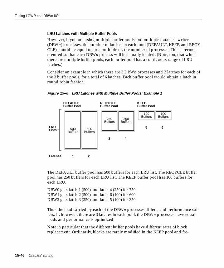
Tuning LGWR and DBWn I/O
LRU Latches with Multiple Buffer PoolsHowever, if you are using multiple buffer pools and multiple database writer(DBWn) processes, the number of latches in each pool (DEFAULT, KEEP, and RECY-CLE) should be equal to, or a multiple of, the number of processes. This is recom-mended so that each DBWn process will be equally loaded. (Note, too, that whenthere are multiple buffer pools, each buffer pool has a contiguous range of LRUlatches.)
Consider an example in which there are 3 DBWn processes and 2 latches for each ofthe 3 buffer pools, for a total of 6 latches. Each buffer pool would obtain a latch inround robin fashion.
Figure 15–6 LRU Latches with Multiple Buffer Pools: Example 1
The DEFAULT buffer pool has 500 buffers for each LRU list. The RECYCLE bufferpool has 250 buffers for each LRU list. The KEEP buffer pool has 100 buffers foreach LRU.
DBW0 gets latch 1 (500) and latch 4 (250) for 750DBW1 gets latch 2 (500) and latch 6 (100) for 600DBW2 gets latch 3 (250) and latch 5 (100) for 350
Thus the load carried by each of the DBWn processes differs, and performance suf-fers. If, however, there are 3 latches in each pool, the DBWn processes have equalloads and performance is optimized.
Note in particular that the different buffer pools have different rates of blockreplacement. Ordinarily, blocks are rarely modified in the KEEP pool and fre-
LRULists
Latches
DEFAULTBuffer Pool
RECYCLEBuffer Pool
KEEPBuffer Pool
1 2
3 4
5 6500Buffers
500Buffers
250Buffers
250Buffers
100Buffers
100Buffers
15-46 Oracle8 Tuning
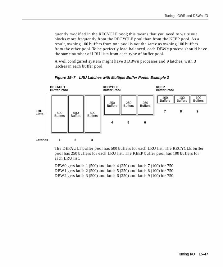
Tuning LGWR and DBWn I/O
quently modified in the RECYCLE pool; this means that you need to write outblocks more frequently from the RECYCLE pool than from the KEEP pool. As aresult, owning 100 buffers from one pool is not the same as owning 100 buffersfrom the other pool. To be perfectly load balanced, each DBWn process should havethe same number of LRU lists from each type of buffer pool.
A well configured system might have 3 DBWn processes and 9 latches, with 3latches in each buffer pool
Figure 15–7 LRU Latches with Multiple Buffer Pools: Example 2
The DEFAULT buffer pool has 500 buffers for each LRU list. The RECYCLE bufferpool has 250 buffers for each LRU list. The KEEP buffer pool has 100 buffers foreach LRU list.
DBW0 gets latch 1 (500) and latch 4 (250) and latch 7 (100) for 750DBW1 gets latch 2 (500) and latch 5 (250) and latch 8 (100) for 750DBW2 gets latch 3 (500) and latch 6 (250) and latch 9 (100) for 750
LRULists
Latches
DEFAULTBuffer Pool
RECYCLEBuffer Pool
KEEPBuffer Pool
1 2
4 5
7 8500Buffers
500Buffers
3
500Buffers
250Buffers
250Buffers
6
250Buffers
100Buffers
100Buffers
9
100Buffers
Tuning I/O 15-47

Configuring the Large Pool
Configuring the Large PoolYou can optionally configure the large pool so that Oracle has a separate pool fromwhich it can request large memory allocations. This prevents competition withother subsystems for the same memory. As Oracle allocates more shared pool mem-ory for the multithreaded server (MTS) session memory, the amount of shared poolmemory available for the shared SQL cache decreases. If you allocate session mem-ory from another area of shared memory, Oracle can use the shared pool primarilyfor caching shared SQL and not incur the performance overhead from shrinkingthe shared SQL cache.
For I/O server processes and backup and restore operations, Oracle allocates buff-ers that are a few hundred kilobytes in size. Although the shared pool may beunable to satisfy this request, the large pool will be able to do so. Note that thelarge pool does not have an LRU list; Oracle will not attempt to age memory out ofthe large pool.
Use the following parameters to configure the large pool:
■ LARGE_POOL_MIN_ALLOC
■ LARGE_POOL_SIZE
To see in which pool (shared pool or large pool) the memory for an object resides,see the column POOL in V$SGASTAT.
See Also: Oracle8 Concepts for further information about the large pool.
Oracle8 Reference for complete information about initialization parameters.
15-48 Oracle8 Tuning

Tuning Net
16
Tuning NetworksThis chapter introduces networking issues that affect tuning. Topics in this chapterinclude
■ How to Detect Network Problems
■ How to Solve Network Problems
works 16-1
How to Detect Network Problems
How to Detect Network ProblemsNetworks entail overhead that adds a certain amount of delay to processing. Tooptimize performance, you must ensure that your network throughput is fast, andthat you reduce the number of messages that must be sent over the network.
Measuring the amount of delay the network adds to performance can be difficult.Three dynamic performance views are useful in this regard: V$SESSION_EVENT,V$SESSION_WAIT, and V$SESSTAT.
In V$SESSION_EVENT, the AVERAGE_WAIT column indicates the amount of timethat Oracle waits between messages. You can use this statistic as a yardstick to eval-uate the effectiveness of the network.
In V$SESSION_WAIT, the EVENT column lists the events for which active sessionsare waiting. The “sqlnet message from client” wait event indicates that the sharedor foreground process is waiting for a message from a client. If this wait event hasoccurred, you can check to see whether the message has been sent by the user orreceived by Oracle.
You can investigate hangups by looking at V$SESSION_WAIT to see what the ses-sions are waiting for. If a client has sent a message, you can determine whether Ora-cle is responding to it or is still waiting for it.
In V$SESSTAT you can see the number of bytes that have been received from theclient, the number of bytes sent to the client, and the number of calls the client hasmade.
How to Solve Network ProblemsThis section describes several techniques for enhancing performance and solvingnetwork problems.
■ Using Array Interfaces
■ Using Prestarted Processes
■ Adjusting Session Data Unit Buffer Size
■ Increasing the Listener Queue Size
■ Using TCP.NODELAY
■ Using Shared Server Processes Rather than Dedicated Server Processes
■ Using Connection Manager
See Also: The Oracle Net8 Administrator’s Guide
16-2 Oracle8 Tuning
How to Solve Network Problems
Using Array InterfacesReduce network calls by using array interfaces. Instead of fetching one row at atime, it is more efficient to fetch ten rows with a single network round trip.
See Also: Pro*C/C++ Precompiler Programmer’s Guide and Pro*COBOL PrecompilerProgrammer’s Guide for more information on array interfaces.
Using Prestarted ProcessesPrestarting processes can improve connect time with a dedicated server. This is par-ticularly true of heavily loaded systems not using multithreaded servers, whereconnect time is slow. If prestarted processes are enabled, the listener can hand offthe connection to an existing process with no wait time whenever a connectionrequest arrives. Connection requests do not have to wait for new processes to bestarted.
Adjusting Session Data Unit Buffer SizeBefore sending data across the network, Net8 buffers data into the session data unit(SDU). It sends the data stored in this buffer when the buffer is full or when anapplication tries to read the data. When large amounts of data are being retrievedand when packet size is consistently the same, it may speed retrieval to adjust thedefault SDU size.
Optimal SDU size depends on the normal packet size. Use a sniffer to find out theframe size, or set tracing on to its highest level to check the number of packets sentand received, and to see if they are fragmented. Tune your system to limit theamount of fragmentation.
Use Oracle Network Manager to configure a change to the default SDU size onboth the client and the server; SDU size should generally be the same on both.
See Also: Oracle Net8 Administrator’s Guide
Increasing the Listener Queue SizeThe network listener active on the database server monitors and responds to con-nection requests. You can increase the listening queue for a listening process inorder to handle larger numbers of concurrent requests dynamically.
Tuning Networks 16-3
How to Solve Network Problems
Using TCP.NODELAYWhen a session is established, Net8 packages and sends data between server andclient using packets. Use the TCP.NODELAY option, which causes packets to beflushed on to the network more frequently. If you are streaming large amounts ofdata, there is no buffering and hence no delay.
Although Net8 supports many networking protocols, TCP tends to have the bestscalability.
See Also: Your platform-specific Oracle documentation
Using Shared Server Processes Rather than Dedicated Server ProcessesShared server processes, such as multithreaded server dispatchers, tend to providebetter performance than dedicated server processes. Dedicated server processes arecommitted to one session only, and exist for the duration of that session. In con-trast, a shared server process enables many clients to connect to the same serverwithout the need for a dedicated server process for each client. A dispatcher han-dles multiple incoming session requests to the shared server.
Using Connection ManagerIn Net8 you can use the Connection Manager to conserve system resources by mul-tiplexing: funneling many client sessions through a single transport connection to aserver destination. In this way you can increase the number of sessions that a pro-cess can handle.
Connection Manager you control client access to dedicated servers. In addition, itprovides multiple protocol support so that a client and server with different net-working protocols can communicate with each other.
See Also: Oracle Net8 Administrator’s Guide
16-4 Oracle8 Tuning
Tuning the Operating Sy
17
Tuning the Operating SystemThis chapter explains how to tune the operating system for optimal performance ofthe Oracle Server. Topics include:
■ Understanding Operating System Performance Issues
■ How to Detect Operating System Problems
■ How to Solve Operating System Problems
stem 17-1
Understanding Operating System Performance Issues
Understanding Operating System Performance Issues■ Overview
■ Operating System and Hardware Caches
■ Raw Devices
■ Process Schedulers
OverviewOperating system performance issues commonly involve process management,memory management, and scheduling. If you have tuned the Oracle instance per-formance and still need faster performance, you should verify your work or try toreduce system time. Make sure there is enough I/O bandwidth, CPU power, andswap space. Do not expect, however, that further tuning of the operating systemwill have a big effect on application performance. Sometimes there is simply not alot of room for improvement on the operating system side. Changes in the Oracleconfiguration or in the application itself are likely to make a bigger difference inoperating system efficiency than changing the O/S directly.
For example, if your application gives rise to a lot of buffer busy waits, the numberof system calls will increase. If you reduce the buffer busy waits by tuning theapplication, then the number of system calls will go down. Similarly, if you turn onthe Oracle initialization parameter TIMED_STATISTICS, then the number of sys-tem calls will increase; if you turn it off, then system calls will decrease.
See Also: For detailed information, see your Oracle platform-specific documenta-tion and your operating system vendor’s documentation.
Operating System and Hardware CachesOperating systems and device controllers provide data caches which do notdirectly conflict with Oracle’s own cache management, but which can consumeresources with no benefit to the user. This occurrence is most marked on a UNIXsystem with the database container files held in the UNIX file store: by default alldatabase I/O will go through the file system cache. On some UNIX-based systems,direct I/O is available to the filestore. This arrangement allows the database con-tainer files to be accessed within the UNIX file system, bypassing the file systemcache. It saves CPU resource and allows the file system cache to be dedicated tonondatabase activity such as program texts and spool files.
On NT this problem does not arise. All file requests by the database bypass thecaches in the file system.
17-2 Oracle8 Tuning
Understanding Operating System Performance Issues
Raw DevicesEvaluate the use of raw devices on your system. They involve a lot of work on thepart of the DBA, but may provide some performance benefit.
Raw devices impose a penalty on full table scans, but may be essential on UNIX-based systems if the UNIX implementation does not support write through cache.The UNIX file system speeds up full table scans by reading ahead when the serverstarts requesting contiguous data blocks. It also caches full table scans. If yourUNIX-based system does not support the write-through option on writes to the filesystem, then it is essential to use raw devices to ensure that at commit and check-point, the data which the server assumes is safely established on disk has actuallygotten there. If this is not the case, then recovery from a UNIX or system crash maynot be possible.
Raw devices on NT are similar to UNIX raw devices; however, all NT devices sup-port write through cache.
Process SchedulersMany processes (“threads” on NT systems) are involved in the operation of Oracle,and they all access the shared memory resources in the SGA.
Be sure that all Oracle processes, both background processes and user processes,have the same process priority. When you install Oracle, all background processesare given the default priority for your operating system. Do not change the priori-ties of background processes. Verify that all user processes have the default operat-ing system priority.
Assigning different priorities to Oracle processes may exacerbate the effects of con-tention. Your operating system may not grant processing time to a low-priority pro-cess if a high-priority process also requests processing time. If a high-priorityprocess needs access to a memory resource held by a low-priority process, the high-priority process may wait indefinitely for the low-priority process to obtain theCPU, process, and release the resource.
Tuning the Operating System 17-3
How to Detect Operating System Problems
How to Detect Operating System ProblemsThe key statistics to extract from any operating system monitor are
■ CPU load
■ device queues
■ network activity (queues)
■ memory management (paging/swapping)
Look at CPU utilization to see the ratio between time spent running in applicationmode and time spent running in operating system mode. Look at run queues to seehow many processes are runable and how many system calls are being executed.See if paging or swapping is occurring, and check the number of I/Os being per-formed.
See Also: Your Oracle platform-specific documentation and your operating systemvendor’s documentation.
17-4 Oracle8 Tuning
How to Solve Operating System Problems
How to Solve Operating System ProblemsThis section provides hints for tuning various systems.
■ Performance on UNIX-Based Systems
■ Performance on NT Systems
■ Performance on Mainframe Computers
Familiarize yourself with platform-specific issues, so that you know what perfor-mance options your operating system provides. For example, some platforms havepost wait drivers, which allow you to map system time and thus reduce systemcalls, enabling faster I/O.
See Also: Your Oracle platform-specific documentation and your operating systemvendor’s documentation.
Performance on UNIX-Based SystemsOn UNIX-based systems, try to find a good ratio between the amount of time theoperating system runs (fulfilling system calls and doing process scheduling), andthe amount of time the application runs. Your goal should be running 60% to 75%of the time in application mode, and 25% to 40% of the time in operating systemmode. If you find that the system is spending 50% of its time in each mode, thenyou should investigate to determine what is wrong.
The ratio of time spent in each mode is only a symptom of the underlying problem,which might have to do with:
■ swapping
■ executing too many O/S system calls
■ running too many processes
If such conditions exist, then there is less time available for the application to run.The more time you can release from the operating system side, the more transac-tions your application can perform.
Tuning the Operating System 17-5
How to Solve Operating System Problems
Performance on NT SystemsOn NT systems, as with UNIX-based systems, you should establish an appropriateratio between time in application mode and time in system mode. On NT you caneasily monitor many factors with Performance Monitor: CPU, network, I/O, andmemory are all displayed on the same graph, to assist you in avoiding bottlenecksin any of these areas. Note that the term “process” as used in this tuning manualrefers to a “thread” in the NT environment.
Performance on Mainframe ComputersConsider the paging parameters on a mainframe, and remember that Oracle canexploit a very large working set.
Free memory in a VAX/VMS environment is actually memory that is not currentlymapped to any operating system process. On a busy system, free memory is likelyto contain a page that belongs to one or more currently active process. When thataccess occurs a “soft page fault” takes place, and the page is included in the work-ing set for the process. If the process cannot expand its working set, then one of thepages currently mapped by the process must be moved to the free set.
Any number of processes may have pages of shared memory within their workingsets. The sum of the sizes of the working sets can thus markedly exceed the avail-able memory. When Oracle Server is running, the SGA, the Oracle kernel code, andthe Oracle Forms runtime executable are normally all sharable and account for per-haps 80% or 90% of the pages accessed.
Adding more buffers is not necessarily better. Each application has a thresholdnumber of buffers at which the cache hit ratio stops rising. This is typically quitelow (approximately 1500 buffers). Setting higher values simply increases the man-agement load for both Oracle and the operating system.
17-6 Oracle8 Tuning
Tuning Resource Conte
18
Tuning Resource ContentionContention occurs when multiple processes try to access the same resource simulta-neously. Some processes must then wait for access to various database structures.Topics discussed in this chapter include:
■ Understanding Contention Issues
■ How to Detect Contention Problems
■ How to Solve Contention Problems
■ Reducing Contention for Rollback Segments
■ Reducing Contention for Multithreaded Server Processes
■ Reducing Contention for Parallel Server Processes
■ Reducing Contention for Redo Log Buffer Latches
■ Reducing Contention for the LRU Latch
■ Reducing Free List Contention
ntion 18-1
Understanding Contention Issues
Understanding Contention IssuesSymptoms of resource contention problems can be found in V$SYSTEM_EVENT.This view reveals various system problems that may be impacting performance,problems such as latch contention, buffer contention, I/O contention. It is impor-tant to remember that these are only symptoms of problems—not the actual causes.
For example, by looking at V$SYSTEM_EVENT you might notice lots of buffer-busy waits. It may be that many processes are inserting into the same block andmust wait for each other before they can insert. The solution might be to introducefree lists for the object in question.
Buffer busy waits may also have caused some latch free waits. Since most of thesewaits were caused by misses on the cache buffer hash chain latch, this was also aside effect of trying to insert into the same block. Rather than increasing SPIN-COUNT to reduce the latch free waits (a symptom), you should change the objectto allow for multiple processes to insert into free blocks. This approach will effec-tively reduce contention.
See Also: Oracle8 Administrator’s Guide to understand which resources are used byvarious Oracle8 features.
18-2 Oracle8 Tuning
How to Solve Contention Problems
How to Detect Contention ProblemsThe V$RESOURCE_LIMIT view provides information about current and maximumglobal resource utilization for some system resources. This information enables youto make better decisions when choosing values for resource limit-controllingparameters.
If the system has idle time, start your investigation by checkingV$SYSTEM_EVENT. Examine the events with the highest average wait time, thentake appropriate action on each. For example, if you find a high number of latchfree waits, look in V$LATCH to see which latch is the problem.
For excessive buffer busy waits, look in V$WAITSTAT to see which block type hasthe highest wait count and the highest wait time. Look in V$SESSION_WAIT forcache buffer waits so you can decode the file and block number of an object.
The rest of this chapter describes common contention problems. Remember that thedifferent forms of contention are symptoms which can be fixed by making changesin one of two places:
■ changes in the application
■ changes in Oracle
Sometimes you have no alternative but to change the application in order to over-come performance constraints.
How to Solve Contention ProblemsThe rest of this chapter examines various kinds of contention and explains how toresolve problems. Contention may be for rollback segments, multithreaded serverprocesses, parallel server processes, redo log buffer latches, LRU latch, or for freelists.
Tuning Resource Contention 18-3
Reducing Contention for Rollback Segments
Reducing Contention for Rollback SegmentsIn this section, you will learn how to reduce contention for rollback segments. Thefollowing issues are discussed:
■ Identifying Rollback Segment Contention
■ Creating Rollback Segments
Identifying Rollback Segment ContentionContention for rollback segments is reflected by contention for buffers that containrollback segment blocks. You can determine whether contention for rollback seg-ments is reducing performance by checking the dynamic performance tableV$WAITSTAT.
V$WAITSTAT contains statistics that reflect block contention. By default, this tableis available only to the user SYS and to other users who have SELECT ANY TABLEsystem privilege, such as SYSTEM. These statistics reflect contention for differentclasses of block:
Use the following query to monitor these statistics over a period of time while yourapplication is running:
SELECT class, count FROM v$waitstat WHERE class IN (’system undo header’, ’system undo block’, ’undo header’, ’undo block’);
SYSTEM UNDO HEADER the number of waits for buffers containingheader blocks of the SYSTEM rollback segment
SYSTEM UNDO BLOCK the number of waits for buffers containingblocks of the SYSTEM rollback segment otherthan header blocks
UNDO HEADER the number of waits for buffers containingheader blocks of rollback segments other thanthe SYSTEM rollback segment
UNDO BLOCK the number of waits for buffers containingblocks other than header blocks of rollback seg-ments other than the SYSTEM rollback segment
18-4 Oracle8 Tuning
Reducing Contention for Rollback Segments
The result of this query might look like this:
CLASS COUNT------------------ ----------system undo header 2089system undo block 633undo header 1235undo block 942
Compare the number of waits for each class of block with the total number ofrequests for data over the same period of time. You can monitor the total number ofrequests for data over a period of time with this query:
SELECT SUM(value) FROM v$sysstat WHERE name IN (’db block gets’, ’consistent gets’);
The output of this query might look like this:
SUM(VALUE)---------- 929530
The information in V$SYSSTAT can also be obtained through SNMP.
If the number of waits for any class is greater than 1% of the total number ofrequests, consider creating more rollback segments to reduce contention.
Creating Rollback SegmentsTo reduce contention for buffers containing rollback segment blocks, create morerollback segments. Table 18–1 shows some general guidelines for choosing howmany rollback segments to allocate based on the number of concurrent transactionson your database. These guidelines are appropriate for most application mixes.
Table 18–1 Choosing the Number of Rollback Segments
Number of Current Transactions ( n)Number of Rollback SegmentsRecommended
n < 16 4
16 <= n < 32 8
32 <= n n/4
Tuning Resource Contention 18-5
Reducing Contention for Multithreaded Server Processes
Reducing Contention for Multithreaded Server ProcessesIn this section, you will learn how to reduce contention for some of the processesused by the Oracle’s multithreaded server architecture:
■ Reducing Contention for Dispatcher Processes
■ Reducing Contention for Shared Server Processes
Reducing Contention for Dispatcher ProcessesThis section discusses how to identify contention for dispatcher processes, how toadd dispatcher processes, and how to enable connection pooling.
Identifying Contention for Dispatcher ProcessesContention for dispatcher processes can be reflected by either of these symptoms:
■ high busy rates for existing dispatcher processes
■ steady increase in waiting time for responses in the response queues of existingdispatcher processes
Examining Busy Rates for Dispatcher Processes V$DISPATCHER contains statisticsreflecting the activity of dispatcher processes. By default, this table is available onlyto the user SYS and to other users who have SELECT ANY TABLE system privi-lege, such as SYSTEM. These columns reflect busy rates for dispatcher processes:
Use the following query to monitor these statistics over a period of time while yourapplication is running:
SELECT network "Protocol", SUM(busy) / ( SUM(busy) + SUM(idle) ) "Total Busy Rate" FROM v$dispatcher GROUP BY network;
This query returns the total busy rate for the dispatcher processes of each protocol;that is, the percentage of time the dispatcher processes of each protocol are busy.The result of this query might look like this:
IDLE the idle time for the dispatcher process in hundredths of asecond
BUSY the busy time for the dispatcher process in hundredths of asecond
18-6 Oracle8 Tuning
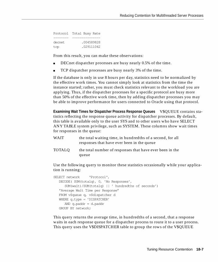
Reducing Contention for Multithreaded Server Processes
Protocol Total Busy Rate-------- ---------------decnet .004589828tcp .029111042
From this result, you can make these observations:
■ DECnet dispatcher processes are busy nearly 0.5% of the time.
■ TCP dispatcher processes are busy nearly 3% of the time.
If the database is only in use 8 hours per day, statistics need to be normalized bythe effective work times. You cannot simply look at statistics from the time theinstance started; rather, you must check statistics relevant to the workload you areapplying. Thus, if the dispatcher processes for a specific protocol are busy morethan 50% of the effective work time, then by adding dispatcher processes you maybe able to improve performance for users connected to Oracle using that protocol.
Examining Wait Times for Dispatcher Process Response Queues V$QUEUE contains sta-tistics reflecting the response queue activity for dispatcher processes. By default,this table is available only to the user SYS and to other users who have SELECTANY TABLE system privilege, such as SYSTEM. These columns show wait timesfor responses in the queue:
Use the following query to monitor these statistics occasionally while your applica-tion is running:
SELECT network "Protocol", DECODE( SUM(totalq), 0, ’No Responses’, SUM(wait)/SUM(totalq) || ’ hundredths of seconds’) ”Average Wait Time per Response” FROM v$queue q, v$dispatcher d WHERE q.type = ’DISPATCHER’ AND q.paddr = d.paddr GROUP BY network;
This query returns the average time, in hundredths of a second, that a responsewaits in each response queue for a dispatcher process to route it to a user process.This query uses the V$DISPATCHER table to group the rows of the V$QUEUE
WAIT the total waiting time, in hundredths of a second, for allresponses that have ever been in the queue
TOTALQ the total number of responses that have ever been in thequeue
Tuning Resource Contention 18-7
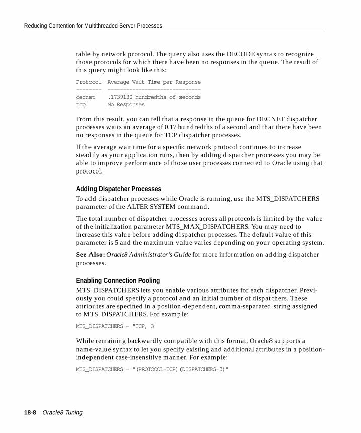
Reducing Contention for Multithreaded Server Processes
table by network protocol. The query also uses the DECODE syntax to recognizethose protocols for which there have been no responses in the queue. The result ofthis query might look like this:
Protocol Average Wait Time per Response-------- ------------------------------decnet .1739130 hundredths of secondstcp No Responses
From this result, you can tell that a response in the queue for DECNET dispatcherprocesses waits an average of 0.17 hundredths of a second and that there have beenno responses in the queue for TCP dispatcher processes.
If the average wait time for a specific network protocol continues to increasesteadily as your application runs, then by adding dispatcher processes you may beable to improve performance of those user processes connected to Oracle using thatprotocol.
Adding Dispatcher ProcessesTo add dispatcher processes while Oracle is running, use the MTS_DISPATCHERSparameter of the ALTER SYSTEM command.
The total number of dispatcher processes across all protocols is limited by the valueof the initialization parameter MTS_MAX_DISPATCHERS. You may need toincrease this value before adding dispatcher processes. The default value of thisparameter is 5 and the maximum value varies depending on your operating system.
See Also: Oracle8 Administrator’s Guide for more information on adding dispatcherprocesses.
Enabling Connection PoolingMTS_DISPATCHERS lets you enable various attributes for each dispatcher. Previ-ously you could specify a protocol and an initial number of dispatchers. Theseattributes are specified in a position-dependent, comma-separated string assignedto MTS_DISPATCHERS. For example:
MTS_DISPATCHERS = "TCP, 3"
While remaining backwardly compatible with this format, Oracle8 supports aname-value syntax to let you specify existing and additional attributes in a position-independent case-insensitive manner. For example:
MTS_DISPATCHERS = "(PROTOCOL=TCP)(DISPATCHERS=3)"
18-8 Oracle8 Tuning
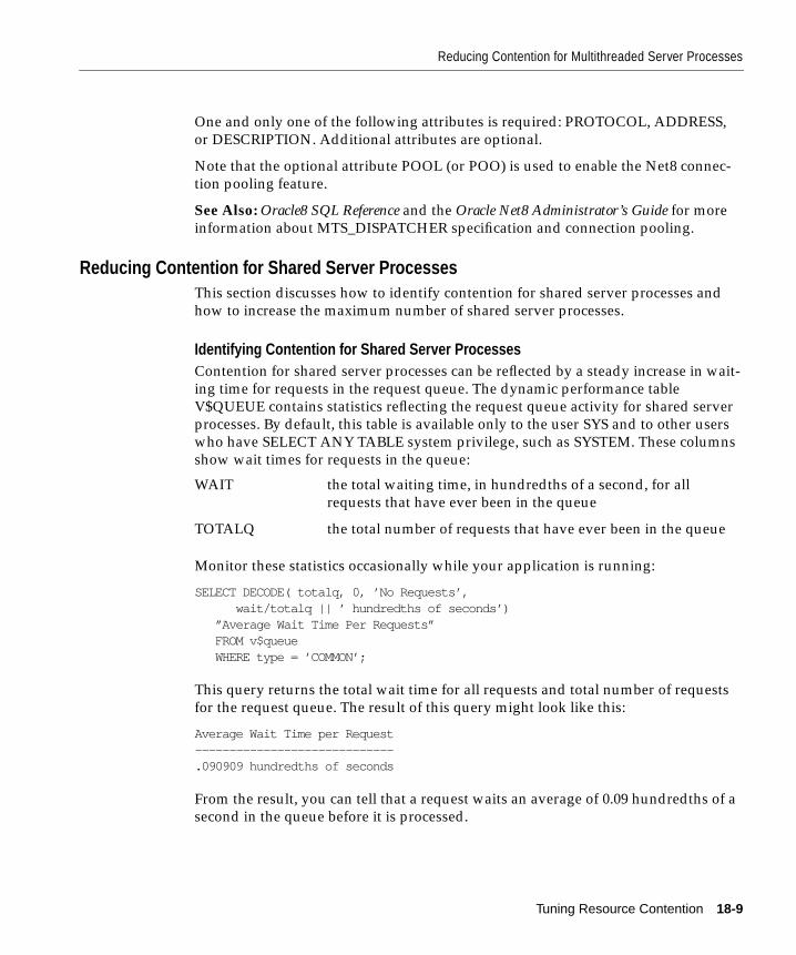
Reducing Contention for Multithreaded Server Processes
One and only one of the following attributes is required: PROTOCOL, ADDRESS,or DESCRIPTION. Additional attributes are optional.
Note that the optional attribute POOL (or POO) is used to enable the Net8 connec-tion pooling feature.
See Also: Oracle8 SQL Reference and the Oracle Net8 Administrator’s Guide for moreinformation about MTS_DISPATCHER specification and connection pooling.
Reducing Contention for Shared Server ProcessesThis section discusses how to identify contention for shared server processes andhow to increase the maximum number of shared server processes.
Identifying Contention for Shared Server ProcessesContention for shared server processes can be reflected by a steady increase in wait-ing time for requests in the request queue. The dynamic performance tableV$QUEUE contains statistics reflecting the request queue activity for shared serverprocesses. By default, this table is available only to the user SYS and to other userswho have SELECT ANY TABLE system privilege, such as SYSTEM. These columnsshow wait times for requests in the queue:
Monitor these statistics occasionally while your application is running:
SELECT DECODE( totalq, 0, ’No Requests’, wait/totalq || ’ hundredths of seconds’) ”Average Wait Time Per Requests” FROM v$queue WHERE type = ’COMMON’;
This query returns the total wait time for all requests and total number of requestsfor the request queue. The result of this query might look like this:
Average Wait Time per Request-----------------------------.090909 hundredths of seconds
From the result, you can tell that a request waits an average of 0.09 hundredths of asecond in the queue before it is processed.
WAIT the total waiting time, in hundredths of a second, for allrequests that have ever been in the queue
TOTALQ the total number of requests that have ever been in the queue
Tuning Resource Contention 18-9
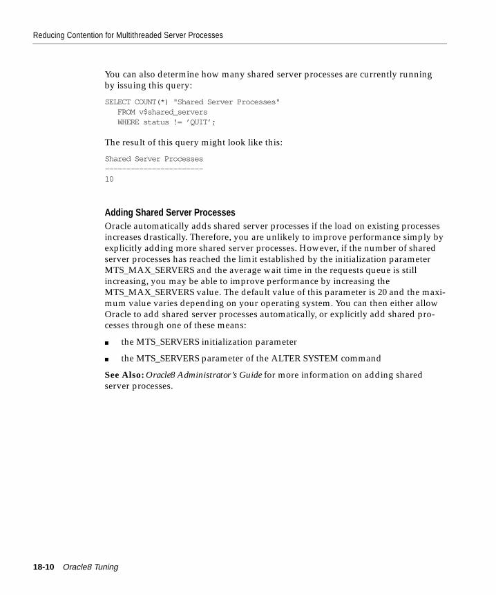
Reducing Contention for Multithreaded Server Processes
You can also determine how many shared server processes are currently runningby issuing this query:
SELECT COUNT(*) "Shared Server Processes" FROM v$shared_servers WHERE status != ’QUIT’;
The result of this query might look like this:
Shared Server Processes-----------------------10
Adding Shared Server ProcessesOracle automatically adds shared server processes if the load on existing processesincreases drastically. Therefore, you are unlikely to improve performance simply byexplicitly adding more shared server processes. However, if the number of sharedserver processes has reached the limit established by the initialization parameterMTS_MAX_SERVERS and the average wait time in the requests queue is stillincreasing, you may be able to improve performance by increasing theMTS_MAX_SERVERS value. The default value of this parameter is 20 and the maxi-mum value varies depending on your operating system. You can then either allowOracle to add shared server processes automatically, or explicitly add shared pro-cesses through one of these means:
■ the MTS_SERVERS initialization parameter
■ the MTS_SERVERS parameter of the ALTER SYSTEM command
See Also: Oracle8 Administrator’s Guide for more information on adding sharedserver processes.
18-10 Oracle8 Tuning
Reducing Contention for Parallel Server Processes
Reducing Contention for Parallel Server ProcessesThis section describes how to detect and alleviate contention for parallel server pro-cesses when using parallel execution:
■ Identifying Contention for Parallel Server Processes
■ Reducing Contention for Parallel Server Processes
Identifying Contention for Parallel Server ProcessesStatistics in the V$PQ_SYSSTAT view are useful for determining the appropriatenumber of parallel server processes for an instance. The statistics that are particu-larly useful are SERVERS BUSY, SERVERS IDLE, SERVERS STARTED, and SERV-ERS SHUTDOWN.
Frequently, you will not be able to increase the maximum number of parallel serverprocesses for an instance because the maximum number is heavily dependent uponthe capacity of your CPUs and your I/O bandwidth. However, if servers are contin-uously starting and shutting down, you should consider increasing the value of theparameter PARALLEL_MIN_SERVERS.
For example, if you have determined that the maximum number of concurrent par-allel server processes that your machine can manage is 100, you should setPARALLEL_MAX_SERVERS to 100. Next, determine how many parallel server pro-cesses the average parallel operation needs, and how many parallel operations arelikely to be executed concurrently. For this example, assume you will have two con-current operations with 20 as the average degree of parallelism. Thus at any giventime there could be 80 parallel server processes busy on an instance. Thus youshould set the PARALLEL_MIN_SERVERS parameter to 80.
Periodically examine V$PQ_SYSSTAT to determine whether the 80 parallel serverprocesses for the instance are actually busy. To do so, issue the following query:
SELECT * FROM V$PQ_SYSSTATWHERE statistic = "Servers Busy";
The result of this query might look like this:
STATISTIC VALUE--------------------- -----------Servers Busy 70
Tuning Resource Contention 18-11
Reducing Contention for Redo Log Buffer Latches
Reducing Contention for Parallel Server ProcessesIf you find that typically there are fewer than PARALLEL_MIN_SERVERS busy atany given time, your idle parallel server processes constitute system overhead thatis not being used. Consider decreasing the value of the parameterPARALLEL_MIN_SERVERS. If you find that there are typically more parallelserver processes active than the value of PARALLEL_MIN_SERVERS and the SERV-ERS STARTED statistic is continuously growing, consider increasing the value ofthe parameter PARALLEL_MIN_SERVERS.
Reducing Contention for Redo Log Buffer LatchesContention for redo log buffer access rarely inhibits database performance. How-ever, Oracle provides methods to monitor and reduce any latch contention thatdoes occur. This section covers:
■ Detecting Contention for Space in the Redo Log Buffer
■ Detecting Contention for Redo Log Buffer Latches
■ Examining Redo Log Activity
■ Reducing Latch Contention
Detecting Contention for Space in the Redo Log BufferWhen LGWR writes redo entries from the redo log buffer to a redo log file, user pro-cesses can then copy new entries over the entries that have been written to disk.LGWR normally writes fast enough to ensure that space is always available in thebuffer for new entries, even when access to the redo log is heavy.
The statistic REDO BUFFER ALLOCATION RETRIES reflects the number of timesa user process waits for space in the redo log buffer. This statistic is availablethrough the dynamic performance table V$SYSSTAT. By default, this table is avail-able only to the user SYS and to users granted SELECT ANY TABLE system privi-lege, such as SYSTEM. Use the following query to monitor these statistics over aperiod of time while your application is running:
SELECT name, value FROM v$sysstat WHERE name = ’redo buffer allocation retries’;
The information in V$SYSSTAT can also be obtained through the Simple NetworkManagement Protocol (SNMP).
18-12 Oracle8 Tuning
Reducing Contention for Redo Log Buffer Latches
The value of REDO BUFFER ALLOCATION RETRIES should be near 0. If thisvalue increments consistently, processes have had to wait for space in the buffer.The wait may be caused by the log buffer being too small, or by checkpointing orlog switching. Increase the size of the redo log buffer, if necessary, by changing thevalue of the initialization parameter LOG_BUFFER. The value of this parameter,expressed in bytes, must be a multiple of DB_BLOCK_SIZE. Alternatively, improvethe checkpointing or archiving process.
Note: Multiple archiver processes are not recommended. A single automatic ARCHprocess can archive redo logs, keeping pace with the LGWR process.
Detecting Contention for Redo Log Buffer LatchesAccess to the redo log buffer is regulated by two types of latch: the redo allocationlatch and redo copy latches
The Redo Allocation LatchThe redo allocation latch controls the allocation of space for redo entries in the redolog buffer. To allocate space in the buffer, an Oracle user process must obtain theredo allocation latch. Since there is only one redo allocation latch, only one user pro-cess can allocate space in the buffer at a time. The single redo allocation latchenforces the sequential nature of the entries in the buffer.
After allocating space for a redo entry, the user process may copy the entry into thebuffer. This is called “copying on the redo allocation latch”. A process may onlycopy on the redo allocation latch if the redo entry is smaller than a threshold size.
The maximum size of a redo entry that can be copied on the redo allocation latch isspecified by the initialization parameter LOG_SMALL_ENTRY_MAX_SIZE. Thevalue of this parameter is expressed in bytes. The minimum, maximum, anddefault values vary depending on your operating system.
Redo Copy LatchesThe user process first obtains the copy latch. Then it obtains the allocation latch,performs allocation, and releases the allocation latch. Next the process performs thecopy under the copy latch, and releases the copy latch. The allocation latch is thusheld for only a very short period of time, as the user process does not try to obtainthe copy latch while holding the allocation latch.
If the redo entry is too large to copy on the redo allocation latch, the user processmust obtain a redo copy latch before copying the entry into the buffer. While hold-ing a redo copy latch, the user process copies the redo entry into its allocated spacein the buffer and then releases the redo copy latch.
Tuning Resource Contention 18-13
Reducing Contention for Redo Log Buffer Latches
If your computer has multiple CPUs, your redo log buffer can have multiple redocopy latches. These allow multiple processes to copy entries to the redo log bufferconcurrently. The number of redo copy latches is determined by the parameterLOG_SIMULTANEOUS_COPIES; its default value is the number of CPUs availableto your Oracle instance.
On single-CPU computers, there should be no redo copy latches, because only oneprocess can by active at once. In this case, all redo entries are copied on the redoallocation latch, regardless of size.
Examining Redo Log ActivityHeavy access to the redo log buffer can result in contention for redo log bufferlatches. Latch contention can reduce performance. Oracle collects statistics for theactivity of all latches and stores them in the dynamic performance table V$LATCH.By default, this table is available only to the user SYS and to other users who haveSELECT ANY TABLE system privilege, such as SYSTEM.
Each row in the V$LATCH table contains statistics for a different type of latch. Thecolumns of the table reflect activity for different types of latch requests. The distinc-tion between these types of requests is whether the requesting process continues torequest a latch if it is unavailable:
These columns of the V$LATCH table reflect willing-to-wait requests:
For example, consider the case in which a process makes a willing-to-wait requestfor a latch that is unavailable. The process waits and requests the latch again and
WILLING-TO-WAIT
If the latch requested with a willing-to-wait request is notavailable, the requesting process waits a short time andrequests the latch again. The process continues waiting andrequesting until the latch is available.
IMMEDIATE If the latch requested with an immediate request is not avail-able, the requesting process does not wait, but continues pro-cessing.
GETS shows the number of successful willing-to-wait requests fora latch
MISSES shows the number of times an initial willing-to-wait requestwas unsuccessful
SLEEPS shows the number of times a process waited and requested alatch after an initial willing-to-wait request
18-14 Oracle8 Tuning
Reducing Contention for Redo Log Buffer Latches
the latch is still unavailable. The process waits and requests the latch a third timeand acquires the latch. This activity increments the statistics as follows:
■ The GETS value increases by one, since one request for the latch (the thirdrequest) was successful.
■ The MISSES value increases by one, since the initial request for the latchresulted in waiting.
■ The SLEEPS value increases by two, since the process waited for the latchtwice, once after the initial request and again after the second request.
These columns of the V$LATCH table reflect immediate requests:
Use the following query to monitor the statistics for the redo allocation latch andthe redo copy latches over a period of time:
SELECT ln.name, gets, misses, immediate_gets, immediate_misses FROM v$latch l, v$latchname ln WHERE ln.name IN (’redo allocation’, ’redo copy’) AND ln.latch# = l.latch#;
The output of this query might look like this:
NAME GETS MISSES IMMEDIATE_GETS IMMEDIATE_MISSES------------ ---------- ---------- -------------- ----------------redo allo... 252867 83 0 0redo copy 0 0 22830 0
From the output of the query, calculate the wait ratio for each type of request.
Contention for a latch may affect performance if either of these conditions is true:
■ if the ratio of MISSES to GETS exceeds 1%
■ if the ratio of IMMEDIATE_MISSES to the sum of IMMEDIATE_GETS andIMMEDIATE_MISSES exceeds 1%
If either of these conditions is true for a latch, try to reduce contention for thatlatch. These contention thresholds are appropriate for most operating systems,though some computers with many CPUs may be able to tolerate more contentionwithout performance reduction.
IMMEDIATE GETS This column shows the number of successful imme-diate requests for each latch.
IMMEDIATE MISSES This column shows the number of unsuccessfulimmediate requests for each latch.
Tuning Resource Contention 18-15
Reducing Contention for the LRU Latch
Reducing Latch ContentionMost cases of latch contention occur when two or more Oracle processes concur-rently attempt to obtain the same latch. Latch contention rarely occurs on single-CPU computers, where only a single process can be active at once.
Reducing Contention for the Redo Allocation LatchTo reduce contention for the redo allocation latch, you should minimize the timethat any single process holds the latch. To reduce this time, reduce copying on theredo allocation latch. Decreasing the value of theLOG_SMALL_ENTRY_MAX_SIZE initialization parameter reduces the numberand size of redo entries copied on the redo allocation latch.
Reducing Contention for Redo Copy LatchesOn multiple-CPU computers, multiple redo copy latches allow multiple processesto copy entries to the redo log buffer concurrently. The default value ofLOG_SIMULTANEOUS_COPIES is the number of CPUs available to your Oracleinstance.
If you observe contention for redo copy latches, add more latches by increasing thevalue of LOG_SIMULTANEOUS_COPIES. It can help to have up to twice as manyredo copy latches as CPUs available to your Oracle instance.
Reducing Contention for the LRU LatchThe LRU (least recently used) latch controls the replacement of buffers in the buffercache. For symmetric multiprocessor (SMP) systems, Oracle automatically sets thenumber of LRU latches to be one half the number of CPUs on the system. For non-SMP systems, one LRU latch is sufficient.
Contention for the LRU latch can impede performance on SMP machines with alarge number of CPUs. You can detect LRU latch contention by queryingV$LATCH, V$SESSION_EVENT, and V$SYSTEM_EVENT. To avoid contention,consider bypassing the buffer cache or redesigning the application.
You can specify the number of LRU latches on your system with the initializationparameter DB_BLOCK_LRU_LATCHES. This parameter sets the maximum valuefor the desired number of LRU latches. Each LRU latch controls a set of buffers;Oracle balances allocation of replacement buffers among the sets.
To select the appropriate value for DB_BLOCK_LRU_LATCHES, consider the fol-lowing:
18-16 Oracle8 Tuning
Reducing Free List Contention
■ The maximum number of latches is twice the number of CPUs in the system.That is, the value of DB_BLOCK_LRU_LATCHES can range from 1 to twice thenumber of CPUs.
■ A latch should have no less than 50 buffers in its set; for small buffer cachesthere is no added value if you select a larger number of sets. The size of thebuffer cache determines a maximum boundary condition on the number of sets.
■ Do not create multiple latches when Oracle runs in single process mode. Oracleautomatically uses only one LRU latch in single process mode.
■ If the workload on the instance is large, then you should have a higher numberof latches. For example, if you have 32 CPUs in your system, choose a numberbetween half the number of CPUs (16) and actual number of CPUs (32) in yoursystem.
Note: You cannot dynamically change the number of sets during the lifetime of theinstance.
Reducing Free List ContentionFree list contention can reduce the performance of some applications. This sectioncovers:
■ Identifying Free List Contention
■ Adding More Free Lists
Identifying Free List ContentionContention for free lists is reflected by contention for free data blocks in the buffercache. You can determine whether contention for free lists is reducing performanceby querying the dynamic performance table V$WAITSTAT.
The V$WAITSTAT table contains block contention statistics. By default, this table isavailable only to the user SYS and to other users who have SELECT ANY TABLEsystem privilege, such as SYSTEM.
Use the following procedure to find the segment names and free lists that have con-tention:
1. Check V$WAITSTAT for contention on DATA BLOCKS.
2. Check V$SYSTEM_EVENT for BUFFER BUSY WAITS.
High numbers indicate that some contention exists.
Tuning Resource Contention 18-17
Reducing Free List Contention
3. In this case, check V$SESSION_WAIT to see, for each buffer busy wait, the val-ues for FILE, BLOCK, and ID.
4. Construct a query as follows to obtain the name of the objects and free lists thathave the buffer busy waits:
SELECT SEGMENT_NAME, SEGMENT_TYPEFROM DBA_EXTENTSWHERE FILE_ID = fileAND BLOCK BETWEENblock_id AND block_id + blocks ;
This will return the segment name (segment) and type (type).
5. To find the free lists, query as follows:
SELECT SEGMENT_NAME, FREELISTSFROM DBA_SEGMENTSWHERE SEGMENT_NAME =segmentAND SEGMENT_TYPE =type ;
Adding More Free ListsTo reduce contention for the free lists of a table, re-create the table with a largervalue for the FREELISTS storage parameter. Increasing the value of this parameterto the number of Oracle processes that concurrently insert data into the table mayimprove performance of the INSERT statements.
Re-creating the table may simply involve dropping and creating it again. However,you may want to use one of these means instead:
■ Re-create the table by selecting data from the old table into a new table, drop-ping the old table, and renaming the new one.
■ Use Export and Import to export the table, drop the table, and import the table.This measure avoids consuming space by creating a temporary table.
18-18 Oracle8 Tuning
Part V
Optimizing Parallel ExecutionPart V discusses parallel execution tuning. The chapters in Part 5 are:
■ Chapter 19, “Tuning Parallel Execution”
■ Chapter 20, “Understanding Parallel Execution Performance Issues”
■ Chapter 21, “Diagnosing Parallel Execution Performance Problems”

Tuning Parallel Exec
19
Tuning Parallel ExecutionParallel execution can dramatically reduce response time for data-intensive opera-tions on very large databases. This chapter explains how to tune your system foroptimal performance of parallel operations.
■ Introduction to Parallel Execution Tuning
■ Step 1: Tuning System Parameters for Parallel Execution
■ Step 2: Tuning Physical Database Layout for Parallel Execution
■ Step 3: Analyzing Data
See Also: Oracle8 Concepts, for basic principles of parallel execution.
See your operating system-specific Oracle documentation for more informationabout tuning while using parallel execution.
ution 19-1
Introduction to Parallel Execution Tuning
Introduction to Parallel Execution TuningParallel execution is useful for operations that access a large amount of data by wayof large table scans, large joins, the creation of large indexes, partitioned indexscans; bulk inserts, updates, deletes; aggregation or copying. It benefits systemswith all of the following characteristics:
■ symmetric multiprocessors (SMP), clusters, or massively parallel systems
■ high I/O bandwidth (that is, many datafiles on many different disk drives)
■ underutilized or intermittently used CPUs (for example, systems where CPUusage is typically less than 30%)
■ sufficient memory to support additional memory-intensive processes such assorts, hashing, and I/O buffers
If any one of these conditions is not true for your system, parallel execution may notsignificantly help performance. In fact, on over-utilized systems or systems withsmall I/O bandwidth, parallel execution can impede system performance.
Note: In this chapter the term “parallel server process” designates a process (or athread, on NT systems) that is performing a parallel operation, as distinguishedfrom the product “Oracle Parallel Server”.
19-2 Oracle8 Tuning
Step 1: Tuning System Parameters for Parallel Execution
Step 1: Tuning System Parameters for Parallel ExecutionMany initialization parameters affect parallel execution performance. For bestresults, start with an initialization file that is appropriate for the intended applica-tion.
Before starting the Oracle Server, set the initialization parameters described in thissection. The recommended settings are guidelines for a large data warehouse (morethan 100 gigabytes) on a typical high-end shared memory multiprocessor with oneor two gigabytes of memory. Each section explains how to modify these settings forother configurations. Note that you can change some of these parameters dynami-cally with ALTER SYSTEM or ALTER SESSION statements. The parameters aregrouped as follows:
■ Parameters Affecting Resource Consumption for All Parallel Operations
■ Parameters Affecting Resource Consumption for Parallel DML & Parallel DDL
■ Parameters Enabling New Features
■ Parameters Related to I/O
Parameters Affecting Resource Consumption for All Parallel OperationsThe parameters discussed in this section affect the consumption of memory andother resources for all parallel operations, and in particular for parallel query.Chapter 20, “Understanding Parallel Execution Performance Issues” describes indetail how these parameters interrelate.
You must configure memory at two levels:
■ at the Oracle level, so that the system uses an appropriate amount of memoryfrom the operating system
■ at the operating system level, for consistency. On some platforms you mayneed to set operating system parameters which control the total amount of vir-tual memory available, summed across all processes.
The SGA is typically part of the real physical memory. The SGA is static, of fixedsize; if you want to change its size you must shut down the database, make thechange, and restart the database.
The memory used in data warehousing operations is much more dynamic. It comesout of process memory: and both the size of a process’ memory and the number ofprocesses can vary greatly.
Tuning Parallel Execution 19-3
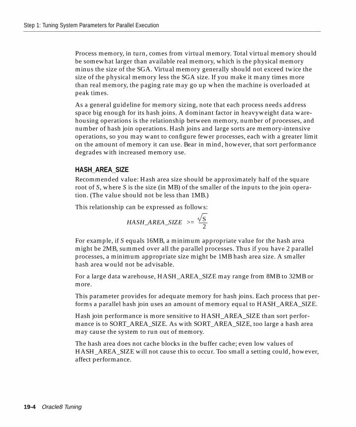
Step 1: Tuning System Parameters for Parallel Execution
Process memory, in turn, comes from virtual memory. Total virtual memory shouldbe somewhat larger than available real memory, which is the physical memoryminus the size of the SGA. Virtual memory generally should not exceed twice thesize of the physical memory less the SGA size. If you make it many times morethan real memory, the paging rate may go up when the machine is overloaded atpeak times.
As a general guideline for memory sizing, note that each process needs addressspace big enough for its hash joins. A dominant factor in heavyweight data ware-housing operations is the relationship between memory, number of processes, andnumber of hash join operations. Hash joins and large sorts are memory-intensiveoperations, so you may want to configure fewer processes, each with a greater limiton the amount of memory it can use. Bear in mind, however, that sort performancedegrades with increased memory use.
HASH_AREA_SIZERecommended value: Hash area size should be approximately half of the squareroot of S, where S is the size (in MB) of the smaller of the inputs to the join opera-tion. (The value should not be less than 1MB.)
This relationship can be expressed as follows:
For example, if S equals 16MB, a minimum appropriate value for the hash areamight be 2MB, summed over all the parallel processes. Thus if you have 2 parallelprocesses, a minimum appropriate size might be 1MB hash area size. A smallerhash area would not be advisable.
For a large data warehouse, HASH_AREA_SIZE may range from 8MB to 32MB ormore.
This parameter provides for adequate memory for hash joins. Each process that per-forms a parallel hash join uses an amount of memory equal to HASH_AREA_SIZE.
Hash join performance is more sensitive to HASH_AREA_SIZE than sort perfor-mance is to SORT_AREA_SIZE. As with SORT_AREA_SIZE, too large a hash areamay cause the system to run out of memory.
The hash area does not cache blocks in the buffer cache; even low values ofHASH_AREA_SIZE will not cause this to occur. Too small a setting could, however,affect performance.
HASH_AREA_SIZE >= S2
19-4 Oracle8 Tuning
Step 1: Tuning System Parameters for Parallel Execution
Note that HASH_AREA_SIZE is relevant to parallel query operations, and to thequery portion of DML or DDL statements.
See Also: "SORT_AREA_SIZE" on page 19-12
OPTIMIZER_PERCENT_PARALLELRecommended value: 100/number_of_concurrent_users
This parameter determines how aggressively the optimizer attempts to parallelize agiven execution plan. OPTIMIZER_PERCENT_PARALLEL encourages the opti-mizer to use plans that have low response time because of parallel execution, evenif total resource used is not minimized.
The default value of OPTIMIZER_PERCENT_PARALLEL is 0, which parallelizesthe plan that uses the least resource, if possible. Here, the execution time of theoperation may be long because only a small amount of resource is used. A value of100 causes the optimizer always to choose a parallel plan unless a serial plan wouldcomplete faster.
Note: Given an appropriate index a single record can be selected very quickly froma table, and does not require parallelism. A full scan to find the single row can beexecuted in parallel. Normally, however, each parallel process examines manyrows. In this case response time of a parallel plan will be higher and total systemresource use will be much greater than if it were done by a serial plan using anindex. With a parallel plan, the delay is shortened because more resource is used.The parallel plan could use up to D times more resource, where D is the degree ofparallelism. A value between 0 and 100 sets an intermediate trade-off betweenthroughput and response time. Low values favor indexes; high values favor tablescans.
A nonzero setting of OPTIMIZER_PERCENT_PARALLEL will be overridden if youuse a FIRST_ROWS hint or set OPTIMIZER_MODE to FIRST_ROWS.
Tuning Parallel Execution 19-5
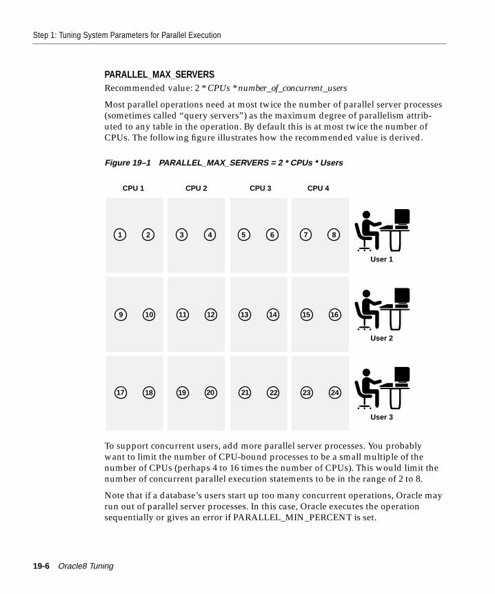
Step 1: Tuning System Parameters for Parallel Execution
PARALLEL_MAX_SERVERSRecommended value: 2 * CPUs * number_of_concurrent_users
Most parallel operations need at most twice the number of parallel server processes(sometimes called “query servers”) as the maximum degree of parallelism attrib-uted to any table in the operation. By default this is at most twice the number ofCPUs. The following figure illustrates how the recommended value is derived.
Figure 19–1 PARALLEL_MAX_SERVERS = 2 * CPUs * Users
To support concurrent users, add more parallel server processes. You probablywant to limit the number of CPU-bound processes to be a small multiple of thenumber of CPUs (perhaps 4 to 16 times the number of CPUs). This would limit thenumber of concurrent parallel execution statements to be in the range of 2 to 8.
Note that if a database’s users start up too many concurrent operations, Oracle mayrun out of parallel server processes. In this case, Oracle executes the operationsequentially or gives an error if PARALLEL_MIN_PERCENT is set.
User 3
User 2
User 1
7 8
15 16
23 24
5 6
13 14
21 22
3 4
11 12
19 20
1 2
9 10
17 18
CPU 4CPU 3CPU 2CPU 1
19-6 Oracle8 Tuning
Step 1: Tuning System Parameters for Parallel Execution
When concurrent users use too many parallel server processes, memory contention(paging), I/O contention, or excessive context switching can occur. This contentioncould reduce system throughput to a level lower than if no parallel execution wereused. Increase the PARALLEL_MAX_SERVERS value only if your system has suffi-cient memory and I/O bandwidth for the resulting load. Limiting the total numberof parallel server processes may restrict the number of concurrent users that canexecute parallel operations, but system throughput will tend to remain stable.
To increase the number of concurrent users, you could restrict the number of con-current sessions that various classes of user can have. For example:
■ You can set a large limit for users running batch jobs.
■ You could set a medium limit for users performing analyses.
■ You could prohibit a particular class of user from using parallelism at all.
You can limit the amount of parallelism available to a given user by setting up aresource profile associated with the user. In this way you can limit the number ofsessions or concurrent logons, which limits the number of parallel processes theuser can have. (Each parallel server process working on your parallel executionstatement is logged on as you—it counts against your limit of concurrent sessions.)For example, to limit a user to 10 processes, the DBA would set the user’s limit to11: one process for the parallel coordinator, and ten more parallel processes whichwould consist of two server sets. The user’s maximum degree of parallelism wouldthus be 5.
On Oracle Parallel Server, if you have reached the limit ofPARALLEL_MAX_SERVERS on an instance and you attempt to query a GV$ view,one additional parallel server process will be spawned for this purpose. The extraprocess is not available for any parallel operation other than GV$ queries.
See Also: "The Formula for Memory, Users, and Parallel Server Processes" on page20-2 for further information on balancing concurrent users, degree of parallelism,and resources consumed.Oracle8 Administrator’s Guide for more information about managing resources withuser profiles.Oracle8 Parallel Server Concepts & Administration for more information on queryingGV$ views.
Tuning Parallel Execution 19-7
Step 1: Tuning System Parameters for Parallel Execution
PARALLEL_MIN_SERVERSRecommended value: PARALLEL_MAX_SERVERS
The system parameter PARALLEL_MIN_SERVERS allows you to specify the num-ber of processes to be started and reserved for parallel operations at startup in a sin-gle instance. The syntax is:
PARALLEL_MIN_SERVERS=n
where n is the number of processes you want to start and reserve for parallel opera-tions. Sometimes you may not be able to increase the maximum number of parallelserver processes for an instance, because the maximum number depends on thecapacity of the CPUs and the I/O bandwidth (platform-specific issues). However, ifservers are continuously starting and shutting down, you should consider increas-ing the value of the parameter PARALLEL_MIN_SERVERS.
For example, if you have determined that the maximum number of concurrent par-allel server processes that your machine can manage is 100, you should setPARALLEL_MAX_SERVERS to 100. Next determine how many parallel server pro-cesses the average operation needs, and how many operations are likely to be exe-cuted concurrently. For this example, assume you will have two concurrentoperations with 20 as the average degree of parallelism. At any given time, therecould be 80 parallel server processes busy on an instance. You should therefore setthe parameter PARALLEL_MIN_SERVERS to 80.
Consider decreasing PARALLEL_MIN_SERVERS if fewer parallel server processesthan this value are typically busy at any given time. Idle parallel server processesconstitute unnecessary system overhead.
Consider increasing PARALLEL_MIN_SERVERS if more parallel server processesthan this value are typically active, and the “Servers Started” statistic ofV$PQ_SYSSTAT is continuously growing.
The advantage of starting these processes at startup is the reduction of process cre-ation overhead. Note that Oracle reserves memory from the shared pool for theseprocesses; you should therefore add additional memory using the initializationparameter SHARED_POOL_SIZE to compensate. Use the following formula todetermine how much memory to add:
(CPUs + 2) * (PARALLEL_MIN_SERVERS) * 1.5 * (BLOCK_SIZE)
19-8 Oracle8 Tuning
Step 1: Tuning System Parameters for Parallel Execution
PARALLEL_ADAPTIVE_MULTI_USERRecommended value: FALSE
On sites that have no clear usage profile, no consistent pattern of usage, you canuse the PARALLEL_ADAPTIVE_MULTI_USER parameter to tune parallel execu-tion for a multi-user environment. When set to TRUE, this parameter automaticallyreduces the requested degree of parallelism based on the current number of activeparallel execution users on the system. The effective degree of parallelism is basedon the degree of parallelism set by the table attributes or hint, divided by the totalnumber of parallel execution users. Oracle assumes that the degree of parallelismprovided has been tuned for optimal performance in a single user environment.
Note: This approach may not be suited for the general tuning policies you haveimplemented at your site. For this reason you should test and understand itseffects, given your normal workload, before deciding to use it.
Note in particular that the degree of parallelism is not dynamic, but adaptive. Itworks best during a steady state when the number of users remains fairly constant.When the number of users increases or decreases drastically, the machine may beover- or under-utilized. For best results, use a parallel degree which is slightlygreater than the number of processors. Based on available memory, the system canabsorb an extra load. Once the degree of parallelism is chosen, it is kept during theentire query.
Consider, for example, a 16 CPU machine with the default degree of parallelism setto 32. If one user issues a parallel query, that user gets a degree of 32, effectively uti-lizing all of the CPU and memory resources in the system. If two users issue paral-lel queries, each gets a degree of 16. As the number of users on the systemincreases, the degree of parallelism continues to be reduced until a maximum of 32users are running with degree 1 parallelism.
This parameter works best when used in single-node symmetric multiprocessors(SMPs). However, it can be set to TRUE when using Oracle Parallel Server if all ofthe following conditions are true:
* All parallel execution users connect to the same node.
* Instance groups are not configured.
* Each node has more than one CPU.
In this case, Oracle attempts to reduce the instances first, then the degree. If any ofthe above conditions is not met, and the parameter is set to TRUE, the algorithmmay reduce parallelism excessively, causing unnecessary idle time.
Tuning Parallel Execution 19-9
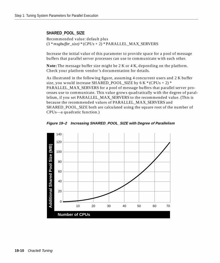
Step 1: Tuning System Parameters for Parallel Execution
SHARED_POOL_SIZERecommended value: default plus(3 * msgbuffer_size) * (CPUs + 2) * PARALLEL_MAX_SERVERS
Increase the initial value of this parameter to provide space for a pool of messagebuffers that parallel server processes can use to communicate with each other.
Note: The message buffer size might be 2 K or 4 K, depending on the platform.Check your platform vendor’s documentation for details.
As illustrated in the following figure, assuming 4 concurrent users and 2 K buffersize, you would increase SHARED_POOL_SIZE by 6 K * (CPUs + 2) *PARALLEL_MAX_SERVERS for a pool of message buffers that parallel server pro-cesses use to communicate. This value grows quadratically with the degree of paral-lelism, if you set PARALLEL_MAX_SERVERS to the recommended value. (This isbecause the recommended values of PARALLEL_MAX_SERVERS andSHARED_POOL_SIZE both are calculated using the square root of the number ofCPUs—a quadratic function.)
Figure 19–2 Increasing SHARED_POOL_SIZE with Degree of Parallelism
Number of CPUs
Ad
dit
ion
al S
har
ed P
oo
l Siz
e (M
B)
10 20 30 40 50 60 700
20
40
60
80
100
120
140
19-10 Oracle8 Tuning

Step 1: Tuning System Parameters for Parallel Execution
Parallel plans take up about twice as much space in the SQL area as serial plans,but additional space allocation is probably not necessary because generally they arenot shared.
On Oracle Parallel Server, multiple CPUs can exist in a single node, and paralleloperation can be performed across nodes. Whereas symmetric multiprocessor(SMP) systems use 3 buffers for connection, 4 buffers are used to connect betweeninstances on Oracle Parallel Server. Thus you should normally have 4 buffers inshared memory: 2 in the local shared pool and 2 in the remote shared pool. The for-mula for increasing the value of SHARED_POOL_SIZE on Oracle Parallel Serverbecomes:
(4 * msgbuffer_size) * ((CPUs_per_node * #nodes ) + 2) * (PARALLEL_MAX_SERVERS * #nodes)
Note that the degree of parallelism on Oracle Parallel Server is expressed by thenumber of CPUs per node multiplied by the number of nodes.
Tuning Parallel Execution 19-11
Step 1: Tuning System Parameters for Parallel Execution
SORT_AREA_SIZESample Range: 256 K to 4 M
This parameter specifies the amount of memory to allocate per parallel server pro-cess for sort operations. If memory is abundant on your system, you can benefitfrom setting SORT_AREA_SIZE to a large value. This can dramatically increase theperformance of hash operations, because the entire operation is more likely to beperformed in memory. However, if memory is a concern for your system, you maywant to limit the amount of memory allocated for sorts and hashing operations.Instead, increase the size of the buffer cache so that data blocks from temporarysort segments can be cached in the buffer cache.
If the sort area is too small, an excessive amount of I/O will be required to merge alarge number of runs. If the sort area size is smaller than the amount of data to sort,then the sort will spill to disk, creating sort runs. These must then be merged againusing the sort area. If the sort area size is very small, there will be many runs tomerge, and multiple passes may be necessary. The amount of I/O increases as thesort area size decreases.
If the sort area is too large, the operating system paging rate will be excessive. Thecumulative sort area adds up fast, because each parallel server can allocate thisamount of memory for each sort. Monitor the operating system paging rate to see iftoo much memory is being requested.
Note that SORT_AREA_SIZE is relevant to parallel query operations and to thequery portion of DML or DDL statements. All CREATE INDEX statements must dosome sorting to generate the index. These include:
■ CREATE INDEX
■ direct-load INSERT (if an index is involved)
■ ALTER INDEX ... REBUILD
See Also: "HASH_AREA_SIZE" on page 19-4
19-12 Oracle8 Tuning
Step 1: Tuning System Parameters for Parallel Execution
Parameters Affecting Resource Consumption for Parallel DML & Parallel DDLParallel INSERT, UPDATE, and DELETE require more resources than do serialDML operations. Likewise, PARALLEL CREATE TABLE ... AS SELECT and PAR-ALLEL CREATE INDEX may require more resources. For this reason you mayneed to increase the value of several additional initialization parameters. Note thatthese parameters do not affect resources for queries.
See Also: Oracle8 SQL Reference for complete information about parameters.
TRANSACTIONSFor parallel DML, each parallel server process starts a transaction. The parallel coor-dinator uses the two-phase commit protocol to commit transactions; therefore thenumber of transactions being processed increases by the degree of parallelism. Youmay thus need to increase the value of the TRANSACTIONS initialization parame-ter, which specifies the maximum number of concurrent transactions. (The defaultassumes no parallelism.) For example, if you have degree 20 parallelism you willhave 20 more new server transactions (or 40, if you have two server sets) and 1coordinator transaction; thus you should increase TRANSACTIONS by 21 (or 41), ifthey are running in the same instance.
ROLLBACK_SEGMENTSThe increased number of transactions for parallel DML necessitates many rollbacksegments. For example, one command with degree 5 parallelism uses 5 server trans-actions, which should be distributed among different rollback segments. The roll-back segments should belong to tablespaces that have free space. The rollbacksegments should be unlimited, or you should specify a high value for the MAXEX-TENTS parameter of the STORAGE clause. In this way they can extend and not runout of space.
LOG_BUFFERCheck the statistic “redo buffer allocation retries” in the V$SYSSTAT view. If thisvalue is high, try to increase the LOG_BUFFER size. A common LOG_BUFFER sizefor a system generating lots of logs is 3 to 5MB. If the number of retries is still highafter increasing LOG_BUFFER size, a problem may exist with the disk where thelog buffers reside. In that case, stripe the log files across multiple disks in order toincrease the I/O bandwidth.
Note that parallel DML generates a good deal more redo than does serial DML,especially during inserts, updates and deletes.
Tuning Parallel Execution 19-13
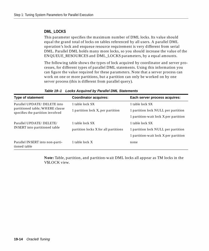
Step 1: Tuning System Parameters for Parallel Execution
DML_LOCKSThis parameter specifies the maximum number of DML locks. Its value shouldequal the grand total of locks on tables referenced by all users. A parallel DMLoperation’s lock and enqueue resource requirement is very different from serialDML. Parallel DML holds many more locks, so you should increase the value of theENQUEUE_RESOURCES and DML_LOCKS parameters, by a equal amounts.
The following table shows the types of lock acquired by coordinator and server pro-cesses, for different types of parallel DML statements. Using this information youcan figure the value required for these parameters. Note that a server process canwork on one or more partitions, but a partition can only be worked on by oneserver process (this is different from parallel query).
Note: Table, partition, and partition-wait DML locks all appear as TM locks in theV$LOCK view.
Table 19–1 Locks Acquired by Parallel DML Statements
Type of statement Coordinator acquires: Each server process acquires:
Parallel UPDATE/DELETE intopartitioned table; WHERE clausespecifies the partition involved
1 table lock SX
1 partition lock X, per partition
1 table lock SX
1 partition lock NULL per partition
1 partition-wait lock X per partition
Parallel UPDATE/DELETE/INSERT into partitioned table
1 table lock SX
partition locks X for all partitions
1 table lock SX
1 partition lock NULL per partition
1 partition-wait lock X per partition
Parallel INSERT into non-parti-tioned table
1 table lock X none
19-14 Oracle8 Tuning
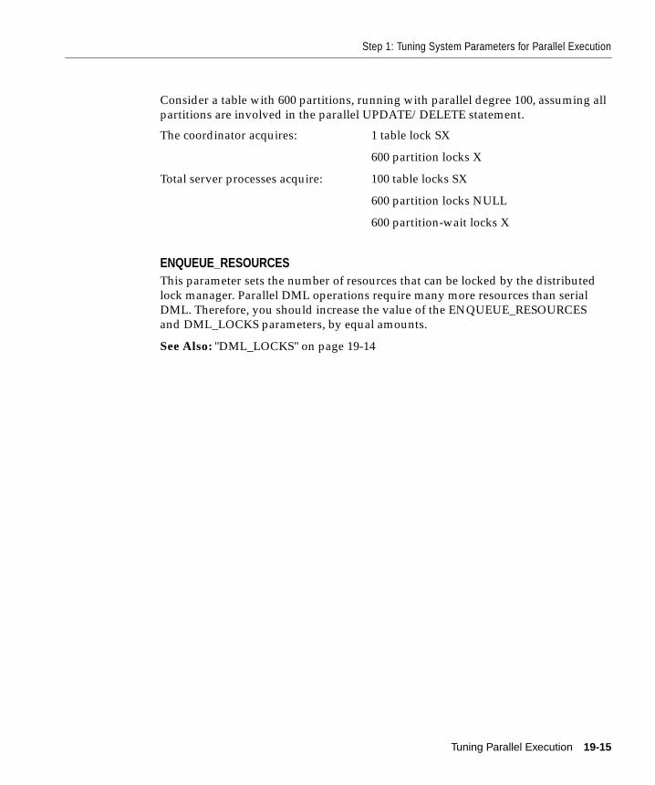
Step 1: Tuning System Parameters for Parallel Execution
Consider a table with 600 partitions, running with parallel degree 100, assuming allpartitions are involved in the parallel UPDATE/DELETE statement.
ENQUEUE_RESOURCESThis parameter sets the number of resources that can be locked by the distributedlock manager. Parallel DML operations require many more resources than serialDML. Therefore, you should increase the value of the ENQUEUE_RESOURCESand DML_LOCKS parameters, by equal amounts.
See Also: "DML_LOCKS" on page 19-14
The coordinator acquires: 1 table lock SX
600 partition locks X
Total server processes acquire: 100 table locks SX
600 partition locks NULL
600 partition-wait locks X
Tuning Parallel Execution 19-15
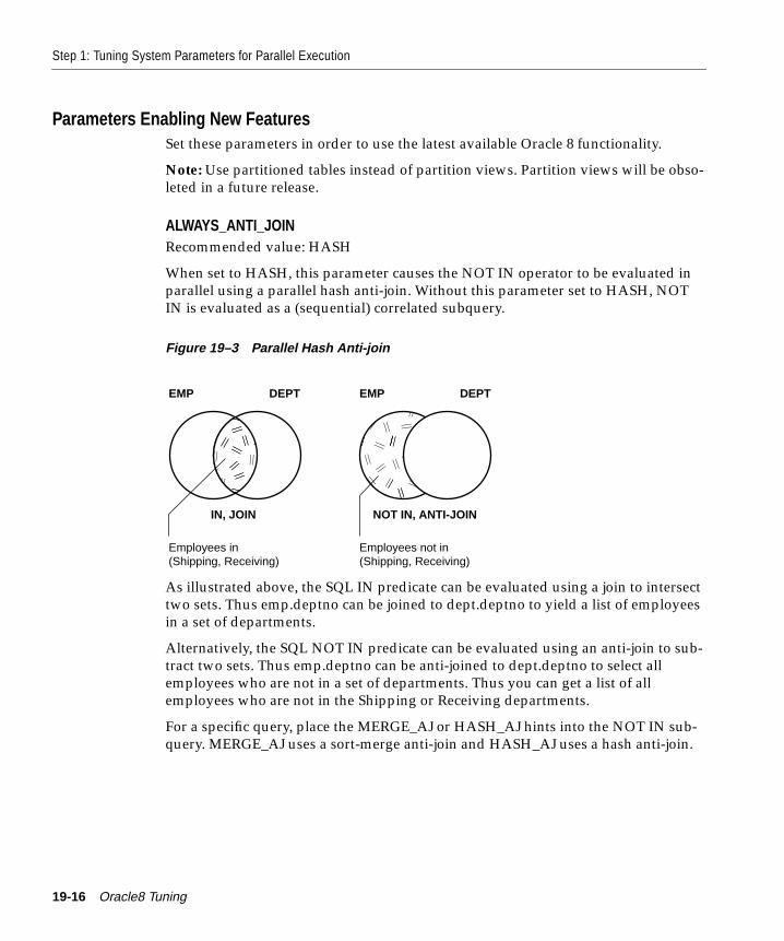
Step 1: Tuning System Parameters for Parallel Execution
Parameters Enabling New FeaturesSet these parameters in order to use the latest available Oracle 8 functionality.
Note: Use partitioned tables instead of partition views. Partition views will be obso-leted in a future release.
ALWAYS_ANTI_JOINRecommended value: HASH
When set to HASH, this parameter causes the NOT IN operator to be evaluated inparallel using a parallel hash anti-join. Without this parameter set to HASH, NOTIN is evaluated as a (sequential) correlated subquery.
Figure 19–3 Parallel Hash Anti-join
As illustrated above, the SQL IN predicate can be evaluated using a join to intersecttwo sets. Thus emp.deptno can be joined to dept.deptno to yield a list of employeesin a set of departments.
Alternatively, the SQL NOT IN predicate can be evaluated using an anti-join to sub-tract two sets. Thus emp.deptno can be anti-joined to dept.deptno to select allemployees who are not in a set of departments. Thus you can get a list of allemployees who are not in the Shipping or Receiving departments.
For a specific query, place the MERGE_AJ or HASH_AJ hints into the NOT IN sub-query. MERGE_AJ uses a sort-merge anti-join and HASH_AJ uses a hash anti-join.
EMP DEPT EMP DEPT
IN, JOIN NOT IN, ANTI-JOIN������ ���������Employees in
(Shipping, Receiving)Employees not in (Shipping, Receiving)
19-16 Oracle8 Tuning
Step 1: Tuning System Parameters for Parallel Execution
For example:
SELECT * FROM empWHERE ename LIKE ’J%’ ANDdeptno IS NOT NULL ANDdeptno NOT IN (SELECT /*+ HASH_AJ */ deptno FROM deptWHERE deptno IS NOT NULL ANDloc = ’DALLAS’);
If you wish the anti-join transformation always to occur if the conditions in the pre-vious section are met, set the ALWAYS_ANTI_JOIN initialization parameter toMERGE or HASH. The transformation to the corresponding anti-join type thentakes place whenever possible.
ALWAYS_SEMI_JOINRecommended value: default
When set to HASH, this parameter converts a correlated EXISTS subquery into aview query block and semi-join which is evaluated in parallel.
For a specific query, place the HASH_SJ or MERGE_SJ hint into the EXISTS sub-query. HASH_SJ uses a hash semi-join and MERGE_SJ uses a sort merge semi-join.For example:
SELECT * FROM t1WHERE EXISTS (SELECT /*+ HASH_SJ */ * FROM t2
WHERE t1.c1 = t2.c1AND t2.c3 > 5);
This converts the subquery into a special type of join between t1 and t2 that pre-serves the semantics of the subquery; that is, even if there is more than one match-ing row in t2 for a row in t1, the row in t1 will be returned only once.
A subquery will be evaluated as a semi-join only with the following limitations:
■ There can only be one table in the subquery.
■ The outer query block must not itself be a subquery.
■ The subquery must be correlated with an equality predicate.
■ The subquery must have no GROUP BY, CONNECT BY, or rownum references.
If you wish the semi-join transformation always to occur if the conditions in the pre-vious section are met, set the ALWAYS_SEMI_JOIN initialization parameter toHASH or MERGE. The transformation to the corresponding semi-join type thentakes place whenever possible.
Tuning Parallel Execution 19-17
Step 1: Tuning System Parameters for Parallel Execution
COMPATIBLESample Value: 8.0.0
This parameter enables new features that may prevent you from falling back to anearlier release. To be sure that you are getting the full benefit of the latest perfor-mance features, set this parameter equal to the current release.
Note: Make a full backup before you change the value of this parameter.
PARALLEL_BROADCAST_ENABLERecommended value: default
You can set this parameter to TRUE if you are joining a very large join result setwith a very small result set (size being measured in bytes, rather than number ofrows). In this case, the optimizer has the option of broadcasting the row sources ofthe small result set, such that a single table queue will send all of the small set’srows to each of the parallel servers which are processing the rows of the larger set.The result is enhanced performance.
Note that this parameter, which cannot be set dynamically, affects only hash joinsand merge joins.
19-18 Oracle8 Tuning
Step 1: Tuning System Parameters for Parallel Execution
Parameters Related to I/OTune the following parameters to ensure that I/O operations are optimized for par-allel execution.
DB_BLOCK_BUFFERSWhen you perform parallel updates and deletes, the buffer cache behavior is verysimilar to any system running a high volume of updates. For more information see"Tuning the Buffer Cache" on page 14-26.
DB_BLOCK_SIZERecommended value: 8K or 16K
The database block size must be set when the database is created. If you are creat-ing a new database, use a large block size.
DB_FILE_MULTIBLOCK_READ_COUNTRecommended value: 8, for 8K block size; 4, for 16K block size
This parameter determines how many database blocks are read with a single oper-ating system READ call. Many platforms limit the number of bytes read to 64K, lim-iting the effective maximum for an 8K block size to 8. Other platforms have ahigher limit. For most applications, 64K is acceptable. In general, use the formula:
DB_FILE_MULTIBLOCK_READ_COUNT = 64K/DB_BLOCK_SIZE.
HASH_MULTIBLOCK_IO_COUNTRecommended value: 4
This parameter specifies how many blocks a hash join reads and writes at once.Increasing the value of HASH_MULTIBLOCK_IO_COUNT decreases the numberof hash buckets. If a system is I/O bound, you can increase the efficiency of I/O byhaving larger transfers per I/O.
Because memory for I/O buffers comes from the HASH_AREA_SIZE, larger I/Obuffers mean fewer hash buckets. There is a trade-off, however. For large tables(hundreds of gigabytes in size) it is better to have more hash buckets and slightlyless efficient I/Os. If you find an I/O bound condition on temporary space duringhash join, consider increasing the value of HASH_MULTIBLOCK_IO_COUNT.
Tuning Parallel Execution 19-19

Step 1: Tuning System Parameters for Parallel Execution
PARALLEL_EXECUTION_MESSAGE_SIZERecommended value: default
This parameter specifies the size of messages for parallel execution. The defaultvalue, which is operating system specific, should be adequate for most applica-tions. Larger values would require a larger shared pool.
SORT_DIRECT_WRITESRecommended value: AUTO
When this parameter is set to AUTO and SORT_AREA_SIZE is greater than 10times the buffer size, this parameter causes the buffer cache to be bypassed for thewriting of sort runs.
Reading through the buffer cache may result in greater path length, excessive mem-ory bus utilization, and LRU latch contention on SMPs. Avoiding the buffer cachecan thus provide performance improvement by a factor of 3 or more. It alsoremoves the need to tune buffer cache and DBWn parameters.
Excessive paging is a symptom that the relationship of memory, users, and parallelserver processes is out of balance. To rebalance it, you can reduce the sort or hasharea size. You can limit the amount of memory for sorts if SORT_DIRECT_WRITESis set to AUTO but the SORT_AREA_SIZE is small. Then sort blocks will be cachedin the buffer cache. Note that SORT_DIRECT_WRITES has no effect on hashing.
See Also: "HASH_AREA_SIZE" on page 19-4
SORT_READ_FACRecommended value: depends on disk speed
This value is a ratio that sets the amount of time needed to read a single databaseblock, divided by the block transfer rate.
See Also: Oracle8 Reference and your Oracle platform-specific documentation formore information about setting this parameter.
19-20 Oracle8 Tuning
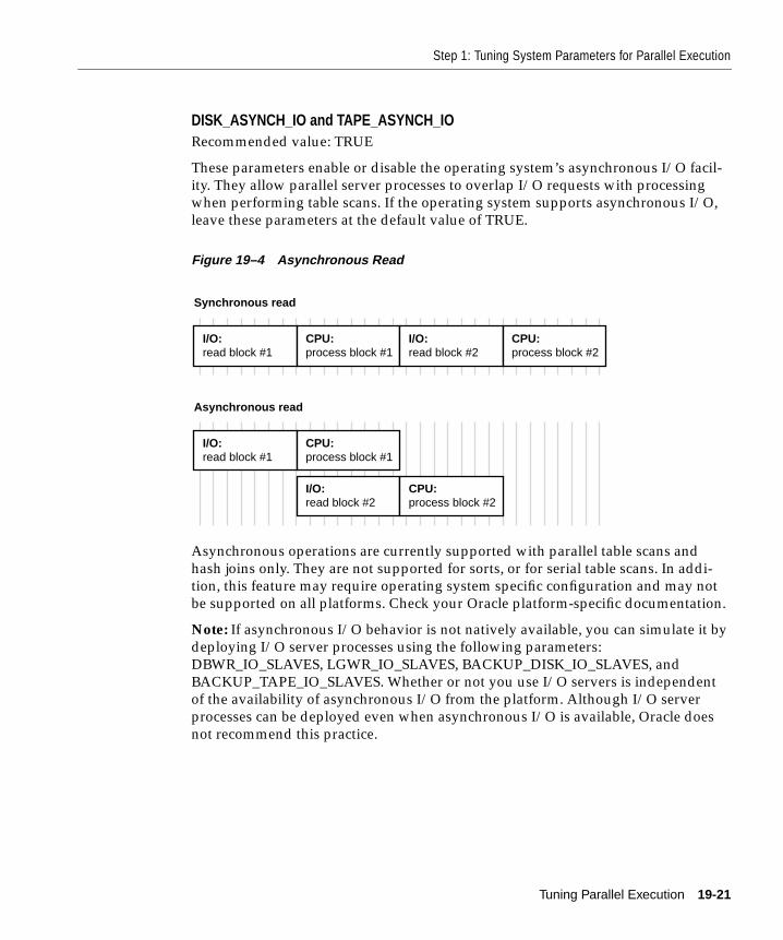
Step 1: Tuning System Parameters for Parallel Execution
DISK_ASYNCH_IO and TAPE_ASYNCH_IORecommended value: TRUE
These parameters enable or disable the operating system’s asynchronous I/O facil-ity. They allow parallel server processes to overlap I/O requests with processingwhen performing table scans. If the operating system supports asynchronous I/O,leave these parameters at the default value of TRUE.
Figure 19–4 Asynchronous Read
Asynchronous operations are currently supported with parallel table scans andhash joins only. They are not supported for sorts, or for serial table scans. In addi-tion, this feature may require operating system specific configuration and may notbe supported on all platforms. Check your Oracle platform-specific documentation.
Note: If asynchronous I/O behavior is not natively available, you can simulate it bydeploying I/O server processes using the following parameters:DBWR_IO_SLAVES, LGWR_IO_SLAVES, BACKUP_DISK_IO_SLAVES, andBACKUP_TAPE_IO_SLAVES. Whether or not you use I/O servers is independentof the availability of asynchronous I/O from the platform. Although I/O serverprocesses can be deployed even when asynchronous I/O is available, Oracle doesnot recommend this practice.
I/O: read block #1
CPU: process block #1
I/O: read block #2
CPU: process block #2
Synchronous read
I/O: read block #1
CPU: process block #1
I/O: read block #2
CPU: process block #2
Asynchronous read
Tuning Parallel Execution 19-21
Step 2: Tuning Physical Database Layout for Parallel Execution
Step 2: Tuning Physical Database Layout for Parallel ExecutionThis section describes how to tune the physical database layout for optimal perfor-mance of parallel execution.
■ Types of Parallelism
■ Striping Data
■ Partitioning Data
■ Determining the Degree of Parallelism
■ Populating the Database Using Parallel Load
■ Setting Up Temporary Tablespaces for Parallel Sort and Hash Join
■ Creating Indexes in Parallel
■ Additional Considerations for Parallel DML Only
Types of ParallelismDifferent parallel operations use different types of parallelism. The physical data-base layout you choose should depend on what parallel operations are most preva-lent in your application.
The basic unit of parallelism is a called a granule. The operation being parallelized(a table scan, table update, or index creation, for example) is divided by Oracle intogranules. Parallel server processes execute the operation one granule at a time. Thenumber of granules and their size affect the degree of parallelism you can use, andhow well the work is balanced across parallel server processes.
Block Range GranulesBlock range granules are the basic unit of most parallel operations (exceptionsinclude such operations as parallel DML and CREATE LOCAL INDEX). This istrue even on partitioned tables; it is the reason why, on Oracle, the parallel degreeis not related to the number of partitions. Block range granules are ranges of physi-cal blocks from the table. Because they are based on physical data addresses, youcan size block range granules to allow better load balancing. Block range granulespermit dynamic parallelism that does not depend on static preallocation of tablesor indexes. On SMP systems granules are located on different devices in order todrive as many disks as possible. On many MPP systems, block range granules arepreferentially assigned to parallel server processes that have physical proximity tothe disks storing the granules. Block range granules are used with global striping.
19-22 Oracle8 Tuning
Step 2: Tuning Physical Database Layout for Parallel Execution
When block range granules are used predominantly for parallel access to a table orindex, administrative considerations such as recovery, or using partitions for delet-ing portions of data, may influence partition layout more than performance consid-erations. If parallel execution operations frequently take advantage of partitionpruning, it is important that the set of partitions accessed by the query be stripedover at least as many disks as the degree of parallelism.
See Also: For MPP systems, see your platform-specific documentation
Partition GranulesWhen partition granules are used, a parallel server process works on an entire parti-tion of a table or index. Because partition granules are statically determined when atable or index is created, partition granules do not allow as much flexibility in paral-lelizing an operation. This means that the degree of parallelism possible might belimited, and that load might not be well balanced across parallel server processes.
Partition granules are the basic unit of parallel index range scans and parallel opera-tions that modify multiple partitions of a partitioned table or index. These opera-tions include parallel update, parallel delete, parallel direct-load insert intopartitioned tables, parallel creation of partitioned indexes, and parallel creation ofpartitioned tables.
When partition granules are used for parallel access to a table or index, it is impor-tant that there be a relatively large number of partitions (at least three times thedegree of parallelism), so that work can be balanced across the parallel server pro-cesses.
See Also: Oracle8 Concepts for information on disk striping and partitioning.
Tuning Parallel Execution 19-23
Step 2: Tuning Physical Database Layout for Parallel Execution
Striping DataTo avoid I/O bottlenecks, you should stripe all tablespaces accessed in parallelover at least as many disks as the degree of parallelism. Stripe over at least as manydevices as CPUs. You should stripe tablespaces for tables, tablespaces for indexes,and temporary tablespaces. You must also spread the devices over controllers, I/Ochannels, and/or internal busses.
Figure 19–5 Striping Objects Over at Least as Many Devices as CPUs
To stripe data during load, use the FILE= clause of parallel loader to load data frommultiple load sessions into different files in the tablespace. For any striping to beeffective, you must ensure that enough controllers and other I/O components areavailable to support the bandwidth of parallel data movement into and out of thestriped tablespaces.
The operating system or volume manager can perform striping (OS striping), oryou can perform striping manually for parallel operations.
Operating system striping with a large stripe size (at least 64K) is recommended,when possible. This approach always performs better than manual striping, espe-cially in multi-user environments.
4
0001
0002
tablespace 1
3
2
1
tablespace 2
tablespace 3
tablespace 44
0001
0002
3
2
1
4
0001
0002
3
2
1
4
0001
0002
3
2
1
Controller 2Controller 1
19-24 Oracle8 Tuning
Step 2: Tuning Physical Database Layout for Parallel Execution
Operating System StripingOperating system striping is usually flexible and easy to manage. It supports multi-ple users running sequentially as well as single users running in parallel. Two mainadvantages make OS striping preferable to manual striping, unless the system isvery small or availability is the main concern:
■ For parallel scan operations (such as full table scan or fast full scan), operatingsystem striping increases the number of disk seeks. Nevertheless, this is largelycompensated by the large I/O size (DB_BLOCK_SIZE *MULTIBLOCK_READ_COUNT), which should enable this operation to reachthe maximum I/O throughput that your platform can deliver. Note that thismaximum is in general limited by the number of controllers or I/O buses of theplatform, not by the number of disks (unless you have a very small configura-tion).
■ For index probes (for example, within a nested loop join or parallel index rangescan), operating system striping enables you to avoid hot spots: I/O will bemore evenly distributed across the disks.
Stripe size must be at least as large as the I/O size. If stripe size is larger than I/Osize by a factor of 2 or 4, then certain tradeoffs may arise. The large stripe size canbe beneficial because it allows the system to perform more sequential operations oneach disk; it decreases the number of seeks on disk. The disadvantage is that itreduces the I/O parallelism so that fewer disks are active at the same time. If youshould encounter problems in this regard, increase the I/O size of scan operations(going, for example, from 64K to 128K), rather than changing the stripe size. Notethat the maximum I/O size is platform specific (in a range, for example, of 64K to1MB).
With OS striping, from a performance standpoint, the best layout is to stripe data,indexes, and temporary tablespaces across all the disks of your platform. In thisway, maximum I/O performance (both in term of throughput and number of I/Osper second) can be reached when one object is accessed by a parallel operation. Ifmultiple objects are accessed at the same time (as in a multi-user configuration),striping will automatically limit the contention. If availability is a major concern,associate this scheme with hardware redundancy (for example RAID5), which per-mits both performance and availability.
Tuning Parallel Execution 19-25
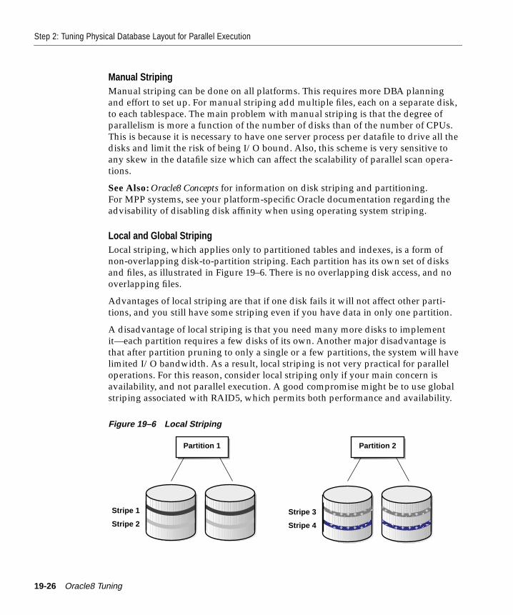
Step 2: Tuning Physical Database Layout for Parallel Execution
Manual StripingManual striping can be done on all platforms. This requires more DBA planningand effort to set up. For manual striping add multiple files, each on a separate disk,to each tablespace. The main problem with manual striping is that the degree ofparallelism is more a function of the number of disks than of the number of CPUs.This is because it is necessary to have one server process per datafile to drive all thedisks and limit the risk of being I/O bound. Also, this scheme is very sensitive toany skew in the datafile size which can affect the scalability of parallel scan opera-tions.
See Also: Oracle8 Concepts for information on disk striping and partitioning.For MPP systems, see your platform-specific Oracle documentation regarding theadvisability of disabling disk affinity when using operating system striping.
Local and Global StripingLocal striping, which applies only to partitioned tables and indexes, is a form ofnon-overlapping disk-to-partition striping. Each partition has its own set of disksand files, as illustrated in Figure 19–6. There is no overlapping disk access, and nooverlapping files.
Advantages of local striping are that if one disk fails it will not affect other parti-tions, and you still have some striping even if you have data in only one partition.
A disadvantage of local striping is that you need many more disks to implementit—each partition requires a few disks of its own. Another major disadvantage isthat after partition pruning to only a single or a few partitions, the system will havelimited I/O bandwidth. As a result, local striping is not very practical for paralleloperations. For this reason, consider local striping only if your main concern isavailability, and not parallel execution. A good compromise might be to use globalstriping associated with RAID5, which permits both performance and availability.
Figure 19–6 Local Striping
Stripe 1
Stripe 2
Partition 1 Partition 2
Stripe 3
Stripe 4������������
19-26 Oracle8 Tuning������
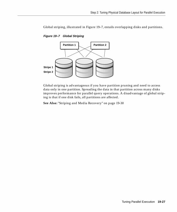
Step 2: Tuning Physical Database Layout for Parallel Execution
Global striping, illustrated in Figure 19–7, entails overlapping disks and partitions.
Figure 19–7 Global Striping
Global striping is advantageous if you have partition pruning and need to accessdata only in one partition. Spreading the data in that partition across many disksimproves performance for parallel query operations. A disadvantage of global strip-ing is that if one disk fails, all partitions are affected.
See Also: "Striping and Media Recovery" on page 19-30
Stripe 1
Stripe 2
Partition 1 Partition 2
Tuning Parallel Execution 19-27
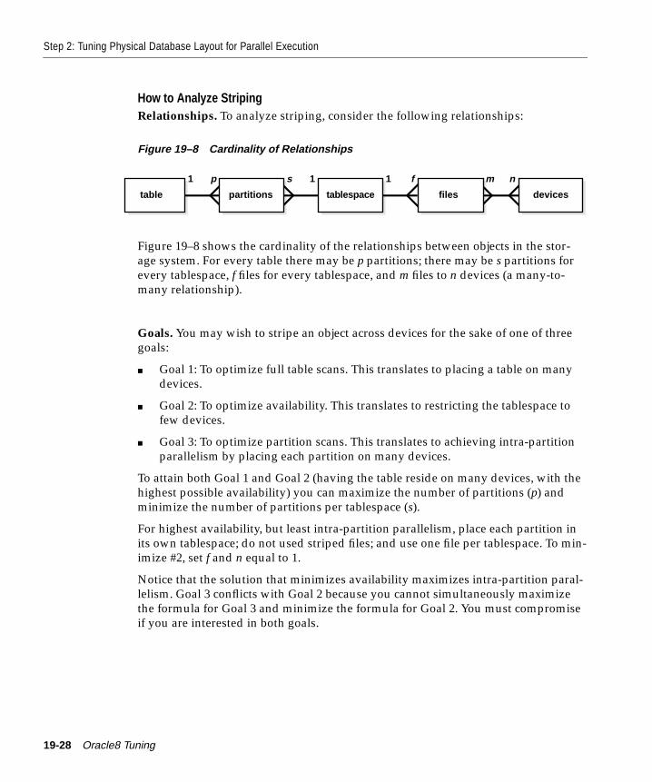
Step 2: Tuning Physical Database Layout for Parallel Execution
How to Analyze StripingRelationships. To analyze striping, consider the following relationships:
Figure 19–8 Cardinality of Relationships
Figure 19–8 shows the cardinality of the relationships between objects in the stor-age system. For every table there may be p partitions; there may be s partitions forevery tablespace, f files for every tablespace, and m files to n devices (a many-to-many relationship).
Goals. You may wish to stripe an object across devices for the sake of one of threegoals:
■ Goal 1: To optimize full table scans. This translates to placing a table on manydevices.
■ Goal 2: To optimize availability. This translates to restricting the tablespace tofew devices.
■ Goal 3: To optimize partition scans. This translates to achieving intra-partitionparallelism by placing each partition on many devices.
To attain both Goal 1 and Goal 2 (having the table reside on many devices, with thehighest possible availability) you can maximize the number of partitions (p) andminimize the number of partitions per tablespace (s).
For highest availability, but least intra-partition parallelism, place each partition inits own tablespace; do not used striped files; and use one file per tablespace. To min-imize #2, set f and n equal to 1.
Notice that the solution that minimizes availability maximizes intra-partition paral-lelism. Goal 3 conflicts with Goal 2 because you cannot simultaneously maximizethe formula for Goal 3 and minimize the formula for Goal 2. You must compromiseif you are interested in both goals.
table partitions tablespace devicesfiles
1 p s 1 1 f m n
19-28 Oracle8 Tuning

Step 2: Tuning Physical Database Layout for Parallel Execution
Goal 1: To optimize full table scans. Having a table on many devices is beneficialbecause full table scans are scalable.
Calculate the number of partitions multiplied by the number of files in thetablespace multiplied by the number of devices per file. Divide this product by thenumber of partitions that share the same tablespace, multiplied by the number offiles that share the same device. The formula is as follows:
You can do this by having t partitions, with every partition in its own tablespace, ifevery tablespace has one file, and these files are not striped.
t x 1/p x 1 x 1, up to t devices
If the table is not partitioned, but is in one tablespace, one file, it should be stripedover n devices.
1 x 1 x n
Maximum t partitions, every partition in its own tablespace, f files in eachtablespace, each tablespace on striped device:
t x f x n devices
Goal 2: To optimize availability. Restricting each tablespace to a small number ofdevices and having as many partitions as possible helps you achieve high availabil-ity.
Availability is maximized when f = n = m = 1 and p is much greater than 1.
Goal 3: To optimize partition scans. Achieving intra-partition parallelism is benefi-cial because partition scans are scalable. To do this, place each partition on manydevices.
Partitions can reside in a tablespace that can have many files. There could be either
■ many files per tablespace, or
■ striped file
Number of devices per table = p • f • ns • m
Number of devices per tablespace = f • nm
Number of devices per partition = f • ns • m
Tuning Parallel Execution 19-29
Step 2: Tuning Physical Database Layout for Parallel Execution
Striping and Media RecoveryStriping affects media recovery. Loss of a disk usually means loss of access to allobjects that were stored on that disk. If all objects are striped over all disks, thenloss of any disk takes down the entire database. Furthermore, you may need torestore all database files from backups, even if each file has only a small fractionactually stored on the failed disk.
Often, the same OS subsystem that provides striping also provides mirroring. Withthe declining price of disks, mirroring can provide an effective supplement to back-ups and log archival--but not a substitute for them. Mirroring can help your systemrecover from a device failure more quickly than with a backup, but is not as robust.Mirroring does not protect against software faults and other problems that an inde-pendent backup would protect your system against. Mirroring can be used effec-tively if you are able to reload read-only data from the original source tapes. If youdo have a disk failure, restoring the data from the backup could involve lengthydowntime, whereas restoring it from a mirrored disk would enable your system toget back online quickly.
Even cheaper than mirroring is RAID technology, which avoids full duplication infavor of more expensive write operations. For read-mostly applications, this maysuffice.
Note: RAID5 technology is particularly slow on write operations. This slownessmay affect your database restore time to a point that RAID5 performance is unac-ceptable.
See Also: For a discussion of manually striping tables across datafiles, refer to"Striping Disks" on page 15-23.
For a discussion of media recovery issues, see "Backup and Recovery of the DataWarehouse" on page 6-8.
For more information about automatic file striping and tools you can use to deter-mine I/O distribution among your devices, refer to your operating system docu-mentation.
19-30 Oracle8 Tuning
Step 2: Tuning Physical Database Layout for Parallel Execution
Partitioning DataPartitioned tables and indexes can improve the performance of operations in a datawarehouse. Partitioned tables and indexes allow at least the same parallelism asnon-partitioned tables and indexes. In addition, partitions of a table can be prunedbased on predicates and values in the partitioning column. Range scans on parti-tioned indexes can be parallelized, and insert, update and delete operations can beparallelized.
To avoid I/O bottlenecks when not all partitions are being scanned (because somehave been eliminated), each partition should be spread over a number of devices.On MPP systems, those devices should be spread over multiple nodes.
Partitioned tables and indexes facilitate administrative operations by allowingthem to operate on subsets of data. For example, a new partition can be added, anexisting partition can be reorganized, or an old partition can be dropped with lessthan a second of interruption to a read-only application.
Consider using partitioned tables in a data warehouse when:
■ very large tables are frequently scanned by a range predicate on a column thatwould make a good partitioning column (such as ORDER_DATE orPURCHASE_DATE)
■ new data is loaded and old data is purged periodically and this can be trans-lated into an add/drop of partitions
■ administrative operations on large tables do not fit in the allotted batch window
■ there is a need for parallel DML operations
Tuning Parallel Execution 19-31
Step 2: Tuning Physical Database Layout for Parallel Execution
Determining the Degree of ParallelismIf the data being accessed by a parallel operation (after partition pruning isapplied) is spread over at least as many disks as the degree of parallelism, thenmost operations will be CPU-bound and a degree of parallelism ranging from thetotal number of CPUs to twice that number, is appropriate. Operations that tend tobe I/O bandwidth bound can benefit from a higher degree of parallelism, espe-cially if the data is spread over more disks. On sites with multiple users, you mightconsider using the PARALLEL_ADAPTIVE_MULTI_USER parameter to tune therequested degree of parallelism based on the current number of active parallel exe-cution users. The following discussion is intended more for a single user environ-ment.
Operations that tend to be I/O bandwidth bound are:
■ selecting and counting all records in a table with a very simple or nonexistentWHERE clause
■ nested loop joins using an index
Parallel operations that perform random I/O access (such as index maintenance ofparallel update and delete operations) can saturate the I/O subsystem with a highnumber of I/Os, very much like an OLTP system with high concurrency. To easethis I/O problem, the data should be spread among more devices and disk control-lers. Increasing the degree of parallelism will not help.
Oracle automatically computes the default parallel degree of a table as the mini-mum of the number of disks storing the table and the number of CPUs available. If,as recommended, you have striped objects over at least as many disks as you haveCPUs, the default parallelism will always be the number of CPUs. Warehouse oper-ations are typically CPU bound; thus the default is a good choice, especially if youare using the asynchronous readahead feature. However, because some operationsare by nature synchronous (index probes, for example) an explicit setting of the par-allel degree to twice the number of CPUs might be more appropriate. Considerreducing parallelism for objects that are frequently accessed by two or more concur-rent parallel operations.
If you find that some operations are I/O bound with the default parallelism, andyou have more disks than CPUs, you can override the usual parallelism with a hintthat increases parallelism up to the number of disks, or until the CPUs become satu-rated.
See Also: Oracle8 Concepts"PARALLEL_ADAPTIVE_MULTI_USER" on page 19-9
19-32 Oracle8 Tuning
Step 2: Tuning Physical Database Layout for Parallel Execution
Populating the Database Using Parallel LoadThis section presents a case study which illustrates how to create, load, index, andanalyze a large data warehouse fact table with partitions, in a typical star schema.This example uses SQL Loader to explicitly stripe data over 30 disks.
■ The example 120 G table is named FACTS.
■ The system is a 10 CPU shared memory computer with more than 100 diskdrives.
■ Thirty disks (4 G each) will be used for base table data, 10 disks for index, and30 disks for temporary space. Additional disks are needed for rollback seg-ments, control files, log files, possible staging area for loader flat files, and so on.
■ The FACTS table is partitioned by month into 12 logical partitions. To facilitatebackup and recovery each partition is stored in its own tablespace.
■ Each partition is spread evenly over 10 disks, so that a scan which accesses fewpartitions, or a single partition, can still proceed with full parallelism. Thusthere can be intra-partition parallelism when queries restrict data access by par-tition pruning.
■ Each disk has been further subdivided using an OS utility into 4 OS files withnames like /dev/D1.1, /dev/D1.2, ... , /dev/D30.4.
■ Four tablespaces are allocated on each group of 10 disks. To better balance I/Oand parallelize table space creation (because Oracle writes each block in a data-file when it is added to a tablespace), it is best if each of the four tablespaces oneach group of 10 disks has its first datafile on a different disk. Thus the firsttablespace has /dev/D1.1 as its first datafile, the second tablespace has /dev/D4.2 as its first datafile, and so on, as illustrated in Figure 19–9.
Tuning Parallel Execution 19-33
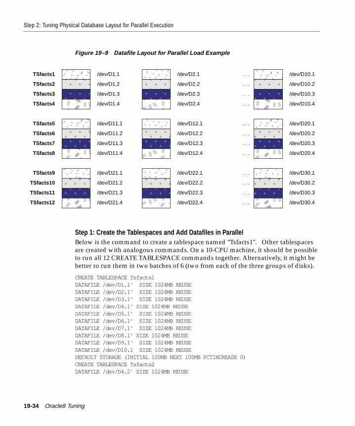
Step 2: Tuning Physical Database Layout for Parallel Execution
Figure 19–9 Datafile Layout for Parallel Load Example
Step 1: Create the Tablespaces and Add Datafiles in ParallelBelow is the command to create a tablespace named "Tsfacts1". Other tablespacesare created with analogous commands. On a 10-CPU machine, it should be possibleto run all 12 CREATE TABLESPACE commands together. Alternatively, it might bebetter to run them in two batches of 6 (two from each of the three groups of disks).
CREATE TABLESPACE Tsfacts1DATAFILE /dev/D1.1' SIZE 1024MB REUSEDATAFILE /dev/D2.1' SIZE 1024MB REUSEDATAFILE /dev/D3.1' SIZE 1024MB REUSEDATAFILE /dev/D4.1' SIZE 1024MB REUSEDATAFILE /dev/D5.1' SIZE 1024MB REUSEDATAFILE /dev/D6.1' SIZE 1024MB REUSEDATAFILE /dev/D7.1' SIZE 1024MB REUSEDATAFILE /dev/D8.1' SIZE 1024MB REUSEDATAFILE /dev/D9.1' SIZE 1024MB REUSEDATAFILE /dev/D10.1 SIZE 1024MB REUSEDEFAULT STORAGE (INITIAL 100MB NEXT 100MB PCTINCREASE 0)CREATE TABLESPACE Tsfacts2DATAFILE /dev/D4.2' SIZE 1024MB REUSE
����TSfacts1
����TSfacts2
��TSfacts3
��TSfacts4
����TSfacts5��TSfacts6����
TSfacts7
��TSfacts8
��TSfacts9����
TSfacts10
��TSfacts11
��TSfacts12
/dev/D1.1
/dev/D1.2
/dev/D1.3
/dev/D1.4
/dev/D11.1
/dev/D11.2
/dev/D11.3
/dev/D11.4
/dev/D21.1
/dev/D21.2
/dev/D21.3
/dev/D21.4
����������������������������������
/dev/D2.1
/dev/D2.2
/dev/D2.3
/dev/D2.4
/dev/D12.1
/dev/D12.2
/dev/D12.3
/dev/D12.4
/dev/D22.1
/dev/D22.2
/dev/D22.3
/dev/D22.4
����������������������������������
/dev/D10.1
/dev/D10.2
/dev/D10.3
/dev/D10.4
/dev/D20.1
/dev/D20.2
/dev/D20.3
/dev/D20.4
/dev/D30.1
/dev/D30.2
/dev/D30.3
/dev/D30.4
. . .
. . .
. . .
. . .
. . .
. . .
. . .
. . .
. . .
. . .
. . .
. . .
19-34 Oracle8 Tuning
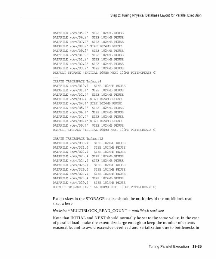
Step 2: Tuning Physical Database Layout for Parallel Execution
DATAFILE /dev/D5.2' SIZE 1024MB REUSEDATAFILE /dev/D6.2' SIZE 1024MB REUSEDATAFILE /dev/D7.2' SIZE 1024MB REUSEDATAFILE /dev/D8.2' SIZE 1024MB REUSEDATAFILE /dev/D9.2' SIZE 1024MB REUSEDATAFILE /dev/D10.2 SIZE 1024MB REUSEDATAFILE /dev/D1.2' SIZE 1024MB REUSEDATAFILE /dev/D2.2' SIZE 1024MB REUSEDATAFILE /dev/D3.2' SIZE 1024MB REUSEDEFAULT STORAGE (INITIAL 100MB NEXT 100MB PCTINCREASE 0)...CREATE TABLESPACE Tsfacts4DATAFILE /dev/D10.4' SIZE 1024MB REUSEDATAFILE /dev/D1.4' SIZE 1024MB REUSEDATAFILE /dev/D2.4' SIZE 1024MB REUSEDATAFILE /dev/D3.4 SIZE 1024MB REUSEDATAFILE /dev/D4.4' SIZE 1024MB REUSEDATAFILE /dev/D5.4' SIZE 1024MB REUSEDATAFILE /dev/D6.4' SIZE 1024MB REUSEDATAFILE /dev/D7.4' SIZE 1024MB REUSEDATAFILE /dev/D8.4' SIZE 1024MB REUSEDATAFILE /dev/D9.4' SIZE 1024MB REUSEDEFAULT STORAGE (INITIAL 100MB NEXT 100MB PCTINCREASE 0)...CREATE TABLESPACE Tsfacts12DATAFILE /dev/D30.4' SIZE 1024MB REUSEDATAFILE /dev/D21.4' SIZE 1024MB REUSEDATAFILE /dev/D22.4' SIZE 1024MB REUSEDATAFILE /dev/D23.4 SIZE 1024MB REUSEDATAFILE /dev/D24.4' SIZE 1024MB REUSEDATAFILE /dev/D25.4' SIZE 1024MB REUSEDATAFILE /dev/D26.4' SIZE 1024MB REUSEDATAFILE /dev/D27.4' SIZE 1024MB REUSEDATAFILE /dev/D28.4' SIZE 1024MB REUSEDATAFILE /dev/D29.4' SIZE 1024MB REUSEDEFAULT STORAGE (INITIAL 100MB NEXT 100MB PCTINCREASE 0)
Extent sizes in the STORAGE clause should be multiples of the multiblock readsize, where
blocksize * MULTIBLOCK_READ_COUNT = multiblock read size
Note that INITIAL and NEXT should normally be set to the same value. In the caseof parallel load, make the extent size large enough to keep the number of extentsreasonable, and to avoid excessive overhead and serialization due to bottlenecks in
Tuning Parallel Execution 19-35
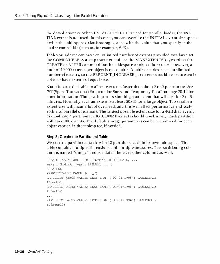
Step 2: Tuning Physical Database Layout for Parallel Execution
the data dictionary. When PARALLEL=TRUE is used for parallel loader, the INI-TIAL extent is not used. In this case you can override the INITIAL extent size speci-fied in the tablespace default storage clause with the value that you specify in theloader control file (such as, for example, 64K).
Tables or indexes can have an unlimited number of extents provided you have setthe COMPATIBLE system parameter and use the MAXEXTENTS keyword on theCREATE or ALTER command for the tablespace or object. In practice, however, alimit of 10,000 extents per object is reasonable. A table or index has an unlimitednumber of extents, so the PERCENT_INCREASE parameter should be set to zero inorder to have extents of equal size.
Note: It is not desirable to allocate extents faster than about 2 or 3 per minute. See"ST (Space Transaction) Enqueue for Sorts and Temporary Data" on page 20-12 formore information. Thus, each process should get an extent that will last for 3 to 5minutes. Normally such an extent is at least 50MB for a large object. Too small anextent size will incur a lot of overhead, and this will affect performance and scal-ability of parallel operations. The largest possible extent size for a 4GB disk evenlydivided into 4 partitions is 1GB. 100MB extents should work nicely. Each partitionwill have 100 extents. The default storage parameters can be customized for eachobject created in the tablespace, if needed.
Step 2: Create the Partitioned TableWe create a partitioned table with 12 partitions, each in its own tablespace. Thetable contains multiple dimensions and multiple measures. The partitioning col-umn is named “dim_2” and is a date. There are other columns as well.
CREATE TABLE fact (dim_1 NUMBER, dim_2 DATE, ...meas_1 NUMBER, meas_2 NUMBER, ... )PARALLEL(PARTITION BY RANGE (dim_2)PARTITION jan95 VALUES LESS THAN ('02-01-1995') TABLESPACETSfacts1PARTITION feb95 VALUES LESS THAN ('03-01-1995') TABLESPACETSfacts2...PARTITION dec95 VALUES LESS THAN ('01-01-1996') TABLESPACETSfacts12);
19-36 Oracle8 Tuning
Step 2: Tuning Physical Database Layout for Parallel Execution
Step 3: Load the Partitions in ParallelThis section describes four alternative approaches to loading partitions in parallel.
The different approaches to loading help you manage the ramifications of the PAR-ALLEL=TRUE keyword of SQL*Loader, which controls whether or not individualpartitions are loaded in parallel. The PARALLEL keyword entails restrictions suchas the following:
■ Indexes cannot be defined.
■ You need to set a small initial extent, because each loader session gets a newextent when it begins, and it doesn’t use any existing space associated with theobject.
■ Space fragmentation issues arise.
However, regardless of the setting of this keyword, if you have one loader processper partition, you are still effectively loading into the table in parallel.
Case 1
In this approach, assume 12 input files that are partitioned in the same way as yourtable. The DBA has 1 input file per partition of the table to be loaded. The DBAstarts 12 SQL*Loader sessions in parallel, entering statements like these:
SQLLDR DATA=jan95.dat DIRECT=TRUE CONTROL=jan95.ctlSQLLDR DATA=feb95.dat DIRECT=TRUE CONTROL=feb95.ctl. . .SQLLDR DATA=dec95.dat DIRECT=TRUE CONTROL=dec95.ctl
Note that the keyword PARALLEL=TRUE is not set. A separate control file per par-tition is necessary because the control file must specify the partition into which theloading should be done. It contains a statement such as:
LOAD INTO fact partition(jan95)
Advantages of this approach are that local indexes are maintained by SQL*Loader.You still get parallel loading, but on a partition level—without the restrictions ofthe PARALLEL keyword.
A disadvantage is that you must partition the input manually.
Tuning Parallel Execution 19-37
Step 2: Tuning Physical Database Layout for Parallel Execution
Case 2
In another common approach, assume an arbitrary number of input files that arenot partitioned in the same way as the table. The DBA can adopt a strategy of per-forming parallel load for each input file individually. Thus if there are 7 input files,the DBA can start 7 SQL*Loader sessions, using statements like the following:
SQLLDR DATA=file1.dat DIRECT=TRUE PARALLEL=TRUE
Oracle will partition the input data so that it goes into the correct partitions. In thiscase all the loader sessions can share the same control file, so there is no need tomention it in the statement.
The keyword PARALLEL=TRUE must be used because each of the 7 loader ses-sions can write into every partition. (In case 1, every loader session would writeinto only 1 partition, because the data was already partitioned outside Oracle.)Hence all the PARALLEL keyword restrictions are in effect.
In this case Oracle attempts to spread the data evenly across all the files in each ofthe 12 tablespaces—however an even spread of data is not guaranteed. Moreover,there could be I/O contention during the load when the loader processes areattempting simultaneously to write to the same device.
Case 3
In Case 3 (illustrated in the example), the DBA wants precise control of the load. Toachieve this the DBA must partition the input data in the same way as the datafilesare partitioned in Oracle.
This example uses 10 processes loading into 30 disks. To accomplish this, the DBAmust split the input into 120 files beforehand. The 10 processes will load the firstpartition in parallel on the first 10 disks, then the second partition in parallel on thesecond 10 disks, and so on through the 12th partition. The DBA runs the followingcommands concurrently as background processes:
SQLLDR DATA=jan95.file1.dat DIRECT=TRUE PARALLEL=TRUE FILE=/dev/D1.1...SQLLDR DATA=jan95.file10.dat DIRECT=TRUE PARALLEL=TRUE FILE=/dev/D10.1WAIT;...SQLLDR DATA=dec95.file1.dat DIRECT=TRUE PARALLEL=TRUE FILE=/dev/D30.4...SQLLDR DATA=dec95.file10.dat DIRECT=TRUE PARALLEL=TRUE FILE=/dev/D29.4
19-38 Oracle8 Tuning
Step 2: Tuning Physical Database Layout for Parallel Execution
For Oracle Parallel Server, divide the loader session evenly among the nodes. Thedatafile being read should always reside on the same node as the loader session.NFS mount of the data file on a remote node is not an optimal approach.
The keyword PARALLEL=TRUE must be used, because multiple loader sessionscan write into the same partition. Hence all the restrictions entailed by the PARAL-LEL keyword are in effect. An advantage of this approach, however, is that it guar-antees that all of the data will be precisely balanced, exactly reflecting yourpartitioning.
Note: Although this example shows parallel load used with partitioned tables, thetwo features can be used independent of one another.
Case 4
For this approach, all of your partitions must be in the same tablespace. You needto have the same number of input files as datafiles in the tablespace, but you do notneed to partition the input the same way in which the table is partitioned.
For example, if all 30 devices were in the same tablespace, then you would arbi-trarily partition your input data into 30 files, then start 30 SQL*Loader sessions inparallel. The statement starting up the first session would be like the following:
SQLLDR DATA=file1.dat DIRECT=TRUE PARALLEL=TRUE FILE=/dev/D1. . .SQLLDR DATA=file30.dat DIRECT=TRUE PARALLEL=TRUE FILE=/dev/D30
The advantage of this approach is that, as in Case 3, you have control over the exactplacement of datafiles, because you use the FILE keyword. However, you are notrequired to partition the input data by value: Oracle does that.
A disadvantage is that this approach requires all the partitions to be in the sametablespace; this minimizes availability.
Tuning Parallel Execution 19-39
Step 2: Tuning Physical Database Layout for Parallel Execution
Setting Up Temporary Tablespaces for Parallel Sort and Hash JoinFor optimal space management performance you can use dedicated temporarytablespaces. As with the TSfacts tablespace, we first add a single datafile and lateradd the remainder in parallel.
CREATE TABLESPACE TStemp TEMPORARY DATAFILE ’/dev/D31’SIZE 4096MB REUSEDEFAULT STORAGE (INITIAL 10MB NEXT 10MB PCTINCREASE 0);
Size of Temporary ExtentsTemporary extents are all the same size, because the server ignores the PCTIN-CREASE and INITIAL settings and only uses the NEXT setting for temporaryextents. This helps to avoid fragmentation.
As a general rule, temporary extents should be smaller than permanent extents,because there are more demands for temporary space, and parallel processes orother operations running concurrently must share the temporary tablespace. Nor-mally, temporary extents should be in the range of 1MB to 10MB. Once you allocatean extent it is yours for the duration of your operation. If you allocate a large extentbut only need to use a small amount of space, the unused space in the extent is tiedup.
At the same time, temporary extents should be large enough that processes do nothave to spend all their time waiting for space. Temporary tablespaces use less over-head than permanent tablespaces when allocating and freeing a new extent. How-ever, obtaining a new temporary extent still requires the overhead of acquiring alatch and searching through the SGA structures, as well as SGA space consumptionfor the sort extent pool. Also, if extents are too small, SMON may take a long timedropping old sort segments when new instances start up.
Operating System Striping of Temporary TablespacesOperating system striping is an alternative technique you can use with temporarytablespaces. Media recovery, however, offers subtle challenges for large temporarytablespaces. It does not make sense to mirror, use RAID, or back up a temporarytablespace. If you lose a disk in an OS striped temporary space, you will probablyhave to drop and recreate the tablespace. This could take several hours for our 120GB example. With Oracle striping, simply remove the bad disk from the tablespace.For example, if /dev/D50 fails, enter:
ALTER DATABASE DATAFILE ‘/dev/D50’ RESIZE 1K;ALTER DATABASE DATAFILE ‘/dev/D50’ OFFLINE;
19-40 Oracle8 Tuning
Step 2: Tuning Physical Database Layout for Parallel Execution
Because the dictionary sees the size as 1K, which is less than the extent size, the badfile will never be accessed. Eventually, you may wish to recreate the tablespace.
Be sure to make your temporary tablespace available for use:
ALTER USER scott TEMPORARY TABLESPACE TStemp;
See Also: For MPP systems, see your platform-specific documentation regardingthe advisability of disabling disk affinity when using operating system striping.
Creating Indexes in ParallelIndexes on the fact table can be partitioned or non-partitioned. Local partitionedindexes provide the simplest administration. The only disadvantage is that a searchof a local non-prefixed index requires searching all index partitions.
The considerations for creating index tablespaces are similar to those for creatingother tablespace. Operating system striping with a small stripe width is often agood choice, but to simplify administration it is best to use a separate tablespace foreach index. If it is a local index you may want to place it into the same tablespace asthe partition to which it corresponds. If each partition is striped over a number ofdisks, the individual index partitions can be rebuilt in parallel for recovery. Alterna-tively, operating system mirroring can be used. For these reasons the NOLOG-GING option of the index creation statement may be attractive for a datawarehouse.
Tablespaces for partitioned indexes should be created in parallel in the same man-ner as tablespaces for partitioned tables.
Partitioned indexes are created in parallel using partition granules, so the maxi-mum degree of parallelism possible is the number of granules. Local index cre-ation has less inherent parallelism than global index creation, and so may run fasterif a higher degree of parallelism is used. The following statement could be used tocreate a local index on the fact table.
CREATE INDEX I on fact(dim_1,dim_2,dim_3) LOCALPARTITION jan95 TABLESPACE Tsidx1,PARTITION feb95 TABLESPACE Tsidx2,...PARALLEL(DEGREE 12) NOLOGGING;
To back up or restore January data, you need only manage tablespace Tsidx1.
See Also: Oracle8 Concepts for a discussion of partitioned indexes.
Tuning Parallel Execution 19-41
Step 2: Tuning Physical Database Layout for Parallel Execution
Additional Considerations for Parallel DML OnlyWhen parallel insert, update, or delete are to be performed on a data warehouse,some additional considerations are needed when designing the physical database.Note that these considerations do not affect parallel query operations. This sectioncovers:
■ Limitation on the Degree of Parallelism
■ Using Local and Global Striping
■ Increasing INITRANS and MAXTRANS
■ Limitation on Available Number of Transaction Free Lists
■ Using Multiple Archivers
■ [NO]LOGGING Option
Limitation on the Degree of ParallelismIf you are performing parallel insert, update, or delete operations, the degree of par-allelism will be equal to or les than the number of partitions in the table.
See Also: "Determining the Degree of Parallelism" on page 19-32
Using Local and Global StripingParallel DML works mostly on partitioned tables. It does not use asynchronous I/Oand may generate a high number of random I/O requests during index mainte-nance of parallel UPDATE and DELETE operations. For local index maintenance,local striping is most efficient in reducing I/O contention, because one server pro-cess will only go to its own set of disks and disk controllers. Local striping alsoincreases availability in the event of one disk failing.
For global index maintenance, (partitioned or non-partitioned), globally stripingthe index across many disks and disk controllers is the best way to distribute thenumber of I/Os.
Increasing INITRANS and MAXTRANSIf you have global indexes, a global index segment and global index blocks will beshared by server processes of the same parallel DML statement. Even if the opera-tions are not performed against the same row, the server processes may share thesame index blocks. Each server transaction needs one transaction entry in the indexblock header before it can make changes to a block. Therefore, in the CREATEINDEX or ALTER INDEX statements, you should set INITRANS (the initial num-
19-42 Oracle8 Tuning
Step 2: Tuning Physical Database Layout for Parallel Execution
ber of transactions allocated within each data block) to a large value, such as themaximum degree of parallelism against this index. Leave MAXTRANS, the maxi-mum number of concurrent transactions that can update a data block, at its defaultvalue, which is the maximum your system can support (not to exceed 255).
If you run degree 10 parallelism against a table with a global index, all 10 serverprocesses might attempt to change the same global index block. For this reason youmust set MAXTRANS to at least 10 so that all the server processes can make thechange at the same time. If MAXTRANS is not large enough, the parallel DMLoperation will fail.
Limitation on Available Number of Transaction Free ListsOnce a segment has been created, the number of process and transaction free lists isfixed and cannot be altered. If you specify a large number of process free lists in thesegment header, you may find that this limits the number of transaction free liststhat are available. You can abate this limitation the next time you recreate the seg-ment header by decreasing the number of process free lists; this will leave moreroom for transaction free lists in the segment header.
For UPDATE and DELETE operations, each server process may require its owntransaction free list. The parallel DML degree of parallelism is thus effectively lim-ited by the smallest number of transaction free lists available on any of the globalindexes which the DML statement must maintain. For example, if you have twoglobal indexes, one with 50 transaction free lists and one with 30 transaction freelists, the degree of parallelism is limited to 30.
Note that the FREELISTS parameter of the STORAGE clause is used to set the num-ber of process free lists. By default, no process free lists are created.
The default number of transaction free lists depends on the block size. For example,if the number of process free lists is not set explicitly, a 4K block has about 80 trans-action free lists by default. The minimum number of transaction free lists is 25.
See Also: Oracle8 Parallel Server Concepts & Administration for information abouttransaction free lists.
Using Multiple ArchiversParallel DDL and parallel DML operations may generate a large amount of redologs. A single ARCH process to archive these redo logs might not be able to keepup. To avoid this problem, you can spawn multiple archiver processes. This can bedone manually or by using a job queue.
Tuning Parallel Execution 19-43
Step 2: Tuning Physical Database Layout for Parallel Execution
Database Writer Process (DBWn) WorkloadParallel DML operations dirty a large number of data, index, and undo blocks inthe buffer cache during a short period of time. If you see a high number of“free_buffer_waits” in the V$SYSSTAT view, tune the DBWn process(es).
See Also: "Tuning the Redo Log Buffer" on page 14-7
[NO]LOGGING OptionThe [NO]LOGGING option applies to tables, partitions, tablespaces, and indexes.Virtually no log is generated for certain operations (such as direct-load INSERT) ifthe NOLOGGING option is used. The NOLOGGING attribute is not specified atthe INSERT statement level, but is instead specified when using the ALTER or CRE-ATE command for the table, partition, index, or tablespace.
When a table or index has NOLOGGING set, neither parallel nor serial direct-loadINSERT operations generate undo or redo logs. Processes running with theNOLOGGING option set run faster because no redo is generated. However, after aNOLOGGING operation against a table, partition, or index, if a media failureoccurs before a backup is taken, then all tables, partitions, and indexes that havebeen modified may be corrupted.
Note: Direct-load INSERT operations (except for dictionary updates) never gener-ate undo logs. The NOLOGGING attribute does not affect undo, but only redo. Tobe precise, NOLOGGING allows the direct-load INSERT operation to generate anegligible amount of redo (range-invalidation redo, as opposed to full image redo).
For backward compatibility, [UN]RECOVERABLE is still supported as an alternatekeyword with the CREATE TABLE statement in Oracle8 Server, release 8.0. Thisalternate keyword may not be supported, however, in future releases.
AT the tablespace level, the logging clause specifies the default logging attribute forall tables, indexes, and partitions created in the tablespace. When an existingtablespace logging attribute is changed by the ALTER TABLESPACE statement,then all tables, indexes, and partitions created after the ALTER statement will havethe new logging attribute; existing ones will not change their logging attributes.The tablespace level logging attribute can be overridden by the specifications at thetable, index, or partition level).
The default logging attribute is LOGGING. However, if you have put the databaseis in NOARCHIVELOG mode (by issuing ALTER DATABASE NOARCHIVELOG),then all operations that can be done without logging will not generate logs, regard-less of the specified logging attribute.
See Also: Oracle8 SQL Reference
19-44 Oracle8 Tuning
Step 3: Analyzing Data
Step 3: Analyzing DataAfter the data is loaded and indexed, analyze it. It is very important to analyze thedata after any DDL changes or major DML changes. The ANALYZE commanddoes not execute in parallel against a single table or partition. However, many dif-ferent partitions of a partitioned table can be analyzed in parallel. Use the storedprocedure DBMS_UTILITY.ANALYZE_PART_OBJECT to submit jobs to a jobqueue in order to analyze a partitioned table in parallel.
ANALYZE must be run twice in the following sequence to gather table and indexstatistics, and to create histograms. (The second ANALYZE statement creates histo-grams on columns.)
ANALYZE TABLE xyz ESTIMATE STATISTICS;ANALYZE TABLE xyz ESTIMATE STATISTICS FOR ALL COLUMNS;
ANALYZE TABLE gathers statistics at the table level (for example, the number ofrows and blocks), and for all dependent objects, such as columns and indexes. Ifrun in the reverse sequence, the table-only ANALYZE will destroy the histogramsbuilt by the column-only ANALYZE.
An ESTIMATE of statistics produces accurate histograms for small tables only.Once the table is more than a few thousand rows, accurate histograms can only beensured if more than the default number of rows is sampled. The sample size youchoose depends on several factors: the objects to be analyzed (table, indexes, col-umns); the nature of the data (skewed or not); whether you are building histo-grams; as well as the performance you expect. The sample size for analyzing anindex or a table need not be big; 1 percent is more than enough for tables contain-ing more than 2000 rows.
Queries with many joins are quite sensitive to the accuracy of the statistics. Use theCOMPUTE option of the ANALYZE command if possible (it may take quite sometime and a large amount of temporary space). If you must use the ESTIMATEoption, sample as large a percentage as possible (for example, 10%). If you use toohigh a sample size for ESTIMATE, however, this process may require practicallythe same execution time as COMPUTE. A good rule of thumb, in this case, is not tochoose a percentage which causes you to access every block in the system. Forexample, if you have 20 blocks, and each block has 1000 rows, estimating 20% willcause you to touch every block. You may as well have computed the statistics!
Use histograms for data that is not uniformly distributed. Note that a great deal ofdata falls into this classification.
When you analyze a table, Oracle also analyzes all the different objects that aredefined on that table: the table as well as its columns and indexes. Note that you
Tuning Parallel Execution 19-45
Step 3: Analyzing Data
can use the ANALYZE INDEX statement to analyze the index separately. You maywish to do this when you add a new index to the table; it enables you to specify adifferent sample size. You can analyze all partitions of facts (including indexes) inparallel in one of two ways:
■ Execute the following command. Make sure that job queues are enabled beforethe command is executed.
EXECUTE DBMS_UTILITY.ANALYZE_PART_OBJECT(OBJECT_NAME=>'facts',COMMAND_TYPE=>'C');
■ Concurrently, you can issue multiple ANALYZE commands concurrently.
It is worthwhile computing or estimating with a larger sample size the indexed col-umns, rather than the measure data. The measure data is not used as much: most ofthe predicates and critical optimizer information comes from the dimensions. ADBA should know which columns are the most frequently used in predicates.
For example, you might analyze the data in two passes. In the first pass you couldobtain some statistics by analyzing 1% of the data. Run the following command tosubmit analysis commands to the job queues:
EXECUTE DBMS_UTILITY.ANALYZE_PART_OBJECT(OBJECT_NAME=>'facts',COMMAND_TYPE=>'E',SAMPLE_CLAUSE=>'SAMPLE 1 PERCENT');
In a second pass, you could refine statistics for the indexed columns and the index(but not the non-indexed columns):
EXECUTE DBMS_UTILITY.ANALYZE_PART_OBJECT(OBJECT_NAME=>'facts',COMMAND_TYPE=>'C',COMMAND_OPT=>'FOR ALL INDEXEDCOLUMNS SIZE 1');EXECUTE DBMS_UTILITY.ANALYZE_PART_OBJECT(OBJECT_NAME=>'facts',COMMAND_TYPE=>'C',COMMAND_OPT=>'FOR ALL INDEXES'):
The result will be a faster plan because you have collected accurate statistics on themost sensitive columns. You are spending more resources to get good statistics onhigh-value columns (indexes and join columns), and getting baseline statistics forthe rest of the data.
Note: Cost-based optimization is always used with parallel execution and with par-titioned tables. You must therefore analyze partitioned tables or tables used withparallel query.
19-46 Oracle8 Tuning
Understanding Parallel Execution Performance
20
Understanding Parallel ExecutionPerformance Issues
This chapter provides a conceptual explanation of parallel execution performanceissues, and additional performance techniques.
■ Understanding Parallel Execution Performance Issues
■ Parallel Execution Tuning Techniques
See Also: Oracle8 Concepts, for basic principles of parallel execution.
See your operating system-specific Oracle documentation for more informationabout tuning while using parallel execution.
Issues 20-1
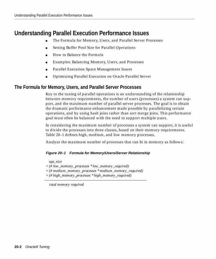
Understanding Parallel Execution Performance Issues
Understanding Parallel Execution Performance Issues■ The Formula for Memory, Users, and Parallel Server Processes
■ Setting Buffer Pool Size for Parallel Operations
■ How to Balance the Formula
■ Examples: Balancing Memory, Users, and Processes
■ Parallel Execution Space Management Issues
■ Optimizing Parallel Execution on Oracle Parallel Server
The Formula for Memory, Users, and Parallel Server ProcessesKey to the tuning of parallel operations is an understanding of the relationshipbetween memory requirements, the number of users (processes) a system can sup-port, and the maximum number of parallel server processes. The goal is to obtainthe dramatic performance enhancement made possible by parallelizing certainoperations, and by using hash joins rather than sort merge joins. This performancegoal must often be balanced with the need to support multiple users.
In considering the maximum number of processes a system can support, it is usefulto divide the processes into three classes, based on their memory requirements.Table 20–1 defines high, medium, and low memory processes.
Analyze the maximum number of processes that can fit in memory as follows:
Figure 20–1 Formula for Memory/Users/Server Relationship
sga_size+ (# low_memory_processes * low_memory_required)+ (# medium_memory_processes * medium_memory_required)+ (# high_memory_processes * high_memory_required)
total memory required
20-2 Oracle8 Tuning
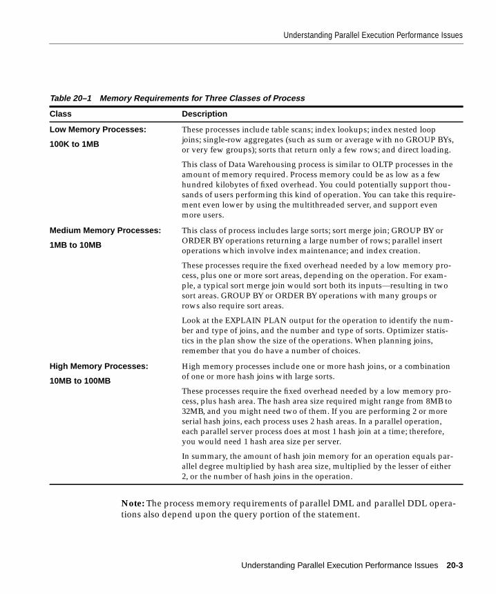
Understanding Parallel Execution Performance Issues
Note: The process memory requirements of parallel DML and parallel DDL opera-tions also depend upon the query portion of the statement.
Table 20–1 Memory Requirements for Three Classes of Process
Class Description
Low Memory Processes:
100K to 1MB
These processes include table scans; index lookups; index nested loopjoins; single-row aggregates (such as sum or average with no GROUP BYs,or very few groups); sorts that return only a few rows; and direct loading.
This class of Data Warehousing process is similar to OLTP processes in theamount of memory required. Process memory could be as low as a fewhundred kilobytes of fixed overhead. You could potentially support thou-sands of users performing this kind of operation. You can take this require-ment even lower by using the multithreaded server, and support evenmore users.
Medium Memory Processes:
1MB to 10MB
This class of process includes large sorts; sort merge join; GROUP BY orORDER BY operations returning a large number of rows; parallel insertoperations which involve index maintenance; and index creation.
These processes require the fixed overhead needed by a low memory pro-cess, plus one or more sort areas, depending on the operation. For exam-ple, a typical sort merge join would sort both its inputs—resulting in twosort areas. GROUP BY or ORDER BY operations with many groups orrows also require sort areas.
Look at the EXPLAIN PLAN output for the operation to identify the num-ber and type of joins, and the number and type of sorts. Optimizer statis-tics in the plan show the size of the operations. When planning joins,remember that you do have a number of choices.
High Memory Processes:
10MB to 100MB
High memory processes include one or more hash joins, or a combinationof one or more hash joins with large sorts.
These processes require the fixed overhead needed by a low memory pro-cess, plus hash area. The hash area size required might range from 8MB to32MB, and you might need two of them. If you are performing 2 or moreserial hash joins, each process uses 2 hash areas. In a parallel operation,each parallel server process does at most 1 hash join at a time; therefore,you would need 1 hash area size per server.
In summary, the amount of hash join memory for an operation equals par-allel degree multiplied by hash area size, multiplied by the lesser of either2, or the number of hash joins in the operation.
Understanding Parallel Execution Performance Issues 20-3
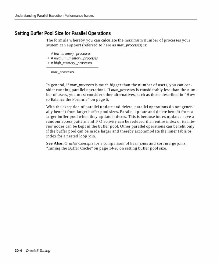
Understanding Parallel Execution Performance Issues
Setting Buffer Pool Size for Parallel OperationsThe formula whereby you can calculate the maximum number of processes yoursystem can support (referred to here as max_processes) is:
In general, if max_processes is much bigger than the number of users, you can con-sider running parallel operations. If max_processes is considerably less than the num-ber of users, you must consider other alternatives, such as those described in “Howto Balance the Formula” on page 5.
With the exception of parallel update and delete, parallel operations do not gener-ally benefit from larger buffer pool sizes. Parallel update and delete benefit from alarger buffer pool when they update indexes. This is because index updates have arandom access pattern and I/O activity can be reduced if an entire index or its inte-rior nodes can be kept in the buffer pool. Other parallel operations can benefit onlyif the buffer pool can be made larger and thereby accommodate the inner table orindex for a nested loop join.
See Also: Oracle8 Concepts for a comparison of hash joins and sort merge joins."Tuning the Buffer Cache" on page 14-26 on setting buffer pool size.
# low_memory_processes+ # medium_memory_processes+ # high_memory_processes
max_processes
20-4 Oracle8 Tuning
Understanding Parallel Execution Performance Issues
How to Balance the FormulaUse the following techniques to balance the memory/users/server formula givenin Figure 20–1:
■ Oversubscribe, with Attention to Paging
■ Reduce the Number of Memory-Intensive Processes
■ Decrease Data Warehousing Memory per Process
■ Decrease Parallelism for Multiple Users
Oversubscribe, with Attention to PagingYou can permit the potential workload to exceed the limits recommended in the for-mula. Total memory required, minus the SGA size, can be multiplied by a factor of1.2, to allow for 20% oversubscription. Thus, if you have 1G of memory, you mightbe able to support 1.2G of demand: the other 20% could be handled by the pagingsystem.
You must, however, verify that a particular degree of oversubscription will be via-ble on your system by monitoring the paging rate and making sure you are notspending more than a very small percent of the time waiting for the paging sub-system. Your system may perform acceptably even if oversubscribed by 60%, if onaverage not all of the processes are performing hash joins concurrently. Usersmight then try to use more than the available memory, so you must monitor pagingactivity in such a situation. If paging goes up dramatically, consider another alterna-tive.
On average, no more than 5% of the time should be spent simply waiting in theoperating system on page faults. More than 5% wait time indicates an I/O boundpaging subsystem. Use your operating system monitor to check wait time: The sumof time waiting and time running equals 100%. If you are running close to 100%CPU, then you are not waiting. If you are waiting, it should not be on account ofpaging.
If wait time for paging devices exceeds 5%, it is a strong indication that you mustreduce memory requirements in one of these ways:
■ Reducing the memory required for each class of process
■ Reducing the number of processes in memory-intensive classes
■ Adding memory
If the wait time indicates an I/O bottleneck in the paging subsystem, you couldresolve this by striping.
Understanding Parallel Execution Performance Issues 20-5
Understanding Parallel Execution Performance Issues
Reduce the Number of Memory-Intensive ProcessesAdjusting the Degree of Parallelism. You can adjust not only the number of opera-tions that run in parallel, but also the degree of parallelism with which operationsrun. To do this, issue an ALTER TABLE statement with a PARALLEL clause, or usea hint. See the Oracle8 SQL Reference for more information.
You can limit the parallel pool by reducing the value ofPARALLEL_MAX_SERVERS. Doing so places a system-level limit on the totalamount of parallelism, and is easy to administer. More processes are then forced torun in serial mode.
Scheduling Parallel Jobs. Queueing jobs is another way to reduce the number ofprocesses but not reduce parallelism. Rather than reducing parallelism for all opera-tions, you may be able to schedule large parallel batch jobs to run with full parallel-ism one at a time, rather than concurrently. Queries at the head of the queue wouldhave a fast response time, those at the end of the queue would have a slowresponse time. However, this method entails a certain amount of administrativeoverhead.
Decrease Data Warehousing Memory per ProcessNote: The following discussion focuses upon the relationship ofHASH_AREA_SIZE to memory, but all the same considerations apply toSORT_AREA_SIZE. The lower bound of SORT_AREA_SIZE, however, is not as crit-ical as the 8MB recommended minimum HASH_AREA_SIZE.
If every operation performs a hash join and a sort, the high memory requirementlimits the number of processes you can have. To allow more users to run concur-rently you may need to reduce the DSS process memory.
Moving Processes from High to Medium Memory Requirements. You can move aprocess from the high-memory to the medium-memory class by changing fromhash join to merge join. You can use initialization parameters to limit availablememory and thus force the optimizer to stay within certain bounds.
To do this, you can reduce HASH_AREA_SIZE to well below the recommendedminimum (for example, to 1 or 2MB). Then you can let the optimizer choose sortmerge join more often (as opposed to telling the optimizer never to use hash joins).In this way, hash join can still be used for small tables: the optimizer has a memorybudget within which it can make decisions about which join method to use. Alter-natively, you can use hints to force only certain queries (those whose response timeis not critical) to use sort-merge joins rather than hash joins.
20-6 Oracle8 Tuning
Understanding Parallel Execution Performance Issues
Remember that the recommended parameter values provide the best responsetime. If you severely limit these values you may see a significant effect on responsetime.
Moving Processes from High or Medium Memory Requirements to Low Mem-ory Requirements. If you need to support thousands of users, you must createaccess paths such that operations do not touch much data.
■ Decrease the demand for index joins by creating indexes and/or summarytables.
■ Decrease the demand for GROUP BY sorting by creating summary tables andencouraging users and applications to reference summaries rather thandetailed data.
■ Decrease the demand for ORDER BY sorts by creating indexes on frequentlysorted columns.
Decrease Parallelism for Multiple UsersIn general there is a trade-off between parallelism for fast single-user response timeand efficient use of resources for multiple users. For example, a system with 2G ofmemory and a HASH_AREA_SIZE of 32MB can support about 60 parallel serverprocesses. A 10 CPU machine can support up to 3 concurrent parallel operations (2* 10 * 3 = 60). In order to support 12 concurrent parallel operations, you could over-ride the default parallelism (reduce it); decrease HASH_AREA_SIZE; buy morememory, or use some combination of these three strategies. Thus you could ALTERTABLE t PARALLEL (DEGREE 5) for all parallel tables t, set HASH_AREA_SIZE to16MB, and increase PARALLEL_MAX_SERVERS to 120. By reducing the memoryof each parallel server by a factor of 2, and reducing the parallelism of a single oper-ation by a factor of 2, the system can accommodate 2 * 2 = 4 times more concurrentparallel operations.
The penalty for taking such an approach is that when a single operation happens tobe running, the system will use just half the CPU resource of the 10 CPU machine.The other half will be idle until another operation is started.
To determine whether your system is being fully utilized, you can use one of thegraphical system monitors available on most operating systems. These monitorsoften give you a better idea of CPU utilization and system performance than moni-toring the execution time of an operation. Consult your operating system documen-tation to determine whether your system supports graphical system monitors.
Understanding Parallel Execution Performance Issues 20-7
Understanding Parallel Execution Performance Issues
Examples: Balancing Memory, Users, and ProcessesThe examples in this section show how to evaluate the relationship between mem-ory, users, and parallel server processes, and balance the formula given inFigure 20–1. They show concretely how you might adjust your system workload soas to accommodate the necessary number of processes and users.
Example 1Assume that your system has 1G of memory, the degree of parallelism is 10, andthat your users perform 2 hash joins with 3 or more tables. If you need 300MB forthe SGA, that leaves 700MB to accommodate processes. If you allow a generoushash area size (32MB) for best performance, then your system can support:
1 parallel operation (32MB * 10 * 2 = 640MB)1 serial operation (32MB * 2 = 64MB)
This makes a total of 704MB. (Note that the memory is not significantly oversub-scribed.)
Remember that every parallel, hash, or sort merge join operation takes a number ofparallel server processes equal to twice the degree of parallelism (utilizing 2 serversets), and often each individual process of a parallel operation uses a lot of mem-ory. Thus you can support many more users by having them run serially, or by hav-ing them run with less parallelism.
To service more users, you can drastically reduce hash area size to 2MB. You maythen find that the optimizer switches some operations to sort merge join. This con-figuration can support 17 parallel operations, or 170 serial operations, but responsetimes may be significantly higher than if you were using hash joins.
Notice the trade-off above: by reducing memory per process by a factor of 16, youcan increase the number of concurrent users by a factor of 16. Thus the amount ofphysical memory on the machine imposes another limit on total number of paralleloperations you can run involving hash joins and sorts.
20-8 Oracle8 Tuning
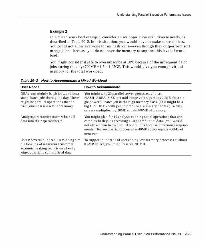
Understanding Parallel Execution Performance Issues
Example 2In a mixed workload example, consider a user population with diverse needs, asdescribed in Table 20–2. In this situation, you would have to make some choices.You could not allow everyone to run hash joins—even though they outperform sortmerge joins—because you do not have the memory to support this level of work-load.
You might consider it safe to oversubscribe at 50% because of the infrequent batchjobs during the day: 700MB * 1.5 = 1.05GB. This would give you enough virtualmemory for the total workload.
Table 20–2 How to Accommodate a Mixed Workload
User Needs How to Accommodate
DBA: runs nightly batch jobs, and occa-sional batch jobs during the day. Thesemight be parallel operations that dohash joins that use a lot of memory.
You might take 20 parallel server processes, and setHASH_AREA_SIZE to a mid-range value, perhaps 20MB, for a sin-gle powerful batch job in the high memory class. (This might be abig GROUP BY with join to produce a summary of data.) Twentyservers multiplied by 20MB equals 400MB of memory.
Analysts: interactive users who pulldata into their spreadsheets
You might plan for 10 analysts running serial operations that usecomplex hash joins accessing a large amount of data. (You wouldnot allow them to do parallel operations because of memory require-ments.) Ten such serial processes at 40MB apiece equals 400MB ofmemory.
Users: Several hundred users doing sim-ple lookups of individual customeraccounts, making reports on alreadyjoined, partially summarized data
To support hundreds of users doing low memory processes at about0.5MB apiece, you might reserve 200MB.
Understanding Parallel Execution Performance Issues 20-9
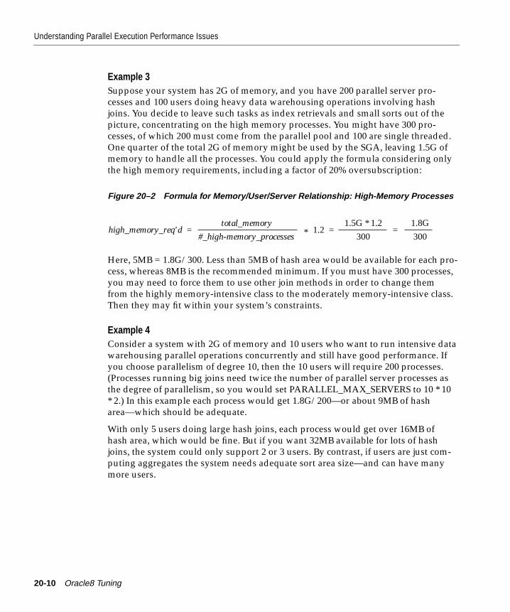
Understanding Parallel Execution Performance Issues
Example 3Suppose your system has 2G of memory, and you have 200 parallel server pro-cesses and 100 users doing heavy data warehousing operations involving hashjoins. You decide to leave such tasks as index retrievals and small sorts out of thepicture, concentrating on the high memory processes. You might have 300 pro-cesses, of which 200 must come from the parallel pool and 100 are single threaded.One quarter of the total 2G of memory might be used by the SGA, leaving 1.5G ofmemory to handle all the processes. You could apply the formula considering onlythe high memory requirements, including a factor of 20% oversubscription:
Figure 20–2 Formula for Memory/User/Server Relationship: High-Memory Processes
Here, 5MB = 1.8G/300. Less than 5MB of hash area would be available for each pro-cess, whereas 8MB is the recommended minimum. If you must have 300 processes,you may need to force them to use other join methods in order to change themfrom the highly memory-intensive class to the moderately memory-intensive class.Then they may fit within your system’s constraints.
Example 4Consider a system with 2G of memory and 10 users who want to run intensive datawarehousing parallel operations concurrently and still have good performance. Ifyou choose parallelism of degree 10, then the 10 users will require 200 processes.(Processes running big joins need twice the number of parallel server processes asthe degree of parallelism, so you would set PARALLEL_MAX_SERVERS to 10 * 10* 2.) In this example each process would get 1.8G/200—or about 9MB of hasharea—which should be adequate.
With only 5 users doing large hash joins, each process would get over 16MB ofhash area, which would be fine. But if you want 32MB available for lots of hashjoins, the system could only support 2 or 3 users. By contrast, if users are just com-puting aggregates the system needs adequate sort area size—and can have manymore users.
high_memory_req'd = 1.2 = =*total_memory
#_high-memory_processes
1.5G * 1.2300
1.8G300
20-10 Oracle8 Tuning
Understanding Parallel Execution Performance Issues
Example 5If a system with 2G of memory needs to support 1000 users, all of them running bigoperations, you must evaluate the situation carefully. Here, the per-user memorybudget is only 1.8MB (that is, 1.8G divided by 1,000). Since this figure is at the lowend of the medium memory process class, you must rule out parallel operations,which use even more resources. You must also rule out big hash joins. Each sequen-tial process could require up to 2 hash areas plus the sort area, so you would haveto set HASH_AREA_SIZE to the same value as SORT_AREA_SIZE, which wouldbe 600K (1.8MB/3). Such a small hash area size is likely to be ineffective, so youmay opt to disable hash joins altogether.
Given the organization’s resources and business needs, is it reasonable for you toupgrade your system’s memory? If memory upgrade is not an option, then youmust change your expectations. To adjust the balance you might:
■ Accept the fact that the system will actually support a limited number of usersdoing big hash joins.
■ Expect to support the 1000 users doing index lookups and joins that do notrequire large amounts of memory. Sort merge joins require less memory, butthroughput will go down because they are not as efficient as hash joins.
■ Give the users access to summary tables, rather than to the whole database.
■ Classify users into different groups, and give some groups more memory thanothers. Instead of all users doing sorts with a small sort area, you could have afew users doing high-memory hash joins, while most users use summary tablesor do low-memory index joins. (You could accomplish this by forcing users ineach group to use hints in their queries such that operations are performed in aparticular way.)
Understanding Parallel Execution Performance Issues 20-11
Understanding Parallel Execution Performance Issues
Parallel Execution Space Management IssuesThis section describes space management issues that come into play when usingparallel execution.
■ ST (Space Transaction) Enqueue for Sorts and Temporary Data
■ External Fragmentation
These issues become particularly important for parallel operation running on a par-allel server, the more nodes involved, the more tuning becomes critical.
ST (Space Transaction) Enqueue for Sorts and Temporary DataEvery space management transaction in the database (such as creation of tempo-rary segments in PARALLEL CREATE TABLE, or parallel direct-load inserts of non-partitioned tables) is controlled by a single ST enqueue. A high transaction rate(more than 2 or 3 per minute) on the ST enqueue may result in poor scalability onOracle Parallel Server systems with many nodes, or a timeout waiting for spacemanagement resources.
Try to minimize the number of space management transactions, in particular:
■ the number of sort space management transactions
■ the creation and removal of objects
■ transactions caused by fragmentation in a tablespace.
Use dedicated temporary tablespaces to optimize space management for sorts. Thisis particularly beneficial on a parallel server. You can monitor this usingV$SORT_SEGMENT.
Set INITIAL and NEXT extent size to a value in the range of 1MB to 10MB. Pro-cesses may use temporary space at a rate of up to 1MB per second. Do not acceptthe default value of 40K for next extent size, because this will result in manyrequests for space per second.
If you are unable to allocate extents for various reasons, you can recoalesce thespace by using the ALTER TABLESPACE ... COALESCE SPACE command. Thisshould be done on a regular basis for temporary tablespaces in particular.
See Also: "Setting Up Temporary Tablespaces for Parallel Sort and Hash Join" onpage 19-40
20-12 Oracle8 Tuning

Understanding Parallel Execution Performance Issues
External FragmentationExternal fragmentation is a concern for parallel load, direct-load insert, and PARAL-LEL CREATE TABLE ... AS SELECT. Memory tends to become fragmented asextents are allocated and data is inserted and deleted. This may result in a fairamount of free space that is unusable because it consists of small, non-contiguouschunks of memory. To reduce external fragmentation on partitioned tables, set allextents to the same size. Set MINEXTENTS to the same value as NEXT, whichshould be equal to INITIAL; set PERCENT_INCREASE to zero. The system canhandle this well with a few thousand extents per object, so you can set MAXEX-TENTS to a few thousand. For tables that are not partitioned, the initial extentshould be small.
Optimizing Parallel Execution on Oracle Parallel ServerThis section describe several aspects of parallel execution on Oracle Parallel Server.
Lock AllocationThis section provides parallel execution tuning guidelines for optimal lock manage-ment on Oracle Parallel Server.
To optimize parallel execution on Oracle Parallel Server, you need to correctly setGC_FILES_TO_LOCKS. On Oracle Parallel Server a certain number of parallelcache management (PCM) locks are assigned to each data file. Data block address(DBA) locking in its default behavior assigns one lock to each block. During a fulltable scan a PCM lock must then be acquired for each block read into the scan. Tospeed up full table scans, you have three possibilities:
■ For data files containing truly read-only data, set the tablespace to read only.Then there will be no PCM locking at all.
■ Alternatively, for data that is mostly read-only, assign very few hashed PCMlocks (for example, 2 shared locks) to each data file. Then these will be the onlylocks you have to acquire when you read the data.
■ If you want DBA or fine-grain locking, group together the blocks controlled byeach lock, using the ! option. This has advantages over default DBA lockingbecause with the default, you would need to acquire a million locks in order toread 1 million blocks. When you group the blocks you reduce the number oflocks allocated by the grouping factor. Thus a grouping of !10 would mean thatyou would only have to acquire one tenth as many PCM locks as with thedefault. Performance improves due to the dramatically reduced amount of lockallocation. As a rule of thumb, performance with a grouping of !10 might becomparable to the speed of hashed locking.
Understanding Parallel Execution Performance Issues 20-13
Understanding Parallel Execution Performance Issues
To speed up parallel DML operations, consider using hashed locking ratherthan DBA locking. A parallel server process works on non-overlapping parti-tions; it is recommended that partitions not share files. You can thus reduce thenumber of lock operations by having only 1 hashed lock per file. Since the par-allel server process only works on non-overlapping files, there will be no lockpings.
The following guidelines impact memory usage, and thus indirectly affect perfor-mance:
■ Never allocate PCM locks for datafiles of temporary tablespaces.
■ Never allocate PCM locks for datafiles that contain only rollback segments.These are protected by GC_ROLLBACK_LOCKS andGC_ROLLBACK_SEGMENTS.
■ Allocate specific PCM locks for the SYSTEM tablespace. This practice ensuresthat data dictionary activity such as space management never interferes withthe data tablespaces at a cache management level (error 1575).
For example, on a read-only database with a data warehousing application’squery-only workload, you might create 500 PCM locks on the SYSTEMtablespace in file 1, then create 50 more locks to be shared for all the data in theother files. Space management work will then never interfere with the rest ofthe database.
See Also: Oracle8 Parallel Server Concepts & Administration for a thorough discussionof PCM locks and locking parameters.
Allocation of Processes and InstancesParallel execution assigns each instance a unique number, which is determined bythe INSTANCE_NUMBER initialization parameter. The instance number regulatesthe order of instance startup.
Note: For Oracle Parallel Server, the PARALLEL_INSTANCE_GROUP parameterdetermines what instance group will be used for a particular operation. For moreinformation, see Oracle8 Parallel Server Concepts & Administration.
Oracle computes a target degree of parallelism by examining the maximum of thedegree for each table and other factors, before run time. At run time, a parallel oper-ation is executed sequentially if insufficient parallel server processes are available.PARALLEL_MIN_PERCENT sets the minimum percentage of the target number ofparallel server processes that must be available in order for the operation to run inparallel. When PARALLEL_MIN_PERCENT is set to n, an error message is sent if n
20-14 Oracle8 Tuning
Understanding Parallel Execution Performance Issues
percent parallel server processes are not available. If no parallel server processesare available, a parallel operation is executed sequentially.
Load Balancing for Multiple Concurrent Parallel OperationsLoad balancing is the distribution of parallel server processes to achieve even CPUand memory utilization, and to minimize remote I/O and communication betweennodes.
When multiple concurrent operations are running on a single node, load balancingis done by the operating system. For example, if there are 10 CPUs and 5 parallelserver processes, the operating system distributes the 5 processes among the CPUs.If a second node is added, the operating system still distributes the workload.
For a parallel server, however, no single operating system performs the load balanc-ing: instead, parallel execution performs this function.
If an operation requests more than one instance, allocation priorities involve tablecaching and disk affinity.
Thus, if there are 5 parallel server processes, it is advantageous for them to run onas many nodes as possible.
In Oracle Server release 8.0, allocation of processes and instances is based oninstance groups. With instance groups a parallel server system will be partitionedinto disjoint logical subsystems. Parallel resources will be allocated out of a particu-lar instance group only if the parallel coordinator is part of the group. Thisapproach supports application and data partitioning.
See Also: Oracle8 Parallel Server Concepts & Administration for more informationabout instance groups.
Disk AffinitySome Oracle Parallel Server platforms use disk affinity. Without disk affinity, Ora-cle tries to balance the allocation evenly across instances; with disk affinity, Oracletries to allocate parallel server processes for parallel table scans on the instancesthat are closest to the requested data. Disk affinity minimizes data shipping andinternode communication on a shared nothing architecture. It can significantlyincrease parallel operation throughput and decrease response time.
Disk affinity is used for parallel table scans, parallel temporary tablespace alloca-tion, parallel DML, and parallel index scan. It is not used for parallel table creationor parallel index creation. Access to temporary tablespaces preferentially uses localdatafiles. It guarantees optimal space management extent allocation. Disks stripedby the operating system are treated by disk affinity as a single unit.
Understanding Parallel Execution Performance Issues 20-15
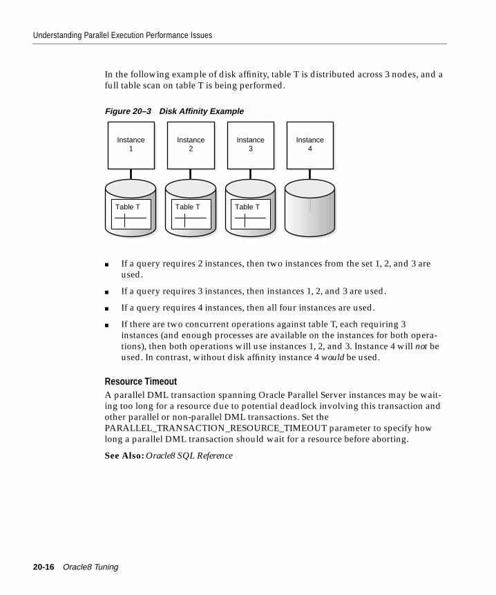
Understanding Parallel Execution Performance Issues
In the following example of disk affinity, table T is distributed across 3 nodes, and afull table scan on table T is being performed.
Figure 20–3 Disk Affinity Example
■ If a query requires 2 instances, then two instances from the set 1, 2, and 3 areused.
■ If a query requires 3 instances, then instances 1, 2, and 3 are used.
■ If a query requires 4 instances, then all four instances are used.
■ If there are two concurrent operations against table T, each requiring 3instances (and enough processes are available on the instances for both opera-tions), then both operations will use instances 1, 2, and 3. Instance 4 will not beused. In contrast, without disk affinity instance 4 would be used.
Resource TimeoutA parallel DML transaction spanning Oracle Parallel Server instances may be wait-ing too long for a resource due to potential deadlock involving this transaction andother parallel or non-parallel DML transactions. Set thePARALLEL_TRANSACTION_RESOURCE_TIMEOUT parameter to specify howlong a parallel DML transaction should wait for a resource before aborting.
See Also: Oracle8 SQL Reference
Instance1
Table T
Instance2
Table T
Instance3
Table T
Instance4
20-16 Oracle8 Tuning
Parallel Execution Tuning Techniques
Parallel Execution Tuning TechniquesThis section describes performance techniques for parallel operations.
■ Overriding the Default Degree of Parallelism
■ Rewriting SQL Statements
■ Creating and Populating Tables in Parallel
■ Creating Indexes in Parallel
■ Refreshing Tables in Parallel
■ Using Hints with Cost Based Optimization
■ Tuning Parallel Insert Performance
Overriding the Default Degree of ParallelismThe default degree of parallelism is appropriate for reducing response time whileguaranteeing use of CPU and I/O resources for any parallel operations. If an opera-tion is I/O bound, you should consider increasing the default degree of parallel-ism. If it is memory bound, or several concurrent parallel operations are running,consider decreasing the default degree.
Oracle uses the default degree of parallelism for tables that have PARALLEL attrib-uted to them in the data dictionary, or when the PARALLEL hint is specified. If atable does not have parallelism attributed to it, or has NOPARALLEL (the default)attributed to it, then that table is never scanned in parallel—regardless of thedefault degree of parallelism that would be indicated by the number of CPUs,instances, and devices storing that table.
Use the following guidelines when adjusting the degree of parallelism:
■ You can adjust the degree of parallelism either by using ALTER TABLE or byusing hints.
■ To increase the number of concurrent parallel operations, reduce the degree ofparallelism.
■ For I/O-bound parallel operations, first spread the data over more disks thanthere are CPUs. Then, increase parallelism in stages. Stop when the querybecomes CPU bound.
For example, assume a parallel indexed nested loop join is I/O bound perform-ing the index lookups, with #CPUs=10 and #disks=36. The default degree of par-allelism is 10, and this is I/O bound. You could first try parallel degree 12. If
Understanding Parallel Execution Performance Issues 20-17
Parallel Execution Tuning Techniques
still I/O bound, you could try parallel degree 24; if still I/O bound, you couldtry 36.
To override the default degree of parallelism:
1. Determine the maximum number of query servers your system can support.
2. Divide the parallel server processes among the estimated number of concurrentqueries.
Rewriting SQL StatementsThe most important issue for parallel query execution is ensuring that all parts ofthe query plan that process a substantial amount of data execute in parallel. UseEXPLAIN PLAN to verify that all plan steps have an OTHER_TAG ofPARALLEL_TO_PARALLEL, PARALLEL_TO_SERIAL,PARALLEL_COMBINED_WITH_PARENT, orPARALLEL_COMBINED_WITH_CHILD. Any other keyword (or null) indicatesserial execution, and a possible bottleneck.
By making the following changes you can increase the optimizer’s ability to gener-ate parallel plans:
■ Convert subqueries, especially correlated subqueries, into joins. Oracle can par-allelize joins more efficiently than subqueries. This also applies to updates.
■ Use a PL/SQL function in the WHERE clause of the main query, instead of acorrelated subquery.
■ Rewrite queries with distinct aggregates as nested queries. For example, rewrite
SELECT COUNT(DISTINCT C) FROM T;
to
SELECT COUNT(*)FROM (SELECT DISTINCT C FROM T);
See Also: "Updating the Table" on page 20-22
20-18 Oracle8 Tuning
Parallel Execution Tuning Techniques
Creating and Populating Tables in ParallelOracle cannot return results to a user process in parallel. If a query returns a largenumber of rows, execution of the query may indeed be faster; however, the userprocess can only receive the rows serially. To optimize parallel query performancewith queries that retrieve large result sets, use PARALLEL CREATE TABLE ... ASSELECT or direct-load insert to store the result set in the database. At a later time,users can view the result set serially.
Note: Parallelism of the SELECT does not influence the CREATE statement. If theCREATE is parallel, however, the optimizer tries to make the SELECT run in paral-lel also.
When combined with the NOLOGGING option, the parallel version of CREATETABLE ... AS SELECT provides a very efficient intermediate table facility.
For example:
CREATE TABLE summary PARALLEL NOLOGGINGAS SELECT dim_1, dim_2 ..., SUM (meas_1) FROM factsGROUP BY dim_1, dim_2;
These tables can also be incrementally loaded with parallel insert. You can takeadvantage of intermediate tables using the following techniques:
■ Common subqueries can be computed once and referenced many times. Thismay be much more efficient than referencing a complex view many times.
■ Decompose complex queries into simpler steps in order to provide application-level checkpoint/restart. For example, a complex multi-table join on a database1 terabyte in size could run for dozens of hours. A crash during this querywould mean starting over from the beginning. Using CREATE TABLE ... ASSELECT and/or PARALLEL INSERT AS SELECT, you can rewrite the query asa sequence of simpler queries that run for a few hours each. If a system failureoccurs, the query can be restarted from the last completed step.
■ Materialize a Cartesian product. This may allow queries against star schemasto execute in parallel. It may also increase scalability of parallel hash joins byincreasing the number of distinct values in the join column.
Consider a huge table of retail sales data that is joined to region and to depart-ment lookup tables. There are 5 regions and 25 departments. If the huge table isjoined to regions using parallel hash partitioning, the maximum speedup is 5.Similarly, if the huge table is joined to departments, the maximum speedup is25. But if a temporary table containing the Cartesian product of regions anddepartments is joined with the huge table, the maximum speedup is 125.
Understanding Parallel Execution Performance Issues 20-19
Parallel Execution Tuning Techniques
■ Efficiently implement manual parallel deletes by creating a new table thatomits the unwanted rows from the original table, and then dropping the origi-nal table. Alternatively, you can use the convenient parallel delete feature,which can directly delete rows from the original table.
■ Create summary tables for efficient multidimensional drill-down analysis. Forexample, a summary table might store the sum of revenue grouped by month,brand, region, and salesperson.
■ Reorganize tables, eliminating chained rows, compressing free space, and soon, by copying the old table to a new table. This is much faster than export/import and easier than reloading.
Note: Be sure to use the ANALYZE command on newly created tables. Alsoconsider creating indexes. To avoid I/O bottlenecks, specify a tablespace withat least as many devices as CPUs. To avoid fragmentation in allocating space,the number of files in a tablespace should be a multiple of the number of CPUs.
Creating Indexes in ParallelMultiple processes can work together simultaneously to create an index. By divid-ing the work necessary to create an index among multiple server processes, the Ora-cle Server can create the index more quickly than if a single server process createdthe index sequentially.
Parallel index creation works in much the same way as a table scan with anORDER BY clause. The table is randomly sampled and a set of index keys is foundthat equally divides the index into the same number of pieces as the degree of par-allelism. A first set of query processes scans the table, extracts key,ROWID pairs,and sends each pair to a process in a second set of query processes based on key.Each process in the second set sorts the keys and builds an index in the usual fash-ion. After all index pieces are built, the parallel coordinator simply concatenates thepieces (which are ordered) to form the final index.
Parallel local index creation uses a single server set. Each server process in the set isassigned a table partition to scan, and to build an index partition for. Because halfas many server processes are used for a given degree of parallelism, parallel localindex creation can be run with a higher degree of parallelism.
You can optionally specify that no redo and undo logging should occur duringindex creation. This can significantly improve performance, but temporarily ren-ders the index unrecoverable. Recoverability is restored after the new index isbacked up. If your application can tolerate this window where recovery of theindex requires it to be re-created, then you should consider using the NOLOG-GING option.
20-20 Oracle8 Tuning
Parallel Execution Tuning Techniques
The PARALLEL clause in the CREATE INDEX command is the only way in whichyou can specify the degree of parallelism for creating the index. If the degree of par-allelism is not specified in the parallel clause of CREATE INDEX, then the numberof CPUs is used as the degree of parallelism. If there is no parallel clause, index cre-ation will be done serially.
Attention: When creating an index in parallel, the STORAGE clause refers to thestorage of each of the subindexes created by the query server processes. Therefore,an index created with an INITIAL of 5MB and a PARALLEL DEGREE of 12 con-sumes at least 60MB of storage during index creation because each process startswith an extent of 5MB. When the query coordinator process combines the sortedsubindexes, some of the extents may be trimmed, and the resulting index may besmaller than the requested 60MB.
When you add or enable a UNIQUE key or PRIMARY KEY constraint on a table,you cannot automatically create the required index in parallel. Instead, manuallycreate an index on the desired columns using the CREATE INDEX command andan appropriate PARALLEL clause and then add or enable the constraint. Oraclethen uses the existing index when enabling or adding the constraint.
Multiple constraints on the same table can be enabled concurrently and in parallelif all the constraints are already in the enabled novalidate state. In the followingexample, the ALTER TABLE ... ENABLE CONSTRAINT statement performs thetable scan that checks the constraint in parallel:
CREATE TABLE a (a1 NUMBER CONSTRAINT ach CHECK (a1 > 0) ENABLE NOVALIDATE)PARALLEL 5;INSERT INTO a values (1);COMMIT;ALTER TABLE a ENABLE CONSTRAINT ach;
See Also: For more information on how extents are allocated when using the paral-lel query feature, see Oracle8 Concepts.Refer to the Oracle8 SQL Reference for the complete syntax of the CREATE INDEXcommand.
Understanding Parallel Execution Performance Issues 20-21
Parallel Execution Tuning Techniques
Refreshing Tables in ParallelParallel DML combined with the updatable join views facility provides an efficientsolution for refreshing the tables of a data warehouse system. To refresh tables is toupdate them with the differential data generated from the OLTP production system.
In the following example, assume that you want to refresh a table named CUS-TOMER(c_key, c_name, c_addr). The differential data contains either new rows orrows that have been updated since the last refresh of the data warehouse. In thisexample, the updated data is shipped from the production system to the data ware-house system by means of ASCII files. These files must be loaded into a temporarytable, named DIFF_CUSTOMER, before starting the refresh process. You can useSQL Loader with both the parallel and direct options to efficiently perform this task.
Once DIFF_CUSTOMER is loaded, the refresh process can be started. It is per-formed in two phases:
■ updating the table
■ inserting the new rows in parallel
Updating the TableA straightforward SQL implementation of the update uses subqueries:
UPDATE customerSET(c_name, c_addr) =(SELECT c_name, c_addrFROM diff_customerWHERE diff_customer.c_key = customer.c_key)WHERE c_key IN(SELECT c_key FROM diff_customer);
Unfortunately, the two subqueries in the preceding statement affect the perfor-mance.
An alternative is to rewrite this query using updatable join views. To do this youmust first add a primary key constraint to the DIFF_CUSTOMER table to ensurethat the modified columns map to a key-preserved table:
CREATE UNIQUE INDEX diff_pkey_ind on diff_customer(c_key)PARALLEL NOLOGGING;ALTER TABLE diff_customer ADD PRIMARY KEY (c_key);
20-22 Oracle8 Tuning
Parallel Execution Tuning Techniques
The CUSTOMER table can then be updated with the following SQL statement:
UPDATE /*+PARALLEL(customer,12)*/ customer(SELECT customer.c_name as c_name,customer.c_addr as c_addr,diff_customer.c_name as c_newname, diff_customer.c_addr as c_newaddrFROM customer, diff_customerWHERE customer.c_key = diff_customer.c_key)SET c_name = c_newname, c_addr = c_newaddr;
If the CUSTOMER table is partitioned, parallel DML can be used to furtherimprove the response time. It could not be used with the original SQL statementbecause of the subquery in the SET clause.
See Also: "Rewriting SQL Statements" on page 20-18Oracle8 Application Developer’s Guide for information about key-preserved tables
Inserting the New Rows into the Table in ParallelThe last phase of the refresh process consists in inserting the new rows from theDIFF_CUSTOMER to the CUSTOMER table. Unlike the update case, you cannotavoid having a subquery in the insert statement:
INSERT /*+PARALLEL(customer,12)*/ INTO customerSELECT * FROM diff_customerWHERE diff_customer.c_key NOT IN (SELECT /*+ HASH_AJ */ key FROM customer);
But here, the HASH_AJ hint transforms the subquery into an anti-hash join. (Thehint is not required if the parameter ALWAYS_ANTI_JOIN is set to hash in the ini-tialization file). Doing so allows you to use parallel insert to execute the precedingstatement very efficiently. Note that parallel insert is applicable even if the table isnot partitioned.
Understanding Parallel Execution Performance Issues 20-23

Parallel Execution Tuning Techniques
Using Hints with Cost Based OptimizationCost-based optimization is a highly sophisticated approach to finding the best exe-cution plan for SQL statements. Oracle automatically uses cost-based optimizationwith parallel execution.
Attention: You must use ANALYZE to gather current statistics for cost-based opti-mization. In particular, tables used in parallel should always be analyzed. Alwayskeep your statistics current by running ANALYZE after DDL and DML operations.
Use discretion in employing hints. If used, hints should come as a final step in tun-ing, and only when they demonstrate a necessary and significant performanceadvantage. In such cases, begin with the execution plan recommended by cost-based optimization, and go on to test the effect of hints only after you have quanti-fied your performance expectations. Remember that hints are powerful; if you usethem and the underlying data changes you may need to change the hints. Other-wise, the effectiveness of your execution plans may deteriorate.
Always use cost-based optimization unless you have an existing application thathas been hand-tuned for rule-based optimization. If you must use rule-based opti-mization, rewriting a SQL statement can give orders of magnitude improvements.
Note: If any table in a query has a parallel degree greater than one (including thedefault degree), Oracle uses the cost-based optimizer for that query—even ifOPTIMIZER_MODE = RULE, or if there is a RULE hint in the query itself.
See Also: "OPTIMIZER_PERCENT_PARALLEL" on page 19-5. This parameter con-trols parallel awareness.
20-24 Oracle8 Tuning

Parallel Execution Tuning Techniques
Tuning Parallel Insert PerformanceThis section provides an overview of parallel operation functionality.
■ INSERT
■ Direct-Load INSERT
■ Parallelizing INSERT, UPDATE, and DELETE
See Also: Oracle8 Concepts for a detailed discussion of parallel Data ManipulationLanguage and degree of parallelism.For a discussion of parallel DML affinity, please see Oracle8 Parallel Server Concepts& Administration.
INSERTOracle8 INSERT functionality can be summarized as follows:
If parallel DML is enabled and there is a PARALLEL hint or PARALLEL attributeset for the table in the data dictionary, then inserts will be parallel and appended,unless a restriction applies. If either the PARALLEL hint or PARALLEL attribute ismissing, then the insert is performed serially.
Table 20–3 Summary of INSERT Features
Insert Type Parallel Serial NOLOGGING
Conventional No Yes No
Direct LoadInsert (Append)
Yes: requires
* ALTER SESSION ENABLE PARALLEL DML
* Table PARALLEL attribute or PARALLEL hint
* APPEND hint (optional)
Yes: requires
* APPEND hint
Yes: requires
* NOLOGGINGattribute set fortable or partition
Understanding Parallel Execution Performance Issues 20-25
Parallel Execution Tuning Techniques
Direct-Load INSERTAppend mode is the default during a parallel insert: data is always inserted into anew block which is allocated to the table. Therefore the APPEND hint is optional.You should use append mode to increase the speed of insert operations—but notwhen space utilization needs to be optimized. You can use NOAPPEND to overrideappend mode.
Note that the APPEND hint applies to both serial and parallel insert: even serialinsert will be faster if you use it. APPEND, however, does require more space andlocking overhead.
You can use NOLOGGING with APPEND to make the process even faster.NOLOGGING means that no redo log is generated for the operation. NOLOG-GING is never the default; use it when you wish to optimize performance. Itshould not normally be used when recovery is needed for the table or partition. Ifrecovery is needed, be sure to take a backup immediately after the operation. Usethe ALTER TABLE [NO]LOGGING statement to set the appropriate value.
See Also: Oracle8 Concepts
Parallelizing INSERT, UPDATE, and DELETEWhen the table or partition has the PARALLEL attribute in the data dictionary, thatattribute setting is used to determine parallelism of UPDATE and DELETE state-ments as well as queries. An explicit PARALLEL hint for a table in a statement over-rides the effect of the PARALLEL attribute in the data dictionary.
You can use the NOPARALLEL hint to override a PARALLEL attribute for the tablein the data dictionary. Note, in general, that hints take precedence over attributes.
DML operations are considered for parallelization only if the session is in a PARAL-LEL DML enabled mode. (Use ALTER SESSION ENABLE PARALLEL DML toenter this mode.) The mode does not affect parallelization of queries or of the queryportions of a DML statement.
See Also: Oracle8 Concepts for more information on parallel INSERT, UPDATE andDELETE.
20-26 Oracle8 Tuning
Parallel Execution Tuning Techniques
Parallelizing INSERT ... SELECT In the INSERT... SELECT statement you can specify aPARALLEL hint after the INSERT keyword, in addition to the hint after theSELECT keyword. The PARALLEL hint after the INSERT keyword applies to theinsert operation only, and the PARALLEL hint after the SELECT keyword appliesto the select operation only. Thus parallelism of the INSERT and SELECT opera-tions are independent of each other. If one operation cannot be performed in paral-lel, it has no effect on whether the other operation can be performed in parallel.
The ability to parallelize INSERT causes a change in existing behavior, if the userhas explicitly enabled the session for parallel DML, and if the table in question hasa PARALLEL attribute set in the data dictionary entry. In that case existing INSERT... SELECT statements that have the select operation parallelized may also havetheir insert operation parallelized.
Note also that if you query multiple tables, you can specify multiple SELECT PAR-ALLEL hints and multiple PARALLEL attributes.
Example
Add the new employees who were hired after the acquisition of ACME.
INSERT /*+ PARALLEL(emp,4) */ INTO empSELECT /*+ PARALLEL(acme_emp,4) */ *FROM acme_emp;
The APPEND keyword is not required in this example, because it is implied by thePARALLEL hint.
Understanding Parallel Execution Performance Issues 20-27
Parallel Execution Tuning Techniques
Parallelizing UPDATE and DELETE The PARALLEL hint (placed immediately after theUPDATE or DELETE keyword) applies not only to the underlying scan operation,but also to the update/delete operation. Alternatively, you can specify update/delete parallelism in the PARALLEL clause specified in the definition of the table tobe modified.
If you have explicitly enabled parallel DML for the session or transaction,UPDATE/DELETE statements that have their query operation parallelized mayalso have their UPDATE/DELETE operation parallelized. Any subqueries or updat-able views in the statement may have their own separate parallel hints or clauses,but these parallel directives do not affect the decision to parallelize the update ordelete. If these operations cannot be performed in parallel, it has no effect onwhether the UPDATE or DELETE portion can be performed in parallel.
Parallel UPDATE and DELETE can be done only on partitioned tables.
Example 1
Give a 10% salary raise to all clerks in Dallas.
UPDATE /*+ PARALLEL(emp,5) */ empSET sal=sal * 1.1WHERE job=’CLERK’ anddeptno in(SELECT deptno FROM dept WHERE location=’DALLAS’);
The PARALLEL hint is applied to the update operation as well as to the scan.
Example 2
Fire all employees in the accounting department, which will now be outsourced.
DELETE /*+ PARALLEL(emp,2) */ FROM empWHERE deptno IN(SELECT deptno FROM dept WHERE dname=’ACCOUNTING’);
Again, the parallelism will be applied to the scan as well as update operation ontable EMP.
20-28 Oracle8 Tuning
Parallel Execution Tuning Techniques
Additional PDML Examples The following examples show the use of parallel DML.
Note: As these examples demonstrate, you must enable parallel DML before usingthe PARALLEL or APPEND hints. You must issue a COMMIT or ROLLBACK com-mand immediately after executing parallel INSERT, UPDATE, or DELETE. You canissue no other SQL commands before committing or rolling back.
The following statement enables parallel DML:
ALTER SESSION ENABLE PARALLEL DML;
Serial as well as parallel direct-load insert requires commit or rollback immediatelyafterwards.
INSERT /*+ APPEND NOPARALLEL(table1) */ INTO table1
A select statement issued at this point would fail, with an error message, becauseno SQL can be performed before a COMMIT or ROLLBACK is issued.
ROLLBACK;
After this ROLLBACK, a SELECT statement will succeed:
SELECT * FROM V$PQ_SESSTAT;
Parallel update likewise requires commit or rollback immediately afterwards:
UPDATE /*+ PARALLEL(table1,2) */ table1SET col1 = col1 + 1;COMMIT;SELECT * FROM V$PQ_SESSTAT;
As does parallel delete:
DELETE /*+ PARALLEL(table3,2) */ FROM table3WHERE col2 < 5;COMMIT;SELECT * FROM V$PQ_SESSTAT;
Understanding Parallel Execution Performance Issues 20-29

Parallel Execution Tuning Techniques
20-30 Oracle8 Tuning

Diagnosing Parallel Execution Performance Pr
21
Diagnosing Parallel Execution PerformanceProblems
This section summarizes common tools and techniques you can use to obtain per-formance feedback on parallel operations.
■ Diagnosing Problems
■ Executing Parallel SQL Statements
■ Using EXPLAIN PLAN to See How an Operation Is Parallelized
■ Using the Dynamic Performance Views
■ Checking Operating System Statistics
■ Minimum Recovery Time
■ Parallel DML Restrictions
See Also: Oracle8 Concepts, for basic principles of parallel execution.
See your operating system-specific Oracle documentation for more informationabout tuning while using parallel execution.
oblems 21-1
Diagnosing Problems
Diagnosing ProblemsUse the decision tree in Figure 21–1 to diagnose parallel performance problems.Some key issues are the following:
■ Quantify your performance expectations, to determine whether there is a prob-lem.
■ Determine whether a problem pertains to optimization (such as an inefficientplan, which may require re-analyzing tables or adding hints) or to execution(such as simple operations like scanning, loading, grouping, or indexing run-ning much slower than published guidelines).
■ Determine whether the problem arises when running in parallel (such as loadimbalance or resource bottleneck) or whether the problem is also present whenrunning serially.
21-2 Oracle8 Tuning
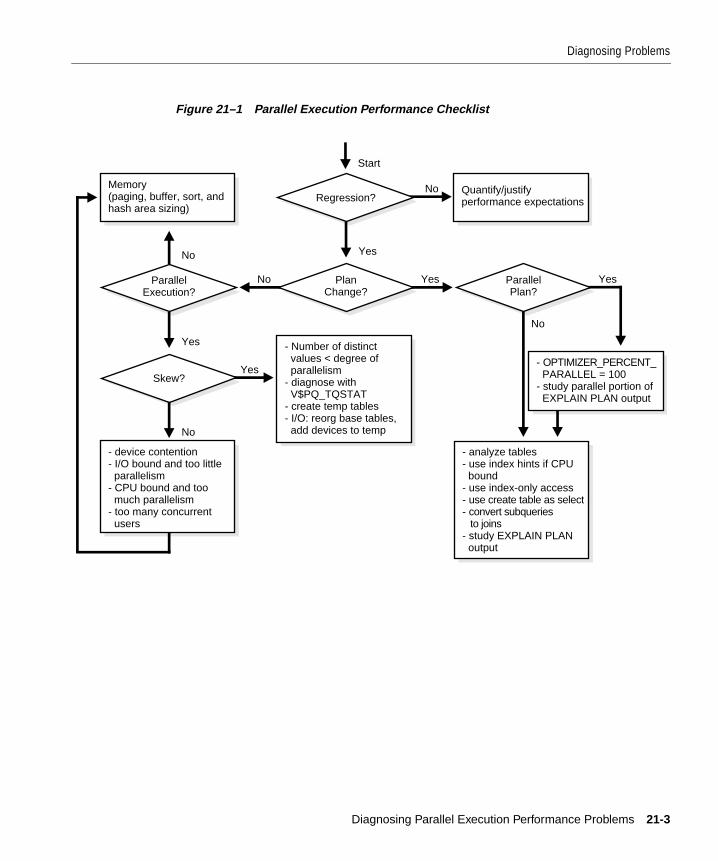
Diagnosing Problems
Figure 21–1 Parallel Execution Performance Checklist
Memory(paging, buffer, sort, and hash area sizing)
Quantify/justifyperformance expectations
ParallelExecution?
- device contention- I/O bound and too little parallelism- CPU bound and too much parallelism- too many concurrent users
Skew?
No
Yes
No
Regression?
PlanChange?
No
Yes
Yes
No
Yes
- Number of distinct values < degree of parallelism- diagnose with V$PQ_TQSTAT- create temp tables- I/O: reorg base tables, add devices to temp
ParallelPlan?
Yes
- OPTIMIZER_PERCENT_ PARALLEL = 100 - study parallel portion of EXPLAIN PLAN output
- analyze tables- use index hints if CPU bound- use index-only access- use create table as select- convert subqueries to joins- study EXPLAIN PLAN output
No
Start
Diagnosing Parallel Execution Performance Problems 21-3
Diagnosing Problems
Is There Regression?Does parallel execution’s actual performance deviate from what you expected? Ifperformance is as you expected, can you justify the notion that there is a perfor-mance problem? Perhaps you have a desired outcome in mind, to which you arecomparing the current outcome. Perhaps you have a justifiable performance expec-tation which the system is not achieving. You might have achieved this level of per-formance or particular execution plan in the past, but now, with a similarenvironment and operation, this is not being met.
If performance is not as you expected, can you quantify the deviation? For datawarehousing operations, the execution plan is key. For critical data warehousingoperations, save the EXPLAIN PLAN results. Then, as you analyze the data, reana-lyze, upgrade Oracle, and load in new data over the course of time, you can com-pare any new execution plan with the old plan. You can take this approach eitherproactively or reactively.
Alternatively, you may find that you get a plan that works better if you use hints.You may want to understand why hints were necessary, and figure out how to getthe optimizer to generate the desired plan without the hints. Try increasing the sta-tistical sample size: better statistics may give you a better plan. If you had to use aPARALLEL hint, look to see whether you had OPTIMIZER_PERCENT_PARALLELset to 100%.
Is There a Plan Change?If there has been a change in the execution plan, determine whether the plan is (orshould be) parallel or serial.
Is There a Parallel Plan?If the execution plan is (or should be) parallel:
■ If you want a parallel plan, but the optimizer has not given you one, try increas-ing OPTIMIZER_PERCENT_PARALLEL to 100 and see if this improves perfor-mance.
■ Study the EXPLAIN PLAN output. Did you analyze all the tables? Perhaps youneed to use hints in a few cases. Verify that the hint gives better results.
See Also: Parallel EXPLAIN PLAN tags are defined in Table 23–2.
21-4 Oracle8 Tuning
Diagnosing Problems
Is There a Serial Plan?If the execution plan is (or should be) serial, consider the following strategies:
■ Use an index. Sometimes adding the right index can greatly improve perfor-mance. Consider adding an extra column to the index: perhaps your operationcould obtain all its data from the index, and not require a table scan. Perhapsyou need to use hints in a few cases. Verify that the hint gives better results.
■ If you do not analyze often, and you can spare the time, it is a good practice tocompute statistics. This particularly important if you are performing manyjoins; it will result in better plans. Alternatively, you can estimate statistics.
Note: Using different sample sizes can cause the plan to change. Generally, thehigher the sample size, the better the plan.
■ Use histograms for non-uniform distributions.
■ Check initialization parameters to be sure the values are reasonable.
■ Replace bind variables with literals.
■ Note whether execution is I/O or CPU bound, then check the optimizer costmodel.
■ Convert subqueries to joins.
■ Use CREATE TABLE ... AS SELECT to break a complex operation into smallerpieces. With a large query referencing five or six tables, it may be difficult todetermine which part of the query is taking the most time. You can isolate thetroublesome parts of the query by breaking it into steps and analyzing eachstep.
See Also: Oracle8 Concepts regarding CREATE TABLE ... AS SELECT"Step 3: Analyzing Data" on page 19-45 regarding COMPUTE and ESTIMATE
Is There Parallel Execution?If the cause of regression cannot be traced to problems in the plan, then the prob-lem must be an execution issue. For data warehousing operations, both serial andparallel, consider memory. Check the paging rate and make sure the system isusing memory as effectively as possible. Check buffer, sort, and hash area sizing.After you run a query or DML operation, you can look at the V$SESSTAT,V$PQ_SESSTAT and V$PQ_SYSSTAT views to see the number of server processesused, and other information for the session and system.
See Also: "Querying the Dynamic Performance Views: Example" on page 21-12
Diagnosing Parallel Execution Performance Problems 21-5
Diagnosing Problems
Is There Skew?If parallel execution is occurring, is there unevenness in workload distribution(skew)? For example, if there are 10 CPUs and a single user, you can see whetherthe workload is evenly distributed across CPUs. This may vary over time, with peri-ods that are more or less I/O intensive, but in general each CPU should haveroughly the same amount of activity.
The statistics in V$PQ_TQSTAT show rows produced and consumed per parallelserver process. This is a good indication of skew, and does not require single useroperation.
Operating system statistics show you the per-processor CPU utilization and per-disk I/O activity. Concurrently running tasks make it harder to see what is goingon, however. It can be useful to run in single-user mode and check operating sys-tem monitors which show system level CPU and I/O activity.
When workload distribution is unbalanced, a common culprit is the presence ofskew in the data. For a hash join, this may be the case if the number of distinct val-ues is less than the degree of parallelism. When joining two tables on a columnwith only 4 distinct values, you will not get scaling on more than 4. If you have 10CPUs, 4 of them will be saturated but 6 will be idle. To avoid this problem, changethe query: use temporary tables to change the join order such that all operationshave more values in the join column than the number of CPUs.
If I/O problems occur you may need to reorganize your data, spreading it overmore devices. If parallel execution problems occur, check to be sure you have fol-lowed the recommendation to spread data over at least as many devices as CPUs.
If there is no skew in workload distribution, check for the following conditions:
■ Is there device contention? Are there enough disk controllers to provide ade-quate I/O bandwidth?
■ Is the system I/O bound, with too little parallelism? If so, consider increasingparallelism up to the number of devices.
■ Is the system CPU bound, with too much parallelism? Check the operating sys-tem CPU monitor to see whether a lot of time is being spent in system calls.The resource may be overcommitted, and too much parallelism may cause pro-cesses to compete with themselves.
■ Are there more concurrent users than the system can support?
21-6 Oracle8 Tuning
Executing Parallel SQL Statements
Executing Parallel SQL StatementsAfter analyzing your tables and indexes, you should be able to run operations andsee speedup that scales linearly with the degree of parallelism used. The followingoperations should scale:
■ table scans
■ nested loop join
■ sort merge join
■ hash join
■ “not in”
■ group by
■ select distinct
■ union and union all
■ aggregation
■ PL/SQL functions called from SQL
■ order by
■ create table as select
■ create index
■ rebuild index
■ rebuild index partition
■ move partition
■ split partition
■ update
■ delete
■ insert ... select
■ enable constraint
■ star transformation
Start with simple parallel operations. Evaluate total I/O throughput with SELECTCOUNT(*) FROM facts. Evaluate total CPU power by adding a complex WHEREclause. I/O imbalance may suggest a better physical database layout. After you
Diagnosing Parallel Execution Performance Problems 21-7
Using EXPLAIN PLAN to See How an Operation Is Parallelized
understand how simple scans work, add aggregation, joins, and other operationsthat reflect individual aspects of the overall workload. Look for bottlenecks.
Besides query performance you should also monitor parallel load, parallel indexcreation, and parallel DML, and look for good utilization of I/O and CPU resources.
Using EXPLAIN PLAN to See How an Operation Is ParallelizedUse an EXPLAIN PLAN statement to view the sequential and parallel operationplan. The OTHER_TAG column of the plan table summarizes how each plan step isparallelized, and describes the text of the operation used by parallel server pro-cesses for each operation. Optimizer cost information for selected plan steps isgiven in the COST, BYTES, and CARDINALITY columns. Table 23–2 summarizesthe meaning of the OTHER_TAG column.
EXPLAIN PLAN thus provides detailed information as to how specific operationsare being performed. You can then change the execution plan for better perfor-mance. For example, if many steps are serial (where OTHER_TAG is blank, serial toparallel, or parallel to serial), then the parallel controller could be a bottleneck. Con-sider the following SQL statement, which summarizes sales data by region:
EXPLAIN PLAN SET STATEMENT_ID = ‘Jan_Summary’ FORSELECT dim_1 SUM(meas1) FROM facts WHERE dim_2 < ‘02-01-1995’GROUP BY dim_1
This script extracts a compact hierarchical plan from the EXPLAIN PLAN output:
SELECTSUBSTR( LPAD(' ',2*(level-1)) ||DECODE(id, 0, statement_id, operation) ||' ' || options || ' ' || object_name ||' [' || partition_start || ',' || partition_stop ||'] ' || other_tag,1, 79) "step [start,stop] par"FROM plan_tableSTART WITH id = 0CONNECT BY PRIOR id = parent_idAND PRIOR NVL(statement_id,' ') =NVL(statement_id);
Following is the query plan for “Jan_Summary”:
Jan_Summary [,]SORT GROUP BY [,] PARALLEL_TO_SERIALTABLE ACCESS FULL facts [NUMBER(1),NUMBER(1)] PARALLEL_TO_PARALLEL;
21-8 Oracle8 Tuning
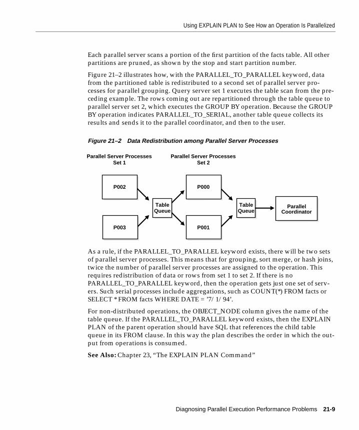
Using EXPLAIN PLAN to See How an Operation Is Parallelized
Each parallel server scans a portion of the first partition of the facts table. All otherpartitions are pruned, as shown by the stop and start partition number.
Figure 21–2 illustrates how, with the PARALLEL_TO_PARALLEL keyword, datafrom the partitioned table is redistributed to a second set of parallel server pro-cesses for parallel grouping. Query server set 1 executes the table scan from the pre-ceding example. The rows coming out are repartitioned through the table queue toparallel server set 2, which executes the GROUP BY operation. Because the GROUPBY operation indicates PARALLEL_TO_SERIAL, another table queue collects itsresults and sends it to the parallel coordinator, and then to the user.
Figure 21–2 Data Redistribution among Parallel Server Processes
As a rule, if the PARALLEL_TO_PARALLEL keyword exists, there will be two setsof parallel server processes. This means that for grouping, sort merge, or hash joins,twice the number of parallel server processes are assigned to the operation. Thisrequires redistribution of data or rows from set 1 to set 2. If there is noPARALLEL_TO_PARALLEL keyword, then the operation gets just one set of serv-ers. Such serial processes include aggregations, such as COUNT(*) FROM facts orSELECT * FROM facts WHERE DATE = ’7/1/94’.
For non-distributed operations, the OBJECT_NODE column gives the name of thetable queue. If the PARALLEL_TO_PARALLEL keyword exists, then the EXPLAINPLAN of the parent operation should have SQL that references the child tablequeue in its FROM clause. In this way the plan describes the order in which the out-put from operations is consumed.
See Also: Chapter 23, “The EXPLAIN PLAN Command”
ParallelCoordinator
Parallel Server ProcessesSet 2
Parallel Server ProcessesSet 1
TableQueue
TableQueue
P001
P002
P003
P000
Diagnosing Parallel Execution Performance Problems 21-9
Using the Dynamic Performance Views
Using the Dynamic Performance ViewsDynamic performance views list internal Oracle8 data structures and statistics thatyou can query periodically to monitor progress of a long-running operation. Whenused in conjunction with data dictionary views, these tables provide a wealth ofinformation. The challenge is visualizing the data and then acting upon it.
Note: On Oracle Parallel Server, global versions of these views aggregate the infor-mation over multiple instances. The global views have analogous names such asGV$FILESTAT for V$FILESTAT, and so on.
See Also: Oracle8 Parallel Server Concepts & Administration for more informationabout global dynamic performance views.
V$FILESTATThis view sums read and write requests, number of blocks, and service times forevery datafile in every tablespace. It can help you diagnose I/O problems andworkload distribution problems.
The file numbers listed in V$FILESTAT can be joined to those in theDBA_DATA_FILES view to group I/O by tablespace or to find the filename for agiven file number. By doing ratio analysis you can determine the percentage of thetotal tablespace activity used by each file in the tablespace. If you make a practiceof putting just one large, heavily accessed object in a tablespace, you can use thistechnique to identify objects that have a poor physical layout.
You can further diagnose disk space allocation problems using the DBA_EXTENTSview. Ensure that space is allocated evenly from all files in the tablespace. Monitor-ing V$FILESTAT during a long-running operation and correlating I/O activity tothe EXPLAIN PLAN output is a good way to follow progress.
V$PARAMETERThis view lists the name, current value, and default value of all system parameters.In addition, the view indicates whether the parameter may be modified online withan ALTER SYSTEM or ALTER SESSION command.
V$PQ_SESSTATThis view is valid only when queried from a session that is executing parallel SQLstatements. Thus it cannot be used to monitor a long running operation. It givessummary statistics about the parallel statements executed in the session, includingtotal number of messages exchanged between server processes and the actual num-ber of parallel server processes used.
21-10 Oracle8 Tuning
Using the Dynamic Performance Views
V$PQ_SLAVEThis view tallies the current and total CPU time and number of messages sent andreceived per parallel server process. It can be monitored during a long-runningoperation. Verify that there is little variance among processes in CPU usage andnumber of messages processed. A variance may indicate a load-balancing problem.Attempt to correlate the variance to a variance in the base data distribution.Extreme imbalance could indicate that the number of distinct values in a join col-umn is much less than the degree of parallelism. See “Parallel CREATE TABLE ...AS SELECT” in Oracle8 Concepts for a possible workaround.
V$PQ_SYSSTATThe V$PQ_SYSSTAT view aggregates session statistics from all parallel server pro-cesses. It sums the total parallel server message traffic, and gives the status of thepool of parallel server processes.
This view can help you determine the appropriate number of parallel server pro-cesses for an instance. The statistics that are particularly useful are “Servers Busy”,“Servers Idle”, “Servers Started”, and “Servers Shutdown”.
Periodically examine V$PQ_SYSSTAT to determine whether the parallel server pro-cesses for the instance are actually busy, as follows:
SELECT * FROM V$PQ_SYSSTATWHERE statistic = ”Servers Busy”;
STATISTIC VALUE--------------------- -----------Servers Busy 70
V$PQ_TQSTATThis view provides a detailed report of message traffic at the level of the tablequeue. It is valid only when queried from a session that is executing parallel SQLstatements. A table queue is the pipeline between parallel server groups orbetween the parallel coordinator and a parallel server group or between a parallelserver group and the coordinator. These table queues are represented in the plan bythe tags PARALLEL_TO_PARALLEL, SERIAL_TO_PARALLEL, orPARALLEL_TO_SERIAL, respectively.
The view contains a row for each parallel server process that reads or writes eachtable queue. A table queue connecting 10 consumers to 10 producers will have 20rows in the view. Sum the bytes column and group by TQ_ID (table queue identi-fier) for the total number of bytes sent through each table queue. Compare this with
Diagnosing Parallel Execution Performance Problems 21-11
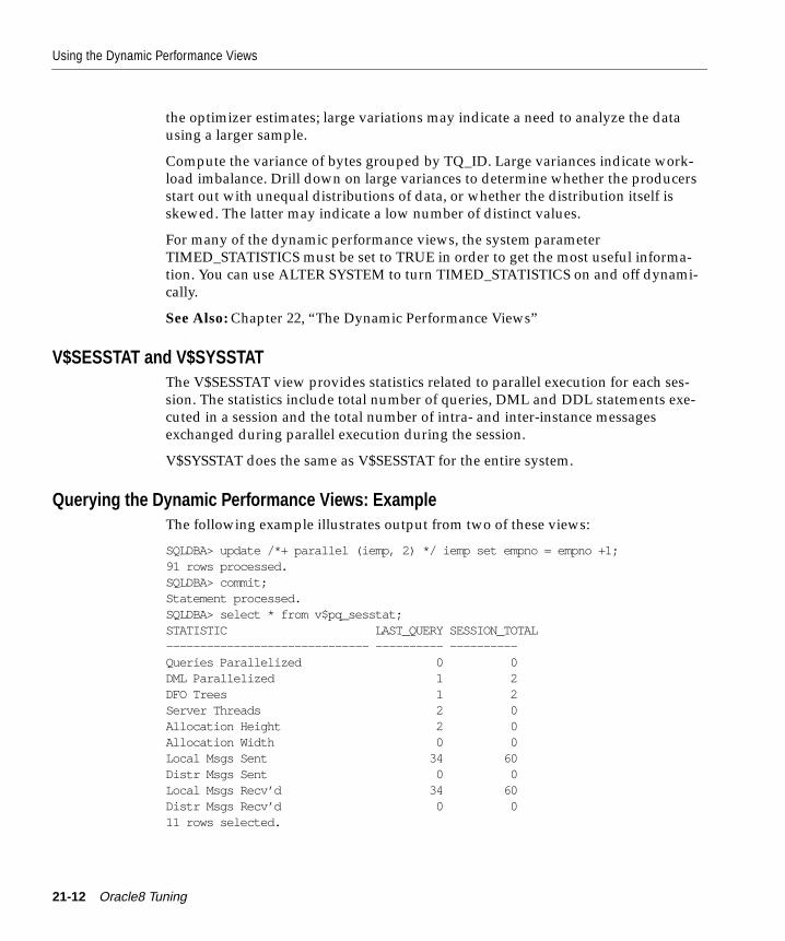
Using the Dynamic Performance Views
the optimizer estimates; large variations may indicate a need to analyze the datausing a larger sample.
Compute the variance of bytes grouped by TQ_ID. Large variances indicate work-load imbalance. Drill down on large variances to determine whether the producersstart out with unequal distributions of data, or whether the distribution itself isskewed. The latter may indicate a low number of distinct values.
For many of the dynamic performance views, the system parameterTIMED_STATISTICS must be set to TRUE in order to get the most useful informa-tion. You can use ALTER SYSTEM to turn TIMED_STATISTICS on and off dynami-cally.
See Also: Chapter 22, “The Dynamic Performance Views”
V$SESSTAT and V$SYSSTATThe V$SESSTAT view provides statistics related to parallel execution for each ses-sion. The statistics include total number of queries, DML and DDL statements exe-cuted in a session and the total number of intra- and inter-instance messagesexchanged during parallel execution during the session.
V$SYSSTAT does the same as V$SESSTAT for the entire system.
Querying the Dynamic Performance Views: ExampleThe following example illustrates output from two of these views:
SQLDBA> update /*+ parallel (iemp, 2) */ iemp set empno = empno +1;91 rows processed.SQLDBA> commit;Statement processed.SQLDBA> select * from v$pq_sesstat;STATISTIC LAST_QUERY SESSION_TOTAL------------------------------ ---------- ----------Queries Parallelized 0 0DML Parallelized 1 2DFO Trees 1 2Server Threads 2 0Allocation Height 2 0Allocation Width 0 0Local Msgs Sent 34 60Distr Msgs Sent 0 0Local Msgs Recv’d 34 60Distr Msgs Recv’d 0 011 rows selected.
21-12 Oracle8 Tuning

Using the Dynamic Performance Views
SQLDBA> select * from v$pq_sysstat;STATISTIC VALUE------------------------------ ----------Servers Busy 0Servers Idle 2Servers Highwater 2Server Sessions 4Servers Started 2Servers Shutdown 0Servers Cleaned Up 0Queries Initiated 0DML Initiated 2DFO Trees 2Local Msgs Sent 60Distr Msgs Sent 0Local Msgs Recv’d 60Distr Msgs Recv’d 015 rows selected.
In V$PQ_SESSTAT, some of the statistics provide the following information.
In V$PQ_SYSSTAT, the “DML Initiated” statistic indicates the number of DMLoperations done in the system.
Note that statements such as INSERT ... SELECT are treated as a single DML state-ment, not as one DML statement and one query.
See Also: Oracle8 SQL Reference for information about statistics.
DML Parallelized number of statements with insert, delete andupdate that were parallelized by the last operationand by this session
Queries Parallelized number of all other parallel statements
DFO Trees number of fragments of query plan that were par-allelized
Server Threads total number of server processes (typically 2xdegree)
Allocation Height requested number of servers on each instance
Allocation Width requested number of instances
Diagnosing Parallel Execution Performance Problems 21-13
Checking Operating System Statistics
Checking Operating System StatisticsThere is considerable overlap between information available in Oracle and informa-tion available though operating system utilities (such as sar and vmstat on UNIX-based systems). Operating systems provide performance statistics on I/O, commu-nication, CPU, memory and paging, scheduling, and synchronization primitives.The Oracle V$SESSTAT view provides the major categories of OS statistics as well.
Typically, Operating system information about I/O devices and semaphore opera-tions is harder to map back to database objects and operations than is Oracle infor-mation. However, some operating systems have good visualization tools andefficient means of collecting the data.
Operating system information about CPU and memory usage is very important forassessing performance. Probably the most important statistic is CPU usage. Thegoal of low -level performance tuning is to become CPU bound on all CPUs. Oncethis is achieved, you can move up a level and work at the SQL level to find an alter-nate plan that might be more I/O intensive but uses less CPU.
Operating system memory and paging information is valuable for fine tuning themany system parameters that control how memory is divided among memory-intensive warehouse subsystems like parallel communication, sort, and hash join.
Minimum Recovery TimeIf the system requires ten minutes to run an operation, it will take at least 10 min-utes to roll back the operation: this is the best performance achievable. If there issome instance failure and some system failure, then recovery time will increasebecause not all the server processes are available to provide rollback.
21-14 Oracle8 Tuning
Parallel DML Restrictions
Parallel DML RestrictionsYou must either commit or roll back directly after you issue a parallel INSERT,UPDATE, or DELETE statement, or a serial insert with the APPEND hint. You canperform no other SQL commands until this is done.
Discrete transactions are not supported for parallel DML.
A session that is enabled for parallel DML may put transactions in the session in aspecial mode. If any DML statement in a transaction modifies a table in parallel, nosubsequent serial or parallel query or DML statement can access the same tableagain in that transaction. This means that the results of parallel modifications can-not be seen during the transaction.
A complete listing of parallel DML and direct-load insert restrictions is found inOracle8 Concepts. If a parallel restriction is violated, the operation is simply per-formed serially. If a direct-load insert restriction is violated, then the APPEND hintis ignored and a conventional insert is performed. No error message is returned.
Diagnosing Parallel Execution Performance Problems 21-15

Parallel DML Restrictions
21-16 Oracle8 Tuning

Part VI
Performance Diagnostic ToolsPart VI discusses the tools available to diagnose system problems and tune systemperformance. The chapters in Part VI are:
■ Chapter 22, “The Dynamic Performance Views”
■ Chapter 23, “The EXPLAIN PLAN Command”
■ Chapter 24, “The SQL Trace Facility and TKPROF”
■ Chapter 25, “Using Oracle Trace”
■ Chapter 26, “Registering Applications”

The Dynamic Performance
22
The Dynamic Performance ViewsDynamic performance views are useful for identifying instance-level performanceproblems. Whereas the underlying X$ tables represent internal data structures thatcan be modified by SQL statements, the V$ views allow users other than SYS read-only access to this data. This chapter describes the views of the greatest use forboth performance tuning and ad hoc investigation—for example, when usersreport a sudden deterioration in response time.
■ Instance-Level Views for Tuning
■ Session-Level or Transient Views for Tuning
■ Current Statistic Value and Rate of Change
See Also: For complete information on all dynamic performance tables, see Oracle8Reference.
Views 22-1
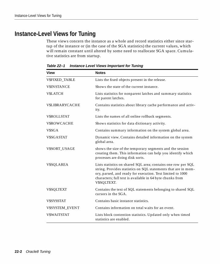
Instance-Level Views for Tuning
Instance-Level Views for TuningThese views concern the instance as a whole and record statistics either since star-tup of the instance or (in the case of the SGA statistics) the current values, whichwill remain constant until altered by some need to reallocate SGA space. Cumula-tive statistics are from startup.
Table 22–1 Instance Level Views Important for Tuning
View Notes
V$FIXED_TABLE Lists the fixed objects present in the release.
V$INSTANCE Shows the state of the current instance.
V$LATCH Lists statistics for nonparent latches and summary statisticsfor parent latches.
V$LIBRARYCACHE Contains statistics about library cache performance and activ-ity.
V$ROLLSTAT Lists the names of all online rollback segments.
V$ROWCACHE Shows statistics for data dictionary activity.
V$SGA Contains summary information on the system global area.
V$SGASTAT Dynamic view. Contains detailed information on the systemglobal area.
V$SORT_USAGE shows the size of the temporary segments and the sessioncreating them. This information can help you identify whichprocesses are doing disk sorts.
V$SQLAREA Lists statistics on shared SQL area; contains one row per SQLstring. Provides statistics on SQL statements that are in mem-ory, parsed, and ready for execution. Text limited to 1000characters; full text is available in 64 byte chunks fromV$SQLTEXT.
V$SQLTEXT Contains the text of SQL statements belonging to shared SQLcursors in the SGA.
V$SYSSTAT Contains basic instance statistics.
V$SYSTEM_EVENT Contains information on total waits for an event.
V$WAITSTAT Lists block contention statistics. Updated only when timedstatistics are enabled.
22-2 Oracle8 Tuning
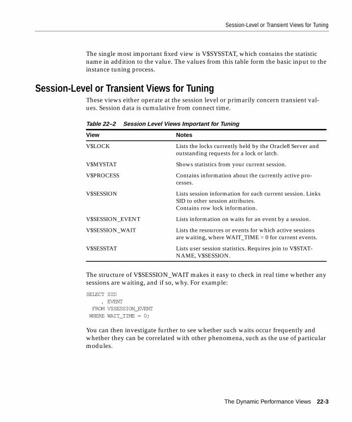
Session-Level or Transient Views for Tuning
The single most important fixed view is V$SYSSTAT, which contains the statisticname in addition to the value. The values from this table form the basic input to theinstance tuning process.
Session-Level or Transient Views for TuningThese views either operate at the session level or primarily concern transient val-ues. Session data is cumulative from connect time.
The structure of V$SESSION_WAIT makes it easy to check in real time whether anysessions are waiting, and if so, why. For example:
SELECT SID , EVENT FROM V$SESSION_EVENT WHERE WAIT_TIME = 0;
You can then investigate further to see whether such waits occur frequently andwhether they can be correlated with other phenomena, such as the use of particularmodules.
Table 22–2 Session Level Views Important for Tuning
View Notes
V$LOCK Lists the locks currently held by the Oracle8 Server andoutstanding requests for a lock or latch.
V$MYSTAT Shows statistics from your current session.
V$PROCESS Contains information about the currently active pro-cesses.
V$SESSION Lists session information for each current session. LinksSID to other session attributes.Contains row lock information.
V$SESSION_EVENT Lists information on waits for an event by a session.
V$SESSION_WAIT Lists the resources or events for which active sessionsare waiting, where WAIT_TIME = 0 for current events.
V$SESSTAT Lists user session statistics. Requires join to V$STAT-NAME, V$SESSION.
The Dynamic Performance Views 22-3
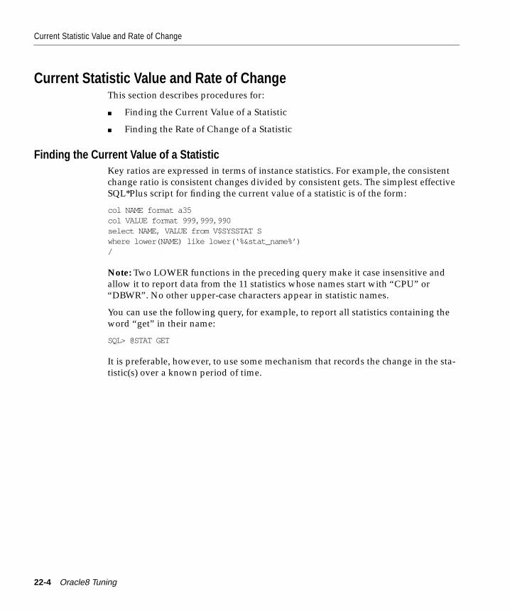
Current Statistic Value and Rate of Change
Current Statistic Value and Rate of ChangeThis section describes procedures for:
■ Finding the Current Value of a Statistic
■ Finding the Rate of Change of a Statistic
Finding the Current Value of a StatisticKey ratios are expressed in terms of instance statistics. For example, the consistentchange ratio is consistent changes divided by consistent gets. The simplest effectiveSQL*Plus script for finding the current value of a statistic is of the form:
col NAME format a35col VALUE format 999,999,990select NAME, VALUE from V$SYSSTAT Swhere lower(NAME) like lower(‘%&stat_name%’)/
Note: Two LOWER functions in the preceding query make it case insensitive andallow it to report data from the 11 statistics whose names start with “CPU” or“DBWR”. No other upper-case characters appear in statistic names.
You can use the following query, for example, to report all statistics containing theword “get” in their name:
SQL> @STAT GET
It is preferable, however, to use some mechanism that records the change in the sta-tistic(s) over a known period of time.
22-4 Oracle8 Tuning
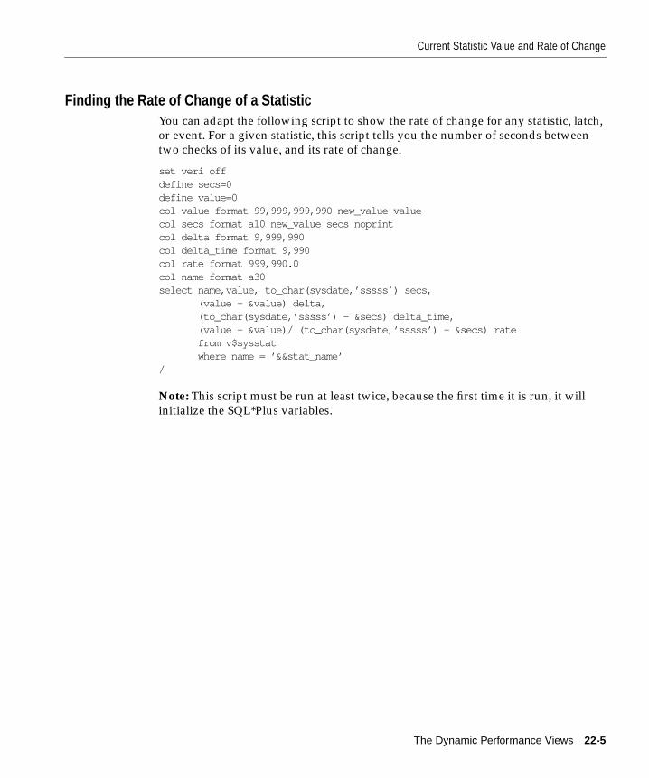
Current Statistic Value and Rate of Change
Finding the Rate of Change of a StatisticYou can adapt the following script to show the rate of change for any statistic, latch,or event. For a given statistic, this script tells you the number of seconds betweentwo checks of its value, and its rate of change.
set veri offdefine secs=0define value=0col value format 99,999,999,990 new_value valuecol secs format a10 new_value secs noprintcol delta format 9,999,990col delta_time format 9,990col rate format 999,990.0col name format a30select name,value, to_char(sysdate,’sssss’) secs, (value - &value) delta, (to_char(sysdate,’sssss’) - &secs) delta_time, (value - &value)/ (to_char(sysdate,’sssss’) - &secs) rate from v$sysstat where name = ’&&stat_name’/
Note: This script must be run at least twice, because the first time it is run, it willinitialize the SQL*Plus variables.
The Dynamic Performance Views 22-5

Current Statistic Value and Rate of Change
22-6 Oracle8 Tuning
The EXPLAIN PLAN Com
23
The EXPLAIN PLAN CommandThis chapter shows how to use the SQL command EXPLAIN PLAN. It covers thefollowing topics:
■ Introduction
■ Creating the Output Table
■ Output Table Columns
■ Formatting EXPLAIN PLAN Output
■ EXPLAIN PLAN Restrictions
See Also: For the syntax of the EXPLAIN PLAN command, see the Oracle8 SQL Ref-erence.
mand 23-1
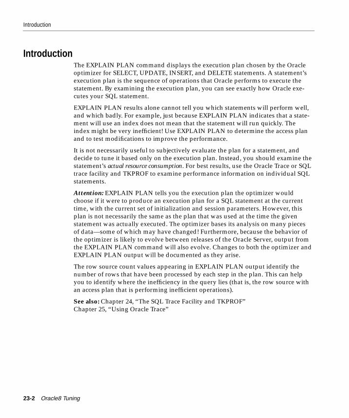
Introduction
IntroductionThe EXPLAIN PLAN command displays the execution plan chosen by the Oracleoptimizer for SELECT, UPDATE, INSERT, and DELETE statements. A statement’sexecution plan is the sequence of operations that Oracle performs to execute thestatement. By examining the execution plan, you can see exactly how Oracle exe-cutes your SQL statement.
EXPLAIN PLAN results alone cannot tell you which statements will perform well,and which badly. For example, just because EXPLAIN PLAN indicates that a state-ment will use an index does not mean that the statement will run quickly. Theindex might be very inefficient! Use EXPLAIN PLAN to determine the access planand to test modifications to improve the performance.
It is not necessarily useful to subjectively evaluate the plan for a statement, anddecide to tune it based only on the execution plan. Instead, you should examine thestatement’s actual resource consumption. For best results, use the Oracle Trace or SQLtrace facility and TKPROF to examine performance information on individual SQLstatements.
Attention: EXPLAIN PLAN tells you the execution plan the optimizer wouldchoose if it were to produce an execution plan for a SQL statement at the currenttime, with the current set of initialization and session parameters. However, thisplan is not necessarily the same as the plan that was used at the time the givenstatement was actually executed. The optimizer bases its analysis on many piecesof data—some of which may have changed! Furthermore, because the behavior ofthe optimizer is likely to evolve between releases of the Oracle Server, output fromthe EXPLAIN PLAN command will also evolve. Changes to both the optimizer andEXPLAIN PLAN output will be documented as they arise.
The row source count values appearing in EXPLAIN PLAN output identify thenumber of rows that have been processed by each step in the plan. This can helpyou to identify where the inefficiency in the query lies (that is, the row source withan access plan that is performing inefficient operations).
See also: Chapter 24, “The SQL Trace Facility and TKPROF”Chapter 25, “Using Oracle Trace”
23-2 Oracle8 Tuning
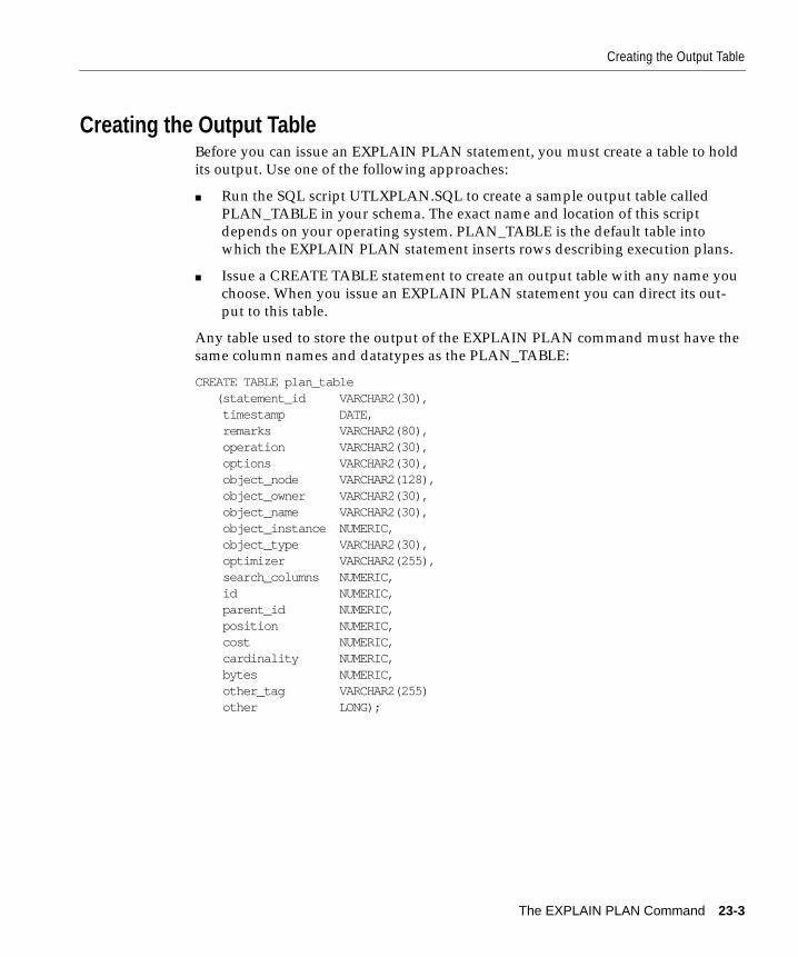
Creating the Output Table
Creating the Output TableBefore you can issue an EXPLAIN PLAN statement, you must create a table to holdits output. Use one of the following approaches:
■ Run the SQL script UTLXPLAN.SQL to create a sample output table calledPLAN_TABLE in your schema. The exact name and location of this scriptdepends on your operating system. PLAN_TABLE is the default table intowhich the EXPLAIN PLAN statement inserts rows describing execution plans.
■ Issue a CREATE TABLE statement to create an output table with any name youchoose. When you issue an EXPLAIN PLAN statement you can direct its out-put to this table.
Any table used to store the output of the EXPLAIN PLAN command must have thesame column names and datatypes as the PLAN_TABLE:
CREATE TABLE plan_table (statement_id VARCHAR2(30), timestamp DATE, remarks VARCHAR2(80), operation VARCHAR2(30), options VARCHAR2(30), object_node VARCHAR2(128), object_owner VARCHAR2(30), object_name VARCHAR2(30), object_instance NUMERIC, object_type VARCHAR2(30), optimizer VARCHAR2(255), search_columns NUMERIC, id NUMERIC, parent_id NUMERIC, position NUMERIC, cost NUMERIC, cardinality NUMERIC, bytes NUMERIC, other_tag VARCHAR2(255) other LONG);
The EXPLAIN PLAN Command 23-3

Output Table Columns
Output Table ColumnsThe PLAN_TABLE used by the EXPLAIN PLAN command contains the followingcolumns:
Table 23–1 PLAN_TABLE Columns
Column Description
STATEMENT_ID The value of the optional STATEMENT_ID parameter speci-fied in the EXPLAIN PLAN statement.
TIMESTAMP The date and time when the EXPLAIN PLAN statement wasissued.
REMARKS Any comment (of up to 80 bytes) you wish to associate witheach step of the explained plan. If you need to add or changea remark on any row of the PLAN_TABLE, use the UPDATEstatement to modify the rows of the PLAN_TABLE.
OPERATION The name of the internal operation performed in this step. Inthe first row generated for a statement, the column containsone of the following values:
DELETE STATEMENT
INSERT STATEMENT
SELECT STATEMENT
UPDATE STATEMENT
OPTIONS A variation on the operation described in the OPERATIONcolumn.
OBJECT_NODE The name of the database link used to reference the object (atable name or view name). For local queries using the parallelquery option, this column describes the order in which outputfrom operations is consumed.
OBJECT_OWNER The name of the user who owns the schema containing thetable or index.
OBJECT_NAME The name of the table or index.
OBJECT_INSTANCE A number corresponding to the ordinal position of the objectas it appears in the original statement. The numbering pro-ceeds from left to right, outer to inner with respect to the origi-nal statement text. Note that view expansion will result inunpredictable numbers.
23-4 Oracle8 Tuning
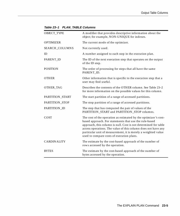
Output Table Columns
OBJECT_TYPE A modifier that provides descriptive information about theobject; for example, NON-UNIQUE for indexes.
OPTIMIZER The current mode of the optimizer.
SEARCH_COLUMNS Not currently used.
ID A number assigned to each step in the execution plan.
PARENT_ID The ID of the next execution step that operates on the outputof the ID step.
POSITION The order of processing for steps that all have the samePARENT_ID.
OTHER Other information that is specific to the execution step that auser may find useful.
OTHER_TAG Describes the contents of the OTHER column. See Table 23–2for more information on the possible values for this column.
PARTITION_START The start partition of a range of accessed partitions.
PARTITION_STOP The stop partition of a range of accessed partitions.
PARTITION_ID The step that has computed the pair of values of thePARTITION_START and PARTITION_STOP columns.
COST The cost of the operation as estimated by the optimizer’s cost-based approach. For statements that use the rule-basedapproach, this column is null. Cost is not determined for tableaccess operations. The value of this column does not have anyparticular unit of measurement, it is merely a weighted valueused to compare costs of execution plans.
CARDINALITY The estimate by the cost-based approach of the number ofrows accessed by the operation.
BYTES The estimate by the cost-based approach of the number ofbytes accessed by the operation.
Table 23–1 PLAN_TABLE Columns
The EXPLAIN PLAN Command 23-5
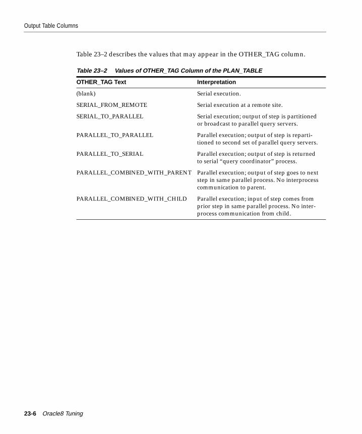
Output Table Columns
Table 23–2 describes the values that may appear in the OTHER_TAG column.
Table 23–2 Values of OTHER_TAG Column of the PLAN_TABLE
OTHER_TAG Text Interpretation
(blank) Serial execution.
SERIAL_FROM_REMOTE Serial execution at a remote site.
SERIAL_TO_PARALLEL Serial execution; output of step is partitionedor broadcast to parallel query servers.
PARALLEL_TO_PARALLEL Parallel execution; output of step is reparti-tioned to second set of parallel query servers.
PARALLEL_TO_SERIAL Parallel execution; output of step is returnedto serial “query coordinator” process.
PARALLEL_COMBINED_WITH_PARENT Parallel execution; output of step goes to nextstep in same parallel process. No interprocesscommunication to parent.
PARALLEL_COMBINED_WITH_CHILD Parallel execution; input of step comes fromprior step in same parallel process. No inter-process communication from child.
23-6 Oracle8 Tuning
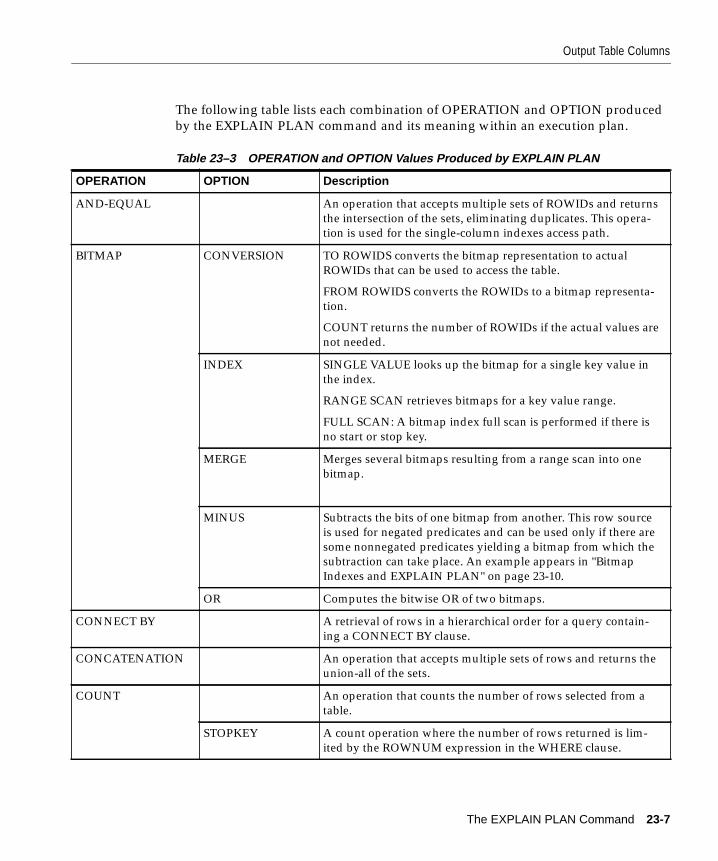
Output Table Columns
The following table lists each combination of OPERATION and OPTION producedby the EXPLAIN PLAN command and its meaning within an execution plan.
Table 23–3 OPERATION and OPTION Values Produced by EXPLAIN PLAN
OPERATION OPTION Description
AND-EQUAL An operation that accepts multiple sets of ROWIDs and returnsthe intersection of the sets, eliminating duplicates. This opera-tion is used for the single-column indexes access path.
BITMAP CONVERSION TO ROWIDS converts the bitmap representation to actualROWIDs that can be used to access the table.
FROM ROWIDS converts the ROWIDs to a bitmap representa-tion.
COUNT returns the number of ROWIDs if the actual values arenot needed.
INDEX SINGLE VALUE looks up the bitmap for a single key value inthe index.
RANGE SCAN retrieves bitmaps for a key value range.
FULL SCAN: A bitmap index full scan is performed if there isno start or stop key.
MERGE Merges several bitmaps resulting from a range scan into onebitmap.
MINUS Subtracts the bits of one bitmap from another. This row sourceis used for negated predicates and can be used only if there aresome nonnegated predicates yielding a bitmap from which thesubtraction can take place. An example appears in "BitmapIndexes and EXPLAIN PLAN" on page 23-10.
OR Computes the bitwise OR of two bitmaps.
CONNECT BY A retrieval of rows in a hierarchical order for a query contain-ing a CONNECT BY clause.
CONCATENATION An operation that accepts multiple sets of rows and returns theunion-all of the sets.
COUNT An operation that counts the number of rows selected from atable.
STOPKEY A count operation where the number of rows returned is lim-ited by the ROWNUM expression in the WHERE clause.
The EXPLAIN PLAN Command 23-7
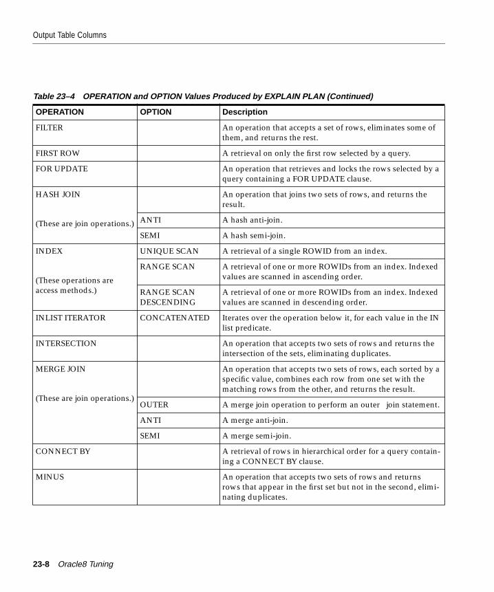
Output Table Columns
Table 23–4 OPERATION and OPTION Values Produced by EXPLAIN PLAN (Continued)
OPERATION OPTION Description
FILTER An operation that accepts a set of rows, eliminates some ofthem, and returns the rest.
FIRST ROW A retrieval on only the first row selected by a query.
FOR UPDATE An operation that retrieves and locks the rows selected by aquery containing a FOR UPDATE clause.
HASH JOIN
(These are join operations.)
An operation that joins two sets of rows, and returns theresult.
ANTI A hash anti-join.
SEMI A hash semi-join.
INDEX
(These operations areaccess methods.)
UNIQUE SCAN A retrieval of a single ROWID from an index.
RANGE SCAN A retrieval of one or more ROWIDs from an index. Indexedvalues are scanned in ascending order.
RANGE SCANDESCENDING
A retrieval of one or more ROWIDs from an index. Indexedvalues are scanned in descending order.
INLIST ITERATOR CONCATENATED Iterates over the operation below it, for each value in the INlist predicate.
INTERSECTION An operation that accepts two sets of rows and returns theintersection of the sets, eliminating duplicates.
MERGE JOIN
(These are join operations.)
An operation that accepts two sets of rows, each sorted by aspecific value, combines each row from one set with thematching rows from the other, and returns the result.
OUTER A merge join operation to perform an outer join statement.
ANTI A merge anti-join.
SEMI A merge semi-join.
CONNECT BY A retrieval of rows in hierarchical order for a query contain-ing a CONNECT BY clause.
MINUS An operation that accepts two sets of rows and returnsrows that appear in the first set but not in the second, elimi-nating duplicates.
23-8 Oracle8 Tuning
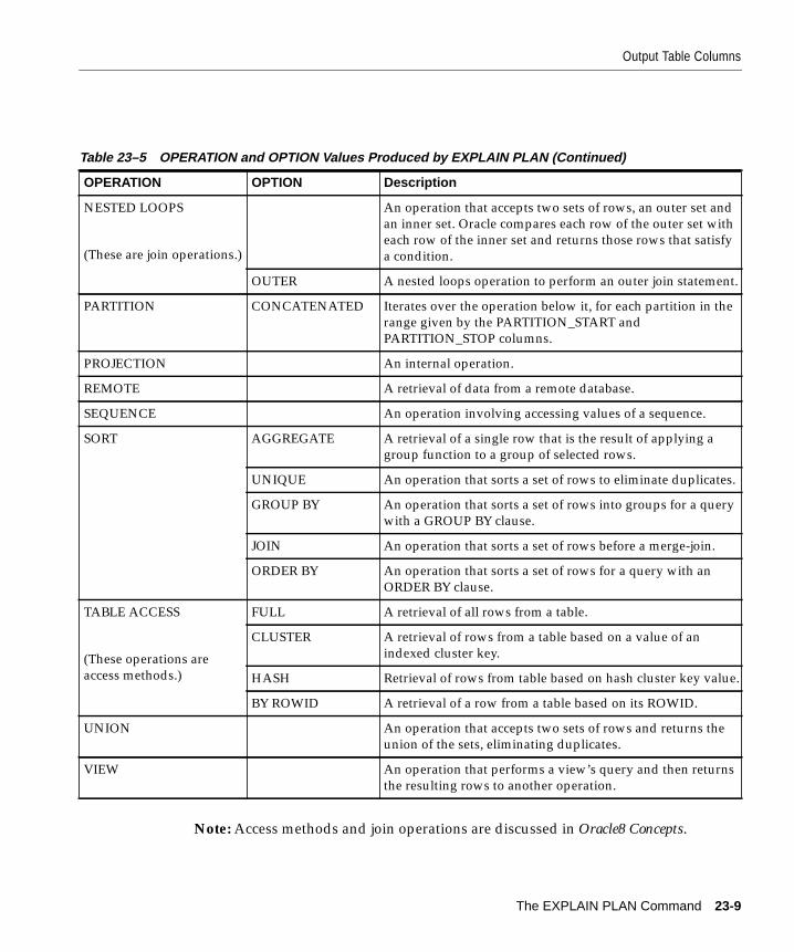
Output Table Columns
Note: Access methods and join operations are discussed in Oracle8 Concepts.
Table 23–5 OPERATION and OPTION Values Produced by EXPLAIN PLAN (Continued)
OPERATION OPTION Description
NESTED LOOPS
(These are join operations.)
An operation that accepts two sets of rows, an outer set andan inner set. Oracle compares each row of the outer set witheach row of the inner set and returns those rows that satisfya condition.
OUTER A nested loops operation to perform an outer join statement.
PARTITION CONCATENATED Iterates over the operation below it, for each partition in therange given by the PARTITION_START andPARTITION_STOP columns.
PROJECTION An internal operation.
REMOTE A retrieval of data from a remote database.
SEQUENCE An operation involving accessing values of a sequence.
SORT AGGREGATE A retrieval of a single row that is the result of applying agroup function to a group of selected rows.
UNIQUE An operation that sorts a set of rows to eliminate duplicates.
GROUP BY An operation that sorts a set of rows into groups for a querywith a GROUP BY clause.
JOIN An operation that sorts a set of rows before a merge-join.
ORDER BY An operation that sorts a set of rows for a query with anORDER BY clause.
TABLE ACCESS
(These operations areaccess methods.)
FULL A retrieval of all rows from a table.
CLUSTER A retrieval of rows from a table based on a value of anindexed cluster key.
HASH Retrieval of rows from table based on hash cluster key value.
BY ROWID A retrieval of a row from a table based on its ROWID.
UNION An operation that accepts two sets of rows and returns theunion of the sets, eliminating duplicates.
VIEW An operation that performs a view’s query and then returnsthe resulting rows to another operation.
The EXPLAIN PLAN Command 23-9
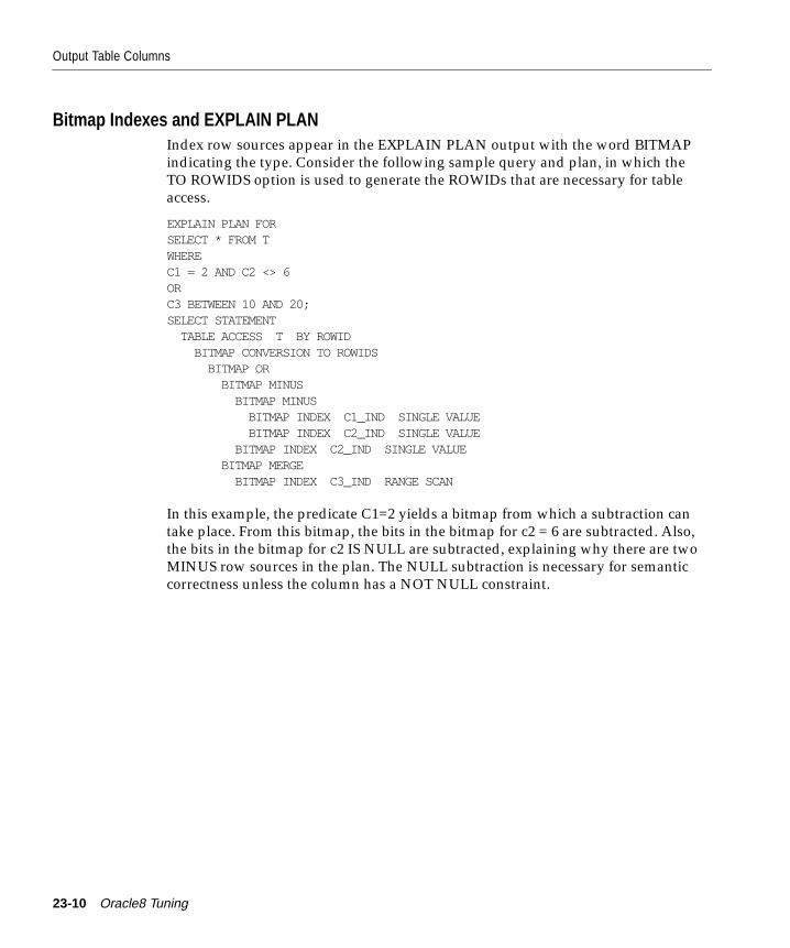
Output Table Columns
Bitmap Indexes and EXPLAIN PLANIndex row sources appear in the EXPLAIN PLAN output with the word BITMAPindicating the type. Consider the following sample query and plan, in which theTO ROWIDS option is used to generate the ROWIDs that are necessary for tableaccess.
EXPLAIN PLAN FORSELECT * FROM TWHEREC1 = 2 AND C2 <> 6ORC3 BETWEEN 10 AND 20;SELECT STATEMENT TABLE ACCESS T BY ROWID BITMAP CONVERSION TO ROWIDS BITMAP OR BITMAP MINUS BITMAP MINUS BITMAP INDEX C1_IND SINGLE VALUE BITMAP INDEX C2_IND SINGLE VALUE BITMAP INDEX C2_IND SINGLE VALUE BITMAP MERGE BITMAP INDEX C3_IND RANGE SCAN
In this example, the predicate C1=2 yields a bitmap from which a subtraction cantake place. From this bitmap, the bits in the bitmap for c2 = 6 are subtracted. Also,the bits in the bitmap for c2 IS NULL are subtracted, explaining why there are twoMINUS row sources in the plan. The NULL subtraction is necessary for semanticcorrectness unless the column has a NOT NULL constraint.
23-10 Oracle8 Tuning
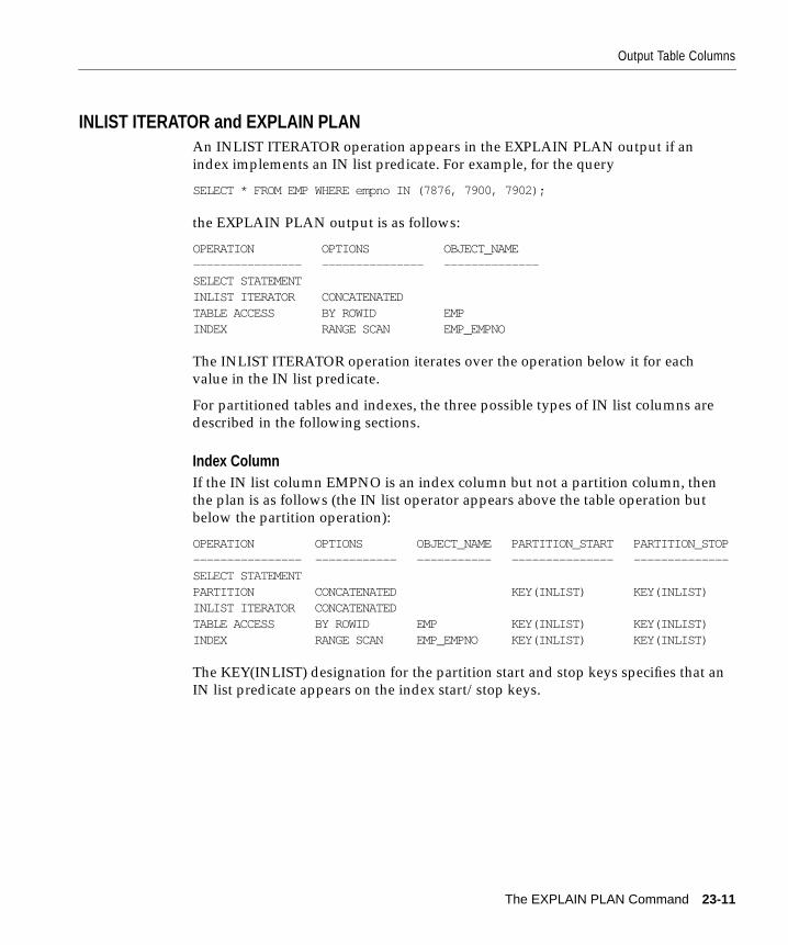
Output Table Columns
INLIST ITERATOR and EXPLAIN PLANAn INLIST ITERATOR operation appears in the EXPLAIN PLAN output if anindex implements an IN list predicate. For example, for the query
SELECT * FROM EMP WHERE empno IN (7876, 7900, 7902);
the EXPLAIN PLAN output is as follows:
OPERATION OPTIONS OBJECT_NAME---------------- --------------- --------------SELECT STATEMENTINLIST ITERATOR CONCATENATEDTABLE ACCESS BY ROWID EMPINDEX RANGE SCAN EMP_EMPNO
The INLIST ITERATOR operation iterates over the operation below it for eachvalue in the IN list predicate.
For partitioned tables and indexes, the three possible types of IN list columns aredescribed in the following sections.
Index ColumnIf the IN list column EMPNO is an index column but not a partition column, thenthe plan is as follows (the IN list operator appears above the table operation butbelow the partition operation):
OPERATION OPTIONS OBJECT_NAME PARTITION_START PARTITION_STOP---------------- ------------ ----------- --------------- --------------SELECT STATEMENTPARTITION CONCATENATED KEY(INLIST) KEY(INLIST)INLIST ITERATOR CONCATENATEDTABLE ACCESS BY ROWID EMP KEY(INLIST) KEY(INLIST)INDEX RANGE SCAN EMP_EMPNO KEY(INLIST) KEY(INLIST)
The KEY(INLIST) designation for the partition start and stop keys specifies that anIN list predicate appears on the index start/stop keys.
The EXPLAIN PLAN Command 23-11
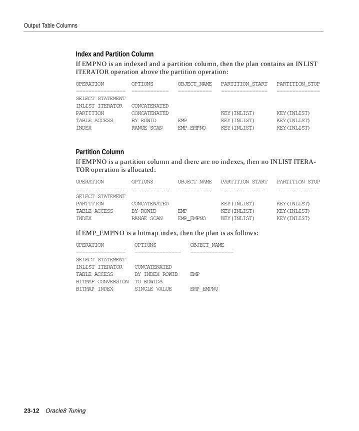
Output Table Columns
Index and Partition ColumnIf EMPNO is an indexed and a partition column, then the plan contains an INLISTITERATOR operation above the partition operation:
OPERATION OPTIONS OBJECT_NAME PARTITION_START PARTITION_STOP---------------- ------------ ----------- --------------- --------------SELECT STATEMENTINLIST ITERATOR CONCATENATEDPARTITION CONCATENATED KEY(INLIST) KEY(INLIST)TABLE ACCESS BY ROWID EMP KEY(INLIST) KEY(INLIST)INDEX RANGE SCAN EMP_EMPNO KEY(INLIST) KEY(INLIST)
Partition ColumnIf EMPNO is a partition column and there are no indexes, then no INLIST ITERA-TOR operation is allocated:
OPERATION OPTIONS OBJECT_NAME PARTITION_START PARTITION_STOP---------------- ------------ ----------- --------------- --------------SELECT STATEMENTPARTITION CONCATENATED KEY(INLIST) KEY(INLIST)TABLE ACCESS BY ROWID EMP KEY(INLIST) KEY(INLIST)INDEX RANGE SCAN EMP_EMPNO KEY(INLIST) KEY(INLIST)
If EMP_EMPNO is a bitmap index, then the plan is as follows:
OPERATION OPTIONS OBJECT_NAME---------------- --------------- --------------SELECT STATEMENTINLIST ITERATOR CONCATENATEDTABLE ACCESS BY INDEX ROWID EMPBITMAP CONVERSION TO ROWIDSBITMAP INDEX SINGLE VALUE EMP_EMPNO
23-12 Oracle8 Tuning
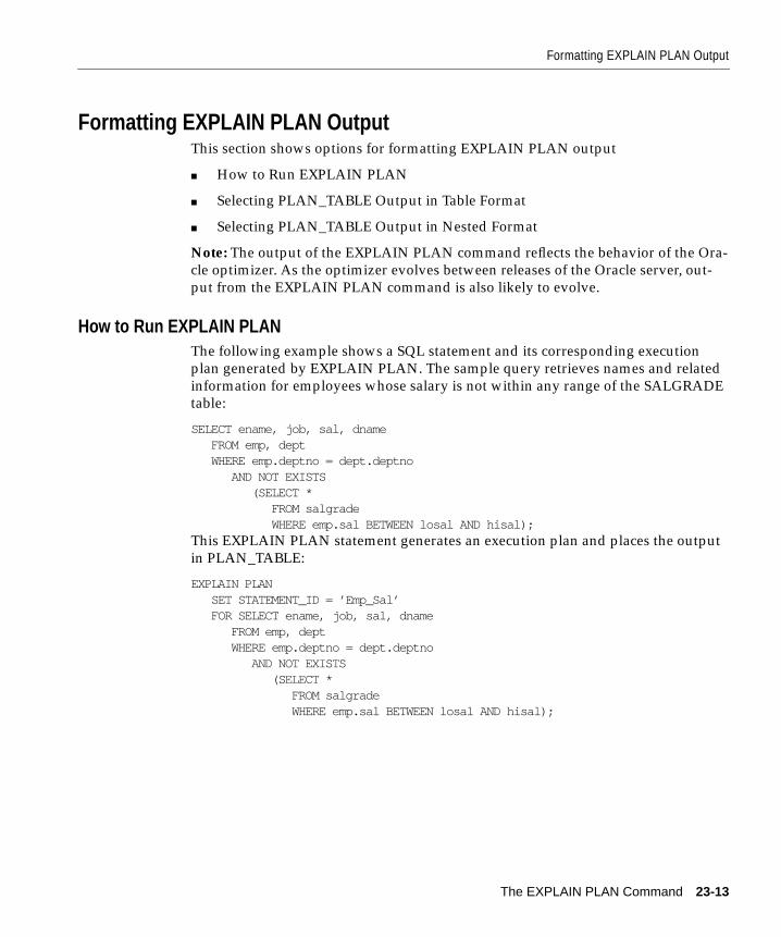
Formatting EXPLAIN PLAN Output
Formatting EXPLAIN PLAN OutputThis section shows options for formatting EXPLAIN PLAN output
■ How to Run EXPLAIN PLAN
■ Selecting PLAN_TABLE Output in Table Format
■ Selecting PLAN_TABLE Output in Nested Format
Note: The output of the EXPLAIN PLAN command reflects the behavior of the Ora-cle optimizer. As the optimizer evolves between releases of the Oracle server, out-put from the EXPLAIN PLAN command is also likely to evolve.
How to Run EXPLAIN PLANThe following example shows a SQL statement and its corresponding executionplan generated by EXPLAIN PLAN. The sample query retrieves names and relatedinformation for employees whose salary is not within any range of the SALGRADEtable:
SELECT ename, job, sal, dname FROM emp, dept WHERE emp.deptno = dept.deptno AND NOT EXISTS (SELECT * FROM salgrade WHERE emp.sal BETWEEN losal AND hisal);This EXPLAIN PLAN statement generates an execution plan and places the outputin PLAN_TABLE:
EXPLAIN PLAN SET STATEMENT_ID = ’Emp_Sal’ FOR SELECT ename, job, sal, dname FROM emp, dept WHERE emp.deptno = dept.deptno AND NOT EXISTS (SELECT * FROM salgrade WHERE emp.sal BETWEEN losal AND hisal);
The EXPLAIN PLAN Command 23-13
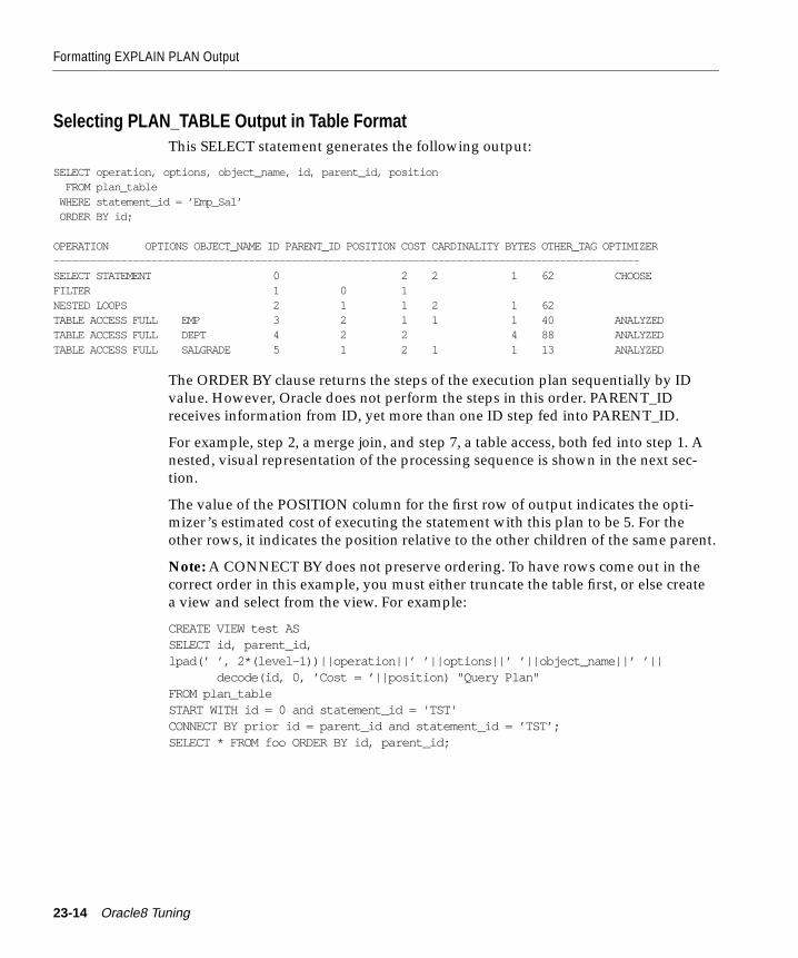
Formatting EXPLAIN PLAN Output
Selecting PLAN_TABLE Output in Table FormatThis SELECT statement generates the following output:
SELECT operation, options, object_name, id, parent_id, position FROM plan_table WHERE statement_id = ’Emp_Sal’ ORDER BY id;
OPERATION OPTIONS OBJECT_NAME ID PARENT_ID POSITION COST CARDINALITY BYTES OTHER_TAG OPTIMIZER------------------------------------------------------------------------------------------------SELECT STATEMENT 0 2 2 1 62 CHOOSEFILTER 1 0 1NESTED LOOPS 2 1 1 2 1 62TABLE ACCESS FULL EMP 3 2 1 1 1 40 ANALYZEDTABLE ACCESS FULL DEPT 4 2 2 4 88 ANALYZEDTABLE ACCESS FULL SALGRADE 5 1 2 1 1 13 ANALYZED
The ORDER BY clause returns the steps of the execution plan sequentially by IDvalue. However, Oracle does not perform the steps in this order. PARENT_IDreceives information from ID, yet more than one ID step fed into PARENT_ID.
For example, step 2, a merge join, and step 7, a table access, both fed into step 1. Anested, visual representation of the processing sequence is shown in the next sec-tion.
The value of the POSITION column for the first row of output indicates the opti-mizer’s estimated cost of executing the statement with this plan to be 5. For theother rows, it indicates the position relative to the other children of the same parent.
Note: A CONNECT BY does not preserve ordering. To have rows come out in thecorrect order in this example, you must either truncate the table first, or else createa view and select from the view. For example:
CREATE VIEW test ASSELECT id, parent_id,lpad(’ ’, 2*(level-1))||operation||’ ’||options||’ ’||object_name||’ ’|| decode(id, 0, ’Cost = ’||position) "Query Plan"FROM plan_tableSTART WITH id = 0 and statement_id = 'TST'CONNECT BY prior id = parent_id and statement_id = ’TST’;SELECT * FROM foo ORDER BY id, parent_id;
23-14 Oracle8 Tuning
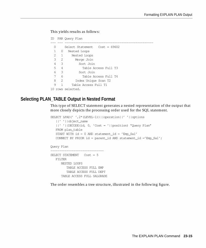
Formatting EXPLAIN PLAN Output
This yields results as follows:
ID PAR Query Plan--- --- -------------------------------------------------- 0 Select Statement Cost = 69602 1 0 Nested Loops 2 1 Nested Loops 3 2 Merge Join 4 3 Sort Join 5 4 Table Access Full T3 6 3 Sort Join 7 6 Table Access Full T4 8 2 Index Unique Scan T2 9 1 Table Access Full T110 rows selected.
Selecting PLAN_TABLE Output in Nested FormatThis type of SELECT statement generates a nested representation of the output thatmore closely depicts the processing order used for the SQL statement.
SELECT LPAD(’ ’,2*(LEVEL-1))||operation||’ ’||options ||’ ’||object_name ||’ ’||DECODE(id, 0, ’Cost = ’||position) ”Query Plan” FROM plan_table START WITH id = 0 AND statement_id = ’Emp_Sal’ CONNECT BY PRIOR id = parent_id AND statement_id =’Emp_Sal’;
Query Plan------------------------------SELECT STATEMENT Cost = 5 FILTER NESTED LOOPS TABLE ACCESS FULL EMP TABLE ACCESS FULL DEPT TABLE ACCESS FULL SALGRADE
The order resembles a tree structure, illustrated in the following figure.
The EXPLAIN PLAN Command 23-15
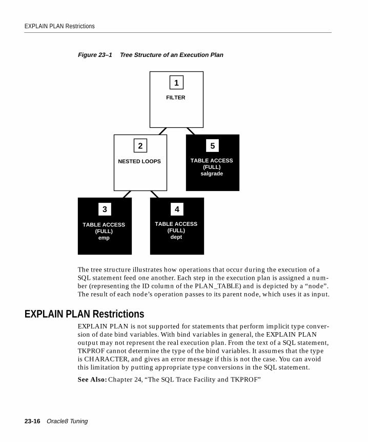
EXPLAIN PLAN Restrictions
Figure 23–1 Tree Structure of an Execution Plan
The tree structure illustrates how operations that occur during the execution of aSQL statement feed one another. Each step in the execution plan is assigned a num-ber (representing the ID column of the PLAN_TABLE) and is depicted by a “node”.The result of each node’s operation passes to its parent node, which uses it as input.
EXPLAIN PLAN RestrictionsEXPLAIN PLAN is not supported for statements that perform implicit type conver-sion of date bind variables. With bind variables in general, the EXPLAIN PLANoutput may not represent the real execution plan. From the text of a SQL statement,TKPROF cannot determine the type of the bind variables. It assumes that the typeis CHARACTER, and gives an error message if this is not the case. You can avoidthis limitation by putting appropriate type conversions in the SQL statement.
See Also: Chapter 24, “The SQL Trace Facility and TKPROF”
TABLE ACCESS(FULL)
emp
3 4
TABLE ACCESS(FULL)
dept
NESTED LOOPS
2 5
TABLE ACCESS(FULL)
salgrade
1
FILTER
23-16 Oracle8 Tuning
The SQL Trace Facility and TK
24
The SQL Trace Facility and TKPROFThe SQL trace facility and TKPROF are two basic performance diagnostic tools thatcan help you monitor and tune applications running against the Oracle Server. Thischapter covers:
■ Introduction
■ Step 1: Set Initialization Parameters for Trace File Management
■ Step 2: Enable the SQL Trace Facility
■ Step 3: Format Trace Files with TKPROF
■ Step 4: Interpret TKPROF Output
■ Step 5: Store SQL Trace Facility Statistics
■ Avoiding Pitfalls in TKPROF Interpretation
■ TKPROF Output Example
Note: The SQL trace facility and TKPROF program are subject to change in futurereleases of the Oracle Server. Such changes will be documented as they arise.
PROF 24-1
Introduction
IntroductionThe SQL trace facility and TKPROF enable you to accurately assess the efficiency ofthe SQL statements your application runs. For best results, use these tools withEXPLAIN PLAN, rather than using EXPLAIN PLAN alone. This section covers:
■ About the SQL Trace Facility
■ About TKPROF
■ How to Use the SQL Trace Facility and TKPROF
About the SQL Trace FacilityThe SQL trace facility provides performance information on individual SQL state-ments. It generates the following statistics for each statement:
■ Parse, execute, and fetch counts
■ CPU and elapsed times
■ Physical reads and logical reads
■ Number of rows processed
■ Misses on the library cache
■ Username under which each parse occurred
■ Each commit and rollback
You can enable the SQL trace facility for a session or for an instance. When the SQLtrace facility is enabled, performance statistics for all SQL statements executed in auser session or in an instance are placed into a trace file.
The additional overhead of running the SQL trace facility against an applicationwith performance problems is normally insignificant, compared with the inherentoverhead caused by the application’s inefficiency.
24-2 Oracle8 Tuning
Introduction
About TKPROFYou can run the TKPROF program to format the contents of the trace file and placethe output into a readable output file. Optionally, TKPROF can also
■ determine the execution plans of SQL statements
■ create a SQL script that stores the statistics in the database
S TKPROF reports each statement executed with the resources it has consumed, thenumber of times it was called, and the number of rows which it processed. Thisinformation lets you easily locate those statements that are using the greatestresource. With experience or with baselines available, you can assess whether theresources used are reasonable given the work done.
How to Use the SQL Trace Facility and TKPROFFollow these steps to use the SQL trace facility and TKPROF:
1. Set initialization parameters for trace file management.
2. Enable the SQL trace facility for the desired session and run your application.This step produces a trace file containing statistics for the SQL statementsissued by the application.
3. Run TKPROF to translate the trace file created in Step 2 into a readable outputfile. This step can optionally create a SQL script that stores the statistics in thedatabase.
4. Interpret the output file created in Step 3.
5. Optionally, run the SQL script produced in Step 3 to store the statistics in thedatabase.
In the following sections each of these steps is discussed in depth.
The SQL Trace Facility and TKPROF 24-3
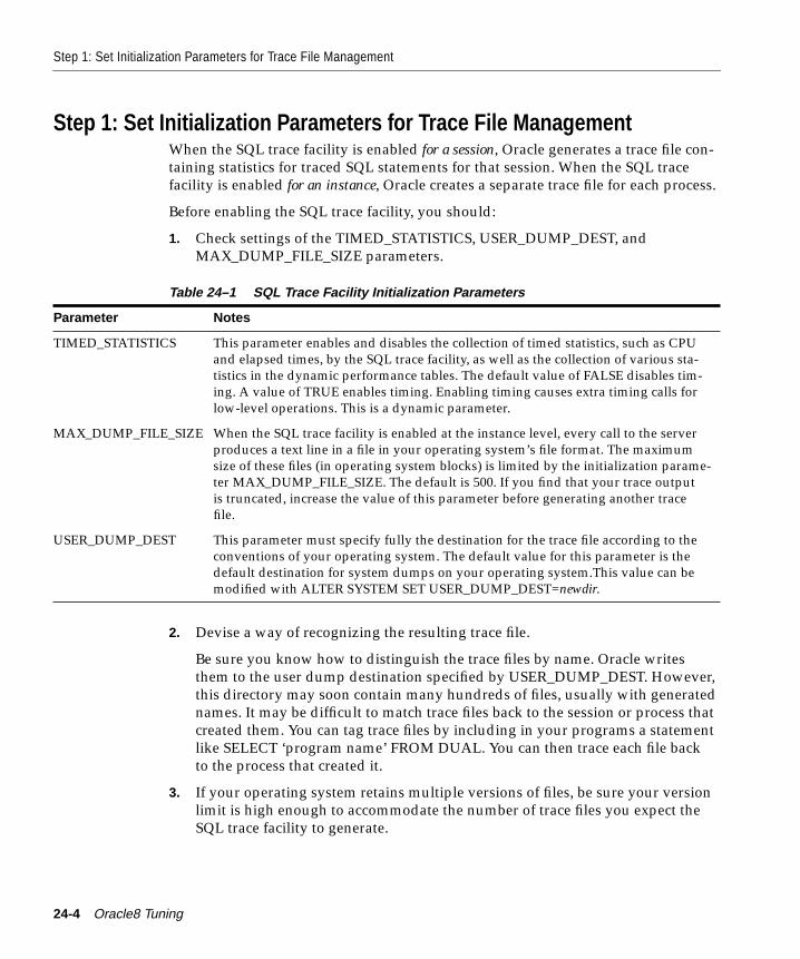
Step 1: Set Initialization Parameters for Trace File Management
Step 1: Set Initialization Parameters for Trace File ManagementWhen the SQL trace facility is enabled for a session, Oracle generates a trace file con-taining statistics for traced SQL statements for that session. When the SQL tracefacility is enabled for an instance, Oracle creates a separate trace file for each process.
Before enabling the SQL trace facility, you should:
1. Check settings of the TIMED_STATISTICS, USER_DUMP_DEST, andMAX_DUMP_FILE_SIZE parameters.
2. Devise a way of recognizing the resulting trace file.
Be sure you know how to distinguish the trace files by name. Oracle writesthem to the user dump destination specified by USER_DUMP_DEST. However,this directory may soon contain many hundreds of files, usually with generatednames. It may be difficult to match trace files back to the session or process thatcreated them. You can tag trace files by including in your programs a statementlike SELECT ‘program name’ FROM DUAL. You can then trace each file backto the process that created it.
3. If your operating system retains multiple versions of files, be sure your versionlimit is high enough to accommodate the number of trace files you expect theSQL trace facility to generate.
Table 24–1 SQL Trace Facility Initialization Parameters
Parameter Notes
TIMED_STATISTICS This parameter enables and disables the collection of timed statistics, such as CPUand elapsed times, by the SQL trace facility, as well as the collection of various sta-tistics in the dynamic performance tables. The default value of FALSE disables tim-ing. A value of TRUE enables timing. Enabling timing causes extra timing calls forlow-level operations. This is a dynamic parameter.
MAX_DUMP_FILE_SIZE When the SQL trace facility is enabled at the instance level, every call to the serverproduces a text line in a file in your operating system’s file format. The maximumsize of these files (in operating system blocks) is limited by the initialization parame-ter MAX_DUMP_FILE_SIZE. The default is 500. If you find that your trace outputis truncated, increase the value of this parameter before generating another tracefile.
USER_DUMP_DEST This parameter must specify fully the destination for the trace file according to theconventions of your operating system. The default value for this parameter is thedefault destination for system dumps on your operating system.This value can bemodified with ALTER SYSTEM SET USER_DUMP_DEST=newdir.
24-4 Oracle8 Tuning
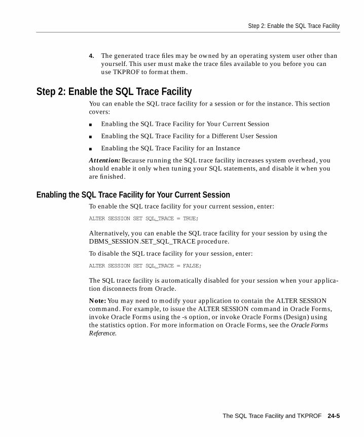
Step 2: Enable the SQL Trace Facility
4. The generated trace files may be owned by an operating system user other thanyourself. This user must make the trace files available to you before you canuse TKPROF to format them.
Step 2: Enable the SQL Trace FacilityYou can enable the SQL trace facility for a session or for the instance. This sectioncovers:
■ Enabling the SQL Trace Facility for Your Current Session
■ Enabling the SQL Trace Facility for a Different User Session
■ Enabling the SQL Trace Facility for an Instance
Attention: Because running the SQL trace facility increases system overhead, youshould enable it only when tuning your SQL statements, and disable it when youare finished.
Enabling the SQL Trace Facility for Your Current SessionTo enable the SQL trace facility for your current session, enter:
ALTER SESSION SET SQL_TRACE = TRUE;
Alternatively, you can enable the SQL trace facility for your session by using theDBMS_SESSION.SET_SQL_TRACE procedure.
To disable the SQL trace facility for your session, enter:
ALTER SESSION SET SQL_TRACE = FALSE;
The SQL trace facility is automatically disabled for your session when your applica-tion disconnects from Oracle.
Note: You may need to modify your application to contain the ALTER SESSIONcommand. For example, to issue the ALTER SESSION command in Oracle Forms,invoke Oracle Forms using the -s option, or invoke Oracle Forms (Design) usingthe statistics option. For more information on Oracle Forms, see the Oracle FormsReference.
The SQL Trace Facility and TKPROF 24-5
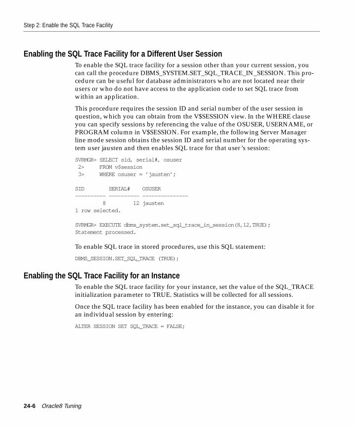
Step 2: Enable the SQL Trace Facility
Enabling the SQL Trace Facility for a Different User SessionTo enable the SQL trace facility for a session other than your current session, youcan call the procedure DBMS_SYSTEM.SET_SQL_TRACE_IN_SESSION. This pro-cedure can be useful for database administrators who are not located near theirusers or who do not have access to the application code to set SQL trace fromwithin an application.
This procedure requires the session ID and serial number of the user session inquestion, which you can obtain from the V$SESSION view. In the WHERE clauseyou can specify sessions by referencing the value of the OSUSER, USERNAME, orPROGRAM column in V$SESSION. For example, the following Server Managerline mode session obtains the session ID and serial number for the operating sys-tem user jausten and then enables SQL trace for that user’s session:
SVRMGR> SELECT sid, serial#, osuser 2> FROM v$session 3> WHERE osuser = ’jausten’;
SID SERIAL# OSUSER---------- ---------- --------------- 8 12 jausten1 row selected.
SVRMGR> EXECUTE dbms_system.set_sql_trace_in_session(8,12,TRUE);Statement processed.
To enable SQL trace in stored procedures, use this SQL statement:
DBMS_SESSION.SET_SQL_TRACE (TRUE);
Enabling the SQL Trace Facility for an InstanceTo enable the SQL trace facility for your instance, set the value of the SQL_TRACEinitialization parameter to TRUE. Statistics will be collected for all sessions.
Once the SQL trace facility has been enabled for the instance, you can disable it foran individual session by entering:
ALTER SESSION SET SQL_TRACE = FALSE;
24-6 Oracle8 Tuning
Step 3: Format Trace Files with TKPROF
Step 3: Format Trace Files with TKPROFThis section covers:
■ Sample TKPROF Output
■ Syntax of TKPROF
■ TKPROF Statement Examples
TKPROF accepts as input a trace file produced by the SQL trace facility and pro-duces a formatted output file. TKPROF can also be used to generate executionplans.
Once the SQL trace facility has generated a number of trace files, you can:
■ Run TKPROF on each individual trace file, producing a number of formattedoutput files, one for each session
■ Concatenate the trace files and then run TKPROF on the result to produce a for-matted output file for the entire instance
TKPROF does not report COMMITs and ROLLBACKs that are recorded in the tracefile.
The SQL Trace Facility and TKPROF 24-7
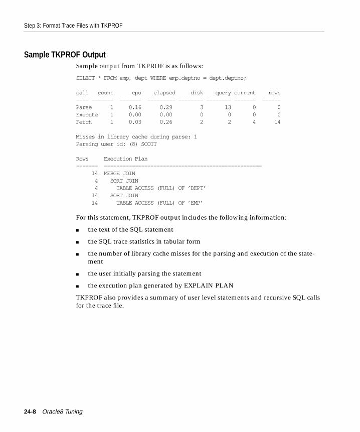
Step 3: Format Trace Files with TKPROF
Sample TKPROF OutputSample output from TKPROF is as follows:
SELECT * FROM emp, dept WHERE emp.deptno = dept.deptno;
call count cpu elapsed disk query current rows---- ------- ------- --------- -------- -------- ------- ------Parse 1 0.16 0.29 3 13 0 0Execute 1 0.00 0.00 0 0 0 0Fetch 1 0.03 0.26 2 2 4 14
Misses in library cache during parse: 1Parsing user id: (8) SCOTT
Rows Execution Plan------- --------------------------------------------------- 14 MERGE JOIN 4 SORT JOIN 4 TABLE ACCESS (FULL) OF ’DEPT’ 14 SORT JOIN 14 TABLE ACCESS (FULL) OF ’EMP’
For this statement, TKPROF output includes the following information:
■ the text of the SQL statement
■ the SQL trace statistics in tabular form
■ the number of library cache misses for the parsing and execution of the state-ment
■ the user initially parsing the statement
■ the execution plan generated by EXPLAIN PLAN
TKPROF also provides a summary of user level statements and recursive SQL callsfor the trace file.
24-8 Oracle8 Tuning
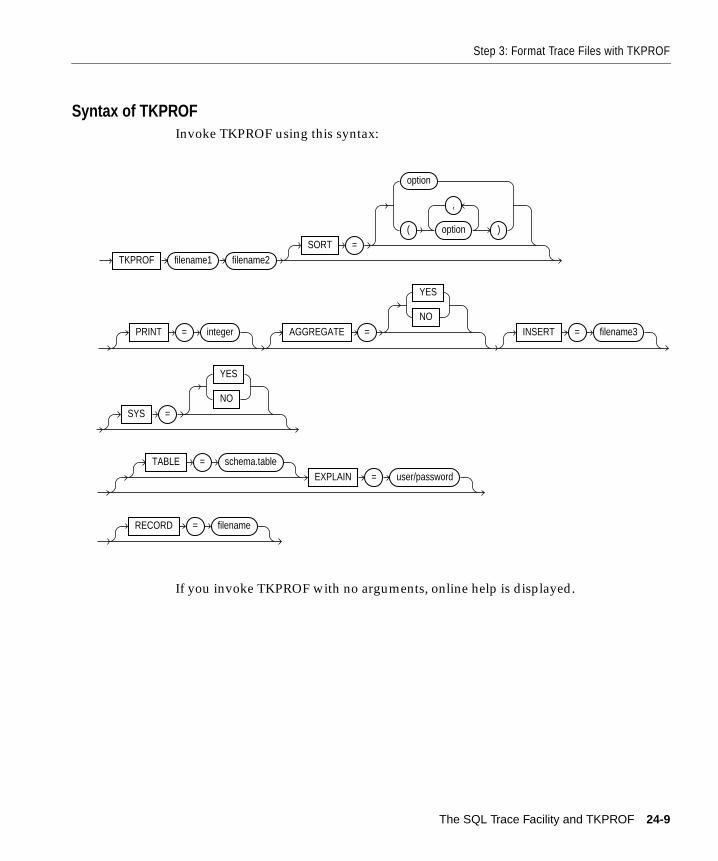
Step 3: Format Trace Files with TKPROF
Syntax of TKPROFInvoke TKPROF using this syntax:
If you invoke TKPROF with no arguments, online help is displayed.
TKPROF filename1 filename2SORT =
option
( option
,
)
tkprof_command
PRINT = integer AGGREGATE =
YES
NOINSERT = filename3
TABLE = schema.tableEXPLAIN = user/password
RECORD = filename
SYS =
YES
NO
The SQL Trace Facility and TKPROF 24-9
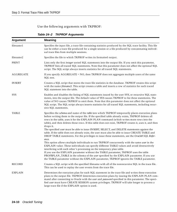
Step 3: Format Trace Files with TKPROF
Use the following arguments with TKPROF:
Table 24–2 TKPROF Arguments
Argument Meaning
filename1 Specifies the input file, a trace file containing statistics produced by the SQL trace facility. This filecan be either a trace file produced for a single session or a file produced by concatenating individ-ual trace files from multiple sessions.
filename2 Specifies the file to which TKPROF writes its formatted output.
PRINT Lists only the first integer sorted SQL statements into the output file. If you omit this parameter,TKPROF lists all traced SQL statements. Note that this parameter does not affect the optional SQLscript. The SQL script always inserts statistics for all traced SQL statements.
AGGREGATE If you specify AGGREGATE = NO, then TKPROF does not aggregate multiple users of the sameSQL text.
INSERT Creates a SQL script that stores the trace file statistics in the database. TKPROF creates this scriptwith the name filename3. This script creates a table and inserts a row of statistics for each tracedSQL statement into the table.
SYS Enables and disables the listing of SQL statements issued by the user SYS, or recursive SQL state-ments, into the output file. The default value of YES causes TKPROF to list these statements. Thevalue of NO causes TKPROF to omit them. Note that this parameter does not affect the optionalSQL script. The SQL script always inserts statistics for all traced SQL statements, including recur-sive SQL statements.
TABLE Specifies the schema and name of the table into which TKPROF temporarily places execution plansbefore writing them to the output file. If the specified table already exists, TKPROF deletes allrows in the table, uses it for the EXPLAIN PLAN command (which writes more rows into thetable), and then deletes those rows. If this table does not exist, TKPROF creates it, uses it, and thendrops it.The specified user must be able to issue INSERT, SELECT, and DELETE statements against thetable. If the table does not already exist, the user must also be able to issue CREATE TABLE andDROP TABLE statements. For the privileges to issue these statements, see the Oracle8 SQL Refer-ence.This option allows multiple individuals to run TKPROF concurrently with the same user in theEXPLAIN value. These individuals can specify different TABLE values and avoid destructivelyinterfering with each other’s processing on the temporary plan table.If you use the EXPLAIN parameter without the TABLE parameter, TKPROF uses the tablePROF$PLAN_TABLE in the schema of the user specified by the EXPLAIN parameter. If you usethe TABLE parameter without the EXPLAIN parameter, TKPROF ignores the TABLE parameter.
RECORD Creates a SQL script with the specified filename with all of the nonrecursive SQL in the trace file.This can be used to replay the user events from the trace file.
EXPLAIN Determines the execution plan for each SQL statement in the trace file and writes these executionplans to the output file. TKPROF determines execution plans by issuing the EXPLAIN PLAN com-mand after connecting to Oracle with the user and password specified in this parameter. The speci-fied user must have CREATE SESSION system privileges. TKPROF will take longer to process alarge trace file if the EXPLAIN option is used.
24-10 Oracle8 Tuning
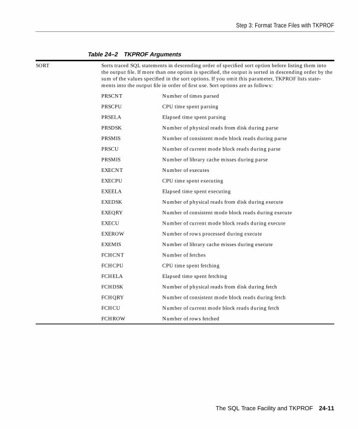
Step 3: Format Trace Files with TKPROF
SORT Sorts traced SQL statements in descending order of specified sort option before listing them intothe output file. If more than one option is specified, the output is sorted in descending order by thesum of the values specified in the sort options. If you omit this parameter, TKPROF lists state-ments into the output file in order of first use. Sort options are as follows:
PRSCNT Number of times parsed
PRSCPU CPU time spent parsing
PRSELA Elapsed time spent parsing
PRSDSK Number of physical reads from disk during parse
PRSMIS Number of consistent mode block reads during parse
PRSCU Number of current mode block reads during parse
PRSMIS Number of library cache misses during parse
EXECNT Number of executes
EXECPU CPU time spent executing
EXEELA Elapsed time spent executing
EXEDSK Number of physical reads from disk during execute
EXEQRY Number of consistent mode block reads during execute
EXECU Number of current mode block reads during execute
EXEROW Number of rows processed during execute
EXEMIS Number of library cache misses during execute
FCHCNT Number of fetches
FCHCPU CPU time spent fetching
FCHELA Elapsed time spent fetching
FCHDSK Number of physical reads from disk during fetch
FCHQRY Number of consistent mode block reads during fetch
FCHCU Number of current mode block reads during fetch
FCHROW Number of rows fetched
Table 24–2 TKPROF Arguments
The SQL Trace Facility and TKPROF 24-11
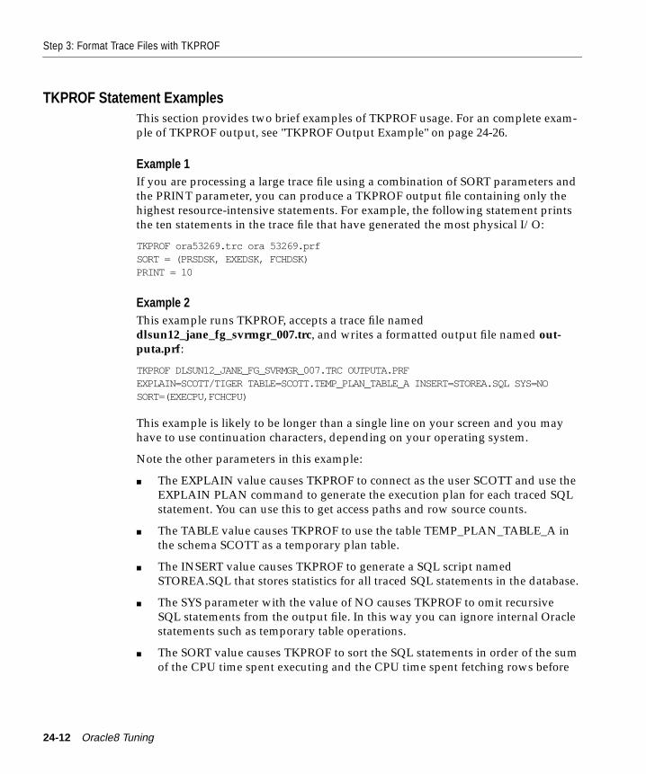
Step 3: Format Trace Files with TKPROF
TKPROF Statement ExamplesThis section provides two brief examples of TKPROF usage. For an complete exam-ple of TKPROF output, see "TKPROF Output Example" on page 24-26.
Example 1If you are processing a large trace file using a combination of SORT parameters andthe PRINT parameter, you can produce a TKPROF output file containing only thehighest resource-intensive statements. For example, the following statement printsthe ten statements in the trace file that have generated the most physical I/O:
TKPROF ora53269.trc ora 53269.prfSORT = (PRSDSK, EXEDSK, FCHDSK)PRINT = 10
Example 2This example runs TKPROF, accepts a trace file nameddlsun12_jane_fg_svrmgr_007.trc, and writes a formatted output file named out-puta.prf:
TKPROF DLSUN12_JANE_FG_SVRMGR_007.TRC OUTPUTA.PRFEXPLAIN=SCOTT/TIGER TABLE=SCOTT.TEMP_PLAN_TABLE_A INSERT=STOREA.SQL SYS=NOSORT=(EXECPU,FCHCPU)
This example is likely to be longer than a single line on your screen and you mayhave to use continuation characters, depending on your operating system.
Note the other parameters in this example:
■ The EXPLAIN value causes TKPROF to connect as the user SCOTT and use theEXPLAIN PLAN command to generate the execution plan for each traced SQLstatement. You can use this to get access paths and row source counts.
■ The TABLE value causes TKPROF to use the table TEMP_PLAN_TABLE_A inthe schema SCOTT as a temporary plan table.
■ The INSERT value causes TKPROF to generate a SQL script namedSTOREA.SQL that stores statistics for all traced SQL statements in the database.
■ The SYS parameter with the value of NO causes TKPROF to omit recursiveSQL statements from the output file. In this way you can ignore internal Oraclestatements such as temporary table operations.
■ The SORT value causes TKPROF to sort the SQL statements in order of the sumof the CPU time spent executing and the CPU time spent fetching rows before
24-12 Oracle8 Tuning
Step 4: Interpret TKPROF Output
writing them to the output file. For greatest efficiency, always use SORT param-eters.
Step 4: Interpret TKPROF OutputThis section provides pointers for interpreting TKPROF output.
■ Tabular Statistics
■ Library Cache Misses
■ Statement Truncation
■ User Issuing the SQL Statement
■ Execution Plan
■ Deciding Which Statements to Tune
While TKPROF provides a very useful analysis, the most accurate measure of effi-ciency is the actual performance of the application in question. Note that at the endof the TKPROF output is a summary of the work done in the database engine bythe process during the period that the trace was running.
See Also: Oracle8 Reference for a description of statistics in V$SYSSTAT andV$SESSTAT.
Tabular StatisticsTKPROF lists the statistics for a SQL statement returned by the SQL trace facility inrows and columns. Each row corresponds to one of three steps of SQL statementprocessing. The step for which each row contains statistics is identified by the valueof the CALL column:
PARSE This step translates the SQL statement into an executionplan. This step includes checks for proper security authoriza-tion and checks for the existence of tables, columns, andother referenced objects.
EXECUTE This step is the actual execution of the statement by Oracle.For INSERT, UPDATE, and DELETE statements, this stepmodifies the data. For SELECT statements, the step identifiesthe selected rows.
FETCH This step retrieves rows returned by a query. Fetches areonly performed for SELECT statements.
The SQL Trace Facility and TKPROF 24-13
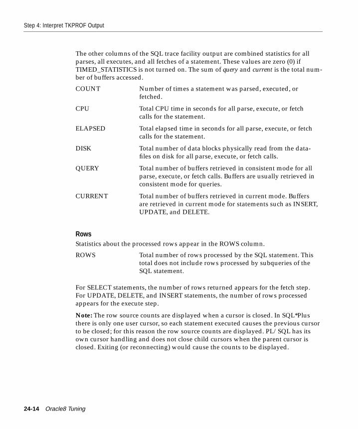
Step 4: Interpret TKPROF Output
The other columns of the SQL trace facility output are combined statistics for allparses, all executes, and all fetches of a statement. These values are zero (0) ifTIMED_STATISTICS is not turned on. The sum of query and current is the total num-ber of buffers accessed.
RowsStatistics about the processed rows appear in the ROWS column.
For SELECT statements, the number of rows returned appears for the fetch step.For UPDATE, DELETE, and INSERT statements, the number of rows processedappears for the execute step.
Note: The row source counts are displayed when a cursor is closed. In SQL*Plusthere is only one user cursor, so each statement executed causes the previous cursorto be closed; for this reason the row source counts are displayed. PL/SQL has itsown cursor handling and does not close child cursors when the parent cursor isclosed. Exiting (or reconnecting) would cause the counts to be displayed.
COUNT Number of times a statement was parsed, executed, orfetched.
CPU Total CPU time in seconds for all parse, execute, or fetchcalls for the statement.
ELAPSED Total elapsed time in seconds for all parse, execute, or fetchcalls for the statement.
DISK Total number of data blocks physically read from the data-files on disk for all parse, execute, or fetch calls.
QUERY Total number of buffers retrieved in consistent mode for allparse, execute, or fetch calls. Buffers are usually retrieved inconsistent mode for queries.
CURRENT Total number of buffers retrieved in current mode. Buffersare retrieved in current mode for statements such as INSERT,UPDATE, and DELETE.
ROWS Total number of rows processed by the SQL statement. Thistotal does not include rows processed by subqueries of theSQL statement.
24-14 Oracle8 Tuning
Step 4: Interpret TKPROF Output
Resolution of StatisticsTiming statistics have a resolution of one hundredth of a second; therefore, anyoperation on a cursor that takes a hundredth of a second or less may not be timedaccurately. Keep this in mind when interpreting statistics. In particular, be carefulwhen interpreting the results from simple queries that execute very quickly.
Recursive CallsSometimes in order to execute a SQL statement issued by a user, Oracle must issueadditional statements. Such statements are called recursive calls or recursive SQLstatements. For example, if you insert a row into a table that does not have enoughspace to hold that row, Oracle makes recursive calls to allocate the space dynami-cally. Recursive calls are also generated when data dictionary information is notavailable in the data dictionary cache and must be retrieved from disk.
If recursive calls occur while the SQL trace facility is enabled, TKPROF producesstatistics for the recursive SQL statements and marks them clearly as recursive SQLstatements in the output file. You can suppress the listing of recursive calls in theoutput file by setting the SYS command-line parameter to NO. Note that the statis-tics for a recursive SQL statement are included in the listing for that statement, notin the listing for the SQL statement that caused the recursive call. So when you arecalculating the total resources required to process a SQL statement, you should con-sider the statistics for that statement as well as those for recursive calls caused bythat statement.
Library Cache MissesTKPROF also lists the number of library cache misses resulting from parse and exe-cute steps for each SQL statement. These statistics appear on separate lines follow-ing the tabular statistics. If the statement resulted in no library cache misses,TKPROF does not list the statistic. In "Sample TKPROF Output" on page 24-8, theexample, the statement resulted in one library cache miss for the parse step and nomisses for the execute step.
The SQL Trace Facility and TKPROF 24-15
Step 4: Interpret TKPROF Output
Statement TruncationThe following SQL statements are truncated to 25 characters in the SQL trace file:
SET ROLEGRANTALTER USERALTER ROLECREATE USERCREATE ROLE
User Issuing the SQL StatementTKPROF also lists the user ID of the user issuing each SQL statement. If the SQLtrace input file contained statistics from multiple users and the statement wasissued by more than one user, TKPROF lists the ID of the last user to parse the state-ment. The user ID of all database users appears in the data dictionary in the col-umn ALL_USERS.USER_ID.
Execution PlanIf you specify the EXPLAIN parameter on the TKPROF command line, TKPROFuses the EXPLAIN PLAN command to generate the execution plan of each SQLstatement traced. TKPROF also displays the number of rows processed by eachstep of the execution plan.
Note: Trace files generated immediately after instance startup contain data thatreflects the activity of the startup process. In particular, they reflect a disproportion-ate amount of I/O activity as caches in the system global area (SGA) are filled. Forthe purposes of tuning, ignore such trace files.
See Also: Chapter 23, “The EXPLAIN PLAN Command” for more information oninterpreting execution plans.
24-16 Oracle8 Tuning
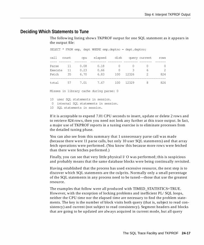
Step 4: Interpret TKPROF Output
Deciding Which Statements to TuneThe following listing shows TKPROF output for one SQL statement as it appears inthe output file:
SELECT * FROM emp, dept WHERE emp.deptno = dept.deptno;
call count cpu elapsed disk query current rows---- ------- ------- --------- -------- -------- ------- ------Parse 11 0.08 0.18 0 0 0 0Execute 11 0.23 0.66 0 3 6 2Fetch 35 6.70 6.83 100 12326 2 824------------------------------------------------------------------total 57 7.01 7.67 100 12329 8 826
Misses in library cache during parse: 0
10 user SQL statements in session. 0 internal SQL statements in session.10 SQL statements in session.
If it is acceptable to expend 7.01 CPU seconds to insert, update or delete 2 rows andto retrieve 824 rows, then you need not look any further at this trace output. In fact,a major use of TKPROF reports in a tuning exercise is to eliminate processes fromthe detailed tuning phase.
You can also see from this summary that 1 unnecessary parse call was made(because there were 11 parse calls, but only 10 user SQL statements) and that arrayfetch operations were performed. (You know this because more rows were fetchedthan there were fetches performed.)
Finally, you can see that very little physical I/O was performed; this is suspiciousand probably means that the same database blocks were being continually revisited.
Having established that the process has used excessive resource, the next step is todiscover which SQL statements are the culprits. Normally only a small percentageof the SQL statements in any process need to be tuned—those that use the greatestresource.
The examples that follow were all produced with TIMED_STATISTICS=TRUE.However, with the exception of locking problems and inefficient PL/SQL loops,neither the CPU time nor the elapsed time are necessary to find the problem state-ments. The key is the number of block visits both query (that is, subject to read con-sistency) and current (not subject to read consistency). Segment headers and blocksthat are going to be updated are always acquired in current mode, but all query
The SQL Trace Facility and TKPROF 24-17
Step 5: Store SQL Trace Facility Statistics
and subquery processing requests the data in query mode. These are precisely thesame measures as the instance statistics CONSISTENT GETS and DB BLOCK GETS.
The SQL parsed as SYS is recursive SQL used to maintain the dictionary cache, andis not normally of great benefit. If the number of internal SQL statements lookshigh, you might want to check to see what has been going on. (There may be exces-sive space management overhead.)
Step 5: Store SQL Trace Facility StatisticsThis section covers:
■ Generating the TKPROF Output SQL Script
■ Editing the TKPROF Output SQL Script
■ Querying the Output Table
You may want to keep a history of the statistics generated by the SQL trace facilityfor your application and compare them over time. TKPROF can generate a SQLscript that creates a table and inserts rows of statistics into it. This script contains
■ a CREATE TABLE statement that creates an output table namedTKPROF_TABLE
■ INSERT statements that add rows of statistics, one for each traced SQL state-ment, to the TKPROF_TABLE
After running TKPROF, you can run this script to store the statistics in the database.
Generating the TKPROF Output SQL ScriptWhen you run TKPROF, use the INSERT parameter to specify the name of the gen-erated SQL script. If you omit this parameter, TKPROF does not generate a script.
Editing the TKPROF Output SQL ScriptAfter TKPROF has created the SQL script, you may want to edit the script beforerunning it.
If you have already created an output table for previously collected statistics andyou want to add new statistics to this table, remove the CREATE TABLE statementfrom the script. The script will then insert the new rows into the existing table.
If you have created multiple output tables, perhaps to store statistics from differentdatabases in different tables, edit the CREATE TABLE and INSERT statements tochange the name of the output table.
24-18 Oracle8 Tuning
Step 5: Store SQL Trace Facility Statistics
Querying the Output TableThe following CREATE TABLE statement creates the TKPROF_TABLE:
CREATE TABLE tkprof_table (date_of_insert DATE, cursor_num NUMBER, depth NUMBER, user_id NUMBER, parse_cnt NUMBER, parse_cpu NUMBER, parse_elap NUMBER, parse_disk NUMBER, parse_query NUMBER, parse_current NUMBER, parse_miss NUMBER, exe_count NUMBER, exe_cpu NUMBER, exe_elap NUMBER, exe_disk NUMBER, exe_query NUMBER, exe_current NUMBER, exe_miss NUMBER, exe_rows NUMBER, fetch_count NUMBER, fetch_cpu NUMBER, fetch_elap NUMBER, fetch_disk NUMBER, fetch_query NUMBER, fetch_current NUMBER, fetch_rows NUMBER, clock_ticks NUMBER, sql_statement LONG);
Most output table columns correspond directly to the statistics that appear in theformatted output file. For example, the PARSE_CNT column value corresponds tothe count statistic for the parse step in the output file.
The SQL Trace Facility and TKPROF 24-19
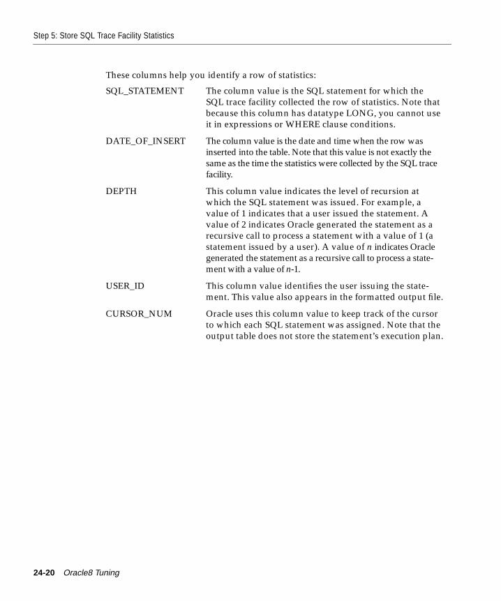
Step 5: Store SQL Trace Facility Statistics
These columns help you identify a row of statistics:
SQL_STATEMENT The column value is the SQL statement for which theSQL trace facility collected the row of statistics. Note thatbecause this column has datatype LONG, you cannot useit in expressions or WHERE clause conditions.
DATE_OF_INSERT The column value is the date and time when the row wasinserted into the table. Note that this value is not exactly thesame as the time the statistics were collected by the SQL tracefacility.
DEPTH This column value indicates the level of recursion atwhich the SQL statement was issued. For example, avalue of 1 indicates that a user issued the statement. Avalue of 2 indicates Oracle generated the statement as arecursive call to process a statement with a value of 1 (astatement issued by a user). A value of n indicates Oraclegenerated the statement as a recursive call to process a state-ment with a value of n-1.
USER_ID This column value identifies the user issuing the state-ment. This value also appears in the formatted output file.
CURSOR_NUM Oracle uses this column value to keep track of the cursorto which each SQL statement was assigned. Note that theoutput table does not store the statement’s execution plan.
24-20 Oracle8 Tuning
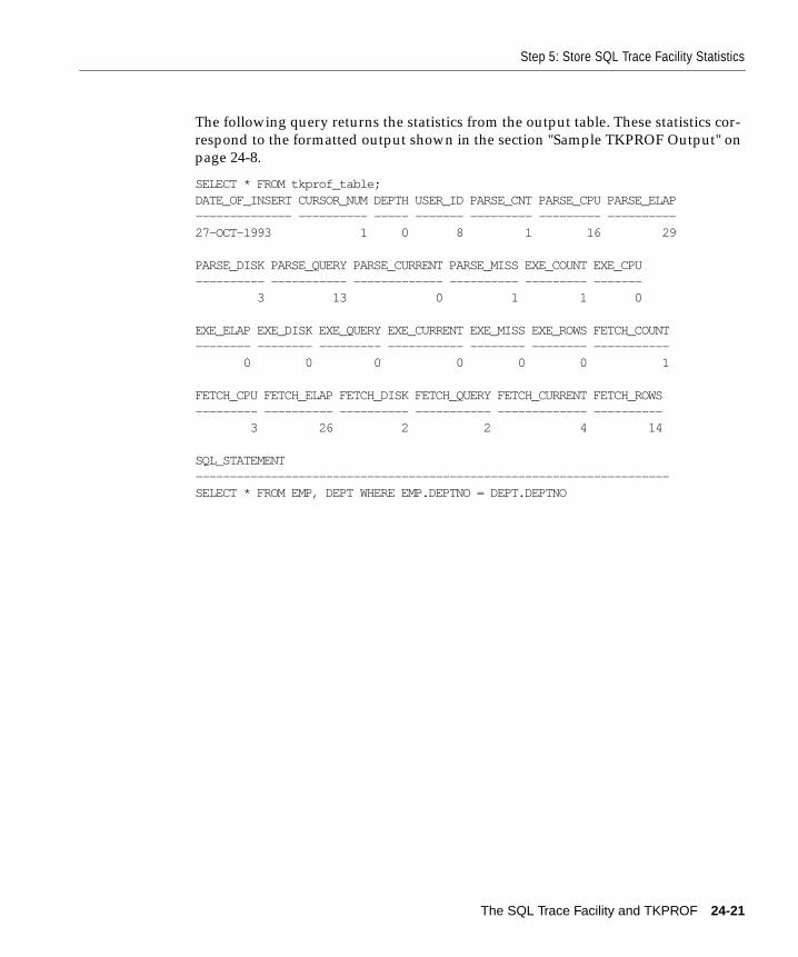
Step 5: Store SQL Trace Facility Statistics
The following query returns the statistics from the output table. These statistics cor-respond to the formatted output shown in the section "Sample TKPROF Output" onpage 24-8.
SELECT * FROM tkprof_table;DATE_OF_INSERT CURSOR_NUM DEPTH USER_ID PARSE_CNT PARSE_CPU PARSE_ELAP-------------- ---------- ----- ------- --------- --------- ----------27-OCT-1993 1 0 8 1 16 29
PARSE_DISK PARSE_QUERY PARSE_CURRENT PARSE_MISS EXE_COUNT EXE_CPU---------- ----------- ------------- ---------- --------- ------- 3 13 0 1 1 0
EXE_ELAP EXE_DISK EXE_QUERY EXE_CURRENT EXE_MISS EXE_ROWS FETCH_COUNT-------- -------- --------- ----------- -------- -------- ----------- 0 0 0 0 0 0 1
FETCH_CPU FETCH_ELAP FETCH_DISK FETCH_QUERY FETCH_CURRENT FETCH_ROWS--------- ---------- ---------- ----------- ------------- ---------- 3 26 2 2 4 14
SQL_STATEMENT---------------------------------------------------------------------SELECT * FROM EMP, DEPT WHERE EMP.DEPTNO = DEPT.DEPTNO
The SQL Trace Facility and TKPROF 24-21
Avoiding Pitfalls in TKPROF Interpretation
Avoiding Pitfalls in TKPROF InterpretationThis section describes some fine points of TKPROF interpretation:
■ Finding Which Statements Constitute the Bulk of the Load
■ The Argument Trap
■ The Read Consistency Trap
■ The Schema Trap
■ The Time Trap
■ The Trigger Trap
■ The “Correct” Version
See Also: "EXPLAIN PLAN Restrictions" on page 23-16 for information aboutTKPROF and bind variables.
Finding Which Statements Constitute the Bulk of the LoadLook at the totals and try to identify the statements that constitute the bulk of theload.
Do not attempt to perform many different jobs within a single query. It is moreeffective to separate out the different queries that should be used when particularoptional parameters are present, and when the parameters provided contain wildcards.
If particular parameters are not specified by the report user, the query uses bindvariables that have been set to “%”. This action has the effect of ignoring any LIKEclauses in the query. It would be more efficient to run a query in which theseclauses are not present.
Note: TKPROF cannot determine the TYPE of the bind variables from the text ofthe SQL statement. It assumes that TYPE is CHARACTER. If this is not the case,you should put appropriate type conversions in the SQL statement.
The Argument TrapIf you are not aware of the values being bound at run time, it is possible to fall intothe “argument trap”. Especially where the LIKE operator is used, the query may bemarkedly less efficient for particular values, or types of value, in a bind variable.This is because the optimizer must make an assumption about the probable selectiv-ity without knowing the value.
24-22 Oracle8 Tuning
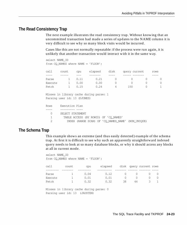
Avoiding Pitfalls in TKPROF Interpretation
The Read Consistency TrapThe next example illustrates the read consistency trap. Without knowing that anuncommitted transaction had made a series of updates to the NAME column it isvery difficult to see why so many block visits would be incurred.
Cases like this are not normally repeatable: if the process were run again, it isunlikely that another transaction would interact with it in the same way.
select NAME_IDfrom CQ_NAMES where NAME = ’FLOOR’;
call count cpu elapsed disk query current rows---- ----- --- ------- ---- ----- ------- ----Parse 1 0.11 0.21 0 0 0 0Execute 1 0.00 0.00 0 0 0 0Fetch 1 0.15 0.24 4 150 0 1
Misses in library cache during parse: 1Parsing user id: 13 (DJONES)
Rows Execution Plan---- --------- ---- 0 SELECT STATEMENT 1 TABLE ACCESS (BY ROWID) OF ’CQ_NAMES’ 2 INDEX (RANGE SCAN) OF ’CQ_NAMES_NAME’ (NON_UNIQUE)
The Schema TrapThis example shows an extreme (and thus easily detected) example of the schematrap. At first it is difficult to see why such an apparently straightforward indexedquery needs to look at so many database blocks, or why it should access any blocksat all in current mode.
select NAME_IDfrom CQ_NAMES where NAME = ’FLOOR’;
call count cpu elapsed disk query current rows-------- ------- -------- --------- ------- ------ ------- ----Parse 1 0.04 0.12 0 0 0 0Execute 1 0.01 0.01 0 0 0 0Fetch 1 0.32 0.32 38 44 3 1
Misses in library cache during parse: 0Parsing user id: 13 (JAUSTEN)
The SQL Trace Facility and TKPROF 24-23
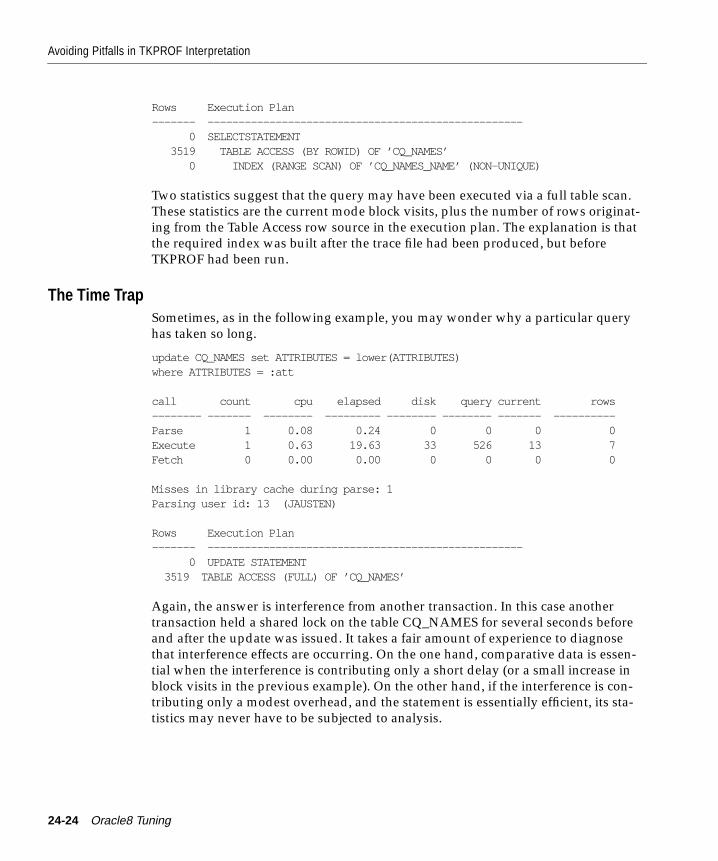
Avoiding Pitfalls in TKPROF Interpretation
Rows Execution Plan------- --------------------------------------------------- 0 SELECTSTATEMENT 3519 TABLE ACCESS (BY ROWID) OF ’CQ_NAMES’ 0 INDEX (RANGE SCAN) OF ’CQ_NAMES_NAME’ (NON-UNIQUE)
Two statistics suggest that the query may have been executed via a full table scan.These statistics are the current mode block visits, plus the number of rows originat-ing from the Table Access row source in the execution plan. The explanation is thatthe required index was built after the trace file had been produced, but beforeTKPROF had been run.
The Time TrapSometimes, as in the following example, you may wonder why a particular queryhas taken so long.
update CQ_NAMES set ATTRIBUTES = lower(ATTRIBUTES)where ATTRIBUTES = :att
call count cpu elapsed disk query current rows-------- ------- -------- --------- -------- -------- ------- ----------Parse 1 0.08 0.24 0 0 0 0Execute 1 0.63 19.63 33 526 13 7Fetch 0 0.00 0.00 0 0 0 0
Misses in library cache during parse: 1Parsing user id: 13 (JAUSTEN)
Rows Execution Plan------- --------------------------------------------------- 0 UPDATE STATEMENT 3519 TABLE ACCESS (FULL) OF ’CQ_NAMES’
Again, the answer is interference from another transaction. In this case anothertransaction held a shared lock on the table CQ_NAMES for several seconds beforeand after the update was issued. It takes a fair amount of experience to diagnosethat interference effects are occurring. On the one hand, comparative data is essen-tial when the interference is contributing only a short delay (or a small increase inblock visits in the previous example). On the other hand, if the interference is con-tributing only a modest overhead, and the statement is essentially efficient, its sta-tistics may never have to be subjected to analysis.
24-24 Oracle8 Tuning
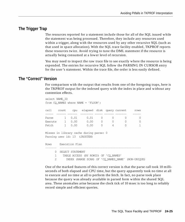
Avoiding Pitfalls in TKPROF Interpretation
The Trigger TrapThe resources reported for a statement include those for all of the SQL issued whilethe statement was being processed. Therefore, they include any resources usedwithin a trigger, along with the resources used by any other recursive SQL (such asthat used in space allocation). With the SQL trace facility enabled, TKPROF reportsthese resources twice. Avoid trying to tune the DML statement if the resource isactually being consumed at a lower level of recursion.
You may need to inspect the raw trace file to see exactly where the resource is beingexpended. The entries for recursive SQL follow the PARSING IN CURSOR entryfor the user’s statement. Within the trace file, the order is less easily defined.
The “Correct” VersionFor comparison with the output that results from one of the foregoing traps, here isthe TKPROF output for the indexed query with the index in place and without anycontention effects.
select NAME_IDfrom CQ_NAMES where NAME = ’FLOOR’;
call count cpu elapsed disk query current rows----- ------ ------ -------- ----- ------ ------- -----Parse 1 0.01 0.01 0 0 0 0Execute 1 0.00 0.00 0 0 0 0Fetch 1 0.00 0.00 0 4 0 1
Misses in library cache during parse: 0Parsing user id: 13 (JAUSTEN)
Rows Execution Plan------- --------------------------------------------------- 0 SELECT STATEMENT 1 TABLE ACCESS (BY ROWID) OF ’CQ_NAMES’ 2 INDEX (RANGE SCAN) OF ’CQ_NAMES_NAME’ (NON-UNIQUE)
One of the marked features of this correct version is that the parse call took 10 milli-seconds of both elapsed and CPU time, but the query apparently took no time at allto execute and no time at all to perform the fetch. In fact, no parse took placebecause the query was already available in parsed form within the shared SQLarea. These anomalies arise because the clock tick of 10 msec is too long to reliablyrecord simple and efficient queries.
The SQL Trace Facility and TKPROF 24-25
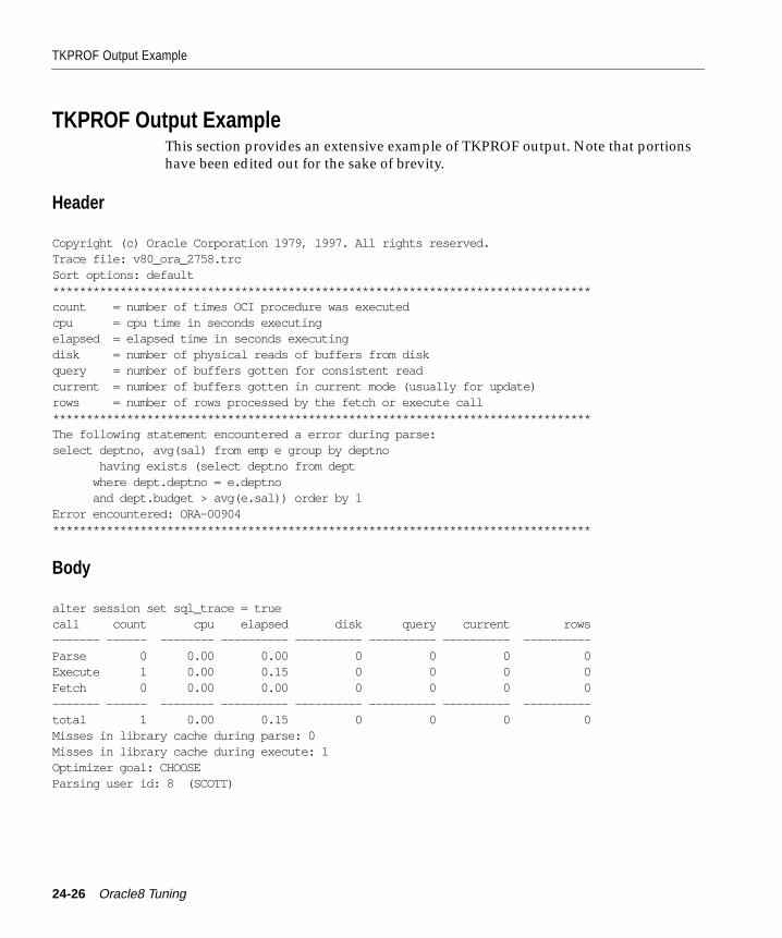
TKPROF Output Example
TKPROF Output ExampleThis section provides an extensive example of TKPROF output. Note that portionshave been edited out for the sake of brevity.
Header
Copyright (c) Oracle Corporation 1979, 1997. All rights reserved.Trace file: v80_ora_2758.trcSort options: default********************************************************************************count = number of times OCI procedure was executedcpu = cpu time in seconds executingelapsed = elapsed time in seconds executingdisk = number of physical reads of buffers from diskquery = number of buffers gotten for consistent readcurrent = number of buffers gotten in current mode (usually for update)rows = number of rows processed by the fetch or execute call********************************************************************************The following statement encountered a error during parse:select deptno, avg(sal) from emp e group by deptno having exists (select deptno from dept where dept.deptno = e.deptno and dept.budget > avg(e.sal)) order by 1Error encountered: ORA-00904********************************************************************************
Body
alter session set sql_trace = truecall count cpu elapsed disk query current rows------- ------ -------- ---------- ---------- ---------- ---------- ----------Parse 0 0.00 0.00 0 0 0 0Execute 1 0.00 0.15 0 0 0 0Fetch 0 0.00 0.00 0 0 0 0------- ------ -------- ---------- ---------- ---------- ---------- ----------total 1 0.00 0.15 0 0 0 0Misses in library cache during parse: 0Misses in library cache during execute: 1Optimizer goal: CHOOSEParsing user id: 8 (SCOTT)
24-26 Oracle8 Tuning
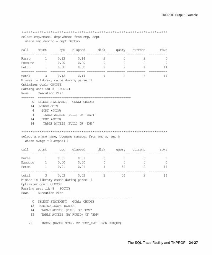
TKPROF Output Example
********************************************************************************select emp.ename, dept.dname from emp, dept where emp.deptno = dept.deptno
call count cpu elapsed disk query current rows------- ------ -------- ---------- ---------- ---------- ---------- ----------Parse 1 0.12 0.14 2 0 2 0Execute 1 0.00 0.00 0 0 0 0Fetch 1 0.00 0.00 2 2 4 14------- ------ -------- ---------- ---------- ---------- ---------- ----------total 3 0.12 0.14 4 2 6 14Misses in library cache during parse: 1Optimizer goal: CHOOSEParsing user id: 8 (SCOTT)Rows Execution Plan------- --------------------------------------------------- 0 SELECT STATEMENT GOAL: CHOOSE 14 MERGE JOIN 4 SORT (JOIN) 4 TABLE ACCESS (FULL) OF ’DEPT’ 14 SORT (JOIN) 14 TABLE ACCESS (FULL) OF ’EMP’
********************************************************************************select a.ename name, b.ename manager from emp a, emp b where a.mgr = b.empno(+)
call count cpu elapsed disk query current rows------- ------ -------- ---------- ---------- ---------- ---------- ----------Parse 1 0.01 0.01 0 0 0 0Execute 1 0.00 0.00 0 0 0 0Fetch 1 0.01 0.01 1 54 2 14------- ------ -------- ---------- ---------- ---------- ---------- ----------total 3 0.02 0.02 1 54 2 14Misses in library cache during parse: 1Optimizer goal: CHOOSEParsing user id: 8 (SCOTT)Rows Execution Plan------- --------------------------------------------------- 0 SELECT STATEMENT GOAL: CHOOSE 13 NESTED LOOPS (OUTER) 14 TABLE ACCESS (FULL) OF ’EMP’ 13 TABLE ACCESS (BY ROWID) OF ’EMP’
26 INDEX (RANGE SCAN) OF ’EMP_IND’ (NON-UNIQUE)
The SQL Trace Facility and TKPROF 24-27
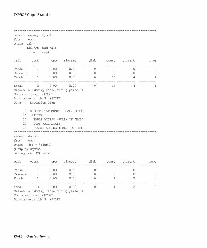
TKPROF Output Example
********************************************************************************select ename,job,salfrom empwhere sal = (select max(sal) from emp)
call count cpu elapsed disk query current rows------- ------ -------- ---------- ---------- ---------- ---------- ----------Parse 1 0.00 0.00 0 0 0 0Execute 1 0.00 0.00 0 0 0 0Fetch 1 0.00 0.00 0 16 4 1------- ------ -------- ---------- ---------- ---------- ---------- ----------total 3 0.00 0.00 0 16 4 1Misses in library cache during parse: 1Optimizer goal: CHOOSEParsing user id: 8 (SCOTT)Rows Execution Plan------- --------------------------------------------------- 0 SELECT STATEMENT GOAL: CHOOSE 14 FILTER 14 TABLE ACCESS (FULL) OF ’EMP’ 14 SORT (AGGREGATE) 14 TABLE ACCESS (FULL) OF ’EMP’********************************************************************************select deptnofrom empwhere job = ’clerk’group by deptnohaving count(*) >= 2
call count cpu elapsed disk query current rows------- ------ -------- ---------- ---------- ---------- ---------- ----------Parse 1 0.00 0.00 0 0 0 0Execute 1 0.00 0.00 0 0 0 0Fetch 1 0.00 0.00 0 1 2 0------- ------ -------- ---------- ---------- ---------- ---------- ----------total 3 0.00 0.00 0 1 2 0Misses in library cache during parse: 1Optimizer goal: CHOOSEParsing user id: 8 (SCOTT)
24-28 Oracle8 Tuning
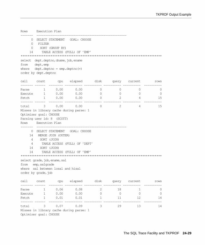
TKPROF Output Example
Rows Execution Plan------- --------------------------------------------------- 0 SELECT STATEMENT GOAL: CHOOSE 0 FILTER 0 SORT (GROUP BY) 14 TABLE ACCESS (FULL) OF ’EMP’********************************************************************************select dept.deptno,dname,job,enamefrom dept,empwhere dept.deptno = emp.deptno(+)order by dept.deptno
call count cpu elapsed disk query current rows------- ------ -------- ---------- ---------- ---------- ---------- ----------Parse 1 0.00 0.00 0 0 0 0Execute 1 0.00 0.00 0 0 0 0Fetch 1 0.00 0.00 0 2 4 15------- ------ -------- ---------- ---------- ---------- ---------- ----------total 3 0.00 0.00 0 2 4 15Misses in library cache during parse: 1Optimizer goal: CHOOSEParsing user id: 8 (SCOTT)Rows Execution Plan------- --------------------------------------------------- 0 SELECT STATEMENT GOAL: CHOOSE 14 MERGE JOIN (OUTER) 4 SORT (JOIN) 4 TABLE ACCESS (FULL) OF ’DEPT’ 14 SORT (JOIN) 14 TABLE ACCESS (FULL) OF ’EMP’********************************************************************************select grade,job,ename,salfrom emp,salgradewhere sal between losal and hisalorder by grade,job
call count cpu elapsed disk query current rows------- ------ -------- ---------- ---------- ---------- ---------- ----------Parse 1 0.06 0.08 2 18 1 0Execute 1 0.00 0.00 0 0 0 0Fetch 1 0.01 0.01 1 11 12 14------- ------ -------- ---------- ---------- ---------- ---------- ----------total 3 0.07 0.09 3 29 13 14Misses in library cache during parse: 1Optimizer goal: CHOOSE
The SQL Trace Facility and TKPROF 24-29
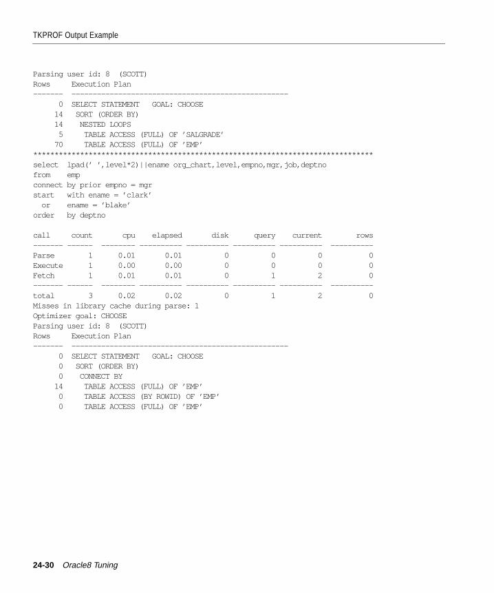
TKPROF Output Example
Parsing user id: 8 (SCOTT)Rows Execution Plan------- --------------------------------------------------- 0 SELECT STATEMENT GOAL: CHOOSE 14 SORT (ORDER BY) 14 NESTED LOOPS 5 TABLE ACCESS (FULL) OF ’SALGRADE’ 70 TABLE ACCESS (FULL) OF ’EMP’********************************************************************************select lpad(’ ’,level*2)||ename org_chart,level,empno,mgr,job,deptnofrom empconnect by prior empno = mgrstart with ename = ’clark’ or ename = ’blake’order by deptno
call count cpu elapsed disk query current rows------- ------ -------- ---------- ---------- ---------- ---------- ----------Parse 1 0.01 0.01 0 0 0 0Execute 1 0.00 0.00 0 0 0 0Fetch 1 0.01 0.01 0 1 2 0------- ------ -------- ---------- ---------- ---------- ---------- ----------total 3 0.02 0.02 0 1 2 0Misses in library cache during parse: 1Optimizer goal: CHOOSEParsing user id: 8 (SCOTT)Rows Execution Plan------- --------------------------------------------------- 0 SELECT STATEMENT GOAL: CHOOSE 0 SORT (ORDER BY) 0 CONNECT BY 14 TABLE ACCESS (FULL) OF ’EMP’ 0 TABLE ACCESS (BY ROWID) OF ’EMP’ 0 TABLE ACCESS (FULL) OF ’EMP’
24-30 Oracle8 Tuning
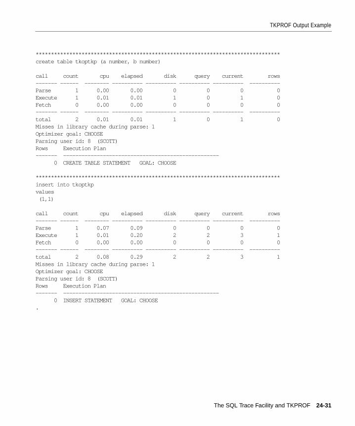
TKPROF Output Example
********************************************************************************create table tkoptkp (a number, b number)
call count cpu elapsed disk query current rows------- ------ -------- ---------- ---------- ---------- ---------- ----------Parse 1 0.00 0.00 0 0 0 0Execute 1 0.01 0.01 1 0 1 0Fetch 0 0.00 0.00 0 0 0 0------- ------ -------- ---------- ---------- ---------- ---------- ----------total 2 0.01 0.01 1 0 1 0Misses in library cache during parse: 1Optimizer goal: CHOOSEParsing user id: 8 (SCOTT)Rows Execution Plan------- --------------------------------------------------- 0 CREATE TABLE STATEMENT GOAL: CHOOSE
********************************************************************************insert into tkoptkpvalues (1,1)
call count cpu elapsed disk query current rows------- ------ -------- ---------- ---------- ---------- ---------- ----------Parse 1 0.07 0.09 0 0 0 0Execute 1 0.01 0.20 2 2 3 1Fetch 0 0.00 0.00 0 0 0 0------- ------ -------- ---------- ---------- ---------- ---------- ----------total 2 0.08 0.29 2 2 3 1Misses in library cache during parse: 1Optimizer goal: CHOOSEParsing user id: 8 (SCOTT)Rows Execution Plan------- --------------------------------------------------- 0 INSERT STATEMENT GOAL: CHOOSE.
The SQL Trace Facility and TKPROF 24-31
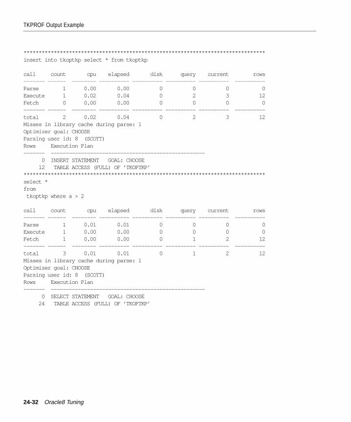
TKPROF Output Example
********************************************************************************insert into tkoptkp select * from tkoptkp
call count cpu elapsed disk query current rows------- ------ -------- ---------- ---------- ---------- ---------- ----------Parse 1 0.00 0.00 0 0 0 0Execute 1 0.02 0.04 0 2 3 12Fetch 0 0.00 0.00 0 0 0 0------- ------ -------- ---------- ---------- ---------- ---------- ----------total 2 0.02 0.04 0 2 3 12Misses in library cache during parse: 1Optimizer goal: CHOOSEParsing user id: 8 (SCOTT)Rows Execution Plan------- --------------------------------------------------- 0 INSERT STATEMENT GOAL: CHOOSE 12 TABLE ACCESS (FULL) OF ’TKOPTKP’********************************************************************************select *from tkoptkp where a > 2
call count cpu elapsed disk query current rows------- ------ -------- ---------- ---------- ---------- ---------- ----------Parse 1 0.01 0.01 0 0 0 0Execute 1 0.00 0.00 0 0 0 0Fetch 1 0.00 0.00 0 1 2 12------- ------ -------- ---------- ---------- ---------- ---------- ----------total 3 0.01 0.01 0 1 2 12Misses in library cache during parse: 1Optimizer goal: CHOOSEParsing user id: 8 (SCOTT)Rows Execution Plan------- --------------------------------------------------- 0 SELECT STATEMENT GOAL: CHOOSE 24 TABLE ACCESS (FULL) OF ’TKOPTKP’
24-32 Oracle8 Tuning
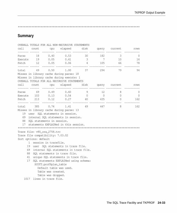
TKPROF Output Example
********************************************************************************
Summary
OVERALL TOTALS FOR ALL NON-RECURSIVE STATEMENTScall count cpu elapsed disk query current rows------- ------ -------- ---------- ---------- ---------- ---------- ----------Parse 18 0.40 0.53 30 182 3 0Execute 19 0.05 0.41 3 7 10 16Fetch 12 0.05 0.06 4 105 66 78------- ------ -------- ---------- ---------- ---------- ---------- ----------total 49 0.50 1.00 37 294 79 94Misses in library cache during parse: 18Misses in library cache during execute: 1OVERALL TOTALS FOR ALL RECURSIVE STATEMENTScall count cpu elapsed disk query current rows------- ------ -------- ---------- ---------- ---------- ---------- ----------Parse 69 0.49 0.60 9 12 8 0Execute 103 0.13 0.54 0 0 0 0Fetch 213 0.12 0.27 40 435 0 162------- ------ -------- ---------- ---------- ---------- ---------- ----------total 385 0.74 1.41 49 447 8 162Misses in library cache during parse: 13 19 user SQL statements in session. 69 internal SQL statements in session. 88 SQL statements in session. 17 statements EXPLAINed in this session.********************************************************************************Trace file: v80_ora_2758.trcTrace file compatibility: 7.03.02Sort options: default 1 session in tracefile. 19 user SQL statements in trace file. 69 internal SQL statements in trace file. 88 SQL statements in trace file. 41 unique SQL statements in trace file. 17 SQL statements EXPLAINed using schema: SCOTT.prof$plan_table Default table was used. Table was created. Table was dropped. 1017 lines in trace file.
The SQL Trace Facility and TKPROF 24-33

TKPROF Output Example
24-34 Oracle8 Tuning
Using Oracl
25
Using Oracle TraceThis chapter describes how to use Oracle Trace to collect Oracle Server event data.It covers:
■ Introduction
■ Using Oracle Trace for Server Performance Data Collection
■ Using Initialization Parameters to Control Oracle Trace
■ Using Stored Procedure Packages to Control Oracle Trace
■ Using the Oracle Trace Command-Line Interface
■ Oracle Trace Collection Results
e Trace 25-1
Introduction
IntroductionOracle Trace is a general-purpose data collection product that has been introducedwith the Oracle Enterprise Manager systems management product family. You canuse the Oracle Trace data collection API in any software product to collect data fora variety of uses, such as performance monitoring, diagnostics, and auditing. Ora-cle Trace collects specific data for events defined within the host product.
The server performance data that you can collect with Oracle Trace includes:
■ SQL statements and statistics on the frequency, duration, and resources usedfor all parse, execution, and fetch events
■ Execution plan details
■ Logical and physical database transactions, including the frequency, duration,and resources used by each transaction event
■ A set of statistics associated with each of these duration events, including:UGA and PGA memory, block changes, block gets, consistent gets, physicalreads, redo entries, redo size, sorts in memory and disk
■ Resource usage for each database event measured in CPU time, file I/Os andpage faults
See Also: Oracle Trace User’s Guide and Oracle Trace Developer’s Guide contained inthe Oracle Enterprise Manager Performance Pack documentation set. These bookscontain a complete list of events and data that can be collected for Oracle Server.
25-2 Oracle8 Tuning
Using Oracle Trace for Server Performance Data Collection
Using Oracle Trace for Server Performance Data CollectionYou can use Oracle Trace to collect server performance data for a specific databasesession or for the entire instance. You can also select the server event set for whichyou want to collect.
Oracle Trace lets you organize host application events into event sets. Doing soallows you to collect data for a specific subset of all potential host applicationevents. Oracle has defined the following event sets: ALL, DEFAULT, and EXPERT.The ALL set includes all server events, the DEFAULT set excludes server WAITevents, and the EXPERT set is specifically defined for use in the Oracle Expert tun-ing application. Oracle recommends using the DEFAULT event set.
You can enable and control server collections in the following ways:
■ Using the Oracle Trace Manager application, a Windows-based graphical userinterface that is supplied with the Oracle Enterprise Manager PerformancePack (a database option you can license)
■ Using nongraphical, server-based controls:
– Oracle Trace database initialization parameters
– Oracle Trace stored procedure packages
– Oracle Trace Command-Line Interface
The following sections describe the server-based controls.
See Also: Oracle Trace User’s Guide
Using Oracle Trace 25-3
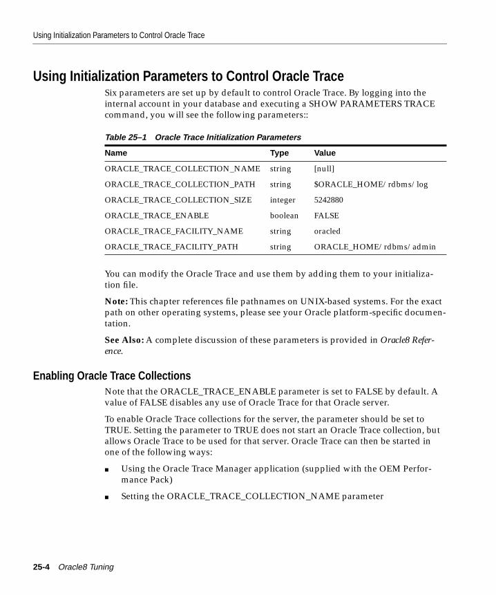
Using Initialization Parameters to Control Oracle Trace
Using Initialization Parameters to Control Oracle TraceSix parameters are set up by default to control Oracle Trace. By logging into theinternal account in your database and executing a SHOW PARAMETERS TRACEcommand, you will see the following parameters::
You can modify the Oracle Trace and use them by adding them to your initializa-tion file.
Note: This chapter references file pathnames on UNIX-based systems. For the exactpath on other operating systems, please see your Oracle platform-specific documen-tation.
See Also: A complete discussion of these parameters is provided in Oracle8 Refer-ence.
Enabling Oracle Trace CollectionsNote that the ORACLE_TRACE_ENABLE parameter is set to FALSE by default. Avalue of FALSE disables any use of Oracle Trace for that Oracle server.
To enable Oracle Trace collections for the server, the parameter should be set toTRUE. Setting the parameter to TRUE does not start an Oracle Trace collection, butallows Oracle Trace to be used for that server. Oracle Trace can then be started inone of the following ways:
■ Using the Oracle Trace Manager application (supplied with the OEM Perfor-mance Pack)
■ Setting the ORACLE_TRACE_COLLECTION_NAME parameter
Table 25–1 Oracle Trace Initialization Parameters
Name Type Value
ORACLE_TRACE_COLLECTION_NAME string [null]
ORACLE_TRACE_COLLECTION_PATH string $ORACLE_HOME/rdbms/log
ORACLE_TRACE_COLLECTION_SIZE integer 5242880
ORACLE_TRACE_ENABLE boolean FALSE
ORACLE_TRACE_FACILITY_NAME string oracled
ORACLE_TRACE_FACILITY_PATH string ORACLE_HOME/rdbms/admin
25-4 Oracle8 Tuning
Using Initialization Parameters to Control Oracle Trace
When ORACLE_TRACE_ENABLE is set to TRUE, you can initiate an Oracle Traceserver collection by entering a collection name in theORACLE_TRACE_COLLECTION_NAME parameter. The default value for thisparameter is NULL. A collection name can be up to 16 characters long. You mustthen shut down your database and start it up again before the parameters takeeffect. If a collection name is specified, when you start the server, you automaticallystart an Oracle Trace collection for all database sessions.
To stop the collection, shut down the server instance and reset theORACLE_TRACE_COLLECTION_NAME to NULL. The collection name specifiedin this value is also used in two collection output file names: the collection defini-tion file (collection_name.cdf) and the binary data file (collection_name.dat).
Determining the Event Set Which Oracle Trace Collects The ORACLE_TRACE_FACILITY_NAME determines the event set that OracleTrace will collect. The name of the DEFAULT event set is ORACLED. The ALLevent set is ORACLE and the EXPERT event set is ORACLEE.
If, once restarted, the database does not start collecting data, you should check thefollowing:
■ The event set file, identified by the ORACLE_TRACE_FACILITY_NAME (with.fdf appended to it) should be located in the directory identified byORACLE_TRACE_FACILITY_PATH.
■ The following files should exist in your Oracle Trace admin directory:REGID.DAT, PROCESS.DAT, and COLLECT.DAT. If they do not, you must runthe OTRCCREF executable to create them.
■ The Oracle Trace parameters should be set to the values that you changed inthe initialization file.
■ Look for an EPC_ERROR.LOG file. It will give you more information aboutwhy a collection may have failed.
Using Oracle Trace 25-5
Using Stored Procedure Packages to Control Oracle Trace
Using Stored Procedure Packages to Control Oracle TraceUsing the Oracle Trace stored procedure packages you can invoke an Oracle Tracecollection for your own session or for another session. To collect Oracle Trace datafor your own database session, execute the following stored procedure package:
DBMS_ORACLE_TRACE_USER.SET_ORACLE_TRACE(TRUE/FALSE, collection_name,server_event_set)
■ true/false = Boolean: TRUE to turn on, FALSE to turn off
■ collection_name = varchar2: collection name (no file extension, 8 character max-imum)
■ server_event_set = varchar2: server event set (oracled, oracle, or oraclee)
Example:
EXECUTE DBMS_ORACLE_TRACE_USER.SET_ORACLE_TRACE (TRUE,"MYCOLL","oracle");
To collect Oracle Trace data for a database session other than your own, execute thefollowing stored procedure package:
DBMS_ORACLE_TRACE_AGENT.SET_ORACLE_TRACE_IN_SESSION(sid, serial#, true/false,collection_name, server_event_set)
■ sid = number: session instance from v$session.sid
■ serial# = number: session serial number from v$session.serial#
Example:
EXECUTE DBMS_ORACLE_TRACE_USER.SET_ORACLE_TRACE_IN_SESSION (8,12,TRUE,"MYCOLL","oracled");
If the collection does not occur, you should check the following:
■ Be sure the server event set file identified by server_event_set exists. If there isno full file specification on this field, then the file should be located in the direc-tory identified by ORACLE_TRACE_FACILITY_PATH in the initialization file.
■ The following files should exist in your Oracle Trace admin directory:REGID.DAT, PROCESS.DAT, and COLLECT.DAT. If they do not, you must runthe otrccref executable to create them.
■ The stored procedure packages should exist in the database. If the packages donot exist, you must run the OTRCSVR.SQL file (in your Oracle Trace admindirectory) to create the packages.
25-6 Oracle8 Tuning
Using the Oracle Trace Command-Line Interface
Using the Oracle Trace Command-Line InterfaceAnother option for controlling Oracle Trace server collections is the Oracle Tracecommand-line interface (CLI). The CLI collects event data for all server sessionsattached to the database at collection start time. Sessions that attach after the collec-tion is started are excluded from the collection. The CLI is invoked by the otrccolcommand for the following functions:
■ OTRCCOL START job_id input_parameter_file
■ OTRCCOL STOP job_id input_parameter_file
■ OTRCCOL FORMAT input_parameter_file
■ OTRCCOL DCF coll_name cdf_file
■ OTRCCOL DFD coll_name username password service
The parameter JOB_ID can be any numeric value. (You must remember this valuein order to stop the collection.) The input parameter file contains specific parametervalues required for each function. Examples follow. COLL_NAME (collectionname) and CDF_FLE (collection definition file) are initially defined in the STARTfunction input parameter file.
The OTRCCOL START command invokes a collection based upon parameter val-ues contained in the input parameter file. For example:
otrccol start 1234 my_start_input_file
where my_start_input_file contains the following input parameters:
col_name= my_collectiondat_file= <usually same as collection name>.datcdf_file= <usually same as collection name>.cdffdf_file= <server event set>.fdfregid= 1 192216243 0 0 5 <database SID>
The server event sets that can be used as values for the fdf_file are ORACLE, ORA-CLED, and ORACLEE. See "Using Initialization Parameters to Control OracleTrace" on page 25-4 for more information on the server event sets.
The OTRCCOL STOP command halts a running collection, as follows:
otrccol stop 1234 my_stop_input_file
where my_stop_input_file contains the collection name and cdf_file name.
Using Oracle Trace 25-7
Oracle Trace Collection Results
The OTRCCOL FORMAT command formats the binary collection file to Oracletables. An example of the FORMAT command is as follows:
otrccol format my_format_input_file
where my_format_input_file contains the following input parameters
username= <database username>password= <database password>service= <database service name>cdf_file= <usually same as collection name>.cdffull_format= <0/1>
A full_format value of 1 produces a full format; a value of 0 produces a partial for-mat. See "Formatting Oracle Trace Data to Oracle Tables" on page 25-10 for informa-tion on formatting part or all of an Oracle Trace collection, and other importantinformation on creating the Oracle Trace formatting tables prior to running the for-mat command.
The OTRCCOL DCF command deletes collection files for a specific collection. TheOTRCCOL DFD command deletes formatted data from the Oracle Trace formattertables for a specific collection.
Oracle Trace Collection ResultsRunning an Oracle Trace collection produces the following collection files:
■ collection_name.CDF is the Oracle Trace collection definition file for your col-lection.
■ collection_name.DAT files are the Oracle Trace output files containing the tracedata in binary format.
You can access the Oracle Trace data in the collection files in two ways:
■ You can create Oracle Trace Detail Reports from the binary file.
■ The data can be formatted to Oracle tables for SQL access and reporting.
25-8 Oracle8 Tuning
Oracle Trace Collection Results
Oracle Trace Detail ReportsOracle Trace Detail Reports display statistics for all items associated with eachoccurrence of a server event. These reports can be quite large. You can control thereport output by using command parameters. Use the following command andoptional parameters to produce a Detail Report:
OTRCREP [optional parameters] collection_name.CDF
The first step that you may want to take is to run a report called PROCESS.txt. Youcan produce this report first to give you a listing of specific process identifiers forwhich you want to run the detail report.
The command parameter used to produce a Process report is:
OTRCREP -P collection_name.CDF
Other optional detail report parameters are:
output_path specifies a full output path for the report files. If notspecified, the files will be placed in the current directory
-p creates a report for a specific process ID obtained from thePROCESS report. For example, a detail report for process1234 would use -p1234
-w# sets report width, such as -w132. The default is 80characters.
-l# sets the number of report lines per page. The default is 63lines per page.
-h suppresses all event and item report headers, producing ashorter report
-s used with Net8 data only
-a creates a report containing all the events for all products, inthe order they occur in the data collection (.dat) file. Thereport is a text display of all items for all events.
Using Oracle Trace 25-9
Oracle Trace Collection Results
Formatting Oracle Trace Data to Oracle TablesYour Oracle Trace server collection can be formatted to Oracle tables for more flexi-ble access by any SQL reporting tool. Oracle Trace will produce a separate table foreach event collected. For example, a “parses” event table is created to store data forall parse events that occur during a server collection. Before you can format data,you must first set up the Oracle Trace formatter tables by executing theOTRCFMTC.SQL script on the server host machine.
Use the following command to format an Oracle Trace collection:
OTRCFMT [optional parameters] collection_name.cdf [user/password@database]
If user/password@database is omitted, the user will be prompted for this informa-tion.
Oracle Trace allows data to be formatted while a collection is occurring. By default,Oracle Trace formats only the portion of the collection that has not been formattedpreviously. If you want to reformat the entire collection file, use the optional param-eter -f.
Oracle Trace provides several SQL scripts that you can use to access the serverevent tables. For more information on server event tables and scripts for accessingevent data and improving event table performance, refer to the Oracle Trace User’sGuide
25-10 Oracle8 Tuning
Registering Appli
26
Registering ApplicationsApplication developers can use the DBMS_APPLICATION_INFO package withOracle Trace and the SQL trace facility to record the name of the executing moduleor transaction in the database for use later when tracking the performance of vari-ous modules. This chapter describes how to register an application with the data-base and retrieve statistics on each registered module or code segment. Topics inthis chapter include:
■ Overview
■ Registering Applications
■ Setting the Module Name
■ Setting the Action Name
■ Setting the Client Information
■ Retrieving Application Information
cations 26-1
Overview
OverviewOracle provides a method for applications to register the name of the applicationand actions performed by that application with the database. Registering the appli-cation allows system administrators and performance tuning specialists to trackperformance by module. System administrators can also use this information totrack resource use by module. When an application registers with the database, itsname and actions are recorded in the V$SESSION and V$SQLAREA views.
Your applications should set the name of the module and name of the action auto-matically each time a user enters that module. The module name could be the nameof a form in an Oracle Forms application, or the name of the code segment in anOracle Precompilers application. The action name should usually be the name ordescription of the current transaction within a module.
Registering ApplicationsTo register applications with the database, use the procedures in theDBMS_APPLICATION_INFO package.
DBMS_APPLICATION_INFO PackageDBMS_APPLICATION_INFO provides the following procedures:
PrivilegesBefore using this package, you must run the DBMSUTL.SQL script to create theDBMS_APPLICATION_INFO package. For more information about Oracle sup-plied packages and executing stored procedures, see the Oracle8 Application Devel-oper’s Guide.
Table 26–1 Procedures in the DBMS_APPLICATION_INFO Package
Procedure Description
SET_MODULE Sets the name of the module that is currently running.
SET_ACTION Sets the name of the current action within the current module.
SET_CLIENT_INFO Sets the client information field for the session.
READ_MODULE Reads values of module and action fields for the current session.
READ_CLIENT_INFO Reads the client information field for the current session.
26-2 Oracle8 Tuning
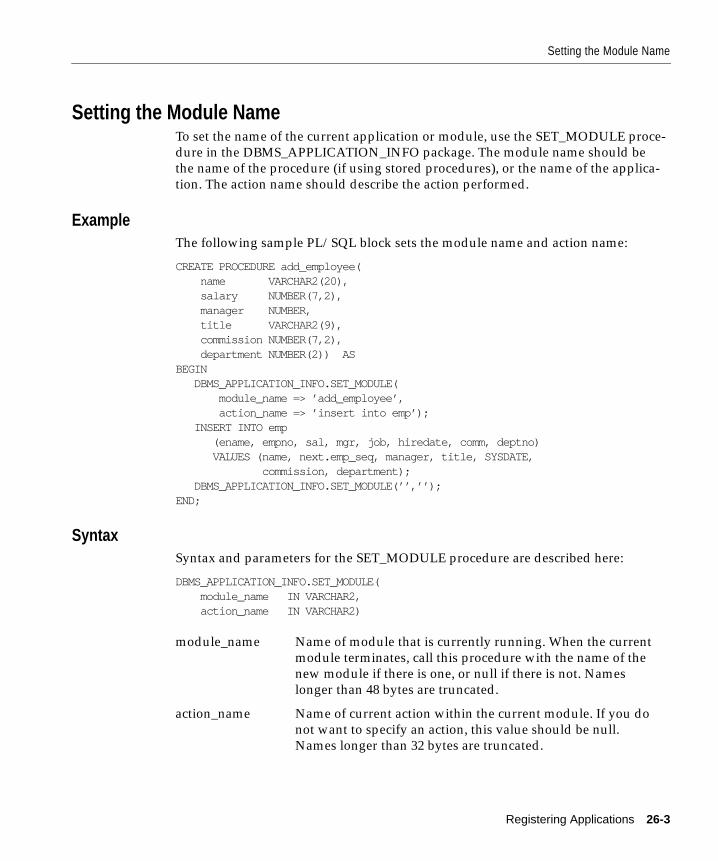
Setting the Module Name
Setting the Module NameTo set the name of the current application or module, use the SET_MODULE proce-dure in the DBMS_APPLICATION_INFO package. The module name should bethe name of the procedure (if using stored procedures), or the name of the applica-tion. The action name should describe the action performed.
ExampleThe following sample PL/SQL block sets the module name and action name:
CREATE PROCEDURE add_employee( name VARCHAR2(20), salary NUMBER(7,2), manager NUMBER, title VARCHAR2(9), commission NUMBER(7,2), department NUMBER(2)) ASBEGIN DBMS_APPLICATION_INFO.SET_MODULE( module_name => ’add_employee’, action_name => ’insert into emp’); INSERT INTO emp (ename, empno, sal, mgr, job, hiredate, comm, deptno) VALUES (name, next.emp_seq, manager, title, SYSDATE, commission, department); DBMS_APPLICATION_INFO.SET_MODULE(’’,’’);END;
SyntaxSyntax and parameters for the SET_MODULE procedure are described here:
DBMS_APPLICATION_INFO.SET_MODULE( module_name IN VARCHAR2, action_name IN VARCHAR2)
module_name Name of module that is currently running. When the currentmodule terminates, call this procedure with the name of thenew module if there is one, or null if there is not. Nameslonger than 48 bytes are truncated.
action_name Name of current action within the current module. If you donot want to specify an action, this value should be null.Names longer than 32 bytes are truncated.
Registering Applications 26-3
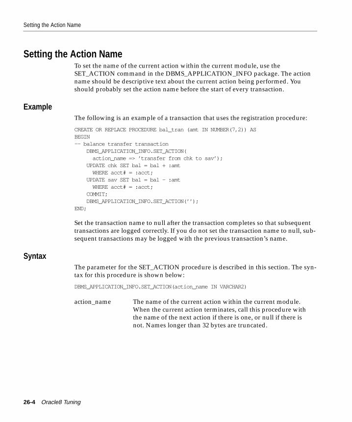
Setting the Action Name
Setting the Action NameTo set the name of the current action within the current module, use theSET_ACTION command in the DBMS_APPLICATION_INFO package. The actionname should be descriptive text about the current action being performed. Youshould probably set the action name before the start of every transaction.
ExampleThe following is an example of a transaction that uses the registration procedure:
CREATE OR REPLACE PROCEDURE bal_tran (amt IN NUMBER(7,2)) ASBEGIN-- balance transfer transaction DBMS_APPLICATION_INFO.SET_ACTION( action_name => ’transfer from chk to sav’); UPDATE chk SET bal = bal + :amt WHERE acct# = :acct; UPDATE sav SET bal = bal - :amt WHERE acct# = :acct; COMMIT; DBMS_APPLICATION_INFO.SET_ACTION(’’);END;
Set the transaction name to null after the transaction completes so that subsequenttransactions are logged correctly. If you do not set the transaction name to null, sub-sequent transactions may be logged with the previous transaction’s name.
SyntaxThe parameter for the SET_ACTION procedure is described in this section. The syn-tax for this procedure is shown below:
DBMS_APPLICATION_INFO.SET_ACTION(action_name IN VARCHAR2)
action_name The name of the current action within the current module.When the current action terminates, call this procedure withthe name of the next action if there is one, or null if there isnot. Names longer than 32 bytes are truncated.
26-4 Oracle8 Tuning
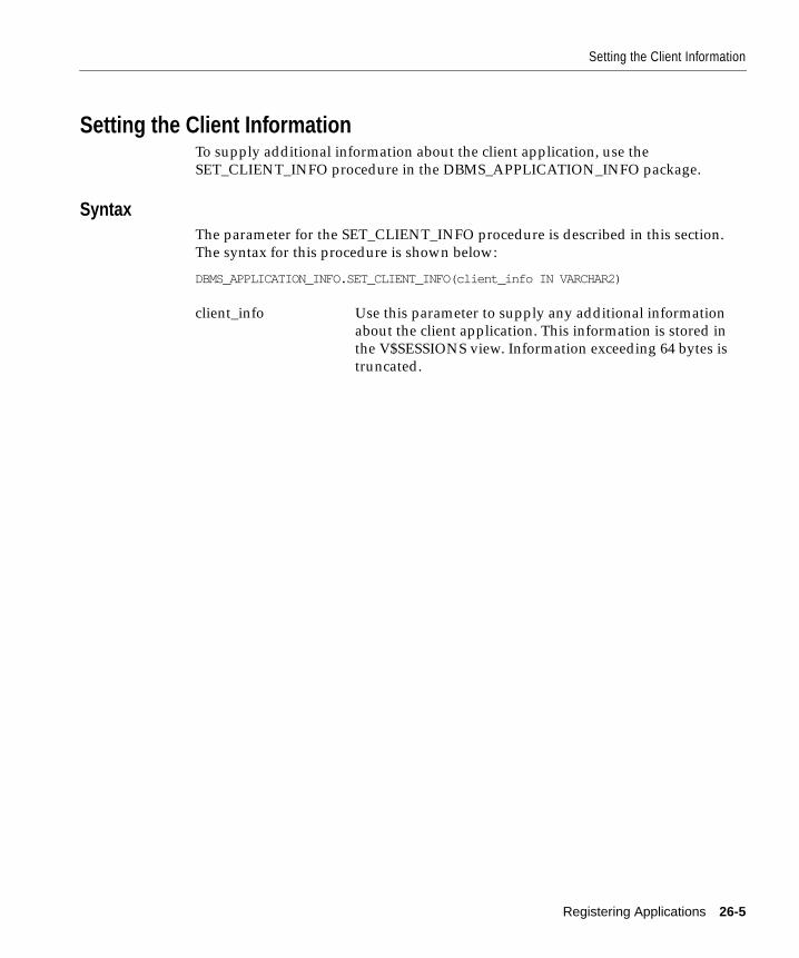
Setting the Client Information
Setting the Client InformationTo supply additional information about the client application, use theSET_CLIENT_INFO procedure in the DBMS_APPLICATION_INFO package.
SyntaxThe parameter for the SET_CLIENT_INFO procedure is described in this section.The syntax for this procedure is shown below:
DBMS_APPLICATION_INFO.SET_CLIENT_INFO(client_info IN VARCHAR2)
client_info Use this parameter to supply any additional informationabout the client application. This information is stored inthe V$SESSIONS view. Information exceeding 64 bytes istruncated.
Registering Applications 26-5
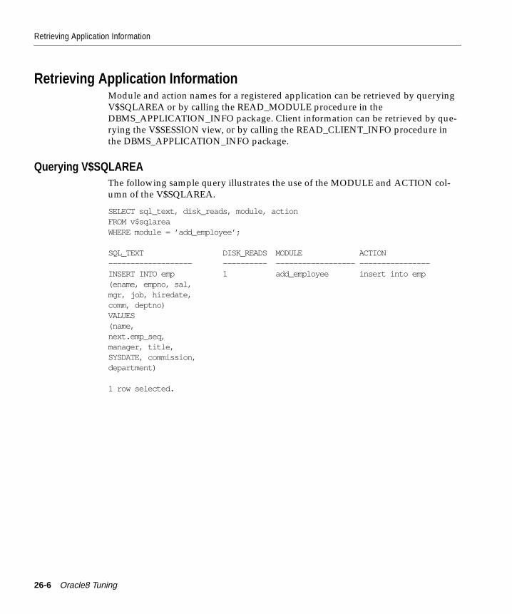
Retrieving Application Information
Retrieving Application InformationModule and action names for a registered application can be retrieved by queryingV$SQLAREA or by calling the READ_MODULE procedure in theDBMS_APPLICATION_INFO package. Client information can be retrieved by que-rying the V$SESSION view, or by calling the READ_CLIENT_INFO procedure inthe DBMS_APPLICATION_INFO package.
Querying V$SQLAREAThe following sample query illustrates the use of the MODULE and ACTION col-umn of the V$SQLAREA.
SELECT sql_text, disk_reads, module, actionFROM v$sqlareaWHERE module = ’add_employee’;
SQL_TEXT DISK_READS MODULE ACTION------------------- ---------- ------------------ ----------------INSERT INTO emp 1 add_employee insert into emp(ename, empno, sal,mgr, job, hiredate,comm, deptno)VALUES(name,next.emp_seq,manager, title,SYSDATE, commission,department)
1 row selected.
26-6 Oracle8 Tuning
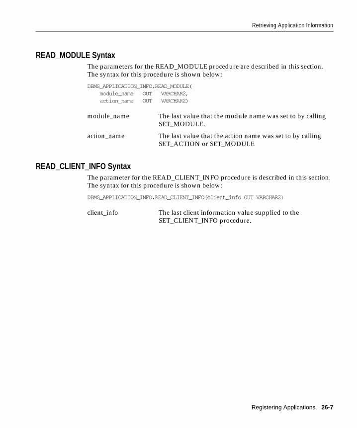
Retrieving Application Information
READ_MODULE SyntaxThe parameters for the READ_MODULE procedure are described in this section.The syntax for this procedure is shown below:
DBMS_APPLICATION_INFO.READ_MODULE( module_name OUT VARCHAR2, action_name OUT VARCHAR2)
READ_CLIENT_INFO SyntaxThe parameter for the READ_CLIENT_INFO procedure is described in this section.The syntax for this procedure is shown below:
DBMS_APPLICATION_INFO.READ_CLIENT_INFO(client_info OUT VARCHAR2)
module_name The last value that the module name was set to by callingSET_MODULE.
action_name The last value that the action name was set to by callingSET_ACTION or SET_MODULE
client_info The last client information value supplied to theSET_CLIENT_INFO procedure.
Registering Applications 26-7

Retrieving Application Information
26-8 Oracle8 Tuning
Index
AABORTED_REQUEST_THRESHOLDprocedure, 14-23access path, 2-10aggregate, 20-3, 20-18alert log, 4-3ALL_HISTOGRAMS, 8-4ALL_INDEXES view, 10-16ALL_OBJECTS view, 14-38ALL_ROWS hint, 8-14ALL_TAB_COLUMNS, 8-4allocation, of memory, 14-2ALTER INDEX REBUILD statement, 10-10ALTER SESSION command
examples, 24-5SET SESSION_CACHED_CURSORS, 14-18
ALTER SYSTEM commandMTS_DISPATCHERS parameter, 18-8
ALTER TABLE commandNOLOGGING option, 20-26
ALWAYS_ANTI_JOIN parameter, 8-8, 19-16, 19-17ALWAYS_SEMI_JOIN parameter, 19-17analysis dictionary, 4-4ANALYZE command, 6-4, 15-32, 19-45, 20-20,
20-24COMPUTE option, 19-45ESTIMATE option, 19-45examples, 8-5
ANALYZE INDEX statement, 19-46analyzing data, 19-45AND_EQUAL hint, 8-23, 10-8anti-join, 19-16APPEND hint, 8-29, 20-26
application design, 2-9application designer, 1-8application developer, 1-8applications
client/server, 5-9decision support, 5-4, 19-2distributed databases, 5-7OLTP, 5-2parallel query, 5-5parallel server, 5-9registering with the database, 4-7, 26-2
ARCH process, 18-13ARCH process, multiple, 19-43architecture and CPU, 13-10array interface, 16-3asynchronous I/O, 19-21asynchronous operation, 19-21asynchronous readahead, 19-32audit trail, 4-4
BB*-tree index, 10-15, 10-19backup
data warehouse, 6-8disk mirroring, 19-30
BACKUP_DISK_IO_SLAVES parameter, 19-21BACKUP_TAPE_IO_SLAVES parameter, 19-21bandwidth, 19-2BEGIN_DISCRETE_TRANSACTION
procedure, 11-2, 11-4benefit of tuning, 2-3bind variables, 14-16BITMAP CONVERSION row source, 10-19
Index-1
bitmap index, 6-7, 10-13, 10-18creating, 10-16inlist iterator, 23-12maintenance, 10-15size, 10-20storage considerations, 10-14when to use, 10-13
BITMAP keyword, 10-16BITMAP_MERGE_AREA_SIZE parameter, 8-8,
10-15, 10-18block contention, 2-12block size, 15-15bottlenecks
disk I/O, 15-21memory, 14-2
buffer cache, 2-11adding buffers, 14-32memory allocation, 14-29partitioning, 14-39performance statistics, 14-29reducing buffers, 14-32reducing cache misses, 14-29tuning, 14-26
buffer get, 7-5buffer pool
default cache, 14-37keep cache, 14-37multiple, 14-37, 14-38recycle cache, 14-37syntax, 14-40
BUFFER_POOL clause, 14-40BUFFER_POOL_name parameter, 14-39business rule, 1-8, 2-3, 2-7
CCACHE hint, 8-32cardinality, 10-20CATPARR.SQL script, 14-29CATPERF.SQL file, 14-42chained rows, 15-32channel bandwidth, 3-6checkpoints
choosing checkpoint frequency, 15-42current write batch size, 15-44
performance, 15-41redo log maintenance, 15-42tuning, 15-41
CHOOSE hint, 8-16CKPT process, 15-43client/server applications, 5-9, 13-5CLUSTER hint, 8-18clusters, 10-24columns, to index, 10-5COMPATIBLE parameter, 10-16, 19-36
and parallel query, 19-18COMPLEX_VIEW_MERGING parameter, 8-7, 8-9,
8-33composite indexes, 10-6COMPUTE option, 19-45CONNECT BY, 23-14Connection Manager, 16-4connection pooling, 18-9consistency, read, 13-8consistent gets statistic, 14-26, 14-30, 14-34, 18-5,
18-18consistent mode, TKPROF, 24-14constraint, 10-11contention
disk access, 15-21free lists, 18-17memory, 14-2memory access, 18-1redo allocation latch, 18-16redo copy latches, 18-16rollback segments, 18-4tuning, 18-1tuning resource, 2-12
context area, 2-11context switching, 13-5cost-based optimization, 6-7, 8-2, 20-24
parallel query, 20-24COUNT column, 14-29, 14-33count column, SQL trace, 24-14CPU
checking utilization, 13-4detecting problems, 13-4insufficient, 3-5system architecture, 13-10tuning, 13-1
Index-2
utilization, 13-2, 19-2CPU bound operations, 19-32cpu column, SQL trace, 24-14CREATE CLUSTER command, 10-26CREATE INDEX command, 20-21
examples, 15-39NOSORT option, 15-39
CREATE TABLE AS SELECT, 6-3, 20-19, 21-5CREATE TABLE command
STORAGE clause, 15-24TABLESPACE clause, 15-24
CREATE TABLESPACE command, 15-24CREATE TABLESPACE statement, 15-24CREATE_BITMAP_AREA_SIZE parameter, 10-15,
10-18current column, SQL trace, 24-14current mode, TKPROF, 24-14CURSOR_NUM column
TKPROF_TABLE, 24-20CURSOR_SPACE_FOR_TIME parameter
setting, 14-17
Ddata
comparative, 4-5sources for tuning, 4-2volume, 4-2
data block size, 15-15data cache, 17-2data design
tuning, 2-8data dictionary, 4-3data dictionary cache, 2-11, 14-20data warehouse
ANALYZE command, 6-4backup, 6-8bitmap index, 6-7features, 6-1introduction, 6-2Oracle Parallel Server, 6-5parallel aware optimizer, 6-6parallel index creation, 6-3parallel load, 6-4partition, 6-4
partitioned table, 19-31recovery, 6-8star schema, 6-7
database administrator (DBA), 1-8database buffers, 14-32database layout, 19-22database writer process (DBWn)
behavior on checkpoints, 15-41tuning, 13-8, 19-44
DATAFILE clause, 15-24datafile placement on disk, 15-21DATE_OF_INSERT column
TKPROF_TABLE, 24-20DB BLOCK GETS, 14-34db block gets statistic, 14-26, 14-30, 18-5, 18-18DB_BLOCK_BUFFERS parameter, 14-29, 14-32,
14-40, 15-44DB_BLOCK_CHECKPOINT_BATCH
parameter, 15-44DB_BLOCK_LRU_EXTENDED_STATISTICS
parameter, 14-30DB_BLOCK_LRU_LATCHES parameter, 14-40,
14-45DB_BLOCK_LRU_STATISTICS parameter, 14-33DB_BLOCK_SIZE parameter
and parallel query, 19-19DB_FILE_MULTIBLOCK_READ_COUNT
parameter, 8-7, 15-38, 19-19DBA locking, 20-13DBA_DATA_FILES view, 21-10DBA_EXTENTS view, 21-10DBA_HISTOGRAMS, 8-4DBA_INDEXES view, 10-16DBA_OBJECTS view, 14-38DBA_TAB_COLUMNS, 8-4DBMS_APPLICATION_INFO package, 26-2, 26-4DBMS_SHARED_POOL package, 12-4, 14-12,
14-23DBMS_SYSTEM package, 24-6DBMS_SYSTEM.SET_SQL_TRACE_IN_SESSION
procedure, 24-6DBMS_UTILITY.ANALYZE_PART_OBJECT,
19-45DBMSPOOL.SQL script, 12-4, 14-12DBMSUTL.SQL, 26-2
Index-3
DBWR_IO_SLAVES parameter, 19-21decision support, 5-4
processes, 20-3query characteristics, 19-4systems (DSS), 1-2tuning, 19-2with OLTP, 5-6
decomposition of SQL statements, 9-4default cache, 14-37demand rate, 1-5, 1-6DEPTH column
TKPROF_TABLE, 24-20design dictionary, 4-4designing and tuning, 2-10device bandwidth, 3-6
evaluating, 15-16device latency, 3-6diagnosing tuning problems, 3-1dimension table, 6-7direct-load insert, 19-44, 20-29
external fragmentation, 20-13disabled constraint, 10-11discrete transactions
example, 11-4processing, 11-3, 11-4when to use, 11-2
disk affinityand parallel query, 20-15disabling with MPP, 19-26with MPP, 19-41
disk column, SQL trace, 24-14DISK_ASYNCH_IO parameter, 19-21disks
contention, 15-21distributing I/O, 15-21I/O requirements, 15-4layout options, 15-15monitoring OS file activity, 15-17number required, 15-4placement of datafiles, 15-21placement of redo log files, 15-21reducing contention, 15-21speed characteristics, 15-4testing performance, 15-6
dispatcher processes (Dnnn), 18-8
distributed databases, 5-7distributed query, 9-1, 9-12distributing I/O, 15-21, 15-24DIUTIL package, 12-5DML_LOCKS parameter, 19-14, 19-15DSS memory, 19-3dynamic extension, 15-27dynamic performance views
enabling statistics, 24-4for tuning, 22-1parallel operations, 21-10
Eelapsed column, SQL trace, 24-14enabled constraint, 10-11enforced constraint, 10-11ENQUEUE_RESOURCES parameter, 19-14, 19-15Enterprise Manager, 4-7equijoin, 7-9errors
common tuning, 2-15during discrete transactions, 11-3
ESTIMATE option, 19-45examples
ALTER SESSION command, 24-5ANALYZE command, 8-5CREATE INDEX command, 15-39CREATE TABLE command, 15-24CREATE TABLESPACE command, 15-24DATAFILE clause, 15-24discrete transactions, 11-4execution plan, 7-7EXPLAIN PLAN output, 7-7, 23-13, 24-17full table scan, 7-8indexed query, 7-8NOSORT option, 15-39SET TRANSACTION command, 15-30SQL trace facility output, 24-17STORAGE clause, 15-24table striping, 15-24TABLESPACE clause, 15-24
executable code as data source, 4-4execution plans, 23-2
examples, 7-7, 24-8
Index-4
parallel operations, 21-5TKPROF, 24-8, 24-10
EXISTS subquery, 19-17expectations for tuning, 1-9Expert, Oracle, 4-12EXPLAIN PLAN command
examples of output, 7-7, 23-13, 24-17introduction, 4-6invoking with the TKPROF program, 24-10parallel query, 21-4PLAN_TABLE, 23-3query parallelization, 21-8SQL decomposition, 9-7
extentssize, 19-35temporary, 19-40unlimited, 15-29
Ffact table, 6-7failover, 6-5FAST FULL SCAN, 6-3, 10-9FAST_FULL_SCAN_ENABLED parameter, 10-9file storage, designing, 15-5FIRST_ROWS hint, 8-15, 19-5fragmentation, external, 20-13free lists
adding, 18-18contention, 18-17reducing contention, 18-18
FREELISTS, 19-43FULL hint, 8-17, 10-8full table scan, 7-8
GGC_FILES_TO_LOCKS parameter, 20-13GC_ROLLBACK_LOCKS parameter, 20-14GC_ROLLBACK_SEGMENTS parameter, 20-14GETMISSES, V$ROWCACHE table, 14-20GETS, V$ROWCACHE table, 14-20global dynamic performance view, 21-10global index, 19-42goals for tuning, 1-9, 2-13
GROUP BYdecreasing demand for, 20-7example, 21-9NOSORT, 15-39
GV$ views, querying, 19-7GV$CURRENT_BUCKET view, 14-29GV$FILESTAT view, 21-10GV$RECENT_BUCKET view, 14-29
Hhash area, 2-11, 20-3HASH hint, 8-18hash join, 19-4, 20-3HASH parameter
CREATE CLUSTER command, 10-26HASH_AJ hint, 8-19, 19-16, 19-17HASH_AREA_SIZE parameter
and parallel execution, 19-4example, 20-7relationship to memory, 20-6
HASH_JOIN_ENABLED parameter, 8-8HASH_MULTIBLOCK_IO_COUNT parameter,
8-8, 19-19HASH_SJ hint, 8-19, 8-22hashing, 10-25HASHKEYS parameter
CREATE CLUSTER command, 10-26hints, 8-11
access methods, 8-17ALL_ROWS, 8-14AND_EQUAL, 8-23, 10-8CACHE, 8-32CLUSTER, 8-18degree of parallelism, 8-28FIRST_ROWS, 8-15FULL, 8-17, 10-8HASH, 8-18HASH_AJ, 8-19, 8-22how to use, 8-11INDEX, 8-19, 8-25, 10-8INDEX_ASC, 8-21INDEX_DESC, 8-21INDEX_FFS, 8-22join operations, 8-25
Index-5
MERGE_AJ, 8-22NO_MERGE, 8-33NOCACHE, 8-32NOPARALLEL hint, 8-29optimization approach and goal, 8-14ORDERED, 8-24, 8-25PARALLEL hint, 8-28parallel query option, 8-28PUSH_SUBQ, 8-35ROWID, 8-18RULE, 8-16STAR, 8-25USE_CONCAT, 8-23USE_MERGE, 8-26USE_NL, 8-25
histogramcreating, 8-3number of buckets, 8-4viewing, 8-4
HOLD_CURSOR, 14-10
II/O
analyzing needs, 15-2, 15-3asynchronous, 19-21balancing, 15-23distributing, 15-21, 15-24insufficient, 3-6multiple buffer pools, 14-38parallel execution, 19-2striping to avoid bottleneck, 19-24testing disk performance, 15-6tuning, 2-12, 15-2
ID columnPLAN_TABLE table, 23-5
INDEX hint, 8-19, 10-8, 10-16index join, 20-7INDEX_ASC hint, 8-21INDEX_COMBINE hint, 10-16INDEX_DESC hint, 8-21INDEX_FFS hint, 6-3, 8-22, 10-9indexes
avoiding the use of, 10-8bitmap, 6-7, 10-13, 10-16, 10-18
choosing columns for, 10-5composite, 10-6creating in parallel, 20-20design, 2-9enforcing uniqueness, 10-11ensuring the use of, 10-7example, 7-8fast full scan, 6-3, 10-9global, 19-42local, 19-42modifying values of, 10-5non-unique, 10-11parallel, 6-3parallel creation, 20-20, 20-21parallel local, 20-20placement on disk, 15-22rebuilding, 10-10recreating, 10-10selectivity of, 10-5STORAGE clause, 20-21when to create, 10-3
INDX column, 14-29, 14-33INITIAL extent size, 19-35, 20-13initialization parameters
DISCRETE_TRANSACTIONS_ENABLED, 11-3for parallel execution, 19-3MAX_DUMP_FILE_SIZE, 24-4OPTIMIZER_MODE, 8-10, 8-14PRE_PAGE_SGA, 14-5SESSION_CACHED_CURSORS, 14-18SORT_DIRECT_WRITES, 15-40SORT_WRITE_BUFFER_SIZE, 15-40SORT_WRITE_BUFFERS, 15-40SQL_TRACE, 24-6TIMED_STATISTICS, 24-4USER_DUMP_DEST, 24-4
inlists, 8-20, 8-23INSERT functionality, 20-25INSERT, append, 8-29integrity constraint, 10-12internal write batch size, 15-44ISOLATION LEVEL, 11-6
Index-6
Kkeep cache, 14-37KEEP procedure, 12-7
Llarge pool, 15-48LARGE_POOL_MIN_ALLOC, 15-48LARGE_POOL_SIZE, 15-48latches
contention, 2-12, 13-9redo allocation latch, 18-13redo copy latches, 18-13
least recently used list (LRU), 13-8LGWR_IO_SLAVES parameter, 19-21library cache, 2-11
memory allocation, 14-15tuning, 14-13
listening queue, 16-3load balancing, 6-5, 15-23load, parallel, 6-4, 19-38local index, 19-42local striping, 19-26lock contention, 2-12log, 18-12log buffer tuning, 2-11, 14-7log switches, 15-42log writer process (LGWR) tuning, 15-21, 15-43LOG_BUFFER parameter, 14-7, 15-43
and parallel execution, 19-13setting, 18-13
LOG_CHECKPOINT_INTERVAL parameter,15-42
LOG_CHECKPOINT_TIMEOUT parameter, 15-42LOG_SIMULTANEOUS_COPIES parameter,
18-14, 18-16LOG_SMALL_ENTRY_MAX_SIZE parameter,
18-13, 18-16LOGGING option, 19-44logical structure of database, 2-9LRU
aging policy, 14-37latch, 14-39, 14-40, 14-45latch contention, 14-45, 18-16
MManagment Information Base (MIB), 4-5massively parallel system, 19-2max session memory statistic, 14-21MAX_DUMP_FILE_SIZE, 24-4MAXEXTENTS keyword, 19-36, 20-13MAXOPENCURSORS, 14-10media recovery, 19-40memory
configure at 2 levels, 19-3insufficient, 3-5process classification, 20-3reducing usage, 14-47tuning, 2-11virtual, 19-4
memory allocationbuffer cache, 14-29importance, 14-2library cache, 14-15shared SQL areas, 14-15sort areas, 15-36tuning, 14-2, 14-46users, 14-6
memory/user/server relationship, 20-2MERGE hint, 8-9, 8-33MERGE_AJ hint, 8-22, 19-16, 19-17message rate, 3-7method
applying, 2-13tuning, 2-1tuning steps, 2-5
MIB, 4-5migrated rows, 15-32MINEXTENT, 20-13mirroring
disks, 19-30redo log files, 15-22
monitoring the system, 4-5MPP
disk affinity, 19-26MTS_DISPATCHERS parameter, 18-8, 18-9MTS_MAX_DISPATCHERS parameter, 18-8MTS_MAX_SERVERS parameter, 18-10multi-block reads, 15-28
Index-7
MULTIBLOCK_READ_COUNT parameter, 19-35multiple archiver processes, 19-43multiple buffer pools, 14-37, 14-38, 14-40multi-purpose applications, 5-6multi-threaded server, 20-3
context area size, 2-11reducing contention, 18-6shared pool and, 14-20tuning, 18-6
multi-tier systems, 13-11
NNAMESPACE column
V$LIBRARYCACHE table, 14-13nested loop join, 19-32, 20-3nested query, 20-18network
array interface, 16-3bandwidth, 3-7constraints, 3-7detecting performance problems, 16-2prestarting processes, 16-3problem solving, 16-2Session Data Unit, 16-3tuning, 16-1
NEXT extent, 20-13NO_MERGE hint, 8-9, 8-33NO_PUSH_JOIN_PRED hin, 8-9, 8-34NOAPPEND hint, 8-30, 20-26NOARCHIVELOG mode, 19-44NOCACHE hint, 8-32NOLOGGING option, 19-41, 19-44, 20-19, 20-20,
20-26NOPARALLEL attribute, 20-17NOPARALLEL hint, 8-29NOPARALLEL_INDEX hint, 8-31NOSORT option, 15-39NOT IN operator, 19-16NT performance, 17-6
OOBJECT_INSTANCE column
PLAN_TABLE table, 23-4
OBJECT_NAME columnPLAN_TABLE table, 23-4
OBJECT_NODE column, 21-9PLAN_TABLE table, 23-4
OBJECT_OWNER columnPLAN_TABLE table, 23-4
OBJECT_TYPE columnPLAN_TABLE table, 23-5
online redo log, 15-42online transaction processing (OLTP), 1-2, 5-2
processes, 20-3with decision support, 5-6
OPEN_CURSORS parameterallocating more private SQL areas, 14-9increasing cursors per session, 14-15
operating systemdata cache, 17-2monitoring disk I/O, 15-17monitoring tools, 4-3striping, 19-24, 19-25tuning, 2-12, 3-7, 14-4
OPERATION columnPLAN_TABLE, 23-4, 23-7
OPTIMAL storage parameter, 15-31optimization
choosing an approach and goal for, 8-2cost-based, 8-2parallel aware, 6-6rule-based, 8-10
OPTIMIZER columnPLAN_TABLE, 23-5
OPTIMIZER_FEATURES_ENABLEDparameter, 8-7
OPTIMIZER_MODE, 6-7, 8-3, 8-6, 8-7, 8-10, 8-14,20-24
OPTIMIZER_PERCENT_PARALLELparameter, 6-6, 8-7, 19-5, 21-4
OPTIMIZER_SEARCH_LIMIT parameter, 8-8OPTIONS column
PLAN_TABLE table, 23-4Oracle Expert, 2-1, 4-12Oracle Forms, 24-5
control of parsing and private SQL areas, 14-10Oracle Network Manager, 16-3Oracle Parallel Server, 5-9, 6-5
Index-8
CPU, 13-13disk affinity, 20-15parallel load, 19-39parallel query, 19-11, 20-13ST enqueue, 20-12synchronization points, 2-8
Oracle Parallel Server Management (OPSM), 4-13Oracle Performance Manager, 4-8Oracle Precompilers
control of parsing and private SQL areas, 14-10Oracle Server
client/server configuration, 5-9configurations, 5-7
Oracle striping, 19-26Oracle Tablespace Manager, 4-11Oracle TopSessions, 4-9Oracle Trace, 4-10, 14-43, 25-1
command line interface, 25-7detail report, 25-9formatting data, 25-10parameters, 25-4
Oracle Trace Manager, 25-4ORACLE_TRACE_COLLECTION_NAME
parameter, 25-5ORACLE_TRACE_ENABLE parameter, 25-4ORACLE_TRACE_FACILITY_NAME
parameter, 25-5ORDER BY, 23-14
decreasing demand for, 20-7order, preserving, 23-14ORDERED hint, 8-24OTHER column
PLAN_TABLE table, 23-5OTHER_TAG column, 21-8overhead, process, 20-3overloaded disks, 15-21oversubscribing resources, 20-5, 20-9
Ppackages
DBMS_APPLICATION_INFO, 26-2, 26-4DBMS_SHARED_POOL, 12-4DBMS_TRANSACTION, 11-4DIUTIL, 12-5
registering with the database, 4-7, 26-2STANDARD, 12-5
page table, 13-4paging, 3-5, 13-5, 20-5, 21-5, 21-14
library cache, 14-15rate, 19-4reducing, 14-4SGA, 14-46subsystem, 20-5
parallel aware optimizer, 6-6PARALLEL clause, 20-25, 20-26PARALLEL CREATE INDEX statement, 19-13PARALLEL CREATE TABLE AS SELECT, 6-3
external fragmentation, 20-13resources required, 19-13
parallel Data Manipulation Lanugage, 20-29parallel execution
introduction, 19-2resource parameters, 19-3tuning parallel servers, 21-11tuning physical database layout, 19-22
parallel execution plan, 21-5PARALLEL hint, 8-28, 20-17, 20-25, 21-4parallel index, 20-21
creation, 6-3parallel load, 6-4
example, 19-38Oracle Parallel Server, 19-39using, 19-33
parallel query, 5-5adjusting workload, 20-8cost-based optimization, 20-24detecting performance problems, 21-1hints, 8-28I/O parameters, 19-19index creation, 20-20maximum processes, 20-2parallel server, 20-13parameters enabling new features, 19-16process classification, 19-23, 19-26, 19-41, 20-4query servers, 18-11rewriting SQL, 20-18solving problems, 20-17space management, 20-12tuning, 19-1 to ??, 20-1 to 20-24
Index-9
tuning query servers, 18-11understanding performance issues, 20-2
parallel server, 5-9disk affinity, 20-15parallel query tuning, 20-13
parallel server tuning, 4-13PARALLEL_ADAPTIVE_MULTI_USER
parameter, 19-9, 19-32PARALLEL_BROADCAST_ENABLE
parameter, 19-18PARALLEL_EXECUTION_MESSAGE_SIZE
parameter, 19-20PARALLEL_MAX_SERVERS parameter, 19-6,
19-8, 19-10, 20-6and parallel query, 19-6and SHARED_POOL_SIZE, 19-10
PARALLEL_MIN_PERCENT parameter, 19-6PARALLEL_MIN_SERVERS parameter, 19-8, 19-9PARALLEL_TRANSACTION_RESOURCE_
TIMEOUT parameter, 20-16parallelism
degree on parallel server, 19-11degree, overriding, 20-17degree, with parallel query, 19-32
PARALLEL-TO-PARALLEL keyword, 21-9parameter file, 4-4PARENT_ID column
PLAN_TABLE table, 23-5parsing, 13-7
Oracle Forms, 14-10Oracle Precompilers, 14-10reducing unnecessary calls, 14-9
partition elimination, 9-8partition view, 6-4, 9-8PARTITION_VIEW_ENABLED parameter, 9-8partitioned table, 6-4
data warehouse, 19-31example, 19-36parallel grouping, 21-9
PCM lock, 20-13PCTFREE, 2-12, 15-34PCTINCREASE parameter, 15-37
and SQL.BSQ file, 15-34PCTUSED, 2-12, 15-34performance
client/server applications, 5-9decision support applications, 5-4different types of applications, 5-2distributed databases, 5-7evaluating, 1-10key factors, 3-4mainframe, 17-6monitoring registered applications, 4-7, 26-2NT, 17-6OLTP applications, 5-2Parallel Server, 5-9UNIX-based systems, 17-5
Performance Manager, 4-8Performance Monitor, NT, 13-4PHYRDS column
V$FILESTAT table, 15-19physical database layout, 19-22PHYSICAL READ, 14-34physical reads statistic, 14-26, 14-30PHYWRTS column
V$FILESTAT table, 15-19ping UNIX command, 4-3pinging, 2-12PINS column
V$LIBRARYCACHE table, 14-14PL/SQL
package, 4-6tuning PL/SQL areas, 14-7
PLAN_TABLE tableID column, 23-5OBJECT_INSTANCE column, 23-4OBJECT_NAME column, 23-4OBJECT_NODE column, 23-4OBJECT_OWNER column, 23-4OBJECT_TYPE column, 23-5OPERATION column, 23-4OPTIMIZER column, 23-5OPTIONS column, 23-4OTHER column, 23-5PARENT_ID column, 23-5POSITION column, 23-5REMARKS column, 23-4SEARCH_COLUMNS column, 23-5STATEMENT_ID column, 23-4structure, 23-3
Index-10
TIMESTAMP column, 23-4POOL attribute, 18-9POSITION column
PLAN_TABLE table, 23-5PRE_PAGE_SGA parameter, 14-5PRIMARY KEY constraint, 10-11, 10-12, 20-21private SQL areas, 14-9proactive tuning, 2-2process
classes of parallel query, 19-23, 19-26, 19-41,20-4
dispatcher process configuration, 18-8DSS, 20-3maximum number, 3-7, 20-2maximum number for parallel query, 20-2OLTP, 20-3overhead, 20-3prestarting, 16-3scheduling, 13-5
process priority, 17-3process scheduler, 17-3processing, distributed, 5-9PRVTPOOL.PLB, 12-4PUSH_JOIN_PRED hint, 8-9, 8-34PUSH_JOIN_PREDICATE parameter, 8-7, 8-9
Qqueries
avoiding the use of indexes, 10-8distributed, 9-1ensuring the use of indexes, 10-7
query column, SQL trace, 24-14query plan, 23-2query server process
tuning, 18-11, 21-11query, distributed, 9-12
RRAID, 15-26, 19-30, 19-40random reads, 15-6random writes, 15-6raw device, 17-3reactive tuning, 2-3
read consistency, 13-8read/write operations, 15-6REBUILD, 10-10record keeping, 2-14recovery
data warehouse, 6-8effect of checkpoints, 15-41media, with striping, 19-30
recursive calls, 15-27, 24-15recursive SQL, 12-2recycle cache, 14-37redo allocation latch, 18-13, 18-16REDO BUFFER ALLOCATION RETRIES, 18-12redo copy latches, 18-13, 18-16
choosing how many, 18-14redo log buffer tuning, 14-7redo log files
mirroring, 15-22placement on disk, 15-21tuning checkpoints, 15-42
reducingcontention
dispatchers, 18-6OS processes, 17-3query servers, 18-12redo log buffer latches, 18-12shared servers, 18-9
data dictionary cache misses, 14-20library cache misses, 14-15paging and swapping, 14-4rollback segment contention, 18-5unnecessary parse calls, 14-9
reducing buffer cache misses, 14-29registering applications with database, 4-7, 26-2regression, 21-4, 21-5RELEASE_CURSOR, 14-10RELOADS column
V$LIBRARYCACHE table, 14-14REMARKS column
PLAN_TABLE table, 23-4remote SQL statement, 9-2reparsing, 13-7resource
adding, 1-4oversubscribing, 20-5
Index-11
oversubscription, 20-9parallel query usage, 19-3tuning contention, 2-12
response time, 1-2, 1-3optimizing, 8-6, 8-15
roles in tuning, 1-8rollback segments, 13-8, 19-13
assigning to transactions, 15-30choosing how many, 18-5contention, 18-4creating, 18-5detecting dynamic extension, 15-27dynamic extension, 15-30
ROLLBACK_SEGMENTS parameter, 19-13ROWID hint, 8-18rows column, SQL trace, 24-14RULE hint, 8-16, 20-24rule-based optimization, 8-10
Ssar UNIX command, 13-4, 21-14scalability, 6-5, 13-9scalable operations, 21-7SEARCH_COLUMN column
PLAN_TABLE table, 23-5segments, 15-26selectivity, index, 10-5semi-join, 19-17sequence cache, 2-11sequential reads, 15-6sequential writes, 15-6serializable transactions, 11-6server/memory/user relationship, 20-2service time, 1-2, 1-3Session Data Unit (SDU), 16-3session memory statistic, 14-21SESSION_CACHED_CURSORS parameter, 13-7,
14-18SET TRANSACTION command, 15-30SGA size, 14-7, 19-4SGA statistics, 22-2shared pool, 2-11
contention, 2-12keeping objects pinned in, 12-4
tuning, 14-11, 14-22shared SQL areas
finding large areas, 12-6identical SQL statements, 12-3keeping in the shared pool, 12-4memory allocation, 14-15statements considered, 12-2
SHARED_POOL_RESERVED_MIN_ALLOCparameter, 14-25
SHARED_POOL_RESERVED_SIZE parameter,14-24
SHARED_POOL_SIZE parameter, 14-20, 14-25allocating library cache, 14-15and parallel query, 19-10on parallel server, 19-11tuning the shared pool, 14-20
SHOW SGA command, 14-5Simple Network Management Protocol (SNMP),
4-5single tier, 13-11SIZES procedure, 12-6skew, workload, 21-6SNMP, 4-5sort areas
memory allocation, 15-36process local area, 2-11
sort merge join, 20-3SORT_AREA_RETAINED_SIZE parameter, 14-46,
15-37SORT_AREA_SIZE parameter, 10-15, 14-46
and parallel execution, 19-12tuning sorts, 15-37
SORT_DIRECT_WRITES parameter, 8-8, 15-40,19-20
SORT_READ_FAC parameter, 15-38, 19-20SORT_WRITE_BUFFER_SIZE parameter, 8-8SORT_WRITE_BUFFERS, 15-40sorts
avoiding on index creation, 15-39tuning, 15-35
sorts (disk) statistic, 15-36sorts (memory) statistic, 15-36source data for tuning, 4-2space management, 19-40
parallel query, 20-12
Index-12

reducing transactions, 20-12spin count, 13-9SPINCOUNT parameter, 13-9, 18-2SQL area tuning, 14-7SQL Loader, 19-33SQL statements
avoiding the use of indexes, 10-8decomposition, 9-4ensuring the use of indexes, 10-7inefficient, 13-8modifying indexed data, 10-5recursive, 12-2reparsing, 13-7tuning, 2-10
SQL trace facility, 4-6, 14-8, 14-43, 24-2, 24-7enabling, 24-5example of output, 24-17output, 24-14parse calls, 14-8statement truncation, 24-16steps to follow, 24-3trace file, 4-3trace files, 24-4
SQL*Plus script, 4-6SQL_STATEMENT column
TKPROF_TABLE, 24-20SQL_TRACE parameter, 24-6SQL.BSQ file, 15-34SQLUTLCHAIN.SQL, 4-6ST enqueue, 20-12STANDARD package, 12-5STAR hint, 8-25star query, 6-7star schema, 6-7star transformation, 6-8, 8-35STAR_TRANSFORMATION hint, 6-8, 8-35STAR_TRANSFORMATION_ENABLED
parameter, 6-8, 8-35STATEMENT_ID column
PLAN_TABLE table, 23-4statistics, 21-5, 22-2
computing, 19-46consistent gets, 14-26, 18-5, 18-18current value, 22-4db block gets, 14-26, 18-5
dispatcher processes, 18-6enabling collection, 14-30estimating, 19-46generating, 8-4max session memory, 14-21operating system, 21-14physical reads, 14-26query servers, 18-11rate of change, 22-5session memory, 14-21shared server processes, 18-9, 18-12sorts (disk), 15-36sorts (memory), 15-36undo block, 18-4
STORAGE clauseCREATE TABLE command, 15-24examples, 15-24modifying parameters, 15-34modifying SQL.BSQ, 15-34OPTIMAL, 15-31parallel query, 20-21
storage, file, 15-5stored procedures
BEGIN_DISCRETE_TRANSACTION, 11-3KEEP, 12-7READ_MODULE, 26-7registering with the database, 4-7, 26-2SET_ACTION, 26-4SET_CLIENT_INFO, 26-5SET_MODULE, 26-3SIZES, 12-6UNKEEP, 12-7
striping, 15-23, 19-24and disk affinity, 20-15example, 19-33examples, 15-24local, 19-26manual, 15-24, 19-24media recovery, 19-30operating system, 19-25operating system software, 15-25Oracle, 19-26temporary tablespace, 19-40
subquery, correlated, 20-18swapping, 3-5, 13-4, 13-5
Index-13
library cache, 14-15reducing, 14-4SGA, 14-46
switching processes, 13-5symmetric multiprocessor, 19-2System Global Area tuning, 14-5system-specific Oracle documentation
software constraints, 3-7SPIN_COUNT parameter, 13-9USE_ASYNC_IO, 19-21
Ttable queue, 21-9, 21-11tables
placement on disk, 15-22striping examples, 15-24
tablespacecreating, example, 19-34dedicated temporary, 19-40temporary, 15-38
TABLESPACE clause, 15-24CREATE TABLE command, 15-24
Tablespace Manager, 4-11TAPE_ASYNCH_IO parameter, 19-21TCP.NODELAY option, 16-4temporary extent, 19-40TEMPORARY keyword, 15-38temporary tablespace
optimizing sort, 15-38size, 19-40striping, 19-40
testing, 2-14thrashing, 13-5thread, 17-3throughput, 1-3
optimizing, 8-6, 8-14tiers, 13-11TIMED_STATISTICS parameter, 21-12, 24-4TIMESTAMP column
PLAN_TABLE table, 23-4TKPROF program, 14-43, 14-44, 24-3, 24-7
editing the output SQL script, 24-18example of output, 24-17generating the output SQL script, 24-18
introduction, 4-6syntax, 24-9using the EXPLAIN PLAN command, 24-10
TKPROF_TABLE, 24-20querying, 24-19
tool, in-house performance, 4-13TopSessions, 4-9Trace, Oracle, 4-10, 25-1transaction processing monitor, 13-12transactions
assigning rollback segments, 15-30discrete, 11-2rate, 20-12serializable, 11-6
TRANSACTIONS parameter, 19-13transmission time, 3-7Transparent Gateway, 9-13tuning
access path, 2-10and design, 2-10application design, 2-9business rule, 2-7checkpoints, 15-41client/server applications, 5-9contention, 18-1CPU, 13-1data design, 2-8data sources, 4-2database logical structure, 2-9decision support systems, 5-4diagnosing problems, 3-1distributed databases, 5-7expectations, 1-9factors, 3-2goals, 1-9, 2-13I/O, 2-12, 15-2library cache, 14-13logical structure, 10-3memory allocation, 2-11, 14-2, 14-46method, 2-1monitoring registered applications, 4-7, 26-2multi-threaded server, 18-6OLTP applications, 5-2operating system, 2-12, 3-7, 14-4parallel execution, 19-22
Index-14
parallel query, 5-5parallel server, 5-9personnel, 1-8proactive, 2-2production systems, 2-4query servers, 18-11, 21-11reactive, 2-3shared pool, 14-11, 14-20sorts, 15-35SQL, 2-10SQL and PL/SQL areas, 14-7System Global Area (SGA), 14-5
two-phase commit, 19-13two-tier, 13-11
Uundo block statistic, 18-4UNION ALL view, 9-8UNIQUE constraint, 10-11, 10-12, 20-21UNIQUE index, 10-16uniqueness, 10-11UNIX system performance, 17-5UNKEEP procedure, 12-7unlimited extents, 15-29USE_CONCAT hint, 8-23USE_MERGE hint, 8-26USE_NL hint, 8-25user memory allocation, 14-7user/server/memory relationship, 20-2USER_DUMP_DEST, 24-4USER_HISTOGRAMS, 8-4USER_ID column
TKPROF_TABLE, 24-20USER_INDEXES view, 10-16USER_TAB_COLUMNS, 8-4UTLBSTAT.SQL, 4-6UTLCHAIN.SQL, 15-32UTLDTREE.SQL, 4-6UTLESTAT.SQ, 4-6UTLLOCKT.SQ, 4-6UTLXPLAN.SQL, 23-3
VV$ dynamic performance views, 4-5V$BH view, 14-29V$BUFFER_POOL_STATISTICS view, 14-43, 14-45V$CURRENT_BUCKET view, 14-33V$DATAFILE view, 15-19V$DISPATCHER view, 18-6V$FILESTAT view
and parallel query, 21-10disk I/O, 15-19PHYRDS column, 15-19PHYWRTS column, 15-19
V$FIXED_TABLE, 22-2V$INSTANCE, 22-2V$LATCH view, 18-3, 18-14, 22-2V$LATCH_CHILDREN view, 14-45V$LATCH_MISSES, 13-10V$LIBRARYCACHE view, 22-2
NAMESPACE column, 14-13PINS column, 14-14RELOADS column, 14-14using, 14-13
V$LOCK, 22-3V$MYSTAT, 22-3V$PARAMETER view, 21-10V$PQ_SESSTAT view, 21-5, 21-10V$PQ_SLAVE view, 21-11V$PQ_SYSSTAT view, 21-5, 21-11V$PQ_TQSTAT view, 21-6, 21-11V$PROCESS, 22-3V$QUEUE view, 18-7, 18-9V$RECENT_BUCKET view, 14-29, 14-30V$RESOURCE_LIMIT view, 18-3V$ROLLSTAT, 22-2V$ROWCACHE view, 22-2
GETMISSES column, 14-20GETS column, 14-20performance statistics, 14-19using, 14-19
V$SESSION, 22-3application registration, 4-7, 26-2
V$SESSION_EVENT view, 22-3network information, 16-2
V$SESSION_WAIT view, 14-44, 18-3, 22-3
Index-15
network information, 16-2V$SESSTAT view, 13-6, 21-12, 21-14, 22-3
network information, 16-2using, 14-21
V$SGA, 22-2V$SGASTAT, 22-2V$SHARED_POOL_RESERVED view, 14-25V$SORT_SEGMENT view, 20-12V$SORT_USAGE view, 7-5, 22-2V$SQLAREA, 13-7, 22-2
application registration, 4-7, 26-2, 26-6resource-intensive statements, 7-5
V$SQLTEXT, 22-2V$SYSSTAT view, 13-6, 13-7, 19-44, 21-12, 22-2
detecting dynamic extension, 15-27examining recursive calls, 15-27redo buffer allocation, 18-12redo buffer allocation retries, 19-13tuning sorts, 15-36using, 14-26
V$SYSTEM_EVENT view, 13-9, 18-2, 18-3, 22-2V$WAITSTAT view, 18-3, 22-2
reducing free list contention, 18-17rollback segment contention, 18-4
viewsinstance level, 22-2tuning, 22-1
virtual memory, 19-4vmstat UNIX command, 13-4, 21-14
Wwait time, 1-3, 1-4, 20-5workload, 1-7, 13-2
adjusting, 20-8exceeding, 20-5skew, 21-6
write batch size, 15-44
Index-16