orbital maneuvers and space rendezvousbutikov.faculty.ifmo.ru/maneuversels.pdf · orbital maneuvers...

Orbital Maneuvers and Space Rendezvous

Eugene I. ButikovSaint Petersburg State University, Saint Petersburg, Russia

E-mail: [email protected]

Abstract.Several possibilities to launch a space vehicle from the orbital station which can be useful

in designing a trajectory for a specific mission are discussed and compared. The relativemotion of orbiting bodies is investigated on examples of spacecraft rendezvous with the spacestation that stays in a circular orbit around the Earth. An elementary approach is illustratedby a simulation computer program and supported by a mathematical treatment based onfundamental laws of physics and conservation laws. Material is appropriate for engineersand other folks involved in space exploration, undergraduate and graduate students studyingclassical physics and orbital mechanics.

Key words: Keplerian orbits, conservation laws, period of revolution, space navigation,impulsive maneuvers, characteristic velocity, Hohmann’s transitions, soft docking.

1. Introduction: Designing Space Flights and Orbital Maneuvers

One of the first problems that designers of space missions faced was figuring out how to gofrom one orbit to another. Many important problems in astrodynamics are associated withmodifying the orbit of a satellite or a spacecraft in order to produce a particular trajectoryfor an intended space mission. The orbit can be modified by applying a brief impulse to thecraft. In particular, the velocity of the craft can be changed by the thrust of a rocket enginethat is so oriented and of such duration as to produce the desired result. The maneuver shouldbe executed at a proper instant by the astronauts of the spacecraft or by a system of remotecontrol.

In unusual conditions of the orbital flight, navigation is quite different from what we areused to on the Earth’s surface (or even in the air or under the water), and our intuition failsus. The orbital maneuvers are not as simple as driving a car or a motor boat from one point toanother. Even flying a spacecraft is very different than flying a plane.

If two satellites are brought together but have a (small) nonzero relative velocity, theywill drift apart non-rectilinearly. Because a spacecraft is always in the gravitational field ofsome central body (such as Earth or the Sun), it has to follow orbital-motion laws in gettingfrom one place to another. To properly understand the rendezvous of spacecraft, it is essentialto understand the laws that govern the passive motion in a central field of gravity.

Orbital Maneuvers and Space Rendezvous 2

When the rocket engine is very powerful and operates for a very short time (so shortthat the spacecraft covers only a very small part of its orbit during the thrust), the change inthe orbital velocity of the spacecraft is essentially instantaneous. Most propulsion systemsoperate for only a short time compared to the orbital period, so that we can treat the maneuveras an impulsive change in velocity while the position remains unchanged. In this paper it isassumed that the change in velocity occurs instantly. After such a maneuver the spacecraftcontinues its passive orbital motion along a new orbit. The parameters that characterize thenew orbit depend on the initial conditions implied by momentary values of the radius vectorand the velocity vector of the spacecraft at the end of the applied impulse.

The aims of orbital maneuvers may be varied. For example, we may plan a transition ofthe vehicle undocked from the orbital station into a higher circular orbit in order to remain init for some time, eventually returning to the station and soft docking to it. Or we may wishto design a transition of the landing module to a descending elliptical orbit that grazes theEarth’s surface (the dense strata of the atmosphere) in order to return to the Earth from theinitial circular orbit. We may want to launch from the orbital station an automatic space probethat will explore the surface of the planet from a low orbit, or, on the other hand, to send aprobe far from the Earth to investigate the interplanetary space. The orbit of the space probemust be designed to make possible its return to the station after the mission is over. Severaltypes of missions require a spacecraft to meet or rendezvous with another one, meaning onespacecraft must arrive in the same place at the same time as a second one. A rendezvousalso takes place each time a spacecraft brings crew members or supplies to an orbiting spacestation.

To plan such space flights, we must solve various problems related to the design ofsuitable transitional orbits. We must decide how many instant maneuvers are necessary toreach the goal. To make each transition of the space vehicle into a desired orbit, we mustcalculate beforehand the magnitude and direction of the required additional velocity (thecharacteristic velocity), as well as the time at which this velocity is to be imparted to thespace vehicle. As a rule, the solution of the problem is not unique.

The complexity of the problem arises from the expectation that we choose an optimalmaneuver from many possibilities. The problem of optimization may include variousrequirements and restrictions concerning admissible maneuvers. For example, there may bea requirement of minimal expenditures of the rocket fuel, with an additional condition thatpossible errors in the navigation and control (in particular, errors in the time of executing themaneuver and inevitable errors in direction or magnitude of the additional velocity) do notcause inadmissible deviations of the actual orbit from the predicted (calculated) one.

Various problems related to orbital mechanics and astrodynamics are discussed in a lotof texts and papers (see, for example, [1]–[7]). Many useful references can be found on theweb [8]. In the present paper we discuss orbital maneuvers needed for safe landing and forrendezvous of spacecraft. To keep things simple, we assume that the initial and final orbitsare in the same plane. Such maneuvers are often used to move spacecraft from their initialparking orbits to their final mission orbits. It is also assumed in this paper that originallythe active spacecraft is docked with a permanent space station that orbits the Earth (or some


other planet) in a circle. The additional velocity (sometimes called the characteristic velocity)needed to transfer the spacecraft to a desired new orbit is imparted to the spacecraft by theon-board rocket engine after undocking.

Examples and basic principles of orbital maneuvers are described in the body of thispaper without heavy mathematics, on a qualitative level accessible to a wide readership. Amathematical justification can be found in the Appendices. We pay special attention to themotion of the undocked spacecraft relative to the orbital station. The motion of the spacecraftboth relative to the Earth and as observed by the astronauts of the station is simultaneouslyillustrated by computer simulations [9] (see in the web http://butikov.faculty.ifmo.ru/ (sectionDownloads, program “Planets and Satellites”). The simulations reveal many extraordinaryfeatures that are hard to reconcile with common sense and our everyday experience.

2. Way Back from Space to the Earth

As an example of active maneuvers of a spacecraft staying originally in a low circular orbitaround a planet, we consider the problem of transition of a landing module to a descendingtrajectory. For a safe return to the Earth, the landing module must enter the dense strata ofthe atmosphere at a very small angle with the horizon. A steep descend is dangerous becauseof the rapid heating of the spacecraft in the atmosphere. The thermal shield of the landingmodule must satisfy very stringent demands. For a manned spacecraft, large decelerationscaused by the air drag at a steep descend are inadmissible mainly because of the dangerousincrease in the pseudo weight of the space travelers. All this means that the planned passivedescending trajectory must just graze the upper atmosphere.

Next we shall consider and compare two possible ways to transfer the landing moduleinto a suitable descending trajectory.

(i) After the landing module is undocked from the orbital station, it is given an additionalvelocity directed opposite to the initial orbital velocity.

(ii) The additional velocity of the landing module is directed downward (along the localvertical line).

In all cases, any additional velocity transfers the space vehicle from the initial circularorbit to an elliptical orbit. One of the foci of the ellipse is located, in accordance with Kepler’sfirst law, at the center of the Earth.

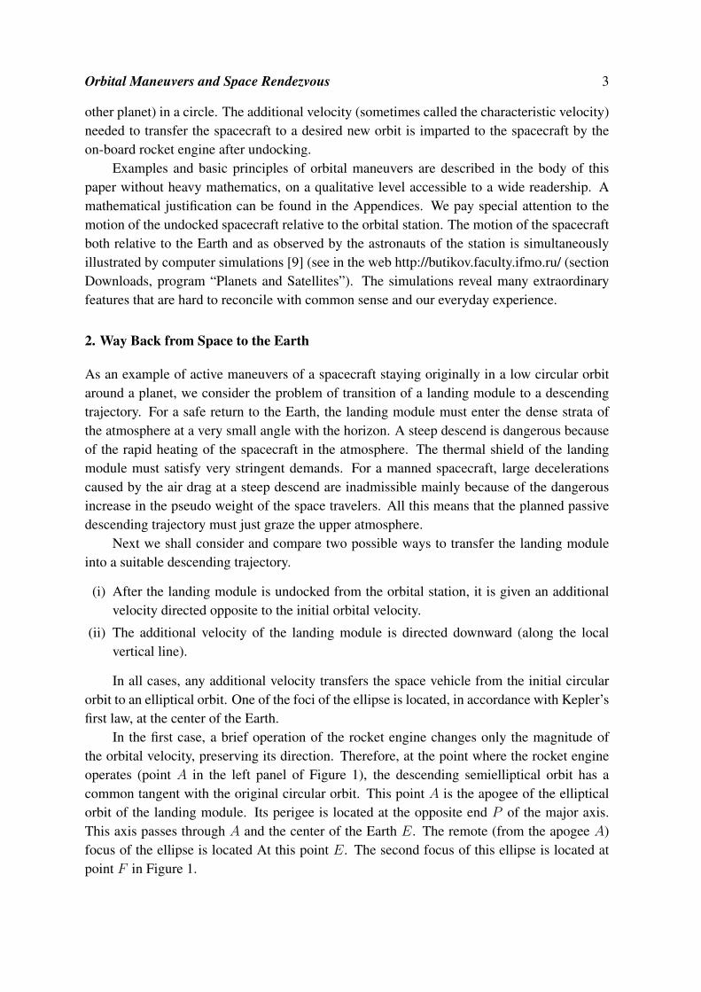
In the first case, a brief operation of the rocket engine changes only the magnitude ofthe orbital velocity, preserving its direction. Therefore, at the point where the rocket engineoperates (point A in the left panel of Figure 1), the descending semielliptical orbit has acommon tangent with the original circular orbit. This point A is the apogee of the ellipticalorbit of the landing module. Its perigee is located at the opposite end P of the major axis.This axis passes through A and the center of the Earth E. The remote (from the apogee A)focus of the ellipse is located At this point E. The second focus of this ellipse is located atpoint F in Figure 1.


S

S

A

P

E

F

LL

v

vcirc

v∆

v∆

A

Figure 1. Descending elliptical trajectory of the landing module after a backward impulseis applied at point A (left), and the descent of the module as it appears to the astronauts onthe orbital station S (right). The thin dotted line shows a conventional upper boundary of theatmosphere.

The additional velocity ∆v must be chosen from the requirement that at point P theellipse must just graze the surface of the planet. More exactly, the ellipse must graze theupper strata of the atmosphere in order the landing module enter the atmosphere at a verysmall angle before reaching this point P of the descending orbit. For this method of landing,the angular distance between the initial point and the point of landing is approximately 180.

The simulation of landing presented in Figure 1 uses one of the programs of the softwarepackage [9]. It is based on numerical integration of the equation of motion of the landingmodule. The simulation shows that the landing module actually moves along the theoreticallypredicted ellipse during almost all first half of revolution around the Earth. But near the pointP its trajectory deviates downward due to the air resistance, which is taken into account inthe simulation. The landing module reaches the ground at point L. To make the influence ofthe air drag more noticeable, the height and density of the atmosphere is exaggerated in thesimulation. A conventional boundary of the atmosphere (whose density reduces exponentiallywith the height over the surface) is shown by the dotted line in Figure 1. At the moment oflanding the station passes through point S of its circular orbit.

The right-hand panel of Figure 1 shows the descent of the module in the frame ofreference associated with the orbital station. At first the landing module actually movesrelative to the station backwards, that is, in the direction of the additional velocity. However,very soon its relative velocity turns downward and reverses. Gradually descending, themodule moves forward and overtakes the station, leaving it far behind. We note that nearthe Earth the trajectory steeply bends towards the surface. This is caused by the increasing airresistance. Due to the same reason, the point of landing occurs before the module reaches theperigee P of the ellipse.

The additional (characteristic) velocity ∆v necessary for the transition from the circular


orbit to this elliptical trajectory can be calculated from the conservation laws of energy andangular momentum. Details of the calculation can be found in Appendix I. We present hereonly the resulting formula:

∆v = vcirc

(1−

√2

1 + r0/R

). (1)

Here vcirc =√GM/r0 =

√gR2/r0 is the circular velocity of the space station, G is the

gravitational constant, M is the mass of the planet, g is the acceleration of free fall, r0 isthe radius of the circular orbit, and R is the Earth’s radius (more exactly, radius of the Earthtogether with the atmosphere).

In the case of a low circular orbit, whose height h = r0 − R over the Earth is smallcompared to the Earth’s radius (h ≪ R), the exact equation, Eq. (1), can be replaced by anapproximate expression:

∆v ≈ vcirch

4R. (2)

For example, if the height h of the circular orbit equals 0.2R ≈ 1270 km, the additionalvelocity ∆v, according to Eq. (2), must be about 5% of the circular velocity. (The calculationon the basis of Eq. (1) with r = R + h = 1.2R gives a more exact value of 4.65%).

S

S

A

P

E

F

LL

v

vcirc

v∆v∆

B

B

Figure 2. Descending elliptical trajectory of the landing module after given a downwardadditional velocity at point B (left), and the descent of the module as it appears to theastronauts on the orbital station S (right).

If the additional velocity imparted to the space vehicle at point B of the initial circularorbit (Figure 2) is directed radially (transverse to the orbital velocity), both the magnitudeand direction of the velocity change. Therefore, the new elliptical orbit intersects the originalcircular one at this point B. For a soft landing, the new elliptical trajectory of the descentmust also graze the Earth (the upper atmosphere) at the perigee P of the ellipse. Using thelaws of energy and angular momentum conservation and requiring that the perigee distance


rP be equal to the Earth’s radius R, we can find (see Appendix I) that the necessary additionalvelocity ∆v for this method of landing is given by

∆v = vcirch

R. (3)

Here vcirc is the circular velocity for the original orbit, h is its height above the surface (abovethe atmosphere), and R is the Earth’s radius (including the atmosphere). Comparing thisexpression with Eq. (2), we see that for this method of transition to the landing trajectory, therequired additional velocity is approximately four times greater than that for the first method.For example, it must equal 20% of the circular velocity, if the height h of the circular orbitis 0.2R. The angular distance between the starting point B and the landing point L (seeFigure 2) for this method equals 90 (a quarter of the revolution), in contrast to the firstmethod, for which the angular distance between the point of transition from the circular orbitto the descending trajectory and the landing point is twice as large (half a revolution).

Figure 2 also shows position S of the orbital station at the moment of landing. We can seethat the station is above and some distance behind the landing module since for the momentof landing the station has not completed a quarter of its revolution beyond the initial point B.

The right-hand side of Figure 2 shows the landing trajectory in the frame of referenceassociated with the orbital station. At first the astronauts on the station see that the landingmodule really moves downward, in the direction of the additional velocity imparted by the on-board rocket engine. However, soon the trajectory bends forward, in the direction of the orbitalmotion of the station. The landing module in its way towards the ground moves forward andovertakes the station, leaving it in its orbital motion far behind.

S

S

A

P

EF

L

L

v

vcirc

v∆v∆

B

B

E

C

Figure 3. Elliptical trajectory of the landing module after acquiring an upward additionalvelocity at point B (left), and the trajectory of the module as it appears to the astronauts on theorbital station S (right).

Strange as it may seem, we can transfer the space vehicle to a landing trajectory by atransverse impulse directed vertically upward as well as downward (Figure 3). In this case,starting from the point B of transition to the elliptical orbit, the landing module first riseshigher above the Earth. Only after it passes through the apogee A of the orbit does it begin


to descend toward point P (the perigee of the orbit), at which it enters the atmosphere. Theangular distance between the starting and the landing points (B and L, respectively) in thiscase equals approximately 270, that is, about three quarters of a revolution. During this time,the orbital station covers almost a whole revolution, and at the moment the vehicle lands atpoint L, the station S is far beyond the landing point.

The trajectory of the landing module as it is seen by the astronauts in the orbital station isshown in the right-hand panel of Figure 3. The module first moves upward, in the direction ofthe additional velocity, but soon turns backward. Its relative motion becomes retrograde, andthe landing module lags behind the station. After circling more than a quarter of the globe inthe retrograde direction, the module’s motion reverses direction. The module then descends,approaching the Earth’s surface tangentially.

For an elliptical orbit that is to graze the Earth, the magnitude of the additional velocitymust be the same for both the downward and upward directions of the impulse. We can easilysee this point either from the laws of the conservation of energy and angular momentum (thecorresponding equations are the same for both cases, see Appendix I), or from considerationsbased on the symmetry between the two cases: for if the goal is to land the module near somepoint P of the Earth’s surface (Figure 2), we must make a transition from the initial circularorbit to an elliptical orbit for which point P is the perigee. The orbits intersect at two pointsB and C. The transition is possible either at B using an upward impulse, or at a symmetricalpoint C using a downward impulse of equal magnitude.

The method of descending from a circular orbit with the help of a backward impulserequires the absolutely minimal amount of rocket fuel. However, this method is very sensitiveto even small variations in the value (and direction) of the additional velocity. In the idealsituation, if the additional velocity has exactly backward direction and the required valuegiven by Eq. (1), the point of landing L is near the perigee P of the ellipse (see Figure 1).During the descent, the landing module covers about one half of the ellipse (from A to P )while the station covers a little less than half its circular orbit. At the moment of landing, thestation is above and a little behind the module (point S in Figure1).

The sensitivity of this method to variations in the additional velocity means that if theactual magnitude of the additional velocity is slightly greater than the required value, the pointof landing L moves considerably from the idealized perigee (point P ) towards the startingpoint A. And if the velocity ∆v is smaller than required, the perigee of the elliptical orbitoccurs above the dense strata of the atmosphere, and the space vehicle may stay in the orbitfor several loops more. Because there is considerable air resistance near perigee, the apogeeof the orbit gradually descends after each revolution. The orbit approaches a low circle.Eventually the space vehicle enters the dense atmosphere and lands. However, it is almostimpossible to predict when and where this landing occurs. To avoid such complications,in practice of orbital flights the additional velocity that transfers the landing module to adescending trajectory is chosen usually to have also a downward transverse component.


3. Transitions between Orbits and Interplanetary Flights

Next we discuss the space maneuvers that can transfer a space vehicle from one circular orbitto another.

Suppose we need to launch a space vehicle from the orbital station into a circular orbitwhose radius is different from that of the space station. After remaining in this new orbit for awhile, the space vehicle is to return to the orbital station and dock to it. What maneuvers mustbe planned to execute this operation? What jet impulses are required for optimal maneuvers?What characteristic velocities must the rocket engine provide?

Designing such transitions between different circular orbits can be related also tointerplanetary space journeys. The orbits of the planets are almost circular, and to a firstapproximation they lie in the same plane. In a sense, planets are stations orbiting thesun. Sending a space vehicle from one planetary orbit to another differs from the problemsuggested above only in that the planets (unlike actual stations) exert a significant gravitationalpull on the space vehicle. But since masses of the planets are small compared to the massof the sun, the gravitational field of a planet is effective only in a relatively small spherecentered at the planet. Outside this sphere of gravitational action of the planet the motion ofa space vehicle (relative to the heliocentric reference frame) is essentially a Keplerian motiongoverned by the sun. In this sense the problem of interplanetary flights is quite similar to theproblem to be discussed here. The only difference is that in the case of interplanetary flightsthe additional velocity needed to simulate a maneuver on the computer should be treated asthe velocity with which the space vehicle leaves the sphere of gravitational action rather thanthe surface of the planet.

Because fuel is critical for all orbital maneuvers, we look first of all at the most fuel-efficient method: the so-called Hohmann’s transfer. In 1925 a German engineer, WalterHohmann, suggested a certain way to transfer between orbits. It is amazing that he wasthinking about this at those old times, many years before launching artificial satellites becametechnically possible. This method uses a semielliptical transfer orbit tangent to the initial andfinal orbits (a semielliptic trajectory that grazes the inner orbit from the outside and the outerorbit from the inside).

As a particular example, we next consider the voyage of a spacecraft from an orbitalstation that moves around a planet in an inner circular orbit of radius r0 to an outer circularorbit of radius 2r0. After remaining in this new orbit for a while, the spacecraft returnsto the orbital station. Figure 4 illustrates the maneuvers. At point P1 the space vehicle isundocked from the station and the on-board rocket engine imparts to the vehicle an additionalvelocity ∆v1 in the direction of the orbital motion. In order to acquire an apogee of 2r0 for thetransitional semielliptic trajectory, the additional velocity ∆v1 must equal 0.1547 vcirc, wherevcirc is the orbital velocity of the station. The calculation of the required additional velocity∆v1 on the basis of the laws of conservation of the energy and angular momentum is given inthe Appendix II. When the space vehicle reaches the apogee (point A1) of the ellipse, a secondtangential impulse ∆v2 is required to increase the velocity from vA to the certain value vc, inorder to place the space vehicle in the outer circular orbit. For this outer orbit, whose radius


SS

A

P

E

F

v

vcirc

v∆v∆

P

vcirc

v∆

A

vAv

P

v∆v∆

v∆

v∆

A

A

v∆

1 1

22

2

2P

v

1

1

1

1

2

c

2

vA

vc

1

2

Figure 4. Semielliptic Hohmann’s transition of a spacecraft to a higher circular orbit withsubsequent return to the orbital station.

is twice the radius r0 of the station orbit, the circular velocity vc equals vcirc/√2, because the

circular velocity is inversely proportional to the square root of the orbit’s radius.An additional velocity of the same magnitude ∆v2 but directed opposite to the orbital

velocity is required to transfer the space vehicle to a semielliptic trajectory that can bring itback to the station. However, when the orbital station is to be the target, another importantconsideration is timing: The station must be in the right spot in its orbit at just the momentwhen the space vehicle arrives. Therefore the instant and the point A2 (see Figure 4) at whichthe maneuver is carried out must be chosen properly in order that the space vehicle reach theperigee P2 simultaneously with the station. To calculate a suitable time, we can use Kepler’sthird law (see Appendix II for details).

To equalize the velocity of the space vehicle with the velocity vcirc of the station as theyboth meet at point P2 (see Figure 4), one more rocket impulse (directed opposite to the orbitalvelocity) is required. It is obvious that now the required additional velocity has the samemagnitude ∆v1 as it does for the very first maneuver.

The right-hand panel of Figure 4 illustrates the motion of the space vehicle in the frameof reference associated with the orbital station. At first the vehicle actually moves forward, inthe direction of the additional velocity ∆v1, but very soon its velocity relative to the station S

turns up and then backward (the relative trajectory makes a small arc near point S). Thefurther motion of the vehicle relative to the station is retrograde. We note that betweenpoints A1 and A2 the space vehicle covers more than one revolution around the station inits retrograde relative motion, while in the planetocentric motion between the correspondingpoints A1 and A2 (left-hand panel of Figure 4) it covers less than one revolution.

4. Rendezvous in Space: Soft Docking to the Space Station

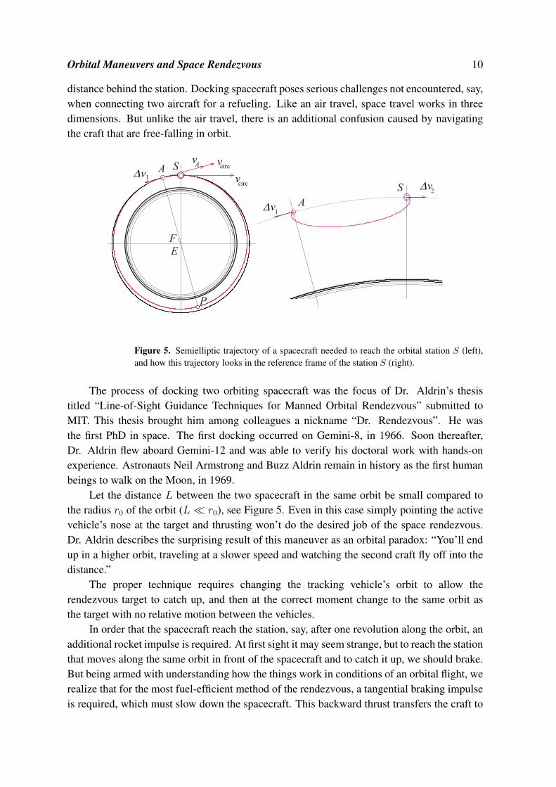
An orbital station S moves around the Earth in a circular orbit (clockwise in Figure 5). Aspacecraft with crew members and supplies is launched to dock to the station, but becauseof an unexpected delay at the launch, the craft moves into the same circular orbit some


distance behind the station. Docking spacecraft poses serious challenges not encountered, say,when connecting two aircraft for a refueling. Like an air travel, space travel works in threedimensions. But unlike the air travel, there is an additional confusion caused by navigatingthe craft that are free-falling in orbit.

S

SA

P

E

vcirc

v∆

vcirc

F

v∆

v∆

1

2

vA

1

A

Figure 5. Semielliptic trajectory of a spacecraft needed to reach the orbital station S (left),and how this trajectory looks in the reference frame of the station S (right).

The process of docking two orbiting spacecraft was the focus of Dr. Aldrin’s thesistitled “Line-of-Sight Guidance Techniques for Manned Orbital Rendezvous” submitted toMIT. This thesis brought him among colleagues a nickname “Dr. Rendezvous”. He wasthe first PhD in space. The first docking occurred on Gemini-8, in 1966. Soon thereafter,Dr. Aldrin flew aboard Gemini-12 and was able to verify his doctoral work with hands-onexperience. Astronauts Neil Armstrong and Buzz Aldrin remain in history as the first humanbeings to walk on the Moon, in 1969.

Let the distance L between the two spacecraft in the same orbit be small compared tothe radius r0 of the orbit (L ≪ r0), see Figure 5. Even in this case simply pointing the activevehicle’s nose at the target and thrusting won’t do the desired job of the space rendezvous.Dr. Aldrin describes the surprising result of this maneuver as an orbital paradox: “You’ll endup in a higher orbit, traveling at a slower speed and watching the second craft fly off into thedistance.”

The proper technique requires changing the tracking vehicle’s orbit to allow therendezvous target to catch up, and then at the correct moment change to the same orbit asthe target with no relative motion between the vehicles.

In order that the spacecraft reach the station, say, after one revolution along the orbit, anadditional rocket impulse is required. At first sight it may seem strange, but to reach the stationthat moves along the same orbit in front of the spacecraft and to catch it up, we should brake.But being armed with understanding how the things work in conditions of an orbital flight, werealize that for the most fuel-efficient method of the rendezvous, a tangential braking impulseis required, which must slow down the spacecraft. This backward thrust transfers the craft to


an inner elliptical orbit (see Figure 5) whose apogee A is at the point of thrust, and perigee atthe opposite point P .

Point A is the only common point of the circular orbit of the station and the ellipticalorbit of the spacecraft. Only at this spatial point the rendezvous is possible. In order thespacecraft arrive at this point simultaneously with the target, the period T of revolution alongthe ellipse must just equal the lapse of time needed for the station to come from point S (whichthe station passed through at the moment of thrust) to point A. We must use this conditionto calculate the required value of the additional velocity ∆v1 for the maneuver. This can bedone by using the conservation laws of energy and angular momentum, and Kepler’s thirdlaw. Details of the calculation can be found in Appendix III. According to Eq. (23), after thebackward thrust the spacecraft must have at point A the following velocity vA:

vA = vcirc

√2− (T0/T )2/3. (4)

Hence the required backward additional velocity ∆v1 can be easily calculated:

∆v1 = vcirc − vA = vcirc

(1−

√2− (T0/T )2/3

). (5)

This is an exact expression for ∆v1. It can be simplified for the case of small distance L

between the tracking vehicle and the target. In this case the elliptical orbit only slightly differsfrom the circular orbit of the station (see Figure 5), so that we can present the required periodas T = T0 − ∆T and consider ∆T/T0 to be a small parameter (∆T/T0 = L/(2πr0) ≪ 1).This yields for vA and ∆v1 instead of Eqs. (4) and (5) the following approximate expressions:

vA ≈ vcirc

(1− 1

3

∆T

T0

), ∆v1 ≈ vcirc

∆T

3T0

. (6)

To illustrate the rendezvous by a computer simulation (see Figure 5), we choose fordefiniteness the angular distance between the spacecraft and the target station to be 15 (thearc AS in Figure 5), so that ∆T/T0 = L/(2πr0) = 1/24. The approximate Eq. (6) yields forthis case ∆v1 = 0.0139 vcirc, while the exact Eq. (5) yields ∆v1 = 0.0145 vcirc (the value usedin the simulation). We see that after one revolution along the ellipse the spacecraft arrives tothe apogee A simultaneously with the station.

The right-hand panel of Figure 5 shows the trajectory of the tracking spacecraft in thereference frame associated with the orbital station. At first the craft’s motion relative to thestation is actually retrograde: it moves backward, in the direction of the additional velocity∆v1. But very soon the relative velocity turns downward and then forward. The vehiclegradually overtakes the station, rises to the initial altitude, and exactly after a revolution occursjust in front of the station. When the craft reaches the station, one more rocket impulse isrequired to equalize their velocities for soft docking. The additional velocity ∆v2 required forthis maneuver must be of the same magnitude as ∆v1, but must be directed oppositely, in thedirection of orbital motion.

If the spacecraft is to approach and dock to the station after two (or n) revolutions alongthe orbit, the characteristic velocity for the maneuver must be approximately twice (or n

times) smaller.


An analytical derivation of the spacecraft trajectory of relative motion in the vicinity ofthe orbital station on the basis of linearized differential equations of motion is presented inAppendix IV.

5. To the Opposite Side of the Orbit and Back

Next we consider one more example of space maneuvers. Imagine we need to launch a spacevehicle from the orbital station into the same circular orbit as that of the station, but there isto be an angular distance of 180 between the vehicle and the station. In other words, they areto orbit in the same circle but at opposite ends of its diameter. How can this be done?

P

S

E

vcirc

F

v∆1

v∆1

A

1

1

P2

A2

vcirc

F2

v∆2

v∆2

ES

V

V

1

1

2

2

1

Figure 6. Transitional geocentric elliptical orbits (outer orbit 1 and inner orbit 2) with periods3/2T0 and 3/4T0, respectively (left), and the corresponding trajectories of relative motion inthe reference frame associated with the orbital station (right).

In order to transfer the space vehicle to the opposite point of the circular orbit, anintermediate elliptical orbit with a definite period of revolution (say, 3/2T0 or 3/4T0) isrequired. To use the first possibility, after undocking from the station, an additional velocity∆v1 must be imparted to the space vehicle in the direction of the orbital motion. Let this bedone at some point P1 (left-hand panel of Figure 6). This velocity ∆v1 appends to the circularvelocity vcirc, and the vehicle starts to move along an outer transitional elliptical orbit 1, whichgrazes the initial circular orbit at perigee P1. Its apogee lies at the opposite point A1.

The period of revolution along this new orbit depends on its major axis P1A1. For ourpurpose, this period must equal 3/2T0, where T0 is the period of the station. If this is the case,the station covers exactly one and a half of its circular orbit during one revolution of the spacevehicle along its elliptical orbit (curve 1 in Figure 6). That is, the space vehicle reaches thecommon point P1 of the two orbits (circular and elliptical) just at the moment when the stationis at the diametrically opposite point of the circular orbit. At this moment the on-board rocketengine must be used for the second time in order to quench the excess velocity of the vehicle.Obviously, the additional velocity of the same magnitude ∆v1 but of the opposite direction isrequired. After this both the station and vehicle move in the same circular orbit being all thetime at the opposite ends of its diameter (say, points S and V in Figure 6).


The right-hand panel of Figure 6 shows the vehicle’s trajectory in its motion relativeto the station (curve 1). Starting to move forward from the station S in the direction ofadditional velocity ∆v1, the vehicle very soon turns upward and then backward. In this frameof reference, almost all its motion from S to final point V is retrograde. After quenching theexcess of velocity over the circular one, the vehicle remains stationary in this frame at theantipodal point V for an indefinitely long time.

To calculate the required value of the additional velocity ∆v1 for the maneuver, we canuse the conservation laws of energy and angular momentum, and Kepler’s third law. Detailsof the calculation can be found in Appendix III. If the period T must equal 3/2T0, velocityat the perigee P1, according to Eq. (23), must be

√2− (2/3)2/3 vcirc = 1.1121 vcirc, whence

∆v1 = 0.1121 vcirc.The second above-mentioned possibility of transition to the opposite side of the circular

orbit requires an inner intermediate elliptical orbit with the period 3/4T0. In the simulationshown in Figure 6 such an orbit is used for the vehicle’s way back to the station. The backwardadditional velocity ∆v2 for the maneuver may be imparted to the vehicle at an arbitrary timemoment, say, when it passes through point A2 (see the left-hand panel of Figure 6). This pointbecomes the apogee of the inner transitional orbit (curve 2). After two revolutions along thisorbit the vehicle meets at this point the station, which covers during this time exactly one anda half revolution along its circular orbit. To equalize velocities of the vehicle and station, onemore thrust of the same magnitude ∆v2 in the direction of orbital motion is required at pointA2. Then soft docking with the station becomes possible.

We note the extraordinary trajectory of vehicle’s motion relative to the station (curve 2on the right-hand panel of Figure 6). The vehicle traces the small loop of this trajectorywhile moving near the apogee A2 of its geocentric orbit after one revolution. The requiredvalue of the vehicle’s velocity at point A2 and of additional velocity ∆v2 for this maneuvercan be calculated with the help of Eq. (23) of Appendix III: the velocity must be equal to√

2− (4/3)2/3 vcirc = 0.8880 vcirc, whence ∆v2 = 0.1120 vcirc. We see that both transitions(through outer and inner elliptical orbits) require almost the same magnitude of the additionalvelocity: ∆v2 ≈ ∆v1.

6. Concluding Remarks

Navigation in space is quite different from what we are used to due to our experience gainedhere on the Earth’s surface. Flying a spacecraft have nothing in common with flying anaircraft. Maneuvers in space are complicated by the free-falling of orbiting bodies in thecentral field of the Earth’s gravity. To design a space mission, we must take into accountthe fundamental laws of physics as they apply to orbital motions. The choice of maneuverssuitable for a specific space flight is restricted by numerous requirements.

In this paper we presented an elementary approach to selection of possible optimalorbital maneuvers for several different space flights. In particular, safe landings of spacecraft,transitions between circular orbits, rendezvous and soft docking of spacecraft with orbitalstations are considered qualitatively. For the most fuel-efficient maneuvers, the additional


velocity must be directed tangentially to the orbital velocity of the vehicle. This conditionprovides Hohmann’s transfers along semielliptic transitional trajectories. The requiredcharacteristic velocities for the maneuvers are calculated with the help of conservation laws.Extraordinary trajectories of the spacecraft relative motion are illustrated by simulations. Therelevant software [9] allows us also to simultaneously observe on the computer screen thespacecraft motion relative to the Earth and relative to the orbital station in a convenient timescale.

Appendix I: Trajectories of a Landing Module

For a safe return to the Earth, a landing module should approach the dense strata of theatmosphere at a very small angle with the horizon. A steep descend is dangerous becauseair resistance causes rapid heating of the module and, in the case of a manned spacecraft,because the astronauts may experience overloads of large g-factors. Therefore the descendingtrajectory should just graze the upper atmosphere.

We calculate here the additional velocity ∆v for two possible impulse maneuvers totransfer the landing module from an initial circular orbit into a suitable descending trajectory:(i) the change in velocity is directed tangentially, antiparallel to the orbital velocity, and (ii)the change in velocity is directed radially, perpendicular to the orbital velocity.

An additional velocity transfers the space vehicle from the initial circular orbit to anelliptical orbit. One of the foci of the ellipse is located, in accordance with Kepler’s first law,at the center of the Earth.

A

P

E

F

vcirc

v∆B

E

F

v

v

A

P

vcirc

A

v∆C

B

Cv

vP

a b

Figure 7. Possible maneuvers to transfer the landing module from a circular orbit to atrajectory grazing the planet: a – by additional velocity directed against the orbital velocity; b– by a transverse additional velocity.

In case (i), the short-term impulse thrust of the rocket engine changes only the magnitudeof the orbital velocity, preserving its direction. Therefore, at the point where the rocket engineoperates (point A in Figure 7, a) the descending elliptical orbit has a common tangent with theoriginal circular orbit. This point A is the apogee of the elliptical orbit. Its perigee is located


at the opposite end P of the major axis, that passes through A and the center of the Earth E.At this point P the ellipse should graze the atmosphere.

To calculate the additional velocity ∆v (the characteristic velocity) that is necessary forthe transition from the circular orbit to this descending elliptical trajectory, we make use ofthe conservation laws for energy and angular momentum.

We let vA = vcirc − ∆v be the velocity at the apogee A of the elliptical orbit (here vcircis the constant velocity in the original circular orbit), and vP be the velocity at the perigee P ,where the ellipse grazes the globe (see Figure 7, a). Then we write the laws of the conservationof energy and angular momentum for these points A and P :

v2A2

− GM

r0=

v2P2

− GM

R; r0vA = RvP . (7)

Here r0 is the radius of the original circular orbit, R is the Earth’s radius (including theatmosphere), and M is the mass of the Earth. Substituting vP from the second equationinto the first, we obtain:

v2A

(1− r20

R2

)=

2GM

r0

(1− r0

R

). (8)

Dividing both parts of Eq. (8) by (1− r0/R), we find the required value vA of the velocity atthe apogee of the elliptical orbit:

vA =

√2GM

r0

1√1 + r0/R

= vcirc

√2

1 + r0/R. (9)

We have expressed the first radical in Eq. (9) in terms of the circular velocity vcirc for theoriginal orbit: vcirc =

√GM/r0. To find the value of the required change in velocity, we

subtract vA from the circular velocity vcirc. This yields for ∆v the cited above expression,Eq. (1), which was used for producing the simulation shown in Figure 1).

In case (ii) the additional velocity imparted to the space vehicle is directed radiallydownward, transversely to the orbital velocity, and both the magnitude and direction of thevelocity change. Therefore the new elliptical orbit intersects the original circular orbit at pointB (see Figure 7, b) at which the additional velocity ∆v is imparted to the landing module. Fora soft landing, the new elliptical trajectory of descent must also graze the Earth (the upperatmosphere) at the perigee P of the ellipse.

The laws of conservation of the energy and the angular momentum for points B and P

in this case can be written as follows:v2circ + (∆v)2

2− GM

r0=

v2P2

− GM

R; vcircr0 = vPR. (10)

Here the velocity vP at the perigee, as well as the additional velocity ∆v, clearly have valuesdifferent from those in Eq. (7). We note that the constant areal (sectorial) velocity in Eq. (10)for the descending elliptical trajectory has the same value as it does for the original circularorbit because an additional radial impulse from the rocket engine does not change the angularmomentum of the landing module.


Substituting vP = vcircr0/R into the first of Eqs. (10) and taking into account thatGM/r0 = v2circ, we get:

(∆v)2 = v2circ

(r0R

− 1)2

. (11)

Next, substituting r0 = R + h in this equation, we finally obtain

∆v = ± h

Rvcirc, (12)

the value given by Eq. (3).The two possible signs in Eq. (12) mean that the additional velocity to the landing module

can be imparted not only downward, but also vertically upward. In both cases the landingmodule will be transferred to the trajectory that just grazes the Earth (see Figure 7, b). It isclear from considerations of symmetry that in both cases the required additional velocity ∆v

has the same magnitude. However, to land on the Earth at the same point P , the upwardimpulse must be imparted to the landing module at a different point of the original circularorbit (point C in Figure 7, b, which is opposite to point B). The angular distance betweenpoint C of the transition to the elliptical orbit and point P of the landing in this case is 270

(three quarter of a revolution). The module at first rises higher. Then, only after it passesthrough the apogee of its elliptical orbit (point A in Figure 7, b), does it begin to descendtowards the Earth’s surface.

Appendix II: Hohmann’s Transitions and Space Rendezvous

The laws of the conservation of energy and angular momentum, together with Kepler’s lawsof motion in a central Newtonian gravitational field, can be used in calculating the maneuversrequired for a planned space flight between two circular orbits, and for an approximatecalculation of an interplanetary flight.

Next we consider a semielliptic Hohmann’s transition between two circular orbits. Weassume for definiteness that we wish to launch a spacecraft from an orbital station that movesaround a planet in a circular orbit of radius r0 into an outer circular orbit of radius, say, 2r0.After the spacecraft remains for some time in this new orbit, it is to return to the stationand dock to it. The simulation experiment for such maneuvers is described in Section 3 (seeFigure 4). Here we present the calculations for the required characteristic velocity and for thetime moments (for the backcount) at which the maneuvers must take place.

The ellipse of the semielliptic transitional trajectory that ensures the most economicaltransition (in expending rocket fuel) grazes both the initial circular orbit (from the outside)and the final circular orbit (from the inside). Hence the perigee distance from the center of theplanet equals r0, the radius of the initial orbit, and the apogee distance equals 2r0, the radiusof the final circular orbit. To calculate the velocity v0 that the spacecraft must have at perigeeof the semielliptic transitional trajectory, we can use Eq. (9), replacing R in it with rA:

v0 = vcirc

√2

1 + r0/rA. (13)


Here rA is the apogee distance of the transitional elliptical orbit from the center of the planet.To find the required additional velocity ∆v1 for the first maneuver, we subtract from v0,Eq. (13), the circular velocity vcirc which the spacecraft already has after undocking fromthe station:

∆v1 = vcirc

(√2

1 + r0/rA− 1

). (14)

Substituting rA = 2r0, we obtain from Eq. (14) ∆v1/vcirc = 2/√3− 1 = 0.1547.

The spacecraft comes to the apogee with a velocity vA, whose value is related to thevelocity v0 at the perigee, Eq. (13), through the law of the conservation of angular momentum(Kepler’s second law):

v0r0 = vArA.

For rA = 2r0 we find, with the help of Eq. (13), vA = v0/2 = 0.577 vcirc. To transferthe spacecraft from the elliptical orbit to the circular orbit of radius 2r0, we must increasethe velocity at apogee by a second jet impulse. The circular velocity in a given centralNewtonian gravitational field is inversely proportional to the square root of the radius of thecircular orbit. For the orbit of radius 2r0, the circular velocity equals vcirc/

√2 = 0.707 vcirc,

where vcirc is the circular velocity for the original orbit of radius r0. Subtracting fromthis value the velocity vA = 0.577 vcirc, at which the spacecraft reaches the apogee ofthe elliptical orbit, we find the additional velocity ∆v2 required for the second maneuver:∆v2/vcirc = 0.707− 0.577 = 0.130.

Next we calculate the time moments at which these maneuvers take place. We can dothis with the help of Kepler’s third law. The semimajor axis a of the elliptical orbit equals(r0+ rA)/2 = (3/2)r0. We call the period of revolution along the original circular orbit (orbitof the station) T0. Then the period for the elliptical orbit equals (a/r0)

3/2 T0 = 1.53/2 T0 =

1.837T0. If we assume t1 = 0 for the first jet impulse, the second jet impulse must beimparted to the spacecraft after a lapse of one-half the period for the elliptical orbit, that is, att2 = 0.9186T0.

During the lapse of time t = t2−t1 taken for the transition, the radius vector of the stationrotates through an angle (2π/T0)t radians. Since the radius vector of the spacecraft turnsduring this semielliptic transition through the angle π, at the instant of the second maneuverthe spacecraft lags behind the station by an angle α = (2π/T0)t − π = 2π(0.9186 − 0.5) =

2π · 0.4186 radians.After the spacecraft remains for a while in its new circular orbit, it is to return to the

orbital station. The optimal return path between the two circular orbits is again semielliptic.The additional velocity ∆v3 in the jet impulse that transfers the spacecraft from the outerorbit to the semielliptic transitional trajectory is directed against the orbital velocity. It isclear from symmetry that in magnitude the additional velocity this time must be exactly thesame as for the preceding transition from the elliptical trajectory to the outer circular orbit,that is, ∆v3 = ∆v2 = 0.130 vcirc. And when the spacecraft reaches the perigee of the ellipticaltrajectory where it grazes the inner circular orbit, one more jet impulse is necessary to quenchthe excess velocity. This time the additional velocity ∆v4 must have the same magnitude


as it does for the first transition from the initial circular orbit to the semielliptic trajectory:∆v4 = ∆v1 = 0.1547 vcirc.

However, the return journey of the spacecraft is complicated by the fact that it is notsufficient to simply transfer the spacecraft to the original inner circular orbit. The spacecraftmust reach the grazing point of the transitional semielliptic trajectory and the inner circularorbit just at the moment when the orbital station arrives at this point. To ensure the rendezvous,we must choose a proper moment for the transition from the outer orbit to the semiellipticreturn path. What should the system configuration be at this moment?

During the direct transition to the outer orbit, the spacecraft lagged behind the station byan angle α = 2π · 0.4186 radians (α is the angle between the radius vectors of the station andthe spacecraft at t = t2). The journey back takes place during the same lapse of time as doesthe journey out. Consequently, in order to meet with the station, the spacecraft must begin itsjourney back at that moment when the station is behind the spacecraft by the same angle α.

Letting T be the period of revolution of the spacecraft along the outer circular orbit, itfollows from Kepler’s third law that T = 23/2 T0 = 2.83T0, since the radius of the outer orbitis 2r0. Calling ∆ω the difference between the angular velocity 2π/T0 of the station and theangular velocity 2π/T of the spacecraft, we have that ∆ω = (2π/T0) · 0.646. The angulardistance β(t) between the station and the spacecraft at an arbitrary time t > t2 is determinedby the expression:

β(t) = ∆ω(t− t2) + α, (15)

since at t = t2 this angular distance equals α. To calculate the time t3 suitable for startingthe return journey, we require that at the moment the station be behind the spacecraft by α.Consequently, the angle β given by Eq. (15) should be made equal to 2πn− α, where n is aninteger:

2πn− α = ∆ω(t3 − t2) + α. (16)

Since α = 2π · 0.4186 radians, we find from Eq. (16) that the time t3 − t2 during whichwe can stay in the outer circular orbit is given by:

t3 − t2 = T0(n− 0.8372)/0.646. (17)

For n = 1 Eq. (17) gives t3 − t2 = 0.252T0. During this interval the spacecraft coversonly a small portion of the outer orbit. And so if the spacecraft is to remain longer, we letn = 2 in Eq. (17) to find that t3 − t2 = 1.7987T0. The period of revolution for the outercircular orbit equals 23/2 T0 = 2.83T0, and so with n = 2 the spacecraft covers a considerablepart of the orbit. If we are satisfied with this duration (otherwise we can take n = 3 ormore, say, n = 4), the third maneuver must be performed at t3 = t2 +1.7987T0 = 2.7174T0.Adding the duration 0.9186T0 of motion along the semielliptic trajectory, we find the momentt4 at which the rendezvous of the spacecraft with the station occurs: t4 = 3.636T0. At thismoment the fourth jet impulse of a magnitude ∆v4 = ∆v1 = 0.1547 vcirc must be imparted tothe spacecraft in order to equalize its velocity with the orbital velocity of the station.

The above discussion illustrates how space maneuvers are calculated using Kepler’s lawsand the laws of conservation of energy and angular momentum. These calculations can be


tested by using the simulation programs [9]. Figure 4 described in Section 3 is obtained bysuch a simulation. It illustrates the particular maneuvers calculated above.

Appendix III: Period of Revolution along an Elliptical Orbit

For some problems of designing a space flight, the crucial issue is the period of revolution ofthe spacecraft along a transitional elliptical orbit. Next we calculate the additional tangentialvelocity that must be imparted to the space probe after its undocking from the station in orderto transfer the craft to an elliptical orbit with the required period of revolution.

We can express this period for the elliptical orbit through the length of its major axis withthe help of Kepler’s third law. Therefore first of all we should find the major axis for a givenvalue of the additional velocity imparted to the spacecraft. Writing down the conservationlaws of energy and angular momentum for the apogee and perigee of the elliptical orbit (likethe orbit shown in Figure 7, a, but with the perigee P not necessarily on the surface), weobtain a relationship between velocity vA at the apogee and distance rP towards the perigee.This relationship is just given by Eq. (8), if we replace R in it with arbitrary distance rP to theperigee:

v2A

(1− r20

r2P

)=

2GM

r0

(1− r0

rP

). (18)

We can find the desired distance from the center of the planet to the perigee, rP , bysolving this quadratic equation. There is no need in reducing it to canonical form and usingthe standard formulas for the roots. Expressing the difference of squares in the left-hand sideof the equation as the product of the corresponding sum and difference, we see at once thatone of the roots is rP = r0. This root corresponds essentially to the initial point (to apogeeA). This irrelevant root appears because one of the conditions used for obtaining the equation,namely that the velocity vector be orthogonal to the radius vector, is satisfied also for the initialpoint (as well as for the perigee).

In order to find the second root, the root that corresponds to the perigee, we divide bothsides of Eq. (18) by (1 − r0/rP ) and express in it 2GM/r0 through the circular velocity(GM/r0 = v2circ) for the initial point A (see Figure 7, a). This yields for the distance rP to theperigee of the orbit:

rP =r0

2(vcirc/v0)2 − 1. (19)

This expression is convenient for determination of parameters of the elliptical orbit in termsof the initial distance r0 and the initial transverse velocity v0.

For the semimajor axis a of the elliptical orbit Eq. (19) yields the following expression:

a =1

2(r0 + rP ) =

r02

1

1− v20/(2v2circ)

. (20)

If the initial velocity equals the circular velocity, that is, if v0 = vcirc, Eq. (20) givesa = r0, since the ellipse becomes a circle, and the semimajor axis coincides with the radiusof the orbit. If v0 →

√2vcirc, that is, if the initial velocity approaches the escape velocity,

Eq. (20) gives a → ∞: the ellipse is elongated without limit. If v0 → 0, equation (20) gives


a → r0/2: as the horizontal initial velocity becomes smaller and smaller, the elliptical orbitshrinks and degenerates into a straight segment connecting the initial point and the center offorce. The foci of this degenerate, flattened ellipse are at the opposite ends of the segment.

Using Eq. (20), we can express the square of the initial velocity v0 of the spacecraft atthe common point of the two orbits in terms of the semimajor axis a:

v20 = v2circ

(2− r0

a

). (21)

Next we can express in Eq. (21) the ratio r0/a in terms of the desired ratio of the periodT0 of the station to the period T of the spacecraft in its elliptical orbit with the semimajor axisa. We do this with the help of Kepler’s third law:

r0a

=

(T0

T

)2/3

. (22)

Hence, to have a desired period T of revolution along a new elliptical orbit after undocking atpoint A (see Figure 7, a), velocity of the spacecraft must be changed by a rocket impulse tothe following value v0:

v0 = vcirc

√2− (T0/T )2/3. (23)

Appendix IV: Approximate Differential Equations for the Relative Motion

Linearized differential equations for the relative motion of orbiting bodies are derived in [10].The non-inertial frame of reference is used whose origin lies in the station. The z-axis of thisframe points perpendicularly to the plane of the orbit; the x-axis lies in the plane of the orbitand extends radially outward, away from the center of the Earth; and the y-axis is parallelto the orbital velocity of the station, vcirc. This frame rotates about z-axis with the angularvelocity Ω = 2π/T0, where T0 is the period of revolution of the station along its circular orbit.

The approximate equations, Eqs. (5) in [10], valid for small spatial distances betweenthe spacecraft and the station (much smaller than the linear dimensions of the orbit), are asfollows:

x = 3Ω2x+ 2Ω y,

y = − 2Ω x, (24)

z = − Ω2 z.

Here x, y, and z are the coordinates that determine the position of the spacecraft relativeto the station, and x, y, and z are the components of the relative velocity. Next we solve theseequations for the situation described in Section 4: the spacecraft initially is in the same circularorbit with the station, but behind it through a small distance L. Assuming t = 0 at the momentof the thrust, we have x(0) = 0, y(0) = −L, z(0) = 0. (see Figure 8). To reach the station(which stays at the origin), the craft at t = 0 gets the initial velocity ∆v = L/(3T0) = LΩ/6π

relative to the station, directed against the orbital velocity: x(0) = 0, y = −∆v, and z = 0.


y

x

-L

A S

Figure 8. Trajectory of the docking spacecraft relative to the orbital station.

For these initial conditions, the particular solution to the system of the linearizedequations of motion, Eqs. (24), can be written as follows:

x(t) =L

3π(cosΩt− 1),

y(t) =L

6π(3Ωt− 4 sinΩt)− L, (25)

z(t) = 0.

We can treat this solution as a periodic motion (with the period T0 = 2π/Ω) of thespacecraft along the ellipse

x(t) =L

3π(cosΩt− 1), y(t) = −2L

3πsinΩt, (26)

whose semiaxes are L/(3π) and 2L/(3π) respectively, with simultaneous uniform motion ofthe ellipse in y-direction with the velocity LΩ/2π = L/T0. During one period T0 the ellipsedisplaces in y-direction (along the orbit) through distance L.

The trajectory given by Eqs. (26) for the time interval 0 < t < T0 is shown in Figure 8.The relative motion of the spacecraft starts at point A, located through distance L behindthe orbital station S, and after the lapse of time T0 = 2π/Ω ends at the origin: the craftapproaches the station S. We can compare this approximate curve with the exact trajectory ofrelative motion shown in the right-hand panel of Figure 5, which is produced by a computersimulation.

[1] Ch. Kittel, W. D. Knight, M. A. Ruderman, Mechanics Berkeley Physics Course, v. 1, New York: McGraw-Hill, 1965.

[2] Space Mission Analysis and Design, 2nd Ed.; Wiley J. Larson & James R. Wertz (editors), Microcosm Inc.,1992.

[3] David Halliday & Robert Resnick, Fundamentals of Physics, John Wiley and Sons Inc., 1974.[4] Jay M. Pasachoff & Marc L. Kutner, W. B., University Astronomy, Saunders Co., 1978.[5] Roger R. Bate, Donald D. Mueller & Jerry E. White, Fundamentals of Astrodynamics; Dover Publications

Inc., 1971.[6] Eugene I. Butikov, Motions of Celestial Bodies: Computer Simulations. IOP Publishing Ltd., 2014.

doi:10.1088/978-0-750-31100-7.[7] Gerald R. Hintz, Orbital Mechanics and Astrodynamics. Techniques and Tools for Space Missions. Springer,

2015[8] Robert A. Braeunig, Rocket and Space Technology.

See in the web <http://www.braeunig.us/space/sources.htm>.[9] E. I. Butikov Planets and Satellites Physics Academic Software (American Institute of Physics), 1999. See

in the web <http://butikov.faculty.ifmo.ru/> (section Downloads).[10] E. I. Butikov, “Relative motion of orbiting bodies,” Am. J. Phys., 69 (1), 63 – 67, 2001.

orbital maneuvers and space rendezvousbutikov.faculty.ifmo.ru/maneuversels.pdf · orbital maneuvers...

Documents