1

Original Article

Analyzing land use change using grid-digitized method

Received 28 May 2013 Accepted 3 Dec. 2013

Orawit Thinnukool, *

Potjamas Chuangchang, and Kittiya Khongkraphan

Department of Mathematics and Computer Science, Faculty of Science and Technology,

Prince of Songkla University, Pattani Campus,

Mueang, Pattani, 94000 Thailand

*Corresponding Author: Tel.: +66 819 0990090; E-mail: orawit.psu@hotmail.com

Abstract

This study aims to analyze land-use change by a digitized-grid method, a simple technique that

can be used for such analysis. We describe a procedure for restructuring land-use data

comprising polygonal “shape files” containing successive (x, y) boundary points of plots for

geographic land-use categories as grid-digitized data, and illustrate this method using data from

Thailand. The new data comprise a rectangular grid of geographical coordinates with land-use

codes and plot identifiers as fields in database tables indexed by the grid coordinates. Having

such a database overcomes difficulties land-use researchers face when querying, analyzing and

forecasting land-use change.

Key words: Land-use, Grid-Digitization, Geographical Information System.

1. Introduction

Land-use is defined as human activity carried out on land (Irwin and Geoghegan, 2001,

Madureira et al., 2007; Rebelo, 2009; Manonmani and Suganya, 2010). Land-use is influenced

by economics, population, culture, politics, and policy. Land-use change is of current scientific

interest due to the massive amounts of data available from remote sensing, widespread use of

global positioning systems, and the availability of geographic information system (GIS)

software. GIS data contain information that needs to be extracted, such as imagery, land

properties, land valuation, and geography (Weng, 2001; Strand et al., 2002; Yang and Qiao,

2010). Google Earth provides free access to current views of the whole surface of the Earth

(Lammeren et al., 2009; Sadr and Rodier, 2012). GIS software is used to develop land-use data,

improve land-use planning (He-bing and Su-xia, 2010; Yang and Qiao, 2010) and to detect land-

use change with image processing based on GIS data (Usha et al., 2012). In addition, scientists

2

study ecological systems (Gret-Regamet et al., 2008) and use GIS technology in environmental

surveys (Gret-Regamey et al., 2008; Manonmani and Suganya, 2010). Klajnsek and Zalik

(2005), Bach et al. (2006), and Mizutani (2009) used GIS data to analyze polygonal shaped land-

use data. They focused on shape change and use polygon events and status to understand land-

use change. Although polygonal data structure can provide thematic maps for displaying patterns

for a given year, the data are difficult to analyze because the polygons change. Bach et al.

(2006), Frazier and Wang (2011), Guo et al. (2011), Hun et al. (2011), and Stehman and

Wickham (2011) described the use of pixels, blocks and polygons to construct accurate maps.

Whiteside et al. (2011) confirmed that pixel-based construction can accurately show land-use

maps.

Using freely available software such as the R program and its special (sp) library, data can be

restructured as points on a grid, for which land-use change is easily measured because the grid

stays put while only the data change. The grid-digitized method provides a data structure that

can be used directly for statistical analysis of land-use change. Data were obtained from the

Department of Land Development, Thailand.

2. Methodology

2.1 Grid-Digitized Method

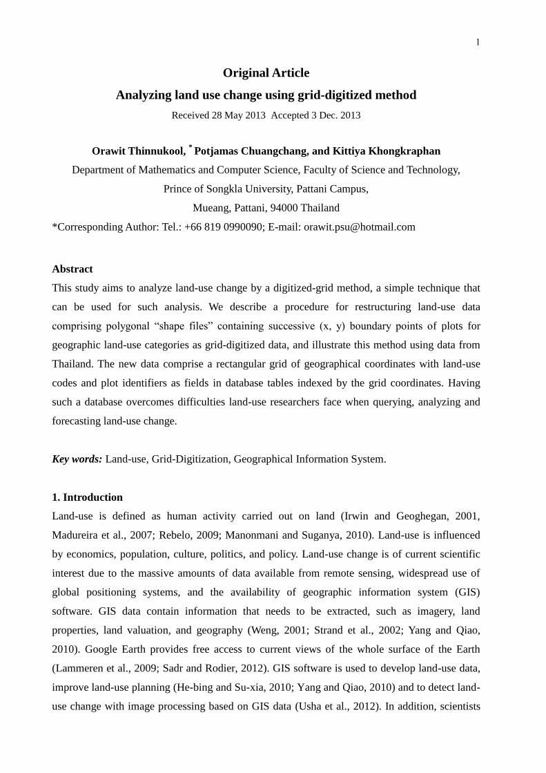
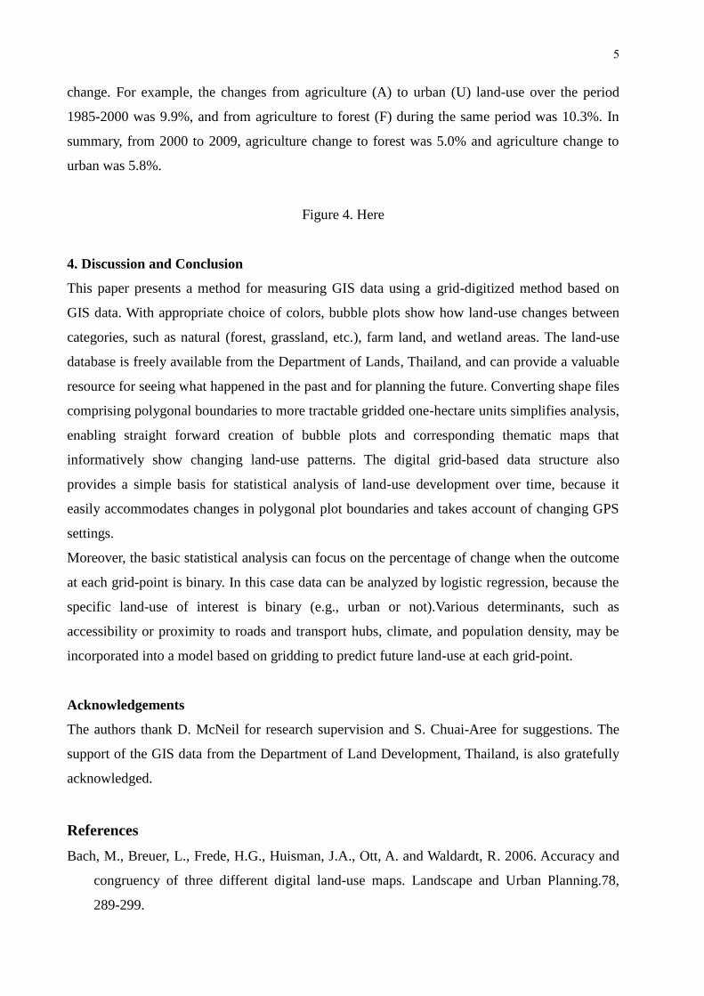
The grid-digitized method involves converting the polygonal data to grid-point data. We

illustrate this method using a simple example as shown in the maps in Figure 1 based on data

structures listed in Table 1.

Figure 1. Here

In this example, the region contains four polygonal plots indentified as 126, 131, 134 and 139,

with corresponding land uses recorded as upland forest, rubber plantation or coconut plantation.

The corresponding data structure is a table with the four fields plotID, pointID, x and y as

indicated in the left panel of Table 1. The pointID field determines the order in which the

boundary points (x,y) are connected to obtain a closed polygon for each land-use plot. For

example the first four and last two values of pointID for plot 134 are indicated in the left-panel

of Figure 1.

Table 1. Here

3

The computational method for connecting from the polygonal coordinates to those based on the

grid involves determining how to assign grid points to polygons. The pseudo code for the

program takes the following form:

for each polygon pi in the specified region

label all grid points inside pi as i

end

This program can be implemented in any language that accommodates for…end loops, provided

this language has a function that determines which elements of a specified set of points are

contained within a specified polygon. We use the R program after loading its sp library, which

contains the function point.in.polygon() (R Development Core Team, 2012). We use R because

we are not aware of any other freely available software that can perform this.

3. Land-Use Data Analysis

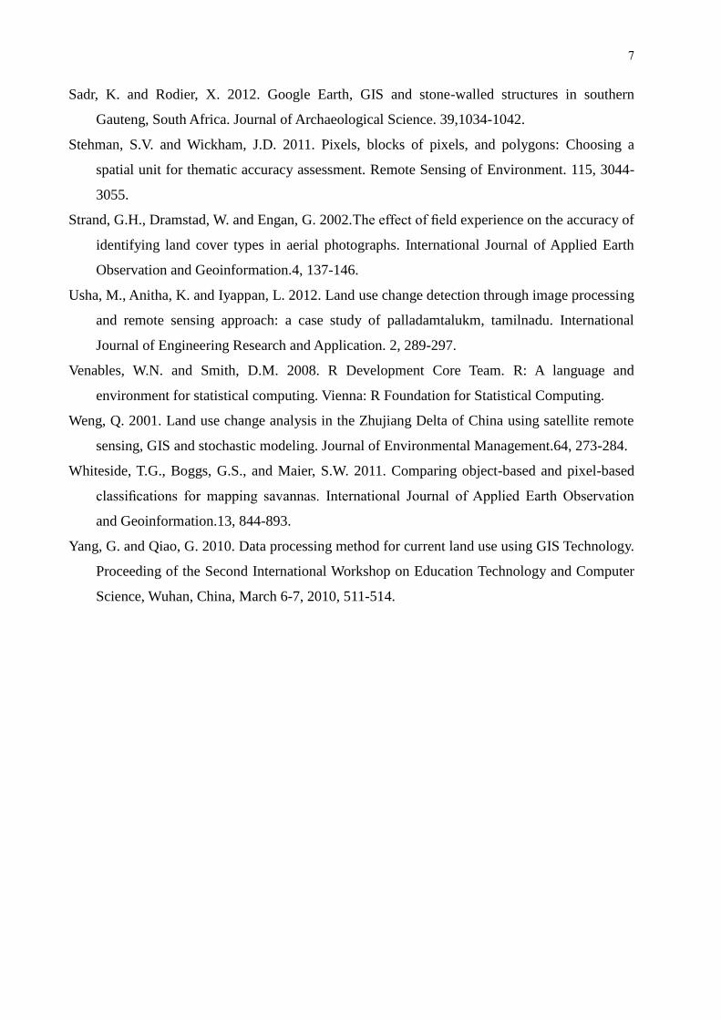
3.1 Land-use change

The grid-digitized method described in the preceding section facilitates measurement of land-use

change. However this measurement is complicated by the fact that land-use codes themselves

change. For example, the categories A2 (rubber plantation), A3 (coconut plantation), and F1

(upland forest) used in 1985 became A302 (para rubber), A405 (coconut plantation) and F101

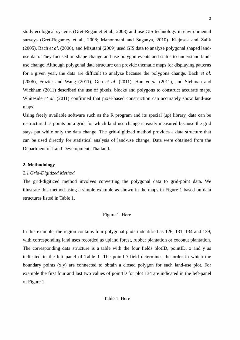
(dense evergreen forest) respectively, in 2009. Using the 2009 land-use codes, Figure 2 shows

the change in land-use for Naka-Yai Island from 1985 to 2009. Note that the four plots

corresponding to the three different land-uses reported in 1985 were reduced to a single land use

in 2009, and this land-use corresponds to F101 in 1985.

Figure 2. Here.

Note that plots 131 and 134 changed from para rubber in 1985 to other land-use in 2009, and

plot 139 also changed completely. An area of plot 126 along its north coast was also lost but

these losses were compensated by gains to plot 126. Note, however, that the apparent loss of the

land along the north coast is not a real loss, because the area remained within the island. The

explanation of this anomaly is that the coordinates shifted, as described next.

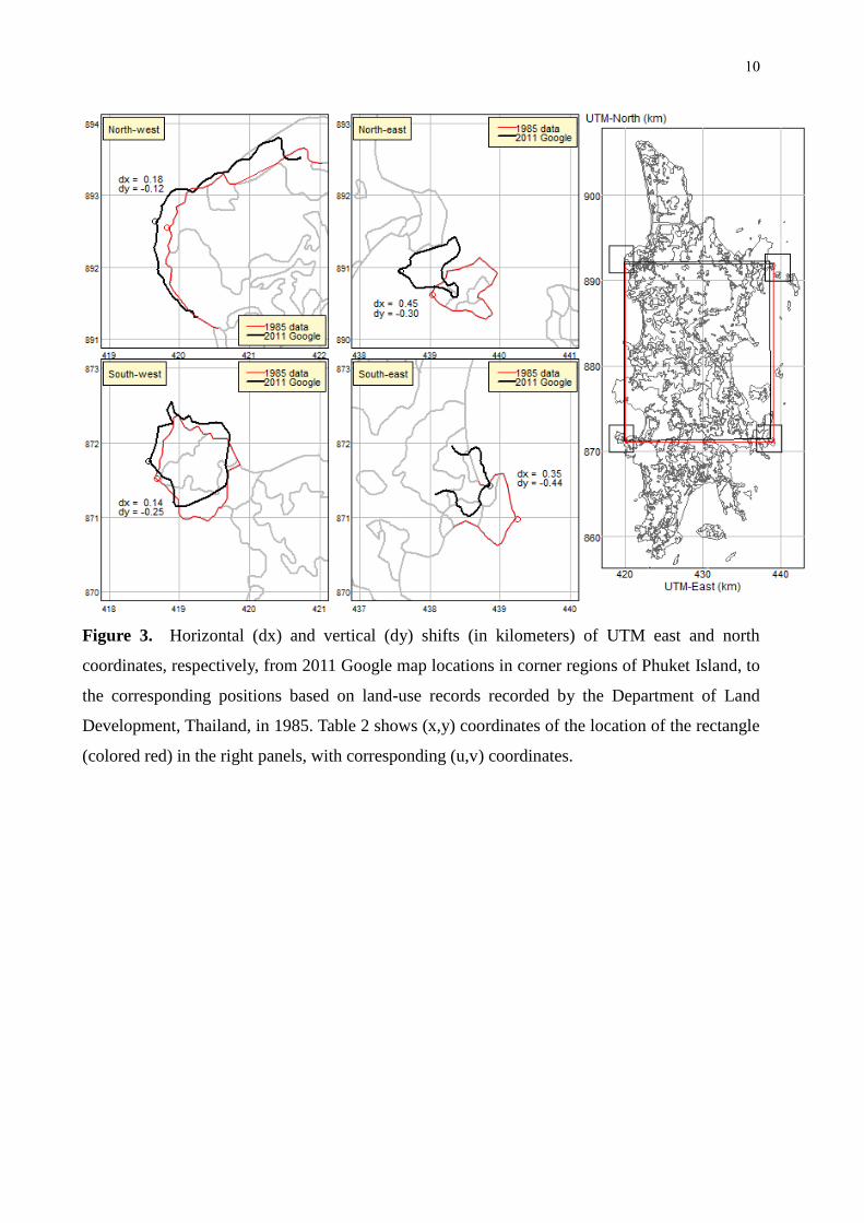
3.2 Coordinate Shifts

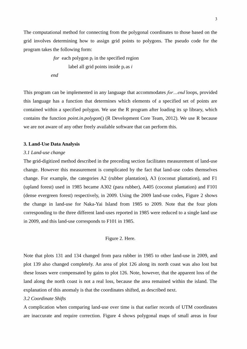
A complication when comparing land-use over time is that earlier records of UTM coordinates

are inaccurate and require correction. Figure 4 shows polygonal maps of small areas in four

4

corners of Phuket province using the original UTM coordinates for 1985 with maps based on

corresponding 2011 Google coordinates (http://maps.google.com) superimposed.

Figure 3. Here

The coordinate shifts illustrated in Figure 3 are quite substantial and complicate accurate

measurement of land-use change. Assuming that coordinates available from Google Earth maps

are correct and that these locations have not changed substantially over recent decades, it is

desirable to convert all land-use coordinates to agree with the corresponding Google Earth

coordinates. Table 2 shows how the coordinates around Phuket Island shifted from 1985 (x, y) to

2009 (u, v)

Table 2. Here

The method we use for this conversion is based on a bilinear transformation of the form.

u = a1 + b1x + c1y+ d1xy (1)

v = a2 + b2x + c2y +d2xy (2)

The parameters (a1, b1, c1, d1, a2, b2, c2, d2) in Equation (1) and (2) are determined by using the

data for the coordinate shifts (dx, dy) at the four locations mapped in Figure 3. There equations

are expressed in matrix form as

g = F h (3)

In this formulation g is the column vector (u1, v1, u2, v2, u3, v3, u4,v4), h is the column vector

(a1, b1, c1, d1, a2, b2, c2, d2) and F is an 8 8 matrix, as follows.

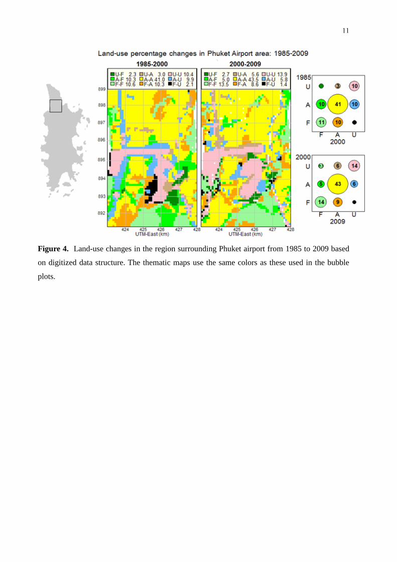
3.3. Analysis Method

Using methods described in the preceding section, the grid-digitized method provides a digital

map. Change in land-use is then summarized in a cross tabulation giving area (in hectares) or

percentages of land-use categories from one period to the next. These numbers can be displayed

as a bubble plot matrix as shown in the right panel of Figure 3, with digital maps of changes

shown in the middle panels. Note that darker colors show changes and lighter colors denote no

5

change. For example, the changes from agriculture (A) to urban (U) land-use over the period

1985-2000 was 9.9%, and from agriculture to forest (F) during the same period was 10.3%. In

summary, from 2000 to 2009, agriculture change to forest was 5.0% and agriculture change to

urban was 5.8%.

Figure 4. Here

4. Discussion and Conclusion

This paper presents a method for measuring GIS data using a grid-digitized method based on

GIS data. With appropriate choice of colors, bubble plots show how land-use changes between

categories, such as natural (forest, grassland, etc.), farm land, and wetland areas. The land-use

database is freely available from the Department of Lands, Thailand, and can provide a valuable

resource for seeing what happened in the past and for planning the future. Converting shape files

comprising polygonal boundaries to more tractable gridded one-hectare units simplifies analysis,

enabling straight forward creation of bubble plots and corresponding thematic maps that

informatively show changing land-use patterns. The digital grid-based data structure also

provides a simple basis for statistical analysis of land-use development over time, because it

easily accommodates changes in polygonal plot boundaries and takes account of changing GPS

settings.

Moreover, the basic statistical analysis can focus on the percentage of change when the outcome

at each grid-point is binary. In this case data can be analyzed by logistic regression, because the

specific land-use of interest is binary (e.g., urban or not).Various determinants, such as

accessibility or proximity to roads and transport hubs, climate, and population density, may be

incorporated into a model based on gridding to predict future land-use at each grid-point.

Acknowledgements

The authors thank D. McNeil for research supervision and S. Chuai-Aree for suggestions. The

support of the GIS data from the Department of Land Development, Thailand, is also gratefully

acknowledged.

References

Bach, M., Breuer, L., Frede, H.G., Huisman, J.A., Ott, A. and Waldardt, R. 2006. Accuracy and

congruency of three different digital land-use maps. Landscape and Urban Planning.78,

289-299.

6

Frazier, A.E. and Wang, L.2011. Characterizing spatial patterns of invasive species using sub-

pixel classifications. Remote Sensing of Environment. 115, 1997-2007.

Gret-Regamey, A., Bebi, P., Bishop, I.D. and Schmid, W.A. 2008. Linking GIS-based model to

value ecosystem services in an Alpine region. Journal of Environment Management. 89,

197-208.

Guo, L., Du, S., Haining, R. and Zhang, L. 2011. Global and local indicators of spatial

association between points and polygons: A study of land use change. International Journal

of Applied Earth Observation and Geoinformation. 21, 384-356.

He-bing, Z. and Su-xia, Z. 2010. Development and application of land-use planning

management information system based on ArcGIS. Proceedings of 2010 International

Forum on Technology and Application, Kunming, China, July 16-18, 2010, 64-67.

Huh, Y., Yu, K., and Heo, J. 2011. Detecting conjugate-point pairs for map alignment between

two polygon data sets. Computer Environment and Urban System. 35, 250-262.

Irwin, E.G. and Geoghegan, J. 2001. Theory, data, methods: developing spatially explicit

economic models of land use change. Agriculture, Ecosystem and Environment. 85, 7-23.

Klajnsek, G. and Zalik, B. 2005. Merging polygon with uncertain boundaries. Computer and

Geosciences. 31, 353-359.

Lammeren, R.V., Houtkamp, J., Colijn, C., Hiferink, M. and Bouwman, A. 2009. Google Earth

based visualization of Land Use scenario studies. Proceeding of GSDI 11 World

Conference: Spatial Data Infrastructure Convergence: Building SDI Bridges to Address

Global Challenges, Rotterdam, The Netherlands. June 15-19, 2009.

Madureira, L., Rambonilaza, T. and Karpinski, I. 2007. Review of methods and evidence for

economic valuation of agricultural on-commodity outputs and suggestions to facilitate its

application to broader decisional contexts, Agriculture, Ecosystems and Environment. 120,

5-20.

Manonmani, R. and Suganya, M.D. 2010. Remote sensing and GIS application. In Change

detection study in urban zone using multi temporal satellite. International Journal of

Geomatics and Geosciences.1, 60-65.

Mizutani, C.2009. Land use transition process analysis using polygon events and polygon status:

A case study of Tsukuba science city. Proceedings of the 17th International Conference of

Geoinformatics, Virginia, U.S.A., August 12-14, 2009, 1-6.

Rebelo, E.M. 2009. Land-economic rent computation for urban planning and fiscal purposes.

Land Use Policy. 26, 521-534.

7

Sadr, K. and Rodier, X. 2012. Google Earth, GIS and stone-walled structures in southern

Gauteng, South Africa. Journal of Archaeological Science. 39,1034-1042.

Stehman, S.V. and Wickham, J.D. 2011. Pixels, blocks of pixels, and polygons: Choosing a

spatial unit for thematic accuracy assessment. Remote Sensing of Environment. 115, 3044-

3055.

Strand, G.H., Dramstad, W. and Engan, G. 2002.The effect of field experience on the accuracy of

identifying land cover types in aerial photographs. International Journal of Applied Earth

Observation and Geoinformation.4, 137-146.

Usha, M., Anitha, K. and Iyappan, L. 2012. Land use change detection through image processing

and remote sensing approach: a case study of palladamtalukm, tamilnadu. International

Journal of Engineering Research and Application. 2, 289-297.

Venables, W.N. and Smith, D.M. 2008. R Development Core Team. R: A language and

environment for statistical computing. Vienna: R Foundation for Statistical Computing.

Weng, Q. 2001. Land use change analysis in the Zhujiang Delta of China using satellite remote

sensing, GIS and stochastic modeling. Journal of Environmental Management.64, 273-284.

Whiteside, T.G., Boggs, G.S., and Maier, S.W. 2011. Comparing object-based and pixel-based

classifications for mapping savannas. International Journal of Applied Earth Observation

and Geoinformation.13, 844-893.

Yang, G. and Qiao, G. 2010. Data processing method for current land use using GIS Technology.

Proceeding of the Second International Workshop on Education Technology and Computer

Science, Wuhan, China, March 6-7, 2010, 511-514.

8

Figure 1. Conversion of polygonal representation (left panel) to digital representation (right

panel) for land-use data from Naka-Yai Island in Phuket Province of Thailand in 1985.

9

Figure 2. Land-use change in Naka-Yai Island from 1985 to 2009 with losses from 1985 (upper

right panel) and gains to 2009 (lower right panel).

10

Figure 3. Horizontal (dx) and vertical (dy) shifts (in kilometers) of UTM east and north

coordinates, respectively, from 2011 Google map locations in corner regions of Phuket Island, to

the corresponding positions based on land-use records recorded by the Department of Land

Development, Thailand, in 1985. Table 2 shows (x,y) coordinates of the location of the rectangle

(colored red) in the right panels, with corresponding (u,v) coordinates.

11

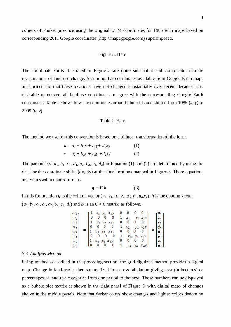
Figure 4. Land-use changes in the region surrounding Phuket airport from 1985 to 2009 based

on digitized data structure. The thematic maps use the same colors as these used in the bubble

plots.

12

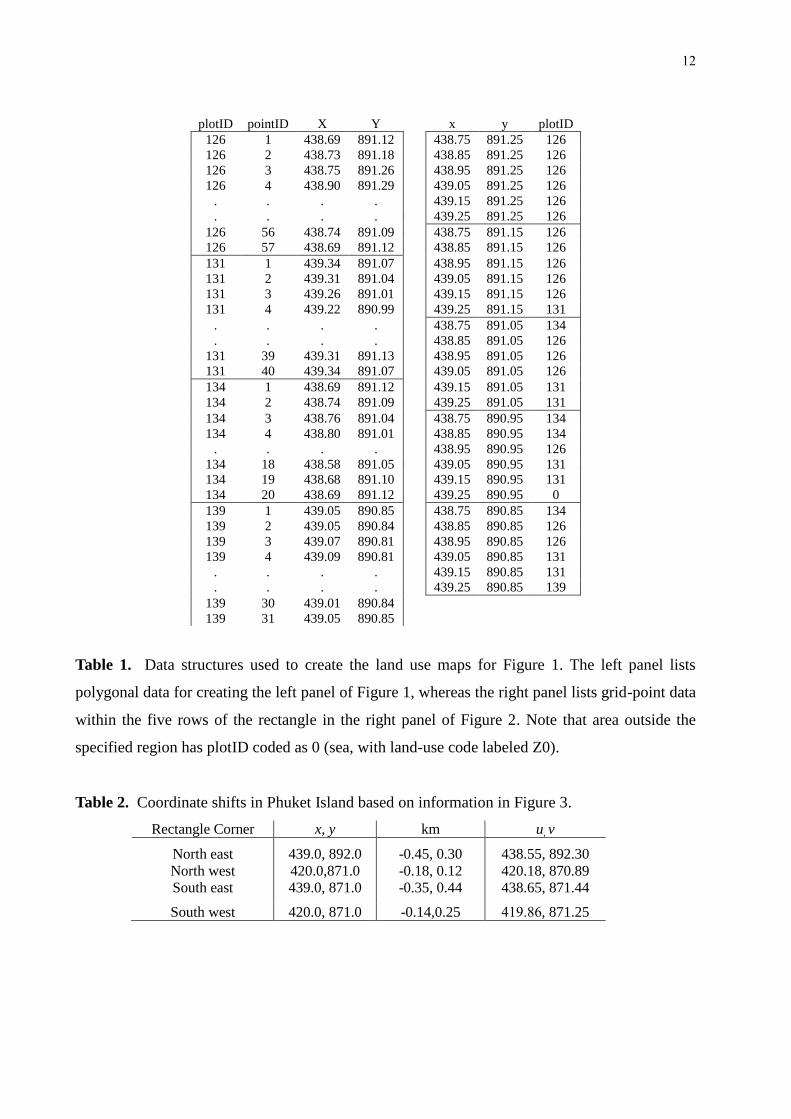
Table 1. Data structures used to create the land use maps for Figure 1. The left panel lists

polygonal data for creating the left panel of Figure 1, whereas the right panel lists grid-point data

within the five rows of the rectangle in the right panel of Figure 2. Note that area outside the

specified region has plotID coded as 0 (sea, with land-use code labeled Z0).

Table 2. Coordinate shifts in Phuket Island based on information in Figure 3.

Rectangle Corner x, y km u, v

North east

North west

South east

439.0, 892.0

420.0,871.0

439.0, 871.0

-0.45, 0.30

-0.18, 0.12

-0.35, 0.44

438.55, 892.30

420.18, 870.89

438.65, 871.44

South west 420.0, 871.0 -0.14,0.25 419.86, 871.25

plotID pointID X Y x y plotID

126 1 438.69 891.12 438.75 891.25 126

126 2 438.73 891.18 438.85 891.25 126

126 3 438.75 891.26 438.95 891.25 126

126 4 438.90 891.29 439.05 891.25 126

. . . . 439.15 891.25 126

. . . . 439.25 891.25 126

126 56 438.74 891.09 438.75 891.15 126

126 57 438.69 891.12 438.85 891.15 126

131 1 439.34 891.07 438.95 891.15 126

131 2 439.31 891.04 439.05 891.15 126

131 3 439.26 891.01 439.15 891.15 126

131 4 439.22 890.99 439.25 891.15 131

. . . . 438.75 891.05 134

. . . . 438.85 891.05 126

131 39 439.31 891.13 438.95 891.05 126

131 40 439.34 891.07 439.05 891.05 126

134 1 438.69 891.12 439.15 891.05 131

134 2 438.74 891.09 439.25 891.05 131

134 3 438.76 891.04 438.75 890.95 134

134 4 438.80 891.01 438.85 890.95 134

. . . . 438.95 890.95 126

134 18 438.58 891.05 439.05 890.95 131

134 19 438.68 891.10 439.15 890.95 131

134 20 438.69 891.12 439.25 890.95 0

139 1 439.05 890.85 438.75 890.85 134

139 2 439.05 890.84 438.85 890.85 126

139 3 439.07 890.81 438.95 890.85 126

139 4 439.09 890.81 439.05 890.85 131

. . . . 439.15 890.85 131

. . . . 439.25 890.85 139

139 30 439.01 890.84

139 31 439.05 890.85