originally published as: milsch, h., blöcher, g

Originally published as Milsch H Bloumlcher G Engelmann S (2008) The relationship between hydraulic and electrical transport properties in sandstones An experimental evaluation of several scaling models - Earth and Planetary Science Letters 275 3-4 355-363 DOI 101016jepsl200808031

The relationship between hydraulic and electrical transport properties in sandstones An experimental evaluation of several scaling models

Harald Milsch1 Guido Bloumlcher1 and Silvio Engelmann1 2

1Deutsches GeoForschungsZentrum Telegrafenberg D-14473 Potsdam Germany milschgfz-potsdamde2Technische Universitaumlt Berlin Institut fuumlr Angewandte Geowissenschaften Ackerstr 76 D-13355 Berlin Germany

Abstract

The purpose of this paper is to investigate the relationship between the parameters that define the hydraulic and electrical transport in porous rock We therefore measured the effective pressure dependence of both permeability (k) and (specific) electrical conductivity (σ) of three different types of sandstones (Fontainebleau Flechtinger and Eberswalder) The experiments were performed in a high pressure and high temperature (HPT) permeameter at a maximum confining- and pore pressure of 50 MPa and 45 MPa respectively and a constant temperature of 40degC 01 molar NaCl-brine was used as the pore fluid We show that for the present rock-fluid combinations surface conductivity can be neglected The experiments were complemented with 2D image analysis and mercury porosimetry to derive the average pore radii the specific inner pore surfaces and the pore radius distributions of the samples The experimental and microstructural results were used to relate both transport properties by means of different length scales and to test the associated scaling models based on (1) the equivalent channel concept (2) statistics and percolation and (3) an interpretation of mercury porosimetry data As the principal result none of these integrated models could adequately reproduce the respective transport property within experimental error margins Furthermore it is emphasized that these models are not applicable for effective pressures other than zero unless the concurrent evolution of the microstructure respectively the length scale can be characterized By comparison it is shown that purely empirical permeability-conductivity relationships can always be adjusted to provide a reasonable description of the coupled k-σdependence on effective pressure However it is implied that the included empirical length parameter is fundamentally different from the ones above as it is a pressure independent constant that contains no true microstructural or physical information

Key Words

permeability electrical conductivity transport properties petrophysics scaling models sandstone

Title Page

1 Introduction1

Both permeability (k) and (specific) electrical conductivity (σ) are important rock 2

transport properties whose determination is of uppermost interest in all areas where the 3

characterization of fluid flow within a pore space is the key issue For example forecasts on 4

the productivity of hydrocarbon and geothermal reservoirs require a reliable estimate of the 5

permeability of the constituent rocks Both parameters are measured as bulk properties but are 6

in fact defined by the individual pore structure of a rock This is evident for permeability but 7

is also true for the electrical conductivity as long as the latter is governed by the conductivity 8

of a fluid within the pore space in other words as long as surface conductivity can be 9

neglected Furthermore the pore structure is affected by changes in the state of stress acting 10

on the rock Both transport properties are therefore dependent on effective stress or in the 11

lithostatic (isotropic) case on effective pressure (peff) In the present study the term ldquoeffective 12

pressurerdquo is defined as the difference between confining- (pc) and pore pressure (pp) according 13

to Terzaghirsquos Principle (peff = pc - pp Terzaghi 1923) It is thus synonymously used with the 14

term ldquodifferential pressurerdquo Compared to permeability electrical rock conductivity is 15

significantly easier to measure both in the lab and in situ Thus not least for practical reasons 16

it is desirable to establish a link between both transport properties and to couple both 17

parameters through microstructure-related length scales18

Such approaches have been made repeatedly during the last five decades (eg Wyllie 19

and Rose 1950 Walsh and Brace 1984 Johnson et al 1986 Katz and Thompson 1986 20

1987 Gueacuteguen and Dienes 1989 Avellaneda and Torquato 1991 Martys and Garboczi 21

1992) The strategy applied in these models is first to set up independent expressions for 22

both hydraulic and electrical transport as a function of the pore space microstructure The rock 23

permeability (k) and the specific electrical rock conductivity (σ) are defined by the Darcy 24

Equation (Eq 1 Darcy 1856) and Ohmrsquos Law (Eq 2 Ohm 1826) respectively25

26

Main Text

pq η

k (1)27

28

VJ σ (2)29

30

where q η p J and V denote the fluid volume flux the dynamic fluid viscosity the 31

pressure gradient the current flux density and the potential gradient respectively These 32

equations are then related to the microstructural information by means of geometrical 33

(equivalent channel) models (Wyllie and Rose 1950 Paterson 1983 Walsh and Brace 1984) 34

as well as statistical and percolation concepts (Katz and Thompson 1986 1987 Gueacuteguen and 35

Dienes 1989) The two independent expressions are finally joined together to yield a 36

relationship (Eq 3) that links both transport properties where the electrical conductivity is 37

expressed in terms of the formation factor (F)38

39

FLck

12 (3)40

41

where c and L denote a shape factor and a characteristic length scale respectively The 42

formation factor F here is defined as the ratio between the electrical conductivity of the fluid 43

(σfl) at the respective experimental temperature and the measured conductivity of the rock (σ)44

The related assumption that in the present study surface conductivity can be neglected with 45

respect to the brine conductivity is reasonable as outlined in Section 22 46

In other approaches Eq 3 is introduced in an ad hoc manner and L is derived by 47

physical considerations like Joule dissipation and electrically weighted pore surface-to-48

volume ratios (Johnson et al 1986) or nuclear magnetic resonance (NMR) relaxation times 49

(Avellaneda and Torquato 1991)50

The physical meaning of both parameters c and L is therefore dependent on the 51

respective model and can vary significantly It is thus crucial for the validity of a model that 52

the characteristic length scale L is appropriately defined and determined as it has to contain all 53

the microstructural information needed to characterize the interrelationship between both 54

transport properties55

The purpose of this paper is to test the predictions of Eq 3 against original 56

experimental and microstructural data obtained for three different types of sandstone 57

described in Section 21 More specifically we test the models proposed by Walsh and Brace 58

(1984) Gueacuteguen and Dienes (1989) and Katz and Thompson (1986 1987) with shape factors 59

(c) and length scales (L) listed in Table 1 60

Furthermore we compare Eq 3 with an established empirical relationship between k61

and F (Eq 4 eg Brace 1977 Walsh and Brace 1984 and references cited therein) that has 62

been obtained from investigations on the pressure dependence of the coupled transport 63

properties64

65

rFLck E

12 (4)66

67

where r denotes an empirical rock dependent parameter following the notation in Walsh and 68

Brace (1984) The subscript E has been introduced to distinguish between both length scales 69

defined within the respective relationship 70

Section 2 outlines the experimental and microstructural procedures applied In Section 71

3 the results obtained from both investigations are presented and the comparison between 72

original data and the predictions of the scaling models is performed In Section 4 the outcome 73

is analysed in detail for each of the models tested This section also emphasizes the 74

conceptual difference between physical (Eq 3) and empirical (Eq 4) k-F relationships 75

Section 5 summarized the principal findings of this study by means of some concluding 76

remarks 77

78

2 Experimental and Microstructural Methodology79

21 Sample Material and Fluid80

For the experiments three different types of sandstone samples were chosen (1) 81

Fontainebleau sandstone a pure quartz arenite quarried from an outcrop near Fontainebleau 82

France This rock has extensively been used in previous studies aiming at the morphology and 83

physical properties of sandstones (eg David et al 1993 Auzerais et al 1996 Coker et al 84

1996 Cooper et al 2000) (2) Flechtinger sandstone a Lower Permian (Rotliegend) 85

sedimentary rock quarried from an outcrop near Flechtingen Germany (3) Eberswalder 86

sandstone a Lower Permian (Rotliegend) rock cored during drilling of a prospective gas well 87

(Eb276) at Eberswalde Germany The two Rotliegend samples are arcosic litharenites 88

containing varying amounts of quartz (55 ndash 65 ) feldspars (15 ndash 20 ) and rock fragments 89

mainly of volcanic origin (20 ndash 25 ) In addition smaller amounts of clays are present 90

predominantly illite and chlorite The specimens were cylindrical in shape having a diameter 91

of 30 mm and a length of 40 mm (Fontainebleau and Flechtinger) or 383 mm (Eberswalder)92

The dry mass of the specimens was 6925 g (Fontainebleau) 6836 g (Flechtinger) and 6754 93

g (Eberswalder) 94

To enable electrical conductivity measurements 01 molar NaCl-solution was used as 95

the pore fluid The electrical conductivity of this fluid (σfl) at 25degC is 108 mScm and was 96

measured with a hand held conductivity meter (WTW Multi 340i with TetraCon 325 97

conductivity probe) Prior to setting up the specimen assembly the samples were vacuum-98

saturated with this fluid The comparison between both dry and wet sample mass yields the 99

fluid mass within the (connected) pore space thus the (connected) pore volume and finally 100

the (connected) porosity (φs) The density of the fluid at 20degC and ambient pressure was 101

assumed to be equal to that of pure water (0998 gcm3) 102

103

22 Experimental Procedure104

The experiments were performed in a recently set up HPT-permeameter described in 105

detail in Milsch et al (2008) To avoid disturbance of the measurement by room temperature 106

fluctuations the experimental temperature was maintained at 40 (plusmn 1) degC 107

The dynamic viscosity of the fluid at this temperature is 6534 microPa s at a pressure of 5 108

MPa and was calculated with the NIST program REFPROP again assuming pure water 109

properties The electrical conductivity of the fluid at this temperature is 141 mScm and was 110

determined in previous temperature stepping experiments yielding a linear temperature 111

coefficient of approximately 002degC By comparison we found an excellent agreement with 112

the data in Revil et al (1998) (regarding the temperature coefficient) as well as the predictions 113

of the Arps-Equation (Arps 1953) and the experimental data in Sen and Goode (1992) 114

(regarding the fluid conductivity itself) 115

In connection with the definition of the formation factor in Section 1 similar 116

experiments with fluids of varying salt content implied that a contribution from surface 117

conductivity to the actual overall sample conductivity was small even for the Rotliegend 118

samples containing minor amounts of clays For the Fontainebleau sandstone this in 119

agreement with the observations made by David et al (1993) Surface conductivity has thus 120

reasonably been neglected for all samples tested in this study The supporting data is 121

presented as part of the supplementary material (file ldquoSurface Conductivitydocrdquo) 122

The sample permeability (k) was measured with a steady state method making direct 123

use of Darcyrsquos Law The electrical conductivity (σ) was determined in a four-electrode 124

arrangement with a variable shunt resistor and silver paint rims at the samples as potential 125

electrodes (see Milsch et al 2008 for more details on both methodologies) Both transport 126

properties were measured simultaneously To investigate the relative changes of both 127

parameters effective pressure ramping was performed by successively increasing and 128

decreasing both confining and pore pressure The pressures were varied from 10 to 50 MPa 129

(pc) and 5 to 45 MPa (pp) respectively Three full cycles and thus 12 individual ramps were 130

conducted for each sample In contrast to electrical conductivity which can be determined 131

continuously during pressure ramping permeability measurements have to be performed 132

stepwise Depending on the sample permeability 5 to 10 measurements have been taken along 133

each ramp at effective pressure intervals ranging from 25 to 15 MPa134

135

23 Microstructural Methodology136

Subsequent to each test thin sections were prepared Two on the opposing faces of the 137

specimen and one along the core The sections were saturated with blue epoxy to allow 2D 138

image analysis to be performed on binary images (Zeiss Axioplan with Axiocam and KSRun) 139

For a significant statistics approximately 1000 pores were evaluated for each section in two 140

different magnifications of 25x and 100x Among a variety of other pore structural parameters 141

the image analysis program yields the measured pore radius distribution as a function of the 142

(total) cumulative porosity as well as an average pore radius The minimum resolvable pore 143

radius is defined by the analysis program and is dependent on the magnification chosen 65 144

microm at 25x and 17 microm at 100x A description of the image analysis procedure has been placed 145

into the supplementary materials section (file ldquoImage Analysisdocrdquo)146

In addition mercury porosimetry (WS2000 Fisons Instruments) was performed after 147

the experiments on broken parts of the samples having a volume of approximately 1 to 2 cm3148

each Mercury porosimetry assumes a local cylindrical geometry for all parameters derived 149

and is based on the intrusion of a non-wetting fluid (Hg) at a progressively increased pressure 150

of up to 200 MPa and application of the Washburn Equation pcap = -4γcosθd where pcap is 151

the capillary pressure γ is the surface tension (485 mNm) θ is the contact angle (1413deg) and 152

d is the local diameter of the pore space (eg Van Brakel et al 1981) This independent 153

method also yields a pore radius distribution of the samples as a function of the (connected) 154

cumulative porosity as well as an average pore radius In addition the specific inner surface 155

distribution is calculated from the mercury injection curve In contrast to 2D image analysis 156

the pore radius in that case designates the throat radius that relates to an individual injection 157

pressure The minimum resolvable pore radius (at 200 MPa maximum injection pressure) is 158

37 nm 159

160

3 Results161

31 Experiments162

Table 2 displays an overview of the experimental sample properties permeability (k0) 163

and electrical conductivity (σ0) at starting conditions which were a confining pressure of 10 164

MPa a pore pressure of 5 MPa and a temperature of 40degC The formation factor of the 165

samples (F0) is shown in addition The porosity (φs) has been determined at ambient 166

conditions by fluid saturation as described above One notices that the Fontainebleau 167

sandstone does not follow the parameter systematics of the two Rotliegend samples implying 168

significant differences in morphology It has a significantly higher permeability at the lowest 169

conductivity and an intermediate porosity It is also worth to note that in the present case a 170

variation in permeability over three orders of magnitude relates only to a variation in 171

conductivity by a factor of approximately three 172

To present the dependence of the respective transport property on effective pressure 173

for all three samples in one figure it is convenient to perform a normalization with its starting 174

value (k0 or σ0) Figure 1a and 1b show the measured normalized permeability and electrical 175

conductivity respectively as a function of effective pressure Absolute values can then be 176

obtained from the respective figure and Table 2 For each of the rocks the figures display an 177

average of all measurements taken during effective pressure ramping The related error 178

margins regarding the maximum upper and lower departure from the mean are discussed in 179

Section 33 Both transport properties are sensitive to changes in effective pressure The 180

sensitivity increases from the Fontainebleau over the Flechtinger to the Eberswalder 181

sandstone Furthermore for all sandstones the sensitivity decreases with increasing effective 182

pressure The percental changes of both transport properties are closely related for the 183

Fontainebleau and the Flechtinger sandstones In contrast for the Eberswalder sandstone the 184

decrease in permeability at lower effective pressures is significantly more pronounced than 185

the decrease in electrical conductivity The respective approximately linear or bilinear 186

dependence becomes evident when the normalized permeability is displayed as a function of 187

the normalized electrical conductivity (Figure 1c) 188

189

32 Microstructure190

The principal results of the microstructural investigations with 2D image analysis and 191

mercury porosimetry are compiled in Table 3 The porosities determined with 2D image 192

analysis (φ2D) are strongly dependent on the chosen magnification of the microscope This 193

could be due to cutting effects at the edges of the binary image becoming more important at 194

greater magnifications or resolution deficites at smaller magnifications Depending on the 195

magnification the porosities also significantly differ from the ones obtained by both fluid 196

saturation (φs) and mercury porosimetry (φHg) In contrast φs and φHg are always in rather 197

good agreement The reliability of these (connected) porosities is supported by a comparison 198

of the Fontainbleau dry bulk density with the density of quartz The (total) porosity value so 199

obtained (75 ) is in excellent agreement with the two others 200

The table clearly indicates the differences in the average pore radii obtained by both 201

methods Naturally the average pore throat (rAHg) is significantly smaller than the pore itself 202

(rA2D) In both cases the average pore radius decreases from the Fontainebleau over the 203

Flechtinger to the Eberswalder sandstone In contrast the specific inner surface (AHg) of the 204

Fontainebleau sandstone is significantly smaller than the ones of the two Rotliegend samples 205

The pore radius distribution from mercury porosimetry (Figure 2a) indicates that is due to the 206

rather discrete and large pore radius of the Fontainebleau sandstone This contrasts the 207

distribution of the two Rotliegend samples implying significant morphological differences 208

Their larger specific inner surfaces (Figure 2b) are principally due to contributions from pore 209

radii between 02 ndash 20 microm210

Assuming a cylindrical geometry the specific inner surface (relative to the pore 211

volume) can also be calculated directly from the average pore radii obtained by both methods 212

A = 2rA (eg Gueacuteguen and Palciauskas 1994 p 29) The values obtained in [106 1m] are 213

(2D Hg) 0092 0282 (Fontainebleau) 0139 1538 (Flechtinger) and 0163 50 214

(Eberswalder) respectively This can be compared to the cumulative mercury porosimetry 215

data from above also expressed in [106 1m] 765 (Fontainebleau) 3464 (Flechtinger) and 216

5661 (Eberswalder) respectively It is implied that significant differences in specific inner 217

surface can arise from (1) the respective geometrical methodology (pore radius versus pore 218

throat radius) and (2) the respective mathematical procedure (averaging versus cumulation) 219

For documentation purposes micrographs of each sample have been placed into the 220

supplementary materials section (file ldquoMicrostructuredocrdquo) 221

222

33 Analysis of errors introduced by the experiments and microstructural investigations 223

Generally absolute values of electrical conductivity are more precise than those of 224

permeability However it showed that uncertainties in permeability and electrical 225

conductivity related to the measurement itself (eg sensor noise pump servo controller issues 226

etc) are less significant than differences between values from one pressure ramp to another at 227

nominally identical effective pressure conditions The curves in Figs 1a and 1b are therefore 228

in fact hysteresis-type bands that are presumably the result of time dependent microstructural 229

adjustments to changes in effective pressure A detailed investigation of this effect is beyond 230

the scope of this study The ldquowidthrdquo of this band in terms of a minimum and maximum 231

departure from the mean is plusmn 12 (k Fontainebleau) plusmn 8 (k Flechtinger) plusmn 10 (k 232

Eberswalder) plusmn 4 (σ Fontainebleau and Eberswalder) and plusmn 3 (σ Flechtinger) In 233

comparison errors introduced in connection with a temperature or pressure adjustment of the 234

dynamic viscosity (to yield k) and the fluid conductivity (to yield F) are significantly smaller235

The precision of the average pore radii the pore radius distribution the specific inner 236

surface and the cumulative porosity determined with both 2D image analysis and mercury 237

porosimetry rely on the respective analysis program as well as the implemented (idealized) 238

pore geometry (eg circles cylinders) All values determined by an individual program have 239

been used as is An estimate of the porosity accuracy related to the image analysis procedure 240

can be found in the supplementary materials section (file ldquoImage Analysisdocrdquo) Additional 241

errors introduced could be due to a varying quality of the thin sections prepared micro cracks 242

introduced during cutting of the specimen or a microstructural anisotropy at the sample scale 243

These errors are all hard to quantify Errors that relate to the use of the mercury injection 244

curve in connection with the model by Katz and Thompson (1986 1987) are discussed in 245

Section 42 246

247

34 Scaling Models248

Testing of the scaling models described in Section 1 and Table 1 has been performed 249

by permutation of all three parameters measured (permeability formation factor and length 250

scale) calculating one property from the two others As the determination of the length scale 251

by 2D image analysis and mercury porosimetry is performed at zero effective pressure the 252

respective values of the permeability and the electrical conductivity measured were linearly 253

extrapolated in Figures 1a and 1b The obtained values (kext and Fext respectively) are listed in 254

Table 4 where the conductivity has already been expressed as the formation factor This table 255

also compiles the measured length scales (m and lc in Table 1) used for the calculations The 256

hydraulic radius (m Walsh and Brace 1984) was determined from the specific bulk volume 257

of the samples the porosity in Table 3 (φHg) and the specific inner surface in Table 3 (AHg) 258

The length scale lc was obtained from the inflection point of the mercury injection curve 259

following the procedure described in Katz and Thompson (1987) Finally the average radii in 260

Table 3 (rA2D and rAHg) were tested as both the tube radius rA and the crack half aperture wA in 261

the model by Gueacuteguen and Dienes (1989) 262

Table 5 displays the compilation of all values calculated from the scaling models and 263

a comparison to the measured parameters expressed as a ratio (value calculated value 264

measured) An exact coincidence would thus result in a ratio of 1 It is evident from this table 265

that none of the tested models can reproduce any of the experimentally or microstructurally 266

determined parameters adequately within the error limits described in Section 33 267

Additionally there is no clear preference for one of the models as for each of the rocks there 268

is a different model with the closest numerical agreement 269

Eq 3 is very sensitive to errors introduced in connection with the respective length 270

scale (L) as the latter is dependent on a power of 2 For example the least deviation in L271

determined was 23 (Fontainebleau model Katz and Thompson 1987) and relates to a 34 272

departure in both transport properties That means if it is assumed that the respective 273

model is correct that a length scale lc of 243 μm instead of 198 μm would have reproduced 274

exactly either k or F determined experimentally Else if one trusts the length scale determined 275

from the mercury injection curve then the model contains flaws 276

It is shown that models that are based on a tube geometry yield better results than 277

crack models which in this study is solely related to the differences in the shape factor 278

Furthermore the compilation demonstrates that the use of the average throat radius as the 279

length scale in the model by Gueacuteguen and Dienes (1989) yields better results than the average 280

pore radius itself 281

Assuming a cylindrical geometry one can also calculate the hydraulic radius m2D from 282

the average pore radius rA2D obtained by 2D image analysis m2D = rA2D2 (eg Gueacuteguen and 283

Palciauskas 1994 p 129) A comparison to the (cumulative) mercury porosimetry data (m) in 284

Table 4 yields m2Dm = 87 256 and 290 for the Fontainebleau Flechtinger and Eberswalder 285

sandstone respectively In view of the results reported in Table 5 and with respect to the 286

Walsh and Brace (1984) model this would yield severely inconsistent results for the two 287

Rotliegend samples and no significant improvement for the Fontainebleau sandstone288

The preceding results finally imply that injection methods (3D) could have significant 289

advantages over optical procedures (2D) regarding an adequate microstructural rock 290

characterization 291

292

4 Discussion293

41 Equivalent channel and statistical models294

The observed inaccuracy of the models by Walsh and Brace (1984) and Gueacuteguen and 295

Dienes (1989) might be related to the assumption that both hydraulic and electrical transport 296

follows the same flow paths (David 1993 Van Siclen 2002) In dependence on the type of 297

rock this reasoning is supported by the mercury porosimetry measurements as outlined in 298

Section 42 and furthermore by the analysis of Eq 3 and Eq 4 in Section 43299

The above precondition has explicitly been made in the model by Walsh and Brace 300

(1984) where the rather simple form of Eq 3 was only obtained by the use of identical 301

tortuosities (τ) for both transport properties The (geometrical) parameter tortuosity in most 302

simple terms designates the ratio between the true and the apparent length of the flow path 303

(eg Bear 1988) In the model by Gueacuteguen and Dienes (1989) this assumption has been made 304

implicitly through a common microstructural statistics as well as identical percolation factors 305

(f) for both transport properties The parameter f designates the fraction of connected pores 306

that span the sample over its entire length or in terms of percolation theory ldquoare part of an 307

infinite pathrdquo Furthermore two of the three microvariables introduced by Gueacuteguen and 308

Dienes (1989) are suppressed whilst yielding Eq 3 309

Potentially a separate calculation of k and F as in Gueacuteguen and Dienes (1989) could 310

yield improved results with respect to the experimental data As this requires a thorough 311

differentiated microstructural analysis that surpasses the capabilities of our image analysis 312

system this approach has not been pursued further In contrast the independent expressions 313

for k and F in Walsh and Brace (1984) are under-determined as both contain the parameter 314

tortuosity The tortuosity has to be derived from experiments unless improved 3D imaging 315

methods provide an alternative 316

The equivalent channel model proposed by Van Siclen (2002) is a refinement of the 317

model by Walsh and Brace (1984) with additional statistical components The integrated k-σ318

relationship distinguishes between hydraulic and electrical length scales and additionally 319

contains separate hydraulic (τh) and electrical (τe) tortuosities Finally the model includes the 320

empirical parameter r (Eq 4) Its derivation is certainly physically reasonable but the model 321

itself is of limited practical use for several reasons 1) it is impossible to distinguish between 322

hydraulic and electrical length scales by means of conventional microstructural (optical) 323

methods 2) again the tortuosity factors have to be determined experimentally Thus the 324

parameters to be calculated from the model have to be known beforehand as τh is generally 325

defined in connection with the Carman-Kozeny Equation (Eq 11 in Walsh and Brace 1984)326

and τe is defined by the product (F φ) where φ is the porosity (Eq VIII14 in Gueacuteguen and 327

Palciauskas 1994) 3) the model still contains an adjustable parameter (r) that also has to be 328

derived experimentally 329

With regard to the electrical tortuosity it is worth to note the discrepancy between the 330

results of the present study and the assumption that ldquoa lower electrical tortuosity should 331

reflect a more uniform microstructure that is favorably oriented to the electric fieldrdquo (Gueacuteguen 332

and Palciauskas 1994 p 193) Calculation of τe for the three sandstones with φHg from Table 333

3 and Fext from Table 4 yields 86 (Fontainebleau) 36 (Flechtinger) and 30 (Eberswalder) 334

In contrast the sample with the most uniform microstructure is evidently the Fontainebleau 335

sandstone (Figure 2a)336

In view of the pore radius distributions in Figure 2a the samples display two extremes 337

ranging from very discrete (Fontainebleau) to very broad (Flechtinger and Eberswalder) Both 338

models rely conceptually on microstructural averaging This significantly simplifies the 339

calculation but in turn could yield uncertainties in the adequate definition of the respective 340

length scale and might explain the limitations in precisely reproducing the experimentally 341

derived transport properties On the other hand the microstructural methods themselves can 342

deliver both averaged and cumulative length scales For example assuming a cylindrical 343

geometry one can calculate the hydraulic radius mav also from the average pore radius rAHg344

obtained by mercury porosimetry mav = rAHg2 (eg Gueacuteguen and Palciauskas 1994 p 129) 345

A comparison to the (cumulative) mercury porosimetry data (m) in Table 4 yields mavm = 346

282 232 and 95 for the Fontainebleau Flechtinger and Eberswalder sandstone 347

respectively With respect to the Walsh and Brace (1984) model the application of mav would 348

yield severely inconsistent results for the two Rotliegend samples but interestingly would 349

provide an improvement for the Fontainebleau sandstone This raises the question (1) whether 350

an integration of continuous pore size classes into the framework of the model can deliver 351

improved results and (2) if the optimal strategy for the microstructural determination of the 352

length scale is dependent on the individual pore radius distribution 353

354

42 Percolation models in connection with mercury porosimetry355

The model by Katz and Thompson (1986 1987) has its theoretical foundations in the 356

percolation (or critical path-) concept of Ambegaokar et al (1971) and weights both hydraulic 357

and electrical transport separately through trial solutions (Shante 1977 Kirkpatrick 1979) 358

before connecting the constituent equations to yield Eq 3 In what follows we reexamine their 359

model in some more detail by an evaluation of their independent expressions for both k (Eq360

5) and F (Eq 6) respectively (Eq (8) in Katz and Thompson 1987)361

362

)(

3)(

89

1 hmax

lSc

l

hmax

lk (5)363

364

)()(1 e

maxlS

cl

emax

l

F (6)365

366

Here φ is the sample porosity lc is the length scale defined in Section 34 lmaxe is a pore 367

diameter defining the optimum path for conductivity S(lmaxe) is the fractional volume of 368

connected pore space involving pore width of size lmaxe or larger lmax

h is a pore diameter 369

defining the optimum path for permeability and S(lmaxh) is the fractional volume of connected 370

pore space involving pore width of size lmaxh or larger 371

All parameters so defined have been determined from the mercury injection data 372

following the procedure described in Katz and Thompson (1987) In Table 6 these parameters 373

are listed for the three sandstones together with the calculated values for both permeability 374

(kHg) and the formation factor (FHg) as well as the experimental values (kexp and Fexp) at zero 375

effective pressure for comparison In this context we include the results obtained for a quartz 376

rich Bentheimer sandstone of high porosity (26 ) (eg Klein and Reuschleacute 2003 Louis et 377

al 2003) that has undergone similar investigations performed by ourselves (unpublished 378

data) It is evident from Table 6 that the coincidence between experimental and calculated 379

values of both k and F is of varying quality depending on the rock It ranges from an excellent 380

agreement (for F Bentheimer) to a factor of 20 (for k Flechtinger) Generally the values 381

differ by a factor between 15 and 45 Errors made in the determination of the length scale lc382

affect all other parameters in Eqs 5 and 6 This is specifically the case for highly permeable 383

rocks that relate to large average pore widths where at low injection pressures choosing the 384

correct inflection point of the injection curve bears some arbitrariness However this was not 385

the case for the two Rotliegend samples Consequently there is no systematic evidence that 386

the difference between experimental and calculated values is related to the precision of the 387

microstructural procedure itself 388

Eq 5 and Eq 6 (or Eq (8) in Katz and Thompson 1987) are in fact independent 389

expressions for both transport properties that have their roots in an older concept described in 390

Katz and Thompson (1986) (or Eq (4) in Katz and Thompson 1987) This model did not yet 391

contain the saturation functions S(lmaxeh) does not provide an independent description of the 392

electrical conductivity (or the formation factor) but first yielded Eq 3 The constant 189 in 393

Eq 5 has then been chosen to ensure consistency between both models The respective 394

expressions for both k and F can be rearranged to obtain the product (k F) Eq (4) and Eq (8) 395

in Katz and Thompson (1987) then yield 396

397

temaxlcl

thmaxlclh

maxlFk)(

)(2)(32

1

(7)398

and399

)(

)(3)(

89

1e

maxlS

hmaxlS

emaxl

hmaxl

Fk (8)400

401

respectively with parameter definitions as above The percolation exponent t in three 402

dimensions is 19 (Fisch and Harris 1978) One then obtains an expression (Eq 9) for the 403

ratio of the saturation functions S(lmaxeh) in relation to the length parameters 404

405

temaxlcl

thmaxlcl

hmaxl

emaxl

emaxlS

hmaxlS

)(

)(

32

89

)(

)(

(9)406

407

An evaluation of Eq 9 with the data listed in Table 6 shows that a close agreement 408

between both sides of the equation is only obtained for the Flechtinger and the Bentheimer 409

sample whereas for the other two specimens there is a disagreement by a factor of 410

approximately 2 eventually implying that their two models are not compatible Eq (6) in 411

Katz and Thompson (1987) states that ldquofor very broad pore size distributionsrdquo lmaxe = 034 lc412

and lmaxh = 061 lc thus lmax

e lmaxh = 056 Here the sample with the broadest pore size 413

distribution (Flechtinger) yields a ratio lmaxe lmax

h of 073 (Table 6) Additionally all ratios 414

lmaxeh lc are larger than 034 and 061 respectively The above relations have therefore to be 415

viewed as a lower theoretical bound Consequently the shape factor c = 1226 in their model 416

is not a constant but a rock dependent adjustable parameter and Eq 3 yields incorrect results 417

with respect to the experimental data418

419

43 Empirical relationships and effective pressure dependence420

As outlined below the application of Eq 3 for effective pressures other than zero is 421

strictly only permissible when the concurrent evolution of the rock microstructure 422

(respectively the characteristic length scale) is known Since so far the microstructure cannot 423

be accessed directly under in-situ conditions with the required precision independent 424

information on the poroelastic properties of the rock is required (eg Walsh 1965 Nur and 425

Byerlee 1971 Berryman 1992 and references cited therein) That means that the transport 426

equations for both k and F would have to be complemented with a material dependent stress-427

stain concept For example the hydraulic radius m (Walsh and Brace 1984) will be pressure 428

dependent The related changes in pore volume and pore surface area have then to be 429

calculated from an appropriate combination of bulk solid and fluid compressibilities and the 430

respective pressures The poroelastic parameters have generally to be derived experimentally431

Revil and Cathles (1999) propose an alternative approach In connection with the 432

physical scaling model established by Johnson et al (1986) they derive a (semi-empirical) 433

relationship between the related length scale Λ in their terminology the cementation 434

exponent m an average grain size R and the formation factor F Λ asymp R(m F) Thus after both 435

parameters m and R have been determined the effective pressure dependence of the length 436

scale could be calculated from the measured effective pressure dependence of the formation 437

factor 438

Eq 4 in contrast to Eq 3 is obtained when both k and F measured during pressure 439

ramping are plotted against each other on a logarithmic scale (Figure 3a) The experiments 440

then yield sample dependent parameters r and (c LE2) as the slope of the linear fit to the data 441

and the intersection with the y-axis respectively The product (c LE2) is then a constant442

defining the ldquopermeabilityrdquo of one single equivalent channel for which F = 1 The parameters 443

c and LE2 cannot be derived separately from the experiments but have to be calculated from 444

the model of choice LE in this empirical approach is thus a parameter with no true 445

microstructural meaning and has lost its character as a natural length scale It is evident from 446

Figure 3a that the parameter r is not necessarily 1 as implied by Eq 3 but can vary 447

significantly depending on the type of rock even for samples with a similar pore radius 448

distribution This indicates that other structural parameters (eg porosity pore morphology or 449

the proximity to the percolation threshold) could have a significant effect on the actual k-F450

relationship 451

Assuming predominantly cracks as the pore phase Walsh and Brace (1984) derived a 452

phenomenological interpretation of the empirical parameter r by relating the tortuosity factor 453

(τ) to the crack half aperture (w) (Eq 10 or Eq (20) in Walsh and Brace 1984)454

455

1)])([(3)(2

2 rr

0w

w

0τ

τ (10)456

457

where τ0 and w0 denote the respective arbitrary reference values Walsh and Brace (1984) 458

concluded that r is thus a measure of the sensitivity of the tortuosity to changes in crack 459

aperture Eq 10 indicates that r can range from 1 to 3 which is within the limits set by 460

numerous previous experiments and also in agreement with our results However the 461

conclusions drawn in this context are questionable 1) that if r = 3 this would imply that 462

ldquotortuosity is independent of aperturerdquo (Walsh and Brace 1984) 2) that r = 1 indicates the 463

ldquoproximity to the percolation thresholdrdquo (Gueacuteguen and Dienes 1989) Both statements are 464

true in view of Eq 10 but the Fontainebleau sandstone with r close to 1 is definitely not in the 465

proximity of the percolation threshold In addition the Eberswalder sandstone with r close to 466

3 indicates the exact opposite as it is rather near the percolation threshold and contains 467

predominantly crack porosity as indicated by the pronounced effective pressure dependence 468

of its permeability (Figure 1a) The latter is an indirect effect related to an increased sample 469

compressibility when the rock contains mostly cracks (Walsh 1965) In other words it 470

requires less effort to close cracks than spherical pores471

Introducing Λ asymp R(m F) from above (Revil and Cathles 1999 Eq (11)) into Eq 3 472

with L equiv Λ and c = 12 yields k = R2(2m2 F3) (Revil and Cathles 1999 Eq (12)) One 473

notices that in this case k obeys a power-law relationship with F Comparison with Eq 4 474

yields r = 3 being a constant As shown before this only describes a particular case of 475

possible rock behaviour Furthermore m and R can reasonably be assumed pressure invariant 476

in agreement with the product (c LE2) in Eq 4 The difference however is that by R being an 477

average grain size Λ partly retains microstructural information whereas LE does not 478

An empirical functional dependence between k and F can finally be established for 479

each of the tested sandstones (Figure 3b) with the parameters r and (c LE2) from Figure 3a 480

These parameters are also listed in Table 7 as part of the supplementary material With an 481

arbitrary choice for c = 18 in connection with Hagen-Poiseuillersquos Law (eg Sutera and 482

Skalak 1993) the calculation of LE finally yields 1303 microm (Fontainebleau) 0095 microm 483

(Flechtinger) and 338 microm (Eberswalder) By comparing these results with the systematics of 484

the average radii in Table 3 it is clearly demonstrated that the empirically derived length scale 485

LE contains no true microstructural information It should be noted that only a certain portion 486

of the curves in Figure 3b is valid representing the physically possible states of the samples as 487

indicated by the arrows488

The significant difference between the length scales in Eq 3 and Eq 4 becomes 489

evident when the product (k F) normalized by the starting values (k0 F0) is plotted as a 490

function of effective pressure (Figure 4a) and is compared to the pressure dependence of the 491

product (k Fr) normalized by the starting values (k0 F0r) (Figure 4b) Any departure of the 492

graphs from a value of 1 (Figure 4a) indicates a pressure dependence of the product (k F) and 493

thus (c L2) in Eq 3 The deviation is negligible for the Flechtinger sandstone (lt 2 ) small 494

for the Fontainebleau sandstone (5 ) and significant for the Eberswalder sandstone (50 ) 495

This also implies that the percental pressure dependence of both transport properties is not 496

necessarily related one to one as already indicated in Figure 1c Plotting the normalized 497

product (k F) as a function of effective pressure thus provides a convenient method for 498

investigating (1) whether a pressure dependent adjustment of the length scale L in Eq 3 499

becomes necessary or not (Flechtinger) (2) if one single length parameter suffices 500

(Fontainebleau) and (3) if the introduction of separate length scales for the hydraulic and 501

electrical transport respectively might potentially be more appropriate (Eberswalder)502

In Figure 4b all graphs remain close to 1 as the product (c LE2) is a constant by 503

definition as outlined above Here the pressure dependence of the microstructure is implicitly 504

contained within the empirical parameter r The bulge of the graph of the Eberswalder 505

sandstone at lower effective pressures is due the bilinear behaviour of the sample (Figure 1c)506

A complete empirical description of this specimen thus requires a pressure dependent 507

adjustment of r implying that this parameter is not necessarily a constant 508

509

5 Conclusions510

For three different types of sandstone (Fontainebleau Flechtinger and Eberswalder) 511

we tested three different models that relate the permeability k of a rock to its electrical 512

conductivity σ through characteristic length scales ([1] Walsh and Brace 1984 [2] Gueacuteguen 513

and Dienes 1989 [3] Katz and Thompson 1986 1987) Testing was performed against 514

original experimental and microstructural data By the choosing an appropriate fluid salinity 515

the rock conductivity was ensured to be fluid dominated Surface conductivity was proven to 516

be negligible in the present study517

It showed that none of the models was able to predict permeability within 518

experimental precision Furthermore there was no clear preference for one of the models 519

tested implying that the appropriateness of an individual model is rock-type dependent Thus 520

the most promising modelling-strategy was not revealed521

It is concluded that mercury porosimetry provides a more reliable and useful 522

microstructural characterization than does 2D image analysis Specifically the use of an 523

average throat radius as the length scale yielded better results than an average pore radius 524

(model [2])525

In agreement with previous studies (eg David 1993) we presented evidence that in 526

dependence on the type of rock hydraulic and electrical transport do not necessarily follow 527

the same flow paths This implies transport property dependent tortuosities (model [1]) and 528

percolation factors (model [2])529

It was proven that the shape factor in model [3] is not a constant (1226) but a rock-530

type dependent adjustable parameter531

Simultaneous permeability and conductivity measurements at varying effective 532

pressures enabled us to establish an empirical k-σ relationship for each of the sandstones (Eq 533

4) The included empirical parameter r took values between 1 and 3 in agreement with 534

previous studies Furthermore it showed that r can vary with pressure specifically when the 535

permeability of the sandstone is dominated by crack porosity We interpret the empirical 536

parameter r as a measure of the relative effect of pressure changes on the linked transport 537

properties In turn it can also be viewed as a qualitative indicator for the degree of 538

coincidence of hydraulic and electrical flow paths539

A comparison between the length scales in the physical models [1] - [3] and the one in 540

a purely empirical k-σ relationship yielded significant differences The empirical length 541

parameter is a pressure independent constant and contains no true microstructural or physical 542

information In contrast the length scale in the models [1] - [3] is physically meaningful 543

However the application of these physical models at effective pressures other than zero 544

requires the concurrent evolution of the respective length scale to be characterized by either 545

(direct or indirect) calculation or improved microstructural methods 546

547

548

Acknowledgements549

Steffi Meyhoumlfer GFZ Potsdam is thanked for her help with the mercury porosimetry 550

measurements We thank two anonymous reviewers for their very constructive comments that 551

helped to improve the manuscript This research project was financially supported by the 552

Federal Ministry for the Environment Nature Conservation and Nuclear Safety under Grant 553

No BMU 0329951B554

555

556

557

References558

Ambegaokar V Halperin BI Langer JS 1971 Hopping conductivity in disordered 559

systems Phys Rev B 4 2612-2620560

Arps J J 1953 The effect of temperature on the density and electrical resistivity of sodium 561

chloride solutions Petr Trans AIME 198 327-330562

Auzerais FM Dunsmuir J Ferreacuteol BB Martys N Olson J Ramakrishnan TS 563

Rothman DH Schwartz L M 1996 Transport in sandstone A study based on 564

three dimensional microtomography Geophys Res Lett 23 (7) 705-708565

Avellaneda M Torquato S 1991 Rigorous link between fluid permeability electrical 566

conductivity and relaxation times for transport in porous media Phys Fluids A 3 567

(11) 2529-2540568

Bear J 1988 Dynamics of fluids in porous media Dover Publ Inc Mineola NY569

Berryman J G 1992 Effective Stress for Transport Properties of Inhomogeneous Porous 570

Rock J Geophys Res 97 (B12) 17409-17424 571

Brace WF 1977 Permeability from resistivity and pore shape J Geophys Res 82 (23) 572

3343-3349573

Coker DA Torquato S Dunsmuir JH 1996 Morphology and physical properties of 574

Fontainebleau sandstone via a tomographic analysis J Geophys Res 101 (B8) 575

17497-17506576

Cooper MR Evans J Flint SS Hogg AJC Hunter RH 2000 Quantification of 577

detrital authigenic and porosity components of the Fontainebleau sandstone a 578

comparison of conventional optical and combined scanning electron microscope-based 579

methods of modal analyses Spec Publs Int Ass Sediment 29 89-101580

Darcy H 1856 Les fontaines publique de la ville de Dijon Dalmont Paris 581

David C 1993 Geometry of flow paths for fluid transport in rocks J Geophys Res 98 582

12267-12278583

David C Darot M Jeannette D 1993 Pore Structures and Transport Properties of 584

Sandstone Transp Porous Med 11 161-177585

Fisch R Harris AB 1978 Critical behavior of random resistor networks near the 586

percolation threshold Phys Rev B 18 (1) 416-420587

Gueacuteguen Y Dienes J 1989 Transport Properties of Rocks from Statistics and Percolation 588

Math Geol 21 (1) 1-13589

Gueacuteguen Y Palciauskas V 1994 Introduction to the physics of rocks Princeton University 590

Press Princeton NJ591

Johnson DL Koplik J Schwartz LM 1986 New Pore-Size Parameter Characterizing 592

Transport in Porous Media Phys Rev Lett 57 (20) 2564-2567593

Katz AJ Thompson AH 1986 Quantitative prediction of permeability in porous rock 594

Phys Rev B 34 (11) 8179-8181595

Katz AJ Thompson AH 1987 Prediction of Rock Electrical Conductivity From Mercury 596

Injection Measurements J Geophys Res 92 (B1) 599-607597

Kirkpatrick S 1979 Models of disordered materials in Balian R Maynard R Toulouse 598

G (Eds) Ill-Condensed Matter North-Holland Amsterdam 323-403599

Klein E Reuschleacute T 2003 A Model for the Mechanical Behaviour of Bentheim Sandstone 600

in the Brittle Regime Pure Appl Geophys 160 833-849 601

Louis L David C Robion P 2003 Comparison of the anisotropic behaviour of 602

undeformed sandstones under dry and saturated conditions Tectonophysics 370 193-603

212 604

Martys N Garboczi EJ 1992 Length scales relating the fluid permeability and electrical 605

conductivity in random two-dimensional model porous media Phys Rev B 46 (10) 606

6080-6090607

Milsch H Spangenberg E Kulenkampff J Meyhoumlfer S 2008 A new Apparatus for 608

Long-term Petrophysical Investigations on Geothermal Reservoir Rocks at Simulated 609

In-situ Conditions Transp Porous Med 74 73-85 doi101007s1 1242-007-9186-4610

Nur A Byerlee JD 1971 An Exact Effective Stress Law for Elastic Deformation of Rock 611

with Fluids J Geophys Res 76 (26) 6414-6419612

Ohm GS 1826 Bestimmung des Gesetzes nach welchem Metalle die Contaktelektricitaumlt 613

leiten nebst einem Entwurfe zu einer Theorie des Voltaischen Apparates und des 614

Schweiggerschen Multiplicators in Schweigger JSC Schweigger-Seidel W 615

(Eds) Jahrbuch der Chemie und Physik XVI Band 137-166616

Paterson MS 1983 The equivalent channel model for permeability and resistivity in fluid 617

saturated rocks ndash A reappraisal Mech Mater 2 (4) 345-352 618

Revil A Cathles III L M 1999 Permeability of shaly sands Water Resour Res 35 (3) 619

651-662620

Revil A Cathles III L M Losh S Nunn J A 1998 Electrical conductivity in shaly 621

sands with geophysical applications J Geophys Res 103 (B10) 23925-23936 622

Sen P N Goode P A 1992 Influence of temperature on electrical conductivity on shaly 623

sands Geophysics 57 (1) 89-96 624

Shante VKS 1977 Hopping conduction in quasi-one-dimensional disordered compounds 625

Phys Rev B 16 (6) 2597-2612626

Sutera SP Skalak R 1993 The history of Poiseuillersquos Law Annu Rev Fluid Mech 25 1-627

19628

Terzaghi Kv 1923 Die Berechnung der Durchlaumlssigkeitsziffer des Tones aus dem Verlauf 629

der hydrodynamischen Spannungserscheinungen Sitzungsber Akad Wiss Wien 630

Math Naturwiss Kl Abt 2A 132 105-124631

Van Brakel J Modryacute S Svataacute M 1981 Mercury Porosimetry State of the art Powder 632

Technology 29 (1) 1-12633

Van Siclen CD 2002 Equivalent channel network model for permeability and electrical 634

conductivity of fracture networks J Geophys Res 107 (B6) 2106 635

doi1010292000JB000057636

Walsh JB 1965 The Effect of Cracks on the Compressibility of Rock J Geophys Res 70 637

(2) 381-389638

Walsh JB Brace WF 1984 The Effect of Pressure on Porosity and the Transport 639

Properties of Rock J Geophys Res 89 (B11) 9425-9431 640

Wyllie MRJ Rose WD 1950 Some theoretical considerations related to the quantitative 641

evaluation of the physical characteristics of reservoir rock from electrical log data 642

Trans Am Inst Mech Eng 189 105-118643

Figure Captions 1

2

Figure 1 (a) Normalized permeability as a function of effective pressure Normalization 3

has been performed with the starting permeability (k0) in Table 2 4

5

(b) Normalized electrical conductivity as a function of effective pressure 6

Normalization refers to the starting conductivity (σ0) in Table 2 7

For each individual sample and effective pressure the graphs display an 8

average of all measurements taken The error margins concerning the 9

maximum and minimum departure from the mean are analysed in Section 33 10

The effective pressure sensitivity of both transport properties decreases with an 11

increase in effective pressure and increases from the Fontainebleau over the 12

Flechtinger to the Eberswalder sandstone 13

14

(c) Normalized permeability from (a) as a function of the normalized electrical 15

conductivity from (b) The Fontainebleau and the Flechtinger sandstones 16

display an approximately linear relationship between both transport properties 17

In contrast the Eberswalder sandstone shows a bilinear k-σ relationship in 18

dependence of the effective pressure range 19

20

21

22

23

24

Figure 2 (a) Cumulative porosity as a function of the pore radius measured with mercury 25

porosimetry The two Rotliegend samples show a broad pore radius 26

distribution whereas it is rather discrete for the Fontainebleau sandstone 27

28

(b) Cumulative specific inner surface as a function of the pore radius measured 29

with mercury porosimetry The comparatively small overall inner surface of the 30

Fontainebleau sandstone relates to its large average pore dimensions 31

32

33

Figure 3 (a) Logarithm of the measured permeability as a function of the logarithm of 34

the related formation factor (from Figure 1) The linear fit through the data 35

yields the adjustable parameters r and (c LE2) of the empirical k-F relationship 36

(Eq 4) 37

38

(b) Permeability as a function of the formation factor from both the 39

experiments (dots) and Eq 4 (lines) Only a certain portion of the graphs is 40

valid relating to the physically possible states of the samples (arrows) 41

42

43

44

45

46

47

48

49

Figure 4 (a) Normalized product (k F) as a function of effective pressure Normalization 50

has been performed with the respective starting values (k0 and F0) in Table 2 51

The departure of the graphs from a value of 1 (Fontainebleau and Eberswalder 52

sandstones) indicates a pressure dependent length scale L in Eq 3 53

54

(b) Normalized product (k Fr) as a function of effective pressure with the 55

parameter r from Figure 3a The graphs remain close to 1 as in the empirical 56

relationship Eq 4 the product (c LE2) is a constant by definition and the 57

pressure dependence of the related transport properties k and F is accounted for 58

by the parameter r The graph of the Eberswalder sandstone indicates that a 59

complete empirical description of this specimen requires a pressure dependent 60


Figures Figure 1

Figure 1 (cont)

Figure 2

Figure 3

Figure 4

Tables Table 1 Parameters of the scaling models investigated

Model c [1] L [microm]

Hydraulic Radius (Walsh and Brace 1984)

12 (tube) 13 (crack) m = (VpAp)

Statistics and Percolation (Gueacuteguen and Dienes 1989)

18 (tube) 815 (crack)

rA (tube) wA (crack)

Mercury Porosimetry (Katz and Thompson 1986 1987) 1226 lc

c shape factor L length scale m hydraulic radius Vp (total) pore volume Ap (total) inner pore surface rA average tube radius wA average crack half aperture lc length scale defined by Katz and Thompson (1986 1987) Table 2 Sample properties at starting conditions confining pressure = 10 MPa pore pressure = 5 MPa Temperature = 40degC

Sample φs [] k0 [10-15 m2] σ0 [mScm] F0 [1]

Fontainebleau 75 206 0113 1249

Flechtinger 90 0027 0370 381

Eberswalder 40 00091 0215 656

φs sample porosity measured by saturation at zero effective pressure k0 permeability σ0 electrical conductivity F0 formation factor

Table 3 Results of the microstructural investigations

Sample φ2D (25100x)[] rA2D [microm] φHg [] rAHg [microm] AHg [m2g]

Fontainebleau 137165 217 71 71 023

Flechtinger 50120 144 97 13 14

Eberswalder 2140 123 50 04 114

φ2D sample porosity measured by 2D image analysis at given magnifications rA2D average pore radius determined with 2D image analysis φHg sample porosity measured by mercury porosimetry rAHg average pore radius determined with mercury porosimetry AHg specific inner pore surface determined with mercury porosimetry Table 4 Parameters used for testing of the scaling models by Walsh and Brace (1984) and Katz and Thompson (1986 1987)

Sample kext [10-15 m2] Fext [1] m [microm] lc [microm]


Flechtinger 0028 370 0028 250

Eberswalder 0013 596 0021 065

kext permeability from Figure 1a extrapolated to zero effective pressure Fext formation factor from Figure 1b extrapolated to zero effective pressure m hydraulic radius (see definition in Table 1) lc length scale determined from mercury injection curve

Table 5 Testing of the respective scaling model - compilation of results In each cell the respective value calculated from the scaling model is shown on the left and the comparison to the measured parameters expressed as a ratio (R) is shown on the right Underlined values indicate the best agreement with the experimental data

SampleModel F [1] R [1] k [10-15 m2] R [1] m lc rA wA [microm] R [1] Fontainebleau

WB tube 0366 0003 0065 0003 228 181 WB crack 0244 0002 0043 0002 280 222

KT 800 0660 143 0660 243 123

GD (tube 2D) 2724 225 486 225 458 0211 GD (crack 2D) 11628 959 2071 959 222 0102

GD (tube Hg) 291 24 520 24 458 0645 GD (crack Hg) 1244 103 222 103 222 0313

Flechtinger WB tube 142 0384 0011 0384 0045 161 WB crack 94 0254 0007 0254 0056 20

KT 994 269 0747 269 048 0192


GD (tube Hg) 7595 205 571 205 0091 0070 GD (crack Hg) 32405 876 243 876 0044 0034 Eberswalder

WB tube 177 0297 0004 0297 0039 186 WB crack 118 0198 0003 0198 0048 23

KT 147 25 0031 25 041 0631



F formation factor k permeability m lc rA wA length scale of the respective scaling model (see Table 1 for definitions) WB Walsh and Brace (1984) KT Katz and Thompson (1986 1987) GD Gueacuteguen and Dienes (1989)

Table 6 Evaluation of the independent constitutive equations for permeability (Eq 5) and formation factor (Eq 6) (Katz and Thompson 1987)

Sample Fontainebleau Flechtinger Eberswalder Bentheimer

φHg [] 71 97 50 264

lc [microm] 1977 250 065 3823 lmax

e [microm] 1153 146 038 2601 S(lmax

e) [1] 090 031 028 057 lmax

h [microm] 1331 199 055 3083 S(lmax

h) [1] 073 017 015 045

kHg [10-15 m2] 693 059 0021 1031 FHg [1] 271 569 1227 98

kexp [10-15 m2] 216 0028 0013 asymp 650

Fexp [1] 1212 370 596 102 φHg sample porosity measured by mercury porosimetry (from Table 3) lc length scale determined from mercury injection curve (from Table 4) lmax

e pore diameter defining the optimum path for conductivity S(lmax

e) fractional volume of connected pore space involving pore width ge lmaxe

lmaxh pore diameter defining the optimum path for permeability

S(lmaxh) fractional volume of connected pore space involving pore width ge lmax

h kHg permeability calculated from Eq 5 FHg formation factor calculated from Eq 6 kexp experimental permeability at zero effective pressure (from Table 4) Fexp experimental formation factor at zero effective pressure (from Table 4)

Fontainebleau sandstone plain light (top) crossed nicols (bottom)

Flechtinger sandstone plain light (top) crossed nicols (bottom)

Eberswalder sandstone plain light (top) crossed nicols (bottom)

Determination of porosity by thin section micrograph analysis Requirements

bull Microscope (AXIOPLAN Zeiss) bull high resolution camera (AXIOCAM Zeiss) bull personal computer and image analysis software (KSrun)

Procedure

bull Adjustment of the thin section micrograph by scaling smoothening and contrasting bull Segmentation of the pore space by a Hue-Saturation-Brightness Model (Fig 1) bull Automatic storage of the HSB settings bull Recording of different parts of the thin section with these HSB settings bull From each record a binary image will automatically be generated by HSB filter

erosion and dilatation bull For each pore space various geometrical data will be determined such as area

perimeter length angle between pore axes fibre length etc

Fig 1 Segmentation of the pore space Under the transmitted light microscope the grains appear greyish and the pore space blue (given by the blue epoxy) Therefore the grains and the pore space differ in hue saturation and brightness By adjusting the ranges of HSB the pore space can be visually determined (green) Most differences can be observed for hue and saturation so the pore space can be well classified Error estimation Although the segmentation of the pore space seems an accurate procedure it also depends on the person in charge Therefore the threshold between pore space and grains can vary depending on the user In order to estimate the related error we changed the threshold manually by erosion and dilatation of the pore space of up to two pixel layers (Fig 2) The calculated porosities are shown in Diagram 1 for 30 thin section micrographs (Flechtinger sandstone) By reason of the accurate segmentation procedure the calculated error is a worst case estimate A true error of less than one pixel layer (erosion and dilatation) resulting in a porosity change of approximately +- 2 can be assumed

Thin section micrograph with threshold (red)

Erosion of two pixel layers Erosion of one pixel layer

Unchanged pore space Dilatation of one pixel layer Dilatation of two pixel layers

Fig 2 Estimation of an image analysis error by erosion and dilatation of the pore space

Dia 1 Calculated porosities for different amounts of erosion and dilatation of the pore space

78

94

110

138

151

00

20

40

60

80

100

120

140

160

Porosity []

Erosion of twopixel layers

Erosion of onepixel layer

Unchanged Dilatation ofone pixel layer

Dilatation of two pixel layers

Evaluation of the effect of surface conductivity on the overall sample conductivity

Method successive fluid exchange Temperature 40degC Concentrations 0 01 02 03 05 mol NaCl l H2O + 04 mol NaCl l H2O [only Fontainebleau] + 001 005 mol NaCl l H2O [only Flechtinger and Eberswalder] Conclusion For all samples the 01 molar NaCl conductivity data is on a straight

line in a log[σ(sample)]-log[σ(fluid)] plot This indicates a constant formation factor and thus the predominance of brine- over surface conductivity The percental ratio [σ(surface) σ(brine 01 m NaCl)] is approximately 01 for the Fontainebleau and the Eberswalder sandstones and 05 for the Flechtinger sandstone

Fontainebleau Sandstone

0001

001

01

1

10

001 01 1 10 100

Fluid conductivity [mScm]

Sam

ple

cond

uctiv

ity [m

Scm

]

01 m NaCl-solution

Flechtinger Sandstone

001

01

1

001 01 1 10 100


Sam

ple

cond

uctiv

ity [m

Scm

]

01 m NaCl-solution

Eberswalder Sandstone

0001

001

01

1

10

001 01 1 10 100


Sam

ple

cond

uctiv

ity [m

Scm

]

01 m NaCl-solution

Table 7 Parameters of the empirical permeability-conductivity relationship (Eq 4)

Sample r [1] c LE2 [10-15 m2] LE [microm] with

c = 18


Flechtinger 103 1124 0095

Eberswalder 288 143 103 338

r empirical constant (Walsh and Brace 1984) c LE

2 equivalent channel permeability for a formation factor F = 1 c arbitrary shape factor LE arbitrary length scale

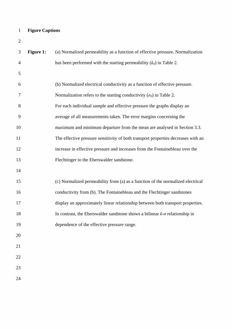
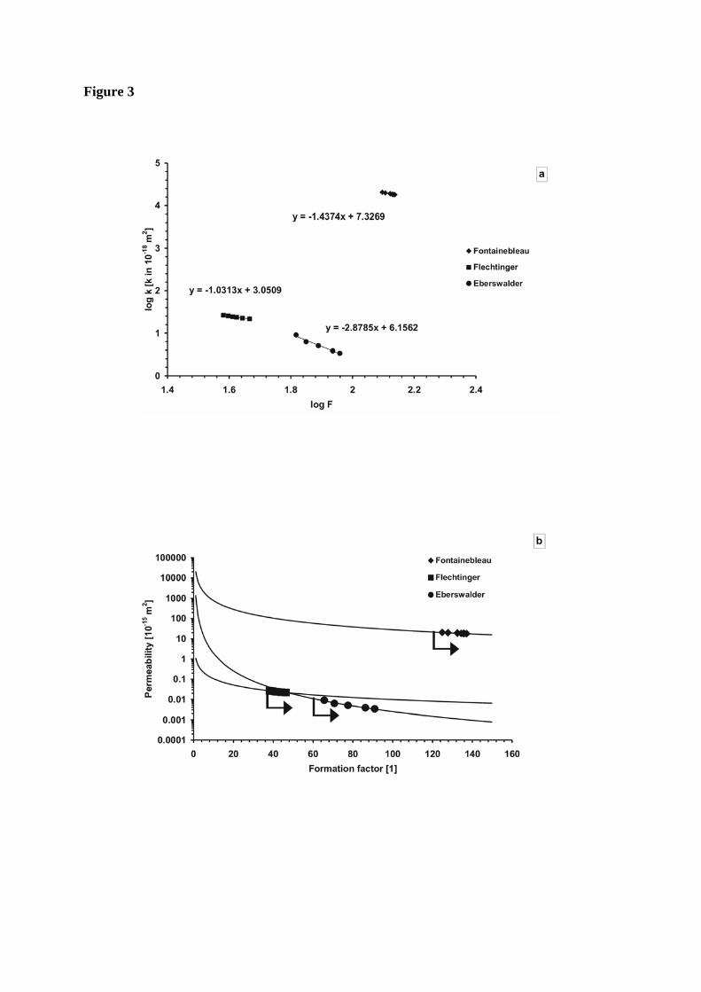
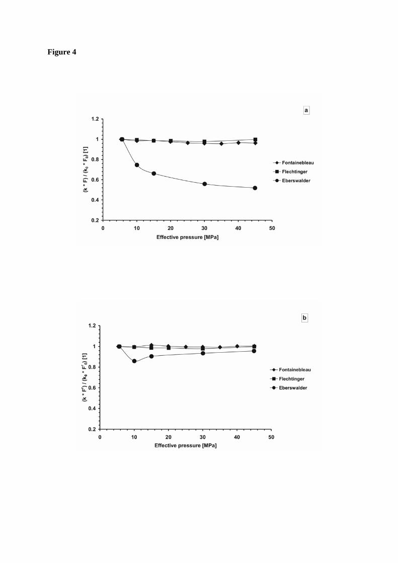
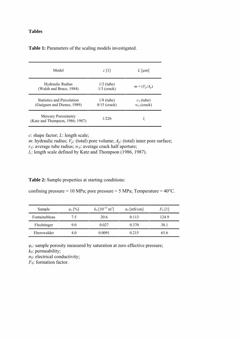
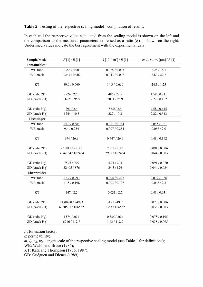
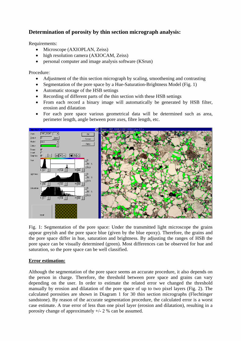
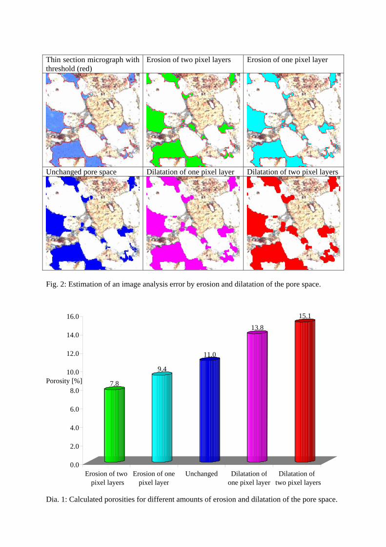The relationship between hydraulic and electrical transport properties in sandstones An experimental evaluation of several scaling models

Harald Milsch1 Guido Bloumlcher1 and Silvio Engelmann1 2

1Deutsches GeoForschungsZentrum Telegrafenberg D-14473 Potsdam Germany milschgfz-potsdamde2Technische Universitaumlt Berlin Institut fuumlr Angewandte Geowissenschaften Ackerstr 76 D-13355 Berlin Germany

Abstract

The purpose of this paper is to investigate the relationship between the parameters that define the hydraulic and electrical transport in porous rock We therefore measured the effective pressure dependence of both permeability (k) and (specific) electrical conductivity (σ) of three different types of sandstones (Fontainebleau Flechtinger and Eberswalder) The experiments were performed in a high pressure and high temperature (HPT) permeameter at a maximum confining- and pore pressure of 50 MPa and 45 MPa respectively and a constant temperature of 40degC 01 molar NaCl-brine was used as the pore fluid We show that for the present rock-fluid combinations surface conductivity can be neglected The experiments were complemented with 2D image analysis and mercury porosimetry to derive the average pore radii the specific inner pore surfaces and the pore radius distributions of the samples The experimental and microstructural results were used to relate both transport properties by means of different length scales and to test the associated scaling models based on (1) the equivalent channel concept (2) statistics and percolation and (3) an interpretation of mercury porosimetry data As the principal result none of these integrated models could adequately reproduce the respective transport property within experimental error margins Furthermore it is emphasized that these models are not applicable for effective pressures other than zero unless the concurrent evolution of the microstructure respectively the length scale can be characterized By comparison it is shown that purely empirical permeability-conductivity relationships can always be adjusted to provide a reasonable description of the coupled k-σdependence on effective pressure However it is implied that the included empirical length parameter is fundamentally different from the ones above as it is a pressure independent constant that contains no true microstructural or physical information

Key Words

permeability electrical conductivity transport properties petrophysics scaling models sandstone

Title Page

1 Introduction1

























26

Main Text

pq η

k (1)27

28

VJ σ (2)29

30









39

FLck

12 (3)40

41























properties64

65

rFLck E

12 (4)66

67










remarks 77

78
















g (Eberswalder) 94









103
































135
























37 nm 159

160

3 Results161

31 Experiments162



























189

































222
























Section 42 246

247













































292

4 Discussion293





























































354








362

)(

3)(

89

1 hmax

lSc

l

hmax

lk (5)363

364

)()(1 e

maxlS

cl

emax

l

F (6)365

366
































397

temaxlcl

thmaxlclh

maxlFk)(

)(2)(32

1

(7)398

and399

)(

)(3)(

89

1e

maxlS

hmaxlS

emaxl

hmaxl

Fk (8)400

401




405

temaxlcl

thmaxlcl

hmaxl

emaxl

emaxlS

hmaxlS

)(

)(

32

89

)(

)(

(9)406

407














419



















factor 438













relationship 451




455

1)])([(3)(2

2 rr

0w

w

0τ

τ (10)456

457




















































509

5 Conclusions510















(model [2])525






















547

548

Acknowledgements549





No BMU 0329951B554

555

556

557

References558










(11) 2529-2540568





3343-3349573



17497-17506576







12267-12278583






Math Geol 21 (1) 1-13589






Phys Rev B 34 (11) 8179-8181595









212 604



6080-6090607













651-662620






Phys Rev B 16 (6) 2597-2612626


19628








doi1010292000JB000057636


(2) 381-389638






Figure Captions 1

2



5









14






20

21

22

23

24




28




32

33




(Eq 4) 37

38




42

43

44

45

46

47

48

49





54








Figures Figure 1

Figure 1 (cont)

Figure 2

Figure 3

Figure 4












Flechtinger 90 0027 0370 381

Eberswalder 40 00091 0215 656




Fontainebleau 137165 217 71 71 023

Flechtinger 50120 144 97 13 14

Eberswalder 2140 123 50 04 114




Flechtinger 0028 370 0028 250

Eberswalder 0013 596 0021 065




WB tube 0366 0003 0065 0003 228 181 WB crack 0244 0002 0043 0002 280 222

KT 800 0660 143 0660 243 123




KT 994 269 0747 269 048 0192



WB tube 177 0297 0004 0297 0039 186 WB crack 118 0198 0003 0198 0048 23

KT 147 25 0031 25 041 0631






φHg [] 71 97 50 264

lc [microm] 1977 250 065 3823 lmax

e [microm] 1153 146 038 2601 S(lmax

e) [1] 090 031 028 057 lmax

h [microm] 1331 199 055 3083 S(lmax

h) [1] 073 017 015 045

kHg [10-15 m2] 693 059 0021 1031 FHg [1] 271 569 1227 98

kexp [10-15 m2] 216 0028 0013 asymp 650












Procedure










78

94

110

138

151

00

20

40

60

80

100

120

140

160

Porosity []









0001

001

01

1

10

001 01 1 10 100


Sam

ple

cond

uctiv

ity [m

Scm

]

01 m NaCl-solution


001

01

1

001 01 1 10 100


Sam

ple

cond

uctiv

ity [m

Scm

]

01 m NaCl-solution


0001

001

01

1

10

001 01 1 10 100


Sam

ple

cond

uctiv

ity [m

Scm

]

01 m NaCl-solution



c = 18






1 Introduction1

























26

Main Text

pq η

k (1)27

28

VJ σ (2)29

30









39

FLck

12 (3)40

41























properties64

65

rFLck E

12 (4)66

67










remarks 77

78
















g (Eberswalder) 94









103
































135
























37 nm 159

160

3 Results161

31 Experiments162



























189

































222
























Section 42 246

247













































292

4 Discussion293





























































354








362

)(

3)(

89

1 hmax

lSc

l

hmax

lk (5)363

364

)()(1 e

maxlS

cl

emax

l

F (6)365

366
































397

temaxlcl

thmaxlclh

maxlFk)(

)(2)(32

1

(7)398

and399

)(

)(3)(

89

1e

maxlS

hmaxlS

emaxl

hmaxl

Fk (8)400

401




405

temaxlcl

thmaxlcl

hmaxl

emaxl

emaxlS

hmaxlS

)(

)(

32

89

)(

)(

(9)406

407














419



















factor 438













relationship 451




455

1)])([(3)(2

2 rr

0w

w

0τ

τ (10)456

457




















































509

5 Conclusions510















(model [2])525






















547

548

Acknowledgements549





No BMU 0329951B554

555

556

557

References558










(11) 2529-2540568





3343-3349573



17497-17506576







12267-12278583






Math Geol 21 (1) 1-13589






Phys Rev B 34 (11) 8179-8181595









212 604



6080-6090607













651-662620






Phys Rev B 16 (6) 2597-2612626


19628








doi1010292000JB000057636


(2) 381-389638






Figure Captions 1

2



5









14






20

21

22

23

24




28




32

33




(Eq 4) 37

38




42

43

44

45

46

47

48

49





54








Figures Figure 1

Figure 1 (cont)

Figure 2

Figure 3

Figure 4












Flechtinger 90 0027 0370 381

Eberswalder 40 00091 0215 656




Fontainebleau 137165 217 71 71 023

Flechtinger 50120 144 97 13 14

Eberswalder 2140 123 50 04 114




Flechtinger 0028 370 0028 250

Eberswalder 0013 596 0021 065




WB tube 0366 0003 0065 0003 228 181 WB crack 0244 0002 0043 0002 280 222

KT 800 0660 143 0660 243 123




KT 994 269 0747 269 048 0192



WB tube 177 0297 0004 0297 0039 186 WB crack 118 0198 0003 0198 0048 23

KT 147 25 0031 25 041 0631






φHg [] 71 97 50 264

lc [microm] 1977 250 065 3823 lmax

e [microm] 1153 146 038 2601 S(lmax

e) [1] 090 031 028 057 lmax

h [microm] 1331 199 055 3083 S(lmax

h) [1] 073 017 015 045

kHg [10-15 m2] 693 059 0021 1031 FHg [1] 271 569 1227 98

kexp [10-15 m2] 216 0028 0013 asymp 650












Procedure










78

94

110

138

151

00

20

40

60

80

100

120

140

160

Porosity []









0001

001

01

1

10

001 01 1 10 100


Sam

ple

cond

uctiv

ity [m

Scm

]

01 m NaCl-solution


001

01

1

001 01 1 10 100


Sam

ple

cond

uctiv

ity [m

Scm

]

01 m NaCl-solution


0001

001

01

1

10

001 01 1 10 100


Sam

ple

cond

uctiv

ity [m

Scm

]

01 m NaCl-solution



c = 18






pq η

k (1)27

28

VJ σ (2)29

30









39

FLck

12 (3)40

41























properties64

65

rFLck E

12 (4)66

67










remarks 77

78
















g (Eberswalder) 94









103
































135
























37 nm 159

160

3 Results161

31 Experiments162



























189

































222
























Section 42 246

247













































292

4 Discussion293





























































354








362

)(

3)(

89

1 hmax

lSc

l

hmax

lk (5)363

364

)()(1 e

maxlS

cl

emax

l

F (6)365

366
































397

temaxlcl

thmaxlclh

maxlFk)(

)(2)(32

1

(7)398

and399

)(

)(3)(

89

1e

maxlS

hmaxlS

emaxl

hmaxl

Fk (8)400

401




405

temaxlcl

thmaxlcl

hmaxl

emaxl

emaxlS

hmaxlS

)(

)(

32

89

)(

)(

(9)406

407














419



















factor 438













relationship 451




455

1)])([(3)(2

2 rr

0w

w

0τ

τ (10)456

457




















































509

5 Conclusions510















(model [2])525






















547

548

Acknowledgements549





No BMU 0329951B554

555

556

557

References558










(11) 2529-2540568





3343-3349573



17497-17506576







12267-12278583






Math Geol 21 (1) 1-13589






Phys Rev B 34 (11) 8179-8181595









212 604



6080-6090607













651-662620






Phys Rev B 16 (6) 2597-2612626


19628








doi1010292000JB000057636


(2) 381-389638






Figure Captions 1

2



5









14






20

21

22

23

24




28




32

33




(Eq 4) 37

38




42

43

44

45

46

47

48

49





54








Figures Figure 1

Figure 1 (cont)

Figure 2

Figure 3

Figure 4












Flechtinger 90 0027 0370 381

Eberswalder 40 00091 0215 656




Fontainebleau 137165 217 71 71 023

Flechtinger 50120 144 97 13 14

Eberswalder 2140 123 50 04 114




Flechtinger 0028 370 0028 250

Eberswalder 0013 596 0021 065




WB tube 0366 0003 0065 0003 228 181 WB crack 0244 0002 0043 0002 280 222

KT 800 0660 143 0660 243 123




KT 994 269 0747 269 048 0192



WB tube 177 0297 0004 0297 0039 186 WB crack 118 0198 0003 0198 0048 23

KT 147 25 0031 25 041 0631






φHg [] 71 97 50 264

lc [microm] 1977 250 065 3823 lmax

e [microm] 1153 146 038 2601 S(lmax

e) [1] 090 031 028 057 lmax

h [microm] 1331 199 055 3083 S(lmax

h) [1] 073 017 015 045

kHg [10-15 m2] 693 059 0021 1031 FHg [1] 271 569 1227 98

kexp [10-15 m2] 216 0028 0013 asymp 650












Procedure










78

94

110

138

151

00

20

40

60

80

100

120

140

160

Porosity []









0001

001

01

1

10

001 01 1 10 100


Sam

ple

cond

uctiv

ity [m

Scm

]

01 m NaCl-solution


001

01

1

001 01 1 10 100


Sam

ple

cond

uctiv

ity [m

Scm

]

01 m NaCl-solution


0001

001

01

1

10

001 01 1 10 100


Sam

ple

cond

uctiv

ity [m

Scm

]

01 m NaCl-solution



c = 18



















properties64

65

rFLck E

12 (4)66

67










remarks 77

78
















g (Eberswalder) 94









103
































135
























37 nm 159

160

3 Results161

31 Experiments162



























189

































222
























Section 42 246

247













































292

4 Discussion293





























































354








362

)(

3)(

89

1 hmax

lSc

l

hmax

lk (5)363

364

)()(1 e

maxlS

cl

emax

l

F (6)365

366
































397

temaxlcl

thmaxlclh

maxlFk)(

)(2)(32

1

(7)398

and399

)(

)(3)(

89

1e

maxlS

hmaxlS

emaxl

hmaxl

Fk (8)400

401




405

temaxlcl

thmaxlcl

hmaxl

emaxl

emaxlS

hmaxlS

)(

)(

32

89

)(

)(

(9)406

407














419



















factor 438













relationship 451




455

1)])([(3)(2

2 rr

0w

w

0τ

τ (10)456

457




















































509

5 Conclusions510















(model [2])525






















547

548

Acknowledgements549





No BMU 0329951B554

555

556

557

References558










(11) 2529-2540568





3343-3349573



17497-17506576







12267-12278583






Math Geol 21 (1) 1-13589






Phys Rev B 34 (11) 8179-8181595









212 604



6080-6090607













651-662620






Phys Rev B 16 (6) 2597-2612626


19628








doi1010292000JB000057636


(2) 381-389638






Figure Captions 1

2



5









14






20

21

22

23

24




28




32

33




(Eq 4) 37

38




42

43

44

45

46

47

48

49





54








Figures Figure 1

Figure 1 (cont)

Figure 2

Figure 3

Figure 4












Flechtinger 90 0027 0370 381

Eberswalder 40 00091 0215 656




Fontainebleau 137165 217 71 71 023

Flechtinger 50120 144 97 13 14

Eberswalder 2140 123 50 04 114




Flechtinger 0028 370 0028 250

Eberswalder 0013 596 0021 065




WB tube 0366 0003 0065 0003 228 181 WB crack 0244 0002 0043 0002 280 222

KT 800 0660 143 0660 243 123




KT 994 269 0747 269 048 0192



WB tube 177 0297 0004 0297 0039 186 WB crack 118 0198 0003 0198 0048 23

KT 147 25 0031 25 041 0631






φHg [] 71 97 50 264

lc [microm] 1977 250 065 3823 lmax

e [microm] 1153 146 038 2601 S(lmax

e) [1] 090 031 028 057 lmax

h [microm] 1331 199 055 3083 S(lmax

h) [1] 073 017 015 045

kHg [10-15 m2] 693 059 0021 1031 FHg [1] 271 569 1227 98

kexp [10-15 m2] 216 0028 0013 asymp 650












Procedure










78

94

110

138

151

00

20

40

60

80

100

120

140

160

Porosity []









0001

001

01

1

10

001 01 1 10 100


Sam

ple

cond

uctiv

ity [m

Scm

]

01 m NaCl-solution


001

01

1

001 01 1 10 100


Sam

ple

cond

uctiv

ity [m

Scm

]

01 m NaCl-solution


0001

001

01

1

10

001 01 1 10 100


Sam

ple

cond

uctiv

ity [m

Scm

]

01 m NaCl-solution



c = 18







remarks 77

78
















g (Eberswalder) 94









103
































135
























37 nm 159

160

3 Results161

31 Experiments162



























189

































222
























Section 42 246

247













































292

4 Discussion293





























































354








362

)(

3)(

89

1 hmax

lSc

l

hmax

lk (5)363

364

)()(1 e

maxlS

cl

emax

l

F (6)365

366
































397

temaxlcl

thmaxlclh

maxlFk)(

)(2)(32

1

(7)398

and399

)(

)(3)(

89

1e

maxlS

hmaxlS

emaxl

hmaxl

Fk (8)400

401




405

temaxlcl

thmaxlcl

hmaxl

emaxl

emaxlS

hmaxlS

)(

)(

32

89

)(

)(

(9)406

407














419



















factor 438













relationship 451




455

1)])([(3)(2

2 rr

0w

w

0τ

τ (10)456

457




















































509

5 Conclusions510















(model [2])525






















547

548

Acknowledgements549





No BMU 0329951B554

555

556

557

References558










(11) 2529-2540568





3343-3349573



17497-17506576







12267-12278583






Math Geol 21 (1) 1-13589






Phys Rev B 34 (11) 8179-8181595









212 604



6080-6090607













651-662620






Phys Rev B 16 (6) 2597-2612626


19628








doi1010292000JB000057636


(2) 381-389638






Figure Captions 1

2



5









14






20

21

22

23

24




28




32

33




(Eq 4) 37

38




42

43

44

45

46

47

48

49





54








Figures Figure 1

Figure 1 (cont)

Figure 2

Figure 3

Figure 4












Flechtinger 90 0027 0370 381

Eberswalder 40 00091 0215 656




Fontainebleau 137165 217 71 71 023

Flechtinger 50120 144 97 13 14

Eberswalder 2140 123 50 04 114




Flechtinger 0028 370 0028 250

Eberswalder 0013 596 0021 065




WB tube 0366 0003 0065 0003 228 181 WB crack 0244 0002 0043 0002 280 222

KT 800 0660 143 0660 243 123




KT 994 269 0747 269 048 0192



WB tube 177 0297 0004 0297 0039 186 WB crack 118 0198 0003 0198 0048 23

KT 147 25 0031 25 041 0631






φHg [] 71 97 50 264

lc [microm] 1977 250 065 3823 lmax

e [microm] 1153 146 038 2601 S(lmax

e) [1] 090 031 028 057 lmax

h [microm] 1331 199 055 3083 S(lmax

h) [1] 073 017 015 045

kHg [10-15 m2] 693 059 0021 1031 FHg [1] 271 569 1227 98

kexp [10-15 m2] 216 0028 0013 asymp 650












Procedure










78

94

110

138

151

00

20

40

60

80

100

120

140

160

Porosity []









0001

001

01

1

10

001 01 1 10 100


Sam

ple

cond

uctiv

ity [m

Scm

]

01 m NaCl-solution


001

01

1

001 01 1 10 100


Sam

ple

cond

uctiv

ity [m

Scm

]

01 m NaCl-solution


0001

001

01

1

10

001 01 1 10 100


Sam

ple

cond

uctiv

ity [m

Scm

]

01 m NaCl-solution



c = 18








103
































135
























37 nm 159

160

3 Results161

31 Experiments162



























189

































222
























Section 42 246

247













































292

4 Discussion293





























































354








362

)(

3)(

89

1 hmax

lSc

l

hmax

lk (5)363

364

)()(1 e

maxlS

cl

emax

l

F (6)365

366
































397

temaxlcl

thmaxlclh

maxlFk)(

)(2)(32

1

(7)398

and399

)(

)(3)(

89

1e

maxlS

hmaxlS

emaxl

hmaxl

Fk (8)400

401




405

temaxlcl

thmaxlcl

hmaxl

emaxl

emaxlS

hmaxlS

)(

)(

32

89

)(

)(

(9)406

407














419



















factor 438













relationship 451




455

1)])([(3)(2

2 rr

0w

w

0τ

τ (10)456

457




















































509

5 Conclusions510















(model [2])525






















547

548

Acknowledgements549





No BMU 0329951B554

555

556

557

References558










(11) 2529-2540568





3343-3349573



17497-17506576







12267-12278583






Math Geol 21 (1) 1-13589






Phys Rev B 34 (11) 8179-8181595









212 604



6080-6090607













651-662620






Phys Rev B 16 (6) 2597-2612626


19628








doi1010292000JB000057636


(2) 381-389638






Figure Captions 1

2



5









14






20

21

22

23

24




28




32

33




(Eq 4) 37

38




42

43

44

45

46

47

48

49





54








Figures Figure 1

Figure 1 (cont)

Figure 2

Figure 3

Figure 4












Flechtinger 90 0027 0370 381

Eberswalder 40 00091 0215 656




Fontainebleau 137165 217 71 71 023

Flechtinger 50120 144 97 13 14

Eberswalder 2140 123 50 04 114




Flechtinger 0028 370 0028 250

Eberswalder 0013 596 0021 065




WB tube 0366 0003 0065 0003 228 181 WB crack 0244 0002 0043 0002 280 222

KT 800 0660 143 0660 243 123




KT 994 269 0747 269 048 0192



WB tube 177 0297 0004 0297 0039 186 WB crack 118 0198 0003 0198 0048 23

KT 147 25 0031 25 041 0631






φHg [] 71 97 50 264

lc [microm] 1977 250 065 3823 lmax

e [microm] 1153 146 038 2601 S(lmax

e) [1] 090 031 028 057 lmax

h [microm] 1331 199 055 3083 S(lmax

h) [1] 073 017 015 045

kHg [10-15 m2] 693 059 0021 1031 FHg [1] 271 569 1227 98

kexp [10-15 m2] 216 0028 0013 asymp 650












Procedure










78

94

110

138

151

00

20

40

60

80

100

120

140

160

Porosity []









0001

001

01

1

10

001 01 1 10 100


Sam

ple

cond

uctiv

ity [m

Scm

]

01 m NaCl-solution


001

01

1

001 01 1 10 100


Sam

ple

cond

uctiv

ity [m

Scm

]

01 m NaCl-solution


0001

001

01

1

10

001 01 1 10 100


Sam

ple

cond

uctiv

ity [m

Scm

]

01 m NaCl-solution



c = 18














135
























37 nm 159

160

3 Results161

31 Experiments162



























189

































222
























Section 42 246

247













































292

4 Discussion293





























































354








362

)(

3)(

89

1 hmax

lSc

l

hmax

lk (5)363

364

)()(1 e

maxlS

cl

emax

l

F (6)365

366
































397

temaxlcl

thmaxlclh

maxlFk)(

)(2)(32

1

(7)398

and399

)(

)(3)(

89

1e

maxlS

hmaxlS

emaxl

hmaxl

Fk (8)400

401




405

temaxlcl

thmaxlcl

hmaxl

emaxl

emaxlS

hmaxlS

)(

)(

32

89

)(

)(

(9)406

407














419



















factor 438













relationship 451




455

1)])([(3)(2

2 rr

0w

w

0τ

τ (10)456

457




















































509

5 Conclusions510















(model [2])525






















547

548

Acknowledgements549





No BMU 0329951B554

555

556

557

References558










(11) 2529-2540568





3343-3349573



17497-17506576







12267-12278583






Math Geol 21 (1) 1-13589






Phys Rev B 34 (11) 8179-8181595









212 604



6080-6090607













651-662620






Phys Rev B 16 (6) 2597-2612626


19628








doi1010292000JB000057636


(2) 381-389638






Figure Captions 1

2



5









14






20

21

22

23

24




28




32

33




(Eq 4) 37

38




42

43

44

45

46

47

48

49





54








Figures Figure 1

Figure 1 (cont)

Figure 2

Figure 3

Figure 4












Flechtinger 90 0027 0370 381

Eberswalder 40 00091 0215 656




Fontainebleau 137165 217 71 71 023

Flechtinger 50120 144 97 13 14

Eberswalder 2140 123 50 04 114




Flechtinger 0028 370 0028 250

Eberswalder 0013 596 0021 065




WB tube 0366 0003 0065 0003 228 181 WB crack 0244 0002 0043 0002 280 222

KT 800 0660 143 0660 243 123




KT 994 269 0747 269 048 0192



WB tube 177 0297 0004 0297 0039 186 WB crack 118 0198 0003 0198 0048 23

KT 147 25 0031 25 041 0631






φHg [] 71 97 50 264

lc [microm] 1977 250 065 3823 lmax

e [microm] 1153 146 038 2601 S(lmax

e) [1] 090 031 028 057 lmax

h [microm] 1331 199 055 3083 S(lmax

h) [1] 073 017 015 045

kHg [10-15 m2] 693 059 0021 1031 FHg [1] 271 569 1227 98

kexp [10-15 m2] 216 0028 0013 asymp 650












Procedure










78

94

110

138

151

00

20

40

60

80

100

120

140

160

Porosity []









0001

001

01

1

10

001 01 1 10 100


Sam

ple

cond

uctiv

ity [m

Scm

]

01 m NaCl-solution


001

01

1

001 01 1 10 100


Sam

ple

cond

uctiv

ity [m

Scm

]

01 m NaCl-solution


0001

001

01

1

10

001 01 1 10 100


Sam

ple

cond

uctiv

ity [m

Scm

]

01 m NaCl-solution



c = 18












37 nm 159

160

3 Results161

31 Experiments162



























189

































222
























Section 42 246

247













































292

4 Discussion293





























































354








362

)(

3)(

89

1 hmax

lSc

l

hmax

lk (5)363

364

)()(1 e

maxlS

cl

emax

l

F (6)365

366
































397

temaxlcl

thmaxlclh

maxlFk)(

)(2)(32

1

(7)398

and399

)(

)(3)(

89

1e

maxlS

hmaxlS

emaxl

hmaxl

Fk (8)400

401




405

temaxlcl

thmaxlcl

hmaxl

emaxl

emaxlS

hmaxlS

)(

)(

32

89

)(

)(

(9)406

407














419



















factor 438













relationship 451




455

1)])([(3)(2

2 rr

0w

w

0τ

τ (10)456

457




















































509

5 Conclusions510















(model [2])525






















547

548

Acknowledgements549





No BMU 0329951B554

555

556

557

References558










(11) 2529-2540568





3343-3349573



17497-17506576







12267-12278583






Math Geol 21 (1) 1-13589






Phys Rev B 34 (11) 8179-8181595









212 604



6080-6090607













651-662620






Phys Rev B 16 (6) 2597-2612626


19628








doi1010292000JB000057636


(2) 381-389638






Figure Captions 1

2



5









14






20

21

22

23

24




28




32

33




(Eq 4) 37

38




42

43

44

45

46

47

48

49





54








Figures Figure 1

Figure 1 (cont)

Figure 2

Figure 3

Figure 4












Flechtinger 90 0027 0370 381

Eberswalder 40 00091 0215 656




Fontainebleau 137165 217 71 71 023

Flechtinger 50120 144 97 13 14

Eberswalder 2140 123 50 04 114




Flechtinger 0028 370 0028 250

Eberswalder 0013 596 0021 065




WB tube 0366 0003 0065 0003 228 181 WB crack 0244 0002 0043 0002 280 222

KT 800 0660 143 0660 243 123




KT 994 269 0747 269 048 0192



WB tube 177 0297 0004 0297 0039 186 WB crack 118 0198 0003 0198 0048 23

KT 147 25 0031 25 041 0631






φHg [] 71 97 50 264

lc [microm] 1977 250 065 3823 lmax

e [microm] 1153 146 038 2601 S(lmax

e) [1] 090 031 028 057 lmax

h [microm] 1331 199 055 3083 S(lmax

h) [1] 073 017 015 045

kHg [10-15 m2] 693 059 0021 1031 FHg [1] 271 569 1227 98

kexp [10-15 m2] 216 0028 0013 asymp 650












Procedure










78

94

110

138

151

00

20

40

60

80

100

120

140

160

Porosity []









0001

001

01

1

10

001 01 1 10 100


Sam

ple

cond

uctiv

ity [m

Scm

]

01 m NaCl-solution


001

01

1

001 01 1 10 100


Sam

ple

cond

uctiv

ity [m

Scm

]

01 m NaCl-solution


0001

001

01

1

10

001 01 1 10 100


Sam

ple

cond

uctiv

ity [m

Scm

]

01 m NaCl-solution



c = 18
















189

































222
























Section 42 246

247













































292

4 Discussion293





























































354








362

)(

3)(

89

1 hmax

lSc

l

hmax

lk (5)363

364

)()(1 e

maxlS

cl

emax

l

F (6)365

366
































397

temaxlcl

thmaxlclh

maxlFk)(

)(2)(32

1

(7)398

and399

)(

)(3)(

89

1e

maxlS

hmaxlS

emaxl

hmaxl

Fk (8)400

401




405

temaxlcl

thmaxlcl

hmaxl

emaxl

emaxlS

hmaxlS

)(

)(

32

89

)(

)(

(9)406

407














419



















factor 438













relationship 451




455

1)])([(3)(2

2 rr

0w

w

0τ

τ (10)456

457




















































509

5 Conclusions510















(model [2])525






















547

548

Acknowledgements549





No BMU 0329951B554

555

556

557

References558










(11) 2529-2540568





3343-3349573



17497-17506576







12267-12278583






Math Geol 21 (1) 1-13589






Phys Rev B 34 (11) 8179-8181595









212 604



6080-6090607













651-662620






Phys Rev B 16 (6) 2597-2612626


19628








doi1010292000JB000057636


(2) 381-389638






Figure Captions 1

2



5









14






20

21

22

23

24




28




32

33




(Eq 4) 37

38




42

43

44

45

46

47

48

49





54








Figures Figure 1

Figure 1 (cont)

Figure 2

Figure 3

Figure 4












Flechtinger 90 0027 0370 381

Eberswalder 40 00091 0215 656




Fontainebleau 137165 217 71 71 023

Flechtinger 50120 144 97 13 14

Eberswalder 2140 123 50 04 114




Flechtinger 0028 370 0028 250

Eberswalder 0013 596 0021 065




WB tube 0366 0003 0065 0003 228 181 WB crack 0244 0002 0043 0002 280 222

KT 800 0660 143 0660 243 123




KT 994 269 0747 269 048 0192



WB tube 177 0297 0004 0297 0039 186 WB crack 118 0198 0003 0198 0048 23

KT 147 25 0031 25 041 0631






φHg [] 71 97 50 264

lc [microm] 1977 250 065 3823 lmax

e [microm] 1153 146 038 2601 S(lmax

e) [1] 090 031 028 057 lmax

h [microm] 1331 199 055 3083 S(lmax

h) [1] 073 017 015 045

kHg [10-15 m2] 693 059 0021 1031 FHg [1] 271 569 1227 98

kexp [10-15 m2] 216 0028 0013 asymp 650












Procedure










78

94

110

138

151

00

20

40

60

80

100

120

140

160

Porosity []









0001

001

01

1

10

001 01 1 10 100


Sam

ple

cond

uctiv

ity [m

Scm

]

01 m NaCl-solution


001

01

1

001 01 1 10 100


Sam

ple

cond

uctiv

ity [m

Scm

]

01 m NaCl-solution


0001

001

01

1

10

001 01 1 10 100


Sam

ple

cond

uctiv

ity [m

Scm

]

01 m NaCl-solution



c = 18























222
























Section 42 246

247













































292

4 Discussion293





























































354








362

)(

3)(

89

1 hmax

lSc

l

hmax

lk (5)363

364

)()(1 e

maxlS

cl

emax

l

F (6)365

366
































397

temaxlcl

thmaxlclh

maxlFk)(

)(2)(32

1

(7)398

and399

)(

)(3)(

89

1e

maxlS

hmaxlS

emaxl

hmaxl

Fk (8)400

401




405

temaxlcl

thmaxlcl

hmaxl

emaxl

emaxlS

hmaxlS

)(

)(

32

89

)(

)(

(9)406

407














419



















factor 438













relationship 451




455

1)])([(3)(2

2 rr

0w

w

0τ

τ (10)456

457




















































509

5 Conclusions510















(model [2])525






















547

548

Acknowledgements549





No BMU 0329951B554

555

556

557

References558










(11) 2529-2540568





3343-3349573



17497-17506576







12267-12278583






Math Geol 21 (1) 1-13589






Phys Rev B 34 (11) 8179-8181595









212 604



6080-6090607













651-662620






Phys Rev B 16 (6) 2597-2612626


19628








doi1010292000JB000057636


(2) 381-389638






Figure Captions 1

2



5









14






20

21

22

23

24




28




32

33




(Eq 4) 37

38




42

43

44

45

46

47

48

49





54








Figures Figure 1

Figure 1 (cont)

Figure 2

Figure 3

Figure 4












Flechtinger 90 0027 0370 381

Eberswalder 40 00091 0215 656




Fontainebleau 137165 217 71 71 023

Flechtinger 50120 144 97 13 14

Eberswalder 2140 123 50 04 114




Flechtinger 0028 370 0028 250

Eberswalder 0013 596 0021 065




WB tube 0366 0003 0065 0003 228 181 WB crack 0244 0002 0043 0002 280 222

KT 800 0660 143 0660 243 123




KT 994 269 0747 269 048 0192



WB tube 177 0297 0004 0297 0039 186 WB crack 118 0198 0003 0198 0048 23

KT 147 25 0031 25 041 0631






φHg [] 71 97 50 264

lc [microm] 1977 250 065 3823 lmax

e [microm] 1153 146 038 2601 S(lmax

e) [1] 090 031 028 057 lmax

h [microm] 1331 199 055 3083 S(lmax

h) [1] 073 017 015 045

kHg [10-15 m2] 693 059 0021 1031 FHg [1] 271 569 1227 98

kexp [10-15 m2] 216 0028 0013 asymp 650












Procedure










78

94

110

138

151

00

20

40

60

80

100

120

140

160

Porosity []









0001

001

01

1

10

001 01 1 10 100


Sam

ple

cond

uctiv

ity [m

Scm

]

01 m NaCl-solution


001

01

1

001 01 1 10 100


Sam

ple

cond

uctiv

ity [m

Scm

]

01 m NaCl-solution


0001

001

01

1

10

001 01 1 10 100


Sam

ple

cond

uctiv

ity [m

Scm

]

01 m NaCl-solution



c = 18





















Section 42 246

247













































292

4 Discussion293





























































354








362

)(

3)(

89

1 hmax

lSc

l

hmax

lk (5)363

364

)()(1 e

maxlS

cl

emax

l

F (6)365

366
































397

temaxlcl

thmaxlclh

maxlFk)(

)(2)(32

1

(7)398

and399

)(

)(3)(

89

1e

maxlS

hmaxlS

emaxl

hmaxl

Fk (8)400

401




405

temaxlcl

thmaxlcl

hmaxl

emaxl

emaxlS

hmaxlS

)(

)(

32

89

)(

)(

(9)406

407














419



















factor 438













relationship 451




455

1)])([(3)(2

2 rr

0w

w

0τ

τ (10)456

457




















































509

5 Conclusions510















(model [2])525






















547

548

Acknowledgements549





No BMU 0329951B554

555

556

557

References558










(11) 2529-2540568





3343-3349573



17497-17506576







12267-12278583






Math Geol 21 (1) 1-13589






Phys Rev B 34 (11) 8179-8181595









212 604



6080-6090607













651-662620






Phys Rev B 16 (6) 2597-2612626


19628








doi1010292000JB000057636


(2) 381-389638






Figure Captions 1

2



5









14






20

21

22

23

24




28




32

33




(Eq 4) 37

38




42

43

44

45

46

47

48

49





54








Figures Figure 1

Figure 1 (cont)

Figure 2

Figure 3

Figure 4












Flechtinger 90 0027 0370 381

Eberswalder 40 00091 0215 656




Fontainebleau 137165 217 71 71 023

Flechtinger 50120 144 97 13 14

Eberswalder 2140 123 50 04 114




Flechtinger 0028 370 0028 250

Eberswalder 0013 596 0021 065




WB tube 0366 0003 0065 0003 228 181 WB crack 0244 0002 0043 0002 280 222

KT 800 0660 143 0660 243 123




KT 994 269 0747 269 048 0192



WB tube 177 0297 0004 0297 0039 186 WB crack 118 0198 0003 0198 0048 23

KT 147 25 0031 25 041 0631






φHg [] 71 97 50 264

lc [microm] 1977 250 065 3823 lmax

e [microm] 1153 146 038 2601 S(lmax

e) [1] 090 031 028 057 lmax

h [microm] 1331 199 055 3083 S(lmax

h) [1] 073 017 015 045

kHg [10-15 m2] 693 059 0021 1031 FHg [1] 271 569 1227 98

kexp [10-15 m2] 216 0028 0013 asymp 650












Procedure










78

94

110

138

151

00

20

40

60

80

100

120

140

160

Porosity []









0001

001

01

1

10

001 01 1 10 100


Sam

ple

cond

uctiv

ity [m

Scm

]

01 m NaCl-solution


001

01

1

001 01 1 10 100


Sam

ple

cond

uctiv

ity [m

Scm

]

01 m NaCl-solution


0001

001

01

1

10

001 01 1 10 100


Sam

ple

cond

uctiv

ity [m

Scm

]

01 m NaCl-solution



c = 18









































292

4 Discussion293





























































354








362

)(

3)(

89

1 hmax

lSc

l

hmax

lk (5)363

364

)()(1 e

maxlS

cl

emax

l

F (6)365

366
































397

temaxlcl

thmaxlclh

maxlFk)(

)(2)(32

1

(7)398

and399

)(

)(3)(

89

1e

maxlS

hmaxlS

emaxl

hmaxl

Fk (8)400

401




405

temaxlcl

thmaxlcl

hmaxl

emaxl

emaxlS

hmaxlS

)(

)(

32

89

)(

)(

(9)406

407














419



















factor 438













relationship 451




455

1)])([(3)(2

2 rr

0w

w

0τ

τ (10)456

457




















































509

5 Conclusions510















(model [2])525






















547

548

Acknowledgements549





No BMU 0329951B554

555

556

557

References558










(11) 2529-2540568





3343-3349573



17497-17506576







12267-12278583






Math Geol 21 (1) 1-13589






Phys Rev B 34 (11) 8179-8181595









212 604



6080-6090607













651-662620






Phys Rev B 16 (6) 2597-2612626


19628








doi1010292000JB000057636


(2) 381-389638






Figure Captions 1

2



5









14






20

21

22

23

24




28




32

33




(Eq 4) 37

38




42

43

44

45

46

47

48

49





54








Figures Figure 1

Figure 1 (cont)

Figure 2

Figure 3

Figure 4












Flechtinger 90 0027 0370 381

Eberswalder 40 00091 0215 656




Fontainebleau 137165 217 71 71 023

Flechtinger 50120 144 97 13 14

Eberswalder 2140 123 50 04 114




Flechtinger 0028 370 0028 250

Eberswalder 0013 596 0021 065




WB tube 0366 0003 0065 0003 228 181 WB crack 0244 0002 0043 0002 280 222

KT 800 0660 143 0660 243 123




KT 994 269 0747 269 048 0192



WB tube 177 0297 0004 0297 0039 186 WB crack 118 0198 0003 0198 0048 23

KT 147 25 0031 25 041 0631






φHg [] 71 97 50 264

lc [microm] 1977 250 065 3823 lmax

e [microm] 1153 146 038 2601 S(lmax

e) [1] 090 031 028 057 lmax

h [microm] 1331 199 055 3083 S(lmax

h) [1] 073 017 015 045

kHg [10-15 m2] 693 059 0021 1031 FHg [1] 271 569 1227 98

kexp [10-15 m2] 216 0028 0013 asymp 650












Procedure










78

94

110

138

151

00

20

40

60

80

100

120

140

160

Porosity []









0001

001

01

1

10

001 01 1 10 100


Sam

ple

cond

uctiv

ity [m

Scm

]

01 m NaCl-solution


001

01

1

001 01 1 10 100


Sam

ple

cond

uctiv

ity [m

Scm

]

01 m NaCl-solution


0001

001

01

1

10

001 01 1 10 100


Sam

ple

cond

uctiv

ity [m

Scm

]

01 m NaCl-solution



c = 18




















































354








362

)(

3)(

89

1 hmax

lSc

l

hmax

lk (5)363

364

)()(1 e

maxlS

cl

emax

l

F (6)365

366
































397

temaxlcl

thmaxlclh

maxlFk)(

)(2)(32

1

(7)398

and399

)(

)(3)(

89

1e

maxlS

hmaxlS

emaxl

hmaxl

Fk (8)400

401




405

temaxlcl

thmaxlcl

hmaxl

emaxl

emaxlS

hmaxlS

)(

)(

32

89

)(

)(

(9)406

407














419



















factor 438













relationship 451




455

1)])([(3)(2

2 rr

0w

w

0τ

τ (10)456

457




















































509

5 Conclusions510















(model [2])525






















547

548

Acknowledgements549





No BMU 0329951B554

555

556

557

References558










(11) 2529-2540568





3343-3349573



17497-17506576







12267-12278583






Math Geol 21 (1) 1-13589






Phys Rev B 34 (11) 8179-8181595









212 604



6080-6090607













651-662620






Phys Rev B 16 (6) 2597-2612626


19628








doi1010292000JB000057636


(2) 381-389638






Figure Captions 1

2



5









14






20

21

22

23

24




28




32

33




(Eq 4) 37

38




42

43

44

45

46

47

48

49





54








Figures Figure 1

Figure 1 (cont)

Figure 2

Figure 3

Figure 4












Flechtinger 90 0027 0370 381

Eberswalder 40 00091 0215 656




Fontainebleau 137165 217 71 71 023

Flechtinger 50120 144 97 13 14

Eberswalder 2140 123 50 04 114




Flechtinger 0028 370 0028 250

Eberswalder 0013 596 0021 065




WB tube 0366 0003 0065 0003 228 181 WB crack 0244 0002 0043 0002 280 222

KT 800 0660 143 0660 243 123




KT 994 269 0747 269 048 0192



WB tube 177 0297 0004 0297 0039 186 WB crack 118 0198 0003 0198 0048 23

KT 147 25 0031 25 041 0631






φHg [] 71 97 50 264

lc [microm] 1977 250 065 3823 lmax

e [microm] 1153 146 038 2601 S(lmax

e) [1] 090 031 028 057 lmax

h [microm] 1331 199 055 3083 S(lmax

h) [1] 073 017 015 045

kHg [10-15 m2] 693 059 0021 1031 FHg [1] 271 569 1227 98

kexp [10-15 m2] 216 0028 0013 asymp 650












Procedure










78

94

110

138

151

00

20

40

60

80

100

120

140

160

Porosity []









0001

001

01

1

10

001 01 1 10 100


Sam

ple

cond

uctiv

ity [m

Scm

]

01 m NaCl-solution


001

01

1

001 01 1 10 100


Sam

ple

cond

uctiv

ity [m

Scm

]

01 m NaCl-solution


0001

001

01

1

10

001 01 1 10 100


Sam

ple

cond

uctiv

ity [m

Scm

]

01 m NaCl-solution



c = 18








362

)(

3)(

89

1 hmax

lSc

l

hmax

lk (5)363

364

)()(1 e

maxlS

cl

emax

l

F (6)365

366
































397

temaxlcl

thmaxlclh

maxlFk)(

)(2)(32

1

(7)398

and399

)(

)(3)(

89

1e

maxlS

hmaxlS

emaxl

hmaxl

Fk (8)400

401




405

temaxlcl

thmaxlcl

hmaxl

emaxl

emaxlS

hmaxlS

)(

)(

32

89

)(

)(

(9)406

407














419



















factor 438













relationship 451




455

1)])([(3)(2

2 rr

0w

w

0τ

τ (10)456

457




















































509

5 Conclusions510















(model [2])525






















547

548

Acknowledgements549





No BMU 0329951B554

555

556

557

References558










(11) 2529-2540568





3343-3349573



17497-17506576







12267-12278583






Math Geol 21 (1) 1-13589






Phys Rev B 34 (11) 8179-8181595









212 604



6080-6090607













651-662620






Phys Rev B 16 (6) 2597-2612626


19628








doi1010292000JB000057636


(2) 381-389638






Figure Captions 1

2



5









14






20

21

22

23

24




28




32

33




(Eq 4) 37

38




42

43

44

45

46

47

48

49





54








Figures Figure 1

Figure 1 (cont)

Figure 2

Figure 3

Figure 4












Flechtinger 90 0027 0370 381

Eberswalder 40 00091 0215 656




Fontainebleau 137165 217 71 71 023

Flechtinger 50120 144 97 13 14

Eberswalder 2140 123 50 04 114




Flechtinger 0028 370 0028 250

Eberswalder 0013 596 0021 065




WB tube 0366 0003 0065 0003 228 181 WB crack 0244 0002 0043 0002 280 222

KT 800 0660 143 0660 243 123




KT 994 269 0747 269 048 0192



WB tube 177 0297 0004 0297 0039 186 WB crack 118 0198 0003 0198 0048 23

KT 147 25 0031 25 041 0631






φHg [] 71 97 50 264

lc [microm] 1977 250 065 3823 lmax

e [microm] 1153 146 038 2601 S(lmax

e) [1] 090 031 028 057 lmax

h [microm] 1331 199 055 3083 S(lmax

h) [1] 073 017 015 045

kHg [10-15 m2] 693 059 0021 1031 FHg [1] 271 569 1227 98

kexp [10-15 m2] 216 0028 0013 asymp 650












Procedure










78

94

110

138

151

00

20

40

60

80

100

120

140

160

Porosity []









0001

001

01

1

10

001 01 1 10 100


Sam

ple

cond

uctiv

ity [m

Scm

]

01 m NaCl-solution


001

01

1

001 01 1 10 100


Sam

ple

cond

uctiv

ity [m

Scm

]

01 m NaCl-solution


0001

001

01

1

10

001 01 1 10 100


Sam

ple

cond

uctiv

ity [m

Scm

]

01 m NaCl-solution



c = 18




















397

temaxlcl

thmaxlclh

maxlFk)(

)(2)(32

1

(7)398

and399

)(

)(3)(

89

1e

maxlS

hmaxlS

emaxl

hmaxl

Fk (8)400

401




405

temaxlcl

thmaxlcl

hmaxl

emaxl

emaxlS

hmaxlS

)(

)(

32

89

)(

)(

(9)406

407














419



















factor 438













relationship 451




455

1)])([(3)(2

2 rr

0w

w

0τ

τ (10)456

457




















































509

5 Conclusions510















(model [2])525






















547

548

Acknowledgements549





No BMU 0329951B554

555

556

557

References558










(11) 2529-2540568





3343-3349573



17497-17506576







12267-12278583






Math Geol 21 (1) 1-13589






Phys Rev B 34 (11) 8179-8181595









212 604



6080-6090607













651-662620






Phys Rev B 16 (6) 2597-2612626


19628








doi1010292000JB000057636


(2) 381-389638






Figure Captions 1

2



5









14






20

21

22

23

24




28




32

33




(Eq 4) 37

38




42

43

44

45

46

47

48

49





54








Figures Figure 1

Figure 1 (cont)

Figure 2

Figure 3

Figure 4












Flechtinger 90 0027 0370 381

Eberswalder 40 00091 0215 656




Fontainebleau 137165 217 71 71 023

Flechtinger 50120 144 97 13 14

Eberswalder 2140 123 50 04 114




Flechtinger 0028 370 0028 250

Eberswalder 0013 596 0021 065




WB tube 0366 0003 0065 0003 228 181 WB crack 0244 0002 0043 0002 280 222

KT 800 0660 143 0660 243 123




KT 994 269 0747 269 048 0192



WB tube 177 0297 0004 0297 0039 186 WB crack 118 0198 0003 0198 0048 23

KT 147 25 0031 25 041 0631






φHg [] 71 97 50 264

lc [microm] 1977 250 065 3823 lmax

e [microm] 1153 146 038 2601 S(lmax

e) [1] 090 031 028 057 lmax

h [microm] 1331 199 055 3083 S(lmax

h) [1] 073 017 015 045

kHg [10-15 m2] 693 059 0021 1031 FHg [1] 271 569 1227 98

kexp [10-15 m2] 216 0028 0013 asymp 650












Procedure










78

94

110

138

151

00

20

40

60

80

100

120

140

160

Porosity []









0001

001

01

1

10

001 01 1 10 100


Sam

ple

cond

uctiv

ity [m

Scm

]

01 m NaCl-solution


001

01

1

001 01 1 10 100


Sam

ple

cond

uctiv

ity [m

Scm

]

01 m NaCl-solution


0001

001

01

1

10

001 01 1 10 100


Sam

ple

cond

uctiv

ity [m

Scm

]

01 m NaCl-solution



c = 18






temaxlcl

thmaxlcl

hmaxl

emaxl

emaxlS

hmaxlS

)(

)(

32

89

)(

)(

(9)406

407














419



















factor 438













relationship 451




455

1)])([(3)(2

2 rr

0w

w

0τ

τ (10)456

457




















































509

5 Conclusions510















(model [2])525






















547

548

Acknowledgements549





No BMU 0329951B554

555

556

557

References558










(11) 2529-2540568





3343-3349573



17497-17506576







12267-12278583






Math Geol 21 (1) 1-13589






Phys Rev B 34 (11) 8179-8181595









212 604



6080-6090607













651-662620






Phys Rev B 16 (6) 2597-2612626


19628








doi1010292000JB000057636


(2) 381-389638






Figure Captions 1

2



5









14






20

21

22

23

24




28




32

33




(Eq 4) 37

38




42

43

44

45

46

47

48

49





54








Figures Figure 1

Figure 1 (cont)

Figure 2

Figure 3

Figure 4












Flechtinger 90 0027 0370 381

Eberswalder 40 00091 0215 656




Fontainebleau 137165 217 71 71 023

Flechtinger 50120 144 97 13 14

Eberswalder 2140 123 50 04 114




Flechtinger 0028 370 0028 250

Eberswalder 0013 596 0021 065




WB tube 0366 0003 0065 0003 228 181 WB crack 0244 0002 0043 0002 280 222

KT 800 0660 143 0660 243 123




KT 994 269 0747 269 048 0192



WB tube 177 0297 0004 0297 0039 186 WB crack 118 0198 0003 0198 0048 23

KT 147 25 0031 25 041 0631






φHg [] 71 97 50 264

lc [microm] 1977 250 065 3823 lmax

e [microm] 1153 146 038 2601 S(lmax

e) [1] 090 031 028 057 lmax

h [microm] 1331 199 055 3083 S(lmax

h) [1] 073 017 015 045

kHg [10-15 m2] 693 059 0021 1031 FHg [1] 271 569 1227 98

kexp [10-15 m2] 216 0028 0013 asymp 650












Procedure










78

94

110

138

151

00

20

40

60

80

100

120

140

160

Porosity []









0001

001

01

1

10

001 01 1 10 100


Sam

ple

cond

uctiv

ity [m

Scm

]

01 m NaCl-solution


001

01

1

001 01 1 10 100


Sam

ple

cond

uctiv

ity [m

Scm

]

01 m NaCl-solution


0001

001

01

1

10

001 01 1 10 100


Sam

ple

cond

uctiv

ity [m

Scm

]

01 m NaCl-solution



c = 18














factor 438













relationship 451




455

1)])([(3)(2

2 rr

0w

w

0τ

τ (10)456

457




















































509

5 Conclusions510















(model [2])525






















547

548

Acknowledgements549





No BMU 0329951B554

555

556

557

References558










(11) 2529-2540568





3343-3349573



17497-17506576







12267-12278583






Math Geol 21 (1) 1-13589






Phys Rev B 34 (11) 8179-8181595









212 604



6080-6090607













651-662620






Phys Rev B 16 (6) 2597-2612626


19628








doi1010292000JB000057636


(2) 381-389638






Figure Captions 1

2



5









14






20

21

22

23

24




28




32

33




(Eq 4) 37

38




42

43

44

45

46

47

48

49





54








Figures Figure 1

Figure 1 (cont)

Figure 2

Figure 3

Figure 4












Flechtinger 90 0027 0370 381

Eberswalder 40 00091 0215 656




Fontainebleau 137165 217 71 71 023

Flechtinger 50120 144 97 13 14

Eberswalder 2140 123 50 04 114




Flechtinger 0028 370 0028 250

Eberswalder 0013 596 0021 065




WB tube 0366 0003 0065 0003 228 181 WB crack 0244 0002 0043 0002 280 222

KT 800 0660 143 0660 243 123




KT 994 269 0747 269 048 0192



WB tube 177 0297 0004 0297 0039 186 WB crack 118 0198 0003 0198 0048 23

KT 147 25 0031 25 041 0631






φHg [] 71 97 50 264

lc [microm] 1977 250 065 3823 lmax

e [microm] 1153 146 038 2601 S(lmax

e) [1] 090 031 028 057 lmax

h [microm] 1331 199 055 3083 S(lmax

h) [1] 073 017 015 045

kHg [10-15 m2] 693 059 0021 1031 FHg [1] 271 569 1227 98

kexp [10-15 m2] 216 0028 0013 asymp 650












Procedure










78

94

110

138

151

00

20

40

60

80

100

120

140

160

Porosity []









0001

001

01

1

10

001 01 1 10 100


Sam

ple

cond

uctiv

ity [m

Scm

]

01 m NaCl-solution


001

01

1

001 01 1 10 100


Sam

ple

cond

uctiv

ity [m

Scm

]

01 m NaCl-solution


0001

001

01

1

10

001 01 1 10 100


Sam

ple

cond

uctiv

ity [m

Scm

]

01 m NaCl-solution



c = 18






1)])([(3)(2

2 rr

0w

w

0τ

τ (10)456

457




















































509

5 Conclusions510















(model [2])525






















547

548

Acknowledgements549





No BMU 0329951B554

555

556

557

References558










(11) 2529-2540568





3343-3349573



17497-17506576







12267-12278583






Math Geol 21 (1) 1-13589






Phys Rev B 34 (11) 8179-8181595









212 604



6080-6090607













651-662620






Phys Rev B 16 (6) 2597-2612626


19628








doi1010292000JB000057636


(2) 381-389638






Figure Captions 1

2



5









14






20

21

22

23

24




28




32

33




(Eq 4) 37

38




42

43

44

45

46

47

48

49





54








Figures Figure 1

Figure 1 (cont)

Figure 2

Figure 3

Figure 4












Flechtinger 90 0027 0370 381

Eberswalder 40 00091 0215 656




Fontainebleau 137165 217 71 71 023

Flechtinger 50120 144 97 13 14

Eberswalder 2140 123 50 04 114




Flechtinger 0028 370 0028 250

Eberswalder 0013 596 0021 065




WB tube 0366 0003 0065 0003 228 181 WB crack 0244 0002 0043 0002 280 222

KT 800 0660 143 0660 243 123




KT 994 269 0747 269 048 0192



WB tube 177 0297 0004 0297 0039 186 WB crack 118 0198 0003 0198 0048 23

KT 147 25 0031 25 041 0631






φHg [] 71 97 50 264

lc [microm] 1977 250 065 3823 lmax

e [microm] 1153 146 038 2601 S(lmax

e) [1] 090 031 028 057 lmax

h [microm] 1331 199 055 3083 S(lmax

h) [1] 073 017 015 045

kHg [10-15 m2] 693 059 0021 1031 FHg [1] 271 569 1227 98

kexp [10-15 m2] 216 0028 0013 asymp 650












Procedure










78

94

110

138

151

00

20

40

60

80

100

120

140

160

Porosity []









0001

001

01

1

10

001 01 1 10 100


Sam

ple

cond

uctiv

ity [m

Scm

]

01 m NaCl-solution


001

01

1

001 01 1 10 100


Sam

ple

cond

uctiv

ity [m

Scm

]

01 m NaCl-solution


0001

001

01

1

10

001 01 1 10 100


Sam

ple

cond

uctiv

ity [m

Scm

]

01 m NaCl-solution



c = 18


































509

5 Conclusions510















(model [2])525






















547

548

Acknowledgements549





No BMU 0329951B554

555

556

557

References558










(11) 2529-2540568





3343-3349573



17497-17506576







12267-12278583






Math Geol 21 (1) 1-13589






Phys Rev B 34 (11) 8179-8181595









212 604



6080-6090607













651-662620






Phys Rev B 16 (6) 2597-2612626


19628








doi1010292000JB000057636


(2) 381-389638






Figure Captions 1

2



5









14






20

21

22

23

24




28




32

33




(Eq 4) 37

38




42

43

44

45

46

47

48

49





54








Figures Figure 1

Figure 1 (cont)

Figure 2

Figure 3

Figure 4












Flechtinger 90 0027 0370 381

Eberswalder 40 00091 0215 656




Fontainebleau 137165 217 71 71 023

Flechtinger 50120 144 97 13 14

Eberswalder 2140 123 50 04 114




Flechtinger 0028 370 0028 250

Eberswalder 0013 596 0021 065




WB tube 0366 0003 0065 0003 228 181 WB crack 0244 0002 0043 0002 280 222

KT 800 0660 143 0660 243 123




KT 994 269 0747 269 048 0192



WB tube 177 0297 0004 0297 0039 186 WB crack 118 0198 0003 0198 0048 23

KT 147 25 0031 25 041 0631






φHg [] 71 97 50 264

lc [microm] 1977 250 065 3823 lmax

e [microm] 1153 146 038 2601 S(lmax

e) [1] 090 031 028 057 lmax

h [microm] 1331 199 055 3083 S(lmax

h) [1] 073 017 015 045

kHg [10-15 m2] 693 059 0021 1031 FHg [1] 271 569 1227 98

kexp [10-15 m2] 216 0028 0013 asymp 650












Procedure










78

94

110

138

151

00

20

40

60

80

100

120

140

160

Porosity []









0001

001

01

1

10

001 01 1 10 100


Sam

ple

cond

uctiv

ity [m

Scm

]

01 m NaCl-solution


001

01

1

001 01 1 10 100


Sam

ple

cond

uctiv

ity [m

Scm

]

01 m NaCl-solution


0001

001

01

1

10

001 01 1 10 100


Sam

ple

cond

uctiv

ity [m

Scm

]

01 m NaCl-solution



c = 18





















547

548

Acknowledgements549





No BMU 0329951B554

555

556

557

References558










(11) 2529-2540568





3343-3349573



17497-17506576







12267-12278583






Math Geol 21 (1) 1-13589






Phys Rev B 34 (11) 8179-8181595









212 604



6080-6090607













651-662620






Phys Rev B 16 (6) 2597-2612626


19628








doi1010292000JB000057636


(2) 381-389638






Figure Captions 1

2



5









14






20

21

22

23

24




28




32

33




(Eq 4) 37

38




42

43

44

45

46

47

48

49





54








Figures Figure 1

Figure 1 (cont)

Figure 2

Figure 3

Figure 4












Flechtinger 90 0027 0370 381

Eberswalder 40 00091 0215 656




Fontainebleau 137165 217 71 71 023

Flechtinger 50120 144 97 13 14

Eberswalder 2140 123 50 04 114




Flechtinger 0028 370 0028 250

Eberswalder 0013 596 0021 065




WB tube 0366 0003 0065 0003 228 181 WB crack 0244 0002 0043 0002 280 222

KT 800 0660 143 0660 243 123




KT 994 269 0747 269 048 0192



WB tube 177 0297 0004 0297 0039 186 WB crack 118 0198 0003 0198 0048 23

KT 147 25 0031 25 041 0631






φHg [] 71 97 50 264

lc [microm] 1977 250 065 3823 lmax

e [microm] 1153 146 038 2601 S(lmax

e) [1] 090 031 028 057 lmax

h [microm] 1331 199 055 3083 S(lmax

h) [1] 073 017 015 045

kHg [10-15 m2] 693 059 0021 1031 FHg [1] 271 569 1227 98

kexp [10-15 m2] 216 0028 0013 asymp 650












Procedure










78

94

110

138

151

00

20

40

60

80

100

120

140

160

Porosity []









0001

001

01

1

10

001 01 1 10 100


Sam

ple

cond

uctiv

ity [m

Scm

]

01 m NaCl-solution


001

01

1

001 01 1 10 100


Sam

ple

cond

uctiv

ity [m

Scm

]

01 m NaCl-solution


0001

001

01

1

10

001 01 1 10 100


Sam

ple

cond

uctiv

ity [m

Scm

]

01 m NaCl-solution



c = 18






References558










(11) 2529-2540568





3343-3349573



17497-17506576







12267-12278583






Math Geol 21 (1) 1-13589






Phys Rev B 34 (11) 8179-8181595









212 604



6080-6090607













651-662620






Phys Rev B 16 (6) 2597-2612626


19628








doi1010292000JB000057636


(2) 381-389638






Figure Captions 1

2



5









14






20

21

22

23

24




28




32

33




(Eq 4) 37

38




42

43

44

45

46

47

48

49





54








Figures Figure 1

Figure 1 (cont)

Figure 2

Figure 3

Figure 4












Flechtinger 90 0027 0370 381

Eberswalder 40 00091 0215 656




Fontainebleau 137165 217 71 71 023

Flechtinger 50120 144 97 13 14

Eberswalder 2140 123 50 04 114




Flechtinger 0028 370 0028 250

Eberswalder 0013 596 0021 065




WB tube 0366 0003 0065 0003 228 181 WB crack 0244 0002 0043 0002 280 222

KT 800 0660 143 0660 243 123




KT 994 269 0747 269 048 0192



WB tube 177 0297 0004 0297 0039 186 WB crack 118 0198 0003 0198 0048 23

KT 147 25 0031 25 041 0631






φHg [] 71 97 50 264

lc [microm] 1977 250 065 3823 lmax

e [microm] 1153 146 038 2601 S(lmax

e) [1] 090 031 028 057 lmax

h [microm] 1331 199 055 3083 S(lmax

h) [1] 073 017 015 045

kHg [10-15 m2] 693 059 0021 1031 FHg [1] 271 569 1227 98

kexp [10-15 m2] 216 0028 0013 asymp 650












Procedure










78

94

110

138

151

00

20

40

60

80

100

120

140

160

Porosity []









0001

001

01

1

10

001 01 1 10 100


Sam

ple

cond

uctiv

ity [m

Scm

]

01 m NaCl-solution


001

01

1

001 01 1 10 100


Sam

ple

cond

uctiv

ity [m

Scm

]

01 m NaCl-solution


0001

001

01

1

10

001 01 1 10 100


Sam

ple

cond

uctiv

ity [m

Scm

]

01 m NaCl-solution



c = 18











Math Geol 21 (1) 1-13589






Phys Rev B 34 (11) 8179-8181595









212 604



6080-6090607













651-662620






Phys Rev B 16 (6) 2597-2612626


19628








doi1010292000JB000057636


(2) 381-389638






Figure Captions 1

2



5









14






20

21

22

23

24




28




32

33




(Eq 4) 37

38




42

43

44

45

46

47

48

49





54








Figures Figure 1

Figure 1 (cont)

Figure 2

Figure 3

Figure 4












Flechtinger 90 0027 0370 381

Eberswalder 40 00091 0215 656




Fontainebleau 137165 217 71 71 023

Flechtinger 50120 144 97 13 14

Eberswalder 2140 123 50 04 114




Flechtinger 0028 370 0028 250

Eberswalder 0013 596 0021 065




WB tube 0366 0003 0065 0003 228 181 WB crack 0244 0002 0043 0002 280 222

KT 800 0660 143 0660 243 123




KT 994 269 0747 269 048 0192



WB tube 177 0297 0004 0297 0039 186 WB crack 118 0198 0003 0198 0048 23

KT 147 25 0031 25 041 0631






φHg [] 71 97 50 264

lc [microm] 1977 250 065 3823 lmax

e [microm] 1153 146 038 2601 S(lmax

e) [1] 090 031 028 057 lmax

h [microm] 1331 199 055 3083 S(lmax

h) [1] 073 017 015 045

kHg [10-15 m2] 693 059 0021 1031 FHg [1] 271 569 1227 98

kexp [10-15 m2] 216 0028 0013 asymp 650












Procedure










78

94

110

138

151

00

20

40

60

80

100

120

140

160

Porosity []









0001

001

01

1

10

001 01 1 10 100


Sam

ple

cond

uctiv

ity [m

Scm

]

01 m NaCl-solution


001

01

1

001 01 1 10 100


Sam

ple

cond

uctiv

ity [m

Scm

]

01 m NaCl-solution


0001

001

01

1

10

001 01 1 10 100


Sam

ple

cond

uctiv

ity [m

Scm

]

01 m NaCl-solution



c = 18


















651-662620






Phys Rev B 16 (6) 2597-2612626


19628








doi1010292000JB000057636


(2) 381-389638






Figure Captions 1

2



5









14






20

21

22

23

24




28




32

33




(Eq 4) 37

38




42

43

44

45

46

47

48

49





54








Figures Figure 1

Figure 1 (cont)

Figure 2

Figure 3

Figure 4












Flechtinger 90 0027 0370 381

Eberswalder 40 00091 0215 656




Fontainebleau 137165 217 71 71 023

Flechtinger 50120 144 97 13 14

Eberswalder 2140 123 50 04 114




Flechtinger 0028 370 0028 250

Eberswalder 0013 596 0021 065




WB tube 0366 0003 0065 0003 228 181 WB crack 0244 0002 0043 0002 280 222

KT 800 0660 143 0660 243 123




KT 994 269 0747 269 048 0192



WB tube 177 0297 0004 0297 0039 186 WB crack 118 0198 0003 0198 0048 23

KT 147 25 0031 25 041 0631






φHg [] 71 97 50 264

lc [microm] 1977 250 065 3823 lmax

e [microm] 1153 146 038 2601 S(lmax

e) [1] 090 031 028 057 lmax

h [microm] 1331 199 055 3083 S(lmax

h) [1] 073 017 015 045

kHg [10-15 m2] 693 059 0021 1031 FHg [1] 271 569 1227 98

kexp [10-15 m2] 216 0028 0013 asymp 650












Procedure










78

94

110

138

151

00

20

40

60

80

100

120

140

160

Porosity []









0001

001

01

1

10

001 01 1 10 100


Sam

ple

cond

uctiv

ity [m

Scm

]

01 m NaCl-solution


001

01

1

001 01 1 10 100


Sam

ple

cond

uctiv

ity [m

Scm

]

01 m NaCl-solution


0001

001

01

1

10

001 01 1 10 100


Sam

ple

cond

uctiv

ity [m

Scm

]

01 m NaCl-solution



c = 18








doi1010292000JB000057636


(2) 381-389638






Figure Captions 1

2



5









14






20

21

22

23

24




28




32

33




(Eq 4) 37

38




42

43

44

45

46

47

48

49





54








Figures Figure 1

Figure 1 (cont)

Figure 2

Figure 3

Figure 4












Flechtinger 90 0027 0370 381

Eberswalder 40 00091 0215 656




Fontainebleau 137165 217 71 71 023

Flechtinger 50120 144 97 13 14

Eberswalder 2140 123 50 04 114




Flechtinger 0028 370 0028 250

Eberswalder 0013 596 0021 065




WB tube 0366 0003 0065 0003 228 181 WB crack 0244 0002 0043 0002 280 222

KT 800 0660 143 0660 243 123




KT 994 269 0747 269 048 0192



WB tube 177 0297 0004 0297 0039 186 WB crack 118 0198 0003 0198 0048 23

KT 147 25 0031 25 041 0631






φHg [] 71 97 50 264

lc [microm] 1977 250 065 3823 lmax

e [microm] 1153 146 038 2601 S(lmax

e) [1] 090 031 028 057 lmax

h [microm] 1331 199 055 3083 S(lmax

h) [1] 073 017 015 045

kHg [10-15 m2] 693 059 0021 1031 FHg [1] 271 569 1227 98

kexp [10-15 m2] 216 0028 0013 asymp 650












Procedure










78

94

110

138

151

00

20

40

60

80

100

120

140

160

Porosity []









0001

001

01

1

10

001 01 1 10 100


Sam

ple

cond

uctiv

ity [m

Scm

]

01 m NaCl-solution


001

01

1

001 01 1 10 100


Sam

ple

cond

uctiv

ity [m

Scm

]

01 m NaCl-solution


0001

001

01

1

10

001 01 1 10 100


Sam

ple

cond

uctiv

ity [m

Scm

]

01 m NaCl-solution



c = 18






Figure Captions 1

2



5









14






20

21

22

23

24




28




32

33




(Eq 4) 37

38




42

43

44

45

46

47

48

49





54








Figures Figure 1

Figure 1 (cont)

Figure 2

Figure 3

Figure 4












Flechtinger 90 0027 0370 381

Eberswalder 40 00091 0215 656




Fontainebleau 137165 217 71 71 023

Flechtinger 50120 144 97 13 14

Eberswalder 2140 123 50 04 114




Flechtinger 0028 370 0028 250

Eberswalder 0013 596 0021 065




WB tube 0366 0003 0065 0003 228 181 WB crack 0244 0002 0043 0002 280 222

KT 800 0660 143 0660 243 123




KT 994 269 0747 269 048 0192



WB tube 177 0297 0004 0297 0039 186 WB crack 118 0198 0003 0198 0048 23

KT 147 25 0031 25 041 0631






φHg [] 71 97 50 264

lc [microm] 1977 250 065 3823 lmax

e [microm] 1153 146 038 2601 S(lmax

e) [1] 090 031 028 057 lmax

h [microm] 1331 199 055 3083 S(lmax

h) [1] 073 017 015 045

kHg [10-15 m2] 693 059 0021 1031 FHg [1] 271 569 1227 98

kexp [10-15 m2] 216 0028 0013 asymp 650












Procedure










78

94

110

138

151

00

20

40

60

80

100

120

140

160

Porosity []









0001

001

01

1

10

001 01 1 10 100


Sam

ple

cond

uctiv

ity [m

Scm

]

01 m NaCl-solution


001

01

1

001 01 1 10 100


Sam

ple

cond

uctiv

ity [m

Scm

]

01 m NaCl-solution


0001

001

01

1

10

001 01 1 10 100


Sam

ple

cond

uctiv

ity [m

Scm

]

01 m NaCl-solution



c = 18









28




32

33




(Eq 4) 37

38




42

43

44

45

46

47

48

49





54








Figures Figure 1

Figure 1 (cont)

Figure 2

Figure 3

Figure 4












Flechtinger 90 0027 0370 381

Eberswalder 40 00091 0215 656




Fontainebleau 137165 217 71 71 023

Flechtinger 50120 144 97 13 14

Eberswalder 2140 123 50 04 114




Flechtinger 0028 370 0028 250

Eberswalder 0013 596 0021 065




WB tube 0366 0003 0065 0003 228 181 WB crack 0244 0002 0043 0002 280 222

KT 800 0660 143 0660 243 123




KT 994 269 0747 269 048 0192



WB tube 177 0297 0004 0297 0039 186 WB crack 118 0198 0003 0198 0048 23

KT 147 25 0031 25 041 0631






φHg [] 71 97 50 264

lc [microm] 1977 250 065 3823 lmax

e [microm] 1153 146 038 2601 S(lmax

e) [1] 090 031 028 057 lmax

h [microm] 1331 199 055 3083 S(lmax

h) [1] 073 017 015 045

kHg [10-15 m2] 693 059 0021 1031 FHg [1] 271 569 1227 98

kexp [10-15 m2] 216 0028 0013 asymp 650












Procedure










78

94

110

138

151

00

20

40

60

80

100

120

140

160

Porosity []









0001

001

01

1

10

001 01 1 10 100


Sam

ple

cond

uctiv

ity [m

Scm

]

01 m NaCl-solution


001

01

1

001 01 1 10 100


Sam

ple

cond

uctiv

ity [m

Scm

]

01 m NaCl-solution


0001

001

01

1

10

001 01 1 10 100


Sam

ple

cond

uctiv

ity [m

Scm

]

01 m NaCl-solution



c = 18










54








Figures Figure 1

Figure 1 (cont)

Figure 2

Figure 3

Figure 4












Flechtinger 90 0027 0370 381

Eberswalder 40 00091 0215 656




Fontainebleau 137165 217 71 71 023

Flechtinger 50120 144 97 13 14

Eberswalder 2140 123 50 04 114




Flechtinger 0028 370 0028 250

Eberswalder 0013 596 0021 065




WB tube 0366 0003 0065 0003 228 181 WB crack 0244 0002 0043 0002 280 222

KT 800 0660 143 0660 243 123




KT 994 269 0747 269 048 0192



WB tube 177 0297 0004 0297 0039 186 WB crack 118 0198 0003 0198 0048 23

KT 147 25 0031 25 041 0631






φHg [] 71 97 50 264

lc [microm] 1977 250 065 3823 lmax

e [microm] 1153 146 038 2601 S(lmax

e) [1] 090 031 028 057 lmax

h [microm] 1331 199 055 3083 S(lmax

h) [1] 073 017 015 045

kHg [10-15 m2] 693 059 0021 1031 FHg [1] 271 569 1227 98

kexp [10-15 m2] 216 0028 0013 asymp 650












Procedure










78

94

110

138

151

00

20

40

60

80

100

120

140

160

Porosity []









0001

001

01

1

10

001 01 1 10 100


Sam

ple

cond

uctiv

ity [m

Scm

]

01 m NaCl-solution


001

01

1

001 01 1 10 100


Sam

ple

cond

uctiv

ity [m

Scm

]

01 m NaCl-solution


0001

001

01

1

10

001 01 1 10 100


Sam

ple

cond

uctiv

ity [m

Scm

]

01 m NaCl-solution



c = 18






Figures Figure 1

Figure 1 (cont)

Figure 2

Figure 3

Figure 4












Flechtinger 90 0027 0370 381

Eberswalder 40 00091 0215 656




Fontainebleau 137165 217 71 71 023

Flechtinger 50120 144 97 13 14

Eberswalder 2140 123 50 04 114




Flechtinger 0028 370 0028 250

Eberswalder 0013 596 0021 065




WB tube 0366 0003 0065 0003 228 181 WB crack 0244 0002 0043 0002 280 222

KT 800 0660 143 0660 243 123




KT 994 269 0747 269 048 0192



WB tube 177 0297 0004 0297 0039 186 WB crack 118 0198 0003 0198 0048 23

KT 147 25 0031 25 041 0631






φHg [] 71 97 50 264

lc [microm] 1977 250 065 3823 lmax

e [microm] 1153 146 038 2601 S(lmax

e) [1] 090 031 028 057 lmax

h [microm] 1331 199 055 3083 S(lmax

h) [1] 073 017 015 045

kHg [10-15 m2] 693 059 0021 1031 FHg [1] 271 569 1227 98

kexp [10-15 m2] 216 0028 0013 asymp 650












Procedure










78

94

110

138

151

00

20

40

60

80

100

120

140

160

Porosity []









0001

001

01

1

10

001 01 1 10 100


Sam

ple

cond

uctiv

ity [m

Scm

]

01 m NaCl-solution


001

01

1

001 01 1 10 100


Sam

ple

cond

uctiv

ity [m

Scm

]

01 m NaCl-solution


0001

001

01

1

10

001 01 1 10 100


Sam

ple

cond

uctiv

ity [m

Scm

]

01 m NaCl-solution



c = 18






Figure 1 (cont)

Figure 2

Figure 3

Figure 4












Flechtinger 90 0027 0370 381

Eberswalder 40 00091 0215 656




Fontainebleau 137165 217 71 71 023

Flechtinger 50120 144 97 13 14

Eberswalder 2140 123 50 04 114




Flechtinger 0028 370 0028 250

Eberswalder 0013 596 0021 065




WB tube 0366 0003 0065 0003 228 181 WB crack 0244 0002 0043 0002 280 222

KT 800 0660 143 0660 243 123




KT 994 269 0747 269 048 0192



WB tube 177 0297 0004 0297 0039 186 WB crack 118 0198 0003 0198 0048 23

KT 147 25 0031 25 041 0631






φHg [] 71 97 50 264

lc [microm] 1977 250 065 3823 lmax

e [microm] 1153 146 038 2601 S(lmax

e) [1] 090 031 028 057 lmax

h [microm] 1331 199 055 3083 S(lmax

h) [1] 073 017 015 045

kHg [10-15 m2] 693 059 0021 1031 FHg [1] 271 569 1227 98

kexp [10-15 m2] 216 0028 0013 asymp 650












Procedure










78

94

110

138

151

00

20

40

60

80

100

120

140

160

Porosity []









0001

001

01

1

10

001 01 1 10 100


Sam

ple

cond

uctiv

ity [m

Scm

]

01 m NaCl-solution


001

01

1

001 01 1 10 100


Sam

ple

cond

uctiv

ity [m

Scm

]

01 m NaCl-solution


0001

001

01

1

10

001 01 1 10 100


Sam

ple

cond

uctiv

ity [m

Scm

]

01 m NaCl-solution



c = 18






Figure 2

Figure 3

Figure 4












Flechtinger 90 0027 0370 381

Eberswalder 40 00091 0215 656




Fontainebleau 137165 217 71 71 023

Flechtinger 50120 144 97 13 14

Eberswalder 2140 123 50 04 114




Flechtinger 0028 370 0028 250

Eberswalder 0013 596 0021 065




WB tube 0366 0003 0065 0003 228 181 WB crack 0244 0002 0043 0002 280 222

KT 800 0660 143 0660 243 123




KT 994 269 0747 269 048 0192



WB tube 177 0297 0004 0297 0039 186 WB crack 118 0198 0003 0198 0048 23

KT 147 25 0031 25 041 0631






φHg [] 71 97 50 264

lc [microm] 1977 250 065 3823 lmax

e [microm] 1153 146 038 2601 S(lmax

e) [1] 090 031 028 057 lmax

h [microm] 1331 199 055 3083 S(lmax

h) [1] 073 017 015 045

kHg [10-15 m2] 693 059 0021 1031 FHg [1] 271 569 1227 98

kexp [10-15 m2] 216 0028 0013 asymp 650












Procedure










78

94

110

138

151

00

20

40

60

80

100

120

140

160

Porosity []









0001

001

01

1

10

001 01 1 10 100


Sam

ple

cond

uctiv

ity [m

Scm

]

01 m NaCl-solution


001

01

1

001 01 1 10 100


Sam

ple

cond

uctiv

ity [m

Scm

]

01 m NaCl-solution


0001

001

01

1

10

001 01 1 10 100


Sam

ple

cond

uctiv

ity [m

Scm

]

01 m NaCl-solution



c = 18






Figure 3

Figure 4












Flechtinger 90 0027 0370 381

Eberswalder 40 00091 0215 656




Fontainebleau 137165 217 71 71 023

Flechtinger 50120 144 97 13 14

Eberswalder 2140 123 50 04 114




Flechtinger 0028 370 0028 250

Eberswalder 0013 596 0021 065




WB tube 0366 0003 0065 0003 228 181 WB crack 0244 0002 0043 0002 280 222

KT 800 0660 143 0660 243 123




KT 994 269 0747 269 048 0192



WB tube 177 0297 0004 0297 0039 186 WB crack 118 0198 0003 0198 0048 23

KT 147 25 0031 25 041 0631






φHg [] 71 97 50 264

lc [microm] 1977 250 065 3823 lmax

e [microm] 1153 146 038 2601 S(lmax

e) [1] 090 031 028 057 lmax

h [microm] 1331 199 055 3083 S(lmax

h) [1] 073 017 015 045

kHg [10-15 m2] 693 059 0021 1031 FHg [1] 271 569 1227 98

kexp [10-15 m2] 216 0028 0013 asymp 650












Procedure










78

94

110

138

151

00

20

40

60

80

100

120

140

160

Porosity []









0001

001

01

1

10

001 01 1 10 100


Sam

ple

cond

uctiv

ity [m

Scm

]

01 m NaCl-solution


001

01

1

001 01 1 10 100


Sam

ple

cond

uctiv

ity [m

Scm

]

01 m NaCl-solution


0001

001

01

1

10

001 01 1 10 100


Sam

ple

cond

uctiv

ity [m

Scm

]

01 m NaCl-solution



c = 18






Figure 4












Flechtinger 90 0027 0370 381

Eberswalder 40 00091 0215 656




Fontainebleau 137165 217 71 71 023

Flechtinger 50120 144 97 13 14

Eberswalder 2140 123 50 04 114




Flechtinger 0028 370 0028 250

Eberswalder 0013 596 0021 065




WB tube 0366 0003 0065 0003 228 181 WB crack 0244 0002 0043 0002 280 222

KT 800 0660 143 0660 243 123




KT 994 269 0747 269 048 0192



WB tube 177 0297 0004 0297 0039 186 WB crack 118 0198 0003 0198 0048 23

KT 147 25 0031 25 041 0631






φHg [] 71 97 50 264

lc [microm] 1977 250 065 3823 lmax

e [microm] 1153 146 038 2601 S(lmax

e) [1] 090 031 028 057 lmax

h [microm] 1331 199 055 3083 S(lmax

h) [1] 073 017 015 045

kHg [10-15 m2] 693 059 0021 1031 FHg [1] 271 569 1227 98

kexp [10-15 m2] 216 0028 0013 asymp 650












Procedure










78

94

110

138

151

00

20

40

60

80

100

120

140

160

Porosity []









0001

001

01

1

10

001 01 1 10 100


Sam

ple

cond

uctiv

ity [m

Scm

]

01 m NaCl-solution


001

01

1

001 01 1 10 100


Sam

ple

cond

uctiv

ity [m

Scm

]

01 m NaCl-solution


0001

001

01

1

10

001 01 1 10 100


Sam

ple

cond

uctiv

ity [m

Scm

]

01 m NaCl-solution



c = 18

















Flechtinger 90 0027 0370 381

Eberswalder 40 00091 0215 656




Fontainebleau 137165 217 71 71 023

Flechtinger 50120 144 97 13 14

Eberswalder 2140 123 50 04 114




Flechtinger 0028 370 0028 250

Eberswalder 0013 596 0021 065




WB tube 0366 0003 0065 0003 228 181 WB crack 0244 0002 0043 0002 280 222

KT 800 0660 143 0660 243 123




KT 994 269 0747 269 048 0192



WB tube 177 0297 0004 0297 0039 186 WB crack 118 0198 0003 0198 0048 23

KT 147 25 0031 25 041 0631






φHg [] 71 97 50 264

lc [microm] 1977 250 065 3823 lmax

e [microm] 1153 146 038 2601 S(lmax

e) [1] 090 031 028 057 lmax

h [microm] 1331 199 055 3083 S(lmax

h) [1] 073 017 015 045

kHg [10-15 m2] 693 059 0021 1031 FHg [1] 271 569 1227 98

kexp [10-15 m2] 216 0028 0013 asymp 650












Procedure










78

94

110

138

151

00

20

40

60

80

100

120

140

160

Porosity []









0001

001

01

1

10

001 01 1 10 100


Sam

ple

cond

uctiv

ity [m

Scm

]

01 m NaCl-solution


001

01

1

001 01 1 10 100


Sam

ple

cond

uctiv

ity [m

Scm

]

01 m NaCl-solution


0001

001

01

1

10

001 01 1 10 100


Sam

ple

cond

uctiv

ity [m

Scm

]

01 m NaCl-solution



c = 18








Fontainebleau 137165 217 71 71 023

Flechtinger 50120 144 97 13 14

Eberswalder 2140 123 50 04 114




Flechtinger 0028 370 0028 250

Eberswalder 0013 596 0021 065




WB tube 0366 0003 0065 0003 228 181 WB crack 0244 0002 0043 0002 280 222

KT 800 0660 143 0660 243 123




KT 994 269 0747 269 048 0192



WB tube 177 0297 0004 0297 0039 186 WB crack 118 0198 0003 0198 0048 23

KT 147 25 0031 25 041 0631






φHg [] 71 97 50 264

lc [microm] 1977 250 065 3823 lmax

e [microm] 1153 146 038 2601 S(lmax

e) [1] 090 031 028 057 lmax

h [microm] 1331 199 055 3083 S(lmax

h) [1] 073 017 015 045

kHg [10-15 m2] 693 059 0021 1031 FHg [1] 271 569 1227 98

kexp [10-15 m2] 216 0028 0013 asymp 650












Procedure










78

94

110

138

151

00

20

40

60

80

100

120

140

160

Porosity []









0001

001

01

1

10

001 01 1 10 100


Sam

ple

cond

uctiv

ity [m

Scm

]

01 m NaCl-solution


001

01

1

001 01 1 10 100


Sam

ple

cond

uctiv

ity [m

Scm

]

01 m NaCl-solution


0001

001

01

1

10

001 01 1 10 100


Sam

ple

cond

uctiv

ity [m

Scm

]

01 m NaCl-solution



c = 18








WB tube 0366 0003 0065 0003 228 181 WB crack 0244 0002 0043 0002 280 222

KT 800 0660 143 0660 243 123




KT 994 269 0747 269 048 0192



WB tube 177 0297 0004 0297 0039 186 WB crack 118 0198 0003 0198 0048 23

KT 147 25 0031 25 041 0631






φHg [] 71 97 50 264

lc [microm] 1977 250 065 3823 lmax

e [microm] 1153 146 038 2601 S(lmax

e) [1] 090 031 028 057 lmax

h [microm] 1331 199 055 3083 S(lmax

h) [1] 073 017 015 045

kHg [10-15 m2] 693 059 0021 1031 FHg [1] 271 569 1227 98

kexp [10-15 m2] 216 0028 0013 asymp 650












Procedure










78

94

110

138

151

00

20

40

60

80

100

120

140

160

Porosity []









0001

001

01

1

10

001 01 1 10 100


Sam

ple

cond

uctiv

ity [m

Scm

]

01 m NaCl-solution


001

01

1

001 01 1 10 100


Sam

ple

cond

uctiv

ity [m

Scm

]

01 m NaCl-solution


0001

001

01

1

10

001 01 1 10 100


Sam

ple

cond

uctiv

ity [m

Scm

]

01 m NaCl-solution



c = 18








φHg [] 71 97 50 264

lc [microm] 1977 250 065 3823 lmax

e [microm] 1153 146 038 2601 S(lmax

e) [1] 090 031 028 057 lmax

h [microm] 1331 199 055 3083 S(lmax

h) [1] 073 017 015 045

kHg [10-15 m2] 693 059 0021 1031 FHg [1] 271 569 1227 98

kexp [10-15 m2] 216 0028 0013 asymp 650












Procedure










78

94

110

138

151

00

20

40

60

80

100

120

140

160

Porosity []









0001

001

01

1

10

001 01 1 10 100


Sam

ple

cond

uctiv

ity [m

Scm

]

01 m NaCl-solution


001

01

1

001 01 1 10 100


Sam

ple

cond

uctiv

ity [m

Scm

]

01 m NaCl-solution


0001

001

01

1

10

001 01 1 10 100


Sam

ple

cond

uctiv

ity [m

Scm

]

01 m NaCl-solution



c = 18











Procedure










78

94

110

138

151

00

20

40

60

80

100

120

140

160

Porosity []









0001

001

01

1

10

001 01 1 10 100


Sam

ple

cond

uctiv

ity [m

Scm

]

01 m NaCl-solution


001

01

1

001 01 1 10 100


Sam

ple

cond

uctiv

ity [m

Scm

]

01 m NaCl-solution


0001

001

01

1

10

001 01 1 10 100


Sam

ple

cond

uctiv

ity [m

Scm

]

01 m NaCl-solution



c = 18











78

94

110

138

151

00

20

40

60

80

100

120

140

160

Porosity []









0001

001

01

1

10

001 01 1 10 100


Sam

ple

cond

uctiv

ity [m

Scm

]

01 m NaCl-solution


001

01

1

001 01 1 10 100


Sam

ple

cond

uctiv

ity [m

Scm

]

01 m NaCl-solution


0001

001

01

1

10

001 01 1 10 100


Sam

ple

cond

uctiv

ity [m

Scm

]

01 m NaCl-solution



c = 18










0001

001

01

1

10

001 01 1 10 100


Sam

ple

cond

uctiv

ity [m

Scm

]

01 m NaCl-solution


001

01

1

001 01 1 10 100


Sam

ple

cond

uctiv

ity [m

Scm

]

01 m NaCl-solution


0001

001

01

1

10

001 01 1 10 100


Sam

ple

cond

uctiv

ity [m

Scm

]

01 m NaCl-solution



c = 18







001

01

1

001 01 1 10 100


Sam

ple

cond

uctiv

ity [m

Scm

]

01 m NaCl-solution


0001

001

01

1

10

001 01 1 10 100


Sam

ple

cond

uctiv

ity [m

Scm

]

01 m NaCl-solution



c = 18








c = 18






originally published as: milsch, h., blöcher, g

Documents