Where Do Firms Locate?

Arthur O’SullivanCopyright: All Rights Reserved

October 2005

Part I of Urban Economics (McGraw-Hill/Irwin, 2007) explains why cities exist

and why some cities are so big. This chapter, drawn from the Fifth Edition of Urban

Economics (McGraw-Hill/Irwin, 2003) explores the where of cities. To address the where

question, we’ll examine the location decisions of firms. When a firm chooses a particular

location for its production facility, the resulting concentration of employment either

generates a new city, or, more often, causes an existing city to grow. Although location

theory is usually cast in terms of where new firms locate, it applies as well to the

expansion of existing firms. The economic conditions that attract new firms to a city also

make it profitable for firms already in the city to expand their operations. In other words,

location theory helps us explain both why cities arise in particular locations and why

some cities grow more rapidly than others.

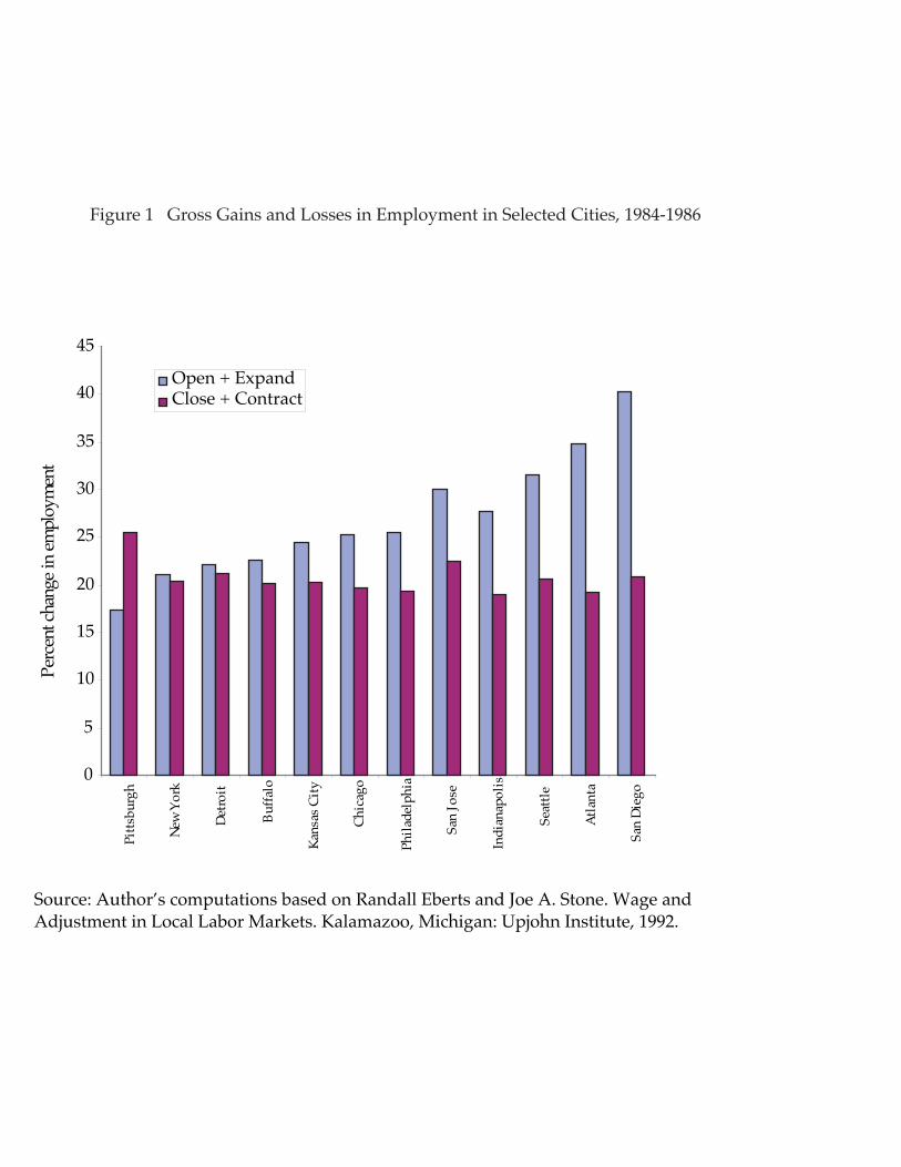
Figure 1 provides a useful backdrop for our discussion of location decisions and

urban growth. A city will grow if the number of new jobs gained from the birth of new

firms and the expansion of existing firms exceeds the number of old jobs lost from firm

deaths and contractions. The question is whether growing cities have relatively large job

gains, or relatively small job losses. The clear message from Figure 1 is that cities differ

Open + ExpandClose + Contract

0

5

10

15

20

25

30

35

40

45

Pitts

burg

h

New

York

Detro

it

Buffa

lo

Kans

asCi

ty

Chic

ago

Phila

delp

hia

San

Jose

Indi

anap

olis

Seat

tle

Atla

nta

San

Dieg

o

Perc

entc

hang

ein

empl

oym

ent

Source: Author’s computations based on Randall Eberts and Joe A. Stone. Wage andAdjustment in Local Labor Markets. Kalamazoo, Michigan: Upjohn Institute, 1992.

Figure 1 Gross Gains and Losses in Employment in Selected Cities, 1984-1986

in their job gains, not their job losses. Although most cities have roughly the same

percentage of job losses, growing cities have larger gains from births and expansions.

The location decisions of firms are based on profit maximization. A firm’s

potential profit varies across space for several reasons. First, it is costly to transport

inputs and outputs, and locations with relatively low transport costs will generate higher

profits, ceteris paribus (everything else being equal). Second, some inputs cannot be

transported at all, and locations with inexpensive local (nontransferable) inputs will

generate higher profits, ceteris paribus. Third, some firms benefit from proximity to other

firms in the same industry (localization economies) and other firms benefit from being in

a large diverse city (urbanization economies). Fourth, the public sector levies taxes and

provides public goods and services, and locations with a relatively efficient public sector

will generate higher profits, ceteris paribus.

TRANSFERABLE INPUTS AND OUTPUTS

A transfer-oriented firm is defined as one for which transportation cost is the

dominant factor in the location decision. The firm chooses the location that minimizes

total transport costs, defined as the sum of procurement and distribution costs.

Procurement cost is the cost of transporting raw materials from the input source to the

production facility. Distribution cost is the cost of transporting the firm’s output from the

production facility to the consumer.

The classic model of a transfer-oriented firm has four assumptions that focus

attention on transportation costs as the dominant location variable.

• Single transferable output. The firm produces a fixed quantity of a single

product, which is transported from the production facility to a market at point M.

• Single transferable input. The firm may use several inputs, but only one input is

transported from an input source (point F) to the firm’s production facility. All

other inputs are ubiquitous, meaning that they are available at all locations at the

same price.

• Fixed-factor proportions. The firm produces its fixed quantity with fixed

amounts of each input. In other words, the firm uses a single recipe to produce its

good, regardless of the prices of its inputs. There is no factor substitution.

• Fixed prices. The firm is so small that it does not affect the prices of its inputs or

its product.

Under these four assumptions, the firm maximizes its profit by minimizing its

transportation costs. The firm’s profit equals total revenue (price times the quantity of

output) less input costs and transport costs. Total revenue is the same at all locations

because the firm sells a fixed quantity of output at a fixed price. Input costs are the same

at all locations because the firm buys a fixed amount of each input at fixed prices. The

only costs that vary across space are procurement costs (the costs of transporting the

firm’s transferable input) and distribution costs (the costs of transporting the firm’s

output). Therefore, the firm will choose the location that minimizes its total transport

costs.

The firm’s location choice is determined by the outcome of a tug-of-war. The firm

is pulled toward its input source because the closer to the input source, the lower the

firm’s procurement costs. On the other side, the firm is pulled toward the market because

proximity to the market reduces the firm’s distribution costs.

Resource-Oriented Firms

A resource-oriented firm is defined as a firm that has relatively high costs for

transporting its input. Table 1 shows the transport characteristics for such a firm. The

firm produces baseball bats, using 10 tons of wood to produce 3 tons of bats. The firm is

involved in a weight-losing activity in the sense that its output is lighter than its

transferable input.

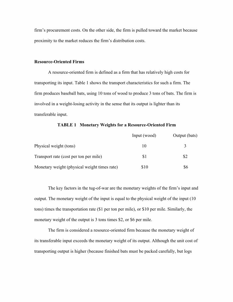
TABLE 1 Monetary Weights for a Resource-Oriented Firm

Input (wood) Output (bats)

Physical weight (tons) 10 3

Transport rate (cost per ton per mile) $1 $2

Monetary weight (physical weight times rate) $10 $6

The key factors in the tug-of-war are the monetary weights of the firm’s input and

output. The monetary weight of the input is equal to the physical weight of the input (10

tons) times the transportation rate ($1 per ton per mile), or $10 per mile. Similarly, the

monetary weight of the output is 3 tons times $2, or $6 per mile.

The firm is considered a resource-oriented firm because the monetary weight of

its transferable input exceeds the monetary weight of its output. Although the unit cost of

transporting output is higher (because finished bats must be packed carefully, but logs

can be tossed onto a truck), the loss of weight in the production process generates a lower

monetary weight for the output.

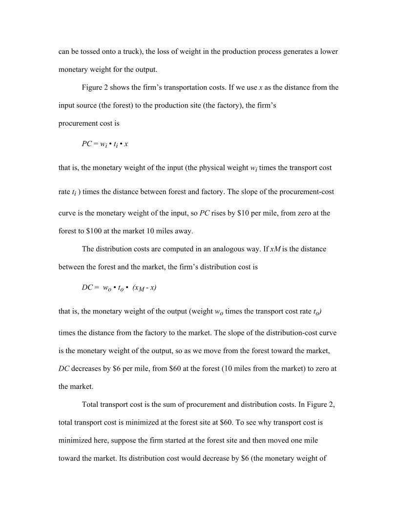
Figure 2 shows the firm’s transportation costs. If we use x as the distance from the

input source (the forest) to the production site (the factory), the firm’s

procurement cost is

PC = wi • ti • x

that is, the monetary weight of the input (the physical weight wi times the transport cost

rate ti ) times the distance between forest and factory. The slope of the procurement-cost

curve is the monetary weight of the input, so PC rises by $10 per mile, from zero at the

forest to $100 at the market 10 miles away.

The distribution costs are computed in an analogous way. If xM is the distance

between the forest and the market, the firm’s distribution cost is

DC = wo • to • (xM - x)

that is, the monetary weight of the output (weight wo times the transport cost rate to)

times the distance from the factory to the market. The slope of the distribution-cost curve

is the monetary weight of the output, so as we move from the forest toward the market,

DC decreases by $6 per mile, from $60 at the forest (10 miles from the market) to zero at

the market.

Total transport cost is the sum of procurement and distribution costs. In Figure 2,

total transport cost is minimized at the forest site at $60. To see why transport cost is

minimized here, suppose the firm started at the forest site and then moved one mile

toward the market. Its distribution cost would decrease by $6 (the monetary weight of

x (Distance from Forest)

Distribution Cost (DC)

80

100

2 4 6 8 10

$

Procurement Cost (PC)

Total Transport Cost = PC + DC

Forest (F)

Market (M)

Total Transport Cost (the sum of Procurement Cost and Distribution Cost) is minimized atthe forest because the monetary weight of the input ($10) exceeds the monetary weight ofthe output ($6). The weight-gaining activity locates at its source of raw materials.

20

40

60

Figure 2 Transport Costs for a Resource-Oriented Firm

bats) but its procurement cost would increase by $10 (the monetary weight of the wood),

so its total transport cost would increases by $4. The firm’s total transport cost is

minimized at the forest because the monetary weight of the input exceeds the monetary

weight of the output. The resource-oriented firm locates near its input source.

The bat firm is resource-oriented because it is a weight-losing activity, using 10

tons of wood to produce only three tons of bats. The cost of transporting wood is large

relative to the cost of transporting the finished output, so the firm saves on transport costs

by locating near the forest. In this case, the tug-of-war is won by the input source because

there is more physical weight on the input side. Here are some other examples of weight-

losing firms.

1. Beet-sugar factories locate near sugar-beet farms because one pound of sugar beets

generates only about 2.7 ounces of sugar.

2. Onion dehydrators locate near onion fields because one pound of fresh onions

becomes less than one pound of dried onions.

3. Ore processors locate near mines because they use only a fraction of the materials

extracted from the ground.

Some firms are resource oriented because their inputs are relatively expensive to

transport. Consider a firm that cans fruit, producing one ton of canned fruit with roughly

a ton of raw fruit. The firm’s input is perishable, and must be transported in refrigerated

trucks, while its output can be transported less expensively on regular trucks. Because the

cost of shipping a ton of raw fruit exceeds the cost of shipping a ton of canned fruit, the

monetary weight of the input exceeds the monetary weight of the output, and the firm

will locate near its input source, a fruit farm.

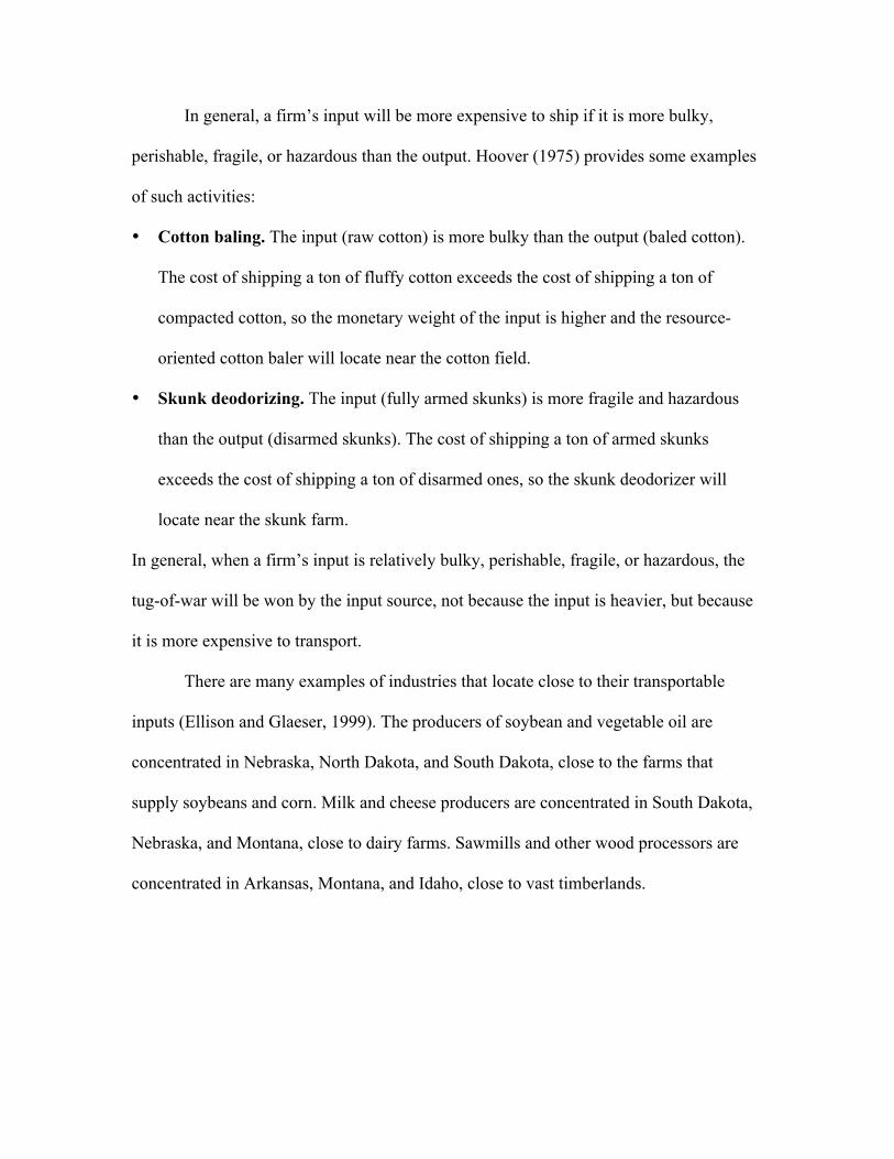
In general, a firm’s input will be more expensive to ship if it is more bulky,

perishable, fragile, or hazardous than the output. Hoover (1975) provides some examples

of such activities:

• Cotton baling. The input (raw cotton) is more bulky than the output (baled cotton).

The cost of shipping a ton of fluffy cotton exceeds the cost of shipping a ton of

compacted cotton, so the monetary weight of the input is higher and the resource-

oriented cotton baler will locate near the cotton field.

• Skunk deodorizing. The input (fully armed skunks) is more fragile and hazardous

than the output (disarmed skunks). The cost of shipping a ton of armed skunks

exceeds the cost of shipping a ton of disarmed ones, so the skunk deodorizer will

locate near the skunk farm.

In general, when a firm’s input is relatively bulky, perishable, fragile, or hazardous, the

tug-of-war will be won by the input source, not because the input is heavier, but because

it is more expensive to transport.

There are many examples of industries that locate close to their transportable

inputs (Ellison and Glaeser, 1999). The producers of soybean and vegetable oil are

concentrated in Nebraska, North Dakota, and South Dakota, close to the farms that

supply soybeans and corn. Milk and cheese producers are concentrated in South Dakota,

Nebraska, and Montana, close to dairy farms. Sawmills and other wood processors are

concentrated in Arkansas, Montana, and Idaho, close to vast timberlands.

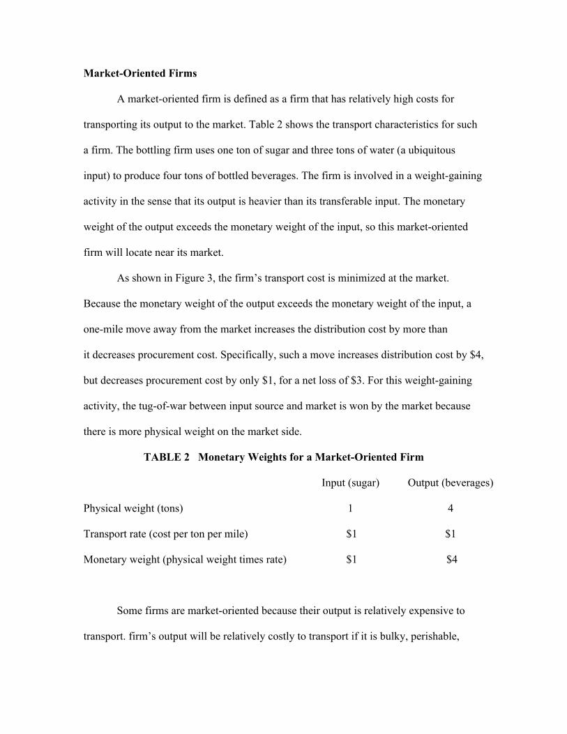
Market-Oriented Firms

A market-oriented firm is defined as a firm that has relatively high costs for

transporting its output to the market. Table 2 shows the transport characteristics for such

a firm. The bottling firm uses one ton of sugar and three tons of water (a ubiquitous

input) to produce four tons of bottled beverages. The firm is involved in a weight-gaining

activity in the sense that its output is heavier than its transferable input. The monetary

weight of the output exceeds the monetary weight of the input, so this market-oriented

firm will locate near its market.

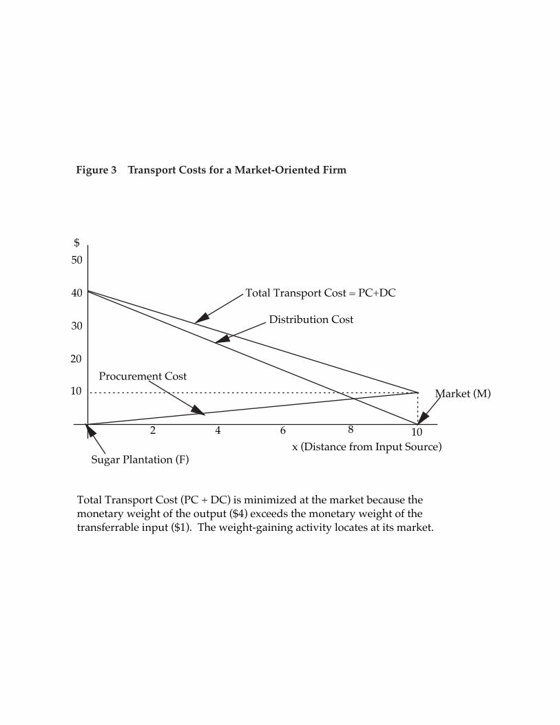
As shown in Figure 3, the firm’s transport cost is minimized at the market.

Because the monetary weight of the output exceeds the monetary weight of the input, a

one-mile move away from the market increases the distribution cost by more than

it decreases procurement cost. Specifically, such a move increases distribution cost by $4,

but decreases procurement cost by only $1, for a net loss of $3. For this weight-gaining

activity, the tug-of-war between input source and market is won by the market because

there is more physical weight on the market side.

TABLE 2 Monetary Weights for a Market-Oriented Firm

Input (sugar) Output (beverages)

Physical weight (tons) 1 4

Transport rate (cost per ton per mile) $1 $1

Monetary weight (physical weight times rate) $1 $4

Some firms are market-oriented because their output is relatively expensive to

transport. firm’s output will be relatively costly to transport if it is bulky, perishable,

Distribution Cost

10

20

30

40

50

2 4 6 8 10

$

Total Transport Cost = PC+DC

x (Distance from Input Source)Sugar Plantation (F)

Market (M)

Total Transport Cost (PC + DC) is minimized at the market because themonetary weight of the output ($4) exceeds the monetary weight of thetransferrable input ($1). The weight-gaining activity locates at its market.

Procurement Cost

Figure 3 Transport Costs for a Market-Oriented Firm

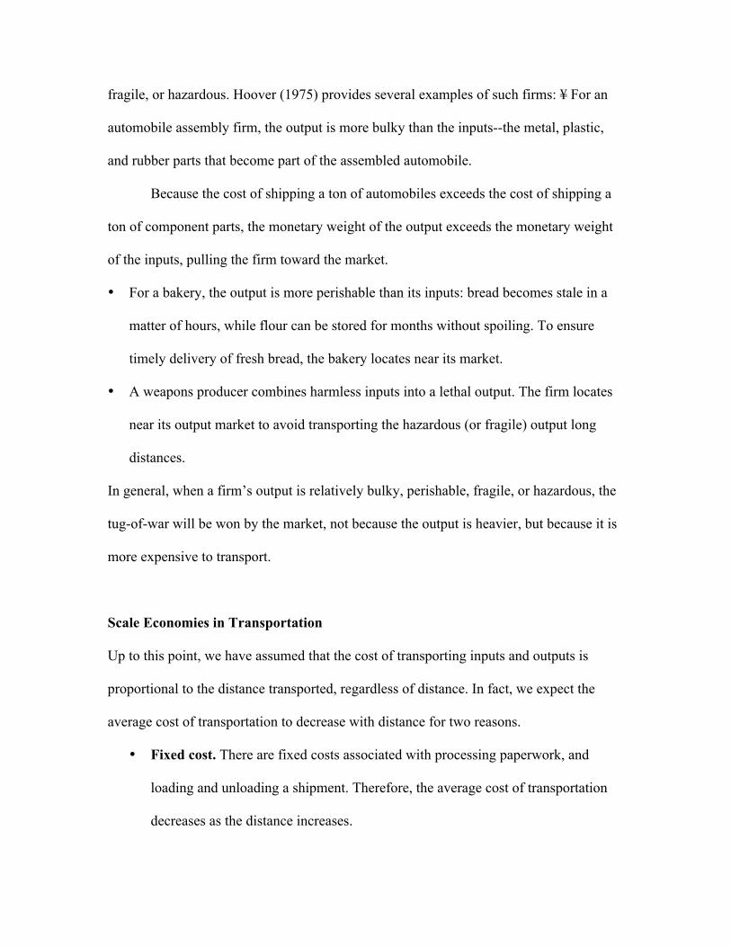
fragile, or hazardous. Hoover (1975) provides several examples of such firms: ¥ For an

automobile assembly firm, the output is more bulky than the inputs--the metal, plastic,

and rubber parts that become part of the assembled automobile.

Because the cost of shipping a ton of automobiles exceeds the cost of shipping a

ton of component parts, the monetary weight of the output exceeds the monetary weight

of the inputs, pulling the firm toward the market.

• For a bakery, the output is more perishable than its inputs: bread becomes stale in a

matter of hours, while flour can be stored for months without spoiling. To ensure

timely delivery of fresh bread, the bakery locates near its market.

• A weapons producer combines harmless inputs into a lethal output. The firm locates

near its output market to avoid transporting the hazardous (or fragile) output long

distances.

In general, when a firm’s output is relatively bulky, perishable, fragile, or hazardous, the

tug-of-war will be won by the market, not because the output is heavier, but because it is

more expensive to transport.

Scale Economies in Transportation

Up to this point, we have assumed that the cost of transporting inputs and outputs is

proportional to the distance transported, regardless of distance. In fact, we expect the

average cost of transportation to decrease with distance for two reasons.

• Fixed cost. There are fixed costs associated with processing paperwork, and

loading and unloading a shipment. Therefore, the average cost of transportation

decreases as the distance increases.

• Line-haul economies. The transport cost per mile decreases as the distance

increases, reflecting the efficiencies from using different modes for different

distances. A firm may use a truck for a short haul, but a train or a ship for a long

haul. The unit transport cost is lower for trains and ships, so the average cost

decreases as distance increases.

The presence of scale economies in transportation reinforces the tendency for a

firm to locate at either its input sources or its markets. In the absence of scale economies,

if the monetary weight of the output equals the monetary weight of the input, the firm

would be indifferent between the two locations and any points in between, and could

choose some location in the middle. But if there are scale economies in transportation, it

would not be sensible to locate anywhere between the two points. It will be more efficient

to make one long trip (transporting either the input or the output) instead of two short

trips (transporting both the input and the output).

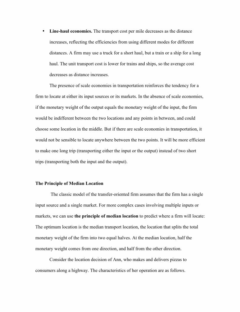
The Principle of Median Location

The classic model of the transfer-oriented firm assumes that the firm has a single

input source and a single market. For more complex cases involving multiple inputs or

markets, we can use the principle of median location to predict where a firm will locate:

The optimum location is the median transport location, the location that splits the total

monetary weight of the firm into two equal halves. At the median location, half the

monetary weight comes from one direction, and half from the other direction.

Consider the location decision of Ann, who makes and delivers pizzas to

consumers along a highway. The characteristics of her operation are as follows.

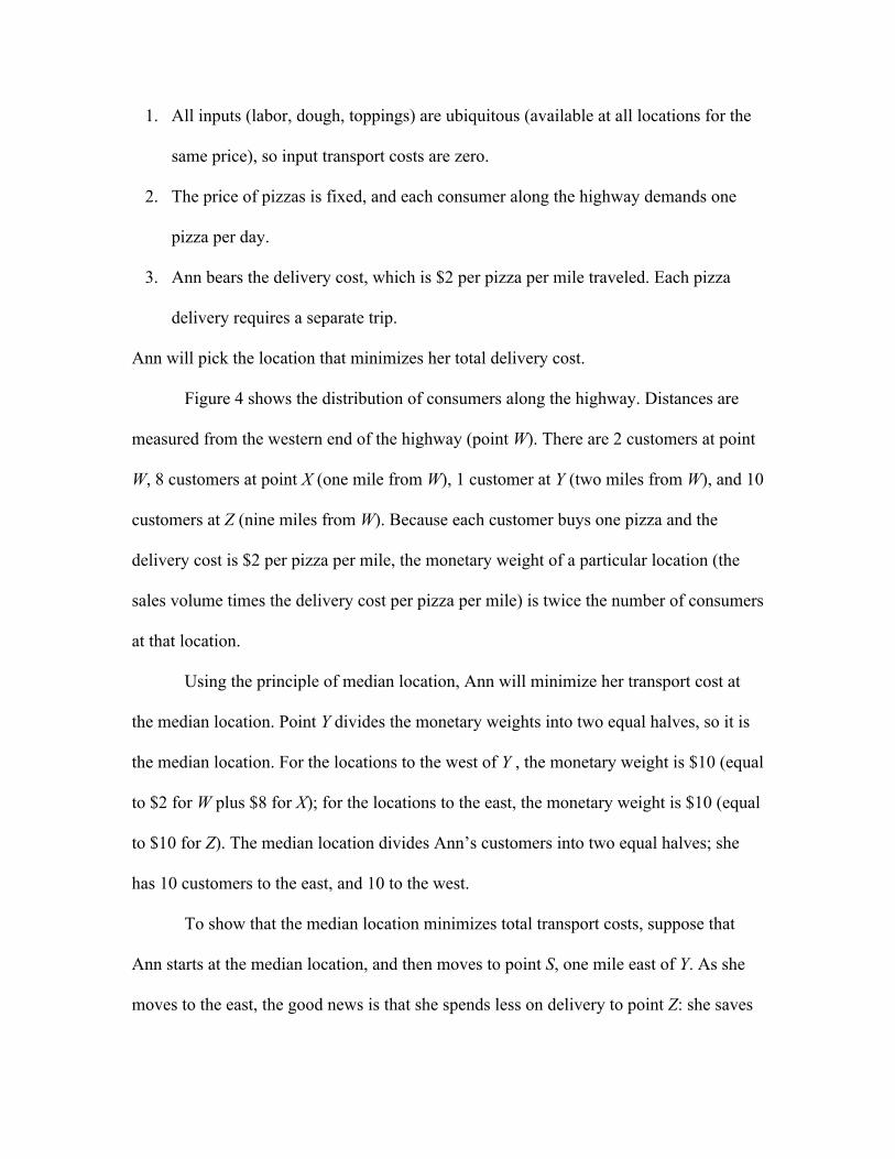
1. All inputs (labor, dough, toppings) are ubiquitous (available at all locations for the

same price), so input transport costs are zero.

2. The price of pizzas is fixed, and each consumer along the highway demands one

pizza per day.

3. Ann bears the delivery cost, which is $2 per pizza per mile traveled. Each pizza

delivery requires a separate trip.

Ann will pick the location that minimizes her total delivery cost.

Figure 4 shows the distribution of consumers along the highway. Distances are

measured from the western end of the highway (point W). There are 2 customers at point

W, 8 customers at point X (one mile from W), 1 customer at Y (two miles from W), and 10

customers at Z (nine miles from W). Because each customer buys one pizza and the

delivery cost is $2 per pizza per mile, the monetary weight of a particular location (the

sales volume times the delivery cost per pizza per mile) is twice the number of consumers

at that location.

Using the principle of median location, Ann will minimize her transport cost at

the median location. Point Y divides the monetary weights into two equal halves, so it is

the median location. For the locations to the west of Y , the monetary weight is $10 (equal

to $2 for W plus $8 for X); for the locations to the east, the monetary weight is $10 (equal

to $10 for Z). The median location divides Ann’s customers into two equal halves; she

has 10 customers to the east, and 10 to the west.

To show that the median location minimizes total transport costs, suppose that

Ann starts at the median location, and then moves to point S, one mile east of Y. As she

moves to the east, the good news is that she spends less on delivery to point Z: she saves

W X Y S Z

Distance From W

Number of Consumers

Monetary Weight

0 1 2 9

2 8 1 10

$4 $16 $2 $20

3

Ann locates her pizza parlor at point Y because it is the median location: she delivers10 pizza to consumers to the west of Y, and 10 to consumers tothe east of Y. Amove from Y to S would decrease delivery cost for the 10 consumers at point E(savings of $20), but increase delivery costs for the 11 consumers at points W, X, andY (increase in cost of $22). A move in the opposite direction would also increasetotal transport costs.

Figure 4 The Principle of Median Location

$2 per trip to Z, saving a total of $10 in eastward delivery costs. The bad news is that

westward costs increase: she pays $2 more per trip to points W, X, and Y ; since there are

11 customers to the west of S, her westward delivery costs increase by a total of $22 ($4

for W, $16 for X, and $2 for Y ). Since the increase in westward costs exceeds the

decrease in eastward costs, the move from Y to S increases total delivery costs. The same

is true for a move in the opposite direction; if Ann moves from Y toward W, her delivery

costs will increase.

The median location minimizes total transport costs because it splits pizza

consumers into two equal parts. As Ann moves eastward away from Y , she moves further

away from 11 customers, but moves closer to only 10 customers. Similarly, a westward

move will cause her to move closer to 10 customers, but further from 11 customers. In

general, any move away from the median location will increase delivery costs for the

majority of consumers, so total delivery cost increases. It is important to note that the

distance between the consumers is irrelevant to the firm’s location choice. For example,

if the Z consumers were located 100 miles from W instead of 9 miles from W, the median

location would still be point Y . Total delivery costs would still be minimized (at a higher

level, of course) at point Y .

The principle of median location provides another explanation of why large cities

become larger. Consider a firm that delivers its product to consumers in five different

cities. In Figure 5, there is a large city at location L, and four small cities at locations S1,

S2, S3, and S4. The firm sells 4 units in each small city, and 17 units in the large city. The

median location is in the large city, even though the large city is at the end of the line. A

one-mile move westward from L would decrease transport costs by $16 (as the firm

moved closer to consumers in the small cities), but would increase transport costs by $17

(as the firm moved away from consumers in the large city). The lesson from this example

is that the concentration of demand in large cities causes large cities to grow.

Transshipment Points and Port Cities

The principle of median location also explains why some industrial firms locate at

transshipment points. A transshipment point is defined as a point at which a good is

transferred from one transport mode to another. At a port, goods are transferred from

trucks or trains to ships; at a railroad terminal, goods are transferred from trucks to the

train.

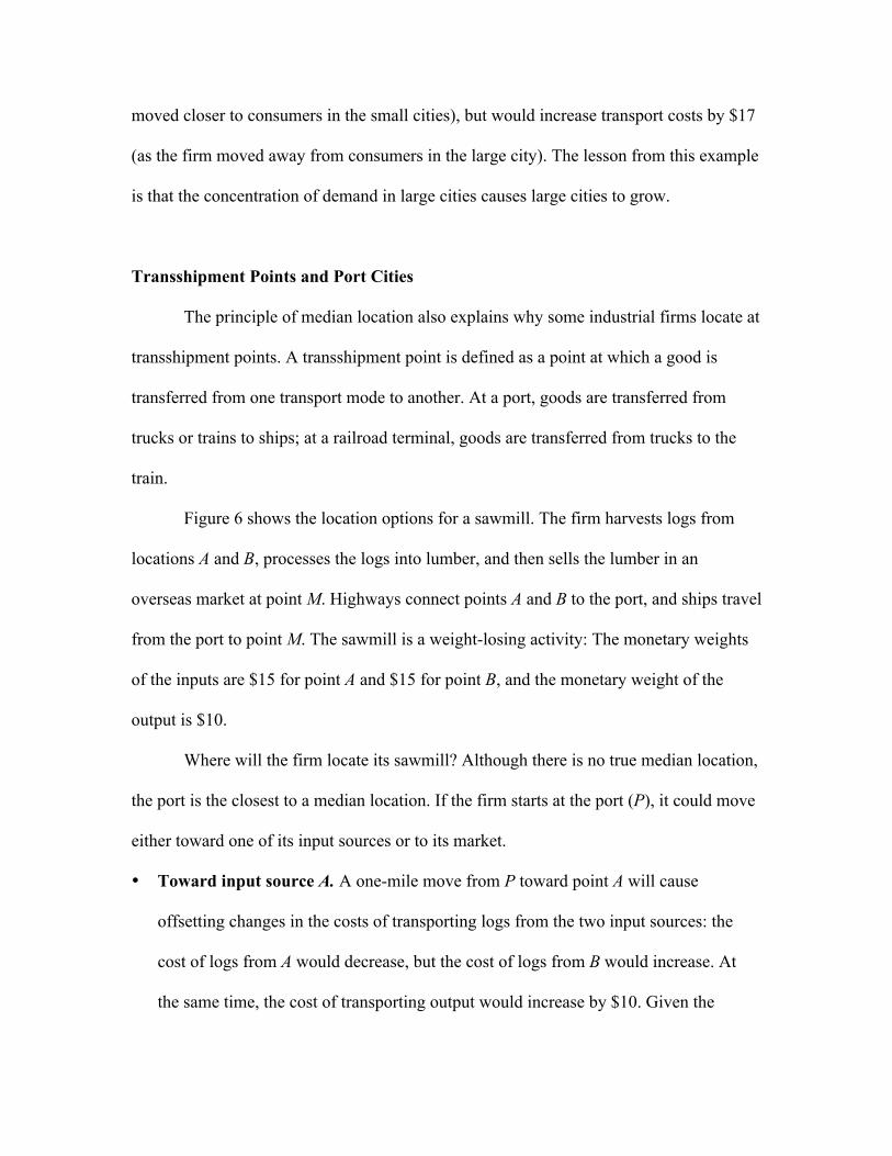
Figure 6 shows the location options for a sawmill. The firm harvests logs from

locations A and B, processes the logs into lumber, and then sells the lumber in an

overseas market at point M. Highways connect points A and B to the port, and ships travel

from the port to point M. The sawmill is a weight-losing activity: The monetary weights

of the inputs are $15 for point A and $15 for point B, and the monetary weight of the

output is $10.

Where will the firm locate its sawmill? Although there is no true median location,

the port is the closest to a median location. If the firm starts at the port (P), it could move

either toward one of its input sources or to its market.

• Toward input source A. A one-mile move from P toward point A will cause

offsetting changes in the costs of transporting logs from the two input sources: the

cost of logs from A would decrease, but the cost of logs from B would increase. At

the same time, the cost of transporting output would increase by $10. Given the

Input Source A

Input Source B

M P

PortOutput Market

The firm locates its sawmill at the port (P) because it is the median transportlocation. A move from P toward either A or B would increase output transport costsby $10 without affecting input transport costs. A move from P toward M wouldincrease input transport costs by $30 but decrease output transport costs by only$10.

Monetary weight = $15

Monetary weight = $15

Monetary weight = $10

Figure 6 Median Location and Ports

offsetting changes in input transport costs and the increase in output costs, the port

location is superior to locations between P and A. The same argument applies for a

move from P toward B.

• To market (M). Unless the firm wants to operate a floating sawmill, it would not

move to points between the port and the overseas market at M. It could, however,

move all the way to the market. A move from P to M would decrease output transport

cost by $10 (the monetary weight of output) times the distance between M and P, and

increase input transport cost by $30 (the monetary weight of the inputs) times the

distance. Therefore, the port location is superior to the market location.

Although the sawmill is a weight-losing activity, it will locate at the port, not at

one of its input sources. The port location is efficient because it provides a central

collection point for the firm’s inputs.

There are many examples of port cities that developed as a result of the location

decisions of industrial firms. Seattle started in 1880 as a sawmill town: Firms harvested

trees in western Washington, processed the logs in Seattle sawmills, and then shipped the

wood products to other states and countries. Baltimore was the nation’s first boomtown:

Flour mills processed wheat from the surrounding agricultural areas for export to the

West Indies. Buffalo was the Midwestern center for flour mills, providing consumers in

eastern cities with flour produced from Midwestern wheat. Wheat was shipped from

Midwestern states across the Great Lakes to Buffalo, where it was processed into flour

for shipment, by rail, to cities in the eastern United States. In contrast with Baltimore,

which exported its output (flour) by ship, Buffalo imported its input (wheat) by ship.

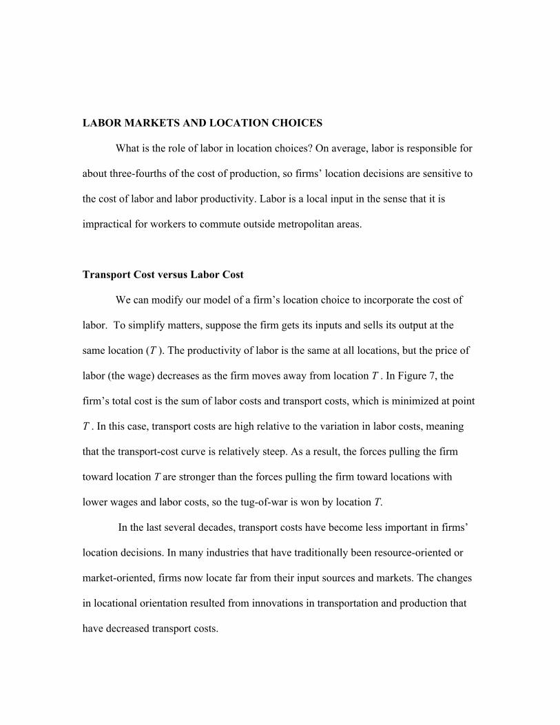
LABOR MARKETS AND LOCATION CHOICES

What is the role of labor in location choices? On average, labor is responsible for

about three-fourths of the cost of production, so firms’ location decisions are sensitive to

the cost of labor and labor productivity. Labor is a local input in the sense that it is

impractical for workers to commute outside metropolitan areas.

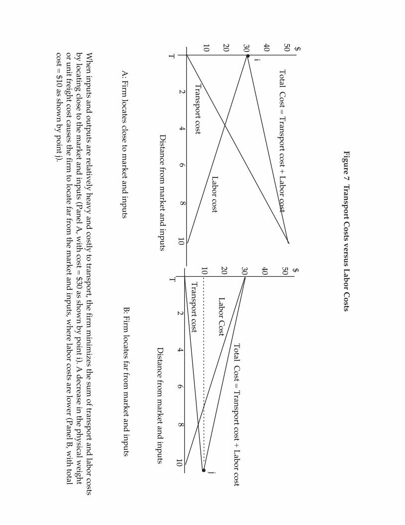
Transport Cost versus Labor Cost

We can modify our model of a firm’s location choice to incorporate the cost of

labor. To simplify matters, suppose the firm gets its inputs and sells its output at the

same location (T ). The productivity of labor is the same at all locations, but the price of

labor (the wage) decreases as the firm moves away from location T . In Figure 7, the

firm’s total cost is the sum of labor costs and transport costs, which is minimized at point

T . In this case, transport costs are high relative to the variation in labor costs, meaning

that the transport-cost curve is relatively steep. As a result, the forces pulling the firm

toward location T are stronger than the forces pulling the firm toward locations with

lower wages and labor costs, so the tug-of-war is won by location T.

In the last several decades, transport costs have become less important in firms’

location decisions. In many industries that have traditionally been resource-oriented or

market-oriented, firms now locate far from their input sources and markets. The changes

in locational orientation resulted from innovations in transportation and production that

have decreased transport costs.

Labor cost10 20 30 40 50

24

68

10

$

Total Cost = Transport cost + Labor cost

Distance from

market and inputs

Transport cost

Labor Cost

10 20 30 40 50

24

68

10

$

Total Cost = Transport cost + Labor cost

T Transport cost

Distance from

market and inputs

T

A: Firm

locates close to market and inputs

B: Firm locates far from

market and inputs

i

j

When inputs and outputs are relatively heavy and costly to transport, the firm

minim

izes the sum of transport and labor costs

by locating close to the market and inputs (Panel A

, with cost = $30 as show

n by point i). A decrease in the physical w

eightor unit freight cost causes the firm

to locate far from the m

arket and inputs, where labor costs are low

er (Panel B, with total

cost = $10 as shown by point j).

Figure 7 Transport Costs versus Labor C

osts

• Transportation technology. The development of fast ocean ships and container

technology decreased shipping costs, while improvements in railroads and trucks

lowered the cost of overland travel. Faster and more efficient aircraft have decreased

the cost of air travel.

• Production technology. Improvements in production techniques decreased the

physical weight of inputs. For example, the amount of coal and ore required to

produce one ton of steel has decreased steadily, a result of improved production

methods and the use of scrap metal (a local input) instead of iron ore (a transportable

input).

Panel B of Figure 7 shows the effects of a decrease in the unit transport costs and

the physical weights of inputs. These changes flatten the transport-cost curve, shifting the

cost-minimizing location to a location 10 miles from the market and inputs, where labor

costs are lower. The decrease in transport costs causes the firm to switch from transfer

orientation to labor orientation.

As unit transport costs and input weights decrease, firms are more likely to base

their location decisions on access to inexpensive local inputs rather than access to

transportable inputs. A recent example is the movement of the assembly operations of

many U.S. manufacturers to sites along the Mexican border. The steel industry has

moved from the eastern United States, with its rich coal and ore deposits, to Brazil,

Korea, and Mexico--far from both raw materials and steel markets. Similarly,

manufacturers have moved from the United States to Asia and Mexico, far from U.S.

markets, because the savings in labor costs are greater than the increase in transport costs.

Labor in the Long Run

In the long run, workers can move between cities. In the typical year, about 6

percent of the U.S. population move across county lines, and about 3 percent move across

state borders (Black, 2000). A firm that locates in one city could hire workers currently

living in another city with the expectation that the workers will transfer to the firm’s city.

According to Bartik (1991), the vast majority of new jobs in cities are filled with people

who relocate from other cities: When the number of jobs in a city increases by 1,000, on

average, only 230 jobs go to current residents; the rest go to workers who transfer from

other cities.

Labor and Natural Amenities

Consider a nation that has two regions--with warm weather in the North and cold

weather in the South--and workers prefer warm weather. To achieve locational

equilibrium for workers, wages in the South must be lower than wages in the North;

otherwise, there would be an incentive for workers to move to the South, getting the same

wage and better weather as well. In equilibrium, the wage for a given skill level will be

lower in the South, and northern workers will be compensated for bad weather by a

higher wage.

The lower wage caused by weather will encourage firms to locate their production

facilities in the South. In this case, the local nature of weather and workers’ preference

for warm weather makes labor a local input. The firm’s location depends on the location

choice of its workforce: instead of workers following firms, firms follow workers. Graves

(1979) and Porell (1982) provide empirical support for this phenomenon. There is

evidence that weather has played an important role in location decisions and urban

growth. In the past few decades, the most rapidly growing urban areas are ones with

warm, dry weather (Black and Henderson, 1999; Glaeser, Kolko, and Saiz, 2001).

Natural amenities appear to be most important for firms that employ high-income

workers. Since the demands for these amenities are income-elastic, high-income workers

are attracted to locations with amenities, and the firms hiring these people follow. For

example, research and development firms employ engineers and computer scientists, who

place a high value on good weather and a clean environment.

One explanation for the shift of employment from northern states to the southern

and western states is that rising income has increased the demand for natural amenities,

causing workers to move to areas that provide these amenities.

CASE STUDIES AND EMPIRICAL RESULTS

This section discusses some of the facts on the location choices of firms. We’ll

look at case studies of the location decisions of companies in the semiconductor industry,

Japanese and American auto firms, Mexican garment manufacturers, and the carpet

industry. We’ll also discuss empirical evidence concerning the effects of labor costs and

unions on location decisions.

The Semiconductor Industry

The semiconductor industry illustrates some of the complexities of locational

choices in modern industry. The industry’s output is light and compact relative to its

value, so transport costs are relatively unimportant in location decisions. What matters

are localization economies and access to different types of labor.

As explained by Castells (1988), the making of semiconductors involves several

distinct operations, requiring three different types of labor:

1. Research and development. Engineers and scientists design new circuits and prepare

the circuits for implantation into silicon chips.

2. Wafer fabrication. Skilled technicians and manual workers make the chips holding

the circuits.

3. Assembly into components. Unskilled workers assemble the chips into electronic

components.

Many semiconductor firms split their operations into three parts. Research and

development occurs in the Silicon Valley to exploit localization economies generated by

the large concentration of semiconductor firms. The Silicon Valley is also considered a

desirable location by engineers and scientists. Advanced manufacturing (wafer

production) is typically located outside the Silicon Valley. For example, National

Semiconductor has manufacturing facilities in Utah, Arizona, and the state of

Washington; Intel has plants in Oregon, Arizona, and Texas; and Advanced Micro

Devices has a plant in Texas. These facilities are located in areas that provide (1) a

plentiful supply of skilled manual laborers, (2) an environment attractive to engineers and

technicians, and (3) easy access, by air transportation, to the Silicon Valley. The firm’s

assembly facilities are typically overseas, in locations such as Southeast Asia that provide

a plentiful supply of low-skilled workers.

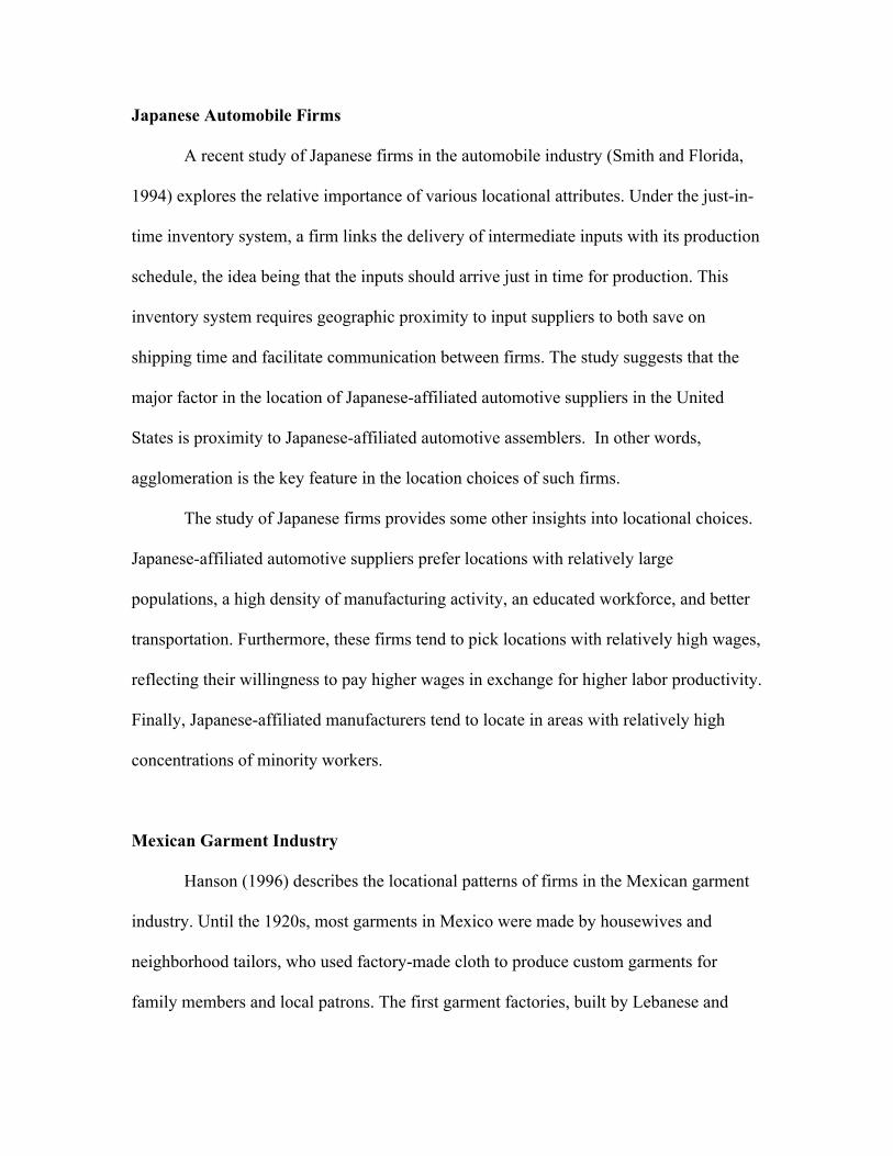
Japanese Automobile Firms

A recent study of Japanese firms in the automobile industry (Smith and Florida,

1994) explores the relative importance of various locational attributes. Under the just-in-

time inventory system, a firm links the delivery of intermediate inputs with its production

schedule, the idea being that the inputs should arrive just in time for production. This

inventory system requires geographic proximity to input suppliers to both save on

shipping time and facilitate communication between firms. The study suggests that the

major factor in the location of Japanese-affiliated automotive suppliers in the United

States is proximity to Japanese-affiliated automotive assemblers. In other words,

agglomeration is the key feature in the location choices of such firms.

The study of Japanese firms provides some other insights into locational choices.

Japanese-affiliated automotive suppliers prefer locations with relatively large

populations, a high density of manufacturing activity, an educated workforce, and better

transportation. Furthermore, these firms tend to pick locations with relatively high wages,

reflecting their willingness to pay higher wages in exchange for higher labor productivity.

Finally, Japanese-affiliated manufacturers tend to locate in areas with relatively high

concentrations of minority workers.

Mexican Garment Industry

Hanson (1996) describes the locational patterns of firms in the Mexican garment

industry. Until the 1920s, most garments in Mexico were made by housewives and

neighborhood tailors, who used factory-made cloth to produce custom garments for

family members and local patrons. The first garment factories, built by Lebanese and

Jewish immigrants, were located in downtown Mexico City. For several decades, the

industry was highly concentrated in the Federal District (the area containing Mexico

City), with about 60 percent of Mexico’s garment jobs there.

During the 1970s and 1980s, garment employment in the Federal District

decreased in relative and absolute terms. The district’s share of national garment

employment dropped from 60 percent in 1965 to 33 percent by 1985, with jobs moving to

states with lower wages (Aguascalientes, Jalisco, Mexico, Nuevo Leon, and Puebla).

Each state specialized in a particular type of garment, and garment employment in each

state is concentrated in one or two cities. For example, the city of Aguascalientes is the

employment center for children’s outerwear, with over 44 percent of the national

employment in that sector.

Although many garment jobs moved out of the Federal District, the district

retained its role as the center for marketing and design. In 1980, about 70 percent of the

wholesale trade in garments, textiles, and leather goods was conducted in the Federal

District, suggesting that the bulk of marketing and design still happens there.

Most of the jobs that moved to the outlying areas were low-skill assembly jobs. In

other words, there is a hierarchy of functions, with the activities subject to large

agglomerative economies (marketing and design) concentrated in one location, and

activities with smaller agglomerative economies (assembly) dispersed to outlying areas.

Carpet Manufacturing and Localization Economies

As an example of localization economies, consider Dalton, Georgia, the

preeminent carpet manufacturing center of the United States (Krugman, 1991). In 1895,

Catherine Evans of Dalton used an outdated technique--known as tufting or candle

wicking--to make a bedspread as a wedding gift. The gift was a big hit, and in the next

few years, Ms. Evans made a few tufted items for her friends and even sold a few. After

she discovered a few production tricks such as a technique for locking the tufts onto the

backing, she and her neighbors launched a local handicraft industry, producing handmade

tufted items for sale.

Immediately after World War II, a machine for producing tufted carpets was

developed, making tufted carpet a cheaper alternative to woven carpet. New carpet

makers sprung up in the Dalton area because that’s where they could find workers 86

with knowledge and experience in tufting. Support firms located nearby, supplying dyes,

backing, and other intermediate inputs. Some of the old firms that had produced woven

carpets went out of business because they were underpriced by tufting firms, while others

moved from the Northeast to the Dalton area and switched to the new technique. By the

middle of the 1950s, Dalton was the carpet capital of the nation. Of the top 20 carpet

manufacturers in the United States, 6 are located in Dalton, and 13 others are located

nearby.

GM’s Saturn Plant

In 1985, General Motors announced that its new Saturn plant would be located in

Spring Hill, Tennessee, a crossroads community about 30 miles from Nashville. The

plant, which cost several billions of dollars to build, employs about 3,000 workers and

supports thousands of jobs in the Nashville area. Why did GM choose Nashville over the

dozens of other communities that sought the plant?

A case study by Bartik, Becker, Lake, and Bush (1987) explored differences in

transportation, labor costs, and taxes for alternative locations. The first step in the case

study addressed the issue of transportation costs and market access. The authors

estimated the costs of shipping finished cars from seven alternative production sites to

GM’s markets in the continental United States. Based on the distribution of projected

sales in 2000, the location offering the best market access was Terre Haute, Indiana.

As shown in Table 3, the variation in transportation cost among the seven sites

was relatively small. The gap between Terre Haute and the site with the highest

transportation cost (Kalamazoo) was only $17 per car. Nashville was ranked fifth, with

transport costs only $13 per car higher than Terre Haute.

The second step of the study incorporated labor costs into the analysis. A labor

contract between GM and its unionized workers stipulated that the Saturn workers will be

paid the same wage regardless of the plant’s location, so GM would not decrease its own

wage bill by locating in Tennessee, a state with low wages. However, GM would

purchase a large fraction of its inputs from nearby suppliers, who would pay low wages

and pass on the savings to GM. As shown in Table 3, the variation in labor cost was

relatively large. The difference between the lowest-cost site (Nashville) and the highest-

cost site (Kalamazoo) was $85 per car.

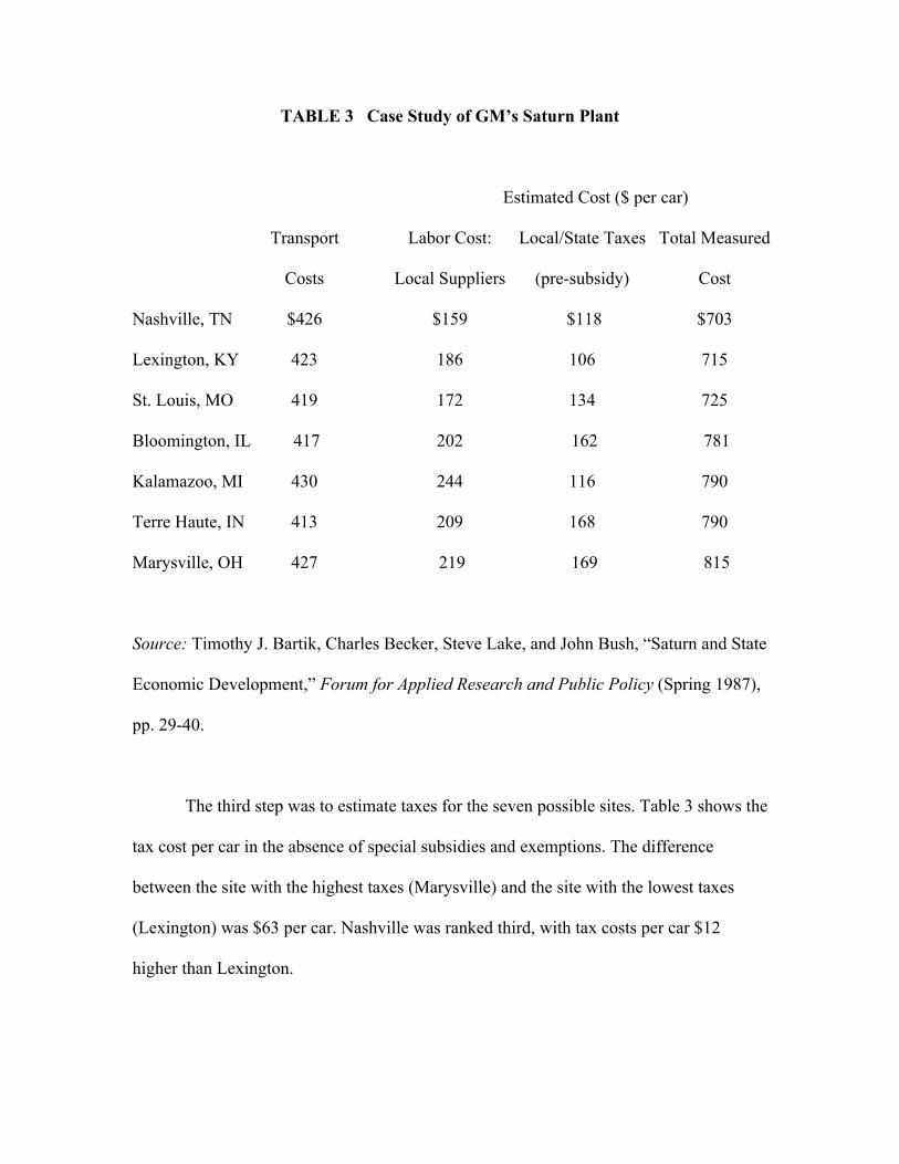
TABLE 3 Case Study of GM’s Saturn Plant

Estimated Cost ($ per car)

Transport Labor Cost: Local/State Taxes Total Measured

Costs Local Suppliers (pre-subsidy) Cost

Nashville, TN $426 $159 $118 $703

Lexington, KY 423 186 106 715

St. Louis, MO 419 172 134 725

Bloomington, IL 417 202 162 781

Kalamazoo, MI 430 244 116 790

Terre Haute, IN 413 209 168 790

Marysville, OH 427 219 169 815

Source: Timothy J. Bartik, Charles Becker, Steve Lake, and John Bush, “Saturn and State

Economic Development,” Forum for Applied Research and Public Policy (Spring 1987),

pp. 29-40.

The third step was to estimate taxes for the seven possible sites. Table 3 shows the

tax cost per car in the absence of special subsidies and exemptions. The difference

between the site with the highest taxes (Marysville) and the site with the lowest taxes

(Lexington) was $63 per car. Nashville was ranked third, with tax costs per car $12

higher than Lexington.

This case study suggests that in the absence of special tax treatment, Nashville

had the lowest total cost. The most important factor was the lower labor costs in

Nashville. Although the city had a slight disadvantage to Terre Haute in terms of market

access, this disadvantage was more than offset by Nashville’s lower labor costs.

The state of Tennessee offered three types of inducements to GM. The first was a

$30 million highway project that connected the plant with Interstate 65. The second was a

subsidized job-training program for Saturn workers, worth about $4 per car. The third

was a program of property tax subsidies, worth about $30 per car. As shown by the

numbers in Table 3, these subsidies would not have been necessary in the absence of

special subsidies from other states. Other states did offer special subsidies, and Tennessee

responded in kind to stay competitive in the bidding for the plant.

Effects of Wages and Unions

How do wages affect firms location decisions? Carlton (1983) examines the

relationship between the number of new firms in a metropolitan area and several

variables, including local wages. He looks at firm births in three industries: plastics

products, electronic transmitting equipment, and electronic components. These industries

have relatively low transport costs, so they are oriented toward local inputs, not toward

output markets or natural resources. His results suggest that for the electronic

components industry the elasticity of the number of plant births with respect to the

metropolitan wage is -1.07. In other words, a 10 percent increase in the wage decreases

the number of births by 10.7 percent. Bartik (1991) examines and summarizes the results

of dozens of studies and concludes that the long-run elasticity of business activity with

respect to the wage is between -1.0 and -2.0. This means that a 10 percent decrease in the

metropolitan wage will increase business activity between 10 percent and 20 percent.

How do unions affect location decisions and the volume of business activity?

One of the effects of unions is to increase wages, so a highly unionized metropolitan area

is likely to have relatively high wages. Since the elasticity of business activity with

respect to the wage is relatively large, to the extent that unions increase wages, they

decrease business activity. Unions may have other (nonwage) effects that influence

business location decisions. For example, unions may affect labor productivity.

According to Bartik (1991), empirical studies of the nonwage effects of unions

have generated mixed results. Although most studies found that the presence of unions

decreases business activity, many studies suggested that the negative effects are rather

small.

SUMMARY

1. Cities develop around the concentrations of employment generated by firms, so the

location choices of firms determine the location of cities and urban growth.

2. A resource-oriented firm has relatively high transport costs for its inputs, so it locates

near its input source.

3. A market-oriented firm has relatively high transport costs for its output, so it locates

close to its market.

4. A market-oriented firm with multiple inputs and outputs will locate at its median

transport location. The median location is often in large cities, providing one reason

for the growth of big cities.

5. Some firms are oriented toward local inputs. Energy-intensive firms are drawn toward

locations with cheap energy, while firms that benefit from agglomeration economies

are pulled toward industry clusters or large cities.

6. In the last several decades, the relative importance of transport costs has decreased,

reflecting decreases in unit transport costs and the physical weight of inputs.

7. Natural amenities attract workers, and the resulting lower wages attract firms.

EXERCISES AND DISCUSSION QUESTIONS

1. Comment on the following from the owner of a successful plywood mill: “Firms don’t

use location theory to make location decisions. I chose this location for my plywood mill

because it is close to my favorite fishing spot.”

2. Depict graphically the effects of the following changes on the bat firm’s cost curves

(shown in Figure 2). Explain any changes in the optimum location.

a. The cost of shipping bats increases from $1 per ton to $4 per ton, while the cost of

shipping wood remains at $1 per ton.

b. The forest at point F burns down, forcing the firm to use wood from point G which is

10 miles west of point F (20 miles from the market).

c. The firm starts producing bats with wood and cork, using three tons of wood and two

tons of cork to produce three tons of bats. Cork is ubiquitous (available at all locations for

the same price).

3. Why do breweries typically locate near their markets (far from their input sources),

while wineries typically locate near their input sources (far from their markets)?

4. The building of wooden ships was a weight-losing activity, as evidenced by the piles

of scrap wood generated by shipbuilders. Yet shipbuilders located in ports, far from their

input sources (inland forests). Why?

5. Consider a firm that delivers video rentals to its customers. The spatial distribution of

customers is as follows: 10 videos are delivered to location W, 10 miles due west of the

city center; 50 videos are delivered to the city center; 25 videos are delivered to E, 1 mile

due east of the city center; and 45 videos are delivered to point F, 2 miles east of the city

center. Production costs are the same at all locations.

a. Using a graph, show where the firm should locate. Explain your location choice.

b. Suppose that point W is in a valley and point F is at the top of a mountain.

Therefore, the unit cost of easterly transport (shipments from west to east) is twice the

unit cost of westerly transport. If production costs are the same at all locations, where

should the firm locate? Explain.

6. Figure 4 shows the location choice of Ann’s pizza firm. Discuss the effects of the

following changes on Ann’s location choice.

a. A tripling of the distance between Y and Z (from 7 miles to 21 miles).

b. A tripling of the number of customers at point W. Instead of two customers at W there

are six.

c. Ann stops delivery service, forcing consumers to travel to the pizza parlor.

7. In Figure 6, the weight-losing firm is located at point P (the port). If the monetary

weight of location B is $27 instead of $15, will the firm still locate at point P?

8. There is some evidence that people have become more sensitive to air pollution. In

other words, people are willing to pay more for clean air. If this is true, what influence

will it have on the location decision of firms?

9. Consider a firm that uses one transferable input to produce one output. The monetary

weight of the output is $4, and the monetary weight of the input is $3. The distance

between M (the market) and F (the input source) is 10 miles.

a. Suppose that production costs are the same at all locations. Using a diagram like the

one in Figure 2, explain where the firm will locate.

b. Suppose that the cost of land (a local input) increases as one approaches the market.

Specifically, suppose that the cost of land is zero at F but increases at a rate of $2 per

mile as the firm approaches M. Depict the location choice of the firm graphically.

10. Chapter 3 of Urban Economics (6th edition, 2006) discusses the incubator process.

When industries mature, they move from single-activity clusters to areas with lower land

and labor costs. Explain this process in terms of changes in the orientation of firms as

they mature.

11. Suppose that country L has a plentiful supply of labor (and low wages) but a

relatively low supply of raw materials. In contrast, H has a plentiful supply of raw

materials, but a relatively low supply of labor (and high wages). The two countries are

separated by a mountain range that makes travel between the two countries prohibitively

costly. Suppose that a weight-losing product is initially produced in H (close to the

supply of raw materials). Suppose that a tunnel is bored through the mountain, decreasing

the costs of shipping raw materials and output between the two countries. Assume that

laborers do not migrate from one country to the other.

a. How will the tunnel affect the location choices of weight-losing firms?

b. How will the tunnel affect wages in the two countries?

c. How might this analysis be used to explain (1) the shift in manufacturing from the

United States to East Asian countries and (2) the narrowing of the wage differential

between the United States and East Asian countries?

REFERENCES

1. Bartik, Timothy J.; Charles Becker; Steve Lake; and John Bush. “Saturn and State

Economic Development.” Forum for Applied Research and Public Policy, Spring 1987,

pp. 29-40.

2. Carlton, D.W. “The Location and Employment Choices of New Firms.” Review of

Economics and Statistics 65 (1983), pp. 440-49.

3. Castells, Manuel. “The New Industrial Space: Information Technology Manufacturing

and Spatial Structure in the United States.” In America’s New Market Geography, eds.

George Sternlieb and James Hughes. New Brunswick, NJ: Center for Urban Policy

Research, 1988.

4. Eberts Randall W., and Joe A. Stone. Wage and Adjustment in Local Labor Markets.

Kalamazoo, MI: Upjohn Institute, 1992.

5. Greenwood, Michael. “Human Migration: Theory, Models, and Empirical Studies.”

Journal of Regional Science 25 (1985), pp. 521-44.

6. Hoover, Edgar M. Regional Economics. New York: Knoph, 1975.

25. Porell, Frank W. “Intermetropolitan Migration and Quality of Life.” Journal of

Regional Science 22 (1982), pp. 137-58.

7. Smith, Donald F., and Richard Florida. “Agglomeration and Industrial Location: An

Econometric Analysis of Japanese-Affiliated Manufacturing Establishments in

Automotive-Related Industries.” Journal of Urban Economics 36 (1994), pp. 23-41.