package ‘pk’ - r · package ‘pk ’ february 26, 2018 ... description estimation of...

Package ‘PK’February 26, 2018

Version 1.3-4

Date 2018-02-15

Title Basic Non-Compartmental Pharmacokinetics

Author Thomas Jaki <[email protected]> and Martin J. Wolfsegger

<[email protected]>

Maintainer Thomas Jaki <[email protected]>

Depends R (>= 2.2.1), utils

Description Estimation of pharmacokinetic parameters using non-compartmental theory.

License GPL-2

NeedsCompilation no

Repository CRAN

Date/Publication 2018-02-26 13:07:03 UTC

R topics documented:all.class . . . . . . . . . . . . . . . . . . . . . . . . . . . . . . . . . . . . . . . . . . . 2auc . . . . . . . . . . . . . . . . . . . . . . . . . . . . . . . . . . . . . . . . . . . . . . 5auc.complete . . . . . . . . . . . . . . . . . . . . . . . . . . . . . . . . . . . . . . . . 11biexp . . . . . . . . . . . . . . . . . . . . . . . . . . . . . . . . . . . . . . . . . . . . 15ci . . . . . . . . . . . . . . . . . . . . . . . . . . . . . . . . . . . . . . . . . . . . . . 21CPI975 . . . . . . . . . . . . . . . . . . . . . . . . . . . . . . . . . . . . . . . . . . . 22eqv . . . . . . . . . . . . . . . . . . . . . . . . . . . . . . . . . . . . . . . . . . . . . . 23estimator . . . . . . . . . . . . . . . . . . . . . . . . . . . . . . . . . . . . . . . . . . 27Glucose . . . . . . . . . . . . . . . . . . . . . . . . . . . . . . . . . . . . . . . . . . . 29lee . . . . . . . . . . . . . . . . . . . . . . . . . . . . . . . . . . . . . . . . . . . . . . 30nca . . . . . . . . . . . . . . . . . . . . . . . . . . . . . . . . . . . . . . . . . . . . . . 33PKNews . . . . . . . . . . . . . . . . . . . . . . . . . . . . . . . . . . . . . . . . . . . 37plot.halflife . . . . . . . . . . . . . . . . . . . . . . . . . . . . . . . . . . . . . . . . . 38Rats . . . . . . . . . . . . . . . . . . . . . . . . . . . . . . . . . . . . . . . . . . . . . 39Rep.tox . . . . . . . . . . . . . . . . . . . . . . . . . . . . . . . . . . . . . . . . . . . 39test . . . . . . . . . . . . . . . . . . . . . . . . . . . . . . . . . . . . . . . . . . . . . . 40

Index 43

1

2 all.class

all.class Different generic functions for class PK.

Description

Generic functions for summarizing an object of class PK

Usage

## S3 method for class 'PK'print(x, digits=max(3, getOption("digits") - 4), ...)

## S3 method for class 'PK'summary(object, ...)

## S3 method for class 'PK'plot(x, bygroup=FALSE, col=NULL, pch=NULL, main=NULL, xlab="Time",

ylab="Concentration", ylim=NULL, xlim=NULL, add=FALSE, ...)

Arguments

x An output object of class PK.

digits Number of significant digits to be printed.

object An output object of class PK.

bygroup A logical value indicating whether the plot should highlight the groups.

col A specification for the default plotting color (default=NULL). See par for moredetails.

pch Either an integer specifying a symbol or a single character to be used as thedefault in plotting points (default=NULL). See par for more details.

main An overall title for the plot (default=NULL). The default setting produces "Concentration versus time plot (Design)".

xlab A title for the x axis (default="time").

ylab A title for the y axis (default="concentration").

xlim Numeric vector of length 2, giving the x coordinates range. (default="NULL").

ylim Numeric vector of length 2, giving the y coordinates range. (default="NULL").

add A logical value indicating whether to add plot to current plot (default=FALSE).

... Further (graphical) arguments to be passed to methods.

all.class 3

Details

print.PK produces a minimal summary of an estimation object from class PK including pointestimate, standard error and confidence interval. The confidence interval is the first of "boott","fieller", "t" or "z" that was originally requested.

summary.PK prints a more detailed summary of an estimation object from class PK. Most notablyall confidence intervals originally requested are printed.

plot.PK produces as concentration versus time plot of the data used of an estimation object fromclass PK.

Value

Screen or graphics output.

Author(s)

Thomas Jaki and Martin J. Wolfsegger

References

Hand, D. and Crowder, M. (1996), Practical Longitudinal Data Analysis, Chapman and Hall, Lon-don.

Holder D. J., Hsuan F., Dixit R. and Soper K. (1999). A method for estimating and testing areaunder the curve in serial sacrifice, batch, and complete data designs. Journal of BiopharmaceuticalStatistics, 9(3):451-464.

Jaki T. and Wolfsegger M. J. (2009). A theoretical framework for estimation of AUCs in completeand incomplete sampling designs. Statistics in Biopharmaceutical Research, 1(2):176-184.

Nedelman J. R., Gibiansky E. and Lau D. T. W. (1995). Applying Bailer’s method for AUC confi-dence intervals to sparse sampling. Pharmaceutical Research, 12(1):124-128.

See Also

estimator, ci and test

4 all.class

Examples

## serial sampling desing: example from Nedelman et al. (1995)conc <- c(2790, 3280, 4980, 7550, 5500, 6650, 2250, 3220, 213, 636)time <- c(1, 1, 2, 2, 4, 4, 8, 8, 24, 24)

obj <- auc(conc=conc, time=time, method=c("z", "t"), design="ssd")

print(obj)

summary(obj)

## serial sampling design: example from Nedelman et al. (1995)conc.m <- c(391, 396, 649, 1990, 3290, 3820, 844, 1650, 75.7, 288)conc.f <- c(353, 384, 625, 1410, 1020, 1500, 933, 1030, 0, 80.5)time <- c(1, 1, 2, 2, 4, 4, 8, 8, 24, 24)

res1 <- auc(conc=conc.m, time=time, method=c('t','z'), design='ssd')res2 <- auc(conc=conc.f, time=time, method=c('t','z'), design='ssd')

plot(res1, pch=19, ylim=c(0,5000), xlim=c(0,25))plot(res2, pch=21, col='red', add=TRUE)legend(x=25, y=5000, xjust=1, pch=c(19,21), col=c('black','red'),

legend=c('Male', 'Female'))

## batch design: example from Jaki and Wolfsegger (2009),## originally in Holder et al. (1999) using data for calldata(Rats)

data1 <- subset(Rats,Rats$dose==100)data2 <- subset(Rats,Rats$dose==300)res1 <- auc(data=data1,method='t', design='batch')res2 <- auc(data=data2,method='t', design='batch')

plot(res1, col='black', ylim=c(0,8), xlim=c(0,25))plot(res2, col='red', add=TRUE)legend(x=0, y=8, xjust=0, lty=1, col=c('black','red'),

legend=c('Dose of 100', 'Dose of 300'))

data3 <- subset(Rats,Rats$dose==100 | Rats$dose==300)data3$group <- data3$doseres3 <- auc(data=data3,method='t', design='batch')plot(res3,bygroup=TRUE)

## complete data design example## originally in Hand and Crowler (1996)data(Glucose)data1 <- subset(Glucose, date==1)data2 <- subset(Glucose, date==2)res1 <- auc(conc=data1$conc, time=data1$time, design='complete', method='t')res2 <- auc(conc=data2$conc, time=data2$time, design='complete', method='t')plot(res1, pch=19, col='black', ylim=c(0,5))

auc 5

plot(res2, pch=21, col='red', add=TRUE)

## more informative plotplot(x=c(0, 30), y=c(0, 5), type='n', main='Complete Data Design', xlab='Time',

ylab='Concentration')for(i in unique(Glucose$id)){

for(j in unique(Glucose$date)){temp <- subset(Glucose, id==i & date==j)col <- ifelse(j==1, 'black', 'red')lty <- ifelse(j==1, 1, 2)pch <- ifelse(j==1, 19, 21)

points(x=temp$time, y=temp$conc, col=col, lty=lty, pch=pch, type='b')}

}legend(x=30, y=5, xjust=1, pch=c(19,21), col=c('black','red'), lty=c(1,2),

legend=c('Date 1', 'Date 2'))

auc Estimation of confidence intervals for the area under the concentrationversus time curve in complete and incomplete data designs

Description

Calculation of confidence intervals for an area under the concentration versus time curve (AUC) orfor the difference between two AUCs assessed in complete and incomplete data designs.

Usage

auc(conc, time, group=NULL, method=c("t", "z", "boott"),alternative=c("two.sided", "less", "greater"),conf.level=0.95, strata=NULL, nsample=1000,design=c("ssd","batch","complete"), data)

auc.ssd(conc, time, group=NULL, method=c("t", "z", "boott"),alternative=c("two.sided", "less", "greater"),conf.level=0.95, strata=NULL, nsample=1000, data)

auc.batch(conc, time, group=NULL, method=c("t", "z", "boott"),alternative=c("two.sided", "less", "greater"),conf.level=0.95, nsample=1000, data)

Arguments

conc Levels of concentrations. For batch designs a list is required, while a vector isexpected otherwise.

6 auc

time Time points of concentration assessment. For batch designs a list is required,while a vector is expected otherwise. One time point for each concentrationmeasured needs to be specified.

group A grouping variable (default=NULL). For batch designs a list is required, while avector is expected otherwise. If specified, a confidence interval for the differenceof independent AUCs will be calculated.

method A character string specifying the method for calculation of confidence intervals(default=c("t", "z", "boott")).

alternative A character string specifying the alternative hypothesis. Possible values are"less", "greater" and "two.sided" (the default).

conf.level Confidence level (default=0.95).

strata A vector of one strata variable (default=NULL). Only available for method boottin a serial sampling design.

nsample Number of bootstrap iterations for method boott (default=1000).

design A character string indicating the type of design used. Possible values are "ssd"for a serial sampling design, "batch" for a batch design and "complete" for acomplete data design.

data Optional data frame containing variables named as id, conc, time and group.

Details

Calculation of confidence intervals for an AUC (from 0 to the last time point) or for the differencebetween two AUCs for serial sampling, batch and complete data designs. In a serial sampling designonly one measurement is available per subject, while in a batch design multiple (but not necessarilyall) time points are measured for each subject. In a complete data design measurements are takenfor all subjects at all time points. The AUC (from 0 to the last time point) is calculated using thelinear trapezoidal rule on the arithmetic means at the different time points.

If group=NULL a confidence interval for an AUC is calculated. If group specifies a factor variablewith exactly two levels, a confidence interval for the difference between two independent AUCs iscalculated. To obtain confidence intervals for dependent AUCs simply use the difference in concen-trations for conc. See the example below.

The t method uses the critical value from a t-distribution with Satterthwaite’s approximation (Sat-terthwaite, 1946) to the degrees of freedom for calculation of confidence intervals as presentedin Tang-Liu and Burke (1988), Nedelman et al (1995), Holder et al (1999), Jaki and Wolfsegger(2009) and Jaki and Wolfsegger (2012). The z method uses the critical value from a normal distri-bution for calculation of confidence intervals as presented in Bailer (1988) or in Jaki and Wolfsegger(2009). The boott method uses bootstrap-t confidence intervals as presented in Jaki and Wolfseg-ger (2009). Using boott an additional strata variable for bootstrapping can be specified in the caseof serial sampling.

auc 7

For serial sampling designs missing data are omitted and unequal sample sizes per time point areallowed. For batch designs missing values are not permitted and at least two subjects are requiredper batch.

If data is specified the variable names conc, time and group are required and represent the corre-sponding variables. If design is batch an additional variable id is required to identify the subject.

NOTE: Confidence intervals for AUCs assessed in complete data designs are found using a batchdesign with one batch based on the asymptotic normal distribution. Conventionally, AUCs areassumed to be log-normal distributed. See the help file auc.complete for some corresponding ex-amples.

Value

An object of the class PK containing the following components:

est Point estimates.

CIs Point estimates, standard errors and confidence intervals.

conc Levels of concentrations.

conf.level Confidence level.

design Sampling design used.

group Grouping variable.

time Time points measured.

Note

This is a wrapper function for auc.complete, auc.batch and auc.ssd. The function calculatespoint and interval estimates for AUC (from 0 to the last time point).

Author(s)


References

Bailer A. J. (1988). Testing for the equality of area under the curves when using destructive mea-surement techniques. Journal of Pharmacokinetics and Biopharmaceutics, 16(3):303-309.

Gibaldi M. and Perrier D. (1982). Pharmacokinetics. Marcel Dekker, New York and Basel.

Holder D. J., Hsuan F., Dixit R. and Soper K. (1999). A method for estimating and testing areaunder the curve in serial sacrifice, batch, and complete data designs. Journal of Biopharmaceutical

8 auc

Statistics, 9(3):451-464.

Jaki T. and Wolfsegger M. J. (2012). Non-compartmental estimation of pharmacokinetic parame-ters for flexible sampling designs. Statistics in Medicine, 31(11-12):1059-1073.

Jaki T. and Wolfsegger M. J. (2009). A theoretical framework for estimation of AUCs in completeand incomplete sampling designs. Statistics in Biopharmaceutical Research, 1(2):176-184.


Satterthwaite F. E. (1946). An approximate distribution of estimates of variance components. Bio-metrics Bulletin, 2:110-114.

Tang-Liu D. D.-S. and Burke P. J. (1988). The effect of azone on ocular levobunolol absoprtion:Calculating the area under the curve and its standard error using tissue sampling compartments.Pharmaceutical Research, 5(4):238-241.

Wolfsegger M. J. and Jaki T. (2009) Assessing systemic drug exposure in repeated dose toxicitystudies in the case of complete and incomplete sampling. Biometrical Journal, 51(6):1017:1029.

See Also

auc.complete, nca, eqv, estimator, ci and test.

Examples

#### serial sampling design:## example from Bailer (1988)time <- c(rep(0,4), rep(1.5,4), rep(3,4), rep(5,4), rep(8,4))grp1 <- c(0.0658, 0.0320, 0.0338, 0.0438, 0.0059, 0.0030, 0.0084,

0.0080, 0.0000, 0.0017, 0.0028, 0.0055, 0.0000, 0.0037,0.0000, 0.0000, 0.0000, 0.0000, 0.0000, 0.0000)

grp2 <- c(0.2287, 0.3824, 0.2402, 0.2373, 0.1252, 0.0446, 0.0638,0.0511, 0.0182, 0.0000, 0.0117, 0.0126, 0.0000, 0.0440,0.0039, 0.0040, 0.0000, 0.0000, 0.0000, 0.0000)

grp3 <- c(0.4285, 0.5180, 0.3690, 0.5428, 0.0983, 0.0928, 0.1128,0.1157, 0.0234, 0.0311, 0.0344, 0.0349, 0.0032, 0.0052,0.0049, 0.0000, 0.0000, 0.0000, 0.0000, 0.0000)

auc 9

auc(conc=grp1, time=time, method='z', design='ssd')auc(conc=grp2, time=time, method='z', design='ssd')auc(conc=grp3, time=time, method='z', design='ssd')

## function call with data frame using simultaneous confidence intervals based## on bonferroni adjustmentdata <- data.frame(conc=c(grp1, grp2, grp3), time=rep(time, 3),

group=c(rep(1, length(grp1)), rep(2, length(grp2)),rep(3, length(grp3))))

auc(subset(data, group==1 | group==2)$conc, subset(data, group==1 | group==2)$time,group=subset(data, group==1 | group==2)$group, method=c('z', 't'),conf.level=1-0.05/3, design='ssd')



## example from Nedelman et al. (1995)data(CPI975)data <- CPI975[CPI975[,'dose']>=30 ,]

auc(data=subset(data,sex=='m' & dose==30), method=c('z', 't'), design='ssd')auc(data=subset(data,sex=='f' & dose==30), method=c('z', 't'), design='ssd')

auc(data=subset(data,sex=='m' & dose==100), method=c('z', 't'), design='ssd')auc(data=subset(data,sex=='f' & dose==100), method=c('z', 't'), design='ssd')

## comparing dose levelsdata$concadj <- data$conc / data$dosedata.100 <- subset(data, dose==100)data.030 <- subset(data, dose==30)res.100 <- auc(conc=data.030$concadj, time=data.030$time, method='t', design='ssd')res.030 <- auc(conc=data.100$concadj, time=data.100$time, method='t', design='ssd')plot(res.030, ylim=c(0, 140), xlim=c(0,25), pch=19, ylab='Dose-normalized concentration',

main='Comparison of doses')plot(res.100, col='red', pch=21, add=TRUE)legend(x=25, y=140, xjust=1, lty=1, col=c('black','red'),


res <- auc(conc=data$concadj, time=data$time, group=data$dose, method=c('t','z'),design='ssd')

print(res)summary(res)

## comparing two dose level using stratified resampling per gender## caution this might take a few minutesset.seed(260151)

10 auc

auc(conc=data$concadj, time=data$time, group=data$dose, method='boott',strata=data$sex, design='ssd', nsample=500)

#### batch design:## a batch design example from Holder et al. (1999).data(Rats)data <- subset(Rats,Rats$dose==100)

# two-sided CI: data callauc(data=data,method=c('z','t'), design='batch')# one-sided CI: data callauc(data=data,method=c('z','t'), alternative="less", design='batch')

## difference of two AUCs in batch design from Jaki and Wolfsegger (2009),## originally in Holder et al. (1999).data <- subset(Rats,Rats$dose==100 | Rats$dose==300 )data$group <- data$dosedata$conc <- data$conc / data$dose

## data callres1 <- auc(data=subset(data, dose==100), method='z', design='batch')res2 <- auc(data=subset(data, dose==300), method='z', design='batch')plot(res1, col='black', ylim=c(0,0.06), xlim=c(0,25), ylab='Dose-normalized concentration',

main='Comparison of doses')plot(res2, col='red', add=TRUE)legend(x=0, y=0.06, lty=1, col=c('black','red'),


auc(data=data, method='z', design='batch')

## difference of two dependent AUCs in a batch design from Wolfsegger and Jaki (2009)conc <- list(batch1=c(0.46,0.2,0.1,0.1, 1.49,1.22,1.27,0.53, 0.51,0.36,0.44,0.28),

batch2=c(1.51,1.80,2.52,1.91, 0.88,0.66,0.96,0.48),batch3=c(1.52,1.46,2.55,1.04, 0.54,0.61,0.55,0.27))

time <- list(batch1=c(0,0,0,0,1.5,1.5,1.5,1.5,10.5,10.5,10.5,10.5),batch2=c(5/60,5/60,5/60,5/60,4,4,4,4),batch3=c(0.5,0.5,0.5,0.5,7,7,7,7))

group <- list(batch1=c(1,1,2,2,1,1,2,2,1,1,2,2),batch2=c(1,1,2,2,1,1,2,2),batch3=c(1,1,2,2,1,1,2,2))

# find difference in concentration and the corresponding timesdconc <- NULLdtime <- NULLgrps <- unique(unlist(group))B <- length(conc)for(i in 1:B){

dconc[[i]] <- conc[[i]][group[[i]]==grps[1]] - conc[[i]][group[[i]]==grps[2]]dtime[[i]] <- time[[i]][group[[i]]==grps[1]]

}names(dconc) <- names(conc)

auc(conc=dconc, time=dtime, group=NULL, method="t", conf.level=0.90, design="batch")

auc.complete 11

## example with overlapping batches (Treatment A in Example of Jaki & Wolfsegger 2012)conc <- list(batch1=c(0,0,0,0, 69.7,37.2,213,64.1, 167,306,799,406, 602,758,987,627,

1023,1124,1301,880, 1388,1374,1756,1120, 1481,1129,1665,1598,1346,1043,1529,1481, 658,576,772,851, 336,325,461,492,84,75.9,82.6,116),

batch2=c(0,0,0, 29.2,55.9,112.2, 145,153,169, 282,420,532, 727,1033,759,1360,1388,1425, 1939,1279,1318, 1614,1205,1542, 1238,1113,1386,648,770,786, 392,438,511, 77.3,90.1,97.9))

time <- list(batch1=rep(c(0,0.5,0.75,1,1.5,2,3,4,8,12,24),each=4),batch2=rep(c(0,0.25,0.5,0.75,1,1.5,2,3,4,8,12,24),each=3))

auc.batch(conc,time,method=c("t","z"),conf.level=0.9)

#### complete data design:## example from Gibaldi and Perrier (1982, page 436) for an individual AUCtime <- c(0, 0.165, 0.5, 1, 1.5, 3, 5, 7.5, 10)conc <- c(0, 65.03, 28.69, 10.04, 4.93, 2.29, 1.36, 0.71, 0.38)auc(conc=conc, time=time, design="complete")

## data Indomethrequire(datasets)Indometh$id <- as.character(Indometh$Subject)Indometh <- Indometh[order(Indometh$id, Indometh$time),]Indometh <- Indometh[order(Indometh$time),]res <- auc.complete(conc=Indometh$conc, time=Indometh$time, method='t')plot(res)

## more informative plotsplit.screen(c(1,2))screen(1)plot(x=c(0,8), y=c(0, 3), type='n', main='Observed concentration time-profiles',

xlab='Time', ylab='Concentration', las=1)for(i in unique(Indometh$Subject)){

temp <- subset(Indometh, Subject==i)points(x=temp$time, y=temp$conc, type='b')

}screen(2)plot(x=c(0,8), y=c(0.01, 9), type='n', main='Log-linear concentration time-profiles',

xlab='Time', ylab='Log of concentration', yaxt='n', log='y')axis(side=2, at=c(0.01, 0.1, 1, 10), labels=c('0.01', '0.1', '1', '10'), las=1)axis(side=2, at=seq(0.01, 0.1, 0.01), tcl=-0.2, labels=FALSE)axis(side=2, at=seq(0.1, 1, 0.1), tcl=-0.2, labels=FALSE)axis(side=2, at=seq(1, 10, 1), tcl=-0.2, labels=FALSE)for(i in unique(Indometh$Subject)){

temp <- subset(Indometh, Subject==i)points(x=temp$time, y=temp$conc, type='b')

}close.screen(all = TRUE)

12 auc.complete

auc.complete Confidence intervals for the area under the concentration versus timecurve in complete data designs

Description

Examples to find confidence intervals for the area under the concentration versus time curve (AUC)in complete data designs.

Usage

auc.complete(conc, time, group=NULL, method=c("t", "z", "boott"),alternative=c("two.sided", "less", "greater"),conf.level=0.95, nsample=1000, data)

Arguments

conc Levels of concentrations as a vector.

time Time points of concentration assessment as a vector. One time point for eachconcentration measured needs to be specified.

group A grouping variable as a vector (default=NULL). If specified, a confidence inter-val for the difference of independent AUCs will be calculated.

method A character string specifying the method for calculation of confidence intervals(default=c("t", "z", "boott")).

alternative A character string specifying the alternative hypothesis. Possible values are"less", "greater" and "two.sided" (the default).


nsample Number of bootstrap iterations for method boott (default=1000).

data Optional data frame containing variables named as conc, time and group.

Details

This function computes confidence intervals for an AUC (from 0 to the last time point) or for thedifference between two AUCs in complete data designs.

To compute confidence intervals in complete data designs the design is treated as a batch designwith a single batch. More information can therefore be found under auc. A corresponding remindermessage is produced if confidence intervals can be computed, ie when at least 2 measurements ateach time point are available.

The above approach, though correct, is often inefficient and so we will illustrate alternative methodsin this help file. A general implementation is not provided as the most efficient analysis stronglydepends on the context. The interested reader is refered to chapter 8 of Cawello (2003).

auc.complete 13

If data is specified the variable names conc, time and group are required and represent the corre-sponding variables.

Value









Author(s)

Thomas Jaki and Martin Wolfsegger

References

Cawello W. (2003). Parameters for Compartment-free Pharmacokinetics. Standardisation of StudyDesign, Data Analysis and Reporting. Shaker Verlag, Aachen.


See Also

auc, estimator, ci and test

Examples

## example from Gibaldi and Perrier (1982, page 436) for an individual AUCtime <- c(0, 0.165, 0.5, 1, 1.5, 3, 5, 7.5, 10)conc <- c(0, 65.03, 28.69, 10.04, 4.93, 2.29, 1.36, 0.71, 0.38)auc.complete(conc=conc, time=time)

## dataset Indometh of package datasets## calculate individual AUCsrequire(datasets)row <- 1res <- data.frame(matrix(nrow=length(unique(Indometh$Subject)), ncol=2))colnames(res) <- c('id', 'auc')

14 auc.complete

for(i in unique(Indometh$Subject)){temp <- subset(Indometh, i==Subject)res[row, 1] <- ires[row, 2] <- auc.complete(data=temp[,c("conc","time")])$est[1,1]row <- row + 1

}print(res)

# function to get geometric mean and corresponding CIgm.ci <- function(x, conf.level=0.95){

res <- t.test(x=log(x), conf.level=conf.level)out <- data.frame(gm=as.double(exp(res$estimate)), lower=exp(res$conf.int[1]),

upper=exp(res$conf.int[2]))return(out)

}

# geometric mean and corresponding CI: assuming log-normal distributed AUCsgm.ci(res[,2], conf.level=0.95)

# arithmetic mean and corresponding CI: assuming normal distributed AUCs# or at least asymptotic normal distributed arithmetic meant.test(x=res[,2], conf.level=0.95)

# alternatively: function auc.completeset.seed(300874)Indometh$id <- as.character(Indometh$Subject)Indometh <- Indometh[order(Indometh$id, Indometh$time),]Indometh <- Indometh[order(Indometh$time),]auc.complete(conc=Indometh$conc, time=Indometh$time, method=c("t"))

## example for comparing AUCs assessed in a repeated complete data design## (dataset: Glucose)## calculate individual AUCsdata(Glucose)res <- data.frame(matrix(nrow=length(unique(Glucose$id))*2, ncol=3))colnames(res) <- c('id', 'date', 'auc')row <- 1for(i in unique(Glucose$id)){

for(j in unique(Glucose$date)){temp <- subset(Glucose, id==i & date==j)res[row, c(1,2)] <- c(i,j)res[row, 3] <- auc.complete(data=temp[,c("conc","time")])$est[1,1]row <- row + 1

}}res <- res[order(res$id, res$date),]print(res)

# assuming log-normally distributed AUCs# geometric means and corresponding two-sided CIs per datetapply(res$auc, res$date, gm.ci)

biexp 15

# comparison of AUCs using ratio of geometric means and corresponding two-sided CI# repeated experimentmodel <- t.test(log(auc)~date, data=res, paired=TRUE, conf.level=0.90)exp(as.double(model$estimate))exp(model$conf.int)

biexp Two-phase half-life estimation by biexponential model

Description

Estimation of initial and terminal half-life by fitting a biexponential model.

Usage

biexp(conc, time, log.scale=FALSE, tol=1E-9, maxit=500)

Arguments

conc Levels of concentrations as a vector.

time Time points of concentration assessment as a vector. One time point for eachconcentration measured needs to be specified.

log.scale Logical value indicating whether fitting is performed on the observed or log-scale (default=FALSE).

tol Relative error tolerance (default=1E-9).

maxit Maximum number of iterations (default=500).

Details

Estimation of initial and terminal half-life using the biexponential y=a1*exp(-b1*x)+a2*exp(-b2*x)model with a parameterization to ensure b1 > b2 > 0 fitted by the least squares criteria with func-tion optim of package base with method "Nelder-Mead". Curve peeling (Foss, 1969) is used getstart values for nonlinear model fitting. When no adequate starting values are determined by curvepeeling, a single exponential model is fitted with starting values obtained from an OLS regressionon log transformed values with a parameterization to ensure a slope > 0.

Fitting on the log-scale is based on the transform-both-sides approach described for example inchapter 4 of Bonate (2006) which is useful for some error distributions. An additional discussionregarding weighting schemes can be found in Gabrielsson and Weiner (2000, pages 368-374).

16 biexp

Value

A list of S3 class "halflife" containing the following components:

parms half-life and model estimates.

time time points of concentration assessments.

conc levels of concentrations.

method "biexp".

Note

Records including missing values and values below or equal to zero are omitted.

Author(s)

Martin J. Wolfsegger and Thomas Jaki

References

Bonate P. L. (2006). Pharmacokinetic-Pharmacodynamic Modeling and Simulation. Springer, NewYork.

Gabrielsson J. and Weiner D. (2000). Pharmacokinetic and Pharmacodynamic Data Analysis:Concepts and Applications. 4th Edition. Swedish Pharmaceutical Press, Stockholm.

Foss S. D. (1969). A Method for Obtaining Initial Estimates of the Parameters in Exponential CurveFitting. Biometrics, 25:580-584.

Pinheiro J. C. and Bates D. M. (2000). Mixed-Effects Models in S and S-PLUS. Springer, New York.

Wolfsegger M. J. and Jaki T. (2009). Non-compartmental Estimation of Pharmacokinetic Parame-ters in Serial Sampling Designs. Journal of Pharmacokinetics and Pharmacodynamics, 36(5):479-494.

See Also

lee

biexp 17

Examples

#### example from Pinheiro J.C. and Bates D.M. (2000, page 279)#### dataset Indometh of package datasetsrequire(datasets)data <- subset(Indometh, Subject==2)time <- data$timeconc <- data$conc

## fitting on observed and log-scaleres.obs <- biexp(conc=conc, time=time, log.scale=FALSE)res.log <- biexp(conc=conc, time=time, log.scale=TRUE)

print(res.obs$parms)print(res.log$parms)

plot(res.obs, ylim=c(0,5), xlim=c(0, max(time)), las=1)plot(res.log, ylim=c(0,5), xlim=c(0, max(time)), las=1, add=TRUE, lty=2)legend(x=0, y=5, lty=c(1,2), legend=c("fitted on observed scale", "fitted on log-scale"))

## get residuals using function nls with tol=Infparms.obs <- list(a1=res.obs$parms[3,1], b1=res.obs$parms[2,1], a2=res.obs$parms[3,2],

b2=res.obs$parms[2,2])parms.log <- list(a1=res.log$parms[3,1], b1=res.log$parms[2,1], a2=res.log$parms[3,2],

b2=res.log$parms[2,2])

mod.obs <- nls(conc ~ a1*exp(-b1*time) + a2*exp(-b2*time), start=parms.obs,control=nls.control(tol=Inf))

mod.log <- nls(conc ~ a1*exp(-b1*time) + a2*exp(-b2*time), start=parms.log,control=nls.control(tol=Inf))

## identical estimates to mod.log but different SEssummary(nls(log(conc)~log(a1*exp(-b1*time) + a2*exp(-b2*time)), start=parms.log,

control=nls.control(tol=Inf)))

## different approach using weighted least squares (WLS) in nlsmod.ols <- nls(conc ~ a1*exp(-b1*time) + a2*exp(-b2*time), start=parms.obs)mod.wls1 <- nls(conc ~ a1*exp(-b1*time) + a2*exp(-b2*time), start=parms.obs,

weight=1/predict(mod.ols)^1)mod.wls2 <- nls(conc ~ a1*exp(-b1*time) + a2*exp(-b2*time), start=parms.obs,

weight=1/predict(mod.ols)^2)

split.screen(c(2,2))screen(1)plot(ylim=c(-0.35,0.35), y=resid(mod.obs), x=predict(mod.obs), las=1,

main='Fitted using biexp on observed scale', xlab='Predicted', ylab='Residual')abline(h=0)screen(2)plot(ylim=c(-0.35,0.35), y=resid(mod.log), x=predict(mod.log), las=1,

main='Fitted using biexp on log-scale', xlab='Predicted', ylab='Residual')abline(h=0)screen(3)plot(ylim=c(-0.35,0.35), y=resid(mod.wls1), x=predict(mod.wls1), las=1,

18 biexp

main='Fitted using nls with weights 1/predict(mod.ols)^1', xlab='Predicted', ylab='Residual')abline(h=0)screen(4)plot(ylim=c(-0.35,0.35), y=resid(mod.wls2), x=predict(mod.wls2), las=1,

main='Fitted using nls with weights 1/predict(mod.ols)^2', xlab='Predicted', ylab='Residual')abline(h=0)close.screen(all.screens=TRUE)

#### example for a serial sampling data design from Wolfsegger and Jaki (2009)conc <- c(2.01, 2.85, 2.43, 0.85, 1.00, 0.91, 0.46, 0.35, 0.63, 0.39, 0.32,

0.45, 0.11, 0.18, 0.19, 0.08, 0.09, 0.06)time <- c(rep(5/60,3), rep(3,3), rep(6,3), rep(9,3), rep(16,3), rep(24,3))

res.biexp1 <- biexp(conc=conc, time=time, log=TRUE)res.biexp2 <- biexp(conc=conc, time=time, log=FALSE)

print(res.biexp1$parms)print(res.biexp2$parms)

split.screen(c(1,2))screen(1)plot(x=c(0,25), y=c(0,3), type='n', las=1,ylab='Plasma concentration (IU/mL)', xlab='Time (hours)')points(x=time, y=conc, pch=21)plot(res.biexp1, pch=NA, add=TRUE, lty=1)plot(res.biexp2, pch=NA, add=TRUE, lty=2)legend(x=25, y=3, xjust=1, col=c('black', 'black'), lty=c(1,2),

title='Nonlinear fitting with function biexp:',legend=c('option: log=TRUE', 'option: log=FALSE'))

close.screen(1)screen(2)plot(x=c(0,25), y=c(0.01, 10), type='n', log='y', yaxt='n',ylab='Plasma concentration (IU/mL)', xlab='Time (hours)')axis(side=2, at=c(0.01, 0.1, 1, 10), labels=c('0.01', '0.1', '1', '10'), las=1)axis(side=2, at=seq(2,9,1), tcl=-0.25, labels=FALSE)axis(side=2, at=seq(0.2,0.9,0.1), tcl=-0.25, labels=FALSE)axis(side=2, at=seq(0.02,0.09,0.01), tcl=-0.25, labels=FALSE)points(x=time, y=conc, pch=21)plot(res.biexp1, pch=NA, add=TRUE, lty=1)plot(res.biexp2, pch=NA, add=TRUE, lty=2)legend(x=25, y=10, xjust=1, col=c('black', 'black'), lty=c(1,2),

title='Nonlinear fitting with function biexp:',legend=c('option: log=TRUE', 'option: log=FALSE'))

close.screen(all.screens=TRUE)

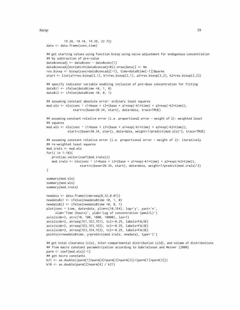
#### example from Gabrielsson and Weiner (2000, page 743)#### endogenous concentration is assumed to be constant over timedose <- 36630time <- c(-1, 0.167E-01, 0.1167, 0.1670, 0.25, 0.583, 0.8330, 1.083, 1.583, 2.083, 4.083, 8.083,

12, 23.5, 24.25, 26.75, 32)conc <- c(20.34, 3683, 884.7, 481.1, 215.6, 114, 95.8, 87.89, 60.19, 60.17, 34.89, 20.99, 20.54,

biexp 19

19.28, 18.18, 19.39, 22.72)data <- data.frame(conc,time)

## get starting values using function biexp using naive adjustment for endogenous concentration## by subtraction of pre-valuedata$concadj <- data$conc - data$conc[1]data$concadj[min(which(data$concadj<0)):nrow(data)] <- NAres.biexp <- biexp(conc=data$concadj[-1], time=data$time[-1])$parmsstart <- list(a1=res.biexp[3,1], k1=res.biexp[2,1], a2=res.biexp[3,2], k2=res.biexp[2,2])

## specify indicator variable enabling inclusion of pre-dose concentration for fittingdata$i1 <- ifelse(data$time <0, 1, 0)data$i2 <- ifelse(data$time <0, 0, 1)

## assuming constant absolute error: ordinary least squaresmod.ols <- nls(conc ~ i1*base + i2*(base + a1*exp(-k1*time) + a2*exp(-k2*time)),

start=c(base=20.34, start), data=data, trace=TRUE)

## assuming constant relative error (i.e. proportional error - weight of 2): weighted least## squaresmod.wls <- nls(conc ~ i1*base + i2*(base + a1*exp(-k1*time) + a2*exp(-k2*time)),

start=c(base=20.34, start), data=data, weight=1/predict(mod.ols)^2, trace=TRUE)

## assuming constant relative error (i.e. proportional error - weight of 2): iteratively## re-weighted least squaresmod.irwls <- mod.wlsfor(i in 1:10){

print(as.vector(coef(mod.irwls)))mod.irwls <- nls(conc ~ i1*base + i2*(base + a1*exp(-k1*time) + a2*exp(-k2*time)),

start=c(base=20.34, start), data=data, weight=1/predict(mod.irwls)^2)}

summary(mod.ols)summary(mod.wls)summary(mod.irwls)

newdata <- data.frame(time=seq(0,32,0.01))newdata$i1 <- ifelse(newdata$time <0, 1, 0)newdata$i2 <- ifelse(newdata$time <0, 0, 1)plot(conc ~ time, data=data, ylim=c(10,1E4), log='y', yaxt='n',

xlab='Time (hours)', ylab='Log of concentration (pmol/L)')axis(side=2, at=c(10, 100, 1000, 10000), las=1)axis(side=2, at=seq(1E1,1E2,1E1), tcl=-0.25, labels=FALSE)axis(side=2, at=seq(1E2,1E3,1E2), tcl=-0.25, labels=FALSE)axis(side=2, at=seq(1E3,1E4,1E3), tcl=-0.25, labels=FALSE)points(x=newdata$time, y=predict(mod.irwls, newdata), type='l')

## get total clearance (cls), inter-compartmental distribution (cld), and volume of distributions## from macro constant parametrization according to Gabrielsson and Weiner (2000)parm <- coef(mod.wls)[-1]## get micro constantsk21 <- as.double((parm[1]*parm[4]+parm[3]*parm[2])/(parm[1]+parm[3]))k10 <- as.double(parm[2]*parm[4] / k21)

20 biexp

k12 <- as.double(parm[2]+parm[4] - k21 - k10)## get cls, cld, vc, and vtcls <- as.double(dose / (parm[1]/parm[2] + parm[3]/parm[4]))vc <- as.double(dose / (parm[1] + parm[2]))cld <- k12*vcvt <- cld / k21print(c(cls, cld, vc, vt))

## turnover model to account for endogenous baseline according to Gabrielsson and Weiner## using a biexponential (i.e. two-compartment) model parametrized in terms of clearance

## Not run: require(rgenoud)require(deSolve)

k <- 2 # assuming proportional error - weighting in function objfuntinf <- 1/60 # duration of bolus in hoursdata <- subset(data, time>0)

defun <- function(time, y, parms) {rte1 <- ifelse(time <= tinf, dose/tinf, 0)dCptdt1 <- (rte1 + parms["synt"] - parms["cls"]*y[1] - parms["cld"]*y[1] +

parms["cld"]*y[2]) / parms["vc"]dCptdt2 <- (parms["cld"]*y[1] - parms["cld"]*y[2])/parms["vt"]list(c(dCptdt1, dCptdt2))}

modfun <- function(time, synt, cls, cld, vc, vt) {out <- lsoda(y=c(synt/cls, synt/cls), times=c(0, data$time), defun,

parms=c(synt=synt, cls=cls, cld=cld, vc=vc, vt=vt), rtol=1e-5, atol=1e-5)[-1,2]}

objfun <- function(par) {out <- modfun(data$time, par[1], par[2], par[3], par[4], par[5])gift <- which(data$conc != 0 )sum((data$conc[gift]-out[gift])^2 / data$conc[gift]^k)

}

## grid search to get starting values for Nelder-Mead## increase values of pop.size and max.generation to get better starting values## values of 10 are used for illustration purpose onlyoptions(warn = -1) # omit warning when hard maximum limit is hitgen <- genoud(objfun, nvars=5, max=FALSE, pop.size=10, max.generation=10,

starting.value=c(1500, cls, cld, vc, vt), BFGS=FALSE,print.level=1, boundary.enforcement=2,Domains=matrix(c(0,0,0,0,0,1E4,1E3,1E3,1E3,1E3),5,2),MemoryMatrix=TRUE)

options(warn = 0) # set back to default

opt <- optim(gen$par, objfun, method="Nelder-Mead")

trn.wls <- nls(conc ~ modfun(time, synt, cls, cld, vc, vt), data=data,start=list(synt=opt$par[1], cls=opt$par[2], cld=opt$par[3], vc=opt$par[4],

vt=opt$par[5]),

ci 21

trace=TRUE, nls.control(tol=Inf))

summary(trn.wls)

## End(Not run)

ci Function to extract confidence interval(s)

Description

Generic function that extracts the confidence interval(s) of an object of class PK.

Usage

ci(obj, method=NULL)

Arguments

obj An output object of class PK.

method A character string specifying the method of the confidence interval. If NULL(default) all intervals are returned.

Details

Generic function to allow easy extraction of confidence intervals.

Value

A matrix containing confidence interval bounds.

Author(s)

Thomas Jaki

References


See Also

estimator and test

22 CPI975

Examples

# Example from Nedelman et al. (1995)conc <- c(2790, 3280, 4980, 7550, 5500, 6650, 2250, 3220, 213, 636)time <- c(1, 1, 2, 2, 4, 4, 8, 8, 24, 24)

obj <- auc(conc=conc, time=time, method=c("z", "t"), design="ssd")

## all requested ci'sci(obj)

## a specific cici(obj, method="t")

CPI975 Plasma levels of CPI975 in rats following a single oral dose

Description

The CPI975 data frame has 60 rows and 4 columns.

Format

This data frame contains the following columns:

conc a numeric vector giving the measured plasma level (microgram/mL).

time a numeric vector giving the time since administration (hours).

sex a factor indicating the gender of the rat.

dose a numeric vector indicating the dose administred (mg/kg).

Details

Nedelman et al. (1995), Table 2 describes serial sampling design were the plasma levels are mea-sured at 5 time points over 24 hours for 10 rats. The same experiment was repeated with differentoral dosages and gender.

Source


eqv 23

eqv Bioequivalence between AUCs

Description

Confidence intervals for the ratio of independent or dependent area under the concentration versustime curves (AUCs) to the last time point.

Usage

eqv(conc, time, group, dependent=FALSE, method=c("fieller", "z", "boott"),conf.level=0.90, strata=NULL, nsample=1000,design=c("ssd","batch","complete"), data)

eqv.ssd(conc, time, group, dependent=FALSE, method=c("fieller", "z", "boott"),conf.level=0.90, strata=NULL, nsample=1000, data)

eqv.batch(conc, time, group, dependent=FALSE,method=c("fieller", "z", "boott"),conf.level=0.90, nsample=1000, data)

eqv.complete(conc, time, group, dependent=FALSE,method=c("fieller", "z", "boott"),conf.level=0.90, nsample=1000, data)

Arguments



group A grouping variable. For batch designs a list is required, while a vector is ex-pected otherwise.

dependent Logical variable indicating if concentrations are measured on the same subjectsfor both AUCs (default=FALSE).

method A character string specifying the method for calculation of confidence intervals(default=c("fieller", "z", "boott")).

conf.level Confidence level (default=0.90).strata A vector of one strata variable (default=NULL). Only available for method boott

in a serial sampling design.nsample Number of bootstrap iterations for method boott (default=1000).design A character string indicating the type of design used. Possible values are ssd

(the default) for a serial sampling design, batch for a batch design and completefor a complete data design.

data Optional data frame containing variables named as id, conc, time and group.

24 eqv

Details

Calculation of confidence intervals for the ratio of (independent or dependent) AUCs (from 0 to thelast time point) for serial sampling, batch and complete data designs. In a serial sampling designonly one measurement is available per subject, while in a batch design multiple time points aremeasured for each subject. In a complete data design measurements are taken for all subjects at alltime points. The AUC (from 0 to the last time point) is calculated using the linear trapezoidal ruleon the arithmetic means at the different time points.

The estimation for the complete data design is done by treating the complete data design as abatch design with a single batch. This approach, though correct, is often inefficient. A generalimplementation is not provided as the most efficient analysis strongly depends on the context. Theinterested reader is refered to chapter 8 of Cawello (2003) while some examples can be found underauc.complete.

dependent specifies if the AUCs are dependent, that is measured on the same subjects. If FALSE,the intervals are based on the method of Jaki et al. (2009) for the serial sampling design and on Jakiet al. (in press) for the batch design. For dependent AUCs the method of Wolfsegger and Jaki (inpress), which assumes that animals, batches and time points are equal for both AUCs, is used. Notethat the option dependent is not used in serial sampling designs as by definition only one sample isobtained per subject then.

The fieller method is based on Fieller’s theorem (1954) which uses the asymptotic standard errorsof the individual AUCs and a critical value from a t-distribution with Satterthwaite’s approximation(1946) to the degrees of freedom for calculation of confidence intervals. The z method is based onthe limit distribution for the ratio using the critical value from a normal distribution for calculationof confidence intervals.

The boott method uses the asymptotic standard errors of the ratio of two AUCs while the criticalvalue is obtained by the bootstrap-t approach and follows the idea discussed in the context of serialsampling designs in Jaki T. et al. (2009). An equivalent approach is used in batch designs as well.Using boott an additional strata variable for bootstrapping can be specified in serial sampling de-signs.

If data is specified the variable names conc, time and group are required and represent the corre-sponding variables. If design is batch an additional variable id is required to identify the subject.

Value



eqv 25







Note

This is a wrapper function for eqv.complete, eqv.batch and eqv.ssd. The function calculatespoint and interval estimates for the ratio of AUCs (from 0 to the last time point).

Author(s)

Thomas Jaki

References

Cawello W. (2003). Parameters for Compartment-free Pharmacokinetics. Standardisation of StudyDesign, Data Analysis and Reporting. Shaker Verlag, Aachen.

Fieller E. C. (1954). Some problems in interval estimation. Journal of the Royal Statistical Society,Series B, 16:175-185.

Hand D. and Crowder M. (1996). Practical Longitudinal Data Analysis, Chapman and Hall, Lon-don.

Jaki T., Wolfsegger M. J. and Ploner M. (2009). Confidence intervals for ratios of AUCs in the caseof serial sampling: A comparison of seven methods. Pharmaceutical Statistics, 8(1):12-24.

Jaki T., Wolfsegger M. J. and Lawo J-P. (2010). Establishing bioequivalence in complete and in-complete data designs using AUCs. Journal of Biopharmaceutical Statistics, 20(4):803-820.



26 eqv

Satterthwaite F. E. (1946). An approximate distribution of estimates of variance components. Bio-metrics Bulletin, 2:110-114.


Yeh, C. (1990). Estimation and significant tests of area under the curve derived from incompleteblood sampling. ASA Proceedings of the Biopharmaceutical Section, 74-81.

See Also

auc, estimator, ci and test.

Examples

## example of a serial sampling design from Nedelman et al. (1995)data(CPI975)data <- subset(CPI975,dose>=30)

data$concadj <- data$conc / data$dose

# fieller and z-interval for ratio of dose-normalized AUCseqv(conc=data$concadj, time=data$time, group=data$dose, method=c("z","fieller"),

design="ssd")

# bootstrap-t interval for ratio of dose-normalized AUCs stratified for sexset.seed(310578)eqv(conc=data$concadj, time=data$time, group=data$dose, method="boott",

strata=data$sex, nsample=500, design="ssd")

## Example of an independent batch design from Yeh (1990)conc <- list(batch1=c(0,0,0,0,0,0, 4.690,2.070,6.450,0.1,0.852,0.136,

4.690,4.060,6.450,0.531,1.2,0.607),batch2=c(4,1.3,3.2,0.074,0.164,0.267, 6.68,3.83,6.08,0.669,1.21,0.878,

8.13,9.54,6.29,0.923,1.65,1.04),batch3=c(9.360,13,5.48,1.090,1.370,1.430, 5.180,5.180,2.79,0.804,1.47,1.26,

1.060,2.15,0.827,0.217,0.42,0.35))time <- list(batch1=c(rep(0,6),rep(1,6),rep(4,6)),

batch2=c(rep(0.5,6),rep(2,6),rep(6,6)),batch3=c(rep(8,6),rep(12,6),rep(24,6)))

group <- list(batch1=rep(rep(c(1,2),each=3),3), batch2=rep(rep(c(1,2),each=3),3),batch3=rep(rep(c(1,2),each=3),3))

eqv(conc=conc, time=time, group=group, dependent=FALSE, method=c("fieller"),conf.level=0.90, design="batch")

## example of independent batch data with overlapping batches

estimator 27

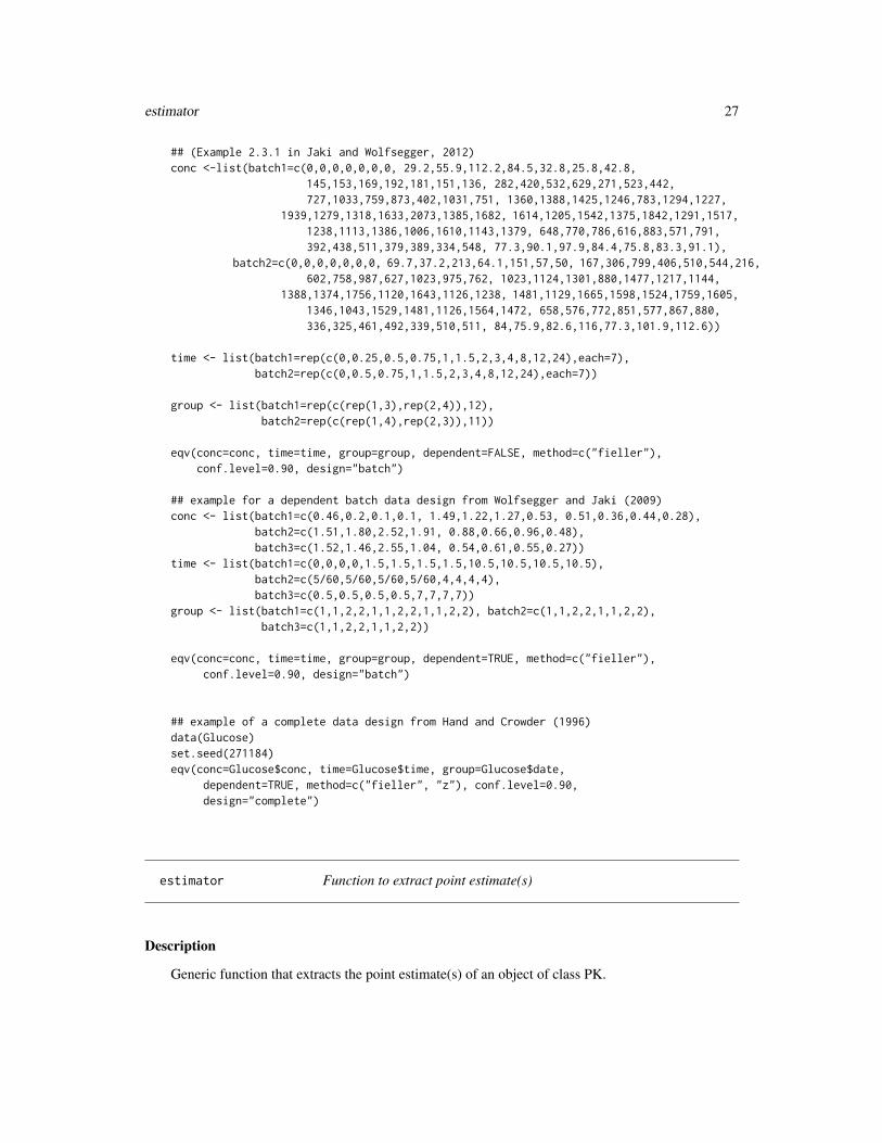
## (Example 2.3.1 in Jaki and Wolfsegger, 2012)conc <-list(batch1=c(0,0,0,0,0,0,0, 29.2,55.9,112.2,84.5,32.8,25.8,42.8,

145,153,169,192,181,151,136, 282,420,532,629,271,523,442,727,1033,759,873,402,1031,751, 1360,1388,1425,1246,783,1294,1227,

1939,1279,1318,1633,2073,1385,1682, 1614,1205,1542,1375,1842,1291,1517,1238,1113,1386,1006,1610,1143,1379, 648,770,786,616,883,571,791,392,438,511,379,389,334,548, 77.3,90.1,97.9,84.4,75.8,83.3,91.1),

batch2=c(0,0,0,0,0,0,0, 69.7,37.2,213,64.1,151,57,50, 167,306,799,406,510,544,216,602,758,987,627,1023,975,762, 1023,1124,1301,880,1477,1217,1144,

1388,1374,1756,1120,1643,1126,1238, 1481,1129,1665,1598,1524,1759,1605,1346,1043,1529,1481,1126,1564,1472, 658,576,772,851,577,867,880,336,325,461,492,339,510,511, 84,75.9,82.6,116,77.3,101.9,112.6))

time <- list(batch1=rep(c(0,0.25,0.5,0.75,1,1.5,2,3,4,8,12,24),each=7),batch2=rep(c(0,0.5,0.75,1,1.5,2,3,4,8,12,24),each=7))

group <- list(batch1=rep(c(rep(1,3),rep(2,4)),12),batch2=rep(c(rep(1,4),rep(2,3)),11))

eqv(conc=conc, time=time, group=group, dependent=FALSE, method=c("fieller"),conf.level=0.90, design="batch")

## example for a dependent batch data design from Wolfsegger and Jaki (2009)conc <- list(batch1=c(0.46,0.2,0.1,0.1, 1.49,1.22,1.27,0.53, 0.51,0.36,0.44,0.28),

batch2=c(1.51,1.80,2.52,1.91, 0.88,0.66,0.96,0.48),batch3=c(1.52,1.46,2.55,1.04, 0.54,0.61,0.55,0.27))

time <- list(batch1=c(0,0,0,0,1.5,1.5,1.5,1.5,10.5,10.5,10.5,10.5),batch2=c(5/60,5/60,5/60,5/60,4,4,4,4),batch3=c(0.5,0.5,0.5,0.5,7,7,7,7))

group <- list(batch1=c(1,1,2,2,1,1,2,2,1,1,2,2), batch2=c(1,1,2,2,1,1,2,2),batch3=c(1,1,2,2,1,1,2,2))

eqv(conc=conc, time=time, group=group, dependent=TRUE, method=c("fieller"),conf.level=0.90, design="batch")

## example of a complete data design from Hand and Crowder (1996)data(Glucose)set.seed(271184)eqv(conc=Glucose$conc, time=Glucose$time, group=Glucose$date,

dependent=TRUE, method=c("fieller", "z"), conf.level=0.90,design="complete")

estimator Function to extract point estimate(s)

Description

Generic function that extracts the point estimate(s) of an object of class PK.

28 estimator

Usage

estimator(obj,se=FALSE)

Arguments


se Logical variable indicating if the standard error should be provided as well (de-fault=FALSE).

Details

Generic function to allow easy extraction of point estimates.

Value

A matrix containing the point estimate(s) and optionally the standard error(s).

Author(s)

Thomas Jaki

References


See Also

ci and test

Examples

# Example from Nedelman et al. (1995)conc <- c(2790, 3280, 4980, 7550, 5500, 6650, 2250, 3220, 213, 636)time <- c(1, 1, 2, 2, 4, 4, 8, 8, 24, 24)

obj <- auc(conc=conc, time=time, method=c('z', 't'), design='ssd')

estimator(obj,TRUE)

Glucose 29

Glucose Baseline adjusted glucose levels following alcohol ingestion

Description

The Glucose data frame has 196 rows and 4 columns. The dataset is originally in package nlme asGlucose2.

Format


id a factor with levels 1 to 7 identifying the subject whose glucose level is measured.date a factor with levels 1 2 indicating the occasion in which the experiment was conducted.time a numeric vector giving the time since alcohol ingestion (in min/10).conc a numeric vector giving the blood glucose level (in mg/dl) adjusted for baseline.

Details

Hand and Crowder (Table A.14, pp. 180-181, 1996) describe data on the blood glucose levelsmeasured at 14 time points over 5 hours for 7 volunteers who took alcohol at time 0. The sameexperiment was repeated on a second date with the same subjects but with a dietary additive usedfor all subjects.

Dataset was corrected for baseline using the following code:

## dataset Glucose2 of package nlmerequire(nlme)Glucose2 <- Glucose2[order(Glucose2$Subject, Glucose2$Date, Glucose2$Time),]## adjust for pre-infusion levels measured at time points -1 and 0data <- NULLfor(i in unique(Glucose2$Subject)){for(j in unique(Glucose2$Date)){

temp <- subset(Glucose2, Subject==i & Date==j)temp$Conc <- temp$glucose - mean(c(temp$glucose[1], temp$glucose[2]))temp$Conc <- ifelse(temp$Conc < 0 | temp$Time <= 0, 0, temp$Conc)## handle intermediate values > 0index1 <- which.max(temp$Conc)index2 <- which.min(temp$Conc[-c(1:index1)]) + index1if(temp$Conc[index2]==0){temp$Conc[c(index2:nrow(temp))] <- 0}data <- rbind(data,temp)

}}Glucose <- subset(data, Time >= 0,

select=c('Subject', 'Date', 'Time', 'Conc'))names(Glucose) <- c("id","date","time","conc")

30 lee

Source

Pinheiro, J. C. and Bates, D. M. (2000), Mixed-Effects Models in S and S-PLUS, Springer, NewYork. (Appendix A.10)

Hand, D. and Crowder, M. (1996), Practical Longitudinal Data Analysis, Chapman and Hall, Lon-don.

lee Two-phase half-life estimation by linear fitting

Description

Estimation of initial and terminal half-life by two-phase linear regression fitting.

Usage

lee(conc, time, points=3, method=c("ols", "lad", "hub", "npr"), lt=TRUE)

Arguments


time Time points of concentration assessment.

points Minimum number of data points in the terminal phase (default=3).

method Method of model fitting (default=ols).

lt Logical value indicating whether requesting a longer terminal than initial half-life (default=TRUE).

Details

Estimation of initial and terminal half-life based on the method of Lee et al. (1990). This methoduses a two-phase linear regression approach separate the model into two straight lines based onthe selection of the log10 transformed concentration values. For two-phase models the initial andterminal half-lives were determined from the slopes of the regression lines. If a single-phase modelis selected by this method, the corresponding half-life is utilized as both initial and terminal phasehalf-life. Half-life is determined only for decreasing initial and terminal phases.

The method ols uses the ordinary least squares regression (OLS) to fit regression lines.

The method lad uses the absolute deviation regression (LAD) to fit regression lines by using the al-gorithm as described in Birkes and Dodge (chapter 4, 1993) for calculation of regression estimates.

The method hub uses the Huber M regression to fit regression lines. Huber M-estimates are cal-culated by non-linear estimation using the function optim, where OLS regression parameters are

lee 31

used as starting values. The function that is minimized involved k = 1.5*1.483*MAD, where MADis defined as the median of absolute deviation of residuals obtained by a least absolute deviation(LAD) regression based on the observed data. The initial value of MAD is used and not updatedduring iterations (Holland and Welsch, 1977).

The method npr uses the nonparametric regression to fit regression lines by using the algorithm asdescribed in Birkes and Dodge (chapter 6, 1993) for calculation of regression estimates.

The selection criteria for the best tuple of regression lines is the sum of squared residuals for theols method, the sum of Huber M residuals for the hub method, the sum of absolute residuals forthe lad method and the sum of a function on ranked residuals for the npr method (see Birkes andDodge (page 115, 1993)). Calculation details can be found in Wolfsegger (2006).

When lt=TRUE, the best two-phase model where terminal half-life >= initial half-life >= 0 is se-lected. When lt=FALSE, the best two-phase model among all possible tuples of regression is se-lected which can result in longer initial half-life than terminal half-life and/or in half-lifes < 0.

Value

A list of S3 class "halflife" containing the following components:

parms half-life and model estimates.

chgpt change point between initial and terminal phase.

time time points of concentration assessments.

conc levels of concentrations.

method "lee".

Note

Records including missing values and concentration values below or equal to zero are omitted.

Author(s)

Martin J. Wolfsegger

References

Birkes D. and Dodge Y. (1993). Alternative Methods of Regression. Wiley, New York, Chichester,Brisbane, Toronto, Singapore.

32 lee

Gabrielsson J. and Weiner D. (2000). Pharmacokinetic and Pharmacodynamic Data Analysis:Concepts and Applications. 4th Edition. Swedish Pharmaceutical Press, Stockholm.

Holland P. W. and Welsch R. E. (1977). Robust regression using iteratively reweighted least-squares. Commun. Statist.-Theor. Meth. A6(9):813-827.

Lee M. L., Poon Wai-Yin, Kingdon H. S. (1990). A two-phase linear regression model for biologichalf-life data. Journal of Laboratory and Clinical Medicine. 115(6):745-748.

Wolfsegger M. J. (2006). The R Package PK for Basic Pharmacokinetics. Biometrie und Medizin,5:61-68.

Examples

#### example for preparation 1 from Lee et al. (1990)time <- c(0.5, 1.0, 4.0, 8.0, 12.0, 24.0)conc <- c(75, 72, 61, 54, 36, 6)res1 <- lee(conc=conc, time=time, method='ols', points=2, lt=TRUE)res2 <- lee(conc=conc, time=time, method='ols', points=2, lt=FALSE)plot(res1, log='y', ylim=c(1,100))plot(res2, add=TRUE, lty=2)

#### example for preparation 2 from Lee et al. (1990)time <- c(0.5, 1.0, 2.0, 6.5, 8.0, 12.5, 24.0)conc <- c(75, 55, 48, 51, 39, 9, 5)res3 <- lee(conc=conc, time=time, method='ols', points=2, lt=FALSE)print(res3$parms)plot(res2, log='y', ylim=c(1,100), lty=1, pch=20)plot(res3, add=TRUE, lty=2, pch=21)legend(x=0, y=10, pch=c(20,21), lty=c(1,2), legend=c('Preperation 1','Preperation 2'))

#### artificial exampletime <- seq(1:10)conc <- c(1,2,3,4,5,5,4,3,2,1)res4 <- lee(conc=conc, time=time, method='lad', points=2, lt=FALSE)plot(res4, log='y', ylim=c(1,7), main='', xlab='', ylab='', pch=19)

#### dataset Indometh of package datasetsrequire(datasets)res5 <- data.frame(matrix(ncol=3, nrow=length(unique(Indometh$Subject))))colnames(res5) <- c('ID', 'initial', 'terminal')row <- 1for(i in unique(Indometh$Subject)){

temp <- subset(Indometh, Subject==i)res5[row, 1] <- unique(temp$Subject)res5[row, c(2:3)] <- lee(conc=temp$conc, time=temp$time, method='lad')$parms[1,]row <- row + 1

nca 33

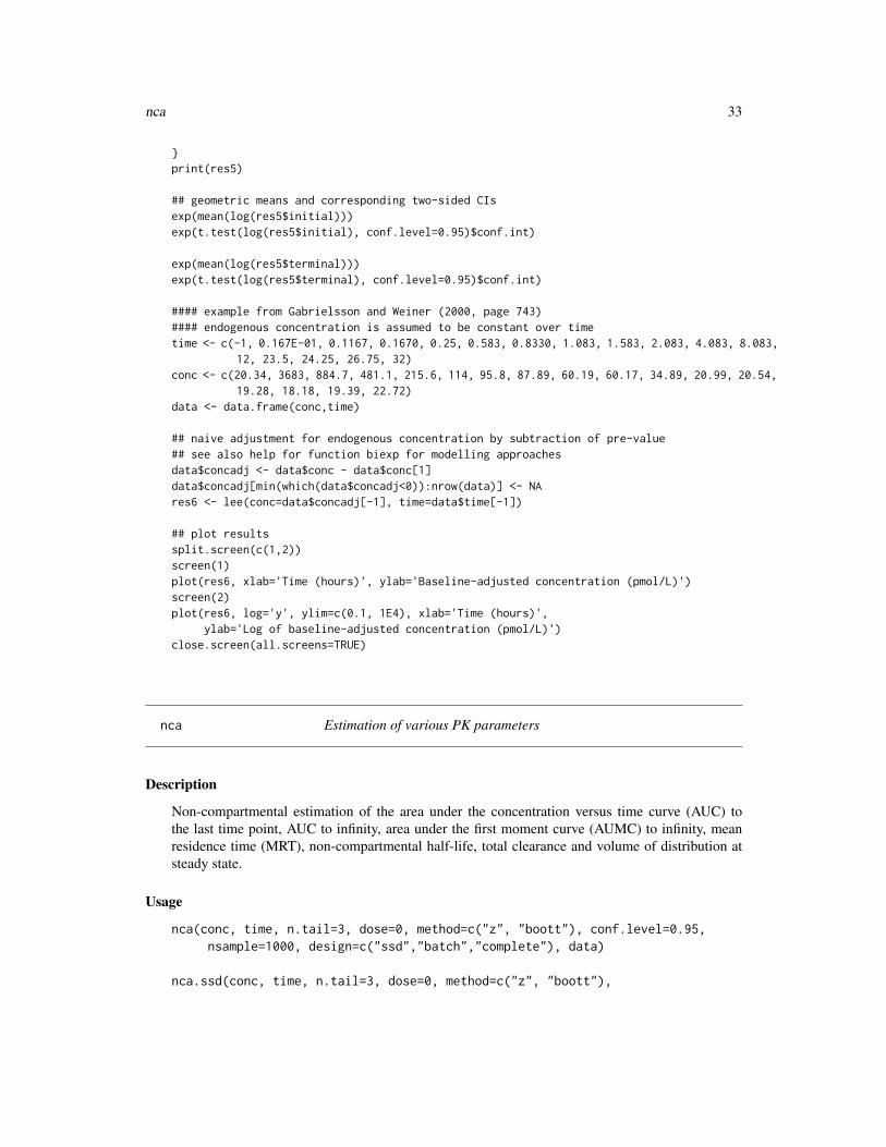
}print(res5)

## geometric means and corresponding two-sided CIsexp(mean(log(res5$initial)))exp(t.test(log(res5$initial), conf.level=0.95)$conf.int)

exp(mean(log(res5$terminal)))exp(t.test(log(res5$terminal), conf.level=0.95)$conf.int)

#### example from Gabrielsson and Weiner (2000, page 743)#### endogenous concentration is assumed to be constant over timetime <- c(-1, 0.167E-01, 0.1167, 0.1670, 0.25, 0.583, 0.8330, 1.083, 1.583, 2.083, 4.083, 8.083,

12, 23.5, 24.25, 26.75, 32)conc <- c(20.34, 3683, 884.7, 481.1, 215.6, 114, 95.8, 87.89, 60.19, 60.17, 34.89, 20.99, 20.54,

19.28, 18.18, 19.39, 22.72)data <- data.frame(conc,time)

## naive adjustment for endogenous concentration by subtraction of pre-value## see also help for function biexp for modelling approachesdata$concadj <- data$conc - data$conc[1]data$concadj[min(which(data$concadj<0)):nrow(data)] <- NAres6 <- lee(conc=data$concadj[-1], time=data$time[-1])

## plot resultssplit.screen(c(1,2))screen(1)plot(res6, xlab='Time (hours)', ylab='Baseline-adjusted concentration (pmol/L)')screen(2)plot(res6, log='y', ylim=c(0.1, 1E4), xlab='Time (hours)',

ylab='Log of baseline-adjusted concentration (pmol/L)')close.screen(all.screens=TRUE)

nca Estimation of various PK parameters

Description

Non-compartmental estimation of the area under the concentration versus time curve (AUC) tothe last time point, AUC to infinity, area under the first moment curve (AUMC) to infinity, meanresidence time (MRT), non-compartmental half-life, total clearance and volume of distribution atsteady state.

Usage

nca(conc, time, n.tail=3, dose=0, method=c("z", "boott"), conf.level=0.95,nsample=1000, design=c("ssd","batch","complete"), data)

nca.ssd(conc, time, n.tail=3, dose=0, method=c("z", "boott"),

34 nca

conf.level=0.95, nsample=1000, data)

nca.batch(conc, time, n.tail=3, dose=0, method=c("z", "boott"),conf.level=0.95, nsample=1000, data)

nca.complete(conc, time, n.tail=3, dose=0, method=c("z", "boott"),conf.level=0.95, nsample=1000, data)

Arguments



n.tail Number of last data points used for tail area correction (default=3).

dose Dose administered as an IV bolus (default=0).

method A character string specifying the method for calculation of confidence intervals(default=c("z", "boott")).


nsample Number of bootstrap iterations for bootstrap-t interval (default=1000).

design A character string indicating the type of design used. Possible values are ssd(the default) for a serial sampling design, batch for a batch design and completefor a complete data design.

data Optional data frame containing variables named as id, conc and time.

Details

Estimation of the area under the concentration versus time curve from zero to the last time point(AUC 0-tlast), total area under the concentration versus time curve from zero to infinity (AUC0-Inf), area under the first moment curve for zero to infinity (AUMC 0-Inf), mean residence time(MRT), non-compartmental half-life (HL), total clearance (CL) and volume of distribution at steadystate (Vss). In a serial sampling design only one measurement is available per subject at a specifictime point, while in a batch design multiple time points are measured for each subject. In a com-plete data design measurements are taken for all subjects at all time points.

A constant coefficient of variation at the last n.tail time points is assumed.

The use of the standard errors and confidence intervals for the MRT and Vss from batch designsis depreciated due to very slow asymptotic that usually lead to severe undercoverage. For com-plete data designs only point estimates are provided. The parameters method, conf.level andnsample=1000 are therefore not used. If data for only one subject is provided, the parameters areestimated for this subject while the geometric mean of the estimated parameters is found for multi-ple subjects (see Cawello, 2003, p. 114).

nca 35

The AUC 0-tlast is calculated using the linear trapezoidal rule on the arithmetic means at the differ-ent time points while the extrapolation necessary for the AUC 0-Inf and AUMC 0-Inf is achievedassuming an exponential decay on the last n.tail time points. The other parameters are functionsof these PK parameters and of the dosage and are defined as in Wolfsegger and Jaki (2009).

Two different confidence intervals are computed: an asymptotic confidence interval and a bootstrap-t interval. The z method is based on the limit distribution of the parameter using the critical valuefrom a normal distribution for calculation of confidence intervals together with asymptotic vari-ances. The bootstrap-t interval uses the same asymptotic variances, but while the critical value isobtained by the bootstrap-t approach. If nsample=0 only the asymptotic interval will be computed.

If data is specified the variable names conc and time are required and represent the correspondingvariables.

Note that some estimators as provided assume IV bolus administration. If an oral administration isused- The clearance needs to be adjusted by the bioavailability, f. This can be achieved by either multi-plying the obtained estimator by f or adjusting the dose parameter accordingly.- The MRT estimate produced corresponds to the mean transit time (MTT) which is the sum ofMRT and mean absorption time (MAT).- HL and Vss are functions of the MRT and hence they will not be valid under oral administration.

Value








Note

At present only the option serial sampling design is available.

Author(s)


36 nca

References

Cawello W. (2003). Parameters for compartment-free pharmacokinetics. Standardisation of studydesign, data analysis and reporting. Shaker Verlag, Aachen.



Wolfsegger M. J. and Jaki T. (2009). Non-compartmental Estimation of Pharmacokinetic Parame-ters in Serial Sampling Designs. Journal of Pharmacokinetics and Pharmacodynamics, 36(5):479-494.

See Also

auc, estimator, ci and test.

Examples

#### serial sampling designs## example for a serial sampling data design from Wolfsegger and Jaki (2009)conc <- c(0, 0, 0, 2.01, 2.85, 2.43, 0.85, 1.00, 0.91, 0.46, 0.35, 0.63, 0.39, 0.32,

0.45, 0.11, 0.18, 0.19, 0.08, 0.09, 0.06)time <- c(rep(0,3), rep(5/60,3), rep(3,3), rep(6,3), rep(9,3), rep(16,3), rep(24,3))

# Direct call of the function# CAUTION: this might take a few minutes# Note: 1E4 bootstrap replications were used in the example given# in Wolfsegger and Jaki (2009)set.seed(34534)nca.ssd(conc=conc, time=time, n.tail=4, dose=200, method=c("z","boott"),

conf.level=0.95, nsample=500)

# Call through the wrapper function using datadata <- data.frame(conc=conc, time=time)nca(data=data, n.tail=4, dose=200, method="z",

conf.level=0.95, design="ssd")

#### batch design:## a batch design example from Holder et al. (1999).data(Rats)data <- subset(Rats,Rats$dose==100)

# using the wrapper function

PKNews 37

nca(data=data, n.tail=4, dose=100, method="z",conf.level=0.95, design="batch")

# direct callnca.batch(data=data, n.tail=4, dose=100, method="z",

conf.level=0.95)

## example with overlapping batches (Treatment A in Example of Jaki & Wolfsegger 2012)conc <- list(batch1=c(0,0,0,0, 69.7,37.2,213,64.1, 167,306,799,406, 602,758,987,627,

1023,1124,1301,880, 1388,1374,1756,1120, 1481,1129,1665,1598,1346,1043,1529,1481, 658,576,772,851, 336,325,461,492,84,75.9,82.6,116),

batch2=c(0,0,0, 29.2,55.9,112.2, 145,153,169, 282,420,532, 727,1033,759,1360,1388,1425, 1939,1279,1318, 1614,1205,1542, 1238,1113,1386,648,770,786, 392,438,511, 77.3,90.1,97.9))

time <- list(batch1=rep(c(0,0.5,0.75,1,1.5,2,3,4,8,12,24),each=4),batch2=rep(c(0,0.25,0.5,0.75,1,1.5,2,3,4,8,12,24),each=3))

nca.batch(conc,time,method="z",n.tail=4,dose=80)

#### complete data design## example from Gibaldi and Perrier (1982, page 436) for individual PK parameterstime <- c(0, 0.165, 0.5, 1, 1.5, 3, 5, 7.5, 10)conc <- c(0, 65.03, 28.69, 10.04, 4.93, 2.29, 1.36, 0.71, 0.38)# using the wrapper functionnca(conc=conc, time=time, n.tail=3, dose=1E6, design="complete")# direct callnca.complete(conc=conc, time=time, n.tail=3, dose=1E6)

PKNews Shows changes and news

Description

Functions showing changes since previous versions.

Usage

PKNews()

Details

Displays the changes and news given in the NEWS file of the package.

Value

Screen output.

Author(s)

Thomas Jaki

38 plot.halflife

Examples

PKNews()

plot.halflife Plot regression lines used for half-life estimation

Description

This method plots objects of S3 class "halflife" (biexp and lee).

Usage

## S3 method for class 'halflife'plot(x, xlab='Time', ylab='Concentration',

main='Half-life Estimation', xlim=NULL, ylim=NULL, add=FALSE, ...)

Arguments

x An object of S3 class "halflife" (biexp and lee).

xlab A label for the x axis.

ylab A label for the y axis.

main A main title for the plot.

xlim The x limits (min, max) of the plot.

ylim The y limits (min, max) of the plot.

add A logical value indicating whether to add plot to current plot (default=FALSE).

... Other parameters to be passed through to plotting functions.

Value

none

Author(s)

Martin J. Wolfsegger

Rats 39

Rats Plasma levels in female rats following a single oral dose

Description

The Rats data frame has 126 rows and 4 columns.

Format


id a numeric vector identifying the animal whose plasma level is measured.

conc a numeric vector giving the measured plasma level (microgram/mL).


dose a numeric vector indicating the dose administred (mg/kg).

Details

Holder et al. (1999), Table 4 describes data on the plasma levels measured at 6 time points over 24hours for 9 female rats. The same experiment was repeated with different oral dosages.

Source


Rep.tox Plasma levels in rats following daily intravenous administration in arepeated dose toxicity study

Description

The Rep.tox data frame has 28 rows and 4 columns and gives the plasma levels of 6 rats in arepeated dose toxicity study.

Format


id a numeric vector identifying the animal whose plasma level is measured.

conc a numeric vector giving the measured plasma level (IU/mL).


day a numeric vector indicating the day the data were collected.

40 test

Details

In this study the compound is administered daily to 6 Rats over 14 days. Plasma levels are measuredat 7 time points over 12 hours after the first administration and after the 14th administration.

Source


test Function for hypothesis testing for objects of class PK

Description

Generic function for hypothesis testing based on an object of class PK.

Usage

test(obj, theta=0, method = c("t", "fieller", "z", "resample"), nsample = 1000)

## S3 method for class 'PKtest'print(x,hyp=FALSE,...)

## S3 method for class 'PKtest'summary(object,...)

Arguments


x An output object of class PKtest.

object An output object of class PK test.

theta The reference value to be tested against. If multiple parameters are to be testeda vector can be supplied.

method A character string specifying the method for calculation of the test statistic. Pos-sible values are t (the default) and fieller for a t-test based method, z for az-test and resample for either a bootstrap or a permutation test.

nsample Number of resamples for the permutation/bootstrap test (default=1000).

hyp Logical variable indicating if hypothesis tests should be printed explicitly (de-fault=FALSE).

... Arguments to be passed to methods, such as graphical.

test 41

Details

Generic function to perform hypothesis test(s).

The reference value for the test is to be specified in theta. If multiple tests are performed theta canbe a vector.

For method "resample" a permutation test is used for the difference of AUCs while a one-samplebootstrap test based on inverting a bootstrap-t statistic is implemented.

Value

An object of the class PKtest containing the following components:

stat Test statistics.

p.value p-values.

theta Reference value(s) tested against.


alternative Type of alternative used.

df Degrees of freedom of method "t".


method Type of test used.

Author(s)

Thomas Jaki

References

Efron B and Tibshirani R. J. (1993). An introduction to the bootstrap, Chapman and Hall, NewYork.



42 test

See Also

auc, eqv and nca.

Examples

## example for a serial sampling data design from Wolfsegger and Jaki (2009)conc <- c(0, 0, 0, 2.01, 2.85, 2.43, 0.85, 1.00, 0.91, 0.46, 0.35, 0.63, 0.39, 0.32,

0.45, 0.11, 0.18, 0.19, 0.08, 0.09, 0.06)time <- c(rep(0,3), rep(5/60,3), rep(3,3), rep(6,3), rep(9,3), rep(16,3), rep(24,3))

obj <- nca(conc=conc, time=time, n.tail=4, dose=200, method="z",conf.level=0.95, design="ssd")

## testing all parameters against different values using a z-testres <- test(obj, theta=c(11, 12, 90, 7, 5, 16, 120), method="z")

print(res)

## a batch design example from Holder et al. (1999).data(Rats)data <- subset(Rats,Rats$dose==100)

obj <- auc(data=data,method=c('z','t'), design='batch')

## t-testres <- test(obj, theta=100, method="t")

## making the hypothesis explicitsummary(res)

## bootstrap test for bioequivalence# Note: This can take a few secondsdata(Glucose)## one-sided permutation testobj <- auc(conc=Glucose$conc, time=Glucose$time, group=Glucose$date,

method=c("t"), conf.level=0.90, alternative='less',nsample=100, design="complete")

test(obj, theta=1, method="resample", nsample=100)

Index

∗Topic classesall.class, 2

∗Topic datasetsCPI975, 22Glucose, 29Rats, 39Rep.tox, 39

∗Topic hplotplot.halflife, 38

∗Topic htestauc, 5auc.complete, 12eqv, 23nca, 33test, 40

∗Topic manipci, 21estimator, 27

∗Topic miscbiexp, 15lee, 30PKNews, 37

all.class, 2auc, 5, 12, 13, 26, 36, 42auc.batch, 7auc.complete, 7, 8, 11, 24auc.ssd, 7

biexp, 15, 38

ci, 3, 8, 13, 21, 26, 28, 36CPI975, 22

eqv, 8, 23, 42eqv.batch, 25eqv.complete, 25eqv.ssd, 25estimator, 3, 8, 13, 21, 26, 27, 36

Glucose, 29

lee, 16, 30, 38

nca, 8, 33, 42

PKNews, 37plot.halflife, 38plot.PK (all.class), 2print.PK (all.class), 2print.PKtest (test), 40

Rats, 39Rep.tox, 39

summary.PK (all.class), 2summary.PKtest (test), 40

test, 3, 8, 13, 21, 26, 28, 36, 40

43

package ‘pk’ - r · package ‘pk ’ february 26, 2018 ... description estimation of...

Documents