NBER WORKING PAPER SERIES

PARENTAL INCENTIVES AND EARLY CHILDHOOD ACHIEVEMENT:A FIELD EXPERIMENT IN CHICAGO HEIGHTS

Roland G. Fryer, Jr.Steven D. Levitt

John A. List

Working Paper 21477http://www.nber.org/papers/w21477

NATIONAL BUREAU OF ECONOMIC RESEARCH1050 Massachusetts Avenue

Cambridge, MA 02138August 2015

Special thanks to the Griffin Foundation for funding this research. Also, Tom Amadio, Superintendentof Chicago Heights, was a superb partner through his leadership and support during this project. TanayaDevi, Rucha Vankudre, Anya Samek, Eric Anderson, Martha Woerner, and Sara D’Alessandro providedexceptional research assistance and project management support. The views expressed herein are thoseof the authors and do not necessarily reflect the views of the National Bureau of Economic Research.

NBER working papers are circulated for discussion and comment purposes. They have not been peer-reviewed or been subject to the review by the NBER Board of Directors that accompanies officialNBER publications.

© 2015 by Roland G. Fryer, Jr., Steven D. Levitt, and John A. List. All rights reserved. Short sectionsof text, not to exceed two paragraphs, may be quoted without explicit permission provided that fullcredit, including © notice, is given to the source.

Parental Incentives and Early Childhood Achievement: A Field Experiment in Chicago HeightsRoland G. Fryer, Jr., Steven D. Levitt, and John A. ListNBER Working Paper No. 21477August 2015JEL No. I20,J01

ABSTRACT

This article describes a randomized field experiment in which parents were provided financial incentivesto engage in behaviors designed to increase early childhood cognitive and executive function skillsthrough a parent academy. Parents were rewarded for attendance at early childhood sessions, completinghomework assignments with their children, and for their child’s demonstration of mastery on interimassessments. This intervention had large and statistically significant positive impacts on both cognitiveand non-cognitive test scores of Hispanics and Whites, but no impact on Blacks. These differentialoutcomes across races are not attributable to differences in observable characteristics (e.g. family size,mother’s age, mother’s education) or to the intensity of engagement with the program. Children withabove median (pre-treatment) non cognitive scores accrue the most benefits from treatment.

Roland G. Fryer, Jr.Department of EconomicsHarvard UniversityLittauer Center 208Cambridge, MA 02138and NBERrfryer@fas.harvard.edu

Steven D. LevittDepartment of EconomicsUniversity of Chicago1126 East 59th StreetChicago, IL 60637and NBERslevitt@midway.uchicago.edu

John A. ListDepartment of EconomicsUniversity of Chicago1126 East 59thChicago, IL 60637and NBERjlist@uchicago.edu

There is no program or policy that can substitute for a mother or father who will attend those parent-teacher

conferences or help with the homework or turn off the TV, put away the video games, read to their child.

Responsibility for our children’s education must begin at home.

--Barack Obama in an address to a Joint Session of Congress 2009

Parental inputs matter. Children quasi-randomly assigned via adoption to highly

educated parents and small families are twice as likely to graduate from a college ranked by

U.S. News & World Report, have an additional .75 years of schooling, and are 16 percent

more likely to complete four years of college (Sacerdote 2007). Black et al (2005)

demonstrate that birth order has an important impact on educational attainment, adult

earnings, employment, and teenage childbearing. Many believe that the importance of

parental inputs – along with the racial and income differences that exists in such inputs – is

an important cause of intergenerational inequality (Becker and Tomes 1979).1

In an effort to increase the quantity and quality of early life experiences and decrease

the gaps between race and income groups in these formative years, early education programs

have become laboratories of reform.2 One potentially cost-effective – and scalable – strategy,

not yet tested in America, is providing short-term financial incentives for parents to increase

their involvement with their children or exhibit certain behaviors believed to be important

for the production of human capital. Theoretically, providing such incentives could have one

of three possible effects. First, if low-income parents lack sufficient motivation, heavily

discount the future, or lack accurate information on either the educational production

function or the returns to parental investment, providing incentives for parental involvement

will yield increases in parental participation and potentially child achievement. Second, if

parents lack structural resources to convert effort to output, or the production function of

child achievement has important complementarities out of their control (e.g. adequate food

1 There are large racial and income differences in parental inputs. Black children are reared in environments with 58% less books than whites and are less likely to engage in activities such as going to museums (Fryer and Levitt 2004). From birth to kindergarten entry, black children spend 1,300 less hours in conversations with adults than white children (Phillips 2011). Hart and Risley (1995) argue that children from low-income families hear 30 million fewer words than children from high-income families. 2 There is a large established literature on the efficacy of early childhood interventions. The evidence on the scalability of these strategies -- due to cost, access, and replicability of results – is less clear. See Almond and Currie (2010) for an extensive review of the literature. York and Loeb (2014) provide new evidence on the positive effects of a text messaging program for preschoolers designed to help them facilitate literacy development.

1

supply, safe neighborhoods, or health care), then incentives will have little impact. Third,

some argue that financial rewards (or any type of external reward or incentive) crowd out

intrinsic motivation and lead to negative outcomes in the long run. Which one of the above

effects – investment incentives, structural inequalities, or intrinsic motivation – will dominate

is unknown. The experimental estimates obtained in this study will combine elements from

these and other potential channels.

In the 2011-2012 school year, we conducted a parental incentive experiment in

Chicago Heights – a prototypical low performing urban school district – by starting a parent

academy that distributed nearly $1 million to 257 families (figures include treatment and

control).3 There were two treatment groups, which differed only in when families were

rewarded, and a control group. Parents in the two treatment groups were paid for attendance

at Parent Academy sessions, proof of homework completion, and the performance of their

children on benchmark assessments. The only difference between the two treatment groups

is that parents in one group were paid in cash or via direct deposits (hereafter the “cash”

condition) and parents in the second group received the majority of their incentive payments

via deposits into a trust account which can only be accessed if and when the child enrolls in

college (the “college” incentive condition). Eleven project managers and staff worked

together to ensure that parents understood the particulars of the treatment; that the parent

academy program was implemented with high fidelity; and that payments were distributed

on-time and accurately.

Across the entire sample, the impact on cognitive test scores of being offered a

chance to participate in our parental incentive is 0.119σ (with a standard error of 0.094).4

These estimates are non-trivial, but smaller in magnitude than some classroom based

interventions. For instance, the impact of Head Start on test scores is approximately 0.145σ.

The impact of the Perry Preschool intervention on achievement at 14 years old is 0.203σ.

Given the imprecision of the estimates, however, our results are statistically indistinguishable

3 In 2010, we conducted a pilot experiment designed to work out operational and logistical challenges and to write a year-long curriculum. Results from the pilot are provided in Appendix Tables 10-14. 4 An important limitation of our field experiment is that it was constructed to detect treatment effects of 0.2 standard deviations or more with eighty percent power. Thus, we are underpowered to estimate effect sizes below this cutoff, many of which could have a positive return on investment. This level of power seemed reasonable ex ante given the relatively large effect sizes reported in the early childhood literature (see, e.g., Zaslow et al. 2010).

2

both from these programs and from zero. The impact of the “college” and “cash” incentive

schemes are nearly identical.

The impact of being offered a chance to participate in our parental incentive scheme

on non-cognitive skills is large and statistically significant (0.203σ (0.083)). These results are

consistent with Kautz et al. (2014), who argue that parental investment is an important

contributor to non-cognitive development. Again, the “cash” and “college” schemes yield

identical results.

We complement our main statistical analysis by estimating heterogeneous treatment

effects across a variety of pre-determined subsamples that we blocked on experimentally.

Two stark patterns appear in the data. The first pattern is along racial lines: Hispanics (48

percent of our sample) and Whites (8 percent of the sample) demonstrate large and

significant increases in both cognitive and non-cognitive domains. For instance, the impact

of our parent academy for Hispanic children is 0.367σ (0.133) on our cognitive score and

0.428σ (0.122) on our non-cognitive score. Among the small sample of Whites, the impacts

are 0.932σ (0.353) on cognitive and 0.821σ (0.181) on non-cognitive. The identical estimates

for Blacks are actually negative but statistically insignificant on both cognitive and non-

cognitive dimensions: -0.234σ (0.134) and -0.059σ (0.129), respectively. Importantly, p-

values on the differences across races are statistically significant at conventional levels.5 We

explore a range of possible hypotheses regarding the source of the racial differences (extent

of engagement with the program, demographics, English proficiency, pre-treatment scores),

but none provide a convincing explanation of the complete effect.

The second pattern of heterogeneity in treatment that we observe in the data relates

to pre-treatment test scores. Students who enter our program below the median on non-

cognitive skills see no benefits from our intervention in either the cognitive or non-cognitive

domain. In stark contrast, students who enter our parent academy above the median in non-

cognitive skills experience treatment effects of roughly 0.3 standard deviations on both

5 This pattern of racial heterogeneity is a recurring theme in the literature on early childhood achievement. Gentzkow and Shapiro (2008) demonstrate that an additional year of preschool television has marginally significant positive effects on reading and general knowledge scores. However, these effects are the largest for children from households where the primary language is not English and for non-white children. Currie and Thomas (1999) report that Head Start pre-school closes at least one-fourth of the gap in test scores between Latino children and non-Hispanic white children, and two-thirds of the gap in the probability of grade repetition. The Parents as Teachers program, which is a parent education program that is designed to strengthen parent’s knowledge of child development and help prepare their children for school, has larger effects on Latino families than on non-Latino families (Wagner and Clayton 1999).

3

cognitive and non-cognitive dimensions. If we segment children by both cognitive and non-

cognitive pre-treatment scores, the greatest gains are made on both the cognitive and non-

cognitive dimension by students who start the program above the median on non-cognitive

skills and below the median on cognitive skills. A similar complementary between cognitive

and non-cognitive skills has been observed in observational studies (Weinberger 2014).

The remainder of our paper is structured as follows. Section II gives a brief review of

the experimental literature on parental incentives. Section III provides some details of our

experiment and its implementation. Section IV details the data, research design, and

estimating equations used in our analysis. Section V presents estimates of the impact of

parental incentives on a child’s cognitive and non-cognitive skills. Section VI provides some

discussion and speculation about potential theories that might explain the differences

between racial groups in estimated treatment effects. There are two online appendices.

Appendix A is an implementation supplement that provides details on the timing of our

experimental roll-out and critical milestones reached. Appendix B is a data appendix that

provides details on how we construct our covariates and our samples from the data collected

for the purposes of this study.

II. A Brief Literature Review on Parental Incentives for Achievement

This paper lies at the intersection of several literatures: (1) early childhood

interventions such as Perry Pre-School or Head Start; (2) parental education interventions

such as Parents as Teachers; and (3) a small literature on parental incentives. An extensive

review of the first of these literatures is provided by Almond and Currie (2010). Likewise,

Nye et al. (2006) provide a systematic review of the second literature. Interested readers are

directed to those studies for excellent work in these two areas. We are not aware of a

parallel survey on the emerging literature on parental incentives to increase educational

achievement (e.g. Fryer 2011, Middleton et al. 2005, Skoufias 2005, Attanasio et al. 2005,

Chaudhury and Parajuli 2006 and Kremer, Miguel and Thornton 2009).

The most well-known and well analyzed incentive program for parents is

PROGRESA, which was an experiment conducted in Mexico in 1998 that provided cash

incentives linked to health, nutrition, and education. The largest component of PROGRESA

was linked to school attendance and enrollment. The program provided cash payments to

mothers in targeted households to keep their children in school (Skoufias 2005). As a part of

4

the program, households could receive up to $62.50 per month if children attended school

regularly. The average amount of incentives received by treatment households in the first

two years of treatment was $34.80, which was 21% of an average household’s income.

Besides school attendance, PROGRESA also emphasized actual student achievement by

making a child ineligible for the program if she failed a grade more than once (Skoufias 2005,

Slavin et al. 2009).

Schultz (2000) reports that PROGRESA had a positive impact on school enrollment

for both boys and girls in primary and secondary school. For primary school children,

PROGRESA increased school enrollment for boys by 1.1 percentage points and 1.5

percentage points for girls from a baseline level of approximately 90 percent. For secondary

school students, enrollment increased by 7.2 to 9.3 percentage points for boys and 3.5 to 5.8

percentage points for girls, from a baseline level of approximately 70%. The author also

reports that PROGRESA had an accumulated effect of 0.66 years additional schooling for a

student from the average poor household. Taking the baseline level of schooling at face

value, PROGRESA’s 0.66 years accumulated effect translates into a 10% increase in

schooling attainment.6

Opportunity NYC – modeled after PROGRESA – was an experimental conditional

cash transfer program that was conducted in New York City. The program had three

components: the Family Rewards component that gave incentives to parents to fulfill

responsibilities towards their children; the Work Rewards component that gave incentives

for families to work; and the Spark component that gave student incentives to increase

achievement scores in classes. The program began in August 2007 and ended in August 2010

(Silva 2008).

Riccio et al. (2013) analyze data from the Family Rewards component of the program

during the first two years of treatment. Their analysis is based on 4,800 families with 11,000

children out of which half were assigned to treatment and the other half to control.

Opportunity NYC spent $8,700 per family in treatment over three years. The program had

an insignificant impact on school outcomes (Riccio et al. 2013). The children’s award

6 Behrman, Sengupta, and Todd (2001) also analyze the data and report that PROGRESA children entered school at an earlier age, had less grade repetition, and better grade progression. Treatment children also had lower dropout rates and once dropped out, they had a higher chance of re-entry into high school.

5

experiment, analyzed in Fryer (2011), showed no impact on student achievement or

attainment.

Fryer and Holden (2012) conduct a field experiment in fifty Houston public schools

designed to understand the impact of aligning teacher, student, and parent incentives on a

common goal: raising math achievement. On outcomes for which they provided direct

incentives, there were very large and statistically significant treatment effects. Students in

treatment schools mastered more than one standard deviation more math objectives, parents

attended twice as many parent-teacher meetings, and student achievement increased. Aligned

incentives have a large impact on the inputs for which incentives were provided and a

corresponding positive impact on math achievement and negative impact on reading

achievement. Moreover, the achievement effects persist two years after removing the

incentives.

III. Program Details and Research Design

The field experiment was conducted in Chicago Heights, IL. Chicago Heights lies 10

square miles south of Chicago. According to the 2010 Census, the population is 30, 276;

nearly 80% of which is either black or Hispanic. Per capita income is $17,546 and the

median home value is $125,400. 90% of students in the Chicago Heights School District

receive free or reduced price lunch.

Table 1 provides a birds-eye view of our experiment and its implementation. Online

Appendix A gives further program and implementation details. The experiment followed

standard implementation protocols. First, we built a partnership with the superintendent of

the Chicago Heights School District, who supported our recruiting efforts and helped to

secure space for the experiment.

Second, we ran a large local marketing campaign to inform and enroll parents in the

experiment. This included sending five direct mailings to the roughly 2,000 target families,

as well as a single mailing to families with older children enrolled in the local school district,

District 170, who might help refer target families (approximately 7,500), and to the

community at large (approximately 12,000). We collaborated with superintendents from

neighboring districts to perform robo-calls to families in their communities providing

information about the experiment. We distributed information about the program through

6

district leadership staff, newspapers, and phone calls. We also held three information

sessions, six registration events, and more than ten community events.

Third, we selected the curriculum to be used in our treatment. We searched for

existing curricula that would teach parents to help their children with both cognitive skills

(such as spelling and counting) as well as non-cognitive skills (such as memory and self-

control). It is unusual for a curriculum to address both of these areas. Moreover, there are

very few parent curricula that have been evaluated by randomized control trials. None of the

reviewed curricula fulfilled the requirements of the project, so we had to create a curriculum.

We decided to take two effective pre-school curricula, one that emphasizes cognitive skills

(Literacy Express) and another that focuses on non-cognitive skills (Tools of the Mind), and

use them as a guide to develop the Parent Academy curriculum. Appendix A describes our

selection process. All sessions were taught by the same teacher (in English). One session of

each lesson had a Spanish translator present for parents who had difficulty with English.

Fourth, we identified the appropriate assessments to be used in the experiment. To

do so, we evaluated norm-referenced assessment batteries currently being used in the social

sciences, conducted a series of interviews with experts in early childhood and developmental

psychology, and hosted a two-day conference at the University of Chicago where leading

experts convened to discuss assessment strategies. From this process, we decided to

administer two assessments designed to measure cognitive ability and two assessments to

measure non-cognitive skills.

The cognitive assessments consist of the Peabody Picture Vocabulary Test (PPVT)

and the Woodcock Johnson III Test of Achievement (WJ-III). PPVT is a leading measure of

receptive vocabulary for standard English (resp. Spanish) and a screening test of verbal

ability. It is a norm-referenced standardized assessment that can be used with subjects aged

2-90 years old (Dunn et al. 1965). The WJ-III is a set of tests for measuring general

intellectual ability, specific cognitive abilities, oral language, and academic achievement. It is a

norm-referenced standardized assessment that can be used with subjects aged 2-80 years old

(Woodcock, McGrew, and Mather 2001).

The non-cognitive assessments consist of the Blair and Willoughby Measures of

Executive Function and the Preschool Self-Regulation Assessment. The Blair and

Willoughby Measures of Executive Function includes a battery of executive function tasks

including “Operation Span” – which measures the construct of working memory, asking

7

children to identify and remember pictures of animals – and “Spatial Conflict II: Arrows” –

which measures the construct of inhibitory control, asking children to match 37 arrow cards

in sequence (Willoughby, Wirth and Blair 2012). The Preschool Self-Regulation Assessment

is designed to assess self-regulation in emotional, attentional, and behavioral domains.

This battery of assessments was given at the beginning of the program to obtain an

accurate profile of each student, and was then given at the end of each semester. Each

assessment was administered (blind to treatment) by a team of administrators who all held

Bachelor’s degrees and were trained in assessment implementation. It was graded by pen and

paper and then coded electronically.

Research Design

We use a simple, single draw, block randomization procedure to partition the set of

interested families into treatment and control. A total of 260 subjects, including siblings,

participated in the lottery and were randomly assigned to one of our two treatments or to the

control group.7 74 families were selected to be in treatment one (“cash”), 84 to be in

treatment two (“college”), and the remaining 99 served as the control group.

For those who were randomized into one of our two treatment groups, 90 minute

Parent Academy sessions were held every two weeks over a nine month period, for a total of

eighteen sessions. Both parents were encouraged to attend and onsite child care services

were provided free of charge to encourage attendance.

Parent Academy families had the opportunity to earn up to $7,000 a year and could

participate until their children entered kindergarten. Participants were given $100 per session

for attendance if they arrived on time or less than 5 minutes after the session began. They

received $50 for being “tardy” or arriving between 5 and 30 minutes late. No payment was

given if they arrived more than 30 minutes late or not at all. Rewards for attendance were

paid in cash or via direct deposit in both of our treatment groups.

7 Families with children in the pilot program who returned for 2011-2012 were guaranteed a spot; these families were not part of the randomization and not analyzed in this paper. Families with multiple siblings in the program were included in the program, but are excluded from our analysis because if one sibling was randomized into treatment, both siblings were assigned to treatment. This means that siblings had a greater chance of getting access to our program than singletons, distorting the randomization. Excluding multiple siblings is common practice in lottery-based education evaluations (Angrist et al 2010 and Dobbie and Fryer 2011). There were three such families in our study; all six of these children ended up in the “college” treatment arm. Therefore, the final experimental sample consisted of 254 individuals – 74 “cash”, 81”college” and 99 “control”.

8

Each participant in the Parent Academy was also given a variety of assignments

designed to reinforce the learning objectives of the sessions. Some of these assignments

asked the parents to submit videos of themselves working with their children while others

simply asked them to hand in their assignments in the upcoming session. For homework

incentives, parents received $100, $60, $30, or $0 depending upon whether they received an

A, B, C, or I (incomplete) grade on their homework assignment. These payments were

made via cash/direct deposit in our “Cash” treatment. In our “College” treatment, the

homework incentives were deposited into account that cannot be accessed until parents

provide proof that the child is enrolled in a full-time postsecondary institution.8

There were 18 sessions and 17 homework assignments. Thus, a parent with perfect

attendance and “A” quality homework for every assignment earned $3,500. The remainder

of the incentive payment was based on each child’s assessments. Children were given a

major assessment at the end of each semester and multiple shorter assessments to test

whether homework assignments were being completed, and whether they were effective.

Parents could earn up to $1800 a year for interim evaluations based on the child’s

performance. Finally, parents could earn up to $1600 in total for the two major end-of-

semester assessments. As was the case with homework payments, the “Cash” treatment

received assessment payments via cash/direct deposit; the “college” treatment had the funds

deposited into an account to be accessed only upon the child’s enrollment in college.

Those families that were randomly assigned to the control group did not have access

to Parent Academy sessions. They received no training or guidance from us. They were,

however, awarded $100 to incentivize them to complete the end-of-semester assessments.

IV. Data and Econometrics

A. Data

All data used in our analysis was collected for the purposes of this study.9 We began

by collecting demographic data about children when families registered for the experiment.

Parent demographic data were collected when children took their pre-assessments in May

8 Parents in this group get biennial reports with a reminder of the steps required to receive payment. While we encourage parents to apply the payment to help pay for college, there is no legal obligation for the parents to do so. 9 Appendix Table 2 provides a timeline for data collection.

9

2011, prior to the randomization. Data on children’s assessment scores were collected in the

middle of the treatment year (January 2012) and at the end of treatment (May 2012).

Our main outcome variables are the series of assessments described above. The

composite cognitive score was calculated as the average of the Peabody Picture Vocabulary

Test score and the Woodcock Johnson III Test of Achievement scores. Observations with

any of the individual assessment scores missing were given a missing cognitive score.10 The

non-cognitive scores were calculated as the average of the Blair and Willoughby Executive

Function scores and the Preschool Self-Regulation Assessment score. Similar to cognitive

scores, observations with any of the individual assessment scores missing were given a

missing non-cognitive score.

We use a parsimonious set of controls to aid in precision and to correct for any

potential imbalance between treatment and control. The most important controls are pre-

treatment cognitive and non-cognitive test scores, which we include in all regressions along

with their squares. Baseline cognitive test scores are available for 76.4 percent of the sample.

The corresponding number for baseline non cognitive scores is 95.7 percent. For

observations missing baseline test scores, we substitute these with a value of 0 and include a

missing indicator that is 1 when a baseline score is missing and 0 when it is not. Note that

pre-treatment testing was done prior to randomization, so there is no differential selection

between treatment and controls on this dimension.

Other individual level controls include a mutually exclusive and collectively

exhaustive set of race dummies, child’s gender, child’s age and mother’s age. Race is taken

from demographic data collected during family registrations. Parents were asked for the date

of birth of each child at the same time; from this we construct each child’s age. Mother’s age

was taken from a parent demographic survey.

We also administered mid-year and end-of-year parent investment surveys to all

program participants. All participants were given a $25 incentive to show up to an

assessment and complete the parent incentive survey. Data from the surveys include

information on parental investment in terms of number of hours spent per weekday teaching

10 The majority of missing assessments is due to families being absent on assessment days, not selective test taking conditional upon attending. The probability of a child missing all cognitive assessments, conditional on missing one, is 0.857. Similarly, the probability of a child missing all non-cognitive assessments, conditional on missing any one, is 0.984. Appendix Table 9 investigates covariates for our sample without this restriction. All the results remain qualitatively similar to results that we get by applying the restriction.

10

their child; and beliefs about their child in terms of how they ranked relative to other

children their age in reading and math skills.

Given the combination of data collected at different times over the course of a year,

sample sizes will differ for various outcomes tested, due to missing data. Table 2 provides an

accounting of sample sizes across various outcomes. For instance, the bottom panel of

Table 2 demonstrates that 76% of the experimental sample have at least one valid end of

year test score. This amounts to 79.8% of the control group, 78.4% of the cash treatment

group and 69.1% of the college treatment group.

Below we detail our main experimental estimates, which come from a standard

treatment effects model of the form Yi = g(.) + εi, where we use Z as an indicator for

assignment to our parent academy treatment. Our inference hinges on random treatment

assignment, which implies 𝐸𝐸(𝜀𝜀𝑖𝑖|𝑍𝑍𝑖𝑖) = 0. Table 3 examines observed differences between

individuals assigned to treatment and individuals assigned to control. All covariates are

balanced between the treatment groups and between treatment and control; no p-values are

statistically significant. A joint F-test that all differences between means are equal to zero has

a p-value of 0.723.

Roughly one-fourth of our subjects do not have final assessment scores. Ultimately,

it is this sample of the data (what we term the “analysis sample”) for which we require

𝐸𝐸(𝜀𝜀𝑖𝑖|𝑍𝑍𝑖𝑖) = 0. Therefore, we report summary statistics by treatment conditional on having a

year-end test score in the final four columns of Table 3. The treatment and control samples

remain balanced on all baseline covariates. A joint F-test that all coefficients are equal to

zero has a p-value of 0.835. This does not preclude unobserved differences between the

groups (see section V.II of this paper for further discussion), but at least demonstrates there

are not obvious disparate patterns in who is showing up for the assessments across

treatments.

B. Econometric model

We estimate two empirical models – Intent-to-Treat (ITT) effects and Local Average

Treatment Effects (LATE) – which provide a set of causal estimates on the effect of

parental incentives on early childhood cognitive and non-cognitive achievement. The ITT

effect, τITT, is estimated from the equation below:

(1) Yi = α + τITT ∙ Zi + f (Yi, T-1) + βXi + εi,

11

where Zi is an indicator for assignment to any parent academy treatment and let Xi be a

vector of control variables consisting of demographic variables in Table 3, and let 𝑓𝑓(∙)

represent a polynomial including baseline cognitive and non-cognitive scores prior to the

start of treatment and their squares. Yi represents the outcome variable while Yi,T-1 represents

the pre-treatment value of the outcome variable.

The ITT is an average of the causal effects for children whose parents signed up to

participate in the parental incentive program and were randomly selected for treatment or

control. Put differently, ITT provides an estimate of the impact of being offered the chance to

participate in a parental incentive program. We only include children in treatment and

control who were randomly assigned. All parent mobility after random assignment is

ignored.

Under several assumptions (that treatment assignment is random, that being assigned

to treatment has a monotonic impact on Parent Academy enrollment, and that being

selected for treatment affects outcomes through its effect on Parent Academy enrollment),

we can also estimate the causal impact of attending the Parents Academy. This parameter,

commonly known as the Local Average Treatment Effect (LATE), measures the average

effect of attending the Parent Academy on children whose parents attended as a result of

being assigned to treatment (Angrist and Imbens 1995).

The LATE parameter, ATTEND, can be estimated through a two-stage least squares

regression of child achievement on parental attendance in the Parent Academy, using the

lottery offer Zi as an instrumental variable for the first stage regression. The second-stage

equations of the two-stage least squares estimates therefore take the following form:

(2) Yi = α + ΩATTENDi + f (Yi, T-1 ) + βXi + εi

and the first stage equation is:

(3) ATTENDi = α + λZi + f (Yi, T-1) + βXi + εi ,

where all other variables are defined in the same way as in Equation (1). λ measures the

impact of treatment assignment on the probability of attending the Parent Academy. We

12

estimate equations (2) and (3) using a continuous variable measuring the fraction of sessions

parents were attendance at Parent Academy in 2011-2012. Therefore, ATTEND takes all

values between 0 and 1.

There is a powerful first stage effect of being assigned to treatment on Parent

Academy attendance. None of the parents assigned to the control group attended any of the

Parent Academy session, compared to 88 percent of those who were assigned to “cash”

treatment and 81 percent of those assigned to “college” treatment. Forty nine percent of

parents who were assigned to “cash” treatment and 41 percent of parents assigned to

“college” treatment attend all sessions. Appendix Table 3 presents formal first stage

estimates. All first stage coefficients are large, positive, and statistically significant. The

coefficients differ slightly between regressions as the sample being considered changes size

according to non-missing outcome variables; F statistics range from 156.532 to 870.232.11

V. Experimental Results

Table 4 presents ITT and LATE estimates of the impact of parental incentives on

end-of-year measures of cognitive and non-cognitive skills.12 All results are presented in

standard deviation units. Standard errors, corrected for heteroskedasticity, are in parentheses

beneath each estimate.

The impact of parental incentives on cognitive achievement is statistically zero, but

not trivial in size. The LATE estimate for families in the cash condition is 0.079𝜎𝜎 (0.109)

and 0.184𝜎𝜎 (0.120) for individuals in the college condition; the pooled estimate is 0.131𝜎𝜎

(0.099). Using the cost-benefit framework in Krueger (2003), one can show that effect sizes

as low as 0.10𝜎𝜎 have a return on investment approximately equal to 5%.

In contrast, the impact of parental incentives on non-cognitive skills is larger and

statistically significant. The LATE estimate for the “cash” condition is 0.225𝜎𝜎 (0.104) and

0.217𝜎𝜎 (0.104) for the “college” condition. These results are consistent with Kautz et al.

(2014), who argue that parental investment is an important contributor to non-cognitive

development.

11 Appendix Figure 1 plots the distribution of the number of sessions of Parent Academy attendance by treatment assignment. 12 We also conducted mid-year assessments. The pattern of point estimates are consistent with those of the assessments done at year end, but are generally smaller in magnitude, as would be expected. Full results for the mid-year assessments are available in Appendix Table 4.

13

These overall results mask interesting heterogeneity among subsamples of the

population that we blocked to observe. This fact is demonstrated in Table 5, which

presents LATE estimates, pooling the “cash” and “college” results, for different groups in

the sample. Rows (2)-(4) of Table 5 divide our sample along racial lines into Blacks,

Hispanics, and Whites. We obtain negative, but statistically insignificant treatment effects on

Blacks for both cognitive and non-cognitive outcomes, i.e. Blacks in our treatment groups,

on average, fared worse than Blacks in the control group, but the effect is not significant at

conventional levels.

In stark contrast, Hispanic students demonstrate remarkable increases in both

cognitive (0.367𝜎𝜎; 0.133) and non-cognitive (0.428𝜎𝜎; 0.122) scores. For the small sample of

Whites, the point estimates are even larger (0.932𝜎𝜎; 0.353) on cognitive and (0.821𝜎𝜎; 0.181)

on non-cognitive, both of which are again statistically significant at conventional levels.

Equality of the Black scores and the other races are easily rejected.13 We consider this to be

one of the most intriguing findings in the paper and explore possible explanations for the

result in Section VII.

The differences along gender lines, shown in the second panel of the table, are more

muted. The point estimates are similar on cognitive scores. In the non-cognitive domain,

point estimates are larger for girls, but not statistically significantly so.

When we divide our sample along three dimensions that may correlate with

differential likelihoods of being at risk for parental underinvestment (i.e. by family income,

mother’s age, number of siblings), the coefficients suggest our experiment was more

effective for children in higher risk groups.14 Due to missing data along each of these

13 Hispanics and Whites continue to outperform Blacks when we take into account the probability of making one or more false discoveries – known as type I errors – when performing multiple hypothesis tests, using a step-down algorithm as described by Romano and Wolf (2005) and Romano, Shaikh and Wolf (2008). 14 Parent’s income is collected from the Parent Demographic Survey we conducted. This variable is categorical (see the data appendix for details). Per capita income for Chicago Heights is $17, 546. The median category of income in our experimental sample is “3” which represents income values between $16,000 and $25,000. The experimental sample is divided into two subsamples – observations with income categories above or equal to median value of “3”, and observations with income categories below median value of “3”. Mother’s age is collected from the same Parent Demographic Survey. The mean mother’s age in the experimental sample is 31.40 years and the median is 31 years. For the subsamples table, we divide the experimental sample into two subsamples – observations with mother’s age above or equal to the median value of 31 years, and observations with mother’s age below the median value of 31 years. We also create subsamples based on the number of children in the household. This variable measures the total number of children between ages 0 – 18 that live in the household, including the child in the parent incentive program. The mean number of children living in a household present in the experimental sample is 2.46 and the median is 2. The sample is split in the manner above – observations with number of children in the household greater than the median value of 2 and

14

dimensions, the number of observations does not add up to the total sample size. The

effects are greater for young mothers and families with below median income. Family size

has a less clear cut impact.

The final panel of Table 5 divides the sample by test score prior to the experiment.

The point estimates suggest that children who start with below average cognitive scores derive

a greater benefit in the cognitive domain from our treatment. Pre-treatment cognitive scores

do not have a large impact on non-cognitive gains. An even sharper pattern emerges with

respect to pre-treatment non-cognitive scores. Students who enter the program above the

median in non-cognitive experience large gains in both cognitive and non-cognitive skills. In

stark contrast, those who start below the median in non-cognitive gain nothing from the

program. One interpretation of this result is that sufficiently developed non-cognitive skills

are a necessary input for learning.15

The last four rows of the table sort students simultaneously on both their cognitive

and non-cognitive pre-scores (i.e., four groups corresponding to above the median on both,

below the median on both, or one above and one below). The greatest gains on both

dimensions accrue to the students who start high on non-cognitive and low on cognitive.

These students have treatment effects of 0.343𝜎𝜎 (0.169) on cognitive and 0.469𝜎𝜎 (0.146) on

non-cognitive. Those who start high on cognitive and low on non-cognitive skills actually

experience significantly negative treatment effects on cognitive from our program and show

no benefit on non-cognitive.

V.II Robustness to Attrition

As noted earlier, roughly one-fourth of the students in our randomization are

missing final scores. Table 6 shows that the frequency of missing outcomes varies

somewhat across treatment assignment. Children in the “cash” treatment, for instance, are

5.9 (6.7) percentage points less likely to be missing a score while children in “college” are 3.9

observations with number of children in the household less than or equal to 2. The final split of samples is done according to pre-treatment scores. In the top panel of Table 5 where the outcome variable is standardized end year cognitive score, the splitting is done on the basis of the median pre-treatment cognitive score. In the bottom panel, where the outcome variable is standardized end year non-cognitive score, the splitting is done on the basis of the median pre-treatment non-cognitive score. 15 There are, of course, other explanations. For instance, if there is a strong genetic component to non-cognitive skills, than students with low non-cognitive skills will also tend to have parents with low non-cognitive skills. Parents with low non-cognitive skills might themselves be ineffective learners or ineffective teachers of their children.

15

(6.8) percentage points more likely to be missing a score. Pooling both treatments, children in

treatment are 0.8 (5.8) percentage points less likely to be missing an end year cognitive score.

For end year non-cognitive assessments, the cash treatment group is 1.2 (6.7) percentage

points more likely to be missing a score while the college treatment group is 8.5 (6.6)

percentage points more likely to be missing a score. Pooling both treatments, the treatment

group is 4.7 (5.2) percentage points more likely to be missing a non-cognitive score. If

children who are missing cognitive or non-cognitive scores differ in important ways between

treatment and control, our estimates may be biased.

There are many ways of accounting for attrition (Lee 2009). One popular approach

among economists is that of Lee (2009), which calculates conservative bounds on the true

treatment effects under the assumption that attrition is driven by the same forces in

treatment and control, but that there are differential attrition rates in the two samples.

Under the Lee method, children are selectively dropped from either the treatment or control

group to equalize response rates. Specifically, this is accomplished by regressing the

outcome variable on all controls and treatment status. When the probability of missing an

outcome is higher for the control group, then treatment children with the highest residuals are

dropped. When the probability of missing an outcome is higher for the treatment group,

then control children with the lowest residuals are dropped. In our case, however, because

the attrition rates are quite similar between treatment and control the impact on our

estimates is small. The pooled cognitive estimates are unaffected; the non-cognitive

estimates shrink by roughly 25 percent, but are still statistically significant at the p < .05 level

(see Table 7).

A more pernicious form of attrition bias occurs when the reasons for attrition differ

across treatment and control groups. For instance, if the lowest gaining children are

systematically missing from final assessments in the treatment group (e.g. because dishonest

researchers could identify these children in advance and not invite them to take the final

assessment), but the highest gaining children go unassessed in the control group, then the

attrition bias can be extreme. Given that there were no obvious observable dimensions on

which the missing students differed in Table 3, we have no reason to suspect this sort of

differential selection is at work. As one check on this possibility, we utilize the fact that we

conducted interim tests halfway through the program. We compute the test score changes

from pre-treatment to interim testing among all students who showed up for the interim

16

test, but not for the final assessments, looking for systematic differences across those in

treatment versus control.

Empirical results are displayed in Appendix Table 15. Sample sizes are small (there

are less than 30 students in total, split about evenly across treatment and control, who take

the interim test but not the final assessment) and the results are indeterminate. On cognitive

scores, gains between pre-treatment and the midterm by treatment group students who later

attrite are larger than among the corresponding group of control students. For non-

cognitive scores, the reverse is true. Thus, there is no definitive pattern of systematic

attrition.

Nonetheless, it must be noted that with attrition rates like the ones we have in our

sample (roughly one-fourth), any formal bounding technique which takes a pessimistic

stance with respect to the source of attrition (e.g. giving every missing treatment student a

score one standard deviation below the mean and giving every missing control student a

score one standard deviation above the mean) would negate any positive findings of our

treatment.

VII. Understanding Racial Differences in Treatment Effectiveness

As noted above, we obtain large and statistically significant differences in treatment

effects between Blacks and others. In this section, we provide a more speculative discussion

of what may explain the racial differences in treatment effects, focusing mostly on the gap

between Blacks and Hispanics because our sample of Whites is so small. We explore a series

of hypotheses in turn.

Did Black parents invest less heavily in the program?

One simple explanation for racial differences would be lesser engagement on the

part of Black parents. The top panel of Table 8 explores this hypothesis. Each row of the

table corresponds to a different measure of parental engagement. Column (1) reports means

for the entire sample and columns (2) and (3) for Blacks and Hispanics, respectively. The

final column presents a p-value of the null hypothesis of equality across columns (2) and (3).

Blacks attend slightly more sessions than Hispanics, but are slightly worse on the other four

dimensions we measure (tardiness, homework completed, average homework grade, and

average amount of payment received for homework). None of the differences are

17

statistically significant at the p < .05 level, and the economic magnitude of the differences

are small. For example, black parents turn in 0.06 fewer homework assignments on average.

Is race simply a proxy for other observable characteristics?

In the sensitivity analysis shown in Table 5, we found that certain types of children

derived more benefit from our program (e.g. when they start with high non-cognitive scores

or come from low-income families). To the extent that these characteristics are correlated

with race, Hispanic status may not directly affect treatment outcomes, but rather only be

correlated with treatment outcomes through these mediating factors. We explore this

hypothesis in two ways. First, we present summary statistics by race in the bottom panel of

Table 8. Hispanic mothers are almost three years younger on average than Black mothers

(this difference is statistically significant), but none of the measures of income, family size, or

pre-treatment test scores are very different. Second, we more formally examine the impact

of these covariates in Table 9. Each column of Table 9 corresponds to a different regression

specification. The dependent variable is the cognitive year-end test score in the first three

columns and the non-cognitive year end test score in columns 4-6. In each case, we include

treatment dummies, race dummies, all covariates from Table 3 and an interaction between

treatment and Black that picks up the difference in treatment effects between Blacks and the

rest of the sample. The first and fourth columns include no family based controls. The

second and fifth columns add the controls in the second panel of Table 8. The third and

sixth column includes both controls and interactions between the controls and Black. The

coefficient of interest is the interaction between Black and treatment – the differential

treatment effect on Blacks.

If differences in observable characteristics help explain the racial patterns, then the

coefficients in the top row will shrink moving from columns 1 to 3 and from columns 4 to

6. As can be seen in the table, however, the inclusion of these controls has little impact on

that parameter estimate. For instance, moving from column 1 to 2 slightly increases the

estimate by 2.71 percent. The additional covariates in column 3 have no significant impact

whatsoever. For non-cognitive, the pattern is similar, with covariates explaining only 5.21

percent of the gap between Blacks and others.

Can selection on unobservables explain why Blacks do so poorly in our program?

18

Altonji et al. (2000) describe a way to quantify the amount of selection bias on

unobservables required to make treatment effects insignificant. Their main assumption is

that selection on unobservables is equal to selection on observables. This helps us calculate

how strong implied selection bias on unobservables would need to be to make the

differences between Blacks and Hispanics insignificant. A way to represent the bias is to

write it as a ratio of the main ITT effect divided by the implied bias. Appendix Table 7

shows that the implied ratio for Hispanics shows that the bias caused by unobservables has

to be 10.149 times what it now is to be able to make the treatment effect on cognitive score

statistically insignificant. The corresponding implied ratio for non-cognitive score is almost

148. This suggests selection on unobservables is unlikely to explain the pattern of racial

effects we observe.

Do the pattern of outcomes across different components of the test provide any clues regarding the

racial differences?

Thus far, we have presented only summary measures for cognitive and non-cognitive

scores. Disaggregating the tests into their underlying components might potentially shed

light on why Black performance lags if the racial differences were concentrated in particular

areas. In actuality, however, the racial differences appear across the board.16 The treatment

effect on Blacks is smaller in every sub-component of both the cognitive and non-cognitive

tests, and statistically significantly so for the majority of these components. Thus, a

disaggregation of test scores proves not to be elucidating on this dimension.

The “home language theory”

Prior research has found that early childhood interventions have had a greater impact

on households where English is not spoken at home. Currie and Thomas (1999) show that

Head Start pre-schools impact native born Hispanics and Mexicans more than foreign-born

Hispanics.17 Wagner and Clayton (1999) find that children of Latina mothers derived greater

benefit from the Parents as Teachers program, and children of Spanish speaking Latinas

16 For full results, see Appendix Tables 5 and 6. 17 For example, in the Peabody Picture Vocabulary Test, the effect of Head Start pre-schools compared to other pre-schools is 9.88 for native-born Hispanics while it is 2.21 for foreign born Hispanics. Among foreign born Hispanics, children who spoke Spanish at home did better than children who spoke English at home. The corresponding estimates are 18.22 and 1.15 in the same test.

19

benefitted most.18 Gentzkow and Shapiro (2008) show that television viewing among pre-

school children increases standardized test scores by 0.0157 for children who speak English

at home and 0.0766 for those who do not speak English at home.

While this cannot explain the strong performance of Whites in our program, it may

account for some of the differences between Blacks and Hispanics. We therefore investigate

differences in treatment effectiveness for Hispanic children who speak English at home

versus children who speak mainly Spanish at home in Appendix Table 8. Our findings with

respect to cognitive scores are entirely consistent with the home language hypothesis: the

pooled treatment effect for Spanish speaking Hispanics is 0.424𝜎𝜎(0.162) while for English

speaking Hispanics the point estimate is -0.029𝜎𝜎(0.205).

The home language theory cannot, however, explain racial differences in treatment

effects on non-cognitive skills. English speaking Hispanics actually have larger point

estimates for non-cognitive scores (0.573𝜎𝜎(0.242)) than Spanish speaking Hispanics

(0.293𝜎𝜎(0.136)), although these differences are not statistically significant (p-value= 0.313.)

Compared to English speaking Blacks, English speaking Hispanics do significantly better on

non-cognitive outcomes with the p-value of the difference in treatment effects between the

two groups equal to 0.022.

VIII. Conclusions

There is a large literature demonstrating a robust correlation between parental inputs

and student achievement (Nye, Schwartz and Turner 2006). We demonstrate that providing

financial incentives (and a curriculum) to families to engage in activities with their children

that stimulate both cognitive and non-cognitive growth, has a modest and statistically

insignificant effect on cognitive scores and a large and statistically significant impact on non-

cognitive achievement. Estimates of the effects separately by race reveals that Hispanic and

White students do extremely well as a result of the intervention, but that Blacks gain

nothing.

We explore a range of hypotheses that might explain these racial differences, finding

little support for any of them except that speaking Spanish at home is associated with large

18 As was the case for Blacks in our sample, in the Parents as Teachers study, children of non-Latina mothers actually score lower than their control group counterparts.

20

cognitive gains for Hispanics (similar to Currie and Thomas (1999) and Gentzkow and

Shapiro (2008)). Yet, we are unable with that theory to explain the large racial differences in

non-cognitive growth, or the strong cognitive impact of the program on Whites. We also

find that program effects are concentrated among those who have strong non-cognitive

skills when entering the program, especially those students who also test poorly in the

cognitive domain upon entry.

Our study demonstrates the viability of a new approach to early education:

financially rewarding parents for attending a parent academy and investing in their children

as a homework assignment. At the same time, our findings raise important public policy

implications due to the enormous heterogeneity we observe in treatment effects.

21

References

Altonji, J. G., Elder, T. E., & Taber, C. R. 2000. Selection on observed and unobserved

variables: Assessing the effectiveness of Catholic schools (No. w7831). National bureau of economic

research.

Angrist, Joshua D., Susan M. Dynarski, Thomas J. Kane, Parag A. Pathak, and

Christopher R. Walters. 2010. Inputs and impacts in charter schools: KIPP Lynn. American

Economic Review, 100(2), 239-243.

Angrist, J., & Imbens, G. 1995. Identification and estimation of local average

treatment effects.

Almond, Douglas and Janet Currie. 2010. “Human Capital Development before Age

Five.” Handbook of Labor Economics Volume 4b. Chapter 15, pp. 1315-1486.

Attanasio, O., Battistin, E., Fitzsimons, E., & Vera-Hernandez, M. 2005. How

effective are conditional cash transfers? Evidence from Colombia.

de Barros, R. P. 2009. Measuring inequality of opportunities in Latin America and the

Caribbean. World Bank Publications.

Behrman, Jere, Pilali Segupta, and Petra Todd. 2001. “Progressing through

PROGRESA: An impact assessment of a school subsidy experiment”. Pier Working Paper

No. 01-033.

Black, Sandra E., Paul J. Devereux, and Kjell G. Salvanes. 2005. The more the

merrier? The effect of family size and birth order on children's education. The Quarterly

Journal of Economics, 669-70.

Chaudhury, Nazmul, and Dilip Parajuli. 2006. Conditional cash transfers and female

schooling: the impact of the female school stipend program on public school enrollments in

Punjab, Pakistan. World Bank Policy Research Working Paper, (4102).

Currie, Janet, & Duncan Thomas. 1999. “Does Head Start help Hispanic children?”.

Journal of Public Economics, 74(2), 235-262.

Dobbie, Will, and Roland G. Fryer Jr. 2011. Are high-quality schools enough to

increase achievement among the poor? Evidence from the Harlem Children's

Zone. American Economic Journal: Applied Economics, 158-187.

Dobbie, Will, & Roland G. Fryer Jr. (forthcoming). “The medium-term impacts of

charter schools,” Journal of Political Economy.

22

Dunn, Lloyd M., Leota M. Dunn, Stephan Bulheller, and Hartmut Häcker.

1965. Peabody picture vocabulary test. Circle Pines, MN: American Guidance Service.

Fryer, Roland G. 2011. “Financial Incentives and Student Achievement: Evidence

from Randomized Trials.” Quarterly Journal of Economics, 126(4): 1755-1798.

Fryer, Roland G, and Richard Holden. 2012. “Multitasking, Incentives, and Learning:

A Cautionary Tale. NBER WP No. 17752.

Fryer, Roland G, and Steven D. Levitt. 2004. “Understanding the Black-White Test

Score Gap in the First Two Years of School.” Review of Economics and Statistics.

Gentzkow, Matthew, and Jesse M. Shapiro. 2008. Preschool television viewing and

adolescent test scores: Historical evidence from the Coleman study. The Quarterly Journal of

Economics, 279-323.

Hart, Betty and Todd R. Risley. 1995. Meaningful differences in the everyday

experience of young American children. Baltimore: Paul H. Brookes Publishing.

Kautz, Tim, James J. Heckman, Ron Diris, Bas Ter Weel, and Lex Borghans.

2014. "Fostering and Measuring Skills: Improving Cognitive and Non-cognitive Skills to

Promote Lifetime Success", OECD Education Working Papers, No. 110, OECD Publishing,

Paris.

Kremer, Michael, Edward Miguel, and Rebecca Thornton. 2009. Incentives to

learn. The Review of Economics and Statistics, 91(3), 437-456.

Krueger, Alan B. 2003. “Economic considerations and class size”. The Economic

Journal, 113(485), F34-F63.

Lee, David S. 2009. “Training, wages, and sample selection: Estimating sharp bounds

on treatment effects”. The Review of Economic Studies, 76(3), 1071-1102.

Middleton, Sue, Kim Perren, Sue Maguire, Joanne Rennison, Erich Battistin, Carl

Emmerson, and Emla Fitzsimmons. 2005. Evaluation of Education Allowance Pilots: young people

aged 16 to 19 years. Queen’s Printer and Controller of HMSO.

Nye, Chad, Jamie Schwartz, and Herbert Turner. 2006. Approaches to Parent

Involvement for Improving the Academic Performance of Elementary School Age Children:

A Systematic Review. Campbell Systematic Reviews, 2(4).

Phillips, M. 2011. “Parenting, time use, and disparities in academic outcomes”.

Whither opportunity, 207-228.

23

Riccio, J., Dechausay, N., Miller, C., Nunez, S., Verma, N., & Yang, E. 2013.

Conditional Cash Transfers in New York City: The Continuing Story of the Opportunity

NYC-Family Rewards Demonstration. MDRC.

Romano, Joseph P., and Michael Wolf. 2005. “Stepwise multiple testing as

formalized data snooping”. Econometrica, 73(4), 1237-1282.

Romano, Joseph P., Azeem M. Shaikh, and Michael Wolf. 2008.” Control of the

false discovery rate under dependence using the bootstrap and subsampling”. Test, 17(3),

417-442.

Sacerdote, Bruce. 2007. How large are the effects from changes in family

environment? A study of Korean American adoptees. The Quarterly Journal of Economics, 119-

157.

Schultz, T. Paul. 2000. Impact of PROGRESA on school attendance rates in the

sampled population. February. Report submitted to PROGRESA. International Food Policy Research

Institute, Washington, DC.

Silva, M. 2008. Opportunity NYC: a Performance-Based conditional Cash Transfer Programme.

A Qualitative Analysis (No. 49). International Policy Centre for Inclusive Growth.

Slavin, Robert E., Gibbs, Lauren, Michele Victor, Nancy Madden, Bette Chambers,

and Susan Davis. 2009. “Can Financial Incentives Enhance Educational Outcomes?”. Best

Evidence Encyclopedia.

Skoufias, Emmanuel. 2005. PROGRESA and its impacts on the welfare of rural households

in Mexico (Vol. 139). International Food Policy Research Institute.

Wagner, M. M., & Clayton, S. L. 1999. The Parents as Teachers program: Results

from two demonstrations. The Future of Children, 91-115.

Weinberger, Catherine. 2014. “The Increasing Complementarity between Cognitive

and Social Skills,” Review of Economics and Statistics, 96 (5): 849-886.

Willoughby, Michael T., R. J. Wirth, and Clancy B. Blair. 2012. Executive function in

early childhood: longitudinal measurement invariance and developmental change. Psychological

assessment, 24(2), 418.

Woodcock, Richard W., K. S. McGrew, and N. Mather. 2001. Woodcock-Johnson tests of

achievement. Itasca, IL: Riverside Publishing.

24

York, Benjamin N., and Susanna Loeb. 2014. One step at Time: The Effects of an Early

Literacy Text Messaging Program for Parents of Preschoolers. (No. 20659). National Bureau of

Economic Research.

Zaslow, M.J., K. Tout, T. Halle, J.V. Whittaker, & B. Lavelle. 2010. “Toward the

Identification of Features of Effective Professional Development for Early Childhood

Educators”. Washington, DC: Child Trends.

25

Appendix A: Implementation Appendix

Marketing and Recruitment

To begin recruitment, there was a four-week online contest for graphic designers to

create a logo for the experiment (see Appendix Figure 2). The next step was to develop a

website for families and community members to learn about the GECC, in English and

Spanish (see http://checckids.org/). We created posters, fliers, and brochures in both

English and Spanish. There were informational luncheons held for district staff and

community leaders to inform them about the experiment and then information request

forms and FAQs were distributed. All materials were available in English and Spanish.

Articles were also published in district newsletters profiling the experiment.

Automated messages in both English and Spanish were sent to all District 170 homes to

inform the community of upcoming events. The program also staffed District 170 report

card pick-up days to provide information to parents about the experiment, and staffed tables

at local supermarkets, community events, and other outlets to inform families. Program

managers worked with community groups to identify families not being served and sent

them more than 20,000 pieces of mail to families in Chicago Heights and neighboring

communities.

Interested families were entered into a lottery. The first 150 families to be picked

were offered enrollment in the Griffin Early Childhood Center preschool program and the

next 128 families were offered enrollment in the parent incentives experiment.19 The

remaining families were asked to serve as a control group. Program managers spent the next

couple of weeks encouraging and confirming family participation.

Curriculum Selection

We searched for existing curricula that would teach parents to help their children

with both cognitive skills (such as spelling and counting) as well as non-cognitive skills (such

as memory and self-control). It is unusual for a curriculum to address both of these areas.

Moreover, there are very few parent curriculums that have been evaluated by randomized

control trials. None of the reviewed curricula fulfilled the requirements of the project, so a

curriculum had to be composed by the team. We decided to take effective pre-school

19 In Fryer, Levitt, and List (2015), we describe the effects of attending the Griffin Early Childhood Center preschool program on cognitive and non-cognitive skills.

26

curriculum for teaching cognitive and non-cognitive skills and use them as a guide to

develop the Parent Academy curriculum.

To begin curriculum selection, we assessed pre-existing curriculum using information

from the What Works Clearinghouse (WWC) at the US Department of Education’s Institute

of Education Sciences (IES) because of their extensive review of early childhood education

interventions and curriculum models. We reviewed 102 studies of interventions and found

that 22 met WWC criteria for rigor. We looked at the evidence from these studies to assess

how effective each intervention was in six categories: oral language, print knowledge,

phonological processing, early reading and writing, cognition, and mathematics. Any

intervention that had any achieved positive effects in at least one area, without any negative

findings passed the initial screening.

Of the nine interventions that passed this screen, Literacy Express was the choice for

the literary focus curriculum. Literacy Express is often included in classroom packages and

combines aspects of multiple literacy programs. To supplement Literacy Express, Pre-K

Mathematics was chosen, because it had been paired with Literacy Express in the past (CITES).

The non-cognitive curriculum was chosen after a conversation with experts from the

Erikson Institute, The Development Network at The University of Chicago, The Boston

Children’s Museum’s Instructional Team, The Harvard Graduate School of Education, The

Sesame Workshop and others. Tools of the Mind was the curriculum selection because of its

focus on self-regulation and executive function. The program is based on Vygotskian’s

theory that gaining these skills before learning cognitive skills will allow better retention of

cognitive skills later on (Bodrova and Leong, 2007).

To build the Parent Academy, the two preschool curricula were separated into their

individual parts. The Parent Academy Director created lesson plans for 18 sessions, which

were revised by the research team in two rounds of revisions. All material was also translated

into Spanish. Appendix Table 1 describes the number of sessions spent, by topic, in Parent

Academy.

Parent sessions met on a bi-monthly basis, allowing two weeks in between each

session to allow for parents to engage with their children, do their homework, and staff to

grade assignments and process payments. There were eighteen, ninety-minute, lessons.

Sessions were offered in English and Spanish.

27

Each member of the parent academy was given a variety of assignments and their

children were given assessments. Homework assignments reinforced the learning objectives

of the sessions. Some of these assignments asked the parents to submit videos of themselves

working with their children. Children were given a major assessment at the end of each

semester and multiple shorter assessments to test whether homework assignments were

being completed, and whether they were effective.

Financial Incentives

Each Parent Academy participant had the opportunity to earn up to $7,000 a year

and could participate until their children entered kindergarten. Parents could earn financial

incentives through a variety of methods. Participants were given up to $100 per session for

attendance and up to $100 per session for completion of quality homework. Both payments

were scaled. For attendance, parents received $100 for arriving on time or less than 5

minutes after the session began. They received $50 for being “tardy” or arriving between 5

and 30 minutes late. Finally, if they arrived more than 30 minutes late or not at all, they did

not receive any cash payment. For homework incentives, parents received $100, $60, $30, or

$0 depending upon whether they received A, B, C, or I(incomplete) grade on their

homework assignment. Parents could also earn up to $1800 a year for evaluations based on

the child’s performance. Finally, parents could earn up to $800 for each of the two major

end-of-semester assessments. We provided all participants with oral and written directions

and explanations of the rubric before each assignment and assessment so that parents had

full knowledge of the requirements needed for each award.

Participants were randomly assigned to two payment options – a cash incentive or

college incentive. Individuals in the cash incentive group received payments once a month

following completed sessions.

Parents in the college group were paid for attendance only during the program and

on the same schedule as the cash incentive group. The balance of the money that they

earned during the program was put into a fund and will be given to the parents only when

they send proof that their children have enrolled in a full-time postsecondary institution.

Parents in this group get biennial reports with a reminder of the steps required to receive

payment. While we encourage parents to apply the payment to help pay for college, there is

no legal obligation for the parents to do so.

28

Assessments

To identify the appropriate assessments to be used in the experiment, we evaluated

norm-referenced assessment batteries currently being used in the social sciences, conducted

a series of interviews with experts in early childhood and developmental psychology, and

hosted a two-day conference where leading experts convened to discuss assessment

strategies.

The assessments started with a five-minute language screen to learn language

preference. Children were then given both cognitive and non-cognitive assessments.

Cognitive Assessments

1. The Peabody Picture Vocabulary Test (Pearson) – PPVT-III is a leading measure of

receptive vocabulary for standard English (Spanish) and a screening test of verbal

ability. This is a norm-referenced standardized assessment that can be used with

subjects with ages 2-90+. The test is not times, and takes approximately 5 to 20

minutes to compete (Dunn and Dunn, 1965).

2. Woodcock Johnson III Test of Achievement (Riverside Publishing) – The WJ-III is

a normed set of tests for measuring general intellectual ability, specific cognitive

abilities, oral language, and academic achievement. This is a norm-referenced

standardized assessment that can be used with subjects 2-80+. The test is not timed,

and each sub-test takes approximately 5-10 minutes (Woodcock, McGrew, and

Mather, 2001). It uses the following sub-tests –

a. Letter Word Identification: Measures ability to identify letters and words

b. Spelling: Measures ability to draw shapes and trace lines, and in older ages,

write orally presented letters and words.

c. Applied Problems: Measures ability to analyze and solve math problems.

d. Quantitative Concepts: Measures knowledge of mathematical concepts and

symbols.

Non-cognitive Assessments

29

1. Blair and Willoughby Measures of Executive Function – This battery of executive

function tasks includes “Operation Span” that measures the construct of working

memory, asking children to identify and remember pictures of animals; and “Spatial

Conflict II: Arrows” that measures the construct of inhibitory control, asking

children to match 37 arrow cards in sequence (Blair and Willoughby, 2006).

2. Preschool Self-Regulation Assessment – Assessor Report – The PSRA report is

designed to assess self-regulation in emotional, attentional and behavioral domains.

This battery of assessments was given at the beginning of the program to obtain an

accurate profile of each student, and was then given at the end of each semester. It was

administered by a team of administrators who all held Bachelor’s degrees and were trained in

assessment implementation. It was graded by pen and paper and then coded electronically.

Random Assignment

All families registered to be in the parent incentive program were randomly assigned to

be a part of the two treatment groups and control group. The random assignment was done

to balance gender, race, home language, self-reported home language ability, self-reported

English language ability, pre assessment scores, location of residence, median city income,

mother’s education level and if that was missing, preference for Parent Academy or other

pre-school intervention, and whether the child has a social security number or not.

There are a few caveats to our randomization procedure. Before the program began

in 2011-2012, there was a pilot program held in 2010-2011 (look at Appendix Tables 10-14

for results from the pilot year). Children who had not been randomized to be a part of the

pilot year are considered “new” to the parent academy program. They were placed into the

lottery for randomization in 2011-2012. If there were new children in 2011-2012 whose

older siblings were in the pilot program, they were automatically placed into the same

treatment group as their older sibling. New children with older siblings who had left the

parent academy program were placed into the lottery. Returning children from the pilot year

were given the choice to re-enter the lottery or continue with their current placement. After

the lottery, one hundred children were randomly selected from Control and designated as

Special Control. Special control children had stronger methods of follow up during the year

and therefore, have non-missing outcomes.

30

Appendix B: Variable Construction

Child’s Age

Child’s age is taken from the registration forms that all families filled to enter themselves

into the randomization lottery. The variable is coded in years and is continuous. In the

experimental sample, the mean child’s age is 4.03 and it ranges from 3 to 5. This is in

accordance with the pre-condition issued to families before registrations that only children

between 3 to 5 years will be considered for the Parent Academy program.

Child’s Gender

Child’s gender is also taken from the registration forms that families filled before the

randomization lottery. It is coded up as 2 gender dummy variables – male and female.

Child’s Race/Ethnicity

The race/ variable is also taken from parent registration forms. We code the race variables

such that the four categories – white, black, Hispanic, and other – are complete and

mutually exclusive. Hispanic ethnicity is an absorbing state hence “white” implies non-

Hispanic white. However, “black” implies non-Hispanic black and Hispanic black.

Mother’s Age

Mother’s age is taken from a Parent Demographic Survey that was administered during the

Pre-Assessment Tests. The variable is coded in years. The mean mother’s age in the

experimental sample is 31.40 years and it ranges from 19 to 60 years.

Mother’s Education

Mother’s education is taken from the Parent Demographic Survey. It is a categorical variable

coded from the answer to question –

“Mom's highest grade or level of school completed?

1 – No formal schooling

2 – Less than 9th grade

3 – Some high school but no diploma

31

4 – GED

5 – High school diploma

6 – Vocational/technical program after high-school

7 – Some college but no degree

8 – AA

9 – BA

10 – MA, graduate or professional degree

11 – Other”

Where “other” responses are replaced with missing to ensure that higher numbers imply a

higher level of education.

Parent’s Income

Parent’s income is taken from the Parent Demographic Survey. It is a categorical variable

coded from the answer to question –

“What is your approximate yearly income?

1 – $0 to $5,000

2 – $6,000 to $15,000

3 – $16,000 to $25,000

4 – $26,000 to $35,000

5 – $36,000 to $45,000

6 – $46,000 to $60,000

7 – $61,000 to $75,000

8 – over $75,000”.

Number of Children in the Household

This variable is coded from the answer to the question below, asked in the Parent

Demographic Survey –

“How many children (ages 0 – 18) live in your household, including your child?”

Home Language

32

Home language is taken from the registration forms parents filled out before randomization

took place. The variable is split into two categories – children who spoke only Spanish or a

bit of English at home; and children who spoke only English at home.

Pre-treatment Scores

Pre-treatment scores were collected during the Pre-Assessment Tests. The pre-treatment

cognitive score is calculated as the average of the WJ-III letter word identification score, WJ-

III applied problems score, WJ-III spelling score, WJ-III quantitative problems score, and

the Peabody Picture Vocabulary Test score. The score is replaced as missing if any of these

scores are missing. As all individual assessment scores are between [0,100], the cognitive

score ranges between [0,100]. The pre-treatment non-cognitive score is calculated as the

average of the Pre-school Self-Regulation Assessment score, Blair and Willoughby operation

span score, and Blair and Willoughby spatial conflict score. The score is replaced as missing

if any of the three scores are missing. The individual assessment scores are between [0,1].

Hence, the non-cognitive score ranges between [0,1].

Test Scores used as Outcome Variables

Both mid-year and end-of year cognitive and non-cognitive scores are calculated as averages

of individual assessments in the manner of pre-treatment scores. These scores are further

standardized by year.

Treatment

Treatment is defined as the parent incentive group that the child was randomized into in the

lottery. For regressions that contain two treatment variables for the cash condition and the

college condition, the cash treatment variable is taken as 1 for children in cash treatment and

0 for children in college treatment or control. Similarly, the college treatment variable is

coded as 1 for children in college treatment and 0 for children in cash treatment or control.

For regressions that contain only a single pooled treatment variable, the variable is coded as

1 for children in either cash or college treatment arm and 0 for control children only.

Attendance Rates

33

Attendance in treatment is calculated as the fraction of sessions that parents attended in

2011-2012. As there were 18 sessions in total, this variable takes the total number of sessions

that parents attended in the year and divides it by 18. Thus the variable is continuous and

varies between [0,1].

34

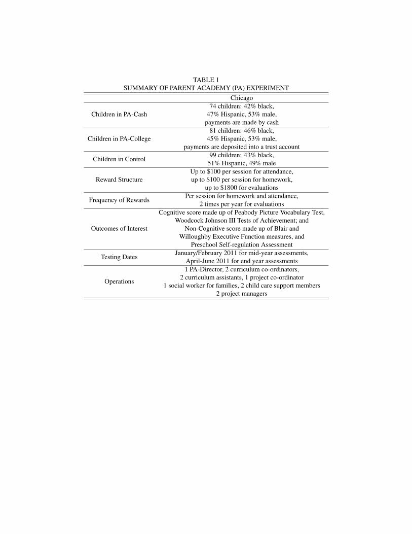
TABLE 1SUMMARY OF PARENT ACADEMY (PA) EXPERIMENT

Chicago

Children in PA-Cash74 children: 42% black,

47% Hispanic, 53% male,payments are made by cash

Children in PA-College81 children: 46% black,

45% Hispanic, 53% male,payments are deposited into a trust account

Children in Control 99 children: 43% black,51% Hispanic, 49% male

Reward StructureUp to $100 per session for attendance,up to $100 per session for homework,

up to $1800 for evaluations

Frequency of Rewards Per session for homework and attendance,2 times per year for evaluations

Outcomes of Interest

Cognitive score made up of Peabody Picture Vocabulary Test,Woodcock Johnson III Tests of Achievement; and

Non-Cognitive score made up of Blair andWilloughby Executive Function measures, and

Preschool Self-regulation Assessment

Testing Dates January/February 2011 for mid-year assessments,April-June 2011 for end year assessments

Operations

1 PA-Director, 2 curriculum co-ordinators,2 curriculum assistants, 1 project co-ordinator

1 social worker for families, 2 child care support members2 project managers

TABLE 2Sample Accounting for All Outcomes

Whole Sample Control Cash CollegeRandomization Sample 260 99 74 87Experimental Sample 254 99 74 81Standardized End Year Cognitive Score 184 73 57 54Standardized End Year Non-Cognitive Score 192 79 57 56

Analysis Sample 193 79 58 56Percentage Sample with at least one outcome 0.760 0.798 0.784 0.691

Notes: This table describes how we obtain different samples from the randomization sample. The first row tabulates all children who wererandomized to get treatment in 2011-2012. The second row tabulates all children who were present in the randomization sample excluding siblingswho belonged to the same treatment. This is done to make sure that all children that are included in the regressions have equal probability ofgetting randomized into treatment. We call this the experimental sample. The third row displays the number of children from the experimentalsample who have non-missing end-year cognitive scores. The fourth row displays the number of children from the experimental sample who havenon-missing end-year non-cognitive scores. The first row from the bottom panel calculates the number of children that have either a non-missingend-year congitive score or a non-missing end-year non-cognitive score. The final row calculates the percentage of children from the experimentalsample that have at least one non missing end-year test score.

TABLE 3SUMMARY STATISTICS

Experimental Sample Analysis SampleControl PA-Cash PA-College p-value Control PA-Cash PA-College p-value

Variable (1) (2) (3) (4) (5) (6) (7) (8)

Age 4.018 4.079 4.012 0.712 3.969 4.039 4.035 0.710Male 0.485 0.527 0.525 0.817 0.557 0.586 0.518 0.766Female 0.515 0.473 0.475 0.817 0.443 0.414 0.482 0.766White 0.061 0.108 0.087 0.524 0.063 0.121 0.071 0.523Black 0.434 0.419 0.463 0.859 0.468 0.379 0.464 0.530Hispanic 0.505 0.473 0.450 0.762 0.468 0.500 0.464 0.914Mother’s age 30.481 32.092 31.833 0.327 30.859 31.529 30.667 0.806Pre treatment cognitive score 43.424 42.504 46.484 0.539 45.219 41.005 47.548 0.310Pre treatment non-cognitive score 0.569 0.567 0.517 0.145 0.572 0.547 0.546 0.606Missing race 0.000 0.000 0.012 0.318 0.000 0.000 0.000 .Missing mother’s age 0.202 0.122 0.185 0.314 0.190 0.121 0.196 0.426Missing pre treatment cognitive score 0.232 0.243 0.235 0.986 0.215 0.276 0.250 0.713Missing pre treatment non-cognitive score 0.030 0.054 0.049 0.690 0.038 0.069 0.036 0.692

p-value from joint F-test 0.723 0.835Observations 99 74 81 79 58 56

Notes: This table descrobes summary statistics and balance tests for baseline observable data. Column (1) reports means for all children in controlgroup for 2011-2012. Columns (2) and (3) report means for children in cash treatment and college treatment groups for 2011-2012. Column(4) reports the p-value from a test of equal means obtained by regressing each variable on treatment dummies and correcting standard errors forheteroskedasticity. Columns (5)-(8) reflect columns (1)-(4) but only for children who have at least one non missing outcome variable i.e. have eithera non missing end of year cognitive score or a non missing end of year no cognitive score.

TABLE 4MEAN EFFECT SIZES (ITT AND LATE ESTIMATES), END YEAR

ITT LATE(1) (2)

A. Standardized Cognitive ScoreCash: 0.073 0.079

(0.104) (0.109)College: 0.166 0.184

(0.113) (0.120)p value: 0.396 0.361

Pooled Treatment: 0.119 0.131(0.094) (0.099)

Observations 184 184

B. Standardized Non-Cognitive ScoreCash: 0.210** 0.225**

(0.101) (0.104)College: 0.197** 0.217**

(0.098) (0.104)p value: 0.903 0.947

Pooled Treatment: 0.203** 0.221**(0.083) (0.088)

Observations 192 192

Notes: This table presents the estimates of the effects of being offered or attending parent academy on standardized end of year cognitive andnon-cognitive scores in 2011-2012. Column (1) reports Intent-To-Treat (ITT) estimates while column (2) reports 2SLS estimates and use treatmentassignment to instrument for the fraction of Parent Academy sessions attended in the year. The dependent variable is the cognitive score or non-cognitive score standardized by year to have a mean of zero and a standard deviation of one. All specifications adjust for the child-level and parent-level demographic variables summarized in Table 3, pre-treatment cognitive and non-cognitive scores and missing indicators for them. Standarderrors (reported in parentheses) are corrected for heteroskedasticity. *, **, and *** denote significance at the 90%, 95% and 99% confidence levels,respectively.

TABLE 5Mean Effect Sizes on Cognitive and Executive Function Indices

Within Demographic SubgroupsStandardized

p-value Observations Standardizedp-value ObservationsCognitive Score Non-Cognitive Score

(1) (2) (3) (4) (5) (6)Whole Sample 0.131 0.185 184 0.221** 0.012 192

(0.099) (0.088)Race

Black -0.234* 0.082 80 -0.059 0.648 85(0.134) (0.129)

Hispanic 0.367*** 0.006 89 0.428*** 0.000 92(0.133) (0.122)

White 0.932*** 0.008 15 0.821*** 0.000 15(0.353) (0.181)

GenderMale 0.107 0.394 102 0.087 0.509 107

(0.126) (0.131)Female 0.056 0.642 82 0.272** 0.010 85

(0.121) (0.106)Parent Income

Parent Income: Above Median -0.013 0.918 95 0.070 0.509 99(0.130) (0.106)

Parent Income: Below Median 0.163 0.360 47 0.502** 0.012 51(0.178) (0.201)

Mother’s AgeMother’s age: Above Median -0.017 0.877 73 0.033 0.805 79

(0.107) (0.132)Mother’s age: Below Median 0.071 0.687 79 0.257** 0.050 80

(0.176) (0.131)Children in the Household

Children in the Household: Above Median 0.310** 0.044 68 0.172 0.263 70(0.154) (0.153)

Children in the Household: Below Median -0.125 0.349 92 0.243** 0.042 97(0.133) (0.120)

TABLE 5Mean Effect Sizes on Cognitive and Executive Function Indices

Within Demographic SubgroupsStandardized

p-value Observations Standardizedp-value ObservationsCognitive Score Non-Cognitive Score

(1) (2) (3) (4) (5) (6)Whole Sample 0.131 0.185 184 0.221** 0.012 192

(0.099) (0.088)

Pre Treatment ScoreCognitive ≥ Median -0.055 0.713 71 0.225** 0.019 74

(0.149) (0.096)Cognitive < Median 0.263* 0.071 68 0.255* 0.096 71

(0.145) (0.153)

Non-Cognitive ≥ Median 0.272** 0.045 90 0.366*** 0.000 93(0.136) (0.100)

Non-Cognitive < Median 0.039 0.809 85 -0.019 0.896 90(0.160) (0.146)

Cog ≥ Median, Non-Cog ≥ Median 0.187 0.343 47 0.335*** 0.001 48(0.197) (0.103)

Cog ≥ Median, Non-Cog < Median -0.419** 0.027 23 0.062 0.574 25(0.190) (0.111)

Cog < Median, Non-Cog ≥ Median 0.343** 0.043 36 0.469*** 0.001 38(0.169) (0.146)

Cog < Median, Non-Cog < Median 0.128 0.621 31 -0.138 0.633 32(0.259) (0.288)

Notes: This table presents the estimates of the effects of attending parent academy on standardized end of year cognitive and non-cognitive scoresin 2011-2012. Columns (1)-(3) report 2SLS estimates on standardized cogntive score while column (4)-(6) report 2SLS estimates on standardizednon cognitive score. The dependent variable is the cognitive score or non-cognitive score standardized by year to have a mean of zero and a standarddeviation of one. All specifications adjust for the child-level and parent-level demographic variables summarized in Table 3, pre-treatment cognitiveand non-cognitive scores and missing indicators for them. Standard errors (reported in parentheses) are corrected for heteroskedasticity. *, **, and*** denote significance at the 90%, 95% and 99% confidence levels, respectively.

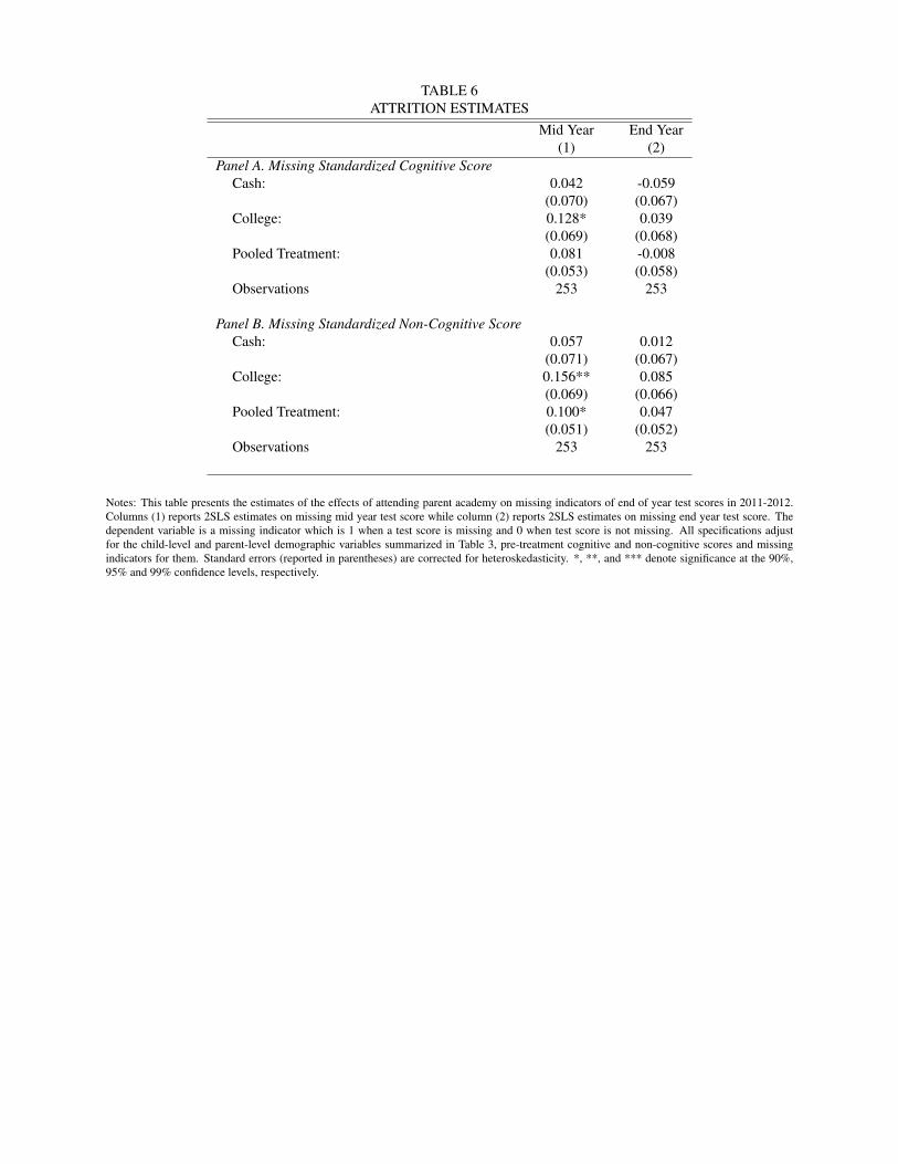
TABLE 6ATTRITION ESTIMATES

Mid Year End Year(1) (2)

Panel A. Missing Standardized Cognitive ScoreCash: 0.042 -0.059

(0.070) (0.067)College: 0.128* 0.039

(0.069) (0.068)Pooled Treatment: 0.081 -0.008

(0.053) (0.058)Observations 253 253

Panel B. Missing Standardized Non-Cognitive ScoreCash: 0.057 0.012

(0.071) (0.067)College: 0.156** 0.085

(0.069) (0.066)Pooled Treatment: 0.100* 0.047

(0.051) (0.052)Observations 253 253

Notes: This table presents the estimates of the effects of attending parent academy on missing indicators of end of year test scores in 2011-2012.Columns (1) reports 2SLS estimates on missing mid year test score while column (2) reports 2SLS estimates on missing end year test score. Thedependent variable is a missing indicator which is 1 when a test score is missing and 0 when test score is not missing. All specifications adjustfor the child-level and parent-level demographic variables summarized in Table 3, pre-treatment cognitive and non-cognitive scores and missingindicators for them. Standard errors (reported in parentheses) are corrected for heteroskedasticity. *, **, and *** denote significance at the 90%,95% and 99% confidence levels, respectively.

TABLE 7LEE BOUND ESTIMATES

LATE LEE p-value(1) (2) (1)=(2)

Mid Year Cogntitive ScorePooled Treatment 0.102 0.003

(0.091) (0.088) 0.006Observations 196 189

End Year Cognitive ScorePooled Treatment 0.131 0.131

(0.099) (0.099) .Observations 184 184

Mid Year Non-Cognitive ScorePooled Treatment 0.119 -0.004

(0.096) (0.085) 0.010Observations 198 191

End Year Non-Cognitive ScorePooled Treatment 0.221** 0.167**

(0.088) (0.081) 0.124Observations 192 190

Notes: This table presents bounded estimates to provide a conservative bound on the true treatment effects under the assumption that these aredifferential attrition rates in the treatment and control groups. Columns (1) reports 2SLS estimates on test scores while column (2) reports the Leebound estimates on test scores. Column (3) reports the p-value for the difference in the estimates reported in columns (1) and (2). The dependentvariable is the cognitive score or non-cognitive score standardized by year to have a mean of zero and a standard deviation of one. All specificationsadjust for the child-level and parent-level demographic variables summarized in Table 3, pre-treatment cognitive and non-cognitive scores andmissing indicators for them. Standard errors (reported in parentheses) are corrected for heteroskedasticity. *, **, and *** denote significance at the90%, 95% and 99% confidence levels, respectively.

TABLE 8AVERAGES BY RACE

Whole Black Hispanic p-value(2) = (3)

(1) (2) (3) (4)

Panel A. Parent InvolvementNo. of sessions attended 8.174 8.333 7.744 0.779No. of sessions parent arrived late to 0.004 0.006 0.003 0.055No.of homework assignments turned in 10.242 10.134 10.197 0.913Average grade in homework 2.902 2.876 2.913 0.070Total amount of money earned from homework assignments 954.444 932.687 952.394 0.837

Panel B. DemographicsParent income 3.938 3.839 3.711 0.501Mother’s age 31.405 32.594 29.747 0.226No. of children in the household 2.459 2.455 2.485 0.572Pre treatment cognitive score 44.136 49.428 39.416 0.014Pre treatment non-cognitive score 0.552 0.552 0.564 0.247

Notes: This table presents means for parent involvement and parent demographic variables. All variables are explain in detail in online AppendixB. Columns (1) reports means for the whole sample in 2011-2012, column (2) reports means for Black children and column (3) reports means forHispanic children. Column (4) reports the p-value for a test of equal means reported in columns (2) and (3).

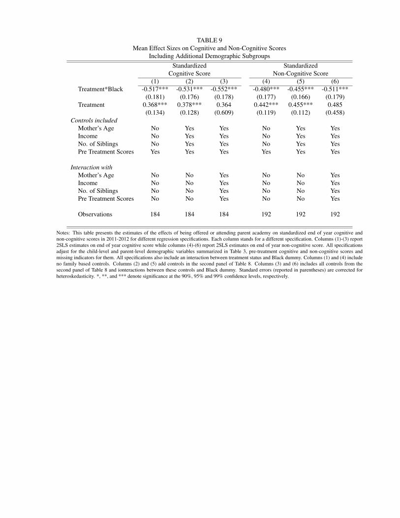
TABLE 9Mean Effect Sizes on Cognitive and Non-Cognitive Scores

Including Additional Demographic SubgroupsStandardized Standardized

Cognitive Score Non-Cognitive Score(1) (2) (3) (4) (5) (6)

Treatment*Black -0.517*** -0.531*** -0.552*** -0.480*** -0.455*** -0.511***(0.181) (0.176) (0.178) (0.177) (0.166) (0.179)

Treatment 0.368*** 0.378*** 0.364 0.442*** 0.455*** 0.485(0.134) (0.128) (0.609) (0.119) (0.112) (0.458)

Controls includedMother’s Age No Yes Yes No Yes YesIncome No Yes Yes No Yes YesNo. of Siblings No Yes Yes No Yes YesPre Treatment Scores Yes Yes Yes Yes Yes Yes

Interaction withMother’s Age No No Yes No No YesIncome No No Yes No No YesNo. of Siblings No No Yes No No YesPre Treatment Scores No No Yes No No Yes

Observations 184 184 184 192 192 192

Notes: This table presents the estimates of the effects of being offered or attending parent academy on standardized end of year cognitive andnon-cognitive scores in 2011-2012 for different regression specifications. Each column stands for a different specification. Columns (1)-(3) report2SLS estimates on end of year cognitive score while columns (4)-(6) report 2SLS estimates on end of year non-cognitive score. All specificationsadjust for the child-level and parent-level demographic variables summarized in Table 3, pre-treatment cognitive and non-cognitive scores andmissing indicators for them. All specifications also include an interaction between treatment status and Black dummy. Columns (1) and (4) includeno family based controls. Columns (2) and (5) add controls in the second panel of Table 8. Columns (3) and (6) includes all controls from thesecond panel of Table 8 and ionteractions between these controls and Black dummy. Standard errors (reported in parentheses) are corrected forheteroskedasticity. *, **, and *** denote significance at the 90%, 95% and 99% confidence levels, respectively.

APPENDIX TABLE 1PARENT ACADEMY CURRICULUM FOR EACH SESSION

Session Executive Function

1 Review of Key EF Concepts2 Mental Functioning3 The Importance of Language4 Socially Shared Cognition5 Learning and Development6 Introduction to Private Speech and Self-talk7 Understanding and Fostering Temperament and Self-Regulation8 Establishing and Fostering Independence9 Fostering Self-Esteem and Moral Development10 Developing Reasoning and Problem Solving skills11 Attention, Approval and Affection12 Parenting Styles and Its Influences on Your Child13 Guidance and Discipline Strategies for Your Child14 Introduction to Parental Intervention15 Resilence and Stress16 Learning How and When to Remove Support17 School Readiness - Rules and Routines in Kindergarten18 Final Review and Wrap-up

Session Literacy and Math

1 Review of Key Lit and Math Concepts2 The Building Blocks of Building Vocabulary3 Having Conversation with Children4 Oral Language and Written Language5 Understanding and Guiding Your Child as They Transition to K6 Reading Readiness-Review of Sound to Symbol Correspondence7 Reading Readiness-Emgerent Reading and Storytelling8 Reading Readiness-Listening to Stories for Fun and to Obtain Information9 School Readiness-Writing, Literacy and Math10 Writing- Salient Sounds Represented by Symbols11 Writing-Expressing Emotions and Communicating through Emergent Writing12 Learning How and When to Remove Support13 Groups of Objects and Numeracy14 Geometry and Constructng 3-D Shapes15 Problems Solving, Computation, Operations16 Graphing/Estimation17 School Readiness - Rules and Routines in Kindergarten18 Final Review and Wrap-up

APPENDIX TABLE 2TIMELINE FOR DATA COLLECTION

Month Collection Method Data Collected

January 2011 - Family Registrations (i) RaceRandomization 2011 (ii) Gender

(iii) Age

May-June 2011 Pre-Assessment Tests (i) Baseline Cognitive Score(ii) Baseline Non-Cognitive Score

May-June 2011 Parent Demographic Survey (i) Parent demographics

January-February 2012 Mid Year Assessment (i) Mid Year Cognitive ScoreTest (ii) Mid Year Non-Cogntitive Score

January-February 2012 Mid Year (i) Survey variablesParent Investment Survey

April-June 2012 End Year Assessment (i) End Year Cognitive ScoreTest (ii) End Year Non-Cogntitive Score

May-June 2012 End Year (i) Survey variablesParent Investment Survey

APPENDIX TABLE 3FIRST STAGE RESULTS

Mid Year End Year(1) (2)

Standardized Cognitive ScoreCash: 0.887*** 0.913***

(0.029) (0.025)F-stat 238.723 605.580

College: 0.871*** 0.902***(0.028) (0.020)

F-stat 163.975 234.304

Pooled Treatment: 0.884*** 0.909***(0.021) (0.017)

F-stat 319.496 464.039

Observations 196 184

Standardized Non-Cognitive ScoreCash: 0.889*** 0.929***

(0.029) (0.018)F-stat 233.763 870.232

College: 0.870*** 0.906***(0.030) (0.019)

F-stat 156.532 242.321

Pooled Treatment: 0.885*** 0.919***(0.021) (0.013)

F-stat 311.800 594.298

Observations 198 192

APPENDIX TABLE 4MEAN EFFECT SIZES (ITT AND LATE ESTIMATES), MID YEAR

ITT LATE(1) (2)

A. Standardized Cognitive ScoreCash: 0.088 0.097

(0.091) (0.097)College: 0.092 0.106

(0.111) (0.122)p value: 0.970 0.942

Pooled Treatment: 0.090 0.102(0.084) (0.091)

Observations 196 196

B. Standardized Non-Cognitive ScoreCash: 0.183* 0.205**

(0.096) (0.103)College: 0.028 0.033

(0.115) (0.128)p value: 0.199 0.195

Pooled Treatment: 0.106 0.119(0.088) (0.096)

Observations 198 198

APPENDIX TABLE 5MEAN EFFECT SIZES FOR TEST OBJECTIVES (LATE ESTIMATES)

WholeSample Black Hispanic p-val

(1) (2) (3) (4)Panel A. WJ Letter Word Idenitification

Cash: 0.152 0.101 0.164(0.145) (0.206) (0.229) 0.837

College: 0.014 -0.176 0.119(0.165) (0.202) (0.274) 0.386

p value: 0.386 0.172 0.859

Pooled Treatment: 0.082 -0.059 0.144(0.134) (0.179) (0.218) 0.473

Observations 193 85 92

Panel B. WJ Applied ProblemsCash: 0.125 -0.235 0.412**

(0.158) (0.268) (0.187) 0.048College: 0.279* -0.315 0.833***

(0.167) (0.225) (0.214) 0.000p value: 0.362 0.767 0.058

Pooled Treatment: 0.203 -0.281 0.602***(0.138) (0.205) (0.169) 0.001

Observations 193 85 92

Panel C. WJ SpellingCash: 0.212 -0.138 0.470**

(0.148) (0.215) (0.210) 0.043College: 0.299* -0.157 0.672***

(0.158) (0.199) (0.223) 0.006p value: 0.607 0.929 0.377

Pooled Treatment: 0.256** -0.149 0.561***(0.128) (0.176) (0.183) 0.005

Observations 193 85 92

Panel D. WJ Quantitative ConceptsCash: 0.174 0.023 0.261

(0.158) (0.244) (0.200) 0.451College: 0.168 -0.240 0.592***

(0.165) (0.230) (0.228) 0.010p value: 0.974 0.267 0.148

Pooled Treatment: 0.171 -0.130 0.406**(0.137) (0.206) (0.180) 0.050

Observations 189 82 91

Panel E. Peabody Picture Vocabulary TestCash: -0.226* -0.470** -0.089

(0.137) (0.198) (0.173) 0.147College: 0.044 -0.479** 0.556**

(0.185) (0.202) (0.273) 0.002p value: 0.142 0.964 0.016

Pooled Treatment: -0.090 -0.475*** 0.213(0.136) (0.174) (0.186) 0.007

Observations 189 83 91

APPENDIX TABLE 6MEAN EFFECT SIZES FOR TEST OBJECTIVES (LATE ESTIMATES)

WholeSample Black Hispanic p-val

(1) (2) (3) (4)Panel A. Preschool Self Regulation Assessment

Cash: -0.221 -0.396 0.191(0.177) (0.257) (0.176) 0.059

College: 0.024 -0.265 0.349**(0.170) (0.269) (0.164) 0.052

p value: 0.197 0.657 0.410

Pooled Treatment: -0.097 -0.321 0.263*(0.147) (0.221) (0.142) 0.026

Observations 193 85 92

Panel B. Operation SpanCash: 0.637*** 0.478** 0.619***

(0.140) (0.194) (0.205) 0.617College: 0.484*** 0.273 0.486**

(0.147) (0.184) (0.229) 0.467p value: 0.290 0.317 0.540

Pooled Treatment: 0.560*** 0.360** 0.559***(0.125) (0.161) (0.188) 0.422

Observations 192 85 92

Panel C. Spatial ConflictCash: 0.204 -0.267 0.467**

(0.161) (0.242) (0.237) 0.030College: 0.137 -0.177 0.457*

(0.166) (0.210) (0.275) 0.067p value: 0.698 0.725 0.968

Pooled Treatment: 0.170 -0.215 0.462**(0.139) (0.186) (0.221) 0.019

Observations 193 85 92

APPENDIX TABLE 7The Amount of Selection on Unobservables Relative to Selection on Observables

Required to Attribute Treatment Effect to Selection BiasWhole Sample Blacks Hispanics

Implied Bias Implied Ratio Implied Bias Implied Ratio Implied Bias Implied Ratio(1) (2) (3) (4) (5) (6)

End Year Cognitive Score -0.005 -22.251 -0.034 6.395 0.032 10.149

End Year Non-Cognitive Score -0.059 -3.419 -0.033 1.656 0.003 147.854

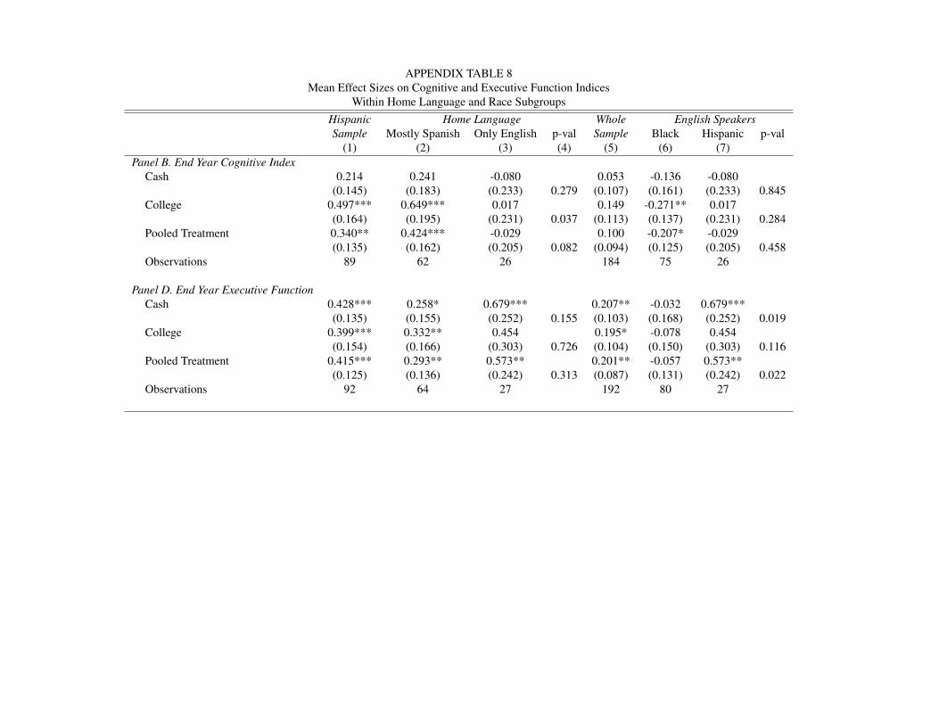
APPENDIX TABLE 8Mean Effect Sizes on Cognitive and Executive Function Indices

Within Home Language and Race SubgroupsHispanic Home Language Whole English SpeakersSample Mostly Spanish Only English p-val Sample Black Hispanic p-val

(1) (2) (3) (4) (5) (6) (7)Panel B. End Year Cognitive Index

Cash 0.214 0.241 -0.080 0.053 -0.136 -0.080(0.145) (0.183) (0.233) 0.279 (0.107) (0.161) (0.233) 0.845

College 0.497*** 0.649*** 0.017 0.149 -0.271** 0.017(0.164) (0.195) (0.231) 0.037 (0.113) (0.137) (0.231) 0.284

Pooled Treatment 0.340** 0.424*** -0.029 0.100 -0.207* -0.029(0.135) (0.162) (0.205) 0.082 (0.094) (0.125) (0.205) 0.458

Observations 89 62 26 184 75 26

Panel D. End Year Executive FunctionCash 0.428*** 0.258* 0.679*** 0.207** -0.032 0.679***

(0.135) (0.155) (0.252) 0.155 (0.103) (0.168) (0.252) 0.019College 0.399*** 0.332** 0.454 0.195* -0.078 0.454

(0.154) (0.166) (0.303) 0.726 (0.104) (0.150) (0.303) 0.116Pooled Treatment 0.415*** 0.293** 0.573** 0.201** -0.057 0.573**

(0.125) (0.136) (0.242) 0.313 (0.087) (0.131) (0.242) 0.022Observations 92 64 27 192 80 27

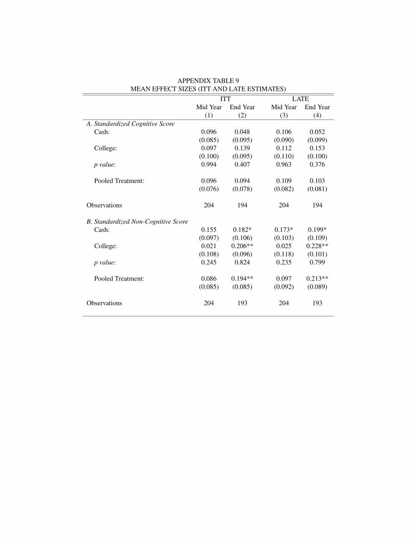
APPENDIX TABLE 9MEAN EFFECT SIZES (ITT AND LATE ESTIMATES)

ITT LATEMid Year End Year Mid Year End Year

(1) (2) (3) (4)A. Standardized Cognitive Score

Cash: 0.096 0.048 0.106 0.052(0.085) (0.095) (0.090) (0.099)

College: 0.097 0.139 0.112 0.153(0.100) (0.095) (0.110) (0.100)

p value: 0.994 0.407 0.963 0.376

Pooled Treatment: 0.096 0.094 0.109 0.103(0.076) (0.078) (0.082) (0.081)

Observations 204 194 204 194

B. Standardized Non-Cognitive ScoreCash: 0.155 0.182* 0.173* 0.199*

(0.097) (0.106) (0.103) (0.109)College: 0.021 0.206** 0.025 0.228**

(0.108) (0.096) (0.118) (0.101)p value: 0.245 0.824 0.235 0.799

Pooled Treatment: 0.086 0.194** 0.097 0.213**(0.085) (0.085) (0.092) (0.089)

Observations 204 193 204 193

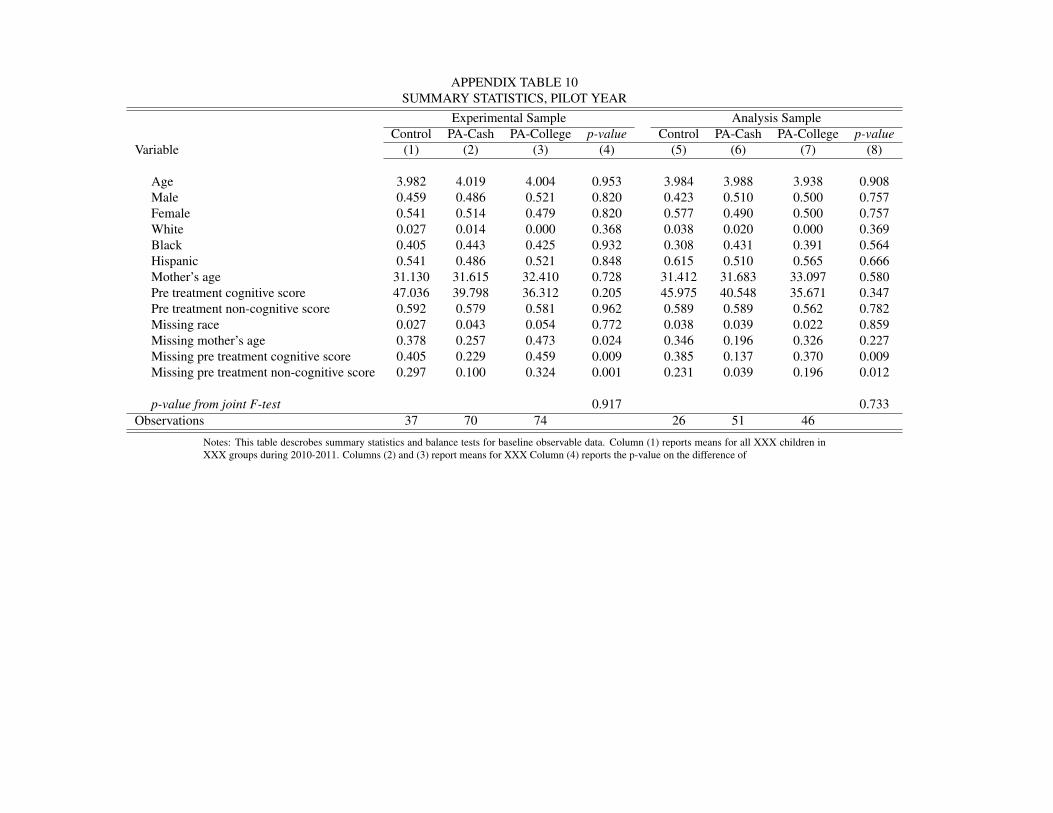
APPENDIX TABLE 10SUMMARY STATISTICS, PILOT YEAR

Experimental Sample Analysis SampleControl PA-Cash PA-College p-value Control PA-Cash PA-College p-value

Variable (1) (2) (3) (4) (5) (6) (7) (8)

Age 3.982 4.019 4.004 0.953 3.984 3.988 3.938 0.908Male 0.459 0.486 0.521 0.820 0.423 0.510 0.500 0.757Female 0.541 0.514 0.479 0.820 0.577 0.490 0.500 0.757White 0.027 0.014 0.000 0.368 0.038 0.020 0.000 0.369Black 0.405 0.443 0.425 0.932 0.308 0.431 0.391 0.564Hispanic 0.541 0.486 0.521 0.848 0.615 0.510 0.565 0.666Mother’s age 31.130 31.615 32.410 0.728 31.412 31.683 33.097 0.580Pre treatment cognitive score 47.036 39.798 36.312 0.205 45.975 40.548 35.671 0.347Pre treatment non-cognitive score 0.592 0.579 0.581 0.962 0.589 0.589 0.562 0.782Missing race 0.027 0.043 0.054 0.772 0.038 0.039 0.022 0.859Missing mother’s age 0.378 0.257 0.473 0.024 0.346 0.196 0.326 0.227Missing pre treatment cognitive score 0.405 0.229 0.459 0.009 0.385 0.137 0.370 0.009Missing pre treatment non-cognitive score 0.297 0.100 0.324 0.001 0.231 0.039 0.196 0.012

p-value from joint F-test 0.917 0.733Observations 37 70 74 26 51 46

Notes: This table descrobes summary statistics and balance tests for baseline observable data. Column (1) reports means for all XXX children inXXX groups during 2010-2011. Columns (2) and (3) report means for XXX Column (4) reports the p-value on the difference of

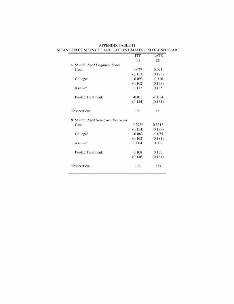
APPENDIX TABLE 11MEAN EFFECT SIZES (ITT AND LATE ESTIMATES), PILOT-END YEAR

ITT LATE(1) (2)

A. Standardized Cognitive ScoreCash: 0.077 0.091

(0.153) (0.173)College: -0.093 -0.110

(0.162) (0.178)p value: 0.173 0.135

Pooled Treatment: -0.011 -0.014(0.144) (0.161)

Observations 121 121

B. Standardized Non-Cognitive ScoreCash: 0.292* 0.351*

(0.154) (0.179)College: -0.063 -0.075

(0.162) (0.181)p value: 0.004 0.002

Pooled Treatment: 0.108 0.130(0.146) (0.164)

Observations 123 123

APPENDIX TABLE 12Mean Effect Sizes on Cognitive and Executive Function Indices

Within Demographic Subgroups, Pilot YearStandardized

p-value Observations Standardizedp-value ObservationsCognitive Score Non-Cognitive Score

(1) (2) (3) (4) (5) (6)Whole Sample -0.014 0.933 121 0.130 0.428 123

(0.161) (0.164)Race

Black -0.338* 0.093 48 -0.525** 0.035 48(0.201) (0.249)

Hispanic 0.194 0.366 67 0.503** 0.032 68(0.215) (0.234)

GenderMale -0.172 0.506 58 0.296 0.376 60

(0.258) (0.334)Female 0.009 0.964 63 -0.029 0.875 63

(0.210) (0.182)Parent Income

Parent Income: Above Median -0.002 0.990 56 0.116 0.600 57(0.176) (0.222)

Parent Income: Below Median -0.297 0.135 27 -0.486* 0.085 27(0.199) (0.282)

Mother’s AgeMother’s age: Above Median -0.025 0.917 47 -0.012 0.962 48

(0.239) (0.256)Mother’s age: Below Median -0.079 0.635 41 0.280 0.220 41

(0.166) (0.228)Children in the Household

Children in the Household: Above Median -0.167 0.586 49 -0.181 0.586 49(0.306) (0.332)

Children in the Household: Below Median -0.067 0.641 44 0.489** 0.018 45(0.145) (0.206)

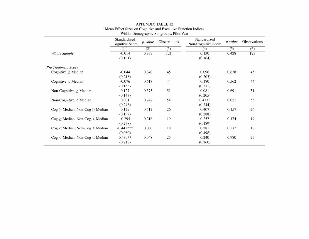
APPENDIX TABLE 12Mean Effect Sizes on Cognitive and Executive Function Indices

Within Demographic Subgroups, Pilot YearStandardized

p-value Observations Standardizedp-value ObservationsCognitive Score Non-Cognitive Score

(1) (2) (3) (4) (5) (6)Whole Sample -0.014 0.933 121 0.130 0.428 123

(0.161) (0.164)

Pre Treatment ScoreCognitive ≥ Median -0.044 0.840 45 0.096 0.638 45

(0.218) (0.203)Cognitive < Median -0.076 0.617 44 0.180 0.562 44

(0.153) (0.311)Non-Cognitive ≥ Median 0.127 0.375 51 0.081 0.691 51

(0.143) (0.205)Non-Cognitive < Median 0.081 0.742 54 0.477* 0.051 55

(0.246) (0.244)Cog ≥ Median, Non-Cog ≥ Median 0.129 0.512 26 0.407 0.157 26

(0.197) (0.288)Cog ≥ Median, Non-Cog < Median -0.294 0.216 19 0.257 0.174 19

(0.238) (0.189)Cog < Median, Non-Cog ≥ Median -0.441*** 0.000 18 0.281 0.572 18

(0.080) (0.498)Cog < Median, Non-Cog < Median 0.430** 0.048 25 0.240 0.780 25

(0.218) (0.860)

APPENDIX TABLE 13MEAN EFFECT SIZES FOR TEST OBJECTIVES (LATE ESTIMATES), PILOT YEAR

WholeSample Black Hispanic p-val

(1) (2) (3) (4)Panel A. WJ Letter Word Idenitification

Cash: 0.045 -0.320 0.424(0.225) (0.262) (0.328) 0.076

College: -0.082 -0.259 0.142(0.229) (0.350) (0.273) 0.366

p value: 0.484 0.857 0.212

Pooled Treatment: -0.019 -0.292 0.253(0.208) (0.255) (0.276) 0.147

Observations 124 49 68

Panel B. WJ Applied ProblemsCash: 0.254 -0.133 0.576*

(0.246) (0.416) (0.309) 0.171College: -0.237 -0.651 -0.013

(0.270) (0.545) (0.272) 0.295p value: 0.007 0.112 0.015

Pooled Treatment: 0.000 -0.390 0.219(0.239) (0.445) (0.265) 0.239

Observations 123 48 68

Panel C. WJ SpellingCash: 0.387* -0.181 0.725**

(0.229) (0.359) (0.293) 0.050College: 0.208 -0.375 0.374

(0.221) (0.342) (0.247) 0.076p value: 0.332 0.405 0.116

Pooled Treatment: 0.294 -0.277 0.512**(0.203) (0.321) (0.240) 0.049

Observations 123 48 68

Panel D. WJ Quantitative ConceptsCash: 0.093 -0.417 0.212

(0.247) (0.294) (0.339) 0.161College: 0.006 -0.085 -0.029

(0.252) (0.343) (0.296) 0.901p value: 0.660 0.391 0.243

Pooled Treatment: 0.048 -0.252 0.063(0.229) (0.265) (0.296) 0.428

Observations 121 48 67

Panel E. Peabody Picture Vocabulary TestCash: 0.072 0.015 0.101

(0.228) (0.343) (0.309) 0.853College: -0.111 -0.792** 0.103

(0.222) (0.387) (0.251) 0.052p value: 0.335 0.016 0.992

Pooled Treatment: -0.021 -0.352 0.102(0.203) (0.311) (0.250) 0.255

Observations 124 49 68

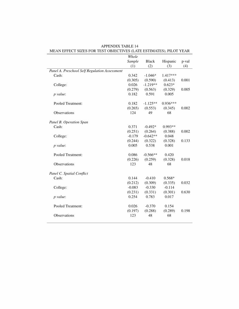
APPENDIX TABLE 14MEAN EFFECT SIZES FOR TEST OBJECTIVES (LATE ESTIMATES), PILOT YEAR

WholeSample Black Hispanic p-val

(1) (2) (3) (4)Panel A. Preschool Self Regulation Assessment

Cash: 0.342 -1.046* 1.417***(0.305) (0.590) (0.413) 0.001

College: 0.026 -1.219** 0.623*(0.279) (0.563) (0.329) 0.005

p value: 0.182 0.591 0.005

Pooled Treatment: 0.182 -1.125** 0.936***(0.265) (0.553) (0.345) 0.002

Observations 124 49 68

Panel B. Operation SpanCash: 0.371 -0.492* 0.993**

(0.251) (0.264) (0.388) 0.002College: -0.179 -0.642** 0.048

(0.244) (0.322) (0.328) 0.133p value: 0.005 0.538 0.001

Pooled Treatment: 0.086 -0.566** 0.420(0.226) (0.259) (0.328) 0.018

Observations 123 48 68

Panel C. Spatial ConflictCash: 0.144 -0.410 0.568*

(0.212) (0.309) (0.335) 0.032College: -0.083 -0.330 -0.114

(0.231) (0.331) (0.301) 0.630p value: 0.254 0.783 0.017

Pooled Treatment: 0.026 -0.370 0.154(0.197) (0.288) (0.289) 0.198

Observations 123 48 68

APPENDIX TABLE 15ATTRITION ESTIMATES BASED ON MID YEAR SCORES

Treatment ControlEnd-Year Score End Year Score

Not Missing Missing Not Missing Missing(1) (2) (3) (4)

Panel A. Standardized Mid Year Cognitive ScoreObservations 99 15 66 16Mean Score 0.099 -0.209 0.086 -0.374Mean Gain: 0.025 -0.126 0.033 -0.223Fractions of Sessions Attended 0.928 0.522 . .

Panel B. Standardized Mid Year Non-Cognitive ScoreObservations 101 13 74 10Mean Score 0.075 -0.093 -0.066 0.192Mean Gain: 0.076 -0.293 -0.155 0.275Fractions of Sessions Attended 0.930 0.470 . .