PASSCoDe: Parallel ASynchronous Stochasticdual Co-ordinate Descent

Cho-Jui HsiehUniversity of Texas, Austin

cjhsieh@cs.utexas.edu

Hsiang-Fu YuUniversity of Texas, Austin

rofuyu@cs.utexas.edu

Inderjit S. DhillonUniversity of Texas, Austin

inderjit@cs.utexas.edu

AbstractStochastic Dual Coordinate Descent (DCD) has become one of the most efficient ways to solve the

family of `2-regularized empirical risk minimization problems, including linear SVM, logistic regres-sion, and many others. The vanilla implementation of DCD is quite slow; however, by maintainingprimal variables while updating dual variables, the time complexity of DCD can be significantly re-duced. Such a strategy forms the core algorithm in the widely-used LIBLINEAR package. In this paper,we parallelize the DCD algorithms in LIBLINEAR. In recent research, several synchronized parallelDCD algorithms have been proposed, however, they fail to achieve good speedup in the shared memorymulti-core setting. In this paper, we propose a family of parallel asynchronous stochastic dual coordinatedescent algorithms (PASSCoDe). Each thread repeatedly selects a random dual variable and conductscoordinate updates using the primal variables that are stored in the shared memory. We analyze the con-vergence properties of DCD when different locking/atomic mechanisms are applied. For implementationwith atomic operations, we show linear convergence under mild conditions. For implementation withoutany atomic operations or locking, we present the first backward error analysis for PASSCoDe under themulti-core environment, showing that the converged solution is the exact solution for a primal problemwith perturbed regularizer. Experimental results show that our methods are much faster than previousparallel coordinate descent solvers.

1 Introduction

Given a set of instance-label pairs (xi, yi), i = 1, · · · , n, xi ∈ Rd, yi ∈ R, we focus on the followingempirical risk minimization problem with `2-regularization:

minw∈Rd

P (w) :=1

2‖w‖2 +

n∑i=1

`i(wTxi), (1)

where xi = yixi, `i(·) is the loss function and ‖·‖ is the 2-norm. A large class of machine learning problemscan be formulated as the above optimization problem. Examples include Support Vector Machines (SVMs),logistic regression, ridge regression, and many others. Problem (1) is usually called the primal problem, andcan usually be solved by Stochastic Gradient Descent (SGD) (Zhang, 2004; Shalev-Shwartz et al., 2007),second order methods (Lin et al., 2007), or primal coordinate descent algorithms (Chang et al., 2008; Huanget al., 2009).

Instead of solving the primal problem, another class of algorithms solves the following dual problem of(1):

minα∈Rn

D(α) :=1

2

∥∥∥∥∥n∑i=1

αixi

∥∥∥∥∥2

+n∑i=1

`∗i (−αi), (2)

1

where `∗i (·) is the conjugate of the loss function `i(·), defined by `∗i (u) = maxz(zu− `i(z)). If we define

w(α) =

n∑i=1

αixi, (3)

then it is known that w(α∗) = w∗ and P (w∗) = −D(α∗) where w∗,α∗ are the optimal primal/dualsolutions respectively. Examples include hinge-loss SVM, square hinge SVM and `2-regularized logisticregression.

Stochastic Dual Coordinate Descent (DCD) has become the most widely-used algorithm for solving (2),and it is faster than primal solvers (including SGD) in many large-scale problems. The success of DCDis mainly due to the trick of maintaining the primal variables w based on the primal-dual relationship (3).By maintaining w in memory, Hsieh et al. (2008); Keerthi et al. (2008) showed that the time complexity ofeach coordinate update can be reduced from O(nnz) to O(nnz/n), where nnz is number of nonzeros in thetraining dataset. Several DCD algorithms for different machine learning problems are currently implementedin LIBLINEAR (Fan et al., 2008) and they are now widely used in both academia and industry. The successof DCD has also catalyzed a large body of theoretical studies (Nesterov, 2012; Shalev-Shwartz & Zhang,2013).

In this paper, we parallelize the DCD algorithm in a shared memory multicore system. There are twothreads of work on parallel coordinate descent. The first thread focuses on synchronized algorithms, in-cluding synchronized CD (Richtarik & Takac, 2012; Bradley et al., 2011) and synchronized DCD algo-rithms (Yang, 2013; Jaggi et al., 2014). However, choosing the block size is a trade-off problem betweencommunication and convergence speed, so synchronous algorithms usually suffer from slower convergence.To overcome this problem, the other thread of work focuses on asynchronous CD algorithms in multi-coreshared memory systems (Liu & Wright, 2014; Liu et al., 2014). However, none of the existing work main-tains both the primal and dual variables. As a result, the recent asynchronous CD algorithms end up beingmuch slower than the state-of-the-art serial DCD algorithms that maintain both w and α, as in the LIB-LINEAR software. This leads to a challenging question: how to maintaining both primal and dual in anasynchronous and efficient way?

In this paper, we propose the first asynchronous dual coordinate descent (PASSCoDe) algorithms withthe address to the issue for the primal variable maintenance in the shared memory multi-core setting.We carefully discuss and analyze three versions of PASSCoDe: PASSCoDe-Lock, PASSCoDe-Atomic, andPASSCoDe-Wild. In PASSCoDe-Lock, convergence is always guaranteed but the overhead for locking makesit even slower than serial DCD. In PASSCoDe-Atomic, the primal-dual relationship (3) is enforced by atomicwrites to the shared memory; while PASSCoDe-Wild proceeds without any locking and atomic operations,as a result of which the relationship (3) between primal and dual variables can be violated due to memoryconflicts. Our contributions can be summarized below:• We propose and analyze a family of asynchronous parallelization of the most efficient DCD algorithm:

PASSCoDe-Lock, PASSCoDe-Atomic, PASSCoDe-Wild.• We show linear convergence of PASSCoDe-Atomic under certain conditions.• We present a backward error analysis for PASSCoDe-Wild and show that the converged solution is the

exact solution of a primal problem with a perturbed regularizer. Therefore the performance is close-to-optimal on most datasets. To best of our knowledge, this is the first attempt to analyze a parallelmachine learning algorithm with memory conflicts using backward error analysis, which is a standardtool in numerical analysis (Wilkinson, 1961).• Experimental results show that our algorithms (PASSCoDe-Atomic and PASSCoDe-Wild) are much

faster than existing methods. For example, on the webspam dataset, PASSCoDe-Atomic took 2 sec-

2

onds and PASSCoDe-Wild took 1.6 seconds to achieve 99% accuracy, while CoCoA took 11.5 secondsusing 10 threads and LIBLINEAR took 10 seconds using 1 thread to achieve the same accuracy.

2 Related Work

Stochastic Coordinate Descent. Coordinate descent is a classical optimization technique that has beenwell studied for a long time (Bertsekas, 1999; Luo & Tseng, 1992). Recently it has enjoyed renewed interestdue to the success of “stochastic” coordinate descent in real applications (Hsieh et al., 2008; Nesterov, 2012).In terms of theoretical analysis, the convergence of (cyclic) coordinate descent has been studied for a longtime (Luo & Tseng, 1992; Bertsekas, 1999), and Saha & Tewari (2013); Wang & Lin (2014) show globallinear convergence under certain conditions (Saha & Tewari, 2013; Wang & Lin, 2014).

Stochastic Dual Coordinate Descent. Many recent papers (Hsieh et al., 2008; Yu et al., 2011; Shalev-Shwartz & Zhang, 2013) have shown that solving the dual problem using coordinate descent algorithms isfaster on large-scale datasets. The success of SDCD strongly relies on exploiting the primal-dual relationship(3) to speed up the gradient computation in the dual space. DCD has become the state-of-the-art solverimplemented in LIBLINEAR (Fan et al., 2008). In terms of convergence of dual objective function, standardtheoretical guarantees for coordinate descent can be directly applied. Taking a different approach, Shalev-Shwartz & Zhang (2013) presented the convergence rate in terms of duality gap.

Parallel Stochastic Coordinate Descent. In order to conduct coordinate updates in parallel, Richtarik& Takac (2012) studied an algorithm where each processor updates a randomly selected block (or coordi-nate) simultaneously, and Bradley et al. (2011) proposed a similar algorithm for `1-regularized problems.Scherrer et al. (2012) studied parallel greedy coordinate descent. However, the above synchronized methodsusually face a trade-off in choosing the block size. If the block size is small, the load balancing problemleads to slow running time. If the block size is large, the convergence speed becomes much slower or thealgorithm can even diverges. These problems can be resolved by developing an asynchronous algorithm.Asynchronous coordinate descent has been studied by (Bertsekas & Tsitsiklis, 1989), but they require theHessian to be diagonal dominant in order to establish convergence. Recently, Liu et al. (2014); Liu &Wright (2014) proved linear convergence of asynchronous stochastic coordinate descent algorithms underthe essential strong convexity condition and a “bounded staleness” condition, where they consider both“consistent read” and “inconsistent read” models. Avron et al. (2014) showed linear rate of convergence forthe asynchronous randomized Gauss-Seidel updates, which is a special case of coordinate descent on linearsystems.

Parallel Stochastic Dual Coordinate Descent. For solving (5), each coordinate updates only requiresthe global primal variables w and one local dual variable αi, thus algorithms only need to synchronize w.Based on this observation, Yang (2013) proposed to update several coordinates or blocks simultaneouslyand update the globalw, and Jaggi et al. (2014) showed that each block can be solved with other approachesunder the same framework. However, both these parallel DCD methods are synchronized algorithms.

To the best of our knowledge, this paper is the first to propose and analyze asynchronous parallel stochas-tic dual coordinate descent methods. By maintaining a primal solutionw while updating dual variables, ouralgorithm is much faster than the previous asynchronous coordinate descent methods of (Liu & Wright,2014; Liu et al., 2014) for solving the dual problem (2). Our algorithms are also faster than synchronizeddual coordinate descent methods (Yang, 2013; Jaggi et al., 2014) since the latest values ofw can be accessedby all the threads. In terms of theoretical contribution, the inconsistent read model in (Liu & Wright, 2014)cannot be directly applied to our algorithm because each update on αi is based on the shared w vector. Wefurther show linear convergence for PASSCoDe-Atomic, and study the properties of the converged solution

3

for the wild version of our algorithm (without any locking and atomic operations) using a backward erroranalysis. Our algorithm has been successfully applied to solve the collaborative ranking problem (Anony-mous, 2015).

3 Algorithms3.1 Stochastic Dual Coordinate Descent

We first describe the Stochastic Dual Coordinate Descent (DCD) algorithm for solving the dual problem (2).At each iteration, DCD randomly picks a dual variable αi and updates it by minimizing the one variablesubproblem (Eq. (4) in Algorithm 1). Without exploiting the structure of the quadratic term, the subproblemsrequire O(nnz) operations, where nnz is the total number of nonzero elements in the training data, whichcan be substantial. However, ifw(α) that satisfies (3) is maintained in memory, the subproblemD(α+δei)can be written as

D(α+ δei) =1

2‖w + δxi‖2 + `∗i (−(αi + δ)),

and the optimal solution can be computed by

δ∗ = arg minδ

1

2(δ +

wTxi‖xi‖2

)2 +1

‖xi‖2`∗i (−(αi + δ)).

Note that all ‖xi‖ can be pre-computed and are constants. For each coordinate update we only need tosolve a simple one-variable subproblem, and the main computation is in computing wTxi, which requiresO(nnz/n) time. For SVM problems, the subproblem has a closed form solution, while for logistic regressionproblems it has to be solved by an iterative solver (see Yu et al. (2011) for details). The DCD algorithm,which is part of the popular LIBLINEAR package, is described in Algorithm 1.

Algorithm 1 Stochastic Dual Coordinate Descent (DCD)Input: Initial α and w =

∑ni=1 αixi

1: while not converged do2: Randomly pick i3: Update αi ← αi + ∆αi, where

∆αi ← arg minδ

1

2‖w + δxi‖2 + `∗i (−(αi + δ)) (4)

4: Update w by w ← w + ∆αixi5: end while

3.2 Asynchronous Stochastic Dual Coordinate DescentTo parallelize DCD in a shared memory multi-core system, we propose a family of Asynchronous StochasticDual Coordinate Descent (PASSCoDe) algorithms. PASSCoDe is very simple but effective. Each threadrepeatedly run the updates (steps 2 to 4) in Algorithm 1 using w, α, and training data stored in a sharedmemory. The threads do not need to coordinate or synchronize their iterations. The details are shown inAlgorithm 2.

4

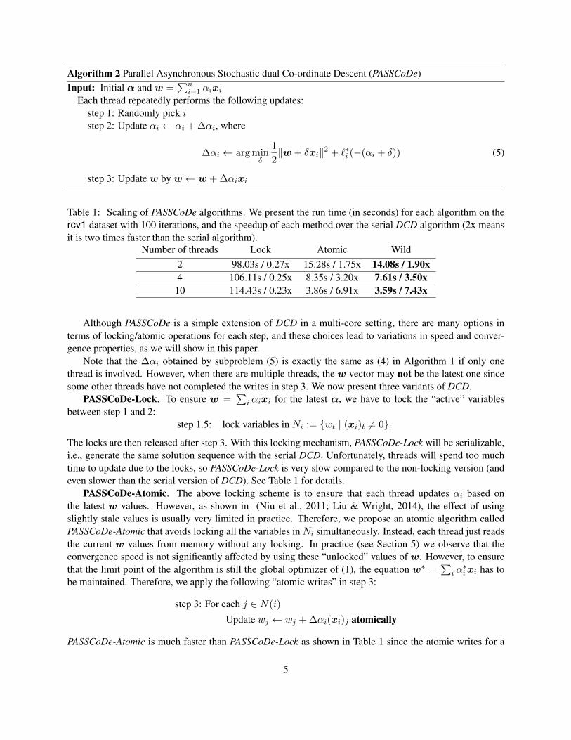
Algorithm 2 Parallel Asynchronous Stochastic dual Co-ordinate Descent (PASSCoDe)Input: Initial α and w =

∑ni=1 αixi

Each thread repeatedly performs the following updates:step 1: Randomly pick istep 2: Update αi ← αi + ∆αi, where

∆αi ← arg minδ

1

2‖w + δxi‖2 + `∗i (−(αi + δ)) (5)

step 3: Update w by w ← w + ∆αixi

Table 1: Scaling of PASSCoDe algorithms. We present the run time (in seconds) for each algorithm on thercv1 dataset with 100 iterations, and the speedup of each method over the serial DCD algorithm (2x meansit is two times faster than the serial algorithm).

Number of threads Lock Atomic Wild2 98.03s / 0.27x 15.28s / 1.75x 14.08s / 1.90x4 106.11s / 0.25x 8.35s / 3.20x 7.61s / 3.50x

10 114.43s / 0.23x 3.86s / 6.91x 3.59s / 7.43x

Although PASSCoDe is a simple extension of DCD in a multi-core setting, there are many options interms of locking/atomic operations for each step, and these choices lead to variations in speed and conver-gence properties, as we will show in this paper.

Note that the ∆αi obtained by subproblem (5) is exactly the same as (4) in Algorithm 1 if only onethread is involved. However, when there are multiple threads, the w vector may not be the latest one sincesome other threads have not completed the writes in step 3. We now present three variants of DCD.

PASSCoDe-Lock. To ensure w =∑

i αixi for the latest α, we have to lock the “active” variablesbetween step 1 and 2:

step 1.5: lock variables in Ni := {wt | (xi)t 6= 0}.

The locks are then released after step 3. With this locking mechanism, PASSCoDe-Lock will be serializable,i.e., generate the same solution sequence with the serial DCD. Unfortunately, threads will spend too muchtime to update due to the locks, so PASSCoDe-Lock is very slow compared to the non-locking version (andeven slower than the serial version of DCD). See Table 1 for details.

PASSCoDe-Atomic. The above locking scheme is to ensure that each thread updates αi based onthe latest w values. However, as shown in (Niu et al., 2011; Liu & Wright, 2014), the effect of usingslightly stale values is usually very limited in practice. Therefore, we propose an atomic algorithm calledPASSCoDe-Atomic that avoids locking all the variables in Ni simultaneously. Instead, each thread just readsthe current w values from memory without any locking. In practice (see Section 5) we observe that theconvergence speed is not significantly affected by using these “unlocked” values of w. However, to ensurethat the limit point of the algorithm is still the global optimizer of (1), the equation w∗ =

∑i α∗ixi has to

be maintained. Therefore, we apply the following “atomic writes” in step 3:

step 3: For each j ∈ N(i)

Update wj ← wj + ∆αi(xi)j atomically

PASSCoDe-Atomic is much faster than PASSCoDe-Lock as shown in Table 1 since the atomic writes for a

5

Table 2: The performance of PASSCoDe-Wild using w or w for prediction. Results show that w yieldsmuch better prediction accuracy, which justifies our theoretical analysis in Section 4.2.

Prediction Accuracy (%) by# threads w w LIBLINEAR

news204 97.1 96.1

97.18 97.2 93.3

covtype4 67.8 38.0

66.38 67.6 38.0

rcv14 97.7 97.5

97.78 97.7 97.4

webspam4 99.1 93.1

99.18 99.1 88.4

kddb4 88.8 79.7

88.88 88.8 87.7

single variable is much faster than locking all the variables. However, the convergence of PASSCoDe-Atomiccannot be guaranteed by tools previously used. To bridge this gap between practice and theory, we provelinear convergence of PASSCoDe-Atomic under certain conditions in Section 4.

PASSCoDe-Wild. Finally, we consider Algorithm 2 without any locks and atomic operations. Theresulting algorithm, PASSCoDe-Wild, is faster than PASSCoDe-Atomic and PASSCoDe-Lock and can achievealmost linear speedup using a single processing unit. However, due to the memory conflicts in step 3, someof the ”updates” to w will be over-written by other threads. As a result, the w and α outputted by thealgorithm usually do not satisfy Eq (3):

w 6= w :=∑i

αixi, (6)

where w, α are the primal and dual variables outputted by the algorithm, and w defined in (6) is computedfrom α. It is easy to see that α is not the optimal solution of (2). Hence, in the prediction phase it is notclear whether one should use w or w. In Section 4 we show that w is actually the optimal solution of aperturbed primal problem (1) using a backward error analysis, where the loss function is the same and theregularization term is slightly perturbed. As a result, the prediction should be done using w, and this alsoyields much better performance in practice, as shown in Table 2.

We summarize the behavior of the three algorithms in Figure 1. Using locks, the algorithm PASSCoDe-Lock is serializable but very slow (even slower than the serial DCD). In the other extreme, the wild versionwithout any lock and atomic operation has very good speed up, but the behavior can be totally differentfrom the serial DCD. Luckily, in Section 4 we provide the convergence guarantee for PASSCoDe-Atomic,and apply a backward error analysis to show that PASSCoDe-Wild will converge to the solution with thesame loss function with a slightly perturbed regularizer.

3.3 Implementation Details

Deadlock Avoidance. Without a proper implementation, a deadlock can arise in PASSCoDe-Lock becausea thread needs to acquire all the locks associated with Ni. A simple way to avoid deadlock is by associatingan ordering for all the locks such that each thread follows the same ordering to acquire the locks.

6

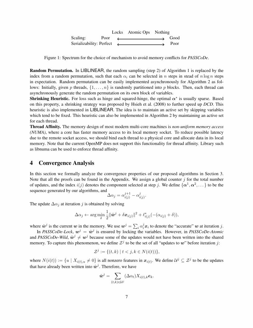
Locks Atomic Ops NothingScaling: Poor GoodSerializability: Perfect Poor

Figure 1: Spectrum for the choice of mechanism to avoid memory conflicts for PASSCoDe.

Random Permutation. In LIBLINEAR, the random sampling (step 2) of Algorithm 1 is replaced by theindex from a random permutation, such that each αi can be selected in n steps in stead of n log n stepsin expectation. Random permutation can be easily implemented asynchronously for Algorithm 2 as fol-lows: Initially, given p threads, {1, . . . , n} is randomly partitioned into p blocks. Then, each thread canasynchronously generate the random permutation on its own block of variables.Shrinking Heuristic. For loss such as hinge and squared-hinge, the optimal α∗ is usually sparse. Basedon this property, a shrinking strategy was proposed by Hsieh et al. (2008) to further speed up DCD. Thisheuristic is also implemented in LIBLINEAR. The idea is to maintain an active set by skipping variableswhich tend to be fixed. This heuristic can also be implemented in Algorithm 2 by maintaining an active setfor each thread.Thread Affinity. The memory design of most modern multi-core machines is non-uniform memory access(NUMA), where a core has faster memory access to its local memory socket. To reduce possible latencydue to the remote socket access, we should bind each thread to a physical core and allocate data in its localmemory. Note that the current OpenMP does not support this functionality for thread affinity. Library suchas libnuma can be used to enforce thread affinity.

4 Convergence Analysis

In this section we formally analyze the convergence properties of our proposed algorithms in Section 3.Note that all the proofs can be found in the Appendix. We assign a global counter j for the total numberof updates, and the index i(j) denotes the component selected at step j. We define {α1,α2, . . . } to be thesequence generated by our algorithms, and

∆αj = αj+1i(j) − α

ji(j).

The update ∆αj at iteration j is obtained by solving

∆αj ← arg minδ

1

2‖wj + δxi(j)‖2 + `∗i(j)(−(αi(j) + δ)),

where wj is the currentw in the memory. We usewj =∑

i αjixi to denote the “accurate”w at iteration j.

In PASSCoDe-Lock, wj = wj is ensured by locking the variables. However, in PASSCoDe-Atomicand PASSCoDe-Wild, wj 6= wj because some of the updates would not have been written into the sharedmemory. To capture this phenomenon, we define Zj to be the set of all “updates to w” before iteration j:

Zj := {(t, k) | t < j, k ∈ N(i(t))},

where N(i(t)) := {u | Xi(t),u 6= 0} is all nonzero features in xi(t). We define U j ⊆ Zj to be the updatesthat have already been written into wj . Therefore, we have

wj =∑

(t,k)∈Uj

(∆αt)Xi(t),kek.

7

4.1 Linear Convergence of PASSCoDe-Atomic

In PASSCoDe-Atomic, we assume all the updates before the (j − τ)-th iteration has been written into wj ,therefore,

Assumption 1. The set U j satisfies Zj−τ ⊆ U j ⊆ Zj .

Now we define some constants used in our theoretical analysis. Note that X ∈ Rn×d is the data matrix,and we use X ∈ Rn×d to denote the normalized data matrix where each row is xTi = xTi /‖xi‖2. We thendefine

Mi = maxS⊆[d]

‖∑t∈S

X:,tXi,t‖, M = maxiMi,

where [d] := {1, . . . , d} is the set of all the feature indices, and X:,t is the t-th column of X . We also defineRmin = mini ‖xi‖2, Rmax = maxi ‖xi‖2, and Lmax to be the Lipschitz constant such that ‖∇D(α1) −∇D(α2)‖ ≤ Lmax‖α1 − α2‖ for all α1,α2 within the level set {α | D(α) ≤ D(α0)}. We assume thatRmax = 1 and there is no zero training sample, so Rmin > 0.

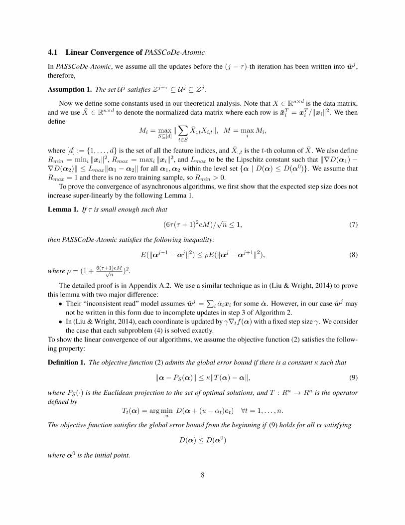
To prove the convergence of asynchronous algorithms, we first show that the expected step size does notincrease super-linearly by the following Lemma 1.

Lemma 1. If τ is small enough such that

(6τ(τ + 1)2eM)/√n ≤ 1, (7)

then PASSCoDe-Atomic satisfies the following inequality:

E(‖αj−1 −αj‖2) ≤ ρE(‖αj −αj+1‖2), (8)

where ρ = (1 + 6(τ+1)eM√n

)2.

The detailed proof is in Appendix A.2. We use a similar technique as in (Liu & Wright, 2014) to provethis lemma with two major difference:• Their “inconsistent read” model assumes wj =

∑i αixi for some α. However, in our case wj may

not be written in this form due to incomplete updates in step 3 of Algorithm 2.• In (Liu & Wright, 2014), each coordinate is updated by γ∇tf(α) with a fixed step size γ. We consider

the case that each subproblem (4) is solved exactly.To show the linear convergence of our algorithms, we assume the objective function (2) satisfies the follow-ing property:

Definition 1. The objective function (2) admits the global error bound if there is a constant κ such that

‖α− PS(α)‖ ≤ κ‖T (α)−α‖, (9)

where PS(·) is the Euclidean projection to the set of optimal solutions, and T : Rn → Rn is the operatordefined by

Tt(α) = arg minu

D(α+ (u− αt)et) ∀t = 1, . . . , n.

The objective function satisfies the global error bound from the beginning if (9) holds for all α satisfying

D(α) ≤ D(α0)

where α0 is the initial point.

8

This definition is a generalized version of Definition 6 in (Wang & Lin, 2014). We list several importantmachine learning problems that admit global error bounds:

• Support Vector Machines (SVM) with hinge loss (Boser et al., 1992):

`i(zi) = C max(1− zi, 0)

`∗i (−αi) =

{−αi if 0 ≤ αi ≤ C,∞ otherwise.

(10)

• Support Vector Machines (SVM) with square hinge loss:

`i(zi) = C max(1− zi, 0)2

`∗i (−αi) =

{−αi + α2

i /4C if αi ≥ 0,

∞ otherwise.(11)

• Logistic Regression:

`i(zi) = C log(1 + e−zi

)`∗i (−αi) =

{αi log(αi) + (C − αi) log(C − αi) if 0 ≤ αi ≤ C,∞ otherwise,

(12)

where we use the convention that 0 log 0 = 0.

Note that C > 0 is the penalty parameter that controls the weights between loss and regularization.

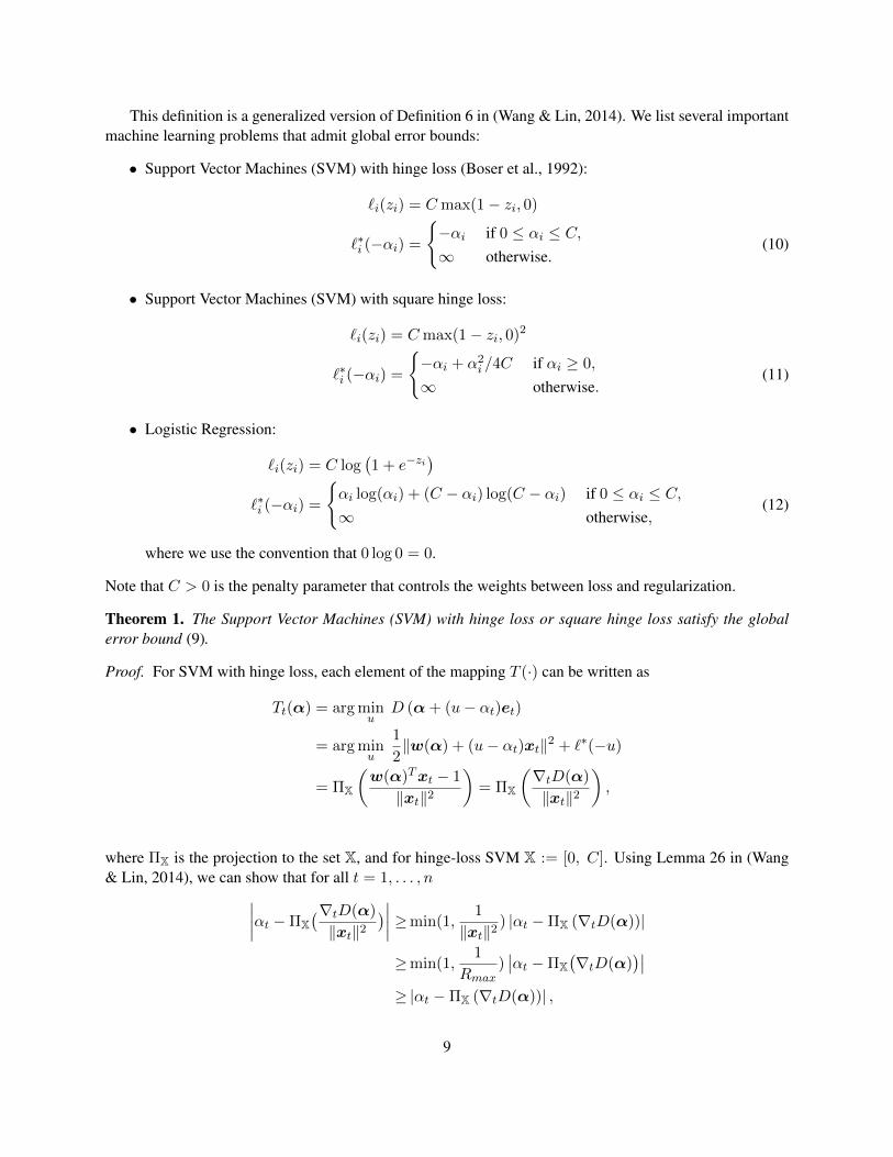
Theorem 1. The Support Vector Machines (SVM) with hinge loss or square hinge loss satisfy the globalerror bound (9).

Proof. For SVM with hinge loss, each element of the mapping T (·) can be written as

Tt(α) = arg minu

D (α+ (u− αt)et)

= arg minu

1

2‖w(α) + (u− αt)xt‖2 + `∗(−u)

= ΠX

(w(α)Txt − 1

‖xt‖2

)= ΠX

(∇tD(α)

‖xt‖2

),

where ΠX is the projection to the set X, and for hinge-loss SVM X := [0, C]. Using Lemma 26 in (Wang& Lin, 2014), we can show that for all t = 1, . . . , n∣∣∣∣αt −ΠX

(∇tD(α)

‖xt‖2)∣∣∣∣ ≥min(1,

1

‖xt‖2) |αt −ΠX (∇tD(α))|

≥min(1,1

Rmax)∣∣αt −ΠX

(∇tD(α)

)∣∣≥ |αt −ΠX (∇tD(α))| ,

9

where the last inequality is due to the assumption that Rmax = 1. Therefore,

‖α− T (α)‖2 ≥1√n‖α− T (α)‖1

≥ 1√n

n∑t=1

|αt −ΠX(∇tD(α)

)|

=1√n‖∇+D(α)‖1

≥ 1√n‖∇+D(α)‖2

≥ 1

κ0√n‖α− PS(α)‖2,

where ∇+D(α) is the projected gradient defined in Definition 5 of (Wang & Lin, 2014) and κ0 is the κdefined in Theorem 18 of (Wang & Lin, 2014). Thus, with κ = κ0

√n, we obtain that the dual function of

the hinge-loss SVM satisfies the global error bound defined in Definition 1. Similarly, we can show that theSVM with squared-hinge loss satisfies the global error bound.

Next we explicitly state the linear convergence guarantee for PASSCoDe-Atomic.

Theorem 2. Assume the objective function (2) admits a global error bound from the beginning and theLipschitz constant Lmax is finite in the level set. If (7) holds and

1 ≥ 2LmaxRmin

(1 +

eτM√n

)(τ2M2e2

n

)then PASSCoDe-Atomic has a global linear convergence rate in expectation, that is,

E[D(αj+1)]−D(α∗) ≤ η(E[D(αj)]−D(α∗)

), (13)

where α∗ is the optimal solution and

η = 1− κ

Lmax

(1− 2Lmax

Rmin

(1 +

eτM√n

)(τ2M2e2

n

))(14)

4.2 Backward Error Analysis for PASSCoDe-Wild

In PASSCoDe-Wild, assume the sequence {αj} converges to α and {wj} converges to w. Now we showthat the dual solution α and the corresponding primal variables w =

∑ni=1 αixi are actually the dual and

primal solutions of a perturbed problem:

Theorem 3. α is the optimal solution of a perturbed dual problem

α = arg minα

D(α)−n∑i=1

αiεTxi, (15)

and w =∑

i αixi is the solution of the corresponding primal problem:

w = arg minw

1

2wTw +

n∑i=1

`i((w − ε)Txi), (16)

where ε ∈ Rd is given by ε = w − w.

10

Proof. By definition, α is the limit point of PASSCoDe-Wild. Therefore, {∆αi} → 0 for all i. Combiningwith the fact that {wj} → w, we have

−wTxi ∈ ∂αi`∗i (−αi), ∀i.

Since w = w − ε, we have

−(w − ε)Txi ∈ ∂αi`∗i (−αi), ∀i

−wTxi ∈ ∂αi

(`∗i (−αi)− αiεTxi

), ∀i

0 ∈ ∂αi

(1

2‖

n∑i=1

αixi‖2 + `∗i (−αi)− αiεTxi

), ∀i

which is the optimality condition of (14). Thus, α is the optimal solution of (14).For the second part of the theorem, let’s consider the following equivalent primal problem and its La-

grangian:

minw,ξ

1

2wTw +

n∑i=1

`i(ξi) s.t. ξi = (w − ε)Txi ∀i = 1, . . . , n

L(w, ξ,α) :=1

2wTw +

n∑i=1

{`i(ξi) + αi(ξi −wTxi + εTxi)}

The corresponding convex version of the dual function can be derived as follows.

D(α) = maxw,ξ−L(w, ξ,α)

=

(maxw−1

2wTw +

n∑i=1

αiwTxi

)+

n∑i=1

(maxξi−`i(ξi)− αiξi

)− αiεTxi

=1

2‖

n∑i=1

αixi‖2 +

n∑i=1

`∗i (−αi)− αiεTxi

= D(α)−n∑i=1

αiεTxi

The second last equality comes from• the substitution of w∗ =

∑Ti=1 αixi obtained by setting∇w − L(w, ξ,α) = 0; and

• the definition of the conjugate function `∗i (−αi).The second part of the theorem follows.

Note that ε is the error caused by the memory conflicts. From Theorem 3, w is the optimal solutionof the “biased” primal problem (15), however, in (15) the actual model that fits the loss function should bew = w− ε. Therefore after the training process we should use w to predict, which is thew we maintainedduring the parallel coordinate descent updates. Replacing w by w − ε in (15), we have the followingcorollary :

Corollary 1. w computed by PASSCoDe-Wild is the solution of the following perturbed primal problem:

w = arg minw

1

2(w + ε)T (w + ε) +

n∑i=1

`i(wTxi) (17)

11

Table 3: Data statistics. n is the number of test instances. d is the average nnz per instance.n n d d C

news20 16,000 3,996 1,355,191 455.5 2covtype 500,000 81,012 54 11.9 0.0625rcv1 677,399 20,242 47,236 73.2 1webspam 280,000 70,000 16,609,143 3727.7 1kddb 19,264,097 748,401 29,890,095 29.4 1

The above corollary shows that the computed primal solution w is actually the exact solution of a per-turbed problem (where the perturbation is on the regularizer). This strategy (of showing that the computedsolution to a problem is the exact solution of a perturbed problem) is inspired by the backward error analysistechnique commonly employed in numerical analysis (Wilkinson, 1961)1.

5 Experimental Results

We conduct several experiments and show that the proposed PASSCoDe-Atomic and PASSCoDe-Wild havesuperior performance compared to other state-of-the-art parallel coordinate descent algorithms. We considerfive datasets: news20, covtype, rcv1, webspam, and kddb. Detailed information is shown in Table 3. Tohave a fair comparison, we implement all methods in C++ using OpenMP as the parallel programmingframework. All the experiments are performed on an Intel multi-core dual-socket machine with 256 GBmemory. Each socket is associated with 10 computation cores. We explicitly enforce that all the threads usecores from the same socket to avoid inter-socket communication. Our codes will be publicly available. Wefocus on solving SVM with hinge loss in the experiments, but the algorithms can also be applied to otherobjective functions.

Serial Baselines.• DCD: we implement Algorithm 1. Instead of sampling with replacement, a random permutation is

used to enforce random sampling without replacement.• LIBLINEAR: we use the implementation in http://www.csie.ntu.edu.tw/˜cjlin/liblinear.

This implementation is equivalent to DCD with the shrinking strategy.Compared Parallel Implementation.• PASSCoDe: We implement the proposed three variants of Algorithm 2 using DCD as the building

block: Wild, Atomic, and Lock.• CoCoA: We implement a multi-core version of CoCoA (Jaggi et al., 2014) with βK = 1 and DCD as

its local dual method.• AsySCD: We follow the description in (Liu & Wright, 2014; Liu et al., 2014) to implement AsySCD

with the step length γ = 12 and the shuffling period p = 10 as suggested in (Liu et al., 2014).

5.1 Convergence in terms of iterations.

The primal objective function value is used to determine the convergence. Note that we still use P (w) forPASSCoDe-Wild, although the true primal objective should be (16). As long as wT ε remains small enough,the trends of (16) and P (w) are similar.

1J. H. Wilkinson received the Turing Award in 1970, partly for his work on backward error analysis

12

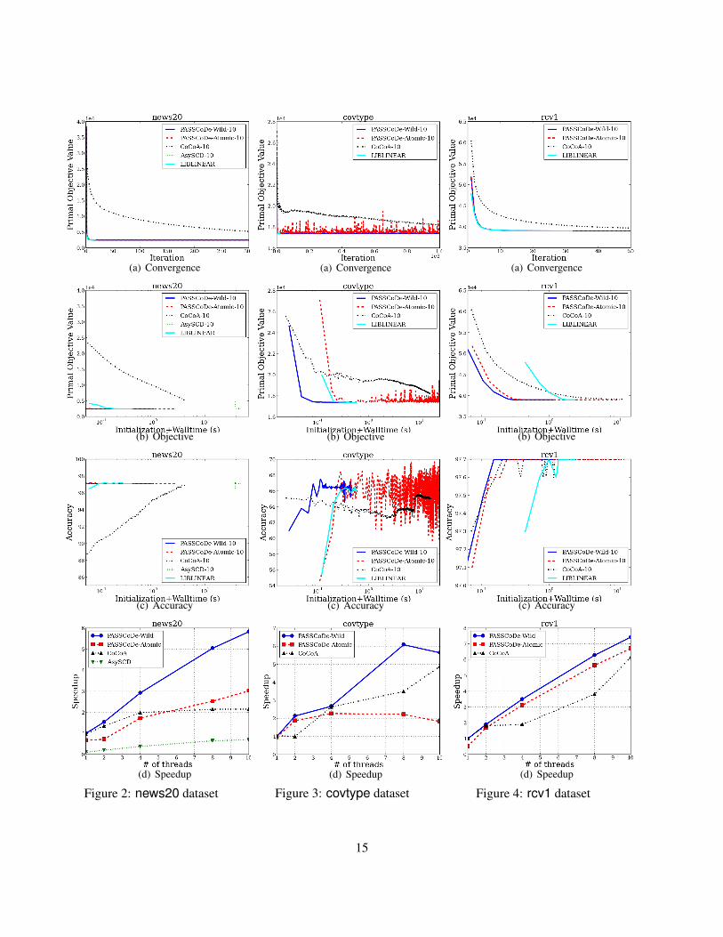
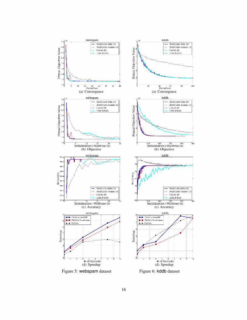
Figures 2(a), 3(a), 4(a), 5(a), 6(a) show the convergence results of PASSCoDe-Wild, PASSCoDe-Atomic,CoCoA, and AsySCD with 10 threads in terms of number of iterations. The horizontal line in grey indicatesthe primal objective function value obtained by LIBLINEAR using the default stopping condition. The resultfor LIBLINEAR is also included for reference. We make the following observations:• Convergence of three PASSCoDe variants are almost identical and very close to the convergence

behavior of serial LIBLINEAR on three large sparse datasets (rcv1, webspam, and kddb).• PASSCoDe-Wild and PASSCoDe-Atomic converge significantly faster than CoCoA.• On covtype, a more dense dataset, all three algorithms (PASSCoDe-Wild, PASSCoDe-Atomic, and

CoCoA) have slower convergence.

5.2 Efficiency

Timing. To have a fair comparison, we include both initialization and computation into the timing results.For DCD, PASSCoDe, and CoCoA, initialization takes one pass of entire data matrix (which is O(nnz(X)))to compute ‖xi‖ for each instance. In the initialization stage, AsySCD requires O(n × nnz(X)) time andO(n2) space to form and store the Hessian matrix Q for (2). Thus, we only have results on news20 forAsySCD as all other datasets are too large for AsySCD to fit Q in even 256 GB memory. Note that we alsoparallelize the initialization part for each algorithm in our implementation to have a fair comparison.

Figures 2(b), 3(b), 4(b), 5(b), 6(b) show the primal objective values in terms of time and Figures 2(c),3(c), 4(c), 5(c), 6(c) shows the accuracy in terms of time. Note that the x-axis for news20, covtype, andrcv1 is in log-scale. A horizontal line in gray in each figure denotes the objective values/accuracy obtainedby LIBLINEAR using the default stopping condition. We have the following observations:• From Figures 2(b) and 2(c), we can see that AsySCD is orders of magnitude slower than other ap-

proaches including parallel methods and serial reference (AsySCD using 10 cores takes 0.4 secondsto run 10 iterations, while all the other parallel approaches takes less than 0.14 seconds, and LIBLIN-EAR takes less than 0.3 seconds). In fact, AsySCD is still slower than other methods even when theinitialization time is excluded. This is expected because AsySCD is a parallel version of a standardcoordinate descent method, which is known to be much slower than DCD for (2). Since AsySCD runsout of memory for all the other larger datasets, we do not show the results in other figures.• In most cases, both PASSCoDe approaches outperform CoCoA. In Figure 6(c), kddb shows better

accuracy performance in the early stage which can be explained by the ensemble nature of CoCoA. Inthe long term, it still converges to the accuracy obtained by LIBLINEAR.• For all datasets, PASSCoDe-Wild is slightly faster than PASSCoDe-Atomic. Given the fact that both

methods show similar convergence in terms of iterations, this phenomenon can be explained by theeffect of atomic operations. We observe that more dense the dataset, larger the difference betweenPASSCoDe-Wild and PASSCoDe-Atomic.

5.3 SpeedupWe are interested in the following evaluation criterion:

speedup :=time taken by the target method with p threadstime taken by the best serial reference method

,

This criterion is different from scaling, where the denominator is replaced by “time taken for the targetmethod with single thread.” Note that a method can have perfect scaling but very poor speedup. Figures2(d), 3(d), 4(d), 5(d), 6(d) shows the speedup results, where 1) DCD is used as the best serial reference; 2)

13

the shrinking heuristic is turned off for all PASSCoDe and DCD to have fair comparison; 3) the initializationtime is excluded from the computation of speedup.• PASSCoDe-Wild has very good speedup performance compared to other approaches. It achieves a

speedup of about about 6 to 8 using 10 threads on all the datasets.• From Figure 2(d), we can see that AsySCD hardly has any “speedup” over the serial reference, al-

though it is shown to have almost linear scaling (Liu et al., 2014; Liu & Wright, 2014).

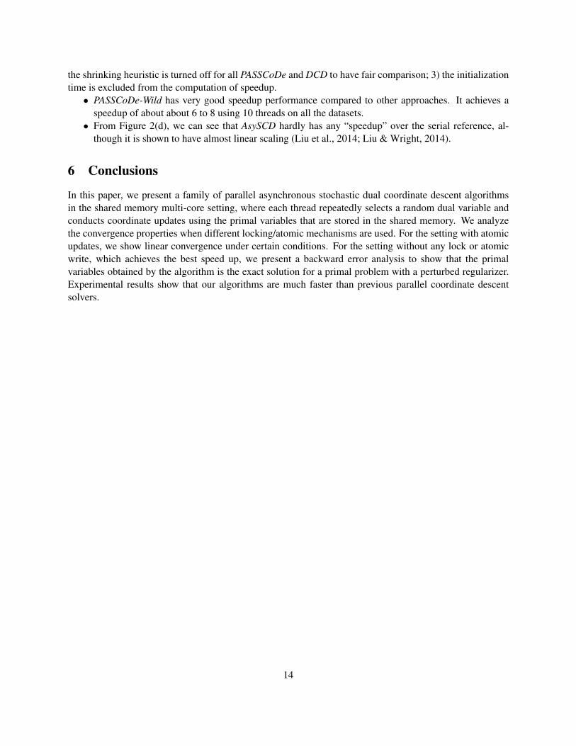
6 Conclusions

In this paper, we present a family of parallel asynchronous stochastic dual coordinate descent algorithmsin the shared memory multi-core setting, where each thread repeatedly selects a random dual variable andconducts coordinate updates using the primal variables that are stored in the shared memory. We analyzethe convergence properties when different locking/atomic mechanisms are used. For the setting with atomicupdates, we show linear convergence under certain conditions. For the setting without any lock or atomicwrite, which achieves the best speed up, we present a backward error analysis to show that the primalvariables obtained by the algorithm is the exact solution for a primal problem with a perturbed regularizer.Experimental results show that our algorithms are much faster than previous parallel coordinate descentsolvers.

14

(a) Convergence

(b) Objective

(c) Accuracy

(d) Speedup

Figure 2: news20 dataset

(a) Convergence

(b) Objective

(c) Accuracy

(d) Speedup

Figure 3: covtype dataset

(a) Convergence

(b) Objective

(c) Accuracy

(d) Speedup

Figure 4: rcv1 dataset

15

(a) Convergence

(b) Objective

(c) Accuracy

(d) Speedup

Figure 5: webspam dataset

(a) Convergence

(b) Objective

(c) Accuracy

(d) Speedup

Figure 6: kddb dataset

16

References

Anonymous. Preference completion: Large-scale collaborative ranking from pairwise comparison. submit-ted to ICML, 2015.

Avron, H., Druinsky, A., and Gupta, A. Revisiting asynchronous linear solvers: Provable convergence ratethrough randomization. In IEEE International Parallel and Distributed Processing Symposium, 2014.

Bertsekas, Dimitri P. Nonlinear Programming. Athena Scientific, Belmont, MA 02178-9998, second edi-tion, 1999.

Bertsekas, Dimitri P. and Tsitsiklis, John N. Parallel and Distributed Computation: Numerical Methods.Prentice Hall, 1989.

Boser, Bernhard E., Guyon, Isabelle, and Vapnik, Vladimir. A training algorithm for optimal margin clas-sifiers. In Proceedings of the Fifth Annual Workshop on Computational Learning Theory, pp. 144–152.ACM Press, 1992.

Bradley, Joseph K., Kyrola, Aapo, Bickson, Danny, and Guestrin, Carlos. Parallel coordinate descent forl1-regularized loss minimization. In ICML, 2011.

Chang, Kai-Wei, Hsieh, Cho-Jui, and Lin, Chih-Jen. Coordinate descent method for large-scale L2-losslinear SVM. Journal of Machine Learning Research, 9:1369–1398, 2008. URL http://www.csie.ntu.edu.tw/˜cjlin/papers/cdl2.pdf.

Fan, Rong-En, Chang, Kai-Wei, Hsieh, Cho-Jui, Wang, Xiang-Rui, and Lin, Chih-Jen. LIBLINEAR: alibrary for large linear classification. JMLR, 9:1871–1874, 2008.

Hsieh, Cho-Jui, Chang, Kai-Wei, Lin, Chih-Jen, Keerthi, S. Sathiya, and Sundararajan, Sellamanickam. Adual coordinate descent method for large-scale linear SVM. In Proceedings of the Twenty Fifth Inter-national Conference on Machine Learning (ICML), 2008. URL http://www.csie.ntu.edu.tw/

˜cjlin/papers/cddual.pdf.

Huang, Fang-Lan, Hsieh, Cho-Jui, Chang, Kai-Wei, and Lin, Chih-Jen. Iterative scaling and coordinatedescent methods for maximum entropy. In Proceedings of the 47th Annual Meeting of the Association ofComputational Linguistics (ACL), 2009. Short paper.

Jaggi, Martin, Smith, Virginia, Takac, Martin, Terhorst, Jonathan, Hofmann, Thomas, and Jordan, Michael I.Communication-efficient distributed dual coordinate ascent. In Advances in Neural Information Process-ing Systems 27. 2014.

Keerthi, S. Sathiya, Sundararajan, Sellamanickam, Chang, Kai-Wei, Hsieh, Cho-Jui, and Lin, Chih-Jen. Asequential dual method for large scale multi-class linear SVMs. In Proceedings of the Forteenth ACMSIGKDD International Conference on Knowledge Discovery and Data Mining, pp. 408–416, 2008. URLhttp://www.csie.ntu.edu.tw/˜cjlin/papers/sdm_kdd.pdf.

Lin, Chih-Jen, Weng, Ruby C., and Keerthi, S. Sathiya. Trust region Newton method for large-scale logisticregression. In Proceedings of the 24th International Conference on Machine Learning (ICML), 2007.Software available at http://www.csie.ntu.edu.tw/˜cjlin/liblinear.

17

Liu, J. and Wright, S. J. Asynchronous stochastic coordinate descent: Parallelism and convergence proper-ties. 2014. URL http://arxiv.org/abs/1403.3862.

Liu, J., Wright, S. J., Re, C., and Bittorf, V. An asynchronous parallel stochastic coordinate descent algo-rithm. In ICML, 2014.

Luo, Zhi-Quan and Tseng, Paul. On the convergence of coordinate descent method for convex differentiableminimization. Journal of Optimization Theory and Applications, 72(1):7–35, 1992.

Nesterov, Yurii E. Efficiency of coordinate descent methods on huge-scale optimization problems. SIAMJournal on Optimization, 22(2):341–362, 2012.

Niu, Feng, Recht, Benjamin, Re, Christopher, and Wright, Stephen J. HOGWILD!: a lock-free approach toparallelizing stochastic gradient descent. In Advances in Neural Information Processing Systems 24, pp.693–701, 2011.

Richtarik, Peter and Takac, Martin. Parallel coordinate descent methods for big data optimization. Mathe-matical Programming, 2012. Under revision.

Saha, Ankan and Tewari, Ambuj. On the nonasymptotic convergence of cyclic coordinate descent methods.SIAM Journal on Optimization, 23(1):576–601, 2013.

Scherrer, C., Tewari, A., Halappanavar, M., and Haglin, D. Feature clustering for accelerating parallelcoordinate descent. In NIPS, 2012.

Shalev-Shwartz, S., Singer, Y., and Srebro, N. Pegasos: primal estimated sub-gradient solver for SVM. InICML, 2007.

Shalev-Shwartz, Shai and Zhang, Tong. Stochastic dual coordinate ascent methods for regularized lossminimization. Journal of Machine Learning Research, 14:567–599, 2013.

Wang, Po-Wei and Lin, Chih-Jen. Iteration complexity of feasible descent methods for convex optimization.Journal of Machine Learning Research, 15:1523–1548, 2014. URL http://www.csie.ntu.edu.tw/˜cjlin/papers/cdlinear.pdf.

Wilkinson, J. H. Error analysis of direct methods of matrix inversion. Journal of the ACM, 1961.

Yang, T. Trading computation for communication: Distributed stochastic dual coordinate ascent. In NIPS,2013.

Yu, Hsiang-Fu, Huang, Fang-Lan, and Lin, Chih-Jen. Dual coordinate descent methods for logistic re-gression and maximum entropy models. Machine Learning, 85(1-2):41–75, October 2011. URLhttp://www.csie.ntu.edu.tw/˜cjlin/papers/maxent_dual.pdf.

Yu, Hsiang-Fu, Hsieh, Cho-Jui, Si, Si, and Dhillon, Inderjit S. Scalable coordinate descent approachesto parallel matrix factorization for recommender systems. In Proceedings of the IEEE InternationalConference on Data Mining, pp. 765–774, 2012.

Zhang, Tong. Solving large scale linear prediction problems using stochastic gradient descent algorithms.In Proceedings of the 21th International Conference on Machine Learning (ICML), 2004.

18

A Linear Convergence for PASSCoDe-Atomic

A.1 Notations and Propositions

A.1.1 Notations

• For all i = 1, . . . , n, we have the following definitions:

hi(u) :=`∗i (−u)

‖xi‖2

proxi(s) := arg minu

1

2(u− s)2 + hi(u)

Ti(w, s) := arg minu

1

2‖w + (u− s)xi‖2 + `∗i (−u)

= arg minu

1

2

[u−

(s− w

Txi‖xi‖2

)]2+ hi(u),

where w ∈ Rd and s ∈ R. For convergence, we define T (w, s) as an n-dimension vector withTi(w, s) = Ti(w, st) as the i-th element. We also denote prox(s) as the proximal operator from Rn

to Rn such that (prox(s))i = proxi(si). We can see the connection of the above operator and theproximal operator: Ti(w, s) = proxi(s− wTxi

‖xi‖2 ).

• Let {αj} and {wj} be the sequence generated/maintained by Algorithm 2 using

αj+1t =

{Tt(w

j , αjt ) if t = i(j),

αjt if t 6= i(j),

where i(j) is the index selected at j-th iteration. For convenience, we define

∆αj = αj+1i(j) − α

ji(j).

• Let {αj} be the sequence defined by

αj+1t = Tt(w

j , αjt ) ∀t = 1, . . . , n.

Note that αj+1i(j) = αj+1

i(t) and αj+1 = prox(αj − Xwj).

• Let wj =∑n

i=1 αjixi be the “true” primal variables corresponding to αj . Thus,

Tt(wj , αi(j)) = T (αj),

where T (·) is the operator defined in Eq. (9).

• Let {βj}, {βj} be the sequences defined by

βj+1t =

{Tt(w

j , αjt ) if t = i(j),

αjt if t 6= i(j),βj+1t = Tt(w

j , αjt ) ∀t = 1, . . . , n.

Note that βj+1i(j) = βj+1

i(j) and βj+1

= T (αj), where T (·) is the operator defined in Eq. (9).

19

• Let gj(u) be the univariate function considered at the j-th iteration:

gj(u) := D(αj + (u− αji(j)) · ei(j)

)=

1

2‖wj + (u− αji(j))xi‖

2 + `∗i (−u) + constant

Thus, βj+1i(j) = Ti(j)(w

j , αji(j)) is the minimizer for gj(u).

A.1.2 Propositions

Proposition 1.

Ei(j)(‖αj+1 −αj‖2

)=

1

n‖αj+1 −αj‖2, (18)

Ei(j)(‖βj+1 −αj‖2

)=

1

n‖βj+1 −αj‖2, (19)

Proof. Based on the assumption that i(j) is uniformly random selected from {1, . . . , n}, the above twoidentities follow from the definition of α and β.

Proposition 2.

‖Xwj − Xwj‖ ≤Mj−1∑t=j−τ

|∆αt|. (20)

Proof.

‖Xwj − Xwj‖ = ‖X(∑

(t,k)∈Zj\Uj

(∆αt)Xi(t),kek)‖ = ‖∑

(t,k)∈Zj\Uj

(∆αt)X:,kXi(t),k‖

≤j−τ∑t=j−1

|∆αt|Mi ≤Mj−1∑t=j−τ

|∆αt|

Proposition 3. For any w1,w2 ∈ Rd and s1, s2 ∈ R,

|Ti(w1, s1)− Ti(w2, s2)| ≤ |s1 − s2 +(w1 −w2)

Txi‖xi‖2

|. (21)

Proof. It can be proved by the connection of Ti(w, s) and proxi(·) and the non-expansiveness of the proxi-mal operator.

Proposition 4. Let M ≥ 1, q = 6(τ+1)eM√n

, ρ = (1 + q)2, and θ =∑τ

t=1 ρt/2. If q(τ + 1) ≤ 1, then

ρ(τ+1)/2 ≤ e, and

ρ−1 ≤ 1− 4 + 4M + 4Mθ√n

. (22)

20

Proof. By the definition of ρ and the condition q(τ + 1) ≤ 1, we have

ρ(τ+1)/2 =

((ρ1/2

)1/q)q(τ+1)

=(

(1 + q)1/q)q(τ+1)

≤ eq(τ+1) ≤ e.

By the definitions of q, we know that

q = ρ1/2 − 1 =6(τ + 1)eM√

n⇒ 3

2=

√n(ρ1/2 − 1)

4(τ + 1)eM.

We can derive

3

2=

√n(ρ1/2 − 1)

4(τ + 1)eM

≤√n(ρ1/2 − 1)

4(τ + 1)ρ(τ+1)/2M∵ ρ(τ+1)/2 ≤ e

≤√n(ρ1/2 − 1)

4(1 + θ)ρ1/2M∵ 1 + θ =

τ∑t=0

ρt/2 ≤ (τ + 1)ρτ/2

=

√n(1− ρ−1/2)4(1 + θ)M

≤√n(1− ρ−1)

4(1 + θ)M∵ ρ−1/2 ≤ 1

Combining the condition that M ≥ 1 and 1 + θ ≥ 1, we have√n(1− ρ−1)− 4

4(1 + θ)M≥√n(1− ρ−1)

4(1 + θ)M− 1

2≥ 1,

which leads to

4(1 + θ)M ≤√n−√nρ−1 − 4

ρ−1 ≤ 1− 4 + 4M + 4Mθ√n

.

Proposition 5. For all j > 0, we have

D(αj) ≥ D(βj+1) +‖xi(j)‖2

2‖αj − βj+1‖2 (23)

D(αj+1) ≤ D(βj+1) +Lmax

2‖αj+1 − βj+1‖2 (24)

Proof. First, two properties of gj(u) are stated as follows.

• the strong convexity of gj(u): as all the conjugate functions are convex, so it is clear that gj(u) is‖xi(j)‖2-strongly convex.

• the Lipschitz continuous gradient of gj(u): it follows from the Lipschitz assumption of∇D(α).

21

With the above two properties of gj(u) and the fact that u∗ := βj+1i(j) is the minimizer of gj(u) (which

implies that∇gj(u∗) = 0), we have the following inequalities:

gj(αji(j)) ≥ gj(βj+1

i(j) ) +‖xi(j)‖2

2‖αji(j) − β

j+1i(j) ‖

2 by strong convexity,

gj(αj+1i(j) ) ≤ gj(βj+1

i(j) ) +Lmax

2‖αj+1

i(j) − βj+1i(j) ‖

2 by Lipschitz continuity.

By the definitions of gj , αj , αj+1, and βj+1, we know that

gj(αji(j))− gj(βj+1

i(j) ) = D(αj)−D(βj+1),

‖αji(j) − βj+1i(j) ‖

2 = ‖αj − βj+1‖2,

gj(αj+1i(j) )− ≤ gj(βj+1

i(j) ) = D(αj+1)−D(βj+1),

‖αj+1i(j) − β

j+1i(j) ‖

2 = ‖αj+1 − βj+1‖2,

which imply (22) and (23).

A.2 Proof of Lemma 1

Similar to Liu & Wright (2014), we prove Eq. (8) by induction. First, we know that for any two vectors aand b, we have

‖a‖2 − ‖b‖2 ≤ 2‖a‖‖b− a‖.

See Liu & Wright (2014) for a proof for the above inequality. Thus, for all j , we have

‖αj−1 − αj‖2 − ‖αj − αj+1‖2 ≤ 2‖αj−1 − αj‖‖αj − αj+1 −αj−1 + αj‖. (25)

The second factor in the r.h.s of (24) is bounded as follows:

‖αj − αj+1 −αj−1 + αj‖≤ ‖αj −αj−1‖+ ‖ prox(αj − Xwj)− prox(αj−1 − Xwj−1)‖≤ ‖αj −αj−1‖+ ‖(αj − Xwj)− (αj−1 − Xwj−1)‖≤ ‖αj −αj−1‖+ ‖αj −αj−1‖+ ‖Xwj − Xwj−1‖= 2‖αj −αj−1‖+ ‖Xwj − Xwj−1‖= 2‖αj −αj−1‖+ ‖Xwj − Xwj + Xwj − Xwj−1 + Xwj−1 − Xwj−1‖≤ 2‖αj −αj−1‖+ ‖Xwj − Xwj−1‖+ ‖Xwj − Xwj‖+ ‖Xwj−1 − Xwj−1‖

≤ (2 +M)‖αj −αj−1‖+

j−1∑t=j−τ

‖∆αt‖M +

j−2∑t=j−τ−1

‖∆αt‖M

= (2 + 2M)‖αj −αj−1‖+ 2M

j−2∑t=j−τ−1

‖∆αt‖ (26)

22

Now we prove (8) by induction.Induction Hypothesis. Using Proposition 1, we prove the following equivalent statement. For all j,

E(‖αj−1 − αj‖2) ≤ ρE(‖αj − αj+1‖2), (27)

Induction Basis. When j = 1,

‖α1 − α2 +α0 − α1‖ ≤ (2 + 2M)‖α1 −α0‖.

Taking the expectation of (24), we have

E[‖α0 − α1‖2]− E[‖α1 − α2‖2] ≤ 2E[‖α0 − α1‖‖α1 − α2 −α0 + α1‖]≤ (4 + 4M)E(‖α0 − α1‖‖α0 −α1‖).

From (17) in Proposition 1, we have E[‖α0 − α1‖2] = 1n‖α

0 − α1‖2. Also, by AM-GM inequality, forany µ1, µ2 > 0 and any c > 0, we have

µ1µ2 ≤1

2(cµ21 + c−1µ22). (28)

Therefore, we have

E[‖α0 − α1‖‖α0 −α1‖]

≤ 1

2E[n1/2‖α0 −α1‖2 + n−1/2‖α1 −α0‖2

]=

1

2E[n−1/2‖α0 − α1‖2 + n−1/2‖α1 −α0‖2

]by (17)

= n−1/2E[‖α0 − α1‖2].

Therefore,

E[‖α0 − α1‖2]− E[‖α1 − α2‖2] ≤ 4 + 4M√n

E[‖α0 − α1‖2],

which implies

E[‖α0 −α1‖2] ≤ 1

1− 4+4M√n

E[‖α1 − α2‖2] ≤ ρE[‖α1 − α2‖2], (29)

where the last inequality is based on Proposition 4 and the fact θM ≥ 1.Induction Step. By the induction hypothesis, we assume

E[‖αt−1 − αt‖2] ≤ ρE[‖αt − αt+1‖2] ∀t ≤ j − 1. (30)

The goal is to showE[‖αj−1 − αj‖2] ≤ ρE[‖αj − αj+1‖2].

First, we show that for all t < j,

E[‖αt −αt+1‖‖αj−1 − αj‖

]≤ ρ(j−1−t)/2√

nE[‖αj−1 − αj‖2

](31)

23

Proof. By (27) with c = n1/2γ, where γ = ρ(t+1−j)/2,

E[‖αt −αt+1‖‖αj−1 − αj‖

]≤ 1

2E[n1/2γ‖αt −αt+1‖2 + n−1/2γ−1‖αj−1 − αj‖2

]=

1

2E[n1/2γE[‖αt −αt+1‖2] + n−1/2γ−1‖αj−1 − αj‖2

]=

1

2E[n−1/2γ‖αt − αt+1‖2 + n−1/2γ−1‖αj−1 − αj‖2

]by Proposition 1

≤ 1

2E[n−1/2γρj−1−t‖αj−1 − αj‖2 + n−1/2γ−1‖αj−1 − αj‖2

]by Eq. (29)

≤ 1

2E[n−1/2γ−1‖αj−1 − αj‖2 + n−1/2γ−1‖αj−1 −αj‖2

]by the definition of γ

≤ ρ(j−1−t)/2√n

E[‖αj−1 − αj‖2

]

Let θ =∑τ

t=1 ρt/2. We have

E[‖αj−1 − αj‖2]− E[‖αj − αj+1‖2]

≤ E[2‖αj−1 − αj‖

((2 + 2M)‖αj −αj−1‖+ 2M

j−1∑t=j−τ−1

‖αt −αt−1‖)]

by (24), (25)

= (4 + 4M)E(‖αj−1 − αj‖‖αj −αj−1‖) + 4M

j−1∑t=j−τ−1

E[‖αj−1 − αj‖‖αt −αt−1‖

]

≤ (4 + 4M)n−1/2E[‖αj −αj−1‖2] + 4Mn−1/2E[‖αj−1 − αj‖2]j−2∑

t=j−1−τρ(j−1−t)/2 by (30)

≤ (4 + 4M)n−1/2E[‖αj −αj−1‖2] + 4Mn−1/2θE[‖αj−1 − αj‖2]

≤ 4 + 4M + 4Mθ√n

E[‖αj−1 − αj‖2],

which implies that

E[‖αj−1 − αj‖2] ≤ 1

1− 4+4M+4Mθ√n

E[‖αj − αj+1‖2] ≤ ρE[‖αj − αj+1‖2],

where the last inequality is based on Proposition 4.

A.3 Proof of Theorem 2

We can bound the expected distance E[‖βj+1 − αj+1‖2

]by the following derivation.

24

E[‖βj+1 − αj+1‖2

]= E

[n∑t=1

(Tt(w

j , αjt )− Tt(wj , αjt )

)2]

≤ E

n∑t=1

((wj − wj

)Txt

‖xt‖2

)2 By Proposition 3

= E[‖X(wj − wj)‖2

]≤M2E

j−1∑t=j−τ

‖αt+1 −αt‖

2 By Proposition 2

≤M2E

τ j−1∑t=j−τ

‖αt+1 −αt‖2 By Cauchy Schwarz Inequality

≤ τM2E

[(τ∑t=1

ρt‖αj −αj+1‖2)]

By Lemma 1

≤ τM2

n

(τ∑t=1

ρt

)E[‖αj+1 −αj‖2

]By Proposition 1

≤ τ2M2

nρτE

[‖αj+1 −αj‖2

]Proposition 4 implies ρ(τ+1)/2 ≤ e, which further implies ρτ ≤ e2 because ρ ≥ 1. Thus,

E[‖βj+1 − αj+1‖2

]≤ τ2M2e2

nE[‖αj+1 −αj‖2

]. (32)

Applying Cauchy-Schwarz Inequality, we obtain

E[‖βj+1 −αj‖2

]= E

[‖βj+1 − αj+1 + αj+1 −αj‖2

]≤ E

[2(‖βj+1 − αj+1‖2 + ‖αj+1 −αj‖2

)]≤ 2

(1 +

e2τ2M2

n

)E[‖αj+1 −αj‖2

]. (33)

Next, we bound the decrease of objective function value by

D(αj)−D(αj+1) =(D(αj)−D(βj+1)

)+(D(βj+1)−D(αj+1)

)≥

(‖xi(j)‖2

2‖αj+1 − βj+1‖2

)−(Lmax

2‖βj+1 −αj+1‖2

)by Proposition 5

≥(Rmin

2‖αj − βj+1‖2

)−(Lmax

2‖βj+1 −αj+1‖2

)

25

So

E[D(αj)]− E[D(αj+1)]

≥ Rmin2n

E[‖βj+1 −αj‖2]− Lmax2n

E[‖βj+1 − αj+1‖2] by Proposition 1

≥ Rmin2n

E[‖βj+1 −αj‖2]− Lmax2n

τ2M2e2

nE[‖αj+1 −αj‖2] by (31)

≥ Rmin2n

E[‖βj+1 −αj‖2]− 2Lmax2n

τ2M2e2

n

(1 +

eτM√n

)E[‖βj+1 −αj‖2] by (32)

≥ Rmin2n

(1− 2Lmax

Rmin

(1 +

eτM√n

)(τ2M2e2

n

))E[‖βj+1 −αj‖2]

Let b =(

1− 2LmaxRmin

(1 + eτM√

n

)(τ2M2e2

n

))and combining the above inequality with Eq (9) we have

E[D(αj)]− E[D(αj+1)] ≥ bκE[‖αj − PS(αj)‖2]

≥ bκ

LmaxE[D(αj)−D∗].

Therefore, we have

E[D(αj+1)]−D∗ = E[D(αj)]−(E[D(αj)]− E[D(αj+1)]

)−D∗

≤ (1− bκ

Lmax)(E[D(αj)]−D∗)

≤ η(E[D(αj)]−D∗

),

where η = 1− bκLmax

.

26