implementation of the uv-vis method to measure … researchers purchased three uv-vis instruments...

Technical Report Documentation . Report No. FHWA/TX-11/5-5540-01-1

2. Government Accession No.

3. Recipient's Catalog No.

4. Title and Subtitle IMPLEMENTATION OF THE UV-VIS METHOD TO MEASURE ORGANIC CONTENT IN CLAY SOILS: TECHNICAL REPORT

5. Report Date October 2010 Published: May 2011

6. Performing Organization Code

7. Author(s) Pat Harris, Omar Harvey, and Stephen Sebesta

8. Performing Organization Report No. Report 5-5540-01-1

9. Performing Organization Name and Address Texas Transportation Institute The Texas A&M University System College Station, Texas 77843-3135

10. Work Unit No. (TRAIS) 11. Contract or Grant No. Project 5-5540-01

12. Sponsoring Agency Name and Address Texas Department of Transportation Research and Technology Implementation Office P. O. Box 5080 Austin, Texas 78763-5080

13. Type of Report and Period Covered Technical Report September 2009–August 2010 14. Sponsoring Agency Code

15. Supplementary Notes Project performed in cooperation with the Texas Department of Transportation and the Federal Highway Administration. Project Title: Implementation of the UV-Vis Method to Measure Content in Clay Soils URL: http://tti.tamu.edu/documents/5-5540-01-1.pdf 16. Abstract The Texas Department of Transportation has been having problems with organic matter in soils that they stabilize for use as subgrade layers in road construction. The organic matter reduces the effectiveness of common soil additives (lime/cement) in stabilization projects. The researchers developed a technique using UV-Vis spectroscopy to measure the harmful organic matter in another project (0-5540). This project consisted of purchasing three UV-Vis instruments, equipping them with software to measure the organic matter and doing two trainings with the Texas Department of Transportation. Following the trainings, four laboratories analyzed 20 natural soil samples and three laboratory standards to determine repeatability and reproducibility between the laboratories. Researchers also continued testing real project soils to see what mitigation techniques researchers could use. Researchers determined that three replicates need to be run to achieve 95 percent confidence that the measured value is the true value. Researchers determined that soils with organic matter below 1.5 percent can be safely treated, and soils with an organic matter to Eades and Grim optimum lime (OM: EG) ratio less than 0.5 have the greatest potential for mitigation with additional lime application. Additionally, calcium chloride added to the soil with the lime improved the formation of pozzolanic reaction products and strengths of some soils. This work illustrates the complex nature of organic interactions with soil stabilizers and the many questions left unresolved. 17. Key Words

Soil Organic Matter, Soil Stabilization, Lime Treatment, Expansive Soils

18. Distribution Statement No restrictions. This document is available to the public through NTIS: National Technical Information Service Alexandria, Virginia 22312http://www.ntis.gov

19. Security Classif.(of this report) Unclassified

20. Security Classif.(of this page) Unclassified

21. No. of Pages 56

22. Price

Form DOT F 1700.7 (8-72) Reproduction of completed page authorize

http://tti.tamu.edu/documents/5-5540-01-1.pdf

http://www.ntis.gov

IMPLEMENTATION OF THE UV-VIS METHOD TO MEASURE

ORGANIC CONTENT IN CLAY SOILS: TECHNICAL REPORT

by

Pat Harris Associate Research Scientist

Texas Transportation Institute

Omar Harvey Graduate Research Assistant


and

Stephen Sebesta Assistant Research Scientist


Report 5-5540-01-1 Project 5-5540-01

Project Title: Implementation of the UV-Vis Method to Measure Content in Clay Soils

Performed in cooperation with the Texas Department of Transportation

and the Federal Highway Administration

October 2010 Published: May 2011

TEXAS TRANSPORTATION INSTITUTE The Texas A&M University System College Station, Texas 77843-3135

v

DISCLAIMER

The contents of this report reflect the views of the authors, who are responsible for the facts and the accuracy of the data presented herein. The contents do not necessarily reflect the official view or policies of the Federal Highway Administration (FHWA) or the Texas Department of Transportation (TxDOT). This report does not constitute a standard, specification, or regulation. The researcher in charge was Pat Harris, P.G. (Texas# 1756).

The United States Government and the state of Texas do not endorse products or

manufacturers. Trade or manufacturers’ names appear herein solely because they are considered essential to the object of this report.

vi

ACKNOWLEDGMENTS

Dr. German Claros, P.E., and Ms. Claudia Izzo from the Texas Department of

Transportation are program coordinator and project director, respectively, of this important project and have been active in providing direction to the research team. Mr. Cliff Coward; Ms. Darlene Goehl, P.E.; Mr. Billy Pigg, P.E.; and Ms. Zyna Polansky from TxDOT, have also been active in assisting the researchers. Both TxDOT and the FHWA provided funds for this project.

vii

TABLE OF CONTENTS

Page List of Figures .............................................................................................................................. viii

List of Tables ................................................................................................................................. ix

Chapter 1. Purchase and Implementation of Three UV-VIS Systems in District Labs ..................1

Introduction ..........................................................................................................................1

Chapter 2. Repeatability Studies with the UV-VIS Equipment ......................................................5

Introduction ..........................................................................................................................5

Data Collection Methods .....................................................................................................5

Discussion of Results ...........................................................................................................7

Conclusions ........................................................................................................................13

Chapter 3. Field and Lab Testing ..................................................................................................15

Introduction ........................................................................................................................15

Methods..............................................................................................................................19

Results ................................................................................................................................20

Discussion ..........................................................................................................................26

Chapter 4. Test Protocol ...............................................................................................................29

Introduction ........................................................................................................................29

Research Questions ............................................................................................................29

Testing Protocol .................................................................................................................30

References ......................................................................................................................................33

Appendix: UV-VIS Method for Detecting Soil Organic Matter (SOM) ......................................35

viii

LIST OF FIGURES

Figure Page

1.1. Pelican Case with UV-Vis Instrumentation. ........................................................................1

1.2. Pelican Case Showing the HP Mini and Software Delivered to TxDOT ............................2

1.3. Measured Sulfate Concentration in Different Soil Samples Using Colorimeter and

UV-Vis Spectrometer: (a) Correlation between Measured Values, (b) Comparison

by Sample Number ..............................................................................................................4

2.1. Repeatability Limits for UV-Vis Organic Matter Tests ......................................................7

2.2. Reproducibility Limits for UV-Vis Organic Matter Tests ...................................................8

2.3. Comparison of UV-Vis with Spoon Results versus Known Values ..................................11

2.4. Comparison of UV-Vis Measurements without Spoon versus Known Values .................12

2.5. Change in Sample Mass with Level when Using Measurement Spoon ............................12

3.1. Web Soil Survey Map along SH 90 Showing OM Contents: Red Stars

Designate Soil Sampling Locations ...................................................................................17

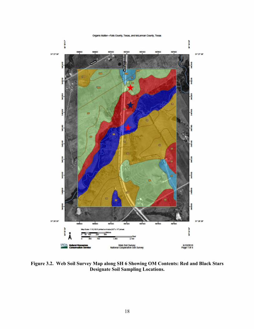
3.2. Web Soil Survey Map along SH 6 Showing OM Contents: Red and

Black Stars Designate Soil Sampling Locations ................................................................18

3.3. Web Soil Survey Map along SH 29 Showing OM Contents: Red and

Black Stars Designate Soil Sampling Locations ................................................................19

3.4. Relative Strength Gains for Soils Stabilized with Lime at 0.5, 1, 1.5, and 2

Times Optimum (EG). Numbers in Parentheses Indicate Percent Organic

Matter in a Given Soil ........................................................................................................22

3.5. Relative Strength Gains for Soils Stabilized with Lime at 0.5, 1, 1.5, and 2 Times

Optimum (EG) + Calcium Chloride (CaCl2.2H2O = 0.25EG).

Organic Matter in Parentheses ...........................................................................................23

3.6. DSC Thermograms of SH 90-3 Soil Treatments Show Evidence of Cementitious

Product Formation .............................................................................................................24

3.7. DSC Thermograms for SH 90-3 Samples Treated with Calcium Chloride Dihydrate .....26

3.8. Relative Strength Gains as a Function of Organic Matter Content: Optimal Lime

Content (OM: EG) for Soils Treated Using Hydrated Lime Only

(0.5EG, EG, 1.5EG, 2EG) .................................................................................................28

ix

LIST OF TABLES

Table Page

1.1. Sulfate Concentration in 20 Soil Samples Measured Using Colorimeter (TX-146-E)

and UV-Vis Equipment (with Updated Software) Provided by Researchers .........................3

2.1. Test Soils and Known Organic Matter Treatment Levels ......................................................5

2.2. Soil Organic Matter Precision Statistics for UV-Vis Test Method Using Spoon ...................6

2.3. Soil Organic Matter Precision Statistics for UV-Vis Test Method without the Spoon ..........6

2.4. Data for Comparing Precision of UV-Vis Methods with and without

Measurement Spoon................................................................................................................8

2.5. Paired T-Test Results for UV-Vis Method with Spoon. .........................................................9

2.6. Paired T-Test Results for UV-Vis Method with Analytical Balance ...................................10

3.1. Properties Reported from the WSS along with Engineering Properties of Soils

Used in This Study ................................................................................................................15

3.2. Physical and Chemical Properties of Soils Selected to Measure Effects of

Organic Matter on Stabilization ............................................................................................16

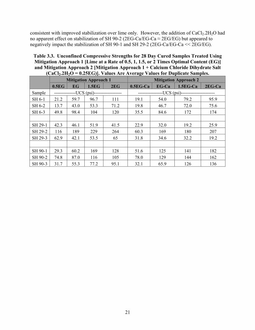
3.3. Unconfined Compressive Strengths for 28 Day Cured Samples Treated Using

Mitigation Approach 1 [Lime at a Rate of 0.5, 1, 1.5, or 2 Times Optimal Content

(EG)] and Mitigation Approach 2 [Mitigation Approach 1 + Calcium Chloride

Dihydrate Salt (CaCl2.2H2O = 0.25EG)]. Values Are Average Values for

Duplicate Samples ................................................................................................................21

3.4. Peak Areas from DSC Attributable to CSH II Formation ....................................................25

1

CHAPTER 1

PURCHASE AND IMPLEMENTATION OF THREE UV-VIS SYSTEMS IN

DISTRICT LABS

INTRODUCTION

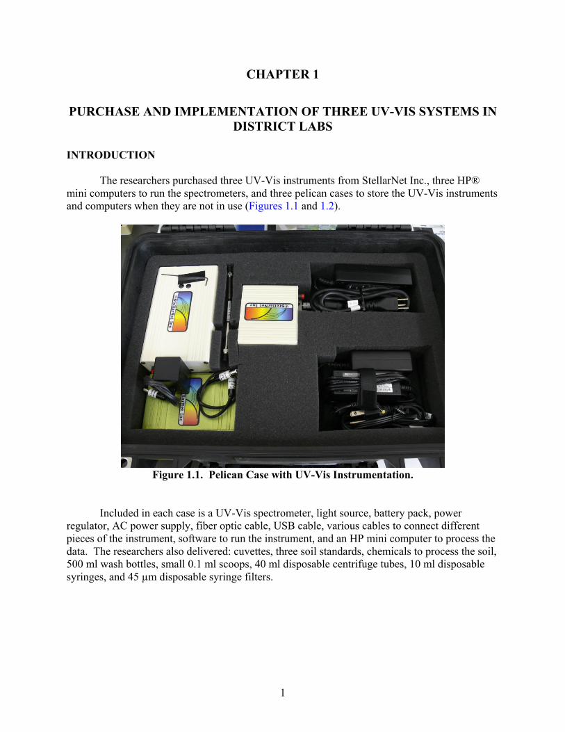
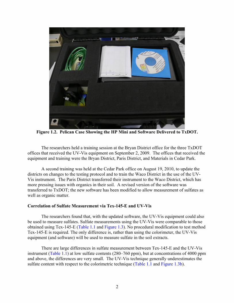
The researchers purchased three UV-Vis instruments from StellarNet Inc., three HP® mini computers to run the spectrometers, and three pelican cases to store the UV-Vis instruments and computers when they are not in use (Figures 1.1 and 1.2).

Figure 1.1. Pelican Case with UV-Vis Instrumentation.

Included in each case is a UV-Vis spectrometer, light source, battery pack, power regulator, AC power supply, fiber optic cable, USB cable, various cables to connect different pieces of the instrument, software to run the instrument, and an HP mini computer to process the data. The researchers also delivered: cuvettes, three soil standards, chemicals to process the soil, 500 ml wash bottles, small 0.1 ml scoops, 40 ml disposable centrifuge tubes, 10 ml disposable syringes, and 45 µm disposable syringe filters.

2

Figure 1.2. Pelican Case Showing the HP Mini and Software Delivered to TxDOT.

The researchers held a training session at the Bryan District office for the three TxDOT offices that received the UV-Vis equipment on September 2, 2009. The offices that received the equipment and training were the Bryan District, Paris District, and Materials in Cedar Park.

A second training was held at the Cedar Park office on August 19, 2010, to update the districts on changes to the testing protocol and to train the Waco District in the use of the UV-Vis instrument. The Paris District transferred their instrument to the Waco District, which has more pressing issues with organics in their soil. A revised version of the software was transferred to TxDOT; the new software has been modified to allow measurement of sulfates as well as organic matter.

Correlation of Sulfate Measurement via Tex-145-E and UV-Vis

The researchers found that, with the updated software, the UV-Vis equipment could also be used to measure sulfates. Sulfate measurements using the UV-Vis were comparable to those obtained using Tex-145-E (Table 1.1 and Figure 1.3). No procedural modification to test method Tex-145-E is required. The only difference is, rather than using the colorimeter, the UV-Vis equipment (and software) will be used to measure sulfate in the soil extracts.

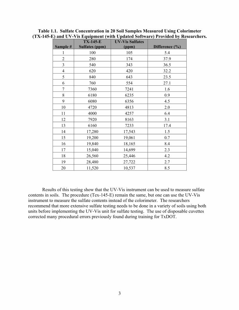
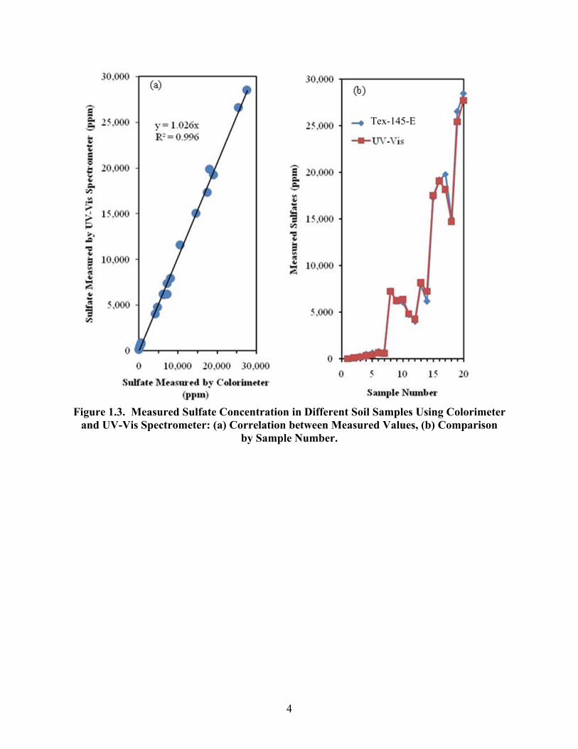
There are large differences in sulfate measurement between Tex-145-E and the UV-Vis instrument (Table 1.1) at low sulfate contents (280–760 ppm), but at concentrations of 4000 ppm and above, the differences are very small. The UV-Vis technique generally underestimates the sulfate content with respect to the colorimetric technique (Table 1.1 and Figure 1.3b).

3

Table 1.1. Sulfate Concentration in 20 Soil Samples Measured Using Colorimeter (TX-145-E) and UV-Vis Equipment (with Updated Software) Provided by Researchers.

Sample #TX-145-E

Sulfates (ppm) UV-Vis Sulfates

(ppm) Difference (%) 1 100 105 5.4 2 280 174 37.9 3 540 343 36.5 4 620 420 32.2 5 840 643 23.5 6 760 554 27.1 7 7360 7241 1.6 8 6180 6235 0.9 9 6080 6356 4.5

10 4720 4813 2.0 11 4000 4257 6.4 12 7920 8163 3.1 13 6160 7233 17.4 14 17,280 17,543 1.5 15 19,200 19,061 0.7 16 19,840 18,165 8.4 17 15,040 14,699 2.3 18 26,560 25,446 4.2 19 28,480 27,722 2.7 20 11,520 10,537 8.5

Results of this testing show that the UV-Vis instrument can be used to measure sulfate contents in soils. The procedure (Tex-145-E) remain the same, but one can use the UV-Vis instrument to measure the sulfate contents instead of the colorimeter. The researchers recommend that more extensive sulfate testing needs to be done in a variety of soils using both units before implementing the UV-Vis unit for sulfate testing. The use of disposable cuvettes corrected many procedural errors previously found during training for TxDOT.

4

Figure 1.3. Measured Sulfate Concentration in Different Soil Samples Using Colorimeter

and UV-Vis Spectrometer: (a) Correlation between Measured Values, (b) Comparison by Sample Number.

Tex-145-E

5

CHAPTER 2 REPEATABILITY STUDIES WITH THE UV-VIS EQUIPMENT

INTRODUCTION

TxDOT Research Project 0-5540 developed a test method to determine soil organic matter (SOM) using UV-Vis spectrophotometry. After development of this test method, Texas Transportation Institute (TTI) initiated efforts to evaluate the precision of the method using two techniques. In the first technique, the amount of soil required for the test is not measured but is instead obtained by using a spoon that is intended to generate 0.1 g of soil. In the second method, the required amount of sample is directly weighed with an analytical balance. DATA COLLECTION METHODS

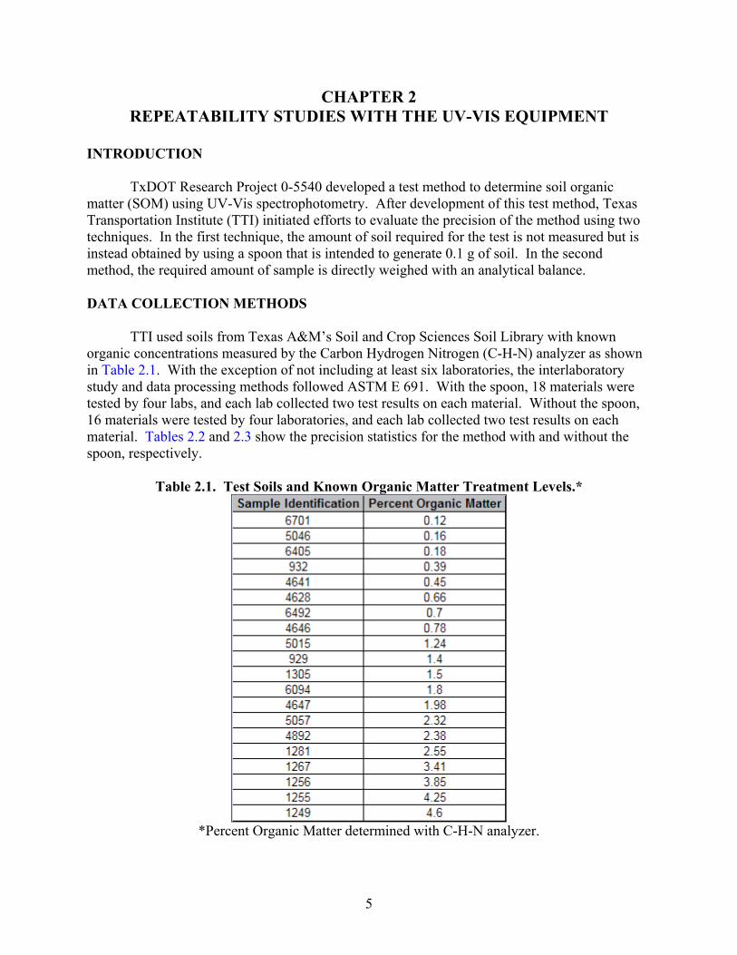
TTI used soils from Texas A&M’s Soil and Crop Sciences Soil Library with known organic concentrations measured by the Carbon Hydrogen Nitrogen (C-H-N) analyzer as shown in Table 2.1. With the exception of not including at least six laboratories, the interlaboratory study and data processing methods followed ASTM E 691. With the spoon, 18 materials were tested by four labs, and each lab collected two test results on each material. Without the spoon, 16 materials were tested by four laboratories, and each lab collected two test results on each material. Tables 2.2 and 2.3 show the precision statistics for the method with and without the spoon, respectively.

Table 2.1. Test Soils and Known Organic Matter Treatment Levels.*

*Percent Organic Matter determined with C-H-N analyzer.

6

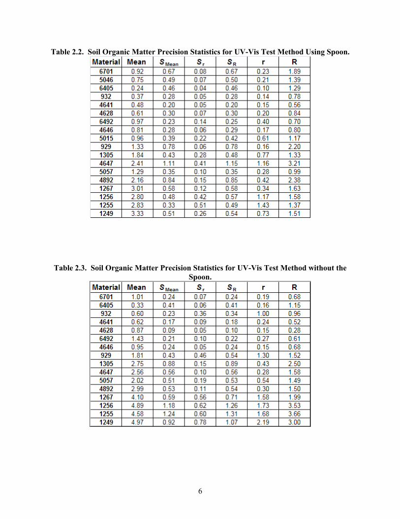
Table 2.2. Soil Organic Matter Precision Statistics for UV-Vis Test Method Using Spoon.

Table 2.3. Soil Organic Matter Precision Statistics for UV-Vis Test Method without the Spoon.

7

DISCUSSION OF RESULTS The interlaboratory study results allow for investigation of two important topics:

• Does either method provide better precision?

• Is there a difference in accuracy among the methods?

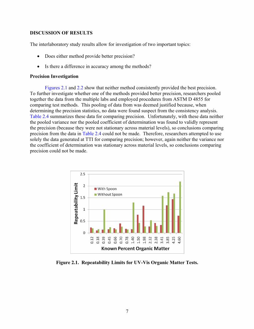
Precision Investigation

Figures 2.1 and 2.2 show that neither method consistently provided the best precision. To further investigate whether one of the methods provided better precision, researchers pooled together the data from the multiple labs and employed procedures from ASTM D 4855 for comparing test methods. This pooling of data from was deemed justified because, when determining the precision statistics, no data were found suspect from the consistency analysis. Table 2.4 summarizes these data for comparing precision. Unfortunately, with these data neither the pooled variance nor the pooled coefficient of determination was found to validly represent the precision (because they were not stationary across material levels), so conclusions comparing precision from the data in Table 2.4 could not be made. Therefore, researchers attempted to use solely the data generated at TTI for comparing precision; however, again neither the variance nor the coefficient of determination was stationary across material levels, so conclusions comparing precision could not be made.

Figure 2.1. Repeatability Limits for UV-Vis Organic Matter Tests.

8

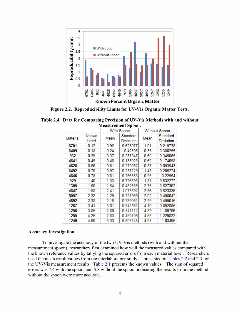
Figure 2.2. Reproducibility Limits for UV-Vis Organic Matter Tests.

Table 2.4. Data for Comparing Precision of UV-Vis Methods with and without

Measurement Spoon.

Accuracy Investigation

To investigate the accuracy of the two UV-Vis methods (with and without the measurement spoon), researchers first examined how well the measured values compared with the known reference values by tallying the squared errors from each material level. Researchers used the mean result values from the interlaboratory study as presented in Tables 2.2 and 2.3 for the UV-Vis measurement results. Table 2.1 presents the known values. The sum of squared errors was 7.4 with the spoon, and 5.8 without the spoon, indicating the results from the method without the spoon were more accurate.

9

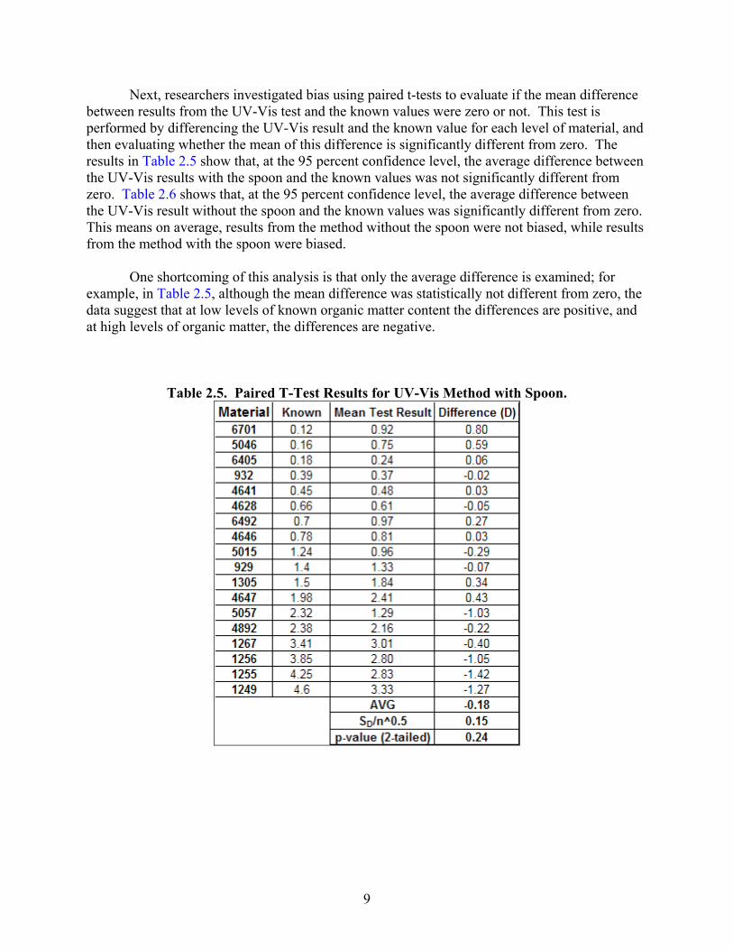
Next, researchers investigated bias using paired t-tests to evaluate if the mean difference between results from the UV-Vis test and the known values were zero or not. This test is performed by differencing the UV-Vis result and the known value for each level of material, and then evaluating whether the mean of this difference is significantly different from zero. The results in Table 2.5 show that, at the 95 percent confidence level, the average difference between the UV-Vis results with the spoon and the known values was not significantly different from zero. Table 2.6 shows that, at the 95 percent confidence level, the average difference between the UV-Vis result without the spoon and the known values was significantly different from zero. This means on average, results from the method without the spoon were not biased, while results from the method with the spoon were biased.

One shortcoming of this analysis is that only the average difference is examined; for example, in Table 2.5, although the mean difference was statistically not different from zero, the data suggest that at low levels of known organic matter content the differences are positive, and at high levels of organic matter, the differences are negative.

Table 2.5. Paired T-Test Results for UV-Vis Method with Spoon.

10

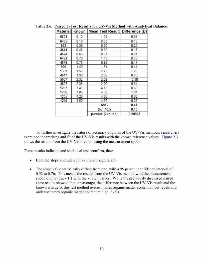
Table 2.6. Paired T-Test Results for UV-Vis Method with Analytical Balance.

To further investigate the nature of accuracy and bias of the UV-Vis methods, researchers examined the tracking and fit of the UV-Vis results with the known reference values. Figure 2.3 shows the results from the UV-Vis method using the measurement spoon. These results indicate, and statistical tests confirm, that:

• Both the slope and intercept values are significant.

• The slope value statistically differs from one, with a 95 percent confidence interval of 0.52 to 0.76. This means the results from the UV-Vis method with the measurement spoon did not track 1:1 with the known values. While the previously discussed paired t-test results showed that, on average, the difference between the UV-Vis result and the known was zero, this test method overestimates organic matter content at low levels and underestimates organic matter content at high levels.

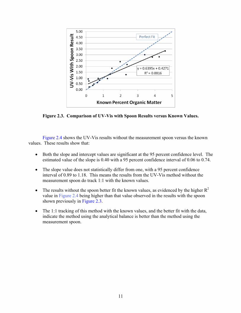
11

Figure 2.3. Comparison of UV-Vis with Spoon Results versus Known Values.

Figure 2.4 shows the UV-Vis results without the measurement spoon versus the known values. These results show that:

• Both the slope and intercept values are significant at the 95 percent confidence level. The

estimated value of the slope is 0.40 with a 95 percent confidence interval of 0.06 to 0.74.

• The slope value does not statistically differ from one, with a 95 percent confidence interval of 0.89 to 1.18. This means the results from the UV-Vis method without the measurement spoon do track 1:1 with the known values.

• The results without the spoon better fit the known values, as evidenced by the higher R2 value in Figure 2.4 being higher than that value observed in the results with the spoon shown previously in Figure 2.3.

• The 1:1 tracking of this method with the known values, and the better fit with the data, indicate the method using the analytical balance is better than the method using the measurement spoon.

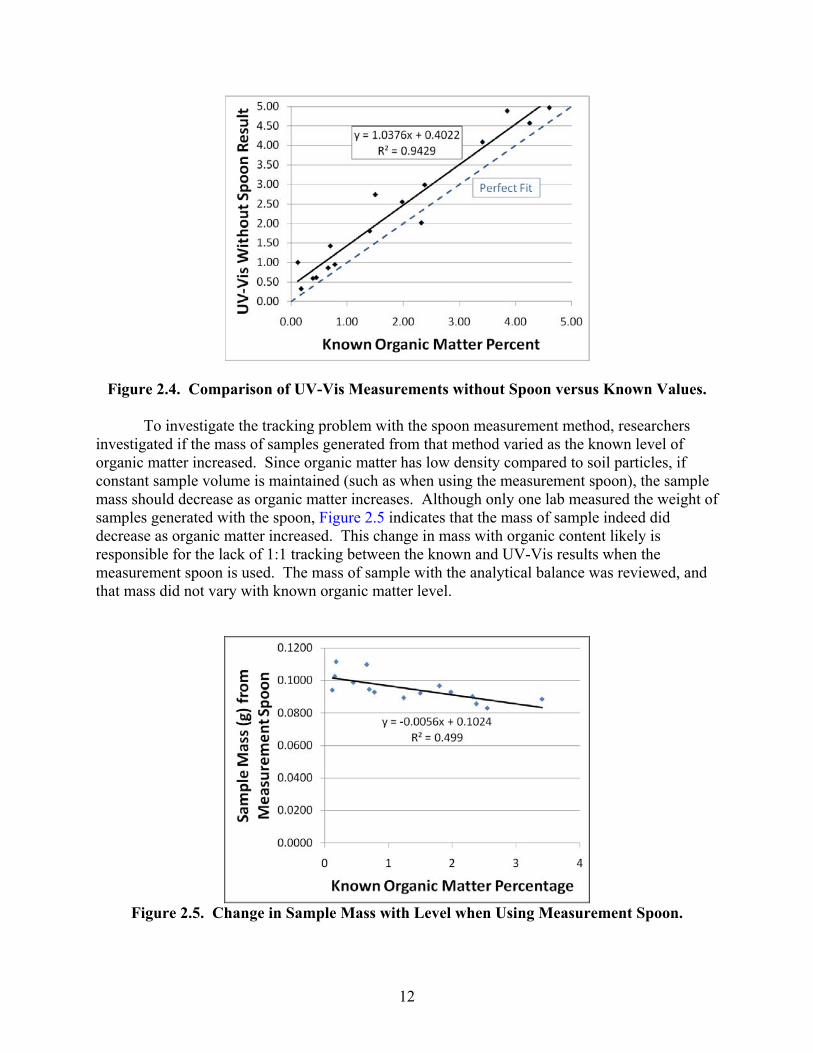
12

Figure 2.4. Comparison of UV-Vis Measurements without Spoon versus Known Values.

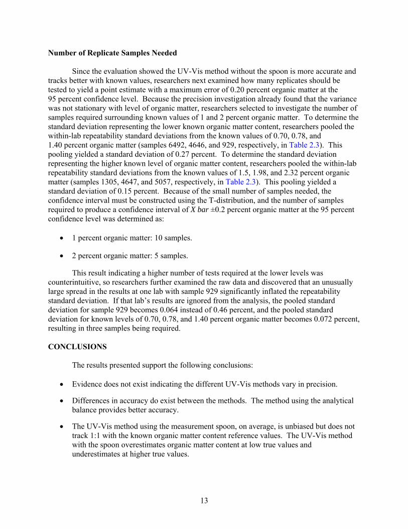
To investigate the tracking problem with the spoon measurement method, researchers investigated if the mass of samples generated from that method varied as the known level of organic matter increased. Since organic matter has low density compared to soil particles, if constant sample volume is maintained (such as when using the measurement spoon), the sample mass should decrease as organic matter increases. Although only one lab measured the weight of samples generated with the spoon, Figure 2.5 indicates that the mass of sample indeed did decrease as organic matter increased. This change in mass with organic content likely is responsible for the lack of 1:1 tracking between the known and UV-Vis results when the measurement spoon is used. The mass of sample with the analytical balance was reviewed, and that mass did not vary with known organic matter level.

Figure 2.5. Change in Sample Mass with Level when Using Measurement Spoon.

13

Number of Replicate Samples Needed

Since the evaluation showed the UV-Vis method without the spoon is more accurate and tracks better with known values, researchers next examined how many replicates should be tested to yield a point estimate with a maximum error of 0.20 percent organic matter at the 95 percent confidence level. Because the precision investigation already found that the variance was not stationary with level of organic matter, researchers selected to investigate the number of samples required surrounding known values of 1 and 2 percent organic matter. To determine the standard deviation representing the lower known organic matter content, researchers pooled the within-lab repeatability standard deviations from the known values of 0.70, 0.78, and 1.40 percent organic matter (samples 6492, 4646, and 929, respectively, in Table 2.3). This pooling yielded a standard deviation of 0.27 percent. To determine the standard deviation representing the higher known level of organic matter content, researchers pooled the within-lab repeatability standard deviations from the known values of 1.5, 1.98, and 2.32 percent organic matter (samples 1305, 4647, and 5057, respectively, in Table 2.3). This pooling yielded a standard deviation of 0.15 percent. Because of the small number of samples needed, the confidence interval must be constructed using the T-distribution, and the number of samples required to produce a confidence interval of X bar ±0.2 percent organic matter at the 95 percent confidence level was determined as:

• 1 percent organic matter: 10 samples.

• 2 percent organic matter: 5 samples.

This result indicating a higher number of tests required at the lower levels was counterintuitive, so researchers further examined the raw data and discovered that an unusually large spread in the results at one lab with sample 929 significantly inflated the repeatability standard deviation. If that lab’s results are ignored from the analysis, the pooled standard deviation for sample 929 becomes 0.064 instead of 0.46 percent, and the pooled standard deviation for known levels of 0.70, 0.78, and 1.40 percent organic matter becomes 0.072 percent, resulting in three samples being required. CONCLUSIONS

The results presented support the following conclusions:

• Evidence does not exist indicating the different UV-Vis methods vary in precision.

• Differences in accuracy do exist between the methods. The method using the analytical balance provides better accuracy.

• The UV-Vis method using the measurement spoon, on average, is unbiased but does not track 1:1 with the known organic matter content reference values. The UV-Vis method with the spoon overestimates organic matter content at low true values and underestimates at higher true values.

14

• Results from the UV-Vis method using an analytical balance to obtain the required quantity of sample do track 1:1 with the known values but exhibit some bias.

• The UV-Vis method with the analytical balance should be used if the desire is to obtain a test result as accurate as possible. The UV-Vis result should be reduced by 0.4 to account for bias and produce an estimate of the true organic matter percentage that would be obtained with a C-H-N analyzer. Results from the interlaboratory study indicate this approach would provide an organic content measurement with an accuracy of ±0.21 percent organic matter.

o To provide a test result with a maximum error (at the 95 percent confidence level) of 0.20 percent organic matter, three replicate tests should be conducted and averaged. Testing in this manner means that, 95 percent of the time, the true sample mean will be within 0.20 percent organic matter of the test result.

• In context of the TxDOT goal to rapidly screen for organics in the field, the UV-Vis method with the spoon should be an acceptable field screening method. This method tends to overestimate organic matter content and, thus, will be conservative.

• Consideration should be given to a two-part TxDOT test method. One part would be for a field screening test using the spoon, where if the test result exceeds 1 percent organic matter content, further investigation of the soils compatibility with stabilization is needed. The second part would be a laboratory test using an analytical balance to obtain the sample size.

15

CHAPTER 3 FIELD AND LAB TESTING

INTRODUCTION

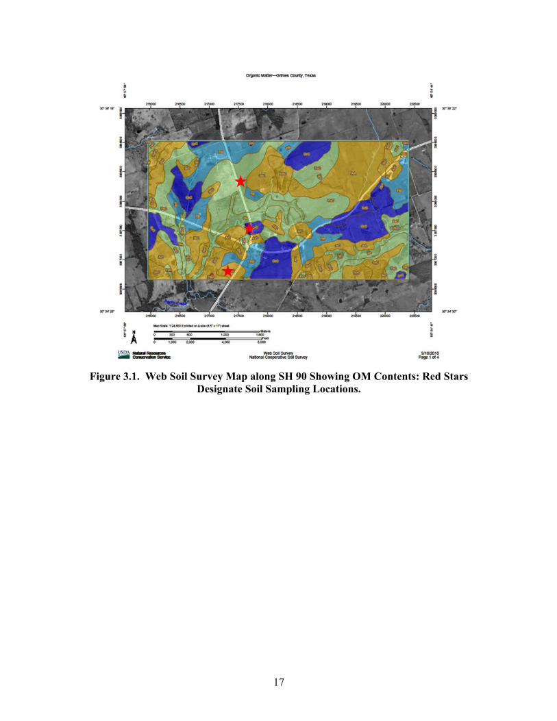
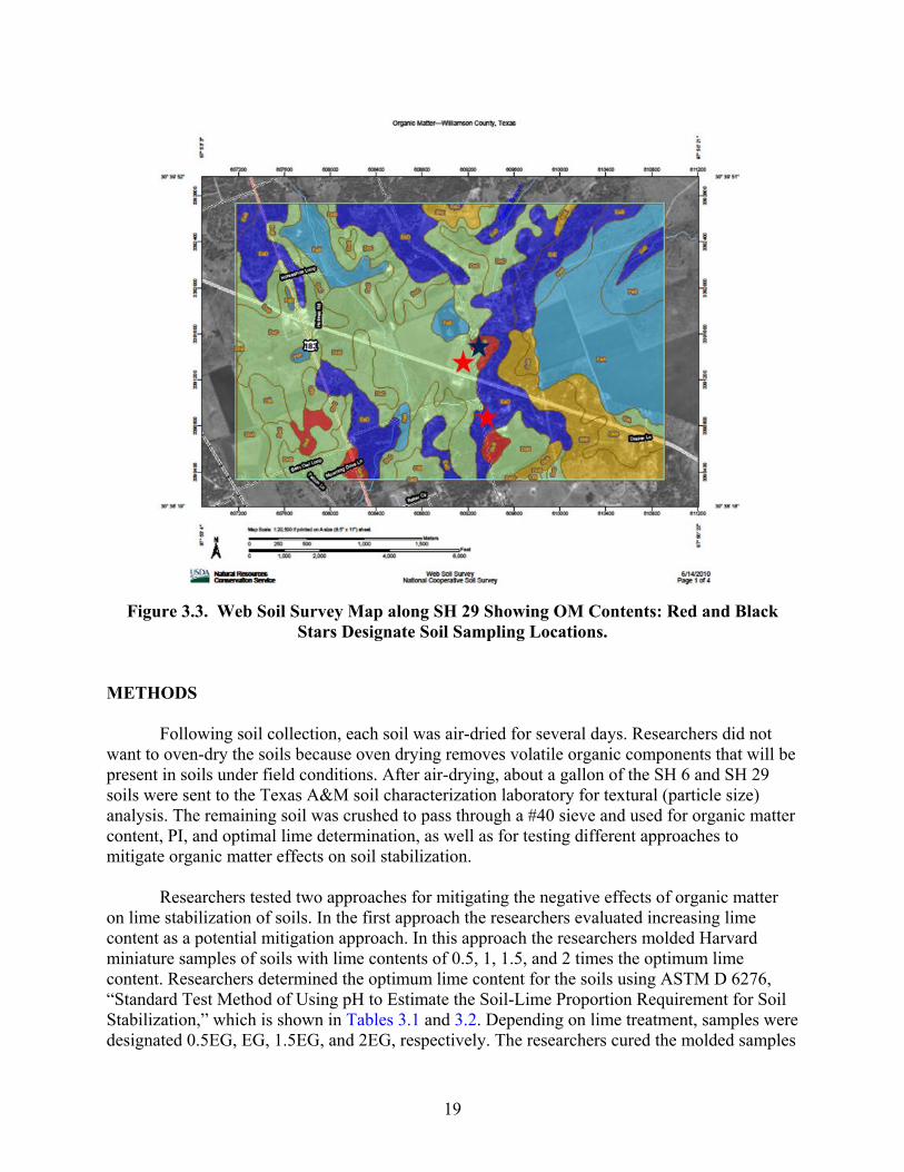
To determine what organic contents are problematic in Texas soils and potential remediation techniques, the researchers selected soils from the Bryan, Waco, and Austin Districts. Each of these districts has reported problems with organics in soil stabilization projects. Soils representing a wide range of properties were targeted. The researchers utilized the Web Soil Survey (WSS) in identifying suitable study sites and preselecting potential sampling locations. Researchers selected three study sites (SH 90, SH 6 and SH 29) and nine sampling locations (three per study site). Maps for each study site and soil sampling locations are shown in Figures 3.1, 3.2, and 3.3. The SH 90 location is just north of SH 30 at the community of Roans Prairie in the Bryan District. The SH 6 location is located in the Waco District just south of the town of Riesel, and the SH 29 location is about 1500 m east of the intersection with US 183 close to the town of Liberty Hill in the Austin District.

Selection of the sampling locations at each study site was largely based on the following soil properties:

• PI (the need for moderate to high plasticity because lime would not be used to stabilize

low plasticity soils).

• OM (low, medium, and high organic contents).

• pH (acidic, neutral, and alkaline pH soils).

A handheld GPS unit was used to find and verify the preselected sampling locations on the maps. Soils were collected from the top 2 ft at each location. Table 3.1 shows the percent organic matter, the pH, and the Soil Series determined using the WSS maps. Researchers have also included the plasticity index and lime percentages measured with the Eades and Grim method.

Table 3.1. Properties Reported from the WSS along with Engineering Properties of Soils Used in This Study.

Sample Location WSS OM (%) PI E&G Lime (%) pH Soil SeriesSH 90 0.58-0.75 14 5 5.1-5.5 Shiro lmy fn sd

0.75-0.9 19 5 4.5-5 Falba fn sdy lm1.27-2.42 21 4 6.6-7.3 Flatonia cly lm

SH 6 <0.76 23 4 7 Crockett sdy lm0.96-1.25 24 4.5 6.7 Wilson cly lm

2-2.5 23 5 7.5 Gowen cly lmSH 29 <0.94 20 2 7 Georgetown cly lm

1.5-2.0 33 4 8.2 Denton slty cly2.5-6.5 24 2 7.5 Eckrant cobbly cly

16

The researchers wanted to compare the data obtained with the WSS to laboratory measured data from actual field samples. Researchers have full textural information for two of the three locations; for the SH 90 location, textural data were not collected. Researchers found that, in most cases, representative values provided by the WSS for the different soil properties were inconsistent with measured values (Table 3.2). However, as shown in Table 3.2, variability in the measured soil properties was sufficient to facilitate a comprehensive study. For example, the range of organic matter content in the soils was between 1 and 6 percent, which covers the typical range for Texas soils. Similarly, plasticity index of the soils ranges from a low of 14 to a high of 33, which is in the range for lime stabilization.

Table 3.2. Physical and Chemical Properties of Soils Selected to Measure Effects of Organic Matter on Stabilization.

SH 6 SH 29 SH 90 1 2 3 1 2 3 1 2 3

Calcareous? Yes Yes Yes Yes Yes Yes No No No Plasticity limit 23 24 23 20 33 24 14 19 21 Sand (%) 40.2 47.0 34.6 20.0 7.80 15.8 Silt (%) 21.7 24.3 29.4 54.4 44.5 46.1 Clay (%) 38.1 28.7 36 25.6 47.7 38.1

Textural Class

Clay loam

Sandy clay loam

Clay loam

Silt loam

Silt Clay

Silty Clay loam

pH 7.9 7.9 8.1 7.8 7.6 7.7

CEC (cmol kg-1) 30.2 28.8 34.6 32.3 57.8 50.2 Organic Matter (%) 1.1 1.9 2.2 2.6 5.7 5.9 1.2 1.8 1.4

Optimal Lime, EG (%) 4 4.5 5 2 4 2 5 5 4

The data obtained with this research suggest that the WSS is a good tool to obtain general

trends in soil properties. However, the resolution of the mapping is not good enough to distinguish high and low organic contents and textural classes with accuracy on the scale of a few hundred feet.

17

Figure 3.1. Web Soil Survey Map along SH 90 Showing OM Contents: Red Stars

Designate Soil Sampling Locations.

18

Figure 3.2. Web Soil Survey Map along SH 6 Showing OM Contents: Red and Black Stars

Designate Soil Sampling Locations.

19

Figure 3.3. Web Soil Survey Map along SH 29 Showing OM Contents: Red and Black

Stars Designate Soil Sampling Locations.

METHODS

Following soil collection, each soil was air-dried for several days. Researchers did not want to oven-dry the soils because oven drying removes volatile organic components that will be present in soils under field conditions. After air-drying, about a gallon of the SH 6 and SH 29 soils were sent to the Texas A&M soil characterization laboratory for textural (particle size) analysis. The remaining soil was crushed to pass through a #40 sieve and used for organic matter content, PI, and optimal lime determination, as well as for testing different approaches to mitigate organic matter effects on soil stabilization.

Researchers tested two approaches for mitigating the negative effects of organic matter on lime stabilization of soils. In the first approach the researchers evaluated increasing lime content as a potential mitigation approach. In this approach the researchers molded Harvard miniature samples of soils with lime contents of 0.5, 1, 1.5, and 2 times the optimum lime content. Researchers determined the optimum lime content for the soils using ASTM D 6276, “Standard Test Method of Using pH to Estimate the Soil-Lime Proportion Requirement for Soil Stabilization,” which is shown in Tables 3.1 and 3.2. Depending on lime treatment, samples were designated 0.5EG, EG, 1.5EG, and 2EG, respectively. The researchers cured the molded samples

20

at 100 percent humidity and 23°C for 28 days, prior to measuring the unconfined compressive strength.

In the second mitigation approach, researchers evaluated soluble Ca2+ as a potential

additive to the stabilizer mix. In this approach, samples were prepared, cured, and tested as in approach 1 except that in addition to the lime, calcium chloride dihydrate salt (CaCl2.2H2O) was added to the mix at a rate of 0.25 times the optimum lime content. For example, a sample with an optimum lime content of 4 percent by weight would receive 4 percent hydrated lime and 1 percent calcium chloride dihydrate. Samples containing CaCl2.2H2O as an additive were designated 0.5EG-Ca, EG-Ca, 1.5EG-Ca, and 2EG-Ca. All samples in approaches 1 and 2 were molded in duplicate to a dry bulk density of 1.6 g cm-3 and moisture content of 16–18 percent by weight.

Following the 28 day moist cure, the unconfined compressive strength (UCS) measurements were made using an Instron Universal Testing system run at a rate of 0.05 in/min. Based on UCS results and soil chemistry, the researchers selected specific samples to run on a SDT Q600 heat-flow Differential Scanning Calorimeter (DSC) to determine if pozzolanic reaction products were being formed and what those products may be. Researchers pulverized the samples with an agate mortar and pestle and sieved the samples through a #325 sieve. Researchers placed approximately 30 mg of sample in a ceramic crucible and ran the DSC from 23 to 1050°C at a ramp rate of 10°C/min. RESULTS

As stated before, the researchers tested 144 Harvard miniature samples for UCS using two different mitigation techniques (higher lime contents and calcium chloride) to treat the soils with high organic matter: the organic contents ranged from 1.1 to 5.9 percent. The samples selected to run in the DSC include: SH 6-1 (EG, 2EG, EG-Ca, 2EG-Ca), SH 29-2 (EG, 2EG, EG-Ca, 2EG-Ca), SH 29-3 (EG, 2EG, EG-Ca, 2EG-Ca), and SH 90-3 (0.5EG, EG, 2EG, 0.5EG-Ca, EG-Ca, 2EG-Ca). Unconfined Compressive Strength Results

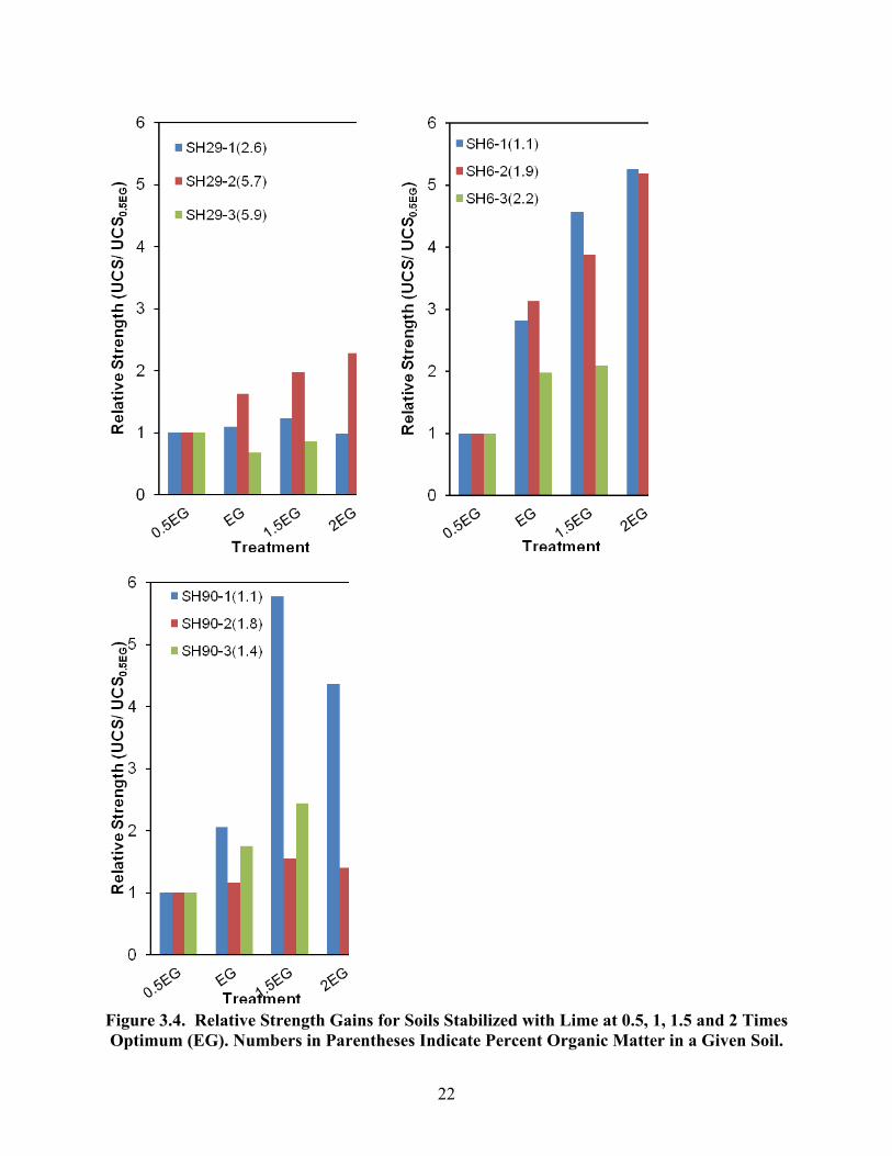
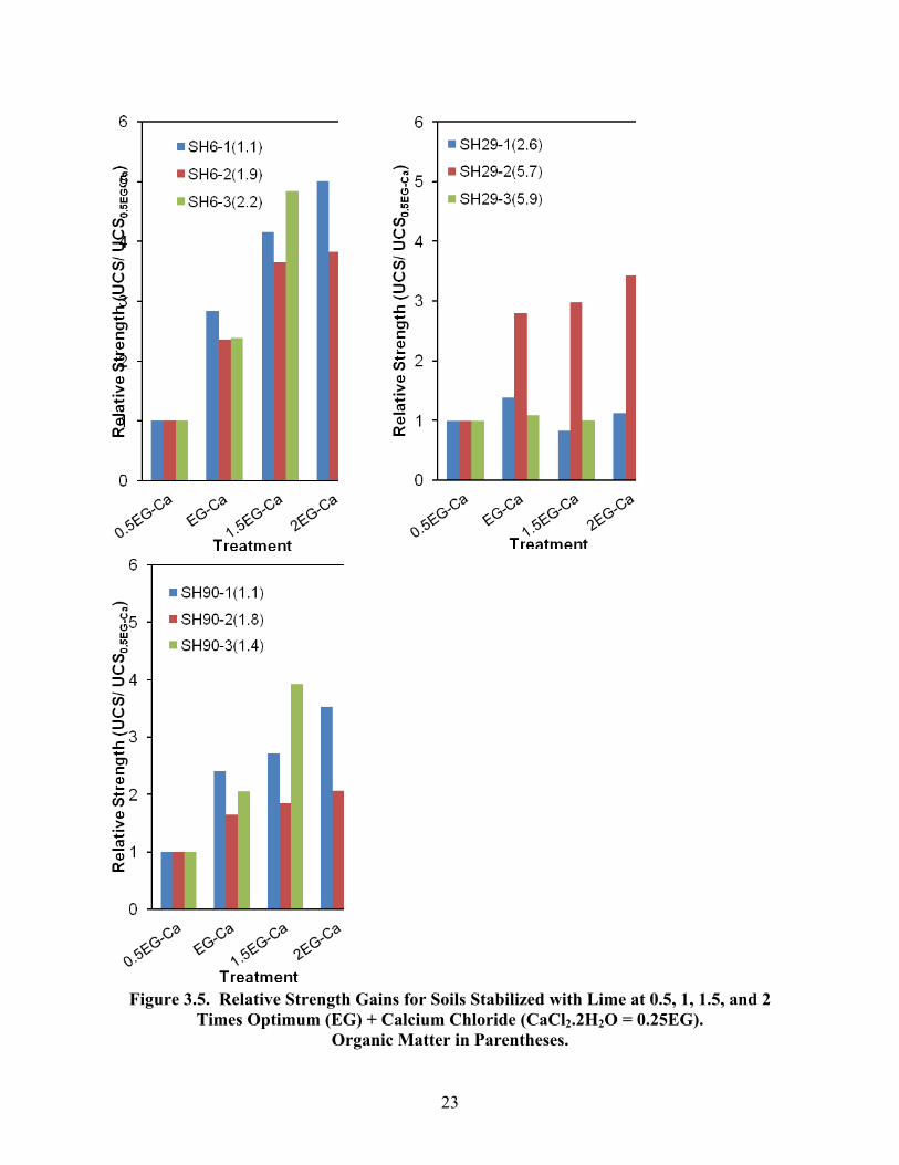
Table 3.3 shows unconfined compressive strength data for the molded samples (after moist curing for 28 days): each reported UCS value is an average of two samples. Evidence for improved stabilization was apparent for both mitigation approaches in all but two (SH 29-1 and SH 29-3) of the nine soils tested. However, the relative improvement in stabilization for a given treatment varied greatly across soils. For example, increasing lime content from optimum (EG) to 2 times optimum (2EG) resulted in a strength gain of 80 percent for SH 6-1 compared to 60 and 20 percent for SH 6-2 and SH 6-3, respectively (Figure 3.4). For these same soils and lime treatments, the addition of CaCl2.2H2O improved the strength of SH 6-3 by 105 percent but had no additional effect on SH 6-1 and SH 6-2 compared to lime alone (Figure 3.5). That is, for SH 6-3, 2EG-Ca/EG-Ca >> 2EG/EG; while for SH 6-1 and SH 6-2, 2EG-Ca/EG-Ca ≈ 2EG/EG.

Variable effects of adding CaCl2.2H2O (at a rate of 0.25EG) on stabilization were also apparent in the other soils. For SH 90-3, 2EG-Ca/EG-Ca was significantly greater than 2EG/EG

21

consistent with improved stabilization over lime only. However, the addition of CaCl2.2H2O had no apparent effect on stabilization of SH 90-2 (2EG-Ca/EG-Ca ≈ 2EG/EG) but appeared to negatively impact the stabilization of SH 90-1 and SH 29-2 (2EG-Ca/EG-Ca << 2EG/EG).

Table 3.3. Unconfined Compressive Strengths for 28 Day Cured Samples Treated Using Mitigation Approach 1 [Lime at a Rate of 0.5, 1, 1.5, or 2 Times Optimal Content (EG)] and Mitigation Approach 2 [Mitigation Approach 1 + Calcium Chloride Dihydrate Salt

(CaCl2.2H2O = 0.25EG)]. Values Are Average Values for Duplicate Samples. Mitigation Approach 1 Mitigation Approach 2

0.5EG EG 1.5EG 2EG 0.5EG-Ca EG-Ca 1.5EG-Ca 2EG-Ca Sample --------------UCS (psi)------------------ ----------------UCS (psi)---------------------- SH 6-1 21.2 59.7 96.7 111 19.1 54.0 79.2 95.9 SH 6-2 13.7 43.0 53.3 71.2 19.8 46.7 72.0 75.6 SH 6-3 49.8 98.4 104 120 35.5 84.6 172 174

SH 29-1 42.3 46.1 51.9 41.5 22.9 32.0 19.2 25.9 SH 29-2 116 189 229 264 60.3 169 180 207 SH 29-3 62.9 42.1 53.5 65 31.8 34.6 32.2 19.2

SH 90-1 29.3 60.2 169 128 51.6 125 141 182 SH 90-2 74.8 87.0 116 105 78.0 129 144 162 SH 90-3 31.7 55.3 77.2 95.1 32.1 65.9 126 136

22

Figure 3.4. Relative Strength Gains for Soils Stabilized with Lime at 0.5, 1, 1.5 and 2 Times Optimum (EG). Numbers in Parentheses Indicate Percent Organic Matter in a Given Soil.

23

Figure 3.5. Relative Strength Gains for Soils Stabilized with Lime at 0.5, 1, 1.5, and 2

Times Optimum (EG) + Calcium Chloride (CaCl2.2H2O = 0.25EG). Organic Matter in Parentheses.

24

Differential Scanning Calorimetry Results

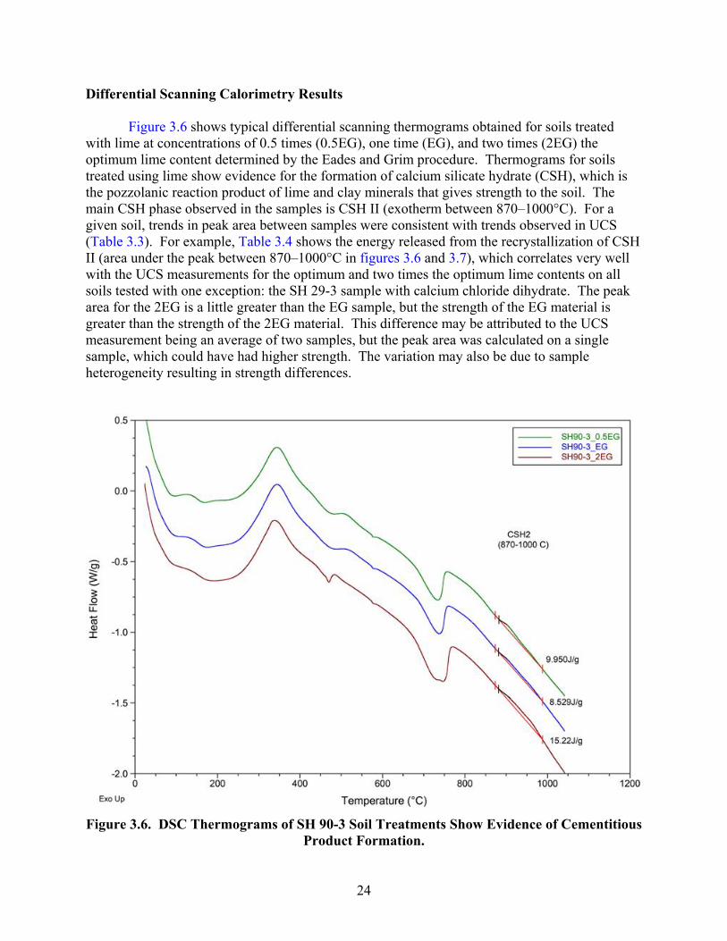
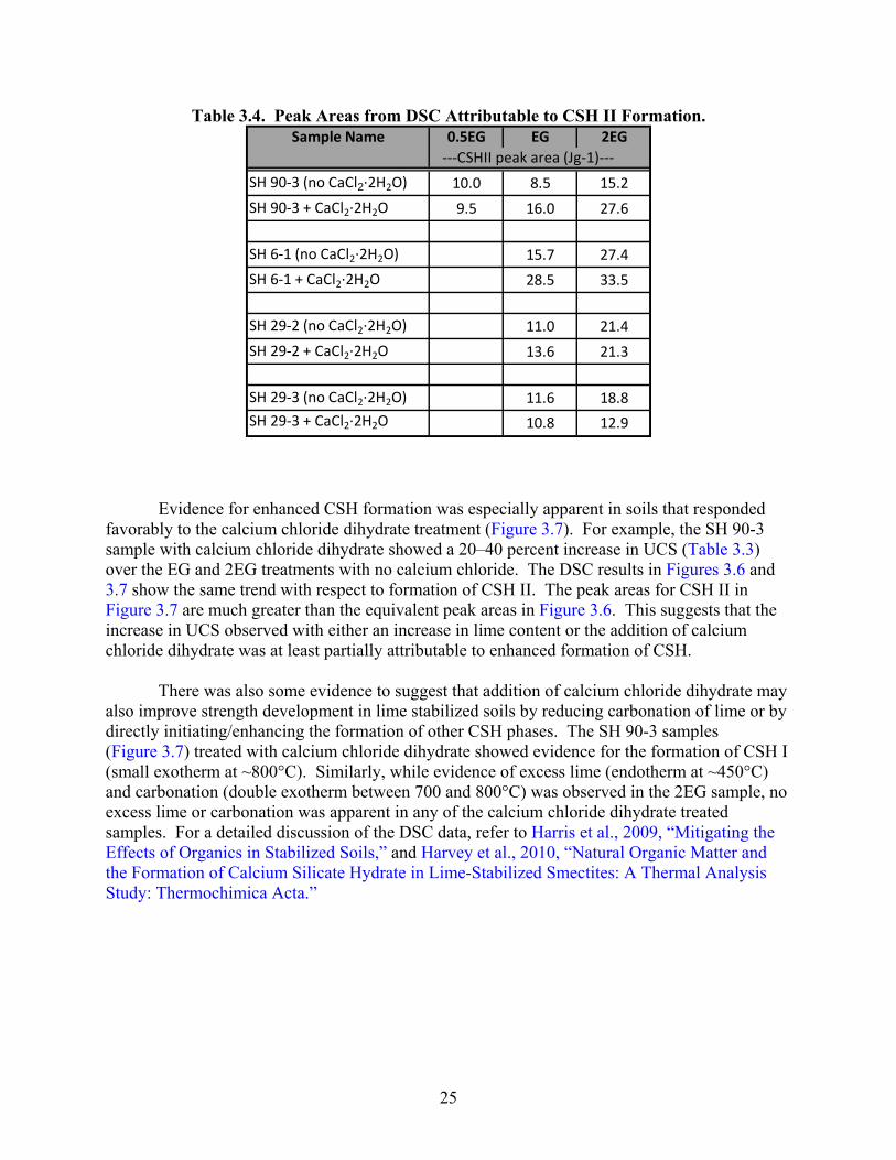
Figure 3.6 shows typical differential scanning thermograms obtained for soils treated with lime at concentrations of 0.5 times (0.5EG), one time (EG), and two times (2EG) the optimum lime content determined by the Eades and Grim procedure. Thermograms for soils treated using lime show evidence for the formation of calcium silicate hydrate (CSH), which is the pozzolanic reaction product of lime and clay minerals that gives strength to the soil. The main CSH phase observed in the samples is CSH II (exotherm between 870–1000°C). For a given soil, trends in peak area between samples were consistent with trends observed in UCS (Table 3.3). For example, Table 3.4 shows the energy released from the recrystallization of CSH II (area under the peak between 870–1000°C in figures 3.6 and 3.7), which correlates very well with the UCS measurements for the optimum and two times the optimum lime contents on all soils tested with one exception: the SH 29-3 sample with calcium chloride dihydrate. The peak area for the 2EG is a little greater than the EG sample, but the strength of the EG material is greater than the strength of the 2EG material. This difference may be attributed to the UCS measurement being an average of two samples, but the peak area was calculated on a single sample, which could have had higher strength. The variation may also be due to sample heterogeneity resulting in strength differences.

Figure 3.6. DSC Thermograms of SH 90-3 Soil Treatments Show Evidence of Cementitious

Product Formation.

25

Table 3.4. Peak Areas from DSC Attributable to CSH II Formation. Sample Name 0.5EG EG 2EG

‐‐‐CSHII peak area (Jg‐1)‐‐‐

SH 90‐3 (no CaCl2∙2H2O) 10.0 8.5 15.2

SH 90‐3 + CaCl2∙2H2O 9.5 16.0 27.6

SH 6‐1 (no CaCl2∙2H2O) 15.7 27.4

SH 6‐1 + CaCl2∙2H2O 28.5 33.5

SH 29‐2 (no CaCl2∙2H2O) 11.0 21.4

SH 29‐2 + CaCl2∙2H2O 13.6 21.3

SH 29‐3 (no CaCl2∙2H2O) 11.6 18.8SH 29‐3 + CaCl2∙2H2O 10.8 12.9

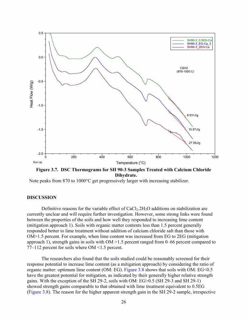
Evidence for enhanced CSH formation was especially apparent in soils that responded favorably to the calcium chloride dihydrate treatment (Figure 3.7). For example, the SH 90-3 sample with calcium chloride dihydrate showed a 20–40 percent increase in UCS (Table 3.3) over the EG and 2EG treatments with no calcium chloride. The DSC results in Figures 3.6 and 3.7 show the same trend with respect to formation of CSH II. The peak areas for CSH II in Figure 3.7 are much greater than the equivalent peak areas in Figure 3.6. This suggests that the increase in UCS observed with either an increase in lime content or the addition of calcium chloride dihydrate was at least partially attributable to enhanced formation of CSH.

There was also some evidence to suggest that addition of calcium chloride dihydrate may also improve strength development in lime stabilized soils by reducing carbonation of lime or by directly initiating/enhancing the formation of other CSH phases. The SH 90-3 samples (Figure 3.7) treated with calcium chloride dihydrate showed evidence for the formation of CSH I (small exotherm at ~800°C). Similarly, while evidence of excess lime (endotherm at ~450°C) and carbonation (double exotherm between 700 and 800°C) was observed in the 2EG sample, no excess lime or carbonation was apparent in any of the calcium chloride dihydrate treated samples. For a detailed discussion of the DSC data, refer to Harris et al., 2009, “Mitigating the Effects of Organics in Stabilized Soils,” and Harvey et al., 2010, “Natural Organic Matter and the Formation of Calcium Silicate Hydrate in Lime-Stabilized Smectites: A Thermal Analysis Study: Thermochimica Acta.”

26

Figure 3.7. DSC Thermograms for SH 90-3 Samples Treated with Calcium Chloride

Dihydrate. Note peaks from 870 to 1000°C get progressively larger with increasing stabilizer.

DISCUSSION

Definitive reasons for the variable effect of CaCl2.2H2O additions on stabilization are currently unclear and will require further investigation. However, some strong links were found between the properties of the soils and how well they responded to increasing lime content (mitigation approach 1). Soils with organic matter contents less than 1.5 percent generally responded better to lime treatment without addition of calcium chloride salt than those with OM>1.5 percent. For example, when lime content was increased from EG to 2EG (mitigation approach 1), strength gains in soils with OM >1.5 percent ranged from 0–66 percent compared to 77–112 percent for soils where OM <1.5 percent.

The researchers also found that the soils studied could be reasonably screened for their response potential to increase lime content (as a mitigation approach) by considering the ratio of organic matter: optimum lime content (OM: EG). Figure 3.8 shows that soils with OM: EG<0.5 have the greatest potential for mitigation, as indicated by their generally higher relative strength gains. With the exception of the SH 29-2, soils with OM: EG>0.5 (SH 29-3 and SH 29-1) showed strength gains comparable to that obtained with lime treatment equivalent to 0.5EG (Figure 3.8). The reason for the higher apparent strength gain in the SH 29-2 sample, irrespective

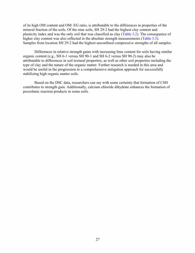
27

of its high OM content and OM: EG ratio, is attributable to the differences in properties of the mineral fraction of the soils. Of the nine soils, SH 29-2 had the highest clay content and plasticity index and was the only soil that was classified as clay (Table 3.2). The consequence of higher clay content was also reflected in the absolute strength measurements (Table 3.3). Samples from location SH 29-2 had the highest unconfined compressive strengths of all samples.

Differences in relative strength gains with increasing lime content for soils having similar organic content (e.g., SH 6-1 versus SH 90-1 and SH 6-2 versus SH 90-2) may also be attributable to differences in soil textural properties, as well as other soil properties including the type of clay and the nature of the organic matter. Further research is needed in this area and would be useful in the progression to a comprehensive mitigation approach for successfully stabilizing high organic matter soils.

Based on the DSC data, researchers can say with some certainty that formation of CSH contributes to strength gain. Additionally, calcium chloride dihydrate enhances the formation of pozzolanic reaction products in some soils.

28

Figure 3.8. Relative Strength Gains as a Function of Organic Matter Content: Optimal

Lime Content (OM: EG) for Soils Treated Using Hydrated Lime Only (0.5EG, EG, 1.5EG, 2EG).

SH29-2

29

CHAPTER 4 TEST PROTOCOL

INTRODUCTION

The researchers developed a testing protocol to follow based on results obtained from this research. Below are some highlights of the revelations made with this research project, remaining questions to be answered, and the recommended testing protocol.

Before this research, researchers commonly believed that the humic acid fraction was detrimental to lime stabilization, and there was no documentation about the effect of lignite on stabilization with lime. This research reveals the order of influence for organic matter adversely affecting lime stabilization with respect to UCS:

Fulvic Acid>Humic Acid>Lignite

Based on DSC and X-ray diffraction (XRD) analyses of samples run in UCS testing, an increase in the organic matter content above 1.5 percent causes decreased strength predominantly due to inhibition of formation of CSH. Previous researchers speculated about causes of strength loss prior to this research.

The researchers determined that the pozzolanic reactions are much more complicated than previously thought. The type of saturating cation affects the pozzolanic reaction products formed. Calcium saturated smectite has a higher strength loss than sodium saturated smectite percentage wise when organic matter is increased in the sample.

The amount of organic matter that affects the strength gain is complicated because the type of organic matter (fulvic acid, humic acid), the cation saturation of the clay/smectite (Ca, Na, Mg, etc.), and the clay type (smectite, kaolinite, etc.) will all affect strength gain by modifying the type and quantity of pozzolanic reaction product formed (CSH I, CSH II, etc.). Higher organic contents generally decrease the amount of pozzolanic reaction product formed (Compare SH 6-1 and SH 90-3 data).

The researchers found for high organic content soils (generally >1 percent SOM) that increasing the lime content above the optimum level (determined by Eades and Grim method) enhances the UCS of some soils and does not help with other soils. Alternatively, addition of calcium chloride salt seems to remediate some natural soils with SOM contents above 1.5 percent by forming more pozzolanic reaction products. RESEARCH QUESTIONS Does lime leach out of soil after stabilization products are formed? Does the organic matter leach the lime out of the soil? What is the percentage of pozzolanic reaction product that is needed for permanent stabilization?

30

How much is needed and how does calcium chloride affect lime stabilization reactions? Does the soil texture affect the critical organic matter to optimum lime content ratio for successful stabilization? For example, one soil analyzed from SH 29 was a clay soil; the other soils were all loams. The clay soil plotted differently from all of the loam soils; it had much higher strengths than the other soils even with very high OM contents. Can calcium chloride be mixed with the lime, or do they have to be mixed separately in the soil? Is there a mellowing time that is optimal for use of calcium chloride? How do high organic matter soils with different mineralogical constituents respond to various mitigation approaches? Can calcareous soils be effectively stabilized with lime at higher OM contents? The data from the testing on calcareous soils give mixed results. TESTING PROTOCOL

The researchers recommend that soil samples be collected on every project where organic matter is believed to be a problem or where organic matter has caused problems in the past (based on engineering experience). Samples should be collected to the depth of stabilization where there is a marked change in soil properties (i.e., plasticity, color, moisture content, etc). It is imperative that TxDOT personnel are vigilant in detecting changes in soil properties on a project and collect soil samples where these changes occur.

Look at the proposed location using the WSS to get a general idea of the soil properties (i.e., sulfates, soil organic matter, plasticity, and pH). Experience tells the researchers that the WSS is not mapped in enough detail to delineate all of the problem areas. Researchers recommend collecting soil samples to a depth equal to the stabilizer application depth for all areas where the soil properties change on a given project. Use the UV-Vis method (Appendix) to estimate the soil organic matter and sulfate content for all of these samples. Determine the optimum lime content, plasticity, pH, and moisture content of the same samples. If the organic matter is less than 1.5 percent using the UV-Vis method, then lime treatment is a viable option. Where the ratio of organic matter: optimum lime content (Figure 3.6) is less than 0.5, addition of more lime may be a viable alternative for soil stabilization. Where the ratio of organic matter: optimum lime content (Figure 3.6) is greater than 0.5, addition of higher lime contents is not a viable alternative for soil stabilization. TxDOT needs to look at

31

other treatment alternatives such as the addition of calcium chloride to see if it can mitigate the effects of excessive amounts of soil organic matter.

33

REFERENCES Harris, P., Harvey, O., Sebesta, S., Chikyala, S.R., Puppala, A., and Saride, S. (2009) Mitigating

the Effects of Organics in Stabilized Soils: Technical Report. Research Report No. FHWA/TX-09/0-5540-1 Texas Transportation Institute, Texas A&M University, College Station, Texas, 136 p.

Harvey, O., Harris, J.P., Herbert, B., Stiffler, E., and Haney, S. (2010) Natural Organic Matter

and the Formation of Calcium Silicate Hydrate in Lime-Stabilized Smectites: A Thermal Analysis Study: Thermochimica Acta, Vol. 505, p. 106–113.

35

APPENDIX

UV-VIS METHOD FOR DETECTING SOIL ORGANIC MATTER (SOM)

DETERMINING ORGANIC CARBON CONTENT IN SOILS — UV-VIS METHOD TXDOT DESIGNATION: TEX-???-E

CONSTRUCTION DIVISION 37 EFFECTIVE DATE: DRAFT

Test Procedure for

DETERMINING ORGANIC CARBON CONTENT IN SOILS — UV-VIS METHOD

TxDOT Designation: Tex-???-E Effective Date: DRAFT

1. SCOPE

1.1 This method uses the UV-Vis absorption properties of soil extracts to estimate total soil organic carbon (SOC) content. The method was tested for a wide variety of soils with SOC ranging between 0 and 5 percent.

1.2 The values given in parentheses (if provided) are not standard and may not be exact mathematical conversions. Use each system of units separately. Combining values from the two systems may result in nonconformance with the standard.

2. DEFINITIONS

2.1 Cuvette— A small tube of circular or square cross section, sealed at one end, made of plastic, glass, or fused quartz and designed to hold samples for spectroscopic analyses.

2.2 Filtrate—(Soil/water) material that has passed through a filter.

3. APPARATUS

3.1 Computer and the following accessories:

BP2 battery pack

SL1 tungsten halogen light source

Power regulator

AC power supply

Green Wave spectrometer (UVNb-50) 200–1050 nm wavelength range

Fiber optic cable

Green USB cable

16V adapter cable

Texas

Department

of Transportation



3.2 Weighing paper.

3.3 Auger sampler.

3.4 Core sampler, 2 in. diameter × 4 ft. long.

3.5 Balance/Scale, minimum capacity of 1200 g, calibrated to weigh to nearest 0.01 g.

3.6 Sieves, U.S. Standard No. 4 (4.75 mm) and No. 40 (425 μm).

3.7 Mortar and pestle.

3.8 Crusher.

3.9 Cuvettes, methacrylate 1 cm UV-Vis.

3.10 Centrifuge tubes (Polypro), 50 ml.

3.11 Syringe (BD), 10 ml.

3.12 Graduated cylinder TD (ex) (glass or plastic), 10 ml.

3.13 Easy Pressure Syringe filter holder with filter, Holder, VWR Cat No. 28144-109; Filter, Fisher Cat. No. 09-719-2D (0.45 µm), 25 mm.

3.14 Kimwipes® or equivalent lint-free wipe (4.5 X 8.4 in).

3.15 Scoop, 0.1 ml volume.

3.16 Wash bottle, 16 oz. (500 ml), for 1 N hydrochloric acid and sodium pyrophosphate solutions.

3.17 1 L volumetric flask, 500 ml volumetric flask.

3.18 Latex gloves.

3.19 Sample splitter.

3.20 Burrell wrist action shaker, (optional).

4. MATERIALS

4.1 Distilled or deionized water.

4.2 Na Pyrophosphate decahydrate, Na4P2O7·10H2O7.

4.3 Hydrochloric acid, HCl.



4.4 Sodium Hydroxide, NaOH.

4.5 Standards of known SOC content, At least two standards (one soil with SOC <1% and the other with SOC around 2%). Pat Harris at TTI and Claudia Izzo at TxDOT have three soils available as standards.

PART I—FIELD ESTIMATION OF SOIL ORGANIC MATTER

5. SCOPE

5.1 The following procedure describes preparing soil samples for estimating organic carbon content in the field using a fixed volume scoop. For best results, samples must be relatively dry to the touch so they can pass through a #40 sieve.

6. PROCEDURES

6.1 Preparing Reagents:

6.1.1 Place 500 ml of deionized water into 1 L volumetric flask.

6.1.2 Add 10 g of NaOH and 44.6 g of Na Pyrophosphate and stir until dissolved.

6.1.3 Add additional deionized water to make 1 L of solution and cap.

6.1.4 To prepare 1 N hydrochloric acid solution, add 250 ml of deionized water to 500 ml volumetric flask.

6.1.5 Add 41.43 ml of 37% HCl to the deionized water and stir.

6.1.6 Add additional deionized water to make 500 ml of solution and cap.

6.2 Preparing Sample:

6.2.1 Sample soil within the depth of proposed stabilization with a hand auger at the sampling frequency required by the guide schedule. Collect soil samples where there is an obvious change in soil type (plasticity) or color.

6.2.2 Obtain a 300 g representative sample.

6.2.3 Pulverize the 300 g to pass the No. 40 (425 µm) sieve.

6.2.4 Split the sample and obtain ~15 g of representative sample. Fill three 0.1 ml scoop samples from this split for more accuracy. This means split the material to obtain three samples of 0.1 ml each and run each sample through the UV-Vis test.



6.2.5 Fill the 0.1 ml scoop to the top. This should be done three times putting each scoop of sample in separate 50 ml (1.7 oz) polypropylene centrifuge tubes (to provide triplicate samples for analysis).

6.2.6 Also, place 0.1 ml of each standard material (from section 4.5) in a separate 50 ml (1.7 oz) polypropylene centrifuge tube. At least two different standard materials should be prepared.

6.2.7 Label a 50 ml (1.7 oz) polypropylene centrifuge tube as a blank to be used later.

6.3 Extracting Organic Matter:

6.3.1 Add 5 ml of 1 N HCl to each of the three replicates, the two standard samples and the polypropylene centrifuge tube labeled as Blank (no soil in the Blank).

6.3.2 Vigorously shake the centrifuge tubes of soil/HCl solution by hand for 10 sec. at 1 min. intervals for a total of 5 min.

6.3.3 Add 20 ml of Na-pyrophosphate solution to each of the three replicates, the two standard samples and the polypropylene centrifuge tube labeled as Blank.

6.3.4 Vigorously shake the centrifuge tubes of soil/HCl and Na-pyrophosphate solution by hand for 10 sec. at 1 min. intervals for a total of 5 min. (there should be 25 ml of solution in each centrifuge tube).

6.3.5 Add approximately 10 ml of the liquid to a 10 ml syringe and attach a 0.45 µm polycarbonate syringe filter.

6.3.6 Place the filter opening above a clean 1 cm methacrylate cuvette and gently depress the syringe plunger to force the extract through the filter and into the cuvette. Important: When filtering, gently depress the syringe plunger to dispose of ~1 ml of solution in a waste container. Use the rest of the solution in the syringe to fill the cuvette. Note—Bubbles and particulates will result in measurement errors, so be careful to ensure that the extract in the cuvette is free of bubbles and particulates. Treat the Blank as the other samples; it should be filtered as well.

6.3.7 Wipe the outside of the cuvette clean with a Kimwipe® or equivalent delicate task wipe to remove dirt, fingerprints, or anything else that will obstruct a light beam from passing through the cuvette and filtrate. The sample is now ready to place in the UV-Vis instrument for determining the OM content of the soil. Note 1—The cuvettes are disposable. Use a new cuvette with each sample but make sure that they are clean when using them; styrofoam will adhere to the sides of the cuvette.

6.4 Stellarnet UV-Vis Spectrometer Set-up:

6.4.1 Connect the BP1 battery to the power regulator by plugging the 16-volt cable in the left-hand female receptacle labeled OUT on the battery. Ensure that the switch on the battery pack is set to 16V.



6.4.2 Next connect the UV-Vis tungsten halogen light source to the power regulator using the 12-volt cable. Make sure you use the cable labeled 12 Volts when you connect it to the light source.

6.4.3 Now connect the Green Wave spectrometer to the black cuvette holder attached to the front of the tungsten halogen light source via the fiber optic cable. Make sure that the fiber optic cable is connected properly; there is an arrow on the cable that points to the Green Wave spectrometer when the cable is properly connected.

6.4.4 Finally connect the Green Wave Spectrometer to the HP Mini notebook computer with the green USB cable. Note 2—Turn the computer on before connecting the USB cable to the computer.

6.5 Measuring Soil Organic Carbon:

6.5.1 Double-click the Spectrawiz Excel icon on the desktop to open the macro for measuring organic matter. Click on the “Organic Carbon” spreadsheet. At this point, you are ready to enter your sample labels or “Sample ID.” Note—Sample IDs should always start in row 2 of column A.

6.5.2 The toolbar of the workbook should display two new control buttons “Step 1: Analysis Setup” and “Step 2: Sample Analysis.” Click on the “Step 1: Analysis Setup” control button; it will guide the user through important steps in a checklist, which should be performed before sample analysis. It is important that the user go over the checklist thoroughly. Click “Continue” when you finish the checklist. At this point, the program will check the sample table. Note—If there are no “Sample ID” in row 2 of column A of the “Organic Carbon” spreadsheet, a message will be displayed for the user to “Please enter sample IDs.” If no messages are displayed after clicking “Continue,” you are ready to move on to sample analysis.

6.5.3 Click on the “Step 2: Sample Analysis” button. The program will again check to make sure the instrument and sample table are ready to go. If everything is in place, a dialog box will appear with instructions for collecting the dark spectrum. The shutter button is at the back of the light source and is released when it is fully extended. Release the red shutter button on the back of the light source (fully extended), then click the OK button in the open spreadsheet, which will collect a dark spectrum.

6.5.4 After the dark spectrum is collected, instructions for collecting the “reference” spectrum will be displayed in a dialog box. Insert the reagent blank in the cuvette holder, depress the shutter button on the back of the sample holder, and then click the OK button in the open spreadsheet to collect a reference spectrum. Note 3—Prior to placing any cuvette into the cuvette holder, be sure to clean the cuvette with a Kimwipe® to remove any residue that may interfere with the beam.

6.5.5 After collecting the dark and reference spectra, samples are ready to be analyzed; follow the onscreen instructions displayed in the “Step 2: Sample Analysis” spreadsheet.

6.5.6 After analyzing the last sample in the sample table, the user can choose to save the data. If “yes” is chosen, the data will be saved as a text file in the “SOCdata” folder



on the desktop, using the specified filename. DO NOT SAVE OVER THE PROGRAM.

The percent organic carbon will be listed on the spreadsheet when you are finished. The standard materials should have concentrations of: Austin 1.2±0.24%, Beaumont 1.5±0.30%, and SH 6 0.46±0.09%. These values are for the laboratory test, so the field test standard values may be less precise than the laboratory test.

7. TEST REPORT

7.1 Report average organic carbon concentration in percent to one decimal place. If the organic carbon is present in concentrations larger than one percent, then samples should be tested in the laboratory using Part II of this test method.

PART II—LABORATORY TEST

8. SCOPE

8.1 The following procedure describes preparing soil samples for estimating organic carbon content in the laboratory using an analytical balance.

9. PROCEDURES

9.1 Preparing Reagents:

9.1.1 Place 500 ml of deionized water into 1 L volumetric flask.

9.1.2 Add 10 g of NaOH and 44.6 g of Na-pyrophosphate, and stir until dissolved.

9.1.3 Add additional deionized water to make 1 L of solution and cap.

9.1.4 To prepare 1 N hydrochloric acid solution, add 250 ml of deionized water to 500ml volumetric flask.

9.1.5 Add 41.43 ml of 37% HCl to the deionized water and stir.

9.1.6 Add additional deionized water to make 500 ml of solution and cap.

9.2 Preparing Sample:

9.2.1 Sample soil within the depth of proposed stabilization with a hand auger at the sampling frequency required by the guide schedule. Collect soil samples where there is an obvious change in soil type (plasticity) or color.

9.2.2 Obtain a 300 g representative sample.



9.2.3 Air-dry the sample to constant weight. Do NOT oven dry samples.

9.2.4 Pulverize the 300 g to pass the No. 40 (425 µm) sieve.

9.2.5 Split the sample and obtain ~15 g of representative sample. Weigh three 0.1 g samples from this split for more accuracy. This means split the material to obtain three samples of 0.1 g each and run each sample through the UV-Vis test.

9.2.6 Weigh the sample to 0.1 g ±0.01 g.

9.2.7 Also weigh 0.1 g of each standard material (from section 4.5) in a separate 50 ml (1.7 oz) polypropylene centrifuge tube. Reminder: At least two different standard materials should be prepared.

9.2.8 Label a 50 ml (1.7 oz) polypropylene centrifuge tube as a blank to be used later.

9.3 Extracting Organic Matter:

9.3.1 Add 5 ml of 1 N HCl to each of the three replicates, the two standard samples, and the polypropylene centrifuge tube labeled as Blank (no soil in the Blank).

9.3.2 Vigorously shake the centrifuge tubes of soil/HCl solution by hand or place on a mechanical shaker for 10 sec. at 1 min. intervals for a total of 5 min.

9.3.3 Add 20 ml of Na-pyrophosphate solution to each of the three replicates, the two standard samples, and the polypropylene centrifuge tube labeled as Blank.

9.3.4 Vigorously shake the centrifuge tubes of soil/HCl and Na-pyrophosphate solution by hand or place on a mechanical shaker for 10 sec. at 1 min. intervals for a total of 5 min. (there should be 25 ml of solution in each centrifuge tube).

9.3.5 Add approximately 10 ml of the liquid to a 10 ml syringe, and attach a 0.45 µm polycarbonate syringe filter.

9.3.6 Place the filter opening above a clean 1 cm methacrylate cuvette, and gently depress the syringe plunger to force the extract through the filter and into the cuvette. Important—When filtering, gently depress the syringe plunger to dispose of ~1 ml of solution in a waste container. Use the rest of the solution in the syringe to fill the cuvette. Note—Bubbles and particulates will result in measurement errors, so be careful to ensure that the extract in the cuvette is free of bubbles and particulates. Treat the Blank as the other samples; it should be filtered as well.

9.3.7 Wipe the outside of the cuvette clean with a Kimwipe® or equivalent delicate task wipe to remove dirt, fingerprints, or anything else that will obstruct a light beam from passing through the cuvette and filtrate. The sample is now ready to place in the UV-Vis instrument for determining the OM content of the soil.

Note 4—The cuvettes are disposable. Use a new cuvette with each sample, but make sure that they are clean when using them; styrofoam will adhere to the sides of the cuvette.



9.4 Stellarnet UV-Vis Spectrometer Set-up:

9.4.1 Connect the BP1 battery to the power regulator by plugging the 16-volt cable in the left-hand female receptacle labeled OUT on the battery. Ensure that the switch on the battery pack is set to 16V. You can connect the 110 V AC power supply to the BP1 battery pack for indoor/laboratory use in the plug labeled IN on the battery.

9.4.2 Next connect the UV-Vis tungsten halogen light source to the power regulator using the 12-volt cable. Make sure you use the cable labeled 12 Volts when you connect it to the light source.

9.4.3 Now connect the Green Wave spectrometer to the black cuvette holder attached to the front of the tungsten halogen light source via the fiber optic cable. Make sure that the fiber optic cable is connected properly; there is an arrow on the cable that points to the Green Wave spectrometer when the cable is properly connected.

9.4.4 Finally, connect the Green Wave Spectrometer to the HP Mini notebook computer with the green USB cable. Note 5—Turn the computer on before connecting the USB cable to the computer.

9.5 Measuring Soil Organic Carbon:

9.5.1 Double-click the Spectrawiz Excel icon on the desktop to open the macro for measuring organic matter. Click on the “Organic Carbon” spreadsheet. At this point, you are ready to enter your sample labels or “Sample ID.” Note—Sample IDs should always start in row 2 of column A.

9.5.2 The toolbar of the workbook should display two new control buttons “Step 1: Analysis Setup” and “Step 2: Sample Analysis.” Click on the “Step 1: Analysis Setup” control button; it will guide the user through important steps in a checklist, which should be performed before sample analysis. It is important that the user go over the checklist thoroughly. Click “Continue” when you finish the checklist. At this point, the program will check the sample table. Note—If there are no “Sample ID” in row 2 of column A of the “Organic Carbon” spreadsheet, a message will be displayed for the user to “Please enter sample IDs.” If no messages are displayed after clicking “Continue,” you are ready to move on to sample analysis.

9.5.3 Click on the “Step 2: Sample Analysis” button. The program will again check to make sure the instrument and sample table are ready to go. If everything is in place, a dialog box will appear with instructions for collecting the dark spectrum. The shutter button is at the back of the light source and is released when it is fully extended. Release the red shutter button on the back of the light source (fully extended); then click the OK button in the open spreadsheet, which will collect a dark spectrum.

9.5.4 After the dark spectrum is collected, instructions for collecting the “reference” spectrum will be displayed in a dialog box. Insert the reagent blank in the cuvette holder, depress the shutter button on the back of the sample holder, and then click the OK button in the open spreadsheet to collect a reference spectrum. Note 3—Prior to



placing any cuvette into the cuvette holder, be sure to clean the cuvette with a Kimwipe® to remove any residue that may interfere with the beam.

9.5.5 After collecting the dark and reference spectra, samples are ready to be analyzed; follow the onscreen instructions displayed in the “Step 2: Sample Analysis” spreadsheet.

9.5.6 After analyzing the last sample in the sample table, the user can choose to save the data. If “yes” is chosen, the data will be saved as a text file in the “SOCdata” folder on the desktop, using the specified filename. DO NOT SAVE OVER THE PROGRAM.

The percent organic matter will be listed on the spreadsheet when you are finished. The standard materials should have concentrations of: Austin 1.2±0.24%, Beaumont 1.5±0.30%, and SH 6 0.46±0.09%.

10. TEST REPORT

10.1 Subtract 0.4 percent from the result to produce an estimate of the true organic carbon percentage. Report average organic carbon concentration in percent to the nearest tenth. This value will probably decrease as the skill of the analyst improves.

11. DATA INTERPRETATION

11.1 If the measured organic carbon is less than 1 percent, then there is no problem using calcium-based additives to stabilize the soil. If the soil pH is greater than 8, then higher percentages of organic carbon (2–3 percent by wt.) may be safely treated with calcium-based additives. Additional testing will be required with soils above 2 percent organic carbon as measured with this test method. Additional testing is required to confirm this observation.

12. PRECISION AND BIAS

12.1 Precision—Make three replicate tests and average for a maximum error of 0.20 percent at the 95 percent confidence level.

12.2 Bias—The UV-Vis method using the measurement spoon on average is unbiased but does not track 1:1 with the known organic matter content reference values. The UV-Vis method with the spoon overestimates organic matter content at low true values and underestimates at higher true values. The UV-Vis method using the analytical balance is biased by 0.4 percent. Reduce the result by 0.4 percent to produce an estimate of the true organic matter percentage. These numbers will change as the skill of the analyst improves with repetition.

implementation of the uv-vis method to measure … researchers purchased three uv-vis instruments...

Documents