stock market and economic growth: an empirical...

http://astonjournals.com/bej

1 Business and Economics Journal, Volume 2010: BEJ-1

Stock Market and Economic Growth: An Empirical Analysis for Germany

Adamopoulos Antonios Department of Applied Informatics, University of Macedonia, Thessaloniki, Macedonia, Greece

Correspondence to: Adamopoulos Antonios, [email protected]

Published online: April 15, 2010

Abstract

This paper investigates the causal relationship between stock market development and economic growth for Germany for the period 1965-2007 using a Vector Error Correction Model (VECM). The purpose of this paper was to examine the long-run relationship between these variables, applying the Johansen co-integration analysis based on the classical unit roots tests. The results of Granger causality tests indicated that there is a unidirectional causality between stock market development and economic growth with direction from stock market development to economic growth.

Keywords: Stock market; Economic growth; VAR model; Granger causality.

1. Introduction

Stock market development has been the subject of intensive theoretical and empirical studies [1, 2]. More recently, the emphasis has increasingly shifted to stock market indexes and the effect of stock markets on economic development. Stock market contributes to the mobilization of domestic savings by enhancing the set of financial instruments available to savers to diversify their portfolios providing an important source of investment capital at relatively low cost. A well functioning and liquid stock market, that allows investors to diversify away unsystematic risk, will increase the marginal productivity of capital [3].

Another important aspect through which stock market development may influence economic growth is risk diversification. Obstfeld [4] suggests that international risk sharing through internationally integrated stock markets improves the allocation of resources and accelerates the process of economic growth.

Evolution of stock market has impact on the operation of banking institutions and hence, on economic promotion. This means that stock market is becoming more crucial, especially in a number of emerging markets and their role should not be ignored [5]. Levine and Zervos [2] argued that a well-established stock market not only can mobilize capital and diversify risks between market agents but also it is able to provide different types of financial services than banking sector to stimulate economic growth.

The necessity of stock market development is an imperative need in order to achieve full efficiency of capital allocation if government can liberalize the financial system. As far as physical accumulation is concerned, both stock markets and banks provide sources of external financing for firms. For the purpose of resource allocation, they both create information to guide the allocation of resources. They differ only in the way the information is transmitted. Information in stock markets is contained in equity prices, while loan managers collect that in banks. Therefore, while banks finance only well-established, safe borrowers, stock markets can finance risky, productive and innovative investment projects [6].

Fama and Schwert [7, 8] claim that there are three explanations for the strong link between stock prices and real economic activity: “First, information about future real activity may be reflected in stock prices well before it occurs -


2 Research Article

this is essentially the notion that stock prices are a leading indicator for the well-being of the economy. Second, changes in discount rates may affect stock prices and real investment similarly, but the output from real investment does not appear for some time after it is made. Third, changes in stock prices are changes in wealth, and this can affect the demand for consumption and investment goods [8].

The main objective of this paper was to investigate the causal relationship among economic growth, stock market development and bank lending. Stock market development and bank lending favour economic growth.

Section 2 describes the specification of the model, develops the Johansen co-integration analysis, analyses the vector error correction models and presents Granger causality tests, while section 3 presents the empirical results. Finally, section 5 provides the conclusions of this paper since only a short discussion summarizes in section 4.

2. Data and specification model

2.1. Data analysis:

In this study, the methodology of vector autoregressive model (VAR) is applied to estimate the relationship among economic growth, stock market development and bank lending.

Suppose that a general vector model can be estimated separately, regarding each variable as a dependent one with other two independent variables respectively.

V = f (SM, GDP, BC) (2.1)

where, SM is the general stock market index; GDP is the gross domestic product; BC is the bank lending expressed by bank credits to private sector.

According to the empirical studies of King and Levine; Vazakidis and Adamopoulos [9, 10, 11], the variable of economic growth (GDP) is measured by the rate of change of real GDP, while the general stock market index is used as a proxy for the stock market development. The general stock market index (SM) better represents the stock exchange market than other financial indices [12, 13, 14, 15, 16, 17, 18].

The sample used in this paper consists of annual observations for Germany and spans from 1965 to 2007 regarding 2000 as a base year. All time-series data are expressed in their levels and are obtained from International Financial Statistics [19]. The linear model is selected as a better model for statistical estimations than a logarithmic one. The tested results of the logarithmic model have proved to be statistical inferior.

2.2. Unit root tests: For univariate time-series, analysis involving stochastic trends, Augmented Dickey-Fuller (ADF), Phillips-Perron (PP) and Kwiatkowski et al (KPSS) [25] unit root tests are calculated for individual series to provide evidence as to whether the variables are integrated. This is followed by a multivariate co-integration analysis. Augmented Dickey-Fuller unit root tests are calculated for individual series to provide evidence as to whether the variables are stationary and integrated of the same order. Following the study of Seddighi et al [39] Augmented Dickey-Fuller (ADF) test involves the estimation of one of the following equations respectively:

ΔXt = β Xt-1 +

p

jtjtj

1

(2.2a)



ΔXt = α0 + β Xt-1 +

p

jtjtj

1

(2.2b)

ΔXt = α0 + α1 t + β Xt-1 +

p

jtjtj

1

(2.2c)

The additional lagged terms are also included to ensure that the errors are uncorrelated. The maximum lag length begins with 2 lags and proceeds down to the appropriate lag by examining the AIC and SC information criteria.

The null hypothesis defines that the variable Xt is a non-stationary series (H0: β=0) and is rejected when β is significantly negative (Ha: β<0). If the calculated ADF statistic is higher than McKinnon’s critical values, then the null hypothesis (H0) is not rejected and the series is non-stationary or not integrated of order zero I(0). Alternatively, rejection of the null hypothesis implies stationarity. Failure to reject the null hypothesis leads to conducting the test on the difference of the series, so further differencing is conducted until stationarity is reached and the null hypothesis is rejected [20].

In order to find the proper structure of the ADF equations, in terms of the inclusion in the equations of an intercept (α0) and a trend (t) and in terms of how many extra augmented lagged terms to include in the ADF equations, for eliminating possible autocorrelation in the disturbances, the minimum values of Akaike, Schwarz [21, 22] criterion (SC) based on the usual Lagrange multiplier LM(1) test were employed. The Eviews econometric software package, which is used to conduct the ADF, PP, KPSS tests, reports the simulated critical values based on response surfaces.

Phillips and Perron [23] test is an extension of the Dickey-Fuller (DF) test, which makes the semi-parametric correction for autocorrelation and is more robust in the case of weak autocorrelation and heteroskedastic regression residuals. According to Choi [24], the Phillips-Perron test appears to be more powerful than the ADF test for the aggregate data. Although the Phillips-Perron (PP) test gives different lag profiles for the examined variables (time-series) and sometimes in lower levels of significance, the main conclusion is qualitatively the same as reported by the Dickey-Fuller (DF) test.

Since the null hypothesis in the Augmented Dickey-Fuller test is that a time-series contains a unit root, this hypothesis is accepted unless there is strong evidence against it. However, this approach may be less effective against stationary near unit root processes. Kwiatkowski et al [25] present a test where the null hypothesis states that the series is stationary. The KPSS test complements the Augmented Dickey-Fuller test in that concerns regarding the power of either test can be addressed by comparing the significance of statistics from both tests. A stationary series has significant Augmented Dickey-Fuller statistics and insignificant KPSS1 statistics. The KPSS statistic tests for a relative lag-truncation parameter

1 Following the studies of Chang [37], Dritsakis and Adamopoulos [30], according to Kwiatkowski et al [25], the test of ΚPSS assumes that a time-series can be composed into three components, a deterministic time trend, a random walk and a stationary error:

yt = δt + rt + εt

where rt is a random walk rt = rt-1 + ut.. The ut is iid (0, 2u ).

The stationarity hypothesis implies that 2u =0.

Under the null, yt, is stationary around a constant (δ=0) or trend-stationary (δ 0). In practice, one simply runs a regression of yt over a constant (in the case of level-stationarity) ore a constant plus a time trend (in the case of trend-stationary). Using the residuals, ei , from this regression, one computes the LM statistic

T

ttt SSTLM

1

222 /

where 2tS is the estimate of variance of εt.


4 Research Article

(l), in accordance with the default Bartlett kernel estimation method (since it is unknown how many lagged residuals should be used to construct a consistent estimator of the residual variance), rejects the null hypothesis in the levels of the examined variables for the relative lag-truncation parameter (l). Therefore the combined results (ADF, PP, KPSS) from all tests can be characterized as integrated of order one, I (1). The results of the Dickey-Fuller (DF), Augmented Dickey-Fuller (ADF), Phillips-Perron (PP) and Kwiatkowski et al [25] (KPSS) tests for each variable appear in Table 1. If the time-series (variables) are non-stationary in their levels, they can be integrated with integration of order 1, when their first differences are stationary, according to Dritsakis and Adamopoulos [30].

2.3. Johansen co-integration test: Since it has been determined, that the variables under examination are integrated of order 1, the co-integration test is performed. The testing hypothesis is the null of non-co-integration against the alternative that is the existence of co-integration using the Johansen maximum likelihood procedure [26, 27]. Once a unit root has been confirmed for a data series, the question is whether there exists a long-run equilibrium relationship among variables. According to Engle and Granger [28], a set of variables, Yt is said to be co-integrated of order (d, b) - denoted CI(d, b) - if Yt is integrated of order d and there exists a vector, β, such that β′Yt is integrated of order (d-b). Co-integration tests in this paper are conducted using the method developed by Johansen and Juselious [26, 29].

The multivariate co-integration techniques developed by Johansen and Juselious; Engle and Granger [26, 27, 28] using a maximum likelihood estimation procedure allows researchers to estimate simultaneously models involving two or more variables to circumvent the problems associated with the traditional regression methods used in previous studies on this issue. Therefore, τhe Johansen method applies the maximum likelihood procedure to determine the presence of co-integrated vectors in non-stationary time-series.

Following the study of Chang and Caudill [38], Johansen and Juselious [26, 29] propose two test statistics for testing the number of co-integrated vectors (or the rank of Π): the trace (λtrace) and the maximum eigenvalue (λmax) statistics. The likelihood ratio statistic (LR) for the trace test (λtrace) as suggested by [29]is

λtrace (r) = -T

p

rii

1

)1ln(

(2.3a)

where i is the largest estimated value of ith characteristic root (eigenvalue) obtained from the estimated Π matrix, r = 0, 1, 2,…….p-1, and T is the number of usable observations.

t

iit eS

1

, t = 1,2,……T

The distribution of LM is non-standard: the test is an upper tail test and limiting values are provided by Kwiatkowski et al [25], via Monte Carlo simulation. To allow weaker assumptions about the behaviour of εt, one can rely, following Phillips’ [31] and Newey and West’s [32] estimate of the long-run variance of εt which is defined as:

T

t

l

s

T

stkiii eelswTeTlS

1 1 1

1212 ),(2)(

where w(s,l) = 1 - s / (l+1). In this case the test becomes

T

tt lSST

1

222 )(/

which is the one considered here. Obviously the value of the test will depend upon the choice of the ‘lag truncation parameter’, l. Here we use the sample autocorrelation function of Δet to determine the maximum value of the lag length l.



The λtrace statistic tests the null hypothesis that the number of distinct characteristic roots is less than or equal to r, (where r is 0, 1, or 2,) against the general alternative. In this statistic, λtrace will be small when the values of the characteristic roots are closer to zero (and its value will be large in relation to the values of the characteristic roots, which are further from zero).

Alternatively, the maximum eigen value (λmax) statistic as suggested by Johansen is

λmax (r, r+1) = -T ln(1- 1r

) (2.3b)

The λmax statistic tests the null hypothesis that the number of r co-integrated vectors is r against the alternative of (r+1) co-integrated vectors. Thus, the null hypothesis r=0 is tested against the alternative that r=1, r=1 against the alternative r=2, and so forth. If the estimated value of the characteristic root is close to zero, then the λmax will be small.

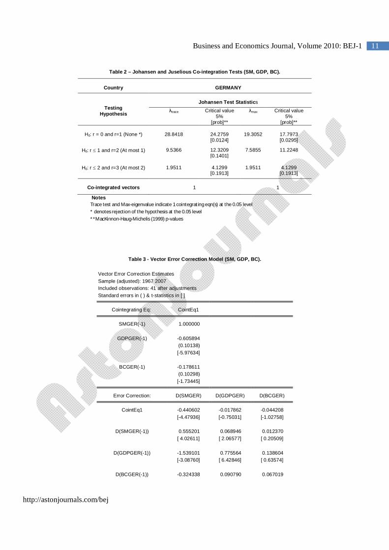
It is well known that Johansen‘s co-integration tests are very sensitive to the choice of lag length. Firstly, a VAR model is fitted to the time-series data in order to find an appropriate lag structure. The Schwarz Criterion (SC) and the likelihood ratio (LR) test are used to select the number of lags required in the co-integration test. The Schwarz Criterion (SC) and the likelihood ratio (LR) test suggested that the value p=1 is the appropriate specification for the order of VAR model for Germany. Table 2 presents the results from the Johansen and Juselious [26, 29] co-integration test.

2.4. Vector error correction model: Since the variables included in the VAR model are found to be co-integrated, the next step is to specify and estimate a Vector Error Correction Model (VECM) including the error correction term to investigate dynamic behaviour of the model. Once the equilibrium conditions are imposed, the VEC model describes how the examined model is adjusting in each period towards its long-run equilibrium state.

Since the variables are co-integrated, so, in the short run, deviations from this long-run equilibrium will feed back on the changes in the dependent variables in order to force their movements towards the long-run equilibrium state. Hence, the co-integrated vectors from which the error correction terms are derived are each indicating an independent direction where a stable meaningful long-run equilibrium state exists.

The VEC specification forces the long-run behaviour of the endogenous variables to converge to their co-integrated relationships, which accommodates short-run dynamics. The dynamic specification of the model allows the deletion of the insignificant variables, while the error correction term is retained. The size of the error correction term indicates the speed of adjustment of any disequilibrium towards a long-run equilibrium state [28]. The error-correction model with the computed t-values of the regression coefficients in parentheses is reported in Table 3.

The final form of the Error-Correction Model (ECM) was selected according to the approach suggested by Hendry [33]. The general form of the vector error correction model (VECM) is the following one:

titit

n

i

n

i

n

iititt ECZ

3210 (2.4)

where Δ is the first difference operator, ECt-1 is the error correction term lagged one period, λ is the short-run coefficient of the error correction term (-1<λ<0), εt is the white noise term.

2.5. Granger causality tests: Granger causality is used for testing the long-run relationship between stock market development and economic growth. The Granger procedure is selected because it consists the more powerful and simpler way of testing causal relationship [34]. The following bivariate model is estimated:


6 Research Article

t

k

jjtjjt

k

jjt uXbYaaY

11

1110 (2.5a)

t

k

jjtjjt

k

jjt uYbXaaX

12

1220 (2.5b)

where Yt is the dependent and Xt is the explanatory variable and ut is a zero mean white noise error term in Eq (2.5a), while Xt is the dependent and Yt is the explanatory variable in Eq (2.5b).

In order to test the above hypotheses the usual Wald F-statistic test is utilised, which has the following form

)12/(/)(

qTRSSqRSSRSS

FU

UR

where

RSSU= is the sum of squared residuals from the complete (unrestricted) equation RSSR= the sum of squared residuals from the equation under the assumption that a set of variables is redundant, when

the restrictions are imposed, (restricted equation) T = the sample size and q = is the lag length.

The hypotheses in this test are the following:

H0: X does not Granger cause Y, i.e. {α11, α12,…...α1k}=0, if Fc < critical value of F.

Ha: X does Granger cause Y, i.e. {α11, α12,…….α1k}≠0, if Fc > critical value of F. (2.6a)

and

H0: Y does not Granger cause X, i.e. {β21, β22,...β2k}=0, if Fc < critical value of F.

Ha: Y does Granger cause X, i.e. {β21, β22,….β2k}≠0, if Fc > critical value of F. (2.6b)

[35].

The results related to the existence of Granger causal relationships among economic growth, stock market development, and bank lending are presented in Table 4.

3. Empirical results

The observed t-statistics in the table 1 fail to reject the null hypothesis of the presence of a unit root for all variables in their levels confirming that they are non-stationary at 1% and 5% levels of significance. The combined results (ADF, PP, KPSS) from all tests show that the null hypothesis of the presence of a unit root is rejected for all variables when they are transformed into their first differences (Table 1). Therefore, all series that are used are non-stationary in their levels, but stationary in their first differences (integrated of order one I(1). Therefore, following Dritsakis and Adamopoulos



[30] these variables can be co-integrated as well, if there are one or more linear combinations among the variables that are stationary.

The results that appear in Table 2 suggest that the number of statistically significant co-integration vectors for Germany is equal to 1. The process of estimating the rank r is related with the assessment of eigenvalues, which are the following

for Germany: 1

0.3755, 2

0.1689, and 3

0.0464. For Germany, critical values for the trace statistic defined by equation (2.3a) are 24.27 for Ηο: r = 0, 9.53 for Ηο: r1, and 1.95 for Ηο: r2 at the significance level 5% respectively as reported by Osterwald-Lenum [36], while critical values for the maximum eigenvalue test statistic defined by equation (2.3b) are 19.30 for Ηο: r = 0, 7.58 for Ηο: r 1, 1.95 for Ηο: r2 (Table 2).

It is obvious from the above co-integrated vector that economic growth and bank lending have a positive effect on stock market development in the long run. According to the signs of the vector co-integration components and based on economic theory, the above relationships can be used as an error correction mechanism in a VAR model for Germany respectively. The best VAR model in which economic growth is examined as a dependent one is selected by the three VAR models that can be estimated respectively.

The results of the estimated vector error correction model suggest that a short-run increase of stock market index per 1% induces an increase of economic growth per 0.06% in Germany and an increase of bank lending per 1% induces an increase of economic growth per 0.9% in Germany. The estimated coefficient of ECt-1 is statistically significant and has a negative sign, which confirms that there is no problem in the long-run equilibrium relation between the independent and dependent variables in 5% level of significance, but its relatively value (-0.017) for Germany shows a satisfactory rate of convergence to the equilibrium state per period (Table 3). In order to proceed to the Granger causality test the number of appropriate time lags was selected in accordance with the VAR model. According to the results of Table 4, it can be inferred that indicated that there is a unidirectional causality between stock market development and economic growth with direction from stock market development to economic growth.

4. Discussion

This model of financial system investigates the causal relationship among economic growth, stock market development and bank lending. Stock market development is determined by the trend of general stock market index. The significance of the empirical results is dependent on the variables under estimation. Most empirical studies examine the relationship between economic growth and financial market development using different estimation measures. The most representative estimation measures for financial market development are the general stock market index, stock market liquidity and bank credits to private sector. The general stock market index expresses the trend of stock market development in conjunction with the investment growth and the low interest rate. Theory provides conflicting aspects for the impact of stock market development on economic growth or vice-versa. Very few empirical studies have concentrated on examining the causal relationship between economic growth and stock market development and bank lending. The results of many empirical studies examining the relationship between stock market development and economic growth differ, relatively to the sample period, the examined countries, the measures of financial development, and the estimation method. The results of this paper are agreeable with the studies of Levine and Zervos; King and Levine [2, 9]. The direction of causal relationship between stock market development and economic growth is regarded as an important issue under consideration in future empirical studies. However, more interest should be focused on the comparative analysis of empirical results for the rest of European Union member-states.

5. Conclusion

This paper examines empirically the relationship between stock market development and economic growth for Germany, using annual data for the period 1965-2007. The empirical analysis suggested that the variables that


8 Research Article

determine economic growth present a unit root. Once a co-integrated relationship among relevant economic variables is established, the next issue is how these variables adjust in response to a random shock. This is an issue of the short-run disequilibrium dynamics. The short run dynamics of the model is studied by analysing how each variable in a co-integrated system responds or corrects itself to the residual or error from the cointegrating vector. This justifies the use of the term error correction mechanism. The error correction (EC) term, picks up the speed of adjustment of each variable in response to a deviation from the steady state equilibrium. The VEC specification forces the long-run behaviour of the endogenous variables to converge to their co-integrating relationships, which accommodates the short-run dynamics. The dynamic specification of the model suggests deletion of the insignificant variables while the error correction term is retained. The results of Granger causality tests indicated that there is a unidirectional causality between stock market development and economic growth with direction from stock market development to economic growth.

Competing Interests

The author declares that he has no competing interests.

References

[1] Demirguc-Kunt A, Levine R, 1996. Stock markets corporate finance and economic growth. World Bank Economic Review, 10(2): 223-240.

[2] Levine R, Zervos S, 1998. Stock markets, banks and economic growth. American Economic Review, 88(3): 537-558.

[3] Pagano M, 1993. Financial markets and growth: An overview. European Economic Review, 37: 613-622.

[4] Obstfeld M, 1994. Risk-Taking, Global Diversification, and Growth. American Economic Review, 84: 1310-1329.

[5] Kahn M, Sendahji A, 2000. Financial development and economic growth: An overview, IMF Working Paper, WP/00/209, International Monetary Fund.

[6] Caporale G, Howells P, Soliman A, 2005. Endogenous Growth Models and Stock Market Development: Evidence from Four Countries. Review of Development Economics, 9(2): 166–176.

[7] Fama E, 1990. Stock returns, expected returns, and real activity. Journal of Finance, 45: 1089-1108.

[8] Schwert W, 1990. Stock returns and real activity: a century of evidence. Journal of Finance, 45: 1237-1257.

[9] King R, Levine R, 1993a. Finance and Growth: Schumpeter Might be Right. Quarterly Journal of Economics, 108(3): 717-737.

[10] Vazakidis A, Adamopoulos A, 2009b. Financial development and economic growth: An empirical analysis for Greece. American Journal of Applied Sciences, 6(7): 1408-1415.

[11] Vazakidis A, Adamopoulos A, 2009d. Stock market development and economic growth: an empirical analysis for Greece. Published to the Proceedings of International Conference of ICABE 2009, [http://www.icabe.gr] accessed November 1, 2009.



[12] Katsouli E, 2003. Book review: Money, Finance and Capitalist Development, In Philip Arestis and Malcolme Sawyer, (March 2003), Economic Issues.

[13] Nieuwerburgh S, Buelens F, Cuyvers L, 2006. Stock market and economic growth in Belgium. Explorations in Economic History, 43(1): 13-38.

[14] Shan J, 2005. Does financial development lead economic growth? - A vector auto-regression appraisal. Applied Economics, 37: 1353-1367.

[15] Vazakidis A, 2006. Testing simple versus Dimson market models: The case of Athens Stock Exchange. International Research Journal of Finance and Economics, 2: 26-34.

[16] Vazakidis A, Adamopoulos A, 2009a. Credit market development and economic growth. American Journal of Economics and Business Administration, 1(1): 34-40.

[17] Vazakidis A, Adamopoulos A, 2009c. Stock market development and economic growth. American Journal of Applied Sciences, 6(11): 1933-1941.

[18] Adamopoulos A, 2010. Financial development and economic growth: A comparative study between 15 European Union member-states. International Research Journal of Finance and Economics, 35: 143-149.

[19] International Monetary Fund, 2007. International Financial Statistics Yearbook, 2007, Washington DC: Various Years.

[20] Dickey D, Fuller W, 1979. Distributions of the Estimators for Autoregressive Time-series with a Unit Root. Journal of American Statistical Association, 74: 427- 431.

[21] Akaike H, 1973. Information Theory and an Extension of the Maximum Likelihood Principle, In: Petrov, B. and Csaki, F. (eds) 2nd International Symposium on Information Theory. Budapest: Akademiai Kiado.

[22] Schwarz R, 1978. Estimating the Dimension of a Model. Annals of Statistics, 6: 461-4.

[23] Phillips P, Perron P, 1988. Testing for a unit root in time-series regression. Biometrika, 75: 335-346.

[24] Choi I, 1992. Effects of Data Aggregation on the Power of the Tests for a Unit Root. Economics Letters, 40: 397-401.

[25] Kwiatkowski D, Phillips P, Schmidt P, Shin Y, 1992. Testing the null hypothesis of stationarity against the alternative of a unit root. Journal of Econometrics, 54: 159-178.

[26] Johansen S, Juselious K, 1990. Maximum Likelihood Estimation and Inference on Co-integration with Applications to the Demand for the Money. Oxford Bulletin of Economics and Statistics, 52: 169 - 210.

[27] Johansen S, Juselious K, 1992. Testing Structural Hypotheses in a Multivariate Co-integration Analysis at the Purchasing Power Parity and the Uncovered Interest Parity for the UK. Journal of Econometrics, 53: 211- 244.

[28] Engle R, Granger C, 1987. Co-integration and error correction: Representation, estimation and testing. Econometrica, 55: 251-276.

[29] Johansen S, 1988. Statistical Analysis of Co-integration Vectors. Journal of Economic Dynamics and Control, 12: 231-254.


10 Research Article

[30] Dritsakis N and Adamopoulos A, 2004. Financial development and economic growth in Greece An empirical investigation with Granger causality analysis. International Economic Journal, 18: 547-559.

[31] Phillips P, 1987. Time-series Regression with Unit Roots. Econometrica, 2: 277-301.

[32] Newey W, West K, 1987. A Simple, Positive Semi-Definite, Heteroskedasticity and Autocorrelation Consistent Covariance Matrix. Econometrica, 55: 703-708.

[33] Maddala G, 1992. Introduction to Econometrics, Prentice Hall, New Jersey.

[34] Granger C, 1986. Developments in the study of co-integrated economic variables. Oxford Bulletin of Economics and Statistics, 48: 213-228.

[35] Katos A, 2004. Econometrics: Theory and practice, Thessaloniki: Zygos.

[36] Osterwald-Lenum M, 1992. A Note with Quantiles of the Asymptotic Distribution of the Maximum Likelihood Co-integration Rank Test Statistics. Oxford Bulletin of Economics and Statistics, 54: 461-472.

[37] Chang, T, 2002. An econometric test of Wagner's law for six countries based on cointegration and error-correction modelling techniques. Applied Economics, 34(9): 1157–1169.

[38] Chang T, Caudill S, 2005. Financial development and economic growth: the case of Taiwan. Applied Economics, 37(12): 1329–1335.

[39] Seddighi H, Lawler K, Katos A, 2000. Econometrics: A Practical Approach. London: Routledge.

Table 1 -Tests of Unit Roots Hypothesis. Augmented Dickey-Fuller Phillips-Perron KPSS

ADF_test

stat

Lag eq_f

PP_ test stat

LM test stat

tn tc tt hc ht GERMANY SM -2.91

[0.16] p=1

(2.2c) 1.09

(for k=3) -0.02

(for k=3) -2.30

(for k=2) 0.75

(for k=5) 0.17*** (for k=3)

BC -0.97 [0.93]

p=1 (2.2c)

1.67 (k=4)

-1.76 (k=4)

-1.36 (k=4)

0.77 (l=5)

0.29 (l=0)

GDP -2.46 [0.34]

p=1 (2.2c)

3.69 (for k=4)

0.74 (for k=4)

-2.32 (for k=4)

0.80 (for k=5)

0.14*** (for k=5)

ΔSM -3.78 [0.00]

p=0 (2.2a)

-3.79 (for k=3)

-3.85 (for k=4)

-3.73 (for k=5)

0.15 (for k=2)

0.03 (for k=3)

ΔBC -4.60 [0.00]

p=1 (2.2c)

-5.61 (k=0)

-6.09 (k=4)

-6.39 (k=4)

0.23 (l=4)

0.07 (l=4)

ΔGDP -3.04 [0.03]

p=0 (2.2b)

-1.16*,**,***(for k=3)

-3.05*** (for k=1)

-3.15*,**,****(for k=1)

0.24 (for k=4)

0.12* (for k=4)

Notes: The calculated statistics are those reported in Dickey-Fuller (1981).The critical values for SM and GDP at 1%, 5% and 10% are -4.19, -3.62, -3.19, for BC, ΔBC at 1%, 5% and 10% are -4.19, -3.52, -3.19, for ΔSM at 1%, 5% and 10% are -2.62, -1.94, -1.61, for ΔGDP at 1%, 5% and 10% -3.60*, - 2.93, -2.60 respectively. The lag-length (p) structure of aΙ of the dependent variable xt is determined using the recursive procedure in the light of a Langrange multiplier (LM) autocorrelation test (for orders up to two), which is asymptotically distributed as chi-squared distribution and the value t- statistic of the coefficient associated with the last lag in the estimated autoregression. The critical values for the Phillips-Perron unit root tests are obtained from Dickey-Fuller. tn, tc and tt are the PP statistics for testing the null hypothesis the series are not I(0) when the residuals are computed from a regression equation without an intercept and time trend, with only an intercept, and with both intercept and time trend, respectively. The critical values at 1%, 5% and 10% are -2.62, -1.94, -1.61, for tn, -3.60, -2.93, -2.60 for tt, and for -4.19, -3.52, -3.19 for tτ respectively. k= bandwidth length: Newey-West using Bartlett kernel. hc and ht are the KPSS statistics for testing the null hypothesis that the series are I(0) when the residuals are computed from a regression equation with only an intercept and intercept and time trend, respectively. The critical values at 1%, 5% and 10% are 0.73, 0.46 and 0.34 for hc and 0.21, 0.14 and 0.11 for ht respectively [25]. Since the value of the test will depend upon the choice of the ‘lag truncation parameter’, l. l= bandwidth length: Newey-West using Bartlett kernel. ***, **, * indicate that those values are not consistent with relative hypotheses at the 1%, 5% and 10% levels of significance relatively.



Table 2 – Johansen and Juselious Co-integration Tests (SM, GDP, BC).

Country

GERMANY

Testing Hypothesis

Johansen Test Statistics

λtrace Critical value 5%

[prob]**

λmax Critical value 5%

[prob]**

H0: r = 0 and r=1 (None *)

28.8418

24.2759 [0.0124]

19.3052

17.7973 [0.0295]

H0: r 1 and r=2 (At most 1) 9.5366 12.3209 [0.1401]

7.5855 11.2248

H0: r 2 and r=3 (At most 2)

1.9511

4.1299

[0.1913]

1.9511

4.1299

[0.1913]

Co-integrated vectors

1

1

Notes Trace test and Max-eigenvalue indicate 1 cointegrating eqn(s) at the 0.05 level * denotes rejection of the hypothesis at the 0.05 level **MacKinnon-Haug-Michelis (1999) p-values

Table 3 - Vector Error Correction Model (SM, GDP, BC).

Vector Error Correction Estimates Sample (adjusted): 1967 2007 Included observations: 41 after adjustments Standard errors in ( ) & t-statistics in [ ]

Cointegrating Eq: CointEq1 SMGER(-1) 1.000000

GDPGER(-1) -0.605894 (0.10138) [-5.97634]

BCGER(-1) -0.178611 (0.10298) [-1.73445] Error Correction: D(SMGER) D(GDPGER) D(BCGER) CointEq1 -0.440602 -0.017862 -0.044208 [-4.47936] [-0.75031] [-1.02758]

D(SMGER(-1)) 0.555201 0.068946 0.012370 [ 4.02611] [ 2.06577] [ 0.20509]

D(GDPGER(-1)) -1.539101 0.775564 0.138604 [-3.08760] [ 6.42846] [ 0.63574]

D(BCGER(-1)) -0.324338 0.090790 0.067019


12 Research Article

[-0.84622] [ 0.97872] [ 0.39979]

R2 0.421772 0.390310 0.016623 Adj. R2 0.374888 0.340875 -0.063110 Sum sq. resids 0.174382 0.010215 0.033358 S.E. equation 0.068651 0.016616 0.030026 F-statistic 8.996185 7.895510 0.208482 Akaike AIC -2.427081 -5.264490 -4.081026 Schwarz SC -2.259903 -5.097312 -3.913849

VEC Residual Serial Correlation LM Tests 3.6585 [0.9324]

VEC Residual Normality Tests Jarque-Bera 1.1168 [0.5721] [ ]= I denote the t-statistics Δ: Denotes the first differences of the variables. Adj. R2 = Coefficient of multiple determinations adjusted for the degrees of freedom (d.f),

Table 4 – Pairwise Granger Causality Tests.

Sample: 1965 2007 Lags: 3

Null Hypothesis:

Obs Wald F-Statistic Probability

GDP does not Granger Cause SM

42

5.6885

0.0220

SM does not Granger Cause GDP

0.3489

0.5581

BC does not Granger Cause SM

42

2.1726

0.1485

SM does not Granger Cause BC

0.3489

0.5648

BC does not Granger Cause GDP

42

0.1176

0.7335

GDP does not Granger Cause BC

1.5324

0.2231

stock market and economic growth: an empirical...

Documents