Trade Openness and Gender in Uruguay: a CGE Analysis1

October 2007

María Inés Terra, Marisa Bucheli and Carmen Estrades2

dECON, UdelaR, Uruguay

1 This work was carried out with financial and scientific support from Poverty and Economic Policy (PEP) Research Network, which is financed by the Australian Agency for International Development (AusAID) and the Government of Canada through the International Development Research Centre (IDRC) and the Canadian International Development Agency (CIDA). The authors acknowledge the collaboration of Rodrigo Ceni who participated in different phases of the study. We are very thankful for the comments received from Marzia Fontana, Wilfredo Maldonado, Masakazu Watanuki, André Lemelin and Renato Flores, Bernard Décaluwé, Ismaël Fofana, Veronique Robichaud, John Cockburn and Silvia Laens. All remaining errors and omissions are our own responsibility. 2 Departamento de Economía, Facultad de Ciencias Sociales, Universidad de la República, Uruguay. Mailing address: Constituyente 1502, 6to piso, Montevideo, Uruguay. E-mail addresses: iterra@decon.edu.uy; marisa@decon.edu.uy, carmen@decon.edu.uy.

2

Abstract

In this paper we analyze the gender differentiated impacts of trade openness in Uruguay

using a gender aware CGE model with endogenous labor supply and a home production function.

We simulate complete trade liberalization and an increase in tariffs to the level of 1994. Trade

liberalization increases female employment and wages, reducing the gender wage gap. These

findings are consistent with Çagatay (2001) and Fofana et al (2003). The effect of trade openness on

time distribution of workers is different by skills. Skilled workers, mainly women, reduce time

spent in leisure and domestic work increasing labor supply. In contrast, unskilled workers increase

leisure time, especially men. Trade openness leads to a more equitable distribution of time spent in

domestic work. When there is a more imperfect substitution among genders in the home production

function, women reduce more leisure time. The increase in tariff to the level of 1994 has the

opposite results.

Keywords: trade openness, gender, general equilibrium model, home production, leisure, wage curve

JEL classification: D68, D13, J16, J22, F16

3

1. Introduction

Uruguay is a small Latin American country that has strong comparative advantages

in agriculture. In the 1990s unilateral trade liberalization and integration with MERCOSUR

partners led to a significant reduction of protection to the domestic market. As a

consequence, there was a change in relative prices and a reallocation of resources from

manufacture to service sector. Women participation in labor market increased, although

there is evidence that in 2003 women assign less time assigned to labor market than men,

while the opposite happens with time assigned to domestic work. Additionally, some

studies conclude that gender discrimination in the labor market persists.

In principle, a country may benefit from trade openness because it causes an

increase of trade and productive specialization. Productive efficiency increases due to a

better resource allocation and at the same time, welfare rises through an improvement of

consumption possibilities. Furthermore, when imperfect competition exists, openness may

report additional benefits through the access to a larger variety in consumption of

differentiated goods, the use of economies of scale and the fall in prices induced by the

decline of monopoly rents. However, international trade leads to changes in relative prices

of goods, in relative demands of productive factors and as a consequence, in their relative

remuneration. This means that we may expect changes in income distribution. In particular,

trade openness may have gender-differentiated effects.

There are three different mechanisms through which trade openness affects labor

market by gender. First, the gender distribution of the impact in terms of employment will

depend on the sectoral intensity in the use of male and female labor. If trade openness

benefits sectors intensive in male (female) labor, men (women) employment will improve.

The second mechanism stems from this effect. Indeed, the changes in the relative demand

by gender affect the earnings gender gap. Therefore, we may expect that a female intensive

sectors growth would decrease the gender gap. Anyway, labor discrimination will

contribute to widen or reduce the effect on the gender gap. A third source comes from the

change in labor supply induced by modifications in employment opportunities and wages.

Therefore, it is important to evaluate the intra-household reallocation of resources.

4

Other aspects, such as public provision of social services, might also be affected,

but empirical studies rarely focus on them. Most of the empirical work study whether trade

policies affect women’s employment relative to men and the earnings gender gap. In

contrast, evidence about the effects on the time allocation among household members is

less frequent. Some gender-aware CGE models allow to measure these three sources of

impact via incorporating a home production function and three activities to spend time in

(market work, domestic work and leisure) as proposed by Fontana and Wood (2000).

Following this strategy, different results were obtained for Nepal (Fofana, Cockburn

and Décaluwé, 2003), South Africa (Fofana et al, 2005), Pakistan (Siddiqui, 2007),

Bangladesh and Zambia (Fontana, 2003), when simulating an abolition of tariffs. In the five

countries, time of women in labor market rises but the gender wage gap decreases only in

three of them. The effect on domestic work and leisure is neither conclusive. For example,

in Bangladesh, the increase in the opportunity cost of working for women –due to the

decline of the gender wage gap- leads to some substitution of male and female in home

production. In Nepal, in spite of a decline of the gender wage gap, women do not benefit

with a reduction of time spent in domestic work. In fact, female entrance to the labor

market is accomplished with a decrease of leisure time as men’s leisure time rises. Thus,

trade openness seems to have more equitable effects in Bangladesh.

The aim of this paper is to analyze the gender-differentiated effects of complete

trade openness in Uruguay, following the methodological strategy pursued by the above

mentioned literature. Specifically, we study the effects on wages, employment, allocation

of time between labor market and domestic work, and income distribution, using a gender-

aware CGE model.

The paper is organized as follows. First, we present an introduction to the

Uruguayan economy in general and to labor market in particular. Secondly, we present the

model and the data we use. Then, we analyze the results of three different trade policy

scenarios. Finally, we draw some conclusions.

5

2. The Uruguayan Economy

2.1. Trade openness

Uruguay is a small country whose population - about 3.4 million in 2005- live

mostly in urban areas (92 percent). Traditionally, production and exports have relied on

agriculture, husbandry and meat processing. As many Latin American countries, in the

1990s Uruguay underwent through an important process of trade openness and

liberalization of capital markets. Although the liberalization process had started in the

1970s, it deepened in the 1990s. From 1990 to 1995 there was a significant tariff reduction

as a result of unilateral trade liberalization and trade integration within MERCOSUR

(Common Market of the South). The two processes can be easily identified in figure 1,

which presents the average tariff protection within MERCOSUR and the average tariff

applied to the rest of the world. As we can see, the average protection reduced significantly

until 1995. Although in the last ten years the average tariff applied to imports from the rest

of the world has not been much modified, the intra- MERCOSUR tariff is practically zero.

Figure 1. Uruguay: Average tariff protection, 1991- 2004

Source: Secretaría del MERCOSUR

The process of trade openness affected labor market in many ways. First of all, there

was an important restructure of employment. Manufacturing lost importance both in GDP

and employment: while in 1990 the sector employed 23.3 percent of workers, in 1999 this

0

5

10

15

20

25

1991 1992 1993 1994 1995 1996 1997 1998 1999 2000 2001 2002 2003 2004

Ad

valo

rem

tari

ff

Intra-MERCOSUR Rest of the world

6

percentage fell to 15.9 percent. On the other hand, the share of services and traditional

export activities in employment gained importance.

Second, the dispersion of labor earnings increased. One of its most important

sources was the rise of the rewards to education. As additionally unemployment and

informality increased affecting mainly unskilled workers, we may interpret that the relative

demand for skilled labor has increased. Casacuberta and Vaillant (2004) argue that this rise

was due to the adoption of new technologies -complementary to skilled labor- that was

induced by trade liberalization.

2.2. Gender in the Uruguayan economy

Since the middle of the 1980s, women’s participation in the labor market has had an

increasing trend meanwhile men’s one have presented a little decline. Table 1 shows this

evolution for the group of 18 to 54 years old: female participation rate rose from 62 percent

in 1986-1990 to 72 percent in 2001-2004 and male rate decreased from 94 percent to 92

percent in the same period.

Table 1. Labor characteristics of the group of 18 to 54 years old

1986-1990 1991-2000 2001-2004 Women Participation rate 61.7 68.4 71.9 Unemployment rate 12,3 13,5 19,9 Employment rate 54.1 59.1 57.2 Men Participation rate 94.1 93.3 92.1 Unemployment rate 6,2 7,5 12,0 Employment rate 88.2 86.3 80.9 Wage gap (log difference) * All 0.146 0.098 0.009 Private sector 0.273 0.160 0.074 Public sector -0.170 -0.086 -0.178 * Only employees (self-employment excluded)

Source: Continuous Household Survey

There are several empirical works focusing on female participation in labor market

in Uruguay that conclude that it increases with the education level and decreases with

household’s income and age. Besides, it is lower for married women and for women with

little children, although the likelihood of participation increases when children grow (Diez

de Medina, 1992; De Soria, Rivas and Taboada, 2001). In a study restricted to couples,

7

Bucheli (2002) found that female participation is more likely for women who live with

inactive elderly people or whose husband is unemployed.

Obviously, time spent in labor market also depends on the likelihood of being

employed. As shown in table 1, female unemployment rate has been persistently higher

than male unemployment in spite of the increase of women labor market participation.

Unemployment is particularly high for non-skilled women who also suffer a relative high

duration of unemployment.

Table 1 also reports the raw gender wage gap measured as the difference of the male

and female mean log hourly wage. The gap was positive in 1986-90 and since then, has had

a decreasing trend. In recent years, its value has been close to zero. In spite of these figures,

several studies point out the presence of gender discrimination in the labor market.

Indeed, some Uruguay literature follows the spirit of Oaxaca’s proposal to measure

gender discrimination. According to this proposal, the raw gender gap may be decomposed

in two terms. One of them stems from the gender difference in endowments and the other

one, from the gender difference in endowments’ rewards. The latter is a measure of gender

discrimination.

The broad conclusion of Uruguayan studies is that the raw gap cannot be totally

explained by endowments. Therefore, we may interpret that there is labor market

discrimination. According to Bucheli and Sanromán (2005) the discrimination measure

increases throughout the wage distribution. Furthermore, there is a sharp acceleration in the

upper distribution, which they interpret as evidence of a glass ceiling.

Rivas and Rossi (2000) find that the decline of the raw gap in the 1990s in the

private sector was mainly due to an improvement of women’s human capital and, in a less

extent, to a change in endowments’ rewards. They conclude that at the end of the decade,

discrimination took account for more than 100% of the raw gender gap in the private labor

market. This overall picture does not fit for public wage earners. Rivas and Rossi (2002)

compare private and public wage earners in the nineties and conclude that gender

discrimination increased for the former but decreased for the latter. Furthermore, Amarante

(2001) finds that at the end of the 1990s, there was not evidence of discrimination in the

public sector.

8

When employed, women and men present different distribution among occupations

and industries. In broad terms, we may say that women tend to concentrate in fewer jobs

than men. According to Amarante and Espino (2001), this gender distribution among

occupations reflects a segregation phenomenon and in the 1990s, it has had an increasing

trend in the private wage earners labor market. In contrast, segregation has been lower and

stable in the public sector.

Time spent in non-remunerated work has been less studied than time in labor

market. There is a single survey in Uruguay that collects information about use of time,

carried out in 2003. Its main figures are reported in Aguirre and Batthyány (2005). The

survey for time use does not collect information about education or income of the

household. Thus, we match the data provided by this survey and the Household Survey in

order to estimate the amount of hours assigned to domestic and labor market work by

gender and educational level. The methodological aspects about this match are presented in

the Annex 1.

In table 2 we show the estimation of the time distribution for women and men of 14

to 65 years old. We suppose that people –regardless of their sex or education level- assign

10 daily hours to personal care, that is, a minimum time needed for sleeping, feeding,

hygiene and health care. According to these estimations, women spend 16% of their time in

domestic work and 11% in labor market work. The distribution is quite different for men:

the figures are 6% and 20%, respectively. In contrast, the gender difference in time

assigned to leisure is not so important.

We also report time distribution according to the worker’s level of education.

Regardless the education level, women assign more time to domestic work and men spent

more time at market work. Skilled women assign more time to market work than unskilled

women, but instead of reducing domestic work time, they reduce leisure time.

9

Table 2. Time assignment of population between 14 and 65 years old by gender.

In percentages All Less than 12 years of

schooling 12 years of schooling or

more Men Women All Men Women All Men Women All

Market work 20.2 11.1 15.4 19.2 9.3 14.1 23.5 15.3 18.7 Domestic work 5.6 16.2 11.2 5.5 16.7 11.2 5.9 15.1 11.3 Leisure 32.5 31.0 31.7 33.7 32.3 33.0 28.9 27.9 28.3 Personal care 41.7 41.7 41.7 41.7 41.7 41.7 41.7 41.7 41.7 Total 100.0 100.0 100.0 100.0 100.0 100.0 100.0 100.0 100.0

Source: Own estimations based on Survey on the Use of Time and CHS

3. Model and Calibration

The effects of trade liberalization on macro and microeconomic variables are

estimated using a CGE model. In this section we present an overview of the model and its

calibration. The core model is based on Laens and Terra (1999, 2000) and Terra et al

(2006). Its structure is quite conventional in terms of the analysis of trade-related issues but

we work with alternative specifications regarding the labor market in order to take into

account gender issues. Specifically, we use three different versions of the model: first, we

disaggregate male and female labor demand (model 1), second, we consider male and

female labor supply as endogenous (model 2) and third, we incorporate domestic work in

the model (model 3).

3.1. Model

The general structure of the CGE model is quite conventional. Uruguay is assumed

to be a quasi-small economy (following Harris, 1984) that has three trading partners:

Argentina, Brazil and the rest of the world. The Uruguayan economy is explicitly modeled,

while import demand from the trading partners is assumed to be perfectly elastic and export

demand presents a downward slope that is a negative function of export prices in Uruguay.

We assume perfect competition in all sectors, and goods are differentiated by geographic

origin (Armington, 1969). There are ten representative households according to level of

income. Government collects taxes, pays transfers to household and buys goods.

Government savings is obtained as a residual. Complete core model and equations are

presented in Annex 2.

10

The model presents two distinctive features. In the first place, the labor market

module follows a wage curve behavior specification, introducing unemployment, which

affects only unskilled workers, both men and women. There are different interpretations

about the existence of a negative relationship among wages and unemployment

(Blanchflower and Oswald, 1994). One of them is the existence of efficiency wages, paid

by firms in order to promote effort or reduce the quitting rate among workers. When

unemployment rises the wage needed to promote workers’ efficiency declines.

Secondly, we extend the model in order to allow the introduction of gender

differences. The previous CGE model versions did not disaggregate labor by gender and

assumed labor participation as exogenous. We relax these assumptions by steps as in

Fofana et al (2003, 2005).

First, in Model 1 we disaggregate female and men labor demand. This means to

relax the assumption of perfect substitution between men and women in production.

Following Fontana (2001) we assume identical substitution elasticity for all sectors. Gender

segmentation in the labor market allows assessing a differentiated-gender impact on wages

and employment due to the changes in sectoral structure.

There are five factors of production: skilled female labor, skilled male labor,

unskilled female labor, unskilled male labor and capital.

As the model has four types of labor, the average wage is a combination of skilled

female, skilled male, unskilled female and unskilled male wage. Following Laens and Terra

(1999), we assume a nested production function. At the top level, a Cobb Douglas function

combines intermediate inputs and value added. At the second level, value added is

composed by capital and labor. At the third level, labor is a composed factor of skilled and

unskilled labor. Finally, a new equation that combines labor by sex in order to get a

composite labor by education is included in the model. Figure 2 presents more clearly the

nested production function for this model.

11

Figure 2. Production function of the firm

Labor by gender is combined following a CES function: )1/(1

.))1.(( 1,,,,,

ig

ii gi

gisg

gisgis gtfacwlws

θ

θθ ξ

−

⎥⎦

⎤⎢⎣

⎡+= −∑

In which isws , is the wage for composite labor by skills, wlg, s, i are the wages for

each labor type respectively, tfac is the labor tax rate, ξg is the distribution parameter, and

θgi is the elasticity of substitution between men and women. Subindex s refers to a subset

that includes labor categories by skills (skilled and unskilled), subindex g refers to labor

categories by gender (male and female) and subindex i refers to sectors.

Then, to get a factor of aggregated labor (l), labor by skills is combined in the firm’s

production function following the CES function: )1/(1

..)( 1,

i

iii

sisli wsw

θ

θθ ξ−

⎥⎦

⎤⎢⎣

⎡= −∑

in which liw is the wage for aggregated labor, ξi is the distribution parameter and θi

is the elasticity of substitution between labor by skill.

12

In a second step, we relax the assumption of exogenous labor force and we

introduce non-labor market time, which is composed by both leisure and domestic work.

Thus, Model 2 introduces the idea that men and women are not perfect substitutes in non-

labor market. As we need to subtract from the available time the minimum subsistence

volumes of non-market work required, we follow Fontana and Wood (2000) who propose

to fix this minimum volume in 10 hours per day.

Domestic work at home and leisure are introduced in the utility function of the

households, but we assume them to be perfect substitutes. Each household maximizes its

utility subject to a budget constraint, which includes market income earned by the

household plus non-labor income.

Utility function is a Cobb – Douglas function that combines consumption of leisure

by type of labor (L) and of market goods (C) for each type of household:

∏=i

ifffemfmalU CLLifffemfmal

f

μμμ.,,

,,

From the optimization of the utility function, we can derive labor supply equations

(lslab,f) and final goods demand of households (cif):

lablab

flab

fffflabflabflab w

msavtdyhsls

∑−

−−−=

).1()1)(1(.

max,

,,, μ

μ

Where max hslab,f is the maximum hours available for leisure and work, and is

considered a fixed parameter in the model, )1)(1( fff msavtdy −− represents households’

available income and wlab is the wage for each type of labor.

Finally, Model 3 considers that households use part of their time to produce home

goods, which are consumed by themselves. Thus, we distinguish between leisure and

domestic work. Additionally, the model requires fixing an elasticity of substitution between

male and female labor in home production. Following previous works (Fontana and Wood,

2000), we fix it at a lower level than the elasticity of substitution between men and women

in labor market, in order to reproduce the rigidity of labor at the household level.

∑−−−

=

labiflab

fffifif pf

msavtdyc

).1()1)(1(.

,μμ

13

In this case, households’ utility is a function of the consumption of market produced

goods, home goods (CZ) and leisure.

∏=i

iffffemfmalU CCZLLiffffemfmal z

f

μμμμ.,,

,,

Labor supply is now:

Where lzlab,f is the time used by different labor categories to domestic work.

The final goods demand of households also changes:

And a new equation that determines demand of domestic goods is introduced:

Home goods are produced and consumed by the same family.

Minimizing the costs of production of domestic goods subject to the production

function, we obtain the price of domestic goods (pzf) and the demand of work for

production of domestic goods (lzlab,f):

Where flabh ,α is the share parameter in the CES production function, AHf is the

scale parameter and ρf = (1- σzf)/ σzf

lablab

fflab

fffflabflabflabflab wz

msavtdylzhsls

∑ −−−−

−−=).1(

)1)(1(.max

,

,,,, μμ

μ

∑ −−−−

=

labifflab

fffifif pfz

msavtdyc

).1()1)(1(.

, μμμ

∑ −−−−

=

labffflab

fffff pzz

msavtdyzcz

).1()1)(1(.

, μμμ

f

lablab

flab

f AH

wlhpz

ff

fff

ρρρρρα

/)1(1/1/1

, .+

++

⎥⎦

⎤⎢⎣

⎡

=∑

fflab

flabfflab QZAH

wlhpz

lzff

f

..)1/(

1/1,

,

+−+

⎟⎟⎠

⎞⎜⎜⎝

⎛=

ρρρα

14

σzf being the elasticity of substitution between different labor categories in the

domestic good production function.

Finally, the equilibrium condition in the domestic good market is:

QZf = czf

In Annex 2 we present the calibration of parameters of the three versions of the model.

The model is run using software GAMS (General Algebraic Modeling System).

3.2. Calibration

We use data for year 2000 to calibrate the model, in the form of a Social Accounting

Matrix (SAM). Changes to the original SAM are described in detail in Terra et al (2006).

Basically, it has 23 sectors of production, one being an informal sector that only produces

for domestic market and the other one a public sector. Then, it has three factors of

production -skilled labor, unskilled labor and capital-, two national institutions –

households, presented in ten representative household according to level of income, and

government- and three trading partners –Argentina, Brazil and the rest of the world.

For the purposes of this paper, we modified the core SAM in order to adapt it to the

three specifications of the model, introducing the gender dimensions by steps.

As model 1 considers four types of labor, we distinguished them in the SAM, using

data from the Continuous Household Survey for year 2001. The factorial use of the sector is

now the following:

15

Table 3. Labor intensity by sector

Source: SAM

There are several male-intensive activities, such as agriculture, husbandry and other

primary activities, while health, export activities and other services employ a higher

percentage of women. In fact, female labor is concentrated in few sectors, as table 4 shows.

The activity “other services”, which includes private education, services to firms and

domestic service, concentrates almost 50 percent of total female labor. This figure is even

higher when we consider only skilled female labor, while unskilled women are employed in

more activities, such as informal activities, trade and transport (basically retail) and health.

Sector of activity (SAM)

Skilled female labor

Skilled male labor

Unskilled female labor

Unskilled male labor Total

Agriculture 3.0 27.6 8.0 61.5 100.0Husbandry 0.0 0.0 11.5 88.5 100.0Forestry 13.6 33.7 1.6 51.1 100.0Other primary 0.5 2.7 3.9 92.9 100.0Meat processing 4.3 10.4 21.3 64.0 100.0Dairy products 4.3 10.4 21.3 64.0 100.0Rice 4.3 10.4 21.3 64.0 100.0Tanning 2.9 15.6 17.7 63.8 100.0Wood and paper 0.6 6.8 12.0 80.5 100.0Chemicals 11.8 33.7 15.6 38.8 100.0Ceramics 0.0 0.0 1.8 98.2 100.0Export activities 5.6 11.0 34.3 49.2 100.0Non tradable activities 8.6 23.6 12.2 55.6 100.0Import activities 4.5 14.8 11.3 69.5 100.0Hotels and restaurants 12.8 9.3 27.0 50.9 100.0Health 38.5 25.3 26.9 9.4 100.0Other services 36.0 39.3 12.2 12.5 100.0Construction 3.8 15.9 2.8 77.5 100.0Refinery 12.1 31.6 6.5 49.9 100.0Gas 13.5 23.0 6.9 56.6 100.0Trade and transport 7.6 17.6 17.3 57.5 100.0Informal activities 0.0 0.0 34.4 65.6 100.0Average 18.3 22.4 16.6 42.7 100.0

16

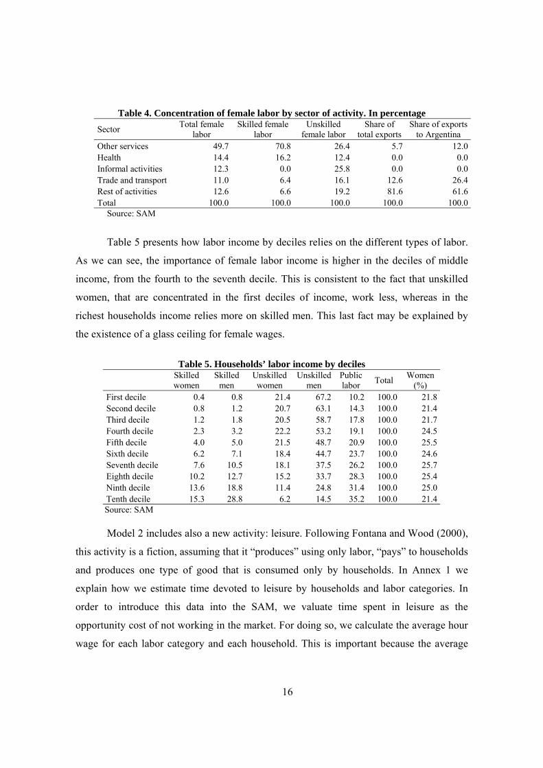
Table 4. Concentration of female labor by sector of activity. In percentage

Sector Total female labor

Skilled female labor

Unskilled female labor

Share of total exports

Share of exports to Argentina

Other services 49.7 70.8 26.4 5.7 12.0Health 14.4 16.2 12.4 0.0 0.0Informal activities 12.3 0.0 25.8 0.0 0.0Trade and transport 11.0 6.4 16.1 12.6 26.4Rest of activities 12.6 6.6 19.2 81.6 61.6Total 100.0 100.0 100.0 100.0 100.0

Source: SAM

Table 5 presents how labor income by deciles relies on the different types of labor.

As we can see, the importance of female labor income is higher in the deciles of middle

income, from the fourth to the seventh decile. This is consistent to the fact that unskilled

women, that are concentrated in the first deciles of income, work less, whereas in the

richest households income relies more on skilled men. This last fact may be explained by

the existence of a glass ceiling for female wages.

Table 5. Households’ labor income by deciles

Skilled women

Skilled men

Unskilled women

Unskilled men

Public labor Total Women

(%) First decile 0.4 0.8 21.4 67.2 10.2 100.0 21.8 Second decile 0.8 1.2 20.7 63.1 14.3 100.0 21.4 Third decile 1.2 1.8 20.5 58.7 17.8 100.0 21.7 Fourth decile 2.3 3.2 22.2 53.2 19.1 100.0 24.5 Fifth decile 4.0 5.0 21.5 48.7 20.9 100.0 25.5 Sixth decile 6.2 7.1 18.4 44.7 23.7 100.0 24.6 Seventh decile 7.6 10.5 18.1 37.5 26.2 100.0 25.7 Eighth decile 10.2 12.7 15.2 33.7 28.3 100.0 25.4 Ninth decile 13.6 18.8 11.4 24.8 31.4 100.0 25.0 Tenth decile 15.3 28.8 6.2 14.5 35.2 100.0 21.4

Source: SAM

Model 2 includes also a new activity: leisure. Following Fontana and Wood (2000),

this activity is a fiction, assuming that it “produces” using only labor, “pays” to households

and produces one type of good that is consumed only by households. In Annex 1 we

explain how we estimate time devoted to leisure by households and labor categories. In

order to introduce this data into the SAM, we valuate time spent in leisure as the

opportunity cost of not working in the market. For doing so, we calculate the average hour

wage for each labor category and each household. This is important because the average

17

hour wage depends not only on the qualification of the worker but also on other variables,

such as the social network of the household.

Model 3 separates leisure activity in leisure and domestic work. Annex 1 also

presents the estimation of time spent in domestic work. In the SAM, domestic work is also

valuated as the opportunity cost of not working in the market.

In terms of market value, time spent in market work, leisure and domestic work is

shown in table 6. It must be noticed that in this case we are not considering time in hours

but time valued at the opportunity cost, and for that reason there are significant differences

with table 23. When we value time spent in labor market, leisure and domestic work

according to the opportunity cost, the share of market work for skilled workers is higher

than the estimations presented in table 2. The opportunity cost for the same category of

worker varies according to the type of household (defined by deciles of income). Skilled

workers in higher income households obtain higher wages and assign more time at market

work. In contrast, skilled workers in lower income household obtain lower wages and

assign more time in leisure and domestic work. Therefore, for skilled workers, total hours

spent in market work are in average valuated at a higher opportunity cost than hours spent

in leisure and domestic work. Despite this, the main conclusions about the time distribution

by gender remain; women spend more time working at home while men spend more time at

market work. Also, unskilled workers spent more time in leisure.

Table 6. Valued time distribution for each labor category

Skilled women Skilled men Unskilled women Unskilled men Market work 34.6 52.2 19.4 39.6 Leisure 41.8 39.3 53.3 51.7 Domestic work 23.6 8.5 27.3 8.7 Total 100.0 100.0 100.0 100.0

Source: SAM

3 Besides, in table 6 time spent in personal care is not considered, and for that reason percentages presented in table 2 are much lower.

18

4. Scenarios and Results

4.1. Simulation scenarios

The aim of this paper is to assess how trade openness affects welfare, relative prices,

specialization, trade and labor market in Uruguayan economy using different specifications

of a CGE model. With that in mind, we simulate three different scenarios. The first one

assumes a complete liberalization of trade with the rest of the world, which implies a null

tariff level for imports coming from the rest of the world. In the base year, trade with

MERCOSUR is already liberalized, and tariffs to imports from Argentina and Brazil are

already zero. Although we are conscious that this scenario is quite extreme and is not

plausible to happen in the short and medium term, we think that it might provide interesting

insights into how trade openness affects labor market by gender and also allows us to

compare the conclusions with the results from other studies.

The second and third scenarios are backwards experiments. They simulate a trade

closure, by setting tariffs at the level of 1994, when trade openness was starting to be

implemented in Uruguay. One of these scenarios simulates the tariff structure of 1994, and

the other one simulates also the existence of reference prices in textiles. Reference prices

act as tariffs, so we simulate the equivalent ad valorem tariffs associated with these prices,

taken from Terra et al (2005). Garments and textiles are female labor intensive, and for that

reason we might expect different results on gender parameters when we introduce reference

prices in these sectors. These two scenarios are analyzed together in order to compare how

reference prices affected labor market in the 1990s. Table 7 presents the tariff structure

applied in 1994 and the tariff structure at the base year (2000) for comparison purposes.

Garments and textiles are considered as “export activities” in the SAM used in this work.

When we introduce an equivalent tariff to reference prices, the tariff applied to import from

the rest of the world for “export activities” increases to 30.5% while the one applied to

import activities increases to 14%.

19

Table 7. Ad valorem tariffs simulated for each sector of activity

Tariff structure in 1994 Tariff structure at base year

Sector of activity (SAM)

Argentina Brazil ROW ROW Agriculture 2.1 2.1 13.7 3.9 Rice 4.5 4.5 17.7 2.4 Ceramics 5.3 5.3 17.6 12.7 Tanning 0.7 0.6 6 0.1 Export activities 6.3 6.4 18.7 12.9 Forestry 0.8 1.1 11.5 7.8 Meat processing 2.5 2.4 15.5 2.0 Husbandry 1.5 1.4 14.2 0.5 Gas 1.7 1.7 15 0.0 Import activities 2.9 2.9 13.9 7.5 Dairy products 5.6 5.6 16.6 3.8 Wood and paper 6.5 6.5 18.2 5.3 Non tradable activities 4.2 4.1 15.2 10.1 Other primary activities 1.1 1.3 12.9 0.2 Chemicals 1.2 1.5 9.3 6.7 Refinery 0.7 1.1 10.7 0.5 Other services 1.1 1.1 13.9 0.0

4.2 Results

In this section we analyze, first, the impact of total trade liberalization on

macroeconomic and labor market variables, and specialization patterns. Then we focus on

the scenarios where trade protection increases.

a. Total trade liberalization

Complete trade openness to the rest of the world has the expected positive impact on

macroeconomic variables. Both exports and imports increase by more than 10 percent.

Meanwhile, real GDP, absorption and investment rise. However, the impact is higher in the

models with endogenous labor supply, especially when we consider Model 3, which also

introduces domestic work. Since exports of Uruguay are relative intensive in labor, trade

liberalization leads to an increase of wages and labor supply. Then, GDP and consumption

possibilities increase more than in a scenario where labor supply is fixed.

20

Table 8. Impact of trade openness on macroeconomic variables. Percentage change

Exogenous labor supply

Endogenous labor supply

Endogenous labor supply and home

production Absorption 0.53 0.54 0.70 Household consumption 0.69 0.69 0.71 Investment 0.16 0.17 1.37 Real GDP 0.78 0.78 0.95 Exports 12.96 12.94 13.28 Imports 10.25 10.24 10.50 Consumer price index -0.13 -0.13 -0.12

Since tariffs applied to imports from MERCOSUR partners are near to zero, trade

liberalization affects mainly tariffs applied to the rest of the world (ROW). Then, imports

from ROW show a significant increase while imports from Argentina and Brazil fall. Table

8 shows that the former increase more than 39% and the latter fall 22% and 25%

respectively. Uruguayan economy benefits from a significant reduction of trade diversion

from MERCOSUR partners. At the same time exports to all destinations increase, but the

rise is higher for Argentina (almost 15%) and Brazil (around 14%) than for the ROW (less

than 12%).

Table 9. Impact of trade openness on trade flows

Model Trade Flow Argentina Brazil Rest of the world

Exports 14.7 13.9 11.4 Exogenous labor supply Imports -22.2 -25.2 39.2 Exports 14.8 13.9 11.4 Endogenous labor supply Imports -22.2 -25.2 39.2 Exports 14.8 14.2 11.9 Endogenous labor supply and

home production Imports -22.1 -25.1 39.5

Table 10 shows relative intensity in the use of factors and balance of trade by

partners for aggregated sectors4. As shown, trade patterns with main commercial partners

differ substantially. Uruguay has a trade surplus with Argentina in services, which are

highly intensive in skilled labor, especially female labor. On the other hand, the country has

4 There are six aggregated sectors: agriculture and agroindustries, which comprise primary activities and food industry; import substitution manufactures, which comprise chemicals, paper and ceramics; exporting manufactures that include textiles, garments and tanning; tradable services that include services to enterprises and tourist services such as transport, hotels and restaurants; non tradable services, which are mainly health and informal activities; and oil and gas.

21

a trade surplus with Brazil and the ROW mainly in agriculture and agroindustries, which

are intensive in unskilled male labor. Importable manufactures present a similar factor

intensity pattern. In this sector Uruguay presents a trade deficit with the three partners.

Table 10. Trade balance and relative intensity in the use of factors of main sectors at

the benchmark

Relative intensity Trade Balance (millions of dollars)

Sector Skilled Female

Skilled Male

Unskilled Female

Unskilled Male Capital ARG BRA ROW Total

Agriculture and agroindustries 0.6 0.8 0.9 1.2 1.0 -9 284 587 862Exporting manufactures 0.5 0.6 1.0 0.7 1.2 10 54 377 441 Import substitution manufactures 0.8 1.0 0.8 1.1 1.0 -383 -322 -1,232 -1,938 Tradable services 1.5 1.4 0.8 0.5 1.1 435 -24 -162 249 Non tradable services 2.6 1.4 2.3 1.3 0.6 - - - - Oil and gas 1.0 1.0 0.6 0.8 1.1 -29 -8 -57 -94 Total 1.0 1.0 1.0 1.0 1.0 23 -16 -487 -480

Source: SAM

As a consequence, the change in trade flows from liberalization leads to a change in

relative factor demand. The increase in exports to the three partners generates an increase in

labor demand and wages for all categories of workers. This happens in the three models, as

shown in table 11, which presents changes in labor market variables. Therefore,

unemployment falls among unskilled workers. Employment and wages increase for both

unskilled and skilled workers, except in Model 1, in which skilled employment does not

change because it is assumed fixed.

Unskilled labor demand increases for both genders, but it increases more for

women. As a consequence, female unemployment falls more. The fall of unemployment

increases wages because firms are willing to increase the wage premium that they pay in

order to promote efficiency among workers. The increase of wages is higher for unskilled

women than for unskilled men. Thus, the gender wage gap falls. The gender wage gap also

falls for skilled workers, because demand for skilled women increases more than demand

for skilled men.

Thus, trade openness reduces the gender wage gap both among skilled and unskilled

workers. At the same time, it widens the wage gap between skilled and unskilled labor.

These two trends can be explained by the changes in trade flows, which lead to changes in

22

relative factor demand. The second trend, the increase in the wage premium, is a

consequence of the higher increase of exports to Argentina, which are intensive in skilled

labor, and the significant rise of imports from the rest of the world, which are intensive in

unskilled male labor. On the other hand, the reduction in the gender gap responds to the fact

that exports to Argentina are more intensive in skilled female labor while imports from the

ROW are more intensive in unskilled male labor. Then, female labor demand increases

more than male labor demand for both skills.

Table 11. Impact of trade openness on unemployment, employment and wages.

Percentage change

Skill Gender Exogenous labor supply

Endogenous labor supply

Endogenous labor supply and home

production

Unemployment Unskilled Female -4.30 -4.35 -4.37 Unskilled Male -4.13 -5.22 -5.48

Employment Total Female 0.18 0.28 0.25

Unskilled Female 0.34 0.32 0.27 Skilled Female 0.00 0.24 0.23

Total Male 0.21 0.17 0.20 Unskilled Male 0.33 0.19 0.24

Skilled Male 0.00 0.14 0.14 Wages

Unskilled Female 0.66 0.67 0.67 Skilled Female 1.01 0.83 0.84 Unskilled Male 0.42 0.54 0.57 Skilled Male 0.94 0.86 0.88

Model 1 does not allow a supply response to the increase in labor demand, as labor

supply is assumed constant. When we introduce an endogenous labor supply in Models 2

and 3, skilled workers increase time spent in the labor market and their wages increase less

than in the previous model. The effect is particularly important among skilled women. This

situation is illustrated in figure 3. The initial equilibrium locus of wages and employment is

represented by point A. When assuming fixed labor supply, the increase in labor demand

leads to an increase of wages from A to B. In contrast, in Models 2 and 3, labor supply

increases with wages. Thus, a shift of the demand means a movement from A to B’.

Additionally, the increase of the income of the rest of the household, originated on the rise

23

of wages and employment, produces a reduction of labor supply. Therefore, the final

equilibrium is reached in C, where employment, labor supply and wages are higher than in

A.

Figure 3. Changes in skilled labor market according to model 1 and 2

In the case of unskilled labor, trade liberalization also increases labor demand but

the changes in labor market cannot be explained with the same figure, because we are

assuming a wage curve specification. Compared to Model 1, wages increase slightly more

because unemployment falls more. The fall of unemployment is higher for unskilled men

than women, because men reduce labor supply more than women. Their behavior is

consistent with an increase of their household income originated in the rise of wages and

employment of unskilled labor. This effect outstrips a potential increase of labor supply

originated by the rise of their wages.

Table 12 shows the change in the use of time by worker categories. Skilled workers

increase labor market supply and reduce time spent in domestic work and leisure, which is

consistent with the rise of their wages. The behavioral reaction is deeper among women.

Specifically, their increase in the labor market supply is quite higher than for men.

Unskilled workers behave differently. Both men and women reduce their labor market

offer, because, as already explained, total income of the household increases. As a

consequence, unskilled workers increase leisure and domestic work, but the effect is more

important for men.

L0 LC LB’

wB wc wB’ wA

A

D’

D S1

B’

B

Labour

Wage

Labour

Wage

S’1

S0

C

24

Assuming that households are composed by men and women of the same skill, trade

openness generates an intra-household time reallocation, making men dedicate more time to

domestic work activities and thus improving equity within households. In spite of this,

skilled women lose a high percentage of leisure time.

Table 12. Impact of trade openness on time distribution for each labor category.

Percentage change. Model with endogenous labor supply and domestic work

Labor supply

Leisure time

Time spent in domestic work

Skilled female workers 0.23 -0.13 -0.10 Skilled male workers 0.14 -0.16 -0.12 Unskilled female workers -0.08 0.02 0.01 Unskilled male workers -0.19 0.13 0.09

Under a trade openness scenario, all types of households increase their income

(table 13). The richest households are the most benefited. This is a result of the relative

increase of skilled wages and employment. Imports increase mainly in sectors intensive in

capital and unskilled labor while exports increase more in sectors intensive in skilled labor.

Although this would be a rough measure of income distribution we can say that trade

openness could likely generate a general welfare improvement but at the same time it

would increase inequality.

Table 13. Households’ income variation. Percentage change

Exogenous labor supply

Endogenous labor supply

Endogenous labor supply and home

production

First decile 0.64 0.64 0.66 Second decile 0.66 0.65 0.67 Third decile 0.66 0.65 0.67 Forth decile 0.68 0.68 0.70 Fifth decile 0.69 0.69 0.70 Sixth decile 0.68 0.68 0.70 Seventh decile 0.67 0.67 0.69 Eighth decile 0.67 0.67 0.69 Ninth decile 0.69 0.70 0.71 Tenth decile 0.73 0.74 0.74

25

b. Backwards experiments

The backwards experiments may be useful to test which of the stylized facts of the

Uruguayan economy and labor market from 1994 to 2000 can be explained by trade

openness to the region and the world. Under this scenario, we simulate an increase in tariffs

applied to imports from the three partners, but tariffs are higher for imports from the ROW,

as already shown in table 7.

Table 14 shows that the increase in protection has the opposite effect on

macroeconomic variables compared to the trade openness scenario. Tariffs increase more

for imports from the ROW, and then imports fall, mainly from this origin.

Table 14. Impact of trade protection on macroeconomic variables. Percentage change.

Exogenous labor supply

Endogenous labor supply

Endogenous labor supply and home

production Tariff structure in 1994 Absorption -0.48 -0.41 -0.59 Household consumption -0.55 -0.49 -0.51 Investment -0.57 -0.32 -1.66 Real GDP -0.70 -0.62 -0.81 Exports -13.12 -13.09 -13.43 Imports -10.55 -10.52 -10.80 Consumer price index 0.11 0.12 0.10

The impact on labor market is also the opposite than under the trade openness

scenario (see table 15). Labor demand decreases for all categories of workers, especially for

men. Unemployment rises, employment decreases and wages go down. However, labor

supply increases in the models where it is assumed to be endogenous. This happens because

the fall in wages reduces the household’s income; then the positive effect on labor supply

prevails over the negative impact of wages. As a consequence wages fall more than in the

fixed labor supply model.

In the case of unskilled labor, unemployment increases more, both for men and

women. Because there is no unemployment among skilled workers, the rise in labor supply

leads to an increase in employment but a deeper fall in wages. This is particularly important

for women whose labor supply increases more. As a consequence the gender gap increases,

especially for skilled women.

26

Table 15. Impact of trade protection on unemployment, employment and wages. Percentage change. Tariff structure of 1994

Skill Gender Exogenous labor supply

Endogenous labor supply

Endogenous labor supply and home

production

Unemployment Unskilled Female 2.82 3.15 3.23 Unskilled Male 4.42 4.46 4.86

Employment Total Female -0.12 0.11 0.14

Unskilled Female -0.23 -0.11 -0.05 Skilled Female 0.00 0.35 0.35

Total Male -0.22 -0.05 -0.09 Unskilled Male -0.35 -0.26 -0.32

Skilled Male 0.00 0.29 0.28 Wages

Unskilled Female -0.42 -0.46 -0.48 Skilled Female -0.09 -0.30 -0.31 Unskilled Male -0.43 -0.44 -0.47 Skilled Male -0.02 -0.17 -0.20

Table 16 shows what we have already explained: the rise of labor supply, especially

among skilled workers. Unskilled female workers increase time spent in labor market more

in the experiment with reference prices, because of the increase in unskilled female labor

demand in the protected sector. Time spent in domestic work falls for all types of labor

categories, deepening the negative impact of the wage fall.

Table 16. Change in the use of time for each labor category

Tariff structure of 1994

Labor supply Leisure time Time spent in

domestic work Skilled female workers 0,35 -0,19 -0,17 Skilled male workers 0,28 -0,31 -0,26 Unskilled female workers 0,19 -0,04 -0,05 Unskilled male workers 0,07 -0,04 -0,06

Lastly, we can see in table 17 that income falls for all types of households, but falls

more among the richest households, especially in the first specification of the model,

because employment among skilled workers is considered as fixed.

27

Table 17. Households’ income variation. Percentage change

Exogenous labor supply

Endogenous labor supply

Endogenous labor supply and home production

Tariff structure in 1994 plus reference prices in textiles First decile -0,50 -0,48 -0,51 Second decile -0,54 -0,51 -0,53 Third decile -0,54 -0,50 -0,53 Forth decile -0,58 -0,53 -0,56 Fifth decile -0,58 -0,53 -0,55 Sixth decile -0,56 -0,51 -0,53 Seventh decile -0,52 -0,47 -0,49 Eighth decile -0,50 -0,45 -0,47 Ninth decile -0,52 -0,46 -0,48 Tenth decile -0,59 -0,52 -0,53

When we simulate an additional increase in protection due to the introduction of

reference prices for textiles and garments, the macroeconomic impact is very similar to the

results presented in table 14, but deeper. Table 18 presents the impact on labor market. It

should be noted that the introduction of references prices in order to protect female

employment (textiles and garments) does not contribute to improve female conditions in

labor market. On the contrary, female wages fall more than male ones, because the sectors

that are being protected are export sectors, and even when protection does reduce import

competition, the negative impact on exports is even higher when the policy is implemented.

Table 18. Impact of trade protection on unemployment, employment and wages.

Percentage change. Tariff structure of 1994 plus reference prices in textiles and garments

Skill Gender Exogenous labor supply

Endogenous labor supply

Endogenous labor supply and home

production Unemployment

Unskilled Female 2.83 3.31 3.37 Unskilled Male 4.76 4.79 5.20

Employment Total Female -0.12 0.11 0.15

Unskilled Female -0.23 -0.09 -0.02 Skilled Female 0.34 0.34

Total Male -0.24 -0.07 -0.12 Unskilled Male -0.12 -0.29 -0.35

Skilled Male 0.28 0.26 Wages

Unskilled Female -0.42 -0.49 -0.50 Skilled Female -0.13 -0.34 -0.35 Unskilled Male -0.46 -0.47 -0.51 Skilled Male -0.08 -0.22 -0.25

28

5. Sensitivity analysis

Results obtained may be sensitive to changes in some of the parameters adopted in the

study. In order to test how sensitive results are, we run three different sensitivity analyses

and a new backwards scenario that simulates the break of MERCOSUR agreement through

an increase in tariffs applied to imports from MERCOSUR countries.

5.1. Changes in elasticity of substitution by gender in the production function

In the model, the elasticity of substitution among men and women in the production

function of all products is the same, at the value of 1.1. However, it may be assumed that in

some sectors the substitution among men and women is more imperfect, such as in the

construction sector, where only 6 percent of workers are women. Therefore, we run a

sensitivity analysis allowing the value of the elasticity of substitution among men and

women in the production function to vary among sectors. Even though there is no

estimation of this elasticity, we assume that sectors that at the benchmark present a high

intensity in the use of male or female labor (over 80 percent) present an imperfect

substitution among labor by gender and the elasticity was set at 0.1. Then, other sectors

present a medium intensity (between 70 and 80 percent), and the elasticity was set at 0.3.

Finally, sectors that hire both male and female labor maintain the elasticity value of 1.1.

Table 19 shows the values adopted for each sector.

Table 19. Elasticity of substitution among workers by gender

Elasticity of substitution Low Medium High

Agriculture, Husbandry, Forestry, Other primary,

Wood and paper, Ceramics, Construction,

Refinery, Import activities

Meat processing, Dairy products, Rice,

Tanning, Non tradable activities, Gas, Trade

and transport

Chemicals, Export activities, Hotels and restaurants, Health,

Other services, Informal activities

Table 20 shows the impact of trade openness in Model 3 (endogenous labor supply and

home production) on employment and wages when the elasticity of substitution by gender

varies among sectors. We can see that there are no significant differences with the results

presented in the previous section. Although female employment increases more and male

29

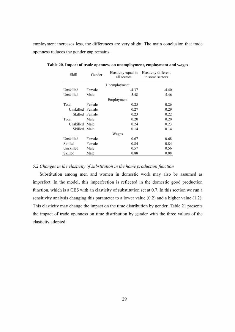
employment increases less, the differences are very slight. The main conclusion that trade

openness reduces the gender gap remains.

Table 20. Impact of trade openness on unemployment, employment and wages

Skill Gender Elasticity equal in all sectors

Elasticity different in some sectors

Unemployment Unskilled Female -4.37 -4.40 Unskilled Male -5.48 -5.46

Employment Total Female 0.25 0.26

Unskilled Female 0.27 0.29 Skilled Female 0.23 0.22

Total Male 0.20 0.20 Unskilled Male 0.24 0.23

Skilled Male 0.14 0.14 Wages

Unskilled Female 0.67 0.68 Skilled Female 0.84 0.84 Unskilled Male 0.57 0.56 Skilled Male 0.88 0.88

5.2 Changes in the elasticity of substitution in the home production function

Substitution among men and women in domestic work may also be assumed as

imperfect. In the model, this imperfection is reflected in the domestic good production

function, which is a CES with an elasticity of substitution set at 0.7. In this section we run a

sensitivity analysis changing this parameter to a lower value (0.2) and a higher value (1.2).

This elasticity may change the impact on the time distribution by gender. Table 21 presents

the impact of trade openness on time distribution by gender with the three values of the

elasticity adopted.

30

Table 21. Impact of trade openness on time distribution of workers, with different

elasticity of substitution value in the domestic production function

Labor supply Leisure time

Time spent in domestic

work Elasticity = 0,2

Skilled female workers 0.21 -0.15 -0.05 Skilled male workers 0.13 -0.17 -0.06 Unskilled female workers -0.07 0.02 0.01 Unskilled male workers -0.18 0.13 0.03

Elasticity = 0,7 Skilled female workers 0.23 -0.13 -0.10 Skilled male workers 0.14 -0.16 -0.12 Unskilled female workers -0.08 0.02 0.01 Unskilled male workers -0.19 0.13 0.09

Elasticity = 1,2 Skilled female workers 0.24 -0.12 -0.14 Skilled male workers 0.15 -0.16 -0.18 Unskilled female workers -0.08 0.02 0.02 Unskilled male workers -0.19 0.12 0.15

Trade openness increases skilled female labor demand and wages, and skilled women

are tempted to increase labor supply. However, when the substitution in the domestic good

production among genders is more imperfect, skilled women increase labor supply less, and

they are not able to reduce time spent in domestic work as much as they would like. In

order to increase time spent in labor market, they must reduce leisure time. A more perfect

substitution of workers by gender in the home production function also benefits unskilled

women, because unskilled men increase more time spent in household activities under this

assumption.

5.3. Maximum time available for work, domestic work and leisure

In the model we assume that the maximum time available for work, domestic work and

leisure is 14 hours per day for both genders. The rest of the hours of the day are supposed to

be the minimum necessary for sleep, eat, etc. We might assume however that women count

with fewer hours to freely distribute between the different activities, because of the rigidity

of some tasks at home, such as childcare, eldercare, etc. In order to assess the impact of this

gender rigidity at home, we assume that women count with fewer hours per day to work at

31

labor market, at home and to spend in leisure activities, setting the maximum time available

for women at 10 hours.

Results on time distribution are, as expected, particularly important among women.

When skilled women face a restriction on the maximum available hours to spend in the

three activities, they increase time spent in labor market, but less. Leisure time and

domestic time fall more because the original amount of hours at the base year is lower. On

the other hand, unskilled female workers reduce labor supply less, while they increase more

time spent in leisure and in domestic activities.

Table 22. Impact of trade openness on time distribution of workers, with different availability

of hours per day for women and men

Labor supply Leisure time

Time spent in domestic

work MAXHS= 10 (WOMEN)

Skilled female workers 0.17 -0.18 -0.13 Skilled male workers 0.14 -0.16 -0.12 Unskilled female workers -0.06 0.03 0.02 Unskilled male workers -0.19 0.13 0.09

MAXHS= 14 Skilled female workers 0.23 -0.13 -0.10 Skilled male workers 0.14 -0.16 -0.12 Unskilled female workers -0.08 0.02 0.01 Unskilled male workers -0.19 0.13 0.09

5.4. Break of MERCOSUR agreement

Trade openness scenario simulates liberalization only with the ROW, because in the

benchmark tariffs to MERCOSUR imports are already zero. Therefore, we cannot simulate

the gender-differentiated effects on employment, wages and time allocation of

liberalization with MERCOSUR partners. In this section we present results of a new

backwards experiment, which simulates an increase of tariffs to MERCOSUR partners,

using the same tariff structure at the benchmark applied to imports from the rest of the

world. In order to analyze the effects of trade openness with MERCOSUR partners, signs

obtained should be interpreted as the opposite.

Table 23 presents the impact on trade by partner. We can expect that trade liberalization

with MERCOSUR partners leads to a high increase of trade with the region, reducing

imports from the ROW.

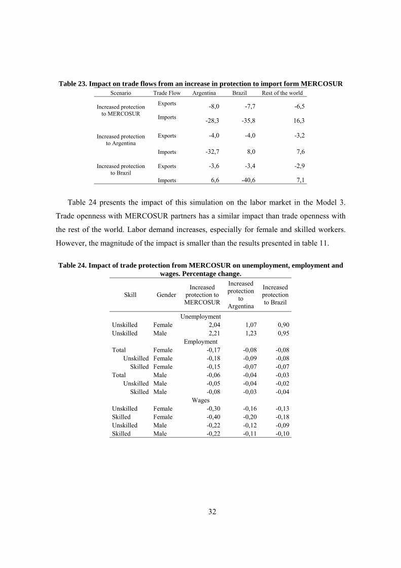
32

Table 23. Impact on trade flows from an increase in protection to import form MERCOSUR

Scenario Trade Flow Argentina Brazil Rest of the world

Exports -8,0 -7,7 -6,5 Increased protection to MERCOSUR Imports -28,3 -35,8 16,3

Exports -4,0 -4,0 -3,2 Increased protection to Argentina

Imports -32,7 8,0 7,6

Exports -3,6 -3,4 -2,9 Increased protection to Brazil

Imports 6,6 -40,6 7,1

Table 24 presents the impact of this simulation on the labor market in the Model 3.

Trade openness with MERCOSUR partners has a similar impact than trade openness with

the rest of the world. Labor demand increases, especially for female and skilled workers.

However, the magnitude of the impact is smaller than the results presented in table 11.

Table 24. Impact of trade protection from MERCOSUR on unemployment, employment and

wages. Percentage change.

Skill Gender Increased

protection to MERCOSUR

Increased protection

to Argentina

Increased protection to Brazil

Unemployment Unskilled Female 2,04 1,07 0,90 Unskilled Male 2,21 1,23 0,95

Employment Total Female -0,17 -0,08 -0,08

Unskilled Female -0,18 -0,09 -0,08 Skilled Female -0,15 -0,07 -0,07

Total Male -0,06 -0,04 -0,03 Unskilled Male -0,05 -0,04 -0,02

Skilled Male -0,08 -0,03 -0,04 Wages

Unskilled Female -0,30 -0,16 -0,13 Skilled Female -0,40 -0,20 -0,18 Unskilled Male -0,22 -0,12 -0,09 Skilled Male -0,22 -0,11 -0,10

33

6. Concluding remarks

In the 1990s the Uruguayan economy deepened trade openness. At the same time a

reallocation of employment towards services sector, an increase in wage gap by skill, an

increase of unemployment and informality took place. Female participation in labor market

grew and discrimination increased.

In this paper we analyze the gender differentiated impacts of trade openness in

Uruguay using a gender aware CGE model. Two main simulations were implemented.

First, complete trade liberalization eliminating tariffs with the rest of the world. Second, a

backward experiment that sets tariff to the level of 1994.

Trade liberalization improves women situation in terms of employment and wages.

This is consistent with Çagatay (2001) and Fofana et al (2003), who conclude that trade

openness has a positive impact on female employment in semi-industrialized countries. The

gender wage gap is reduced among skilled workers and unskilled workers. Additionally, the

premium for education increases. Skilled workers are most benefited because exports to

Argentina, which are intensive in this factor, increases more than exports to other partners.

Among skilled workers, female employment and wages increase more. Unskilled women

are also better off than unskilled men.

These results are consistent with some of the stylized fact mentioned before. Trade

liberalization increases demand of skilled and female labor. However, the model shows a

decrease of unemployment while in facts it grew. This inconsistence shows one limitation

of our model, which does not consider changes in technology. In fact, in the 1990s there

was a strong increase in productivity in Uruguay, which was partly due to an unskilled

labor saving technological change.

The paper also shows that it is important to introduce endogenous labor supply in

the model. When doing so, some of the results obtained in the model with a fixed labor

supply vary. The increase in labor supply provoked by the increase in wages for skilled

workers generates a lower increase in wages. On the contrary, unskilled workers reduce

labor supply, which leads to a higher decrease in unemployment and a higher increase in

wages.

The effect of trade openness on time distribution of workers is different by skills.

When wages increase, skilled workers reduce time spent in leisure and domestic work,

34

because they increase time spent in labor market. The reduction of leisure time is higher for

women than for men. On the contrary, unskilled workers increase leisure time, especially

men. For both skilled and unskilled workers, trade openness leads to a more equitable

distribution of time spent in domestic work. However, when there is a more imperfect

substitution among genders in the home production function, trade liberalization leads to an

increase in skilled female labor supply at the expense of a higher reduction in leisure time.

The simulation of a backwards experiment that sets the tariff structure of 1994 has

the opposite results than the trade openness scenario: employment and wages go down,

unemployment increases and the gender wage gap increases for both skills. These results,

with a higher magnitude, are similar to results obtained when we simulate a breaking of

MERCOSUR agreement.

We also show that a specific policy to protect a female intensive sector, the

introduction of reference prices in female intensive sectors, has a negative effect on female

wages and employment, because of its negative impact on exports.

Our results should be treated carefully, because the sectoral aggregation of our SAM

does not allow considering separately those sectors that present more segregation by

gender, specially garments, textiles and domestic service.

35

References

Aguirre, Rosario and Karina Batthyány (2005). “Trabajo no remunerado y uso del tiempo. Encuesta en Montevideo y área metropolitana 2003”, UNIFEM, UdelaR, Montevideo. Amarante, Verónica (2001). “Diferencias salariales entre trabajadores del sector público y privado”, Serie Documentos de Investigación, DT 2/01, Instituto de Economía, Facultad de Ciencias Económicas y de Administración, UdelaR. Amarante, Verónica and Alma Espino (2001). “La evolución de la segregación laboral por sexo en Uruguay. 1986-1999”, Documento de Trabajo 3/01, Instituto de Economía, Facultad de Ciencias Económicas y de Administración, UdelaR. Armington, P.S. (1969). “A theory of demand for products distinguished by place of production”, IMF Staff Papers, vol. 16, 159-176. Blanchflower, David and Andrew Oswald (1994): The wage curve, Cambridge and London: the MIT Press. Bucheli, Marisa (2002). “Una aproximación al efecto del trabajador añadido”, LC/MVD/R.195, Oficina de CEPAL de Montevideo. Bucheli, Marisa and Graciela Sanromán (2005). “Salarios femeninos en Uruguay: ¿existe un techo de cristal?”, Revista de Economía Vol 12, Nº 2, Segunda Epoca, Banco Central del Uruguay. Çagatay, Nilüfer (2001). “Trade, Gender and Poverty”, Background paper, United Nations Development Programme, Trade and Sustainable Human Development Project. Casacuberta, Carlos and Marcel Vaillant (2004). “Trade and wages in Uruguay in the 1990’s”, Revista de Economía, Banco Central del Uruguay, Volumen 11, Número 2, Segunda Época, november. De Soria Ximena; Fernanda Rivas & Mariana Taboada (2001). “Oferta laboral de las mujeres”. Documento No. 18/01, Departamento de Economía, Facultad de Ciencias Sociales, Universidad de la República, Uruguay. Diez de Medina, Rafael (1992). “El sesgo de selección en la actividad de jóvenes y mujeres”. Documento No. 12/92, Departamento de Economía, Facultad de Ciencias Sociales, Universidad de la República, Uruguay. Fofana, Ismaël, John Cockburn and Bernard Décaluwé (2003). “Modeling male and female work in a computable general equilibrium mode applied to Nepal”, PEP Network training material, Université Laval. Fofana, Ismaël, John Cockburn, Bernard Décaluwé, Ramos Mabugu and Margaret Chitiga (2005). “Does Trade Liberalization Leave Women Behind in South Africa? A Gender CGE

36

Analysis”, Presented in the 4th PEP Research Network General Meeting, Colombo, Sri Lanka, June. Fontana Marzia (2001). "Modelling the effects of trade on women: a closer look at Bangladesh", IDS Working Paper No 139. Fontana, Marzia (2003). “The gender effects of trade liberalization in developing countries: a review of the literature”, Discussion Papers in Economics DP 101, University of Sussex, October. Fontana, Marzia and Adrian Wood, (2000). “Modeling the effects of trade on women at work and at home”, World Development, vol. 28, Nº 7. Harris, Richard (1984), “Applied General Equilibrium Analysis of Small Open Economies with Scale Economies and Imperfect Competition,” American Economic Review, 74(5), December, 1016-1032. Laens, Silvia and Inés Terra (1999). “Effects of the completition of MERCOSUR on Uruguayan labor market. A simulation exercise using a CGE model”, Documento de Trabajo 21/99, Departamento de Economía, Facultad de Ciencias Sociales, UdelaR. Laens, Silvia and Inés Terra (2000): “Efectos del perfeccionamiento del MERCOSUR sobre el mercado de trabajo de Uruguay: un ejercicio de simulación usando un modelo CGE”, Revista de Economía, Banco Central del Uruguay, 7 (2), segunda época, November. Rivas, Fernanda and Máximo Rossi (2000). “Discriminación salarial en el Uruguay 1991-1997”, Documento de Trabajo Nº 7/00, Departamento de Economía, Facultad de Ciencias Sociales, UdelaR. Rivas, Fernanda and Máximo Rossi (2002). “Evolución de las diferencias salariales entre el sector público y el sector privado en Uruguay”, Documento de Trabajo Nº 2/02, Departamento de Economía, Facultad de Ciencias Sociales, UdelaR. Siddiqui, Rizwana (2007). “Modelling Gender Dimensions of the Impact of Economic Reforms in Pakistan”, MPIA Working Paper 2007-13, PEP. Terra, Inés, Gustavo Bittencourt, Rosario Domingo, Carmen Estrades, Gabriel Katz, Alvaro Ons and Hector Pastori (2005). “Estudios de competitividad sectoriales. Industria manufactura”, Documento de Trabajo Nº 23/05, Departamento de Economía, Facultad de Ciencias Sociales, UdelaR. Terra, Inés, Marisa Bucheli, Silvia Laens and Carmen Estrades (2006). “The Effects of Increasing Openness and Integration to the MERCOSUR on the Uruguayan Labor Market: A CGE Modelling Analysis”, MPIA Working Paper 2006-06, PEP.

37

Annex 1: The estimation of the distribution of time

Information about the time devoted to home production is available in a unique time

use survey EUS (Encuesta sobre Uso del Tiempo y Trabajo No Remunerado) carried out by

the Department of Sociology of the FCS-UdelaR. The survey was collected over four

months in 2003 in the city of Montevideo and its metropolitan area. This region

concentrates 59% of the urban population that in turn is 95% of total population.

The observation unit is the household and the sample size is 1.200 households. The

respondent is the person responsible of the household tasks: 84% of the respondents are

women and 16% are men. Aguirre & Batthyány (2005) present more information about the

characteristics the survey and analyze the main results.

The survey inquires about several personal characteristics of the members of the

household, such as the relationship with the respondent, sex and age. A set of questions

collects information about characteristics of the labor market participation of all the

members: hours of work, commuting time, occupation, etc. The most important feature of

the survey is that it seeks to identify and quantify the main types of labor that people over

14 years old engage. The questionnaire offers a list of tasks and the respondent has to

inform the time spent in each task the week previous the interview. Additionally, she has to

report the distribution among the household members of the whole time spent in each task.

Notice that this second question is asked only when the respondent actually does the task.

In order to estimate time spent in domestic work, we consider the following tasks: to

buy food and home furnishing; to take care of pets and plants; to organize and distribute

household tasks; several tasks related to child care (to feed children, to take them to school,

to play with them, to help them with their homework, to bath them, to make them sleep); to

take care of the elder (to help them in many way, to give them their medicines and to

accompany them). We do not include some tasks because its low frequency: to buy and

mend clothes; to repair the house or home furnishings; to go to do some errands for the

home.

The time spent in each task is collected in a table. The tasks appear in the rows and

the columns distinguish the members of the household. As just one column is used for the

children of the respondent, it is not possible to know the sex of every person. Specifically,

there is a problem when the respondent has at least two children of different sex. In these

38

cases we assign the average of time to each child older than 14 years old. As there is also

only one column to report information about the mother and mother-in-law of the

respondent, we proceed analogously. The same happens with the father and father-in-law.

Another disadvantage of the data is that the survey does not inquire about the time

distribution of the tasks that the respondent does not do. Thus, each task that is

responsibility of another member of the household is not considered. As 84% of the

respondents are women, we may expect to observe missing information about time

distribution of tasks traditionally considered “male tasks”. This appears to be the case of

“repairing the house or home furnishing” which consequently has been dropped of the

instrumental definition of domestic work.

The calibration of the CGE model requires disaggregating domestic work between

categories that take into account sex, education and income of the household. As the EUS

does not inquire about the last two variables, we assigned the information about domestic

work provided by this survey to the Household Survey (ECH) microdata collected in 2001

by INE. Notice that we use the ECH of 2001 for the calibration of other CGE model

variables. We pursue the following procedure. First, we fit a model based on the individual

EUS data to explain the time spent on domestic work. Then, then we apply the estimated

coefficients to microdata of the ECH.

In order to estimate the coefficients we use a Generalized Lineal Model. The

dependent variable is the amount of time spent on domestic work by the individual. The

independent variables are chosen between the set of potential determinants that are

collected both in the EUS and the ECH.

The explanatory variable are: i) a dummy variable that takes value 1 when the

individual works in the labor market; ii) the amount of hours spent in the labor market the

week previous to the interview; iii) the age and its square; iv) a dummy variable that takes

value 1 if there is a woman (other than the individual) older than 13 years old; v) a

privation indicator; vi) size of the household; vii) number of household members less than

14 years old. The privation indicator stems from a privation index that weights the lack of

some condition that reflects a lack of status. Among the plausible conditions to be

considered, we choose a set of goods whose possession is collected in both EUS and ECH:

water-heater; heater; fridge; television set in colors; pay channel television; washing

39

machine; dishwasher; microwave owen; personal computer; access to internet; car of

personal use; telephone. The weights reflect that the highest the percentage of people who

possess the good, the highest the feeling of privation -thus, the highest the privation index-.

We fit a model for men and a model for women. The results appear in Table A1.

Table A1. Results of the GLM estimation. Dependent variable: time spent in

domestic work.

Women MenWorker (value 1 if worker) -13,057 ** 3,534

4,143 3,378Hours spent in labor market -0,011 -0,180 *

0,096 0,053Age 3,083 * 1,543 *

0,272 0,251Age squared -0,032 * -0,017 *

0,003 0,003Another women (a) -19,484 * -45,508 *

2,710 9,680Privation index 10,051 ** 1,030

4,080 3,082Household size -4,359 * -4,971 *

0,839 0,445Number of members less than 14 years old 2,381 ** 0,820

1,049 0,974Constante -1,908 47,731 *

5,913 11,285(a) Takes value 1 if there is a woman (other than the individual) older than 13 years old* 99%; ** 95%

40

Annex 2: Core model and calibration of parameters

The CGE model is based on Terra et al (2006). Its structure is quite conventional in

terms of the analysis of trade-related issues but we work with alternative specifications

regarding the labor market in order to take into account gender issues. Specifically, we use

three different versions of the model: first, we disaggregate male and female labor demand

(model 1), second, we consider male and female labor supply as endogenous (model 2) and

third, we incorporate domestic work in the model (model 3).

The main features of the CGE model (model 0) are:

• It is a multi-sector model, including two special cases. In one of them we assume

that employment and wages are fixed: this sector gathers all the activities in which

institutional arrangements and/or trade unions are a deterrent to workers’ dismissal

or to wage reductions (mainly, public services and the financial sector). The other

one consists on an informal sector that produces one type of good destined only to

domestic final consumption.

• We assume that Uruguay has three trading partners (Argentina, Brazil and the rest

of the world). The Uruguayan economy is explicitly modeled while in the case of

the other trading partners only the supply of imports and the demand for exports are

endogenous.

• Perfect competition is assumed in all sectors. However, goods are not homogenous,

as they are differentiated by geographic origin.

• We assume that there are ten representative households which represent different

income levels (by deciles of the income distribution).

• Government collects tariffs and taxes. Government revenue is used to buy goods

and services and to make transfers to households. We assume that government has

fixed consumption of goods and services (in physical units) and the transfers to

households are updated by the change in the average wage. Government savings is

obtained as a residual.

• On the production side, the study uses a nested production function. At the top

level, firms combine intermediate inputs with value added following a Cobb-

Douglas function. Value added is obtained with a constant elasticity of substitution

(CES) function that combines capital and composite labor. Then, composite labor is

41

obtained by combining skilled and unskilled labor with a CES. In the informal

sector, value added is only composed by unskilled labor.

• Goods are imperfect substitutes in consumption (Armington). The small country

assumption is made for imports, so the country faces a perfectly elastic supply curve

in the external markets. However, it is assumed that the country faces a downward

sloping demand curve for exports (quasi small open economy)5. Export demand is a

function of relative prices and real income in the trade partners, which are

considered exogenous.

• Total demand for each sector is composed by domestic demand (intermediate and

final) plus exports to each of the trading partners.

• Trade balance is fixed so imports and exports of goods and services maintain the

benchmark data’s difference. The equilibrium in the model is defined by the

simultaneous equilibrium in goods and factor markets and in the external sector.

• There are three factors of production: capital, skilled labor and unskilled labor (in

further specifications of the model labor market is also segmented by gender). The

supply of each factor is fixed and there is no international mobility. Skilled labor is

employed only in the formal sector. Unskilled labor may be employed in the formal

or the informal sector.

• Unemployment is fixed.

• The model was run using GAMS (General Algebraic Modeling System).

Equations

First we present all the equations of the basic model (model 0). Then we will

specify the main characteristics of the three versions of the model:

Model 1: Disaggregating labor demand by gender

Model 2: Endogenous labor supply and leisure

Model 3: Endogenous labor supply and domestic work

5 Following Cox’s specification (1994).

42

Lower fonts indicate endogenous variables, capital fonts refer to exogenous

variables and Greek letters indicate parameters. The subscripts i, j refer to sectors, the

subscripts z, t refer to geographic zones, the subscripts f refer to representative households

grouped according to income levels, the subscripts k refer to f plus government and the

subscript h refers to factors of production as follows:

i, j = {1, 2, …, J}

z = {Uruguay (u), Argentina (a), Brazil (b), rest of the world (r)}

t = a, b, r

f = (f1, f2, f3, f4, f5, f6, f7, f8, f9, f10)

K = (f1, f2, f3, f4, f5, f6, f7, f8, f9, f10, g)

H = (SL, NSL, CAP)

Where SL refers to skill labor, NSL refers to unskilled labor and CAP refers to

capital.

We can define a subset LAB of factors H:

LAB = (SL, NSL)

1. Demand Structure

Demand functions are derived from a Cobb Douglas utility function which is an

increasing function of consumption of composite goods that combines different varieties of

differentiated goods. In turn, the sub-utility functions follow an Armington specification

(1969) in perfect competition sectors. In the perfectly competitive sectors, goods are

differentiated by geographic origin.

Consumers maximize a Cobb Douglas utility function subject to their budget

constraint. As such, demand for each good is stated thus:

i

fffifif pf

msavtdyc

)1)(1(.

−−= μ (1)

where cif is the demand for a composite final good i (differentiated by geographic

origin), yf is the total income of a representative household f in Uruguay, tdf is the direct

tax rate, msavf is the marginal propensity to save and pfi is the composite price index. This

index can be written as:

43

( ))1/(1

1i

ii

zzizii ppf

φφφλ

−− ⎟

⎠

⎞⎜⎝

⎛= ∑ (2)

being λzi the share parameter in the Armington function, Фi the elasticity of

substitution between goods from different origin and pzi the market price of good i from

market z.

Investment demand of good i is a fixed share of total investment I:

(3)

Final demand of a differentiated good i produced in country z by an institution k is:

kii

zizizik c

pfpd

i

i ..φ

φλ−

⎟⎟⎠

⎞⎜⎜⎝

⎛= (4)

where dzik is the final domestic demand of institution k.

The export demand for a representative domestic firm is a decreasing function of the

export price:

0 . ..

i

i

iz iz tiz

zi

e p ReER pd

η

η

−

−= (5)

where eiz is the demand for a variety of the differentiated good i in market z, piz is

the export price from Uruguay, pdzi is the domestic price index of good i in market z, Rt is

the real income of the partner t, ER is the exchange rate and eoiz is a parameter.

2. Production

Each sector combines primary factors and intermediate inputs following a Cobb-

Douglas production function. The value added is a nested CES production function

combining skilled labor, unskilled labor and capital.

3. Cost

Total variable cost is derived from a Cobb-Douglas constant return to scale

production function. The variable unit cost is:

( )( ) ∏∑+= −

jjiiiii

jij

ji vitindvcv ααω .1 1 (6)

iiinviinv pf

Ic μ=

44

where vi is the variable unit cost, vci is the value added cost and viij is the composite

price of intermediate inputs. αij is the distribution parameter of a Cobb-Douglas production

function, tindi is the value added tax rate and ωi is a parameter.

In turn, value added is a combination of labor and capital specified as a CES. Thus,

vci is:

( )[ ] )1/(1)1()1( ..1 iiiiiiiii wrvc σσσσσ δδ −−− +−= (7)

where ri and wi,, are the rental rate of capital and the average wage, δ is the

distribution parameter of the CES function for value added, while σi is the elasticity of

substitution between capital and labor.

As the model considers two types of labor, the average wage is a combination of

skilled and unskilled wage. It is assumed that skilled labor and unskilled labor are

combined following a CES function, so the average wage is:

( ) ( )[ ] )1/(111 ..1.1 iiiii wswuw iii

i

θθθθθ ξξϕ

−−− +−= (8)

where wi is the average wage, wui and wsi are the unskilled and the skilled wages,

respectively, ξ and ϕ are the distribution and scale parameters, and θi is the elasticity of

substitution between skilled and unskilled labor.

The intermediate inputs are differentiated by geographic origin with an Armington

formulation. The composite price of intermediate inputs is:

( ))1/(1

1.j

jj

zzjzjiji pvi

φφφγ

−− ⎟

⎠

⎞⎜⎝

⎛= ∑ (9)

where pzj is the price in the local market of input j used in sector i in each zone, γzji

is the CES distribution parameter and φj is the elasticity of substitution between goods from

different origins.

4. Input and factor demand by firm

Firms maximize their profits so demand for intermediate inputs and value added

(labor and capital) in each sector is obtained from their maximization program: j

jizji

zj

ji

ijizji vi

pvi

vx

φ

γα

−

⎟⎟⎠

⎞⎜⎜⎝

⎛=

..

(10)

45

where xzji is the demand for input j coming from country z and used by sector i for

each firm in sector i. It is a decreasing function of the input price.

Valued added demand is a decreasing function of the value added cost and an

increasing function of the unitary cost and output in each sector:

( )ii

iiii tindvc

vqvva

+=

1α (11)

Factor demand is a decreasing function of the return rate and is an increasing

function of value added and its price:

iihi

hihi va

vcwfd

i

..

σ

δ

−

⎟⎟⎠

⎞⎜⎜⎝

⎛= (12)

Finally, labor demand equations are the following:

liili

lablabilab fd

wtfacwl

i

..

)1(

,,

θ

ξ

−

⎟⎟⎠

⎞⎜⎜⎝

⎛ += (13)

5. Domestic pricing

In the perfect competitive sectors, the equilibrium price of output is equal to its

variable unit cost (vi ):

( )iiui texvp += 1 when i= competitive sectors (14)

where the lower case “u” refers to Uruguay, and tex is the excise tax paid by sector

i. The firms charge the same price in domestic and foreign markets.

6. General Equilibrium

Public services fix prices, wages and employment whereas production level and

capital demand is endogenous.

Income of the households is endogenous and is the sum of the returns to factors of

production and transfers from the government:

lg)...( wgtrrkwly fiii

iif +++= ∑ (15)

Government income is the sum of the receipts of tariff collection, indirect taxes and

profits from public firms:

∑ ∑ ∑∑∑∑ ⎟⎟⎠

⎞⎜⎜⎝

⎛++++=

i z zzj

jzjzjizjuizizizizii

iiii

iiig pnxnpndtindrkwly ...).()...( ττπ (16)

46

Government expenditure is the sum of household transfers, public wages and

government consumption:

lgwgpdtrGE zizigf

f ∑∑ ++= (17)

where GE is the government expenditure, d is the government consumption of good

i, which is a fixed coefficient, wg is the public wage and lg is public employment, both

fixed.

Government savings is the difference between government income and expenditure:

GEySG G −= (18)

It is assumed as endogenous.

The equilibrium condition in the labor market is:

∑=i

ilablab lLS , (19)

where LSi is the supply of labor, which is exogenous.

The equilibrium equation for capital is:

ii kK = (20)

where Ki is capital supply (exogenous).

When factors are assumed to be sector specific there is one equilibrium condition

for each factor and sector, but when factors are assumed perfectly mobile there is only one

equation for each factor.

The equilibrium conditions in the goods market require that supply equals demand

in each sector:

∑ ∑++=j t

ituijuii exdq (21)

Finally, the external equilibrium is:

BpxnpdERpe tji t i j t

tjiuiZItii t

uiit =−− ∑∑ ∑ ∑∑∑∑ ... (22)

In all the simulations B is fixed in terms of the numerary.

In the equilibrium, investment is equal to total savings:

( )( )∑ −+−=f

fff ERSCCBSGtdymsavI .1. .