peak oil theory – brian towler p1 - scitech...

Peak Oil Theory – Brian Towler p1

© Brian Towler 2014

The Future of Oil and Hubbert’s Peak Oil Theory

Introduction

Oil is the number one source of energy in the world and has been so since the middle of the twentieth century. But ever increasing demand has caused the price to spike in recent years and only the world economic crisis was able to temper demand and bring the price down to more reasonable levels. However the demand and price have been increasing again as the world economy recovers. At the same time, the peak oil theory of Hubbert1,2 predicts that world oil supply has already peaked or is likely to peak soon. That puts even more upward pressure on the price of oil. The theories of Hubbert have garnered a lot of credibility after his successful prediction of the rise and fall of oil production in the United States. However, his prediction that the world oil production would peak in 2000 and fall rapidly after that has not proven true and fourteen years later the world oil production continues to rise according to the demands of the world economy. But Hubbert’s theories still have a lot of support and many people still are expecting that oil production is about to peak and will fall rapidly in the immediate future. They then expect that the world will be starved of energy and resource wars will follow that will plunge the world into a bitter struggle for control of the remaining resources that are rapidly depleting. It is obvious that oil is a finite resource and that eventually world oil production will peak and at some point in the distant future we will run out of it. But in this paper I will show that the world still has plenty of oil and that if and when it does eventually peak it will not decline as rapidly as Hubbert predicts.

Probably the leading exponent of Hubbert’s theories is Ken Deffeyes, a geologist who worked at the Shell Research Labs in the early 60’s as a colleague and protégé of Hubbert and he has published three books3,4,5 that espouse his theories, “Hubbert’s Peak, The Impending World Oil Shortage”(2001)3 and “Beyond Oil, The View from Hubbert’s Peak” (2005)4 and “When Oil Peaked” (2010)5. After his early work with Hubbert, Deffeyes became a Professor of Geology, first at the University of Minnesota and then in 1967 at Princeton University. His first book (Hubbert’s Peak) forecast in 2001 that the oil shortage was about to start and forecast dire consequences for the world economy. His actual projection for the peak at that time was August, 2004. His second book (Beyond Oil) slightly revised the forecast for the world oil production peak to occur in late 2005, and in the preface to the paperback edition (written in 2006), he nominated December 16, 2005, as the actual date that world oil production peaked. In his third book (When Oil Peaked) he ignores that fact that the world oil production was still rising and continues to insist that production peaked in 2005. He points to the rapid increase in the oil price over the last six years and, in the preface to the 2008 edition of “Hubbert’s Peak”, he triumphantly says, “I told you so”.

USA and World Oil Production and Peak Oil Theory

The idea of “Peak Oil Theory” grew out of a 1956 paper published by Marion King Hubbert1, who was a geologist/geophysicist who worked at the Shell Research Lab in Houston, Texas. In his landmark paper if 1956, he proposed that any finite resource, such as oil, gas, coal or uranium follows a bell shaped curve in its production history. At some point it reaches a peak and begins

Property of Reed Elsevier. Not for resale or redistribution.



to decline and the decline in production will mirror the rise in production on the way up. The peak production rate and the timing of the peak production depend on the total reserves that exist and are to be discovered in the future. Since the bell shaped curve is a mirror image of itself, when half of the world’s reserves are produced, the production rate will begin to decline from that point. Hubbert asked two of his colleagues, Wallace Pratt and Lewis Weeks (both from ExxonMobil subsidiaries), to give him estimates for the ultimate recovery of oil and gas in the world and USA. He used these estimates to project the forecasts that he published. But determining the ultimate reserves that are to be discovered and produced in the future was somewhat of a guessing game, that Hubbert was not comfortable with. He then realized that if he had the right model he did not need to guess, the production data itself could be fitted to the model to determine what the ultimate reserves would be. From this model he worked out some mathematical methods for forecasting the ultimate reserves. These reserves methods depended on the model he assumed for production, and the exact equations for the bell shaped curve, but this technique removed some of the uncertainty about the ultimate reserves.

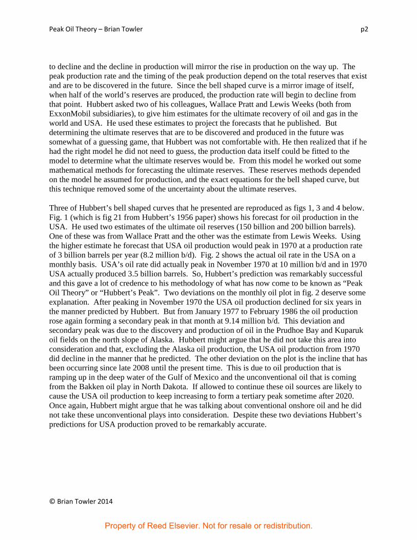
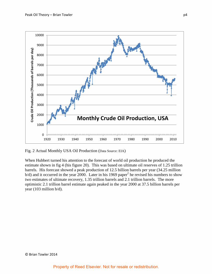
Three of Hubbert’s bell shaped curves that he presented are reproduced as figs 1, 3 and 4 below. Fig. 1 (which is fig 21 from Hubbert’s 1956 paper) shows his forecast for oil production in the USA. He used two estimates of the ultimate oil reserves (150 billion and 200 billion barrels). One of these was from Wallace Pratt and the other was the estimate from Lewis Weeks. Using the higher estimate he forecast that USA oil production would peak in 1970 at a production rate of 3 billion barrels per year (8.2 million b/d). Fig. 2 shows the actual oil rate in the USA on a monthly basis. USA’s oil rate did actually peak in November 1970 at 10 million b/d and in 1970 USA actually produced 3.5 billion barrels. So, Hubbert’s prediction was remarkably successful and this gave a lot of credence to his methodology of what has now come to be known as “Peak Oil Theory” or “Hubbert’s Peak”. Two deviations on the monthly oil plot in fig. 2 deserve some explanation. After peaking in November 1970 the USA oil production declined for six years in the manner predicted by Hubbert. But from January 1977 to February 1986 the oil production rose again forming a secondary peak in that month at 9.14 million b/d. This deviation and secondary peak was due to the discovery and production of oil in the Prudhoe Bay and Kuparuk oil fields on the north slope of Alaska. Hubbert might argue that he did not take this area into consideration and that, excluding the Alaska oil production, the USA oil production from 1970 did decline in the manner that he predicted. The other deviation on the plot is the incline that has been occurring since late 2008 until the present time. This is due to oil production that is ramping up in the deep water of the Gulf of Mexico and the unconventional oil that is coming from the Bakken oil play in North Dakota. If allowed to continue these oil sources are likely to cause the USA oil production to keep increasing to form a tertiary peak sometime after 2020. Once again, Hubbert might argue that he was talking about conventional onshore oil and he did not take these unconventional plays into consideration. Despite these two deviations Hubbert’s predictions for USA production proved to be remarkably accurate.




Fig. 1 Hubbert’s fig 21 shows his 1956 Forecast for USA Oil Production. (Hubbert, 1956)1




Fig. 2 Actual Monthly USA Oil Production (Data Source: EIA)

When Hubbert turned his attention to the forecast of world oil production he produced the estimate shown in fig 4 (his figure 20). This was based on ultimate oil reserves of 1.25 trillion barrels. His forecast showed a peak production of 12.5 billion barrels per year (34.25 million b/d) and it occurred in the year 2000. Later in his 1969 paper2 he revised his numbers to show two estimates of ultimate recovery, 1.35 trillion barrels and 2.1 trillion barrels. The more optimistic 2.1 trillion barrel estimate again peaked in the year 2000 at 37.5 billion barrels per year (103 million b/d).

0

1000

2000

3000

4000

5000

6000

7000

8000

9000

10000

1920 1930 1940 1950 1960 1970 1980 1990 2000 2010

Crud

e O

il Pr

oduc

tion

(Tho

usan

ds o

f bar

rels

per

day

)

Monthly Crude Oil Production, USA




Fig. 3 Hubbert’s 1956 Forecast for World Oil Production. (Hubbert, 1956)1




Fig. 4 Hubbert’s 1969 Forecast of World Oil Production. (Hubbert, 1969)2

It is obvious that the Hubbert forecasts depend on knowing how much oil can be discovered and produced in the world and critics of his method say that this number is only a guess. Can we really know how much oil is going to be eventually discovered and produced in the world? Supporters point out that the timing of the peak is not sensitive to the actual number assumed for the ultimate recovery. Indeed if you examine figs 4 and 5 where three numbers are assumed for the ultimate recovery, ranging from 1.25 trillion to 2.1 trillion barrels, the peak still occurs around the year 2000. Hubbert himself tackled this problem and, borrowing from the mathematics of biological population growth and decay, he devised the mathematical method for forecasting the number for ultimate recovery, which I designate here as Qmax. The equations he used starts with the equation for the cumulative production, Qt, at any time (t). The production rate, qt, at any time t is the derivative of Qt with respect to time, t:

𝑄𝑡 = 𝑄𝑚𝑎𝑥1+𝑎𝑒−𝑏𝑡

(1)

Where

Qt = cumulative production at time, t, usually in barrels

qt = production rate at time, t, usually in barrels/day

Qmax = ultimate cumulative production, usually in barrels

a = growth or decline coefficient, dimensionless




b = growth or decline exponent, dimensions are the reciprocal of time, e.g. 1/days

The production rate, qt at any time (t) is the derivative of the cumulative and so is given by

𝑞𝑡 = 𝑄𝑚𝑎𝑥𝑎𝑏𝑒−𝑏𝑡

�1+𝑎𝑒−𝑏𝑡�2 (2)

Equation 2 is the equation for the production plots shown in figs 1-4. If this model is the correct model for the production data then, as long as we have some early time data, we can fit the data to the model and determine the ultimate recovery, Qmax, as well as the parameters a and b. There are several ways to determine the parameters from the data. The method that Hubbert recommended was to combine equations 1 and 2 to give:

𝑞𝑡 = 𝑏𝑄𝑡 �1 − 𝑄𝑡𝑄𝑚𝑎𝑥

� (3)

Equation 5.3 can then be rearranged to give:

𝑞𝑡𝑄𝑡

= 𝑏 − 𝑏𝑄𝑡𝑄𝑚𝑎𝑥

(4)

Equation 4 then says that if I plot qt/Qt versus Qt then the intercept on the y axis is the parameter b and the intercept on the x axis is the ultimate recoverable oil, Qmax. This plot can be done at any time, even before the peak rate is reached. The timing of the peak can be calculated by taking the derivative of equation 2 and setting it equal to zero. This leads to:

𝑡𝑝𝑒𝑎𝑘 = 1𝑏

ln (𝑎) (5)

But to use equation 5 we need to know the parameter a, which was not determined from the plot of equation 4. The easiest way to determine the parameter, a, is to rearrange equation 1 into the form:

𝑄𝑚𝑎𝑥𝑄𝑡

− 1 = 𝑎𝑒−𝑏𝑡 (6)

Equation 6 says that if I plot the (Qmax/Qt – 1) versus e-bt then the slope of the plot will be equal to a. To do this second plot we assume we have already determined b and Qmax from the plot of equation 5.4. Deffeyes showed his plot of equation 4 using the world production data up until 2005, which is reproduced here as fig. 5. His extrapolation to the x axis shows an intercept of 2 trillion barrels, which is his estimate of the ultimate recoverable oil, Qmax. Note that prior to




1983 the data was increasing and deceasing and had not settled down to form a straight line. But from 1983 to 2005 the data does lie on the straight line that Hubbert’s theory predicts. Deffeyes was also able to deduce his estimate for the time of the peak oil rate directly from his plot, because if the ultimate recovery is projected to be 2 trillion barrels then the peak oil rate will occur when the cumulative production is 1 trillion barrels. This occurred in 2005 and led Deffeyes to predict that oil production would peak in that year.

Fig. 5 Deffeyes Plot of Equation 5.4 for World Oil Production (Deffeyes, Beyond Oil)4

But world oil production did not peak in 2000 or in 2005. Fig 6 shows annual world oil production from 1965 to 2010 and at that time the production was still increasing. Fig 7 shows the world oil production on a monthly basis from the beginning of 1994 to early 2011 and though there are occasional declines the overall trend on both plots is upwards and there is no evidence that a peak has occurred or will occur. The occasional dips in production that have occurred in the past 45 years are due to decreases in demand rather than decreases in supply. However this does not stop the pundits from declaring that world oil production has peaked every time the




production decreases from one year to the next or even from one month to the next. Figs 6 and 7 use data from two different sources. The data for fig 6 come from the BP Annual Statistical Review, while the data for fig. 7 come from the US Energy Information Agency (EIA). So any discrepancies that are perceived between the two plots are due to the different data sources. What is important is that both plots show a consistent upward trend in world oil production. Production did show a secondary peak in 1979 and from 1979 to 1983 production did decrease. This was due to a steep increase in the world oil price in the 1970’s, which resulted in decreased demand in the early 1980’s as people reduced their use of transportation fuels. But from 1983 to the present day there has been a steady increase in oil demand, which has been matched by supply. The world economic crisis that was precipitated in the middle of 2008, tempered demand, causing a decrease in production in late 2008. But from January 2009 to January 2011 there was a persistent increase in production. The uprising in Libya and other countries in the Middle East in early 2011, which is being called the “Arab Spring”, has once again caused a new round of price increases and a resulting decrease in demand for oil but this too is expected to be temporary.

Fig 6 Annual World Oil Production Since 1965 (Data Source: BP Annual Review)

0

10

20

30

40

50

60

70

80

90

1965 1970 1975 1980 1985 1990 1995 2000 2005 2010

Wor

ld O

il Pr

oduc

tion

(Mill

ion

barr

els p

er d

ay) Annual World Oil Production




Fig 7 Monthly World Oil Production Since 1994 (Data Source: EIA)

So what is wrong with the Hubbert model and the analysis of his supporters that has caused their prognostications about the timing of peak oil to be off? I believe that the Hubbert model is essentially correct under a constant price and constant technology scenario. However when the oil price increases, the value of Qmax also increases, as more oil becomes economic to produce. Technology also has an impact. Technology breakthroughs bring more oil reserves into production even under a constant price scenario. Additionally, when the price of oil increases, there is an incentive to develop new technologies, which also increases the oil supply. Price increases and technology breakthroughs seem to unlock large volumes of oil that were previously not economic to produce. In the past twenty years, large reserves in the Canadian oil sands have come on stream. New fracture stimulation and horizontal drilling technologies have also unlocked large reserves of tight oil, tight gas and shale gas. The Canadian oil sands in Alberta have currently booked reserves of 170 billion barrels and the possible reserves reach as high as 1 trillion barrels. Compare that to the slightly more than one trillion barrels of oil that have been produced in the world up until the present time and the one trillion barrels of conventional oil that Deffeyes and Hubbert say are left to be produced. Hundreds of billions of barrels of oil in the Bakken formation in North Dakota, Montana, Manitoba and Saskatchewan are also being unlocked with horizontal wells and multi-zone fracture stimulations. The success in the Bakken is also opening up more formations to successful production, such as the Eagle Ford in Texas, the Granite Wash in Oklahoma and the Texas Panhandle, the Niobrara in

60

65

70

75

80

85

90

1994 1996 1998 2000 2002 2004 2006 2008 2010

Wor

ld O

il Pr

oduc

tion

(mill

ion

barr

els p

er d

ay) Monthly World Oil Production




Colorado and Wyoming, the Monterey in California and the Utica formation in Eastern Ohio. Vast quantities of oil have also been discovered in the deep waters of the Gulf of Mexico and in the Santos offshore basin in Brazil. As these technologies are developed they will be applied to many other areas around the world.

Fig. 8 Average World Price of Crude Oil (Data Source: EIA)

Fig 8 shows the average price of crude oil in the world since 1989 (as determined by the US Energy Information Administration (EIA)). The price increases of 2007-2008 and 2011 have accelerated the deployment of these new technologies as well as the economic development of other marginal reserves. From 1986 to 2005 the price of oil remained relatively constant at around $20/barrel but the warnings from the peak oil theorists in the twenty-first century may have caused the market to start anticipating supply shortages and this, and the political upheavals in the Middle East in 2011, have driven up the price of oil. At the same time they have driven up the value of the world’s ultimate oil reserves, Qmax, and pushed out the timing of the peak production, tpeak. These developments not only affect Qmax and tpeak but will also affect the decline in production on the back side of the Hubbert curve. I will show that we will not be sliding down the other side of the curve in the manner that the Hubbert model forecasts or that the theorists expect. To illustrate this point it is necessary to examine the USA natural gas

$0

$20

$40

$60

$80

$100

$120

$140

1989 1991 1993 1995 1997 1999 2001 2003 2005 2007 2009 2011

Average World Price of Crude Oil ($/barrel)




production curves, which we will look at in the next section of this paper. The history of the US natural gas production has considerable relevance to the trends in world oil supply.

At this point you might also ask why did the Hubbert model work so well in the prediction of the USA oil supply but does not seem to be working, and will not continue to work, for predicting the world oil supply. The answer is simple. The oil market is a world market and the USA oil production peaked and declined amidst a relatively constant world oil price. Even though the USA supply was decreasing, the world supply of oil was stable and the price remained relatively constant from 1986 to 2005. The Hubbert model works as long as the price remains stable. But the world price is now ramping upwards and this will profoundly change the dynamics of the Hubbert model.

For example, if the production data shown in fig. 6 are plotted according to equation 4 we get fig. 9. Extrapolating this to the x-axis gives a value for Qmax of 2.54 trillion barrels, compared with the value of 2 trillion barrels that Deffeyes got using this same data up until 2005. But between 2004 and 2010 the price of oil increased from $20/barrel to $100/barrel and the tight oil in the Bakken and Eagle Ford formations, and the heavy oil sands in Canada and the deepwater oil in the Gulf of Mexico and the Santos Basin became economic to find and produce. In fact another half trillion barrels of oil became economic to produce. If the monthly data published by the EIA, and shown plotted in fig. 7, is used to do the same plot, an even more startling revelation emerges. This plot is shown in fig 10. This is the monthly data from January 1994 to March 2011 and comes from a very reliable source (EIA). When this data is extrapolated to the x-axis the Qmax is 3.055 trillion barrels. Of this 3 trillion barrels 1.3 trillion barrels has already been produced, leaving about 1.7 trillion barrels still to be found and produced. The current listed world oil proved reserves according to EIA is 1.3 trillion barrels, meaning that there are only 400 billion barrels still to be found. But remember that these numbers are a function of oil price and are likely to be conservative. But since this data is probably the most reliable available data, this estimate is probably the most reliable estimate using current economics. It would seem that more oil is appearing all the time. This is due to economics. If and when the price of oil goes up again, and stays up, these numbers will increase again.

The value for the exponential coefficient parameter, a, is obtained using a plot of equation 6. Using this plot and the monthly data from EIA, I obtained a value for a:

a = 162.66

The intercept on the y-axis in fig.10 gave me the value for b:

b = 0.00011733 days-1

Using these values for a and b, I can insert these numbers into equation 5 to calculate the date for the timing of the world peak oil rate.

𝑡𝑝𝑒𝑎𝑘 =1𝑏 ln(𝑎) =

10.00011733 ln(162.66) = 43,396 𝑑𝑎𝑦𝑠




The 43,396 days is measured from an arbitrary time zero, used in the plots, which was 1/1/1900. This equation gives me a peak oil date of October 23, 2018. Note that I am not saying that the world oil production will peak in October 2018. I am saying that using the Hubbert model and the latest and most accurate monthly world oil production data the current projection for the peak oil rate is October 23, 2018. If the price of oil remained constant for the next seven years and there were no big technological breakthroughs during this time this may prove to be an approximately accurate forecast. But I don’t expect that this will be the case and so this date will probably move again.

Fig. 9 Plot of Equation 4 for World Oil Production Data Shown in Fig. 6 (Data Source: BP Annual Review)

0

0.00005

0.0001

0.00015

0.0002

0 0.5 1 1.5 2 2.5 3

q t/Q

t (1/

days

)

Cumulative World Oil Production, Qt (Trillion Barrels)




Fig. 10 Plot of Equation 4 for World Oil Production Data Shown in Fig. 7 (Data Source: EIA)

The USA Gas Supply Analogy to the World Oil Supply

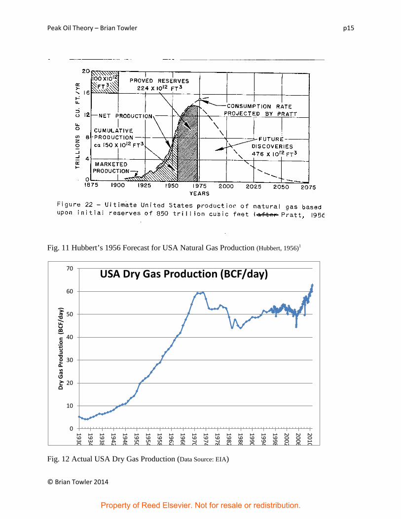
The US gas supply trends have a lot of relevance to the world oil supply behavior. In his 1956 paper1 Hubbert made a forecast of the USA natural gas production, which is reproduced in fig. 11 (his fig 22). This showed the nation’s gas production also peaking in the early 1970’s (around1972) at about 14 trillion cubic feet per year (38 billion cubic feet per day), with an ultimate cumulative production (Qmax) of 850 trillion cubic feet. His figure also showed a line for the projected gas consumption rate which continues to increase after the nation’s gas production peaks and starts to decline. This was a projection using data supplied by Wallace Pratt. Fig. 12 shows the actual USA dry gas production. The units of production rate on this plot are BCF/day. The data shows that the USA peaked in 1973 (almost exactly when Hubbert forecast it) at just below 60 BCF/day. His forecast of the peak year was quite accurate even though his forecast of peak rate was low. The consumption of gas continued to increase as his plot showed and the shortfall that occurred after 1973 was met by imports, mostly by pipeline from Canada.

0

0.00002

0.00004

0.00006

0.00008

0.0001

0.00012

0.00014

0 0.5 1 1.5 2 2.5 3 3.5

q t/Q

t (1/

days

)

Cumulative World Oil Production, Qt (Trillion Barrels)




Fig. 11 Hubbert’s 1956 Forecast for USA Natural Gas Production (Hubbert, 1956)1

Fig. 12 Actual USA Dry Gas Production (Data Source: EIA)

0

10

20

30

40

50

60

70

1930

1934

1938

1942

1946

1950

1954

1958

1962

1966

1970

1974

1978

1982

1986

1990

1994

1998

2002

2006

2010

Dry

Gas

Pro

duct

ion

(BCF

/day

)

USA Dry Gas Production (BCF/day)




In Fig. 12 the production is shown on an annual basis up until 1997 and on a monthly basis from 1997 until the present time (2011). However the decline in production after the peak in 1973 did not happen according to Hubbert’s forecast. The rate began to decline for two years then remained constant for five years. The decline then resumes, finally bottoming out at 44 BCF/day in 1986. Since then there has been a steady increase in production. The production started to increase more sharply in 2006 and today we are making about 63 BCF/day of dry gas. This is more gas than the US was making at the peak in 1973. If the production had declined in a mirror image of the front side of the peak, in 2010 we would expect to see a gas production rate the same as in 1936, when the production was only 6 BCF/day. Instead we are making more than ten times that amount. The Hubbert method has failed miserably to forecast what has happened on the back side of the US gas production curve. The reason for this is economics. Once the nation’s gas supply peaked and a gas shortage developed, the price of gas began to increase. The increased price shook loose gas that was previously uneconomic to produce and the industry began to develop technologies to find and produce coal-bed methane, tight gas and shale gas. This is unconventional gas and it accounts for the majority of the current US gas supply. The US surpassed Hubbert’s estimate of the total ultimate recovery of 850 trillion cubic feet of gas in 1997, and so far have produced more than 1,120 trillion cubic feet without reaching any new peak. Fig 13 shows the gas production repeated with the average annual gas price, which illustrates the effect that price has on the supply. The steep run up in the gas price after the peak has created new supplies of gas, causing the Hubbert model to fail on the back side.

The same thing did not happen to the USA oil supply curve because the oil market is a global market. The price for US oil could not be pushed up in the same way that the gas price was pushed up because the US has always imported a significant portion of its oil and so the US oil producers were constrained to the world price of oil. The world price of oil remained relatively low until recently. However, apart from Canadian supplies and a small and expensive liquefied natural gas (LNG) market, the US gas market is relatively insular.

This analogy illustrates that economics affects the supply of commodities such as oil and gas. In the case of the world oil supply the price of oil has recently been pushed up before the peak of the oil production has been reached. This in turn has pushed out the timing of the peak and indeed the total cumulative production. When the world production of oil does eventually peak (as it must) the back side of the curve will not be a mirror image of the front side of the curve as Hubbert has forecast. It probably will not look like the back side of the US gas supply curve either. It will be controlled by economics and technology, which at this stage are a little difficult to predict.

In his 2010 book “When Oil Peaked”, Ken Deffeyes presents several proofs and analogies to show that the production curves must be symmetrical, that the back side of the curve must be a mirror image of the front side. All of these proofs depend on a constant oil price, which clearly will not happen. If and when oil production does peak the shortage of supply will push the price of oil up and the back side of the curve will not be a mirror image of the front side. The fact that the USA gas production curve is not symmetrical is an indication of the fallacy of Hubbert’s assumption and the subsequent proofs by Deffeyes. I can envisage one scenario where the back side of the world oil production curve might be a mirror image of the front side. At $100/barrel




gas to liquids and coal to liquids technology is economic. If the world began to shift rapidly to these technologies and they are able to maintain their supply at a high enough rate to keep the price of oil constant then the back side of the oil production curve might then be a mirror image of the front side

Fig. 12 USA Dry Gas Production With Average Annual Wellhead Price (Data Source: EIA)

$0

$1

$2

$3

$4

$5

$6

$7

0

10

20

30

40

50

60

70

1930

1934

1938

1942

1946

1950

1954

1958

1962

1966

1970

1974

1978

1982

1986

1990

1994

1998

2002

2006

2010

Aver

age

Annu

al W

ellh

ead

Gas

Pric

e ($

/MM

BTU

)

Dry

Gas

Pro

duct

ion

(BCF

/day

)

USA Dry Gas Production and Wellhead Price




World Oil Reserves

The top twenty countries in the world in terms of proved oil reserves are shown in table 1

Table 1 Crude Oil Proved Reserves (Billion Barrels) (Data Source: EIA)

1 Saudi Arabia 262.6 2 Venezuela 211.2 3 Canada 175.2 4 Iran 137.0 5 Iraq 115.0 6 Kuwait 104.0 7 United Arab Emirates 97.8 8 Russia 60.0 9 Libya 46.4 10 Nigeria 37.2 11 Kazakhstan 30.0 12 Qatar 25.4 13 United States 20.7 14 China 20.4 15 Brazil 12.9 16 Algeria 12.2 17 Mexico 10.4 18 Angola 9.5 19 Azerbaijan 7.0 20 Ecuador 6.5

The number 2 and 3 countries on this list, Venezuela and Canada, owe the majority of their reserves to their heavy oil sands. The total reported proved reserves of crude oil for the entire world is 1.3 trillion barrels, although certain peak oil theorists do not believe that these reserves are correct because they believe that some OPEC members inflate their reserves so that they can get a higher production allocation. I have no reason to believe that these numbers are not approximately accurate and reasonable.

Table 2 Crude Oil Production Rates in 2010 (Thousands of Barrels/day) (Data Source: EIA)

1 Russia 9674 2 Saudi Arabia 8900 3 United States 5474 4 Iran 4080 5 China 4076 6 Canada 2734 7 Mexico 2621 8 Nigeria 2455




9 United Arab Emirates 2415 10 Iraq 2399 11 Kuwait 2300 12 Venezuela 2146 13 Brazil 2055 14 Angola 1939 15 Norway 1869 16 Algeria 1729 17 Libya 1650 18 Kazakhstan 1525 19 United Kingdom 1233 20 Qatar 1127 21 Azerbaijan 1035 22 Indonesia 953 23 Oman 865 24 Colombia 786 25 India 751 26 Argentina 642 27 Malaysia 554 28 Egypt 523 29 Sudan 511 30 Ecuador 486

The world’s top thirty producing countries are listed in table 2. Production rates should have an approximate correlation to reserves, the higher the reserves the higher should be the production rate. In this respect USA does very well. It is producing 5.47 Million b/d from only 20.7 billion barrels of reserves. Countries such as Canada and Venezuela clearly have the capacity to increase their production, although most of their reserves are tied up in very heavy oil, which limits their production rates, because the viscosity of the oil is so low. If Saudi Arabia really has 263 billion barrels of reserves, and I believe that they do, then they could also increase their rates substantially and they have done this at times. But Saudi Arabia has elected to operate as the world’s swing producer, increasing their production when the world demand increases and decreasing production when demand decreases. The Saudis would be happy to increase production if the world demanded it but they are aware that when the price gets too high demand decreases, and the world starts looking for alternatives. USA is producing about the same amount of oil as Saudi Arabia with less than one tenth of their reserves.

There are other countries that also have the capacity to increase their production, and one way to gauge this is to calculate their reserve life, the number of years it would take to produce their reserves if they keep producing at the current rates. Table 3 shows the reserve life of the top thirty countries in this category. Note that the top two countries on this list are once again Venezuela and Canada because of their heavy oil reserves. Any country that has over thirty years of reserve life probably has the potential to increase their production. The USA does not appear in the top thirty on this list because the USA reserve life is only 10.35 years. USA




cannot keep producing oil at its current high rates relative to its reserves unless they are continually drilling new wells and finding more oil. As soon as USA stops drilling its production rate plummets.

Conclusions

The peak in world oil production is dependent on economics and is not likely to occur before 2018. This date will be further extended by rising oil prices and technology developments. When oil rate does eventually peak the back side of the curve will not be a mirror image of the front side of the curve in the manner that Hubbert has predicted. There is still plenty of oil in the world and production will continue to meet demand for some time yet.

References

1. M.K. Hubbert, “Nuclear Energy and the Fossil Fuels”, American Petroleum Institute, Drilling and Production Practices, Proc. Spring Meet., 1956

2. M.K. Hubbert, “Energy Resources”, in National Research Council Committee on Resources and Man, W.H. Freeman, San Francisco, 1969

3. K. S. Deffeyes, “Hubbert’s Peak, The Impending World Oil Shortage”, Princeton University Press, Princeton NJ, 2001

4. K. S. Deffeyes, “Beyond Oil, The View from Hubbert’s Peak”, Hill and Wang, New York NY, 2005

5. K. S. Deffeyes, “When Oil Peaked”, Hill and Wang, New York NY, 2010.




Table 3 Reserve Life (Years) of Oil Producing Countries

1 Venezuela 269.62 2 Canada 175.61 3 Iraq 131.32 4 Kuwait 123.86 5 United Arab Emirates 110.97 6 Iran 91.99 7 Saudi Arabia 80.84 8 Libya 77.08 9 Qatar 61.71 10 Kazakhstan 53.89 11 Netherlands 42.47 12 Nigeria 41.51 13 Ecuador 36.69 14 Chad 32.57 15 Yemen 31.93 16 Bolivia 29.69 17 Sudan 26.79 18 Gabon 24.01 19 Egypt 23.05 20 Brunei 22.13 21 Australia 20.88 22 India 20.72 23 Poland 20.45 24 Trinidad and Tobago 20.31 25 Peru 20.08 26 Malaysia 19.78 27 Algeria 19.34 28 Syria 18.66 29 Romania 18.65 30 Azerbaijan 18.54

More information: The material for this blog was taken from Dr Towler’s new book, “The Future of Energy”, to be published by Elsevier in June 2014.


peak oil theory – brian towler p1 - scitech...

Documents