pedrohenriquethibesforquesato ... · pedrohenriquethibesforquesato...
TRANSCRIPT
Pedro Henrique Thibes Forquesato
Essays in Political and Cultural Economics
Tese de Doutorado
Thesis presented to the Programa de Pós–graduação em Econo-mia of the Departamento de Economia, PUC-Rio, as partial ful-fillment of the requirements for the degree of Doutor em Econo-mia.
Advisor : Prof. Vinicius do Nascimento CarrascoCo-Advisor: Prof. Claudio Abramovay Ferraz do Amaral
Rio de JaneiroApril 2016

Pedro Henrique Thibes Forquesato
Essays in Political and Cultural Economics
Thesis presented to the Programa de Pós–graduação em Econo-mia of the Departamento de Economia, PUC-Rio, as partial ful-fillment of the requirements for the degree of Doutor em Econo-mia. Approved by the following commission:
Prof. Vinicius do Nascimento CarrascoAdvisor
Departamento de Economia – PUC-Rio
Prof. Claudio Abramovay Ferraz do AmaralCo-Advisor
Pontifícia Universidade Católica do Rio de Janeiro – PUC-Rio
Prof. Leonardo Bandeira RezendeDepartamento de Economia - PUC-Rio – PUC-Rio
Prof. Juliano Junqueira AssunçãoDepartamento de Economia - PUC-Rio – PUC-Rio
Prof. João Manoel Pinho de MelloINSPER – INSPER
Prof. César Zucco JuniorEscola Brasileira de Administração Publica e de Empresas -
FGV – EBAPE/FGV
Prof. Monica HerzCoordenador Setorial do Centro de Ciências Sociais – PUC-Rio
Rio de Janeiro, April 1st, 2016
All rights reserved.
Pedro Henrique Thibes Forquesato
Pedro Forquesato holds a B.A. in Economics from the Uni-versidade Estadual de Campinas (Unicamp) and a Ph.D. inEconomics from the Catholic University of Rio de Janeiro(PUC-Rio). During his Ph.D. studies, he was visiting scholarat the John F. Kennedy School of Government at HarvardUniversity for a period of one year. His research focus onpolitical and cultural aspects of development and economictheory.
Ficha CatalográficaForquesato, Pedro
Essays in Political and Cultural Economics / Pedro Hen-rique Thibes Forquesato; advisor: Vinicius do Nascimento Car-rasco; co-advisor : Claudio Abramovay Ferraz do Amaral. –2016.
v., 90 f: il. ; 30 cm
1. Tese (doutorado) - Pontifícia Universidade Católica doRio de Janeiro, Departamento de Economia, 2016.
Inclui bibliografia.
1. Economia – Tese. 2. Economia Política. 3. EconomiaCultural. 4. Redistribuição de Renda. 5. Risco Moral. 6. Éticado Trabalho. I. Carrasco, Vinicius. II. Ferraz, Claudio. III. Pon-tifícia Universidade Católica do Rio de Janeiro. Departamentode Economia. IV. Título.
CDD: 330
Acknowledgments
First and foremost, I would like to thank my wife, Xinxin Jiang, for thelove and company. I would also want to thank my family, especially my parents,Mônica and Edson, and my siblings Camila and Luís.
I am deeply grateful to my advisor, Vinicius Carrasco, for his vitalsupport in all stages of the production of this thesis, support which far exceededhis formal obligation as advisor. I am also thankful to my co-advisor ClaudioFerraz, with whom I wrote the third chapter of this thesis, but who also had acrucial role in the development of the first two. I am indebted to all membersof the committee. João Manoel, Leo, Juliano and César, all had significantcomments and suggestions before and during the thesis defense; they improvedthis thesis significantly and also helped shape me as a researcher.
I am grateful to all my professors, during undergraduate and graduatestudies, which gave me a solid basis in economics that allowed me to developthe research that led to this thesis. There is something of each of them in whatis best in these articles. (Possible shortcomings are entirely my fault.) I am alsograteful to the employees of the Departamento de Economia of PUC-Rio fortheir indispensable support during the five years I stayed in this institution.
I am particularly indebted to Professor Filipe Campante of HarvardUniversity, for having received me during my period as visiting scholar in thatinstitution, and having actively participated in my formation as a researcher,as well as helping develop the research that would eventually become thisthesis. I thank all professors and students of Harvard University, for havingso kindly embraced me when I was alone in a foreign and unknown country,being always willing to discuss research and help me develop as an academic.
This thesis would have not been possible without the companionshipof my graduate colleagues, as well as all my other friends in PUC-Rio andCampinas which stood by my side and wished for my success in the moredifficult moments in these five years of intense study and research.
Finally, I am grateful to the financial support of CAPES, both duringmy PhD in Brazil as well as during my research period in United States, andCNPq.
Abstract
Forquesato, Pedro; Carrasco, Vinicius; Ferraz, Claudio. Essays inPolitical and Cultural Economics. Rio de Janeiro, 2016. 90p.PhD Thesis – Departmento de Economia, Pontifícia UniversidadeCatólica do Rio de Janeiro.
This thesis is composed of three papers, the first in organizationaleconomics and culture; the last two in political economics. In the first chap-ter, we model the relation between dissemination of social norms of workethic and incentives proposed by firms, which we motivate using evidencefrom three different datasets. In the second chapter, we examine whetherneighbors’ income affects voting, using data from election results for the2004-2012 Presidential Elections in Unites States, by precinct and blockgroup. That way, we try to contribute to understanding the reason whythere are different demands for income redistribution. As an identificationstrategy, we use year fixed-effects and tract year dummies; tract is the small-est geographic unit larger than block group (on average, each tract contains4 block groups). In the third chapter, we study patronage, investigating theeffect of a mayoral candidate’s victory on the probability that members ofhis party (or parties in the same presidential coalition) occupy public jobs inthe government, or on their income accrued from government, in case theyare already public employees. We also analyze the effect of a party’s vic-tory over the number of registered members of that party in future years,which would indicate that voters affiliate to political parties as a way tosignal support to the office holder. We estimate plausibly causal effects ofa party holding mayoral position by comparing municipalities where thatparty nearly won with places where it nearly lost.
KeywordsPolitical Economics. Cultural Economics. Income Redistribution.
Moral Hazard. Work Ethic.
Resumo
Forquesato, Pedro; Carrasco, Vinicius; Ferraz, Claudio. Ensaiosem Economia Política e Cultura. Rio de Janeiro, 2016. 90p.Tese de Doutorado – Departamento de Economia, Pontifícia Uni-versidade Católica do Rio de Janeiro.
Esta tese é formada por três artigos, o primeiro em economiaorganizacional e cultura; os dois últimos em economia política. No primeirocapítulo, nós modelamos a relação entre a disseminação de normas sociaisde ética do trabalho e incentivos propostos pelas firmas, que motivamosutilizando evidência de três bases de dados diferentes. No segundo capítulo,examinamos se a renda dos vizinhos afeta o voto de eleitores, utilizandodados de resultados de eleições presidenciais (2004 até 2012) nos EstadosUnidos, por zona eleitoral e grupo de bairros. Com isso, buscamos contribuirpara o entendimento das razões que levam a diferentes níveis de demandapor redistribuição de renda. Como estratégia de identificação, utilizamosefeitos fixos de ano e dummies de trato e ano; trato sendo a menor unidadegeográfica maior que o grupo de blocos (em média, um trato contém 4 gruposde blocos). No terceiro capítulo, estudamos patronagem, investigando oefeito da vitória de um candidato a prefeito de um partido na probabilidadede membros deste partido (ou de partidos da mesma coalizão) ocuparemcargos públicos no governo; ou de sua renda advinda do governo aumentar,caso já sejam empregados públicos. Analisamos também o efeito da vitóriade um partido sobre o número de registrados a este partido nos anosfuturos, o que indicaria um desejo de sinalizar apoio ao candidato eleito.Estimamos o efeito causal de um partido ocupar a prefeitura, comparandomunicipalidades em que este partido quase ganhou com cidades em quequase perdeu.
Palavras-chaveEconomia Política. Economia Cultural. Redistribuição de Renda.
Risco Moral. Ética do Trabalho.
Sumário
1 Social Norms of Work Ethic and Incentives in Organizations 111.1 Introduction 111.2 Work Ethic 151.3 Basic Facts 161.3.1 International Social Survey Programme 171.3.2 European Social Survey and European Values Study 201.3.3 World Values Survey and Execucomp 231.4 Model 251.4.1 Moral Hazard in Teams Game 251.4.2 Cultural Transmission Process 281.5 Discussion 321.6 Extensions 341.6.1 Firm Selection 351.6.2 Comparative Dynamics 381.7 Conclusion 40
2 Neighbors’ Income and Demand for Redistribution 422.1 Introduction 422.2 Data 452.3 Empirical Strategy 462.4 Results 492.5 Discussion 522.6 Conclusion 56
3 Party Registration and Mayoral Elections 583.1 Introduction 583.2 Data 603.3 Party Affiliation in Brazil 623.4 Empirical Strategy 673.5 Results 683.5.1 Government Wages 693.5.2 Party Registration 713.6 Conclusion 75
Referências Bibliográficas 78
A Proofs of propositions of Chapter 1 83A.1 Proof of Proposition 1.1 83A.2 Proof of Proposition 1.2 84A.3 Proof of Proposition 1.3 85A.4 Proof of Proposition 1.4 88
B Further specifications for Chapter 2 89
Lista de figuras
1.1 Cross-country correlations between work ethic and effort at work(ISSP 1989, 1997). 17
1.2 Cross-country correlation between work ethic and incentive steep-ness (EVS 2008, ESS 2004, 2010) 21
1.3 Dynamics of work ethic for an example parameter profile. (α = 0.7,θ = 0.25, ρ = 10, κN = 0.8, κW = 0.4, KW = 0.6) 31
1.4 Dynamic system of xW and βC for an example parameter profile.(θ = 0.25, ρ = 10, α = 0.7, κW = 0.4, κN = 0.8, γ = 0.55,ζ = 0.8, and KW = 0.45) 36
1.5 Dynamic system of xW and βC (θ = 0.25, ρ = 10, α = 0.7,κW = 0.4, κN = 0.8, γ = 0.55, ζ = 0.8, and KW = 0.4) 39
2.1 Votes for Democrats (blue) as opposed to Republicans (red) for2008 Presidential Election (Ohio). 46
2.2 Moran graph for share of votes for Democrats (Moran’s I: 0.59,p-value 0.00). 49
3.1 Party affiliates by party and election year (9 largest parties in 2012). 633.2 Party registrations for parties in presidential and opposition coaliti-
ons, per year. 643.3 Party registrations for parties in presidential and opposition coaliti-
ons, monthly (2008). 653.4 Estimated density function around the cutoff (McCrary test). 693.5 Effect of mayoral victory on wages accrued from government, for
individuals registered to parties in the presidential coalition. 703.6 Effect of mayoral victory on percent working for the government,
for individuals registered to parties in the presidential coalition. 703.7 Effect of mayoral victory on future party affiliations, for individuals
registered to parties in the presidential coalition. 75
Lista de tabelas
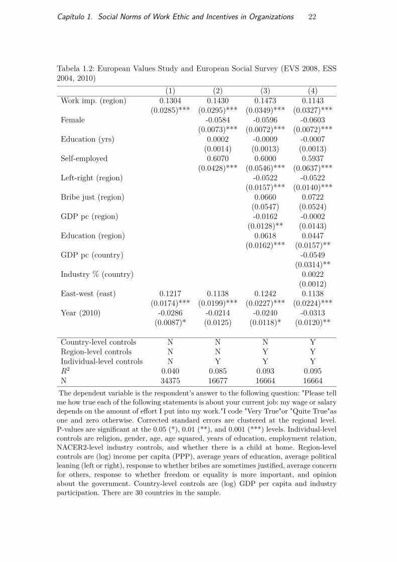
1.1 Correlation between work ethic and effort at work (ISSP 1989, 1997) 191.2 European Values Study and European Social Survey (EVS 2008,
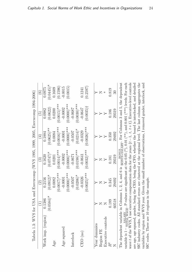
ESS 2004, 2010) 221.3 WVS for USA and Execucomp (WVS 1995, 1999, 2005, Execucomp
1994-2006) 24
2.1 Descriptive Statistics. 482.2 Neighbors’ Income and Votes for Democrats (Ohio, 2004-08). 502.3 Neighbors’ Income and Votes for Democrats (Ohio, 2004-08),
spatial models. 512.4 Neighbors’ Income and Votes for Democrats (Ohio, 2004-08), per
party and US House of Representatives. 532.5 Neighbors’ Income and House Values (Ohio, 2004-08). 55
3.1 Summary statistics (full sample), separated by treatment and con-trol (registered to a member of presidential coalition, where itwon—resp. lost—the election). 62
3.2 Summary statistics (full sample, aggregated by party-city), separa-ted by treatment and control. 63
3.3 Summary statistics (before and after registration deadline to runfor 2008 elections). 66
3.4 Summary statistics (full RAIS and affiliated). 663.5 Balance test. Treatment (resp. control) is registered to a member
of presidential coalition, where it won (resp. lost) the election. 683.6 Effect of party victory in mayoral elections on probability of registe-
red individuals working for government, and income from government. 723.7 Effect of party victory in mayoral elections on probability of regis-
tered individuals working for government, and income from govern-ment (political parties). 73
3.8 Effect of party victory in mayoral elections on probability of regis-tered individuals working for government, and income from govern-ment (pooled). 74
3.9 Effect of party victory in mayoral elections on future party registra-tions. 76
B.1 Neighbors’ Income and Votes for Democrats (United States, 2004-2012). 90
Because of the success of science, there is akind of a pseudo-science. Social science is anexample of a science which is not a science.They follow the forms. You gather data, youdo so and so and so forth, but they don’t getany laws, they haven’t found out anything.They haven’t got anywhere – yet. Maybe so-meday they will, but it’s not very well develo-ped...See, I have the advantage of having found outhow hard it is to get to really know something,how careful you have to be about checking yourexperiments, how easy it is to make mistakesand fool yourself. I know what it means toknow something. And therefore, I see how theyget their information. And I can’t believe thatthey know when they haven’t done the worknecessary, they haven’t done the checks neces-sary, they haven’t done the care necessary.
Richard Feynman, Interview to BBC, 1981.
1Social Norms of Work Ethic and Incentives in Organizations
"Seest thou a man diligent in his business? He shall stand beforekings."(Proverbs, 22-29.)
1.1Introduction
For a long time, sociologists and classical economists have defendedthe importance of cultural values of work effort (henceforth, work ethic) inexplaining differences in development ((03)), and a recent body of literature((15), (16)) uses historical evidence to emphasize the importance of theseexplanations. That literature, however, does not clearly grasp how thesedifferences in cultural values emerge and spread in different societies.1
In this paper, I hypothesize that differences in the dissemination of workethic emerge endogenously from multiple equilibria in cultural transmissiondecisions made by parents and incentive choices made by firms. I build a modelthat shows how this process would occur, and I substantiate it using anecdotaland empirical evidence that firm incentives are an important determinant of(intergenerational) cultural transmission.
In my model, parents altruistically choose whether to transmit work ethicto their offspring, taking into account the effect it will have on their utility.Where incentives are high-powered (that is, where payment is more dependenton success), parents expect that their children will work harder, and workethic will be more rewarding for them. In these societies, parents have strongerincentives to transmit work ethic, and work ethic slowly disseminates. Incentivesteepness (as in how high-powered the incentives are) has an effect on workethic.
When there is complementarity of effort between workers, having anemployee with a strong work ethic (who, in equilibrium, will exert highereffort) improves the productivity of his peers. Having more productive workers,the firm optimally chooses to offer high-powered incentives in order to take
1The literature is not unanimous, for example, on Weber’s own explanation for theemergence of these cultural norms. See (20) and (19). I discuss how my explanation relatesto Weber’s in Section 5.

Capítulo 1. Social Norms of Work Ethic and Incentives in Organizations 12
advantage of the higher productivity of its employees by inducing them towork harder. If worker effort is complementary, then in societies in which theproportion of individuals with work ethic is higher, firms choose to offer steeperincentives and demand more effort.
Consequently, the model has two equilibria. When a large proportion ofthe society’s workforce has a strong work ethic, firms offer steeper incentiveseven to employees without a work ethic, as having high-effort coworkers makesthem more productive. If firms choose high-powered incentives, then agentswork hard and cultural values that stimulate effort are particularly useful tothem. If a small proportion of the workforce has a work ethic, then workersshirk more, making their coworkers less productive and causing firms to chooseless high-powered incentives and demand less effort, even from workers witha strong work ethic. As individuals work less, work ethic is less useful, andparents have weaker incentives to transmit it.
Having established the main argument, I augment the benchmark modelby allowing firms to choose their production technologies, adopting either acomplementary technology in which an agent’s productivity is highly depen-dent on his coworkers’ or a separable technology in which interdependenciesamong workers are minimal. I interpret this choice as one between modernproduction processes, such as Fordism or lean manufacturing—more efficientways of organizing production in which a worker’s productivity is highly de-pendent on his peers’ effort—and traditional technologies, such as the putting-out system, which is less efficient overall but creates less dependency betweencoworkers.2
This extended model also has two equilibria, one in which firms usetraditional technologies and workers do not have a strong work ethic andanother in which firms adopt modern production processes and a strong workethic is disseminated throughout the society. This pattern matches stylizedhistorical facts and helps explain why countries in which labor is unproductiveare reluctant to adopt new technologies and organizational structures fromdeveloped countries. A similar argument is made in (22). Here, I contribute byexplicitly modeling the worker’s effort and the firm’s incentive choice. Thus, mymodel also clarifies why managers do not employ different incentive schemes infirms whose labor productivity is low and explains the evidence provided in (15)
2Fordism is a system of mass production pioneered in the early 20th century by theFord Motor Company based, inter alia, on the use of assembly lines. Lean manufacturingis a management philosophy derived mostly from the Toyota Production System, whichfocuses on reducing waste by having the "right tools in the right place at the right time."Atthe opposite end of the spectrum from these very complex and complementary processes isthe putting-out system wherein a central agent subcontracts production to off-site facilities(usually the worker’s own home).
Capítulo 1. Social Norms of Work Ethic and Incentives in Organizations 13
that effort, even more than skill, differentiates regions in terms of productivity.To show the importance of the relation between incentive steepness
and work ethic beyond the use of historical examples, I examine 3 differentdatasets and show that wider dissemination of work ethic is correlated withmeasures of incentive steepness and effort at work. First, using data fromthe International Social Survey Programme, I show that people are morelikely to arrive from home exhausted, a measure of effort, when living incountries in which the proportion of people who believe that work is a person’smost important activity is high. I then use data from the European ValuesStudy and the European Social Survey to show that in regions in which morepeople believe that hard work is an important characteristic that should betaught at home, wages are more likely to depend on effort, a measure ofincentive steepness. Finally, I go beyond self-reported measures by examiningthe correlation between work ethic and executive compensation, using actualdata from Standard & Poor’s Execucomp for the United States. The resultsof these empirical exercises are consistent with the model: workers in areaswith wider dissemination of work ethic are more likely to receive high-poweredincentives and to work harder, on average, indicating the importance of culturalnorms to understanding the behaviors of workers and firms.
This paper is embedded in a new and growing literature on the intergene-rational transmission of cultural traits, which is reviewed in (13). In particular,in my model, parents are imperfectly altruistic when choosing how to socia-lize their offspring, as in (01, 02). My cultural transmission process, however,includes endogenous cultural intolerance (that is, the benefit of socializing anindividual to value a trait depends on its dissemination throughout the societyrather than on exogenous factors), which is determined by the average incen-tive scheme chosen by firms. This scheme is a function of the proportion ofagents with a strong work ethic in the society. In fact, as parents will wantto instill a strong work ethic when most individuals have it, the model exhi-bits strategic complementarity in the socialization process (as in, for example,(17)).3
Closely related to work ethic, a growing literature investigates culturalbeliefs about the returns to effort, although its focus has been on explainingredistribution choices and social protection (as in (05) and (04)). While thesepapers provide an important mechanism by which differences in effort andcultural norms of work exist among countries, namely, the political choices ofsocial insurance and redistribution, they are less able to explain why thesedifferences might exist within countries (as between southern and northern
3See (13) for other references with endogenous cultural intolerance.
Capítulo 1. Social Norms of Work Ethic and Incentives in Organizations 14
Italy), where redistribution levels are roughly similar, or in non-democraticsocieties, where redistribution levels are not decided by majority voting.
Furthermore, my model yields various policy implications. If multipleequilibria emerge as a consequence of different levels of redistribution andbeliefs about returns to effort, then an exogenous change in taxes and transferswould cause a change of equilibrium. In my model, however, that is notnecessarily true. A reduction in taxes in a region with a poorly disseminatedwork ethic might not be sufficient to change the equilibrium, as it mightstill be optimal for parents to not instill their offspring with work ethicbecause firms employ low-powered incentives. In this sense, I contribute tothe literature by offering an alternative (and complementary) mechanism thatcan explain differences in effort and does not depend on political mechanisms.Moreover, the fact that the empirical evidence shows that incentive steepness iscorrelated with measures of work ethic suggests that my mechanism is relevantto explaining differences in work behavior across regions.
Perhaps the closest paper to ours is (21). They develop a model inwhich the middle class chooses to transmit a work ethic while the nobilityprefers to transmit preferences for leisure. With the Industrial Revolution, awork ethic becomes particularly advantageous, and the middle class takes overand becomes the new entrepreneurs and the dominant economic class. Themain difference between their model and mine is that I endogenize the choiceof incentives made by firms and focus my analysis on effort exertion ratherthan on labor supply. This specification is important both in order to explainthe anecdotal evidence that worker effort is an important determinant ofproductivity and to explain the empirical evidence that work ethic is correlatedwith incentive steepness, a facet that can only be meaningfully analyzed inagency models.4
The rest of this paper is organized as follows. In Section 3, I presentempirical evidence that suggests that worker effort and incentive steepness varyby region and that this variation is robustly correlated to regional differencesin work ethic. In Section 4, I present a model of intergenerational transmissionof work ethic and incentives in organizations, and I argue that the modelcan explain a set of stylized facts. In Section 5, I discuss some assumptionsand results of the model, while in Section 6, I extend it by consideringthe implications of firms being able to choose whether their technology ischaracterized by complementarity. I analyze the comparative dynamics of this
4Also related are the literatures on the evolutionary selection of human traits ((62), (63))and on contracting with social norms ((09), (08), (06), (11), (64), (32), (12) (61), and (60)).Other approaches to studying norms of hard work include (10) and (18).

Capítulo 1. Social Norms of Work Ethic and Incentives in Organizations 15
extended model. Finally, I conclude with a discussion of my results and avenuesfor future research.
1.2Work Ethic
Since the 19th Century, classical economists and sociologists have ob-served that regions exhibit very different cultural norms of hard work andaffirmed that this difference is a major cause of productivity (and, consequen-tly, of income) inequality between societies. Max Weber, for example, in hisbook about the Protestant work ethic, wrote:
"As every employer knows, the lack of coscienziositá [diligence]of the labourers of such countries, for instance Italy as comparedwith Germany, has been, and to a certain extent still is, one ofthe principal obstacles to their capitalistic development. Capitalismcannot make use of the labour of those who practice the doctrineof undisciplined liberum arbitrium [free will] ...."(03, p. 21).
Summarizing the importance of work ethic for economic (capitalistic)development, Weber writes, "This peculiar idea (...) of one’s duty in a calling,is what is most characteristic of the social ethic of capitalistic culture"(03,p. 19).
Here, work ethic is understood as a cultural norm that is internalizedby agents and makes shirking costlier while providing moral support for higheffort, reducing its cost. Examples of this thought abound in historical andreligious sources. Benjamin Franklin, for example, in his "Advice to a YoungTradesman, Written by an Old One,"writes:
"The Sound of your Hammer at Five in the Morning or Nineat Night, heard by a Creditor, makes him easy Six Months longer.But if he sees you at a Billiard Table, or hears your Voice in aTavern, when you should be at Work, he sends for his Money thenext Day."(30).
Another important source of social norms of effort is religion. As Baxterstates, "It is for action that God maintaineth us and our activities; work is themoral as well as the natural end of power."(31, p. 375). Moreover, work ethicis not only a social norm that values effort and dedication but also one thatcondemns leisure and shirking. Baxter (as cited by Weber) dictates, "Wasteof time is thus the first and in principle the deadliest of sins. (...) Loss oftime through sociability, idle talk, luxury, (...) is worthy of absolute moralcondemnation."(03, p. 104).

Capítulo 1. Social Norms of Work Ethic and Incentives in Organizations 16
Therefore, while a strong work ethic is useful in a utilitarian sense for hardworking individuals, promising ethical, monetary, or religious compensation fortheir toil, it is detrimental to individuals who favor leisure, as it imposes guiltfor and moral condemnation of their low effort.
1.3Basic Facts
Recent empirical evidence substantiates Weber’s claim that there aresizable differences in work norms and effort among societies. (07), whileinvestigating the behavior of the employees of a large Italian bank, discoverthat those working in branches in southern Italy were significantly more likelyto shirk then employees of northern Italian branches. Moreover, individualpreferences for shirking and work explain most of this differential (rather thansorting, peer effects, or firm attributes). Gregory Clark provides anecdotalevidence that also points to significant differences in worker behavior acrossregions:5
"In fact workers in poorly performing economies simply supplyvery little actual labor input on the job. Workers in modern cottontextile factories in India, for example, are actually working for aslittle as fifteen minutes of each hour they are at the workplace."(15,p. 13).
Furthermore, he argues that this low level of effort in factories waswell known by managers and firm owners, which raises the question of whymanagers did not incentivize their employees to work harder.6 By endogenizingthe choice of incentives (and hence, indirectly, work effort), my model canprovide an answer to this puzzle.7
In the rest of this section, I present quantitative evidence from threedifferent datasets that is consistent with work ethic variation among regionsand is correlated with both effort provision and incentive steepness. I providedescriptive statistics and some alternative specifications in Appendix B.
5For related arguments, see also (16).6(15) mentions, for example, that "[t]o partially control this absenteeism some employers
used a pass system, under which a worker could leave the mill only with a pass or tokenfrom his or her department. Each department was allotted passes equal to 10-25 percent ofthe staff."
7Another possible explanation for this puzzle is collusion between managers and workers.Clark offers evidence that this mechanism was not very important. For example, in 1895,in Bombay, of 55 mill managers, 27 were British, as were 77 of the 190 weaving mastersand other managerial positions. It seems implausible that British managers would be morewilling to collude with Indian workers than with British ones.
Capítulo 1. Social Norms of Work Ethic and Incentives in Organizations 17
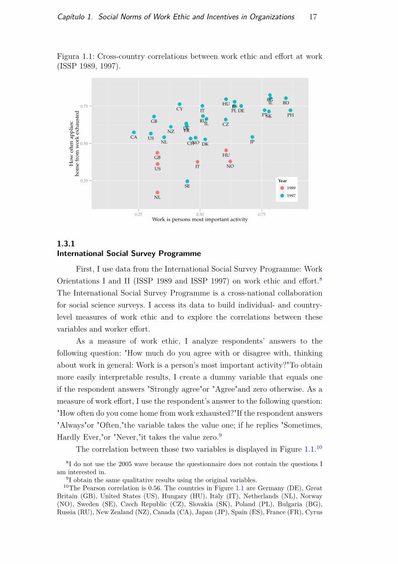
Figura 1.1: Cross-country correlations between work ethic and effort at work(ISSP 1989, 1997).
BGBD
CACH
CY
CZ
DE
DK
DE
ES
FR
GB
GB
HU
HU
IT
IT
IL
IL
JP
NO
NO
NL
NL
NZ
PTPL
PHRU
SE
SK
US
US
0.25
0.50
0.75
0.25 0.50 0.75Work is persons most important activity
How
ofte
nap
plie
s:ho
me
from
wor
kex
haus
ted
Year
1989
1997
1.3.1International Social Survey Programme
First, I use data from the International Social Survey Programme: WorkOrientations I and II (ISSP 1989 and ISSP 1997) on work ethic and effort.8
The International Social Survey Programme is a cross-national collaborationfor social science surveys. I access its data to build individual- and country-level measures of work ethic and to explore the correlations between thesevariables and worker effort.
As a measure of work ethic, I analyze respondents’ answers to thefollowing question: "How much do you agree with or disagree with, thinkingabout work in general: Work is a person’s most important activity?"To obtainmore easily interpretable results, I create a dummy variable that equals oneif the respondent answers "Strongly agree"or "Agree"and zero otherwise. As ameasure of work effort, I use the respondent’s answer to the following question:"How often do you come home from work exhausted?"If the respondent answers"Always"or "Often,"the variable takes the value one; if he replies "Sometimes,Hardly Ever,"or "Never,"it takes the value zero.9
The correlation between those two variables is displayed in Figure 1.1.10
8I do not use the 2005 wave because the questionnaire does not contain the questions Iam interested in.
9I obtain the same qualitative results using the original variables.10The Pearson correlation is 0.56. The countries in Figure 1.1 are Germany (DE), Great
Britain (GB), United States (US), Hungary (HU), Italy (IT), Netherlands (NL), Norway(NO), Sweden (SE), Czech Republic (CZ), Slovakia (SK), Poland (PL), Bulgaria (BG),Russia (RU), New Zealand (NZ), Canada (CA), Japan (JP), Spain (ES), France (FR), Cyrus
Capítulo 1. Social Norms of Work Ethic and Incentives in Organizations 18
It shows that both work ethic and effort differ significantly by country in bothyears, although work ethic seems to vary little from 1989 to 1997 in countrieswith both values, which is consistent with the view of culture as slow to change.Moreover, there is a correlation between how important people in a countryconsider work and how much effort, on average, people exert at work. Thiscorrelation seems to hold for both years for which there is data. I provide moreevidence on this below.
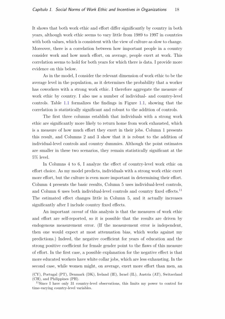
As in the model, I consider the relevant dimension of work ethic to be theaverage level in the population, as it determines the probability that a workerhas coworkers with a strong work ethic. I therefore aggregate the measure ofwork ethic by country. I also use a number of individual- and country-levelcontrols. Table 1.1 formalizes the findings in Figure 1.1, showing that thecorrelation is statistically significant and robust to the addition of controls.
The first three columns establish that individuals with a strong workethic are significantly more likely to return home from work exhausted, whichis a measure of how much effort they exert in their jobs. Column 1 presentsthis result, and Columns 2 and 3 show that it is robust to the addition ofindividual-level controls and country dummies. Although the point estimatesare smaller in these two scenarios, they remain statistically significant at the5% level.
In Columns 4 to 6, I analyze the effect of country-level work ethic oneffort choice. As my model predicts, individuals with a strong work ethic exertmore effort, but the culture is even more important in determining their effort.Column 4 presents the basic results, Column 5 uses individual-level controls,and Column 6 uses both individual-level controls and country fixed effects.11
The estimated effect changes little in Column 5, and it actually increasessignificantly after I include country fixed effects.
An important caveat of this analysis is that the measures of work ethicand effort are self-reported, so it is possible that the results are driven byendogenous measurement error. (If the measurement error is independent,then one would expect at most attenuation bias, which works against mypredictions.) Indeed, the negative coefficient for years of education and thestrong positive coefficient for female gender point to the flaws of this measureof effort. In the first case, a possible explanation for the negative effect is thatmore educated workers have white collar jobs, which are less exhausting. In thesecond case, while women might, on average, exert more effort than men, an
(CY), Portugal (PT), Denmark (DK), Ireland (IE), Israel (IL), Austria (AT), Switzerland(CH), and Philippines (PH).
11Since I have only 31 country-level observations, this limits my power to control fortime-varying country-level variables.
Capítulo 1. Social Norms of Work Ethic and Incentives in Organizations 19
Tabe
la1.1:
Correlatio
nbe
tweenwo
rkethican
deff
ortat
work
(ISS
P19
89,1
997)
(1)
(2)
(3)
(4)
(5)
(6)
Workim
portan
t0.0883
0.04
320.01
670.05
220.01
630.0128
(0.011
8)**
*(0.012
6)**
*(0.007
1)*
(0.0068)**
*(0.006
2)**
(0.006
2)*
Workim
p.(cou
ntry)
0.34
800.30
670.57
39(0.086
1)**
*(0.106
8)**
(0.060
0)**
*Ed
ucation(yrs)
-0.013
8-0.011
0-0.010
7-0.011
0(0.003
0)**
*(0.002
4)**
*(0.002
8)**
*(0.0024)**
*Fe
male
0.1047
0.10
850.10
750.10
91(0.008
8)**
*(0.008
3)**
*(0.008
1)**
*(0.0082)**
*Ye
ar(199
7)0.27
620.26
280.25
300.25
780.2247
0.24
69(0.029
0)**
*(0.035
7)**
*(0.0478)**
*(0.028
1)**
*(0.038
8)**
*(0.029
5)**
*
Individu
al-le
velc
ontrols
NY
YN
YY
Cou
ntry
dummies
NN
YN
NY
R2
0.05
80.12
40.16
30.06
90.13
20.17
0N
4061
732
018
3201
840
617
3201
832
018
The
depe
ndentvaria
bleis
therespon
dent’s
answ
erto
"How
oftendo
youcomeho
mefrom
workexha
usted?
"Icode
"Always"or
"Often
"ason
e"Som
etim
es,H
ardlyEv
er,"o
r"N
ever"aszero.C
orrected
stan
dard
errors
areclusteredat
the
coun
trylevel.P-
values
aresig
nific
antat
the0.05
(*),
0.01
(**),a
nd0.001(***)levels.
Individu
al-le
velc
ontrolsare
yearsof
educ
ation,
sex,
age,
agesqua
red,
andself-repo
rted
social
class.
The
reare31
coun
try-levelo
bservatio
ns.
Capítulo 1. Social Norms of Work Ethic and Incentives in Organizations 20
alternative explanation would be that they are more easily exhausted, and it isimpossible to distinguish between these conjectures. Notwithstanding, as longas people with a strong work ethic are not more prone to feeling exhausted(or reporting that they feel exhausted) than those without, my measures willunderestimate the total importance of work ethic on effort.
1.3.2European Social Survey and European Values Study
My second empirical exercise uses data from the European Social Survey:Family, Work and Well Being (ESS2 2004 and ESS5 2010) and the 4th Waveof the European Values Study (EVS 2008) to form a database of measuresof work ethic at the regional level and work attitudes at the individual level.The advantage of this database is that the ESS includes questions that areplausible indicators of the steepness of incentives. (The interest is in how high-powered the incentives are, not in how high the wages are, which is more easilymeasurable.)
From the EVS 2008, I aggregate an indicator of work values at theregional level, namely, if the respondent mentioned "hard work"when askedthe following question: "Here is a list of qualities which children can beencouraged to learn at home. Which, if any, do you consider to be especiallyimportant? Please choose up to five."I argue that this variable best captures theintergenerational aspect of the cultural transmission of work ethic; nonetheless,my result is robust to the use of other related questions.
I use the ESS data to obtain individual, self-reported measures of thesteepness of incentives. I use respondents’ answers to the following question:"Please tell me how true each of the following statements is about your currentjob: my wage or salary depends on the amount of effort I put into my work."Tosimplify interpretation, again I code the responses as dummy variables.
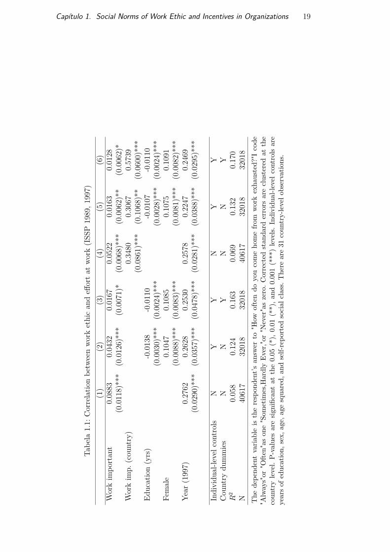
Figure 1.2 shows the correlation between self-reported incentive steepnessand country-level work ethic for European countries in 2004 and 2010.12 Thecorrelation is strong (0.63); the probability that the respondent considers hiswage highly dependent on effort in countries with high work ethic is twice aslarge as that in countries with low work ethic.
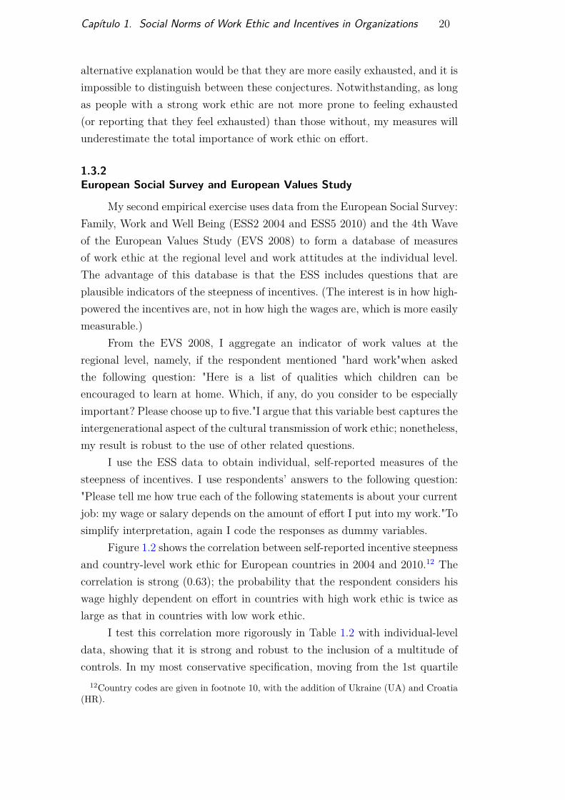
I test this correlation more rigorously in Table 1.2 with individual-leveldata, showing that it is strong and robust to the inclusion of a multitude ofcontrols. In my most conservative specification, moving from the 1st quartile
12Country codes are given in footnote 10, with the addition of Ukraine (UA) and Croatia(HR).
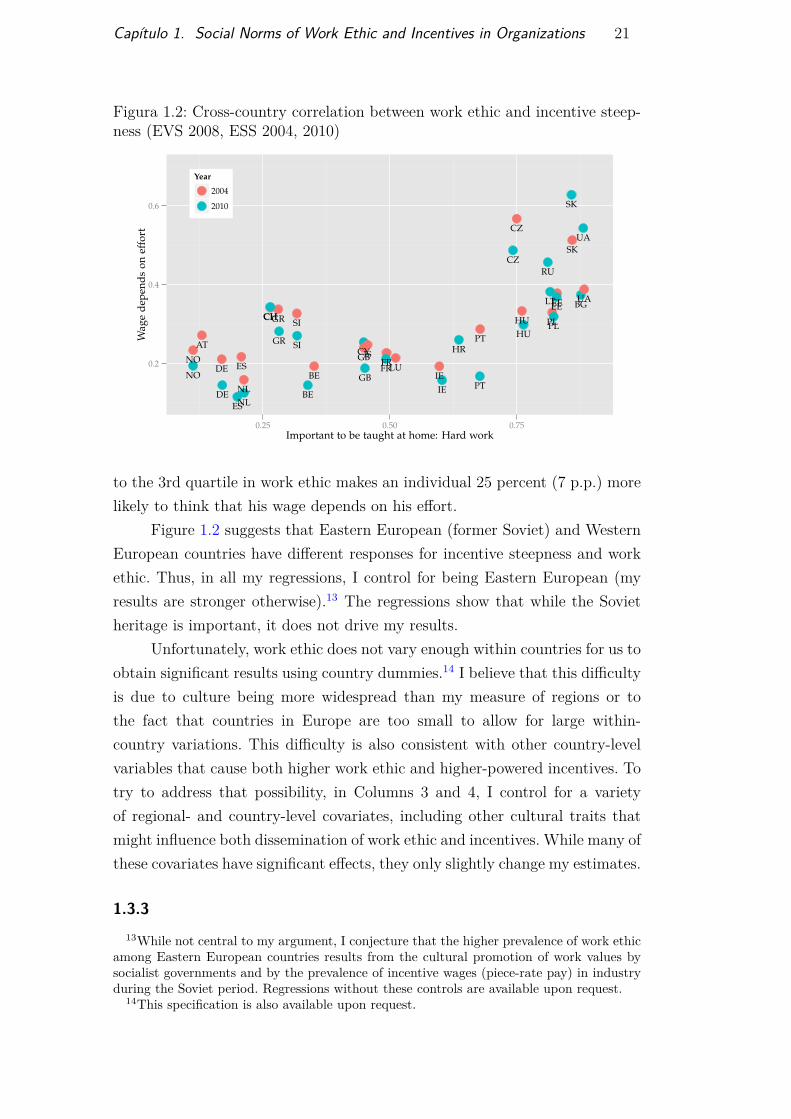
Capítulo 1. Social Norms of Work Ethic and Incentives in Organizations 21
Figura 1.2: Cross-country correlation between work ethic and incentive steep-ness (EVS 2008, ESS 2004, 2010)
AT
BE
BE
BG
HRCY
CZ
CZ
EEEE
FRFRDE
DE
GR
GR
HUHU
IS
IE
IE
LT
LU
NLNL
NO
NO
PLPLPT
PT
RU
SK
SK
SI
SI
ES
ES
CHCH
UA
UA
GB
GB
0.2
0.4
0.6
0.25 0.50 0.75Important to be taught at home: Hard work
Wag
ede
pend
son
effo
rt
Year
2004
2010
to the 3rd quartile in work ethic makes an individual 25 percent (7 p.p.) morelikely to think that his wage depends on his effort.
Figure 1.2 suggests that Eastern European (former Soviet) and WesternEuropean countries have different responses for incentive steepness and workethic. Thus, in all my regressions, I control for being Eastern European (myresults are stronger otherwise).13 The regressions show that while the Sovietheritage is important, it does not drive my results.
Unfortunately, work ethic does not vary enough within countries for us toobtain significant results using country dummies.14 I believe that this difficultyis due to culture being more widespread than my measure of regions or tothe fact that countries in Europe are too small to allow for large within-country variations. This difficulty is also consistent with other country-levelvariables that cause both higher work ethic and higher-powered incentives. Totry to address that possibility, in Columns 3 and 4, I control for a varietyof regional- and country-level covariates, including other cultural traits thatmight influence both dissemination of work ethic and incentives. While many ofthese covariates have significant effects, they only slightly change my estimates.
1.3.313While not central to my argument, I conjecture that the higher prevalence of work ethic
among Eastern European countries results from the cultural promotion of work values bysocialist governments and by the prevalence of incentive wages (piece-rate pay) in industryduring the Soviet period. Regressions without these controls are available upon request.
14This specification is also available upon request.
Capítulo 1. Social Norms of Work Ethic and Incentives in Organizations 22
Tabela 1.2: European Values Study and European Social Survey (EVS 2008, ESS2004, 2010)
(1) (2) (3) (4)Work imp. (region) 0.1304 0.1430 0.1473 0.1143
(0.0285)*** (0.0295)*** (0.0349)*** (0.0327)***Female -0.0584 -0.0596 -0.0603
(0.0073)*** (0.0072)*** (0.0072)***Education (yrs) 0.0002 -0.0009 -0.0007
(0.0014) (0.0013) (0.0013)Self-employed 0.6070 0.6000 0.5937
(0.0428)*** (0.0546)*** (0.0637)***Left-right (region) -0.0522 -0.0522
(0.0157)*** (0.0140)***Bribe just (region) 0.0660 0.0722
(0.0547) (0.0524)GDP pc (region) -0.0162 -0.0002
(0.0128)** (0.0143)Education (region) 0.0618 0.0447
(0.0162)*** (0.0157)**GDP pc (country) -0.0549
(0.0314)**Industry % (country) 0.0022
(0.0012)East-west (east) 0.1217 0.1138 0.1242 0.1138
(0.0174)*** (0.0199)*** (0.0227)*** (0.0224)***Year (2010) -0.0286 -0.0214 -0.0240 -0.0313
(0.0087)* (0.0125) (0.0118)* (0.0120)**
Country-level controls N N N YRegion-level controls N N Y YIndividual-level controls N Y Y YR2 0.040 0.085 0.093 0.095N 34375 16677 16664 16664The dependent variable is the respondent’s answer to the following question: "Please tellme how true each of the following statements is about your current job: my wage or salarydepends on the amount of effort I put into my work."I code "Very True"or "Quite True"asone and zero otherwise. Corrected standard errors are clustered at the regional level.P-values are significant at the 0.05 (*), 0.01 (**), and 0.001 (***) levels. Individual-levelcontrols are religion, gender, age, age squared, years of education, employment relation,NACER2-level industry controls, and whether there is a child at home. Region-levelcontrols are (log) income per capita (PPP), average years of education, average politicalleaning (left or right), response to whether bribes are sometimes justified, average concernfor others, response to whether freedom or equality is more important, and opinionabout the government. Country-level controls are (log) GDP per capita and industryparticipation. There are 30 countries in the sample.
Capítulo 1. Social Norms of Work Ethic and Incentives in Organizations 23
World Values Survey and Execucomp
Finally, in my third empirical exercise (Table 1.3), I test the relationbetween work ethic and steepness of incentives, without relying on self-reportedmeasures of the latter. To do so, I use Standard and Poor’s Execucompdatabase on executive compensation in the US. I match those data with USregional data from the World Values Survey (WVS). Execucomp providesdata for all S&P 1500 firms since 1994. I gather these detailed executiveearnings data to create measures of incentive steepness. Obtaining reliablemeasures of incentive steepness is difficult for the majority of the population,as their contracts usually involve efficiency wages and career concerns. Datafor executive compensation, however, is widely available, distinguished byincentive type, and as most executives receive bonuses, more reliable.
I use the WVS waves from 1995, 1999, and 2006. I match the data foreach wave to the executive data from the year before the survey, the year ofthe survey, and the year after the survey (e.g., for the first wave, I use 1994,1995, and 1996).15 A difficulty with this dataset is that I only have data onwork ethic by region.16 Still, as I have data for all three waves and for nineyears of executive compensation, it is possible to obtain precise estimates, evenwhen controlling for regional fixed effects.
In Columns 1, 2, 4, and 6, I use bonuses as a proportion of bonuses andwages as a measure of incentive steepness. Compared to the base specificationin Column 1, increasing the controls in Column 2 increases the point estimates,suggesting that the simple correlations are downward biased. In Columns 3 and5, I take into account that good executives might try to protect themselvesfrom risk and consider options and other incentive packages. My measure ofincentive steepness is then 1 − wage
total payment . These results are weaker but stillconsistent with my hypothesis. In Column 4, my preferred specification, anincrease from the first to the third quartile in regional work ethic increases theproportion of bonuses in the compensation contract by 1.5 p.p., a five percentincrease over the mean.
I use very specific industry-level controls to address the possibility thatI am capturing different compensation behaviors from different industriesthat are spatially sorted. Furthermore, the analysis considers within-countryvariation therefore controlling for country-level institutional features, but italso controls for regional fixed effects using temporal variation. Columns 4 and
15The results are robust to using executive data only for the year of the wave and usingonly some of the waves.
16Ten regions are included in the data: East South Central, West South Central, NewEngland, South Atlantic, East North Central, West North Central, Rocky Mountain States,Middle Atlantic States, Northwest and California.
Capítulo 1. Social Norms of Work Ethic and Incentives in Organizations 24
Tabe
la1.3:
WVSforUSA
andEx
ecuc
omp(W
VS19
95,1
999,
2005
,Execu
comp19
94-200
6)(1)
(2)
(3)
(4)
(5)
(6)
Workim
p.(region)
0.1386
0.21
560.16
200.1884
0.09
820.09
75(0.058
4)*
(0.091
2)*
(0.074
7)*
(0.0625)**
(0.0622)
(0.044
5)*
Age
0.00
820.0201
0.00
840.02
000.16
09(0.001
7)**
*(0.001
4)**
*(0.001
6)**
*(0.001
5)**
*(0.159
6)Age
squa
red
-0.0001
-0.000
2-0.000
1-0.000
2-0.001
5(0.000
0)**
*(0.000
0)**
*(0.000
0)**
*(0.000
0)**
*(0.001
5)Interlo
ck-0.050
7-0.067
1-0.050
7-0.068
7(0.020
6)*
(0.019
8)**
*(0.021
4)*
(0.003
0)**
*CEO
(no)
-0.032
6-0.0641
-0.032
9-0.064
70.12
41(0.002
5)**
*(0.003
2)**
*(0.002
6)**
*(0.0035)
†(0.259
7)
Year
dummies
YY
YY
YY
RegionFE
NN
NY
YN
Executivecontrols
NY
YY
Y*
R2
0.18
90.34
50.18
10.35
00.18
60.81
9N
60518
2949
229
319
29492
2931
930
The
depe
ndentvaria
blein
Colum
ns1,
2,4,
and6is
BO
NU
SB
ON
US+
SALA
RY.F
orColum
ns3an
d5,
thede
pend
ent
varia
bleis
1−SA
LAR
YT
OTA
LW
AG
E.P
-value
sare
signific
anta
tthe
0.05
(*),0.01
(**),a
nd0.001(***)levels.Fo
reach
wavetof
theW
VS,
Iuse
executivecompe
nsationda
tafort
heyears{t−
1,t,t+
1}.E
xecu
tive-levelc
ontrols
areage,
agesqua
red,
gend
er,b
eing
theCEO
,being
theCFO
,whe
ther
thebo
ardisinterlo
cked
,and
detaile
dSIC
indu
stry
code
s.Allstan
dard
errors
areclusteredat
theregion
allevel.The
last
columnag
gregates
the
varia
bles
byregion
andW
VSyear.G
iven
thesm
alln
umbe
rofo
bservatio
ns,I
removed
gend
er,interlock,a
ndSIC
code
s.The
reare10
region
sin
thesample.
Capítulo 1. Social Norms of Work Ethic and Incentives in Organizations 25
5 show that controlling for regional fixed characteristics has small effects onthe estimated coefficients.
The coarse nature of the regional data might call into question therobustness of the results. In column 6, I apply the most challenging testpossible: I aggregate the observations by WVS wave and region, obtaining30 observations (three waves for each of the ten regions). Surprisingly, thecorrelation still holds. (In this specification, I have to drop the interlock andgender variables to maintain statistical power.)17 I believe that this supportsthe robustness of the empirical results of this exercise.
Finally, using executive compensation raises the question of how theresults generalize to the rest of the working population. I hope that futureresearch will use better data and be able to test the implications of my modelmore carefully, focusing on causal identification and external validity.
1.4Model
In my model, there is a population of measure two consisting of over-lapping generations of agents that live two periods. In the first period, theyacquire by a cultural transmission process a binary trait k ∈ {W,N} that in-dicates the presence (W ) or absence (N) of a work ethic. In the second period,they are employed (and remunerated) by a firm and choose whether to instilla work ethic in their offspring. For simplicity, I assume that reproduction isasexual and that each individual has exactly one child. Hence, the measure ofadults in the population is one, and I denote the proportion of adults with awork ethic as xW .
I assume that the work-related decisions and the cultural transmissionchoice are separable and consider them separately. I start by analyzing thefirm problem.
1.4.1Moral Hazard in Teams Game
I model employment in firms as a moral hazard in teams game. There isa continuum of measure one of firms, each being matched with two randomlychosen individuals from the population to engage in production each period.18
I assume that each firm employs its two agents in a project with value ρ, and17These variables suffer from excessively high homogeneity. Only 5% of executives in my
sample are female, and 1.7% of boards are interlocked. I also drop the SIC industry controlsgiven their number.
18Consider, for example, that firm f is matched with agents f/2 and (f+1)/2, which is anunique matching almost everywhere.
Capítulo 1. Social Norms of Work Ethic and Incentives in Organizations 26
the probability of success is given by θaαi aαj , with α ∈ (0, 1), ai, aj ∈ [0, 1] andθ ∈ (0, 1]. In this equation, ai (aj) represents the effort exerted by agent i (j),and θ represents the efficiency of effort of agents i and j. With some abuse ofnotation, I will use subscripts i and j to refer to both agents and agent types.
This functional form entails that the probability of success is supermodu-lar, representing a production process in which the effort of workers is comple-mentary. An example is an assembly-line production plant, where the producti-vity of a worker is directly related to the speed at which he receives productioninputs, which are the outputs produced by the previous workers in that line.
As employee effort is non-observable, the firm must choose a compensa-tion scheme that is incentive compatible. I assume that the firm has completeinformation about whether the agent has work ethic.19 Importantly, I alsoassume that there are institutional constraints that forbid a negative wage(i.e., limited liability). Limited liability is essential to my model, as otherwisethe firm would always equal the workers’ expected payoff to the utility gai-ned by their outside option, irrespective of type. Given these assumptions,since the project outcome is binary, the firm can restrict its attention to linearincentive schemes formed by a bonus b for each combination of types, viz.,{bij}i,j∈{W, N}.20 Both workers and firms are risk neutral.
Agents have a quadratic cost of effort that depends on the traits theyacquired during their childhoods. Those with a work ethic have a lower mar-ginal cost of effort κWai than workers without it (κNai)—namely, κW < κN—representing the moral justification for effort that eases their toil. However,work ethic entails costs beyond those related to work. For example, in religiousthought, while the promise of eternal recompense for hard work (as expressedin the epigraph) can ease the cost of effort, it cannot be dissociated from theascetic view that leisure and comfort are worthy of "absolute moral condem-nation,"as Baxter claims. To account for this, I assume that agents with workethic suffer a cost KW that is exogenous to their work behavior, indicating aninability to enjoy free time with family and friends.21
Accordingly, the utility of an agent of type i with a coworker of type j(defining IA as the indicator function of A) is:
19I discuss this and other main assumptions of my model in the next section.20Restricting the compensation scheme to a bonus without a base wage is without loss of
generality given limited liability if the outside option is not too high (e.g., if it is zero).21Since κW < κN , without the cost KW , it would always be advantageous to acquire a
work ethic (in my specification of cost linear in types). This is the simplest specification,which implies that for low effort, having a work ethic is worse, while for high effort it isadvantageous; this result fits the concept of work ethic as motivated in Section 2. Intuitively,this fixed cost KW represents the costs of having a work ethic that are unrelated to workbehavior, such as the lower utility derived from consumption and leisure time (e.g., vacations)or worse social relations.

Capítulo 1. Social Norms of Work Ethic and Incentives in Organizations 27
(θaαi a
αj
)bij − I{i=W}KW − κi
a2i
2 . (1-1)
Moreover, throughout the paper I assume that the outside option isredundant given limited liability, (viz., the outside option u ≤ 0). Addinga binding outside option (as long as it is not high enough to make the modeltrivial) would not change the results.
The firm chooses the optimal incentive scheme to maximize its profit,knowing that the agents choose their effort in an incentive compatible waygiven the proposed scheme. Here, a(b; κi, aj) denotes the effort a worker exertswhen faced with bonus b, having type κi and coworkers with effort aj, that is:
a(b; κi, aj) = argmaxa
(θaαaαj
)b− I{i|i=W}KW − κi
a2
2 .
Then, the problem of the firm is given by:
maxbij , bji
θaiaj (ρ− bij − bji) , such that ai = a(bij, κi, aj) and aj = a(bji, κj, ai).(1-2)
Since effort is complementary, when an agent has a hard-working cowor-ker, his own effort becomes more productive, and the firm will choose to incen-tivize him to work harder as well. In fact, defining a∗i (κi, κj) as the equilibriumeffort choice of an employee of type i with a coworker of type j, the optimalincentive scheme is such that the effort is given by:
a∗i (κi, κj) =[θρα2a∗j(κj, κi)α
2κi
]A= (θρα2)1+αA
21+αAκiκαAj
A1−α2A2
, (1-3)
where A = 12−α . Intuitively, an agent with a higher cost of effort is costlier to
incentivize, and in equilibrium, he will work less. More importantly, as workeffort is complementary, having a coworker who exerts low effort reduces anagent’s productivity, inducing the firm to offer lower bonuses and thus elicitlower effort.
The second part of equation (1-3) presents the optimal effort choice asa function of the agents’ traits. Workers without a work ethic and workerswhose peers do not have a work ethic work less in equilibrium. Even moreinterestingly, while all individuals work harder when their peers have a workethic, this difference is greater for workers who have a work ethic themselves.The same is true for the total compensation received by workers: an individualmatched to a peer with a work ethic receives higher compensation than onematched to a coworker without a work ethic, but this effect is greater forindividuals who have a work ethic themselves (this can be seen by noting that
Capítulo 1. Social Norms of Work Ethic and Incentives in Organizations 28
the compensation received by an agent is a convex function of his effort).22
The main result of this section establishes that the same is true forutilities: it is always beneficial to have coworkers with a strong work ethic,but this benefit is higher for workers who have a work ethic themselves.Symmetrically, having a work ethic is especially advantageous when theindividual is likely to enjoy a hardworking coworker. Intuitively, in a productionline, the faster the inputs reach a worker’s station, the faster that employeecan work. However, this is only useful inasmuch as she can produce at leastas fast as the inputs arrive (by exerting enough effort). For fast workers, theadvantage of being in a fast production line (when earning piece rates) is verylarge, while for a slow worker, it is negligible.
I now proceed to formally state the main result of this section, which isdiscussed above. For that, I define the matching payoff of a worker of typei when matched with a coworker of type j as the utility she receives underthe optimal compensation scheme, given her coworker’s type. I denote it asV (i, j).
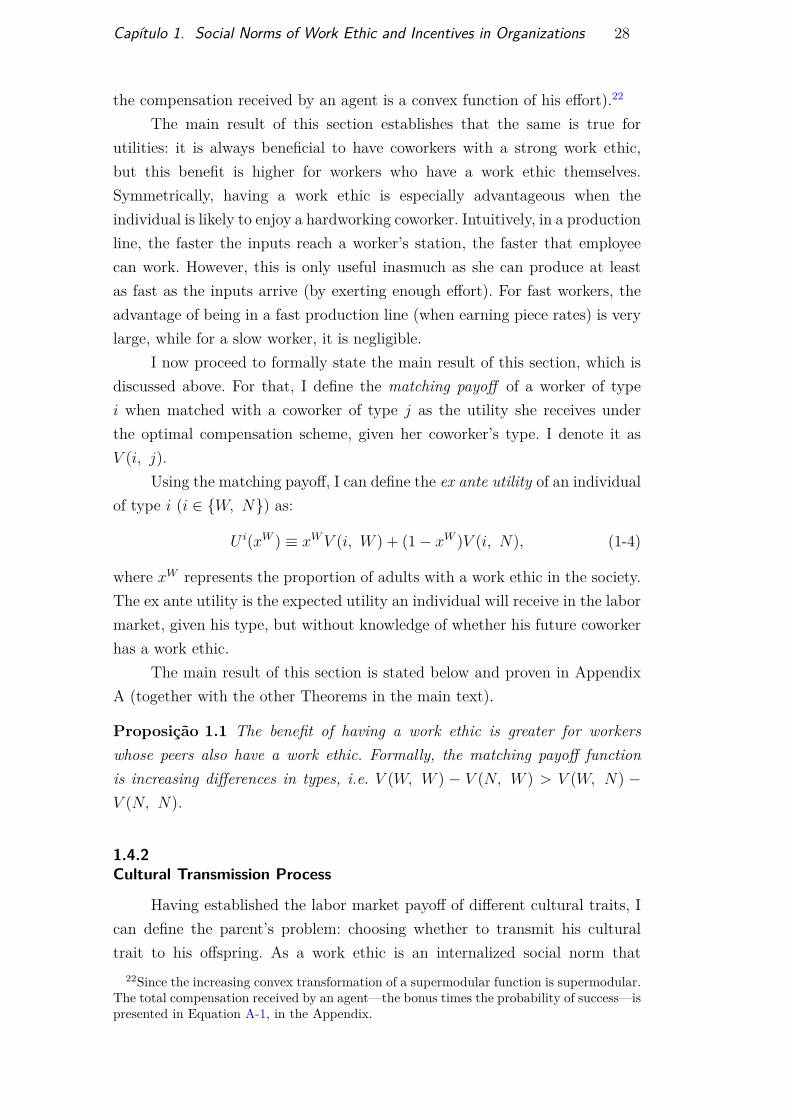
Using the matching payoff, I can define the ex ante utility of an individualof type i (i ∈ {W, N}) as:
U i(xW ) ≡ xWV (i, W ) + (1− xW )V (i, N), (1-4)
where xW represents the proportion of adults with a work ethic in the society.The ex ante utility is the expected utility an individual will receive in the labormarket, given his type, but without knowledge of whether his future coworkerhas a work ethic.
The main result of this section is stated below and proven in AppendixA (together with the other Theorems in the main text).
Proposição 1.1 The benefit of having a work ethic is greater for workerswhose peers also have a work ethic. Formally, the matching payoff functionis increasing differences in types, i.e. V (W, W ) − V (N, W ) > V (W, N) −V (N, N).
1.4.2Cultural Transmission Process
Having established the labor market payoff of different cultural traits, Ican define the parent’s problem: choosing whether to transmit his culturaltrait to his offspring. As a work ethic is an internalized social norm that
22Since the increasing convex transformation of a supermodular function is supermodular.The total compensation received by an agent—the bonus times the probability of success—ispresented in Equation A-1, in the Appendix.
Capítulo 1. Social Norms of Work Ethic and Incentives in Organizations 29
directly affects the preferences of individuals, I follow the literature on theintergenerational transmission of cultural norms established by (28), (29), and(01, 02).
Parents of type i choose a socialization effort di ∈ [0, 1] in an attemptto pass their trait on to their offspring. This socialization effort succeedswith probability di, in which case the offspring will acquire the parental trait(vertical socialization). If this effort is unsuccessful, the child will acquire thetrait of a random element of the population (horizontal/oblique socialization).In that case, the probability that the trait acquired is the same as the father’sis xi, where xi is the proportion of trait i in the society.
Concisely, the probability that a child of a parent of type i acquires traiti (resp., j) is given by:
P ii(di; xi) = di + (1− di)xi
P ij(di; xi) = (1− di)(1− xi).
Parents are altruistic and consider their offspring’s expected labor marketutility when deciding whether to transmit a work ethic. As shown in theprevious section, the moral hazard in teams problem entails that the ex anteutility of having a work ethic is a function of the (beliefs about the future)proportion of individuals in the population with a work ethic. I assume,however, that parents are myopic: they choose their socialization effort basedon the dissemination of work ethic they observe themselves in the society. Thiscan be seen as a form of imperfect altruism, in the sense that parents observetheir own environment and payoff when considering their children’s utility.
This form of imperfection is not the same as that in (01). There, theyassume exogenous cultural intolerance, and they propose imperfect altruism inthe form of a parental view that their own traits always produce higher utilityfor their offspring. (Intuitively, it represents a case in which parents cannotteach what they do not believe.) I consider my assumption a generalization oftheirs to a scenario wherein the dissemination of a trait influences the payoffsof the agents directly.
Moreover, in Bisin & Verdier (2000), it is natural to impose the conditionthat parents can only socialize children to value their own traits, as they wouldnever want to do otherwise. In my model, I impose the same condition forsimplicity of exposition, with the intuition that a parent cannot pass on abelief that she does not share herself. In my model, a deeply religious parentcannot teach her offspring to disregard religion, as it would go against herbeliefs. She can, however, exert little effort in socializing her offspring, as it

Capítulo 1. Social Norms of Work Ethic and Incentives in Organizations 30
will not be advantageous for her child to be religious given the cultural valuesof the society.23
Given the cultural transmission process, parents of type i maximize withregards to socialization effort di:
P ii(di; xi)U i(xW ) + P ij(di; xi)U j(xW )− (di)2
2 ,
where U i is the ex ante utility of the individual of type i introducedin the last section. The first order conditions imply that dW = max{(1 −xW )∆U(xW ), 0}. As in the literature, I call ∆U(xW ) ≡ UW (xW ) − UN(xW )the cultural intolerance of work ethic. As is clear in equation (1-4), culturalintolerance is endogenous: it depends on the proportion of the population witha work ethic. Moreover, Proposition 1.1 states that individuals with a workethic gain more by having a peer with work ethic than do individuals withoutthat trait. Hence, this is a game of strategic complements, and my culturaltransmission process is a process of cultural conformity (see (13)). I formalizethis assertion in Proposition 1.2 below.
Proposição 1.2 Assume that parameters are not such that it is always betteror always worse for an agent to have a work ethic, independently of who heworks with. Then, there exists x∗ ∈ (0, 1) such that if the dissemination ofwork ethic at a moment t, xWt , is less than x∗, the proportion of individuals witha work ethic converges to zero, and if xWt is larger than x∗, then it convergesto one.
Figure 1.3 below illustrates Proposition 1.2 for a set of example para-meters. In societies with low dissemination of work ethic, parents expect thattheir children are more likely to be employed with low-effort coworkers and bepaid low-powered wages. As such, they find it in their offspring’s best interestto transmit cultural traits that oppose having a work ethic—that is, that pro-mote leisure and the importance of personal life rather than that of a career.However, in societies with high dissemination of work ethic, the average com-pensation scheme is high-powered, so the returns to high effort are large. Inthat case, parents will altruistically choose to disseminate work ethic, propa-gating beliefs that work is important and that it provides a purpose in life (acalling).
23Nonetheless, I note that this has no effect on the results (except to change the ratesof convergence of different dynamic equilibria). Indeed, one would obtain similar results bysubstituting this cultural transmission process with properly defined replicator dynamics. Irefrain from doing so, however, because this model provides a more intuitive representationof the intergenerational transmission of cultural values.
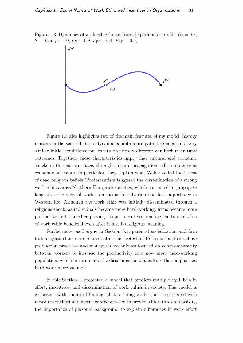
Capítulo 1. Social Norms of Work Ethic and Incentives in Organizations 31
Figura 1.3: Dynamics of work ethic for an example parameter profile. (α = 0.7,θ = 0.25, ρ = 10, κN = 0.8, κW = 0.4, KW = 0.6)
0.5 1
x∗ xW
xW
Figure 1.3 also highlights two of the main features of my model: historymatters in the sense that the dynamic equilibria are path dependent and verysimilar initial conditions can lead to drastically different equilibrium culturaloutcomes. Together, these characteristics imply that cultural and economicshocks in the past can have, through cultural propagation, effects on currenteconomic outcomes. In particular, they explain what Weber called the "ghostof dead religious beliefs."Protestantism triggered the dissemination of a strongwork ethic across Northern European societies, which continued to propagatelong after the view of work as a means to salvation had lost importance inWestern life. Although the work ethic was initially disseminated through areligious shock, as individuals became more hard-working, firms became moreproductive and started employing steeper incentives, making the transmissionof work ethic beneficial even after it lost its religious meaning.
Furthermore, as I argue in Section 6.1, parental socialization and firmtechnological choices are related: after the Protestant Reformation, firms choseproduction processes and managerial techniques focused on complementaritybetween workers to increase the productivity of a now more hard-workingpopulation, which in turn made the dissemination of a culture that emphasizeshard work more valuable.
In this Section, I presented a model that predicts multiple equilibria ineffort, incentives, and dissemination of work values in society. This model isconsistent with empirical findings that a strong work ethic is correlated withmeasures of effort and incentive steepness, with previous literature emphasizingthe importance of personal background to explain differences in work effort
Capítulo 1. Social Norms of Work Ethic and Incentives in Organizations 32
across regions and stylized facts in the literature pointing to the significantimportance of effort exertion in explaining productivity differentials acrossnations and periods. In the next section, I discuss some assumptions of mymodel, and in Section 6, I extend it to include the firm technological choice.
1.5Discussion
In this section, I discuss some of the assumptions and results of mymodel. First, I argue that the assumption that the firm knows the workers’types and can discriminate among them when devising the incentive schemeis reasonable. Then, I argue that incentive schemes based only on bonusesimply no loss of generality, even though only a small fraction of the work forceactually receives incentive wages. Finally, I discuss complementarity of effortand welfare consequences of the model.
To motivate common knowledge of types, imagine that the firm canobserve the output y of an agent in each period but not the effort. If theeffort is constant, as in my model, then by observing the output a sufficientnumber of times, the firm can infer the type of the agent, with arbitrarily smalldegree of uncertainty. As a result, if the contractual relationship is sufficientlylong, it is with no loss of generality to suppose that the firm knows the typeof agent, even if it cannot observe the effort the agent supplies at any giventime.
Moreover, if the firm not only pays bonuses when the output is realizedbut also adjusts their wages (for example, through raises), then over time, it canmake the payment of different types of agents converge to their optimal valuesby choosing an appropriate adjustment rule, even if direct discrimination isforbidden or discouraged. Therefore, there is no loss of generality in assumingthat firms can freely choose incentive schemes contingent on workers’ types.
Another assumption of the model is that firms rely solely on incentivewages to elicit effort, while in actuality, many other types of incentives areavailable, most commonly, career concerns and efficiency wages. While mymodel does not explicitly account for these other forms of incentives, theintuition is the same, and the generalization would be straightforward. Asa result, although my model considers only piece-rate workers, my argumentis general.
Importantly for the interpretation of the model, the incentive schemepaid by the firm to an agent of type i with coworkers of type j is:
Capítulo 1. Social Norms of Work Ethic and Incentives in Organizations 33
bij(κi, κj) = κiθα
(θρα2)1+αA
21+αAκiκαAj
(2−α)A1−α2A2
(θρα2)1+αA
21+αAκjκαAi
− αA1−α2A2
(1-5)
Regarding the effect of having a coworker with a strong work ethic, thereare two opposing forces at work. On the one hand, since the marginal costof effort is lower, for a given level of effort, the firm needs to compensate theworker less, reducing the bonus. On the other hand, the firm wants to elicitmore effort from a now more productive worker and thus needs to pay hima larger bonus for that effort. Equation (1-5) shows that the second effect isstronger: a lower cost of effort for a worker and for his coworker results inhigher bonuses, that is, higher-powered incentives. In this sense, my modelpredicts that societies with a more broadly disseminated work ethic havehigher-powered incentives.
A hallmark of the model is that work effort is complementary. Comple-mentarity is a topic that has received increasing attention in the literatureon organizational economics (e.g., (33), (26), (25)). Although observationalevidence points to effort complementarity as an important part of modernproduction processes (for example, Fordism and lean manufacturing), so far,it has not been an important part of models of organizational behavior.
One reason is that incorporating complementarity causes significant los-ses of tractability in models of moral hazard, and in this regard, another contri-bution of this paper is to suggest a tractable model of effort complementarity.A second is that obtaining causal evidence on the existence of complementa-rity is difficult. Observational data that corroborates the existence of sortingon worker diligence among sectors and firms notwithstanding, it is difficult todisentangle the effects of effort complementarity from those of other explana-tions.
Nevertheless, including complementarity in the model has an appealingimplication. In the model, a worker’s income depends on the effort chosen byhis coworkers, which is consistent with differing wages across firms and sectorsand correlated within a firm, a features that one observes empirically. (27), forexample, notes that occupation and employer identity explain 90 percent ofthe observed variation in wages.
The model has well-defined implications for welfare, although welfarecomparisons in models with changing preferences are notoriously problematic(see (23)). According to Proposition 1.2, there are only two asymptoticallystable dynamic equilibria: one with a fully disseminated work ethic and one inwhich there is no work ethic in the society. Welfare analysis is thus reduced tocomparing these two equilibria.
Capítulo 1. Social Norms of Work Ethic and Incentives in Organizations 34
Indeed, in the model, the dynamic equilibria (of Proposition 1.2) areranked in terms of welfare, as all workers (and firms) prefer to have coworkerswith a strong work ethic. In a more basic sense, having coworkers with awork ethic results in a higher probability of success, even if the worker’s owneffort is constant. More subtly, it makes the agent more productive, and moreproductive agents work harder, receive larger shares of the surplus, and havehigher utilities. My model, therefore, represents a world in which effort pays:individuals who work harder have higher utilities.24 Hence, for any parameterprofile for which it is not always worse to have a work ethic, the equilibriumwith full dissemination of a strong work ethic is more efficient, based on theargument above and Proposition 1.1, V (W, W ) > V (N, W ) > V (N, N).
1.6Extensions
In this section, I analyze possible extensions to my benchmark model. Aquestion raised by the previous analysis is why firms in societies with limiteddissemination of work ethic would choose complementary technologies, as thiscauses a decrease in productivity. In Section 6.1, I augment the base model toaccount for the firm technology choice, and I show that firms in low work ethicsocieties indeed prefer non-complementary technologies. Moreover, if stronglycomplementary technologies are interpreted as being more technologicallyadvanced than non-complementary ones (as in Fordism or lean manufactureversus more traditional forms of production), then this extension providesa rationale (akin to (22)) for the differences in technological adoption thatone observes empirically.25 In this extended model, I characterize the phasediagram induced by the firm technology choice and the parental socializationprocess. Finally, in Section 6.2, I show how the dynamic equilibria of this modelrespond to changes in the underlying parameters to better comprehend whysome regions have a widely disseminated work ethic while others do not.
24It is important to note that this is in fact a general property of moral hazard problemswith limited liability. To see this, consider a general moral hazard problem with a workerwho has utility function by(a) − c(a) and works for a firm with profit y(a)(1 − b), where ais effort and b a bonus for success. Then, note that the total derivative of the agent’s utilityin regards to effort (repaid through optimal incentives) is:
duda (a) = c′′(a)y′(a)− c′(a)y′′(a)
y′(a)2 y(a),
which represents how much better off an agent is by working (in equilibrium) more, forexample, because of higher productivity. It is positive under the very standard assumptionsthat y is increasing and concave and c is increasing and convex.
25In this section, my argument is similar to (22). However, besides my focus on culture, Istudy the effort choice of the workers and endogenize the compensation choice of the firms,while their model is based on sorting on skill.

Capítulo 1. Social Norms of Work Ethic and Incentives in Organizations 35
1.6.1Firm Selection
In the extended model, firms can choose a technology q ∈ {C, S}, whereC stands for the complementary technology presented in the base model, and Sstands for a separable technology in which the project is divided in two separatetasks, each with a value γρ, and employing a single worker with successprobability θaαi , where γ is the relative productivity of the complementary andseparable sectors of the economy. If one portrays these sectors as representingmodern and traditional industries, respectively, then γ corresponds to theirrelative productivity. Therefore, one would expect that events such as theIndustrial Revolution change γ (namely, they decrease it), affecting firm (andindirectly parental) choices.
I assume that there is a lump sum cost of complementary technologiesζ, as these technologies are more modern and expensive production processes(both to acquire and to maintain).
In a firm with separable technology, the utility that agent i receives isindependent of the effort (or type) of his coworker and is given by:
(θaαi ) bi − κia2i
2 (1-6)
Furthermore, as opposed to when employed by firms with complemen-tarity, the effort chosen by an agent of type i when faced with the separabletechnology firm’s incentive scheme depends only on his own type. It is givenby:
a∗i (κi) =[ργθα2
2κi
]A(1-7)
I denote the proportion of firms with complementary technology in theeconomy by βC , and I assume that competition among firms causes low-achieving ones to be replaced by new entrants. Specifically, I consider the firms’fitness to be proportional to their revenue relative to the mean revenue in thesociety.26 I model the selection process as a (discrete) replicator dynamic witha speed-scaling parameter s. Denoting by Y (βCt , xWt ; q) the expected revenue(net of complementary process cost ζ) of a firm with technology q ∈ {C, S}in period t, the proportion of firms with complementary technology in periodt+ 1 is then given by:
βCt+1 − βCt = sβCt
Y (βCt , xWt ; C)−∑
q∈{C, S}βqt Y (βCt , xWt ; k)
(1-8)
26I use revenue instead of profits as a selection mechanism because it is more tractable, asprofits are a highly nonlinear function of the agents’ types, and clarifies the interpretation.
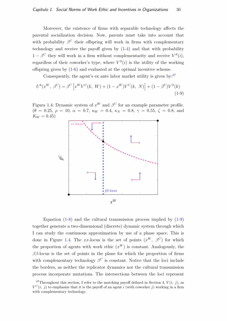
Capítulo 1. Social Norms of Work Ethic and Incentives in Organizations 36
Moreover, the existence of firms with separable technology affects theparental socialization decision. Now, parents must take into account thatwith probability βC their offspring will work in firms with complementarytechnology and receive the payoff given by (1-4) and that with probability1 − βC they will work in a firm without complementarity and receive V S(i),regardless of their coworker’s type, where V S(i) is the utility of the workingoffspring given by (1-6) and evaluated at the optimal incentive scheme.
Consequently, the agent’s ex ante labor market utility is given by:27
Uk(xW , βC) = βC[xWV C(k, W ) + (1− xW )V C(k, N)
]+ (1− βC)V S(k)
(1-9)
Figura 1.4: Dynamic system of xW and βC for an example parameter profile.(θ = 0.25, ρ = 10, α = 0.7, κW = 0.4, κN = 0.8, γ = 0.55, ζ = 0.8, andKW = 0.45)
xx locus
ββ locus
xW
βC
Equation (1-8) and the cultural transmission process implied by (1-9)together generate a two-dimensional (discrete) dynamic system through whichI can study the continuous approximation by use of a phase space. This isdone in Figure 1.4. The xx-locus is the set of points (xW , βC) for whichthe proportion of agents with work ethic (xW ) is constant. Analogously, theββ-locus is the set of points in the plane for which the proportion of firmswith complementary technology βC is constant. Notice that the loci includethe borders, as neither the replicator dynamics nor the cultural transmissionprocess incorporate mutations. The intersections between the loci represent
27Throughout this section, I refer to the matching payoff defined in Section 4, V (i, j), asV C(i, j) to emphasize that it is the payoff of an agent i (with coworker j) working in a firmwith complementary technology.
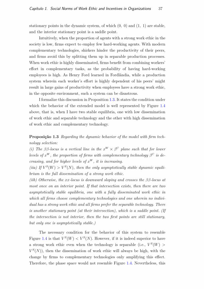
Capítulo 1. Social Norms of Work Ethic and Incentives in Organizations 37
stationary points in the dynamic system, of which (0, 0) and (1, 1) are stable,and the interior stationary point is a saddle point.
Intuitively, when the proportion of agents with a strong work ethic in thesociety is low, firms expect to employ few hard-working agents. With moderncomplementary technologies, shirkers hinder the productivity of their peers,and firms avoid this by splitting them up in separable production processes.When work ethic is highly disseminated, firms benefit from combining workers’effort in complementary tasks, as the probability of having hard-workingemployees is high. As Henry Ford learned in Fordlândia, while a productionsystem wherein each worker’s effort is highly dependent of his peers’ mightresult in large gains of productivity when employees have a strong work ethic,in the opposite environment, such a system can be disastrous.
I formalize this discussion in Proposition 1.3. It states the condition underwhich the behavior of the extended model is well represented by Figure 1.4above, that is, when I have two stable equilibria, one with low disseminationof work ethic and separable technology and the other with high disseminationof work ethic and complementary technology.
Proposição 1.3 Regarding the dynamic behavior of the model with firm tech-nology selection:(i) The ββ-locus is a vertical line in the xW × βC plane such that for lowerlevels of xW , the proportion of firms with complementary technology βC is de-creasing, and for higher levels of xW , it is increasing.(iia) If V S(W ) > V S(N), then the only asymptotically stable dynamic equili-brium is the full dissemination of a strong work ethic.(iib) Otherwise, the xx-locus is downward sloping and crosses the ββ-locus atmost once on an interior point. If that intersection exists, then there are twoasymptotically stable equilibria, one with a fully disseminated work ethic inwhich all firms choose complementary technologies and one wherein no indivi-dual has a strong work ethic and all firms prefer the separable technology. Thereis another stationary point (at their intersection), which is a saddle point. (Ifthe intersection is not interior, then the two first points are still stationary,but only one is asymptotically stable.)
The necessary condition for the behavior of this system to resembleFigure 1.4 is that V S(W ) < V S(N). However, if it is indeed superior to havea strong work ethic even when the technology is separable (i.e., V S(W ) >
V S(N)), then the dissemination of work ethic will always be high, with thechange by firms to complementary technologies only amplifying this effect.Therefore, the phase space would not resemble Figure 1.4. Nevertheless, this
Capítulo 1. Social Norms of Work Ethic and Incentives in Organizations 38
would be contrary to the argument (presented in Section 2) that a work ethicwas absent in Medieval Europe, having emerged instead during the ProtestantReformation and Industrial Revolution.
1.6.2Comparative Dynamics
In this section, I discuss how the dynamic equilibria are affected bychanges in the basic parameters of the model. Because the cultural transmissionprocess and the replicator dynamics of firm selection have no mutations, inany asymptotically stable equilibrium (namely, (0, 0) and (1, 1)), parameterchanges do not have any effect.28 I can, however, study how changes inparameters affect the size of the basins of attraction of the dynamic equilibria.These comparative dynamics for the extended model presented in Section 6.1are summarized in Proposition 1.4 below.
Proposição 1.4 Assume a phase space like Figure 1.4 (see Proposition 1.3).Then, an increase in human capital (θ) and in the value of project (ρ) and adecrease in the fixed cost of having a work ethic (KW ) and in the relativeproductivity of the separable sector (γ) increase the basin of attraction ofthe equilibrium with high dissemination of a strong work ethic and a highproportion of firms with complementary technology (and vice versa).
Intuitively, when workers are more productive (higher θ) or the projectthey work on is more valuable (higher ρ), firms optimally choose to offer largerbonuses, eliciting higher effort. As higher effort is less costly for individualswith a work ethic than for those without, transmitting a strong work ethicbecomes more valuable for parents. Furthermore, as more productive workersexert more effort, it also becomes advantageous for the firm to choose moderncomplementary technologies, as the gains from complementarity are increasedby higher effort. In this scenario, parents want to strongly instill a workethic in their children and firms choose more complementary technologies, andthe equilibrium with a widely disseminated work ethic and complementarytechnology becomes more likely (as in there are more initial states thatconverge to that equilibrium).
Moreover, a decrease in the cost of having work ethic KW (e.g., the moralcondemnation of leisure) makes a strong work ethic more desirable, while areduction in the relative productivity of the separable sector γ (for example,technological advancements that rely on complementarity, such as assembly
28The model can be extended to incorporate random shocks to the proportion of workerswith a strong work ethic. In that case, changes in the parameters would alter the probabilitythat the equilibrium changes. The intuition of the model would remain unchanged, however.
Capítulo 1. Social Norms of Work Ethic and Incentives in Organizations 39
Figura 1.5: Dynamic system of xW and βC (θ = 0.25, ρ = 10, α = 0.7,κW = 0.4, κN = 0.8, γ = 0.55, ζ = 0.8, and KW = 0.4)
xx locus
ββ locus
KW = 0.4
θ = 0.27
γ = 0.5
xW
βC
lines, or that disproportionately benefit more modern sectors, such as steamengines and computers) induce firms to adopt complementary technologies.Although the decrease in the cost of having a work ethic affects only theparental socialization choice directly, as the complementary technology ismore attractive when the proportion of workers with a strong work ethic ishigher, it also indirectly affects firm choice. Analogously, while changes inthe relative productivity of the two technologies directly affect only the firmsdecision, workers with a work ethic prefer to work for firms with complementarytechnologies, hence they indirectly affect their choice.
Proposition 1.4 is illustrated in Figure 1.5 in which I consecutively applychanges to the parameters of Figure 1.4 (in gray). First, a decrease in the costof having work ethic KW has the effect of lowering the xx-locus, increasingthe basin of attraction of the hard-working equilibrium. Then, an increase inproductivity θ has the effect of moving the xx-locus down and shifting theββ-locus to the left, increasing the area of dissemination of both work ethicand firms with complementarity that leads to the equilibrium with full disse-mination of both. Finally, lowering the relative productivity of the separablesector γ moves the ββ-locus left, making the hard-working equilibrium morelikely.29 While these changes are purely illustrative, I believe that they accu-rately represent the transformations that occurred during the 18th and 19thcenturies in industrialized economies, leading to the dissemination of cultu-
29A reduction of γ also has an effect of moving the xx-locus up, as it is a analogous to adecrease in ρ for the separable technology.
Capítulo 1. Social Norms of Work Ethic and Incentives in Organizations 40
ral norms of work values and the diffusion of production processes focused oncomplementarity, which one currently observes.
These comparative dynamics explain the impact of the Protestant Re-formation, which disseminated an ascetic view and stressed the importanceof hard work for (religious) salvation, lowering the cost of effort and raisingthe cost of leisure. Consequently, it enlarged the basin of attraction of theequilibrium with hard-working agents, making the dissemination of a strongwork ethic more likely. While it only affected the cultural transmission pro-cess directly, by allowing the dissemination of a work ethic, the ProtestantReformation also permitted firms to adopt more advanced technologies, usingthe new hard-working population in more complementary production proces-ses. Analogously, the Industrial Revolution, which favored modern productionprocesses, induced the adoption of new technologies, which by making effortmore complementary, also made a work ethic more desirable, facilitating itsdissemination. These two changes, therefore, had mutually reinforcing effects,creating a new equilibrium with a broadly disseminated work ethic and com-plementary technologies.
1.7Conclusion
Cultural norms of work effort have been studied in economics, but thefocus so far has been mostly on the interaction between work ethic and politicalredistribution. In this paper, I presented a model of work ethic disseminationand firm incentive choice. I showed results that are consistent with this modelin three separate empirical exercises.
While my model is not the only relevant one for understanding thecultural determinants of work behavior, it provides new insights and differentpolicy implications from those that have been established in the literaturethus far. For example, if one considers multiple equilibria in work ethic to be apurely political issue, then an exogenous change in the tax rate would changethe dissemination of work ethic in the society and move it from one equilibriumto the other. I argue in this paper that firms’ incentive steepness is related towork ethic; hence, the previous assertion does not have to be true. There mightbe societies with the same level of redistribution and different levels of workethic because of differences in (endogenously chosen) firm incentives.
I further show that if I allow firms to choose their technology and Iinterpret the complementary technology as more modern, then my modelprovides an explanation for why firms in third-world economies do not adoptmore modern practices from advanced economies: given the mean level of effort

Capítulo 1. Social Norms of Work Ethic and Incentives in Organizations 41
in the economy, technologies in which the production of one worker is highlydependent of the production of peers (e.g., when many workers manage a ringspinning textile machine) are less profitable than technologies in which workerproduction is independent (as in the putting-out system). The same argumentcan be made for why technological and productive advancement flourished in18th century northern Europe, reaching southern Europe only at the end ofthe 19th century.
I explore this point more carefully by examining how the basins ofattraction of the different equilibrium levels of work ethic change with changesin economic parameters. I find that an increase in human capital and a decreasein the cost of a work ethic, for example, from religious support for an asceticlifestyle, facilitate the expansion of both a strong work ethic and the modernsector. I believe that these comparative dynamics provide insights into theimpact of higher literacy and the Protestant work ethic on the IndustrialRevolution and on overall economic development in 18th century northernEurope.
I hope that future empirical research will further study the correlationbetween work ethic and firm compensation schemes. It would be particularlyinteresting to analyze causal effects between these variables, searching forquasi-exogenous variations in both culture and incentives and examining theirlong-term effects.

2Neighbors’ Income and Demand for Redistribution
"The problem is that sometimes when I’m ’riching’ aroundtown, I’ll accidentally catch glimpse of a non-rich person. ThenI get a funny feeling in my heart. Apparently I have an allergyto non-wealthy people called... empathy". Stephen Colbert in TheColbert Report (July 28, 2014).
2.1Introduction
A major question in Political Economy is what determines demand forredistribution in modern democracies, and why it differs so markedly betweensocieties, e.g. Europe and United States. In the recent decades a large literaturehas risen, mainly focused on explaining these differences in terms of differentperceived or real views on returns to effort and social mobility.
If perceptions of social mobility and the distribution of income are im-portant in determining demand for redistribution, then a person’s environment(and in particular the economic condition of his neighbors) should be an im-portant determinant for how much people want to redistribute. Unfortunately,this has not been sufficiently researched within the literature of Political Eco-nomy so far.
In this paper I try to provide a first step in answering that questionby using precinct-level election data for United States 2004-2012 Presidentialelections and Census block group level socioeconomic variables to analyzewhether having high or low income neighbors affects votes for Democrats,which I argue is a good measure for demand for redistribution.
While my evidence is not (quasi-)experimental, I employ a variety ofcontrols, as well as fixed effects and tract-year dummies, in order to accountfor possible endogeneity of housing decisions and political leaning. Our mainidentification hypothesis is that within an election cycle and a given tract (eachtract has, on average, four precincts—our unit of analysis), housing decisionsare random.

Capítulo 2. Neighbors’ Income and Demand for Redistribution 43
Given that my empirical strategy involves the use of very geographicallyfine spatial dummies and maximum likelihood-based spatial models, whichare computationally cumbersome, for most of the paper I restrict attentionto the state of Ohio, for which I have data for the 2004 and 2008 elections.In the Appendix I provide results for the entire sample, and I show that theresults we obtain for Ohio, using our very demanding empirical strategy, arequalitatively and quantitatively similar to what we find for the entire country,using less computationally demanding (but also less convincingly identified)specifications. The entire dataset comprises of 31 states and three electionyears (for more details see the Appendix).
The state of Ohio is the best choice for this kind of analysis because itis not only a significant state, being the 7th most populated and 10th mostdensely populated in United States, but it is also a swing state and a bellwetherin American elections, and therefore should be representative of the entirecountry. (And my results show that it indeed is.)
I find evidence that when faced with low income neighbors, rich (andin some specifications middle income) individuals increase their vote forDemocrats, while the opposite is true for poor voters. Similarly, having highincome neighbors is associated with more votes for Democrats by high incomeindividuals and lower voter share in low income precincts.
These results are consistent with neighborhood income affecting demandfor redistribution. In particular, they are consistent with two hypothesis inthe literature. First, the result that high income individuals are more likelyto vote for Democrat when their neighbors are rich is consistent with themupdating their beliefs about their position in the overall income distributionby examining their position within the neighborhood distribution (and ana-logously for low income individuals with poor neighbors). Second, the findingthat high income precincts have higher share of votes for Democrats whenneighboring precincts are poor is consistent with their residents updating theirbeliefs about the social mobility in the society, and therefore wishing for ahigher social insurance against perceived (or real) higher chances of downwardmobility. Analogously, low income individuals vote more for Republicans whentheir neighboring precincts are rich potentially because they perceive a higherchance of upward mobility, and therefore desire less transfers.
Our paper contributes to an already large literature on redistributionalchoice. The major early contribution comes from (34), who argue that thedemand for redistribution in a democracy is proportional to the differencebetween the median voter’s and the mean society income. Trying to explainwhy societies redistribute less than earlier theories would predict, (35) forma-

Capítulo 2. Neighbors’ Income and Demand for Redistribution 44
lize the "prospect of upward mobility"(POUM) hypothesis, where they showthat if the social mobility process is concave, then it is possible for a majo-rity to have future expected utility above the mean, even though the medianis below the mean in every point in time. A different argument is presentedby (41), who argue that when relative position in the society matters (as forexample when individuals care about non-market interactions), redistributionmight act to hide information about personal value. That will be more benefi-cial to the middle class (the pivotal voters in their model) the farther they arefrom the poor class and closer they are to the rich.
Much empirical evidence has been presented on this topic, most of itusing survey responses. (42) try to discern between what they term the "homoeconomicus effect", that is that people vote for redistribution taking intoaccount the effect in their (current or expected) income, the "public valueseffect", in which people have different beliefs about the returns to effort in thesociety, and the "social rivalry effect", in which individuals care about theirrelative standing in society.1 We believe we provide a good setting in whichto further explore these issues, by investigating how voters respond to theirneighbors’ income.
(39) also show evidence that voters perceptions of future mobility affectdemand for redistribution and that voters seem to want to redistribute morewhen they believe the society to have more equal opportunities, and (40)complement this by showing that individuals tend to report lower happinesswhen inequality is high. Finally, in a recent paper, Karadja et al (2014) studythe effects of informing voters their true position in the income distribution,and find that most voters (in Sweden) believe themselves to be poorer thanthey actually are (relative to the rest of the society). Furthermore, informingthem of that causes them to become more conservative and demand lessredistribution.
Another branch of the literature investigates the causes of the differencein demand for redistribution between Europe and United States.2 (38) arguesthat as individuals observe their income histories and develop beliefs aboutthe returns to effort, different income paths might generate distinct persistentbeliefs. (05) contribute by observing that different beliefs of returns to effortmight generate disparate demands for redistribution, which in turn might self-fulfill those beliefs. Finally, (04) model beliefs as being shaped by a (rational)cognitive dissonance, in an attempt (inter alia) of explaining why Americans
1Another evidence in this direction comes from (37), who finds evidence that individuals’happiness is related to their relative income in the community. See also (36).
2For a book-length study on this topic, see (43).

Capítulo 2. Neighbors’ Income and Demand for Redistribution 45
believe returns to effort are higher than Europeans even though there is littleevidence that is true.
The rest of the paper is organized as follows. In Section 2 I present ourdata, followed by Section 3 where I present our empirical strategy and Section 4where I establish the main empirical results of our paper (further specificationsand robustness checks are left to the Appendix). I then discuss, in Section 5,these results and the potential pitfalls of our research, and finally I conclude.
2.2Data
I use data from the Precinct-Level Election Data Project, by StephenAnsolabehere and Jonathan A. Rodden. This database provides voting dataat the precinct level, allowing sufficient spatial specificity to analyze the effectof neighborhood income on voting behavior. Indeed, in our data, the medianprecinct has 1300 people, which in highly urbanized areas comprises of oftena single block, while in more suburban areas usually only a few3. Having datadisaggregated to groups of few blocks makes our empirical strategy particularlyplausible, as we are able to compare, within a neighborhood, voters who livenext to rich/poor individuals with those who do not.
I focus on presidential elections as they more closely embody redistributi-onal motives, as well as to make policy issues national as opposed to localized.Since I control for policy differences (and other unobservables) at the tractlevel, only policy focused on different precincts within a tract could be dama-ging to our analysis, which is particularly unplausible in a presidential election.As a robustness check, I also present, in Table 2.4, results for elections to theUnited States House of Representatives. The results are qualitatively similar.
The database covers the 2004 and 2008 Presidential Elections for thestate of Ohio. I chose Ohio because it is an important electoral state, beingconsidered both a swing state and a bellwether in national elections. Further-more, it is the biggest state (in number of precincts) for which we have thisdata.4 I merge the voting data with American Community Surveys (5-years)2005-09 for 2008 voting data and Census 2000 for the 2004 election, in order togather income data and other socio-economic covariates at the precinct-level(using block group Census data).
My data is illustrated in Figure 2.1 below, where blue areas vote predo-minantly for Democrats, red areas for Republicans and in yellow areas both
3See descriptive statistics on Table 3.1.4We had to restrict attention to a single state for computing feasibility. In the Appendix
I show some results for all states for which the data exists, finding consistent results.
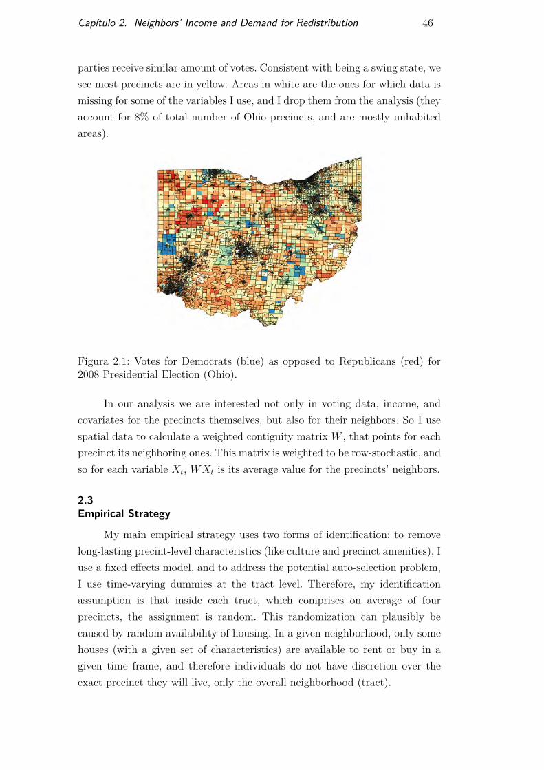
Capítulo 2. Neighbors’ Income and Demand for Redistribution 46
parties receive similar amount of votes. Consistent with being a swing state, wesee most precincts are in yellow. Areas in white are the ones for which data ismissing for some of the variables I use, and I drop them from the analysis (theyaccount for 8% of total number of Ohio precincts, and are mostly unhabitedareas).
Figura 2.1: Votes for Democrats (blue) as opposed to Republicans (red) for2008 Presidential Election (Ohio).
In our analysis we are interested not only in voting data, income, andcovariates for the precincts themselves, but also for their neighbors. So I usespatial data to calculate a weighted contiguity matrix W , that points for eachprecinct its neighboring ones. This matrix is weighted to be row-stochastic, andso for each variable Xt, WXt is its average value for the precincts’ neighbors.
2.3Empirical Strategy
My main empirical strategy uses two forms of identification: to removelong-lasting precint-level characteristics (like culture and precinct amenities), Iuse a fixed effects model, and to address the potential auto-selection problem,I use time-varying dummies at the tract level. Therefore, my identificationassumption is that inside each tract, which comprises on average of fourprecincts, the assignment is random. This randomization can plausibly becaused by random availability of housing. In a given neighborhood, only somehouses (with a given set of characteristics) are available to rent or buy in agiven time frame, and therefore individuals do not have discretion over theexact precinct they will live, only the overall neighborhood (tract).

Capítulo 2. Neighbors’ Income and Demand for Redistribution 47
The main purpose of this paper is to estimate the following equation,where W is the weighted contiguity matrix, vDt is the share of votes forDemocrats in each precinct at each period t, yt is a vector of precinct incomeat time t, and Xt and XN
t are matrices of covariates (with XN ⊂ X):
vDt = αSyt + αNWyt + αIytWyt + βXt + βNWXNt +WvDt + ut
The error u is divided in fixed precinct-level unobservables ξp, time-varying tract-level unobservable characteristics ζc,t and a time-varyingprecinct-level error εp,t, that is, up,t = ξp + ζc,t + εp,t. While I cannot ad-dress the latter, I control for the first two sources of heterogeneity using awithin regression with tract-year dummies. Therefore, our main identificationassumption is that εp,t is uncorrelated with the independent variables; thatinside a tract the choice of precinct is essentially random. As stated, the factthat there is a limited amount of residences with given characteristics availableon the housing market at any given time makes this assumption plausible. Ishow evidence consistent with it in Section 5.
We also have a variety of controls Xt, including race, education, andpopulation density for own precinct and neighbors, age, proportion of houses onmortgage, employment sector, self-employed, and proportion of foreigners. Themain measures for income I use in this paper are the proportion of habitantswith low and high income, defined as the proportion with less than 30 thousanddollars a year and more than 100 thousand dollars a year, respectively. Table1 below shows the descriptive statistics for the main variables in our empiricalexercise.
A potential issue with this data is that because of its spatial nature,the dependent variable and errors can be spatially correlated. Indeed, inFigure 2.2 below I show that this concern is valid, namely that share ofvotes for Democrats is significantly spatially correlated. Consequently, I followthe spatial econometrics literature and estimate, besides linear fixed-effectsregressions (with errors clustered at the county level to account for spatialautocorrelation), a spatial autoregressive panel model, including a spatiallag of the dependent variable (share of votes for Democrats) to account forunobserved factors that are spatially correlated (as in the estimation formulaabove). I estimate this model by Maximum Likelihood.5
5I do not use neighbors’ votes for Democrats in the linear model because it is (byconstruction) endogenous, and it would bias the results. As I will discuss in the next section,the coefficient of spatial correlation—given our controls—is actually small, which explainswhy both specifications give very similar results.

Capítulo 2. Neighbors’ Income and Demand for Redistribution 48
Tabe
la2.1:
Descriptiv
eStatist
ics.
Min
1stQua
rtile
Med
ian
Mean
3rdQua
rtile
Max
Std.
Deviatio
nYe
ar:2
004
Popu
latio
n117.0000
1009.3051
1289.9995
1602.3226
1792.9938
8839.000
010
20.533
1Area
0.0233
0.3558
1.4370
6.1135
7.1229
87.6120
10.038
4Sh
arevo
tes(D
)0.0644
0.3581
0.4620
0.4947
0.5952
1.0000
0.18
51Highincome
0.0000
0.1058
0.1798
0.2204
0.2923
0.9429
0.15
61Lo
wincome
0.0000
0.1569
0.2456
0.2718
0.3619
0.9118
0.15
41Av
gincome
9.3501
10.6392
10.8372
10.8695
11.0591
12.953
10.36
20Black
0.0000
0.0043
0.0142
0.0981
0.0584
0.9936
0.21
46Hisp
anic
0.0000
0.0056
0.0094
0.0171
0.0160
0.6070
0.03
34Fo
reign-bo
rn0.0000
0.0083
0.0183
0.0281
0.0374
0.2945
0.02
95Und
ergrad
uate
0.0000
0.0662
0.1122
0.1404
0.1984
0.5623
0.09
69Highscho
ol0.1020
0.5673
0.6458
0.6192
0.7014
0.8641
0.11
64Gradu
ate
0.0000
0.0209
0.0405
0.0597
0.0805
0.5229
0.05
63Ye
ar:2
008
Popu
latio
n83.0000
971.8124
1318.5300
1723.5085
1930.6641
10096.00
0012
98.210
3Area
0.0233
0.3558
1.3912
5.9101
6.7030
87.6120
9.85
98Sh
arevo
tes(D
)0.0978
0.3938
0.4950
0.5288
0.6230
1.0000
0.18
46Highincome
0.0000
0.0675
0.1342
0.1754
0.2404
1.0000
0.14
83Lo
wincome
0.0000
0.1756
0.2673
0.2943
0.3897
0.9816
0.16
04Av
gincome
9.1190
10.7497
10.9829
11.0002
11.2263
13.026
70.40
20Black
0.0000
0.0000
0.0173
0.1118
0.0876
1.0000
0.22
20Hisp
anic
0.0000
0.0002
0.0090
0.0231
0.0264
0.5936
0.04
41Fo
reign-bo
rn0.0000
0.0083
0.0217
0.0343
0.0473
0.4208
0.03
76Und
ergrad
uate
0.0000
0.0720
0.1250
0.1530
0.2163
0.6312
0.10
48Highscho
ol0.0282
0.5655
0.6637
0.6313
0.7267
0.9116
0.13
59Gradu
ate
0.0000
0.0264
0.0530
0.0723
0.0985
0.5131
0.06
47H
igh
inco
me
ispr
opor
tion
ofpr
ecin
ctpo
pula
tion
earn
ing
mor
eth
an10
0th
ousa
nddo
llars
aye
ar,
and
low
inco
me
the
prop
orti
onea
rnin
gle
ssth
an30
thou
sand
dolla
rspe
rye
ar.
Shar
eof
vote
sfo
rD
emoc
rats
isvo
tes
(D)
vote
s(D
)+vo
tes
(R).
The
rear
e10
,119
obse
rvat
ions
per
year
.
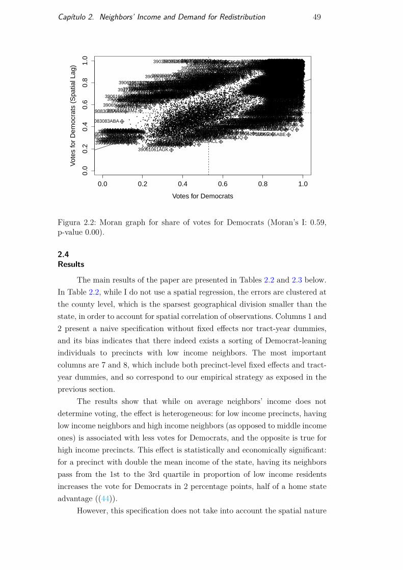
Capítulo 2. Neighbors’ Income and Demand for Redistribution 49
0.0 0.2 0.4 0.6 0.8 1.0
0.0
0.2
0.4
0.6
0.8
1.0
Votes for Democrats
Vot
es fo
r D
emoc
rats
(S
patia
l Lag
)
39001001AAF
39001001ABE
39003003ACB
39003003ABX
39003003ABQ
39003003ABP
39003003AEW39003003AEX
39003003ABZ39003003ABW
39007007AAQ
39011011AAV
39011011ABF39017017AGW
39017017ACF39017017AKE39017017AJY39017017ALH
39017017AFH39017017AKN
39017017AEE
39017017AFO
39017017AAS 39017017ADC
39017017AGE39017017AHX
39017017AFI
39019019AAC
39023023ADA
39023023ACU39023023ACT
39023023ACN
39029029ADC
39035035AMM39035035APP39035035DDY39035035DED 39035035AUH
39035035AVK
39035035AWK
39035035AWS
39035035AXL39035035AXT
39035035BBB
39035035AXY
39035035AWY39035035AVQ
39035035AZU
39035035AZH
39035035AXQ
39035035AQG
39035035AQA
39035035ANF
39035035AMO39035035AME
39035035ALS39035035ALL
39035035CDL
39035035AKZ39035035AUE
39035035CCT
39035035BQF39035035BPG
39035035CZU39035035BOA
39035035CVM
39035035AUF
39035035APX
39035035AOQ
39035035ALF
39035035CZZ
39035035AFV
39035035CDD
39035035AWU
39035035AWO39035035AWE
39035035AUJ39035035ATZ
39035035ARO39035035BQJ
39035035ARG39035035AQE
39035035APV39035035ANP
39035035AFL39035035BEW39035035BEF
39035035ANA
39035035AMV39035035AMU
39035035AMS39035035AMK
39035035AMI
39035035CQD
39035035AMQ39035035AMC
39035035ALR39035035BVN
39035035BTO
39035035BPH
39035035CTF
39035035ALW
39035035ALU39035035ALT39035035ALQ39035035ALN
39035035ALJ
39035035ALD
39035035ALB39035035AQO
39035035AVD
39035035AQS39035035AYL39035035AXJ
39035035AWN
39035035CDJ39035035BCI39035035CWB39035035BGP
39035035CSZ
39035035CSX
39035035BCS
39035035DEA39035035CSB39035035BLZ
39035035BQW
39035035ANC
39035035AZK
39035035BME
39035035BSF
39035035ATF39035035AXV
39035035BAI39035035AVF
39035035AOU
39035035BGK
39035035AON
39035035AOF39035035AOD39035035ANR39035035ANB
39035035AKX39035035AKR
39035035AKP
39035035AZS
39035035AHS39035035BNX
39035035ASF
39035035DAO39035035CNI 39035035CWI
39035035AUX39035035ATJ39035035ARV
39035035APR
39035035ANE
39035035AMG
39035035CSR
39035035CSN
39035035CQR
39035035BVQ
39035035ALH39035035AQH
39035035ARM
39035035AMZ39035035AZE
39035035CZJ
39035035AMX39035035AOS
39035035BOP39035035CQY
39035035CTB
39035035CTQ
39035035BPI
39035035BRD
39035035BNH
39035035BPL
39035035CSF
39035035ADR
39035035BQI39035035ALV
39035035BQU
39035035BRB
39035035CTO39035035BQK
39035035AXR
39035035AXP39035035AXO
39035035AXN39035035AVP39035035AVL39035035AUI39035035ATP
39035035ATH
39035035ASV
39035035AJN
39035035DEC
39035035CDM
39035035CDI
39035035CDH
39035035DAP
39035035DEE39035035DDZ39035035AVO39035035AVM
39035035AVJ39035035AVG
39035035BVM
39035035CDN
39035035BNY 39035035BNI
39035035CTP39035035AYJ39035035BSX39035035BRA
39035035BQV
39035035BOB
39035035BNK39035035BNG
39035035BNF
39035035BMR39035035BMQ 39035035AWQ39035035AWG
39035035CDC39035035CCX39035035BJV
39035035BJM
39035035ATN39035035ATL
39035035ARK39035035AQM
39035035DDX 39035035AQC39035035AQB39035035BOR39035035BPF
39035035AFK39035035AFH
39035035AFG
39035035AFB39035035CDK
39035035BTH
39035035BPJ39035035AWC
39035035BIU
39035035BPE39035035BPD39035035BOM
39035035BQE
39035035BQG
39035035BQX
39035035AXX39035035AXW
39035035AXU39035035AXS39035035AXH39035035AWZ39035035AWX39035035AWW39035035AWV39035035AWT39035035AWR39035035AWP
39035035AQD
39035035APZ
39035035AVB
39035035AUZ39035035AUT39035035AUR39035035AUG39035035AUD39035035AUB39035035ATV
39035035ATT39035035ATR39035035CTG
39035035CTD39035035ASJ
39035035ASH
39035035CNV39035035CWL
39035035BUI
39035035BTM
39035035BTI
39035035BTF39035035BSZ
39035035AFA
39035035AES 39035035BVP
39035035CQV
39035035AVI39035035ATX39035035ASR
39035035AKA
39035035AVY
39035035BIW39035035BIQ
39035035APY39035035APT
39035035APL
39035035APJ39035035DDP
39035035AOT
39035035AOR
39035035CZI39035035CZB39035035BVV
39035035ALP
39035035BRC
39035035AFU39035035AFM39035035BOV
39035035BQH
39035035ADV
39035035CTR39035035BVO
39035035ARN
39035035ARH39035035CEK
39037037ABL
39037037ABF
39037037ABD
39037037AAZ
39037037ABK
39037037ABU
39037037AAW
39037037ABS
39037037AAX
39037037ABC
39037037ABH
39037037ABJ
39037037ABV
39037037AAO
39037037AAK39037037AAC 39037037ABT
39037037ABN
39037037AAL
39037037ABX39037037ABR
39037037AAS39037037AAI
39037037AAA
39037037ABY
39037037ABP
39037037ACA39037037ABQ
39039039ABQ39039039AAA
39041041AAC39043043AEA
39043043ADZ
39049049ALO
39049049AKC
39049049AFG
39049049AIN
39049049BCW
39049049AIJ
39049049AFJ39049049AEN
39049049AEA
39049049BDV
39049049AFQ
39049049AHY
39049049AHX
39049049ADR
39049049AID
39049049ADG
39049049AHQ39049049AFK
39049049AFH
39049049ANI
39049049AED
39049049AYW39049049ACB
39049049AET
39049049AOX
39049049AGB
39049049AYQ
39049049AEM
39049049ALC
39049049AKK
39049049AYT
39049049AEH
39049049AEF
39049049BEM 39049049AEK
39049049AOS
39049049AZD39049049AXU
39049049AEE
39049049AEC
39049049ADZ
39049049AGD
39049049AGC
39049049AOV
39049049AEB
39049049BDL
39049049BCJ39049049AMF
39049049ALK
39049049AHS
39049049ADI
39049049ADY
39049049ADS
39049049AGA
39049049AMS
39049049ALP
39049049AOR
39049049ADT
39049049AKQ
39049049ABJ
39049049AJQ
39049049AIK39049049AHW39049049AZA
39049049AKE
39049049AMY
39049049AKD
39049049ABH
39049049ANK39049049ANJ39049049BDF
39049049ALS
39049049ALL39049049AAG39049049AYU
39049049AHV
39051051AAA
39051051ABC
39053053ABJ39055055ADN
39055055ACT39055055ADP
39055055ACU39055055ACQ
39055055ACR39057057ACO
39061061AGK
39061061ATW
39061061AUP
39061061ATT39061061ATD39061061ASZ39061061ASS39061061BMA
39061061BOG
39061061BGQ
39061061AYH39061061AYD
39061061BGR
39061061BMW
39061061BOC
39061061BBW39061061BAV
39061061AMO
39061061AMI
39061061BLI39061061BND
39061061BMZ
39061061BMK
39061061BBA
39061061BKM39061061BLT
39061061AZL39061061BAS
39061061BKA
39061061AYI
39061061ALX
39061061AXV
39061061ALR
39061061ALG
39061061ALF
39061061ALA
39061061BBQ
39061061BBE
39061061ATN39061061AXN
39061061BBG
39061061ATC39061061AWZ
39061061BCE
39061061BBV
39061061ASR
39061061ASL
39061061AAF
39061061ASJ
39061061ASI
39061061AQX
39061061AQR
39061061AQP39061061AQK
39061061AQG
39061061BGU
39061061BGL
39061061ASH39061061AFK
39061061BFQ
39061061ARS
39061061BFK39061061AZW
39061061AZS
39061061AMU
39061061AMK
39061061BDX
39061061AVV
39061061BPY
39061061AMF 39061061AYM39061061AZV39061061AZR39061061ASP
39061061BGP
39061061AUI
39061061BOF
39061061BKZ
39061061BNS
39061061BNZ
39061061AEE39061061BBJ
39061061BBS
39061061BCX39061061AMS39061061ASK
39061061AXG
39061061AYR
39061061AMG39061061AWU
39061061ATA
39061061ASV39061061AWT
39061061AWL
39061061AGS
39061061AFQ
39061061APM
39061061AWF
39061061ASM
39061061ASQ
39061061AUS
39061061AOX
39061061ANL
39061061BNF
39061061AQY
39061061ALU 39061061ALJ
39061061AMW
39061061ALH
39061061AGT
39061061AZB
39061061BPF39061061BPC
39061061APS39061061APK
39061061AOV
39061061AOR
39061061AUN
39061061AUE
39061061AYF
39061061BQA
39061061AQU
39061061AQQ
39061061AQI
39061061ANM
39061061AXA
39061061AGF39061061BKG
39061061AWH
39061061BIF
39061061BNV
39061061APL39061061AQM
39061061AOY
39061061AMJ39061061BNQ39061061BNO
39061061AGW
39061061AQS
39061061AQO39061061APW
39061061BNA
39061061ALI
39061061AGP
39061061BMX
39061061AXL
39061061AXC39061061AWX
39061061BHB
39061061AFH
39061061APO
39061061AOT39061061AOP
39061061BCN
39061061AUJ
39061061AXY
39061061ATX
39061061ATU
39061061ATR
39061061AQC
39061061APY
39061061APU
39061061APQ
39061061AOZ
39061061ASA
39061061AOU
39061061AOS
39061061AYX
39063063ACO
39063063ACK39063063ABC39063063AAE39063063AAO
39063063ABW
39063063ACL39063063AAG
39063063AAR39063063AAA39063063AAU 39063063AAK
39065065ABG
39065065ABJ
39065065AAF
39065065ABM
39065065AAQ
39065065AAJ 39065065ABE
39065065ABB
39065065AAM
39067067AAA39067067ABI39067067AAS3906935AAH
3906935−AAJ3906935−AAK
3906935−ABE39071071AAI
39073073AAI39073073AAK39073073AAG
39073073AAM
39073073AAJ
39073073AAE
39073073AAS
39073073AAO
39073073AAL
39073073AAB
39083083AAL39083083AAK
39083083AAN
39083083ABD
39083083ABA
39083083ABE
39085085AGQ
39085085AHT
39085085ACT39085085ACR39085085ACH
39089089AAS39091091AAG39093093AEM
39093093AIV 39093093AEI
39095095ARF39095095ACN39095095AUE
39095095ARJ
39095095ARH
39095095APV39095095APU
39095095ABJ 39095095AQG39095095AOU39095095AQM
39095095ARM
39095095AVG
39095095AUJ
39095095ASO39095095ASM
39095095AUQ39095095AVP39095095ABU
39095095ABO39095095AUP
39095095ASE
39095095ARI
39095095ASH
39095095ASG
39095095ARD
39095095AUS39095095AVI
39095095AVS
39095095AUM
39095095AUG
39095095ATZ
39095095AUF39095095AUU
39095095ARG
39095095ARE
39095095ATT
39095095AVX
39095095AFL
39095095AUK39095095ATY
39095095AUN
39095095AVO39095095ASW
39095095ASN
39095095ASJ
39095095ABG 39095095APB39095095AOX
39095095AFM
39095095ADZ
39095095AQL39095095AOV
39095095ABZ
39095095ACM39095095ANE39095095ADU39095095AFN39095095AVR
39095095AUL
39095095AUD39095095ADI
39095095ADD39095095AQN
39095095AUA39095095ATV39095095ACT
39095095ATU
39095095APA39095095AOZ39095095AOY39095095AON39095095AEN
39095095AOM
39095095ASI
39095095APZ
39095095AIX
39095095APG
39095095APJ
39095095AQW
39095095AQP
39095095AQH
39095095AQC39095095AOP
39095095AOO39095095ARK39097097AAE39097097ABQ
39097097AAU
39097097ABI39099099AQA
39099099AQD
39099099AQM39099099ABJ39099099AQE39099099AQB39099099ABT 39099099AQF
39099099AQG
39099099ASZ
39099099ARY39099099ARX
39099099ASG39099099AOR
39099099ASB
39099099ARU39099099AQU
39099099AFP
39099099AQK39099099AFS39099099AGP
39099099AGK
39099099ASL
39099099AQL39099099AQN
39099099AGS
39099099AQJ
39099099AQH
39099099APE
39099099ASQ
39099099AJG
39099099AQI
39099099ARV
39099099ASA
39099099APX
39099099AIV
39099099ASN
39099099ACK39113113APM
39113113ABQ
39113113APR
39113113ARH39113113ARG
39113113ANE39113113ANW
39113113ANU
39113113ARR
39113113AQS
39113113AQR
39113113AQM39113113AQL
39113113AQI
39113113ANT39113113ANM39113113ANK
39113113ASC
39113113ANF
39113113APZ
39113113AGF39113113ASA
39113113APL
39113113ARV
39113113ASE
39113113AEJ
39113113AQF
39113113AQA
39113113ARX
39113113ARU
39113113AEM
39113113AKY
39113113APS
39113113APP
39113113APK
39113113APJ
39113113AQO
39113113AEZ39113113ADX
39113113ASD
39113113AIT
39113113AQN
39113113ARF
39113113ARE
39113113ASB
39113113ARZ
39113113AEQ
39113113AMV
39113113ARP
39113113ALE 39113113ART39113113ARS
39113113ARQ
39113113ADZ39113113ADW39113113ADJ
39113113ARI
39113113AQK
39113113ANS
39113113ANL
39113113APF39113113AQJ
39113113ANP
39113113AVV
39113113API
39113113AQD
39113113AQC39115115AAU
39115115AAW
39115115AAQ
39115115AAA
39115115AAI39115115AAN39115115AAL
39117117AAC
39117117AAW39117117AAD
39117117AAP
39117117AAE39117117AAF
39117117AAX39117117ABH
39117117AAQ
39117117AAM
39117117AAS39119119ACX
39119119ACV
39119119ACT 39119119AAG39119119AAO
39119119ABB
39119119ACO39119119ADC39119119ACE
39119119ABT
39119119ACJ39119119ACK
39119119AAM
39119119ACM
39127127AAH
39133133AGN
39135135AAY
39141141ABK39143143AAF
39143143AAM
39143143ACQ39143143ABO39143143ABM
39143143ADE
39143143ABL
39143143ADI
39145145AAA
39151151AKO
39151151AKL
39151151ANB
39151151ABW39151151AMI
39151151AJW
39151151ALF
39151151AJU
39151151AOS
39151151AKP
39151151AKH39151151ANI
39151151ALB39151151AKQ39151151AEF
39151151AJX
39151151AIM
39153153AOC
39153153API39153153AOE
39153153AML39153153AKB39153153AQD
39153153APT
39153153APR
39153153APM
39153153AQF
39153153APD
39153153APX39153153AMJ
39153153APB39153153AOX
39153153AOQ
39153153APL39153153AVG 39153153APZ
39153153APK
39153153AOS
39153153AON
39153153AOM
39153153APC
39153153AOG
39153153AOD39153153AOR
39153153AGS 39153153AOJ
39153153AOF
39153153ATT
39153153AOB
39153153AMM
39153153AOZ
39153153ATV
39153153APA
39153153APV
39153153AOI
39153153AOO
39155155AHC
39157157AEU
39157157ACU
39157157ACR
39157157ABX
39157157ACS39157157ADJ
39157157ACT39157157ACN
39157157ADE
39157157ACP39157157ABA 39157157AAR39157157ACG
39157157ABU
39171171AAV
39171171AAP
39173173ABU
Figura 2.2: Moran graph for share of votes for Democrats (Moran’s I: 0.59,p-value 0.00).
2.4Results
The main results of the paper are presented in Tables 2.2 and 2.3 below.In Table 2.2, while I do not use a spatial regression, the errors are clustered atthe county level, which is the sparsest geographical division smaller than thestate, in order to account for spatial correlation of observations. Columns 1 and2 present a naive specification without fixed effects nor tract-year dummies,and its bias indicates that there indeed exists a sorting of Democrat-leaningindividuals to precincts with low income neighbors. The most importantcolumns are 7 and 8, which include both precinct-level fixed effects and tract-year dummies, and so correspond to our empirical strategy as exposed in theprevious section.
The results show that while on average neighbors’ income does notdetermine voting, the effect is heterogeneous: for low income precincts, havinglow income neighbors and high income neighbors (as opposed to middle incomeones) is associated with less votes for Democrats, and the opposite is true forhigh income precincts. This effect is statistically and economically significant:for a precinct with double the mean income of the state, having its neighborspass from the 1st to the 3rd quartile in proportion of low income residentsincreases the vote for Democrats in 2 percentage points, half of a home stateadvantage ((44)).
However, this specification does not take into account the spatial nature
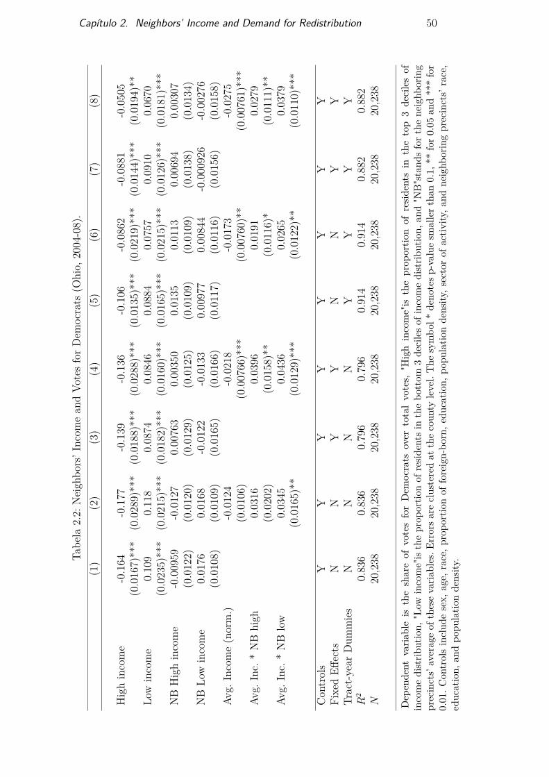
Capítulo 2. Neighbors’ Income and Demand for Redistribution 50
Tabe
la2.2:
Neigh
bors’Inc
omean
dVo
tesforDem
ocrats
(Ohio,
2004
-08).
(1)
(2)
(3)
(4)
(5)
(6)
(7)
(8)
Highincome
-0.164
-0.177
-0.139
-0.136
-0.106
-0.086
2-0.088
1-0.050
5(0.016
7)**
*(0.028
9)**
*(0.0188)**
*(0.028
8)**
*(0.013
5)**
*(0.021
9)**
*(0.014
4)**
*(0.019
4)**
Low
income
0.10
90.118
0.0874
0.0846
0.0884
0.07
570.09
100.06
70(0.023
5)**
*(0.021
5)**
*(0.0182)**
*(0.016
0)**
*(0.016
5)**
*(0.021
5)**
*(0.012
6)**
*(0.018
1)**
*NB
Highincome
-0.00959
-0.0127
0.00
763
0.00
350
0.01
350.0113
0.00
694
0.00
307
(0.012
2)(0.012
0)(0.012
9)(0.0125)
(0.010
9)(0.0109)
(0.013
8)(0.0134)
NB
Low
income
0.0176
0.01
68-0.012
2-0.013
30.00
977
0.00
844
-0.000
926
-0.002
76(0.010
8)(0.010
9)(0.016
5)(0.0166)
(0.011
7)(0.0116)
(0.015
6)(0.0158)
Avg.
Income(norm.)
-0.012
4-0.021
8-0.017
3-0.027
5(0.010
6)(0.007
66)***
(0.007
60)**
(0.007
61)***
Avg.
Inc.
*NB
high
0.03
160.0396
0.01
910.02
79(0.020
2)(0.015
8)**
(0.011
6)*
(0.011
1)**
Avg.
Inc.
*NB
low
0.03
450.04
360.02
650.03
79(0.016
5)**
(0.0129)**
*(0.012
2)**
(0.011
0)**
*
Con
trols
YY
YY
YY
YY
FixedEff
ects
NN
YY
NN
YY
Tract-year
Dum
mies
NN
NN
YY
YY
R2
0.83
60.83
60.79
60.79
60.91
40.91
40.88
20.88
2N
20,238
20,238
20,238
20,238
20,238
20,238
20,238
20,238
Dep
ende
ntvaria
bleis
theshareof
votesforDem
ocrats
over
totalvotes,
"High
income"is
theprop
ortio
nof
resid
ents
inthetop
3de
cilesof
incomedistrib
ution,
"Low
income"istheprop
ortio
nof
resid
ents
inthebo
ttom
3de
cilesof
incomedistrib
ution,
and"N
B"stand
sforthene
ighb
oring
precincts’averageof
thesevaria
bles.E
rrorsareclusteredat
thecoun
tylevel.The
symbo
l*de
notesp-valuesm
allert
han0.1,
**for0
.05an
d**
*for
0.01.C
ontrolsinclud
esex,
age,
race,p
ropo
rtionof
foreign-bo
rn,e
ducatio
n,po
pulatio
nde
nsity
,sectorof
activ
ity,a
ndne
ighb
oringprecincts’
race,
educ
ation,
andpo
pulatio
nde
nsity
.

Capítulo 2. Neighbors’ Income and Demand for Redistribution 51
of the data and how voter ideology might spread from a precinct to itsneighbors. In Table 2.3 I use spatial panel data methods to account for this.In columns 1 and 2 I use a spatial regression without fixed effects using tract-year dummies and in columns 3 and 4 a spatial fixed effects model withoutthese spatial controls. Given that the spatial models are solved by maximumlikelihood methods, which are more demanding computationally than linearprogramming problems, I could not compute the model with both fixed effectsand tract-year dummies.
Tabela 2.3: Neighbors’ Income and Votes for Democrats (Ohio, 2004-08),spatial models.
(1) (2) (3) (4)
High income -0.1156 -0.0964 -0.1795 -0.1873(0.0089)*** (0.0110)*** (0.0095)*** (0.0106)***
Low income 0.0686 0.0562 0.0697 0.0789(0.0074)*** (0.0086)*** (0.0080)*** (0.0090)***
NB High income 0.0142 0.0122 -0.0189 -0.0181(0.0141) (0.0108) (0.0158) (0.0161)
NB Low income 0.0095 0.0083 0.0346 0.0338(0.0100) (0.0100) (0.0145)** (0.0145)*
Avg. Inc (norm.) -0.0169 -0.0179(0.0037)*** (0.0041)***
Avg. Inc * NB High 0.0183 0.0342(0.0068)*** (0.0079)***
Avg. Inc * NB Low 0.0262 0.0507(0.0067)*** (0.0079)***
ρ 0.0252 0.0256 0.0204 0.0157(0.0067)*** (0.0125)** (0.0104)* (0.0105)
Controls Y Y Y YFixed Effects N N Y YTract-year Dummies Y Y N NN 20,238 20,238 20,238 20,238
Dependent variable is the share of votes for Democrats over total votes. ρ isthe spatial correlation coefficient of votes for Democrats. Errors are assumedspatially and serially correlated, following (46). The symbol * denotes p-valuesmaller than 0.1, ** for 0.05 and *** for 0.01. Controls include sex, age, race,proportion of foreign-born, education, population density, sector of activity, andneighboring precincts’ race, education, and population density. Estimated using(45).
Interestingly, the results are qualitatively and quantitatively similar tothose in Table 2.2, which indicates that the spatial nature of the data doesnot affect our results significantly when controlling for tract-year dummies.
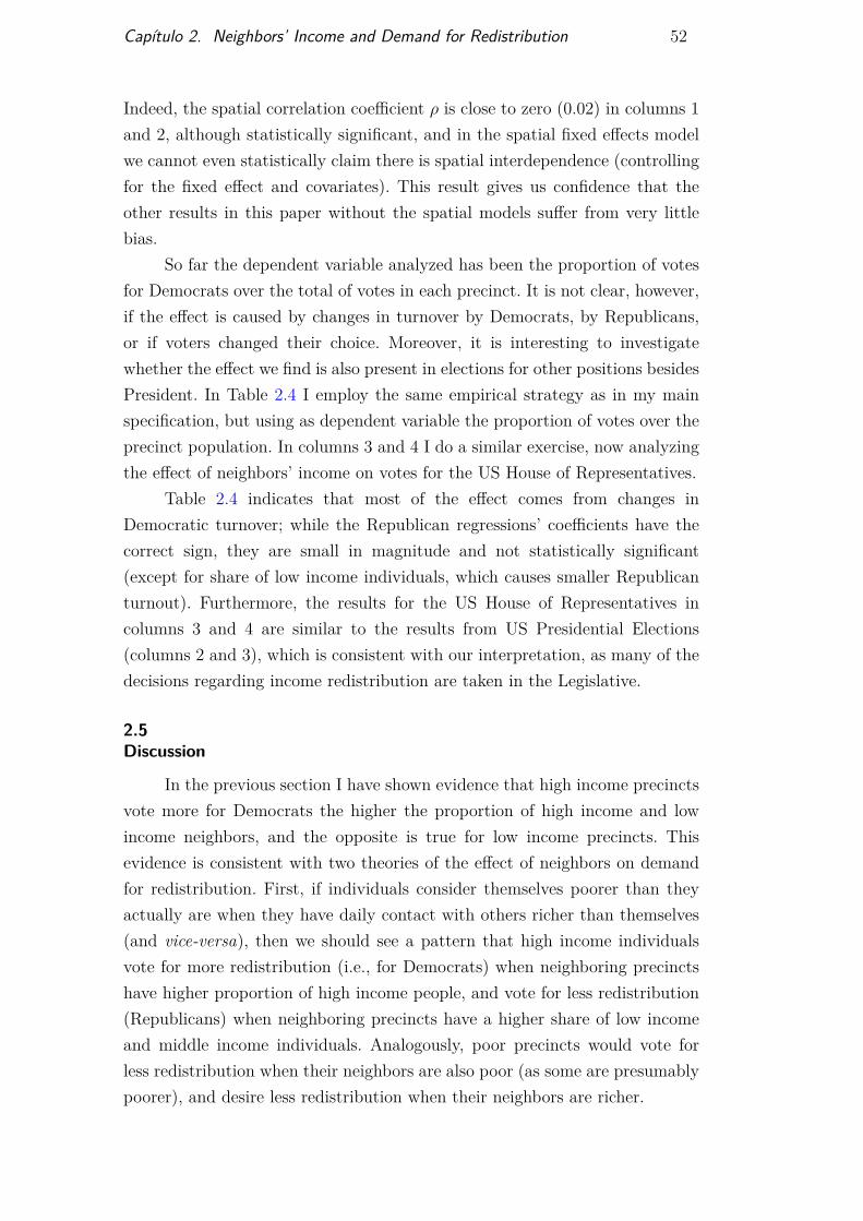
Capítulo 2. Neighbors’ Income and Demand for Redistribution 52
Indeed, the spatial correlation coefficient ρ is close to zero (0.02) in columns 1and 2, although statistically significant, and in the spatial fixed effects modelwe cannot even statistically claim there is spatial interdependence (controllingfor the fixed effect and covariates). This result gives us confidence that theother results in this paper without the spatial models suffer from very littlebias.
So far the dependent variable analyzed has been the proportion of votesfor Democrats over the total of votes in each precinct. It is not clear, however,if the effect is caused by changes in turnover by Democrats, by Republicans,or if voters changed their choice. Moreover, it is interesting to investigatewhether the effect we find is also present in elections for other positions besidesPresident. In Table 2.4 I employ the same empirical strategy as in my mainspecification, but using as dependent variable the proportion of votes over theprecinct population. In columns 3 and 4 I do a similar exercise, now analyzingthe effect of neighbors’ income on votes for the US House of Representatives.
Table 2.4 indicates that most of the effect comes from changes inDemocratic turnover; while the Republican regressions’ coefficients have thecorrect sign, they are small in magnitude and not statistically significant(except for share of low income individuals, which causes smaller Republicanturnout). Furthermore, the results for the US House of Representatives incolumns 3 and 4 are similar to the results from US Presidential Elections(columns 2 and 3), which is consistent with our interpretation, as many of thedecisions regarding income redistribution are taken in the Legislative.
2.5Discussion
In the previous section I have shown evidence that high income precinctsvote more for Democrats the higher the proportion of high income and lowincome neighbors, and the opposite is true for low income precincts. Thisevidence is consistent with two theories of the effect of neighbors on demandfor redistribution. First, if individuals consider themselves poorer than theyactually are when they have daily contact with others richer than themselves(and vice-versa), then we should see a pattern that high income individualsvote for more redistribution (i.e., for Democrats) when neighboring precinctshave higher proportion of high income people, and vote for less redistribution(Republicans) when neighboring precincts have a higher share of low incomeand middle income individuals. Analogously, poor precincts would vote forless redistribution when their neighbors are also poor (as some are presumablypoorer), and desire less redistribution when their neighbors are richer.
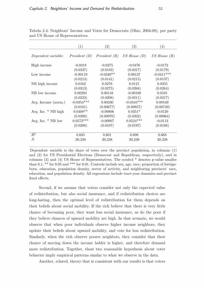
Capítulo 2. Neighbors’ Income and Demand for Redistribution 53
Tabela 2.4: Neighbors’ Income and Votes for Democrats (Ohio, 2004-08), per partyand US House of Representatives.
(1) (2) (3) (4)
Dependent variable: President (D) President (R) US House (D) US House (R)
High income -0.0318 -0.0275 -0.0476 -0.0172(0.0337) (0.0183) (0.0317) (0.0179)
Low income -0.00119 -0.0340** 0.00137 -0.0411***(0.0213) (0.0141) (0.0215) (0.0137)
NB high income 0.0162 0.0278 0.0121 0.0355(0.0313) (0.0275) (0.0268) (0.0264)
NB low income 0.00294 0.00148 -0.00100 0.0101(0.0223) (0.0208) (0.0211) (0.0217)
Avg. Income (norm.) -0.0354*** 0.00330 -0.0316*** 0.00549(0.0101) (0.00677) (0.00857) (0.00749)
Avg. Inc. * NB high 0.0408** -0.00806 0.0351* -0.0120(0.0200) (0.00970) (0.0202) (0.00964)
Avg. Inc. * NB low 0.0573*** -0.00907 0.0524*** -0.0113(0.0200) (0.0107) (0.0197) (0.0108)
R2 0.685 0.601 0.698 0.668N 20,238 20,238 20,238 20,238
Dependent variable is the share of votes over the precinct population, in columns (1)and (2) for US Presidential Elections (Democrat and Republican, respectively), and incolumns (3) and (4) US House of Representatives. The symbol * denotes p-value smallerthan 0.1, ** for 0.05 and *** for 0.01. Controls include sex, age, race, proportion of foreign-born, education, population density, sector of activity, and neighboring precincts’ race,education, and population density. All regressions include tract-year dummies and precinctfixed effects.
Second, if we assume that voters consider not only the expected valueof redistribution, but also social insurance, and if redistribution choices arelong-lasting, then the optimal level of redistribution for them depends ontheir beliefs about social mobility. If the rich believe that there is very littlechance of becoming poor, they want less social insurance, as do the poor ifthey believe chances of upward mobility are high. In that scenario, we wouldobserve that when poor individuals observe higher income neighbors, theyupdate their beliefs about upward mobility, and vote for less redistribution.Similarly, when the rich observe poorer neighbors, they consider that theirchance of moving down the income ladder is higher, and therefore demandmore redistribution. Together, these two reasonable hypothesis about voterbehavior imply empirical patterns similar to what we observe in the data.
Another, related, theory that is consistent with our results is that voters

Capítulo 2. Neighbors’ Income and Demand for Redistribution 54
might make inferences about social mobility by observing the size of the tails ofincome distribution in their neighborhood. Observing more high income andlow income residents as opposed to middle income ones updates their priorabout how unequal the society is. As in the theory above, this has differentialeffect depending on the voter’s income. A poor voter might perceive increasedinequality and social mobility as opportunity for upward mobility, and sorequest less redistribution. On the other hand, high income voters see theirwealth as less persistent, and demand more social insurance.
One plausible concern for this paper’s empirical strategy is identification.Although I employ precinct fixed effects and tract-year dummies (each tracthas on average four precincts), it is possible that individuals sort within tractand within an election cycle in such a way that more liberal high incomeindividuals prefer to live closer to low income and high income individuals,while Republican-leaning low income voters attempt to move closer to highincome and low income precincts. Even though it is not clear why such aspecific sorting pattern should occur, it could still be responsible for our results(or parts of it).
Indeed, our identification hypothesis is that within a tract, housinglocation is random. Namely, in a given time period, only a small subsetsof houses with certain characteristics (number of rooms, size, price range)are available, and therefore the buyer cannot choose exactly which blockor precinct he prefers to live, but instead can only decide on a broadergeographical area (the tract, or neighborhood).
If this is true, then any sorting (that occurs between the election cycle,so that it is not captured by the fixed effects) should be captured by our tract-year dummies, and it would not bias our results. (In terms of the estimationequation, E [εt,pyt] = 0.) If this assumption is false, however, then the resultsare potentially biased. I try to investigate this possibility in Table 2.5 below.
Table 2.5 analyzes whether neighbors’ characteristics have impact inproperty desirability, which reflects on its value. Specifically, if potential buyersprefer to buy houses near high income precincts—even within the tract—, thenthose locations should have a higher cost than comparable houses in nearbyprecincts. The data, however, shows little evidence of that. Although thecoefficient for neighbor’s proportion of high income households is marginallysignificant, the coefficient is small: a change from the 1st to 3rd quartile inneighboring precincts’ share of high income households is related to a 0.9percent increase in house value. All other coefficients are economically andstatistically insignificant.

Capítulo 2. Neighbors’ Income and Demand for Redistribution 55
Tabela 2.5: Neighbors’ Income andHouse Values (Ohio, 2004-08).
Log house value
High income 0.317(0.0443)***
Low income -0.0507(0.0602)
NB high income 0.0479(0.0265)*
NB low income 0.0100(0.0382)
Avg. Income (norm.) 0.168(0.0149)***
Avg. Inc * NB high -0.0170(0.0395)
Avg. Inc. * NB low -0.00856(0.0324)
Black -0.120(0.0513)**
Hispanic -0.206(0.142)
Bachelor degree 0.633(0.0491)***
Graduate school 0.615(0.0957)***
R2 0.919N 19,914
Dependent variable is the log of precinctmedian house value. The symbol * deno-tes p-value smaller than 0.1, ** for 0.05and *** for 0.01. Controls include sex,age, race, proportion of foreign-born, edu-cation, population density, sector of acti-vity, and neighboring precincts’ race, edu-cation, and population density.
Nonetheless, even though our evidence does not point to sorting as thedriver of our results, it must be noted that we cannot rule out that thiseffect exists and that it is the source of the stylized facts I present. Thefact that our evidence is not quasi-experimental, however, does not make ourresults uninteresting, as our analysis provides an early "big picture"view of animportant question. We welcome future evidence that would provide a causaleffect that substantiates or questions our results, although I remark that ifthe main issue is sorting and if it is believed that sorting happens quickly and
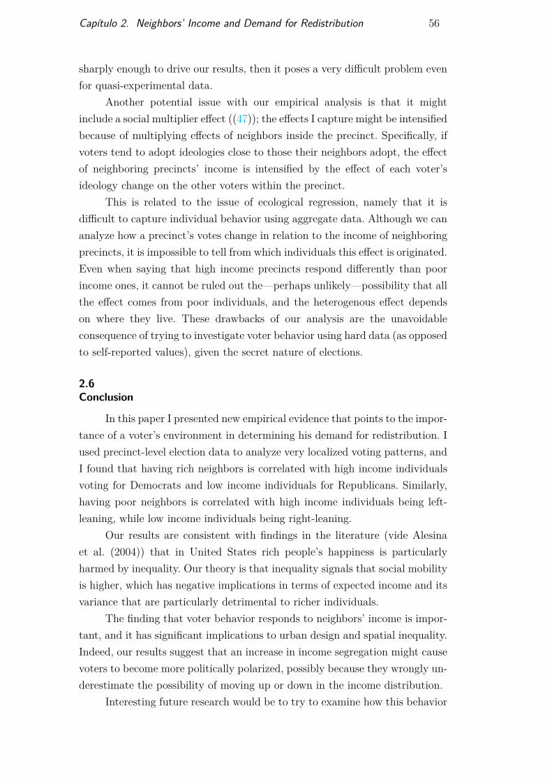
Capítulo 2. Neighbors’ Income and Demand for Redistribution 56
sharply enough to drive our results, then it poses a very difficult problem evenfor quasi-experimental data.
Another potential issue with our empirical analysis is that it mightinclude a social multiplier effect ((47)); the effects I capture might be intensifiedbecause of multiplying effects of neighbors inside the precinct. Specifically, ifvoters tend to adopt ideologies close to those their neighbors adopt, the effectof neighboring precincts’ income is intensified by the effect of each voter’sideology change on the other voters within the precinct.
This is related to the issue of ecological regression, namely that it isdifficult to capture individual behavior using aggregate data. Although we cananalyze how a precinct’s votes change in relation to the income of neighboringprecincts, it is impossible to tell from which individuals this effect is originated.Even when saying that high income precincts respond differently than poorincome ones, it cannot be ruled out the—perhaps unlikely—possibility that allthe effect comes from poor individuals, and the heterogenous effect dependson where they live. These drawbacks of our analysis are the unavoidableconsequence of trying to investigate voter behavior using hard data (as opposedto self-reported values), given the secret nature of elections.
2.6Conclusion
In this paper I presented new empirical evidence that points to the impor-tance of a voter’s environment in determining his demand for redistribution. Iused precinct-level election data to analyze very localized voting patterns, andI found that having rich neighbors is correlated with high income individualsvoting for Democrats and low income individuals for Republicans. Similarly,having poor neighbors is correlated with high income individuals being left-leaning, while low income individuals being right-leaning.
Our results are consistent with findings in the literature (vide Alesinaet al. (2004)) that in United States rich people’s happiness is particularlyharmed by inequality. Our theory is that inequality signals that social mobilityis higher, which has negative implications in terms of expected income and itsvariance that are particularly detrimental to richer individuals.
The finding that voter behavior responds to neighbors’ income is impor-tant, and it has significant implications to urban design and spatial inequality.Indeed, our results suggest that an increase in income segregation might causevoters to become more politically polarized, possibly because they wrongly un-derestimate the possibility of moving up or down in the income distribution.
Interesting future research would be to try to examine how this behavior

Capítulo 2. Neighbors’ Income and Demand for Redistribution 57
generalizes to other societies and cultures. Alesina et al. (2004) find that inEurope the effect of inequality on happiness is stronger on the poor. Would thisresult also be valid in our setting, namely is the effect of having low incomeneighbors stronger for poorer precincts than for richer precincts in Europe?Evidence to this effect would be an interesting complement to our research. Ialso hope that in the future new quasi-experimental research will be able toadd to our results.
3Party Registration and Mayoral Elections
3.1Introduction
An essential factor in promoting growth in developing countries is increa-sing the productivity of the public sector. For that purpose, it is important thatthe public bureaucracy is formed by qualified workers, and not merely used asa means of inefficient targeted redistribution by politicians towards their sup-porters. Unfortunately, political parties often use their power to appoint thepublic bureaucracy to distribute jobs among their supporters as patronage, inorder to gather assistance in elections and offer advantages to them. These ad-vantages can be significant, especially in countries where there are large rentsin working for the government, like Brazil.
In an environment with patronage, we would find that supporters of apolitical party would receive large economic benefits, in the form of offers ofwork in the public sector and higher wages from government, when that partyassumes office. This should be especially true for formal supporters of the party,in particular registered members. Additionally, since it is common for partiesto demand contributions from affiliates, giving them public jobs is an indirectway of using public funds to finance their campaigns.
In this paper we investigate the presence of patronage in municipalitiesin the Northeast of Brazil, after the 2008 mayoral elections. We empiricallyestimate the causal effect of a party winning a mayoral election on theproportion of its affiliates working for the government in the following year, aswell as their wage accrued from government. If patronage is big, then a party’svictory would have significant effect on economic outcomes of its supporters, inparticular the registered members of these parties. We also investigate whethera party winning a municipal election affects the number of affiliations to thatparty in the upcoming years, as a way for individuals to signal their supportfor that party, possibly obtaining rents from this political connection.
By analyzing this second issue, our research is also related to the questionof why voters register to political parties. One possible answer to this questionis that voters register to political parties in order to signal their support for

Capítulo 3. Party Registration and Mayoral Elections 59
that party, hoping to receive economic benefits in return. In actuality, as weargue in Section 3, most political affiliations in Brazilian municipalities aremotivated by plans of candidacy.
Our data comprises of all the registered members of political parties forall years from 1994 to 2014, and socioeconomic data for all formal employeesof firms or government, for the years 2008 and 2009, in the Northeast of Brazil.From the merged dataset we gather the affiliated member’s wage accruedfrom government and the sector of employment. The Brazilian Northeast isa particularly suitable region to analyze because anecdotal evidence points toit as the most corrupt and clientelistic region in the country.
In our empirical strategy, we obtain plausibly causal estimates of theeffect of a party’s victory on the probability of a registered member working inthe government and his wage accrued from the public sector by employing aRegression in Discontinuity (RD) design, comparing elections where the marginof victory or defeat was small. If city and party characteristics are continuousin the proportion of votes received by the party, and if candidates and voterscannot precisely control the amount of votes that a party receives, then theRD design can identify the (causal) treatment effect around the cutoff ((48)).
In both empirical exercises, we do not find consistent evidence that beingaffiliated to a political party has any positive economic value to individuals(patronage). Members of a political party do not have any higher chance ofworking for the government after the election, nor do public employees receiveany higher wage when a politician of their party or coalition wins municipalelections. Moreover, our results indicate that voters do not register to politicalparties seeking to show support; a party that narrowly wins an election is notany more likely to receive registrations than a party that narrowly loses it.
Our paper contributes to the debate on patronage, and more broadly tothe literature on inefficiencies deriving from targeted redistribution, emphasi-zed by (53) and, more recently, (54). Since in our setting the possible objects ofpatronage (political affiliates) account for almost 5 percent of the total popu-lation, the existence of targeted redistribution would cause these inefficienciesto be severe.
In that literature, (55) analyze the reverse of our research question,asking whether control of patronage increases a party’s chance of winningelections, using the implementation of civil service reform in United States.More recently, (56) provides evidence on the existence of patronage by showingthat the number of employees is higher for elected chief executives than forbureaucrats, and that this difference is higher in election years and where thereis a larger public-private wage differential.
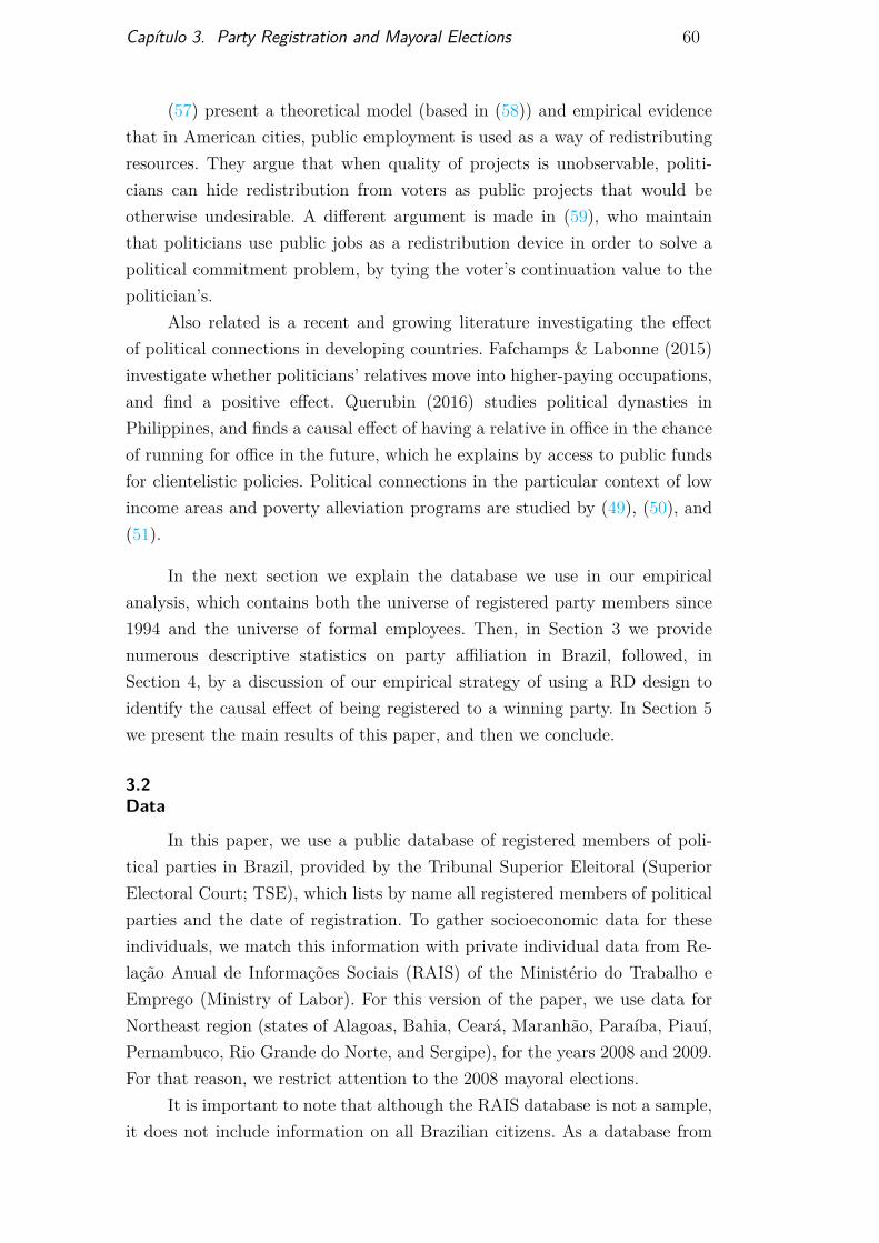
Capítulo 3. Party Registration and Mayoral Elections 60
(57) present a theoretical model (based in (58)) and empirical evidencethat in American cities, public employment is used as a way of redistributingresources. They argue that when quality of projects is unobservable, politi-cians can hide redistribution from voters as public projects that would beotherwise undesirable. A different argument is made in (59), who maintainthat politicians use public jobs as a redistribution device in order to solve apolitical commitment problem, by tying the voter’s continuation value to thepolitician’s.
Also related is a recent and growing literature investigating the effectof political connections in developing countries. Fafchamps & Labonne (2015)investigate whether politicians’ relatives move into higher-paying occupations,and find a positive effect. Querubin (2016) studies political dynasties inPhilippines, and finds a causal effect of having a relative in office in the chanceof running for office in the future, which he explains by access to public fundsfor clientelistic policies. Political connections in the particular context of lowincome areas and poverty alleviation programs are studied by (49), (50), and(51).
In the next section we explain the database we use in our empiricalanalysis, which contains both the universe of registered party members since1994 and the universe of formal employees. Then, in Section 3 we providenumerous descriptive statistics on party affiliation in Brazil, followed, inSection 4, by a discussion of our empirical strategy of using a RD design toidentify the causal effect of being registered to a winning party. In Section 5we present the main results of this paper, and then we conclude.
3.2Data
In this paper, we use a public database of registered members of poli-tical parties in Brazil, provided by the Tribunal Superior Eleitoral (SuperiorElectoral Court; TSE), which lists by name all registered members of politicalparties and the date of registration. To gather socioeconomic data for theseindividuals, we match this information with private individual data from Re-lação Anual de Informações Sociais (RAIS) of the Ministério do Trabalho eEmprego (Ministry of Labor). For this version of the paper, we use data forNortheast region (states of Alagoas, Bahia, Ceará, Maranhão, Paraíba, Piauí,Pernambuco, Rio Grande do Norte, and Sergipe), for the years 2008 and 2009.For that reason, we restrict attention to the 2008 mayoral elections.
It is important to note that although the RAIS database is not a sample,it does not include information on all Brazilian citizens. As a database from
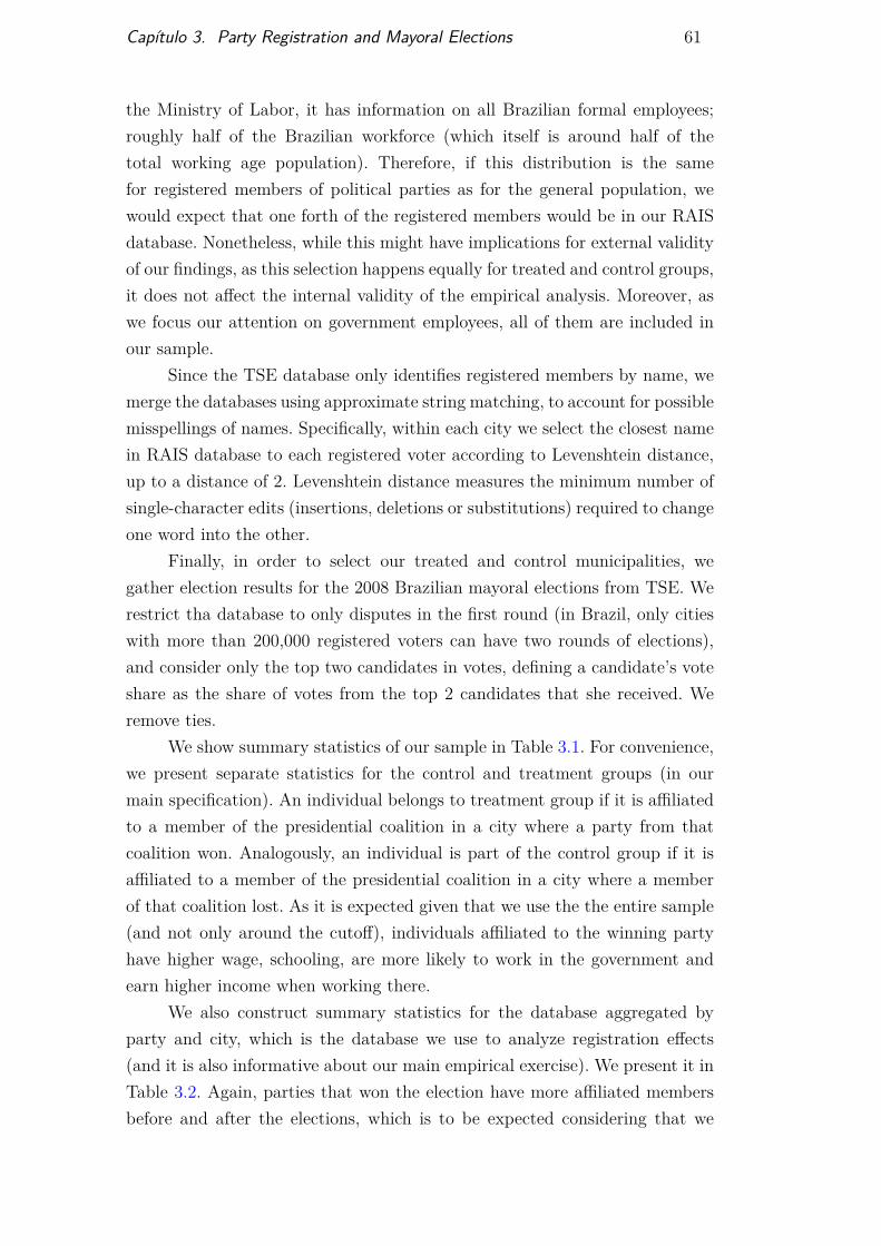
Capítulo 3. Party Registration and Mayoral Elections 61
the Ministry of Labor, it has information on all Brazilian formal employees;roughly half of the Brazilian workforce (which itself is around half of thetotal working age population). Therefore, if this distribution is the samefor registered members of political parties as for the general population, wewould expect that one forth of the registered members would be in our RAISdatabase. Nonetheless, while this might have implications for external validityof our findings, as this selection happens equally for treated and control groups,it does not affect the internal validity of the empirical analysis. Moreover, aswe focus our attention on government employees, all of them are included inour sample.
Since the TSE database only identifies registered members by name, wemerge the databases using approximate string matching, to account for possiblemisspellings of names. Specifically, within each city we select the closest namein RAIS database to each registered voter according to Levenshtein distance,up to a distance of 2. Levenshtein distance measures the minimum number ofsingle-character edits (insertions, deletions or substitutions) required to changeone word into the other.
Finally, in order to select our treated and control municipalities, wegather election results for the 2008 Brazilian mayoral elections from TSE. Werestrict tha database to only disputes in the first round (in Brazil, only citieswith more than 200,000 registered voters can have two rounds of elections),and consider only the top two candidates in votes, defining a candidate’s voteshare as the share of votes from the top 2 candidates that she received. Weremove ties.
We show summary statistics of our sample in Table 3.1. For convenience,we present separate statistics for the control and treatment groups (in ourmain specification). An individual belongs to treatment group if it is affiliatedto a member of the presidential coalition in a city where a party from thatcoalition won. Analogously, an individual is part of the control group if it isaffiliated to a member of the presidential coalition in a city where a memberof that coalition lost. As it is expected given that we use the the entire sample(and not only around the cutoff), individuals affiliated to the winning partyhave higher wage, schooling, are more likely to work in the government andearn higher income when working there.
We also construct summary statistics for the database aggregated byparty and city, which is the database we use to analyze registration effects(and it is also informative about our main empirical exercise). We present it inTable 3.2. Again, parties that won the election have more affiliated membersbefore and after the elections, which is to be expected considering that we

Capítulo 3. Party Registration and Mayoral Elections 62
Tabela 3.1: Summary statistics (full sample), separated by treatment and control (registered toa member of presidential coalition, where it won—resp. lost—the election).
Affiliated to losing party (any vote share)N Mean SD Median Min Max
Affiliation date 29031 2001.63 4.84 2003.00 1989 2007.00Wages from government (2009) 29031 668.23 1360.39 462.47 0 67022.40Male 25956 0.59 0.49 1.00 0 1.00Schooling 25956 6.23 2.01 7.00 1 11.00Age 25956 39.37 10.50 38.00 11 98.00Nominal average wage (2009) 29031 775.22 1010.07 558.00 0 44319.28Works in government (2009) 29031 0.57 0.49 1.00 0 1.00Income from city government (2009) 29031 497.77 907.00 460.83 0 37475.10
Affiliated to winning party (any vote share)N Mean SD Median Min Max
Affiliation date 32444 2001.94 4.91 2003.00 1989 2007.00Wages from government (2009) 32444 800.95 1510.96 493.30 0 42858.33Male 29365 0.59 0.49 1.00 0 1.00Schooling 29365 6.27 2.02 7.00 1 11.00Age 29365 39.49 10.70 39.00 12 108.00Nominal average wage (2009) 32444 862.42 1251.31 580.70 0 51816.30Works in government (2009) 32444 0.63 0.48 1.00 0 1.00Income from city government (2009) 32444 635.51 1229.11 465.13 0 42858.33
calculate the summary statistics using the entire database.
3.3Party Affiliation in Brazil
In this section, we present numerous stylized facts about party affiliationin Brazil, to better comprehend how and why party members differ from therest of population, and how this might affect the political process. Specifically,we compare socioeconomic characteristics between party affiliates (who areformal employees) and the rest of Brazilian formal employees, we provide thetrends of party affiliation in Brazil, and we analyze how party members thatare plausibly planning on running for elections differ from the other partyaffiliates.
At the time of 2008 Municipal Elections, there were 10,898,236 partyaffiliates in Brazil. (There were 191.8 million habitants in the country). Figure3.1 displays the number of affiliates of each of the largest 9 parties (in2012), at 2000, 2004, 2008, and 2012 Municipal Elections. Party affiliationhas increased markedly with the deepening of Brazilian democracy, especiallyin more progressive parties, like PT and PSB, both of which more than tripledtheir number of affiliates in this period. (This might also be related to PTholding the Brazilian Presidency for most of that period.)
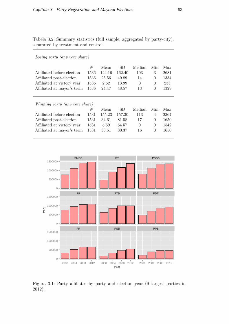
Capítulo 3. Party Registration and Mayoral Elections 63
Tabela 3.2: Summary statistics (full sample, aggregated by party-city),separated by treatment and control.
Losing party (any vote share)
N Mean SD Median Min MaxAffiliated before election 1536 144.16 162.40 103 3 2681Affiliated post-election 1536 25.56 49.89 14 0 1334Affiliated at victory year 1536 2.62 13.99 0 0 233Affiliated at mayor’s term 1536 24.47 48.57 13 0 1329
Winning party (any vote share)N Mean SD Median Min Max
Affiliated before election 1531 155.23 157.30 113 4 2367Affiliated post-election 1531 34.61 81.58 17 0 1650Affiliated at victory year 1531 5.59 54.57 0 0 1542Affiliated at mayor’s term 1531 33.51 80.37 16 0 1650
PMDB PT PSDB
PP PTB PDT
PR PSB PPS
0
500000
1000000
1500000
0
500000
1000000
1500000
0
500000
1000000
1500000
2000 2004 2008 2012 2000 2004 2008 2012 2000 2004 2008 2012year
freq
Figura 3.1: Party affiliates by party and election year (9 largest parties in2012).
Capítulo 3. Party Registration and Mayoral Elections 64
Notwithstanding the growth of parties in the presidential (left-leaning)coalition during the 2000s in Brazil, Figure 3.2 indicates that a large partof the affiliation decision is motivated by local politics; plausibly by plansof candidacy. Indeed, party registrations spike strikingly the year beforemunicipal elections. In particular, registrations for parties in the presidentialcoalition the year before 2008 Municipal Elections were 5 times higher thanthe year before that (and 2 times higher than the year after it). This factindicates that citizens register in political parties as a way to support (or runin) a municipal election—mayoral or legislative.
Oppostion Coalition Presidencial Coalition
0
200,000
400,000
600,000
1992 1996 2000 2004 2008 2012 1992 1996 2000 2004 2008 2012Year
freq
Figura 3.2: Party registrations for parties in presidential and oppositioncoalitions, per year.
Even within the year before the elections, registrations tend to concen-trate on the last weeks before the registration deadline for running in the nextyear elections. Since this deadline should be irrelevant for those not seekingcandidacy, this indicates that a large proportion of a party’s affiliations are bypeople planning on running for (mostly municipal) office. Figure 3.3 documentsthat fact.1 In Table 3.3 we compare socioeconomic characteristics between af-filiates before and after the registration limit. We argue that this accountsfor differences between registered members that intend to run in municipalelections, and those that do not.
1The plot uses monthly data for clarity, but we have daily data on registrations, and itconfirms our hypothesis. (Namely, October registrations are almost entirely concentrated inthe days before the candidacy deadline.)
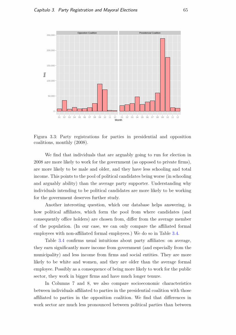
Capítulo 3. Party Registration and Mayoral Elections 65
Oppostion Coalition Presidencial Coalition
0
50,000
100,000
150,000
200,000
250,000
01 02 03 04 05 06 07 08 09 10 11 12 01 02 03 04 05 06 07 08 09 10 11 12Month
freq
Figura 3.3: Party registrations for parties in presidential and oppositioncoalitions, monthly (2008).
We find that individuals that are arguably going to run for election in2008 are more likely to work for the government (as opposed to private firms),are more likely to be male and older, and they have less schooling and totalincome. This points to the pool of political candidates being worse (in schoolingand arguably ability) than the average party supporter. Understanding whyindividuals intending to be political candidates are more likely to be workingfor the government deserves further study.
Another interesting question, which our database helps answering, ishow political affiliates, which form the pool from where candidates (andconsequently office holders) are chosen from, differ from the average memberof the population. (In our case, we can only compare the affiliated formalemployees with non-affiliated formal employees.) We do so in Table 3.4.
Table 3.4 confirms usual intuitions about party affiliates: on average,they earn significantly more income from government (and especially from themunicipality) and less income from firms and social entities. They are morelikely to be white and women, and they are older than the average formalemployee. Possibly as a consequence of being more likely to work for the publicsector, they work in bigger firms and have much longer tenure.
In Columns 7 and 8, we also compare socioeconomic characteristicsbetween individuals affiliated to parties in the presidential coalition with thoseaffiliated to parties in the opposition coalition. We find that differences inwork sector are much less pronounced between political parties than between
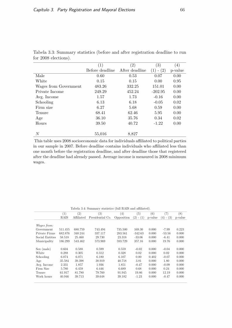
Capítulo 3. Party Registration and Mayoral Elections 66
Tabela 3.3: Summary statistics (before and after registration deadline to runfor 2008 elections).
(1) (2) (3) (4)Before deadline After deadline (1) - (2) p-value
Male 0.60 0.53 0.07 0.00White 0.15 0.15 0.00 0.95Wages from Government 483.26 332.25 151.01 0.00Private Income 249.29 452.24 -202.95 0.00Avg. Income 1.57 1.73 -0.16 0.00Schooling 6.13 6.18 -0.05 0.02Firm size 6.27 5.68 0.59 0.00Tenure 68.41 62.46 5.95 0.00Age 36.10 35.76 0.34 0.02Hours 39.50 40.72 -1.22 0.00
N 55,016 8,827This table uses 2008 socioeconomic data for individuals affiliated to political partiesin our sample in 2007. Before deadline contains individuals who affiliated less thanone month before the registration deadline, and after deadline those that registeredafter the deadline had already passed. Average income is measured in 2008 minimumwages.
Tabela 3.4: Summary statistics (full RAIS and affiliated).(1) (2) (3) (4) (5) (6) (7) (8)
RAIS Affiliated Presidential Co. Opposition (2) - (1) p-value (4) - (3) p-value
Wages from:Government 511.455 680.759 743.494 735.500 169.30 0.000 -7.99 0.223Private Firms 682.876 340.244 337.117 283.561 -342.63 0.000 -53.56 0.000Social Entities 58.518 25.460 29.730 23.318 -33.06 0.000 -6.41 0.000Municipality 186.299 543.462 573.969 593.729 357.16 0.000 19.76 0.000
Sex (male) 0.604 0.588 0.599 0.559 -0.02 0.000 -0.04 0.000White 0.288 0.305 0.312 0.328 0.02 0.000 0.02 0.000Schooling 6.074 6.071 6.180 6.107 0.00 0.402 -0.07 0.000Age 35.584 39.398 38.919 40.718 3.81 0.000 1.80 0.000Avg. Income 2.331 1.857 1.936 1.851 -0.47 0.000 -0.09 0.000Firm Size 5.780 6.459 6.446 6.689 0.68 0.000 0.24 0.000Tenure 61.917 81.780 79.760 91.945 19.86 0.000 12.19 0.000Work hours 40.946 39.713 39.648 39.182 -1.23 0.000 -0.47 0.000
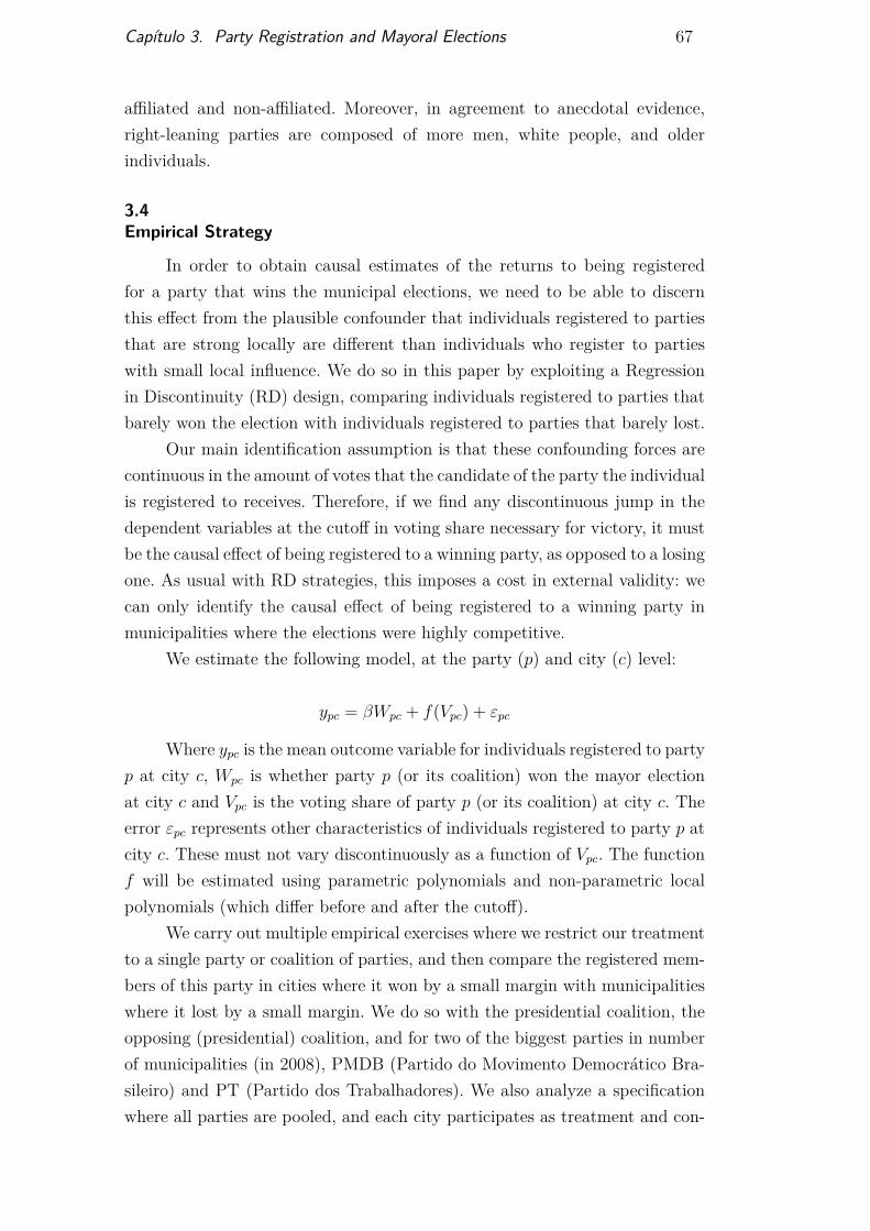
Capítulo 3. Party Registration and Mayoral Elections 67
affiliated and non-affiliated. Moreover, in agreement to anecdotal evidence,right-leaning parties are composed of more men, white people, and olderindividuals.
3.4Empirical Strategy
In order to obtain causal estimates of the returns to being registeredfor a party that wins the municipal elections, we need to be able to discernthis effect from the plausible confounder that individuals registered to partiesthat are strong locally are different than individuals who register to partieswith small local influence. We do so in this paper by exploiting a Regressionin Discontinuity (RD) design, comparing individuals registered to parties thatbarely won the election with individuals registered to parties that barely lost.
Our main identification assumption is that these confounding forces arecontinuous in the amount of votes that the candidate of the party the individualis registered to receives. Therefore, if we find any discontinuous jump in thedependent variables at the cutoff in voting share necessary for victory, it mustbe the causal effect of being registered to a winning party, as opposed to a losingone. As usual with RD strategies, this imposes a cost in external validity: wecan only identify the causal effect of being registered to a winning party inmunicipalities where the elections were highly competitive.
We estimate the following model, at the party (p) and city (c) level:
ypc = βWpc + f(Vpc) + εpc
Where ypc is the mean outcome variable for individuals registered to partyp at city c, Wpc is whether party p (or its coalition) won the mayor electionat city c and Vpc is the voting share of party p (or its coalition) at city c. Theerror εpc represents other characteristics of individuals registered to party p atcity c. These must not vary discontinuously as a function of Vpc. The functionf will be estimated using parametric polynomials and non-parametric localpolynomials (which differ before and after the cutoff).
We carry out multiple empirical exercises where we restrict our treatmentto a single party or coalition of parties, and then compare the registered mem-bers of this party in cities where it won by a small margin with municipalitieswhere it lost by a small margin. We do so with the presidential coalition, theopposing (presidential) coalition, and for two of the biggest parties in numberof municipalities (in 2008), PMDB (Partido do Movimento Democrático Bra-sileiro) and PT (Partido dos Trabalhadores). We also analyze a specificationwhere all parties are pooled, and each city participates as treatment and con-
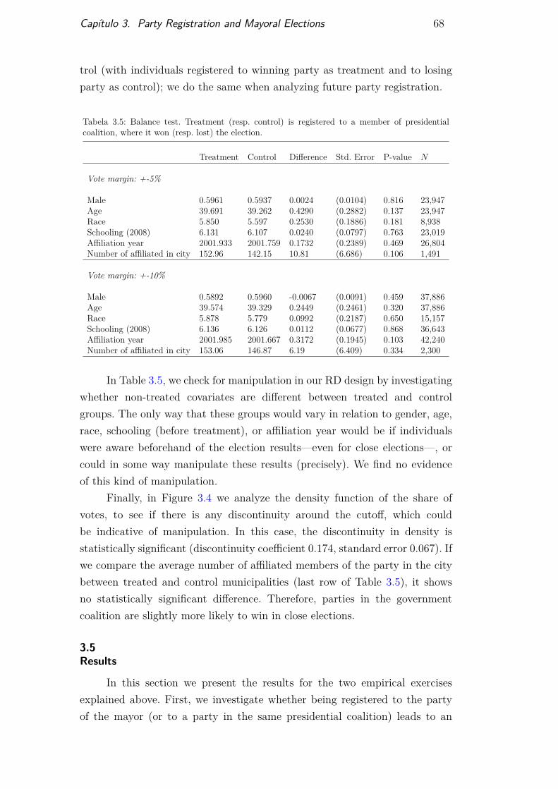
Capítulo 3. Party Registration and Mayoral Elections 68
trol (with individuals registered to winning party as treatment and to losingparty as control); we do the same when analyzing future party registration.
Tabela 3.5: Balance test. Treatment (resp. control) is registered to a member of presidentialcoalition, where it won (resp. lost) the election.
Treatment Control Difference Std. Error P-value N
Vote margin: +-5%
Male 0.5961 0.5937 0.0024 (0.0104) 0.816 23,947Age 39.691 39.262 0.4290 (0.2882) 0.137 23,947Race 5.850 5.597 0.2530 (0.1886) 0.181 8,938Schooling (2008) 6.131 6.107 0.0240 (0.0797) 0.763 23,019Affiliation year 2001.933 2001.759 0.1732 (0.2389) 0.469 26,804Number of affiliated in city 152.96 142.15 10.81 (6.686) 0.106 1,491
Vote margin: +-10%
Male 0.5892 0.5960 -0.0067 (0.0091) 0.459 37,886Age 39.574 39.329 0.2449 (0.2461) 0.320 37,886Race 5.878 5.779 0.0992 (0.2187) 0.650 15,157Schooling (2008) 6.136 6.126 0.0112 (0.0677) 0.868 36,643Affiliation year 2001.985 2001.667 0.3172 (0.1945) 0.103 42,240Number of affiliated in city 153.06 146.87 6.19 (6.409) 0.334 2,300
In Table 3.5, we check for manipulation in our RD design by investigatingwhether non-treated covariates are different between treated and controlgroups. The only way that these groups would vary in relation to gender, age,race, schooling (before treatment), or affiliation year would be if individualswere aware beforehand of the election results—even for close elections—, orcould in some way manipulate these results (precisely). We find no evidenceof this kind of manipulation.
Finally, in Figure 3.4 we analyze the density function of the share ofvotes, to see if there is any discontinuity around the cutoff, which couldbe indicative of manipulation. In this case, the discontinuity in density isstatistically significant (discontinuity coefficient 0.174, standard error 0.067). Ifwe compare the average number of affiliated members of the party in the citybetween treated and control municipalities (last row of Table 3.5), it showsno statistically significant difference. Therefore, parties in the governmentcoalition are slightly more likely to win in close elections.
3.5Results
In this section we present the results for the two empirical exercisesexplained above. First, we investigate whether being registered to the partyof the mayor (or to a party in the same presidential coalition) leads to an

Capítulo 3. Party Registration and Mayoral Elections 69
−0.2 −0.1 0.0 0.1 0.2
01
23
45
6
Share of votes
Den
sity
Figura 3.4: Estimated density function around the cutoff (McCrary test).
increased probability of being employed in the public sector or to higher wagesfor those already employed. We then study whether a party winning a mayoralelection increases the number of registrations for that party in the followingyears, plausibly as a way to signal political support and access economic gainsof political connections.
3.5.1Government Wages
In this section we investigate whether being affiliated to a party connectedto the mayor provides political connections that might help the individual enterthe bureaucracy and rise in it. We do that by comparing the average wageaccrued from and proportion that works in the government between individualsaffiliated to the party which won the election and those affiliated to the partywhich lost the election, in close races.
Before we carry out our RD design, we plot local polynomial regressionsof the log of the income accrued from the government (Figure 3.5) and theprobability of working in the government (Figure 3.6) on the proportion ofvotes for a party in the presidential coalition, where the sample is composedof individuals registered to parties in that coalition.
Neither plot shows strong evidence of a discontinuity at the victory th-reshold. We apply our main empirical specification in Table 3.6, where we esti-mate the treatment effect of being affiliated to a party in the 2006 presidential

Capítulo 3. Party Registration and Mayoral Elections 70
−0.4 −0.2 0.0 0.2 0.4
6.0
6.1
6.2
6.3
6.4
6.5
Proportion of votes for party in presidential coalition.
Wag
es a
ccru
ed fr
om g
over
nmen
t (lo
g).
Figura 3.5: Effect of mayoral victory on wages accrued from government, forindividuals registered to parties in the presidential coalition.
−0.4 −0.2 0.0 0.2 0.4
0.4
0.5
0.6
0.7
0.8
Proportion of votes for party in presidential coalition.
% e
mpl
oyed
in g
over
nmen
t.
Figura 3.6: Effect of mayoral victory on percent working for the government,for individuals registered to parties in the presidential coalition.

Capítulo 3. Party Registration and Mayoral Elections 71
coalition, when a party of that coalition wins the mayoral election, controllingfor vote share with parametric and non-parametric (local polynomial) functi-ons.2 Except for a few particular specifications, most of the coefficients cannotbe statistically discerned from zero.
Columns 1 to 6 apply parametric functions of the vote share, using onlycities where the margin of victory in the mayoral elections was less than tenand five percent, respectively. Then, in columns 7 and 8 we use nonparametriclocal linear and local quadratic function, using the entire sample. The resultsare similar in both exercises.
The fact that members of the presidential coalition are not necessarilyallied at the municipal level might introduce measurement error that wouldbias our results towards zero, attenuating the treatment effect and increasingthe variance of the estimative. Therefore, in Table 3.7 we estimate our RDdesign for two specific parties, PMDB (Partido do Movimento DemocráticoBrasileiro) and PT (Partido dos Trabalhadores). We choose these parties asthey are among the biggest in number of municipalities they controlled in 2008.
Consistently with our previous results, only in particular specificationsare the coefficients statistically significant, and they are not stable betweendifferent strategies. These results support our conclusion that there is weakevidence of any effect of being affiliated to a political party on the probabilityof working for the government in the future, or receiving higher earnings whenalready working for it.
Finally, Table 3.8 presents the results for the regression with all partiespooled. In this case, every city is both in the control group and the treatmentgroup, but with different individuals in each (we take the average value of eachgroup). In this specification, as a check of robustness, we also look at the wagesaccrued from private firms and restrict government income to wages receivedfrom the prefecture. In both cases we still find no results.
3.5.2Party Registration
If we believe that being affiliated to a political party can bring connec-tions that have economic value, then plausibly when a party wins the mayo-ral election, these connections become more valuable, and we would expectmore people to want to register to these parties. In this section we investigatewhether this happens for our sample of Northeastern Brazilian cities for the2008 mayoral election.
2(52), for example, recommend the use of non-parametric specifications as a complement,rather than substitute, of parametric forms.
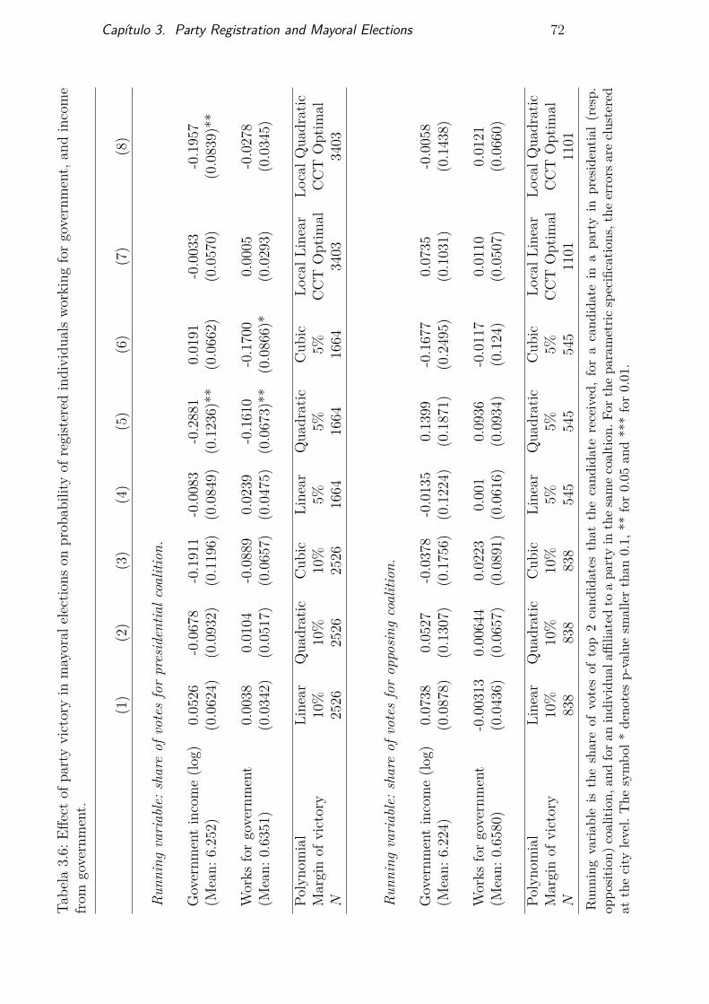
Capítulo 3. Party Registration and Mayoral Elections 72
Tabe
la3.6:
Effecto
fparty
victoryin
mayoral
electio
nson
prob
ability
ofregistered
individu
alsw
orking
forg
overnm
ent,an
dincome
from
government.
(1)
(2)
(3)
(4)
(5)
(6)
(7)
(8)
R unn
ingvariable:s
hare
ofvotesforpresiden
tialc
oalition.
Governm
entincome(lo
g)0.05
26-0.067
8-0.191
1-0.008
3-0.288
10.01
91-0.003
3-0.195
7(M
ean:
6.25
2)(0.062
4)(0.093
2)(0.119
6)(0.084
9)(0.123
6)**
(0.066
2)(0.057
0)(0.083
9)**
Works
forgovernment
0.00
380.01
04-0.088
90.02
39-0.161
0-0.170
00.00
05-0.027
8(M
ean:
0.63
51)
(0.034
2)(0.051
7)(0.065
7)(0.047
5)(0.067
3)**
(0.086
6)*
(0.029
3)(0.034
5)
P olyno
mial
Line
arQua
dratic
Cub
icLine
arQua
dratic
Cub
icLo
calL
inear
LocalQ
uadratic
Marginof
victory
10%
10%
10%
5%5%
5%CCT
Optim
alCCT
Optim
alN
2526
2526
2526
1664
1664
1664
3403
3403
R unn
ingvariable:s
hare
ofvotesforop
posing
coalition
.
Governm
entincome(lo
g)0.07
380.0527
-0.037
8-0.013
50.13
99-0.167
70.0735
-0.005
8(M
ean:
6.22
4)(0.087
8)(0.130
7)(0.175
6)(0.122
4)(0.187
1)(0.249
5)(0.103
1)(0.143
8)
Works
forgovernment
-0.003
130.00
644
0.02
230.00
10.09
36-0.011
70.01
100.01
21(M
ean:
0.65
80)
(0.043
6)(0.065
7)(0.089
1)(0.061
6)(0.093
4)(0.124
)(0.050
7)(0.066
0)
Polyno
mial
Line
arQua
dratic
Cub
icLine
arQua
dratic
Cub
icLo
calL
inear
LocalQ
uadratic
Marginof
victory
10%
10%
10%
5%5%
5%CCT
Optim
alCCT
Optim
alN
838
838
838
545
545
545
1101
1101
Run
ning
varia
bleis
theshareof
votesof
top2cand
idates
that
thecand
idatereceived
,foracand
idatein
apa
rtyin
presidentia
l(resp.
oppo
sition)
coalition
,and
fora
nindividu
alaffi
liatedto
apa
rtyin
thesamecoaltio
n.Fo
rthe
parametric
specificatio
ns,the
errors
areclustered
atthecity
level.The
symbo
l*de
notesp-valuesm
allerthan
0.1,
**for0.05
and***for0.01.
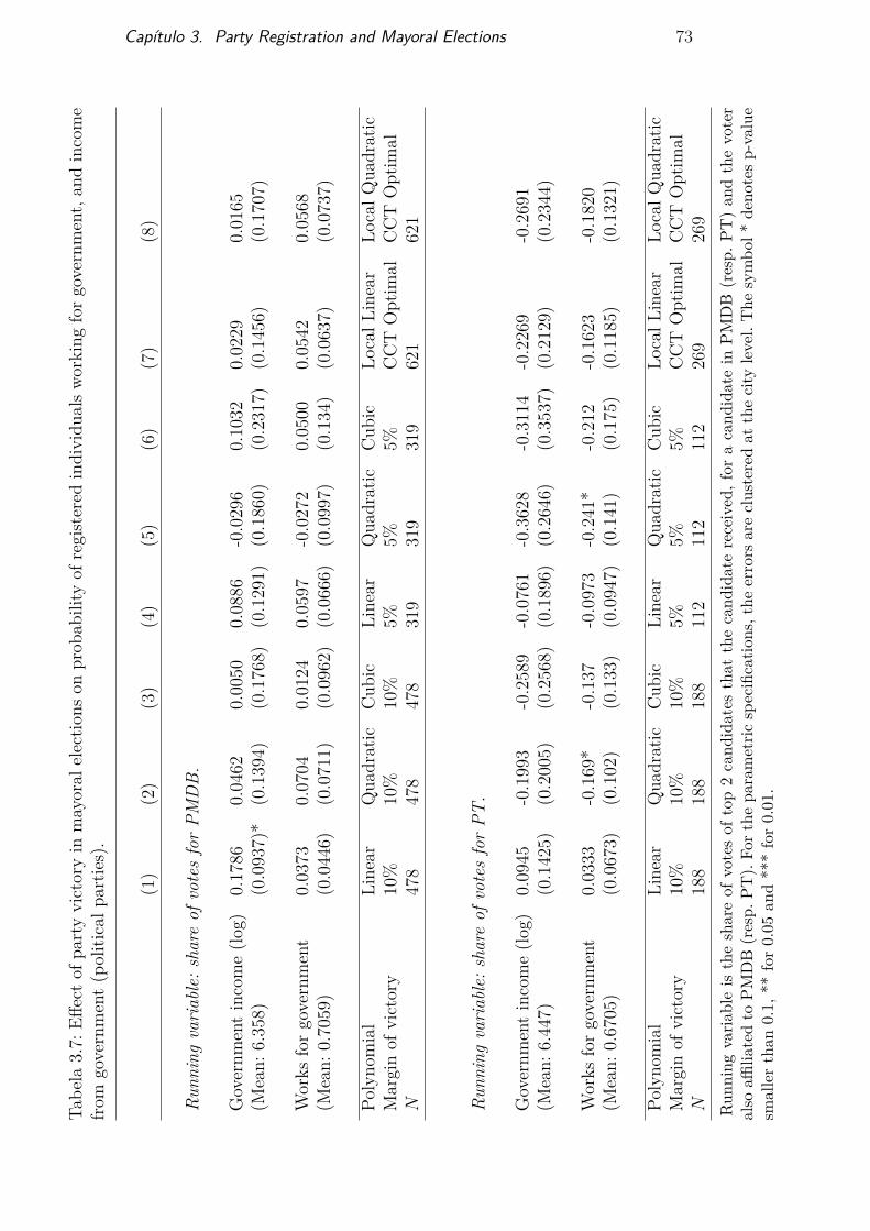
Capítulo 3. Party Registration and Mayoral Elections 73
Tabe
la3.7:
Effecto
fparty
victoryin
mayoral
electio
nson
prob
ability
ofregistered
individu
alsw
orking
forg
overnm
ent,an
dincome
from
government(politicalp
artie
s).
(1)
(2)
(3)
(4)
(5)
(6)
(7)
(8)
R unn
ingvariable:s
hare
ofvotesforPM
DB.
Governm
entincome(lo
g)0.17
860.04
620.00
500.08
86-0.029
60.10
320.02
290.01
65(M
ean:
6.35
8)(0.093
7)*
(0.139
4)(0.176
8)(0.129
1)(0.186
0)(0.231
7)(0.145
6)(0.1707)
Works
forgovernment
0.03
730.07
040.01
240.05
97-0.027
20.05
000.05
420.05
68(M
ean:
0.70
59)
(0.044
6)(0.071
1)(0.096
2)(0.066
6)(0.099
7)(0.134
)(0.063
7)(0.073
7)
P olyno
mial
Line
arQua
dratic
Cub
icLine
arQua
dratic
Cub
icLo
calL
inear
LocalQ
uadratic
Marginof
victory
10%
10%
10%
5%5%
5%CCT
Optim
alCCT
Optim
alN
478
478
478
319
319
319
621
621
R unn
ingvariable:s
hare
ofvotesforPT
.
Governm
entincome(lo
g)0.09
45-0.199
3-0.258
9-0.076
1-0.362
8-0.311
4-0.226
9-0.269
1(M
ean:
6.44
7)(0.142
5)(0.200
5)(0.2568)
(0.189
6)(0.264
6)(0.353
7)(0.212
9)(0.234
4)
Works
forgovernment
0.03
33-0.169
*-0.137
-0.097
3-0.241
*-0.212
-0.162
3-0.182
0(M
ean:
0.67
05)
(0.067
3)(0.102
)(0.133)
(0.094
7)(0.141
)(0.175
)(0.118
5)(0.132
1)
Polyno
mial
Line
arQua
dratic
Cub
icLine
arQua
dratic
Cub
icLo
calL
inear
LocalQ
uadratic
Marginof
victory
10%
10%
10%
5%5%
5%CCT
Optim
alCCT
Optim
alN
188
188
188
112
112
112
269
269
Run
ning
varia
bleis
theshareof
votesof
top2cand
idates
that
thecand
idatereceived
,for
acand
idatein
PMDB
(resp.
PT)an
dthevoter
also
affilia
tedto
PMDB
(resp.
PT).Fo
rthepa
rametric
specificatio
ns,the
errors
areclusteredat
thecity
level.The
symbo
l*de
notesp-value
smallerthan
0.1,
**for0.05
and***for0.01.
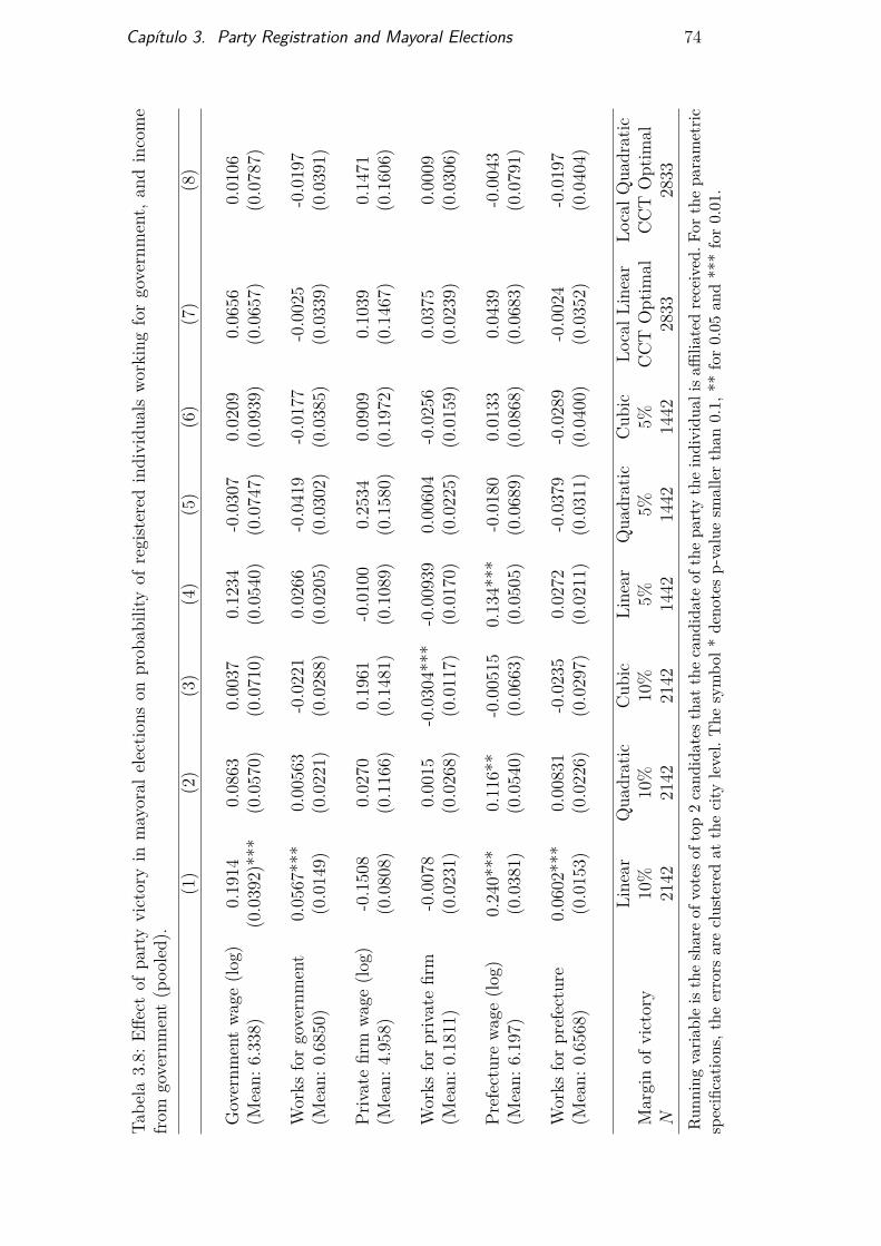
Capítulo 3. Party Registration and Mayoral Elections 74
Tabe
la3.8:
Effectof
partyvictoryin
mayoral
electio
nson
prob
ability
ofregistered
individu
alswo
rkingforgovernment,
andincome
from
government(poo
led).
(1)
(2)
(3)
(4)
(5)
(6)
(7)
(8)
Go vernm
entwa
ge(lo
g)0.1914
0.0863
0.0037
0.1234
-0.0307
0.0209
0.0656
0.0106
(Mean:
6.338)
(0.0392)***
(0.0570)
(0.0710)
(0.0540)
(0.0747)
(0.0939)
(0.0657)
(0.0787)
Works
forgovernment
0.0567***
0.00563
-0.0221
0.0266
-0.0419
-0.0177
-0.0025
-0.0197
(Mean:
0.6850)
(0.0149)
(0.0221)
(0.0288)
(0.0205)
(0.0302)
(0.0385)
(0.0339)
(0.0391)
Privatefirm
wage
(log)
-0.1508
0.0270
0.1961
-0.0100
0.2534
0.0909
0.1039
0.1471
(Mean:
4.958)
(0.0808)
(0.1166)
(0.1481)
(0.1089)
(0.1580)
(0.1972)
(0.1467)
(0.1606)
Works
forprivatefirm
-0.0078
0.0015
-0.0304***
-0.00939
0.00604
-0.0256
0.0375
0.0009
(Mean:
0.1811)
(0.0231)
(0.0268)
(0.0117)
(0.0170)
(0.0225)
(0.0159)
(0.0239)
(0.0306)
Prefecture
wage
(log)
0.240***
0.116**
-0.00515
0.134***
-0.0180
0.0133
0.0439
-0.0043
(Mean:
6.197)
(0.0381)
(0.0540)
(0.0663)
(0.0505)
(0.0689)
(0.0868)
(0.0683)
(0.0791)
Works
forprefecture
0.0602***
0.00831
-0.0235
0.0272
-0.0379
-0.0289
-0.0024
-0.0197
(Mean:
0.6568)
(0.0153)
(0.0226)
(0.0297)
(0.0211)
(0.0311)
(0.0400)
(0.0352)
(0.0404)
Linear
Qua
dratic
Cub
icLinear
Qua
dratic
Cub
icLo
calL
inear
LocalQ
uadratic
Marginof
victory
10%
10%
10%
5%5%
5%CCT
Optim
alCCT
Optim
alN
2142
2142
2142
1442
1442
1442
2833
2833
Run
ning
varia
bleistheshareof
voteso
ftop
2cand
idates
that
thecand
idateof
thepa
rtytheindividu
alisaffi
liatedreceived
.For
thepa
rametric
specificatio
ns,the
errors
areclusteredat
thecity
level.The
symbo
l*de
notesp-valuesm
allerthan
0.1,
**for0.05
and***for0.01.

Capítulo 3. Party Registration and Mayoral Elections 75
Before presenting the election results, we plot the local polynomialregression of number of registrations to a party after the election in a givencity on the proportion of votes for that party in the mayoral elections. Forthis plot, we take the logarithm of the number of registrations, for graphicalclarity. (In the regressions below, we use the absolute value of registrations,and the results are the same.) As is apparent in Figure 3.7, there seems to beno discontinuity in the number of registrations around the cutoff.
−0.4 −0.2 0.0 0.2 0.4
12
34
56
Proportion of votes for party in the presidential coalition.
Num
ber
of r
egis
trat
ions
afte
r el
ectio
n (lo
g).
Figura 3.7: Effect of mayoral victory on future party affiliations, for individualsregistered to parties in the presidential coalition.
We formalize the procedure of Figure 3.7 in Table 3.9. This table presentsthe results of parametrical and non-parametrical (local) polynomial RD designson the number of post-election registrations, the number of registrations inthe first year after the elections, and the number of registrations duringthe victorious mayor’s term. In none of these specification are the resultsstatistically significant or consistent between different designs.
We interpret these results as indicating that individuals do not perceiveaffiliation to the mayor’s party as providing any economic benefits, which isconsistent with us not finding any evidence of affiliates’ salary being any higherthan non-affiliates.
3.6Conclusion
In this paper, we have examined how registered members fo political par-ties are affected by their party’s victory in mayoral elections. We investigated
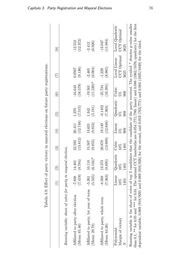
Capítulo 3. Party Registration and Mayoral Elections 76
Tabe
la3.9:
Effectof
partyvictoryin
mayoral
electio
nson
future
partyregistratio
ns.
(1)
(2)
(3)
(4)
(5)
(6)
(7)
(8)
Run
ning
vari
able
:sha
reof
vote
sfo
rpa
rty
inm
ayor
alel
ectio
n.
Affilia
tedto
partyafterelectio
n-7.938
14.401
22.592
20.411
1.37
0-24.643
0.0567
-12.552
(Mean:
65.46)
(7.419
)(8.784
)(13.81
2)(12.74
8)(7.515
)(16.579)
(9.136)
(12.372)
Affilia
tedto
party,
1styear
ofterm
-5.261
10.110
15.507
13.621
1.34
2-19.501
-2.465
-2.412
(Mean:
29.78)
(5.345
)(6.134
)*(9.855
)(8.853
)(5.181
)(11.530)*
(6.004)
(6.926)
Affilia
tedto
party,
who
leterm
-8.568
13.373
20.878
19.149
-0.140
2-25.734
-1.229
-13.047
(Mean:
64.26)
(7.363
)(8.695
)(13.68
9)(12.64
8)(7.363
)(16.391)
(8.985)
(11.884)
Polyno
mial
Line
arQua
dratic
Cub
icLine
arQua
dratic
Cub
icLo
calL
inear
LocalQ
uadratic
Marginof
victory
10%
10%
10%
5%5%
5%CCT
Optim
alCCT
Optim
alN
1401
1401
1401
909
909
909
3625
3625
Run
ning
varia
bleis
theshareof
votesof
top2cand
idates
that
thecand
idateof
thepa
rtyreceived
.The
symbo
l*de
notesp-valuesm
aller
than
0.1,
**for0.05
and***for0.01.T
heop
timal
CCT
band
with
sare0.05
4(771
/780
;linear)
and0.086(1062/1076;q
uadratic)forthefirst
depe
ndentvaria
ble,
0.069(918/929)an
d0.06
9(916
/926
)forthesecond
,and
0.05
3(763
/771)an
d0.083(1035/1049)forthethird
.
Capítulo 3. Party Registration and Mayoral Elections 77
the causal effect of the party an individual is affiliated to winning an electionon the probability of working for the government, on the wages accrued fromthe government, and on the number of future affiliations for that party in thatcity. In none of these cases we were able to find a discernible non-zero effect.
This might indicate that political parties do not have as much leeway forpatronage as previously thought, perhaps because of institutional constraints,as the need for public exams into bureaucracy and audits by governmentalagencies. Since most political affiliates are already public employees, if theyare hired by already specified contracts, the party might not have the powerto affect their wages, as they are defined by law. (This might be especiallythe case when there is a well defined career path, as with teachers or policeofficers.)
Another possibility is that bureaucracy appointments are slow, andtherefore supporters only acquire governmental jobs more than a year afterthe election, which we would not be able to capture with our current dataset.It is important to note, therefore, that this empirical exercise covers only the2008 mayoral elections for the Northeast of Brazil, and that we had access onlyto individual socioeconomic data for the years of 2008 and 2009. We hope, infuture research, to increase our database to cover all years for which the RAISis available, and to extend this analysis to all mayoral elections after the re-democratization. With that enlarged database, we would be able to ascertainmore confidently whether our results indicate absence of a treatment effect (asopposed to our inability to capture it), as well as being able to investigateheterogeneous effects according to city, party, and individual characteristics.
Referências Bibliográficas
[01] BISIN, A.; VERDIER, T.. Beyond the melting pot: Cultural trans-mission, marriage, and the evolution of ethnic and religioustraits. The Quarterly Journal of Economics, 115(3):955–988, 2000.
[02] BISIN, A.; VERDIER, T.. The economics of cultural transmission andthe dynamics of preferences. Journal of Economic Theory, 97(2):298–319, 2001.
[03] WEBER, M.. The Protestant ethic and the spirit of capitalism.Roxbury Los Angeles, 1998.
[04] BENABOU, R.; TIROLE, J.. Belief in a just world and redistributivepolitics. The Quarterly Journal of Economics, 121(2):699–746, 2006.
[05] ALESINA, A.; ANGELETOS, G.-M.. Fairness and redistribution. Ame-rican Economic Review, p. 960–980, 2005.
[06] BARRON, J. M.; GJERDE, K. P.. Peer pressure in an agency relati-onship. Journal of Labor economics, 15(2):234–54, 2008.
[07] ICHINO, A.; MAGGI, G.. Work environment and individual back-ground: explaining regional shirking differentials in a large ita-lian firm. The Quarterly Journal of Economics, 115(3):1057–1090, 2000.
[08] ROTEMBERG, J. J.. Human relations in the workplace. Journal ofPolitical Economy, p. 684–717, 1994.
[09] KANDEL, E.; LAZEAR, E. P.. Peer pressure and partnerships. Journalof political Economy, p. 801–817, 1992.
[10] LINDBECK, A.; NYBERG, S. ; WEIBULL, J. W.. Social norms andeconomic incentives in the welfare state. The Quarterly Journal ofEconomics, 114(1):1–35, 1999.
[11] FISCHER, P.; HUDDART, S.. Optimal contracting with endogenoussocial norms. The American Economic Review, 98(4):pp. 1459–1475, 2008.
Referências Bibliográficas 79
[12] HUCK, S.; KÜBLER, D. ; WEIBULL, J.. Social norms and economicincentives in firms. Journal of Economic Behavior & Organization,83(2):173–185, 2012.
[13] BISIN, A.; VERDIER, T.. Chapter 9 - the economics of culturaltransmission and socialization. volumen 1 de Handbook of SocialEconomics, p. 339 – 416. North-Holland, 2011.
[14] WEIBULL, J. W.. Evolutionary game theory. MIT press, 1997.
[15] CLARK, G.. A farewell to alms: a brief economic history of theworld. Princeton University Press, 2008.
[16] CLARK, G.. Why isn’t the whole world developed? lessons fromthe cotton mills. The Journal of economic history, 47(01):141–173, 1987.
[17] HAUK, E.; SAEZ-MARTI, M.. On the cultural transmission ofcorruption. Journal of Economic Theory, 107(2):311–335, 2002.
[18] LINDBECK, A.; NYBERG, S.. Raising children to work hard: al-truism, work norms, and social insurance. The Quarterly Journal ofEconomics, 121(4):1473–1503, 2006.
[19] BECKER, S. O.; WOESSMANN, L.. Was weber wrong? a humancapital theory of protestant economic history. The Quarterly Journalof Economics, 124(2):531–596, 2009.
[20] CANTONI, D.. The economic effects of the protestant reformation:Testing the weber hypothesis in the german lands. 2013.
[21] DOEPKE, M.; ZILIBOTTI, F.. Occupational choice and the spirit ofcapitalism. The Quarterly Journal of Economics, 123(2):747–793, 2008.
[22] KREMER, M.. The o-ring theory of economic development. TheQuarterly Journal of Economics, 108(3):551–575, 1993.
[23] STIGLER, G. J.; BECKER, G. S.. De gustibus non est disputandum.The American Economic Review, p. 76–90, 1977.
[24] TOPKIS, D. M.. Supermodularity and complementarity. PrincetonUniversity Press, 1998.
[25] BRYNJOLFSSON, E.; MILGROM, P.. Complementarity in organiza-tions. The Handbook of Organizational Economics, 11, 2012.
Referências Bibliográficas 80
[26] BRESNAHAN, T. F.; BRYNJOLFSSON, E. ; HITT, L. M.. Informationtechnology, workplace organization, and the demand for skilledlabor: Firm-level evidence. The Quarterly Journal of Economics,117(1):339–376, 2002.
[27] GROSHEN, E. L.. Sources of intra-industry wage dispersion: Howmuch do employers matter? The Quarterly Journal of Economics,106(3):869–884, 1991.
[28] CAVALLI-SFORZA, L. L.. Cultural transmission and evolution: Aquantitative approach. Número 16. Princeton University Press, 1981.
[29] BOYD, R.; RICHERSON, P.. Culture and the evolutionary process,1985.
[30] FRANKLIN, B.. Advice to a young tradesman, written by an oldone. The Writings of Benjamin Franklin: Philadelphia, 1726-1757, 2007.
[31] BAXTER, R.. A Christian directory, volumen I. Soli Deo GloriaPublications, 1996.
[32] HILLER, V.. Work organization, preferences dynamics and theindustrialization process. European Economic Review, 55(7):1007–1025,2011.
[33] MILGROM, P.; ROBERTS, J.. Rationalizability, learning, and equi-librium in games with strategic complementarities. Econometrica,58(6):1255–1277, 1990.
[34] MELTZER, A. H.; RICHARD, S. F.. A rational theory of the size ofgovernment. The Journal of Political Economy, p. 914–927, 1981.
[35] BENABOU, R.; OK, E. A.. Social mobility and the demand forredistribution: The poum hypothesis. The Quarterly Journal ofEconomics, 116(2):447–487, 2001.
[36] FONG, C.. Social preferences, self-interest, and the demand forredistribution. Journal of Public Economics, 82(2):225–246, 2001.
[37] LUTTMER, E. F.. Neighbors as negatives: Relative earnings andwell-being*. The Quarterly journal of economics, 120(3):963–1002, 2005.
[38] PIKETTY, T.. Social mobility and redistributive politics. TheQuarterly journal of economics, p. 551–584, 1995.
Referências Bibliográficas 81
[39] ALESINA, A.; LA FERRARA, E.. Preferences for redistribution inthe land of opportunities. Journal of Public Economics, 89(5):897–931,2005.
[40] ALESINA, A.; DI TELLA, R. ; MACCULLOCH, R.. Inequality andhappiness: are europeans and americans different? Journal of PublicEconomics, 88(9):2009–2042, 2004.
[41] CORNEO, G.; GRÜNER, H. P.. Social limits to redistribution. Ameri-can Economic Review, p. 1491–1507, 2000.
[42] CORNEO, G.; GRÜNER, H. P.. Individual preferences for politicalredistribution. Journal of public Economics, 83(1):83–107, 2002.
[43] ALESINA, A.; GLAESER, E.. Fighting poverty in the us and europe:A world of difference. 2004.
[44] MICHAEL S. LEWIS-BECK, T. W. R.. Localism in presidential electi-ons: The home state advantage. American Journal of Political Science,27(3):548–556, 1983.
[45] MILLO, G.; PIRAS, G.. splm: Spatial panel data models in r. Journalof Statistical Software, 47(1):1–38, 2012.
[46] KAPOOR, M.; KELEJIAN, H. H. ; PRUCHA, I. R.. Panel data modelswith spatially correlated error components. Journal of Econometrics,140(1):97 – 130, 2007. Analysis of spatially dependent data.
[47] GLAESER, E. L.; SACERDOTE, B. I. ; SCHEINKMAN, J. A.. The socialmultiplier. Journal of the European Economic Association, 1(2-3):345–353,2003.
[48] LEE, D. S.. Randomized experiments from non-random selectionin u.s. house elections. Journal of Econometrics, 142(2):675 – 697, 2008.The regression discontinuity design: Theory and applications.
[49] BESLEY, T.; PANDE, R. ; RAO, V.. Just rewards? local politics andpublic resource allocation in south india. The World Bank EconomicReview, 26(2):191–216, 2012.
[50] BET CAEYERS, S. D.. Political connections and social networksin targeted transfer programs: Evidence from rural ethiopia.Economic Development and Cultural Change, 60(4):639–675, 2012.
Referências Bibliográficas 82
[51] MARKUSSEN, T.; TARP, F.. Political connections and land-relatedinvestment in rural vietnam. Journal of Development Economics,110:291 – 302, 2014. Land and Property Rights.
[52] LEE, D. S.; LEMIEUX, T.. Regression discontinuity designs ineconomics. Journal of Economic Literature, 48(2):281–355, 2010.
[53] BUCHANAN, J. M.; TULLOCK, G.. The calculus of consent, volumen 3.University of Michigan Press Ann Arbor, 1962.
[54] LIZZERI, A.; PERSICO, N.. The provision of public goods underalternative electoral incentives. American Economic Review, p. 225–239, 2001.
[55] FOLKE, O.; HIRANO, S. ; SNYDER, J. M.. Patronage and elections inus states. American Political Science Review, 105(03):567–585, 2011.
[56] ENIKOLOPOV, R.. Politicians, bureaucrats and targeted redistri-bution. Journal of Public Economics, 120:74–83, 2014.
[57] ALESINA, A.; BAQIR, R. ; EASTERLY, W.. Redistributive publicemployment. Journal of Urban Economics, 48(2):219–241, 2000.
[58] COATE, S.; MORRIS, S.. On the form of transfers to specialinterests. Journal of political Economy, p. 1210–1235, 1995.
[59] ROBINSON, J. A.; VERDIER, T.. The political economy of cliente-lism. The Scandinavian Journal of Economics, 115(2):260–291, 2013.
[60] HILLER, V.; VERDIER, T.. Corporate culture and identity invest-ment in an industry equilibrium. Journal of Economic Behavior &Organization, 103:93–112, 2014.
[61] SÁEZ-MARTI, M.; ZENOU, Y.. Cultural transmission and discrimi-nation. Journal of Urban Economics, 72(2):137–146, 2012.
[62] GALOR, O.; MOAV, O.. Natural selection and the origin of economicgrowth. Quarterly Journal of Economics, p. 1133–1191, 2002.
[63] GALOR, O.; MICHALOPOULOS, S.. Evolution and the growth pro-cess: Natural selection of entrepreneurial traits. Journal of Econo-mic Theory, 147(2):759–780, 2012.
[64] DUR, R.; SOL, J.. Social interaction, co-worker altruism, andincentives. Games and Economic Behavior, 69(2):293–301, 2010.
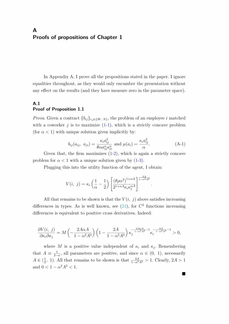
AProofs of propositions of Chapter 1
In Appendix A, I prove all the propositions stated in the paper. I ignoreequalities throughout, as they would only encumber the presentation withoutany effect on the results (and they have measure zero in the parameter space).
A.1Proof of Proposition 1.1
Prova. Given a contract {bij}i,j∈{W, N}, the problem of an employee i matchedwith a coworker j is to maximize (1-1), which is a strictly concave problem(for α < 1) with unique solution given implicitly by:
bij(aij, aji) =κia
2ij
θαaαijaαji
and µ(ai) =κia
2ij
α. (A-1)
Given that, the firm maximizes (1-2), which is again a strictly concaveproblem for α < 1 with a unique solution given by (1-3).
Plugging this into the utility function of the agent, I obtain:
V (i, j) = κi
( 1α− 1
2
) (θρα2)1+αA
21+αAκiκαAj
2A1−α2A2
.
All that remains to be shown is that the V (i, j) above satisfies increasingdifferences in types. As is well known, see (24), for C2 functions increasingdifferences is equivalent to positive cross derivatives. Indeed:
∂V (i, j)∂κi∂κj
= M(− 2AαA
1− α2A2
)(1− 2A
1− α2A2
)κ− 2AαA
1−α2A2−1j κ
− 2A1−α2A2−1
i > 0,
where M is a positive value independent of κi and κj. Rememberingthat A ≡ 1
2−α , all parameters are positive, and since α ∈ (0, 1), necessarilyA ∈ (1
2 , 1). All that remains to be shown is that 2A1−α2A2 > 1. Clearly, 2A > 1
and 0 < 1− α2A2 < 1.�
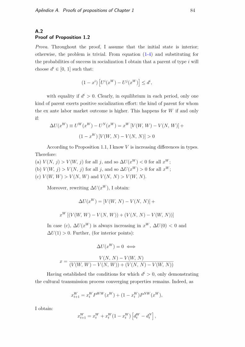
Apêndice A. Proofs of propositions of Chapter 1 84
A.2Proof of Proposition 1.2
Prova. Throughout the proof, I assume that the initial state is interior;otherwise, the problem is trivial. From equation (1-4) and substituting forthe probabilities of success in socialization I obtain that a parent of type i willchoose di ∈ [0, 1] such that:
(1− xi)[U i(xW )− U j(xW )
]≤ di,
with equality if di > 0. Clearly, in equilibrium in each period, only onekind of parent exerts positive socialization effort: the kind of parent for whomthe ex ante labor market outcome is higher. This happens for W if and onlyif:
∆U(xW ) ≡ UW (xW )− UN(xW ) = xW [V (W, W )− V (N, W )] +
(1− xW ) [V (W, N)− V (N, N)] > 0
According to Proposition 1.1, I know V is increasing differences in types.Therefore:(a) V (N, j) > V (W, j) for all j, and so ∆U(xW ) < 0 for all xW ;(b) V (W, j) > V (N, j) for all j, and so ∆U(xW ) > 0 for all xW ;(c) V (W, W ) > V (N, W ) and V (N, N) > V (W, N).
Moreover, rewriting ∆U(xW ), I obtain:
∆U(xW ) = [V (W, N)− V (N, N)] +
xW [(V (W, W )− V (N, W )) + (V (N, N)− V (W, N))]
In case (c), ∆U(xW ) is always increasing in xW , ∆U(0) < 0 and∆U(1) > 0. Further, (for interior points):
∆U(xW ) = 0 ⇐⇒
x = V (N, N)− V (W, N)(V (W, W )− V (N, W )) + (V (N, N)− V (W, N))
Having established the conditions for which di > 0, only demonstratingthe cultural transmission process converging properties remains. Indeed, as
xWt+1 = xWt PWW (xW ) + (1− xWt )PNW (xW ),
I obtain:xWt+1 = xWt + xWt (1− xWt )
[dWt − dNt
],
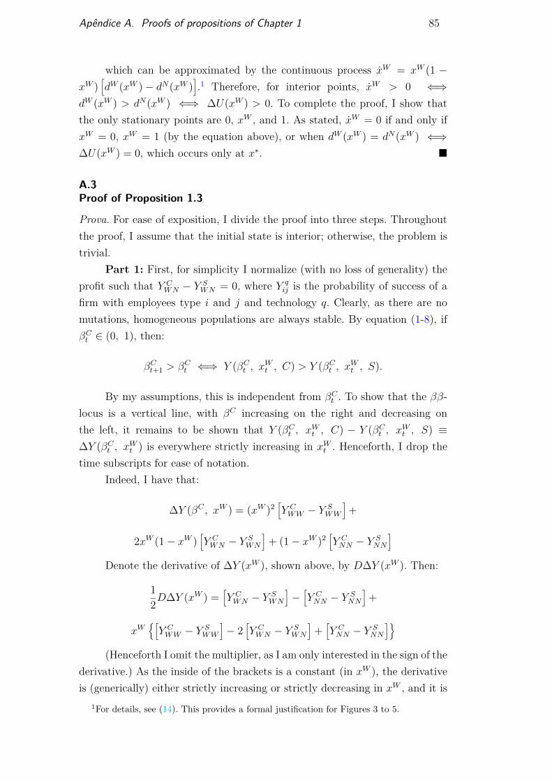
Apêndice A. Proofs of propositions of Chapter 1 85
which can be approximated by the continuous process xW = xW (1 −xW )
[dW (xW )− dN(xW )
].1 Therefore, for interior points, xW > 0 ⇐⇒
dW (xW ) > dN(xW ) ⇐⇒ ∆U(xW ) > 0. To complete the proof, I show thatthe only stationary points are 0, xW , and 1. As stated, xW = 0 if and only ifxW = 0, xW = 1 (by the equation above), or when dW (xW ) = dN(xW ) ⇐⇒∆U(xW ) = 0, which occurs only at x∗. �
A.3Proof of Proposition 1.3
Prova. For ease of exposition, I divide the proof into three steps. Throughoutthe proof, I assume that the initial state is interior; otherwise, the problem istrivial.
Part 1: First, for simplicity I normalize (with no loss of generality) theprofit such that Y C
WN − Y SWN = 0, where Y q
ij is the probability of success of afirm with employees type i and j and technology q. Clearly, as there are nomutations, homogeneous populations are always stable. By equation (1-8), ifβCt ∈ (0, 1), then:
βCt+1 > βCt ⇐⇒ Y (βCt , xWt , C) > Y (βCt , xWt , S).
By my assumptions, this is independent from βCt . To show that the ββ-locus is a vertical line, with βC increasing on the right and decreasing onthe left, it remains to be shown that Y (βCt , xWt , C) − Y (βCt , xWt , S) ≡∆Y (βCt , xWt ) is everywhere strictly increasing in xWt . Henceforth, I drop thetime subscripts for ease of notation.
Indeed, I have that:
∆Y (βC , xW ) = (xW )2[Y CWW − Y S
WW
]+
2xW (1− xW )[Y CWN − Y S
WN
]+ (1− xW )2
[Y CNN − Y S
NN
]Denote the derivative of ∆Y (xW ), shown above, by D∆Y (xW ). Then:
12D∆Y (xW ) =
[Y CWN − Y S
WN
]−[Y CNN − Y S
NN
]+
xW{[Y CWW − Y S
WW
]− 2
[Y CWN − Y S
WN
]+[Y CNN − Y S
NN
]}(Henceforth I omit the multiplier, as I am only interested in the sign of the
derivative.) As the inside of the brackets is a constant (in xW ), the derivativeis (generically) either strictly increasing or strictly decreasing in xW , and it is
1For details, see (14). This provides a formal justification for Figures 3 to 5.

Apêndice A. Proofs of propositions of Chapter 1 86
sufficient to evaluate the equation above at the corners (i.e., with xW equaling0 or 1). A necessary and sufficient condition for the above derivative to bepositive everywhere is that
[Y CWW − Y S
WW
]>[Y CWN − Y S
WN
]>[Y CNN − Y S
NN
],
or under my normalization, that:
[Y CWW − Y S
WW
]> 0 >
[Y CNN − Y S
NN
].
I start by noting that (under my normalization) ∆Y (1) = Y CWW − Y S
WW
and ∆Y (0) = Y CNN − Y S
NN . Note also that D∆Y (1) = Y CWW − Y S
WW andD∆Y (0) = −
[Y CNN − Y S
NN
], and that D∆Y (xW ) is a linear combinations of
both.There are four possible cases:
(i) Y CWW − Y S
WW > 0 and Y CNN − Y S
NN > 0;(ii) Y C
WW − Y SWW > 0 and Y C
NN − Y SNN < 0;
(iii) Y CWW − Y S
WW < 0 and Y CNN − Y S
NN > 0; and(iv) Y C
WW − Y SWW < 0 and Y C
NN − Y SNN < 0.
Thus, I now show that: a) case (iii) is impossible and that b) in cases (i)and (iv) ∆Y (xW ) has no root.
a) The revenue of the firm with complementary technology is given by:
Y (κi, κj) = ρθ
(θρα2)1+αA
21+αAκiκαAj
αA1−α2A2
(θρα2)1+αA
21+αAκjκαAi
αA1−α2A2
Now, I show that Y (κi, κj) is increasing differences in κi and κj, andY Sij = Y S
i + Y Sj (a trivial consequence of separability). Indeed:
∂Y Cij
∂i∂j=[−(1 + αA) αA
1− α2A2
]2Cκ−(1+αA) αA
1−α2A2−1i κ
−(1+αA) αA1−α2A2−1
j > 0,
where C is a positive constant (in (κi, κj)).b) For (i), D∆Y (1) ≥ D∆Y (xW ) for all xW (as they are a linear
combination of D∆Y (1) > 0 and D∆Y (0) < 0). By the Fundamental Theoremof Calculus, if there was a y between 0 and 1 such that ∆Y (y) = 0, then:
∆Y (1) = ∆Y (1)−∆Y (y) =∫ 1
yD∆Y (x) dx ≤
∫ 1
yD∆Y (1) dx = (1− y)∆Y (1) < ∆Y (1),
which is a contradiction. (Here, I useD∆Y (1) = ∆Y (1).) Analogously, for (iv),D∆Y (xW ) ≤ D∆Y (0), and thus, if there is y ∈ (0, 1) such that ∆Y (y) = 0,
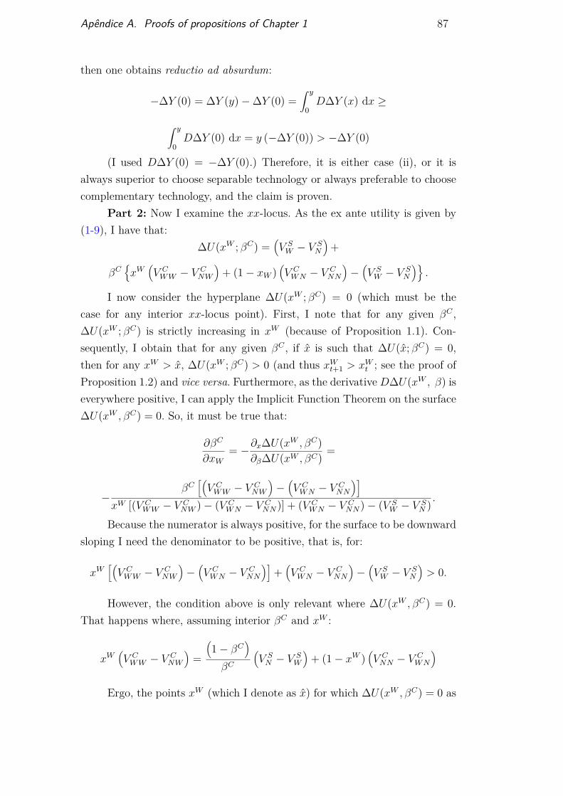
Apêndice A. Proofs of propositions of Chapter 1 87
then one obtains reductio ad absurdum:
−∆Y (0) = ∆Y (y)−∆Y (0) =∫ y
0D∆Y (x) dx ≥
∫ y
0D∆Y (0) dx = y (−∆Y (0)) > −∆Y (0)
(I used D∆Y (0) = −∆Y (0).) Therefore, it is either case (ii), or it isalways superior to choose separable technology or always preferable to choosecomplementary technology, and the claim is proven.
Part 2: Now I examine the xx-locus. As the ex ante utility is given by(1-9), I have that:
∆U(xW ; βC) =(V SW − V S
N
)+
βC{xW
(V CWW − V C
NW
)+ (1− xW )
(V CWN − V C
NN
)−(V SW − V S
N
)}.
I now consider the hyperplane ∆U(xW ; βC) = 0 (which must be thecase for any interior xx-locus point). First, I note that for any given βC ,∆U(xW ; βC) is strictly increasing in xW (because of Proposition 1.1). Con-sequently, I obtain that for any given βC , if x is such that ∆U(x; βC) = 0,then for any xW > x, ∆U(xW ; βC) > 0 (and thus xWt+1 > xWt ; see the proof ofProposition 1.2) and vice versa. Furthermore, as the derivativeD∆U(xW , β) iseverywhere positive, I can apply the Implicit Function Theorem on the surface∆U(xW , βC) = 0. So, it must be true that:
∂βC
∂xW= −∂x∆U(xW , βC)
∂β∆U(xW , βC) =
−βC
[(V CWW − V C
NW
)−(V CWN − V C
NN
)]xW [(V C
WW − V CNW )− (V C
WN − V CNN)] + (V C
WN − V CNN)− (V S
W − V SN ) .
Because the numerator is always positive, for the surface to be downwardsloping I need the denominator to be positive, that is, for:
xW[(V CWW − V C
NW
)−(V CWN − V C
NN
)]+(V CWN − V C
NN
)−(V SW − V S
N
)> 0.
However, the condition above is only relevant where ∆U(xW , βC) = 0.That happens where, assuming interior βC and xW :
xW(V CWW − V C
NW
)=
(1− βC
)βC
(V SN − V S
W
)+ (1− xW )
(V CNN − V C
WN
)
Ergo, the points xW (which I denote as x) for which ∆U(xW , βC) = 0 as

Apêndice A. Proofs of propositions of Chapter 1 88
a function of βC are:
x =
(V CNN − V C
WN
)+ (1−βC)
βC
(V SN − V S
W
)(V C
WW − V CNW )− (V C
WN − V CNN) .
(Here, I inverted the V CNN − V C
WN term.) So, the condition is that for allx satisfying this, that:
∂∆U(xW ; βC)∂βC
= x[(V CWW − V C
NW
)−(V CWN − V C
NN
)]+
[(V CWN − V C
NN
)−(V SW − V S
N
)]> 0
⇐⇒
(1− βC
)βC
(V SN − V S
W
)+(V SN − V S
W
)> 0
(Again, some terms were inverted.) This always happens when V SN > V S
W ,and my proof is complete. �
A.4Proof of Proposition 1.4
Prova.I show that ∂[V (W, j)−V (N, j)]
∂ξ> 0, for ξ ≡ θρ (i.e. V is increasing
differences in the agent’s type and the parameters). The other two assertionsare trivial, since they impact directly the relative payoffs of the different types.Indeed:
V (W, j)− V (N, j) = ξ(1+αA) 2A
1−α2A2 [F (κW )− F (κN)] ,
where
F (κi) ≡ κi
( 1α− 1
2
) (α2)1+αA
21+αAκiκαAj
2A1−α2A2
is an everywhere decreasing function of κi (as 2A1−α2A2 > 0, as proved with
Proposition 1.1), so the derivative is everywhere positive, as κW < κN . �
BFurther specifications for Chapter 2
As explained in the main text, both main empirical strategies in thispaper, namely the use of spatial data models and tract-year dummies, areunfeasible using the entire dataset I have. Therefore, in the main paper I haverestricted attention to Ohio, which is a populous and densely populated swingstate of United States. In this Appendix I show evidence that Ohio indeedrepresents the entire United States, by showing results that are consistent withthe ones found in the main paper. More specifically, here I employ the samespecification as in the main text, but with data for the entire United States,using county-level time-varying dummies (as opposed to tract-level, which arefiner).
It is important to note that since precinct-level election data was notprovided by all states, I have only 31 states in our sample for 2008 (116,214precincts). Furthermore, since precincts change over time, I were only able toadequately match precinct-level data for 18 states for 2004 and 2008 elections(56,781), and for 10 states for 2004 through 2012 elections (30,713 precincts).
I use this data to build three balanced databases. I first call D1 thedatabase containing all precincts for 2008. I then build a balanced panel withthe precincts for which both 2004 and 2008 data are available, and call it D2.Finally, I do the same for the precincts for which data for all three electionsis available (D3). Moreover, as our interpretation of neighboring precincts asneighbors suggests that the effect should be present when precincts are smaller,I restrict the sample for urban areas, as defined by the census, in databasesD1 and D2. Since they have less overall observations, I do not do the same forD3, nor for the regressions in the main text (using Ohio).
As it is clear in Table B.1, the results for our entire dataset are quali-tatively similar to what we find for Ohio (and quantitatively stronger). Thissubstantiates our choice of Ohio as a representative state of the entire UnitedStates, which is consistent with their place as swing state and bellwether ofUnited States Presidential Elections. It also shows that our results have exter-nal validity, as they are robust to the choice of particular subset of our entiredata we use in our empirical analysis.
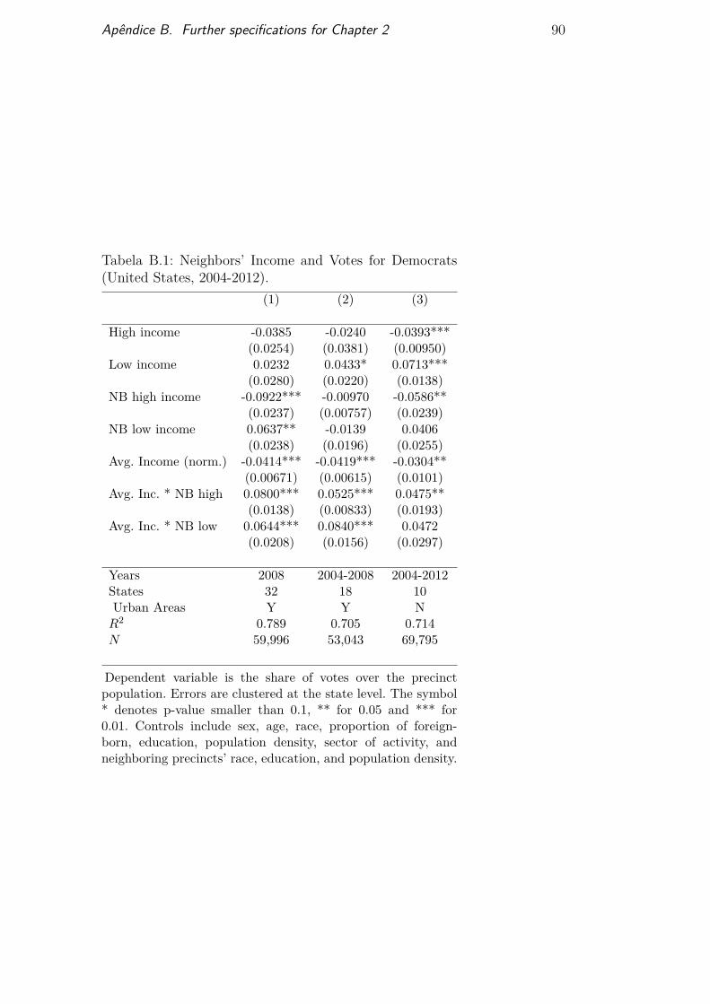
Apêndice B. Further specifications for Chapter 2 90
Tabela B.1: Neighbors’ Income and Votes for Democrats(United States, 2004-2012).
(1) (2) (3)
High income -0.0385 -0.0240 -0.0393***(0.0254) (0.0381) (0.00950)
Low income 0.0232 0.0433* 0.0713***(0.0280) (0.0220) (0.0138)
NB high income -0.0922*** -0.00970 -0.0586**(0.0237) (0.00757) (0.0239)
NB low income 0.0637** -0.0139 0.0406(0.0238) (0.0196) (0.0255)
Avg. Income (norm.) -0.0414*** -0.0419*** -0.0304**(0.00671) (0.00615) (0.0101)
Avg. Inc. * NB high 0.0800*** 0.0525*** 0.0475**(0.0138) (0.00833) (0.0193)
Avg. Inc. * NB low 0.0644*** 0.0840*** 0.0472(0.0208) (0.0156) (0.0297)
Years 2008 2004-2008 2004-2012States 32 18 10Urban Areas Y Y NR2 0.789 0.705 0.714N 59,996 53,043 69,795
Dependent variable is the share of votes over the precinctpopulation. Errors are clustered at the state level. The symbol* denotes p-value smaller than 0.1, ** for 0.05 and *** for0.01. Controls include sex, age, race, proportion of foreign-born, education, population density, sector of activity, andneighboring precincts’ race, education, and population density.