People, Wildlife and Livestock in the Mara Ecosystem: the Mara Count 2002

Report and analysis contributors:

Reid, R.S., Rainy, M., Ogutu, J., Kruska, R.L., Kimani, K., Nyabenge, M., McCartney, M., Kshatriya, M., Worden, J., Ng’ang’a, L., Owuor, J., Kinoti, J., Njuguna, E., Wilson, C.J., and Lamprey, R.

June 2003 (Version 1)

2

Copyright © Mara Count 2002. All rights reserved. Maps, graphics and text from this report may be reproduced for non-commercial use provided

that such reproduction shall acknowledge the Mara count 2002 with this citation: Reid, R.S., Rainy, M., Ogutu, J., Kruska, R.L., Kimani, K., Nyabenge, M., McCartney, M., Kshatriya, M., Worden, J., Ng’ang’a, L., Owuor, J., Kinoti, J.,

Njuguna, E., Wilson, C.J., and Lamprey, R. (2003). People, Wildlife and Livestock in the Mara Ecosystem: the Mara Count 2002. Report, Mara Count 2002, International Livestock Research Institute, Nairobi, Kenya.

3

Table of contents 1. Summary.............................................................................................................................................................................................................................. 12 2. Why count? (Introduction)................................................................................................................................................................................................. 14

2.1 Wildlife are being lost and pastoral peoples are poorer...................................................................................................................................................... 14 2.2 Recent changes in land use in the Serengeti-Mara Ecosystem........................................................................................................................................... 14 2.3 Why count people, livestock and wildlife?......................................................................................................................................................................... 15 2.4 Send us your comments ...................................................................................................................................................................................................... 15

3. What did we do and how did we do it? (Methods) ........................................................................................................................................................... 16 3.1 Counting area...................................................................................................................................................................................................................... 16 3.2 Counting methods in 1999 and 2002 .................................................................................................................................................................................. 16 3.3 Animal species we counted ................................................................................................................................................................................................ 19 3.4 Other information collected................................................................................................................................................................................................ 19 3.5 What does this method count well and what does it miss?................................................................................................................................................. 20 3.6 How we analysed the count data ........................................................................................................................................................................................ 21

4. What did we find and what might it mean? (Results and discussion) ............................................................................................................................ 23 4.1 General comments about the count information................................................................................................................................................................. 23 4.2 How many people, livestock and wildlife were counted altogether in 2002? .................................................................................................................... 23 4.3 People, bomas and huts: where and how many, now and in the past ................................................................................................................................. 23 4.4 Rainfall and the location of water, fences, farms, burns and tsetse flies ............................................................................................................................ 32 4.5 Location of tourist lodges, other infrastructure, vehicles and rubbish................................................................................................................................ 36 4.6 Height, amount (cover) and colour of grass, trees and shrubs............................................................................................................................................ 46 4.7 Livestock: how many and where? ...................................................................................................................................................................................... 58 4.8 Wildlife and multiple species associations (MSA’s): how many and where?.................................................................................................................... 67 4.9 How were types of wildlife and MSA’s distributed around the counting area?................................................................................................................. 67 4.10 How were individual species distributed around the counting area?................................................................................................................................ 74 4.11 Private compared with communal ranching ..................................................................................................................................................................... 78 4.12 Transmara (Triangle) compared with Narok part of the reserve ...................................................................................................................................... 78 4.14 Carcasses ........................................................................................................................................................................................................................ 114 4.16 How are wildlife distributed around bomas in the reserve and group ranches? ............................................................................................................. 124

5. Conclusions ........................................................................................................................................................................................................................ 129 5.1 How is pastoralism affecting wildlife in the Mara and how is wildlife affecting pastoralism in the Mara? .................................................................... 129

4

5.2 What does all this information suggest about management of the Mara? ........................................................................................................................ 129 5.3 Further information and discussion needed ...................................................................................................................................................................... 131

6. References .......................................................................................................................................................................................................................... 132 7. Appendix ............................................................................................................................................................................................................................ 137

5

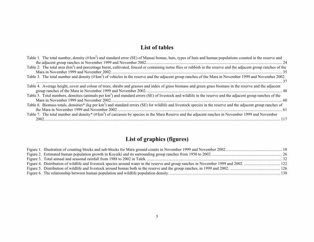
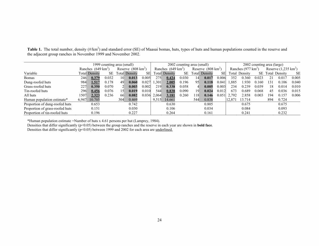
List of tables Table 1. The total number, density (#/km2) and standard error (SE) of Maasai bomas, huts, types of huts and human populations counted in the reserve and

the adjacent group ranches in November 1999 and November 2002.................................................................................................................................... 24 Table 2. The total area (km2) and percentage burnt, cultivated, fenced or containing tsetse flies or rubbish in the reserve and the adjacent group ranches of the

Mara in November 1999 and November 2002. ..................................................................................................................................................................... 35 Table 3. The total number and density (#/km2) of vehicles in the reserve and the adjacent group ranches of the Mara in November 1999 and November 2002.

............................................................................................................................................................................................................................................... 37 Table 4. Average height, cover and colour of trees, shrubs and grasses and index of grass biomass and green grass biomass in the reserve and the adjacent

group ranches of the Mara in November 1999 and November 2002. ................................................................................................................................... 48 Table 5. Total numbers, densities (animals per km2) and standard errors (SE) of livestock and wildlife in the reserve and the adjacent group ranches of the

Mara in November 1999 and November 2002. ..................................................................................................................................................................... 60 Table 6. Biomass totals, densities* (kg per km2) and standard errors (SE) for wildlife and livestock species in the reserve and the adjacent group ranches of

the Mara in November 1999 and November 2002. ............................................................................................................................................................... 61 Table 7. The total number and density* (#/km2) of carcasses by species in the Mara Reserve and the adjacent ranches in November 1999 and November

2002..................................................................................................................................................................................................................................... 117

List of graphics (figures) Figure 1. Illustration of counting blocks and sub-blocks for Mara ground counts in November 1999 and November 2002....................................................... 18 Figure 2. Estimated human population growth in Koyaiki and its surrounding group ranches from 1950 to 2002. .................................................................... 26 Figure 3. Total annual and seasonal rainfall from 1988 to 2002 in Talek. ................................................................................................................................... 32 Figure 4. Distribution of wildlife and livestock species around water in the reserve and group ranches in November 1999 and 2002. ................................... 122 Figure 5. Distribution of wildlife and livestock around bomas both in the reserve and the group ranches, in 1999 and 2002. ................................................. 126 Figure 6. The relationship between human population and wildlife population density. ........................................................................................................... 130

6

List of maps Map 1. Study area for the 1999 and 2002 counts showing Mara reserve and group ranches. ...................................................................................................... 17 Map 2. Distribution of pastoral bomas (settlements) in the count area, November, 2002............................................................................................................ 27 Map 3. Mean number of huts in each boma in the count area, November, 2002. ........................................................................................................................ 28 Map 4. Percentage of huts with dung roofs in each boma in the count area, November, 2002. ................................................................................................... 29 Map 5. Percentage of huts with grass roofs in each boma in the count area, November, 2002.................................................................................................... 30 Map 6. Percentage of huts with tin roof in each boma in the count area, November, 2002. ........................................................................................................ 31 Map 7. Sources of surface water in the count area between 9-16 November 2002, as recorded during aerial surveys. .............................................................. 33 Map 8. Sources of surface water as recorded by ground counting teams between 9-16 November, 2002................................................................................... 34 Map 9. Distribution of cropland in the count area, November, 2002. .......................................................................................................................................... 38 Map 10. Distribution of fenced areas (cropped plus not cropped) in the count area, November, 2002........................................................................................ 39 Map 11. Areas burned by bush fires at different times before the count. ..................................................................................................................................... 40 Map 12. Distribution of tsetse flies in the count area, November, 2002....................................................................................................................................... 41 Map 13. Distribution and types of tourist lodges in the count area, November, 2002.................................................................................................................. 42 Map 14. Distribution of other infrastructure in the count area, November, 2002......................................................................................................................... 43 Map 15. Presence and absence of rubbish (plastic bags, paper) in the count area, November, 2002. .......................................................................................... 44 Map 16. Distribution of motor vehicles during the count in November, 2002. ............................................................................................................................ 45 Map 17. Percentage cover of grass in the count area, November, 2002. ...................................................................................................................................... 49 Map 18. Height of grass (in centimeters) at block level (1km2) in the count area, November, 2002. ........................................................................................... 50 Map 19. Colour of the grass (percentage green) at the block level (1 km2) in the count area, November, 2002. ......................................................................... 51 Map 20. Percentage of ground covered by shrubs at block level (1 km2) in the count area, November, 2002. ............................................................................ 52 Map 21. Height of shrubs (in meteres) at block level (1 km2) in the count area, November, 2002............................................................................................... 53 Map 22. Colour of shrub leaves (percentage green) at block level (1 km2) in the count area, November, 2002........................................................................... 54 Map 23. Percentage of ground covered by trees at block level (1 km2) in the count area, November, 2002. ............................................................................... 55 Map 24. Height of trees (in meteres) at block level (1 km2) in the count area, November, 2002.................................................................................................. 56 Map 25. Colour of tree leaves (percentage green) at block level (1 km2) in the count area, November, 2002. ............................................................................ 57 Map 26. Number of cattle per sub-block (0.11 km2) in the count area, November, 2002. ............................................................................................................ 62 Map 27. Number of sheep and goats (shoats) per sub-block (0.11 km2) in the count area, November, 2002. .............................................................................. 63 Map 28. Number of donkeys per sub-block (0.11 km2) in the count area, November, 2002. ....................................................................................................... 64 Map 29. Number of domestic dogs per sub-block (0.11 km2) in the count area, November, 2002............................................................................................... 65 Map 30. Aggregated livestock biomass in kg/ km2 in the count area, November, 2002. .............................................................................................................. 66

7

Map 31. Aggregated wild herbivore biomass in kg/ km2 in the count area, November, 2002. ..................................................................................................... 70 Map 32. Aggregated wild carnivore biomass in kg/ km2 in the count area, November, 2002....................................................................................................... 71 Map 33. Number of wildlife species per sub-block (0.11 km2) in the count area, November, 2002. ............................................................................................ 72 Map 34. Distribution of multiple species associations in the count area, November, 2002. ......................................................................................................... 73 Map 35. Number of wildebeest per sub-block (0.11 km2) in the count area, November, 2002. ................................................................................................... 79 Map 36. Number of Burchell’s zebra per sub-block (0.11 km2) in the count area, November, 2002........................................................................................... 80 Map 37. Number of hippo per sub-block (0.11 km2) in the count area, November, 2002. ........................................................................................................... 81 Map 38. Number of Cape buffalo per sub-block (0.11 km2) in the count area, November, 2002. ............................................................................................... 82 Map 39. Number of Defassa waterbuck per sub-block (0.11 km2) in the count area, November, 2002....................................................................................... 83 Map 40. Number of Coke’s hartebeest per sub-block (0.11 km2) in the count area, November, 2002......................................................................................... 84 Map 41. Number of Maasai ostrich sub-block (0.11 km2) in the count area, November, 2002................................................................................................... 85 Map 42. Number of topi per sub-block (0.11 km2) in the count area, November, 2002. .............................................................................................................. 86 Map 43. Number of warthog per sub-block (0.11 km2) in the count area, November, 2002. ....................................................................................................... 87 Map 44. Number of Bohor reedbuck per sub-block (0.11 km2) in the count area, November, 2002. .......................................................................................... 88 Map 45. Number of Thomson's gazelle per sub-block (0.11 km2) in the count area, November, 2002. ...................................................................................... 89 Map 46. Number of tortoise per sub-block (0.11 km2) in the counting area, November, 2002. ................................................................................................... 90 Map 47. Number of African elephant per sub-block (0.11 km2) in the count area, November, 2002. ......................................................................................... 91 Map 48. Number of Cape eland per sub-block (0.11 km2) in the count area, November, 2002. .................................................................................................. 92 Map 49. Number of Grant’s gazelle per sub-block (0.11 km2) in the count area, November, 2002............................................................................................. 93 Map 50. Number of impala per sub-block (0.11 km2) in the count area, November, 2002. ......................................................................................................... 94 Map 51. Number of Eastern bushbuck per sub-block (0.11 km2) in the count area, November, 2002......................................................................................... 95 Map 52. Number of duiker (all species)per sub-block (0.11 km2) in the count area, November, 2002..................................................................................... 96 Map 53. Number of oribi per sub-block (0.11 km2) in the count area, November, 2002.............................................................................................................. 97 Map 54. Number of hare (all species) per sub-block (0.11 km2) in the count area, November, 2002. ......................................................................................... 98 Map 55. Number of Maasai giraffe per sub-block (0.11 km2) in the count area, November, 2002. ............................................................................................. 99 Map 56. Number of black rhino per sub-block (0.11 km2) in the count area, November, 2002. ................................................................................................ 100 Map 57. Number of Kirk’s dik-dik per sub-block (0.11 km2) in the count area, November, 2002. .......................................................................................... 101 Map 58. Number of lion per sub-block (0.11 km2) in the count area, November, 2002. ............................................................................................................ 102 Map 59. Number of crocodile per sub-block (0.11 km2) in the count area, November, 2002. ................................................................................................... 103 Map 60. Number of leopard per sub-block (0.11 km2) in the count area, November, 2002. ...................................................................................................... 104 Map 61. Number of cheetah per sub-block (0.11 km2) in the count area, November, 2002. ...................................................................................................... 105 Map 62. Number of spotted hyena per sub-block (0.11 km2) in the count area, November, 2002. ............................................................................................ 106

8

Map 63. Number of jackal species per sub-block (0.11 km2) in the count area,November, 2002. ............................................................................................. 107 Map 64. Number of honey badger per sub-block (0.11 km2) in the count area, November, 2002. ............................................................................................ 108 Map 65. Number of bat-eared fox per sub-block (0.11 km2) in the count area, November, 2002. ............................................................................................. 109 Map 66. Number of vulture (all species) per sub-block (0.11 km2) in the count area, November, 2002.................................................................................... 110 Map 67. Number of mongoose (all species) per sub-block (0.11 km2) in the count area, November, 2002............................................................................... 111 Map 68. Number of Anubis baboon per sub-block (0.11 km2) in the count area, November, 2002........................................................................................... 112 Map 69. Number of vervet monkey per sub-block (0.11 km2) in the count area, November, 2002. .......................................................................................... 113 Map 70. Number of fresh carcasses per sub-block (0.11 km2) in the count area, November, 2002. .......................................................................................... 116 Map 71. Distance to the nearest water source (in kilometres) in the count area, November, 2002. ............................................................................................ 121 Map 72. Distance to the nearest boma (in kilometres) in the count area, November, 2002. ....................................................................................................... 128

9

Appendix Table A 1. Scientific and English names and weights of the 43 species of wildlife and livestock counted in the Mara Reserve and group ranches in 1999 and

2002..................................................................................................................................................................................................................................... 138 Table A 2. Number of animals counted by each ground counting team during November 2002............................................................................................... 139 Table A 3. The total number and density (number per km2) of Maasai bomas and huts by sectors of the Mara Reserve and adjacent ranches, and the estimated

human population size and density in November 2002....................................................................................................................................................... 140 Table A 4. The total number and density* (animals per km2) of animals by species in each sector of the Mara Reserve and adjacent ranches in the entire and

larger counting area in November 2002. ............................................................................................................................................................................. 141 Table A 5. The total biomass and biomass density* (kg per km2, SE= standard error) by species and by functional categories of species in each sector of the

Mara Reserve and adjacent ranches in November 2002. .................................................................................................................................................... 142 Table A 6. The total number and density* (number per km2) of carcasses by species for each sector of the Mara Reserve and the adjacent ranches in

November 2002. .................................................................................................................................................................................................................. 143

10

Acknowledgments Well done! The Mara count 2002 was truly a team effort in every sense of the word. The count owes its existence and success to the 22 vehicle counting teams, 3 aircraft counting teams, 20 organisations and 84 individuals who counted in the rain and mud and contributed vehicles, lodging, airplanes, communications equipment, food, t-shirts, writing and filming expertise, GIS and statistical analysis help, counting practice help and venue, fuel, website help, engineering expertise, and moral support. We were all overwhelmed with the support and good will given so freely by so many. We list the people here who contributed and we give this report to you: this is your hard work and your accomplishment! We say a very big ‘thank you’ to all involved. It was an honour and pleasure to work with you. Mara Count 2002 supporters Overall count sponsors: Rainy family, Campfire Conservation, Narok County Council, Mara Wildlife Trusts, Koyiaki Group Ranch, Olkinyei Group Ranch, and the International Livestock Research Institute (ILRI).

Vehicle sponsors: Bike Treks Ltd, Mara Conservancy, Mrigesh Kshatriya, Wildlife Works, Abercrombie and Kent, Grant & Cameron Safaris, Campfire Conservation Ltd, African Conservation Centre, Sirata Sirua Ltd, Swara Plains Corp, Amara Conservation Ltd, Kobo Safaris, Friends of Conservation, Anne Kent Taylor Foundation/ A.K. Taylor International, International Livestock Research Institute, Vuorio/Mikkonen, World Wide Fund for Nature, Explore Mara Ltd., Jeff & Jessica Worden, Russ Kruska, Robin Reid, Cathy Wilson, Basecamp Masai Mara.

Local Maasai counters were from: Mara Conservancy, Koyiaki Group Ranch, Olkinyei Group Ranch, NCC Reserve, and Ol Chorro Oiowua Group Ranch.

Special teams: Mechanics team: Josphat Sananka, Kuna.

Roving technical and public awareness team: Peter Narori, Russ Kruska and Susan MacMillan.

Stationary technical team: Jawoo Koo, John Owuor and Leah N'gan'ga.

Flying teams: Tristan Voorspuy and Jeff Worden (water resources); Richard Lamprey (forest resources); Kenya Wildlife Service (total counts of elephants, giraffe, eland and buffalo); National Environment Management Authority (systematic reconnaissance count of wildlife, livestock and people, 5 x 5 km broad resolution).

Filming team: Rob and Sarah O'Meara.

Nairobi support team: Lucille Kirori, Mohammed Baya, Tom Ouna.

GIS and statistical analysis and writing teams: Meshak Nyabenge, Leah N'gan’ga, John Owuor, Russ Kruska, Joseph Ogutu, Jeff Worden, Mike Rainy, Mrigesh Kshatriya and Robin Reid.

International news coverage: Chris Tomlinson (Associated Press).

Science sponsor: Carlos Seré, David Taylor, Bruce Scott, Bill Thorpe, Getachew Engida, Susan Dewey and Ralph von Kauffman of ILRI's senior management team.

Count practice sponsor: Game Ranching Ltd.

Accommodation contributors: Ker and Downey Safaris Ltd; Heritage Group (Mara Intrepids and Voyagers Lodges); Conservation Corporation (Kichwa Tembo Lodge); Serena Hotels; Mara River Lodge; Rekero; Basecamp; Kenya Wildlife Service; Mada Hotels (Fig Tree Lodge).

11

Cash contributors: ILRI, Transworld Safaris Kenya Ltd, Friends of Conservation (Helen Gibbons), Bush Homes, Patti Kristjanson, Bateleur Safaris, Anthony Cheffings, World Wide Fund for Nature, Robin Hurt Safaris.

Fuel contributor: Governor's Camp. T-shirt contributors: Susan Macmillan, Russ Kruska, and John Edwards. Website development: Web Fundi Ltd and Ian Gray.

Engineering contributors: William Anyika, Amos Ndegwa and Francis Icharia.

Communications sponsors: Mike & Judy Rainy from Sirata Sirua, Explore Mara Ltd., Ol Kanjau Tented Camp, Amboseli, Ololepo Ltd (Ololepo Landowners Wildlife Conservation Co. Ltd.).

Radio installation: Phil Tilley of High Plains Engineering.

Software and hardware sponsors: International Livestock Research Institute, Nairobi, Kenya, and reduced rates on mapping software purchases (ArcView, ArcInfo and ArcPad) from the Environmental Systems and Resources Institute (ESRI), Redlands, California. Organisers: Michael McCartney, Kamau Kimani, Mike Rainy, Judy Rainy, Jeff Worden and Robin Reid. Counting Teams Team 1: Nigel Arensen, Eoin Harris, Alice Corrigan, Duncan Lanoi. Team 2: Edward Nkoitoi, Patrick Siparo, Kamau Kimani. Team 3: Burtie Hancock; Joshua Naiguran; Mrigesh, Patricia and Kristina

Kshatriya. Team 4: Evanson Kariuki, David Laboo, Rob Dodson. Team 5: Jonathan Narasha, Peter Kamanga, William Ole Siara, Andrew Muchiru. Team 6: Bruce McConnell, David Langat, Daniel Mpatany, Josphat Sananka. Team 7: Jonathon Narori, Moses Koriata, Meshak Nyabenge, Michael McCartney. Team 8: Godfrey Masinde, Eliud Wanakuta, Josiah Musau, Johnson Ole Sititiek. Team 9: Philip Cheres, Judy Rainy, Tenke Ntagusa , Heidi Bergemann. Team 10: Kelvin Lenaronkoito, Mike Rainy, Phillip Tilley. Team 11: Larali Lesorgol, Rob Fallon, Lori Bergemann. Team 12: Elvira Omboke, Cyrus Ngatia, Oliver Lugalia, Fred Atieno. Team 13: John Tira, Duncan Totana, John Kibriro, Sara Tourville, Bernadette Graham. Team 14: Jackson Rakwa, Joseph Kimani, Peter Kamau, Tonya Troxler. Team 15: Elias Jama, James Kaigil, Edwin, Nicholas Ole Kamuaro, Robin Reid. Team 16: John Rakwa, Paul Lemein, Krista Mikkonen, Ville Vuorio. Team 17: Joseph Ole Temut, Charles Matankory, Nina Bhola, Cathy Wilson. Team 18: Pakuo Lesorogol, Sauna Lemiruni, Jacob Mayiani, Francis. Team 19: William, Amos Tininah, Tonkei Taek, Johan Stenkula, Catherine, Jennifer Kinoti, Fumi Mizutani. Team 20: Seyia, Jessica and Jeff Worden. Team X: Andrew Muchiru, James ole Kaigil, Jackson ole Rakwa, Ville Vuorio

12

People, Wildlife and Livestock in the Mara Ecosystem: the Mara Count 2002

1. Summary Why count? The great savannas of eastern Africa -- cradle of humankind, home to traditional nomadic pastoralists, and last refuge of some of the most spectacular wildlife populations on earth -- are in trouble. Notwithstanding 20 years of highly committed wildlife conservation, much of the wildlife in several regions of Kenya and Uganda (and to a lesser extent, Tanzania) has disappeared in just the last 20 years. The Mara part of the Serengeti-Mara ecosystem is of particular concern because nearly 70% of the wildlife has been lost between 1976 and 1996. Pastoral peoples living in the Mara ecosystem have less livestock per person than they did 20 years ago, and about half survive today on an income of less than Ksh 70 ($1) per day per person. If these trends continue, it is probable that the Mara will support very few wildlife and poorer pastoral peoples 20 years from now. What is jeopardising work to conserve the Mara's priceless wildlife populations and improve returns to pastoralists from wildlife is a lack of a unified effort, by all concerned, to join together to seek solutions. The Mara count is one such effort: a joint venture by pastoral peoples, conservationists, private industry, land managers and researchers to create an unparalled set of information to form the foundation of future decisions to conserve wildlife and develop pastoral peoples. This count owes its existence and success to the Mara pastoral communities, the Mara reserve management and the 22 vehicle counting teams, 3 aircraft counting teams, 20 organisations and 84 individuals who completed the count.

How did we count? Counted and mapped 43 species of wildlife and livestock, land

use, bomas, vegetation, burns, tsetse, infrastructure, and vehicles. Covered 2,212 km2 in the Maasai Mara Reserve and surrounding

group ranches in Narok and Transmara Districts. Completed two dry season counts in 1999 and 2002.

What did we find?

How many? There were 373 bomas, 2000 huts, 400,000 wildlife and livestock, 10 schools, 4 football pitches, 13 airstrips, 72 tourist lodges and camps, 7 veterinary dips, 10 cattle crushes, and 69 shops, and 250 fresh animal carcasses in November, 2002.

Human population growth: There has been above average population growth rates due to immigration and local growth; 0.8 people/km2 in 1950 to 14.7 people/km2 in 2002.

Land use: Less than 1% of the land area was farmed or fenced in 1999 or 2002, but they are expanding by 60-200% per year.

Paper and plastic: About 75% of the rubbish was in the group ranches, with 25% in the reserve.

Vehicles: Twice as many vehicles in the reserve as the ranches. Green grass available: There was more than twice as much green

grass biomass in the reserve than group ranches. Also, there was more than twice as much green grass biomass in 2002 than 1999.

Cattle in the reserve: We counted a quarter (1999) to a third (2002) of the ranch cattle herd within the reserve.

13

More wildlife in the reserve: About 60% of the wildlife species are more abundant in the reserve than the group ranches, probably because of competition with livestock for forage.

What tourist want to see: Concentrations of many species of wildlife (MSA’s) disappear when there are too many settlements.

Not enough livestock: Mara Maasai have only 25-35% of the number of livestock needed to support a pastoral lifestyle. Other income alternatives include cultivation of crops, consumptive use of wildlife, cultivation leases, remittances from family members living in the cities, employment in lodges, revenues from 'cultural manyattas', and tourism ‘dividends’ from wildlife associations.

Narok vs. Transmara: There was no appreciable difference in the abundance of wildlife comparing between the Transmara and Narok parts of the reserve.

Private vs communal ranching: There were fewer wildlife on Ol Chorro Oirowua (private) than the group ranches (communal).

Negative impacts of pastoral people on wildlife. Some species avoid people, making protection in parks critical for their survival.

Positive impacts of pastoral people on wildlife. Wildlife seem to be both attracted to and repelled by pastoral people. Some species prefer to be near people around water points and bomas, perhaps because they feel ‘safer’ there, either because predators are scarce or predators avoid people.

What does this new information mean?

Pastoralists can enrich biodiversity. Our data here imply that pastoral communities, contrary to traditional views, can sometimes enhance biodiversity. These findings support other evidence that integrated livestock-wildlife systems are more productive than either livestock or wildlife systems alone, at least in East Africa. Conservation policy that excludes low to moderate levels of

traditional pastoral use may inadvertently impoverish the very lands it was instituted to protect.

But many species need to live without people. On the other hand, some wildlife species are best conserved in places with no people and no livestock. Any positive effects of pastoralism on wildlife break down when the density of settlements passes a certain point, which has been reached around the small villages in the group ranches of the Mara. Thus, we expect that further growth in the number of settlements in the Mara will result in further negative consequences for wildlife.

Land privatisation may deplete wildlife. In the last 3 years, communities outside the reserve have begun to privatise the land and some families have split up in anticipation of land parcel allocation. We anticipate that this has and will have strong negative impacts on wildlife. If all the lands outside the reserve are privatised, we estimate that 40% of the wildlife will be lost, or 45,000 animals, and perhaps all the elephants and most carnivores.

Pastoralism does not provide enough. The recent losses of wildlife in the Mara are partially caused by the fact that it is increasing difficult for the Mara Maasai to make ends meet through pastoralism. Pastoralists today are constantly searching for other options to support their families, and some are compatible with wildlife (tourism) and others are not (leasing land for wheat farming, high density settlement).

What can be done? Managing the number and location of pastoral settlements in the Mara is key to protecting the remaining wildlife populations. It is crucially important that we make protected areas more effective, and, improve incentives for pastoral communities to maintain lifestyles compatible with wildlife by increasing returns from wildlife to pastoral peoples.

Website: Please see http://www.maasaimaracount.org

14

2. Why count? (Introduction) 2.1 Wildlife are being lost and pastoral peoples are poorer The great savannas of eastern Africa -- cradle of humankind, home to traditional nomadic and transhumanent pastoralists, and last refuge of some of the most spectacular wildlife populations on earth -- are in trouble. Notwithstanding 20 years of highly committed wildlife conservation, much of the wildlife in several regions of Kenya and Uganda (and to a lesser extent, Tanzania) has disappeared in just the last 20 years1. The Mara part of the Serengeti-Mara ecosystem is of particular concern because nearly 70% of the wildlife has been lost between 1976 and 19962. Pastoral peoples living in the Mara ecosystem have less livestock per person than they did 20 years ago, and about half survive today on an income of less than Ksh 70 ($1) per day per person3. If these trends continue, it is probable that the Mara will support many fewer wildlife and many more and poorer pastoral peoples 20 years from now. What is jeopardising work to conserve the Mara's priceless wildlife populations and improve returns to pastoralists from wildlife is a lack of a unified effort, by all concerned, to join together to seek solutions. The Mara count is one such effort: a joint venture by pastoral peoples, conservationists, private industry, land managers and researchers to create an unparalled set of information to form the foundation of future decisions to conserve wildlife and develop pastoral peoples.

1 Rainy and Worden 1997, Said and others submitted, Lamprey and Mitchelmore 1996, Mduma 2000? 2 Broten and Said 1995, Ottichilo and others 2000, Serneels and Lambin 2001. 3 Lamprey and Reid submitted, Thornton and others 2002

2.2 Recent changes in land use in the Serengeti-Mara Ecosystem Our hominid ancestors walked side-by-side with wildlife in this ecosystem as many as 3.7 million years ago4. Archaeologists have found evidence of pastoral people living in the Mara part of the system from about 2500 years ago5. The Kenyan government started protecting part of the Mara for wildlife only 50 years ago. Currently, the Serengeti - Mara Ecosystem supports the most diverse migration of grazing mammals on earth6. The Mara, although only a quarter of the total ecosystem area, is crucial to the survival of the entire system because it is the source of forage for wildlife migrating through the Serengeti during critical points in the dry season. Only 25% of the wildlife habitat in the Mara part of the ecosystem is protected (in the Mara Reserve); the rest lies within pastoral and agricultural areas north of the reserve. These lands outside the reserve are also under more pressure than the rest of the ecosystem, with recent unprecedented human population growth, expansion of wheat farming in wildebeest calving grounds and expansion of tourism facilities7. In the last 3 years, communities outside the reserve have begun to privatise the land and some families have split up in anticipation of land parcel allocation. We anticipate that this has and will have strong negative impacts on wildlife. If all the lands outside the reserve are privatised, we estimate that 40% of the wildlife will be lost, or 45,000 animals, and

4 Leakey and Hay 1979 5 Marshall 1990 6 Sinclair and Arcese 1995 7 Dublin 1995, Ottichilo and others 2000, Homewood and others 2001

15

perhaps all the elephants and most carnivores8. We think that it is critical to monitor people, livestock and wildlife in the system at this time so that we can mitigate these changes before they occur. 2.3 Why count people, livestock and wildlife? It is clear that we must keep close track of the wildlife and land use in the Mara ecosystem if wildlife are to survive and people are to continue to benefit from wildlife. We have several reasons for counting wildlife in the Mara ecosystem:

1. Better information to more people. We want to put high quality scientific information into the hands of pastoral communities, land managers, tourism businesses, tourists, and policy makers in a form that is useful and promotes communication and discussion.

2. Keeping track of changes as they occur. We must know how

many people, wildlife and livestock are in the system and where they are so that we will know when major changes are happening.

3. When and where is pastoralism compatible with wildlife

conservation and when and where is it not? We know very little about the interactions between people, livestock and wildlife. Collecting fine resolution information across the ecosystem will help us understand when and where people, livestock and tourism are compatible with wildlife and when and where they are not. We will also understand which species are tolerant of different ways people use the ecosystem and which species are not.

4. Better decisions. With all this information in hand, we all can

make better decisions on how to manage livestock and wildlife.

8 Reid and others 2001

5. Team building and communication. We want to bring together

most of the people who live and work in the ecosystem into one team, who collect this count information, discuss it and learn from it.

6. Faster action. We hope to accelerate efforts to improve the

livelihoods of pastoral peoples and to conserve wildlife in the Mara ecosystem.

2.4 Send us your comments In this report, we try to present the count information as clearly as we can. We also interpret the meaning of that data, when the patterns in the data are very clear. However, we acknowledge that there are different ways to interpret the same piece of data, so we welcome any and all comments on our accuracy, interpretation and form. Please contact r.reid@cgiar.org or k.kimani@cgiar.org with any comments. Also, please see our website at http://www.maasaimaracount.org for further information and updates on our counting efforts.

16

3. What did we do and how did we do it? (Methods) 3.1 Counting area In the 1980’s, Mike and Judy Rainy and their students began counting wildlife, people, and livestock over wide areas of the Mara ecosystem at a fine resolution. Previous scientific efforts to monitor this ecosystem either collected information at very broad resolutions (5-by-5-km grids) or focused on detailed studies of particular species. The Rainys’ realised that there was something missing: a clear picture of how people, wildlife, livestock and tourism interact over most of the ecosystem. This required collection of detailed information on many species at once; on people, their bomas, livestock, and tourism; and on vegetation, farms, fences and burns. These earlier counts were done at a 1-km resolution. In 1999, a larger team joined together and decided to collect this information in even more detail. The team invented a new way to count livestock, wildlife and people at a very high resolution (333-by-333-m grids) to create this very clear picture of how wildlife interact with people and their livestock. We developed this new finer resolution technique so that we could collect information with enough detail to be useful to pastoralists and land managers on the ground. In mid-November 1999, we counted about 1,500 km2, including the western part of Koyiaki Group Ranch, a westernmost piece of Lemek Group Ranch, the southwestern half of Ol Chorro Oirowua, and central portion of the Mara Reserve (see Map 1). This area is a bit more than 25% of the 5,500 km2 ecosystem.

We counted the Mara ecosystem again from 9-16 November 2002, but this time we counted 2,212 km2, about 50% more area than in 1999 or about 40% of the Mara ecosystem. The new areas included the Mara Triangle, eastern Koyiaki, the western corner of Siana Group Ranch and a small part

of southwestern Olkinyei Group Ranch. Teams counted almost all of Koyiaki, leaving out only the Bardamat Hills, Aitong Hill and a small piece in the southeastern corner of the group ranch. We counted 86% of the Mara Reserve (1,309 km2 counted of a 1,525 km2 reserve) leaving out the southeastern corner, where bushland and hills make total ground counting difficult.

At the same time we counted, we contracted the Dept. of Resource Surveys and Remote Sensing of Kenya (DRSRS) to make a broader count of wildlife over Narok District from aircraft. Their count took place one week after the ground count. DRSRS scientists counted a 180-m strip down the centre of each 2.5-by-2.5-km contiguous block over the whole district. This new count will be comparable to the counts they have completed in the district since the 1970’s. The Kenya Wildlife Service also counted the larger wildlife (elephants, buffalo, giraffe and eland) at a 1-by-1-km grid over most of the 5,500 km2 Mara ecosystem in November 2002. 3.2 Counting methods in 1999 and 2002 We counted animals at a spatial resolution of 333 -by-333 m (see illustration in Figure 1). Using global positioning systems (GPS), our sampling teams navigated vehicles down the centres of each 1-by-1-km block of territory while allocating all animals observed into one of the nine nearest 333-by-333-m sub-blocks. When we were not sure of the precise location of an animal or group of animals, we drove to the spot it occupied to obtain a definitive GPS reading. With practice, we allocated animals accurately within sub-blocks when they were located within 0.5 km of our sampling teams on flat, featureless ground or within 1 to 1.5 km

17

Map 1. Study area for the 1999 and 2002 counts showing Mara reserve and group ranches.

18

where we clearly saw gallery forests, roads, hilltops or other features on our paper and digital topographic maps. From the maps of animal locations, we are developing detectability corrections for each species based on the size of each animal group and the distance from the observers to the animal group. Without the detectability corrections, these still results give a reliable picture of the distribution of animals and their relative abundances. With the corrections, we will have a reliable picture of population sizes and trends within the areas counted. Here, we report changes in numbers of animals between 1999 and 2002; these should be treated with some caution because the data have not be corrected for detectability (although we have no reason to believe our ability to detect animals differed significantly in the same areas between 1999 and 2002).

Figure 1. Illustration of counting blocks and sub-blocks for Mara ground counts in November 1999 and November 2002.

Months before the count, we contacted counting experts around the world to find a way to be able to create very accurate maps instantaneously in the field, as we collected the data. Many groups of researchers were thinking of developing a piece of equipment like this, but we could not find anyone who had done so yet. Our GIS team leader, Russ Kruska, decided to invent a new piece of equipment for the 2002 count to solve this problem, so that we could produce results more quickly and accurately than we ever have before. This new piece of equipment is made up of a Compaq Ipaq PocketPC (handheld computer) linked to a GPS, both running off power from a car cigarette lighter adaptor or car battery. We built a special fiber board and canvas holder for the handheld computers to protect from dust and breakage of the power and data plugs and sockets. The PocketPC contained maps of the area to be counted in the ESRI mapping software, ArcPad, which allowed the counting team to ‘see’ the landscape they were counting. We connected this to the GPS, so that the teams could see their precise location (within 4 meters) on the map (a moving red dot) throughout the count. For those teams without a handheld PC, we loaded the grid of blocks and sub-blocks into the GPS. Both of these tools allowed the teams to navigate very accurately through each block and sub-block within their counting areas. It also allowed us to locate and map all animal groups and other data more accurately than ever before. The ILRI team also created electronic data collection forms for the handheld computers that were connected directly to each sub-block on the map, so that the data could be recorded directly into the handheld computer in mapped form as it was collected. For the teams using the handheld computers, this allowed us to create maps of all the 155 data types we were collecting instantaneously. At the end of each day, all data in the handheld computers was transferred to a laptop so that we did not lose any information and the paper data served as a second copy of all data we collected. This method was a huge improvement over the previous methods of collecting this kind of data, which required entry of the data from paper data sheets into computer format after the count and then

19

creation of maps from this data. The new method cut the time for map production from 6 months in 1999 to 1 month in 2002. For the remaining 8 teams that collected data only on paper, we assembled a team of our 6 best technicians to enter this data in 3 weeks after the count was finished. All teams collected all data on paper and about half of the counting teams also collected information on the handheld computers. We had 22 vehicle teams, 3 aircraft teams and 84 people counting at the same time. Twenty-five Maasai pastoralists were part of the counting teams. Nearly all the counters were volunteers and all the vehicles and accommodation for the teams were donated for the count. Twenty organizations and 15 individuals waived use fees or donated their time, vehicles, and accommodation (see Acknowledgements above). More than 90% of the cost of this count and its analysis and publication have been contributed through volunteer efforts and in-kind contributions of all organizations and individuals concerned. 3.3 Animal species we counted We counted 38 wild and 5 domestic animal species that were active during the day (see Table A1 in the Appendix for a complete list at the end of this report). We counted Kirk’s dik-dik (Rhynchotragus kirkii), olive baboon (Papio anubis), vervet monkey (Cercopithecus aethiops), warthog (Phacochoerus aethiopicus), Thomson’s gazelle (Gazella thomsoni ), Grant’s gazelle (Gazella granti), impala (Aepyceros melampus), topi (Damaliscus korrigum), Coke’s hartebeest (Alcelaphus buselaphus cokei), wildebeest or white-bearded gnu (Connochaetes taurinus albojubatus), Defassa waterbuck (Kobus ellipsiprymnus defassa), Burchell’s zebra (Equus burchelli), black-backed jackal (Canis mesomelas), bat-eared fox (Otocyon megalotis), eland (Taurotragus oryx), African buffalo (Syncerus caffer), Masai giraffe (Giraffa camelopardalis tippelskirchi), hippopotamus (Hippopotamus amphibius), African elephant (Loxodonta africana), 4 species of vultures, spotted hyena (Crocuta crocuta), lion

(Panthera leo), cheetah (Acinonyx jubatus) and ostrich (Struthio camelus massaicus). We probably counted more than one species of jackal, mongoose, hyena, hare, duiker, but grouped these harder to distinguish species into the most abundant species we observed above. We also counted cattle, donkeys, dogs, and sheep/goats (called shoats). We estimate that our ground count underestimates the abundance of about half of the wild species we counted (23 of the 38 wildlife species) because we could not see them well for various reasons, as is explained in the methods section below. In order to improve our estimates of hippo numbers, one of our aerial teams (Lamprey) surveyed all known bodies of water from the air. The locations of all hippos were recorded on a GPS and paper data sheets, and later corrected for sightability. 3.4 Other information collected We also collected a wide range of other information that we can use to explain why animals use different areas of the ecosystem more than others. These include the following:

1. Animal carcasses. We mapped the type, number and the decomposition state of wild and domestic animal carcasses that were still articulated (joined at the joints).

2. Multiple species associations. We mapped the location of all

multiple species associations (MSA’s) of wildlife. A multiple species association is a group of 2 or more species that graze in sight of each other (within 300 m of each other), probably for predator protection, to access particularly rich grass where soils are more fertile and/or to graze on more nutritious short grass9. We consider 2 species an association if they are within 300 m of

9 Rainy and Rainy (1989), McNaughton (1990)

20

each other – animals farther apart than this are not interacting closely and do not form an MSA.

3. Vegetation. In the centre of each of the three central sub-blocks

in each block, we visually estimated the percent cover of the herbaceous plants (%), the average height of the herbaceous plants (in meters), and greenness on a 20-point scale within a 2-by-2-m plot. One time per 1-km-by-1-km block, we also visually estimated the cover, height (in meters) and color of trees and shrubs across the whole block.

4. Burns, cultivated fields (shambas), fences. We mapped the

location of all burns and recorded their age (recent or old). We also mapped the location and size of all shambas and fences of any type.

5. Water sources. We collected information about water sources

from the ground and in the air. On the ground, each counting team recorded the locations and types of all water sources containing water during the count. These include wetlands, streams, rivers, ponds, dams, tanks, towers, wells and springs. From the air, one of our flight teams flew all the water-courses and recorded the presence and absence of water in streams and rivers. The team also marked all wetlands, springs, ponds, and dams visible from the air.

6. Tsetse flies. We recorded any presence of tsetse flies within the

counting vehicle.

7. Bomas (traditional Maasai settlements). Each currently inhabited and abandoned boma was also mapped. At each boma,

we counted the number of houses and recorded the type of roof on the house (dung, grass, or tin).

8. Other infrastructure and rubbish (or trash). In villages or

towns, we counted all shops, schools, clinics, houses and other buildings. For houses, we recorded the type of roof. We also recorded all other infrastructure we saw like football fields, park gates, lodges (plus their type), and airstrips. We also recorded the presence of any rubbish in each sub-block.

9. Vehicles. We recorded the type and number of all vehicles we

saw.

10. Areas we did not sample. We excluded from the count all areas with dense trees or shrub, those with too much rock to traverse in a vehicle and wetland areas we could not see into. This covered about 5-8% of the total counting area. Counting teams mapped all areas they did not count. We also missed collecting data for some areas during the count, but there are few areas missing.

3.5 What does this method count well and what does it miss? Because much of the Mara is grassland with few trees, our ability to detect medium to large-sized animals is high. Even so, we miss some of the individuals of all species. A spotters’ ability to see animals is affected by the size of the group of animals, how far away they are and what is blocking their view (shrubs, tall grass, sharply varying topography). It is also affected by animal behaviour. Our ground counting technique does a poor job of counting 23 of the 43 animal species we counted. We underestimated the abundance of species that are small and thus hard to see when counting (hare, mongoose, tortoise, honey badger, some carcasses), those that hide from prey (all six carnivores on land), those that inhabit wooded or bushy areas (bushbuck, dik-dik, buffalo, vervet), those

21

active mostly at night (hyena, lion), those in rivers (hippos, crocodiles) and those that fly (vultures). In the tables that follow, all these species are indicated with a code (H for hidden species and S for small species) to distinguish them from other species that we counted relatively well. This second group that was counted well include 15 medium- and large-sized species of wildlife (for example, wildebeest, zebra, topi, Thompson’s gazelles), all five species of livestock and other information on things that do not move (bomas, vegetation, burns, farms, fences). Even for the species we counted well, we missed some individuals10. We include all 43 species in our tables; note that the numbers for those species we did not count well are thus the smallest population size for that species in the part of the ecosystem that we counted. For the species we counted well, the count also represents a minimum population size, although this minimum is probably closer to the actual population size for these 15 species than the estimates for those species we did not count well. Species that we did not count well will need to be counted in a different way to obtain reliable information. 3.6 How we analysed the count data We first entered into computer format all the data collected only on paper by 8 of our teams. We then combined these data with that from the 12 handheld PC’s and ‘sewed’ together all the 21 separate counting areas into one set of maps. This required very careful checking so that the edges of each counting area fit together without losing or doubling any data. Once combined, we had a data set with 155 maps that included 43 species of wildlife and livestock, 9 vegetation characteristics and 103 other maps of other information about the Mara. The entire data set contains 3,265,872 numbers or data points. We then checked each of these data points by hand against the set of paper data that all teams collected in the field. Our 10 Note that none of the data we have collected was corrected for sightability. We did collect information on group size and distance to each group, so the data can be corrected in the future.

team then created the maps in this report, carefully checking and re-checking any problems with the maps with the counting teams. We used the ESRI mapping software, Arc Info, Arc View and Arc Pad, for all mapping tasks. We statistically analysed the data to understand how confident we can be that the numbers we counted were different in comparing from place to place and from one year to another. We first computed descriptive statistics including the total number of individuals, the density (number per km2) and standard error of mean for each type of information we collected (wildlife, livestock, bomas, infrastructure, burns, tsetse, etc.). We separated the information in the reserve from that in the group ranches because we wanted to compare the two areas to each other. We also separated the reserve and group ranches into different regions as described above. We then compared each type of information between the group ranches and the reserve for each species separately for the 1999 and 2002 census data. We also compared the animal densities between 1999 and 2002 separately for the group ranches and the reserve. We used three different statistical procedures to test whether the densities differed statistically between the reserve and the group ranches or between years for each species. Two of the three statistical procedures consisted of Wilcoxon and Kruskal-Wallis tests. The third method was a repeated measures analysis of variance. Our analysis accounted for the fact that objects that are close to each other are usually more related to or dependent on each other (spatial autocorrelation) than ones that are far away. We accounted for spatial autocorrelation among density estimates made in all counting sub-blocks as well as blocks. Accounting for this spatial interdependence allowed us to use a wide range of tests (those above) so that we could test the reliability of our conclusions in different ways. All the three methods we used led to the same conclusions.

22

We analyzed the distribution of animal densities from the nearest water source or boma using a negative binomial regression analysis. We first showed that the frequency distribution of animal counts made in each block was best described by a negative binomial distribution. We then did a regression of animal counts on distance to water (boma) defined as continuous variables and allowed for spatial dependence among the counts (spatial autocorrelation). The regression model also included an effect for

region (ranch, reserve) and how this effect interacted with distance from water (boma). We then tested whether a linear or quadratic model better described the variation in animal counts with distance from water (boma) for each species. SAS statistical software was used for all statistical analyses.

23

4. What did we find and what might it mean? (Results and discussion) 4.1 General comments about the count information We present two types of tables in this report. We compare numbers in the group ranches to those in the reserve in order to understand how the two areas differ for people, wildlife and livestock. We also split up the reserve and group ranches into administrative units. The reserve is presented in three divisions: 1) the Mara Triangle (or Conservancy), 2) the Musiara section and 3) the Sekenani section. These divisions are designed to mimic the broad management units used by the Conservancy and the Narok County Council. Outside the reserve, we also divide the group ranches into three parts: 1) Koyiaki Group Ranch, 2) Ol Chorro Oirowua, and 3) Other ranches. The last category includes small pieces of Lemek, Siana and Olkinyei Group Ranches. There are three cautions to the reader in looking at these results:

1. First, as explained above, we think we counted 15 wildlife species well and another 23 not so well. However, we present the information for all species, and indicate these two groups in the tables.

2. Second, it is very important to only compare the density figures between different areas (for example, compare group ranches with the reserve; compare the Triangle with Musiara) because all these counting areas were of different sizes. We have shaded the density figures on all tables to help the reader to compare numbers by eye. The totals are presented to give an idea of minimum population size, but totals should not be compared across areas.

3. Third, whenever we compare numbers over time from 1999 to 2002 (for example in Tables 1-7), we make comparisons using only the part of the 2002 data that overlaps with the same area

counted in 1999. This is indicated in the tables as 1999 (small) and 2002 (small); the information under the column marked 2002 (large) is all of the larger 2002 counting area.

4.2 How many people, livestock and wildlife were counted altogether in 2002? We counted a 2,212 km2 area in November 2002. In this area, teams counted 373 bomas, more than 2000 huts, and 400,000 wildlife and livestock (Table 1, also see Appendix Table A2 for the number of animals counted by each counting team). About 40% of all animals counted were wildebeest, 15 % were sheep and goats, 10% were cattle and 10% were zebra. These five species accounted for 75 % of all animals in the counting area. We also counted 250 fresh carcasses in the counting area (see Tables 7 and Appendix Table A6). 4.3 People, bomas and huts: where and how many, now and in the past How many bomas in 1999? In 1999, we counted 256 bomas in the smaller 1999 counting area, with 246 in the group ranches and 10 in the Mara reserve (Table 1). There were 25 times as many bomas on the ranch than in the reserve. The number inside the reserve is probably about half this number because the reserve boundary drawn on the 1:50,000 maps from the Survey of Kenya (which we use here to define the boundary of the reserve) is different than that marked on the ground with cement markers. The ground markers are at least 300 m south of the mapped boundary in the Olare Orok area, which means that some of the bomas that we counted in the reserve, at least in this area, are actually outside the

24

Table 1. The total number, density (#/km2) and standard error (SE) of Maasai bomas, huts, types of huts and human populations counted in the reserve and the adjacent group ranches in November 1999 and November 2002.

1999 counting area (small) 2002 counting area (small) 2002 counting area (large) Ranches (649 km2) Reserve (808 km2) Ranches (649 km2) Reserve (808 km2) Ranches (977 km2) Reserve (1,235 km2) Variable Total Density SE Total Density SE Total Density SE Total Density SE Total Density SE Total Density SEBomas 246 0.379 0.032 10 0.013 0.005 275 0.424 0.030 14 0.017 0.006 352 0.360 0.023 21 0.017 0.005Dung-roofed huts 984 1.517 0.178 49 0.060 0.027 1,301 2.005 0.196 95 0.118 0.041 1,885 1.930 0.160 131 0.106 0.040Grass-roofed huts 227 0.350 0.070 2 0.003 0.002 219 0.338 0.058 4 0.005 0.003 234 0.239 0.039 18 0.014 0.010Tin-roofed huts 296 0.456 0.076 15 0.019 0.010 544 0.838 0.090 19 0.024 0.012 673 0.689 0.068 45 0.036 0.015All huts 1507 2.323 0.236 66 0.082 0.036 2,064 3.181 0.260 118 0.146 0.051 2,792 2.858 0.003 194 0.157 0.006Human population estimate* 6,947 10.705 304 0.469 9,515 14.661 544 0.838 12,871 13.714 894 0.724Proportion of dung-roofed huts 0.653 0.742 0.630 0.805 0.675 0.675Proportion of grass-roofed huts 0.151 0.030 0.106 0.034 0.084 0.093Proportion of tin-roofed huts 0.196 0.227 0.264 0.161 0.241 0.232

*Human population estimate =Number of huts x 4.61 persons per hut (Lamprey, 1984). Densities that differ significantly (p<0.05) between the group ranches and the reserve in each year are shown in bold face. Densities that differ significantly (p<0.05) between 1999 and 2002 for each area are underlined.

25

reserve. Even so, there appears to be increased encroachment by pastoralists on the reserve. How many bomas in 2002? In the same area counted in 1999, we counted 33 more bomas than in 1999, or 289 bomas, with 275 in the ranch and 14 in the reserve (Table 1, see 2002 smaller counting area, middle column). This is a growth rate of 13% or about 4.3% per year. The growth rate outside the reserve was 12% and inside the reserve was 40%, using the same reserve boundary (probably incorrect) as was used in 1999. There were 20 times more bomas in the group ranches than in the reserve in both years. In 2002, we also counted other areas not included in the 1999 count. These areas included the Mara Triangle in the reserve, and additional parts of Koyiaki and Ol Kinyei group ranches. In this larger counting area in 2002, we counted 373 bomas in the entire and larger 2002 counting area with 352 in the group ranches and 21 in the Mara reserve (Tables 1 and Appendix Table A3). Comparing parts of the reserve, boma density is about 2 times higher in the Triangle as Sekanani, and more than 2 times higher in Musiara than the Triangle. Across the group ranches, Koyaki supports 34% more bomas than Ol Chorro Oirowua. Where were the bomas in 2002? Most of the bomas in 2002 were clustered near the small settlements of Mara Rianta, Talek, Sekenani, and between Aitong and Ol Doinyo Orinka (see Map 2). There is also a cluster of bomas between the Olare Orok and Ntiakitiak Rivers, just north of the reserve and upstream along the Olare Orok. The biggest group of bomas is in Talek, within 1 km of the boundary of the Mara reserve. The Triangle has 7 bomas, all near the northern entrance to the reserve. There are large areas of the group ranches with few or no bomas. These areas are north of Talek along the Talek-Aitong road, in eastern Koyiaki and west of the Ngorobop in Koyiaki. As can be seen if you look ahead to Map 12, the first two areas are heavily infested with tsetse flies and relatively far from water (Map 7 & 8), and the Ngorobop area is far from

water, particularly in the dry season. Most of the bomas in the reserve appear to be in the Olare Orok area, although, as noted above, the boundary of the reserve used on our maps is incorrect by about 300 m in this area. How many and what kind of huts in each boma in 1999 and 2002? The average boma on the group ranches had 6.1 huts in 1999; in 2002, each boma had 22% more huts or an average of 7.5 huts/boma (Table 1, Map 3). This means that the number of huts in the count area grew faster than the number of bomas between 1999 and 2002. The new huts in 2002 had either dung or tin roofs. On the group ranches, there were 32% more huts with dung roofs in 2002 than 1999. There were 83% more huts with tin roofs over these 3 years. In 2002, the bomas with only 1-2 huts were clustered near towns, with the exception of some along the Mara River. There were a few bomas with more than 20 huts and these are both near and far from towns. Between the Olare Orok and Ntiakitiak Rivers, none of the bomas had either very few or very many huts. Bomas in the reserve had 8% more huts (6.6 huts/boma) than bomas in the ranch (6.1 huts/boma) in 1999, and 12% more huts/boma in the reserve (8.4) than the ranch (7.5) in 2002. The average boma had traditional dung roofs in 1999 and 2002 (Table 1 and A3, Maps 4-6). In 1999, 65% of huts had dung roofs; this fell slightly to 63% in 2002. The bomas in the reserve had more dung roofs than those on the group ranches. About 15% of the bomas had grass roofs in 1999, this fell by almost half to 11% in 2002. The proportion of huts in each boma with a tin roof rose from 20% in 1999 to 26% in 2002. This increase was only true for the group ranches; the number of tin roofs on bomas in the reserve decreased from 23% to 16% between 1999 and 2002. Dung roofs are found on bomas throughout the count area, but a higher proportion of bomas away from towns have only dung roofs (Map 4).

26

More of the bomas on the western side of the count area have grass roofs, presumably from the influence of the Kipsigis people west of the Mara River (who use grass roofs, Map 5). Most of the tin roofs are in bomas in towns, although there is a wide scatter of tin roofs throughout the count area (Map 6). How many people in 1999 and 2002? We estimate that the total number of pastoral people in bomas in the large 2002 counting area was about 13,765 in November 2002 (Table 1 and A3). This number is calculated from our counts of the number of huts per boma. Work by Richard Lamprey shows that about 4.61 people lived in each hut11 in 1984. Comparing the smaller counting areas, human population density on the group ranches in 1999 was 10.7 people/km2 and 14.7 people/km2 in 2002. This is a 37% increase in human population in the group ranches in only 3 years (= about 12%/year). Inside the reserve, human populations, by our calculations, grew 79% in just 3 years (= about 26%/year). These growth rates either show a massive movement of people into the Mara area or that the number of people in each hut changed dramatically between 1999 and 2002 (which seems unlikely). Maasai on our team say that many families are building a tin-roofed hut in bomas for the ‘mzee’, which is for resting and for visitors. In some bomas, people do not sleep in the tin-roofed huts used for this purpose (in others they do). This means that the average number of people per hut is probably decreasing below the 4.61 people per hut counted in 1984. The ILRI team will make a follow up count of people per hut with community members in the second half of 2003 to verify these numbers. How have human populations changed since the 1950’s? Human population on these group ranches has increased steadily since the 1950’s. According to Lamprey’s figures, human population was about 0.8

11 Lamprey 1984

people/km2 in 1950, 2.5 people/km2 in 1973, 5 people/km2 in 1984 and 10/km2 in 1999. These growth rates are above the national average for Kenya and are partly due to immigration of people from other parts of Kenya into the Mara Area12. Figure 2 below shows this dramatic increase. Figure 2. Estimated human population growth in Koyaiki and its surrounding group ranches from 1950 to 200213. 12 Norton Griffiths 1995 13 Lamprey, Reid, Rainy and Wilson, unpublished data

27

Map 2. Distribution of pastoral bomas (settlements) in the count area, November, 2002.

28

Map 3. Mean number of huts in each boma in the count area, November, 2002.

29

Map 4. Percentage of huts with dung roofs in each boma in the count area, November, 2002.

30

Map 5. Percentage of huts with grass roofs in each boma in the count area, November, 2002.

31

Map 6. Percentage of huts with tin roof in each boma in the count area, November, 2002.

32

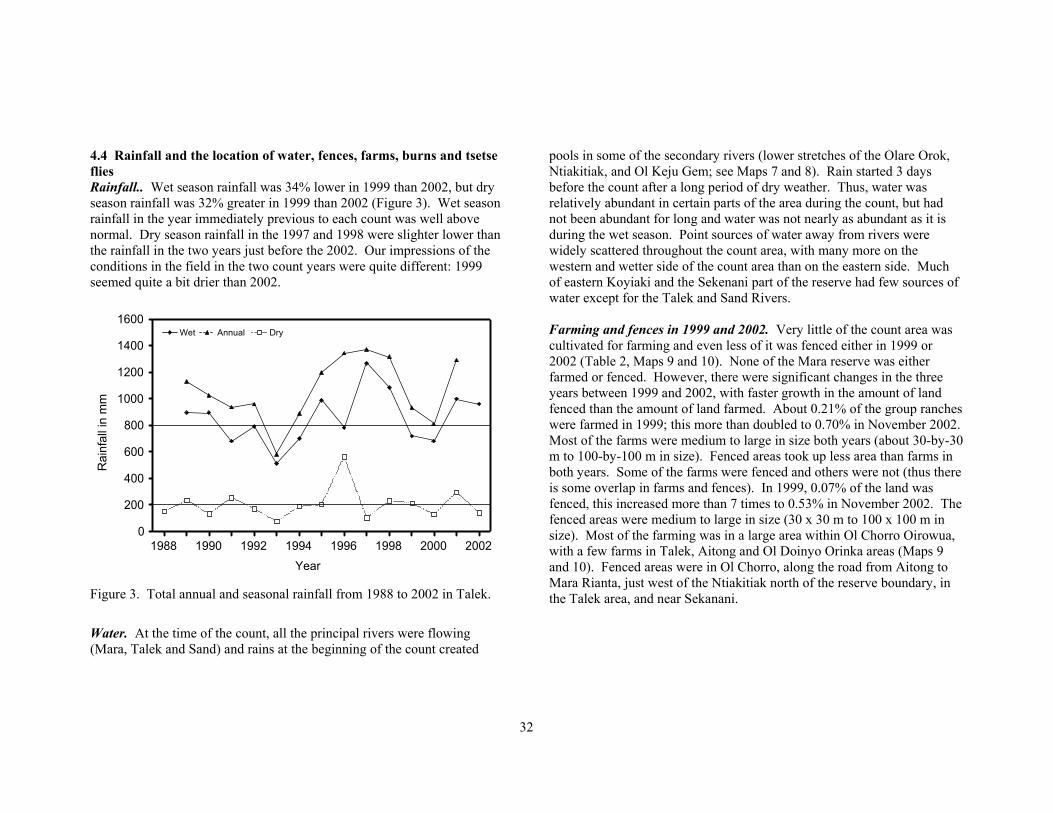
4.4 Rainfall and the location of water, fences, farms, burns and tsetse flies Rainfall.. Wet season rainfall was 34% lower in 1999 than 2002, but dry season rainfall was 32% greater in 1999 than 2002 (Figure 3). Wet season rainfall in the year immediately previous to each count was well above normal. Dry season rainfall in the 1997 and 1998 were slighter lower than the rainfall in the two years just before the 2002. Our impressions of the conditions in the field in the two count years were quite different: 1999 seemed quite a bit drier than 2002.

Year

Rai

nfal

l in

mm

0

200

400

600

800

1000

1200

1400

1600

1988 1990 1992 1994 1996 1998 2000 2002

Wet Annual Dry

Figure 3. Total annual and seasonal rainfall from 1988 to 2002 in Talek.

Water. At the time of the count, all the principal rivers were flowing (Mara, Talek and Sand) and rains at the beginning of the count created

pools in some of the secondary rivers (lower stretches of the Olare Orok, Ntiakitiak, and Ol Keju Gem; see Maps 7 and 8). Rain started 3 days before the count after a long period of dry weather. Thus, water was relatively abundant in certain parts of the area during the count, but had not been abundant for long and water was not nearly as abundant as it is during the wet season. Point sources of water away from rivers were widely scattered throughout the count area, with many more on the western and wetter side of the count area than on the eastern side. Much of eastern Koyiaki and the Sekenani part of the reserve had few sources of water except for the Talek and Sand Rivers. Farming and fences in 1999 and 2002. Very little of the count area was cultivated for farming and even less of it was fenced either in 1999 or 2002 (Table 2, Maps 9 and 10). None of the Mara reserve was either farmed or fenced. However, there were significant changes in the three years between 1999 and 2002, with faster growth in the amount of land fenced than the amount of land farmed. About 0.21% of the group ranches were farmed in 1999; this more than doubled to 0.70% in November 2002. Most of the farms were medium to large in size both years (about 30-by-30 m to 100-by-100 m in size). Fenced areas took up less area than farms in both years. Some of the farms were fenced and others were not (thus there is some overlap in farms and fences). In 1999, 0.07% of the land was fenced, this increased more than 7 times to 0.53% in November 2002. The fenced areas were medium to large in size (30 x 30 m to 100 x 100 m in size). Most of the farming was in a large area within Ol Chorro Oirowua, with a few farms in Talek, Aitong and Ol Doinyo Orinka areas (Maps 9 and 10). Fenced areas were in Ol Chorro, along the road from Aitong to Mara Rianta, just west of the Ntiakitiak north of the reserve boundary, in the Talek area, and near Sekanani.

33

Map 7. Sources of surface water in the count area between 9-16 November 2002, as recorded during aerial surveys.

34

Map 8. Sources of surface water as recorded by ground counting teams between 9-16 November, 2002.

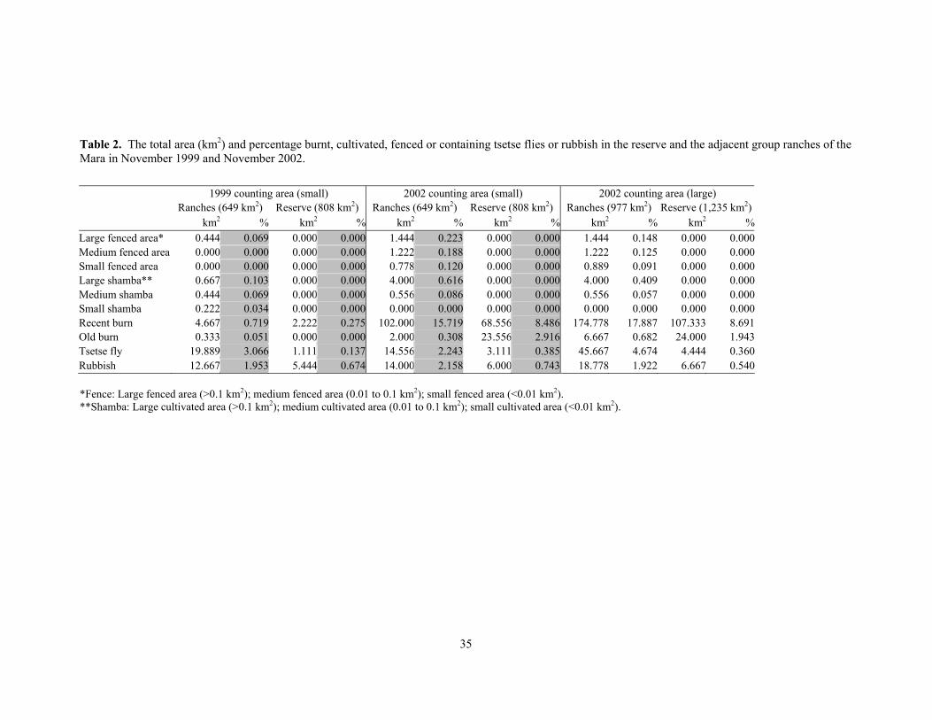
35

Table 2. The total area (km2) and percentage burnt, cultivated, fenced or containing tsetse flies or rubbish in the reserve and the adjacent group ranches of the Mara in November 1999 and November 2002.

1999 counting area (small) 2002 counting area (small) 2002 counting area (large) Ranches (649 km2) Reserve (808 km2) Ranches (649 km2) Reserve (808 km2) Ranches (977 km2) Reserve (1,235 km2) km2 % km2 % km2 % km2 % km2 % km2 %Large fenced area* 0.444 0.069 0.000 0.000 1.444 0.223 0.000 0.000 1.444 0.148 0.000 0.000Medium fenced area 0.000 0.000 0.000 0.000 1.222 0.188 0.000 0.000 1.222 0.125 0.000 0.000Small fenced area 0.000 0.000 0.000 0.000 0.778 0.120 0.000 0.000 0.889 0.091 0.000 0.000Large shamba** 0.667 0.103 0.000 0.000 4.000 0.616 0.000 0.000 4.000 0.409 0.000 0.000Medium shamba 0.444 0.069 0.000 0.000 0.556 0.086 0.000 0.000 0.556 0.057 0.000 0.000Small shamba 0.222 0.034 0.000 0.000 0.000 0.000 0.000 0.000 0.000 0.000 0.000 0.000Recent burn 4.667 0.719 2.222 0.275 102.000 15.719 68.556 8.486 174.778 17.887 107.333 8.691Old burn 0.333 0.051 0.000 0.000 2.000 0.308 23.556 2.916 6.667 0.682 24.000 1.943Tsetse fly 19.889 3.066 1.111 0.137 14.556 2.243 3.111 0.385 45.667 4.674 4.444 0.360Rubbish 12.667 1.953 5.444 0.674 14.000 2.158 6.000 0.743 18.778 1.922 6.667 0.540 *Fence: Large fenced area (>0.1 km2); medium fenced area (0.01 to 0.1 km2); small fenced area (<0.01 km2). **Shamba: Large cultivated area (>0.1 km2); medium cultivated area (0.01 to 0.1 km2); small cultivated area (<0.01 km2).

36

Burns. About 1.0 % of the count areas were burnt in 1999; this increased by 27 times to 27.4% in 2002 (Table 2, Map 11). The 1999 count took place in the middle of a long and severe drought, and thus there was probably little grass to burn in 1999. There was a bigger difference in the proportion of the group ranches and reserve burnt in 1999 than in 2002; 200% more land was burned on the group ranches than the reserve in 1999; in 2002, only 50% more savanna was burned in the ranches than reserve. Most of the burns occurred within 1-2 months of the beginning of each of the counts (there were no old burns in the reserve in 1999 at all). In 2002, burns were widely distributed on the group ranches, but restricted to particular areas in the reserve. The only two large areas that were not burned in the group ranches were a large area northwest of Aitong and in and south of Ol Doinyo Orinka. In the reserve, only the eastern and western parts of the Triangle were not burned, and the large area south of the Ol Keju Gem River. The only large older burn was in the Keekorok area inside the reserve. None of the burned areas overlapped with where there were high concentrations of bomas, but many of the large burns were within 1 km of groups of bomas. Tsetse flies. Our method of counting tsetse flies (we count flies only if we find them inside the vehicle) probably only measures the areas heavily infested with tsetse. Only a small part of either the group ranches or reserve were heavily infested either year; 2-3% of the group ranches were infested either year and 0.1-0.3% of the reserve were infested either year (Map 12, Table 2). However, the flies were much more common in the group ranches than in the reserve, infesting about 23 times as much area of land on the group ranches than in the reserve in 1999 and 5-6 times more in 2002. There are more flies in the group ranches probably because there is more wooded tsetse habitat here than in the reserve. Tsetse flies were also more common in 1999 than 2002 in the group ranch, but the opposite was true for the reserve. The area infested grew by almost 2 times in the group ranches from 1999 to 2002, but grew four times (twice as fast) in the

reserve from 1999 to 2002, probably because the 1999 drought reduced the number of flies. Flies were most common in southeastern Koyiaki and just to the west of the Talek-Aitong road; these areas have the best tsetse habitat (see shrub and tree cover, Maps 20 and 23). We also found flies in an area on the mid-western edge of the Triangle near the Siria Escarpment. Most of the flies were in large patches that covered 10’s of square km. As expected, people rarely established bomas in these tsetse belts. There were also few tourist lodges where there were tsetse flies! This is true even though some of the largest, multiple species associations of wildlife are found in the tsetse-infested areas. 4.5 Location of tourist lodges, other infrastructure, vehicles and rubbish Lodges and other infrastructure. Nearly all the lodges were built along permanent water courses, with the exception of some mobile tented camps (Map 13). Most of the lodges are within the reserve or clustered along the Talek River near Talek village. There are 10 schools in the counting area, 4 football pitches, 13 airstrips, 72 tourist lodges and camps, 7 veterinary dips, 10 cattle crushes, and 69 shops (Map 14 of other infrastructure). Rubbish. Even though we found rubbish in a small part of the count area, it was often common where we found it. Most of the rubbish was in the form of plastic bags. About 75% of the rubbish was in the group ranches, with 25% in the reserve. However, even on the group ranches, we found rubbish only in one of every 50 sub-blocks (2% of sub-blocks) we counted (see Table 2 above). Most of the rubbish was in town centers or around bomas in the group ranches, but the rubbish (probably left by tourists) was near roads in the reserve (Map 15). The amount of area covered with rubbish in the group ranches and the reserve did not change between 1999 and 2002 (see % figures in Table 2).

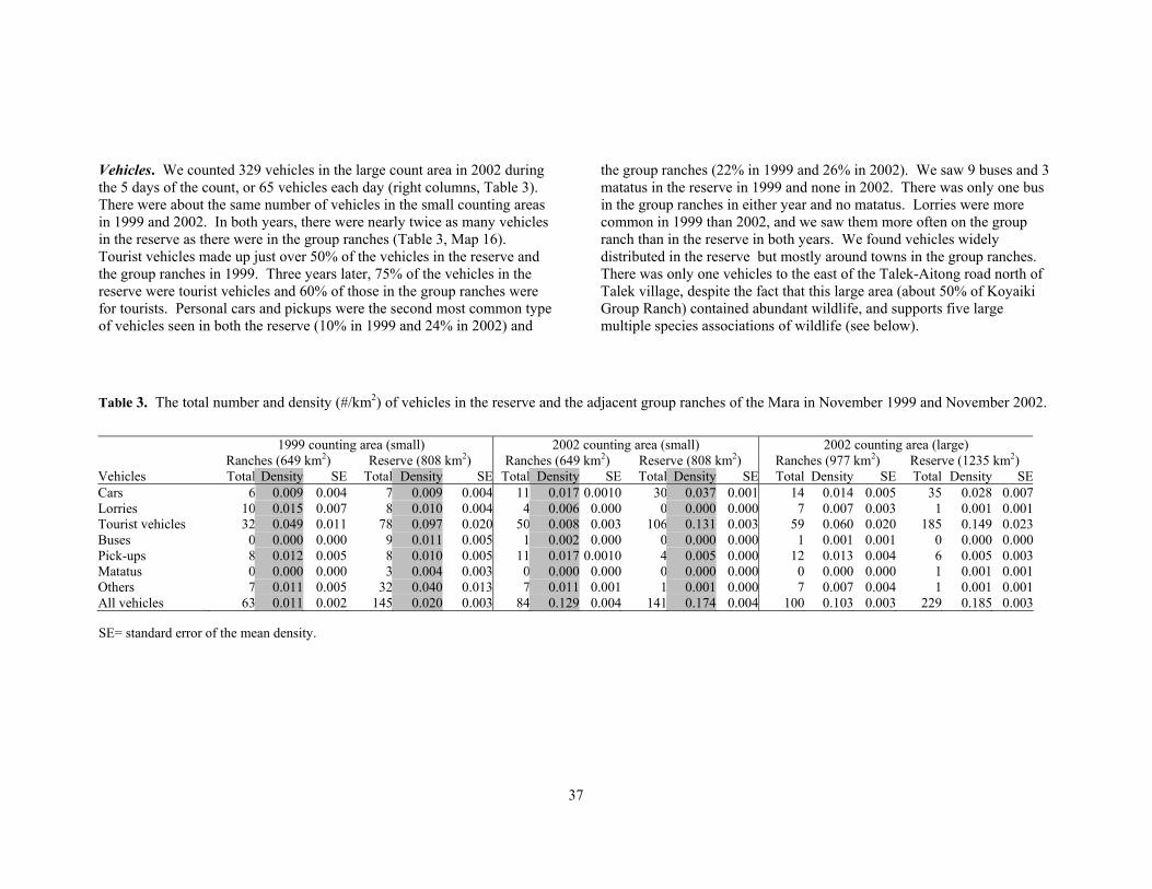
37

Vehicles. We counted 329 vehicles in the large count area in 2002 during the 5 days of the count, or 65 vehicles each day (right columns, Table 3). There were about the same number of vehicles in the small counting areas in 1999 and 2002. In both years, there were nearly twice as many vehicles in the reserve as there were in the group ranches (Table 3, Map 16). Tourist vehicles made up just over 50% of the vehicles in the reserve and the group ranches in 1999. Three years later, 75% of the vehicles in the reserve were tourist vehicles and 60% of those in the group ranches were for tourists. Personal cars and pickups were the second most common type of vehicles seen in both the reserve (10% in 1999 and 24% in 2002) and

the group ranches (22% in 1999 and 26% in 2002). We saw 9 buses and 3 matatus in the reserve in 1999 and none in 2002. There was only one bus in the group ranches in either year and no matatus. Lorries were more common in 1999 than 2002, and we saw them more often on the group ranch than in the reserve in both years. We found vehicles widely distributed in the reserve but mostly around towns in the group ranches. There was only one vehicles to the east of the Talek-Aitong road north of Talek village, despite the fact that this large area (about 50% of Koyaiki Group Ranch) contained abundant wildlife, and supports five large multiple species associations of wildlife (see below).

Table 3. The total number and density (#/km2) of vehicles in the reserve and the adjacent group ranches of the Mara in November 1999 and November 2002.

1999 counting area (small) 2002 counting area (small) 2002 counting area (large) Ranches (649 km2) Reserve (808 km2) Ranches (649 km2) Reserve (808 km2) Ranches (977 km2) Reserve (1235 km2) Vehicles Total Density SE Total Density SE Total Density SE Total Density SE Total Density SE Total Density SECars 6 0.009 0.004 7 0.009 0.004 11 0.017 0.0010 30 0.037 0.001 14 0.014 0.005 35 0.028 0.007Lorries 10 0.015 0.007 8 0.010 0.004 4 0.006 0.000 0 0.000 0.000 7 0.007 0.003 1 0.001 0.001Tourist vehicles 32 0.049 0.011 78 0.097 0.020 50 0.008 0.003 106 0.131 0.003 59 0.060 0.020 185 0.149 0.023Buses 0 0.000 0.000 9 0.011 0.005 1 0.002 0.000 0 0.000 0.000 1 0.001 0.001 0 0.000 0.000Pick-ups 8 0.012 0.005 8 0.010 0.005 11 0.017 0.0010 4 0.005 0.000 12 0.013 0.004 6 0.005 0.003Matatus 0 0.000 0.000 3 0.004 0.003 0 0.000 0.000 0 0.000 0.000 0 0.000 0.000 1 0.001 0.001Others 7 0.011 0.005 32 0.040 0.013 7 0.011 0.001 1 0.001 0.000 7 0.007 0.004 1 0.001 0.001All vehicles 63 0.011 0.002 145 0.020 0.003 84 0.129 0.004 141 0.174 0.004 100 0.103 0.003 229 0.185 0.003 SE= standard error of the mean density.

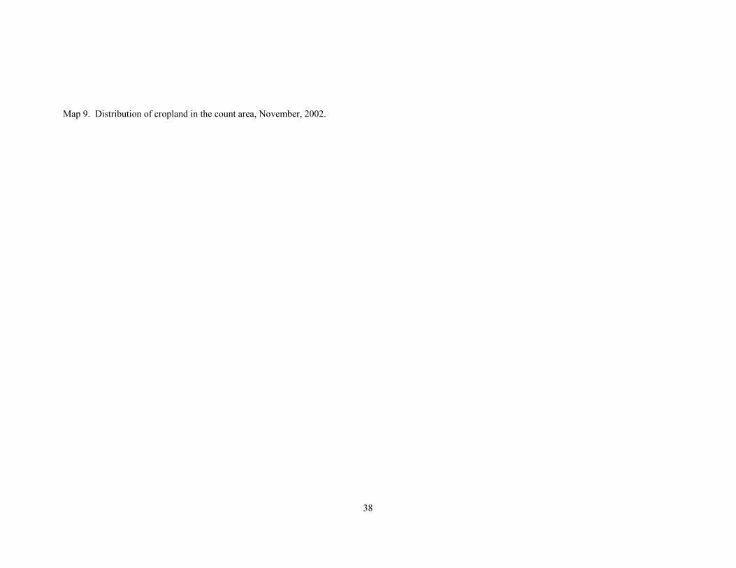
38

Map 9. Distribution of cropland in the count area, November, 2002.

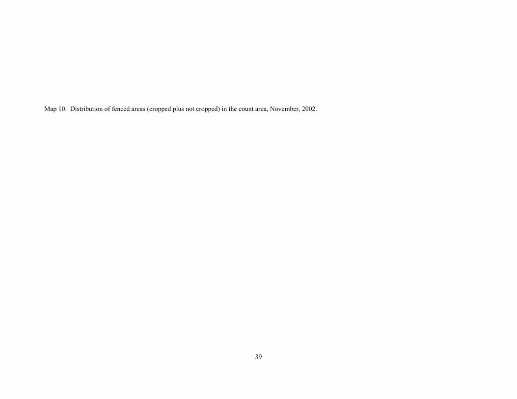
39

Map 10. Distribution of fenced areas (cropped plus not cropped) in the count area, November, 2002.

40

Map 11. Areas burned by bush fires at different times before the count.

41

Map 12. Distribution of tsetse flies in the count area, November, 2002.

42

Map 13. Distribution and types of tourist lodges in the count area, November, 2002.

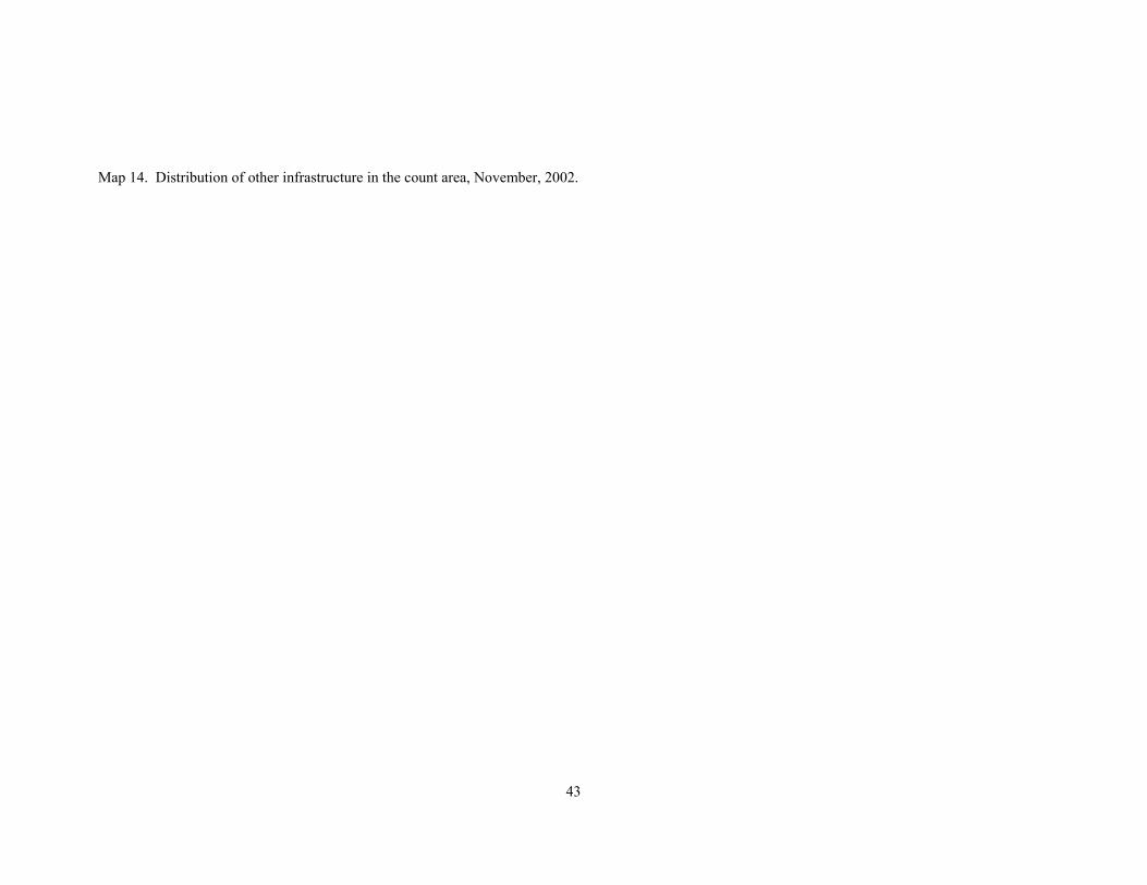
43

Map 14. Distribution of other infrastructure in the count area, November, 2002.

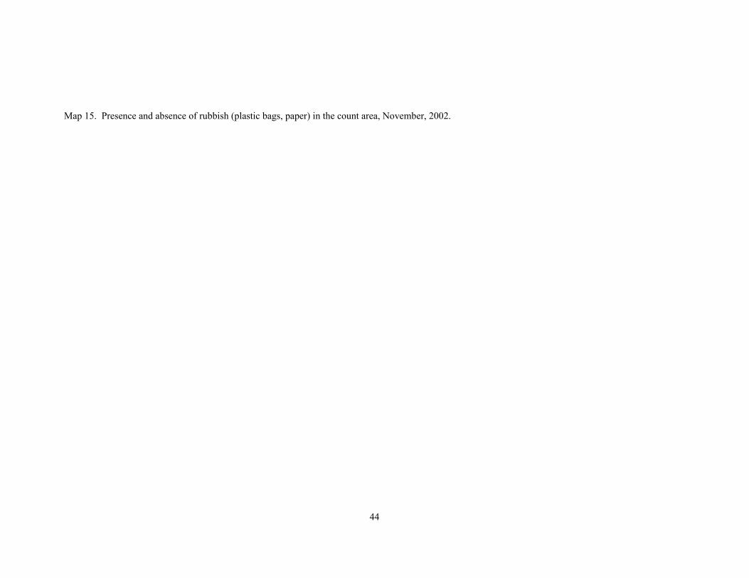
44

Map 15. Presence and absence of rubbish (plastic bags, paper) in the count area, November, 2002.

45

Map 16. Distribution of motor vehicles during the count in November, 2002.

46

4.6 Height, amount (cover) and colour of grass, trees and shrubs How much grass? The percentage grass cover14 measures how much of the ground’s surface is covered by live grass, regardless of the colour or height of the grass. Grass tends to cover more ground where the soil is wetter and grass is more productive (around rivers, swamps and floodplains), where it has not burned or where animal grazing is low. A loss in grass cover can be an indication of degradation, but not always (for example, burned areas often have low grass cover right after a burn, but this does not usually mean the areas is degraded). Grass cover was greater in the reserve (71-73% cover) in both years than the group ranches (60-63% cover, Table 4). Many of the areas with high grass cover in 2002 were also areas that had not been recently burned (compare Maps 11 and 17). In 2002, there were pockets of high grass cover in the group ranches (near Mara Rianta and to the northeast of the Talek). The grass in these areas was also very tall (Map 18). There were large areas of very high grass cover and tall grass in the reserve, in the northern and central Triangle and west of Keekorok in an area spanning the Ol Keju Gem River, north and south. Grass cover was very low (blue and green on Map 17) in the western Triangle, in Talek, and around Ol Doinyo Orinka, and along the Ntiakitiak River. How tall was the grass? In the Mara, the height of the grass seems to be a good indication of how much an area has been grazed recently; it can also indicate areas that were burned recently. In 1999, grass in the reserve (17 cm tall) was nearly 50% taller than that in the group ranches (11.5 cm tall). In 2002, there was no appreciable difference in grass heights (about 13-14 cm tall) in the reserve and group ranches. Outside the reserve, grass was short near clusters of bomas or villages like Talek where livestock grazing 14 We measured aerial plant cover (cover of all above ground parts of the plant including all stems, branches and leaves) rather than basal plant cover (cover of just the base of the plant). The former is strongly affected by burning and grazing; the latter often is not affected by burning or grazing.

is heavy and there was significant burning (Map 18). Mixed with these low grass areas near bomas were many high grass areas that are probably places where the Maasai avoid grazing near bomas as a reserve of forage for their calves in the dry season (an olekeri). During interviews in June 2003, Maasai informants in the Olare Orok areas said they often place their grazing reserves near rivers. Inside the reserve, we found short grass in the western corner of the Triangle (where we also found the wildebeest migration), in central Musiara (burning and cattle grazing), and in the southeast near the Sand River. Grass was particularly tall in and southwest of Ol Chorro Oirowua, in places that were far from bomas, south of Mara Rianta and in the northern Triangle, northeast of Talek and in the Ol Keju Gem area. How green was the grass? Grass was greenest either where it had burned and rained recently or where it had been grazed and rained recently. The grass was much greener in 2002 (37-62% green) than in 1999 (19-23% green, Table 4). Grass was greener in the reserve than in the group ranches in both years, and this difference was most pronounced in 2002 (21% relative difference in 1999 and 71% difference in 2002). In general, grass was greener to the south and the west of the count area than to the north and east (Map 19). During the count, it rained first by the Siria escarpment and last near Ol Doinyo Orinka. In the dry area to the northeast of Talek, grass was only green where it had burned recently. In the wetter areas to the west, areas that had been grazed heavily and burned were green. The areas with the brownest grass were places where there had been no burning and no rain. How much green grass was there? We calculated two simple indices of the amount of grass (green or not) available for grazers and the amount of green grass available (Table 4). The first index of available grass gives an estimate of the amount of grass available for wildlife species that do not have to have green grass (they will eat green and non-green grass), like

47

elephants, buffalo, and zebra. The numbers show that, in both years, there was more grass available for these grazers in the reserve. Interestingly, the difference between the reserve and group ranches was more pronounced in 1999 (75% difference) than 2002 (25% difference). Thus, these species, if attracted to amount of grass available, should be attracted to graze in the reserve more than the group ranches, and to a greater degree in 1999 than 2002. When we look at the green grass biomass, it is clear that, in both years, there was more than twice as much green grass biomass in the reserve than group ranches. Also, there was more than twice as much green grass biomass in 2002 than 1999. This provided all grazers that depend on green grass a strong reason to graze in the reserve in preference to the group ranches in both years. It also implies that the ecosystem could support more grazers altogether in November, 2002, than November, 1999. Shrubs. For this count, we defined shrubs as woody plants that are less than about 2 meters tall or have a shrubby growth form. The group ranches support 7.5% (40% in a relative sense) more shrub cover than the reserve (18.6% compared with 11.1%) in 1999 but there was no difference between the two areas in 2002 (10.7% compared with 9.0%, Table 4). Our shrub and tree cover estimates are difficult to make and thus are approximations, so we interpret the differences between 1999 and 2002 in shrub cover as possible sampling error due to different observers. The areas with the most shrubs were along the Mara River in the reserve and in northern Koyiaki, in the Olkinyei area northeast of Talek (Map 20). Shrub cover is noticeably low in the reserve with many areas with no shrubs, particularly in the southern part of Musiara and Sekanani sectors. Average shrub height in the group ranches and reserve was about 1.1-1.4 meters in both years. Our shrub height measurements are more reliable than the cover measurements, thus the slightly taller shrubs in 2002 may reflect regrowth of shrubs after the 1999-2000 drought. Shrubs were

particularly tall where the grass was tall in the northern Triangle, Ol Keju Gem area, Olkinyei area northeast of Talek and in the north along the Mara River (Map 21). Many of these areas have significant clumps of Euclea divinorum and ant gall acacia (Acacia drepanolobium). Shrubs were short in the west, in the Triangle, and north and west of the Ntiakitiak River. Shrub leaves were greener in 1999 than 2002 and also greener in the group ranches (75.4% green in 1999) than the reserve (60.3%), but only in 1999. Shrubs were noticeably green (Map 22) in the western Triangle, east of the Olare Orok River and in the Aitong area. Shrubs were brown where it had not rained in the Olkinyei area northeast of Talek and around Ol Doinyo Orinka. Trees. There are very few trees in all of the Mara. In both years, tree cover was less than 4% in the reserve, with 3 times more cover in the group ranches (11-12% cover) than the reserve. Most of the trees are in the patch of Acacia gerrardii woodland (infested with tsetse) surrounding the upper Ntiakitiak River, in the Olkinyei area northeast of Talek, along the Mara River and near Keekorok (Map 23). The average tree was 5.1 m tall in 1999 and 4.3-4.6 m tall in 2002. There was no significant difference in tree height between the reserve and group ranches in either year. The tallest trees are also where the shrubs and grass are tall in the northern and central Triangle, around and south of the Ol Keju Gem, in the hills above Talek and in Ol Chorro Oirowua (Map 24). Trees were greener in 1999 than 2002, and greener in the group ranches than in the reserve. Trees were greener than shrubs, which, in turn, were greener than grasses. In the dry season (which is when we counted), trees and shrubs are often greener than grass because they have deeper roots and access to deeper underground water. Tree colour was reasonably uniform throughout the Mara (Map 25).

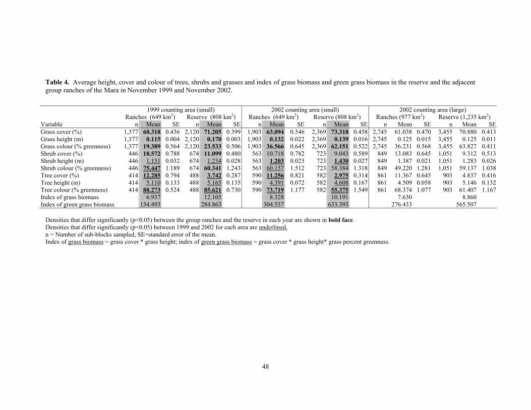
48

Table 4. Average height, cover and colour of trees, shrubs and grasses and index of grass biomass and green grass biomass in the reserve and the adjacent group ranches of the Mara in November 1999 and November 2002.

1999 counting area (small) 2002 counting area (small) 2002 counting area (large)

Ranches (649 km2) Reserve (808 km2) Ranches (649 km2) Reserve (808 km2) Ranches (977 km2) Reserve (1,235 km2) Variable n Mean SE n Mean SE n Mean SE n Mean SE n Mean SE n Mean SE Grass cover (%) 1,377 60.318 0.436 2,120 71.205 0.399 1,903 63.094 0.546 2,369 73.318 0.458 2,745 61.038 0.470 3,455 70.880 0.413 Grass height (m) 1,377 0.115 0.004 2,120 0.170 0.003 1,903 0.132 0.022 2,369 0.139 0.016 2,745 0.125 0.015 3,455 0.125 0.011 Grass colour (% greenness) 1,377 19.389 0.564 2,120 23.533 0.506 1,903 36.566 0.645 2,369 62.151 0.522 2,745 36.231 0.568 3,455 63.827 0.411 Shrub cover (%) 446 18.572 0.788 674 11.099 0.480 563 10.718 0.782 723 9.043 0.589 849 13.083 0.645 1,051 9.312 0.513 Shrub height (m) 446 1.151 0.032 674 1.234 0.028 563 1.203 0.023 723 1.430 0.027 849 1.387 0.021 1,051 1.283 0.026 Shrub colour (% greenness) 446 75.447 1.189 674 60.341 1.243 563 60.157 1.512 723 58.384 1.318 849 49.220 1.281 1,051 59.137 1.038 Tree cover (%) 414 12.285 0.794 488 3.742 0.287 590 11.256 0.821 582 2.975 0.314 861 11.367 0.645 903 4.837 0.416 Tree height (m) 414 5.110 0.133 488 5.165 0.135 590 4.391 0.072 582 4.608 0.167 861 4.509 0.058 903 5.146 0.132 Tree colour (% greenness) 414 88.273 0.524 488 85.621 0.730 590 73.719 1.177 582 55.375 1.549 861 68.374 1.077 903 61.407 1.167 Index of grass biomass 6.937 12.105 8.328 10.191 7.630 8.860 Index of green grass biomass 134.493 284.863 304.537 633.393 276.433 565.507

Densities that differ significantly (p<0.05) between the group ranches and the reserve in each year are shown in bold face. Densities that differ significantly (p<0.05) between 1999 and 2002 for each area are underlined. n = Number of sub-blocks sampled, SE=standard error of the mean. Index of grass biomass = grass cover * grass height; index of green grass biomass = grass cover * grass height* grass percent greenness.

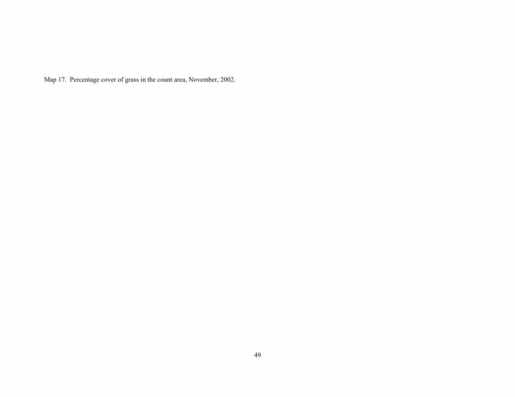
49

Map 17. Percentage cover of grass in the count area, November, 2002.

50

Map 18. Height of grass (in centimeters) at block level (1km2) in the count area, November, 2002.

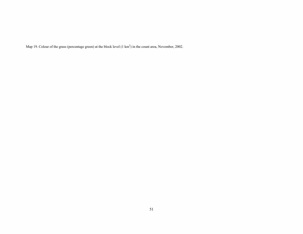
51

Map 19. Colour of the grass (percentage green) at the block level (1 km2) in the count area, November, 2002.

52

Map 20. Percentage of ground covered by shrubs at block level (1 km2) in the count area, November, 2002.

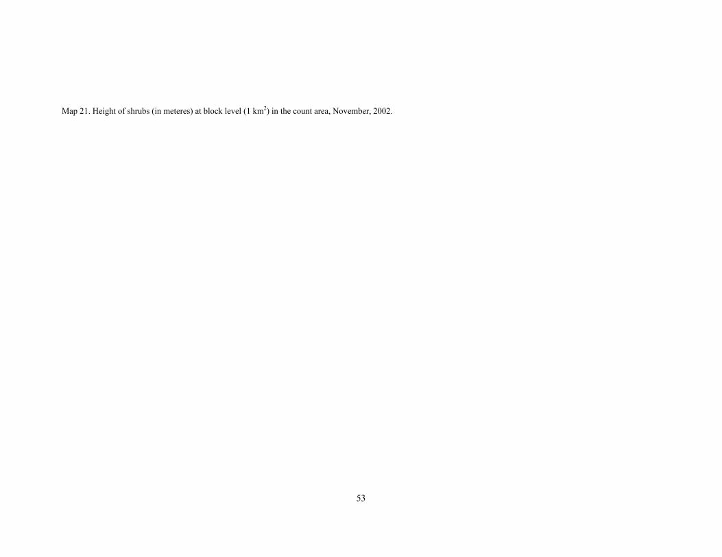
53

Map 21. Height of shrubs (in meteres) at block level (1 km2) in the count area, November, 2002.

54

Map 22. Colour of shrub leaves (percentage green) at block level (1 km2) in the count area, November, 2002.

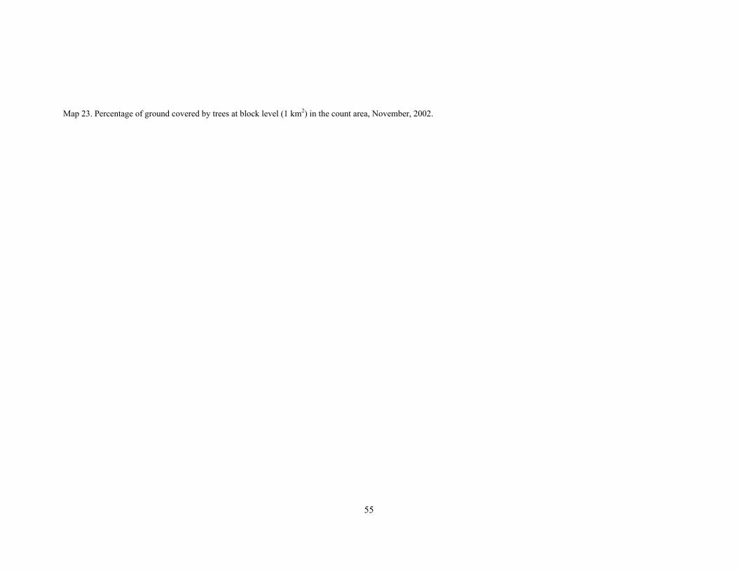
55

Map 23. Percentage of ground covered by trees at block level (1 km2) in the count area, November, 2002.

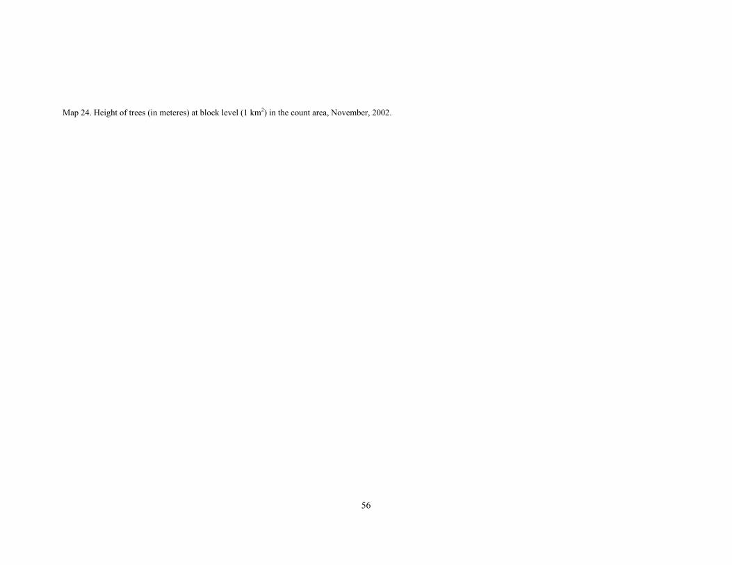
56

Map 24. Height of trees (in meteres) at block level (1 km2) in the count area, November, 2002.

57

Map 25. Colour of tree leaves (percentage green) at block level (1 km2) in the count area, November, 2002.

58

4.7 Livestock: how many and where? As we expected, there were many more cattle, sheep, goats15, donkeys and dogs in the group ranches than in the reserve in both 1999 and 2002 (Tables 5 and 6). However, a large part of the cattle herd that we counted was in the reserve during the count in 1999 and this proportion grew larger by 2002. In 1999, about a quarter (24%) of all the cattle we counted were in the reserve (and 76% in the group ranch). In 2002, we found more than a third (36%) of the cattle in reserve and two-thirds (63%) in the group ranch. In real numbers, this represents a doubling in the number of cattle in the reserve between 1999 and 2002 (from 10,920 to 22,257 cattle). Most of the cattle were in the Musiara sector (20.6 cattle/km2), with about 70% as many animals as the Sekanani sector (13.9 animals/km2) and very few in the Triangle (1.0 cattle/km2, Appendix Table A4). We found many fewer sheep and goats in the reserve in 1999 (8% of the herd or 1704 shoats) than 2002 (16% of the herd or 7,426 shoats). Like cattle, most of the shoats were found in the Musiara area and the fewest in the Triangle. In terms of biomass, and thus use of forage, cattle biomass in the reserve outweighed that of shoats by as much as 20:1 in 2002 (Table 6 and Appendix Table A5). In absolute numbers, there was more than a 330% increase in the number of shoats in the reserve from 1999 to 2002. We found very few dogs or donkeys in the reserve either year (2-4%, 3-13 animals). Between 1976 and 1996, cattle numbers on Koyiaki Group Ranch have varied between 20,000 and 45,000, depending strongly on the rainfall received over the previous two years, with no marked long-term increase 16. R. Lamprey describes this variation in livestock numbers on Koyiaki Group Ranch from year to year as follows:

15 We counted sheep and goats together in the count because they are difficult to distinguish when herded in tightly packed groups. We will often use the term ‘shoats’ to refer to them together here. 16 Broten and Said 1995, Serneels and Lambin 2001, Lamprey and Reid submitted

‘Livestock estimates for Koyake reflect the general trend for all Mara ranches. The Koyake cattle population increased to about 40,000 head in the late 1980s, following good rainfall and increased primary production. In the early 90’s, poor rainfall resulted in a decline to about 25,000 head. A further period of good rainfall in 1997/98, associated with ‘El Nino’, led to an increase again to 40,000; this was followed by a massive 'crash' in the catastrophic ‘La Nina’ drought of 1999/2000…’

In the middle of this ‘crash’, we counted cattle on Koyiaki in November 1999 and cattle numbers had fallen to about 16,300. Our ground counts in 2002 showed that cattle populations recovered rapidly again, with an estimated 33,300 head on Koyiaki. On a per person basis, there was also an increase between 1999 and 2002. The Maasai of the Mara need an estimated 1125-1575 (average = 1350 kg) kg liveweight of livestock per person (there is some difference in estimates of this requirement from author to author17) to rely completely on livestock for subsistence. These come mainly from cattle and sheep and goats. In 1999, there were a total of 283 kg of cattle/person available in our count area and 59 kg of shoats/person, for a total of 335 kg/person or 335/1350 required, only 25% (335 kg/1350 kg required) of their needs. In 2002, this rose to 37% with 497 kg/person available. The Maasai of the Mara find themselves in a position similar to those in Ngorongoro where the amount of liveweight available per person has decreased by 60% between 1987 and 199818, with only about 50% of the Maasai requirements met by livestock in 1998.

17 Brown 1971, Pratt and Gwynne 1977, Jewell 1980, Bekure and others 1971, Kjaerby in Homewood and Rodgers 1991 18See Homewood and Rodgers 1991; McCabe and others 1997, and NCAA 1999

59

For the Mara Maasai, some 65-75% of their requirements must come options other than livestock. There are a range of options available, depending on whether the household is near wildlife-rich areas like the reserve or near agricultural markets19. Different income alternatives include cultivation of crops, consumptive use of wildlife, cultivation leases, remittances from family members now living in the cities, employment in lodges, revenues from 'cultural manyattas', and the receipt of small tourism ‘dividends’ from wildlife associations. This explains the pressure for pastoralists to expand livestock grazing into the reserve. Cattle, sheep and goat populations doubled in the three years between 1999 and 2002 (Table 5 and 6). Our Maasai team members say that many of the cattle were being herded outside of the Mara group ranches in 1999 because of the drought. Thus, some of the increase between the two years is from reproduction, some from purchase of new cattle and some from the return of cattle that were being herded elsewhere. The ratio of shoats: cattle in the drought year of 1999 was 1.85 : 1 and in the wetter year of 2002, it was marginally lower at 1.80 : 1. R. Lamprey describes sheep and goat populations as follows:

‘Over the 1990’s the Maasai have increased their sheep and goat herds, usually a strategy in times of drought or hardship20 (Grandin 1988; Homewood and Rodgers 1991). The contribution of sheep and goats to total livestock biomass increased from 7.1% in 1979 to 9.9% in the late 1990s. With current trends this proportion may increase further.’

Donkey populations fell by half on the group ranches between 1999 and 2002. Domestic dog populations grew by about 123% on the group ranches between the two counts. 19 Homewood and others 2001; Thompson and Homewood 2002 20 Grandin 1988, Homewood and Rodgers 1991

In 2002, we found cattle mostly around Talek, the Olare Orok area, Ol Doinyo Orinka, northwest of Aitong and at Mara Rianta (Map 26). The largest herds were near Aitong and in the Mara reserve (> 200 cattle per herd). Very few cattle were in the Triangle part of the reserve during the count (1/km2); more were in the Sekanani section (14/km2) with the most the Musiara section (21/km2). Smaller herds of cattle were nearly everywhere on the group ranches except in those areas with significant tsetse flies (see Map 12). We found cattle both near and far from water and both near and far from bomas. Sheep and goats stayed close to bomas and thus were clustered around village centers or groups of bomas (Map 27). We found large concentrations of these ‘shoats’ near Aitong, Ol Doinyo Orinka, Talek, Mara Rianta, Sekanani and between the Olare Orok and Ntiakitiak Rivers just north of the reserve. Few shoats were grazing inside the reserve, except in the northern Triangle and around the Olare Orok. There were few sheep and goats where there were tsetse flies. There were few donkeys in the counting area, and all of them were near a boma (Map 28). Dogs ranged farther from bomas, often with the sheep and goats (Map 29). We counted 7 donkeys in the reserve and a few dogs in 2002, some well within the reserve boundaries. Altogether, livestock were concentrated in two bands at the edge and north of the Mara reserve (Map 30). One band stretches from Sekanani to Talek and another from Ol Doinyo Orinka to Aitong and beyond to the Mara River. These two bands are separated by an area with very few or no livestock that is infested with tsetse flies.

60

Table 5. Total numbers, densities (animals per km2) and standard errors (SE) of livestock and wildlife in the reserve and the adjacent group ranches of the Mara in November 1999 and November 2002.

1999 counting area (small) 2002 counting area (small) 2002 counting area (large) Ranches (649 km2) Reserve (808 km2) Ranches (649 km2) Reserve (808 km2) Ranches (977 km2) Reserve (1,235 km2)

Species Total Density SE Total Density SE Total Density SE Total Density SE Total Density SE Total Density SECattle 10,920 16.835 2.157 3,445 4.076 1.142 22,257 34.299 3.251 12,910 15.984 2.861 31,683 32.425 2.522 13,350 10.808 1.883Donkey 375 0.578 0.120 11 0.013 0.012 168 0.261 0.063 7 0.009 0.009 296 0.303 0.054 7 0.005 0.005Sheep & goats 20,289 31.278 2.912 1,704 2.016 0.614 40,200 61.956 4.831 7,426 9.189 2.136 51,808 53.022 3.646 7,886 6.385 1.413Domestic dog 96 0.148 0.023 3 0.004 0.003 214 0.330 0.037 13 0.018 0.006 327 0.335 0.032 22 0.018 0.006Baboon 229 0.353 0.112 275 0.346 0.104 636 0.981 0.277 696 0.864 0.160 838 0.858 0.196 857 0.694 0.115Bat-eared fox (H) 6 0.009 0.005 12 0.014 0.007 12 0.018 0.008 8 0.009 0.005 20 0.021 0.007 19 0.015 0.005Buffalo (H) 325 0.501 0.243 1,073 1.271 0.458 50 0.081 0.053 1,053 1.305 0.488 96 0.098 0.055 2,465 1.995 0.492Bushbuck (H) 0 0.000 0.000 3 0.004 0.003 3 0.009 0.003 16 0.018 0.009 8 0.008 0.004 57 0.046 0.033Cheetah (H) 6 0.009 0.005 5 0.006 0.004 4 0.009 0.004 11 0.018 0.008 4 0.005 0.003 13 0.011 0.005Crocodile (H) 3 0.005 0.003 34 0.052 0.017 1 0.000 0.002 15 0.018 0.008 1 0.001 0.001 15 0.012 0.005Dikdik (H) 25 0.039 0.011 7 0.008 0.005 68 0.108 0.018 8 0.009 0.004 226 0.231 0.023 14 0.012 0.005Duiker (H) 0 0.000 0.000 1 0.001 0.001 3 0.009 0.003 5 0.009 0.003 3 0.003 0.002 6 0.005 0.002Eland 127 0.196 0.072 837 1.003 0.281 101 0.153 0.068 1,104 1.368 0.264 125 0.128 0.050 1,320 1.068 0.182Elephant 45 0.069 0.029 461 0.557 0.095 57 0.090 0.045 447 0.549 0.114 128 0.131 0.041 692 0.560 0.101Giraffe 384 0.592 0.098 199 0.240 0.049 421 0.648 0.086 200 0.252 0.049 566 0.580 0.068 314 0.254 0.046Grant's gazelle 1,087 1.676 0.257 1,276 1.521 0.137 1,273 1.962 0.174 2,194 2.718 0.203 2,547 2.606 0.173 2,369 1.918 0.162Hare (S) 1 0.002 0.002 2 0.002 0.002 10 0.015 0.005 12 0.015 0.005 38 0.039 0.007 12 0.010 0.004Hartebeest 93 0.143 0.039 320 0.379 0.075 108 0.162 0.050 339 0.423 0.073 192 0.196 0.041 425 0.344 0.054Hippopotamus (H) 61 0.094 0.059 480 0.598 0.191 76 0.117 0.070 334 0.414 0.150 120 0.122 0.058 395 0.320 0.107Honey badger (S) 0 0.000 0.000 1 0.001 0.001 1 0.002 0.002 24 0.030 0.018 1 0.001 0.001 24 0.020 0.012Hyena (H) 43 0.066 0.023 82 0.097 0.022 64 0.099 0.024 139 0.171 0.028 84 0.086 0.017 167 0.135 0.019Impala 5,995 9.242 0.826 3,775 4.485 0.452 7,928 12.222 0.898 4,907 6.075 0.464 12,709 13.007 0.779 6,928 5.609 0.374Jackal (H) 17 0.026 0.009 17 0.020 0.007 44 0.072 0.014 71 0.090 0.016 70 0.072 0.013 89 0.072 0.012Leopard (H) 0 0.000 0.000 2 0.002 0.002 0 0.000 0.000 1 0.000 0.001 1 0.001 0.001 1 0.001 0.001Lion (H) 4 0.006 0.005 42 0.051 0.023 37 0.054 0.033 111 0.135 0.039 46 0.047 0.023 123 0.100 0.026Mongoose (S) 65 0.100 0.048 60 0.074 0.029 274 0.422 0.088 477 0.590 0.099 362 0.371 0.065 726 0.588 0.082Oribi 0 0.000 0.000 0 0.000 0.000 0 0.000 0.000 0 0.000 0.000 0 0.000 0.000 122 0.011 0.002Ostrich 18 0.028 0.012 142 0.168 0.034 58 0.090 0.038 238 0.297 0.098 83 0.085 0.026 256 0.207 0.065Reedbuck (H) 0 0.000 0.000 27 0.033 0.009 0 0.000 0.000 143 0.180 0.024 0 0.000 0.000 200 0.162 0.019Rhinoceros (H) 0 0.000 0.000 1 0.001 0.001 1 0.000 0.002 10 0.009 0.008 1 0.001 0.001 10 0.008 0.005Thomson's gazelle 10,359 15.970 0.832 13,859 16.703 0.765 18,256 28.134 1.509 17,210 21.303 0.933 24,134 24.700 1.124 26,599 21.533 0.787Topi 1,735 2.675 0.239 3,699 4.379 0.360 2,456 3.789 0.244 3,402 4.212 0.290 3,156 3.230 0.178 4,545 3.679 0.227Tortoise (S) 0 0.000 0.000 1 0.001 0.001 9 0.018 0.005 30 0.036 0.008 21 0.022 0.005 33 0.027 0.005Vervet monkey (H) 123 0.190 0.066 12 0.014 0.007 145 0.225 0.073 142 0.180 0.098 229 0.234 0.059 193 0.157 0.068Vulture (H) 73 0.113 0.047 585 0.724 0.193 167 0.257 0.055 712 0.881 0.151 296 0.303 0.070 1,052 0.851 0.117Warthog 323 0.498 0.065 671 0.832 0.087 479 0.738 0.069 1,110 1.377 0.090 608 0.622 0.050 1,661 1.345 0.074Waterbuck 161 0.248 0.087 275 0.338 0.119 229 0.351 0.077 220 0.270 0.050 253 0.259 0.053 483 0.391 0.062Wildebeest 8,268 12.746 1.182 62,036 79.209 9.004 16,597 25.578 1.805 87,535 108.351 8.829 19,083 19.532 1.263 135,002 109.293 6.270Zebra 5,122 7.896 0.575 9,936 11.951 1.085 10,254 15.804 1.088 16,967 21.006 1.652 11,641 11.913 0.743 27,317 22.115 1.225Densities that differ significantly (p<0.05) between the group ranches and the reserve in each year are shown in bold face. Densities that differ significantly (p<0.05) between 1999 and 2002 for each area are underlined.(S)=species difficult to count because they are small in size; (H)=Species that are difficult to count because they hide, inhabit bush or water.

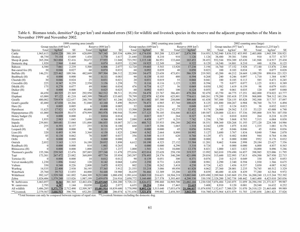
61

Table 6. Biomass totals, densities* (kg per km2) and standard errors (SE) for wildlife and livestock species in the reserve and the adjacent group ranches of the Mara in November 1999 and November 2002.

1999 counting area (small) 2002 counting area (small) 2002 counting area (large) Group ranches (649 km2) Reserve (808 km2) Group ranches (649 km2) Reserve (808 km2) Group ranches (977 km2) Reserve (1,235 km2)

Species Total kg/km2 SE Total kg/km2 SE Total kg/km2 SE Total kg/km2 SE Total kg/km2 SE Total kg/km2 SE Cattle 1,965,613 3,030.220 388.189 620,099 767.345 205.554 4,006,205 6,174.030 585.208 2,323,807 2,876.390 514.951 5,702,940 5,836.532 453.995 2,403,000 1,945.399 338.921 Donkey 48,750 75.154 15.609 1,430 1.770 1.617 21,840 33.658 8.210 910 1.126 1.126 38,480 39.381 7.056 910 0.737 0.737 Sheep & goats 365,204 563.004 52.416 30,672 37.955 11.048 723,592 1,115.140 86.951 133,668 165.453 38.453 932,544 954.389 65.630 141,948 114.917 25.430 Domestic dog 1,920 2.960 0.460 60 0.074 0.055 12,280 18.925 12.349 260 0.322 0.129 14,540 14.881 8.210 440 0.356 0.125 Baboon 4,580 7.061 2.239 5,500 6.806 2.077 12,720 19.603 5.543 13,920 17.230 3.194 16,760 17.152 3.928 17,140 13.876 2.304 Bat-eared fox (H) 30 0.046 0.027 60 0.074 0.033 60 0.092 0.039 40 0.050 0.023 100 0.103 0.034 95 0.077 0.028 Buffalo (H) 146,251 225.462 109.546 482,849 597.504 206.312 22,500 34.675 23.658 473,851 586.529 219.503 43,200 44.212 24.669 1,109,250 898.016 221.523 Bushbuck (H) 0 0.000 0.000 90 0.111 0.083 90 0.139 0.103 480 0.594 0.268 240 0.246 0.097 1,710 1.384 0.987 Cheetah (H) 30 0.046 0.024 25 0.031 0.021 20 0.031 0.019 55 0.068 0.041 180 0.185 0.113 585 0.473 0.245 Crocodile (H) 225 0.347 0.259 2,550 3.156 1.258 75 0.116 0.116 1,125 1.393 0.594 75 0.077 0.077 1,125 0.911 0.389 Dikdik (H) 175 0.270 0.077 49 0.061 0.034 476 0.734 0.127 56 0.069 0.030 1,582 1.619 0.159 98 0.079 0.031 Duiker (H) 0 0.000 0.000 20 0.025 0.025 60 0.092 0.053 100 0.124 0.055 60 0.061 0.035 120 0.097 0.040 Eland 44,450 68.525 25.369 292,950 362.512 98.511 35,350 54.478 23.767 386,401 478.284 92.470 43,750 44.775 17.251 462,000 374.022 63.777 Elephant 63,000 97.122 41.218 645,399 798.653 133.685 79,799 122.979 62.850 625,801 774.611 160.261 179,200 183.418 57.539 968,800 784.312 141.336 Giraffe 480,002 739.979 122.657 248,750 307.817 61.246 526,243 811.002 107.380 250,000 309.448 61.438 707,500 724.155 85.828 392,500 317.757 57.097 Grant's gazelle 43,480 67.030 10.266 51,040 63.160 5.490 50,919 78.473 6.965 87,760 108.629 8.125 101,880 104.267 6.904 94,760 76.715 6.494 Hare (S) 3 0.005 0.005 6 0.008 0.005 32 0.049 0.016 38 0.048 0.017 122 0.124 0.023 38 0.032 0.012 Hartebeest 11,625 17.921 4.828 40,000 49.498 9.353 13,500 20.805 6.231 42,375 52.452 9.174 24,000 24.562 5.133 53,125 43.008 6.748 Hippopotamus (H) 61,000 94.039 58.675 479,999 593.978 190.944 75,999 117.123 70.105 334,000 413.423 149.587 120,000 122.811 57.336 395,000 319.781 107.550 Honey badger (S) 0 0.000 0.000 11 0.014 0.014 11 0.017 0.017 264 0.327 0.198 11 0.010 0.010 264 0.218 0.129 Hyena (H) 1,935 2.983 1.045 3,690 4.566 0.969 2,880 4.438 1.077 6,255 7.742 1.256 3,780 3.868 0.783 7,515 6.084 0.858 Impala 239,801 369.681 33.044 151,000 186.855 18.087 317,116 488.712 35.933 196,280 242.954 18.551 508,360 520.268 31.193 277,120 224.348 14.986 Jackal (H) 255 0.393 0.137 255 0.316 0.100 660 1.017 0.206 1,065 1.318 0.242 1,050 1.075 0.183 1,335 1.081 0.176 Leopard (H) 0 0.000 0.000 90 0.111 0.079 0 0.000 0.000 45 0.056 0.056 45 0.046 0.046 45 0.036 0.036 Lion (H) 320 0.493 0.390 3,360 4.158 1.825 2,960 4.562 2.664 8,880 10.992 3.127 3,680 3.767 1.834 9,840 7.966 2.070 Mongoose (S) 85 0.130 0.062 78 0.097 0.037 356 0.549 0.115 620 0.768 0.129 471 0.482 0.084 944 0.764 0.106 Oribi 0 0.000 0.000 0 0.000 0.000 0 0.000 0.000 0 0.000 0.000 0 0.000 0.000 1952 0.176 0.032 Ostrich 2,052 3.163 1.315 16,188 20.032 3.898 6,612 10.190 4.323 27,132 33.584 11.201 9,462 9.684 2.998 29,184 23.627 7.356 Reedbuck (H) 0 0.000 0.000 810 1.002 0.265 0 0.000 0.000 4,290 5.310 0.724 0 0.000 0.000 6,000 4.857 0.563 Rhinoceros (H) 0 0.000 0.000 1,000 1.237 1.237 1,000 1.541 1.541 10,000 12.378 8.021 1,000 1.023 1.023 10,000 8.096 5.246 Thomson's gazelle 155,386 239.545 12.476 207,885 257.248 11.478 273,836 422.014 22.628 258,150 319.537 13.992 362,010 370.490 16.857 398,985 323.006 11.795 Topi 173,501 267.472 23.882 369,899 457.734 35.954 245,597 378.493 24.376 340,200 421.098 29.034 315,600 322.993 17.815 454,500 367.950 22.715 Tortoise (S) 0 0.000 0.000 10 0.012 0.012 90 0.139 0.051 300 0.371 0.076 210 0.215 0.049 330 0.267 0.053 Vervet monkey(H) 1,230 1.896 0.662 120 0.142 0.068 1,450 2.250 0.731 1,420 1.800 0.981 2,290 2.340 0.594 1,930 1.566 0.675 Vulture 350 0.540 0.226 2,808 3.475 0.925 802 1.236 0.262 3,418 4.230 0.724 1,421 1.456 0.337 5,050 4.087 0.562 Warthog 14,535 22.408 2.938 30,195 37.365 3.912 21,555 33.218 3.086 49,950 61.828 4.062 27,360 28.001 2.235 74,745 60.512 3.329 Waterbuck 25,760 39.712 13.855 44,000 54.448 18.980 36,639 56.466 12.389 35,200 43.570 8.039 40,480 41.428 8.439 77,280 62.564 9.972 Wildebeest 992,167 1,529.540 141.892 7,444,309 9,212.000 1,080.450 1,991,614 3,069.310 216.621 10,504,218 13,002.040 1,059.490 2,289,960 2,343.869 151.556 16,200,240 13,115.244 752.392 Zebra 1,024,406 1,579.240 115.026 1,987,199 2,459.070 216.916 2,050,772 3,160.480 217.578 3,393,405 4,200.330 330.358 2,328,200 2,382.738 148.442 5,463,400 4,423.010 245.036 W. herbivores 3,463,057 8.261 301.365 12,463,436 15,425.045 1,204.280 5,728,121 8,826.072 390.460 16,969,700 21,002.104 1,230.520 7,076,484 7,243.075 31.059 26,394,194 21,371.817 99.987 W. carnivores 2,795 4.307 1.144 10,030 12.413 2.077 6,655 10.254 2.884 17,465 21.615 3.408 8,910 9.120 0.001 20,540 16.632 0.252 All wildlife 3,486,285 5,371.779 2,712.490 12,509,387 15,481.914 10,839.600 5,770,990 8,892.126 3,515.640 17,053,678 21,106.037 11,074.850 7,132,617 7,300.529 31.070 26,510,125 21,465.688 99.989 **Livestock 2,379,567 3,666.513 396.794 652,201 807.180 206.074 4,751,636 7,321.474 599.002 2,458,385 3,042.556 516.700 6,673,964 6,831.079 51.703 2,545,858 2,061.423 37.826

*Total biomass can only be compared between regions of equal size. **Livestock biomass excluding the domestic dog.

62

Map 26. Number of cattle per sub-block (0.11 km2) in the count area, November, 2002.

63

Map 27. Number of sheep and goats (shoats) per sub-block (0.11 km2) in the count area, November, 2002.

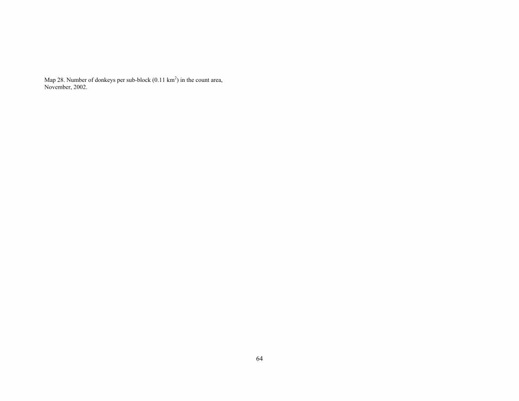
64

Map 28. Number of donkeys per sub-block (0.11 km2) in the count area, November, 2002.

65

Map 29. Number of domestic dogs per sub-block (0.11 km2) in the count area, November, 2002.

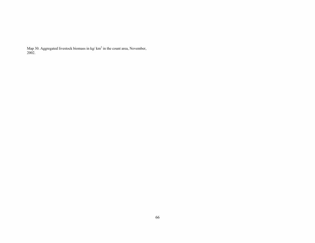
66

Map 30. Aggregated livestock biomass in kg/ km2 in the count area, November, 2002.

67

4.8 Wildlife and multiple species associations (MSA’s): how many and where? We counted individuals of 38 wildlife species in the 2002 count. There were 15 of these 38 species that we counted relatively well. We will present mostly the species we counted well; maps of the bat-eared fox, black rhino, bushbuck, crocodile, duiker, hare, honey badger, mongoose, leopard, tortoise are available on request. Do wildlife prefer the reserve (protected savanna) or the group ranches (pastoral savanna)? We compared wildlife density between the group ranches and the Mara reserve to find out where there were more wildlife (Tables 5 and 6). We found three different ways that wildlife responded to protection in the reserve and pastoralism in the group ranches:

1. No preference between protected and pastoral savanna: 6 species. Many species of wildlife were just as abundant in the reserve as in the group ranches. Many showed this same pattern in the count in 1999 and the one in 2002. These species included baboon, jackal, mongoose, waterbuck, wildebeest and zebra. Note that in absolute terms, there were many more wildebeest and zebra in the reserve than the group ranches, but they were clustered so strongly that there is no significant statistical difference in their average densities in the two areas.

2. Preference for pastoral savanna: 5 species. In both 1999 and 2002, there were more dik dik, giraffe, and impala in the group ranches than the reserve. Vervet monkeys showed some preference for the group ranches with more in 1999 but no difference in 2002. There were more Thomson’s gazelles on the group ranches in 2002 only.

3. Preference for protected savanna: 16 species. In both years, there were more crocodile, eland, elephant, hartebeest, hippo, hyena, lion, ostrich, reedbuck, tortoise and warthog in the reserve than in the group ranches. There were the same number of

buffalo, Grant’s gazelle, and oribi in the reserve and ranches in 1999, but more in 2002. Topi and vulture were more abundant in the reserve during the drought year of 1999, but showed no preferences in 2002.

We did not observe enough bat-eared foxes, bushbucks, cheetahs, duikers, hares, honey badgers, leopards, and rhinos to make distinctions between the reserve and group ranches for these species. These data strongly support the conclusion that most species of wildlife (3 times more species) prefer to forage in the reserve than in the group ranches. We must be cautious about what this means. When there are more wildlife in the reserve, are they repelled by conditions on the group ranches or attracted to conditions in the reserve (or both)? Why? Similarly, when there are more wildlife in the group ranches, are they attracted to the group ranches or driven out of the reserve or both? Why? As becomes clear later in this report, the answers to these questions are probably not simple.

4.9 How were types of wildlife and MSA’s distributed around the counting area? Wild herbivores. Wild herbivores (plant eaters) gathered in two distinct bands in the counting area in November 2002 (Map 31). One band was just north of the reserve boundary in south Koyiaki Group Ranch to the west of the Olare Orok River and to the east of the Ntiakitiak River. Another band was in the southern half of the reserve from the western edge of the Triangle across to Keekorok. There were very few wildlife near and south of Ol Doinyo Orinka, Aitong, in Talek, and in parts of Musiara and Sekanani. It is striking how areas with lots of wildlife were often surrounded by areas with very little wildlife, when mapped at the resolution of 1 km.

68

Wild carnivores. Wild carnivores (meat eaters) were not necessarily found with their prey (Map 32). For example, there were fewer carnivores with the southern band of herbivores in the reserve than there were within an area with comparatively few wildlife in central Musiara in the reserve. We saw no carnivores near Ol Doinyo Orinka, within Talek town or in Ol Chorro Oirowua. Carnivores did not concentrate in a particular place except for just north of the bomas along the Ntiakitiak River in the group ranch. Note that any conclusions about the abundances and distribution of carnivores are tentative because these species are very hard to count during a short, ground count. All wildlife species and multiple species associations. The greatest concentration of wildlife species was in the central Triangle, to the west of the Olare Orok in the group ranch, just east of the Ntiakitiak in the group ranch, Koyiaki Group Ranch, northeast of Talek in the Olkinyei area, and to the east of the Mara River in the reserve (Map 33). We saw few species in the rest of the Triangle, around the Ol Keju Gem, near Ol Doinyo Orinka and Aitong, in Ol Chorro Oirowua and near the base of the Bardamat Hills. Surprisingly, there were few species but lots of biomass south of the Ol Keju Gem, in the eastern Triangle and around Keekorok. Similarly there was little biomass, but many species just to the northwest of Talek. This means that during the count, many areas of the reserve were good places to find many animals and large-bodied animals, but the most diverse group were in the group ranch. A multiple species association (MSA) is two or more wildlife species in a group with individuals not more than 300 m from each other. They associate in MSA's for a variety of reasons:

1. To share vigilance (watching) costs against ambush killing predators (lions) and to reduce the individual risk of being killed by gathering in big groups.

2. To access areas where soils are particularly fertile and contain particularly high quality grass.

3. To graze on relatively short grass areas growing in soils that have been nutritionally enhanced by the presence of dung from abandoned Maasai boma sites.

4. To graze on relatively short grass that is repeatedly grazed and fertilized by wildlife droppings and thus kept in a younger, more nutritious growth state.

5. To associate at resting locations that are intermediate between access to water and access to forage of higher quality. Note: MSA's are most developed in the middle of the day after the morning grazing period and before the afternoon and evening grazing period.

6. Finally, wild species nearest in body size to domestic livestock (between 18 and 200 kg) may associate together to prevent pastoralists and their livestock from using these areas.

In the Mara during the 2002 count, only the largest MSA's in the group ranch and in the reserve have been preliminarily analyzed (Map 34). They cover 11% of the areas sampled on the ranch and the reserve. On the group ranches, there were fewer, larger MSA's and they were distributed in a broad 10 - 20 km band running parallel to the northern boundary of the reserve. The 17 largest MSA's averaged 6.5 km2 in size but ranged between 1.5 km2 and 23 km2. In the reserve, there were 32 MSA's ranging in size between 1.5 km2 and 15.3 km2. MSA's in the reserve were smaller than those on the group ranch. Their average size was 4.3 km2 and they were much more widely scattered. MSA's in both the group ranches and the reserve are strongly associated with relatively short grass areas averaging 6.5 cm leaf height or less. These short grass areas in turn are strongly associated with the following:

1. recent burns,

69

2. the grazing areas of cattle both on the group ranches and on the northern edge of the reserve where cattle penetrate up to 8 km into the reserve on a daily basis in the dry season,

3. in the reserve they are also associated with the very short grazing lawns that are maintained by hippos emerging at night to graze within 5 km of the Mara and Talek Rivers, and

4. in the group ranches, MSA's are strongly associated with the broad band of tsetse-infested woodland that parallels the reserve boundary on the rocky slopes between the lower and higher grassland plains of the Koyiaki Group Ranch.

In order to develop an effective conservation strategy for the Mara, it is important to try to understand the conditions which lead to MSA formation, expansion, contraction, and collapse. Very large herbivores which are nearly predator-proof are almost never found as members of MSA's, and when they are found in MSA's the association is not long lasting. Thus, cape buffalo (400 kg), elephant (1400 kg), hippo and rhino (each 1000 kg) occur least (in order) in MSA's. In contrast, for five resident herbivore species, MSA membership is most frequent. These are, in order of frequency of association, Thomson's gazelle (20 kg), topi (100 kg), Grant's gazelle (40 kg), impala (40 kg), and warthog (40 kg). For at least three of these species (topi, Grant’s and impala), MSA association is on average 70% more frequent on the group ranch than it is in the reserve. This suggests that avoidance of livestock and/or people may be a factor restricting wildlife movement in the group ranch areas. The principal migratory species, zebra and wildebeest, are typically found in MSA's when they are resting or grazing, but are often in single species grouping or mobile migratory paired MSA's when they are moving. In addition to these 7 most frequent members of MSA's, Maasai giraffe, a 750 kg browser, and Maasai ostrich (110 kg) are only occasionally found in MSA's.

Finally, again in order of least occurrence: eland (350 kg), Coke's hartebeest (140 kg) and waterbuck (160 kg) -- the latter are both territorial antelope that select for longer grass and compete poorly with cattle -- are usually not found in MSA's. It is striking that on about 50 to 60 % of the group ranch, where the distribution of bomas and livestock is most uniform (and dense), MSA formation no longer occurs. In both the group ranch and the reserve, lions, hyenas and cheetahs are typically found within a few kilometres of the outside edge of MSA's and probably contribute predator pressure for their formation. In order to be persistent after predator attacks, MSA's must have more than 300 members and more than 4 species. Understanding the development of MSA's that are small and cover less than a kilometre that will grow into to large MSA's of 10 km2 or more containing thousands of animals is an urgent task and will be part of the further analysis of this data set. If we can do this, we can better protect the classic savanna assemblage of many species living within sight of one another.

70

Map 31. Aggregated wild herbivore biomass in kg/ km2 in the count area, November, 2002.

71

Map 32. Aggregated wild carnivore biomass in kg/ km2 in the count area, November, 2002.

72

Map 33. Number of wildlife species per sub-block (0.11 km2) in the count area, November, 2002.

73

Map 34. Distribution of multiple species associations in the count area, November, 2002.

74

4.10 How were individual species distributed around the counting area? The order of species that follow is first by what they feed on and then by body weight from heaviest to lightest (with the exception of wildebeest and zebra which come first among the grazers because they are so abundant). Grazers (grass and leafy herb eaters). Wildebeest and zebra: abundant in the protected and pastoral savanna. Migrating wildebeest and zebra, mixed with fewer numbers of resident animals (Maps 35 and 36), made up much of the biomass in the wild herbivore concentration points (Map 31). We counted about 6 times as many wildebeest in the reserve as the group ranches in 1999 (13 vs 79/km2) and 5 times as many in 2002 (26 vs 108/km2). In the larger counting area in 2002, we counted 135,000 wildebeest in the reserve, with more than half of those in the Sekanani area alone. This is more than a quarter of all the animals we counted altogether. However, a statistical comparison of the average densities between the two areas shows no difference because there is so much variability in the abundance of this species from place to place. It is also not sensible to compare the number of wildebeest or zebra between the reserve and group ranches because most of the migrants happened to be in the southern part of the reserve on their return to the Serengeti, making a direct comparison invalid. We planned the count so that it would take place after the migration left the Mara for the Serengeti so that we would count only residents, but inadvertently caught the tail end of this huge group of animals in both 1999 and 2002. Similarly, our teams counted about 1.5 times as many zebra in the reserve than group ranches in 1999 and 1.3 times as many in 2002; but, again, the average densities are not different in a statistical sense. Our counting teams found very large groups of wildebeest and zebra in the southern reserve on both counts, presumably made up of Serengeti migrants. Wildebeest gathered in large groups in the central

Triangle, near Keekorok and west of the Olare Orok. Wildebeest appeared to be strongly attracted to recent burns and very short grass (see Map 11). Zebra clustered with the wildebeest here, but also in the southeastern Triangle and east of the Ntiakitiak. Zebra clustered with wildebeest on burns but also where there was no evidence of recent burns and grass was of medium height. Hippo: strong preference for protected waters. There were 4-6 times as many hippos in the rivers of the reserve (0.4 to 0.6/km2) than in the group ranches (0.1 to 0.09/km2) in both years (Table 5). Most of the hippos lived in the Mara River, with many more hippos in the part of the Mara that passes through the reserve than the part that crosses the group ranches (Map 37). Our teams counted hippos along the length of the Talek, in pools on the Ntiakitiak and Ol Keju Gem, but not in the Olare Orok River. No hippos were counted in the Talek River near Talek village. Cape buffalo: strong preference for protected savanna. Buffalo were 2.5 times more common in the reserve than group ranches in 1999 and 16 times more common in 2002 (Table 5). We counted 84% fewer buffalo in the group ranches in 2002 than 1999. In 2002, buffalo gathered in the tall grass areas south of the Ol Keju Gem and in the northern Triangle (Map 38). We also counted many buffalo along the Mara, Talek and Ol Keju Gem Rivers. Buffalo compete strongly with cattle for forage, thus it is no surprise that they prefer to graze in the southern reserve where no livestock graze. Defassa waterbuck: no preference for protected or pastoral savanna. Waterbuck were equally abundant in the reserve as the group ranches. Waterbuck were concentrated along permanently flowing rivers, especially in Mara and Talek Rivers (Map 39). Waterbuck also inhabited several areas with tall grass, like the northern Triangle. There were many

75

waterbuck in the northern Mara, in the savannas between Aitong and the Mara River. Coke’s hartebeest: strong preference for protected savanna. Coke’s hartebeest was rare in the reserve (0.38/km2) and the group ranches (0.14/km2) in 1999 with similar abundances in 2002. This is a species that clearly prefers the protected area more than the pastoral area, perhaps because they often compete with cattle for forage (Kingdon 1997). Groups of hartebeest were most common on the drier eastern part of the reserve in Sekanani than in the Triangle or Musiara (Appendix Table A4, Map 40). We found no hartebeest on the private ranch, Ol Chorro Oirowua. Maasai ostrich: strong preference for protected savanna. Ostrich were 6 times more abundant in the reserve than group ranches in 1999 (0.17 vs. 0.03/km2, Table 5) and 3 times more abundant in 2002 (0.30 vs. 0.09/km2). Ostrich were spread fairly evenly throughout the reserve, with fewer in the wetter Triangle (Map 41). Group sizes appeared to be larger in the group ranches than the reserve. Topi: weak preference for protected savanna. There were more than 1.6 times as many topi (Map 42) in the reserve (4.4/km2) as the group ranches (2.7/km2) in 1999, but there were only 1.1 times as many in 2002 (4.2 compared with 3.8/km2, no significant difference). Topis avoided areas with very long grass, similar to Thomson’s. They also preferred areas with shrub cover. We found the largest concentration just east of the Ntiakitiak with Thomson’s gazelles in recently burned areas. Warthog: strong preference for protected savanna. There were almost twice as many warthogs in the reserve than group ranches in both years (Table 5). Most of the warthogs in the reserve were in the Musiara area

and the northern Triangle (Map 43). Warthogs seem to avoid the high grass areas south of the Ol Keju Gem River. Bohor reedbuck: strong avoidance of pastoral savanna. We found no reedbuck in the group ranches either year. There were 170 reedbuck seen by our teams in the reserve (Map 44). Reedbuck were evenly spread throughout the reserve with some concentration around the Musiara swamps. Thomson’s gazelle: weak preference for pastoral savanna. Thomson’s gazelles (Map 45) were the third most abundant species of wildlife in our Mara count, which included many migrants and some residents. We counted about 23,000 Thomson’s gazelles in 1999 and about 35,000 in 2002 within the same counting area. This species was equally distributed between the group ranches and reserve in 1999, but were more common on the group ranches than reserve in 2002. These gazelles often clustered with wildebeest and topi, especially on recently burned areas in the Triangle and just east of the Ntiakitiak River. They were also common just south of Talek village along the Talek River, in an area that had not burnt recently. Thomsons’ gazelles avoided the long grass areas south of the Ol Keju Gem River, in the northern Triangle and in the north in Ol Chorro Oirowua. We expect this species to be more attracted to short grass than any other species because of their nutritional requirements and their small size makes detection of predators difficult when grass grows to moderate heights. Tortoise: weak preference for protected savanna. We found only 1 tortoise in the count areas in 1999, but 39 in 2002. We saw 3 times as many tortoises in the reserve as group ranches in 2002. Note that our count of tortoises will strongly under-estimate the real population size and distribution patterns because they are so hard to see in tall grass. We saw most of the tortoises close to rivers and in groups of one (Map 46).

76

Mixed feeders (grass, shrub and tree eaters). African elephant: strong preference for protected savanna. We found 6-7 times more elephants in the reserve than the group ranches (Table 5). There were also larger herds in the reserve than group ranches (Map 47). Most of the elephants were in the southern part of the reserve, away from the areas where cattle graze within the northern border of the reserve. We found many elephants, as expected, along water courses, particularly the Ol Keju Gem River in the reserve. Cape eland: strong preference for protected savanna. We counted 5 times as many eland in the reserve than group ranches in 1999 and 9 times as many in the reserve in 2002. Like elephant, the eland clustered in the southern part of the reserve, away from pastoralists and their livestock (Map 48). Eland seemed to gather in areas of different grass heights. Grant’s gazelle: Weak preference for protected savanna. There were the same number of Grant’s in the group ranches and reserve in 1999, but 35% more in the reserve in 2002. Grant’s, in contrast to eland, clustered around the reserve-ranch boundary, and avoided the southern reserve (Map 49). There were few Grant’s in the Triangle, with the most in the Musiara section. There were also few Grant’s in Ol Chorro Oirowua. Impala: Strong preference for pastoral savanna Impala were the fourth most abundant wildlife species we counted, after wildebeest, zebra, and Thomson’s gazelle. Impala clustered along the Mara and Talek rivers in the reserve, the only places where woody plants are common in the reserve (Map 50). Most of the impala were just north of the reserve boundary, especially north of Talek in the wooded savanna there. They also clustered in the Croton patches near the reserve and in the Acacia gerrardii woodland where we found many tsetse flies. Impala may prefer the group ranches because their dietary overlap with livestock is low to

moderate, depending on the season, and woody plants are more common on the ranch than in the reserve. Bushbuck: No preference – sample sizes too low? We found only 22 bushbuck in the two counts together. This species is very hard to find and we strongly under-counted its population. The few that we found were mostly along rivers and mostly in the reserve (Map 51). Duiker, oribi and hares: Too few of these species were counted to make reliable comparisons between the reserve and group ranches. Nearly all the duikers we counted were in the high grass areas south of the Ol Keju Gem in the reserve (Map 52). We found almost all the oribi in the wetter Triangle (Map 53). Hares were equally abundant in the reserve and group ranches and were found mostly in western Koyiaki in the most wooded part of the count area (Map 54). Browsers (mostly tree and shrub eaters). Giraffe: strong preference for pastoral savanna. There were more than twice as many giraffe in the group ranches than in the reserve in both years. We found many of the giraffe in the tsetse-infested belt of Acacia woodlands about 7-10 kms north of the reserve (Map 55). The giraffe in the reserve clustered along the riverine areas, the only places with significant numbers of trees. Black rhino: strong preference for protected savanna. We counted 11 rhinos in the entire count area in 2002. One rhino was in the rhino sanctuary near Ol Chorro Oirowua and the other ten were close to each other south of the Ol Keju Gem in the high grass within the reserve (Map 56). Dik dik: strong preference for pastoral savanna. We counted 5 times as many dik dik in the group ranches than the reserve in 1999 and 10 times as

77

many in 2002. Most of the dik dik clustered in the woody eastern part of Koyiaki and near Ol Doinyo Orinka (Map 57). Carnivores and scavengers (meat and carrion eaters). We did not count any of the carnivores well. For some species, this was because of their behaviour, others were small, another in water, another flying. We present the data here, urging the reader to take caution in interpreting this information. Lion: strong preference for protected savanna. We counted 100 more lion in the same count area in 2002 than 1999. We counted 9 times as many lions in the reserve than group ranches in 1999 but only 2.5 times more in 2002. There were several large groups in both the reserve and group ranches, but only smaller groups in the Triangle (Map 58). The big concentrations of lions were south of the Ol Keju Gem with the migration and around the Talek River near Intrepids Lodge. Crocodile: strong preference for the protected savanna. We counted 10-15 times as many crocodiles in the reserve as the group ranches. Like hippos, most crocodiles were in the Mara River, but unlike hippos, we did not find any crocodiles in the Talek River (Map 59). Leopard and cheetah: too few counted. We counted 2 leopards in 1999 and 1 leopard in 2002, all in the reserve (Map 60). Our teams saw 11 cheetah equally distributed between the reserve and group ranches in 1999. In 2002 in the same area, we counted 15 cheetah, with 27% in the group ranches and 73% in the reserve. Our few observations of cheetah were spread throughout the count area (Map 61). We cannot make any conclusions about the populations of these species. Hyena: strong preference for the protected savanna. We found about twice as many hyena in the reserve as the group ranches in both years. Despite

the greater number of hyena in the reserve, there were large numbers in the group ranch, especially in the Ntiakitiak River area. To give an idea of how well we counted hyena, we counted 2 hyena in the same area around Talek where the hyena research team from Michigan State know there is a clan of 50 hyena. Recent work by this research team shows that hyena behaviour is strongly affected by the presence of people and livestock21 (Map 62). Jackal: no preference. Our teams counted about the same density of jackals in the group ranches and reserve in both years. Jackals were everywhere, probably the most evenly distributed species that we counted (Map 63). Honey badger, bat-eared fox, honey badger: too few counted. Honey badgers were rare. Our teams found only 1 in 1999 and 25 in 2002. Of the 25, 1 was in the group ranch and 24 in the reserve (Map 64). We counted 18-20 bat-eared foxes each year, but too few to come to specific conclusions about their distribution. Bat-eared foxes seemed to avoid high grass areas and areas with no trees (Map 65). Vultures: Weak preference for protected savanna. Most of the vultures we counted were on the ground, feeding on wildlife kills. We did not attempt to make a thorough count of vultures flying high in the sky. Vultures preferred to be where the majority of the carcasses were: in the reserve. Most of them were in the southern reserve with the wildebeest migration (Map 66). Mongoose: no preference. There were the same number of mongoose in the reserve and group ranches in 1999 and there appeared to be 40% more mongeese in the reserve than group ranch in 2002 (although this difference

21 Boydston and others 2003

78

was not significant). This species was also very evenly distributed across the count area (Map 67). Primates. Baboon: no preference. We counted about the same density of baboons in the reserve as the group ranches. Baboon group sizes appeared to be larger in the group ranches than in the reserve (Map 68). Vervet: weak preference for pastoral savanna. In 1999, there were 15 times more vervets on the group ranch than the reserve, but no difference in 2002. Vervets were spread across the count area, and, like baboons, seemed to cluster in larger groups in the group ranches (Map 69). 4.11 Private compared with communal ranching A comparison of the density of wildlife and livestock in Ol Chorro Oirowua with those in the group ranches may give some comparison of private compared with communal management of livestock and wildlife. However, because Ol Chorro ranch is relatively small and far from the Mara reserve, we would expect fewer wildlife species here and perhaps fewer numbers of each type of wildlife that are present. There were fewer livestock on Ol Chorro than the group ranches (see Appendix Table A4). There were also many species missing from the half of Ol Chorro that we counted compared with the much larger group ranches, but we expected many to be missing. The species missing in Ol Chorro but found on the other ranches included: bat-eared fox, buffalo, duiker, hartebeest, hyena, jackal, lion, tortoise, vervet, and vulture. However, Ol Chorro is home to the only rhino we found outside the reserve. In general, when a wildlife species was present, there were many fewer on Ol Chorro than the other group ranches. This last point is significant, and may point to differences in management on Ol Chorro compared to the group ranches, or to differences in the suitability of the habitat for wildlife in these two areas.

4.12 Transmara (Triangle) compared with Narok part of the reserve There was no appreciable difference in the abundance of wildlife comparing between the Transmara (Triangle) and Narok (Musiara and Sekanani together) parts of the reserve (Table A4 in Appendix). We found about 30% more carnivores in the Narok part of the reserve than in the Transmara. This was the case in spite of the fact that there were about twice as many livestock in the Narok part of the reserve as in the Transmara part. By species, there were many more species that were more abundant in the Narok side of the reserve than the Transmara. Five species were more abundant in the Transmara than the Narok part of the reserve (bushbuck with 79% more in the Transmara, oribi with 79% more, bat-eared fox with 61% more, buffalo with 60% more, and waterbuck with 56% more). There were 12 species more abundant in the Narok than Transmara part of the reserve (ostrich with 86% more in the Narok part of the reserve, Grant’s gazelle with 85% more, lion with 81% more, cheetah with 66% more, eland with 63% more, duiker with 62% more, hyena with 62% more, baboon with 56% more, jackal with 52% more, hartebeest with 52% more, topi with 37% more, vervet monkey with 32% more). In general, the species that are more water dependent (waterbuck) or that can tolerate coarse grass (buffalo) were more abundant in the Transmara than in the Narok part of the reserve, probably because the Transmara is wetter than the Narok side. There was no appreciable difference in the abundance of dik-dik, zebra, giraffe, elephant, Thomson’s gazelle, wildebeest, reedbuck, impala, vultures, warthog and mongoose between Narok and Transmara parts of the reserve. There were no rhinos, honey badgers, leopards, hares or crocodiles counted in the Transmara, but for all species but rhino, this was caused by the way we attributed animals (all crocodiles and hippos in the Mara River were counted as ‘in’ the Narok part of the reserve in our analysis so far, which is not correct) or our ability to detect the species (for example, tortoise, hare, leopard).

79

Map 35. Number of wildebeest per sub-block (0.11 km2) in the count area, November, 2002.

80

Map 36. Number of Burchell’s zebra per sub-block (0.11 km2) in the count area, November, 2002.

81

Map 37. Number of hippo per sub-block (0.11 km2) in the count area, November, 2002.

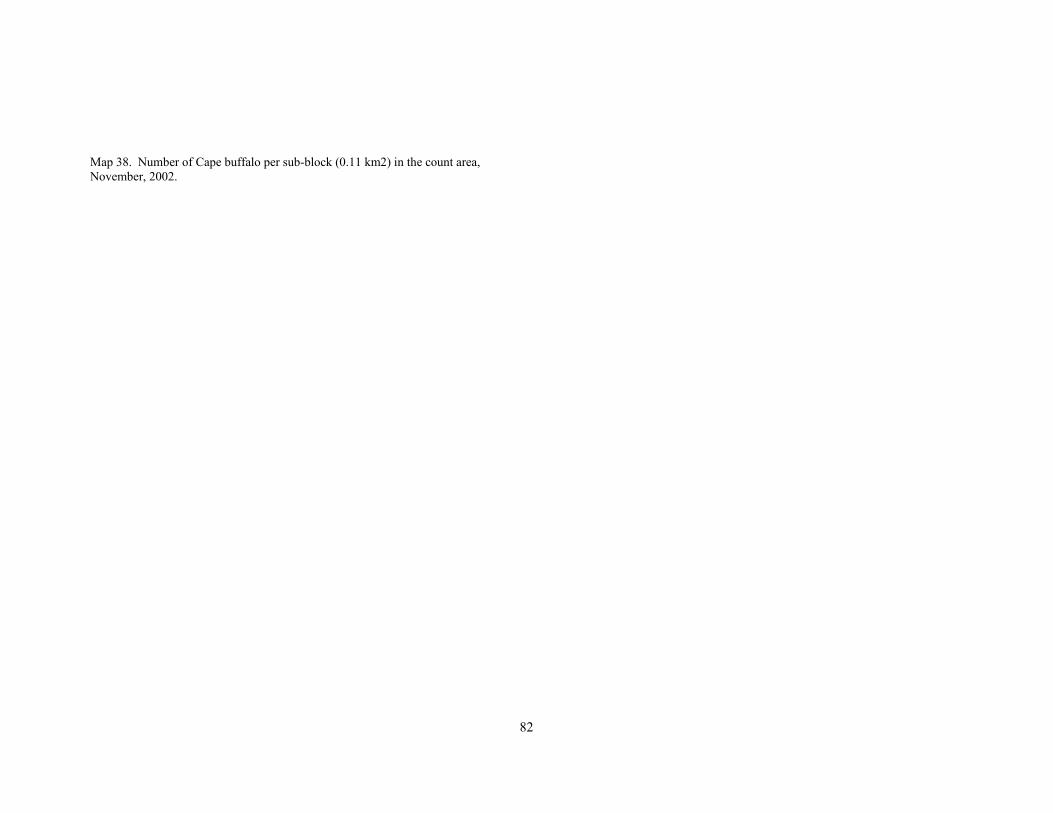
82

Map 38. Number of Cape buffalo per sub-block (0.11 km2) in the count area, November, 2002.

83

Map 39. Number of Defassa waterbuck per sub-block (0.11 km2) in the count area, November, 2002.

84

Map 40. Number of Coke’s hartebeest per sub-block (0.11 km2) in the count area, November, 2002.

85

Map 41. Number of Maasai ostrich sub-block (0.11 km2) in the count area, November, 2002.

86

Map 42. Number of topi per sub-block (0.11 km2) in the count area, November, 2002.

87

Map 43. Number of warthog per sub-block (0.11 km2) in the count area, November, 2002.

88

Map 44. Number of Bohor reedbuck per sub-block (0.11 km2) in the count area, November, 2002.

89

Map 45. Number of Thomson's gazelle per sub-block (0.11 km2) in the count area, November, 2002.

90

Map 46. Number of tortoise per sub-block (0.11 km2) in the counting area, November, 2002.

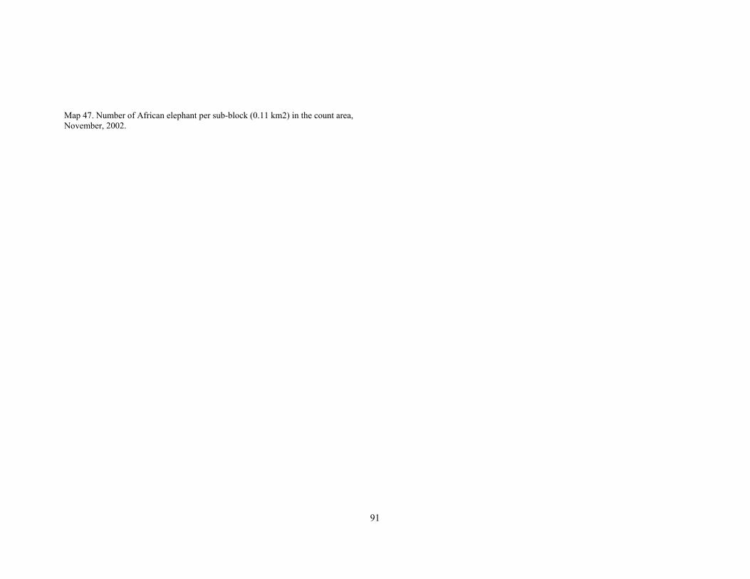
91

Map 47. Number of African elephant per sub-block (0.11 km2) in the count area, November, 2002.

92

Map 48. Number of Cape eland per sub-block (0.11 km2) in the count area, November, 2002.

93

Map 49. Number of Grant’s gazelle per sub-block (0.11 km2) in the count area, November, 2002.

94

Map 50. Number of impala per sub-block (0.11 km2) in the count area, November, 2002.

95

Map 51. Number of Eastern bushbuck per sub-block (0.11 km2) in the count area, November, 2002.

96

Map 52. Number of duiker (all species)per sub-block (0.11 km2) in the count area, November, 2002.

97

Map 53. Number of oribi per sub-block (0.11 km2) in the count area, November, 2002.

98

Map 54. Number of hare (all species) per sub-block (0.11 km2) in the count area, November, 2002.

99

Map 55. Number of Maasai giraffe per sub-block (0.11 km2) in the count area, November, 2002.

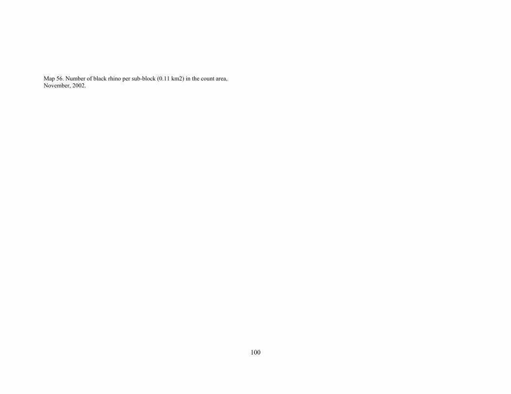
100

Map 56. Number of black rhino per sub-block (0.11 km2) in the count area, November, 2002.

101

Map 57. Number of Kirk’s dik-dik per sub-block (0.11 km2) in the count area, November, 2002.

102

Map 58. Number of lion per sub-block (0.11 km2) in the count area, November, 2002.

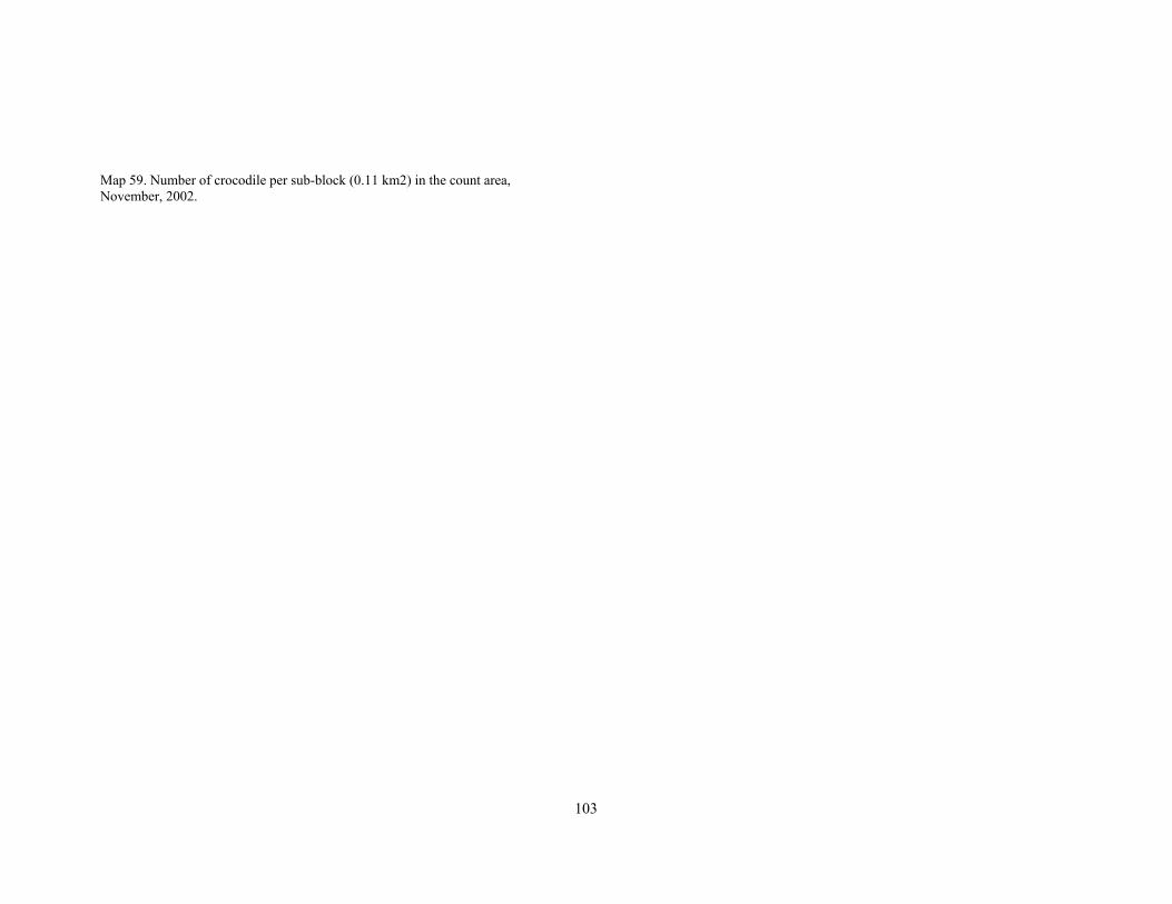
103

Map 59. Number of crocodile per sub-block (0.11 km2) in the count area, November, 2002.

104

Map 60. Number of leopard per sub-block (0.11 km2) in the count area, November, 2002.

105

Map 61. Number of cheetah per sub-block (0.11 km2) in the count area, November, 2002.

106

Map 62. Number of spotted hyena per sub-block (0.11 km2) in the count area, November, 2002.

107

Map 63. Number of jackal species per sub-block (0.11 km2) in the count area,November, 2002.

108

Map 64. Number of honey badger per sub-block (0.11 km2) in the count area, November, 2002.

109

Map 65. Number of bat-eared fox per sub-block (0.11 km2) in the count area, November, 2002.

110

Map 66. Number of vulture (all species) per sub-block (0.11 km2) in the count area, November, 2002.

111

Map 67. Number of mongoose (all species) per sub-block (0.11 km2) in the count area, November, 2002.

112

Map 68. Number of Anubis baboon per sub-block (0.11 km2) in the count area, November, 2002.

113

Map 69. Number of vervet monkey per sub-block (0.11 km2) in the count area, November, 2002.

114

4.13 Did wildlife numbers change between 1999 and 2002?

To compare wildlife numbers between the two years, we used only the 2002 counts that overlapped with the smaller area counted in 1999 (Tables 5 and 6). We found six different ways that wildlife densities changed between 1999 and 2002:

1. More in 1999, but only in the reserve: 1 species, possible conflict over water in the drier year of 1999. We found that elephant was the only species to occur at a higher density in the reserve in 1999 compared to 2002.

2. More in 2002 in both group ranches and reserve: 12 species = population growth and in-migration after drought. Grant’s gazelle, hare, hyena, impala, jackal, mongoose, Thomson’s gazelle, tortoise, warthog, wildebeest, and zebra

3. More in 2002 only in the reserve but not the ranches: 5 species = population increase after drought, but only in the reserve. Baboon, buffalo, eland, lion, reedbuck and vultures.

4. More in 2002 only in the ranches and not the reserve: 2 species= little habitat available in the reserve. Dik dik and giraffe

5. More in 1999 in the reserve, more in 2002 in the ranches: 2 species = retreat to reserve during dry year, prefer group ranch in wetter year. Topi and waterbuck

6. No difference in both years: 5 species. Crocodile, hartebeest, hippo, ostrich, vervet monkey.

We did not observe enough bat-eared foxes, bushbucks, cheetahs, duikers, honey badgers, leopards, oribi, and rhinos to make distinctions between the reserve and group ranches for these species. Why these patterns? Why were there so many more wildlife and livestock in both the group ranches and reserve in 2002 than in 1999? First, as

mentioned under the vegetation section above, we estimate that there was about double the green grass biomass in the 2002 than in 1999 in both the reserve and group ranches. The difference between the reserve and group ranches (more green grass in the reserve) was more pronounced in 1999 than 2002. This alone could explain the increased populations of livestock and wildlife in 2002 than 1999. It is difficult to come to this conclusion from rainfall records alone (Figure 3), because wet season rainfall in 1999 was lower than 2002 but dry season rainfall was higher22. The low numbers in 1999 probably reflect a combination of movement out of the system in search of better water and forage, and drought related mortality. Similarly, intrinsic population increase combined with in migration into the system in the moderate year of 2002 may account for observed increases between 1999 and 2002. Our carcass data (below) seems to support this interpretation – there were many more carcasses in 1999 than 2002 – although there are other explanations for this. 4.14 Carcasses We found 10-12 times as many fresh carcasses (by density) in the reserve than in the ranches in 1999 and 2002Table 7). Wildebeest contributed 75% (1999) and 86% (2002) of all carcasses counted in the reserve and 42% of all carcasses seen on the group ranches in both years. Zebra carcasses were the second most common type of carcasses recorded for the reserve (both years) and the most common on the group ranches in 1999. In 2002, impala carcasses were the second most common type we found in the group ranches. As we mentioned above, this is probably a result of drought mortality. We did not find any livestock carcasses in either year. We found most of the carcasses in the southern reserve with the wildebeest migration, as we expected (Map 70). There were twice as many wildebeest and zebra per lion in the reserve in 1999 (1713) than 2002 (941) even though there were 30% fewer wildebeest and and 50% fewer 22 Research in the Serengeti (Mduma and others 1999) shows that dry season rainfall is particularly important to the populations of many of the grazers.

115

zebra in the reserve in 1999 than 2002. Lion populations were only 65% lower in the reserve in 1999 than 2002. This may suggest that the few lion were more successful hunters in 1999 than 2002 (weaker prey due to drought?) or that there was significant drought-related mortality (independent of lion kills) in 1999 than 2002. However, these calculations need to be treated with caution because our lion and hyena counts under-estimate the number of these predators present.

116

Map 70. Number of fresh carcasses per sub-block (0.11 km2) in the count area, November, 2002.

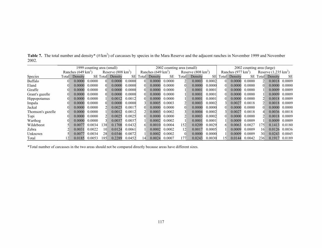
117

Table 7. The total number and density* (#/km2) of carcasses by species in the Mara Reserve and the adjacent ranches in November 1999 and November 2002.

1999 counting area (small) 2002 counting area (small) 2002 counting area (large) Ranches (649 km2) Reserve (808 km2) Ranches (649 km2) Reserve (808 km2) Ranches (977 km2) Reserve (1,235 km2) Species Total Density SE Total Density SE Total Density SE Total Density SE Total Density SE Total Density SEBuffalo 0 0.0000 0.0000 0 0.0000 0.0000 0 0.0000 0.0000 2 0.0003 0.0002 0 0.0000 0.0000 2 0.0018 0.0009Eland 0 0.0000 0.0000 0 0.0000 0.0000 0 0.0000 0.0000 0 0.0000 0.0000 0 0.0000 0.0000 0 0.0000 0.0000Giraffe 0 0.0000 0.0000 0 0.0000 0.0000 0 0.0000 0.0000 1 0.0001 0.0001 0 0.0000 0.0000 1 0.0009 0.0009Grant's gazelle 0 0.0000 0.0000 0 0.0000 0.0000 0 0.0000 0.0000 1 0.0001 0.0001 0 0.0000 0.0000 1 0.0009 0.0009Hippopotamus 0 0.0000 0.0000 1 0.0012 0.0012 0 0.0000 0.0000 1 0.0001 0.0001 0 0.0000 0.0000 2 0.0018 0.0009Impala 0 0.0000 0.0000 0 0.0000 0.0000 3 0.0005 0.0003 2 0.0003 0.0002 3 0.0027 0.0018 2 0.0018 0.0009Jackal 0 0.0000 0.0000 2 0.0025 0.0017 0 0.0000 0.0000 0 0.0000 0.0000 0 0.0000 0.0000 0 0.0000 0.0000Thomson's gazelle 0 0.0000 0.0000 1 0.0012 0.0012 2 0.0003 0.0002 3 0.0004 0.0002 3 0.0027 0.0018 4 0.0036 0.0018Topi 0 0.0000 0.0000 2 0.0025 0.0025 0 0.0000 0.0000 2 0.0003 0.0002 0 0.0000 0.0000 2 0.0018 0.0009Warthog 0 0.0000 0.0000 3 0.0037 0.0037 1 0.0002 0.0002 1 0.0001 0.0001 1 0.0009 0.0009 1 0.0009 0.0009Wildebeest 5 0.0077 0.0034 138 0.1708 0.0432 6 0.0010 0.0004 152 0.0209 0.0029 6 0.0063 0.0027 175 0.1413 0.0180Zebra 2 0.0031 0.0022 10 0.0124 0.0061 1 0.0002 0.0002 12 0.0017 0.0005 1 0.0009 0.0009 16 0.0126 0.0036Unknown 5 0.0077 0.0034 28 0.0346 0.0072 1 0.0002 0.0002 0 0.0000 0.0000 1 0.0009 0.0009 30 0.0243 0.0045Total 12 0.0185 0.0053 185 0.2289 0.0452 14 0.0024 0.0007 177 0.0243 0.0030 15 0.0144 0.0042 236 0.1917 0.0189 *Total number of carcasses in the two areas should not be compared directly because areas have different sizes.

118

4.15 How are wildlife distributed around water in the reserve and group ranches?

We analysed all the wildlife and livestock maps to discover any effects of protection and pastoralism on where animals distribute themselves on the landscape. We created a map of distance to water (Map 71) to complete this analysis. Comparing rivers and water points between the reserve and group ranches. The reserve and group ranches had strikingly similar drainage characteristics. About one quarter (26-30%) of all the sub-blocks we sampled contained a stream (small river) in the reserve (29.9%) and group ranches (26.2%). Only 9-10% of the sub-blocks contained a major river in either area. About 1% of the area of each sub-block was covered by a stream and only 0.3-0.4% covered by a major river. However, water points were more than twice as prevalent in the reserve as in the ranches with 7.4% of the 11,117 sub-blocks in the reserve and only 3.5% of the 8,794 sub-blocks in the group ranches containing water. Many of the differences may be in abundance of seasonal pools in the reserve. How were livestock and wildlife distributed around water? We developed a distance to water source map from the aerial count of water sources (Map 71). We used this map to try to understand how wildlife, livestock and vegetation are distributed around water, and then how protection and pastoralism affects those distributions (Figures 5a and 5b). All the herbivore species showed strong but contrasting distribution patterns around water as follows:

1. Clustering neither near nor far from water = humped distribution: For example, buffalo, eland, impala, ostrich, T. gazelle, topi, warthog, waterbuck, wildebeest and zebra were most common about 1-3 km from water in the reserve and group ranches in 1999. This distribution probably indicates that forage is

scarce near water23 due to heavy and constant grazing and trampling by animals visiting water sources and that the riparian woodland habitat fringing most water-courses in the Mara Area is unsuitable for most herbivores because of high predation risks near water24. It also suggests that wildlife cannot afford to forage too far from water because of the energy costs of walking long distances. However, forage is likely to be more abundant farther from water where the amount of grazing is lower. Thus, these species are balancing their need for water (near to water) and forage (far from water) by clustering neither near nor far from water. Another contributing factor to wildlife clustering at 1-3 km from water is that hippos grazing at night keeps the grass short within a few km of major rivers and this may attract grazers to the more nutritious grass where short grass makes it difficult for predators to hide.

2. Clustering close to water: Some species, like giraffe (reserve 1999, group ranches 2002), sheep and goats in both years, buffalo and impala in the reserve in 2002, waterbuck (2002 only) prefer to graze close to water. Buffalo and giraffe are usually too large to be attacked by predators (although these species are taken by predators) and thus grazing in bushy areas near water is not a great danger for them. Giraffe will also find their preferred forage more abundant near rivers, especially in the reserve.

3. Clustering far from water: We found several species far from water – giraffe (group ranches 1999, reserve 2002), G. gazelle (group ranches 1999), hartebeest (reserve in both years), ostrich (group ranches 2002) and cattle (group ranches in both years). Some of these species either need to access abundant forage far from water (cattle) or do not need to drink every day (hartebeest;

23 Western 1975, Herlocker 1992 24 Schaller 1972, Packer 1986

119

Kingdon 1997). We find the weak clustering of giraffe away from water in 2002 difficult to interpret.

4. Clustering both close and far from water = U-shaped distribution. We found species like buffalo and waterbuck (in 2002), elephant (1999 and 2002) and much of the livestock clustered both near and far from water, particularly in the reserve. For livestock, this means that our count caught herds while pastoralist brought them to drink and also while grazing far from water. For wildlife, these species need to take in large quantities of food each day and our count caught them both near water and in high grass areas far from water.

The cover and height of grasses, shrubs and trees was greater near water sources than far away in both 1999 and 2002 (figures available on request). Tree cover was most affected by water, with much higher cover around water sources than in the open plains, as is obvious from observation in the field. Bomas were clustered near water also (Figure 4). In both 1999 and 2002, most bomas were within about 2km from water. How does protection and pastoralism affect the distribution of wildlife around water? There are three ways that pastoralism and protection appear to affect how wildlife distribute themselves around water:

1. No effect: some species have the same distribution around water in the reserve and group ranches. This was rare. Only cattle and impala in 1999, elephant and waterbuck in 2002, donkeys, warthog, sheep and goats in both years had similar distributions from water in both the reserve and group ranches. This implies that pastoralism had little effect on the use of water by these species.

2. Pastoralism appears to push wildlife away from water: We found a ‘hump’ in the distribution of species like Thomson’s gazelle, impala, wildebeest (1999 only), elephant and ostrich (2002 only) farther away from water in the group ranches than in the reserve. This implies that livestock are competing with these species for water (and forage near water), so the wildlife stay farther from water when livestock are present. Stuart Williams25 found this to be true for Grevy’s zebra in Samburu in northern Kenya – Grevy’s stayed away from water in the day and usually came to drink at night when livestock were not at the water points. Note that if pastoralism is pushing wildlife away while livestock are using water points during the day, this increases predation risk greatly, since predators most often hunt and kill at night26, just when the water points are available for wildlife.

3. Pastoralism appears to attract wildlife to water points: The ‘hump’ in the distribution of eland, topi, Grant’s (2002 only), zebra (2002 only) and wildebeest (2002 only) was closer to water points in the group ranches than the reserve. Our predator counts seem to indicate that there are fewer predators in the group ranches than reserve (or that predators hide more on the group ranches than the reserve). Wild grazers may cluster closer to water points in the group ranches because they feel ‘safer’ there, either because predators are scarce or predators avoid people, as they appear to do around bomas (see below).

These strong differences in the distribution of animals around water may also indicate different ways that wildlife avoid competition with each other around water. For example, Thomson’s gazelle were most abundant in the group ranches in 2002 when the migratory eland, wildebeest and zebra populations were more abundant in the reserve. The changes in 25 Williams 1998 26 Kruuk 1972, Schaller 1972, Hanby et al. 1995

120

distributions of animals in different years is probably caused by changes in the amount of water and forage available in these two different years. Also, grazers may forage farther from water sources when there is less available to eat, but it is unclear from our data if the quantity of forage differed between 1999 and 2002. It does appear that many species grazed farther from water in 2002 than 1999, but this may also be a short-term effect of the onset of rain 1 day before our count started in 2002 and the lack of rain during the count in 1999. Similar patterns of distributions of species in relation to water were found in Amboseli, but the predominant effect was a displacement of wildlife from waterpoints, caused by human use.27

27 Worden and others 2003

Figure 4. Distribution of bomas from the nearest water sources in 1999 and 2002.

Distance from water in km

Num

ber o

f bom

as

0

20

40

60

80

100

120

140

0 1 2 3 4 5 6 7 8

1999 2002

121

Map 71. Distance to the nearest water source (in kilometres) in the count area, November, 2002.

122

Figure 5. Distribution of wildlife and livestock species around water in the reserve and group ranches in November 1999 and 2002.

123

124

4.16 How are wildlife distributed around bomas in the reserve and group ranches? We then created a map of the distance to the nearest boma, using the boma map we developed during the count (Map 72). We then asked how wildlife, livestock and vegetation are distributed around bomas in the reserve and group ranches. Grass cover and height were somewhat lower near bomas than far away, but the patterns were not strong. This weak pattern may be caused by the inter-mixing next to bomas of heavily grazed areas and little grazed areas saved by pastoralists for grazing reserves. Trees and shrubs were more abundant and taller close to bomas than far away, but these patterns were also weak. We found that wildlife distributed themselves around bomas differently in the reserve than group ranches (Figure 6a and 6b). Note that the effect of bomas outside but on the edge of the reserve probably spills over into the adjacent reserve, partly because many cattle graze in the reserve from bomas that are next to the reserve boundary. In the group ranches, nearly all the wildlife were neither near or far (= hump in the curve) from bomas. Ostrich, hartebeest, Grant’s gazelle, and waterbuck avoided bomas in 1999 but were collected at intermediate distances from bomas in 2002. The rest of the herbivores grazed at intermediate distance from bomas in both years. Bomas also appeared to have less influence on elephant distribution in the reserve in 2002. In the reserve, all wildlife grazed farther from bomas than they did in the group ranches. We think the animals in the reserve show a more accurate picture of the impact of bomas, because wildlife in the reserve can choose to graze very far from bomas in the southern reserve (or Serengeti). Animals on the group ranches have fewer choices: the farthest an animal

can go from a boma in the group ranch is 6 km, a distance well within the reach of grazing cattle within a day. Thus, wildlife on the group ranch can never ‘get away’ from livestock unless they graze in the areas heavily infested with tsetse, which are far from bomas. This implies that wildlife distributions are compressed in the group ranches by human use. Note that some of the patterns on these graphs are confused by the large number of migrating animals that happened to be in the southern reserve during our count, thus the patterns shown by wildebeest, zebra and Thomson gazelle should be treated with caution. In the reserve alone, wildlife chose to graze around bomas as follows:

1. Preference for grazing near bomas in 1999 and 2002: 2 species. Giraffe and impala

2. Preference for grazing far from bomas (9-15 km) in 1999, but near bomas in 2002: 5 species. Topi, Thomson’s gazelle, buffalo, waterbuck and elephant

3. Preference for grazing at intermediate distances from bomas (5-8 km): 1 species. Grant’s gazelle.

4. Preference for grazing far from bomas, both years: 6 species. Ostrich, zebra, hartebeest, warthog, eland and elephant only in 1999.

The patterns of wildlife around bomas in the group ranches and reserve surprised us. We expected to see wildlife avoiding bomas because livestock can compete with grazing wildlife for forage and dogs can attack or scare wildlife near bomas. Indeed, there appear to be several species that do prefer to graze far from bomas, probably for these reasons. These are species that may need protected savannas for survival However, there were several species of wildlife that preferred to graze neither close to nor far from bomas. We think there are at least four

125

explanations for this. First, livestock grazing may create expanses of nutrient- and energy-rich forage just beyond the heavily grazed areas surrounding bomas (or settlements). A second explanation is that wildlife may be attracted to the highly productive vegetation growing in nutrient-rich soils in abandoned bomas adjacent to inhabited bomas. In other ecosystems, wildlife and livestock preferentially graze on abandoned bomas compared with nearby areas with no settlements28. The third explanation is that wildlife, particularly smaller species highly susceptible to predation, may gather around settlements to avoid predators in the short grass grazed by livestock. A fourth reason that some species of wildlife congregate near people is that pastoralists may choose to settle in habitat near water and woody resources that is ideal for wildlife. Our data are most consistent with the forage nutrient and predation explanations, but only further research will give us confidence in the answer of how and why this occurs. Livestock grazed at different distances from bomas. Donkeys never ventured beyond 1 km of bomas. Sheep and goats ventured farther from bomas in 2002 (6.6 km) than 1999 (4.5 km). . The humped distributions shown by cattle suggest that food was depleted for cattle close to bomas and that travel costs restricted cattle grazing to within 8 km of bomas. The shifts seen in the locations of peak densities for cattle between 2002 and 1999 support this hypothesis and suggest that cattle foraged farther from bomas in 2002 relative to 1999, when cattle numbers were double what they were in 1999. The concentration of donkeys, sheep and goats closest to bomas suggest that they can cope better with the shorter grass found there than can cattle.

28 Muchiru 1992, Young et al. 1995, Muchiru et al. 2003

126

Figure 6. Distribution of wildlife and livestock around bomas both in the reserve and the group ranches, in 1999 and 2002.

127

128

Map 72. Distance to the nearest boma (in kilometres) in the count area, November, 2002.

129

5. Conclusions

5.1 How is pastoralism affecting wildlife in the Mara and how is wildlife affecting pastoralism in the Mara? How pastoralism may be affecting wildlife Wildlife populations have dropped by 70% in the last 20 years because of the expansion of wheat farming in the Loita, drought, habitat change and probably the expansion of settlement closer to the Mara reserve. In our counts, about 75% of the species are more abundant in the reserve than the group ranches, probably principally because of competition with livestock for forage in the group ranches. However, wildlife also appear to be attracted to people and their livestock, perhaps for several reasons. Pastoralists live in the best places, moderate livestock grazing may improve the quality of forage, burning by pastoralists attracts wildlife, pastoralists may ‘protect’ grazers from predators, and/or wildlife may be attracted to old boma sites. We think that any positive effects of pastoralism on wildlife abundance break down when the density of settlements passes a certain point, and that this point has been reached in and around the small villages in the group ranches of the Mara. Thus, we expect further growth in the number of settlements in the group ranches to result in further, more negative consequences for wildlife abundance. How wildlife may be affecting pastoralism. The data in this report suggest very little about how wildlife are affecting pastoralists because we did not measure this information. There is a good deal of literature available about the negative aspects of living with wildlife for pastoral peoples and these include: 1) removal of forage by wildlife that could be used by livestock, 2) transmission of diseases from wildlife to livestock (like malignant catarryl fever; but also note livestock have brought new diseases to wildlife like rinderpest), and 3) loss of life by livestock and

people through interactions with elephants, buffalo, hippos and predators. Our Maasai colleagues will also to be the first to point to the positive benefits of wildlife from cultural perspectives, the predator warning signals given by crowned plovers around settlements in the night and the current (and hopefully increasing) economic returns from tourism. 5.2 What does all this information suggest about management of the Mara? Many pastoralists and conservationists agree that pastoralism, of the many ways that people can use the land, is more compatible with wildlife conservation than most others. Indeed, our data here imply that pastoral communities, contrary to traditional views, can sometimes enhance biodiversity, and this enrichment may have a long history. These findings support other evidence that integrated livestock-wildlife systems are more productive than either livestock or wildlife systems alone29, at least in East Africa30. Conservation policy that excludes low to moderate levels of traditional pastoral use may inadvertently impoverish the very lands it was instituted to protect31. On the other hand, our data show that there are species that are best conserved in places with no people and no livestock (rhino, eland, most carnivores). In addition, establishment of more bomas 29 Western, D. in Conservation for the Twenty-first Century (eds, Western, D. & Pearl, M.) 158-165 (Oxford University Press, Oxford, UK, 1989). 30 du Toit, J.T. & Cumming, D.H.M. Functional significance of ungulate diversity in African savannas and the ecological implications of the spread of pastoralism. Biod. Cons. 8, 1643-1661 (1999). 31 Western, D. & Gichohi, H. Segregation effects and the impoverishment of savanna parks: the case for ecosystem viability analysis. Afr. J. Ecol. 31, 269-281 (1993).

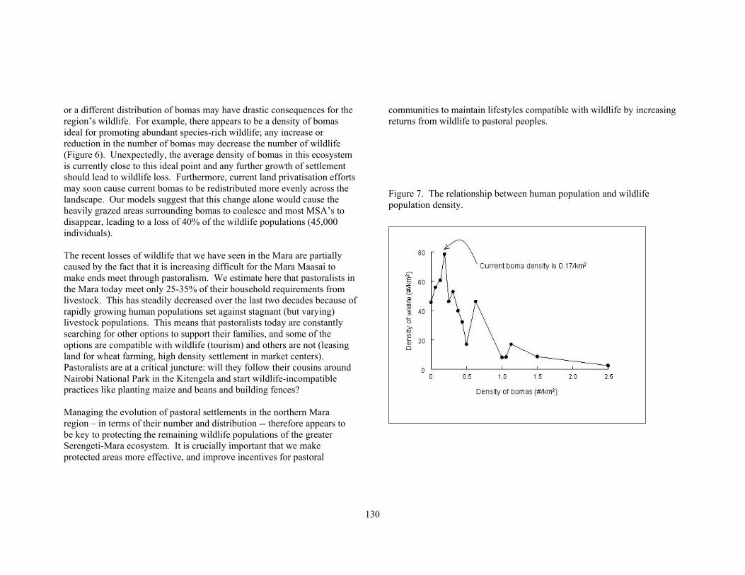
130

or a different distribution of bomas may have drastic consequences for the region’s wildlife. For example, there appears to be a density of bomas ideal for promoting abundant species-rich wildlife; any increase or reduction in the number of bomas may decrease the number of wildlife (Figure 6). Unexpectedly, the average density of bomas in this ecosystem is currently close to this ideal point and any further growth of settlement should lead to wildlife loss. Furthermore, current land privatisation efforts may soon cause current bomas to be redistributed more evenly across the landscape. Our models suggest that this change alone would cause the heavily grazed areas surrounding bomas to coalesce and most MSA’s to disappear, leading to a loss of 40% of the wildlife populations (45,000 individuals). The recent losses of wildlife that we have seen in the Mara are partially caused by the fact that it is increasing difficult for the Mara Maasai to make ends meet through pastoralism. We estimate here that pastoralists in the Mara today meet only 25-35% of their household requirements from livestock. This has steadily decreased over the last two decades because of rapidly growing human populations set against stagnant (but varying) livestock populations. This means that pastoralists today are constantly searching for other options to support their families, and some of the options are compatible with wildlife (tourism) and others are not (leasing land for wheat farming, high density settlement in market centers). Pastoralists are at a critical juncture: will they follow their cousins around Nairobi National Park in the Kitengela and start wildlife-incompatible practices like planting maize and beans and building fences? Managing the evolution of pastoral settlements in the northern Mara region – in terms of their number and distribution -- therefore appears to be key to protecting the remaining wildlife populations of the greater Serengeti-Mara ecosystem. It is crucially important that we make protected areas more effective, and improve incentives for pastoral

communities to maintain lifestyles compatible with wildlife by increasing returns from wildlife to pastoral peoples.

Figure 7. The relationship between human population and wildlife population density.

131

5.3 Further information and discussion needed We think that the following information will help better us understand the patterns we see here and contribute to better management of this valuable wildlife-people system:

• Analysis of trends in wildlife species at a fine resolution from 1989- 2003, using Judy and Mike Rainy’s fine resolution data.

• Analysis of when, where and why multiple species associations of wildlife form and disband.

• Comparison of DRSRS, KWS and Mara Count data to confirm or refute the conclusions here and evaluate the costs and benefits of different monitoring techniques.

• Survey of the number of people per hut in 1999 and 2003 to make an accurate estimate of human populations

• GPS of the reserve boundary in Narok District • Regular counts of all wildlife and livestock species. We suggest

that aerial surveys are conducted 2-3 times a year (in the wet and dry seasons, at least) and ground counts every 2-3 years.

• A better mechanistic understanding of the distribution of wildlife and livestock in relation to environmental and habitat characteristics

• Develop better methods for counting rare species • Better understanding of daily, seasonal and decadenal dynamics

(for example, night distributions and behaviour) • Carnivore monitoring and the spatial associations of carnivores

and prey • Better ways to improve returns to wildlife for all stakeholders,

especially pastoralists • More equitable ways to distribute the returns from wildlife

enterprises • More discussions among individuals and organisations concerned

about the problems of pastoral people and their solutions, and ways for all concerned to join hands to conserve this valuable people-wildlife system

132

6. References Andrews, M. H. 1988. Grazing impacts in relation to livestock watering

points. Trends in Ecology and Evolution 3, 336-339. Bekure, S., de Leeuw, P.N., Grandin, B.E. & Neate, P.J.H. 1991. Maasai

herding: an analysis of the livestock production system of Maasai pastoralists in eastern Kajiado District, Kenya, p. 172. ILCA Systems Study 4. ILCA (International Livestock Centre for Africa), Addis Ababa, Ethiopia.

Bell, R. H. V. 1982. The effect of soil nutrient availability on the community structure in African ecosystems. In: Ecology of tropical savannas. (Eds. B. J. Huntley& B. H. Walker). Springer-Verlag, Berlin, p. 193-216.

Botkin, D. B., Mellio, J. M., and Wu, L. S. 1981. How ecosystem processes are linked to large mammal population dynamics. In: Dynamics of Large Mammal Populations, p. 373-387. Eds. C. W. Fowler and T. D. Smith. Wiley, New York.

Box, G. E. P., and D. R. Cox. 1964. An analysis of transformations. Journal of the Royal Statistical Association, Ser B, 26: 211-243.

Boydston, E.E., Kapheim, K.M., Watts, H.E., Szykman, M. and Holekamp, K.E. 2003. Altered behaviour in spotted hyenas associated with increased human activity. Animal Conservation 6, 1–10.

Boydston, E.E., Kapheim, K.M., Szykman, M. and Holekamp, K.E. 2003. Individual variation in space use by female spotted hyenas Journal of Mammalogy 84(3).

Broten, M. D., and Said, M. 1995. Population trends of ungulates in and around Kenya’s Maasai Mara Reserve. In: Serengeti II: Dynamics, Management and Conservation of an ecosystem. Ed. A. R. E. Sinclair and P, Arcese, p. 169-193. Univ. of Chicago Press, Chicago.

Brown, L.H. 1971. The biology of pastoral man as a factor in conservation. Biological Conservation. 3, 93-100.

Burnham, K.P., and D. R. Anderson. 1998. Model Selection and Inference: A Practical Information-Theoretic Approach. Springer Verlag.

Charnov, E. L. 1976. Optimal foraging: the marginal value theorem. Theoretical Population Biology 9, 129-136.

Cleveland, W.S. 1979. Robust locally weighted regression and smoothing scatterplots. Journal of the American Statistical Association 74: 829-836.

Cleveland, W. S., and S. J. Devlin. 1988. Locally weighted regression: An approach to regression analysis by local fitting. Journal of the American Statistical Association 83: 596-610.

Cleaveland, W. S., S. J. Devlin, and E. Grosse. 1988. Regression by local fitting. Journal of Econometrics 37: 87-114.

Coe, M. J., Cumming, D. H., and Phillipson, J. 1976. Biomass and production of large African herbivores in relation to rainfall and primary production. Oecologia, 22, 341-54.

Cressie, N. A. C. 1991. Statistics for spatial data. Wiley, New York. Cressie, N. A. C., and D. M. Hawkins. 1980. Robust estimation of the

variogram, I. Journal of the International Association of Mathematical Geologists 12: 115-125.

Dawson, J. B. 1963. Carbonatitic volcanic ashes in northern Tanganyika. Bulletin Volcanologique 27, 1-11.

Demment, M. W., and Van Soest, P. 1985. A nutritional explanation for body size patterns of ruminant and non-ruminant herbivores. American Naturalist 125, 641-672.

Dublin, H. T., Sinclair, A. R. R., and McGlade, J. 1990. Elephants and fire as causes of multiple stable states in the Serengeti-Mara woodlands. Journal of Animal Ecology, 59, 1147-1164.

133

Dublin, H.T. 1995. Vegetation dynamics in the Serengeti-Mara ecosystem. The role of elephants, fire, and other factors. In: Serengeti II. Dynamics, management, and Conservation of an ecosystem. Ed. A.R.E. Sinclair & P. Arcese, p. 117-145. University of Chicago Press, Chicago.

East, R. (1984) Rainfall, soil nutrients status and biomass of large African savanna mammals. Afican Journal of Ecology, 22, 245-270.

ESRI Inc. (2000). ArcView Spatial Analyst, version 3.2a. Environmental Systems Research Institute Inc. Redlands, CA, USA.

Estes, R. D. 1991. The behaviour guide to African mammals. University of California Press, London, UK.

Fritz, H., & Duncan, P. 1994. On the carrying capacity for large ungulates of African savanna ecosystems. Proc. Royal Soc. Lond., B, 256, 77-82.

Fryxell, J., Greever, M. J., and Sinclair, A. R. E. 1988. Why are migratory ungulates so abundant? American Naturalist 131, 781-798.

Gotway, C. A., and Stroup, W.W. 1997. A generalized linear model approach to spatial data analysis and prediction. Journal of Agricultural, Biological and Environmental statistics, 2, 157-178.

Grandin, B.E. 1988. Wealth and pastoral dairy production. A case study from Maasailand. Human Ecology. 16, 1-21.

Hanby, J. P., Bygott, J. D., & Packer, C. 1995. Ecology, demography, and behaviour of lions in two contrasting habitats: Ngorongoro Crater and the Serengeti Plains. In: Serengeti II: Dynamics, Management, and Conservation of an Ecosystem, p. 315-331. Eds. A. R. E. Sinclair and P. Arcese. Univ. of Chicago Press, Chicago.

Harrington, R., Owen-Smith, R. N., Viljoen, P. C., Biggs, H. C., Mason, D. R., and Funston, P. 1999. Establishing the causes of the roan antelope decline in the Kruger National Park, South Africa. Biological Conservation 90: 69-78.

Herlocker, D. J. 1992. Vegetation types. In: Range Management Handbook of Kenya, Vol 2:Samburu District. Eds. S. B. Shaabani,

M, Walsh, D. J. Herlocker and D. Walther. Nairobi, Kenya: Republick of Kenya, Ministry of Livestock Development.

Homewood, K.M. & Rodgers, W.A. 1991. Maasailand ecology: pastoral development and wildlife conservation in Ngorongoro, Tanzania, p 298. Cambridge University Press.

Homewood K., Lambin E.F., Coast E., Kariuki A., Kikula I., Kivelia J., Said M., Serneels S. & Thompson M. 2001. Long-term changes in Serengeti-Mara wildebeest and land cover: pastoralism, population, or policies? Proceedings of the National Academy of Sciences, USA. 98 (22), 12,544-12,549.

Hurvich, C. M., and Simonoff, J. S. 1998. Smoothing parameter selection in non-parametric regression using an improved Akaike Information Criterion. Journal of the Royal Statistical Society B 60: 271-293.

Jackman, H. 2002. Comparison of aerial counts with ground counts for large African herbivores. Journal of Applied Ecology, 39, 841-852.

Jarman, P. J. 1974. The social organisation of antelope in relation to their ecology. Behaviour 48, 215-266.

Jewell, P.A. 1980. Ecology and management of game animals and domestic livestock in African savannas. Human Ecology in Savannah Environments (ed. by D.R. Harris), pp. 353-382. Academic Press, New York.

Journel, A. G., and Huijbretgs, C. J. 1978. Mining geostatistics. Academic Press, London.

Krebs, J. R. 1978. Optimal foraging: decision rules for predators. In: Behavioural Ecology. Eds. J. R. Krebs and N. B. Davis. Blackwell Scientific Publications, Oxford.

Kruuk, H. 1972. The spotted hynena: A study of predation and social behaviour. University of Chicago Press, Chicago.

134

Lamprey, R.H. 1984. Maasai impact on Kenya savanna vegetation: a remote sensing approach. PhD Thesis, University of Aston-in-Birmingham, UK.

Lamprey, R.H. and Michelmore, F. 1996. The wildlife protected areas of Uganda. EC Wildlife Project, Ministry of Tourism, Wildlife and Antiquities, Kampala, Uganda.

Lamprey, R.H. and Reid, R.S. Expansion of settlement in Maasai Mara, Kenya: what future for pastoralism and conservation. Journal of Biogeography (submitted)

Leakey, M.D. & Hay, R.L. 1979. Pliocene footprints in the Laetolil beds at Laetoli, northern Tanzania. Nature 278: 317-323.

Maddock, L. 1979. The “migration” and grazing succession. In: Serengeti: Dynamics of an ecosystem, p. 104-129. Eds. A. R. E. Sinclair and M, Norton-Griffiths. Univ. of Chicago Press, Chicago.

Marshall, F. in Early Pastoralists of South-western Kenya, Memoir 11 (ed, Robertshaw, P.) British Institute in Eastern Africa, Nairobi, Kenya, 1990.

McCabe, J.T., Schofield, E.C., Nygaard Pedersen G., Lekule, A. & Tumaini, A. 1997. Food security and nutritional status. Multiple land-use: the experience of the Ngorongoro Conservation Area, Tanzania (ed. by D.M. Thompson), pp. 285-302. IUCN, Gland, Switzerland and Cambridge, UK.

McNaughton, S. J. 1979. Grassland-herbivore dysnamics. In: Serengeti. Dynamics of an ecosystem, p. 46-86. Eds. A. R. E. Sinclair and M, Norton-Griffiths. Univ. of Chicago Press, Chicago.

McNaughton, S. J. 1983. Serengeti grassland ecology: the role of composite environmental factors and contingency in community organization. Ecoogical Monographs 53: 291-320.

McNaughton, S. J. 1985. Ecology of a grazing system: The Serengeti. Ecological Monographs 55: 259-294.

McNaughton, S. J. 1988. Mineral nutrition and spatial concentration of African ungulates. Nature, 334, 343-345.

McNaughton, S. J., Ruess, R. W., Seagle, S. W. 1988. Large mammals and process dynamics in African ecosystems: herbivorous mammals affect primary productivity and regulate recycling balances. Bioscience 38, 794-800.

McNaughton, S. J. 1990. Mineral nutrition and seasonal movements of African migratory ungulates. Nature, 345, 613-615.

McNaughton, S. J., and Georgiadis, N. J. 1986. Ecology of African grazing and browsing mammals. Ann. Rev. Ecol. Syst. 17, 39-65.

McNaughton, S. J., Banyikwa, F. F., and M. M. McNaughton. 1997. Promotion of the cycling of diet-enhancing nutrients by African grazers. Science 278, 1798-1800.

Mduma, S.A.R., Sinclair, A.R.E & Hilborn, R. 1999. Food regulates the Serengeti wildebeest: a 40-year record. Journal of Animal Ecology, 68, 1101-1122.

Mduma 2000 Morrison, C. G. T., Hoyle, A.C., and Hope-Simpson. 1948. Tropical soil

vegetation catenas and mosaics. J. Ecol. 36, 1-48. Muchiru, A.N. 1992 The ecological impact of abandoned Maasai

settlements on savanna vegetation and its herbivores in the Amboseli ecosystem, MSc thesis. University of Nairobi.

Muchiru, A.N, Western, D.J., Reid, R.S. The role of abandoned pastoral settlements in the dynamics of African large herbivore communities. Journal of Applied Ecology (submitted)

Muchiru, A.N, Western, D.J. and Reid, R.S. The impact of abandoned pastoral settlements on plant and nutrient succession in the African savannas. Journal of Applied Ecology (submitted).

NCAA (1999) 1998 aerial boma count, 1999 people and livestock census, and human population trend between 1954 and 1999 in NCA. Research and Planning Unit, Ngorongoro Conservation Area Authority, Tanzania.

Norton-Griffiths, M. 1995. Economic incentives to develop rangelands of the Serengeti: Implications for wildlife conservation. In Serengeti

135

II: Dynamics, Management and Conservation of an ecosystem. Ed. A. R. E. Sinclair and P, Arcese, p. 588-604. Univ. of Chicago Press, Chicago.

O'Connell, M., and R. D. Wolfinger. 1997. Spatial Regression Models, Response Surfaces, and Process Optimization. Journal of Computational and Graphical Statistics, 6: 224-241.

Ogutu, J. O. 2000. Herbivore dynamics in the Mara Area of Kenya: The effects of land use, climate and predators. Shaker Verlag, Aachen, Germany.

Otichillo, W. K., De Leeuw, J., Skidmore, A. K., Prins, H. H. T., and Said, M. 2000. Population trends of large non-migratory wild herbivores and livestock in the Mara ecosystem, Kenya, between 1977 and 1997. African Journal of Ecology 38: 202-216.

Owen-Smith, N. 1982. Factors influencing the consumption of plant products by large herbivores. In: Ecology of tropical Savannas, 359-404. Eds. B. J. Huntley and B. H. Walker. Ecological Studies 42, Springer Verlag, Berlin.

Owen-Smith, N., and Novellie, P. 1982. What should a clever ungulate eat? American Naturalist 119, 151-178.

Owen-Smith, N. 1988. Megaherbivores: the influence of very large body size on ecology. Cambridge University Press, Cambridge.

Owen-Smith, N. 1996. Ecological guidelines for waterpoints in extensive protected areas. South African Journal of Wildlife Research 26, 107-112.

Packer, C. 1986. The ecology of sociality in felids. In: Ecological aspects of social evolution. Ed. D. I. Rubinstein and R. W. Wrangham. Princeton: Princeton University Press.

Pennycuick, L. 1975. Movements of migratory wildebeest population in the Serengeti Area between 1960 and 1973. E. Afr. Wildl. J., 13, 65-87.

Pennycuick, L., & Norton-Griffiths, M. (1976) Fluctuations in the rainfall of the Serengeti ecosystem, Tanzania. J. Biogeogr., 3, 125-40.

Pellew, R. 1983. The impacts of elephant, giraffe, and fire upon the Acacia tortilis woodlands of the Serengeti. Afr. J. Ecol. 21, 41-71.

Pickering, R., & Harfum, J. R. 1961. Stratigraphy. 14. Stratigraphical nomenclature of the Bukoban rocks in the Musoma district and on the Western Serengeti. Records of the Geological Survey of Tanganyika, 9, 76-80.

Pratt, D.J. & Gwynne, M.D. (eds) 1977. Rangeland management and ecology in East Africa, p. 310. Hodder and Stoughton, London.

Prins, H. H. T. 1996. Ecology and behaviour of the African Buffalo. Chapman and Hall, London, UK.

Redfern J. V., Grant, C. C., Biggs, H. C., and W. M. Getz, in press. Constrained foraging and the distribution of herbivores with respect to water in Kruger National Park. Ecology.

Rainy, M. & Rainy, J. 1989. High noon on the Maasai Mara. New Scientist 124: 48-53.

Rainy, M.E. and Worden, J.S. 1997. Trends in livestock and wildlife from the 1970’s to 1990’s in Kenya. Unpublished report.

Reid, R.S., Rainy, M.E, Wilson, C.J., Harris, E., Kruska, R.L., Waweru, M.N., Macmillan, S.A. and Worden, J.S. 2001. Wildlife cluster around pastoral settlements in Africa. PLE Science series #2, International Livestock Research Institute, Nairobi, Kenya.

Rossi, R. E., D. J. Mulla, A. G. Journel, and E. H. Franz. 1992. Geostatistical tools for modeling and interpreting ecological spatial dependence. Ecological Monographs, 62: 277-314.

Rutherford, M.C. 1980. Annual plant production-precipitation relations in arid and semi- arid regions. South African Journal of Science 76, 53-56.

Rutherford, M. C. 1984. Relative allocation and seasonal phasing of growth of woody plant components in a South African savanna. Progress in Biometeorology 3, 200-221.

136

Said, M.Y., de Leeuw, J., Skidmore, A.K. and Prins, H.H.T. Coexistence of pastoralism and wildlife in Kenya: moving beyond perception. Biological Conservation (submitted)

SAS Institute Inc. 2001. SAS system for windows, version 8.2. SAS Institute Inc., Carey, NC, USA.

Serneels, S. Said, M. Y. Lambin, E. F. Land-cover changes around a major East African wildlife reserve: the Mara Ecosystem (Kenya) International Journal of Remote Sensing 22(17), 3397-3420.

Schaller, G. B. 1972. The Serengeti lion: A study in predator-prey relations Univ. of Chicago Press, Chicago.

Sinclair, A.R.E. 1975. The resource limitation of trophic levels in tropical grassland ecosystems. J. Anim. Ecol., 44, 495-520.

Sinclair, A.R.E. & Arcese, P. 1995. Serengeti in the context of world wide conservation efforts. In: Serengeti II. Dynamics, Management, and conservation of an ecosystem, p.31-46. ed. A.R.E. Sinclair & P.Arcese. University of Chicago Press, Chicago.

Smuts, G. L. 1978. Interrelationships between predators, prey and their environment. Bioscience, 28, 316-320.

Stelfox, J. G., Peden, D.G., Epp, H., Hudson, R. J., Mbugwa, S. W., Agatsiva, J. L., and Amunyunzu, C. L. 1986. J. Wildl. Manage., 50, 339-347.

Thompson, D.M., and Homewood, K.M. 2002. Entrepreneurs, elites and exclusion in Maasailand. Human Ecology 30 (1): 107-138.

Thornton, P.K., Kruska, R.L., Henninger, N., Kristjanson, P.M., Reid, R.S., Atieno, F., Odero, A.N. and Ndegwa, T. 2002. Mapping poverty and livestock in the developing world. ILRI (International Livestock Research Institute), Nairobi, Kenya. 124 pages.

Thrash, I., and Derry, J. F. 1999. The nature and modeling of piospheres: a review. Koedoe 42, 73-94.

Thurston, W. S., Wand, M. P., and Wiencke, J. K. 2000. Negative binomial additive models. Biometrics 56, 139-144.

Van Orsdol, K. G., Hanby, J. P., & Bygott, J. D. 1985. Ecological correlates of lion social organization. J. Zool. (Lond.), 206, 97-112.

Vesey-Fitzegerald, D. F. 1965. The utilization of natural pastures by wild animals in the Rukwa Valley, Tanganyika. East African Wildlife Journal 3, 38-48.

Walker, B. H. R., and I. Noy-Meir. 1982. Aspects of the stability and resilience of savanna ecosystems. In: Ecology of tropical Savannas, p. 556-590. Eds. B. J. Huntley and B. H. Walker. Ecological Studies 42, Springer Verlag, Berlin.

Walker, B. H., Emslie, R. H., Owen-Smith, R. N., and Scholes, R. J. 1987. To cull or not to cull: lessons from a Southern African drought. Journal of Applied Ecology 24, 381-401.

Western, D. 1975. Water availability and its influence on the structure and dynamics of a large mammal community. East African Wildlife Journal, 13, 265-286.

Williams, L. A. J. 1966. An ecological survey of the Narok District of Kenya Masailand, 1961-1965. Part I. In: Geology, p. 7-14 (ED, P. E. Glover). Conservation Foundation, New York, USA.

Williams, S. D. 1998. Grevy’s zebra: ecology in a heterogeneous environment. PhD thesis University of London, 1999 pp.

Worden, J.S., Reid, R.S. and Gichohi, H. 2003. Land-use effects on large wildlife and livestock in the Greater Amboseli swamps. LUCID working paper, ILRI, Nairobi, Kenya.

Young, T.P., Patridge, N. & Macrae, A. (1995) Long-term glades in Acacia bushland and their edge effects in Laikipia, Kenya. Ecological Applications, 5(1), 97-108.

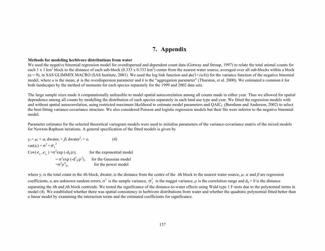
137

7. Appendix Methods for modeling herbivore distributions from water We used the negative binomial regression model for overdispersed and dependent count data (Gotway and Stroup, 1997) to relate the total animal counts for each 1 x 1 km2 block to the distance of each sub-block (0.333 x 0.333 km2) center from the nearest water source, averaged over all sub-blocks within a block (n = 9), in SAS GLIMMIX MACRO (SAS Institute, 2001). We used the log link function and φu(1+(u/k)) for the variance function of the negative binomial model, where u is the mean, φ is the overdispersion parameter and k is the “aggregation parameter” (Thurston, et al. 2000). We estimated a common k for both landscapes by the method of moments for each species separately for the 1999 and 2002 data sets. The large sample sizes made it computationally unfeasible to model spatial autocorrelation among all counts made in either year. Thus we allowed for spatial dependence among all counts by modelling the distribution of each species separately in each land use type and year. We fitted the regression models with and without spatial autocorrelation, using restricted maximum likelihood to estimate model parameters and QAICC (Burnham and Anderson, 2002) to select the best-fitting variance-covariance structure. We also considered Poisson and logistic regression models but their fits were inferior to the negative binomial model. Parameter estimates for the selected theoretical variogram models were used to initialise parameters of the variance-covariance matrix of the mixed models for Newton-Raphson iterations. A general specification of the fitted models is given by yi = µi + αi dwateri + βi dwater2

i + ei (4) var(ei) = σ2 + 2

1σ Cov(

21, ii ee ) =σ2exp (-dij/ρ), for the exponential model

= σ2exp (-d2ij/ρ2), for the Gaussian model

=σ2ρdij, for the power model

where yi is the total count in the ith block, dwateri is the distance from the centre of the ith block to the nearest water source, µ, α and β are regression coefficients, ei are unknown random errors, σ2 is the sample variance, 2

1σ is the nugget variance, ρ is the correlation range and dij > 0 is the distance separating the ith and jth block centroids. We tested the significance of the distance-to-water effects using Wald type 1 F-tests due to the polynomial terms in model (4). We established whether there was spatial consistency in herbivore distributions from water and whether the quadratic polynomial fitted better than a linear model by examining the interaction terms and the estimated coefficients for significance.

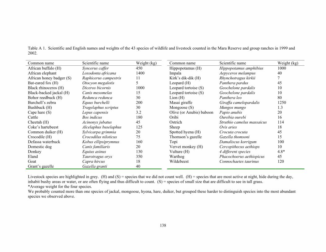
138

Table A 1. Scientific and English names and weights of the 43 species of wildlife and livestock counted in the Mara Reserve and group ranches in 1999 and 2002. Common name Scientific name Weight (kg) Common name Scientific name Weight (kg) African buffalo (H) Syncerus caffer 450 Hippopotamus (H) Hippopotamus amphibius 1000 African elephant Loxodonta africana 1400 Impala Aepyceros melampus 40 African honey badger (S) Raphicerus campestris 11 Kirk’s dik-dik (H) Rhynchotragus kirkii 7 Bat-eared fox (H) Otocyon megalotis 5 Leopard (H) Panthera pardus 45 Black rhinoceros (H) Diceros bicornis 1000 Leopard tortoise (S) Geochelone pardalis 10 Black-backed jackal (H) Canis mesomelas 15 Leopard tortoise (S) Geochelone pardalis 10 Bohor reedbuck (H) Redunca redunca 30 Lion (H) Panthera leo 80 Burchell’s zebra Equus burchelli 200 Masai giraffe Giraffa camelopardalis 1250 Bushbuck (H) Tragelaphus scriptus 30 Mongoose (S) Mungos mungo 1.3 Cape hare (S) Lepus capensis 3.2 Olive (or Anubis) baboon Papio anubis 20 Cattle Bos indicus 180 Oribi Ourebia ourebi 16 Cheetah (H) Acinonyx jubatus 45 Ostrich Struthio camelus massaicus 114 Coke’s hartebeest Alcelaphus buselaphus 125 Sheep Ovis aries 18 Common duiker (H) Sylvicarpa grimmia 20 Spotted hyena (H) Crocuta crocuta 45 Crocodile (H) Crocodilus niloticus 75 Thomson’s gazelle Gazella thomsoni 15 Defassa waterbuck Kobus ellipsiprymnus 160 Topi Damaliscus korrigum 100 Domestic dog Canis familiaris 20 Vervet monkey (H) Cercopithecus aethiops 10 Donkey Equius asinus 130 Vulture (H) 4 different species 4.8* Eland Taurotragus oryx 350 Warthog Phacochoerus aethiopicus 45 Goat Capra hircus 18 Wildebeest Connochaetes taurinus 120 Grant’s gazelle Gazella granti 40 Livestock species are highlighted in grey. (H) and (S) = species that we did not count well. (H) = species that are most active at night, hide during the day, inhabit bushy areas or water, or are often flying and thus difficult to count. (S) = species of small size that are difficult to see in tall grass. *Average weight for the four species. We probably counted more than one species of jackal, mongoose, hyena, hare, duiker, but grouped these harder to distinguish species into the most abundant species we observed above.

Table A 2. Number of animals counted by each ground counting team during November 2002. Area and species ↓ Team 1 2 3 4 5 6 7 8 9 10 11 12 13 14 15 16 17 18 19 20 X all TotalArea covered (km2) 119.7 207.7 39.0 99.8 93.7 134.6 79.2 121.0 122.4 110.8 116.7 95.0 91.1 53.1 80.2 115.2 109.9 154.7 68.7 72.6 68.7 58.8 2,212.3Cattle 0 0 0 2,689 2,919 1,945 300 4,982 0 0 1,306 4,894 2,048 947 1,445 6,523 1,510 4,823 3,334 3,264 0 2,104 45,033Donkey 0 0 0 0 6 7 0 25 0 0 0 11 28 8 21 7 40 20 88 13 0 29 303Sheep & goats 0 0 0 950 2,232 2,249 0 6,891 0 0 0 6,304 3,512 2,251 3,705 4,107 3,149 7,915 9,906 1,970 0 4,553 59,694Domestic dog 0 0 0 9 36 20 0 34 0 0 0 9 19 8 19 3 29 32 57 37 0 37 349Baboon 18 68 0 98 116 77 181 25 31 157 0 52 444 28 3 71 0 31 89 96 14 96 1,695Bat-eared fox 0 9 2 0 2 0 2 0 0 0 0 0 5 2 3 3 0 0 2 1 1 7 39Buffalo 17 810 0 586 5 67 262 0 404 32 107 8 35 0 0 31 139 11 0 41 3 3 2,561Bushbuck 0 40 0 1 2 0 0 1 0 3 0 2 0 0 1 3 3 0 0 3 6 0 65Crocodile 0 0 0 0 6 4 0 0 0 5 0 0 1 0 0 0 0 0 0 0 0 0 16Cheetah 1 0 0 2 0 0 0 0 0 4 0 0 2 0 0 1 5 2 0 0 0 0 17Dikdik 0 2 0 5 2 0 0 13 0 1 0 15 23 5 10 5 13 5 53 80 0 8 240Duiker 0 1 0 0 0 0 2 0 5 0 0 0 0 0 0 0 0 1 0 0 0 0 9Eland 21 85 0 137 11 32 29 4 216 478 74 8 3 9 0 143 48 39 5 0 72 31 1,445Elephant 29 66 109 41 0 0 22 5 114 77 112 42 17 0 7 28 31 33 48 9 30 0 820Giraffe 15 33 0 101 11 30 13 57 42 53 12 57 139 54 22 48 20 93 27 43 0 10 880Grant's gazelle 21 154 0 317 88 286 229 87 254 103 236 337 448 235 291 487 182 160 554 201 62 184 4,916Honey badger 0 0 0 0 0 10 0 0 0 0 14 0 0 0 0 0 0 0 0 0 0 1 25Hippopotamus 0 57 4 0 54 7 91 0 2 255 0 0 0 0 0 0 0 0 44 0 0 1 515Hare 0 0 0 2 1 7 1 1 0 2 0 1 1 3 1 1 4 1 13 9 1 1 50Hyena 4 23 1 9 16 22 23 0 20 28 5 22 18 0 7 4 3 8 7 0 7 24 251Hartebeest 15 34 0 38 18 25 2 6 41 42 32 10 25 28 5 87 67 24 3 42 66 7 617Impala 584 1,010 44 811 1,698 796 537 967 253 1,351 289 849 2,309 830 860 883 238 1,355 2,156 1,147 231 439 19,637Jackal 9 4 0 11 4 7 14 1 4 5 2 8 13 11 11 15 7 9 3 1 9 11 159Lion 6 4 2 19 15 2 4 3 12 18 3 20 0 0 0 8 0 2 4 5 25 17 169Leopard 0 0 0 0 0 0 0 0 0 1 0 0 0 0 0 0 0 0 0 1 0 0 2Mongoose 83 75 11 92 112 53 66 1 102 71 33 57 103 24 0 34 41 7 49 36 13 25 1,088Oribi 8 72 33 6 0 0 3 0 0 0 0 0 0 0 0 0 0 0 0 0 0 0 122Ostrich 7 5 0 6 2 27 15 28 17 39 29 6 6 13 7 20 1 15 0 8 82 6 339Reedbuck 33 16 0 8 0 3 37 0 35 32 7 0 0 0 0 6 3 0 0 0 20 0 200Rhinoceros 0 0 0 0 0 0 0 1 8 2 0 0 0 0 0 0 0 0 0 0 0 0 11Thomson's gazelle 5,771 2,903 526 3,066 3,539 3,355 2,697 1,127 931 2,136 1,378 1,827 4,000 1,440 2,263 2,818 1,560 3,588 1,012 679 1,320 2,797 50,733Topi 255 694 93 494 498 627 621 229 232 603 369 224 795 183 160 438 149 334 112 196 83 312 7,701Tortoise 0 0 1 2 3 2 1 0 1 8 4 2 5 0 2 3 2 1 1 9 7 0 54Vulture 51 218 49 26 1 27 45 18 126 229 87 38 73 24 5 77 1 13 100 25 74 41 1,348Vervet 45 0 0 7 10 6 0 16 1 9 1 0 117 8 23 1 30 21 0 29 98 0 422Waterbuck 67 82 22 127 0 120 77 63 21 60 5 2 4 4 0 9 20 29 15 7 0 2 736Warthog 137 143 4 320 46 241 273 31 168 190 43 36 142 26 17 57 25 170 32 60 82 26 2,269Wildebeest 24,513 21,483 1,436 978 4,901 767 503 157 24,762 10,844 25,133 581 1,313 500 1,720 15,608 799 2,278 371 262 8,710 6,466154,085Zebra 4,480 4,755 220 2,587 3,851 1,592 429 216 1,901 2,069 6,557 1,082 1,961 330 517 2,213 658 980 284 223 769 1,284 38,958Total 36,310 33,054 2,596 13,645 20,299 12,548 6,558 15,110 29,825 19,018 35,955 16,599 17,700 7,024 11,205 33,857 8,887 22,155 18,438 8,570 11,854 18,581399,685

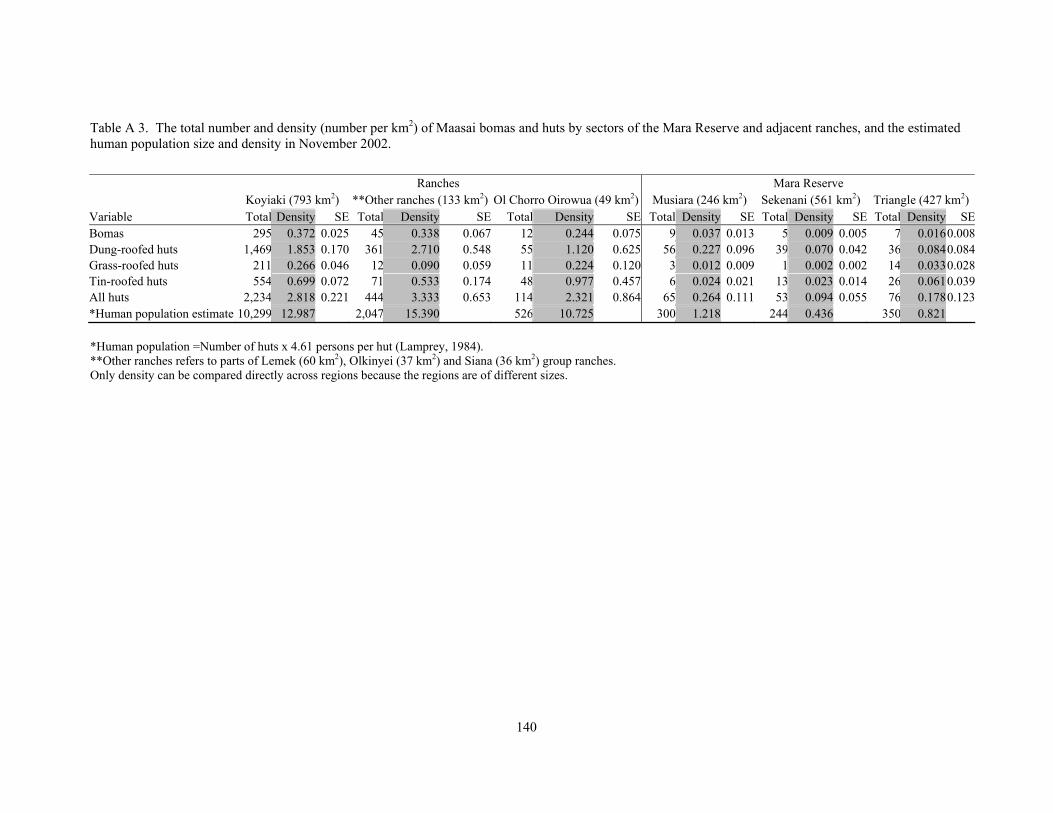
140

Table A 3. The total number and density (number per km2) of Maasai bomas and huts by sectors of the Mara Reserve and adjacent ranches, and the estimated human population size and density in November 2002.

Ranches Mara Reserve Koyiaki (793 km2) **Other ranches (133 km2) Ol Chorro Oirowua (49 km2) Musiara (246 km2) Sekenani (561 km2) Triangle (427 km2)Variable Total Density SE Total Density SE Total Density SE Total Density SE Total Density SE Total Density SEBomas 295 0.372 0.025 45 0.338 0.067 12 0.244 0.075 9 0.037 0.013 5 0.009 0.005 7 0.0160.008Dung-roofed huts 1,469 1.853 0.170 361 2.710 0.548 55 1.120 0.625 56 0.227 0.096 39 0.070 0.042 36 0.0840.084Grass-roofed huts 211 0.266 0.046 12 0.090 0.059 11 0.224 0.120 3 0.012 0.009 1 0.002 0.002 14 0.0330.028Tin-roofed huts 554 0.699 0.072 71 0.533 0.174 48 0.977 0.457 6 0.024 0.021 13 0.023 0.014 26 0.0610.039All huts 2,234 2.818 0.221 444 3.333 0.653 114 2.321 0.864 65 0.264 0.111 53 0.094 0.055 76 0.1780.123*Human population estimate 10,299 12.987 2,047 15.390 526 10.725 300 1.218 244 0.436 350 0.821 *Human population =Number of huts x 4.61 persons per hut (Lamprey, 1984). **Other ranches refers to parts of Lemek (60 km2), Olkinyei (37 km2) and Siana (36 km2) group ranches. Only density can be compared directly across regions because the regions are of different sizes.

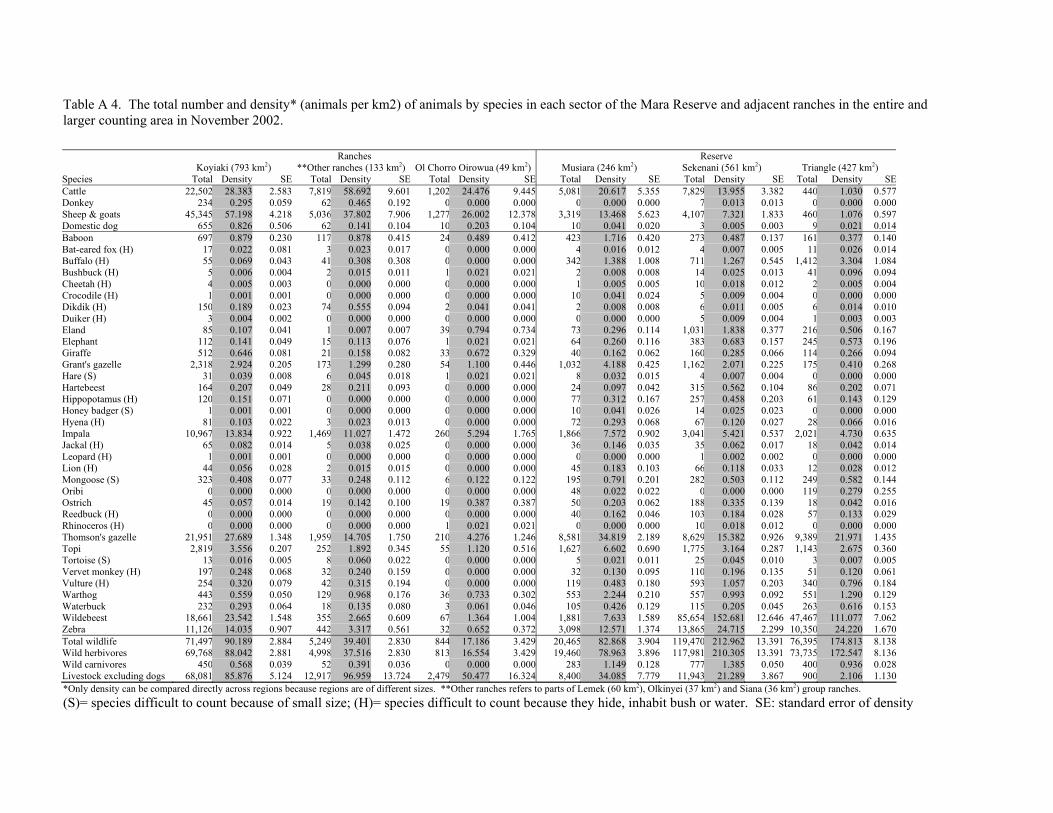
Table A 4. The total number and density* (animals per km2) of animals by species in each sector of the Mara Reserve and adjacent ranches in the entire and larger counting area in November 2002. Ranches Reserve Koyiaki (793 km2) **Other ranches (133 km2) Ol Chorro Oirowua (49 km2) Musiara (246 km2) Sekenani (561 km2) Triangle (427 km2) Species Total Density SE Total Density SE Total Density SE Total Density SE Total Density SE Total Density SECattle 22,502 28.383 2.583 7,819 58.692 9.601 1,202 24.476 9.445 5,081 20.617 5.355 7,829 13.955 3.382 440 1.030 0.577Donkey 234 0.295 0.059 62 0.465 0.192 0 0.000 0.000 0 0.000 0.000 7 0.013 0.013 0 0.000 0.000Sheep & goats 45,345 57.198 4.218 5,036 37.802 7.906 1,277 26.002 12.378 3,319 13.468 5.623 4,107 7.321 1.833 460 1.076 0.597Domestic dog 655 0.826 0.506 62 0.141 0.104 10 0.203 0.104 10 0.041 0.020 3 0.005 0.003 9 0.021 0.014Baboon 697 0.879 0.230 117 0.878 0.415 24 0.489 0.412 423 1.716 0.420 273 0.487 0.137 161 0.377 0.140Bat-eared fox (H) 17 0.022 0.081 3 0.023 0.017 0 0.000 0.000 4 0.016 0.012 4 0.007 0.005 11 0.026 0.014Buffalo (H) 55 0.069 0.043 41 0.308 0.308 0 0.000 0.000 342 1.388 1.008 711 1.267 0.545 1,412 3.304 1.084Bushbuck (H) 5 0.006 0.004 2 0.015 0.011 1 0.021 0.021 2 0.008 0.008 14 0.025 0.013 41 0.096 0.094Cheetah (H) 4 0.005 0.003 0 0.000 0.000 0 0.000 0.000 1 0.005 0.005 10 0.018 0.012 2 0.005 0.004Crocodile (H) 1 0.001 0.001 0 0.000 0.000 0 0.000 0.000 10 0.041 0.024 5 0.009 0.004 0 0.000 0.000Dikdik (H) 150 0.189 0.023 74 0.555 0.094 2 0.041 0.041 2 0.008 0.008 6 0.011 0.005 6 0.014 0.010Duiker (H) 3 0.004 0.002 0 0.000 0.000 0 0.000 0.000 0 0.000 0.000 5 0.009 0.004 1 0.003 0.003Eland 85 0.107 0.041 1 0.007 0.007 39 0.794 0.734 73 0.296 0.114 1,031 1.838 0.377 216 0.506 0.167Elephant 112 0.141 0.049 15 0.113 0.076 1 0.021 0.021 64 0.260 0.116 383 0.683 0.157 245 0.573 0.196Giraffe 512 0.646 0.081 21 0.158 0.082 33 0.672 0.329 40 0.162 0.062 160 0.285 0.066 114 0.266 0.094Grant's gazelle 2,318 2.924 0.205 173 1.299 0.280 54 1.100 0.446 1,032 4.188 0.425 1,162 2.071 0.225 175 0.410 0.268Hare (S) 31 0.039 0.008 6 0.045 0.018 1 0.021 0.021 8 0.032 0.015 4 0.007 0.004 0 0.000 0.000Hartebeest 164 0.207 0.049 28 0.211 0.093 0 0.000 0.000 24 0.097 0.042 315 0.562 0.104 86 0.202 0.071Hippopotamus (H) 120 0.151 0.071 0 0.000 0.000 0 0.000 0.000 77 0.312 0.167 257 0.458 0.203 61 0.143 0.129Honey badger (S) 1 0.001 0.001 0 0.000 0.000 0 0.000 0.000 10 0.041 0.026 14 0.025 0.023 0 0.000 0.000Hyena (H) 81 0.103 0.022 3 0.023 0.013 0 0.000 0.000 72 0.293 0.068 67 0.120 0.027 28 0.066 0.016Impala 10,967 13.834 0.922 1,469 11.027 1.472 260 5.294 1.765 1,866 7.572 0.902 3,041 5.421 0.537 2,021 4.730 0.635Jackal (H) 65 0.082 0.014 5 0.038 0.025 0 0.000 0.000 36 0.146 0.035 35 0.062 0.017 18 0.042 0.014Leopard (H) 1 0.001 0.001 0 0.000 0.000 0 0.000 0.000 0 0.000 0.000 1 0.002 0.002 0 0.000 0.000Lion (H) 44 0.056 0.028 2 0.015 0.015 0 0.000 0.000 45 0.183 0.103 66 0.118 0.033 12 0.028 0.012Mongoose (S) 323 0.408 0.077 33 0.248 0.112 6 0.122 0.122 195 0.791 0.201 282 0.503 0.112 249 0.582 0.144Oribi 0 0.000 0.000 0 0.000 0.000 0 0.000 0.000 48 0.022 0.022 0 0.000 0.000 119 0.279 0.255Ostrich 45 0.057 0.014 19 0.142 0.100 19 0.387 0.387 50 0.203 0.062 188 0.335 0.139 18 0.042 0.016Reedbuck (H) 0 0.000 0.000 0 0.000 0.000 0 0.000 0.000 40 0.162 0.046 103 0.184 0.028 57 0.133 0.029Rhinoceros (H) 0 0.000 0.000 0 0.000 0.000 1 0.021 0.021 0 0.000 0.000 10 0.018 0.012 0 0.000 0.000Thomson's gazelle 21,951 27.689 1.348 1,959 14.705 1.750 210 4.276 1.246 8,581 34.819 2.189 8,629 15.382 0.926 9,389 21.971 1.435Topi 2,819 3.556 0.207 252 1.892 0.345 55 1.120 0.516 1,627 6.602 0.690 1,775 3.164 0.287 1,143 2.675 0.360Tortoise (S) 13 0.016 0.005 8 0.060 0.022 0 0.000 0.000 5 0.021 0.011 25 0.045 0.010 3 0.007 0.005Vervet monkey (H) 197 0.248 0.068 32 0.240 0.159 0 0.000 0.000 32 0.130 0.095 110 0.196 0.135 51 0.120 0.061Vulture (H) 254 0.320 0.079 42 0.315 0.194 0 0.000 0.000 119 0.483 0.180 593 1.057 0.203 340 0.796 0.184Warthog 443 0.559 0.050 129 0.968 0.176 36 0.733 0.302 553 2.244 0.210 557 0.993 0.092 551 1.290 0.129Waterbuck 232 0.293 0.064 18 0.135 0.080 3 0.061 0.046 105 0.426 0.129 115 0.205 0.045 263 0.616 0.153Wildebeest 18,661 23.542 1.548 355 2.665 0.609 67 1.364 1.004 1,881 7.633 1.589 85,654 152.681 12.646 47,467 111.077 7.062Zebra 11,126 14.035 0.907 442 3.317 0.561 32 0.652 0.372 3,098 12.571 1.374 13,865 24.715 2.299 10,350 24.220 1.670Total wildlife 71,497 90.189 2.884 5,249 39.401 2.830 844 17.186 3.429 20,465 82.868 3.904 119,470 212.962 13.391 76,395 174.813 8.138Wild herbivores 69,768 88.042 2.881 4,998 37.516 2.830 813 16.554 3.429 19,460 78.963 3.896 117,981 210.305 13.391 73,735 172.547 8.136Wild carnivores 450 0.568 0.039 52 0.391 0.036 0 0.000 0.000 283 1.149 0.128 777 1.385 0.050 400 0.936 0.028Livestock excluding dogs 68,081 85.876 5.124 12,917 96.959 13.724 2,479 50.477 16.324 8,400 34.085 7.779 11,943 21.289 3.867 900 2.106 1.130*Only density can be compared directly across regions because regions are of different sizes. **Other ranches refers to parts of Lemek (60 km2), Olkinyei (37 km2) and Siana (36 km2) group ranches. (S)= species difficult to count because of small size; (H)= species difficult to count because they hide, inhabit bush or water. SE: standard error of density

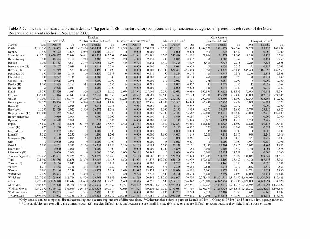
Table A 5. The total biomass and biomass density* (kg per km2, SE= standard error) by species and by functional categories of species in each sector of the Mara Reserve and adjacent ranches in November 2002. Ranches Mara Reserve Koyiaki (793 km2) **Other ranches (133 km2) Ol Chorro Oirowua (49 km2) Musiara (246 km2) Sekenani (561km2) Triangle (427 km2) Species Total Density SE Total Density SE Total Density SE Total Density SE Total Density SE Total Density SECattle 4,050,360 5,109.073 464.935 1,407,420 10564.454 1728.142 216,360 4405.521 1700.057 914,580 3711.101 963.968 1,409,220 2511.978 608.768 79,200 185.335 103.889Donkey 30,420 38.372 7.619 8,060 60.501 24.943 0 0.000 0.000 0 0.000 0.000 910 1.622 1.622 0 0.000 0.000Sheep & goats 816,210 1,029.557 75.936 90,648 680.427 142.298 22,986 468.041 222.801 59,742 242.416 101.218 73,926 131.775 33.005 8,280 19.376 10.736Domestic dog 13,100 16.524 10.112 1,240 9.308 2.096 200 4.073 2.070 200 0.812 0.397 60 0.107 0.062 180 0.421 0.269Baboon 13,940 17.583 4.607 2,340 17.564 8.294 480 9.774 8.242 8,460 34.328 8.409 5,460 9.733 2.735 3,220 7.535 2.805Bat-eared fox (H) 85 0.107 0.040 15 0.113 0.084 0 0.000 0.000 20 0.081 0.058 20 0.036 0.022 55 0.129 0.068Buffalo (H) 24,750 31.219 19.571 18,450 138.490 138.490 0 0.000 0.000 153,900 624.481 453.418 319,950 570.321 245.485 635,400 1,486.895 487.559Bushbuck (H) 150 0.189 0.100 60 0.450 0.319 30 0.611 0.611 60 0.244 0.244 420 0.749 0.371 1,230 2.878 2.809Cheetah (H) 180 0.227 0.139 0 0.000 0.000 0 0.000 0.000 45 0.183 0.183 450 0.802 0.520 90 0.211 0.149Crocodile (H) 75 0.095 0.095 0 0.000 0.000 0 0.000 0.000 750 3.043 1.825 375 0.669 0.299 0 0.000 0.000Dikdik (H) 1,050 1.325 0.161 518 3.888 0.655 14 0.285 0.285 14 0.057 0.057 42 0.075 0.035 42 0.098 0.069Duiker (H) 60 0.076 0.044 0 0.000 0.000 0 0.000 0.000 0 0.000 0.000 100 0.178 0.080 20 0.047 0.047Eland 29,750 37.526 14.087 350 2.627 2.627 13,650 277.942 257.006 25,550 103.675 40.093 360,850 643.226 131.933 75,600 176.911 58.394Elephant 156,800 197.814 68.642 21,000 157.631 105.557 1,400 28.507 28.507 89,600 363.571 162.129 536,200 955.793 219.487 343,000 802.652 274.085Giraffe 640,000 807.401 101.194 26,250 197.039 102.239 41,250 839.932 411.297 50,000 202.885 77.818 200,000 356.506 81.600 142,500 333.464 117.262Grant's gazelle 92,720 116.956 8.218 6,920 51.944 11.199 2,160 43.982 17.816 41,280 167.503 16.989 46,480 82.852 8.989 7,000 16.381 10.722Hare (S) 99 0.124 0.026 19 0.144 0.058 3 0.066 0.066 26 0.104 0.049 13 0.023 0.012 0 0.000 0.000Hartebeest 20,500 25.859 6.022 3,500 26.272 11.548 0 0.000 0.000 3,000 12.173 5.315 39,375 70.187 12.996 10,750 25.156 8.922Hippopotamus (H) 120,000 151.367 70.665 0 0.000 0.000 0 0.000 0.000 77,000 312.444 166.667 257,000 458.111 202.602 61,000 142.745 129.083Honey badger (S) 11 0.010 0.010 0 0.000 0.000 0 0.000 0.000 110 0.446 0.287 154 0.277 0.257 0 0.000 0.000Hyena (H) 3,645 4.598 0.960 135 1.013 0.585 0 0.000 0.000 3,240 13.147 3.043 3,015 5.374 1.217 1,260 2.948 0.713Impala 438,680 553.345 36.876 58,760 441.068 58.853 10,400 211.765 70.583 74,640 302.867 36.063 121,640 216.827 21.502 80,840 189.173 25.421Jackal (H) 975 1.230 0.216 75 0.563 0.374 0 0.000 0.000 540 2.192 0.522 525 0.936 0.263 270 0.632 0.221Leopard (H) 45 0.057 0.057 0 0.000 0.000 0 0.000 0.000 0 0.000 0.000 45 0.080 0.080 0 0.000 0.000Lion (H) 3,520 4.440 2.252 160 1.201 1.201 0 0.000 0.000 3,600 14.608 8.240 5,280 9.412 2.680 960 2.246 0.916Mongoose (S) 420 0.530 0.099 43 0.322 0.145 8 0.159 0.159 254 1.028 0.261 367 0.654 0.145 324 0.757 0.187Oribi 0 0.000 0.000 0 0.000 0.000 0 0.000 0.000 48 0.022 0.021 0 0.000 0.000 1,904 0.450 0.096Ostrich 5,130 6.471 1.593 2,166 16.259 11.380 2,166 44.105 44.105 5,700 23.129 7.121 21,432 38.203 15.825 2,052 4.802 1.885Reedbuck (H) 0 0.000 0.000 0 0.000 0.000 0 0.000 0.000 1,200 4.869 1.384 3,090 5.508 0.847 1,710 4.001 0.878Rhinoceros (H) 0 0.000 0.000 0 0.000 0.000 1,000 20.362 20.362 0 0.000 0.000 10,000 17.825 11.551 0 0.000 0.000Thomson's gazelle 329,265 415.331 20.229 29,385 220.571 26.243 3,150 64.140 18.686 128,715 522.288 32.828 129,435 230.722 13.892 140,835 329.567 21.513Topi 281,900 355.586 20.676 25,200 189.158 34.438 5,500 111.991 51.577 162,700 660.190 68.999 177,500 316.400 28.682 114,300 267.473 35.981Tortoise (S) 130 0.164 0.049 80 0.600 0.212 0 0.000 0.000 50 0.203 0.107 250 0.446 0.099 30 0.070 0.052Vulture 1,219 1.538 0.380 202 1.512 0.929 0 0.000 0.000 571 2.320 0.864 2,846 5.072 0.972 1,632 3.819 0.881Warthog 19,935 25.146 2.259 5,805 43.574 7.918 1,620 32.987 13.577 24,885 100.976 9.418 25,065 44.679 4.114 24,795 58.023 5.800Waterbuck 37,120 46.823 10.166 2,880 21.618 12.813 480 9.774 7.278 16,800 68.170 20.638 18,400 32.799 7.196 42,080 98.471 24.484Wildebeest 2,239,320 2,825.046 185.786 42,600 319.766 73.163 8,040 163.710 120.408 225,720 915.907 190.596 10,278,480 18,321.711 1,517.467 5,696,040 13,329.266 847.425Zebra 2,225,200 2,806.840 181.444 88,400 663.553 112.220 6,400 130.316 74.251 619,600 2,514.157 274.947 2,773,000 4,942.959 459.785 2,070,000 4,843.994 334.020All wildlife 6,686,674 8,435.020 336.786 335,313 2,516.939 290.562 97,751 1,990.407 719.286 1,718,077 6,971.288 647.951 15,337,259 27,339.145 1,741.914 9,458,939 22,130.794 1,163.822Wild herbivores 6,642,395 8,379.172 336.660 326,439 2,450.333 290.574 95,640 1,947.421 719.286 1,675,527 6,798.631 647.763 15,293,394 27,260.953 1,741.883 9,426,303 22,054.424 1,163.801Wild carnivores 8,525 10.753 2.462 385 2.890 1.385 0 0.000 0.000 8,195 33.253 8.788 9,710 17.309 3.030 2,635 6.166 1.189***Livestock 4,896,990 6,177.002 477.350 1,506,128 11305.382 1765.242 239,346 4,873.561 1,737.161 974,322 3,953.516 969.618 1,484,056 2,645.375 610.096 87,480 204.711 113.193

*Only density can be compared directly across regions because regions are of different sizes. **Other ranches refers to parts of Lemek (60 km2), Olkinyei (37 km2) and Siana (36 km2) group ranches. ***Livestock biomass excluding the domestic dog. (S)=species difficult to count because the are small in size; (H)=species that are difficult to count because they hide, inhabit bush or water

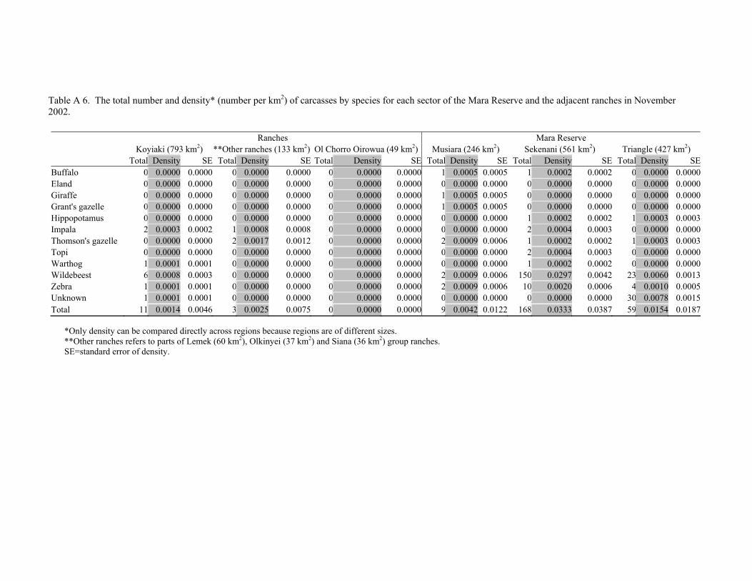
Table A 6. The total number and density* (number per km2) of carcasses by species for each sector of the Mara Reserve and the adjacent ranches in November 2002.

Ranches Mara Reserve Koyiaki (793 km2) **Other ranches (133 km2) Ol Chorro Oirowua (49 km2) Musiara (246 km2) Sekenani (561 km2) Triangle (427 km2)

Total Density SE Total Density SE Total Density SE Total Density SE Total Density SE Total Density SEBuffalo 0 0.0000 0.0000 0 0.0000 0.0000 0 0.0000 0.0000 1 0.0005 0.0005 1 0.0002 0.0002 0 0.0000 0.0000Eland 0 0.0000 0.0000 0 0.0000 0.0000 0 0.0000 0.0000 0 0.0000 0.0000 0 0.0000 0.0000 0 0.0000 0.0000Giraffe 0 0.0000 0.0000 0 0.0000 0.0000 0 0.0000 0.0000 1 0.0005 0.0005 0 0.0000 0.0000 0 0.0000 0.0000Grant's gazelle 0 0.0000 0.0000 0 0.0000 0.0000 0 0.0000 0.0000 1 0.0005 0.0005 0 0.0000 0.0000 0 0.0000 0.0000Hippopotamus 0 0.0000 0.0000 0 0.0000 0.0000 0 0.0000 0.0000 0 0.0000 0.0000 1 0.0002 0.0002 1 0.0003 0.0003Impala 2 0.0003 0.0002 1 0.0008 0.0008 0 0.0000 0.0000 0 0.0000 0.0000 2 0.0004 0.0003 0 0.0000 0.0000Thomson's gazelle 0 0.0000 0.0000 2 0.0017 0.0012 0 0.0000 0.0000 2 0.0009 0.0006 1 0.0002 0.0002 1 0.0003 0.0003Topi 0 0.0000 0.0000 0 0.0000 0.0000 0 0.0000 0.0000 0 0.0000 0.0000 2 0.0004 0.0003 0 0.0000 0.0000Warthog 1 0.0001 0.0001 0 0.0000 0.0000 0 0.0000 0.0000 0 0.0000 0.0000 1 0.0002 0.0002 0 0.0000 0.0000Wildebeest 6 0.0008 0.0003 0 0.0000 0.0000 0 0.0000 0.0000 2 0.0009 0.0006 150 0.0297 0.0042 23 0.0060 0.0013Zebra 1 0.0001 0.0001 0 0.0000 0.0000 0 0.0000 0.0000 2 0.0009 0.0006 10 0.0020 0.0006 4 0.0010 0.0005Unknown 1 0.0001 0.0001 0 0.0000 0.0000 0 0.0000 0.0000 0 0.0000 0.0000 0 0.0000 0.0000 30 0.0078 0.0015Total 11 0.0014 0.0046 3 0.0025 0.0075 0 0.0000 0.0000 9 0.0042 0.0122 168 0.0333 0.0387 59 0.0154 0.0187

*Only density can be compared directly across regions because regions are of different sizes. **Other ranches refers to parts of Lemek (60 km2), Olkinyei (37 km2) and Siana (36 km2) group ranches. SE=standard error of density.