performance and total pm emission factor evaluation of
TRANSCRIPT

University of New Orleans University of New Orleans
ScholarWorks@UNO ScholarWorks@UNO
University of New Orleans Theses and Dissertations Dissertations and Theses
5-22-2006
Performance and Total PM Emission Factor Evaluation of Performance and Total PM Emission Factor Evaluation of
Expendable Abrasives Expendable Abrasives
Kalpalatha Kambham University of New Orleans
Follow this and additional works at: https://scholarworks.uno.edu/td
Recommended Citation Recommended Citation Kambham, Kalpalatha, "Performance and Total PM Emission Factor Evaluation of Expendable Abrasives" (2006). University of New Orleans Theses and Dissertations. 385. https://scholarworks.uno.edu/td/385
This Dissertation is protected by copyright and/or related rights. It has been brought to you by ScholarWorks@UNO with permission from the rights-holder(s). You are free to use this Dissertation in any way that is permitted by the copyright and related rights legislation that applies to your use. For other uses you need to obtain permission from the rights-holder(s) directly, unless additional rights are indicated by a Creative Commons license in the record and/or on the work itself. This Dissertation has been accepted for inclusion in University of New Orleans Theses and Dissertations by an authorized administrator of ScholarWorks@UNO. For more information, please contact [email protected].

PERFORMANCE AND TOTAL PM EMISSION FACTOR EVALUATION OF
EXPENDABLE ABRASIVES
A Dissertation
Submitted to the Graduate Faculty of the University of New Orleans in partial fulfillment of the
requirements for the degree of
Doctor of Philosophy in
Engineering and Applied Science
by
Kalpalatha Kambham
B.S., S.V.University College of Engineering, 1999 M.S., University of New Orleans, 2002
May 2006

ii
ACKNOWLEDGEMENTS I would like to express my sincere gratitude to my advisor, Dr. Bhaskar Kura from the
Department of Civil and Environmental Engineering, whose advice, support, and encouragement
have provided me with an invaluable source of motivation over the last five years.
I am grateful to Dr. Donald E. Barbé, Dr. Gianna M. Cothren, Dr. William H. Busch, and Dr.
Matthew Tarr for serving on my Ph.D. Examining Committee and providing me with further
assistance. I am also grateful to Dr. Tumulesh Solanky from the Department of Mathematics for
his advice on statistical analysis.
I would like to thank my friends Sivaramakrishnan Sangameswaran, Xavier Silvadasan and
Babruvahan Hottangada, without whose help my research work would not have been successful.
I would especially like to thank my parents, whose love and great support was indispensable, and
who have provided me with lifetime motivation and inspiration. I would also like to thank my
sister and brother for their boundless love and encouragement. I would like to dedicate this work
to my family.
My greatest appreciation goes to my beloved husband Sunil Battepati, for his encouragement and
support over the last years.
iii
TABLE OF CONTENTS List of Tables .................................................................................................................................. v List of Figures ................................................................................................................................ vi Abstract ......................................................................................................................................... vii 1. Introduction................................................................................................................................. 1 2. Scope and Objectives.................................................................................................................. 3 3. Literature Review........................................................................................................................ 5
3.1. Dry Abrasive Blasting.......................................................................................................... 5 3.2. Pollutant Outputs and Their Effects on Health and Environment ....................................... 5
3.2.1. Air Emissions................................................................................................................ 5 3.2.2. Solid/ Hazardous Waste................................................................................................ 6
3.3. Important Parameters in Dry Abrasive Blasting.................................................................. 7 3.3.1. Abrasive Material.......................................................................................................... 7 3.3.2. Process Parameters and Equipment .............................................................................. 9 3.3.3. Initial Surface Contamination ..................................................................................... 12 3.3.4. Desired Surface Finish................................................................................................ 13 3.3.5. Waste Generation Potential......................................................................................... 14 3.3.6. Reusability .................................................................................................................. 14
3.4. Regulations ........................................................................................................................ 15 3.4.1. Federal Regulations .................................................................................................... 15 3.4.2. State Regulations and Guidelines ............................................................................... 19
3.5. Available Data for Emission Factors ................................................................................. 21 3.5.1. U.S. EPA Emission Factors ........................................................................................ 22 3.5.2. Emission Factors from State/ Environmental Agencies ............................................. 25
3.6. Available Data for Productivity and Consumption............................................................ 26 3.7. Previous Studies at UNO ................................................................................................... 28
4. Methodology............................................................................................................................. 29 4.1. Abrasive Materials ............................................................................................................. 29
4.1.1. Coal Slag..................................................................................................................... 29 4.1.2. Copper Slag................................................................................................................. 30 4.1.3. Specialty Sand............................................................................................................. 30
4.2. Equipment .......................................................................................................................... 31 4.2.1. Test Chamber .............................................................................................................. 32 4.2.2. Blasting Equipment..................................................................................................... 32 4.2.3. Test Plates ................................................................................................................... 34 4.2.4. Air Compressor........................................................................................................... 35 4.2.5. Exhaust Duct System .................................................................................................. 35 4.2.6. Stack Sampling System............................................................................................... 36 4.2.7. Particulate Collection System..................................................................................... 37
4.3. Experimental Parameters ................................................................................................... 38 4.3.1. Variable Parameters .................................................................................................... 38 4.3.2. Constant Parameters.................................................................................................... 38
4.4. Experimental Procedure..................................................................................................... 39 4.4.1. Abrasive Blasting........................................................................................................ 39 4.4.2. PM Sampling .............................................................................................................. 40

iv
4.5. Statistical Analysis............................................................................................................. 42 5. Results and Discussion ............................................................................................................. 45
5.1. Emission Factors................................................................................................................ 52 5.1.1. Emission Factors in kg/m2 .......................................................................................... 52 5.1.2. Emission Factors in kg/kg........................................................................................... 59
5.2. Productivity........................................................................................................................ 67 5.1.1. Variation of Productivity with Pressure...................................................................... 67 5.1.2. Variation of Productivity with Feed Rate ................................................................... 69 5.1.3. Variation of Productivity with Pressure and Feed Rate.............................................. 71
5.3. Consumption...................................................................................................................... 74 5.3.1. Variation of Consumption with Pressure.................................................................... 74 5.3.2. Variation of Consumption with Feed Rate ................................................................. 76 5.3.3. Variation of Consumption with Pressure and Feed Rate ............................................ 78
6. Conclusions and Recommendations ......................................................................................... 81 References..................................................................................................................................... 84 APPENDIX A: Field Observations and Stack Calculations......................................................... 89 APPENDIX B: Results of Statistical Analysis ............................................................................. 93 APPENDIX C: Material Data Safety Sheets .............................................................................. 103 APPENDIX D: Example for Calculation of Blasting Costs....................................................... 118 VITA........................................................................................................................................... 122

v
List of Tables
Table 1: NAAQS for PM10 and PM2.5........................................................................................ 16 Table 2: Summary of Test Data for Abrasive Blasting Operations .............................................. 23 Table 3: Particulate Emissions Factors for Abrasive Blasting...................................................... 25 Table 4: Available Emission Factors for PM................................................................................ 26 Table 5: Experimental Results for Coal Slag................................................................................ 46 Table 6: Mean and Standard Deviation (SD) of Experimental Results for Coal Slag.................. 47 Table 7: Experimental Results for Copper Slag ........................................................................... 48 Table 8: Mean and Standard Deviation (SD) of Experimental Results for Copper Slag ............. 49 Table 9: Experimental Results for Specialty Sand ....................................................................... 50 Table 10: Mean and Standard Deviation (SD) of Experimental Results for Specialty Sand ....... 51 Table 11: Coefficients for Emission Factors in (kg/m2) for Equation 2 ....................................... 59 Table 12: Coefficients for Emission Factors in (kg/kg) for Equation 3 ....................................... 65 Table 13: Coefficients for Productivity (m2/hr) for Equation 4.................................................... 73 Table 14: Coefficients for Consumption (kg/m2) for Equation 5 ................................................. 80

vi
List of Figures
Figure 1: Emissions Test Facility ................................................................................................. 31 Figure 2: Blast Pot ........................................................................................................................ 33 Figure 3: Exhaust Duct System..................................................................................................... 36 Figure 4: Two-Stage Particle Collection System.......................................................................... 38 Figure 5: Variation of Emission Factors (kg/m2) with Pressure at 3 Turns.................................. 52 Figure 6: Variation of Emission Factors (kg/m2) with Pressure at 4 Turns.................................. 53 Figure 7: Variation of Emission Factors (kg/m2) with Pressure at 5 Turns.................................. 54 Figure 8: Variation of Emission Factors (kg/m2) with Feed Rate at 80 PSI................................. 55 Figure 9: Variation of Emission Factors (kg/m2) with Feed Rate at 100 PSI............................... 56 Figure 10: Variation of Emission Factors (kg/m2) with Feed Rate at 120 PSI............................. 56 Figure 11: Coal Slag-Variation of Emission Factors (kg/m2) with Pressure and Feed Rate ........ 57 Figure 12: Copper Slag-Variation of Emission Factors (kg/m2) with Pressure and Feed Rate.... 58 Figure 13: Specialty Sand-Variation of Emission Factors (kg/m2) with Pressure and Feed Rate 58 Figure 14: Variation of Emission Factors (kg/kg) with Pressure at 3 turns.................................. 60 Figure 15: Variation of Emission Factors (kg/kg) with Pressure at 4 turns.................................. 61 Figure 16: Variation of Emission Factors (kg/kg) with Pressure at 5 turns.................................. 61 Figure 17: Variation of Emission Factors (kg/kg) with Feed Rate at 80 PSI ............................... 62 Figure 18: Variation of Emission Factors (kg/kg) with Feed Rate at 100 PSI ............................. 63 Figure 19: Variation of Emission Factors (kg/kg) with Feed Rate at 120 PSI ............................. 64 Figure 20: Coal Slag-Variation of Emission Factors (kg/kg) with Pressure and Feed Rate......... 65 Figure 21: Copper Slag-Variation of Emission Factors (kg/kg) with Pressure and Feed Rate .... 66 Figure 22: Specialty Sand-Variation of Emission Factors (kg/kg) with Pressure and Feed Rate 66 Figure 23: Variation of Productivity with Pressure at 3 Turns..................................................... 68 Figure 24: Variation of Productivity with Pressure at 4 Turns..................................................... 68 Figure 25: Variation of Productivity with Pressure at 5 Turns..................................................... 69 Figure 26: Variation of Productivity with Feed Rate at 80 PSI.................................................... 70 Figure 27: Variation of Productivity with Feed Rate at 100 PSI.................................................. 70 Figure 28: Variation of Productivity with Feed Rate at 120 PSI.................................................. 71 Figure 29: Coal Slag-Variation of Productivity with Pressure and Feed Rate ............................. 72 Figure 30: Copper Slag-Variation of Productivity with Pressure and Feed Rate ......................... 72 Figure 31: Specialty Sand-Variation of Productivity with Pressure and Feed Rate ..................... 73 Figure 32: Variation of Consumption with Pressure at 3 Turns ................................................... 74 Figure 33: Variation of Consumption with Pressure at 4 Turns ................................................... 75 Figure 34: Variation of Consumption with Pressure at 5 Turns ................................................... 76 Figure 35: Variation of Consumption with Feed Rate at 80 PSI .................................................. 77 Figure 36: Variation of Consumption with Feed Rate at 100 PSI ................................................ 77 Figure 37: Variation of Consumption with Feed Rate at 120 PSI ................................................ 78 Figure 38: Coal Slag - Variation of Consumption with Pressure and Feed Rate ......................... 79 Figure 39: Copper Slag - Variation of Consumption with Pressure and Feed Rate ..................... 79 Figure 40: Specialty Sand - Variation of Consumption with Pressure and Feed Rate ................. 80

vii
Abstract
Dry abrasive blasting is one of the most widely used methods of surface preparation. Air
emissions from this process include particulate matter (PM) and metals. Spent abrasive generated
from this process may be hazardous in nature. With increasing concern on health effects due to
silica emissions from sand, use of alternative materials is suggested by health and regulatory
agencies.
The objective of this research was to evaluate performance of expendable abrasives and
determine PM emission factors. Dry abrasive blasting was performed in an enclosed chamber
and total PM samples were collected. Three commonly used expendable abrasives, coal slag,
copper slag and specialty sand, were used to evaluate cleaner alternatives. Blast pressure and
abrasive feed rate, two important process conditions were varied to study their effect on
performance of an abrasive. Productivity, consumption and emission factors (performance
parameters) were calculated and their variation with pressure and feed rate was evaluated. Two
dimensional and three dimensional predicted models were developed to estimate the
performance at intermediate blast pressure and feed rate conditions. Performance of the three
abrasives was compared with respect to emission potential, productivity and consumption.
Emission factors developed in this research will help in accurate estimation of total PM
emissions and to select cleaner abrasives and optimum process conditions that will results in
minimum emissions and reduced health risk.

viii
The productivity and consumption models will help is estimating life cycle costs including
material cost, equipment cost, energy cost, labor costs, waste disposal cost, and compliance
costs. Consumption models will also help in determining the quantity of spent abrasive
generated, identify abrasives with lower material consumption, and identify process conditions
that generate minimum spent abrasives. In addition, these models will help industries in making
environmentally preferable purchasing (EPP), which results in pollution prevention and cost
reduction.

1
1. Introduction
Dry abrasive blasting is one of the widely used methods of surface preparation for steel
or metal surfaces. This process is used to create a rough profile and to remove contaminants such
as rust or old coating before applying a new coating to ensure proper bonding between the
surface and coating. Several industries such as aerospace, automobile, bridge construction, metal
finishing, shipbuilding and ship repair use dry abrasive blasting for preparation and maintenance
of steel or other metal surfaces (U.S. ACE 1995, U.S. EPA 1997a). In this process, abrasive
materials are propelled at high velocities with the aid of compressed air. The energy transfer
between the abrasive grains and base plate results in removal of contaminants and creation of
rough profile (U.S. ACE 1995).
Some of the commonly used abrasives are coal slag, copper slag, garnet, silica sand,
specular hematite (barshot), steel grit, steel shot, aluminum oxide, silicon carbide etc. (U.S. EPA,
1997a). Dry abrasive blasting process results in air emissions (particulate matter and metals) and
spent blast media which may be harmful to human health and environment (U.S. EPA 1997b).
Silica sand has been widely used as an abrasive material due to its low cost and abundant
occurrence in nature. However, silica dust emissions from abrasive blasting with silica sand have
been of great concern due to adverse health effects on workers upon exposure to these emissions.
Thus, use of alternative materials to silica sand is suggested by several health organizations and
environmental agencies (NIOSH 1998, Abrasive Blasting, 1995) to protect worker health as well
as the environment.
In addition, owing to the environmental impacts of the process and waste management
challenges faced for safe disposal of the wastes, United States Environmental Protection Agency
(US EPA) encourages industries, businesses, and institutions to make environmentally preferable

2
purchasing (EPP), which means considering the environmental impacts (air and water pollution,
toxic wastes), energy-efficient technologies and material performance prior to purchasing
materials. This will result in resource conservation, waste minimization, minimization of energy
consumption, and extension of landfill capacity. In addition, costs incurred due to material
purchase, energy consumption, waste management and disposal can be reduced by EPP (U.S.
EPA 1994, U.S. EPA 2001).
In order to address and achieve the above mentioned objectives, namely, protect worker
health, environment and make EPP, it is important to evaluate waste generation potential (air
emissions and spent abrasive) and performance of alternate abrasive materials as well as
understand the effect of various parameters that affect performance and waste generation
potential. Performance of abrasive in dry abrasive blasting depends on properties of abrasive
material (size, shape, hardness, and chemical composition), blast pressure, abrasive feed rate,
nozzle size, base plate (substrate), surface contamination, quality of desired finish and others
(U.S. ACE 1995). While some abrasives can be reused in abrasive blasting, others can not be
reused due to their properties such as hardness and dust generation rate. These materials are
called expendable or non-reusable abrasives. The goal of this research was to evaluate
performance of expendable abrasives to identify cleaner alternatives and process conditions that
will result in pollution prevention and cost reduction.

3
2. Scope and Objectives
Existing literature provides limited data on performance, process conditions and test
procedures adopted for evaluating the performance of alternative materials for dry abrasive
blasting. This research was focused on evaluating performance of three of the most commonly
used expendable (single use) abrasive materials, namely coal slag, copper slag and specialty
sand, on painted mild steel surfaces.
The primary objectives of this research were:
Objective 1: The first objective of this research was to determine emission factors for
total particulate matter (TPM). Emission factors help in quantifying the
emissions released from a process and these are important input
parameters in developing emission inventories.
Objective 2: The second objective of this research was to determine productivity. Productivity
(or cleaning rate) determines how fast the surface can be cleaned (area cleaned
per unit time). The higher the productivity, the faster the cleaning rate and less
consumption of energy. Higher productivity also results in reduced labor and
energy costs.
Objective 3: The third objective of this research was to determine consumption. Consumption
is the amount of material used to clean a unit area. Lower consumption results in
better conservation of resources, reduced amounts of wastes generated and
efficient use of landfills for waste disposal. In addition, lower consumption results
in reduced material costs, waste management and disposal costs.
Objective 4: The fourth objective of this research was to identify optimum process
conditions (blast pressure and abrasive feed rate) to minimize total PM
4
emissions and abrasive consumption, and maximize productivity. Since
the performance of an abrasive depends of process conditions, it is
important to study the variation of performance with process conditions to
achieve maximum efficiency through process optimization.
Objective 5: The fifth objective of this study was to develop predictive mathematical
models to estimate total PM emission factors, productivity and
consumption at intermediate operating conditions for a specific abrasive
material. These models will help industries and regulatory agencies in
determining accurate TPM emissions and assist in life cycle cost and
assessment methodologies with more accurate data on productivity and
consumption.
Objective 6: The sixth objective of this research was to compare the three abrasives
based on emission factors, productivity and consumption.

5
3. Literature Review
3.1. Dry Abrasive Blasting Surface preparation methods are used to remove impurities such as rust, corrosion, and
old coatings from a substrate and create a rough profile (or anchor pattern) that will help better
adhesion of new coating as well as improve the performance of new coating. Some of the most
commonly used methods are dry abrasive blasting, wet abrasive blasting, hydro blasting (water
blasting), chemical stripping, and vacuum blasting. Dry abrasive blasting is one of most effective
and widely used methods of surface preparation. In this method, an abrasive material is mixed
with compressed air and this mixture is projected onto the surface. The pressurized air
(compressed air) imparts high velocities to the abrasive particles. The mass of abrasive particles
and high velocity imparted by the compressed air create kinetic energy, which is given by ½
mV2, where m is the mass and V is the velocity of the abrasive material. The energy transfer
between the abrasive material and the surface is responsible for removing the contaminants and
creating the required profile (U.S. ACE 1995, U.S. EPA 1997a). The equipment used in this
process is discussed in the Methodology Section.
3.2. Pollutant Outputs and Their Effects on Health and Environment
3.2.1. Air Emissions
The abrasive particles, when bombarding the surface at high velocities, remove the
contaminants and breakdown into smaller particles. This process releases particulate matter (PM)
that includes blast material as well as contaminants removed (U.S. ACE 1995, U.S. EPA 1997a,
NIOSH 1998). These particles vary in size and may contain metals such as arsenic, cadmium,
chromium (trivalent and hexavalent), lead, manganese, nickel, and titanium (NIOSH 1998,
6
NSRP 1999, Vallyathan et al 1999, Conroy et al 1996, MacKay et al 1980). Particulate
emissions are of great concern due to the health effects, visibility impairment, ecosystem
imbalance and aesthetic damage. Fine particulates can be carried over long distances and settle
on ground or water. This may make lakes and streams acidic, change nutrient balance is coastal
waters, and deplete nutrients in soil. Inhalation of particulate matter causes respiratory problems,
asthma, chronic bronchitis, and decreased lung function (U.S. EPA, Dockery et al 1993,
Oberdorster 1995, Pope et al 1995). Recent studies (Wilson et al 1985, Daigle et al 2003, U.S.
EPA, 2004a, U.S. EPA, 2004b, Voutilainen et al 2004) on health effects of PM show that fine
(PM less than 2.5 μm in diameter) and ultrafine particles (PM less than 0.1 μm in diameter) have
significantly greater effects on respiratory systems and lung functions because finer particles are
absorbed into the respiratory system and lungs as compared with coarser particles. Moreover,
ultrafine particles deposited in lungs release toxic compounds (associated with PM) faster than
fine and coarse particles. The emissions may be toxic due to heavy metals present in airborne
particulates and exposure to these emissions may cause adverse health effects (specific) (Hubbs
et al 2001, Vallyathan et al 1999, Conroy et al 1996, MacKay et al 1980, NIOSH 2001). Most
importantly, exposure to silica dust emitted from sandblasting, abrasive blasting with silica sand,
causes silicosis (NIOSH 1974, Lipton and Herring 1996, Rappaport et al 2003).
3.2.2. Solid/ Hazardous Waste
While lighter particles get airborne, heavier particles fall off and this waste (spent
abrasive) contains both abrasive materials and contaminants removed such as rust or paint chips.
The waste may be toxic if the abrasive material or surface contamination contains heavy metals
such as arsenic, lead, chromium, and others (NFESC 1996, Townsend 1997, NAVFAC 1998,
Angie and Wayne 1999). In case of removal of coatings that contain lead or antifouling agents,

7
the waste generated may be hazardous (U.S. EPA 1997b). The spent abrasive media may be
recycled or reused for blasting operations or other purposes if the material is clean enough and
meets the regulatory requirements for recycling and reusing options. If the spent abrasive cannot
be recycled or reused, it must be disposed of as a solid or hazardous waste in landfills depending
on the toxic characteristics of the waste, which are determined by Toxicity Characteristic
Leaching Procedure (TCLP) tests (Townsend 1997, NFESC 1996, Angie and Wayne 1999).
3.3. Important Parameters in Dry Abrasive Blasting
3.3.1. Abrasive Material
Proper selection of abrasive material is essential to achieve maximum efficiency in dry
abrasive blasting. Some of the important parameters are: abrasive cost, abrasive type,
characteristics of the material, surface to be cleaned, contaminants to removed, level of
contamination, surface finish desired (cleanliness and profile), waste generation potential,
consumption rate, reusability, and others. Significance of some of these parameters is discussed
in this section.
3.3.1.1. Abrasive type
Abrasive materials are generally categorized into slag abrasives, metallic abrasives,
natural abrasives, and synthetic abrasives. The slag abrasives are by-products from smelting and
combustion processes. Coal slag, copper slag, and nickel slag are some of the most widely used
slag abrasives. These abrasives have high breakdown rates and thus, slag abrasives are generally
not reused. Due to their dark color, these materials may leave dark residue on the blasted surface.
Metallic abrasives such as steel grit, steel shot, and cast iron are manufactured abrasives. These
abrasives are hard and can be reused many times. Natural abrasives include silicates (sand,
garnet, olivine), hematite and others. The abrasive properties of these naturally occurring

8
materials are enhanced by washing and grading the material. Synthetic abrasives include
aluminum oxides, aluminum silicates, calcium silicate, crushed glass, glass beads, and others.
The performance of these abrasives depends on the surface type and contamination to be
removed (U.S. EPA 1997a, Paddison 2000, Hansink 2000)
3.3.1.2. Abrasive particle size
Particle size of abrasive material is an important factor in selection of abrasives. The size
of abrasive particles varies widely between 0.06 to 2 mm. Too fine or coarse particles may not be
effective in removing contamination and creating the desired profile. While larger particles cut
deep into the surface and create deep surface profile, smaller particles create shallow profiles. In
addition, if the particle size is too high, a smaller number of particles impact the surface which
increases material consumption and decreases productivity as compared to smaller particles that
result in greater number of impacts per unit surface area. Since abrasive particles breakdown into
smaller particles upon striking the surface, too fine abrasive materials may release very fine PM,
which is of great concern due to associated health effects. While a mixed size of particles may
result in better performance, particle size is important when selecting reusable or expendable
(single use) abrasives. In case of reusable abrasives, it is important to select an abrasive particle
size which results in efficient size of reusable abrasive material after breaking down into smaller
particles (U.S. ACE 1995, Paddison 2000, Hansink 2000).
3.3.1.3. Abrasive particle shape
The shape of abrasive particles is important in determining the surface profile required.
While angular particles cut the surface, round particles peen the surface. Thus, round particles
such as steel shot and glass beads are effective for removing mill scale and angular particles such
9
as steel grit, slags, and other metallic grits are effective for creating a rough profile (U.S. ACE
1995, Hansink 2000).
3.3.1.4. Hardness
Hardness of an abrasive material indicates its resistance to abrasion by other materials.
Hardness of abrasives is measured on Mohs scale of hardness. Metallic and slag abrasives have
higher hardness (6 – 8 Mohs) and cut deeper and faster than soft or brittle abrasives such as
organic or plastic abrasive media (2 – 4 Mohs) reducing their cleaning efficiency (U.S. ACE
1995, Paddison 2000, Hansink 2000).
3.3.1.5. Specific gravity
As mentioned earlier in Section 3.1, the kinetic energy of the abrasive particles is given
by ½ mV2. Mass of abrasive material, m, is proportional to specific gravity (SG) of the abrasive
particles. Abrasives with higher SG are more efficient and clean faster, which increase
productivity (Paddison 2000, Hansink 2000).
3.3.1.6. Density
Density of abrasive material is important in selecting the size of blast pot and storing the
abrasive material. Since lower density abrasives occupy more volume for the same mass, bigger
blast pot and greater storage area are needed as compared to abrasives with higher density, which
occupy less volume and need smaller blast pots and storage areas (Hansink 2000).
3.3.2. Process Parameters and Equipment
3.3.2.1. Blast pressure
Blast pressure determines the velocity of abrasive particles and hence kinetic energy
acquired by the particles. Thus, increase in pressure increases the kinetic energy of particles and
hence the impact on a surface. This results in higher productivity. However, at very high

10
pressures, the particles may suffer more damage due to collision of these particles with
rebounding particles before striking the surface and reduce productivity, increase consumption,
and results in higher emissions. In addition, blasters may not be able to handle these high
pressures and must be provided with additional protection. At very low pressures, the velocity of
particles is less and the particles may not strike the surface with sufficient impact to remove
contaminants and create required profile. This will result in decreased productivity and increased
consumption since more material is required to clean a unit surface area. Very low pressures may
also result in fewer emissions due to less breakdown rate at lower velocities (Clemco Industries
1989, Hansink 1995, Holt and Austin 2001, Paddison 2000, Seavey 1985). Thus, it is important
to select an optimum pressure that results in high productivity, low consumption, and low
emissions while providing a safe working environment for workers.
3.3.2.2. Abrasive feed rate
Feed rate determines the mass flow rate of abrasive. Very low feed rates may result in
uneven distribution of particles and decrease productivity while consuming more material. As
the feed rate is increased, more abrasive is released which increases productivity and more
number of abrasive particles breakdown, causing increase in emissions. However, at very high
feed rates, the same effect may not be observed because abrasive particles collide with
rebounding particles and decrease productivity while consuming more material. An increase in
emissions may occur at very high feed rates due to more number of particles participating in the
abrading action (Clemco Industries 1989, Hansink 1995, Paddison 2000). Thus, it is important to
regulate the flow of material to achieve maximum efficiency from a given mass of abrasive
while reducing emissions.
11
3.3.2.3. Nozzle size
Nozzle sizes used in abrasive blasting typically range from 1/8 inch to 1/2 inch orifice
diameter. While larger nozzles may increase productivity by increasing the number of impacts
per unit time by allowing more abrasive to flow through the nozzle, smaller nozzles may also
increase productivity due to increase in blast pressure. However, for the same volume of air,
larger nozzles require high capacity compressors to provide required blast pressure to achieve
higher productivity (U.S. ACE 1995, Gorripati 2000). Thus, selecting the proper size of nozzle is
important in maintaining required blast pressure and determining the capacity of air compressor.
3.3.2.4. Nozzle type
Venturi and straight-bore nozzles are two types of nozzles used in abrasive blasting
process. Venturi nozzles converge to specified orifice diameter at the center of the nozzle and
then diverge. This enables an increase of exit velocity of abrasive particles and thus increases the
productivity. Straight-bore nozzles have uniform diameter throughout the length of the nozzle.
Thus, venturi nozzles provide higher cleaning rate as compared to straight-bore nozzles. Blast
nozzles are available in various lengths, diameters and lining materials. The life of a nozzle
depends on the lining materials. Nozzles lined with tungsten or boron carbides have longer life
than the nozzles lined with ceramic or cast iron (U.S. ACE 1995, Gorripati 2000).
3.3.2.5. Angle of deflection
Angle of deflection or angle of attack is the angle of the nozzle with respect to the work
piece or surface being blasted. This parameter depends on the surface contamination being
removed and varies between 45 to 90 degrees. While for removing rust and mill scale, angle of
deflection may vary from 80 to 90 degrees whereas for removing old coatings, it may vary from
12
45 to 60 degrees (U.S. ACE 1995). In some cases, nozzles held at an angle of greater or lesser
than 90 degrees may scour the surface (Gorripati 2000).
3.3.2.6. Stand-off distance
Stand-off distance is the distance between the nozzle and the work piece or surface. This
may vary from 6 to 24 inches (15 to 60 cm). The closer the distance, the smaller the blast pattern.
In case of removing mill scale or heavy levels of contamination, a lesser stand-off distance
creates greater impact and increases cleaning power. However, this may reduce productivity due
to decreased blast pattern. For removing smaller levels of contamination, this distance may be
increased to increase the blast pattern and thus achieve higher productivity. Hence, optimum
stand-off distance is important since it affects the blast pattern, productivity and impact of the
abrasive material (U.S. ACE 1995, Gorripati 2000).
3.3.2.7. Dwell time
Dwell time is the amount of time spent cleaning a particular area on the surface to
achieve required cleanliness and profile. For removing lightly adhered contaminants or smaller
levels of contamination, shorter periods will achieve the desired finish. When removing tightly
adhered contaminants or greater levels of contamination, it may take longer time to clean the
surface. In addition, if the nozzle is held close to the surface, lesser dwell time is required as
compared to when nozzle is held far from the surface. Thus, angle of deflection and stand-off
distance also affect dwell time (Gorripati 2000, Technology Publishing Company 1999).
3.3.3. Initial Surface Contamination
Performance of an abrasive also depends on the type of contamination to be removed. For
heavy levels of contamination, it may take longer time and consume more material to clean a
unit surface area. This will decrease productivity, increase consumption and waste quantities

13
generated. The type of contamination being removed such as rust, mill scale or paint determines
the toxic characteristics of the emissions and spent abrasive generated. In the case of removing
lead-based paints, resulting wastes may be toxic due to the presence of lead.
In addition, depending on the properties of abrasive such as particle size, shape and
hardness, a particular abrasive may be more effective in removing rust while another abrasive
may be more effective in removing paint. Thus, it is important to determine level and
composition of the contaminants being removed to achieve maximum efficiency from an
abrasive material and the dry abrasive blasting process.
3.3.4. Desired Surface Finish
Proper adhesion of new coating is important to its life and effectiveness. Thus, the
surface must be free of underlying dust and contamination. In addition, surface roughness or
profile is important for the new coating to adhere to the surface since it provides more surface
area for adhesion. For commercial steel structures, the Society of Protective Coatings provides
surface preparation standards in terms of quality of the finish. For example, SP-5 refers to a
white metal blasting, which involves removal of all visible rust, mill scale, paint and
contaminants, leaving the metal uniformly white or gray in appearance. SP-6 refers to a
commercial blast cleaning. According to this standard, all oil, grease, dirt, rust scale, old paint
and foreign matter must be completely removed from the surface except for slight shadows,
streaks or discolorations caused by rust stain, mill scale oxides, or slight, tight resides of paint or
coating that remain. SP-10 refers to brush-off blast finish. This standard requires removal of all
oil, grease, dirt, mill scale, rust, corrosion products, paint, or other foreign matter, except for very
light shadows, very slight streaks or slight discolorations caused by rust stain, mill scale oxides,
or slight residues of paint or coating. At least 95% of each square inch of surface area shall be

14
free of all visible residues (SSPC). The higher the quality of surface finish, the higher abrasive
consumption will be, air emissions, quantity of spent abrasive, and the lower productivity will be
since more material and time are consumed to clean a unit surface area. Thus, desired surface
finish or degree of cleaning is an important factor that must be considered while selecting an
abrasive material, process conditions and evaluating performance of abrasive materials.
3.3.5. Waste Generation Potential
Waste generation potential of an abrasive is important to evaluate health, safety and
environmental impact of the material as well as environmental compliance and waste disposal
costs in dry abrasive blasting. This depends on a number of factors including breakdown rate,
dust generation rate, and chemical composition. Abrasives with smaller particle size and brittle
properties generate more dust since they breakdown easily into very fine particles. In addition,
composition of the abrasive material such as metals, free silica content and other toxic chemicals
is important to assess the toxicity of both air emissions and spent abrasives. With increasing
concern on health effects due to silica emissions, abrasives with less free silica content (<1%)
must be used to protect worker health. Abrasive materials with less potential for waste
generation and decreased health risk due to exposure to toxic emissions, reduce the quantities
and concentrations of hazardous waste generated. Industries can reduce the costs incurred due to
environmental compliance and waste disposal (U.S. ACE 1995, NIOSH 1998, Appleman et al.
1998).
3.3.6. Reusability
Based on the reusability of abrasives, they can be categorized into reusable and non-
reusable or expendable abrasives. Abrasive properties such as particle size, hardness and
breakdown rate determine reusability of an abrasive. If the particle size of abrasive material is
15
too low or if the breakdown rate abrasive is too high, the spent abrasive generated may be too
fine to create the desired surface finish. And abrasives with high breakdown rates generate
significant amounts of dust, decrease productivity and increase abrasive consumption. Slag
abrasives such as coal slag and copper slag generate high dust and breakdown easily. Thus, the
materials are not reused. Harder abrasives such as steel grit and garnet may be reused for a
number of times based on their particle size and breakdown rate (U.S. ACE 1995, Paddison
2000, Hansink 2000). While non-reusable abrasives are cheaper than reusable abrasives, overall
costs incurred due to reuse of abrasives and cost of recycling the spent abrasive for reuse must be
considered while selecting an abrasive.
3.4. Regulations
3.4.1. Federal Regulations
3.4.1.1. Clean Air Act (CAA)
The Clean Air Act and the Clean Air Act Amendments (CAAA) of 1990 are intended to
protect and enhance the nation’s air resources, promote public health, and protect the
environment. Ambient air quality is regulated by the National Ambient Air Quality Standards
(NAAQS), established for six criteria pollutants: carbon monoxide, lead, nitrogen dioxide,
ozone, PM, and sulfur dioxide (U.S. EPA 2004). Of the six criteria pollutants, particulates and
lead (in case of lead-based paints) can be generated during dry abrasive blasting. Particulate
matter (PM) is a mixture of solid and liquid particles suspended in air. PM may be directly
emitted from industrial processes and motor vehicles. PM may also be formed in atmosphere due
to chemical reaction of pollutants from these sources.
16
The size and composition of PM varies widely and particulates less than 10 micrometers
in diameter (PM10) cause serious health effects. Larger particles cause irritation to eyes, nose,
and throat (U.S. EPA, 2003). Exposure to PM has been associated with various health effects
including asthma, chronic bronchitis, premature death, decreased lung function, and severe
respiratory problems (U.S. EPA 2003, Pope et al. 1995, Atkinson et al. 2001, Schwartz 2004,
Dockery et al. 1993). Thus, in order to regulate these PM concentrations, NAAQS established
new standards for PM10, PM2.5. Two types of standards, primary standards and secondary
standards are developed to protect public health, and to prevent environmental damage
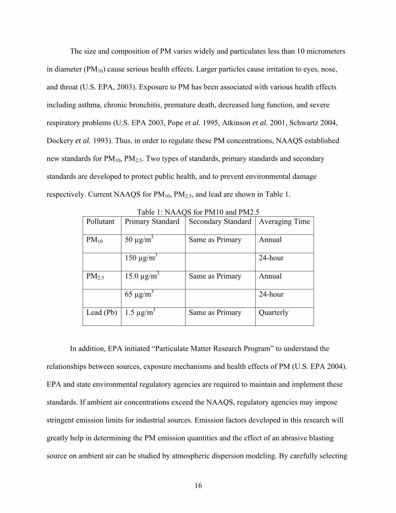
respectively. Current NAAQS for PM10, PM2.5, and lead are shown in Table 1.
Table 1: NAAQS for PM10 and PM2.5 Pollutant Primary Standard Secondary Standard Averaging Time
PM10 50 µg/m3 Same as Primary Annual
150 µg/m3 24-hour
PM2.5 15.0 µg/m3 Same as Primary Annual
65 µg/m3 24-hour
Lead (Pb) 1.5 µg/m3 Same as Primary Quarterly
In addition, EPA initiated “Particulate Matter Research Program” to understand the
relationships between sources, exposure mechanisms and health effects of PM (U.S. EPA 2004).
EPA and state environmental regulatory agencies are required to maintain and implement these
standards. If ambient air concentrations exceed the NAAQS, regulatory agencies may impose
stringent emission limits for industrial sources. Emission factors developed in this research will
greatly help in determining the PM emission quantities and the effect of an abrasive blasting
source on ambient air can be studied by atmospheric dispersion modeling. By carefully selecting

17
an abrasive and process conditions, PM emissions can be reduced thereby attaining the emission
limits and NAAQS.
3.4.1.2. Resource Conservation and Recovery Act (RCRA)
Resource Conservation and Recovery Act regulates the waste generated from industrial
processes. Based on the characteristics of the waste, it is categorized as solid waste or hazardous
waste. Removal of coating may result in hazardous waste based on composition of the coating.
In case of hazardous waste, waste must be properly contained and disposed of to comply with the
generator, transporter, treatment, storage, and disposal (TSD) regulations. Facilities that generate
at least 100 kilograms of hazardous waste per month must comply with the hazardous waste
generator requirements according to 40 CFR Part 262 (PCRC, U.S. EPA, 1997b). Some of
sources of hazardous waste in dry abrasive blasting are toxic metals and blast media
contaminated with paint chips. Based on the consumption of abrasive materials, industries will
be able to estimate the quantities of spent abrasives and hazard wastes generated. With proper
selection of materials and process conditions, waste generation and costs incurred due to waste
management can be minimized.
3.4.1.3. Clean Water Act (CWA)
Clean Water Act regulates discharges of wastewater streams containing heavy metals,
toxic organics, and conventional pollutants. If the wastewater is discharged into rivers, lakes or
oceans, the facilities must comply with effluent limits according to National Pollutant Discharge
Elimination System (NPDES). Facilities that discharge wastewater streams into Publicly Owned
Treatment Works (POTW) must meet the effluent limits in their POTW agreements. Blast media
and residue from coating removal may contaminate waster streams or during clean up operations.
Some of the regulated pollutants such as lead, cadmium, zinc, total suspended particles may be
18
present in the wastewater generated from dry abrasive blasting. Facilities must periodically
monitor the wastewater to demonstrate compliance with the regulations. In case of exceeding the
effluent limits, facilities must treat the wastewater prior to final discharge (PCRC, Shipbuilding
Sector Notebook). Material substitution and process optimization will help in minimizing both
quantities and characteristics of wastewater generated and storm water contamination during
abrasive blasting.
3.4.1.3. Occupational Safety and Health Administration (OSHA)
In order to protect worker health from exposure to PM, silica dust, lead and other toxic
emissions, the Occupational Safety and Health Administration regulates health hazards due to
abrasive blasting. Abrasives with higher free silica content generate silica dust, which is
associated with acute silicosis, bronchitis, and lung cancer. OSHA enforces permissible exposure
limits (PEL) to reduce exposure of workers to respirable silica emissions. OSHA also suggests
using abrasives with less free silica contents. Other health hazards regulated by OSHA include
metal emissions, noise, and mechanical hazards during abrasive blasting. Abrasive blasting at
very high pressures may cause severe damage to workers limbs. Proper personal protective
equipment, engineering controls, worker training, and periodic medical examinations must be
employed to comply with the OSHA regulations (PCRS, NIOSH 1998). Emission potential of an
abrasive material can be determined by emission factors. Selecting a material with less emission
potential will reduce the emissions as well as exposure of workers to hazardous emissions. In
addition, selecting process condition to achieve maximum productivity will reduce the exposure
time and health risk associated with longer exposure time.
19
3.4.2. State Regulations and Guidelines
Due to significant hazards from silica-based abrasives and enormous amounts of dust
generated during abrasive blasting, many state agencies restrict the use of silica sand for outdoor
blasting and suggest using alternative materials to reduce silica emissions and their health effects
on workers and public. Regulations and guidelines by some of the state environmental agencies
are discussed in this section.
3.4.2.1. Bay Area Air Quality Management District (BAAQMD)
BAAQMD protects public health environment in San Francisco Bay region. BAAQMD
provides permit requirements, and performance standards for facilities that carry out abrasive
blasting operations (BAAQMD 1990, BAAQMD 1998). Abrasive materials used for unconfined
blasting operations must comply with particle size standards. According to these standards,
before blasting “Before blasting, the abrasive shall not contain more than 1% by weight material
passing a #70 U.S. Standard sieve when tested in accordance with “Method of Test for Abrasive
Media Evaluation,” Test Method No. California 371-A. Certified abrasives re-used for dry
unconfined blasting must conform with Section 12-4-305.1”. In order to control size of PM
emissions after blasting, “the abrasive shall not contain more than 1.8% by weight material five
micron or smaller when tested in accordance with “Method of Test for Abrasive Media
Evaluation”, Test Method No. California 371-A. Certified abrasives re-used for dry unconfined
blasting are exempt from Section 12-4-305.2”. All abrasive materials used for unconfined
blasting must be certified by California Air Resources Board (CARB). Confined blasting shall be
used for all abrasive blasting operations except when (a) using steel grit, steel shot, iron grit or
iron shot, (b) When the structure or item being blasting exceeds 8 feet in height, 8 feet in width,
or 10 feet in length, and (c) When the structure is at its permanent location.

20
3.4.2.2. Louisiana Department of Environmental Quality (LDEQ)
LDEQ regulates environmental quality of Louisiana State to protect the environment,
public health, and safety. Steel fabrication, shipbuilding, metal cleaning and any activity that
uses abrasives blasting must comply with regulations specified in LAC 33:III.1305.3 (LDEQ
1998). Some of the applicable regulations are discussed in this section. In case of outdoor
blasting, shrouds must be used at all the times during blasting to confine air emissions from
escaping into atmosphere. These shrouds (a) must be placed close to blast area to prevent
dispersion of emissions in larger areas, (b) must have overlapping seams to prevent leakage of
PM emissions, and (c) must repair tears greater than one foot in length before blasting is carried
out. Industries must use abrasives that contain less than 1% (by mass) of fines that would pass
through a No.80 sieve. Abrasive with less dust generation rates must be used. Materials derived
from hazardous, toxic, medical or municipal wastes are prohibited from use as abrasive
materials. In case of indoor blasting, the blast cabinets must be equipped with exhaust systems
and emission control equipment.
Industries must maintain a daily record of actual operating times and monthly records of
abrasive material usage with percentage mass of fines as specified by the manufacturer. During
blasting, precautions must be taken to prevent PM from becoming airborne. To minimize
hazardous waste generation, personnel must maintain optimum blast pressure levels, minimize
contamination of abrasive materials with hazardous wastes or lead paints, and remove spent
abrasives prior to working with surface that contain lead-based coatings.
3.4.2.3. Texas Natural Resource Conservation Commission (TNRCC) TNRCC’s Air Permits Division provides permit application information and applicable
regulations for facilities that perform dry abrasive blasting (TNRCC 2001). Facilities must
21
submit information on type abrasive blasting, abrasive materials and quantities used, size of blast
cabinet (in case of enclosed blasting), control equipment data, exhaust system data and methods
of disposal of wastes generated in order to obtain an operating permit (TNRCC 1993).
Facilities must estimate hourly and annual TSP and PM10 emissions using emission
factors specified by TNRCC. In addition, off-property concentrations of all chemicals must be
estimated. The off-property concentrations of PM cannot exceed 400 μg/m3 for any one-hour
period and cannot exceed 200 μg/m3 for any three-hour period. In addition, the facilities must
comply with NAAQS for PM10, PM2.5, and lead emissions.
3.5. Available Data for Emission Factors
Emission inventories are important tools for air quality management. These are used to
determine applicability of permitting programs, identify major sources of pollutants, and develop
emission control technologies. Emission factors (EF) are key input parameters for developing
emission inventories. Since 1972, U.S. EPA has been compiling and publishing emission factors
for various pollutants from a variety of stationary point and area sources in AP-42 documents
(U.S. EPA 1997c). An emission factor is defined as the quantity of pollutant released to the
atmosphere from a source in relation to an activity. Generally, emission factors are expressed in
terms of weight of pollutant emitted per unit weight, duration, volume or distance of the activity
that emits the pollutant. Usually, emission quantities are estimated using Equation 1 given
below:
⎥⎦
⎤⎢⎣
⎡⎟⎠⎞
⎜⎝⎛−=100
1** EREFAE (1)
where: E = emissions, A = activity rate, EF = uncontrolled emission factor, and ER = overall
emission reduction efficiency, %.

22
Emission factors can be developed using mass-balance approach, emissions monitoring,
engineering calculations, or a combination of these methods. AP-42 documents provide emission
factor ratings to indicate the robustness, or appropriateness of emission factors based on source
operation, sampling procedures, sampling and process data, analysis and calculations. These
ratings are given from A through E.
A = Excellent.
B = Above average.
C = Average.
D = Below average.
E = Poor.
Since emission factors represent average emission rate for an entire process or source
category, actual emissions may vary widely from one source to another.
3.5.1. U.S. EPA Emission Factors
Section 13.2.6, Emission Factor Documentation for AP-42, provides emission factor data
applicable for abrasive blasting processes (U.S. EPA 1997a). Emissions factors for TPM, PM10
PM2.5, derived from various studies conducted on sand and garnet are compiled in this document.
The test conditions and data quality ratings of these studies are shown in Table 2. The average
emission factors provided U.S. EPA, from these studies are shown in Table 3. These EFs are
given a rating of E, which means a poor quality. Since these EFs are based on wind velocity,
emissions from enclosed blasting operations may vary significantly from these values. In
addition, emission potential depends on abrasive material used, surface contamination being
removed, method of abrasive blasting, and other factors discussed in Section 3.3. Hence,
estimating emissions from this data may not represent actual emissions.
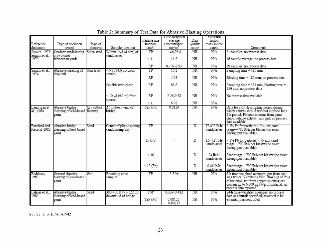
23
Table 2: Summary of Test Data for Abrasive Blasting Operations
Source: U.S. EPA, AP-42

24
(Table 2 continued..)
TP = total particulate matter. RP = respirable particulate matter (# 3.5 µmA) as determined using a 10-mm nylon cyclone followed by a 37-mm filter cassette. Source: U.S. EPA, AP-42

25
Table 3: Particulate Emissions Factors for Abrasive Blasting
Source: U.S. EPA, AP-42
3.5.2. Emission Factors from State/ Environmental Agencies
Available emission factors from environmental agencies from various states (TNRCC,
BAAQMD, SCAQMD, SDAPCD) are shown in Table 4. National Shipbuilding Research
Program developed emission factors for coal slag, copper slag, garnet, hematite, and sand at blast
pressures of 80 and 122 PSI for PM1, PM2.5, PM4, and PM10. The disadvantages of available
data on emission factors are some of the data are very general and do not provide process
condition information. While NSRP provided more information on process conditions, the data is
not continuous. Thus emissions cannot be estimated at intermediate operating conditions.
Moreover, these were based on mass-balance methods and may not represent true quantities of
emissions.

26
Table 4: Available Emission Factors for PM
Agency Abrasive Material PM Size EF (lbs/lb of
abrasive) TPM 0.0059 Sand
PM10 0.0014 TPM 0.00286
TNRCC (2001)
Coal Slag PM10 0.00034
Sand PM10 0.041 Grit PM10 0.01 Shot PM10 0.004
Glass bead PM10 0.01
BAAQMD (1998) &
SCAQMD (1989)
Other PM10 0.01
Aluminum Oxide PM10 0.0075
Copper Slag PM10 0.005 Garnet PM10 0.004
Glass Bead PM10 0.0075 Silica Sand PM10 0.0125 Steel Grit PM10 0.0038 Steel Shot PM10 0.005
Walnut Shells PM10 0.0075
SDAPCD
Miscellaneous Media
PM10 0.005
3.6. Available Data for Productivity and Consumption
Material suppliers often provide average or wide-ranging values for productivity and
consumption of abrasives. Some of the research studies performed on evaluating various
abrasives also provide productivity and consumption data for various abrasives. In order to
protect worker health from exposure to silica emissions, NIOSH evaluated the performance of
substitute materials in abrasive blasting (NIOSH, 1998). This study involved testing various
commonly used abrasives, both expendable and reusable, for industrial hygiene concentration

27
levels of various pollutants. This study also provides productivity, abrasive flow rate, and
cleanup costs. For example, productivity of coal slag varied from 29.5 to 42.0 square feet/hour
with a 1/4 inch nozzle. With increase in nozzle size to 3/8 inch, the productivity of coal slag
increased to 94.8 square feet/hour. In case of silica sand, productivity varied from 26.6 to 39.0
square feet/hr with a 1/4 inch nozzle. For copper slag, the productivity varied from 32.7 to 91.6
square feet/hour. These tests were conducted at a blast pressure of 100 PSI with a feed valve of
1/2 inch, except for some tests. Since these were conducted at a single blast pressure condition, it
is not feasible to determine productivity and clean up costs at other blast pressure or feed rate
conditions, which may be more economic and faster.
NSRP studied emission factors of PM for abrasive materials commonly used in
shipbuilding sector (NSRP 1999). This study also provides information on productivity and
consumption of coal slag, copper slag, hematite, garnet, and sand. The blasting operations were
performed at 80 and 100 PSI with varying feed rates from 3 to 8 turns of opening of feed valve.
However, only a single test run was performed for each operating condition. Thus, these results
may not provide truly representative data for productivity and consumption. In addition, this
study does not help in determining productivity and consumption at intermediate blast pressures.
Productivity and consumption rates of typical abrasives are given by U.S. ACE (1995).
For example, coal slag has a productivity of 0.36 m2/min and consumption rate of 15.62 kg/m2.
Copper slag has a productivity of 0.40 m2/min and consumption rate of 15.13 kg/m2, while silica
sand has a productivity of 0.44 m2/min and consumption rate of 12.69 kg/m2. This data is
provided only as an example of effect of abrasive materials on productivity and consumption.
Often material and equipment suppliers provide an average value or a range of productivity and
consumption data (Virginia Materials Inc). Some of the data in these studies provide insufficient

28
information on process conditions and there is limited information on effect of varying pressure,
feed rate on productivity and consumption.
3.7. Previous Studies at UNO
Previous research performed at the University of New Orleans focused on evaluating
productivity, consumption and total PM emission factors for coal slag, garnet (Datar 2003),
specialty sand and steel grit (Silvadasan 2004) for removal of flash rust. These studies did not
distinguish between expendable and reusable abrasives. Since some industries may not have
equipment to clean the abrasives for reuse, or it may not be a cost-effective option to reuse, it is
important to study the performance of expendable abrasives for a better assessment. Other
limitations of these studies were:
• Effect of pressure and feed rate for removing paints was not studied
• Physical effect of blast pressure and feed rate on performance was not explained
• Simultaneous effect of blast pressure and feed rate were not studied or modeled.

29
4. Methodology
4.1. Abrasive Materials
Shipyard survey results showed that coal slag comprise 68%, copper slag comprise 20%,
steel grit/shot comprise 6%, sand comprise 4% and miscellaneous abrasives comprise 2% of the
industrial consumption of abrasives (National Steel and Shipbuilding Company 1999). The
objective of this research was to evaluate the performance of non-reusable, or expendable
abrasives. Thus, from the literature review, three most commonly used expendable abrasive
materials were selected for this research: coal slag, copper slag, and specialty sand. The
characteristics of these materials are discussed in this section.
4.1.1. Coal Slag
Coal slag is a by-product of the combustion of coal in coal-fired utility boilers. The
molten slag from the combustion of coal is quenched in water and the rapid cooling breaks the
slag into rough angular particles. The quality of this material is often improved by crushing and
screening followed by magnetic separation. Some of the other characteristics of coal slag such as
noncrystalline hardness, uniform density, low friability, and low free silica content are very
effective in removing heavy rust and providing a high profile finished surface. Coal slag,
commercially known as Black Beauty TM or Black Diamond TM, is thus used by many industries
for dry abrasive blasting. Average productivity of coal slag is 100 sq.ft/hr and density is 90
lbs/ft3. These values may vary from one supplier to another. Coal slag may contain high levels of
heavy metals such as arsenic, beryllium, chromium, nickel, lead as well as iron, and aluminum
(NIOSH 1998, Paddison 2000, NFESC 1996, Virginia Materials Inc., Chesapeake Specialty
Products, Inc., Reed Minerals).

30
The MSDS sheet in Appendix C provides detail information. Coal slag has been
replacing sand because of the health effects associated with silica dust from sandblasting. A
survey of U.S. shipyards showed that coal slag is a predominantly used abrasive on the East
Coast and the Gulf of Mexico (JPCL 2000). A medium grade coal slag was used in this research.
4.1.2. Copper Slag
Copper slag is a by-product of copper smelting industry. The molten slag from the
smelter is quenched in water and quick cooling of this slag results in an amorphous,
noncrystalline particulates. Some of the characteristics of copper slag such as hardness, high
density, and low free silica content are useful in removing heavy rust and providing a high
profile surface finish. Kleen Blast TM and Tru-Grit TM are two of the commercially available
copper slag abrasives. Average density of copper slag is 100 lbs/ft3.The composition of copper
slag may vary from one manufacturer to other, but can contain arsenic, beryllium, chromium,
nickel, lead, and copper (Paddison 2000, Appleman 1998, Hansink 2000, Obery and
Wayne1999). The MSDS sheet in Appendix C provides detail information. Copper slag is a
predominantly used abrasive in shipyards on the West Coast (JPCL 2000). A medium grade
copper slag was used in this research.
4.1.3. Specialty Sand
Due to its low cost, natural occurrence and abrasive properties such as high hardness,
sand is still being used by many industries. However, the quality of sand can be improved to
increase productivity, decrease consumption and breakdown rate sand. Specialty sand supplied
by Pontchartrain Materials Corporation was used in this study. Raw sand was hydraulically
dredged, washed twice, and passed through a rotary kiln. This process removes most of the
volatile impurities from sand. This was then passed through a single-deck screen filter system

31
with a flat 0.25” screen. Special properties of this sand include purity, inertness, hardness,
resistance to high temperatures, grain size, and color make it useful to a variety of industrial
applications. Medium grade specialty sand was used in this research and average density is 100
lbs/ft3. The MSDS sheet in Appendix C provides detail information.
4.2. Equipment
In order to carry out enclosed abrasive blasting operations and collect PM emissions from
these operations, an emissions test facility was constructed at north side of the engineering
building on the main campus of the University of New Orleans (UNO). This facility was
equipped with test chamber, blasting equipment, test plates, exhaust duct, stack sampling system,
and particulate collection system. Figure 1 shows a sketch of the emissions test facility. The
details of this equipment are discussed in this section.
Figure 1: Emissions Test Facility

32
4.2.1. Test Chamber An enclosed test chamber of 3.7 m length, 3 m width and 2.5 m height (12 x 10 x 8 feet)
was constructed using plastic sheets to contain the particulate emissions and protect the
environment and prevent excessive duct discharge into atmosphere during strong winds. These
plastic sheets were firmly riveted to the wooden floor, made of seasoned wood and treated with
waterproofing material. In order to prevent seepage of water into the test chamber, the gaps in
the floor were sealed with silicon. A wooden ramp was constructed to smoothly move the test
plates cart in and out of the chamber before and after blasting. An exhaust window was located at
one end of the test chamber to provide for make-up air and vent PM emissions through an
exhaust dust for sampling. The test chamber was also provided with internal lighting for
visibility.
4.2.2. Blasting Equipment
Blasting equipment consists of a blast pot, blast nozzle, air hose, blast hose, secondary-air
supply unit, moisture separator, and personal protective equipment.
4.2.2.1. Blast pot
Compressed air pressure systems are widely used in shipyards, refineries and other large-
scale blasting operations. This system typically consists of a blast pot, an abrasive hopper, air
inlet and outlet valves, an air filter, an easily opened hand hole, and a metering valve. The
abrasive is contained in the blast pot and compressed air hose is connected to both the top (inlet)
and bottom (outlet) of the blast pot. This enables maintaining equal pressures at the top and
bottom of the blast pot. Abrasive material flows by gravity. Blast pots are available in various
sizes based on abrasive capacity and as portable or mounted on wheels. A smaller blast pot needs
more frequent filling of abrasive materials than a larger blast pot (U.S. ACE 1995, U.S. EPA,
1997a).
33
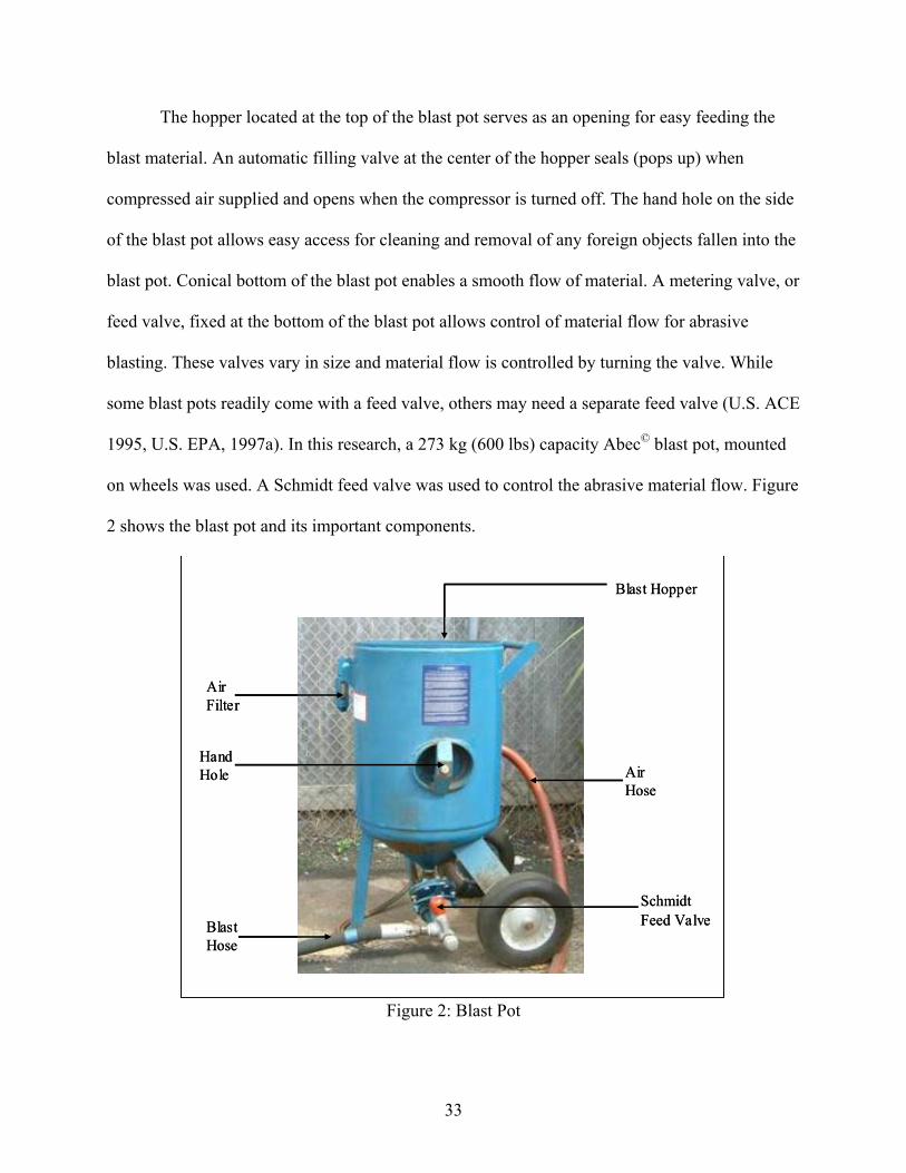
The hopper located at the top of the blast pot serves as an opening for easy feeding the
blast material. An automatic filling valve at the center of the hopper seals (pops up) when
compressed air supplied and opens when the compressor is turned off. The hand hole on the side
of the blast pot allows easy access for cleaning and removal of any foreign objects fallen into the
blast pot. Conical bottom of the blast pot enables a smooth flow of material. A metering valve, or
feed valve, fixed at the bottom of the blast pot allows control of material flow for abrasive
blasting. These valves vary in size and material flow is controlled by turning the valve. While
some blast pots readily come with a feed valve, others may need a separate feed valve (U.S. ACE
1995, U.S. EPA, 1997a). In this research, a 273 kg (600 lbs) capacity Abec© blast pot, mounted
on wheels was used. A Schmidt feed valve was used to control the abrasive material flow. Figure
2 shows the blast pot and its important components.
Blast Hopper
Hand Hole Air
Hose
Schmidt Feed Valve
Air Filter
Blast Hose
Blast Hopper
Hand Hole Air
Hose
Schmidt Feed Valve
Air Filter
Blast Hose
Figure 2: Blast Pot

34
4.2.2.2. Blast nozzle
Blast nozzle are identified by the inside diameter on the orifice and measured in
sixteenths of an inch (3/16-inch, 5/10-inch). These nozzles are assigned a number based on the
diameter. Selection on nozzle diameter depends on the capacity of air compressor and blast
pressure required. If the nozzle is too large, more volume of air must be supplied to achieve
required blast pressure. A Bazooka No.6 venturi type blast nozzle (3/8-inch or 9.5 mm diameter)
was used in this research.
4.2.2.3. Air hose and blast hose
The air hose is used to connect the compressor to the blast plot. The diameter of the hose
must be sufficient in preventing frictional losses and pressure drops, which decrease the process
efficiency. The blast hose is used to connect the blast pot to the blast nozzle and it carries both
abrasive material and compressed to the nozzle. This hose must be strong enough to carry the
material at high pressures.
4.2.2.4. Other blasting equipment
A secondary air supply unit was used to provide air to the blaster and moisture separators
were used to remove moisture from compressed air and secondary air supply. Personal protective
equipment included a respirator, helmet and heavy duty shoes.
4.2.3. Test Plates
Mild steel test plates of 2.5 x 1.5 m (8 x 5 feet) were used as base plates. The steel plates
were coated with a 1:1 volume mixture of commercially available Rust Oleum© Safety Yellow
paint and a thinner. Average thickness of the coating was calculated to be 0.73 mills assuming
average transfer efficiency of 50%. To support these plates during the experiment a panel cart
was used. The mount was also used to move the panels in and out of the test chamber.

35
4.2.4. Air Compressor
The air compressor provides the blast pressure required in dry abrasive blasting. The
compressor must be able to provide required blast pressures to achiever maximum productivity.
Sullair Model 375H© and Ingersoll Rand (power rating: 125-130 hp) compressors were used as
compressed air sources, which were able to provide a maximum blast pressure 150 PSI.
4.2.5. Exhaust Duct System
The exhaust duct system consisted of an exhaust duct and a fan. This system was used to
vent the emissions from the blasting operations in the test chamber to a particulate collection
system. Another important use of this systems was to collect sample PM emission factors. The
entrance of the duct system was fitted with a mesh to prevent too coarse particles from entering
the duct. The duct was 0.30 m (1 foot) in diameter with smooth inner surface to avoid
disturbances in the flow and designed according to EPA Method 1 (U.S. EPA 1997d). An
exhaust fan with maximum capacity of providing a volumetric flow of 5000 cfm was used to
vent the emissions by suction. An average of 3000 cfm was used in this research to vent
emissions from the test chamber. A sampling port was located on the exhaust duct to draw
sample exhaust gas for determining PM emission factors (Figure 3).

36
Figure 3: Exhaust Duct System (top left: From inside the test chamber, top right: from outside
the test chamber, bottom: duct connected to exhaust fan)
4.2.6. Stack Sampling System
U.S. EPA approved stack sampling system was used in this research. Components of this
system are mentioned in this section. The purpose of these components is discussed with the
sampling procedure.
4.2.6.1. Sampling train
The sampling train consisted of a tapered nozzle, sampling probe, filter holder, and a
series of four impingers, all of which are connected by connectors. The nozzle is used to draw
exhaust gas for PM sampling. For the sample to be representative, it must be drawn at isokinetic
conditions, i.e., the velocity of the gas in the stack and the velocity of the gas in the nozzle of the
sampling probe should be equal. Following the guidelines specified by U.S. EPA for stack
sampling, various nozzles were tested for isokinetic conditions and a nozzle with diameter of
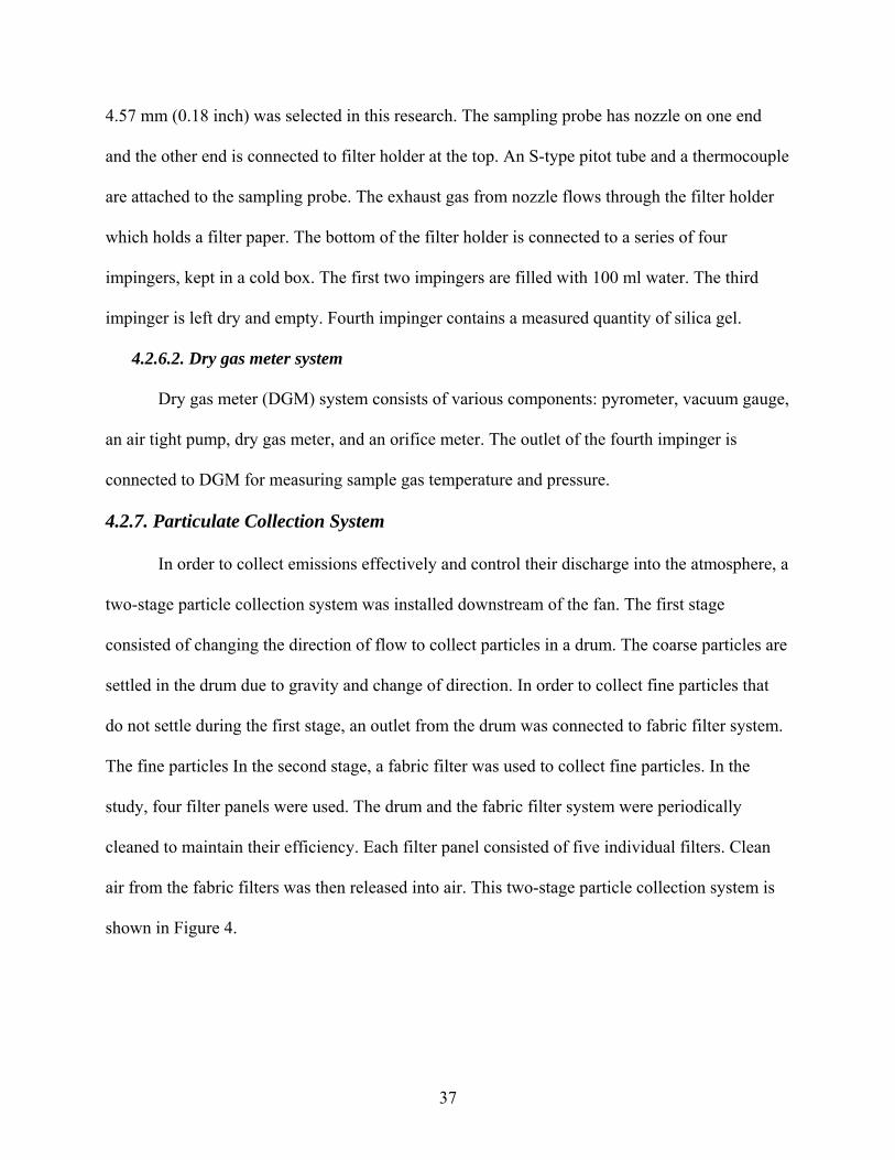
37
4.57 mm (0.18 inch) was selected in this research. The sampling probe has nozzle on one end
and the other end is connected to filter holder at the top. An S-type pitot tube and a thermocouple
are attached to the sampling probe. The exhaust gas from nozzle flows through the filter holder
which holds a filter paper. The bottom of the filter holder is connected to a series of four
impingers, kept in a cold box. The first two impingers are filled with 100 ml water. The third
impinger is left dry and empty. Fourth impinger contains a measured quantity of silica gel.
4.2.6.2. Dry gas meter system
Dry gas meter (DGM) system consists of various components: pyrometer, vacuum gauge,
an air tight pump, dry gas meter, and an orifice meter. The outlet of the fourth impinger is
connected to DGM for measuring sample gas temperature and pressure.
4.2.7. Particulate Collection System
In order to collect emissions effectively and control their discharge into the atmosphere, a
two-stage particle collection system was installed downstream of the fan. The first stage
consisted of changing the direction of flow to collect particles in a drum. The coarse particles are
settled in the drum due to gravity and change of direction. In order to collect fine particles that
do not settle during the first stage, an outlet from the drum was connected to fabric filter system.
The fine particles In the second stage, a fabric filter was used to collect fine particles. In the
study, four filter panels were used. The drum and the fabric filter system were periodically
cleaned to maintain their efficiency. Each filter panel consisted of five individual filters. Clean
air from the fabric filters was then released into air. This two-stage particle collection system is
shown in Figure 4.
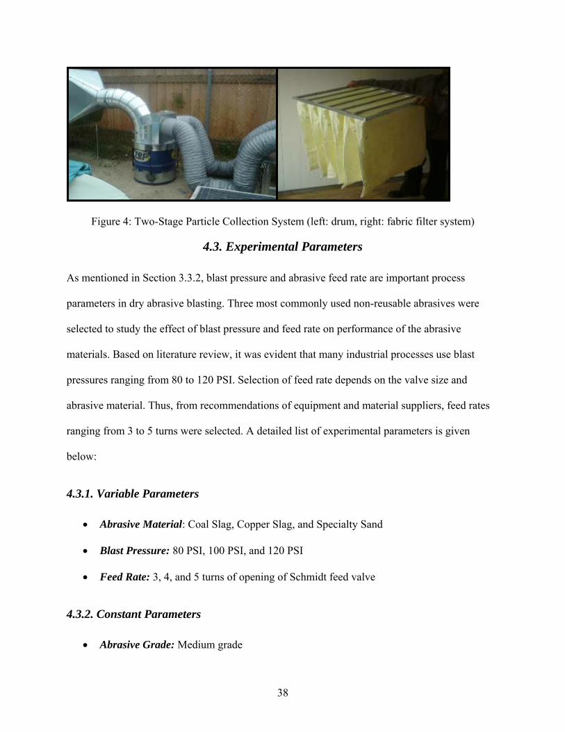
38
Figure 4: Two-Stage Particle Collection System (left: drum, right: fabric filter system)
4.3. Experimental Parameters
As mentioned in Section 3.3.2, blast pressure and abrasive feed rate are important process
parameters in dry abrasive blasting. Three most commonly used non-reusable abrasives were
selected to study the effect of blast pressure and feed rate on performance of the abrasive
materials. Based on literature review, it was evident that many industrial processes use blast
pressures ranging from 80 to 120 PSI. Selection of feed rate depends on the valve size and
abrasive material. Thus, from recommendations of equipment and material suppliers, feed rates
ranging from 3 to 5 turns were selected. A detailed list of experimental parameters is given
below:
4.3.1. Variable Parameters
• Abrasive Material: Coal Slag, Copper Slag, and Specialty Sand
• Blast Pressure: 80 PSI, 100 PSI, and 120 PSI
• Feed Rate: 3, 4, and 5 turns of opening of Schmidt feed valve
4.3.2. Constant Parameters
• Abrasive Grade: Medium grade

39
• Blast Nozzle: Bazooka No.6 nozzle with 9.5 mm diameter (venturi nozzle)
• Angle of Deflection: 900 (Nozzle held perpendicular to surface)
• Stand-off Distance: 12” was maintained between the test plate and the blast nozzle
• Exhaust Flow Rate: 3000 cfm (average volumetric flow rate)
• Surface Contamination: Paint with average thickness of 0.73 mill
• Surface Finish: Near-white finish (SP-10)
4.4. Experimental Procedure
The experimental procedure is explained in two sections: abrasive blasting and PM
sampling. PM sampling was performed while abrasive blasting was being carried out.
4.4.1. Abrasive Blasting
The test plates were coated with a 1:1 mixture of commercially available Rust Oleum©
Safety Yellow paint and a thinner. The paint was allowed to dry for 24 hours. Upon drying these
plates were moved inside the test chamber with the help of a cart. The inside of the blast pot was
checked for any foreign materials. Blast hose and air hose were connected to the blast pot and
feed valve was closed tightly. Stack sampling equipment was assembled. A measured quantity of
abrasive material (100 lbs in most cases) was added. Prior to adding, it was made sure that the
material was free of lumps and moisture. In case of presence of moisture, the material was well
dried and then added into the blast pot. Presence of lumps or moisture results in clogging the
valve and non-uniform flow of material.
The compressor was turned on and the blasting pressure was set to desired setting (80,
100, or 120 PSI). The Schmidt feed valve was adjusted to a desired number of turns (3, 4, or 5).
These blast pressure and feed rate settings were randomly chosen. The exhaust fan was turned on
to draw the emissions from the chamber. Blaster, provided with professional training for abrasive

40
blasting, then carried out blasting inside the chamber. During the whole time of abrasive
blasting, the test chamber was kept enclosed. Blasting was carried out until the blast pot was
emptied. The blaster visually ensured that the dwell time was sufficient to achieve a near-white
surface finish. The compressor was then turned off and feed valve was closed. The time taken for
each test run was recorded using a stopwatch and the area cleaned was measured using a
measuring tape. For each combination of pressure and feed rate, three test runs were carried out
to minimize experimental errors and test the repeatability of the results. Thus a total number of
27 experiments were performed for each material.
4.4.2. PM Sampling
As the blasting was carried out inside the chamber, samples were drawn isokinetically
through the sampling probe. A brief procedure for PM sampling is discussed in this section and a
detailed procedure is available at http://www.epa.gov/ttn/emc.
4.4.2.1. Selection of sampling ports and traverse points
Based on the guidelines provided in EPA Method 1 (U.S. EPA 1997d), in order to
minimize the effect of flow disturbances on sampling, a sampling port was located at point at
least 8 diameters upstream (test chamber) and 2 diameters downstream (exhaust fan). For a
circular duct with a diameter between 0.30 and 0.61 meter (12 and 24 inches), a total of eight
traverse points must be selected. The location of these traverse points, along the plane
perpendicular to direction of flow of exhaust gas, was calculated as per the guidelines and
marked on sampling probe with a heat resistant tape to denote the distance into the duct for each
traverse point. The purposes of sampling at various locations in the duct were to measure average
stack gas velocity and obtain a representative sample for PM emissions.

41
4.4.2.2. Stack gas velocity and flow rate measurements
The average gas velocity in the duct was determined from measurement of average
velocity head with the S-type pitot tube attached to the sampling probe. A temperature sensor
attached to the sampling probe was used to measure the exhaust gas temperature at the traverse
points. Atmospheric pressure was recorded from a nearby National Weather Service station.
Leak checks were performed once the sampling train was assembled. The sample probe was
sufficiently heated to prevent condensation of moisture present in the exhaust gas. At each
traverse point, exhaust gas sample was collected for two minutes. Thus, total sampling time was
sixteen minutes for each of the test runs. At the end of 16 minutes, sampling probe was
withdrawn, and the exhaust fan was turned off. The measurements made at each traverse point,
according EPA Method 2 (U.S. EPA 1997e), and equations used to calculate the stack gas
velocity and flow rate for each experiment are given in Appendix A.
4.4.2.3. Determination of moisture content
The moisture content in the exhaust was determined according to the guidelines in EPA
Method 4 (U.S. EPA 1997f). The exhaust gas, after passing through the filter paper is passed
through a series of four impingers (first two filled with 100 ml water, third left empty and fourth
filled with measured quantity of silica gel) to collect moisture present in the exhaust gas. These
impingers were placed in an ice bath containing crushed ice, which helps in condensing the
moisture. The weights of four impingers were recorded before and after each experiment. The
increase in weight of each impinger was used to calculate weight of water collected. The exhaust
gas was then passed through dry gas meter to determine volume and temperature of the gas.
Moisture content was calculated using the equations given in EPA Method 4. These equations
and calculations for each experiment are presented in Appendix A.

42
4.4.2.4. Determination of PM emissions
The particles were collected on a pre-weighed Whatman No. 10 filter paper that was
already desiccated to eliminate moisture. The filter assembly box was maintained at a
temperature of 120 ± 15°C to collect particulate matter from the sample gas stream while
preventing moisture condensation. Once the sample was collected, the filter paper was removed
from the filter box and placed in a dessicator. PM from the probe was collected in a beaker by
rinsing the probe with acetone. The final weights of PM in filter paper and beaker were recorded
after dessicating them for 24 hours. The sum of the weights of both containers was used to
determine the actual mass of emissions in the stack gas using the equations in EPA Method 5
(U.S. EPA 1997g). The actual mass of PM collected in sample exhaust gas, equations used and
total mass of PM in the exhaust gas for each experiment are presented in Appendix A.
4.5. Statistical Analysis
The data collected from field measurements was transferred in Excel for analysis. Mean
and standard deviation of three experimental runs were calculated were for each combination of
blast pressure and feed rate. This data is presented in Section 5. In order to develop predictive
models to estimate emission factors, productivity and consumption (performance parameters) at
intermediate blast pressure and feed rate conditions (process parameters), multiple regression
analysis was performed. Two-dimensional and three dimensional models were developed. Two-
dimensional models were used to study the effect of a single process condition on performance
parameter. In addition, these models were used compare the performance of the three abrasive
materials at various operating conditions. DataFit@, a curve fitting application, was used for
developing three-dimensional models. These models were used to study the simultaneous effect
of process parameters on performance parameters.

43
The best-fit models were selected based on the physical phenomenon discussed in
Literature Review, R2, and continuity of the curve (in case of 3-D models). The R² value, also
known as the Coefficient of Determination, is an indicator that ranges in value from 0 to 1. This
coefficient reveals how closely the estimated values for the regression correspond to the actual
data. A regression is most reliable when its R² value is at or near 1 (Kleinbaum 1992, McBean
and Rovers 1998). The value for R² was determined using the following equations:
Residual = (Yi – Ŷi)
Sum of Residuals = ∑ (Yi – Ŷi)
Average Residual = ∑ (Yi – Ŷi) / n
Residual Sum of Squares, SSE = ∑ (Yi – Ŷi)2
Regression Sum of Squares, SSR, ∑ (Ŷi -Yi)2
Total Sum of Squares, SST = SSE + SSR,
Coefficient of Multiple Determination, R2 = SSR / SST
Two-way ANOVA was used to test the significance of the regression model. F static was
calculated for H0 : a = 0, b = 0, c = 0, d = 0, e = 0, and f = 0, where a, b, c, d, e, and f are
coefficients in the regression model. Null hypothesis (H0) was rejected if Prob(F) < 0.025.
Prob(F) = 0 means the probability of obtaining data equal to more extreme under the null
hypothesis is zero. In addition, t static was calculated for H0: a = 0, b = 0, c = 0, d = 0, e = 0, or f
= 0 to test the significance of each coefficient. Null hypothesis was rejected if Prob(t) < 0.05.
44
Since the analysis was performed assuming normal distribution of the data, residual plots
were used check this assumption. The following scatter diagrams were plotted to check the
normal distribution of the data:
• Residuals vs. Predicted Y: the residuals should not show any pattern or structure
for normally distributed data.
• Residual Normality Plot: The plot must be a straight line for normally distributed
data.
In addition, predicted values of performance parameters were plotted with observed
values.
Detailed results of the statistical analysis of the data, ANOVA table, confidence intervals,
and scatter diagrams are included in Appendix B. The Results and Discussion section includes
the 2-D and 3-D models which will help understanding the effect of process parameters on
performance parameters and compare the performance of three abrasive materials. The equations
developed for calculating emission factors, productivity, and consumption at intermediate blast
pressure and feed rate are presented in Section 5 along with the R2 values and coefficients for
99% confidence levels. The confidence intervals are presented in Appendix B.

45
5. Results and Discussion
The fundamental goals of this study was to evaluate the performance of three non-
reusable abrasives and study the effect of blast pressure and feed rate on performance of each
material. In order to achieve these goals, the following parameters were calculated for each
experiment performed:
• Emission Factors:
o kg TPM per unit area cleaned: Mass of TPM emitted (kg) / Area cleaned
(m2)
o kg TPM per unit mass of abrasive: Mass of TPM emitted (kg) / Quantity
of abrasive used (kg)
• Productivity:
o Area cleaned per unit time: Area cleaned (m2) / Blasting time (hr)
• Consumption:
o Mass of abrasive per unit area: Quantity of abrasive used (kg) / Area
Cleaned (m2)
It must be noted that the emission factors determined in this research correspond to
uncontrolled emissions since samples were collected prior to applying any emission controls.
Predictive mathematical models were developed to determine these parameters based on blast
pressure and abrasive feed rate. Detailed information on the data collected, and calculation PM
emissions is presented in Appendix A. The detailed results of statistical analysis performed for
this data is presented in Appendix B. The results of the experiments, variation of performance of
each abrasive with respect to blast pressure and feed rate, and predictive models developed are
presented in this section.

46
Table 5: Experimental Results for Coal Slag
Pressure Feed Rate
Abrasive Quantity
Blasting Time
Area Cleaned
TPM Emissions Productivity Consumption
Emission Factor 1
Emission Factor 2
PSI Turns lbs min ft2 g m2/hr kg/m2 kg/m2 kg/kg 120 3 100 6 13.0 3604 12.08 37.57 2.984 0.0794 120 3 100 6 12.0 3590 11.15 40.70 3.221 0.0791 120 3 100 6 12.0 3562 11.15 40.70 3.195 0.0785 120 4 100 5 17.0 3349 18.95 28.73 2.121 0.0738 120 4 100 6 17.5 3388 16.26 27.91 2.084 0.0747 120 4 100 6 17.0 3371 15.79 28.73 2.135 0.0743 120 5 150 7 17.0 5526 13.54 43.10 3.499 0.0812 120 5 150 7 18.0 5839 14.33 40.70 3.492 0.0858 120 5 150 7 18.0 5780 14.33 40.70 3.456 0.0849 100 3 100 7 13.0 2849 10.35 37.57 2.358 0.0628 100 3 100 7 12.5 2693 9.95 39.07 2.319 0.0594 100 3 100 8 12.5 2785 8.71 39.07 2.398 0.0614 100 4 120 5 12.5 2345 13.94 46.88 2.019 0.0431 100 4 120 7 18.0 3327 14.33 32.56 1.990 0.0611 100 4 120 7 17.0 3172 13.54 34.48 2.009 0.0583 100 5 120 6 12.0 3372 11.15 48.84 3.025 0.0619 100 5 80 4 8.0 2368 11.15 48.84 3.186 0.0652 100 5 120 6 12.5 3499 11.61 46.88 3.013 0.0643 80 3 30 4 6.0 1045 8.36 24.42 1.875 0.0768 80 3 100 11 15.0 2679 7.60 32.56 1.922 0.0590 80 3 70 6 9.5 1634 8.83 35.98 1.851 0.0514 80 4 100 7 16.5 2003 13.14 29.60 1.307 0.0441 80 4 100 7 16.0 2041 12.74 30.52 1.373 0.0450 80 4 120 11 24.0 2912 12.16 24.42 1.306 0.0535 80 5 100 7 13.0 3004 10.35 37.57 2.488 0.0662 80 5 100 7 12.0 2689 9.56 40.70 2.412 0.0593 80 5 80 5 9.5 2160 10.59 41.13 2.448 0.0595
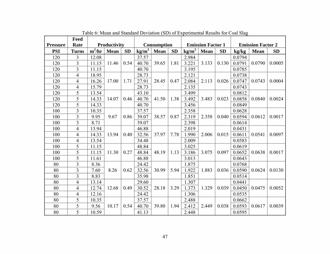
47
Table 6: Mean and Standard Deviation (SD) of Experimental Results for Coal Slag
Pressure Feed Rate Productivity Consumption Emission Factor 1 Emission Factor 2
PSI Turns m2/hr Mean SD kg/m2 Mean SD kg/m2 Mean SD kg/kg Mean SD 120 3 12.08 37.57 2.984 0.0794120 3 11.15 40.70 3.221 0.0791120 3 11.15
11.46 0.5440.70
39.65 1.813.195
3.133 0.1300.0785
0.0790 0.0005
120 4 18.95 28.73 2.121 0.0738120 4 16.26 27.91 2.084 0.0747120 4 15.79
17.00 1.7128.73
28.45 0.472.135
2.113 0.0260.0743
0.0743 0.0004
120 5 13.54 43.10 3.499 0.0812120 5 14.33 40.70 3.492 0.0858120 5 14.33
14.07 0.4640.70
41.50 1.383.456
3.483 0.0230.0849
0.0840 0.0024
100 3 10.35 37.57 2.358 0.0628100 3 9.95 39.07 2.319 0.0594100 3 8.71
9.67 0.8639.07
38.57 0.872.398
2.358 0.0400.0614
0.0612 0.0017
100 4 13.94 46.88 2.019 0.0431100 4 14.33 32.56 1.990 0.0611100 4 13.54
13.94 0.4034.48
37.97 7.782.009
2.006 0.0150.0583
0.0541 0.0097
100 5 11.15 48.84 3.025 0.0619100 5 11.15 48.84 3.186 0.0652100 5 11.61
11.30 0.2746.88
48.19 1.133.013
3.075 0.0970.0643
0.0638 0.0017
80 3 8.36 24.42 1.875 0.076880 3 7.60 32.56 1.922 0.059080 3 8.83
8.26 0.6235.98
30.99 5.941.851
1.883 0.0360.0514
0.0624 0.0130
80 4 13.14 29.60 1.307 0.044180 4 12.74 30.52 1.373 0.045080 4 12.16
12.68 0.4924.42
28.18 3.291.306
1.329 0.0390.0535
0.0475 0.0052
80 5 10.35 37.57 2.488 0.066280 5 9.56 40.70 2.412 0.059380 5 10.59
10.17 0.5441.13
39.80 1.942.448
2.449 0.0380.0595
0.0617 0.0039

48
Table 7: Experimental Results for Copper Slag
Pressure Feed Rate
Abrasive Quantity
Blasting Time
Area Cleaned
TPM Emissions Productivity Consumption
Emission Factor 1
Emission Factor 2
PSI Turns lbs min ft2 g m2/hr kg/m2 kg/m2 kg/kg 120 3 100 7 8.5 2060 6.77 57.46 2.609 0.0454 120 3 100 8 9.0 2165 6.27 54.26 2.589 0.0477 120 3 50 5 6.0 1431 6.69 40.70 2.567 0.0631 120 4 150 10 20.0 2725 11.15 36.63 1.466 0.0400 120 4 100 6 12.0 1754 11.15 40.70 1.573 0.0387 120 4 50 4 8.0 1163 11.15 30.52 1.565 0.0513 120 5 120 6 10.0 2823 9.29 58.61 3.039 0.0518 120 5 80 4 7.0 1962 9.75 55.82 3.017 0.0540 120 5 100 4 7.3 2053 10.10 67.36 3.048 0.0452 100 3 100 8 13.5 2463 9.41 36.17 1.964 0.0543 100 3 50 4 7.0 1256 9.75 34.89 1.932 0.0554 100 3 75 6 10.3 1859.5 9.58 35.53 1.948 0.0548 100 4 150 7 18.0 2946 14.33 40.70 1.762 0.0433 100 4 150 7 17.8 2938 14.18 41.13 1.775 0.0432 100 4 120 6 15.0 2438 13.94 39.07 1.749 0.0448 100 5 120 8 15.8 3105 10.97 37.21 2.122 0.0570 100 5 50 4 8.0 1538 11.15 30.52 2.070 0.0678 100 5 50 4 8.0 1518 11.15 30.52 2.043 0.0669 80 3 50 6 6.0 1560 5.57 40.70 2.800 0.0688 80 3 50 7 6.5 1581 5.18 37.57 2.618 0.0697 80 3 50 6 6.5 1591 6.04 37.57 2.634 0.0701 80 4 150 12 19.0 3729 8.83 38.56 2.113 0.0548 80 4 100 6 9.8 1861 9.06 50.09 2.055 0.0410 80 4 125 9 14.4 2795 8.94 44.33 2.084 0.0479 80 5 80 8 9.0 2957 6.27 43.41 3.537 0.0815 80 5 80 6 7.0 2306 6.50 55.82 3.546 0.0635 80 5 80 7 8.0 2631.5 6.39 49.62 3.541 0.0725

49
Table 8: Mean and Standard Deviation (SD) of Experimental Results for Copper Slag
Pressure Feed Rate Productivity Consumption Emission Factor 1 Emission Factor 2
PSI Turns m2/hr Mean SD kg/m2 Mean SD kg/m2 Mean SD kg/kg Mean SD 120 3 6.77 57.46 2.609 0.0454120 3 6.27 54.26 2.589 0.0477120 3 6.69
6.58 0.2740.70
50.81 8.902.567
2.588 0.0210.0631
0.0521 0.0096
120 4 11.15 36.63 1.466 0.0400120 4 11.15 40.70 1.573 0.0387120 4 11.15
11.15 0.0030.52
35.95 5.121.565
1.535 0.0590.0513
0.0433 0.0069
120 5 9.29 58.61 3.039 0.0518120 5 9.75 55.82 3.017 0.0540120 5 10.10
9.72 0.4167.36
60.60 6.023.048
3.035 0.0160.0452
0.0504 0.0046
100 3 9.41 36.17 1.964 0.0543100 3 9.75 34.89 1.932 0.0554100 3 9.58
9.58 0.1735.53
35.53 0.641.948
1.948 0.0160.0548
0.0548 0.0006
100 4 14.33 40.70 1.762 0.0433100 4 14.18 41.13 1.775 0.0432100 4 13.94
14.15 0.2039.07
40.30 1.081.749
1.762 0.0130.0448
0.0437 0.0009
100 5 10.97 37.21 2.122 0.0570100 5 11.15 30.52 2.070 0.0678100 5 11.15
11.09 0.1030.52
32.75 3.862.043
2.078 0.0400.0669
0.0639 0.0060
80 3 5.57 40.70 2.800 0.068880 3 5.18 37.57 2.618 0.069780 3 6.04
5.60 0.4337.57
38.61 1.812.634
2.684 0.1010.0701
0.0695 0.0007
80 4 8.83 38.56 2.113 0.054880 4 9.06 50.09 2.055 0.041080 4 8.94
8.94 0.1244.33
44.32 5.772.084
2.084 0.0290.0479
0.0479 0.0069
80 5 6.27 43.41 3.537 0.081580 5 6.50 55.82 3.546 0.063580 5 6.39
6.39 0.1249.62
49.62 6.203.541
3.541 0.0040.0725
0.0725 0.0090

50
Table 9: Experimental Results for Specialty Sand
Pressure Feed Rate
Abrasive Quantity
Blasting Time
Area Cleaned
TPM Emissions Productivity Consumption
Emission Factor 1
Emission Factor 2
PSI Turns lbs min ft2 g m2/hr kg/m2 kg/m2 kg/kg 120 3 50 6 11.5 3034 10.68 21.23 2.840 0.1337 120 3 100 8 15.0 4242 10.45 32.56 3.044 0.0935 120 3 50 3 5.8 1615 10.68 42.47 3.024 0.0712 120 4 50 4 10.0 4005 13.94 24.42 4.311 0.1766 120 4 50 3 7.8 3611 14.40 31.51 5.015 0.1592 120 4 100 9 22.0 9578 13.63 22.20 4.687 0.2111 120 5 100 7 22.5 8042 17.92 21.70 3.847 0.1772 120 5 100 5 15.0 5161 16.72 32.56 3.704 0.1137 120 5 100 6 18.8 6586 17.42 26.05 3.781 0.1452 100 3 50 4 10.5 1298 14.63 23.26 1.330 0.0572 100 3 50 4 10.0 1365 13.94 24.42 1.469 0.0601 100 3 50 3 7.5 681 13.94 32.56 0.976 0.0300 100 4 50 4 11.8 3214 16.37 20.78 2.944 0.1417 100 4 50 4 12.0 3298 16.72 20.35 2.958 0.1454 100 4 100 7 21.5 6165 17.12 22.71 3.087 0.1359 100 5 50 4 6.5 2148 9.06 37.57 3.556 0.0947 100 5 50 3 5.3 1977 9.75 46.51 4.054 0.0871 100 5 100 10 17.0 5722 9.48 28.73 3.623 0.1261 80 3 50 4 8.8 846 12.19 27.91 1.041 0.0373 80 3 100 8 14.5 1500 10.10 33.68 1.114 0.0331 80 3 100 8 15.0 1679 10.45 32.56 1.204 0.0370 80 4 50 4 8.8 1116 12.19 27.91 1.373 0.0492 80 4 50 5 10.0 1449 11.15 24.42 1.560 0.0639 80 4 100 8 18.0 2464 12.54 27.13 1.474 0.0543 80 5 50 5 7.1 1480 7.94 34.27 2.236 0.0652 80 5 50 5 8.0 1824 8.92 30.52 2.453 0.0804 80 5 100 8 13.8 3228 9.58 35.52 2.526 0.0711

51
Table 10: Mean and Standard Deviation (SD) of Experimental Results for Specialty Sand
Pressure Feed Rate Productivity Consumption Emission Factor 1 Emission Factor 2
PSI Turns m2/hr Mean SD kg/m2 Mean SD kg/m2 Mean SD kg/kg Mean SD 120 3 10.68 21.23 2.840 0.1337120 3 10.45 32.56 3.044 0.0935120 3 10.68
10.61 0.1342.47
32.09 10.633.024
2.969 0.1130.0712
0.0995 0.0317
120 4 13.94 24.42 4.311 0.1766120 4 14.40 31.51 5.015 0.1592120 4 13.63
13.99 0.3922.20
26.04 4.86 4.687
4.671 0.3520.2111
0.1823 0.0264
120 5 17.92 21.70 3.847 0.1772120 5 16.72 32.56 3.704 0.1137120 5 17.42
17.35 0.6026.05
26.77 5.46 3.781
3.777 0.0720.1452
0.1454 0.0317
100 3 14.63 23.26 1.330 0.0572100 3 13.94 24.42 1.469 0.0601100 3 13.94
14.17 0.4032.56
26.75 5.07 0.976
1.259 0.2540.0300
0.0491 0.0166
100 4 16.37 20.78 2.944 0.1417100 4 16.72 20.35 2.958 0.1454100 4 17.12
16.74 0.3722.71
21.28 1.26 3.087
2.996 0.0790.1359
0.1410 0.0048
100 5 9.06 37.57 3.556 0.0947100 5 9.75 46.51 4.054 0.0871100 5 9.48
9.43 0.3528.73
37.60 8.89 3.623
3.744 0.2700.1261
0.1026 0.0207
80 3 12.19 27.91 1.041 0.037380 3 10.10 33.68 1.114 0.033180 3 10.45
10.92 1.1232.56
31.38 3.06 1.204
1.120 0.0820.0370
0.0358 0.0024
80 4 12.19 27.91 1.373 0.049280 4 11.15 24.42 1.560 0.063980 4 12.54
11.96 0.7327.13
26.49 1.83 1.474
1.469 0.0930.0543
0.0558 0.0074
80 5 7.94 34.27 2.236 0.065280 5 8.92 30.52 2.453 0.080480 5 9.58
8.81 0.8235.52
33.44 2.60 2.526
2.405 0.1510.0711
0.0723 0.0076

52
5.1. Emission Factors
5.1.1. Emission Factors in kg/m2
5.1.1.1. Variation of emission factors (kg/m2) with pressure
Velocity of abrasive particles is determined by blast pressure. Higher the pressure, greater
will be the velocity and hence greater impact on base plate. Although this may increase
productivity, at very high velocity, the abrasive particles suffer more damage, thus breakdown
into smaller particles. This causes increased emissions at high pressure. Figure 5 shows the
variation of emission factors (kg/m2) with pressure at 3 turns of feed rate. It was observed that
emission factors increased with pressure for coal slag and specialty sand. This may be due to
more number of particles undergoing damage with increase in pressure.
Variation of Emission Factors (kg/m2) with Pressure at 3 Turns
Coal Slagy = 0.0004x2 - 0.0446x + 3.0329
R2 = 0.98
Copper Slagy = 0.0017x2 - 0.3463x + 19.382
R2 = 0.98
Specialty Sandy = 0.002x2 - 0.3467x + 16.28
R2 = 0.970.0
1.0
2.0
3.0
4.0
70 80 90 100 110 120 130
Pressure (PSI)
Em
issi
on F
acto
rs (k
g/m
2 )
Coal SlagCopper SlagSpecialty Sand
Figure 5: Variation of Emission Factors (kg/m2) with Pressure at 3 Turns
In case of copper slag, emission factors decreased with increase in pressure from 80 PSI
to 100 PSI and then increased with further increase in pressure. This may be because at lower
pressure, although emissions may be less, emission factors will be high because of less

53
productivity and more consumption at lower velocity. It can be observed from the graph that at
lower pressure, emission factors varied significantly from one material to another, highest being
copper slag. At very high pressure, all three materials have less comparable emission factors,
especially for coal slag and specialty sand. The regression equations developed and
corresponding R2 values are shown in Figure 5.
Variation of emission factors (kg/m2) with pressure at 4 turns of feed rate is shown in
Figure 6. Emission factors for coal slag and specialty sand increased with pressure similar to the
variation at 3 turns. However, for copper slag, emission factors decreased with increase in
pressure.
Variation of Emission Factors (kg/m2) with Pressure at 4 Turns
Coal Slagy = -0.0007x2 + 0.1631x - 7.1236
R2 = 0.99
Copper Slagy = 0.0001x2 - 0.0373x + 4.3149
R2 = 0.98
Specialty Sandy = 0.0002x2 + 0.0433x - 3.1696
R2 = 0.980.0
1.0
2.0
3.0
4.0
5.0
6.0
70 80 90 100 110 120 130
Pressure (PSI)
Em
issi
on F
acto
rs (k
g/m
2 )
Coal SlagCopper SlagSpecialty Sand
Figure 6: Variation of Emission Factors (kg/m2) with Pressure at 4 Turns
It can be observed from Figure 6 that increase in emission factors for specialty sand was
significantly higher while in case of coal slag and copper slag, a slight variation of emission
factors was observed. R2 values obtained for the three materials were very close (0.98 and 0.99)
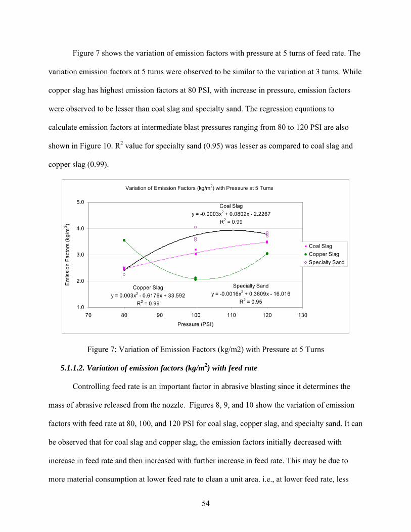
54
Figure 7 shows the variation of emission factors with pressure at 5 turns of feed rate. The
variation emission factors at 5 turns were observed to be similar to the variation at 3 turns. While
copper slag has highest emission factors at 80 PSI, with increase in pressure, emission factors
were observed to be lesser than coal slag and specialty sand. The regression equations to
calculate emission factors at intermediate blast pressures ranging from 80 to 120 PSI are also
shown in Figure 10. R2 value for specialty sand (0.95) was lesser as compared to coal slag and
copper slag (0.99).
Variation of Emission Factors (kg/m2) with Pressure at 5 Turns
Coal Slagy = -0.0003x2 + 0.0802x - 2.2267
R2 = 0.99
Copper Slagy = 0.003x2 - 0.6176x + 33.592
R2 = 0.99
Specialty Sandy = -0.0016x2 + 0.3609x - 16.016
R2 = 0.951.0
2.0
3.0
4.0
5.0
70 80 90 100 110 120 130
Pressure (PSI)
Em
issi
on F
acto
rs (k
g/m
2 )
Coal SlagCopper SlagSpecialty Sand
Figure 7: Variation of Emission Factors (kg/m2) with Pressure at 5 Turns 5.1.1.2. Variation of emission factors (kg/m2) with feed rate
Controlling feed rate is an important factor in abrasive blasting since it determines the
mass of abrasive released from the nozzle. Figures 8, 9, and 10 show the variation of emission
factors with feed rate at 80, 100, and 120 PSI for coal slag, copper slag, and specialty sand. It can
be observed that for coal slag and copper slag, the emission factors initially decreased with
increase in feed rate and then increased with further increase in feed rate. This may be due to
more material consumption at lower feed rate to clean a unit area. i.e., at lower feed rate, less

55
number of particles impacts the unit surface and consumes more material to achieve desired
surface finish.
Variation of Emission Factors (kg/m2) with Feed Rate at 80 PSI
Coal Slagy = 0.8394x2 - 6.4342x + 13.635
R2 = 0.99
Copper Slagy = 1.0287x2 - 7.8007x + 16.828
R2 = 0.99
Specialty Sandy = 0.2935x2 - 1.7054x + 3.5945
R2 = 0.970.0
1.0
2.0
3.0
4.0
2 3 4 5 6
Feed Rate (number of turns)
Em
issi
on F
acto
rs (k
g/m
2 )
Coal SlagCopper Slag
Specialty Sand
Figure 8: Variation of Emission Factors (kg/m2) with Feed Rate at 80 PSI
With increase in feed rate, more uniform flow of material occurs and less material is
consumed to clean a unit area, thus resulting in less emission factors. However, at very high feed
rates, the particles traveling from the nozzle interact with the rebounding particles from the base
plate and breakdown resulting in higher emissions and consuming more material. In addition, at
high feed rates, flow of material may turbulent rather than uniform. This increases emission
factors with increase in feed rate.
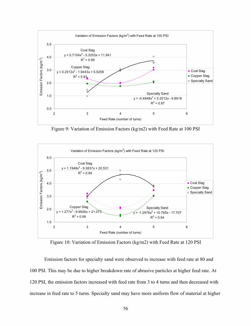
56
Variation of Emission Factors (kg/m2) with Feed Rate at 100 PSI
Coal Slagy = 0.7104x2 - 5.3253x + 11.941
R2 = 0.99
Copper Slagy = 0.2512x2 - 1.9443x + 5.5209
R2 = 0.97
Specialty Sandy = -0.4948x2 + 5.2012x - 9.8918
R2 = 0.970.0
1.0
2.0
3.0
4.0
5.0
2 3 4 5 6
Feed Rate (number of turns)
Em
issi
on F
acto
rs (k
g/m
2 )
Coal SlagCopper SlagSpecialty Sand
Figure 9: Variation of Emission Factors (kg/m2) with Feed Rate at 100 PSI
Variation of Emission Factors (kg/m2) with Feed Rate at 120 PSI
Coal Slagy = 1.1948x2 - 9.3837x + 20.531
R2 = 0.99
Copper Slagy = 1.277x2 - 9.9926x + 21.073
R2 = 0.99
Specialty Sandy = -1.2976x2 + 10.785x - 17.707
R2 = 0.941.0
2.0
3.0
4.0
5.0
6.0
2 3 4 5 6
Feed Rate (number of turns)
Em
issi
on F
acto
rs (k
g/m
2 )
Coal SlagCopper SlagSpecialty Sand
Figure 10: Variation of Emission Factors (kg/m2) with Feed Rate at 120 PSI
Emission factors for specialty sand were observed to increase with feed rate at 80 and
100 PSI. This may be due to higher breakdown rate of abrasive particles at higher feed rate. At
120 PSI, the emission factors increased with feed rate from 3 to 4 turns and then decreased with
increase in feed rate to 5 turns. Specialty sand may have more uniform flow of material at higher

57
pressure and feed rate conditions, resulting in lower emissions which can be observed from
Figures 7 and 10. At 80 PSI, copper slag has higher emission factors than coal slag and at 100
and 120 PSI, copper slag has lower emission factors than coal slag. In case of sand, lower
emission factors were observed at low pressure (80 PSI). The regression equations to determine
emission factors at intermediate feed rates for blast pressures of 80, 100, and 120 PSI are also
shown in Figures 8, 9, and 10 respectively.
5.1.1.3. Variation of emission factors (kg/m2) with pressure and feed rate
The variations and equations discussed above depict either effect of pressure on
emissions at a given feed rate or effect of feed rate at a specific pressure. In order to study
simultaneous effects of both, pressure and feed rate on emissions, three-dimensional models
were developed. Datafit © curve fitting application was used for regression analysis and for
plotting three-dimensional charts. Figure 11, 12, and 13 demonstrates the variation of emission
factors with pressure and feed rate for coal slag, copper slag, and specialty sand respectively.
Figure 11: Coal Slag - Variation of Emission Factors (kg/m2) with Pressure and Feed Rate

58
Figure 12: .Copper Slag - Variation of Emission Factors (kg/m2) with Pressure and Feed Rate
Figure 13: Specialty Sand - Variation of Emission Factors (kg/m2) with Pressure and Feed Rate
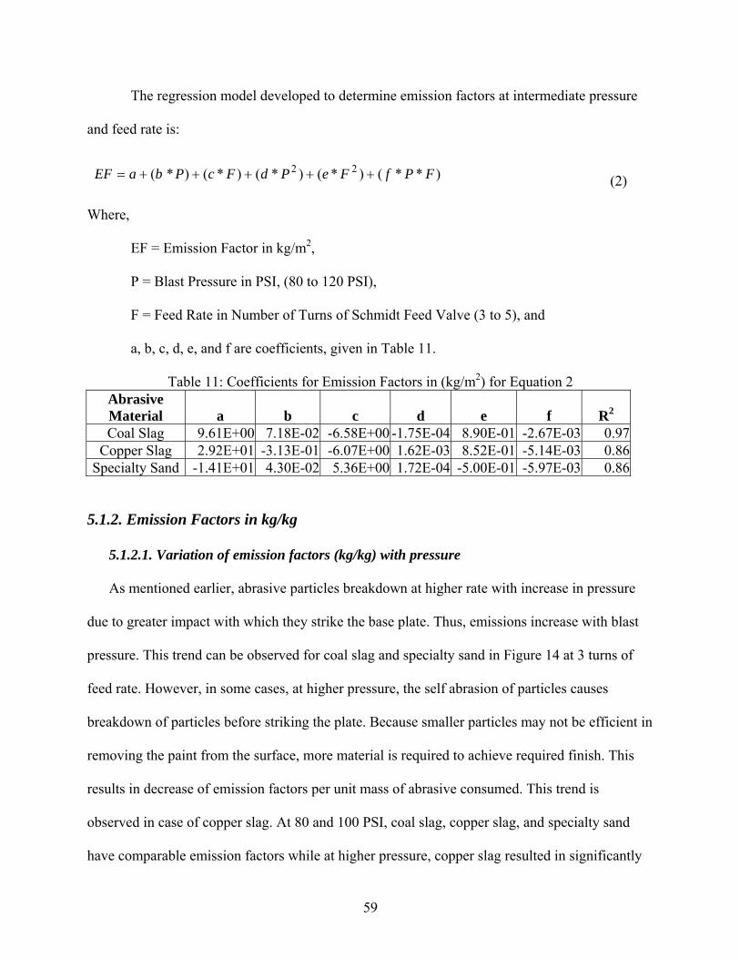
59
The regression model developed to determine emission factors at intermediate pressure
and feed rate is:
)**()*()*()*()*( 22 FPfFePdFcPbaEF +++++= (2)
Where,
EF = Emission Factor in kg/m2,
P = Blast Pressure in PSI, (80 to 120 PSI),
F = Feed Rate in Number of Turns of Schmidt Feed Valve (3 to 5), and
a, b, c, d, e, and f are coefficients, given in Table 11.
Table 11: Coefficients for Emission Factors in (kg/m2) for Equation 2 Abrasive Material a b c d e f R2 Coal Slag 9.61E+00 7.18E-02 -6.58E+00 -1.75E-04 8.90E-01 -2.67E-03 0.97
Copper Slag 2.92E+01 -3.13E-01 -6.07E+00 1.62E-03 8.52E-01 -5.14E-03 0.86Specialty Sand -1.41E+01 4.30E-02 5.36E+00 1.72E-04 -5.00E-01 -5.97E-03 0.86
5.1.2. Emission Factors in kg/kg
5.1.2.1. Variation of emission factors (kg/kg) with pressure
As mentioned earlier, abrasive particles breakdown at higher rate with increase in pressure
due to greater impact with which they strike the base plate. Thus, emissions increase with blast
pressure. This trend can be observed for coal slag and specialty sand in Figure 14 at 3 turns of
feed rate. However, in some cases, at higher pressure, the self abrasion of particles causes
breakdown of particles before striking the plate. Because smaller particles may not be efficient in
removing the paint from the surface, more material is required to achieve required finish. This
results in decrease of emission factors per unit mass of abrasive consumed. This trend is
observed in case of copper slag. At 80 and 100 PSI, coal slag, copper slag, and specialty sand
have comparable emission factors while at higher pressure, copper slag resulted in significantly

60
lesser emission factors. The R2 values obtained from the regression analysis were lower for coal
slag and specialty sand.
Variation of Emission Factors (kg/kg) with Pressure at 3 Turns
Coal Slagy = 2E-05x2 - 0.0044x + 0.2584
R2 = 0.63Copper Slag
y = 8E-06x2 - 0.0022x + 0.1926R2 = 0.99
Specialty Sandy = 5E-05x2 - 0.0077x + 0.3529
R2 = 0.720.00
0.04
0.08
0.12
0.16
70 80 90 100 110 120 130
Pressure (PSI)
Em
issi
on F
acto
rs (k
g/kg
)
Coal SlagCopper SlagSpecialty Sand
Figure 14: Variation of Emission Factors (kg/kg) with Pressure at 3 turns
Figure 15 shows the variation of emission factors with pressure at 4 turns of feed rate.
Similar to variation at 3 turns, emission factors for coal slag and specialty sand. Increase in
emission factors for specialty sand was considerably higher as compared to coal slag.
In case of copper slag, emission factors decreased with increase in blast pressure, which may be
sue to the effect of self abrasion of particles as explained earlier. At 80 PSI, all three materials
were observed to have almost same emission factors. With increase in pressure, emission factors
for specialty sand increased significantly than for coal slag and copper slag. At 120 PSI, copper
slag was observed to have the lowest emission factors and specialty sand, highest emission
factors. Regression equations to calculate emission factors at intermediate blast pressure are also
given in Figure 15. Copper slag had notably lower R2 (0.48) compared to coal slag and specialty
sand.

61
Variation of Emission Factors (kg/kg) with Pressure at 4 Turns
Coal Slagy = 2E-05x2 - 0.0027x + 0.1561
R2 = 0.83
Copper Slagy = -3E-07x2 - 0.0002x + 0.0622
R2 = 0.48Specialty Sand
y = -5E-05x2 + 0.0141x - 0.7236R2 = 0.94
0.00
0.06
0.12
0.18
0.24
70 80 90 100 110 120 130
Pressure (PSI)
Em
issi
on F
acto
rs (k
g/kg
)
Coal SlagCopper SlagSpecialty Sand
Figure 15: Variation of Emission Factors (kg/kg) with Pressure at 4 turns
Variation of Emission Factors (kg/kg) with Pressure at 5 Turns
Copper Slagy = -6E-06x2 + 0.0007x + 0.0571
R2 = 0.73
Specialty Sandy = 2E-05x2 - 0.0013x + 0.0743
R2 = 0.73
Coal Slagy = 2E-05x2 - 0.0039x + 0.2332
R2 = 0.95
0.04
0.08
0.12
0.16
0.20
70 80 90 100 110 120 130
Pressure (PSI)
Em
issi
on F
acto
rs (k
g/kg
)
Coal SlagCopper SlagSpecialty Sand
Figure 16: Variation of Emission Factors (kg/kg) with Pressure at 5 turns
Variation of emission factors with pressure at 5 turns of feed rate Figure 15 was similar to
the variation at 4 turns. Specialty sand had higher emission factors at higher blast pressure.
Emission factors for copper slag decreased with increase in pressure. Regression equations for
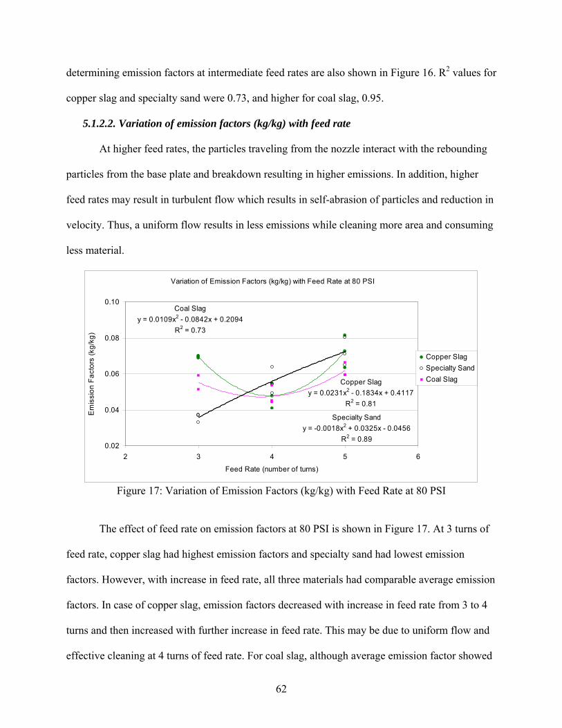
62
determining emission factors at intermediate feed rates are also shown in Figure 16. R2 values for
copper slag and specialty sand were 0.73, and higher for coal slag, 0.95.
5.1.2.2. Variation of emission factors (kg/kg) with feed rate
At higher feed rates, the particles traveling from the nozzle interact with the rebounding
particles from the base plate and breakdown resulting in higher emissions. In addition, higher
feed rates may result in turbulent flow which results in self-abrasion of particles and reduction in
velocity. Thus, a uniform flow results in less emissions while cleaning more area and consuming
less material.
Variation of Emission Factors (kg/kg) with Feed Rate at 80 PSI
Coal Slagy = 0.0109x2 - 0.0842x + 0.2094
R2 = 0.73
Copper Slagy = 0.0231x2 - 0.1834x + 0.4117
R2 = 0.81
Specialty Sandy = -0.0018x2 + 0.0325x - 0.0456
R2 = 0.890.02
0.04
0.06
0.08
0.10
2 3 4 5 6
Feed Rate (number of turns)
Em
issi
on F
acto
rs (k
g/kg
)
Copper SlagSpecialty SandCoal Slag
Figure 17: Variation of Emission Factors (kg/kg) with Feed Rate at 80 PSI
The effect of feed rate on emission factors at 80 PSI is shown in Figure 17. At 3 turns of
feed rate, copper slag had highest emission factors and specialty sand had lowest emission
factors. However, with increase in feed rate, all three materials had comparable average emission
factors. In case of copper slag, emission factors decreased with increase in feed rate from 3 to 4
turns and then increased with further increase in feed rate. This may be due to uniform flow and
effective cleaning at 4 turns of feed rate. For coal slag, although average emission factor showed

63
similar trend as copper slag, the variation was not significant. In case of specialty sand, emission
factors increased with increase in feed rate, which may be due to self-abrasion of particles and
non-uniform flow of material at higher feed rates. The regression equations for estimating
emission factors at intermediate feed rates for blast pressure of 80 PSI are also shown in Figure
17. R2 values obtained for these variations were less than 0.90.
Variation of Emission Factors (kg/kg) with Feed Rate at 100 PSI
Coal Slagy = 0.0028x2 - 0.0212x + 0.0994
R2 = 0.58
Copper Slagy = 0.0156x2 - 0.1205x + 0.2757
R2 = 0.89
Specialty Sandy = -0.0651x2 + 0.5475x - 1.0076
R2 = 0.900.00
0.04
0.08
0.12
0.16
2 3 4 5 6
Feed Rate (number of turns)
Em
issi
on F
acto
rs (k
g/kg
)
Coal SlagCopper SlagSpecialty Sand
Figure 18: Variation of Emission Factors (kg/kg) with Feed Rate at 100 PSI
Figures 18 and 19 show the variation of emission factors with feed rate at 100 and 120
PSI respectively. Coal slag showed an insignificant variation in emission factors with feed rate.
Copper slag emission factors decreased with increase in feed rate and then increased at 100 PSI
similar to the variation at 80 PSI, which may be due to more uniform flow at 4 turns. However,
at 120 PSI, this variation was not significant. This may be because of lesser effect of feed rate at
higher pressures. In case specialty sand, emission factors increased with increase in feed rate
from 3 to 4 turns and then decreased with further increase in feed rate. A more uniform flow and
less consumption of material at higher feed rates may have resulted in decreased emission factors

64
at 100 and 120 PSI. The equations to determine emission factors at intermediate feed rates for
100 and 120 PSI are also shown in Figures 18 and 19.
Variation of Emission Factors (kg/kg) with Feed Rate at 120 PSI
Coal Slagy = 0.0072x2 - 0.0554x + 0.1801
R2 = 0.92
Copper Slagy = 0.0091x2 - 0.0711x + 0.1777
R2 = 0.76
Specialty Sandy = -0.0598x2 + 0.5017x - 0.867
R2 = 0.660.00
0.04
0.08
0.12
0.16
0.20
2 3 4 5 6
Feed Rate (number of turns)
Em
issi
on F
acto
rs (k
g/kg
)
Coal SlagCopper SlagSpecialty Sand
Figure 19: Variation of Emission Factors (kg/kg) with Feed Rate at 120 PSI
5.1.2.3. Variation of emission factors (kg/kg) with pressure and feed rate
Figures 20, 21, and 22 show variation of emission factors with both pressure and feed
rate. The regression model developed to determine emission factors at intermediate pressure and
feed rate is:
)**()*()*()*()*( 22 FPfFePdFcPbaEF +++++= (3)
Where,
EF = Emission Factor in kg/kg,
P = Blast Pressure in PSI, (80 to 120 PSI),
F = Feed Rate in Number of Turns of Schmidt Feed Valve (3 to 5), and
a, b, c, d, e, and f are coefficients, given in Table 12.

65
Table 12: Coefficients for Emission Factors in (kg/kg) for Equation 3 Abrasive Material a b c d e f R2 Coal Slag 2.38E-01 -2.20E-03 -5.37E-02 1.46E-05 7.32E-03 -2.47E-05 0.94
Copper Slag 3.48E-01 -5.15E-04 -1.31E-01 8.93E-08 1.65E-02 9.52E-06 0.83Specialty Sand -7.90E-01 1.26E-03 3.49E-01 2.29E-06 -4.23E-02 1.18E-04 0.82
Figure 20: Coal Slag - Variation of Emission Factors (kg/kg) with Pressure and Feed Rate

66
Figure 21: Copper Slag - Variation of Emission Factors (kg/kg) with Pressure and Feed Rate
Figure 22: Specialty Sand - Variation of Emission Factors (kg/kg) with Pressure and Feed Rate

67
5.2. Productivity 5.1.1. Variation of Productivity with Pressure
The variation of productivity with pressure at 3, 4, and 5 turns of feed rate is shown in
Figures 23, 26, and 25, respectively. Productivity of coal slag increased with increase in pressure
at 3, 4, and 5 turns. An increase in pressure results in higher velocities and a significant increase
in the kinetic energy of abrasive particles since kinetic energy imparted to the abrasive material
is proportional to square of the velocity (V2) of the material. Thus, a greater impact is created
upon striking the plate resulting in lesser dwell time to remove paint from the surface. Hence,
productivity increased with increase in blast pressure. While this trend was observed for copper
slag and specialty sand from blast pressures 80 to 100 PSI, the productivity decreased with
further increase in pressure to 120 PSI at 3 and 4 turns. At very high pressures, the particles
undergo more damage due to self-abrasion of abrasive particles and impact of rebounding
particles causes loss of energy. Thus, kinetic energy of particles striking the plate decreases,
resulting in decreased productivity at very high pressures. In addition, worker fatigue at high
blast pressures causes decrease in productivity.
At 5 turns of feed rate, while coal slag and copper slag followed similar trends as at 3 and
4 turns, productivity of sand increased with increase in pressure. This may be due to lesser effect
of self-abrasion and rebounding particles and greater abrasive flow rate at 5 turns, which resulted
in more number of particles impacting the surface with higher kinetic energy. Specialty sand was
more effective in removing paint at a faster rate than coal slag and copper in most cases. Higher
hardness of sand grains due to improved abrasive qualities by processing from the suppliers may
have resulted in higher productivity. While coal slag and copper slag had approximately same

68
productivity at 100 PSI, coal slag resulted in higher productivity than copper slag at 80 and 120
PSI for 3, 4, and 5 turns of feed rate.
Variation of Productivity (m2/hr) with Pressure at 3 Turns
Coal Slagy = 0.0005x2 - 0.0144x + 6.3985
R2 = 0.85
Copper Slagy = -0.0087x2 + 1.7718x - 80.233
R2 = 0.98
Specialty Sandy = -0.0085x2 + 1.6955x - 70.219
R2 = 0.894.0
8.0
12.0
16.0
70 80 90 100 110 120 130
Pressure (PSI)
Pro
duct
ivity
(m2 /h
r)
Coal SlagCopper SlagSpecialty Sand
Figure 23: Variation of Productivity with Pressure at 3 Turns
Variation of Productivity (m2/hr) with Pressure at 4 Turns
Coal Slagy = 0.001x2 - 0.1252x + 16.016
R2 = 0.94
Copper Slagy = -0.0103x2 + 2.1082x - 94.018
R2 = 0.99
Specialty Sandy = -0.0094x2 + 1.9332x - 82.451
R2 = 0.955.0
10.0
15.0
20.0
70 80 90 100 110 120 130
Pressure (PSI)
Prod
uctiv
ity (m
2 /hr)
Coal SlagCopper SlagSpecialty Sand
Figure 24: Variation of Productivity with Pressure at 4 Turns
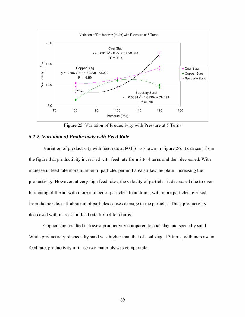
69
Variation of Productivity (m2/hr) with Pressure at 5 Turns
Coal Slagy = 0.0018x2 - 0.2708x + 20.044
R2 = 0.95
Copper Slagy = -0.0076x2 + 1.6026x - 73.203
R2 = 0.99
Specialty Sandy = 0.0091x2 - 1.6135x + 79.433
R2 = 0.985.0
10.0
15.0
20.0
70 80 90 100 110 120 130
Pressure (PSI)
Pro
duct
ivity
(m2 /h
r)
Coal SlagCopper SlagSpecialty Sand
Figure 25: Variation of Productivity with Pressure at 5 Turns
5.1.2. Variation of Productivity with Feed Rate
Variation of productivity with feed rate at 80 PSI is shown in Figure 26. It can seen from
the figure that productivity increased with feed rate from 3 to 4 turns and then decreased. With
increase in feed rate more number of particles per unit area strikes the plate, increasing the
productivity. However, at very high feed rates, the velocity of particles is decreased due to over
burdening of the air with more number of particles. In addition, with more particles released
from the nozzle, self-abrasion of particles causes damage to the particles. Thus, productivity
decreased with increase in feed rate from 4 to 5 turns.
Copper slag resulted in lowest productivity compared to coal slag and specialty sand.
While productivity of specialty sand was higher than that of coal slag at 3 turns, with increase in
feed rate, productivity of these two materials was comparable.

70
Variation of Productivity (m2/hr) with Feed Rate at 80 PSI
Coal Slagy = -3.466x2 + 28.68x - 46.583
R2 = 0.94
Copper Slagy = -2.9503x2 + 23.998x - 39.844
R2 = 0.98
Specialty Sandy = -2.096x2 + 15.717x - 17.372
R2 = 0.76
0.0
5.0
10.0
15.0
2 3 4 5 6Feed Rate (number of turns)
Prod
uctiv
ity (m
2 /hr)
Coal SlagCopper SlagSpecialty Sand
Figure 26: Variation of Productivity with Feed Rate at 80 PSI
Variation of Productivity (m2/hr) with Feed Rate at 100 PSI
Coal Slagy = -3.4479x2 + 28.399x - 44.494
R2 = 0.94
Copper Slagy = -3.8157x2 + 31.28x - 49.919
R2 = 0.995
Specialty Sandy = -4.9405x2 + 37.155x - 52.834
R2 = 0.995.0
10.0
15.0
20.0
2 3 4 5 6
Feed Rate (number of turns)
Pro
duct
ivity
(m2 /h
r)
Coal SlagCopper SlagSpecialty Sand
Figure 27: Variation of Productivity with Feed Rate at 100 PSI
Similar to variation at 80 PSI, the productivity of coal slag, copper slag, and specialty
sand at 100 PSI increased with increase in feed rate to an optimum value and then decreased with
further increase in feed rate (Figure 27). Coal slag and copper slag showed almost the same
productivity, while productivity of specialty was observed to be considerably higher from 3 to 4

71
turns. The equations to estimate productivity at intermediate feed rates are shown in also shown
in Figure 27.
The variation of productivity of three materials with feed rate at 120 PSI is shown in
Figure 28. While coal slag and copper slag showed a similar trend as previous two pressure
conditions with change in feed rate, productivity of specialty sand did not show the decreasing
trend at higher feed rates. This may be due to combined effect of higher pressure and feed rate
conditions, resulting greater velocity and higher number of particles participating in abrading
action for specialty sand compared to coal slag and copper slag. Lowest productivity was
observed for copper slag. Coal slag showed higher productivity than specialty sand at 4 turns, but
lower at 5 turns.
Variation of Productivity (m2/hr) with Feed Rate at 120 PSI
Coal Slagy = -4.238x2 + 35.209x - 56.028
R2 = 0.87Copper Slag
y = -3.0021x2 + 25.587x - 43.165R2 = 0.99
Specialty Sandy = -0.0074x2 + 3.4327x + 0.375
R2 = 0.985.0
10.0
15.0
20.0
25.0
2 3 4 5 6
Feed Rate (number of turns)
Pro
duct
ivity
(m2 /h
r)
Coal SlagCopper SlagSpecialty Sand
Figure 28: Variation of Productivity with Feed Rate at 120 PSI
5.1.3. Variation of Productivity with Pressure and Feed Rate
Figures 28, 30, and 31 show simultaneous effect of blast pressure and feed rate on
productivity for coal slag, copper slag, and specialty sand respectively.

72
Figure 29: Coal Slag - Variation of Productivity with Pressure and Feed Rate
Figure 30: Copper Slag - Variation of Productivity with Pressure and Feed Rate

73
Figure 31: Specialty Sand - Variation of Productivity with Pressure and Feed Rate
The regression model developed to determine productivity at intermediate pressure and
feed rate is:
)*/()/()/()/()/(Pr 22 FPfFePdFcPbaoductivity +++++= (4)
Where,
Productivity in m2/hr
P = Blast Pressure in PSI, (80 to 120 PSI),
F = Feed Rate in Number of Turns of Schmidt Feed Valve (3 to 5), and
a, b, c, d, e, and f are coefficients, given in Table 13.
Table 13: Coefficients for Productivity (m2/hr) for Equation 4 Abrasive Material a b c d e f R2 Coal Slag -1.85E+00 -6.33E+03 4.14E+02 2.44E+05 -8.31E+02 1.29E+03 0.94
Copper Slag -1.05E+02 1.51E+04 3.33E+02 -7.99E+05 -7.27E+02 4.03E+03 0.99Specialty Sand -2.73E+00 -1.38E+02 1.65E+02 -2.00E+05 -5.65E+02 1.33E+04 0.58

74
5.3. Consumption
5.3.1. Variation of Consumption with Pressure
The variation of abrasive consumption with pressure at 3 turns of feed rate is shown in
Figure 32. Consumption of copper slag and specialty sand decreased with increase in blast
pressure and then increased with further increase in pressure. Due to lower velocity at low
pressure, the kinetic energy possessed by the abrasive particles is less. Thus, more material was
required to remove paint and achieve desired profile. With increase in blast pressure, kinetic
energy increased, which resulted a decrease in consumption. However, at very high pressures,
particles undergo more damage at higher velocities due to self-abrasion., which resulted in
increased consumption for coal slag and copper slag.
Variation of Consumption (kg/m2) with Pressure at 3 Turns
Coal Slagy = -0.004x2 + 0.9377x - 15.043
R2 = 0.73
Copper Slagy = 0.0293x2 - 5.4216x + 285.05
R2 = 0.98
Specialty Sandy = 0.0133x2 - 2.7635x + 167.62
R2 = 0.4615.0
30.0
45.0
60.0
70 80 90 100 110 120 130
Pressure (PSI)
Con
sum
ptio
n (k
g/m
2 )
Coal SlagCopper SlagSpecialty Sand
Figure 32: Variation of Consumption with Pressure at 3 Turns
Although an increase in consumption of specialty sand was observed with increase
pressure from 100 to 120 PSI, the variation was not significant. Minimum consumption of
material was observed in case of specialty sand at 3 turns. While coal slag and copper slag

75
consumed comparable quantities of material from 80 to 100 PSI, at higher pressure, copper slag
showed a significant increase in consumption. This may be due to greater damage of particles for
copper slag compared to coal slag. R2 value obtained for specialty sand was considerably lower
than the values for coal slag and copper slag at 3 turns.
Variation of Consumption (kg/m2) with Pressure at 4 Turns
Coal Slagy = -0.013x2 + 2.607x - 97.174
R2 = 0.63
Copper Slagy = -0.0004x2 - 0.1288x + 57.205
R2 = 0.46
Specialty Sandy = 0.009x2 - 1.8871x + 119.61
R2 = 0.7715.0
30.0
45.0
60.0
70 80 90 100 110 120 130
Pressure (PSI)
Con
sum
ptio
n (k
g/m
2 )
Coal SlagCopper SlagSpecialty Sand
Figure 33: Variation of Consumption with Pressure at 4 Turns
Figure 33 shows the variation of consumption with pressure at 4 turns. It can be observed
from the figure that effect of pressure on consumption was not significant in case of all three
materials, which may be due to more uniform flow of material at turns. However, consumption
of copper slag was higher than coal slag and specialty sand. Minimum material was consumed in
case of specialty sand. The equations to determine material consumption for coal slag, copper
slag, and specialty sand are shown in Figure 33 and lower R2 values (<0.80) were obtained for all
three materials.
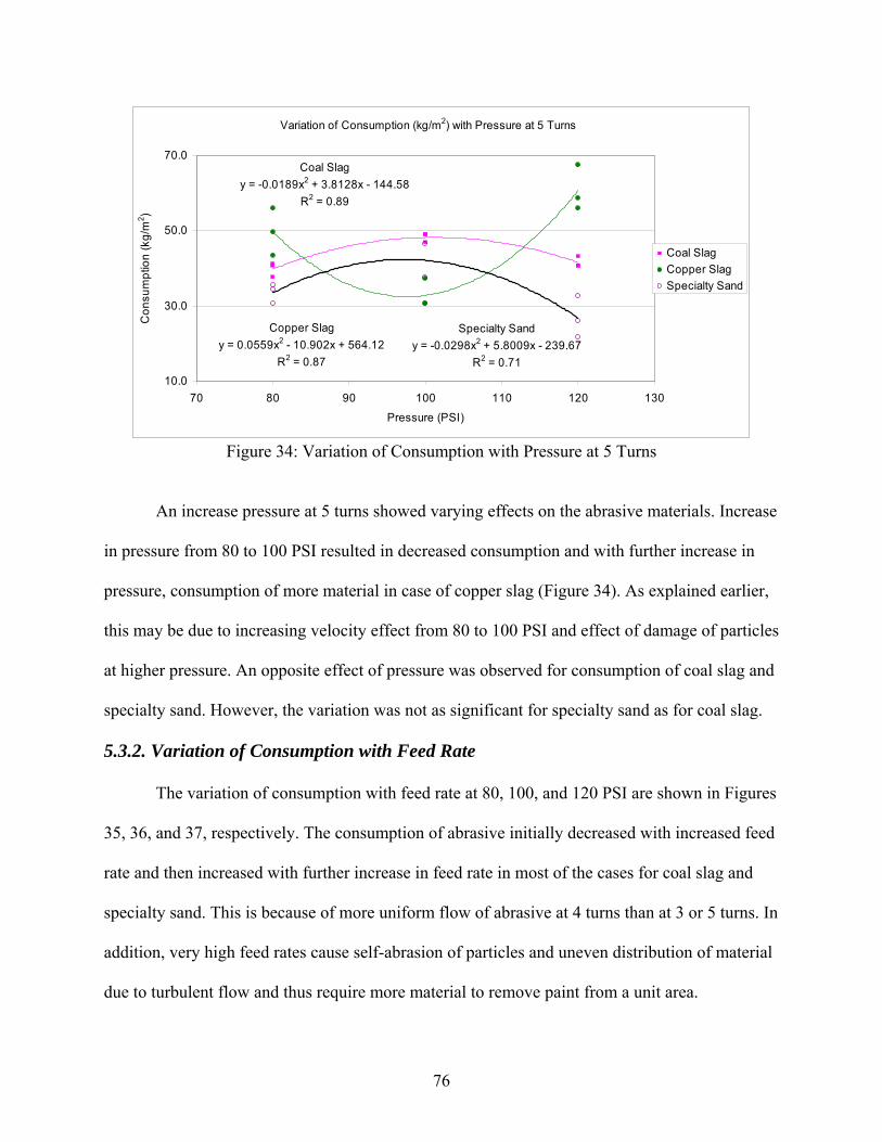
76
Variation of Consumption (kg/m2) with Pressure at 5 Turns
Coal Slagy = -0.0189x2 + 3.8128x - 144.58
R2 = 0.89
Copper Slagy = 0.0559x2 - 10.902x + 564.12
R2 = 0.87
Specialty Sandy = -0.0298x2 + 5.8009x - 239.67
R2 = 0.7110.0
30.0
50.0
70.0
70 80 90 100 110 120 130
Pressure (PSI)
Con
sum
ptio
n (k
g/m
2 )
Coal SlagCopper SlagSpecialty Sand
Figure 34: Variation of Consumption with Pressure at 5 Turns
An increase pressure at 5 turns showed varying effects on the abrasive materials. Increase
in pressure from 80 to 100 PSI resulted in decreased consumption and with further increase in
pressure, consumption of more material in case of copper slag (Figure 34). As explained earlier,
this may be due to increasing velocity effect from 80 to 100 PSI and effect of damage of particles
at higher pressure. An opposite effect of pressure was observed for consumption of coal slag and
specialty sand. However, the variation was not as significant for specialty sand as for coal slag.
5.3.2. Variation of Consumption with Feed Rate
The variation of consumption with feed rate at 80, 100, and 120 PSI are shown in Figures
35, 36, and 37, respectively. The consumption of abrasive initially decreased with increased feed
rate and then increased with further increase in feed rate in most of the cases for coal slag and
specialty sand. This is because of more uniform flow of abrasive at 4 turns than at 3 or 5 turns. In
addition, very high feed rates cause self-abrasion of particles and uneven distribution of material
due to turbulent flow and thus require more material to remove paint from a unit area.
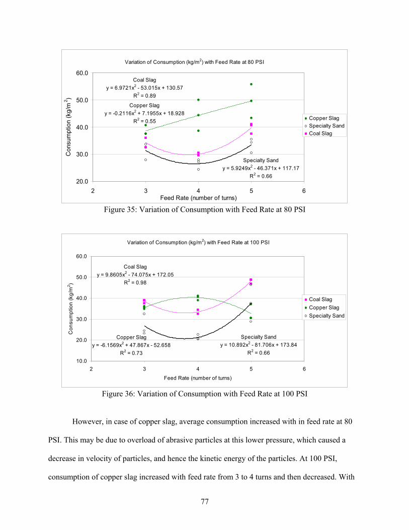
77
Variation of Consumption (kg/m2) with Feed Rate at 80 PSI
Coal Slagy = 6.9721x2 - 53.015x + 130.57
R2 = 0.89
Copper Slagy = -0.2116x2 + 7.1955x + 18.928
R2 = 0.55
Specialty Sandy = 5.9249x2 - 46.371x + 117.17
R2 = 0.6620.0
30.0
40.0
50.0
60.0
2 3 4 5 6Feed Rate (number of turns)
Con
sum
ptio
n (k
g/m
2 )
Copper SlagSpecialty SandCoal Slag
Figure 35: Variation of Consumption with Feed Rate at 80 PSI
Variation of Consumption (kg/m2) with Feed Rate at 100 PSI
Coal Slagy = 9.8605x2 - 74.075x + 172.05
R2 = 0.98
Copper Slagy = -6.1569x2 + 47.867x - 52.658
R2 = 0.73
Specialty Sandy = 10.892x2 - 81.706x + 173.84
R2 = 0.6610.0
20.0
30.0
40.0
50.0
60.0
2 3 4 5 6
Feed Rate (number of turns)
Con
sum
ptio
n (k
g/m
2 )
Coal SlagCopper SlagSpecialty Sand
Figure 36: Variation of Consumption with Feed Rate at 100 PSI
However, in case of copper slag, average consumption increased with in feed rate at 80
PSI. This may be due to overload of abrasive particles at this lower pressure, which caused a
decrease in velocity of particles, and hence the kinetic energy of the particles. At 100 PSI,
consumption of copper slag increased with feed rate from 3 to 4 turns and then decreased. With

78
increase in feed rate, more number of particles participated in abrading action per unit area,
which may have resulted in decrease of consumption at higher feed rate for 100 PSI.
Variation of Consumption (kg/m2) with Feed Rate at 120 PSI
Coal Slagy = 12.122x2 - 96.052x + 218.71
R2 = 0.97
Copper Slagy = 19.751x2 - 153.11x + 332.39
R2 = 0.77
Specialty Sandy = 3.3869x2 - 29.755x + 90.87
R2 = 0.160.0
20.0
40.0
60.0
80.0
2 3 4 5 6
Feed Rate (number of turns)
Con
sum
ptio
n (k
g/m
2 )
Coal SlagCopper SlagSpecialty Sand
Figure 37: Variation of Consumption with Feed Rate at 120 PSI
Copper slag resulted in higher consumption than coal slag and specialty sand at 80 and
120 PSI. While minimum consumption was observed for specialty sand at 80 and 120 PSI, the
consumption of abrasives demonstrated a mixed effect at 100 PSI for the three materials. The
equations and R2 values obtained from regression analysis for these variations are shown in the
figures above.
5.3.3. Variation of Consumption with Pressure and Feed Rate
The variation of consumption with both pressure and feed rate for coal slag, copper slag,
and specialty sand are shown in Figures 38, 39, and 40.
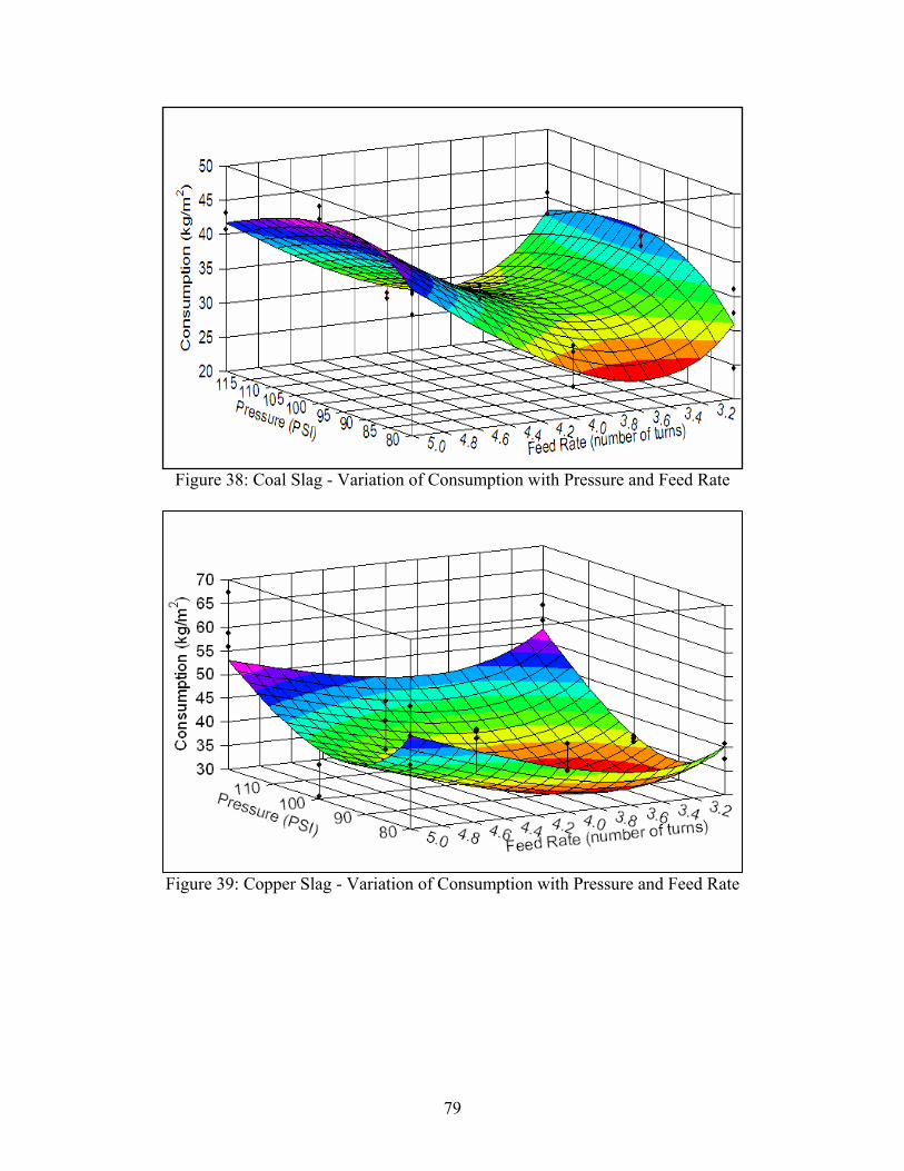
79
Figure 38: Coal Slag - Variation of Consumption with Pressure and Feed Rate
Figure 39: Copper Slag - Variation of Consumption with Pressure and Feed Rate

80
Figure 40: Specialty Sand - Variation of Consumption with Pressure and Feed Rate
The regression model developed to determine consumption at intermediate pressure and
feed rate is:
)*/()/()/()/()/( 22 FPfFePdFcPbanConsumptio +++++= (5)
Where,
Consumption in kg/m2
P = Blast Pressure in PSI, (80 to 120 PSI),
F = Feed Rate in Number of Turns of Schmidt Feed Valve (3 to 5), and
a, b, c, d, e, and f are coefficients, given in Table 14.
Table 14: Coefficients for Consumption (kg/m2) for Equation 5
Abrasive Material a b c d e f R2 Coal Slag 7.13E+01 2.73E+04 -1.27E+03 -1.20E+06 2.54E+03 -1.26E+04 0.86
Copper Slag 4.25E+02 -5.38E+04 -7.55E+02 2.70E+06 1.66E+03 -1.61E+04 0.51Specialty Sand 1.34E+02 -7.91E+01 -8.25E+02 1.47E+05 1.69E+03 -9.43E+03 0.30
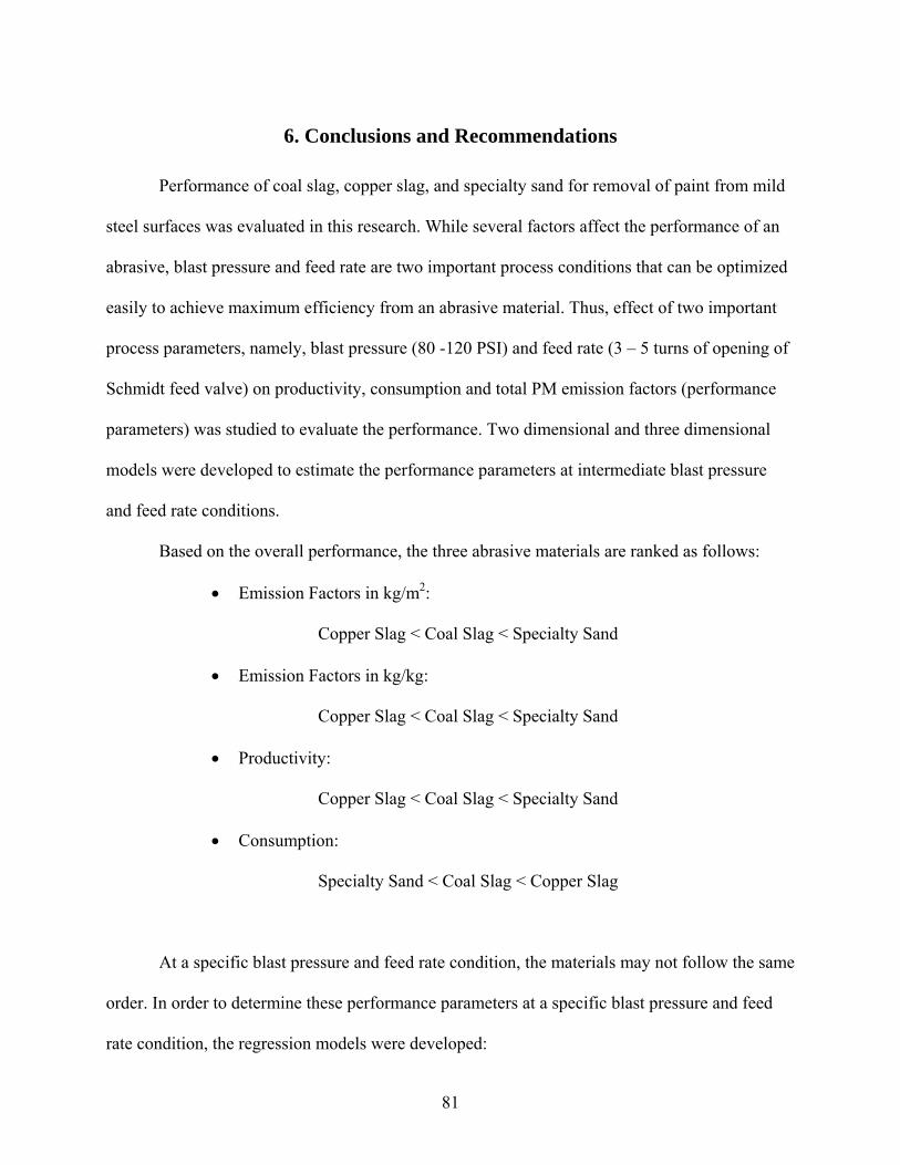
81
6. Conclusions and Recommendations
Performance of coal slag, copper slag, and specialty sand for removal of paint from mild
steel surfaces was evaluated in this research. While several factors affect the performance of an
abrasive, blast pressure and feed rate are two important process conditions that can be optimized
easily to achieve maximum efficiency from an abrasive material. Thus, effect of two important
process parameters, namely, blast pressure (80 -120 PSI) and feed rate (3 – 5 turns of opening of
Schmidt feed valve) on productivity, consumption and total PM emission factors (performance
parameters) was studied to evaluate the performance. Two dimensional and three dimensional
models were developed to estimate the performance parameters at intermediate blast pressure
and feed rate conditions.
Based on the overall performance, the three abrasive materials are ranked as follows:
• Emission Factors in kg/m2:
Copper Slag < Coal Slag < Specialty Sand
• Emission Factors in kg/kg:
Copper Slag < Coal Slag < Specialty Sand
• Productivity:
Copper Slag < Coal Slag < Specialty Sand
• Consumption:
Specialty Sand < Coal Slag < Copper Slag
At a specific blast pressure and feed rate condition, the materials may not follow the same
order. In order to determine these performance parameters at a specific blast pressure and feed
rate condition, the regression models were developed:

82
)**()*()*()*()*( 22 FPfFePdFcPbaEF +++++= )*/()/()/()/()/( 22 FPfFePdFcPbaY +++++=
Where,
EF = Emission Factor in kg/m2 or kg/kg
Y = Productivity in m2/hr or Consumption in kg/m2
P = Blast Pressure in PSI, (80 to 120 PSI)
F = Feed Rate in Number of Turns of Schmidt Feed Valve (3 to 5)
a, b, c, d, e, and f are coefficients, which vary for each material and performance
parameter.
Due caution must be employed while using these equations. The results are valid within
the tested ranges of blast pressure and feed rate.
Emission quantities and health risk can be estimated using the emission factors developed
in this research. Spent abrasive quantities can be estimated by estimating the quantity of abrasive
used from the consumption models developed in this research. With additional information on
specific costs, emission factors, productivity and consumption models can be used to determine
material costs, labor costs, equipment costs, energy costs, emission control & compliance costs,
waste disposal costs, and health risk costs. An example of application of these equations in cost
calculations is shown in Appendix D.
It is evident from the above results that specialty sand is cost-effective with respect to
production costs due to highest productivity and lowest consumption. However, it also has
highest emission potential, which increases emission control and compliance costs, health risk to
workers. Moreover, emissions from sand are of great concern due to silicosis caused by silica
83
emissions and many health and regulatory agencies require the use of substitute materials to
reduce the risk of silicosis.
While coal slag has higher emission factors than copper slag, overall life cycle costs may
be lower than copper slag because of higher productivity and lower consumption of coal slag.
With increasing concern on environmental and health effects due to PM emissions, it is
important to evaluate pollution prevention, cost reduction options and health risk of alternative
materials prior to selecting an abrasive.
Size distribution and metal analysis of total PM emissions will greatly enhance the health
risk evaluation due to metal and particulate emissions. This research was focused on effect of
blast pressure and feed rate on performance of medium grade, non-reusable abrasives. It is
recommended to study the effect of other parameters such as nozzle size, and abrasive grade on
the performance.
The exhaust flow rate is important when emissions are estimated. With higher flow rate,
more particles get airborne due to higher suction in the test chamber. Thus, emission factors may
be higher. Effect of exhaust flow rate on emission factors may be studied in future research.
Since thickness of surface contamination affects the performance of an abrasive, effect of
varying paint thickness may be studied.
Since the blasting operations were carried in an enclosed chamber emission factors
developed in this research must be extrapolated for other sizes of blast chambers and open-air
blasting due to effect of wind velocity in case of outdoor blasting.

84
References
Abrasive Blasting, 1995. Industry Code of Practice, Workplace Health and Safety Act 1995, Queensland, Australia. Angie M.O. and Wayne G. L., 1999. Assessment of Environmental Toxicity from Spent Recycled Glass Abrasives Part A. Data Review. Institute of Environmental Toxicology and Chemistry. Western Washington University, Washington. Appleman, B.R., Weaver, R.E., Boocock, S.K., 1998. Users’ Guide To Selecting Abrasives. Journal of Protective Coating & Linings, pp 89-99. Atkinson, R.W., Anderson, H.R., Sunyer, J., Ayres, J., Baccini, M., Vonk, J.M., Boumghar, A., Forastiere, F., Forsberg, B., Touloumi, G., Schwartz, J., and Katsouyanni, K., 2001. ‘Acute Effects of Particulate Air Pollution on Respiratory Admissions. Results from APHEA 2 Project’, Am. J. Respir. Crit. Care Med., Vol. 164, Number 10, pp. 1860-1866. BAAQMD, 1990. Sandblasting, Miscellaneous Standards for Performance, Regulation 12, Rule 2, Bay Area Air Quality Management District, CA. BAAQMD, 1998. Abrasive Blasting (Confined), Bay Area Air Quality Management District Permit Handbook, Bay Area Air Quality Management District, CA. Clemco Industries, Inc.,1989. “Achieving Productivity from Abrasive Blast Cleaning Systems.” Journal of Protective Coatings & Linings, 9, pp 31-36. Conroy, L.M.; Menezes-Lindsay, R.M.; Sullivan, P.M.; Cali, S.; Forst, L. Lead, chromium, and cadmium exposure during abrasive blasting. Arch. Environ. Health 1996, 51(2), 95–99. Daigle, C.C; Chalupa, D.C.; Gibb, F.R.; Morrow, P.E.; Oberdorster, G.; Utell, M.J.; Frampton, M.W., 2003 Ultrafine Particle Deposition in Humans During Rest and Exercise. Inhalation Toxicology. Datar, S.R., 2003. Environmental Performance of Coal Slag and Garnet as Abrasives. A Thesis. University of New Orleans, New Orleans, LA. Dockery, D.W.; Pope, C.A.; Xu, X.; Spengler, J.D.; Ware, J.H.; Fay, M.E.; Ferris, B.G.; and Speizer, F.E., 1993. ‘An Association between Air Pollution and Mortality in Six U.S. Cities’, N. Engl. J. Med., 329(24), pp 1753-1759. McBean, E.A., and Rovers, F.A., 1998. Statistical Procedures for Analysis of Environmental Monitoring Data & Risk Assessement. Volume 3, Prentice Hall PTR, Upper Saddle River, NJ 07458.

85
Hansink, J.D., 1995. Minimizing dust during abrasive blast cleaning. Journal of Protective Coating & Linings , 12 (4), pp 18-19. Hansink, J.D., 2000. An Introduction to Abrasives for Protective Coating Removal Operations. Journal of Protective Coating & Linings, pp 66-73. Holt W.S; Austin, D.M., 2001. How Nozzle Pressure and Feed Rate Affect the Productivity of Dry Abrasive Blasting. Journal of Protective Coatings & Linings, pp 82-104. Hubbs, A.F.; Minhas, N.S.; Jones, W.; Greskevitch, M.; Battelli, L.A.; Porter, D.W.; Goldsmith,W. T.; Frazer, D.; Landsittel, D. P.; Ma, J. Y. C.; Barger, M.; Hill, K.; Schwegler-Berry, D.; Robinson, V. A.; Castranova, V., 2001. Comparative Pulmonary Toxicity of 6 Abrasive Blasting Agents. Toxicol. Science, 61, pp 135-143. JPCL, 2000. NSRP Studies Minimizing Waste from Mineral Slags, Journal of Protective Coatings & Linings, pp 73-77. Kleinbaum, D.G., Kupper, L.L., Muller, K.E., 1992. Applied Regression Analysis and Other Multivariate Methods, Second Edition, PWS-KENT Publishing Company. LDEQ, 1998. Abrasive Blasting, Louisiana Department of Environmental Quality, LA. Available at: http://www.deq.state.la.us/assistance/sbap/regs/abrasive.htm (accessed on 03/10/05). Lipton, D.M., and R.L. Herring, 1996. Respirable crystalline silica dust exposure during abrasive blast cleaning of bridge deck surfaces. Appl. Occup. Environ. Hyg. 11, pp 81–83. MacKay, G.R.; Stettler, L.E.; Kommineni, C.; Donaldson H.J. Fibrogenic potential of slags used as substitutes for sand in abrasive blasting operations. Am. Ind. Hyg. Assoc. J. 1980, 41(11), pp 836–842. National Steel and Shipbuilding Company, 1999. Feasibility and Economics Study of the Treatment, Recycling and Disposal of Spent Abrasives (Document Number: NSRP-0529). NAVFAC, 1998. Recycling Spent Sandblasting Grit and Similar Wastes as Aggregate in Asphaltic Concrete. TDS-2065-ENV, Naval Facilities Engineering Service Center, Port Hueneme, CA. NFESC, 1996. Recycling and Reuse Options for Spent Abrasive Blasting Media and Similar Wastes. TM-2178-ENV, Naval Facilities Engineering Service Center, Port Hueneme, CA. NIOSH, 1974. Abrasive Blasting Respiratory Protective Practices, National Institute for Occupational Safety and Health, Pub. No.74-104., Cincinnati, Ohio. NIOSH, 1998. Evaluation of Substitute Materials for Silica Sand in Abrasive Blasting. National Institute for Occupational Safety and Health.
86
NIOSH, 2001. Nomination of Abrasive Blasting Agents for Chronic Inhalation Studies in Rats. National Institute for Occupational Safety and Health. NSRP, 1999. Particulate Emission Factors for Blasting Operations and Other Potential Sources. NSRP 0552, N1-97-4. National Shipbuilding Research Program. Oberdorster, G., 1995. Lung particle overload: implications for occupational exposures to particles, Reg. Toxicol. Pharmacol. Obery, A.M., Wayne, G.L., 1999. Assessment of Environmental Toxicity from Spent Recycled Glass Abrasives Part A. Data Review. Institute of Environmental Toxicology and Chemistry. Western Washington University, Washington. Paddison, R.D., 2000. “What Type of Abrasive to Use? An Overview on Selection and Use of Common Blast-Cleaning Materials.” Protective Coatings Europe, 5, pp 10-16. PCRC. Mechanical Coatings Removal: Regulatory Requirements. EPA Self-Audit and Inspection Guide Organic Finishing of Metals, Paints and Coatings Resource Center. Available at: http://www.paintcenter.org/ctc/Mechrem2.cfm (accessed: 06/03/2005). Pope, C.A.; Bates, D.; Raizenne, M., 1995. Health effects of particulate air pollution: Time for reassessment. Environ. Health Perspect., 103, pp 472-480. Rappaport, S.M., Goldberg, M., Susi, P., and Herrick, R.F., 2003. Excessive exposure to silica in the U.S. construction industry. Ann. Occup. Hyg. 47, pp 111–122. Reed Minerals. Available at: http://www.reedmin.com/products/abrasives.html (accessed on: 01/10/05). SCAQMD, 1989. Unconfined Abrasive Blasting, South Coast Air Quality Management District Permit Processing Handbook, Section 2, South Coast Air Quality Management District, CA. Schwartz, J., 2004 ‘The effects of particulate air pollution on daily deaths: a multi-city case crossover analysis’ Occupational and Environmental Medicine, Vol. 61, pp. 956-961. SDAPCD, Abrasive Blasting Procedures, Emission Factors, The County of San Diego Air Pollution Control District, CA. Available at: http://www.sdapcd.org/toxics/emissions/ablast/ablast.html (accessed on: 03/10/05). Seavey, M., 1985. Abrasive Blasting above 100 psi. Journal of Protective Coating & Linings, pp 26- 37. Silvadasan, X., 2004. Environmental Performance of Steel Grit and Specialty Sand as Abrasives. A Thesis. University of New Orleans, New Orleans, LA.

87
SSPC. Surface Preparation Standards and Specifications, the Society of Protective Coatings. Available at: http://www.sspc.org/standards/scopes.html#sp (accessed on: 03/02/05). Technology Publishing Company, 1999. Techniques of Air Abrasive Blasting, APPLICATOR TRAINING BULLETIN, Protective Coatings Europe, pp 52-53. TNRCC, 1993. Table 27, Abrasive Blast Cleaning, Office of Permitting, Remediation and Registration, Air Permits Division, Texas Natural Resource Conservation Commission, TX. TNRCC, 2001. Abrasive Blast Cleaning, Air Permits Division, Texas Natural Resource Conservation Commission, TX. Townsend, T.G., 1997. “Disposal and Reuse Options for Used Sandblasting Grit.” Florida Center for Solid and Hazardous Waste Management. U.S. ACE, 1995. Painting: New Construction and Maintenance, Chapter 7. Surface Preparation. EM 1110-2-3400. U.S. Army Corps of Engineers, pp 4-15. U.S. EPA. Health and Environmental Impacts of PM. Office of Air Quality Planning and Standards, U.S. Environmental Protection Agency. Available at: http://www.epa.gov/air/urbanair/pm/hlth1.html (accessed: 03/01/05). U.S. EPA, 1994. Waste Prevention WasteWi$e Tip Sheet, EPA530-F-94-003, Solid Waste and Emergency Response, U.S. Environmental Protection Agency. U.S. EPA, 1997a. Emission Factor Documentation for AP-42, Section 13.2.6, Abrasive Blasting, Final Report, EPA Contract 68-D2-0159, MRI Project No. 4604-02, Office of Air Quality Planning and Standards, U.S. Environmental Protection Agency, pp 33-34. U.S. EPA, 1997b. Profile of the Shipbuilding and Ship Repair Industry, EPA Office of Compliance Sector Notebook Project, EPA/310-R-97-008, Office of Compliance, Office of Enforcement and Compliance Assurance, U.S. Environmental Protection Agency. U.S. EPA, 1997c. Procedures for Preparing Emission Factor Documents, EPA-454/R-95-015, Revised, Office of Air Quality Planning and Standards, Office of Air and Radiation, U.S. Environmental Protection Agency. U.S. EPA, 1997d. ‘Method 1: Sample and velocity traverses for stationary sources’, 40 CFR Part 60, Appendix A, Emissions Measurement Center, U.S. Environmental Protection Agency. U.S. EPA, 1997e. ‘Method 2: Determination of Stack Gas Velocity and Volumetric Flow Rate (Type S Pitot Tube)’, 40 CFR Part 60, Appendix A, Emissions Measurement Center, U.S. Environmental Protection Agency. U.S. EPA, 1997f. ‘Method 4: Determination of Moisture Content in Stack Gases’, 40 CFR Part 60, Appendix A, Emissions Measurement Center, U.S. Environmental Protection Agency.

88
U.S. EPA, 1997g. ‘Method 5: Determination of Particulate Matter Emissions from Stationary Sources’, 40 CFR Part 60, Appendix A, Emissions Measurement Center, U.S. Environmental Protection Agency. U.S. EPA, 2001. Environmentally Preferable Purchasing. EPA530-N-01-002, Solid Waste and Emergency Response, U.S. Environmental Protection Agency. U.S. EPA, 2003. ‘Particulate Pollution and Your Health’, EPA-452/F-03-001, Office of Air and Radiation, U.S. . Environmental Protection Agency, NC. U.S. EPA, 2004a. Particulate Matter Research Program, Five Years of Progress. EPA 600/R-04/058. U.S. Environmental Protection Agency. U.S. EPA, 2004b. Air Quality Criteria for Particulate Matter. National Center for Environmental Assessment: Research Triangle Park, NC, U.S. Environmental Protection Agency. Vallyathan, V.; Blake, T.; Leonard, S.; Greskevitch, M.; Jones, W.; Pack, D., 1999. In vitro toxicity of silica substitutes used for abrasive blasting. Am. J. Ind. Med. Suppl., 1, pp 158–160. Virginia Materials Inc. Available at: http://www.optaminerals.com/blackblast.html (accessed on: 01/8/05). Voutilainen. A.; Kaipio, J.P.; Pekkanen, J.; Timonen, K.L.; Ruuskanen. J., 2004 Theoretical analysis of the influence of aerosol size distribution and physical activity on particle deposition pattern in human lungs. Scandinavian J. Work, Environ & Health. Wilson Jr, F. J.; Hiller, F. C.; Wilson, J. D.; Bone, R. C., 1985. Quantitative Deposition of Ultrafine Stable Particles in the Human Respiratory Tract. Journal of Applied Physiology.

89
APPENDIX A: Field Observations and Stack Calculations

90
Table: Coal Slag: CO 120-4-1 Field Observations Date 6/14/2004 Type of Abrasive = Coal Slag Mass of Abrasive = 100 lbs Area Cleaned = 17 sqft Blast Time = 5 mins
Finish = Near
White Abrasive Grade = Medium K factor = 1.13 Blast Pressure = 120 psi Run No = 1 Abrasive feed rate = 4 # turns of on Schmidt valve Initial meter reading = 161.81
Stack Temp Vacuum Traverse
Pt Meter
Reading Delta P Delta H DGM in DGM Out
Avg Meter Temp (oF) oC oF
Hot Box Temp (oF)
Cold Box Temp (oF)
1 162.51 0.37 0.418 107 105 106 27 80.6 3 190 50 2 163.18 0.39 0.440 106 104 105 27 80.6 3 210 48 3 163.86 0.38 0.429 104 102 103 26 78.8 3 210 48 4 164.51 0.38 0.429 104 102 103 26 78.8 3 205 48 5 166.28 0.6 0.677 103 101 102 26 78.8 3 200 46 6 168.15 0.61 0.688 103 101 102 26 78.8 4 190 44 7 169.17 1.1 1.241 103 101 102 26 78.8 5 175 45 8 170.02 0.99 1.117 103 102 102.5 26.5 79.7 5 165 45
V dgm = 8.21
Average = 0.603 0.680 Avg
Temp = 103.1875 79.3625
Impinger Data Impinger
1 Impinger
2 Impinger
3 Impinger
4 Particulate Mass Collected
(Silica Gel) Filter Beaker
Final 530 549 433.5 544.5 Initial Mass (g) 0.8242 112.7509 Initial 528 548 433.5 543 Final mass (g) 0.8298 113.5333
Mass Collected 0.0056 0.7824 Difference 2 1 0 1.5 Total 0.7880 g
Volume of Water Condensed, Vwc 3 ml
Mass increase in Silica gel, (mf-mi) 1.5 g

91
Symbol Description Comments Units Value V1 Initial Meter Reading dcf 161.810 V2 Final Meter Reading dcf 170.020
Vm Actual Volume of gas measured by the DGM (Final-Initial) meter reading dcf 8.210
Tstd Standard Temperature 25oC = 298oK R 536.690
Conversion factor (in.of Hg to mm.of Hg) 25.400
Y Y(DGM correction factor: 0.95-1.05) 0.990
PB Barometric Pressure Assumed to be 30.06 in Hg 30.060 ∆ P Average ∆ P in. H20 0.603
= 0.763/13.6 in Hg 0.044 Pstd Standard Pressure in Hg 29.920 ∆ H@ Reference ∆ H From DGM Calibration in. H20 1.80
K K Factor for ∆ H Assuming Pdgm ~ Pbar 1.13 ∆ H Average ∆ H K*∆ P in. H20 0.68
Pdgm Pressyre of the DGM PB + (∆ P/13.6) in Hg 30.104 Tdgm Temperature of the DGM F 103.188
R 562.878
Vdgm(std) Volume of gas at standard conditions
Vdgm*Y*(Pdgm*Tstd) (Pstd*Tdgm)
SCF 7.797
Vwc Volume of water vapor condensed From Impingers 1, 2, & 3 ml 3.000
Vwc(std) Volume of water vapour at Standard Conditions K1*(Vw) where K1=0.04707 0.141
mf - mi Mass increase in Silica Gel From Impinger 4 g 1.500
Vwsg(std) Volume of vapor absorbed onto the silica gel K2*(mf - mi) where K2=0.04715 ml 0.071
BH2O Mole fraction of dry gas
[Vwc(std) + Vwsg(std)] X 100 [Vwc(std) + Vwsg(std) + Vdgm(std)] % 2.646
PMOS 0.974 Mdry Molecular Weight Dry Gas Assumed to be 28.6 28.600
Mgas Total Molecular Weight of Gas
Mgas = Mdry X (1-BH2O) + (18 X BH2O) 28.320
DPS √(∆P) in H20 0.776 TS Average Stack Temp DEG F 79.363 R 539.053
PS Stack Pressure Absolute (Pstat) PB + (∆ H/13.6) in Hg 30.109
Cp Pitot Tube Coeff 0.840
VS Average Stack Gas Velocity Kp * Cp* sqrt(Tgas*∆ P/(Pstat
*Mgas) where Kp = 85.49* 60 fpm 2659.199 Dia(stack) Inside Diameter of Stack in 12.000
AS Stack Area(sq.in) sq in. 113.097 AS Stack Area(sq ft) sq.ft 0.785
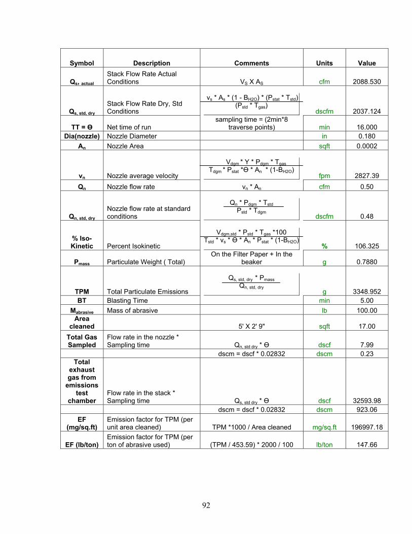
92
Symbol Description Comments Units Value
Qs, actual Stack Flow Rate Actual Conditions VS X AS cfm 2088.530
Qs, std, dry Stack Flow Rate Dry, Std Conditions
vs * As * (1 - BH2O) * (Pstat * Tstd)
(Pstd * Tgas) dscfm 2037.124
TT = Ө Net time of run sampling time = (2min*8
traverse points) min 16.000 Dia(nozzle) Nozzle Diameter in 0.180
An Nozzle Area sqft 0.0002
vn Nozzle average velocity
Vdgm * Y * Pdgm * Tgas
Tdgm * Pstat *Ө * An * (1-BH2O) fpm 2827.39
Qn Nozzle flow rate vn * An cfm 0.50
Qn, std, dry Nozzle flow rate at standard conditions
Qn * Pdgm * Tstd
Pstd * Tdgm dscfm 0.48
% Iso-Kinetic Percent Isokinetic
Vdgm,std * Pstd * Tgas *100
Tstd * vs * Ө * An * Pstat * (1-BH2O) % 106.325
Pmass Particulate Weight ( Total) On the Filter Paper + In the
beaker g 0.7880
TPM Total Particulate Emissions
Qs, std, dry * Pmass
Qn, std, dry g 3348.952
BT Blasting Time min 5.00 Mabrasive Mass of abrasive lb 100.00
Area cleaned 5' X 2' 9" sqft 17.00
Total Gas Sampled
Flow rate in the nozzle * Sampling time Qn, std dry * Ө dscf 7.99
dscm = dscf * 0.02832 dscm 0.23 Total
exhaust gas from
emissions test
chamber Flow rate in the stack * Sampling time Qs, std dry * Ө dscf 32593.98
dscm = dscf * 0.02832 dscm 923.06 EF
(mg/sq.ft) Emission factor for TPM (per unit area cleaned) TPM *1000 / Area cleaned mg/sq.ft 196997.18
EF (lb/ton) Emission factor for TPM (per ton of abrasive used) (TPM / 453.59) * 2000 / 100 lb/ton 147.66

93
APPENDIX B: Results of Statistical Analysis
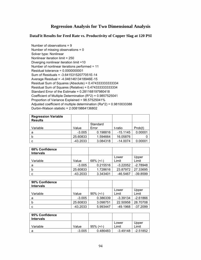
94
Regression Analysis for Two Dimensional Analysis DataFit Results for Feed Rate vs. Productivity of Copper Slag at 120 PSI Number of observations = 9 Number of missing observations = 0 Solver type: Nonlinear Nonlinear iteration limit = 250 Diverging nonlinear iteration limit =10 Number of nonlinear iterations performed = 11 Residual tolerance = 0.0000000001 Sum of Residuals = -3.64153152077051E-14 Average Residual = -4.04614613418946E-15 Residual Sum of Squares (Absolute) = 0.474333333333334 Residual Sum of Squares (Relative) = 0.474333333333334 Standard Error of the Estimate = 0.281168197980418 Coefficient of Multiple Determination (R^2) = 0.9857525041 Proportion of Variance Explained = 98.57525041% Adjusted coefficient of multiple determination (Ra^2) = 0.9810033388 Durbin-Watson statistic = 2.00819864136802 Regression Variable Results
Variable Value Standard Error t-ratio Prob(t)
a -3.005 0.198816 -15.1145 0.00001 b 25.60833 1.594664 16.05876 0 c -43.2033 3.084318 -14.0074 0.00001 68% Confidence Intervals
Variable Value 68% (+/-) Lower Limit
Upper Limit
a -3.005 0.215516 -3.22052 -2.78948 b 25.60833 1.728616 23.87972 27.33695 c -43.2033 3.343401 -46.5467 -39.8599 90% Confidence Intervals
Variable Value 90% (+/-) Lower Limit
Upper Limit
a -3.005 0.386339 -3.39134 -2.61866 b 25.60833 3.098751 22.50958 28.70708 c -43.2033 5.993447 -49.1968 -37.2099 95% Confidence Intervals
Variable Value 95% (+/-) Lower Limit
Upper Limit
a -3.005 0.486483 -3.49148 -2.51852

95
b 25.60833 3.901984 21.70635 29.51032 c -43.2033 7.547018 -50.7504 -35.6563 99% Confidence Intervals
Variable Value 99% (+/-) Lower Limit
Upper Limit
a -3.005 0.73709 -3.74209 -2.26791 b 25.60833 5.912058 19.69628 31.52039 c -43.2033 11.4348 -54.6381 -31.7685 Variance Analysis
Source DF Sum of Squares
Mean Square F Ratio Prob(F)
Regression 2 32.81807 16.40903 207.5633 0Error 6 0.474333 7.91E-02 Total 8 33.2924

96
Residuals for Two Dimensional Analyses for Feed Rate vs. Productivity of Copper Slag
Feed Rate
(No. of turns)
Observed Productivity
(m2/hr) Predicted
Productivity Residual % Error Absolute Residual
Min. Residual
Max. Residual
3 6.77 6.576666667 0.193333 2.855736 0.193333 -0.42333 0.3866673 6.27 6.576666667 -0.30667 -4.89102 0.306667 3 6.69 6.576666667 0.113333 1.694071 0.113333
4 11.15 11.15-5.33E-
15-4.78E-
14 5.33E-15
4 11.15 11.15-5.33E-
15-4.78E-
14 5.33E-15
4 11.15 11.15-5.33E-
15-4.78E-
14 5.33E-15 5 9.29 9.713333333 -0.42333 -4.55687 0.423333 5 9.75 9.713333333 0.036667 0.376068 0.036667 5 10.1 9.713333333 0.386667 3.828383 0.386667
Residual Scatter Diagram
Residual Scatter Diagram
-0.5
-0.4
-0.3
-0.2
-0.1
0
0.1
0.2
0.3
0.4
0.5
4 5 6 7 8 9 10 11 12
Predicted Productivity
Res
idua
l
Residual
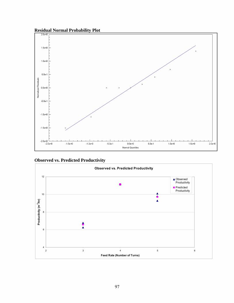
97
Residual Normal Probability Plot
Observed vs. Predicted Productivity
Observed vs. Predicted Productivity
4
6
8
10
12
2 3 4 5 6
Feed Rate (Number of Turns)
Prod
uctiv
ity (m
2 /hr)
ObservedProductivity
PredictedProductivity
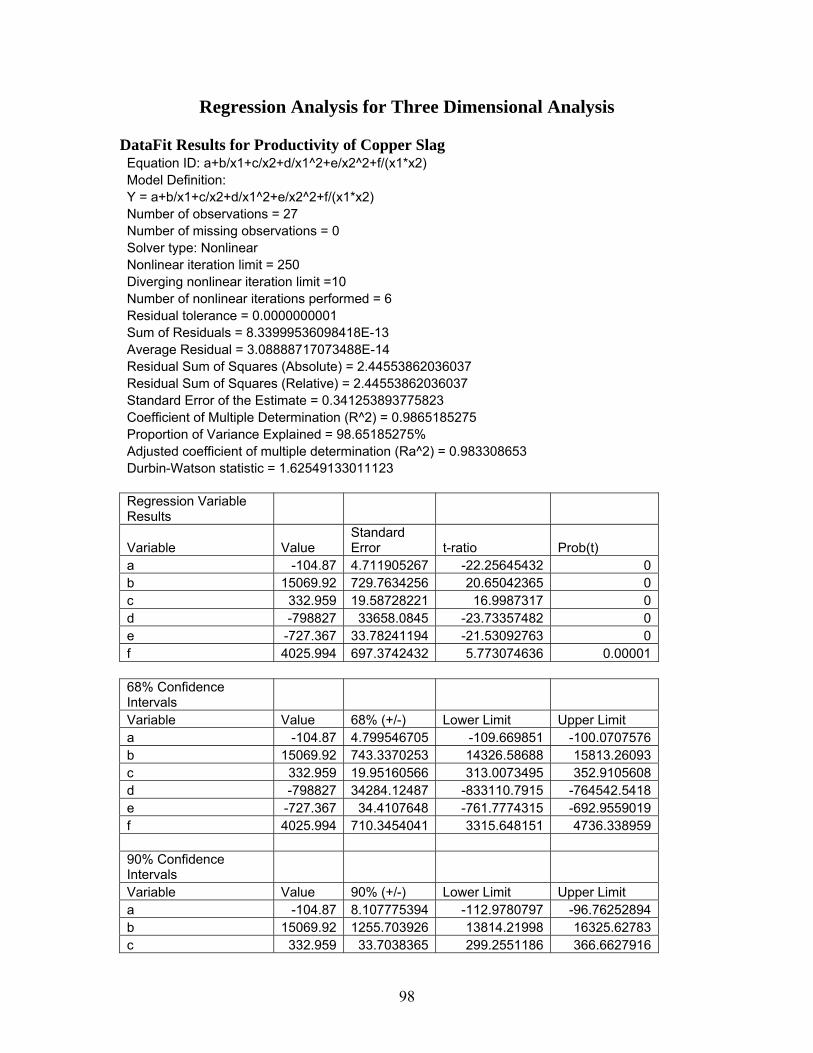
98
Regression Analysis for Three Dimensional Analysis
DataFit Results for Productivity of Copper Slag Equation ID: a+b/x1+c/x2+d/x1^2+e/x2^2+f/(x1*x2) Model Definition: Y = a+b/x1+c/x2+d/x1^2+e/x2^2+f/(x1*x2) Number of observations = 27 Number of missing observations = 0 Solver type: Nonlinear Nonlinear iteration limit = 250 Diverging nonlinear iteration limit =10 Number of nonlinear iterations performed = 6 Residual tolerance = 0.0000000001 Sum of Residuals = 8.33999536098418E-13 Average Residual = 3.08888717073488E-14 Residual Sum of Squares (Absolute) = 2.44553862036037 Residual Sum of Squares (Relative) = 2.44553862036037 Standard Error of the Estimate = 0.341253893775823 Coefficient of Multiple Determination (R^2) = 0.9865185275 Proportion of Variance Explained = 98.65185275% Adjusted coefficient of multiple determination (Ra^2) = 0.983308653 Durbin-Watson statistic = 1.62549133011123 Regression Variable Results
Variable Value Standard Error t-ratio Prob(t)
a -104.87 4.711905267 -22.25645432 0 b 15069.92 729.7634256 20.65042365 0 c 332.959 19.58728221 16.9987317 0 d -798827 33658.0845 -23.73357482 0 e -727.367 33.78241194 -21.53092763 0 f 4025.994 697.3742432 5.773074636 0.00001 68% Confidence Intervals Variable Value 68% (+/-) Lower Limit Upper Limit a -104.87 4.799546705 -109.669851 -100.0707576 b 15069.92 743.3370253 14326.58688 15813.26093 c 332.959 19.95160566 313.0073495 352.9105608 d -798827 34284.12487 -833110.7915 -764542.5418 e -727.367 34.4107648 -761.7774315 -692.9559019 f 4025.994 710.3454041 3315.648151 4736.338959 90% Confidence Intervals Variable Value 90% (+/-) Lower Limit Upper Limit a -104.87 8.107775394 -112.9780797 -96.76252894 b 15069.92 1255.703926 13814.21998 16325.62783 c 332.959 33.7038365 299.2551186 366.6627916

99
d -798827 57915.466 -856742.1327 -740911.2007 e -727.367 58.12939622 -785.4960629 -669.2372705 f 4025.994 1199.97186 2826.021695 5225.965415 95% Confidence Intervals Variable Value 95% (+/-) Lower Limit Upper Limit a -104.87 9.798878194 -114.6691825 -95.07142614 b 15069.92 1517.61602 13552.30789 16587.53992 c 332.959 40.73371209 292.225243 373.6926672 d -798827 69995.35253 -868822.0192 -728831.3141 e -727.367 70.25390386 -797.6205705 -657.1127628 f 4025.994 1450.259476 2575.734079 5476.253031 99% Confidence Intervals Variable Value 99% (+/-) Lower Limit Upper Limit a -104.87 13.34128857 -118.2115929 -91.52901576 b 15069.92 2066.252163 13003.67174 17136.17607 c 332.959 55.45943086 277.4995243 388.418386 d -798827 95299.50046 -894126.1671 -703527.1662 e -727.367 95.65152115 -823.0181878 -631.7151455 f 4025.994 1974.545432 2051.448123 6000.538987 Variance Analysis
Source DF Sum of Squares Mean Square F Ratio Prob(F)
Regression 5 178.9544243 35.79088487 307.338668 0 Error 21 2.44553862 0.11645422 Total 26 181.399963
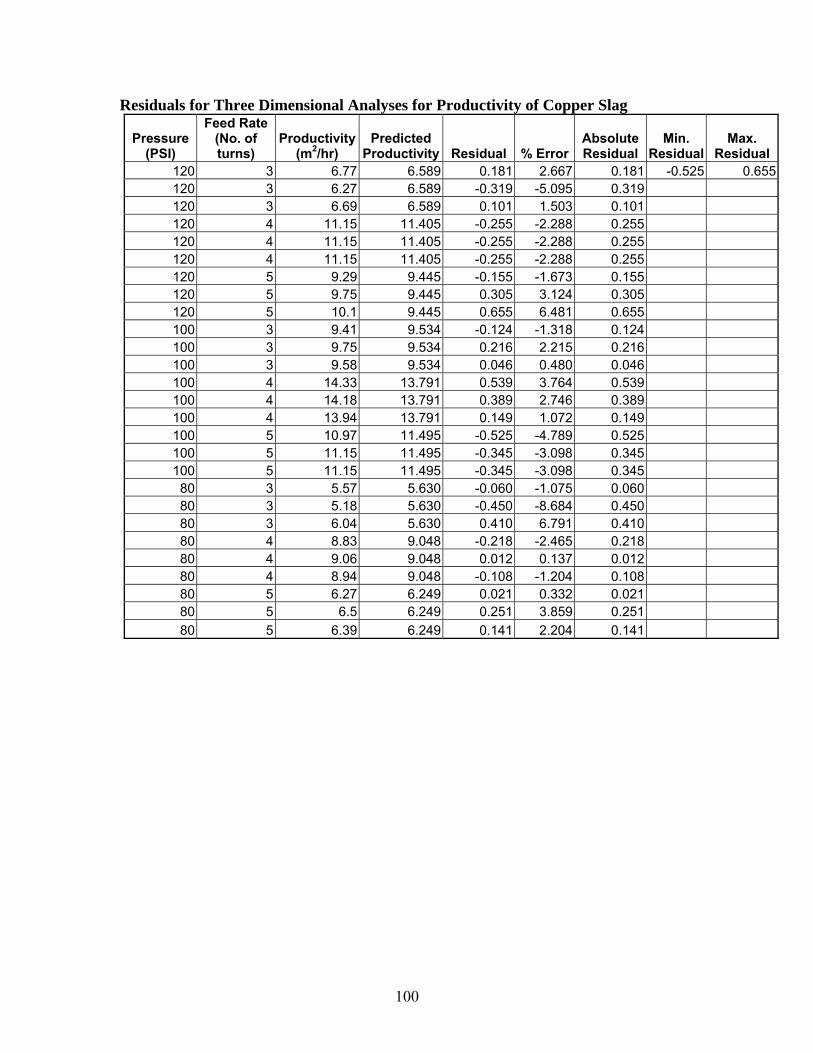
100
Residuals for Three Dimensional Analyses for Productivity of Copper Slag
Pressure (PSI)
Feed Rate (No. of turns)
Productivity (m2/hr)
Predicted Productivity Residual % Error
Absolute Residual
Min. Residual
Max. Residual
120 3 6.77 6.589 0.181 2.667 0.181 -0.525 0.655120 3 6.27 6.589 -0.319 -5.095 0.319 120 3 6.69 6.589 0.101 1.503 0.101 120 4 11.15 11.405 -0.255 -2.288 0.255 120 4 11.15 11.405 -0.255 -2.288 0.255 120 4 11.15 11.405 -0.255 -2.288 0.255 120 5 9.29 9.445 -0.155 -1.673 0.155 120 5 9.75 9.445 0.305 3.124 0.305 120 5 10.1 9.445 0.655 6.481 0.655 100 3 9.41 9.534 -0.124 -1.318 0.124 100 3 9.75 9.534 0.216 2.215 0.216 100 3 9.58 9.534 0.046 0.480 0.046 100 4 14.33 13.791 0.539 3.764 0.539 100 4 14.18 13.791 0.389 2.746 0.389 100 4 13.94 13.791 0.149 1.072 0.149 100 5 10.97 11.495 -0.525 -4.789 0.525 100 5 11.15 11.495 -0.345 -3.098 0.345 100 5 11.15 11.495 -0.345 -3.098 0.345
80 3 5.57 5.630 -0.060 -1.075 0.060 80 3 5.18 5.630 -0.450 -8.684 0.450 80 3 6.04 5.630 0.410 6.791 0.410 80 4 8.83 9.048 -0.218 -2.465 0.218 80 4 9.06 9.048 0.012 0.137 0.012 80 4 8.94 9.048 -0.108 -1.204 0.108 80 5 6.27 6.249 0.021 0.332 0.021 80 5 6.5 6.249 0.251 3.859 0.251 80 5 6.39 6.249 0.141 2.204 0.141

101
Residual Scatter Diagram for Productivity of Copper Slag Residual Scatter Diagram
-0.600
-0.400
-0.200
0.000
0.200
0.400
0.600
0.800
4.000 6.000 8.000 10.000 12.000 14.000 16.000
Predicted Productivity
Res
idua
l
Residual
Residual Normality Probability Plot for Productivity of Copper Slag

102
Observed vs. Predicted values of Productivity for Copper Slag at 120 PSI
Observed Vs Predicted Productivity for Copper Slag at 120 PSI
6
7
8
9
10
11
12
2 3 4 5 6
Feed Rate (Number of Turns)
Prod
uctiv
ity (m
2 /hr)
ObservedProductivity
PredictedProductivity
103
APPENDIX C: Material Data Safety Sheets

104
MSDS for Coal Slag
MATERIAL SAFETY DATA SHEET
SECTION I – GENERAL Reed Minerals, Harsco Corporation Product Name: Black Beauty Abrasives and Reed Minerals Roofing P.O. Box 0515 Products Camp Hill, PA 17001-0515 CAS Number: 68476-96-0 Emergency Telephone Number Common Name: Slag, Coal (717) 763-4200 Date: August 05, 2005 SECTION II – PRODUCT COMPOSITION Component Normal Composition (WT %) Range CAS Number OSHA PEL (mg/m3) Silicon Dioxide [SiO2] 41-53% 7631-86-9 80 mg/m3
%SiO2 Quartz <0.1% 14808-60-7 10 mg/m3
[Respirable Dust] %SiO2+2 Cristobalite ND 14464-46-1 30 mg/m3 [Quartz
Total Dust] %SiO2+2 Tridymite ND 15468-32-3 80 mg/m3
[Respirable Dust] %SiO2 Aluminum Oxide [Al2O3] 17-25% 1344-28-1 15 mg/m3 Calcium Oxide [CaO] 3-15% 1305-78-8 5 mg/m3 Magnesium Oxide [MgO] 0-4% 1309-48-4 15 mg/m3 (Fume) Iron Oxide [FeO] 7-31% 1309-37-1 10 mg/m3 Potassium Oxide [K2O] 0-3% 12136-45-7 NE Titanium Dioxide [TiO2] 0-2% 13463-67-7 15 mg/m3 ND - Not Detectable NE - Not Established SECTION III – PHYSICAL DATA Physical Form: Solid (Angular Granules) Boiling Temperature: N/A Melting Temperature: > 2500° F Vapor Pressure/Density: N/A Evaporation Rate: N/A Specific Gravity: 2.7 g/cc Typical Water Solubility: Negligible Color: Black Coarse Solid Odor: None
105
SECTION IV – FIRE/EXPLOSION/ REACTIVITY DATA Product is nonflammable, non-explosive and stable under normal conditions of use, storage and transportation. SECTION V – HEALTH HAZARD DATA EXPOSURE LIMITS: Refer to Section II which highlights the Permissible Exposure Limit (PEL). This limit is published and enforced by OSHA as a legal standard. Most PELs are expressed as eight hour average airborne concentrations. The nuisance dust exposure standard should be followed if exceeded than the appropriate respiratory protection equipment should be worn. ACUTE and CHRONIC TOXICITY: Exposure to and contact from dust may irritate the respiratory system, eyes, or skin. Coal slag is not listed on the NTP, IARC, or OSHA list of carcinogens. If ingested it may cause nausea and vomiting. FIRST AID: 1. Eye Contact – Immediately flush eyes thoroughly with water or an ophthalmic saline solution.* 2. Skin Contact – Wash skin with soap and water if irritation occurs.* 3. Inhalation – Remove affected person(s) to fresh air source.* 4. Oral intake – Rinse mouth out with water.* *Note: if symptoms persist, contact a physician or other medical personnel. SECTION VI – CONTROL MEASURES RESPIRATOR PROTECTION: If airborne concentrations exceed recommended exposure limits, a suitable NIOSH/MSHA approved filter respirator should be worn. General ventilation or local exhaust is normally adequate to control dust emissions, if not engineering controls should be utilized. EYE: Safety glasses with side shields should be worn as minimum protection from impact. Dust goggles should be worn when excessively dusty conditions are present or anticipated. GENERAL: The use of hard hats and hard toe shoes is recommended. Gloves may be worn to protect from abrasion as well as long sleeve shirts to minimize dermal exposure and potential skin irritation. SECTION VII – SPILL, LEAK, AND DISPOSAL PROCEDURES No special procedures required for clean-up, but it is recommended that this is done mechanically or through the use of hand tools. Wetting with water will reduce any airborne dust. Uncontaminated product does not exceed Toxicity Characteristic Leaching Procedure (TCLP) limits and may be disposed of as an inert material in an appropriate solid waste landfill according to applicable Federal, State and Local regulations.
Disclaimer
The opinions expressed herein are those of competent personnel within Harsco Corporation. Harsco believes that the information contained herein is current and accurate for the normal and intended use of this product as of the date of this Material Safety Data Sheet. Since the use of this information and of those opinions or the conditions of use of the product are not within the control of Harsco Corporation, it is the user's obligation to determine and observe the conditions of safe use and disposal of the product by their operations. Harsco Corporation will not be liable for any loss, damage or injury arising out of the use thereof.

106
MSDS for Copper Slag

107

108
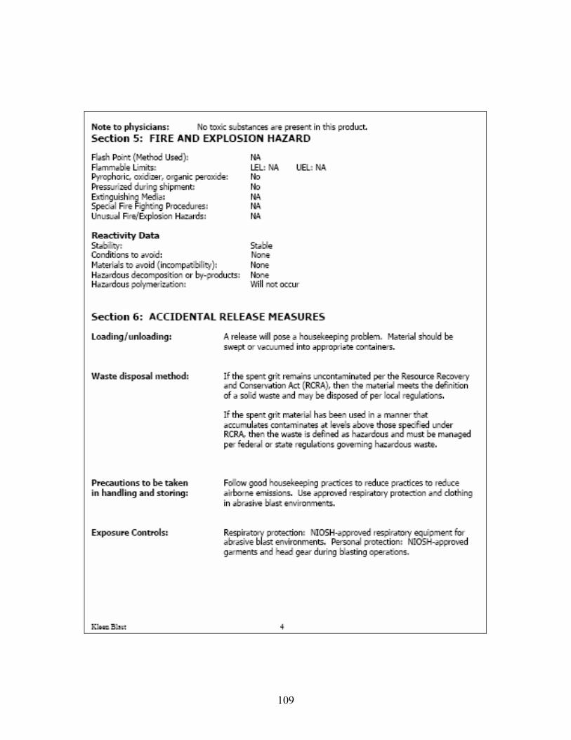
109

110

111
MSDS for Specialty Sand 1. PRODUCT/COMPANY IDENTIFICATION
Manufacturer’s Name & Address:
Titan America LLC
1151 Azalea Garden Rd.
Norfolk, VA 23502
Telephone Number for Information:
1.800.468.7622
Emergency Telephone:
1.757.858.6500
2. COMPOSTION INFORMATION
Chemical Name CAS Registry Number % (approx.)
Natural Sand* NA 100
*May contain crystallline silica 14808-60-7 >1
3. PHYSICAL/CHEMICAL CHARACTERISTICS
Boiling Point N/A
Specific Gravity (H2O = 1) 2.55-2.80
Vapor Pressure (mm Hg) N/A
Melting Point N/A
Vapor Density (AIR-1) N/A
Evaporation Rate N/A
Solubility in Water Not soluble
Appearance & Odor Fine grains, yellow to white in color; no odor.

112
4. FIRE AND EXPLOSION HAZARD DATA
Flash Point N/A
Extinguishing Media N/A
Special Fire Fighting Procedures None
Unusual Fire & Explosion Hazards None
Flammable Limits N/A
LEL N/A
UEL N/A
Trade Name:
Sand
Chemical Name and Synonyms
Natural Sand*, Construction Aggregate
Department of Transportation Identification No.:
None
*Composition varies naturally, typically contains crystalline silica
5. REACTIVITY DATA
Stability: Stable. Avoid contact with incompatible materials.
Incompatibility: Contact with powerful oxidizing agents such as fluorine, boron
trifluoride, chlorine trifluoride,
manganese trifluoride, and oxygen difluoride may cause fire and/or explosions. Silica
dissolves in hydrofluoric acid producing a corrosive gas-silicon tetrafluoride.
Hazardous Decomposition or Byproducts: Respirable dust particles may be generated
when sand is moved or ground.

113
Hazardous Polymerization: Will not occur. No conditions to avoid.
6. HEALTH HAZARD DATA AND FIRST AID
EXPOSURE LIMITS:
Unless specified otherwise, limits are expressed as a time-weighted average (TWA)
concentration for an 8-hour work shift of a 40-hour workweek. Limits for cristobalite and
tridymite (other forms of crystalline silica) are equal to one-half the limits for quartz.
ABBREVIATIONS:
ACGIH TLV: Threshold limit value of the American Conference of Governmental
Industrial Hygienists (ACGIH).
mg/m3: Milligrams of substance per cubic meter of air.
NIOSH REL: Recommended exposure limit of the National Institute for Occupational
Safety and Health (NIOSH), expressed as a TWA
concentration for up to a 10-hour work-day during a 40-hour workweek.
OSHA PEL: Permissible exposure limit of the federal Occupational Safety and Health
Administration (OSHA).
Crystalline Silica SiO2: OSHA PELs (respirable fraction) [10 mg/m3 ÷ (% SiO2+2)],
(total dust) [30 mg/m3 ÷ (% SiO2+2)]; ACGIH TLV (respirable
fraction) 0.05 mg/m3, NIOSH REL (respirable fraction) 0.05 mg/m3.
Other Particulates: OSHA PEL (total particulate, not otherwise regulated) 15 mg/m3,
(respirable particulate, not otherwise regulated) 5 mg/m3,
ACGIH TLV (nuisance particulates) 10 mg/m3 (inhalable), 5 mg/m3 (respirable).
HEALTH HAZARDS:
Primary Route(s) of Entry:
114
Inhalation: Yes
Skin: No
Ingestion: No
Acute:
Eye Contact: Minor irritation to the eyes or nose.
Inhalation: Dusts may irritate the nose, throat, and respiratory tract by mechanical
abrasion. Coughing, sneezing, and shortness of breath may occur following exposures in
excess of appropriate exposure limits.
Skin Contact: Direct contact may cause irritation by mechanical abrasion.
Ingestion: Expected to be practically non-toxic. Ingestion of large amounts may cause
gastrointestinal irritation and blockage.
Chronic:
Inhalation: Chronic exposure to respirable dust in excess of appropriate exposure limits
may cause lung disease. Silicosis may result from excessive exposure to respirable silica
dust for prolonged periods. Not all individuals with silicosis will exhibit symptoms.
Silicosis is progressive and symptoms can appear at any time, even after exposure has
ceased. Symptoms may include shortness of breath, coughing, or right heart enlargement
and/or failure. Persons with silicosis have an increased risk of pulmonary tuberculosis
infection. Tobacco smoking may increase the risk of developing lung disorders, including
emphysema and lung cancer.
Carcinogenicity: Crystalline silica is classified by the International Agency for Research
on Cancer (IARC) as a carcinogenic to humans (Group 1). The National Toxicology

115
Program (NTP) has characterized respirable silica as “known to be a human carcinogen”.
Prolonged and repeated breathing of silica may cause lung cancer.
Signs & Symptoms of Exposure: Dust irritation of eyes and/or respiratory system.
Medical Conditions Generally Aggravated by Exposure: Inhaling respirable dust may
aggravate existing respiratory system disease(s) and/or dysfunctions such as emphysema
or asthma. Exposure may aggravate existing eye conditions.
EMERGENCY & FIRST AID PROCEDURES:
Eyes: Immediately flush eye(s) with plenty of clean water for at least 15 minutes, while
holding the eyelid(s) open. Beyond flushing, do not attempt to remove material from the
eye(s). Contact a physician if irritation persists or later develops.
Inhalation: Remove to fresh air. Dust in throat and nasal passages should clear
spontaneously. Contact a physician if irritation persists or later develops.
Skin: Wash with soap and water. Contact a physician if irritation persists or later
develops.
Ingestion: If person is conscious, give large quantity of water and induce vomiting;
however, never attempt to make an unconscious person drink or vomit. Get immediate
medical attention.
7. PERSONAL PROTECTION AND CONTROL MEASURES
Ventilation: Local exhaust or general ventilation adequate to maintain exposures below
appropriate exposure limits.
Other: Respirable dust and silica levels should be monitored regularly. Dust and silica
levels in excess of appropriate exposure limits should be reduced by all feasible

116
engineering controls, including (but not limited to) wet suppression, ventilation, process
enclosure, and enclosed employee work stations.
Respiratory Protection: When dust or silica levels exceed or are likely to exceed
appropriate exposure limits, follow MSHA or OSHA regulations, as appropriate, for use
of NIOSH-approved respiratory protection equipment.
Skin Protection: Protective gloves should be worn to prevent mechanical injury.
Eye Protection: Safety glasses with side shields should be worn as minimum protection.
Dust goggles should be worn when excessive (visible) dust conditions are present or
anticipated. Contact lenses should not be worn when working with this product.
Hygiene: Ordinary personal hygiene.
8. STORAGE AND HANDLING PRECAUTIONS
Respirable silica and dust may be generated during processing, handling, and storage.
The personal protection and controls identified in Section VII of the MSDS should be
applied as appropriate.
9. SPILL, LEAK AND DISPOSAL PRACTICES
The personal protection and controls identified in Section VII of the MSDS should be
applied as appropriate.
Steps to Be Taken if Material Is Released or Spilled: Spilled materials, where dust can be
generated, may overexpose cleanup personnel to respirable silica and dust. Wetting of
spilled material and/or use of respiratory protective equipment may be necessary. Do not
dry sweep spilled material.
Waste Disposal Method: Dispose of waste materials only in accordance with applicable
federal, state, and local laws and regulations.

117
NOTICE: Based on research of available data, Titan America LLC believes that the
information contained in this Material Safety Data Sheet is accurate. The suggested
procedures are based on data and experience as of the date of preparation of the MSDS.
The suggestions should not be confused with nor followed in violation of applicable laws,
regulations, rules or insurance requirements. Titan America LLC’s voluntary preparation
of this MSDS should not be construed, in any way, as an agreement to be subject to
OSHA jurisdiction.

118
APPENDIX D: Example for Calculation of Blasting Costs
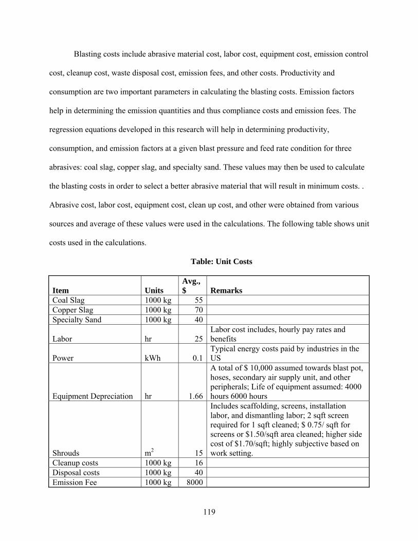
119
Blasting costs include abrasive material cost, labor cost, equipment cost, emission control
cost, cleanup cost, waste disposal cost, emission fees, and other costs. Productivity and
consumption are two important parameters in calculating the blasting costs. Emission factors
help in determining the emission quantities and thus compliance costs and emission fees. The
regression equations developed in this research will help in determining productivity,
consumption, and emission factors at a given blast pressure and feed rate condition for three
abrasives: coal slag, copper slag, and specialty sand. These values may then be used to calculate
the blasting costs in order to select a better abrasive material that will result in minimum costs. .
Abrasive cost, labor cost, equipment cost, clean up cost, and other were obtained from various
sources and average of these values were used in the calculations. The following table shows unit
costs used in the calculations.
Table: Unit Costs
Item Units Avg., $ Remarks
Coal Slag 1000 kg 55 Copper Slag 1000 kg 70 Specialty Sand 1000 kg 40
Labor hr 25Labor cost includes, hourly pay rates and benefits
Power kWh 0.1Typical energy costs paid by industries in the US
Equipment Depreciation hr 1.66
A total of $ 10,000 assumed towards blast pot, hoses, secondary air supply unit, and other peripherals; Life of equipment assumed: 4000 hours 6000 hours
Shrouds m2 15
Includes scaffolding, screens, installation labor, and dismantling labor; 2 sqft screen required for 1 sqft cleaned; $ 0.75/ sqft for screens or $1.50/sqft area cleaned; higher side cost of $1.70/sqft; highly subjective based on work setting.
Cleanup costs 1000 kg 16 Disposal costs 1000 kg 40 Emission Fee 1000 kg 8000

120
First, emission factors, productivity, and consumption are calculated for the three
materials using equations 2, 4, and 5 and their coefficients respectively. These values and unit
costs were then used to determine blasting costs per 1000 m2 area cleaned. The following table
shows the calculation methods and blasting costs. From this example, it evident that copper slag
results in minimum costs. Material cost, labor cost, emission costs etc. vary from one supplier to
another and one state to another. Using the actual costs and including addition costs incurred by
the industries, more accurate costs can be estimated. This will greatly help industries in material
selection and process optimization.
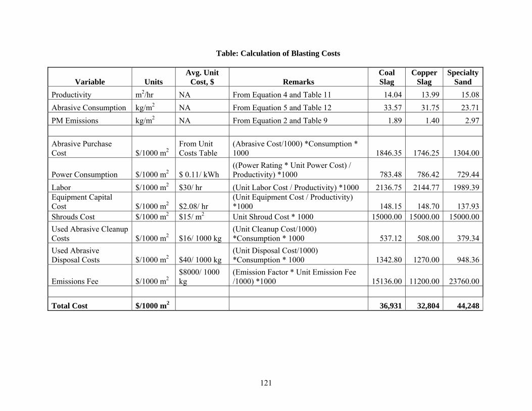
121
Table: Calculation of Blasting Costs
Variable Units Avg. Unit
Cost, $ Remarks Coal Slag
Copper Slag
Specialty Sand
Productivity m2/hr NA From Equation 4 and Table 11 14.04 13.99 15.08Abrasive Consumption kg/m2 NA From Equation 5 and Table 12 33.57 31.75 23.71PM Emissions kg/m2 NA From Equation 2 and Table 9 1.89 1.40 2.97 Abrasive Purchase Cost $/1000 m2
From Unit Costs Table
(Abrasive Cost/1000) *Consumption * 1000 1846.35 1746.25 1304.00
Power Consumption $/1000 m2 $ 0.11/ kWh ((Power Rating * Unit Power Cost) / Productivity) *1000 783.48 786.42 729.44
Labor $/1000 m2 $30/ hr (Unit Labor Cost / Productivity) *1000 2136.75 2144.77 1989.39Equipment Capital Cost $/1000 m2 $2.08/ hr
(Unit Equipment Cost / Productivity) *1000 148.15 148.70 137.93
Shrouds Cost $/1000 m2 $15/ m2 Unit Shroud Cost * 1000 15000.00 15000.00 15000.00Used Abrasive Cleanup Costs $/1000 m2 $16/ 1000 kg
(Unit Cleanup Cost/1000) *Consumption * 1000 537.12 508.00 379.34
Used Abrasive Disposal Costs $/1000 m2 $40/ 1000 kg
(Unit Disposal Cost/1000) *Consumption * 1000 1342.80 1270.00 948.36
Emissions Fee $/1000 m2 $8000/ 1000 kg
(Emission Factor * Unit Emission Fee /1000) *1000 15136.00 11200.00 23760.00
Total Cost $/1000 m2 36,931 32,804 44,248

122
VITA Kalpalatha Kambham was born in Piler, India in 1978. She graduated with a Bachelor of
Engineering in Civil Engineering from Sri Venkateswara University College of Engineering,
India in 1999 and a Master of Science in Civil Engineering from University of New Orleans in
2002. Her areas of interest are air pollution control, air quality modeling, waste management,
industrial hygiene, risk assessment, and development of Expert Management Systems.