performance evaluation of the ordinary least square (ols

South African Journal of Geomatics, Vol. 6. No. 1, April 2017

73

Performance Evaluation of the Ordinary Least Square (OLS) and Total

Least Square (TLS) in Adjusting Field Data: An Empirical Study on a

DGPS Data

M. S. Peprah1, I. O. Mensah1*

1Deparment of Geomatic Engineering, University of Mines and Technology, Tarkwa, Ghana.

*Corresponding authors email: [email protected]; [email protected]

DOI: http://dx.doi.org/10.4314/sajg.v6i1.5

Abstract

Survey measurements have become the traditional means of obtaining point positions by

most surveyors over the centuries. The assertion that a post processed DGPS field data is

precise, accurate and can be used to execute any engineering works due to its minimum

human errors need to be reviewed; this is because the post processed field data still contains

errors and needs to be adjust. Adjustments and computations is one of the main research

field in mathematical and satellite geodesy to assess the magnitude of errors and to study

their distributions whether they are within or not within the acceptable tolerance. In order

to achieve the objective of this study, a DGPS field data was adjusted using the Ordinary

Least Square (OLS) and Total Least Square (TLS) techniques. The OLS considers errors

only in the observation matrix, and adjusts observations in order to make the sum of its

residuals minimum. The TLS considers errors in both the observation matrix and the data

matrix, thereby minimizing the errors in both matrices. The limited availability of

information on OLS and TLS in adjusting DGPS field data and the uncertainty of which

method is optimal, whether the OLS and TLS is the most appropriate technique has called

for the need to undertake this study. This study aimed at comparing the working efficiency

of the OLS and TLS, assessing their individual accuracy and selecting the most effective

method in adjusting DGPS field data. Each model was assessed based on statistical

indicators of mean horizontal error (MHE), mean bias error (MBE), mean absolute error

(MAE), root mean square error (RMSE), and standard deviation (SD). After applying the

OLS and TLS methods independently for the same datasets, it was ascertained that, the OLS

method was better in adjusting DGPS field data than the TLS with a MHE and SD of

+1.203079 m and +1.663134 m as compared to TLS with MHE and SD of +7.0985507 m

mailto:[email protected]

http://dx.doi.org/10.4314/sajg.v6i1.5


74

and +2.594045 m respectively. This study will therefore create opportunity for geospatial

professionals to know the efficiency of OLS and TLS in solving some of the problems in

mathematical and satellite geodesy.

Keywords: Differential Global Positioning, System, Total Least Square, Ordinary Least

Square, Survey Adjustments, Horizontal Position Displacement.

1. Introduction

Survey measurements over the centuries have been the traditional means of

measuring and portraying the earth’s surface (Ghilani and Wolf, 2012). The measurement

can be either direct or indirect (Ghilani, 2010). Survey measurements are one of the core

mandate in all areas of geoscientific applications. The fundamental measured quantities in

every survey measurements are distances, angles, and elevations. These forms the basis for

coordinates determination of positions concerning a specific datum either horizontal or

vertical (Annan et al., 2016a). From these coordinates positions, other distances and angles

that were not obtained directly during field measurements may be computed indirectly. The

errors that were present in the original direct observations may propagate by the

computational process into the indirect values (Ghilani, 2010). Thus, the indirect

measurements contain errors that are functions of the original errors (Ghilani, 2010). In

adjusting the field data values, the traditional techniques that are normally used is the

classical least squares techniques.

Classical least square techniques are the most widely used methods for adjusting

field data of ground points. In the classical least square techniques, adjustment of the

observation equations where only the observations are considered as stochastic (Acar et al.,

2006). In some instances, the design matrix elements contain errors which are usually

ignored in the classical least techniques and this ignorance remains as an uncertainty in the

solution results (Acar et al., 2006).

Differential Global Positioning System (DGPS) is of a higher accuracy than the

absolute observation due to the use of reference station where coordinates are known to

ascertain accuracy. The techniques used in DGPS observations are static, fast static, stop

and go, and real time kinematics. Among DGPS survey techniques, the static method is of


75

a higher accuracy due to some techniques used in the data collection process. Data collected

after field survey needs to be processed to obtain a desired result. DGPS data after post

processing still contain errors (Ansah, 2016; Okwuashi, 2014). The errors remain in the data

could be adjusted. Several adjustment methods exist such as ordinary least squares (Annan

et al., 2016a; Okwuashi and Eyoh, 2012a), Total least squares (Acar et al., 2006; Annan et

al., 2016b; Okwuashi and Eyoh, 2012b), robust estimation (Wieser and Brunner, 2001),

least square collocation (LSC) (Moritz, 1972). Conversely, there is a common belief that

data obtain from the GPS instrument are very precise and accurate due to less interference

of humans in the collection process and can be used to execute any given task without further

adjustments.

The measured field data like any other survey measurement contains errors and need

to be adjusted. Usually, adjustment is done using classical approach such as ordinary least

approach (Annan et al., 2016a; Okwuashi & Eyoh, 2012b), but the ordinary least square

which is based on regression analysis considers only the observations to be stochastic (Acar

et al., 2006) and thus account for errors only in the observation vector. Conversely, there

exist errors in both the design and observation matrices which ought to be modelled out

(Annan et al., 2016a). OLS is the most commonly widely used adjustment method in

geodesy. It has been used in many geodetic areas in the recent decades. Notable among them

are approximation of the surfaces in engineering structures (Lenda, 2008), finding the

relationship between global and Cartesian coordinates (Ziggah, 2012), predictions of local

coordinates (Odutola et al., 2013), converting GPS data from global coordinate system to

the National coordinate system (Dawod et al., 2011).

Another numerical method applicable for adjusting field data is the TLS. It is worth

mentioning that several studies have been carried out by researchers with the TLS

techniques. Notable among them are 3D datum transformation including the weighted

scenarios (Amiri-Simkooei and Jazaeri, 2012), measuring data perturbation size (Markovsk

et al., 2009), localization of robots (Yang, 1997), calibration of robots (Nievergelt, 1994).

It was emphasized that OLS which was mostly used in early times gave less accuracies

because it assumes errors only in the output variable, y-value, whereas TLS assumes errors

in both the input and output variables (Effah, 2015). The total least squares (TLS) was

invented to resolve the working efficiency of the OLS (Annan et al., 2016a). The TLS have

the ability to adjust the errors in both the observation matrix and design matrix (Acar et al.,

2006) in order to yield a better estimate. The limited availability of technical papers in


76

geodesy on TLS have called for the need to undergone this study. Also, the optimal model

in adjusting surveying networks whether the OLS and TLS is good enough is the objective

of this present study. Researchers such as (Acar et al., 2006; Annan et al., 2016a, 2016b;

Okwuashi and Eyoh, 2012; OKwuashi, 2014) have applied TLS to solve many scientific

problems and they concluded the TLS working efficiency is encouraging. This present study

adopted the OLS and TLS in adjusting DGPS network and to propose the models which is

optimal for adjusting DGPS network.

Although extensive applications of OLS and TLS have been carried out, limited

literature is available in geodesy technical papers on the applications of OLS and TLS, for

adjusting DGPS field data especially in developing countries like Ghana where geodesy has

not yet reached the advanced stage. In addition, there have been arguments on which

method, whether the OLS or TLS model is the most effective based on their various

ideologies. Thus, the TLS technique takes into account observational errors on both

dependent and independent variables while OLS considers only the independent variable.

Therefore, this present study aims at making a comparative study of both methods and

selecting the most effective technique. The authors were motivated to embark this study

because it is yet to be evaluated in Ghana. This study will also create the opportunity for

geospatial professionals to arrive a conclusion on which technique is optimal in adjusting

DGPS field after post processing.

2. Study Area and Data Source

The study area (Figure 1) is situated in the mining town of Tarkwa which is the

administrative capital of the Tarkwa Nsuaem Municipal Assembly in the Western Region

of Ghana. It is found in the Southwest of Ghana with geographical coordinates between

longitudes 1ᵒ 59′ 00″ W and latitude 5ᵒ 18′ 00″ N and is 78 m above mean sea level. It is

about 85 km from Takoradi, which is the regional capital, 233 km from Kumasi and about

317 km from Accra (Ziggah, 2012). The topography is generally described as remarkable

series of ridges and valleys. The ridges are formed by the Banket and Tarkwa Phyllites

whereas upper quartzite and Huni Sandstone are present in the valleys. Surface gradients of

the ridges are generally very close to the Banket and Tarkwa Phyllites. Its environs generally

lie within the mountain ranges covered by thick forest interjected by undulating terrain with

few scarps. The study area has a South-western Equatorial climate with seasons influenced


77

by the moist South-West Monsoon winds from the Atlantic Ocean and the North-East Trade

Winds. The mean rainfall is approximately 1500 mm with peaks of more than 1700 mm in

June and October. Between November and February, the rainfall pattern decreases to

between 20 mm to 90 mm (Forson, 2006). The mean annual temperature is approximately

25 ᵒC with small daily temperature variations. Relative humidity varies from 61 % in January

to a maximum of 80 % in August and September (Ziggah, 2012; Seidu, 2004).

Figure 1. Study Area

In this study, a total of 12 DGPS data collected by field measurements in UMaT,

Tarkwa, Ghana, situated in West Africa, were used in the OLS and TLS model formulation.

It is well acknowledged that, one of the contributing factors affecting the estimation

accuracy of models is related to the quality of datasets used in model-building (Dreiseitl and


78

Ohno-Machado, 2002; Ismail et al., 2012). Therefore, to ensure that the obtained field data

from the GPS receivers are reliable and accurate, several factors such as checking of

overhead obstruction, obstruction, observation period, observation principles and

techniques as suggested by many researchers (Yakubu and Kumi-Boateng, 2011; Ziggah et

al., 2016) were performed on the field. In addition, all potential issues relating to GPS

survey work were also considered.

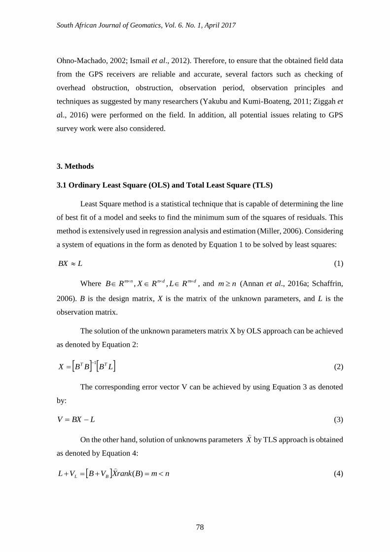
3. Methods

3.1 Ordinary Least Square (OLS) and Total Least Square (TLS)

Least Square method is a statistical technique that is capable of determining the line

of best fit of a model and seeks to find the minimum sum of the squares of residuals. This

method is extensively used in regression analysis and estimation (Miller, 2006). Considering

a system of equations in the form as denoted by Equation 1 to be solved by least squares:

LBX (1)

Where dmdnnm RLRXRB ,, , and nm (Annan et al., 2016a; Schaffrin,

2006). B is the design matrix, X is the matrix of the unknown parameters, and L is the

observation matrix.

The solution of the unknown parameters matrix X by OLS approach can be achieved

as denoted by Equation 2:

LBBBX TT 1 (2)

The corresponding error vector V can be achieved by using Equation 3 as denoted

by:

LBXV (3)

On the other hand, solution of unknowns parameters X

by TLS approach is obtained

as denoted by Equation 4:

nmBrankXVBVL BL )(

(4)


79

Where VL is the error vector of observations and VB is the error matrix of the data

matrix, the assumption that both have independently and identically distributed rows with

zero mean and equal variance (Akyilmaz, 2007).

Golub and Van Loan, (1980), invented TLS to rectify the inefficiency

associated with the OLS. Thus, accounting for perturbations in data matrix and observation

matrix (Annan et al., 2016b). TLS is a mathematical algorithm that yields a unique solution

in analytical form in terms of the Singular Value Decomposition (SVD) of the data matrix

(Markovsky and Van Huffel, 2007). According to Golub and Van Loan, (1980) and

Okwuashi and Eyoh, (2012a), the TLS algorithm is an iterative process which looks to

minimize the errors in Equation 5 as denoted by:

)1(ˆ,ˆ,ˆ,ˆ,min mn

FRLBLBLB (5)

The optimization process goes on until a minimizing LB ˆ,ˆ is obtained, any X

that

satisfies LXB ˆˆˆ is the TLS solution (Annan et al., 2016a). In order to obtain the solution

of LXB ˆ , we write the functional relation as denoted by Equation 6:

01,, TTXLB (6)

The TLS problem can be solved using the Singular Value Decomposition (SVD)

(Markovsky and Van Huffel, 2007; Ge and Wu, 2012). The SVD of the augmented matrix

LB, is required to determine whether or not it is rank deficient. Matrix LB, can be

represented by SVD as denoted by Equation 7 as:

TUSVLB , (7)

Where U = real valued m x n orthonormal matrix, UUT = Im, V = real value n x n

orthonormal matrix, VVT = In, S = m x n matrix with diagonals being singular values, off-

diagonals are zeros. The rank of matrix LB, is m + 1, and must be reduced to m using the

Eckart-Young Mirsky theorem (Annan et al., 2016a). The TLS solution after the rank

reduction is given by Equation 8 denoted as:

1

1,1

11,ˆ

m

mm

T VV

X (8)


80

If 01,1 mmV , then Tmmmmm VVBVLBX 1,1,11,1 ,,)./(1 belongs to the column space

of B̂ , hence X solves the basic TLS problem (Okwuashi and Eyoh, 2012a). The

corresponding TLS correction is achieved by using Equation 9 as denoted by:

LBLBLB ˆˆ,ˆ,ˆ (9)

3.2 Models Performance Evaluation

In order to determine the accuracies of the models used, the various statistical

indicators were employed to determine the working efficiency of the models. Hence, to

make an unprejudiced valuation of the models, statistical indicators such as Root Mean

Square (RMSE), Mean Biased Error (MBE), and Mean Absolute Error (MAE), Horizontal

Position error (HE), and Standard Deviation were used. Their individual mathematical

languages are given by Equation 10 to Equation 14 respectively denoted by:

n

ERMSE

2

(10)

where n is the number of observation points and E2 is the square of the error. The MBE was

calculated using the formula below:

N

EMBE (11)

where E is the error and n is the number of observation points. The MAE was calculated

using the formula:

N

EMAE (12)

where |𝐸| is the absolute error and n is the number of observation points.

2

12

2

12 )()( YYXXHE 13

Where X2 and Y2 are the existing coordinates, and X1 and Y1 are the observed coordinates.

1

)( 2

n

xxSD 14


81

The Standard Deviation (SD) measures how closely the data are clustered around the mean.

n-1 is the degree of freedom.

4. Results and Discussions

Table 1 shows the existing coordinates and the observed DGPS data. From Table 1,

it was observed that, there is a difference between the existing data and the measured data.

Table 2 and Table 3 shows the results obtained by the OLS and TLS models. The residual

graphs for the OLS and TLS models are represented by Figure 2 and Figure 3. Figure 4 is

the horizontal shift error graph obtained by the OLS and TLS models. From the graph, it

was observed that the performance of the OLS model was encouraging as compared to the

TLS.

Table 1. Existing Coordinates and DGPS field Data (Units in metres)

ACTUAL ACTUAL DGPS DGPS RESIDUALS

X Y X Y ΔX ΔY

163244.2300 69656.2000 163244.2300 69656.2000 0.0000 0.0000

163216.6680 69604.4470 163216.5376 69604.3286 0.1304 0.1184

163363.5750 69380.3820 163363.1177 69380.1969 0.4573 0.1851

163463.0150 69520.9960 163462.4604 69520.7708 0.5546 0.2252

163505.7080 69583.2260 163505.2266 69582.9690 0.4814 0.2570

163509.1960 69598.9950 163509.0747 69599.0941 0.1213 -0.0991

163517.3220 69634.4160 163515.8068 69635.0266 1.5152 -0.6106

163531.1310 69786.7810 163529.5562 69787.1048 1.5748 -0.3238

163497.2520 69817.9670 163494.9389 69818.4032 2.3131 -0.4362

163423.3670 69777.2060 163422.5800 69776.7900 0.7870 0.4160

163394.6160 69753.3440 163392.7060 69753.3482 1.9100 -0.0042

163359.0890 69687.6660 163351.3071 69688.4810 7.7819 -0.8150

Table 2. Results obtained by the OLS models (Units in metres)

ACTUAL ACTUAL ADJUSTED DGPS OLS RESIDUALS

X Y X Y ΔX ΔY

163244.2300 69656.2000 163245.8392 69656.6958 -1.6092 -0.4958

163216.6680 69604.4470 163217.9890 69604.9549 -1.3210 -0.5079

163363.5750 69380.3820 163363.7027 69380.4783 -0.1277 -0.0963

163463.0150 69520.9960 163463.4563 69520.6158 -0.4413 0.3802

163505.7080 69583.2260 163506.4051 69582.6250 -0.6971 0.6010

163509.1960 69598.9950 163510.3055 69598.7258 -1.1095 0.2692


82

163517.3220 69634.4160 163517.1555 69634.6104 0.1664 -0.1944

163531.1310 69786.7810 163531.4144 69786.5363 -0.2834 0.2447

163497.2520 69817.9670 163496.9279 69817.9311 0.3241 0.0359

163423.3670 69777.2060 163424.4771 69776.5937 -1.1101 0.6123

163394.6160 69753.3440 163394.5438 69753.2700 0.0722 0.0740

163359.0890 69687.6660 163352.9523 69688.5891 6.1367 -0.9231

Table 3. Results obtained by the TLS model (Units in metres)

ACTUAL ACTUAL ADJUSTED DGPS TLS RESIDUALS

X Y X Y ΔX ΔY

163244.2300 69656.2000 163247.7070 69664.4334 -3.4770 -8.2334

163216.6680 69604.4470 163217.7791 69614.4181 -1.1111 -9.9711

163363.5750 69380.3820 163352.0532 69385.4190 11.5218 -5.0370

163463.0150 69520.9960 163457.2129 69519.7871 5.8021 1.2089

163505.7080 69583.2260 163502.5647 69579.2970 3.1433 3.9290

163509.1960 69598.9950 163507.1551 69595.0755 2.0409 3.9195

163517.3220 69634.4160 163515.5595 69630.3250 1.7625 4.0910

163531.1310 69786.7810 163536.5335 69780.2261 -5.4025 6.5549

163497.2520 69817.9670 163503.7753 69812.8890 -6.5233 5.0780

163423.3670 69777.2060 163430.1214 69775.1919 -6.7544 2.0141

163394.6160 69753.3440 163399.4096 69753.4291 -4.7936 -0.0851

163359.0890 69687.6660 163355.2823 69691.2106 3.8067 -3.5446

Figure 2 Residuals plot in the Eastings

-10

-5

0

5

10

15

20

1 2 3 4 5 6 7 8 9 10 11 12

X R

ESID

UA

LS (

m)

POINT ID

TLS

OLS

Observed


83

Figure 2 show the variations of residuals in eastings when the adjusted coordinates

produced by the TLS and OLS methods respectively were subtracted from the actual

existing coordinates. It was observed that the OLS method gave better estimates of the

unknowns as compared to the TLS. This could possibly be that perturbation exists in the

design matrix and the observation matrix formed from the coordinates obtained from the

study area. Therefore, the OLS was preferred to that of the TLS for the study area.

Figure 3 Residuals plot in the Northings

Similarly, Figure 3 show the variations of residuals in northings when the adjusted

coordinates produced by the TLS and OLS methods respectively were subtracted from the

actual existing coordinates. It was observed that the OLS method gave better estimates of

the unknowns as compared to the TLS. This could possibly be that perturbation exists in the

design matrix and the observation matrix formed from the coordinates obtained from the

study area. Therefore, the OLS was preferred to that of the TLS for the study area.

The horizontal shifts of the positions for all the twelve points for both OLS and TLS

methods were computed and the results is shown in Table 4. Figure 4 show the plot of the

horizontal shift of the OLS and TLS models.

-12

-10

-8

-6

-4

-2

0

2

4

6

8

1 2 3 4 5 6 7 8 9 10 11 12

Y R

ESID

UA

LS (

m)

POINT ID

TLS

OLS

Observed


84

Table 4 Horizontal Displacement of Points (Units in metres)

POINT ID OBSERVED OLS TLS

1 0.000000 1.683847 8.937472

2 0.176133 1.415275 10.03282

3 0.493341 0.159941 12.57471

4 0.598578 0.582493 5.926703

5 0.545706 0.920407 5.031637

6 0.156635 1.141691 4.419022

7 1.633604 0.255891 4.454513

8 1.607744 0.374424 8.494335

9 2.353870 0.326082 8.266772

10 0.890183 1.267767 7.048299

11 1.910005 0.103387 4.794335

12 7.824461 6.205739 5.201457

Figure 4 Horizontal Position error plot by the two models

Figure 4 represents the degree of horizontal positional accuracy in both OLS and

TLS methods for the points obtained in the study area. A critical look at Tables 4 above

revealed that the OLS method produced marginally better results than the TLS method.

Therefore, the OLS method was preferred to that of the TLS for the study area.

0

5

10

15

20

25

1 2 3 4 5 6 7 8 9 10 11 12

HO

RIZ

ON

TAL

SHIF

T (m

)

POINT ID

TLS

OLS

Observed


85

. In order to further access the statistical validity of the two models applied, the Mean

Horizontal Position Error (MHE), Root Mean Square Error (RMSE), Mean Absolute Error

(MAE), Mean Bias Error (MBE), and Standard Deviation (SD) were applied as the

performance criteria index. The performance criteria index (PCI) values attained for

computing the M, RMSE, MAE, MBE are shown in Table 5, Table 6 and Table 7 below.

Table 5. Statistical Model Validation of the observed data (Units in metres)

PCI M MSE MAE MBE RMSE SD

X 1.468917 6.310989 1.468917 1.468917 2.512168 2.128578

Y -0.090600 0.140009 -0.090600 -0.090600 0.374178 0.379187

HE 1.515855 6.450998 1.515855 1.515855 2.539881 2.128554

Table 6 Statistical Model Validation of the OLS model (Units in metres)


X 8.333E-06 3.781019 8.33E-06 8.33E-06 1.944484 2.030947

Y -1.66E-05 0.201895 -1.66E-05 -1.66E-05 0.449327 0.469307

HE 1.203079 3.982913 1.203079 1.203079 1.995724 1.663134

Table 7. Statistical Model Validation of the TLS model (Units in metres)


X 0.001283 29.31036 0.001283 0.001283 5.413904 5.654638

Y -0.00632 27.24676 -0.00632 -0.00632 5.219843 5.451944

HE 7.098507 56.55712 7.098507 7.098507 7.520447 2.594045

From Table 5 to Table 7 above, it can be seen that the OLS gave a better result as

compare to the TLS. The performance criteria indices of M, MSE, MAE, MBE, RMSE, and

SD of OLS were lower than that of TLS, showing that OLS has a better performance for the

Study area than TLS in this study.


86

5. Conclusions and Recommendation

The conclusions made from this study is that, both the OLS and TLS methods have

been utilized to adjust DGPS data. The performance of the two models developed were then

compared based on statistical indicators of M, MSE, MAE, MBE, RMSE, and SD. The

performance and efficiency of each adjustment techniques was assessed using an existing

dataset that was not used to form the models. It was realized that, the OLS and TLS produced

different results. This signifies that in terms of adjustments using the two models, there will

be no identical results due to their working efficiencies and advantages over each other.

However, it is recommended by the authors based on the results achieved in this study that,

OLS is the proposed method for adjusting DGPS data for the study area, since the OLS

method gave marginally better results than the TLS method. Therefore, the applicability of

using least squares techniques to adjust DGPS data have been achieved in this study.

Based on the results and conclusions present in this study, it can be confidently and

uncertainly say that, OLS method should be adapted in adjusting DGPS networks since it

produced marginally better results than the TLS method. In addition, more research works

should be conducted on other least squares techniques that was not adopted in this study

such as partial least squares, generalized least squares, least squares collocation and many

others and compared the outcomes to what was achieved in this study. This will further

enhance the assessment of the least squares in selecting the most optimal among them for

adjusting survey field data. This will study will therefore create opportunity for geospatial

professional in geoscientific communities to realize the significance of least squares

regressions models in solving some of the problems in mathematical and satellite geodesy.

Acknowledgement

The authors are very grateful and would like to thank the anonymous reviewers for their

helpful comments to make this piece of knowledge a better material for academic purpose,

and also to thank all geospatial professionals across the globe for their contributions and

their impartation of knowledge related to this work and in all fields of geoscientific

community. Special thanks go to the staff members of the Department of Geomatic

Engineering, University of Mines and Technology, Tarkwa, Ghana, for providing us with

the required knowledge and instruments used for the collection of data that was used to

undertake this study.


87

References

Acar, M., Ozuledemir, M. T., Akyilmaz, O., Celik, R. N., and Ayan, T. (2006),

“Deformation analysis with Total Least Squares”, Natural Hazards and Earth System

Sciences, Vol. 6, pp. 663-669.

Akyilmaz, O. (2007), “Total Least Squares Solution of Coordinate Transformation”, Survey

Review, Vol. 39, No. 303, pp. 68-80. http://doi.org/10.1179/003962607X165005

Amiri-Simkooel, A., and Jazaeri, S. (2012), “Weighted Total Least Squares Formulated by

Standard Least Squares Theory”, Journal of Geodetic Science, pp. 1-2.

Annan, R. F., Ziggah, Y. Y., Ayer, J., and Odutola, C. A. (2016a), “Accuracy Assessment

of heights obtained from Total station and level instrument using Total Least Squares

and Ordinary Least Squares Methods”, Journal of Geomatics and Planning, Vol. 3,

No. 2, pp. 87-92.

Annan, R. F., Ziggah, Y. Y., Ayer, J., Odutola, C. A. (2016b), “A Hybridized Centroid

Technique for 3D Molodensky-Badekas Coordinate Transformation in the Ghana

Reference Network using Total Least Squares Approach”, South African Journal of

Geomatics, Vol. 5, No. 3, pp. 269-284.

Ansah, E. (2016), “DGPS Networks Adjustments using Least Squares Collocation”,

Unpublished BSc Project Work, University of Mines and Technology, Tarkwa, Ghana,

57pp.

Dawod, G. M., Mirza, N. M., and Al-Ghamdi, A. K. (2011), “TS 8 Simple Precise

Coordinate Transformations for Geomatics Applications in Makkah Metropolitan

Area, Saudi-Arabia”, Bridging the Gap Between Cultures FIG Working Week, 2010,

Marrakech, Morocco, pp. 18-22.

Dreiseitl, S., and Ohno-Machado, L. (2002), “Logistic Regression and Artificial Neural

Network Classification Models: A Methodology Review”, J Biomed Int, Vol. 35, No.

5-6, pp. 352-359.

Effah, S. F. (2015), “A Comparative Study of Ordinary Least Squares and Total Least

Squares in Predicting 2D Cartesian Coordinates-A Case Study”, Unpublished Thesis,

University of Mines and Technology, Tarkwa, Ghana, 30 pp.

http://doi.org/10.1179/003962607X165005


88

Forson, K. I. (2006), “Design of distribution network for University of Mines and

Technology”, Unpublished BSc Project Report, University of Mines and Technology,

Tarkwa, Ghana, 10pp.

Ge, X., and Wu, J. (2012), “A New Regularized Solution to Ill-Posed Problem in Coordinate

Transformation”, International Journal of Geosciences, Vol. 3, pp. 14-20.

Ghilani, D. C. (2010), “Adjustment Computations, Spatial Data Analysis”, Fifth Edition,

Wiley & Sons, INC. Hoboken, New Jersey, USA, 674 pp.

Ghilani, D. C., and Wolf, P. R. (2012), “Elementary Surveying, An Introduction to

Geomatics. Thirteen Edition”, Pearson Education Inc., Upper Saddle River, New

Jersey 07458, USA, 983 pp.

Golub, G. H., and Van Loan, C. F. (1980), “An analysis of the Total Least Squares problem”,

SIAM Journal on Numerical Analysis, Vol. 17, No. 6, pp. 883-893.

Ismail, S., Shabri, A., and Samsudin, R. (2012), “A Hybrid Model of Self-Organizing Maps

and Least Square Support Vector Machine for River Flow Forecasting”, Hydrol Earth

Syst Sci, Vol. 16, pp. 4417-4433.

Lenda, G. (2008), “Application of Least Squares Method for Approximation the Surface

Engineering Structures”, Journal of Geomatic and Environmental Engineering, Vol.

2, No. 1, pp. 50-56.

Markovsky, I., and Van Huffel, S. (2007), “Overview of Total Least Square Methods”,

Signal Processing, Vol. 87, No. 10, pp. 2283-2302.

Makovsky, I., Sima, D. M., and Huffel, S. V. (2009), “Generalization of the Total Least

Squares Problem, Advanced Reviewed Article, pp. 1-2.

Miller, S. J. (2006), “Methods of Least Squares”, Statistics Theory, Cornell University,

USA, Vol. 3, pp. 1-2.

Moritz, H. (1972), “Advanced least squares method Report”, No. 75, Dept. of Geodetic

Science, OSU.

Nievergelt, Y. (1994), “Total Least Squares: State -of-the-Art Regression in Numerical

Analysis”, Society of Industrial and Applied Mathematics, Vol. 36, No. 2, pp. 258-264.


89

Odutola, C. A., Beiping, W., and Ziggah, Y. Y. (2013), “Testing Simple Regression Model

for Coordinate Transformation by Comparing its Predictive Result for Two Regions”,

Academic Research International, SAVAP International Publishers, Vol. 4, No. 6, pp.

540-549.

Okwuashi, O., and Eyoh, A. (2012a), “Application of total least squares to a linear surveying

network”, Journal of science and Arts, Vol. 4, No. 21, pp. 401-404.

Okwuashi, O., and Eyoh (2012b), “3D Coordinate transformation using total least squares”,

Academic Research International, Vol. 3, No. 1, pp. 399-405.

Okwuashi, O. (2014), “Adjustment Computation and Statistical Methods in Surveying”, A

Manual in the Department of Geoinformatics & Surveying, Faculty of Environmental

Studies, University of Eyoh, Nigeria.

Schaffrin, B. (2006), “A note on Constrained Total Least Square estimation”, Linear

Algebra and Its Application, Vol. 417, pp. 245-258.

Seidu, M. (2004), “GIS as a Tool in Water Monitoring for Public Health and Safety

Management”, Unpublished BSc Report, University of Mines and Technology

(UMaT), Tarkwa, Ghana, 6pp.

Yakubu, I., and Kumi-Boateng, B. (2011), “Control Position Fix using Single Frequency

Global Positioning System Receiver Techniques – A Case Study”, Res J Environ Earth

Sci, Vol. 3, No. 1, pp. 32-37.

Yang, T. (1997), “Total Least Squares Filter for Robot Localization”, Digital Signal

Processing Proceedings, 13th International Conference, Santorini, pp. 1-2.

Ziggah Y. Y. (2012), “Regression Models for 2-Dimensional Cartesian Coordinates

Prediction: A Case Study at University of Mines and Technology (UMaT)”,

International Journal of Computer Science and Engineering Survey (ISCSES), Vol. 3,

No. 6, 62pp.

Ziggah, Y. Y., Youjian, H., Yu, X., and Basommi, L. P. (2016b), “Capability of Artificial

Neural Network for Forward Conversion of Geodetic Coordinates h,, to Cartesian

Coordinates ZYX ,, ”, Math Geosci, Vol. 48, pp. 687-721.

performance evaluation of the ordinary least square (ols

Documents