phase diagram of fractional quantum hall effect of composite...
TRANSCRIPT

PHYSICAL REVIEW B 91, 045109 (2015)
Phase diagram of fractional quantum Hall effect of composite fermions in multicomponent systems
Ajit C. Balram,1 Csaba Toke,2 A. Wojs,3 and J. K. Jain1
1Department of Physics, 104 Davey Lab, Pennsylvania State University, University Park, Pennsylvania 16802, USA2BME-MTA Exotic Quantum Phases “Lendulet” Research Group, Budapest University of Technology and Economics, Institute of Physics,
Budafoki ut 8., H-1111 Budapest, Hungary3Department of Theoretical Physics, Wroclaw University of Technology, Wybrzeze Wyspianskiego 27, 50-370 Wroclaw, Poland
(Received 27 October 2014; revised manuscript received 16 December 2014; published 9 January 2015)
While the integer quantum Hall effect of composite fermions manifests as the prominent fractional quantumHall effect (FQHE) of electrons, the FQHE of composite fermions produces further, more delicate states, arisingfrom a weak residual interaction between composite fermions. We study the spin phase diagram of these states,motivated by the recent experimental observation by Liu and co-workers [Phys. Rev. Lett. 113, 246803 (2014)and private communication] of several spin-polarization transitions at 4/5, 5/7, 6/5, 9/7, 7/9, 8/11, and 10/13in GaAs systems. We show that the FQHE of composite fermions is much more prevalent in multicomponentsystems, and consider the feasibility of such states for systems with N components for an SU(N ) symmetricinteraction. Our results apply to GaAs quantum wells, wherein electrons have two components, to AlAs quantumwells and graphene, wherein electrons have four components (two spins and two valleys), and to an H-terminatedSi(111) surface, which can have six components. The aim of this paper is to provide a fairly comprehensive listof possible incompressible fractional quantum Hall states of composite fermions, their SU(N ) spin content, theirenergies, and their phase diagram as a function of the generalized “Zeeman” energy. We obtain results at threelevels of approximation: from ground-state wave functions of the composite fermion theory, from compositefermion diagonalization, and, whenever possible, from exact diagonalization. Effects of finite quantum wellthickness and Landau-level mixing are neglected in this study. We compare our theoretical results with theexperiments of Liu and co-workers [Phys. Rev. Lett. 113, 246803 (2014) and private communication] as well asof Yeh et al., [Phys. Rev. Lett. 82, 592 (1999)] for a two-component system.
DOI: 10.1103/PhysRevB.91.045109 PACS number(s): 73.43.Cd, 71.10.Pm
I. INTRODUCTION
The fractional quantum Hall effect [1] (FQHE) is oneof the most remarkable phenomena in condensed-matterphysics arising from interelectron interactions. It refers to theobservation, in two-dimensional electron systems exposed toa strong magnetic field, of precisely quantized plateaus in theHall resistance at RH = h/f e2, and associated minima in thelongitudinal resistance at filling factors ν = f . A large numberof fractions have so far been observed: ∼70 in the lowestLandau level (LL) and ∼15 in the second LL. The numberof FQHE states is even larger, because FQHE states withdifferent spin polarizations have been seen at many of thesefractions [2–9]. In recent years, FQHE has been observed insystems with valley degeneracies, such as graphene [10–15],AlAs quantum wells [16,17], and an H-terminated Si(111)surface [18], further adding to the richness of the phenomenon.These systems allow, in principle, the possibility of FQHEstates that involve more than two components. [We notethat four-component physics can also be accessed in widequantum wells of GaAs with high electron densities, whereLLs belonging to different subbands can cross one another.This allows formation of four-component (two subbands andtwo spins) FQHE states, as reported in Ref. [19]. However,these systems do not satisfy the SU(N ) symmetry because theinteraction is not subband index independent. Therefore, ourresults below, which assume SU(N ) symmetry, are not directlyapplicable to these experiments.]
The prominent features of the FQHE are understood interms of weakly interacting composite fermions [20–34].Composite fermions (CFs) are topological bound states of
electrons and an even number of quantized vortices. Theyexperience a reduced effective magnetic field, and formLandau-like levels called � levels (�Ls). Composite fermionscarrying 2p vortices are denoted 2pCFs. The integer quantumHall effect (IQHE) of weakly interacting composite fermionsmanifests as FQHE at fractions of the form ν = n/(2pn ± 1)and their hole conjugates, which are the prominently observedfractions. The CF theory also provides an account of the spinphysics of the FQHE. Specifically, it predicts the possible spinpolarizations at each fraction, and also the critical Zeemanenergies where transitions between differently spin polarizedstates are expected to occur [35–40]. The measured spinpolarizations and the phase transitions as a function of theZeeman energy [2–8,13,14] or the valley splitting [16,17] arein satisfactory agreement with theory. The values of criticalZeeman energies depend on very small energy differencesbetween the competing states, and thus serve as a sensitivetest of the quantitative accuracy of the CF theory. The IQHEstates of composite fermions for an SU(4) system have alsobeen studied [41–45].
This paper deals with the physics beyond the IQHE ofcomposite fermions, namely the FQHE of composite fermions,which arises as a result of the weak residual interactionbetween composite fermions. The CF FQHE states are muchmore delicate, and more readily obscured by disorder andtemperature, than the IQHE states of composite fermions.This is analogous to the situation for electrons, where only theIQHE states would be seen for noninteracting electrons, butinterelectron interactions cause further structure that appearsin the form of the FQHE. Many CF FQHE states in thevicinity of ν = 1/3, e.g., at 4/11, 5/13, were observed by
1098-0121/2015/91(4)/045109(25) 045109-1 ©2015 American Physical Society

BALRAM, TOKE, WOJS, AND JAIN PHYSICAL REVIEW B 91, 045109 (2015)
Pan et al. [46]. These motivated theoretical studies of FQHEof fully spin polarized composite fermions [47,48] as well aspartially spin polarized FQHE of composite fermions [49–51].The spin polarization of these states has not been measuredexperimentally so far, however.
The primary motivation for our theoretical study presentedin this paper comes from the recent experiment of Liu et al.[9], who have observed spin-polarization transitions for severalCF FQHE states in the filling factor region 2/3 < ν < 4/3,specifically for the FQHE states at 4/5, 5/7, 6/5, 9/7, 7/9,8/11, and 10/13, as a function of the Zeeman energy. [It isworth clarifying a point here taking the example of ν = 4/5.The fully spin polarized FQHE state at this fraction canbe understood either as the ν∗ = 4/3 FQHE state of 2CFsor as the ν∗ = 1 IQHE state of 4CFs made of holes inthe lowest LL (LLL)—these interpretations are equivalent,in the sense that the states occur at the same quantumnumbers and the actual wave functions obtained from the twointerpretations are practically identical. However, the nonfullyspin polarized states at ν = 4/5 can only be understood interms of ν∗ = 4/3 FQHE of 2CFs. This is discussed in moredetail in Ref. [9] and below.] With this understanding, certainspin-polarization transitions observed previously by Yeh et al.[8], whose origin was not understood at the time, can also beexplained in terms of FQHE of composite fermions. Givenongoing improvements in experimental conditions as wellas availability of new two-dimensional electron systems thatexhibit FQHE, we have undertaken an exhaustive study ofFQHE of composite fermions in multicomponent systems.
Specifically, this paper reports on the following:(1) A fairly exhaustive enumeration of FQHE states of
composite fermions for multicomponent systems.(2) Thermodynamic energies of many prominent states.(3) Critical values of the “Zeeman” energies where transi-
tions between different states are predicted to take place (i.e.,the phase diagram of the CF FQHE states).
(The term Zeeman energy is used in a general sense hereas an energy that introduces a preference for one of thecomponents.) We have also included, for completeness, somepreviously known results.
Interestingly, the FQHE of composite fermions is moreprevalent for multicomponent systems, for reasons that canbe understood as follows. For a single-component system, theFQHE of composite fermions occurs, typically, in the secondor higher � levels, where very few states can be stabilized.(The FQHE of 2CFs in the lowest � level can generally beunderstood as IQHE of 4CFs.) With multiple components, itbecomes possible to consider states in which 2CFs form anIQHE state in one or more components, but a FQHE state inthe lowest �L in one of the components; such a state doesnot lend itself to an interpretation as an IQHE of compositefermions. Many FQHE states of composite fermions thusbecome available in multicomponent systems.
The spin physics of the FQHE state can be studied mostconveniently through variations in the Zeeman energy, whichcauses transitions between these states. Such spin transitionsbetween the CF-FQHE states provide an extremely rigoroustest of our theoretical understanding of the FQHE, andin particular, of the residual interaction between compositefermions. At a qualitative level, such experiments can confirm
if the number of available states is consistent with thatexpected from the CF theory. Further, the actual values of thecritical Zeeman energies where spin transitions occur dependsensitively on the very small energy differences between thetwo competing states with different spin polarizations, and thusconstitute a quantitative test of the theory. In many cases onlya small fraction of composite fermions flip their spins at thetransition, which requires multiplying the energy differenceby a large integer (e.g., 4 for the transition from partiallypolarized to a fully polarized state at ν = 4/11) to obtain thecritical Zeeman energy, which further enhances the impact ofany error in the theoretical energy difference.
We make many simplifying assumptions in our study. Weassume an SU(N ) symmetric interaction. A Zeeman-type termcan be added straightforwardly. Our considerations allow fora spontaneous breaking of the SU(N ) symmetry, but we donot consider an interaction that explicitly breaks the SU(N )symmetry. We have not included finite width, LL mixing, ordisorder, mainly because of the large parameter space. It hasbeen shown elsewhere that these make significant correctionsto the critical Zeeman energies [52], because the criticalZeeman energies depend sensitively on the rather small energydifferences between various incompressible states. Thesecorrections should be considered for specific experimentalparameters whenever a detailed comparison is sought, butour results at least enumerate the various possible states andprovide an estimate for where transitions between them areexpected.
We obtain results from the CF theory at two levelsof approximation. In the zeroth-order approximation, weconstruct a single wave function for the ground state, whichwe refer to as the “CF wave function,” and evaluate itsaverage Coulomb energy. In a more accurate approximation,we perform diagonalization within a small set of CF basisfunctions to obtain the ground-state energy; this is referredto as “CF diagonalization.” These methods are describedin greater detail below. We have also given results fromexact diagonalization studies wherever possible. A comparisonbetween the CF and the exact results also gives an ideaof the reliability of the predictions of the CF theory. Formany fractions, the wave function from the CF theory isvery difficult to evaluate for technical reasons, because ofthe need for reverse flux attachment (for which we do nothave a very accurate method). In such cases, we draw ourquantitative conclusions primarily from exact diagonalizationstudies (these studies do confirm the spin and the angularmomentum quantum numbers of the incompressible FQHEstates predicted by the CF theory).
For single-component FQHE, particle-hole symmetry re-lates ν to 1 − ν. For an N -component system, particle-holesymmetry relates ν to N − ν. We therefore only give resultsfor fractions up toN /2. It was predicted that no spin transitionsoccur [38] (and none have been seen) at fractions of the formn/(4n + 1) =1/5, 2/9, etc., but we see below that spin transi-tions are possible (and some have been seen) for fractions of theform 4/5, 5/9, etc. There is no contradiction, because the statesat n/(4n ± 1) and 1 − n/(4n ± 1) are not related by particle-hole symmetry unless they are both fully spin polarized.
We compare our results to available experiments. Spintransitions for CF FQHE states at ν = 4/11, 5/13 [46] have
045109-2

PHASE DIAGRAM OF FRACTIONAL QUANTUM HALL . . . PHYSICAL REVIEW B 91, 045109 (2015)
not yet been observed directly, but indirect information onthem is available from Raman experiments [53] which show achange in the character of the excitations that can be associatedwith a change in the spin polarization of the ground state.We compare our theoretical results with the spin-polarizationtransitions observed at 4/5, 5/7, 6/5, 9/7, 7/9, 8/11, and10/13 [8,9,54] in Sec. VIII, and find that the measured criticalZeeman energies are in reasonable agreement with thosepredicted theoretically in most cases. A remaining puzzle isthe experimental evidence [9] for two transitions at 5/7 and9/7, even though only a single transition is expected in thesimplest theoretical model in which one allows for FQHEonly in a single component of composite fermions. (States inwhich FQHE occurs in two or more components of compositefermions are expected to be weaker and are not considered inthis paper; the only “double” CF FQHE states considered are5/13 and 5/7 and these are discussed in Appendix D.)
We have not considered excitations in this work. As seenin previous studies, an enormously rich structure is obtainedwhen excitations of composite fermions across different com-ponents is considered [53,55–60]. We will only be interestedin the nature of the ground state and the phase diagram as afunction of the Zeeman energy.
The plan of our paper is as follows. In Sec. II, we listthe large number of incompressible states predicted by the CFtheory. We carefully define a unique notation of possible FQHEstates of composite fermions, and give the corresponding wavefunction. All of the states constructed here satisfy the Fockconditions [61]. Section III lists all of the states that havebeen studied previously, along with the original references.Sections IV and V give an outline of the methods of exactand CF diagonalization, respectively, which have been usedextensively in our calculations, followed by Sec. VI that listssome technical details. Section VII discusses many specificstates, listing all possible “spin” polarizations at numerousfractions. Section VIII mentions the experimental status ofmany of these states, and we conclude in Sec. IX.
For convenience of the readers who are not interested inthe details of the calculations but only in the final results,we note that the theoretical phase diagrams for the FQHE oftwo-component composite fermions are shown below in Fig. 4.Figure 5 contains a summary of the experimentally observedtransitions for various CF FQHE states, along with thetheoretical predictions at zero width. These figures summarizesome of the most important results obtained in our paper fortwo-component systems. We note that some of these results areslightly different from those reported in the earlier literatureusing the same calculations; the difference arises becausewe extrapolate the energies in this paper after performingthe so-called density correction to the finite system energies(see Sec. VI), which we believe provides more accuratenumbers.
II. FRACTIONAL QUANTUM HALL EFFECTOF COMPOSITE FERMIONS
We illustrate the construction of various possible FQHEstates of composite fermions in this section. We find itconvenient to use two notations to denote a FQHE state. The
notation
(ν1,ν2, . . . νN ) (1)
with
ν =N∑
α=1
να (2)
displays the occupation of each spin component, where theword “spin” is used in a general sense; only the nonzero occu-pations will be shown, and the convention ν1 � ν2 � · · · νNwill be assumed. While this is a convenient notation for readingoff the “spin” polarization (denoted by γ ), it is important toremember that this notation does not specify the actual state.In particular, one must take care to remember that this is ingeneral not a product state of the type �ν1 ⊗ �ν2 ⊗ · · · ⊗ �νN ;such a state is, in general, not a valid state for a system withSU(N ) symmetry because it does not satisfy the so-calledFock conditions (see Sec. II D for further details). The actualstate is much more complex, and, in some cases, more thanone possible state can produce the same spin content at a givenfilling factor. For that reason, we introduce another notation,defined below, which will precisely specify the CF structureof the state. We will see below how to combine IQHE andFQHE states of composite fermions in such a manner thatthe resulting wave function has proper SU(N ) symmetry andconsequently conforms to the Fock conditions.
A. IQHE of composite fermions: � levels inside Landau levels
The simplest states are IQHE states of composite fermionsof the form
[n1,n2,n3, . . . ]±2p ↔(n1
nν,
n2
nν, . . .
)(3)
at the Jain fractions
ν = n
2pn ± 1, n ≡
∑α
nα (4)
which are obtained by attaching 2p vortices to each electronin the IQHE states [n1,n2,n3, . . . ]. The + (−) sign denotesvortex attachment in the same (opposite) direction as that ofthe external magnetic field and this process is termed “parallelflux attachment” (“reverse flux attachment”). We assume n1 �n2 � · · · , which can always be arranged by a relabeling ofthe component index. The Jain wave function for this N -component state of N electrons is given by
�[n1,n2,n3,... ]2p= J 2p−2PLLL
N∏α=1
�αnα
J 2 (5)
and
�[n1,n2,n3,... ]2p= J 2p−2PLLL
N∏α=1
[�α
nα
]∗J 2, (6)
where
J =∏
1�j<k�N
(zj − zk), (7)
�αnα
is the Slater determinant of nα filled LLs for electronsin the αth sector, and zj is the coordinate of the j th electron.These are straightforward generalizations of the Jain wave
045109-3

BALRAM, TOKE, WOJS, AND JAIN PHYSICAL REVIEW B 91, 045109 (2015)
functions for the single-component FQHE states [20]. Weuse the Jain-Kamilla method [62,63] for performing the LLLprojection.
The validity of these wave functions has been ascertained bycomparison to exact diagonalization studies which can producereliable numbers for certain simple FQHE states. For parallelflux-attached Jain states, the above wave functions producecritical Zeeman energies that are accurate at the level of 10–15%. For the reversed-flux-attached states, on the other hand,the above wave functions correctly predict the energy orderingof the states with different spin polarization, but producecritical Zeeman energies that can be off by approximately afactor of 2 from the exact values. In the treatment below of thestates that involve reverse flux attachment at any stage of theirconstruction, we use either exact diagonalization (which canbe performed for only very small systems) or the Jain-Kamillaprojection; one should keep in mind that our conclusions forthese states are quantitatively less reliable than for the statesthat do not involve reverse-flux attachment.
[It is noted that the above-mentioned deviation for reverse-flux-attached states is not a deficiency of the CF theory, but ofthe projection method. One can define a “hard-core projection”[35] as
�[n1,n2,n3,... ]2p= J 2p−1PLLL
N∏α=1
[�α
nα
]∗J. (8)
Here the external factor J 2p−1 guarantees that the wave func-tion vanishes when any two electrons coincide independentof their spin even for 2p = 2, unlike the corresponding wavefunction in Eq. (6). The hard-core projection can be explicitlyevaluated for small systems and has been found to produceextremely accurate wave functions [35]. Unfortunately, nomethods currently exist for dealing with it for large systems.]
The above wave functions reduce to certain previous wavefunctions for the special cases when they involve only nj = 1and do not require any lowest LL projection. The single-component wave function [1]2p ↔ ( 1
2p+1 ) reproduces theLaughlin wave function [64]. The wave functions [1,1, . . . ]2p
were earlier proposed by Halperin [65] for multicomponentsystems.
As an example, at 4/9, we can construct the states
[1,1,1,1]2 ↔ (19 , 1
9 , 19 , 1
9
),
[2,1,1]2 ↔ (29 , 1
9 , 19
),
[3,1]2 ↔ (39 , 1
9
),
[2,2]2 ↔ (29 , 2
9
),
[4]2 ↔ (49
)which involve, respectively, 4, 3, 2, 2, and 1 components.In GaAs only two spin components are available, and henceonly the last three states are relevant. In graphene and AlAsquantum wells four components (two spins and two valleys)are available and thus all five states may be relevant (dependingon parameters).
A straightforward generalization of the above states is givenby
[{nα},[{mβ}]±2q], (9)
where some filled LLs have been added in certain components.In other words, only the partially filled LLs in some of thecomponents split into � levels. These are essentially the sameas the IQHE of composite fermions.
Another straightforward generalization is particle-hole con-jugation. We denote the hole conjugate of a state [· · · ] by [· · · ].For example, a two-component state with filling factor (ν↑,ν↓)transforms into its particle-hole conjugate state (ν↑,ν↓) ≡(1 − ν↑,1 − ν↓). This allows us to write down wave functionsat filling factors (1 − ν↑,1 − ν↓) from the corresponding stateat (ν↑,ν↓). The generalization to states involving an arbitrarynumber of components is straightforward.
B. FQHE of composite fermions: � levels within � levels
We next consider the FQHE states of composite fermions,which have the form
[{nα},[{mβ}]±2q]±2p. (10)
Here, � levels split into further � levels in some components.These CF-FQHE states are expected to be much less robust,as measured by the excitation gaps, than the IQHE states ofcomposite fermions considered in the previous subsection. Thefilling factor of the resulting state is given by
ν =n + m
2qm±1
2p(n + m
2qm±1
) ± 1, (11)
where n = ∑α nα and m = ∑
β mβ . The wave functions forN electrons is given by
�[{nα},[{mβ }]±2q ]2p= PLLL
∏α
�αnα
ψ[{mβ }]±2qJ 2p. (12)
�[{nα},[{mβ }]±2q ]−2p= PLLL
[∏α
�αnα
ψ[{mβ }]±2q
]∗J 2p. (13)
(The Jastrow factor in the wave function ψ[{mβ }]±2qonly
involves electrons in the components labeled by β.) Inaddition to n1 � n2 · · · we also assume m1 � m2 · · · withoutany loss of generality. We do not consider states of theform [[{mβ}]±2q]±2p because these are same as the states[{mβ}]±2q±2p. For an SU(4) system, no more than four integersmay be used. To illustrate the states corresponding to thenotation used here we show some examples in Fig. 1.
C. Moore-Read Pfaffian and Wojs-Yi-Quinnunconventional states
So far we have constructed states that ultimately arise fromIQHE-like states of composite fermions. Moore and Read [66]have proposed that composite fermions can also form a pairedPfaffian (Pf) state at ν = 1/2, which will be referred to as1/2Pf below. Its hole partner, namely the anti-Pfaffian (APf)[67,68] wave function will be referred to as
1/2Pf ≡ 1/2APf .
Wojs, Yi, and Quinn (WYQ) proposed [47] a state at 1/3 whichis topologically distinct from [1]2; this will be referred to as1/3WYQ and its hole partner as
1/3WYQ ≡ 2/3WYQ.
045109-4

PHASE DIAGRAM OF FRACTIONAL QUANTUM HALL . . . PHYSICAL REVIEW B 91, 045109 (2015)
FIG. 1. (Color online) Some examples illustrate the notationused in Eq. (10). The green solid dots represent electrons whilethe red solid dots with 2p arrows are composite fermions carrying2p vortices. The overline notation is used to indicate a particle-holetransformation while [ ]2p and [ ]−2p denote composite fermionizationwith parallel and reverse flux attachment, respectively. Note that eventhough the two fully polarized ν = 4/5 states shown above, namely[1 + [1]2]−2 and [1]4, appear different, they represent the same state,as explained in the text.
These allow construction of many additional FQHE states ofcomposite fermions, which have the form
[{nα},1/2Pf]±2p, [{nα},1/2APf]±2p, (14)
[n1 + 1/2Pf,n2, . . . ]±2p, [n1 + 1/2APf,n2, . . . ]±2p, (15)
[{nα},1/3WYQ]±2p, [{nα},2/3WYQ]±2p, (16)
and
[n1 + 1/3WYQ,n2, . . . ]±2p, [n1 + 2/3WYQ,n2, . . . ]±2p,
(17)
with the integers chosen so that the final wave functions satisfyFock conditions (next subsection).
D. Fock conditions
The energy spectrum for a given system consists of degener-ate SU(N ) multiplets. It is convenient to work with a maximalweight state of a given multiplet, from which all other statesof the multiplet can be constructed by repeated applications ofappropriate ladder operators. For a two-component system, themaximal weight state has Sz = S, the ladder operator is the spin
lowering operator, and the degeneracy is 2S + 1. (Because weare only interested in the energy, we do not need to explicitlyconstruct other states of a multiplet; it suffices to know that theyare all degenerate due to the SU(N ) symmetry.) The maximalweight states satisfy the generalized Fock condition [61], i.e.,they vanish when we further attempt to antisymmetrize anelectron in the αth component with respect to those in the β <
α component. All wave functions constructed above satisfythe generalized Fock condition. This can be seen as follows.For the states given in Eq. (3), the Fock condition is obviouslysatisfied because every single-particle orbital occupied in α isalso occupied in β (with β < α). This property is preservedunder composite fermionization, because the Jastrow factoris symmetric under the exchange of all coordinates. For themore complicated states given in Eq. (9), every single-particleorbital occupied in the m sector is necessarily occupied in the n
sectors. Again, composite fermionization of the wave functionto produce states in Eq. (10) preserves this property. We donot consider states of the type
[[m1,m2]±2p,[m3,m4]±2q]
as these do not satisfy the Fock condition, and do not possessproper SU(4) quantum numbers. Such states may becomerelevant when the SU(4) symmetry is broken, but we willnot consider that case here. For further details, the reader isreferred to the discussions in Refs. [23,41].
E. Further generalization: “Double” FQHEof composite fermions
One may also construct states which involve at least twofractional fillings of composite fermions. In general, a state ofthe form
[{nα}2q,[{mβ}]±2q ′ ]2p (18)
does not satisfy Fock conditions, because an occupied statein a given component index is not necessarily occupied inall previous component indices. However, one may constructstates of the type[
1 + n
2qn ± 1,1,[m1,m2]2q ′
]2p
, (19)
where in the first component the lowest LL is full and a FQHEstate is created in the second LL. Such states satisfy Fockconditions, and some examples will be considered below.
III. CONNECTION TO PREVIOUS STATES
The IQHE states of composite fermions for single- andmulticomponent systems have been considered previously. Fora single component, the state [1]2p at ν = 1/(2p + 1) is theLaughlin state [64] and the state [n]±2p at ν = n/(2pn ± 1)are the Jain states [20]. The two-component CF-IQHE statesof the type [n1,n2]2p and [n1,n2]−2p have been considered byWu et al. [35], Park and Jain [36,38,39], Wojs et al. [51], andDavenport and Simon [40]. Multicomponent states of the type[n1,n2,n3,n4]2 were studied by Toke and Jain [41,42,69] inthe context of graphene. These are all IQHE states of compositefermions, in that the CF filling in each sector is an integer. Wewill not consider these states in this paper.
045109-5

BALRAM, TOKE, WOJS, AND JAIN PHYSICAL REVIEW B 91, 045109 (2015)
Many FQHE states of composite fermions have alsobeen considered previously. The states of the form[1,1, . . . ,[1,1, . . . ]2p]2q are the Halperin states [65] thatsatisfy the Fock condition; these were introduced as multi-component generalizations of the Laughlin wave functions.Two component states of the form [1,[n]2]2 were consideredby Park and Jain [49] and Chang et al. [50]. The state 1/3WYQ
was proposed by Wojs, Yi, and Quinn [47] and the state1/2Pf by Moore and Read [66]; 1/2APf is its particle-holeconjugate. The states [1 + 1/3WYQ]2 and [1 + 2/3WYQ]2 wereconsidered by Mukherjee et al. [48] as candidates of fullyspin polarized (i.e., one-component) FQHE at 4/11 and 5/13.The states [1 + 1/2Pf]2 and [1 + 1/2APf]2 were considered byMukherjee et al. [70] for fully spin polarized FQHE at 3/8.Two-component states [1,1/2Pf] and [1,1/2APf] at ν = 3/8have been studied by Mukherjee, Jain, and Mandal [71]. Ref-erence [44] considered the ν = 5/3 state (1,1/3,1/3) which is[1,[1,1]−2], where [1,1]−2 is the 2/3 “spin singlet” state in thetwo relevant components. (Note that the wave function �2/3 =PLLL[�1�1]∗J 2 studied in Ref. [40] is less accurate thanthe “hard-core projected” �2/3 = JPLLL[�1�1]∗J studiedpreviously by Wu et al. [35]. As remarked above, this is notan intrinsic deficiency of the CF theory, but is related to thetechnical issue of using the Jain-Kamilla projection method[62,63] for dealing with unpolarized states requiring reverseflux attachment.) For completeness, we will reproduce resultsof the aforementioned states in this work.
IV. CF DIAGONALIZATION
In many cases, we will produce results obtained from CFdiagonalization, outlined below. This approach has severaladvantages. First, the CF basis has a much smaller dimensionthan the full basis, and thus allows a study of much largersystems than would be possible from exact diagonalization.Second, it gives very accurate results for the lowest LL FQHE.This is particularly useful for Jain states involving reverseflux attachment, for which no good method currently existsto evaluate the “hard-core projected” wave function given inEq. (6). Finally, this method also provides an independent testof whether the actual ground state indeed occurs at the (L,S)quantum numbers predicted by the CF theory.
The Coulomb interaction is taken as the Hamiltonian andthe energies of the states are evaluated using the Monte Carlomethod as follows: First, L2 eigenstates are created in thecorresponding IQHE system. Composite fermionization, i.e.,multiplying by J 2p and projection into the lowest LL, of thisstate gives the required L2 eigenstate, since J 2 has zero angularmomentum and therefore L2 operator commutes with it. Theset of basis states {�i}’s are constructed by taking all possibleL2 eigenstates. The Hamiltonian matrix is given by
H(�1,�2) =∫
�∗1
⎛⎝∑
i<j
1
|zi − zj |
⎞⎠�2dz, (20)
where dz stands for the collective set of coordinates, i.e., dz ≡dz1dz2 . . . dzN . Note that the CF wave functions are in generalnot orthogonal to each other. To implement the Gram-Schmidtorthogonalization procedure one calculates the overlap matrix
defined as
O(�1,�2) =∫
�∗1 �2d
2 . (21)
To evaluate the above quantities, we need to performmultidimensional integrals. We use the Metropolis MonteCarlo algorithm to evaluate such integrals. The algorithmworks by approximating the integral as a sum and thensampling different configurations of the set of coordinates{i} drawn from a probability distribution which is weightedby the absolute square of the wave function. Both O and Hare evaluated in a single Monte Carlo run. The energies of thestates are given by the eigenvalues ofO−1H (see Appendix C).To make the computation more efficient we perform thecalculation within the subspace of L2 eigenstates. The lowestLL projection, as stated above, is carried out by the Jain-Kamilla method [63], details of which can be found in [23].This procedure of evaluation of energies of CF wave functionsis termed composite fermion diagonalization (CFD) [72].
As noted above, Jain’s CF wave functions can be con-structed for states involving parallel flux attachment (2p
positive); for such cases it is possible to go to very largesystems to obtain accurate thermodynamic limits. For statesinvolving reverse flux attachment (2p negative), no goodmethod exists for implementing Jain’s CF wave functions.Here, we obtain the ground-state energies by performing CFdiagonalization, which often allows us to go to larger systemsthan exact diagonalization.
V. EXACT DIAGONALIZATION
For one-component states we carry out standard exactdiagonalization (in the full space spanned by all N -electronconfigurations), i.e., apply Lanczos algorithm to diagonalizethe Hamiltonian matrix H in the subspace of minimum totalorbital angular momentum projection Lz = 0 in search ofthe absolute ground state, for which we then compute theexpectation value of L2 to verify that it indeed has L = 0.
For two-component states with polarization correspondingto a total spin S we perform diagonalization in the subspace ofSz = S and Lz = 0 and then compute the expectation valuesof S2 and L2 to verify that the ground state indeed has L = 0and the assumed spin S (by taking Sz = S we disregard thepossibility that the absolute ground state may have spin lowerthan S, but by checking average S2 we confirm that no statewith spin larger than the assumed value S has a lower energy).
The critical part of the Lanczos procedure is efficienton-the-fly computation of the H matrix elements. The config-uration basis is generated once and stored in the form of binarynumbers B with consecutive bits representing consecutiveorbitals (0-empty, 1-occupied), which is equivalent to the tabu-lation and storage of the index-to-configuration mapping B(i).For each row i, the initial configuration I = B(i) is immedi-ately assigned, then all possible final configurations F = HI
and the corresponding scattering amplitudes 〈F |H〉 are gener-ated by explicit action on I of the second-quantized two-bodyHamiltonian H. The column indexes f = B−1(F ) must thenbe obtained from configuration search, as storing the inverse(configuration-to-index) mapping B−1 is generally unfeasible.The ordering of configurations, i.e., the monotonicity of B(i),
045109-6
PHASE DIAGRAM OF FRACTIONAL QUANTUM HALL . . . PHYSICAL REVIEW B 91, 045109 (2015)
allows for efficient bisection search, further accelerated bythe partial storage of B−1 (all configurations classified by acertain number of leading bits, allowing bisection only withinthe relevant class, i.e., range of configurations).
Our optimized OpenMP-parallel code [the two most criticalparts being the generation of F = HI and the column searchf = B−1(F )] permits us diagonalization of Hamiltonians withdimensions up to a few billion, at the speed of at least a fewLanczos iterations per day (on a single cluster node) for thelargest systems.
We note that all exact diagonalization studies are performedfor the N and 2Q values guided by the CF theory. Thespin and angular momentum quantum numbers are consistentwith that predicted by the CF theory, and the energies andwave functions are also in excellent agreement wherever acomparison can be made.
VI. SOME TECHNICAL DETAILS
In all calculations that follow, we use the spherical geometry[73], where in N electrons reside on the surface of a sphere,with a Dirac monopole at the center which generates a radialmagnetic field that produces a total magnetic flux of 2Qφ0
through the surface of the sphere, where φ0 = hc/e is referredto as a flux quantum. Using the mapping postulated by CFtheory, the effective flux seen by composite fermions is givenby 2Q∗ = 2Q − 2p(N − 1). States are characterized by theorbital angular momentum quantum number L (appropriatein this geometry) and the spin-angular momentum quantumnumber S. Ground state are seen to be incompressible, i.e.,have L = 0. The total energies include contributions from theelectron-background and the background-background interac-tions. These are determined by assuming that the neutralizingbackground positive charge of strength Ne is distributeduniformly on the surface of the sphere. The total energyE for N particles is given by EN = Eel−el − N2
2√
Q
e2
ε , where
the first term on the right-hand side is the electron-electroninteraction energy, which is evaluated by exact and/or CFdiagonalization, and the second term incorporates interactionwith a positively charged neutralizing background. Compar-ison with experiments requires the thermodynamic values ofthe energies of the ground states. We obtain these from theintercept of a linear fit of the ground-state energies per particleas a function of the inverse electron number 1/N . To accountfor the slight density dependencies on the number of particlesin the spherical geometry, we make a “density correction”to the finite system energies before extrapolation to thethermodynamic limits. The density corrected energy is definedas [74] E′
N =√
ρ∞ρN
EN =√
2Qν
NEN . We find that extrapolation
with and without density correction produces slightly differentcritical Zeeman energies. All of the thermodynamic limitsquoted below are obtained with density correction.
In some cases it has been possible to obtain only two finitesystem energies, because the dimension of the Hilbert space forthe next system is too large for our calculations. In these cases,we obtain the thermodynamic energy from an extrapolationusing only two points of data. We believe that it is better togive these results than no numbers at all, especially because aconsideration of systems where we have many points showsthat taking the two smallest available systems already gives a
reasonable extrapolation. Nonetheless, the energies obtainedfrom only two points ought to be taken as crude estimates, andare highlighted with an underline in the tables below.
We note that some small systems admit two differentinterpretations. For example, the fully polarized system ofnine particles at a flux of 12 can be thought of either as 5/7 oras 7/9 FQHE state. However, because the density correctiondepends on the filling factor ν, the density corrected energiesare different for this system in Tables XVIII and XIX. Ofcourse, such aliasing does not occur for larger systems, whichare needed for the determination of the thermodynamicallyextrapolated energies.
VII. PROMINENT CF-FQHE STATES FORMULTICOMPONENT SYSTEMS
The IQHE states of two-component composite fermionshave been investigated in great detail before [35,36,38,40].The earlier experiments in GaAs [2–6,8] fully confirm thisphysics. In particular, the measured spin polarizations [4]agree with the theoretical predictions, and the observed criticalZeeman energies are roughly consistent with theory, althougha very precise agreement is not expected as the theory doesnot include corrections due to LL mixing, finite thickness, andthe ubiquitous disorder. The two-component systems in AlAsquantum wells, where the two components are valleys, are alsoin good agreement with the CF theory [16,17]. The fractionsseen in graphene [10–15] and in an H-terminated Si(111)surface [18] are also consistent with one- or two-componentIQHE of composite fermions.
Our focus below is on fractional QHE of compositefermions, which we define as those states in which compositefermions in at least one component show FQHE. (The stateswhere all components are integers are defined as IQHE ofcomposite fermions, not considered here.) Many such stateshave already been observed, and many more are predicted tooccur. We mention the experimental status of each fractionbelow, while also listing the number of possible states andtheir generalized spin contents.
A. ν = 4/11 (parent state ν∗ = 4/3)
1. One-component fully polarized 4/11
The fully polarized one-component 4/11 state
[1 + 1/3WYQ]2 ↔ (4/11)
corresponds to ν∗ = 4/3, which is obtained by filling thelowest �L completely and forming a 1/3 state in the second�L; explicit calculation shows that the residual interactionbetween composite fermions in the second �L is of the formas to favor the WYQ 1/3 state [47,48].
2. Two-component partially polarized 4/11
The partially polarized two-component 4/11 state
[1,[1]2]2 ↔ (3/11,1/11)
is obtained by composite-fermionizing the partially polarized4/3 state
[1,[1]2] ↔ (1,1/3).
045109-7

BALRAM, TOKE, WOJS, AND JAIN PHYSICAL REVIEW B 91, 045109 (2015)
TABLE I. The Coulomb energies of the states obtained from ν∗ = 4/3 with p = 1 and parallel flux attachment. We quote both the exactand CF energies (both obtained from CFD and from just the CF wave function) for fully polarized, partially polarized, and spin singlet states.The numbers are obtained by extrapolating finite size results to the thermodynamic limit and the errors in the linear fit are shown. Cases whereonly two data points are used to extrapolate to the thermodynamic limit are underlined in this table as well as in the tables below. All energiesare quoted in units of e2/ε .
[1 + 1/3WYQ]2 ↔ (4/11) [1,[1]2]2 ↔ (3/11,1/11) [[1,1]−2]2 ↔ (2/11,2/11)
ν exact CFD exact CFD CF w.f. exact CFD
4/11 −0.4166(0) −0.4160(1) −0.4218(0) −0.4203(0) −0.42054(0) −0.4224(0) −0.4220(0)
It corresponds to filling the lowest spin-up �L completely andforming a 1/3 state in the lowest spin-down �L [50].
3. Two-component singlet 4/11
The state
[[1,1]−2]2 ↔ (2/11,2/11)
was first proposed in Ref. [49]. It is obtained from the 2/3 spinsinglet state
[1,1]−2 ↔ (1/3,1/3)
by taking its particle hole conjugate to produce a singletstate at 4/3 of the form (2/3,2/3) [35], and then composite-fermionizing it. We stress that the (2/3,2/3) is not a directproduct of two one-component 2/3 states in two spin sectors;that state with a wave function �2/3�2/3 = [[1]2,[1]2] doesnot satisfy the Fock condition and thus does not have propersymmetry properties.
In Table I we show the thermodynamic energies of thesestates and in Table XIV we show the critical Zeeman energiesfor the transitions among these states. (A slight difference fromthe value in Ref. [48] arises because that paper did not make adensity correction while obtaining the thermodynamic limitsof the various energies.)
4. Three- and more-component 4/11
It is not possible to construct a wave function of the typeconsidered here with three or more components that satisfiesFock conditions. For example, a naive wave function
[[1]2,[1]2,[1]2,[1]2]2 ↔ (1/3,1/3,1/3,1/3)
is not a valid wave function for an SU(4)-symmetric inter-action. Thus, a 4/11 FQHE state is likely to be a one- or
two-component state; the stabilization of a 4/11 FQHE withthree or more components will require physics that is beyondwhat is considered in this work.
The one-component [1 + 1/3WYQ]2 was considered byWojs, Yi, and Quinn [47] and by Mukherjee et al. [48], andthe two-component [1,[1]2]2 was considered in Refs. [50,51].These studies did not identify the spin singlet 4/11 state[[1,1]−2]2.
The 4/11 FQHE has been observed in the experiment ofRef. [46] but its spin polarization has not yet been measured.As mentioned above the fully polarized and partially polarizedstates at 4/11 have been studied earlier. We explore the 4/11spin-singlet state in detail and give an analysis of its spectrumand collective modes in Appendix E. We see there that theCF theory is in good agreement with the spectrum obtainedfrom exact diagonalization. The spectrum also indicates thepresence of an unconventional spin wave with a spin rotonminimum, as found previously for the fully spin polarized 2/5and 3/7 states [55]. Furthermore, a charged collective modeis also identified.
B. ν = 4/5 (parent state ν∗ = 4/3)
1. One-component fully polarized 4/5
The fully polarized one component 4/5 state
[1 + [1]2]−2 ↔ (4/5)
corresponds to ν∗ = 4/3, which is obtained by filling thelowest �L completely and forming a 1/3 state in the second�L. One might think that another candidate for a fullypolarized FQHE at 4/5 is
[1]4 ↔ (4/5)
()
()
()
FIG. 2. (Color online) Extrapolation of the ground-state energy to the thermodynamic limit, assuming zero thickness. The density correctionhas been applied.
045109-8

PHASE DIAGRAM OF FRACTIONAL QUANTUM HALL . . . PHYSICAL REVIEW B 91, 045109 (2015)
which is the hole conjugate of the 1/5 state. However, inspite of the superficial difference, the two wave functions areequivalent, i.e., represent the same state, as can be seen bynoting that they occur at the same flux and have the sameexcitation spectrum. The situation is analogous to 2/3 forwhich two wave functions can be written, namely [1]2 and[2]−2, but these two were shown to be essentially identical byexplicit calculation [35]. However, one of those two pointsof view is more useful in consideration of the spin phasetransitions. For example, for 2/3, its understanding as twofilled � levels of composite fermions immediately revealsthe possibility of a spin singlet state, and gives an intuitiveunderstanding of the spin phase transition as a level crossingtransition as the Zeeman energy is varied. For similar reasons,the mapping of 4/5 into a state at ν∗ = 4/3 is more useful inbringing out the physics of spin transitions. (We also notethat for the single-component 4/5 state, the interpretation[1]4 views it as an IQHE of composite fermions, whereas[1 + [1]2]−2 as a FQHE state of composite fermions. Thisis only a difference of nomenclature, however. Both statesinvolve 4CFs.)
2. Two-component partially polarized 4/5
The partially polarized two-component 4/5 state
[1,[1]2]−2 ↔ (3/5,1/5)
is obtained from the partially polarized 4/3 state
[1,[1]2] ↔ (1,1/3)
which corresponds to filling the lowest �L of spin-upcompletely and forming a 1/3 state in the spin-down lowest�L.
3. Two-component singlet 4/5
The state
[[1,1]−2]−2 ↔ (2/5,2/5)
is obtained from the 2/3 spin singlet state [35]
[1,1]−2 ↔ (1/3,1/3)
by taking its particle-hole conjugate to produce a singlet stateat 4/3 and then composite-fermionizing it.
4. Three- and more-component 4/5
It is not possible to construct a wave function of the typeconsidered here with three or more components that satisfiesFock conditions for the same reasons as mentioned abovefor 4/11.
In Table II we show the thermodynamic energies of thesestates and in Table XIV we show the critical Zeeman energiesfor the transitions among these states.
C. ν = 5/13 (parent state ν∗ = 5/3)
1. Onecomponent fully polarized 5/13
The fully polarized onecomponent 5/13 state
[1 + 2/3WYQ]2 ↔ (5/13)
corresponds to ν∗ = 5/3, which is obtained by filling thelowest �L completely and forming a 2/3 WYQ state in thesecond �L.
2. Two-component partially polarized 5/13
The partially polarized two-component 5/13 state
[1,[2]−2]2 ↔ (3/13,2/13)
is obtained from the partially polarized 5/3 state
[1,[2]−2] ↔ (1,2/3)
which in turn is obtained by filling the lowest �L of spin-upcompletely and forming a 2/3 state in the spin-down lowest�L.
3. Three- and more-component 5/13
A three-component state of the following kind can beconstructed:
[1,[1,1]−2]2 ↔ (3/13,1/13,1/13),
where in the lowest �L of one of the components is fully filledand a spin singlet 2/3 state is formed in any of the two othercomponents.
In Table III we show the Coulomb energies for these statesextrapolated to the thermodynamic limit and in Table XIV wegive the critical Zeeman energies for the transitions amongthese states.
D. ν = 5/7 (parent state ν∗ = 5/3)
1. One-component fully polarized 5/7
The fully polarized one-component 5/7 state
[1 + [2]−2]−2 ↔ (5/7)
corresponds to ν∗ = 5/3, which is obtained by filling thelowest �L completely and forming a 1/3 state in the second�L. This state is equivalent to
[2]−4,
i.e., the state obtained from the 2/7 state by particle-holetransformation.
2. Two-component partially polarized 5/7
The partially polarized two-component 5/7 state
[1,[2]−2]−2 ↔ (3/7,2/7)
TABLE II. The Coulomb energies of the states obtained from ν∗ = 4/3 with p = 1 and reverse flux attachment.
[1 + [1]2]−2 ≡ [1]4 ↔ (4/5) [1,[1]2]−2 ↔ (3/5,1/5) [[1,1]−2]−2 ↔ (2/5,2/5)
ν exact CF exact CF exact CF
4/5 −0.5504(7) −0.551736(9) −0.5601(0) −0.5637(5)
045109-9

BALRAM, TOKE, WOJS, AND JAIN PHYSICAL REVIEW B 91, 045109 (2015)
TABLE III. The Coulomb energies of the states obtained from ν∗ = 5/3 with p = 1 and parallel flux attachment.
[1 + 2/3WYQ]2 ↔ (5/13) [1,[2]−2]2 ↔ (3/13,2/13)
ν exact CFD exact CFD
5/13 −0.4243(7) −0.4243(1) −0.4317(0) −0.4303(0)
is obtained from the partially polarized 5/3 state
[1,[2]−2] ↔ (1,2/3)
which in turn is obtained by filling the lowest �L of spin-up completely and forming a 2/3 state in the spin-downlowest �L.
3. Three- and more-component 5/7
A three-component state of the following kind can beconstructed:
[1,[1,1]−2]−2 ↔ (3/7,1/7,1/7),
where in the lowest �L of one of the components is fully filledand a spin singlet 2/3 state is formed in any of the two othercomponents.
In Table IV we show the Coulomb energies for these statesextrapolated to the thermodynamic limit and in Table XIV wegive the critical Zeeman energies for the transitions amongthese states.
E. ν = 7/19 (parent state ν∗ = 7/5)
1. One-component fully polarized 7/19
The fully polarized one-component 7/19 state
[1 + [2]2]2 ↔ (7/19)
corresponds to ν∗ = 7/5, which is obtained by filling thelowest �L completely and forming a 2/5 state in thesecond �L.
2. Two-component partially polarized 7/19
a. Obtained from fully polarized 3/5 of holes. This par-tially polarized two-component 7/19 state is obtained fromthe fully polarized νh = 3/5 state:
[1,[2]2]2 ≡ [[3]−2]2 ↔ (5/19,2/19).
b. Obtained from partially polarized 3/5 of holes. Thispartially polarized two-component 7/19 state is obtained fromthe partially polarized νh = 3/5 state:
[[1,2]−2]2 ↔ (4/19,3/19).
3. Three-component partially polarized 7/19
A three-component state [43,65] can be written as
[1,[1,1]2]2 ↔ (5/19,1/19,1/19).
Its parent state is the spin singlet CF ground-state wavefunction at ν∗ = 2/5,
[1,1]2 ↔ (1/5,1/5).
Tables V and VI show the Coulomb energies for these statesextrapolated to the thermodynamic limit, and in Table XIVwe give the critical Zeeman energies for the transitions amongthese states.
F. ν = 7/9 (parent state ν∗ = 7/5)
1. One-component fully polarized 7/9
The fully polarized one-component 7/9 state
[1 + [2]2]−2 ↔ (7/9)
corresponds to ν∗ = 7/5, which is obtained by filling thelowest �L completely and forming a 2/5 state in the second�L. An equivalent state
[2]4
is obtained by first constructing a νh = 2/9 and taking itsparticle-hole conjugate state.
2. Two-component partially polarized 7/9
a. Obtained from fully polarized 3/5 of holes. This par-tially polarized two-component 7/9 state is obtained from thefully polarized νh = 3/5 state:
[1,[2]2]−2 ≡ [[3]−2]−2 ↔ (5/9,2/9).
b. Obtained from partially polarized 3/5 of holes. Thispartially polarized two-component 7/9 state is obtained fromthe partially polarized νh = 3/5 state:
[[1,2]−2]−2 ↔ (4/9,3/9).
Table VII shows the Coulomb energies for these statesextrapolated to the thermodynamic limit and in Table XIVwe give the critical Zeeman energies for the transitions amongthese states.
TABLE IV. The Coulomb energies of the states obtained from ν∗ = 5/3 with p = 1 and reverse flux attachment.
[1 + [2]−2]−2 ≡ [2]−4 ↔ (5/7) [1,[2]−2]−2 ↔ (3/7,2/7)
ν exact CF exact CF
5/7 −0.5294(0) − 0.52852(3) −0.5389(0)
045109-10

PHASE DIAGRAM OF FRACTIONAL QUANTUM HALL . . . PHYSICAL REVIEW B 91, 045109 (2015)
TABLE V. The Coulomb energies of the states obtained from ν∗ = 7/5 with p = 1 and parallel flux attachment.
[1 + [2]2]2 ↔ (7/19) [1,[2]2]2 ≡ [[3]−2]2 ↔ (5/19,2/19) [[1,2]−2]2 ↔ (4/19,3/19)
ν exact CFD exact CFD CF w.f. exact CFD
7/19 −0.4169(0) −0.4227(2) −0.42258(4) −0.4242(3)
3. Three-component partially polarized 7/9
A three-component state can be obtained as
[1,[1,1]2]−2 ↔ (5/9,1/9,1/9).
The parent state is the spin-singlet CF ground-state wavefunction at ν∗ = 2/5,
[1,1]2 ↔ (1/5,1/5).
G. ν = 8/21 (parent state ν∗ = 8/5)
1. One-component fully polarized 8/21
The fully polarized one-component 8/21 state
[1 + [3]−2]2 ↔ (8/21)
corresponds to ν∗ = 8/5, which is obtained by filling thelowest �L completely and forming a 3/5 state in the second�L.
2. Two-component partially polarized 8/21
The partially polarized two-component 8/21 state is ob-tained from the fully polarized νh = 2/5 state:
[1,[3]−2]2 ≡ [[2]2]2 ↔ (5/21,3/21).
The energy in the thermodynamic limit obtained from theunperturbed CF wave function is −0.4278(2).
3. Two-component spin singlet 8/21
The singlet two-component 8/21 state is obtained from spinsinglet νh = 2/5 state:
[[1,1]2]2 ↔ (4/21,4/21).
In Table XIV we give the critical Zeeman energies for thetransitions among these states.
4. Three-component partially polarized 8/21
The state
[1,[2,1]−2]2 ↔ (5/21,2/21,1/21)
can be derived by the composite fermionization of the partiallypolarized state at 3/5,
[2,1]−2 ↔ (2/5,1/5),
using parallel flux attachment.
TABLE VI. The Coulomb energies of the three-component statesobtained from ν∗ = 7/5 with p = 1 and parallel flux attachment.
[1,[1,1]2]2 ↔ (5/19,1/19,1/19)
ν exact CFD CF w.f.
7/19 −0.422640(7)
5. Four-component partially polarized 8/21
The state
[1,[1,1,1]−2]2 ↔ (5/21,1/21,1/21,1/21)
is obtained from a parent state at 3/5,
[1,1,1]−2 ↔ (1/5,1/5,1/5),
which would be SU(3) singlet in a three-component system.
H. ν = 8/11 (parent state ν∗ = 8/5)
1. One-component fully polarized 8/11
The fully polarized one-component 8/11 state
[1 + [3]−2]−2 ↔ (8/11)
corresponds to ν∗ = 8/5, which is obtained by filling thelowest �L completely and forming a 3/5 state in the second�L. An exactly equivalent construction via the νh = 3/5 stateexists and we denote it by
[3]−4 ↔ (8/11).
2. Two-component partially polarized 8/11
The partially polarized two-component 8/11 state is ob-tained from the fully polarized νh = 2/5 state:
[1,[3]−2]−2 ≡ [[2]2]−2 ↔ (5/11,3/11).
3. Two-component spin singlet 8/11
The singlet two-component 8/11 state is obtained from spinsinglet νh = 2/5 state:
[[1,1]2]−2 ↔ (4/11,4/11).
Table VIII shows the Coulomb energies for these statesextrapolated to the thermodynamic limit and in Table XIV wegive the critical Zeeman energies for the transitions amongthese states.
4. Three-component partially polarized 8/11
The state
[1,[2,1]−2]−2 ↔ (5/11,2/11,1/11)
can be derived by the composite fermionization of the partiallypolarized state at 3/5,
[2,1]−2 ↔ (2/5,1/5),
using reverse flux attachment.
5. Four-component partially polarized 8/11
The state
[1,[1,1,1]−2]−2 ↔ (5/11,1/11,1/11,1/11)
045109-11

BALRAM, TOKE, WOJS, AND JAIN PHYSICAL REVIEW B 91, 045109 (2015)
TABLE VII. The Coulomb energies of the states obtained from ν∗ = 7/5 with p = 1 and reverse flux attachment.
[1 + [2]2]−2 ≡ [2]4 ↔ (7/9) [1,[2]2]−2 ≡ [[3]−2]−2 ↔ (5/9,2/9) [[1,2]−2]−2 ↔ (4/9,3/9)
ν exact CF exact CF exact CF
7/9 −0.5450(1) −0.545442(5) −0.5541(0)
is obtained from a parent state at 3/5,
[1,1,1]−2 ↔ (1/5,1/5,1/5),
which would be SU(3) singlet in a three-component system.
I. ν = 10/27 (parent state ν∗ = 10/7)
1. One-component fully polarized 10/27
The fully polarized one component 10/27 state
[1 + [3]2]2 ↔ (10/27)
corresponds to ν∗ = 10/7, which is obtained by filling thelowest �L completely and forming a 3/7 state in thesecond �L.
2. Two-component partially polarized 10/27
The partially polarized two-component 10/27 state isobtained from the fully polarized νh = 4/7 state:
[1,[3]2]2 ≡ [[4]−2]2 ↔ (7/27,3/27).
3. Two-component spin singlet 10/27
The singlet two-component 10/27 state is obtained fromspin singlet νh = 4/7 state:
[[2,2]−2]2 ↔ (5/27,5/27).
4. Three-component partially polarized 10/27
This 10/27 state is obtained from the partially polarizedν = 3/7 state:
[1,[2,1]2]2 ↔ (7/27,2/27,1/27).
5. Four-component partially polarized 10/27
This 10/27 state is obtained from the three-component ν =3/7 state:
[1,[1,1,1]2]2 ↔ (7/27,1/27,1/27,1/27).
Tables IX and X show the thermodynamic limits of theCoulomb energies for these states obtained by extrapolation offinite system results. In Table XIV we give the critical Zeemanenergies for the transitions among these states.
J. ν = 10/13 (parent state ν∗ = 10/7)
1. One-component fully polarized 10/13
The fully polarized one-component 10/13 state
[1 + [3]2]−2 ↔ (10/13)
corresponds to ν∗ = 10/7, which is obtained by filling thelowest �L completely and forming a 3/7 state in the second�L. An exactly equivalent state is constructed from νh = 3/13and is denoted by
[3]4.
2. Two-component partially polarized 10/13
The partially polarized two-component 10/13 state isobtained from the fully polarized νh = 4/7 state:
[1,[3]2]−2 ≡ [[4]−2]−2 ↔ (7/13,3/13).
3. Two-component spin singlet 10/13
The singlet two-component 10/13 state is obtained fromthe spin singlet νh = 4/7 state:
[[2,2]−2]−2 ↔ (5/13,5/13).
Table XI shows the Coulomb energies for these statesextrapolated to the thermodynamic limit and in Table XIVwe give the critical Zeeman energies for the transitions amongthese states.
4. Three-component partially polarized 10/13
This 10/13 state is obtained from the partially polarizedν = 3/7 state by reverse flux attachment:
[1,[2,1]2]−2 ↔ (7/13,2/13,1/13).
5. Four-component partially polarized 10/13
This 10/13 state is obtained from the three-component ν =3/7 state by reverse flux attachment:
[1,[1,1,1]2]−2 ↔ (7/13,1/13,1/13,1/13).
TABLE VIII. The Coulomb energies of the states obtained from ν∗ = 8/5 with p = 1 and reverse flux attachment.
[1 + [3]−2]−2 ≡ [3]−4 ↔ (8/11) [1,[3]−2]−2 ≡ [[2]2]−2 ↔ (5/11,3/11) [[1,1]2]−2 ↔ (4/11,4/11)
ν exact CF exact CF exact CF
8/11 −0.5328(0) −0.53184(4) −0.5429(0)
045109-12

PHASE DIAGRAM OF FRACTIONAL QUANTUM HALL . . . PHYSICAL REVIEW B 91, 045109 (2015)
TABLE IX. The Coulomb energies of the states obtained from ν∗ = 10/7 with p = 1 and parallel flux attachment.
[1 + [3]2]2 ↔ (10/27) [1,[3]2]2 ≡ [[4]−2]2 ↔ (7/27,3/27) [[2,2]−2]2 ↔ (5/27,5/27)
ν exact CFD exact CFD CF w.f. exact CF
10/27 −0.4170(2) −0.4231(1) −0.42346(6)
K. ν = 11/29 (parent state ν∗ = 11/7)
1. One-component fully polarized 11/29
The fully polarized one-component 11/29 state
[1 + [4]−2]2 ↔ (11/29)
corresponds to ν∗ = 11/7, which is obtained by filling thelowest �L completely and forming a 4/7 state in thesecond �L.
2. Two-component partially polarized 11/29
a. Obtained from fully polarized 3/7 of holes. This par-tially polarized two-component 11/29 state is obtained fromthe fully polarized νh = 3/7 state:
[1,[4]−2]2 ≡ [[3]2]2 ↔ (7/29,4/29).
b. Obtained from partially polarized 3/7 of holes. Thispartially polarized two-component 11/29 state is obtained fromthe partially polarized νh = 3/7 state:
[[1,2]2]2 ↔ (6/29,5/29).
Table XII shows the Coulomb energies for these statesextrapolated to the thermodynamic limit and in Table XIVwe give the critical Zeeman energies for the transitions amongthese states.
3. Three-component state partially polarized 11/29
a. Obtained from the partially polarized ν = 4/7 state.This state is
[1,[3,1]−2]2 ↔ (7/29,3/29,1/29).
b. Obtained obtained from the unpolarized ν = 4/7 state.This state is
[1,[2,2]−2]2 ↔ (7/29,2/29,2/29).
4. Four-component partially polarized 11/29
This state is obtained from one of the partially polarizedν = 4/7 states:
[1,[2,1,1]−2]2 ↔ (7/29,2/29,1/29,1/29).
5. Five-component partially polarized 11/29
This state is obtained from the ν = 4/7 state that would beSU(4) singlet in a four-component system:
[1,[1,1,1,1]−2]2 ↔ (7/29,1/29,1/29,1/29,1/29).
L. ν = 11/15 (parent state ν∗ = 11/7)
1. One-component fully polarized 11/15
The fully polarized one-component 11/15 state
[1 + [4]−2]−2 ↔ (11/15)
corresponds to ν∗ = 11/7, which is obtained by filling thelowest �L completely and forming a 4/7 state in the second�L. An exactly identical state is obtained by taking theparticle-hole conjugate of the state at νh = 4/15. We denotethis state by
[4]−4.
2. Two-component partially polarized 11/15
a. Obtained from fully polarized 3/7 of holes. This par-tially polarized two-component 11/15 state is obtained fromthe fully polarized νh = 3/7 state:
[1,[4]−2]−2 ≡ [[3]2]−2 ↔ (7/15,4/15).
The energy in the thermodynamic limit obtained from exactdiagonalization is −0.5336(0).
b. Obtained from partially polarized 3/7 of holes. Thispartially polarized two-component 11/15 state is obtained fromthe partially polarized νh = 3/7 state:
[[1,2]2]−2 ↔ (6/15,5/15).
In Table XIV we give the critical Zeeman energies for thetransitions among these states.
3. Three-component partially polarized 11/15
a. Obtained from the partially polarized ν = 4/7 state.This state is
[1,[3,1]−2]−2 ↔ (7/15,3/15,1/15).
TABLE X. The Coulomb energies of the three and four-component states obtained from ν∗ = 10/7 with p = 1 and parallel flux attachment.
[1,[2,1]2]2 ↔ ( 727 , 2
27 , 127 ) [1,[1,1,1]2]2 ↔ ( 7
27 , 127 , 1
27 , 127 )
ν exact CF w.f. exact CF w.f.
10/27 −0.42350(4) −0.42353(4)
045109-13

BALRAM, TOKE, WOJS, AND JAIN PHYSICAL REVIEW B 91, 045109 (2015)
TABLE XI. The Coulomb energies of the states obtained from ν∗ = 10/7 with p = 1 and reverse flux attachment.
[1 + [3]2]−2 ≡ [3]4 ↔ (10/13) [1,[3]2]−2 ≡ [[4]−2]−2 ↔ (7/13,3/13) [[2,2]−2]−2 ↔ (5/13,5/13)
ν exact CF exact CF exact CF
10/13 −0.5414(5) −0.54310(1) −0.5519(0)
b. Obtained from the unpolarized ν = 4/7 state. This stateis
[1,[2,2]−2]−2 ↔ (7/15,2/15,2/15).
4. Four-component partially polarized 11/15
This state is obtained from one of the partially polarizedν = 4/7 states:
[1,[2,1,1]−2]−2 ↔ (7/15,2/15,1/15,1/15).
5. Five-component partially polarized 11/15
This state is obtained from the ν = 4/7 state that would beSU(4) singlet in a four-component system:
[1,[1,1,1,1]−2]−2 ↔ (7/15,1/15,1/15,1/15,1/15).
M. ν = 3/8 (parent state ν∗ = 3/2)
1. One-component fully polarized 3/8
The fully polarized one-component 3/8 state
[1 + 1/2APf]2 ↔ (3/8)
corresponds to ν∗ = 3/2, which is obtained by filling thelowest �L completely and forming an anti-Pfaffian (APf) statein the second �L. Reference [70] has shown that the APf stateis favored over the Moore-Read Pfaffian state in the second �L.
2. Two-component partially polarized 3/8
The partially polarized two-component 3/8 state
[1,1/2APf]2 ↔ (2/8,1/8)
is obtained from the partially polarized 3/2 state
[1,1/2APf] ↔ (1,1/2)
which in turn is obtained by filling the lowest �L of spin-upcompletely and forming an APf state in the spin-down lowest�L. Reference [71] shows that this state provides an almostexact realization of the APf state.
3. Three- or more-component 3/8
It is not possible to construct a wave function of the typeconsidered here with three or more components that satisfiesFock conditions.
Table XIII shows the Coulomb energies for these statesextrapolated to the thermodynamic limit and in Table XIV we
give the critical Zeeman energies for the transitions amongthese states. The numbers for fully polarized and partiallypolarized states are reproduced from Refs. [70] and [71]respectively.
In Tables XV and XVI we show energies extrapolated to thethermodynamic limit for states with at least two components(see Figs. 2 and 3).
The phase diagram of various states at many fractions isshown in Fig. 4. We again stress that the results are obtained fora system with zero thickness, no LL mixing, and no disorder.Also, the critical Zeeman energies from exact diagonalizationare not expected to be very accurate because in many cases, theextrapolation to the thermodynamic limit has been performedfrom only two points as the Hilbert space grows very rapidlyfor unpolarized systems. The “?” symbol indicates a transitionfor which we are not able to estimate the critical Zeemanenergy based on the current calculational methods.
VIII. COMPARISONS WITH EXPERIMENTS
Only a limited amount of experimental information iscurrently available for spin transitions involving FQHE statesof composite fermions. A comparison of our calculated criticalZeeman energies with those measured in experiments is shownin Table XVII. We stress that the theoretical numbers donot include corrections due to finite width, LL mixing, anddisorder, which are all expected to affect the observed criticalZeeman energies [52]. This affects the degree of agreement weexpect between theory and experiment. The best comparisonis with heterostructure samples, as these systems have thesmallest effective width of the transverse wave function.Indeed a satisfactory agreement is seen between our predictedcritical Zeeman energies at 4/5, 5/7, 7/9 with those measuredin the heterostructure sample studied by Yeh et al. [8]. (Wemention that the spin transitions were not interpreted asFQHE of CFs in Ref. [8]; the understanding in terms of spintransitions involving FQHE of CFs was given in Ref. [9].)Finite transverse width in general softens the interaction, whichsuggests that the critical Zeeman energies decrease with in-creasing width (as has been confirmed by explicit calculation;see for example Ref. [52]). This is consistent with the factthat the observed critical Zeeman energies are smaller thanthe theoretically predicted ones. Overall, these comparisonsconfirm the CF-FQHE nature of the observed states.
TABLE XII. The Coulomb energies of the states obtained from ν∗ = 11/7 with p = 1 and parallel flux attachment.
[1 + [4]−2]2 ↔ (11/29) [1,[4]−2]2 ≡ [[3]2]2 ↔ (7/29,4/29) [[1,2]2]2 ↔ (6/29,5/29)
ν exact CFD exact CFD CF w.f. exact CF
11/29 −0.4213(0) −0.4279(0) −0.4281(3)
045109-14

PHASE DIAGRAM OF FRACTIONAL QUANTUM HALL . . . PHYSICAL REVIEW B 91, 045109 (2015)
TABLE XIII. The Coulomb energies of the states obtained from ν∗ = 3/2 with p = 1 and parallel flux attachment.
[1 + 1/2APf]2 ↔ (3/8) [1,1/2APf]2 ↔ (2/8,1/8)
ν exact CFD exact CFD
3/8 −0.4215(0) −0.4195(2) −0.4256(1)
Figure 5 shows the width dependence of the experimentallymeasured critical Zeeman energies. The effective width λ
is defined as the expectation value of λ =√
〈w2〉, wherew is the coordinate in the transverse direction and theexpectation value is obtained with respect to a transverse wavefunction determined from local density approximation. Forheterojunctions this is typically of order 0.1 in units of themagnetic length. For the quantum well samples, we have onlyincluded results from phase transitions seen as a function ofthe variation of the density; the phase transitions in whichthe Zeeman energy is varied by application of an additionalmagnetic field parallel to the layer also require a considerationof mixing of electric subbands, which can be a significanteffect for wide quantum wells. (We thank Mansour Shayeganand Yang Liu for these data [54]). As expected, the criticalZeeman energies decrease with increasing width. The reason
is that finite width softens the interaction and thus reducesthe interaction energy difference between differently spinpolarized states, which therefore requires a smaller Zeemanenergy to cause the transition. The zero thickness limits of thecritical Zeeman energies are in surprisingly good agreementwith our theoretical estimates.
The critical Zeeman energies quoted in Table XVII forthe spin transitions for ν = 4/11, 5/13, and 3/8 are inferredfrom the excitations of the respective states. In Ref. [53] itwas shown that for a quantum well of width w = 33 nm anddensity n = 5.6 × 1010 cm−2, certain excitations that appearat θ = 30◦ tilt are absent at θ = 50◦ tilt, which was taken asan evidence of a spin transition somewhere between these twotilts; i.e., the ground state is fully polarized state at a tilt ofθ = 50◦ whereas at a tilt of θ = 30◦ it is partially polarized.Hence we specify a range for Ec
Z in Table XVII for these filling
TABLE XIV. The critical Zeeman energy EcZ in units of e2/ε for various transitions. For EZ > Ec
Z (EZ < EcZ), the state on the left (right)
is favored over the state on the right (left). The first column gives values obtained from extrapolating exact diagonalization results, the secondone gives results obtained from CFD, and the last column gives results obtained from calculating energies of CF wave functions. The criticalZeeman energies are extremely sensitive to the ground-state energies as well as the extrapolation to the thermodynamic limit, so these numbersshould only be taken as ballpark estimates.
EcZ
ν Transition exact CFD
4/11 [1,[1]2]2 ↔ [[1,1]−2]2 0.0026 0.00704/11 [1 + 1/3WYQ]2 ↔ [1,[1]2]2 0.0208 0.0171
4/5 [1,[1]2]−2 ↔ [[1,1]−2]−2 0.0117
4/5 [1 + [1]2]−2 ≡ [1]4 ↔ [1,[1]2]−2 0.03885/13 [1 + 2/3WYQ]2 ↔ [1,[2]−2]2 0.0183 0.0149
5/7 [1 + [2]−2]−2 ≡ [2]−4 ↔ [1,[2]−2]−2 0.0238
7/19 [1,[2]2]2 ≡ [[3]−2]2 ↔ [[1,2]−2]2 0.0095
7/19 [1 + [2]2]2 ↔ [1,[2]2]2 ≡ [[3]−2]2 0.0194
7/9 [1,[2]2]−2 ≡ [[3]−2]−2 ↔ [[1,2]−2]−2
7/9 [1 + [2]2]−2 ≡ [2]4 ↔ [1,[2]2]−2 ≡ [[3]−2]−2 0.0320
8/21 [1,[3]−2]2 ≡ [[2]2]2 ↔ [[1,1]2]2
8/21 [1 + [3]−2]2 ↔ [1,[3]−2]2 ≡ [[2]2]2
8/11 [1,[3]−2]−2 ≡ [[2]2]−2 ↔ [[1,1]2]−2
8/11 [1 + [3]−2]−2 ≡ [3]−4 ↔ [1,[3]−2]−2 ≡ [[2]2]−2
10/27 [1,[3]2]2 ≡ [[4]−2]2 ↔ [[2,2]−2]2
10/27 [1 + [3]2]2 ↔ [1,[3]2]2 ≡ [[4]−2]2 0.0203
10/13 [1,[3]2]−2 ≡ [[4]−2]−2 ↔ [[2,2]−2]−2
10/13 [1 + [3]2]−2 ≡ [3]4 ↔ [1,[3]2]−2 ≡ [[4]−2]−2 0.0349
11/29 [1,[4]−2]2 ≡ [[3]2]2 ↔ [[1,2]2]2
11/29 [1 + [4]−2]2 ↔ [1,[4]−2]2 ≡ [[3]2]2 0.0181
11/15 [1,[4]−2]−2 ≡ [[3]2]−2 ↔ [[1,2]2]−2
11/15 [1 + [4]−2]−2 ≡ [4]−4 ↔ [1,[4]−2]−2 ≡ [[3]2]−2
3/8 [1 + 1/2APf]2 ↔ [1,1/2APf]2 0.0183
045109-15

BALRAM, TOKE, WOJS, AND JAIN PHYSICAL REVIEW B 91, 045109 (2015)
TABLE XV. Energy per particle for various CF FQHE states involving only parallel flux attachment.
ν Construction Nmin Nmax Data points Energy χ 2red
411 [1,[1]2]2 18 62 14 −0.420540(4) 0.60717 [1,1,[1]2]2 17 108 14 −0.442992(4) 0.771023 [1,1,1,[1]2]2 24 154 14 −0.453649(5) 0.24719 [1,[2]2]2 25 67 7 −0.42258(4) 0.09
[1,[1,1]2]2 19 61 7 −0.42264(7) 0.121229 [1,1,[2]2]2 42 102 6 −0.44388(5) 0.04
[1,1,[1,1]2]2 32 92 6 −0.44388(1) 0.311739 [1,1,1,[2]2]2 59 144 6 −0.45417(5) 0.25
[1,1,1,[1,1]2]2 45 130 6 −0.454135(9) 0.741027 [1,[3]2]2 46 96 6 −0.42346(6) 0.09
[1,[2,1]2]2 34 84 6 −0.42350(4) 0.12[1,[1,1,1]2]2 28 78 6 −0.42353(4) 0.10
1741 [1,1,[3]2]2 77 128 4 −0.44427(8) 0.24
[1,1,[2,1]2]2 57 108 4 −0.44421(6) 0.12[1,1,[1,1,1]2]2 47 132 6 −0.44427(5) 0.13
2455 [1,1,1,[3]2]2 108 180 4 −0.45438(8) 0.09
[1,1,1,[2,1]2]2 80 152 4 −0.45427(9) 0.63[1,1,1,[1,1,1]2]2 6 186 6 −0.45437(3) 0.69
1335 [1,[4]2]2 73 125 5 −0.42389(7) 0.44
[1,[3,1]2]2 55 120 6 −0.42396(5) 0.01[1,[2,2]2]2 49 114 6 −0.42400(6) 0.15
[1,[2,1,1]2]2 43 121 7 −0.42398(3) 1.21[1,[1,1,1,1]2]2 37 102 6 −0.42403(4) 0.12
2253 [1,1,[4]2]2 122 188 4 −0.44441(7) 0.028
[1,1,[3,1]2]2 92 180 5 −0.4444(1) 0.19[1,1,[2,2]2]2 82 170 5 −0.44446(5) 0.12
[1,1,[2,1,1]2]2 72 182 6 −0.44444(5) 0.06[1,1,[1,1,1,1]2]2 62 172 6 −0.44448(4) 0.24
3171 [1,1,1,[4]2]2 171 233 3 −0.4545(2) 0.20
[1,1,1,[3,1]2]2 129 253 5 −0.45446(6) 0.58[1,1,1,[2,2]2]2 115 239 5 −0.45445(8) 0.89
[1,1,1,[2,1,1]2]2 101 256 6 −0.45445(7) 0.23[1,1,1,[1,1,1,1]2]2 87 242 6 −0.45448(2) 0.98
factors. We should make a note of the fact that the experimentof Ref. [53] does not include transport, and thus does not showdirect evidence for FQHE at these fractions.
One puzzle should be mentioned here. In the experiment ofLiu et al. [9], they observe two transitions at 5/7 (and its holepartner at 9/7). This is inconsistent with our expectation of asingle transition for a two-component system. We speculateon the possible causes. While only two states, [1 + [2]−2]−2
and [1,[2]−2]−2, are possible when we allow FQHE in onlyone component, other candidate FQHE states of the form[1 + 1/3,1/3]−2, where one or both of 1/3 states can bereplaced by 1/3WYQ, become possible when we allow FQHE inboth spin components. These states satisfy the Fock conditions,but involve much more delicate physics than the two statesconsidered above. However, we have found that these statesare not stabilized by the Coulomb interaction in a sample
TABLE XVI. Energy per particle for the states with parallel flux attachment in the outer state and reverse flux attachment in the inner state.
ν Construction Nmin Nmax Data points Energy χ 2red
513 [1,[2]−2]2 16 41 6 −0.43059(9) 0.04
[1,[1,1]−2]2 10 50 8 −0.43062(3) 0.37821 [1,[3]−2]2 34 74 6 −0.4287(2) 0.36
[1,[2,1]−2]2 22 70 7 −0.4286(2) 0.11[1,[1,1,1]−2]2 16 80 9 −0.42868(8) 0.48
1129 [1,[4]−2]2 47 91 5 −0.4281(3) 0.27
[1,[3,1]−2]2 40 95 6 −0.4279(2) 0.04[1,[2,2]−2]2 34 78 5 −0.4278(1) 0.44
[1,[2,1,1]−2]2 28 72 5 −0.4280(2) 0.44[1,[1,1,1,1]−2]2 22 99 8 −0.42786(6) 0.65
045109-16

PHASE DIAGRAM OF FRACTIONAL QUANTUM HALL . . . PHYSICAL REVIEW B 91, 045109 (2015)(
)
()
()
()
()
()
()
()
()
()
()
FIG. 3. (Color online) Extrapolation of the ground-state energy to the thermodynamic limit, assuming zero thickness. The density correctionhas been applied. Among the fractions that allow several multicomponent states, the data are convincing only at ν = 7/19 and ν = 10/27;even here it is difficult to conclude anything beyond error bars (see Table XV).
with zero width (see Appendix D). With three components,more states become possible, such as [1,[1,1]−2]−2, butthe experimentalists have argued that the subband degreeof freedom is suppressed for their experimental parameters(i.e., the separation between the symmetric and antisymmetricsubbands is very large compared to the Zeeman energy). Wethus do not at present have an explanation for the experimentalobservation of two transitions at 5/7.
In graphene, many spin transitions have been seen for IQHEstates of composite fermions [13,14] at fractions of the form
n/(2pn ± 1) but none so far involving FQHE of compositefermions. The two-component systems in AlAs quantum wells,where the two components are valleys, are also understood interms of IQHE of composite fermions [16,17].
IX. CONCLUSION
We have carried out an extensive theoretical study offractional QHE of composite fermions in multicomponentsystems. We have explicitly listed a large number of prominentfractions, identifying the possible CF states at each fraction,
045109-17

BALRAM, TOKE, WOJS, AND JAIN PHYSICAL REVIEW B 91, 045109 (2015)
FIG. 4. (Color online) Phase diagram of the CF FQHE states in the filling factor regions 1/3 < ν < 2/5 (upper panel) and 2/3 > ν > 1(lower panel). The various possible states are shown for several fractions, along with the theoretical critical Zeeman energies where transitionsbetween them are expected. (The “?” symbol is used to represent transitions that are expected to occur but for which the critical Zeeman energieshave not been estimated.) The spin contents and polarizations of the states can be found in the main text, but lowest state at even-numeratorfractions is spin singlet and the highest state is fully spin polarized. The states in the top (bottom) panel are obtained from states of CFin the filling factor range 1 < ν∗ < 2 by parallel (reverse) flux attachment. The dots in the upper panel are obtained with the help of CFdiagonalization, whereas those in the lower panel are estimated from exact diagonalization studies. In both cases the thermodynamic energiesare obtained by extrapolation of finite system results to obtain the critical Zeeman energies.
045109-18

PHASE DIAGRAM OF FRACTIONAL QUANTUM HALL . . . PHYSICAL REVIEW B 91, 045109 (2015)
TABLE XVII. Comparison of theoretical (zero width w = 0, no LL mixing, zero disorder) critical Zeeman energies with experimental results.
Theoretical EcZ Experimental Ec
Z
ν Transition exact CFD Reference w (nm) n (× 1011 cm−2) EcZ
4/11 [1 + 1/3WYQ]2 ↔ [1,[1]2]2 0.0208 0.0171 [53] 33 0.55 0.0172-0.02254/5 [1 + [1]2]−2 ≡ [1]4 ↔ [1,[1]2]−2 0.0388 [9] 65 1.13 0.0145
0.0388 [9] 65 1.00 0.01570.0388 [9] 60 0.44 0.01770.0388 [8] heterostructure 1.13 0.0298
6/5 [1 + [1]4] ↔ [1,[1]4] 0.0388 [9] 65 1.13 0.01495/13 [1 + 2/3WYQ]2 ↔ [1,[2]−2]2 0.0183 0.0149 [53] 33 0.55 0.0167-0.02185/7 [1 + [2]−2]2 ≡ [2]−4 ↔ [1,[2]−2]−2 0.0238 [9] 60 0.44 0.0150
0.0238 [8] heterostructure 1.13 0.02059/7 [1 + [2]−4] ↔ [1,[2]−4] 0.0238 [9] 60 0.44 0.01757/9 [1,[2]2]−2 ≡ [[3]−2]−2 ↔ [[1,2]−2]−2 [8] heterostructure 1.13 0.02517/9 [1 + [2]2]−2 ≡ [2]4 ↔ [1,[2]2]−2 ≡ [[3]−2]−2 0.0320 [8] heterostructure 1.13 0.03058/11 [1,[3]−2]−2 ≡ [[2]2]−2 ↔ [[1,1]2]−2 [8] heterostructure 1.13 0.02048/11 [1 + [3]−2]−2 ≡ [3]−4 ↔ [1,[3]−2]−2 ≡ [[2]2]−2 [8] heterostructure 1.13 0.026010/13 [1,[3]2]−2 ≡ [[4]−2]−2 ↔ [[2,2]−2]−2 [8] heterostructure 1.13 0.027610/13 [1 + [3]2]−2 ≡ [3]4 ↔ [1,[3]2]−2 ≡ [[4]−2]−2 0.0349 [8] heterostructure 1.13 0.03073/8 [1 + 1/2APf]2 ↔ [1,1/2APf]2 0.0183 [53] 33 0.55 0.0169-0.0223
along with an estimate of their thermodynamic energies. Thishas allowed us to make predictions regarding the criticalvalues of the Zeeman energy (used in a general sense)where transitions between different states take place. We havecompared our predictions to the experimental studies currentlyavailable, and found very good qualitative and semiquantita-tive agreement. We have also mentioned experimental featuresthat are not understood.
Note added in proof. A definitive observation of FQHE at4/11 and 5/13, in the form of accurately quantized plateausand activated longitudinal resistance, had so far been lacking.Two experimental articles by Pan et al. [75] and Samkharadzeet al. [76] have appeared very recently that have conclusivelyverified the existence of FQHE at 4/11 and 5/13 and estimatedthe activation gaps.
FIG. 5. (Color online) Critical Zeeman energies for transitions at4/5, 9/7, 5/7, 7/9, and 10/13 as a function of the effective transversewidth λ (see text for definition) in units of the magnetic length . Theresults are taken from Liu et al. [9] and Yeh et al. [8], as indicated onthe figure. The experiment of Yeh et al. employed heterostructures,which correspond to very small transverse widths. Theoretical valuesat zero width are encircled in black. They are in good agreement withzero width limits of the experiments.
ACKNOWLEDGMENTS
We thank M. Shayegan and Y. Liu for numerous discus-sions, and for sharing their data with us given in Fig. 5.We acknowledge financial support from the DOE GrantNo. DE-SC0005042 (A.C.B., J.K.J.), Hungarian ScientificResearch Funds No. K105149 (C.T.), the Polish NCN grant2011/01/B/ST3/04504 and the EU Marie Curie Grant PCIG09-GA-2011-294186 (A.W.). We thank Research Computingand Cyberinfrastructure at Pennsylvania State University, theHPC facility at the Budapest University of Technology andEconomics, and Wrocław Centre for Networking and Super-computing and Academic Computer Centre CYFRONET, bothparts of PL-Grid Infrastructure. C.T. was supported by theHungarian Academy of Sciences.
APPENDIX A: POLARIZATION
The polarization γ of a two-component state is defined as
γ = ν↑ − ν↓ν↑ + ν↓
. (A1)
In this section we state how the polarization of a state changesunder the CF transformation and particle-hole conjugation. Werestrict ourselves to two-component states (this for exampledescribes the spin polarization of states in GaAs or valleypolarization in the case of graphene) and denote the states by(ν↑,ν↓).
Under the CF transformation [ν∗↑,ν∗
↓]±2p → (ν↑,ν↓) thepolarization of the state does not change. This is proved bynoting the fact that under the CF transformation
[ν∗↑,ν∗
↓]±2p →(
ν∗↑
2p(ν∗↑ + ν∗
↓) ± 1,
ν∗↓
2p(ν∗↑ + ν∗
↓) ± 1
)
= (ν↑,ν↓). (A2)
045109-19
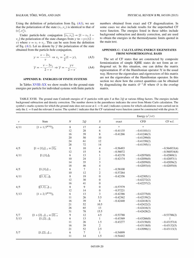
BALRAM, TOKE, WOJS, AND JAIN PHYSICAL REVIEW B 91, 045109 (2015)
Using the definition of polarization from Eq. (A1), we seethat the polarization of the state (ν↑,ν↓) is identical to that of(ν∗
↑,ν∗↓).
Under particle-hole conjugation [ν↑,ν↓] → [1 − ν↑,1 −ν↓] the polarization of the state changes from γ to −γ ν/(2 −ν) where ν = ν↑ + ν↓. This can be seen from the definitionof Eq. (A1). Let us denote by γ the polarization of the stateobtained from the particle-hole conjugation,
γ = ν − 2ν↓ν
⇒ ν↓ = ν
2(1 − γ ), (A3)
γ = −ν − 2ν↓2 − ν
⇒ γ = − γ ν
2 − ν. (A4)
APPENDIX B: ENERGIES OF FINITE SYSTEMS
In Tables XVIII–XX we show results for the ground-stateenergies per particle for individual systems with finite particle
numbers obtained from exact and CF diagonalization. Insome cases we also include results for the unperturbed CFwave function. The energies listed in these tables includebackground subtraction and density correction, and are usedto obtain the energies in the thermodynamic limits quoted inthe main text.
APPENDIX C: CALCULATING ENERGY EIGENSTATESFROM NONORTHOGONAL BASIS
The set of CF states that are constructed by compositefermionization of simple IQHE states do not form an or-thogonal set. In this situation, one can define the matrixrepresentation H of the Hamiltonian operator H in the usualway. However the eigenvalues and eigenvectors of this matrixare not the eigenvalues of the Hamiltonian operator. In thissection we show how the correct quantities can be obtainedby diagonalizing the matrix O−1H where O is the overlapmatrix.
TABLE XVIII. The ground state Coulomb energies of N particles with spin S at flux 2Q at various filling factors. The energies includebackground subtraction and density correction. The number shown in the parentheses indicates the error from Monte Carlo calculation. Thesymbol ∗ marks systems for which the ground state does not occur at L = 0; and ‡ indicates systems for which calculations were carried out inonly the L = 0 and the relevant S sector. The symbol † indicates that the CF variational wave function cannot be constructed with the given N .
Energy (e2/ε )
ν State N 2Q S exact CFD CF w.f.
4/11 [1 + 1/3WYQ]2 8 17 4 * *12 28 6 −0.41135 −0.41101(1)16 39 8 −0.41266 −0.41246(3)20 50 10 −0.41299(0)24 61 12 −0.41350(2)28 72 14 −0.41395(1)
4/5 [1 + [1]2]−2 ≡ [1]4 8 10 4 −0.56493 −0.564933(4)12 15 6 −0.56072 −0.560534(8)
4/11 [1,[1]2]2 6 13 1 −0.42170 −0.42070(0) −0.42069(1)10 24 2 −0.42174 −0.42056(0) −0.42057(1)14 35 3 −0.42059(0) −0.42056(2)18 46 4 −0.42053(4) −0.42055(8)
4/5 [1,[1]2]−2 6 7 1 −0.5810010 12 2 −0.57264
4/11 [[1,1]−2]2 8 19 0 −0.42356 −0.42305(1)12 30 0 −0.42272(2)16 41 0 −0.42257(2)
4/5 [[1,1]−2]−2 8 9 0 −0.5757912 14 0 −0.57221
5/13 [1 + 2/3WYQ]2 6 13 3 −0.42386 −0.42375(0)11 26 5.5 −0.42362 −0.42339(2)16 39 8 −0.42440 −0.42418(3)21 52 10.5 −0.42422(2)26 65 13 −0.42416(3)31 78 15.5 −0.42428(2)
5/7 [1 + [2]−2]−2 ≡ [2]−4 9 12 4.5 −0.53788 −0.53788(2)5/13 [1,[2]−2]2 6 13 1 −0.43369 −0.43266(0) †
11 26 1.5 −0.43277 −0.43156(0) −0.43157(4)16 39 2 −0.43118(0) −0.43132(5)21 52 2.5 −0.43096(1) −0.43113(3)
5/7 [1,[2]−2]−2 6 7 1 −0.5489911 14 1.5 −0.54442
045109-20

PHASE DIAGRAM OF FRACTIONAL QUANTUM HALL . . . PHYSICAL REVIEW B 91, 045109 (2015)
TABLE XIX. Same as Table XVIII.
Energy (e2/ε )
ν State N 2Q S exact CFD CF w.f.
7/19 [1 + [2]2]2 9 20 4.5 * *16 39 8 −0.41537 −0.41516(3)23 58 11.5 −0.41570(4)‡
7/9 [1 + [2]2]−2 ≡ [2]4 9 12 4.5 −0.56128 −0.56128(2)16 21 8 −0.55402 −0.55396(1)23 30 11.5 −0.55126 −0.551215(8)30 39 15 −0.54995 −0.549861(8)
7/19 [1,[2]2]2 ≡ [[3]−2]2 11 26 1.5 −0.42356 −0.42238(0) −0.42238(5)18 45 3 −0.42241(0)‡ −0.42243(4)25 64 4.5 −0.42262(4) −0.42244(4)
7/9 [1,[2]2]−2 ≡ [[3]−2]−2 11 14 1.5 −0.568107/19 [[1,2]−2]2 6 13 1 −0.42446 −0.42346(0)
13 32 1.5 −0.42365(0)20 51 2 −0.42411(8)
7/9 [[1,2]−2]−2 6 7 1 −0.572878/21 [1 + [3]−2]2 8 18 4 * *
16 39 8 −0.42237 −0.42216(3)24 60 12 −0.42188(2)‡
8/11 [1 + [3]−2]−2 ≡ [3]−4 8 10 4 −0.53864 †16 21 8 −0.53573 †
8/21 [1,[3]−2]2 ≡ [[2]2]2 10 24 2 −0.43166 −0.43046(0) †18 45 3 −0.42952(0)‡ †26 66 4 −0.42924(2)‡ −0.4292(1)
8/11 [1,[3]−2]−2 ≡ [[2]2]−2 10 12 2 −0.5460018 23 3
8/21 [[1,1]2]2 12 29 0 −0.43075(0)‡
20 50 0 −0.43003(2)‡
8/11 [[1,1]2]−2 12 15 0 −0.5489720 26 0
Let H be an operator which we intend to diagonalize withinthe space V spanned by the nonorthonormal set of vectors{|1〉 , |2〉 , |3〉 , . . . , |n〉}. The quantities H and O defined as
Hij = 〈i|H |j 〉 ,(C1)
Oij = 〈i| I |j 〉
are the quantities numerically computed through Monte Carlointegrations. I is the identity operator. Let |φ〉 and ε be aneigenvector and corresponding eigenvalue of H in the Hilbertspace V . By using the completeness relation, this eigenstatecan be expanded in the nonorthogonal basis.
|φ〉 =⎡⎣ n∑
i,j=1
|i〉 [O−1]ij 〈j |⎤⎦ |φ〉
=n∑
i=1
ci |i〉 where ci =n∑
j=1
[O−1]ij 〈j |φ〉 . (C2)
We prove below that the column vector containing the expan-sion coefficients ci is a right eigenvector of the non-Hermitianmatrix O−1H with an eigenvalue ε.
Since |φ〉 is an eigenstate, H |φ〉 = ε |φ〉. Inserting thecompleteness relations we get
[n∑
k,l=1
|k〉 [O−1]kl 〈l|]H
⎡⎣ n∑
i,j=1
|i〉 [O−1]ij 〈j |⎤⎦ |φ〉
= ε
[n∑
a,b=1
|a〉 [O−1]ab 〈b|]
|φ〉 .
After rearranging the summations and using the definition ofH and ci , the above equality can be rewritten as
n∑k=1
|k〉 [O−1Hc]k = ε
n∑k=1
ck |k〉 .
Since the basis vectors are linearly independent, this can betrue only if the coefficients of the vectors are equal on bothsides, which implies
O−1Hc = εc. (C3)
Every eigenvalue of the operator H in V is therefore aneigenvalue of matrix O−1H . The corresponding eigenvector ofthe matrix provides the coefficients for expanding the state in
045109-21

BALRAM, TOKE, WOJS, AND JAIN PHYSICAL REVIEW B 91, 045109 (2015)
TABLE XX. Same as Table XVIII.
Energy (e2/ε )
ν State N 2Q S exact CFD CF w.f.
10/27 [1 + [3]2]2 14 33 7 −0.41500 −0.41487(0)24 60 12 −0.41599(3)‡
10/13 [1 + [3]2]−2 ≡ [3]4 14 19 7 −0.55480 †24 32 12 −0.54972 −0.549679(7)34 45 17 −0.54774 −0.54766(1)
10/27 [1,[3]2]2 ≡ [[4]−2]2 6 12 0 −0.42391 −0.42336(0) †16 39 2 −0.42311(0) †26 66 4 −0.42323(3) −0.42317(4)
10/13 [1,[3]2]−2 ≡ [[4]−2]−2 6 8 0 −0.5817016 21 2 −0.56307
10/27 [[2,2]−2]2 12 29 0 −0.4247222 56 0
10/13 [[2,2]−2]−2 12 15 0 −0.5645911/29 [1 + [4]−2]2 12 29 6 −0.42243 −0.42219(0)
23 58 11.5 −0.42176(9)‡
11/15 [1 + [4]−2]−2 ≡ [4]−4 12 15 6 −0.53684 †23 30 11.5 −0.53527 †
11/29 [1,[4]−2]2 ≡ [[3]2]2 14 35 3 −0.42956(0) †25 64 4.5 −0.42882(2)‡ †
11/15 [1,[4]−2]−2 ≡ [[3]2]−2 14 17 3 −0.5452025 32 4.5
11/29 [[1,2]2]2 13 32 1.5 −0.42987(0)24 61 2
11/15 [[1,2]2]−2 13 16 1.5 −0.5485024 31 2
3/8 [1 + 1/2APf]2 6 13 3 −0.41852 −0.41844(0)12 29 6 −0.42002 −0.41978(5)18 45 9 −0.41953(1)24 61 12 −0.41991(2)
3/8 [1,1/2APf]2 8 19 2 −0.42914 −0.42833(0)14 35 3 −0.42711(0)20 51 4 −0.42669(2)26 67 5 −0.42640(0)
terms of the nonorthogonal basis. These eigenvalues exhaustall the possible eigenvalues of O−1H .
APPENDIX D: DOUBLE FQHEOF COMPOSITE FERMIONS
In this paper we have considered only the states in whichFQHE occurs in no more than one component of compositefermions. These are expected to be the most prominent FQHEstates of composite fermions. In this section we discuss thesimplest state which involves FQHE in two components ofcomposite fermions and also satisfies the Fock condition,namely the two-component 5/3 state formed as (1 + 1/3,1/3).[Note that a state of the type (1/3,1/3) does not satisfy the Fockcondition.]
The simplest possibility is [1 + [1]2,[1]2]2, in which wefill the spin-up lowest �L (L�L) completely and construct[1]2 state in the spin-up second �L and spin-down lowest �L.This gives us the following relations between the flux and the
number of particles in each �L:
2Q∗ + 1 = N0↑, (D1)
2Q∗ + 1 = 3N0↓ − 2, (D2)
2Q∗ + 3 = 3N1↑ − 2. (D3)
From the last two equations we obtain (N1↑ − N0↓) = 23 /∈ Z.
Therefore this state cannot be constructed. A similar argumentshows that the corresponding 5/3 state formed by 1/3 WYQstates in both spin-up second �L and spin-down L�L withspin-up L�L full cannot be constructed.
Next, we consider [1 + 1/3WYQ,[1]2]2, in which we fillthe spin-up L�L completely and construct 1/3WYQ and [1]2
states in the spin-up second �L and spin-down lowest �Lrespectively. This gives us the following set of relations:
2Q∗ + 1 = N0↑,
2Q∗ + 1 = 3N0↓ − 2,
045109-22

PHASE DIAGRAM OF FRACTIONAL QUANTUM HALL . . . PHYSICAL REVIEW B 91, 045109 (2015)
2Q∗ + 3 = 3N1↑ − 6,
N = N0↑ + N0↓ + N1↑,
N0↑ = 3k − 2,N0↓ = k,N1↑ = k + 2 (k ∈ N),
N = 5k, 2Q∗ = 3k − 3, S = 3k
2.
From this state at ν∗ = 5/3, we can construct states at ν =5/13 and ν = 5/7 (by reverse flux attachment). Doing exactdiagonalization at the corresponding flux, we find that thelowest-energy state does not have L = 0 for all allowed valuesof N and hence is unlikely to be incompressible.
The third possibility is [1 + [1]2,1/3WYQ]2, in which oneconstructs the 1/3WYQ state in the spin-down lowest �L and[1]2 in second �L. This implies the following relations:
2Q∗ + 1 = N0↑, (D4)
2Q∗ + 1 = 3N0↓ − 6, (D5)
2Q∗ + 3 = 3N1↑ − 2. (D6)
From the last two equations we find that (N1↑ − N0↓) = − 23 /∈
Z. Hence this state cannot be constructed.
APPENDIX E: SPIN SINGLET FQHE AT 4/11
In this section we provide details of the excitation spectrumof the 4/11 spin singlet state. The spectra of partially polarizedand fully polarized 4/11 states have been discussed previouslyin Refs. [47,48,50,51,77]. The 4/11 FQHE has been observedbut no spin phase transition has yet been observed. This alsoserves as an illustration of how we have obtained variousenergies by the method of CFD.
As stated above, the ν = 4/11 spin singlet state is obtainedfrom the ν∗ = 4/3 spin singlet state which is the particle-holeconjugate state to the 2/3 spin singlet. The 2/3 spin singletstate is obtained by filling the lowest �L of spin-up and spin-down completely and composite-fermionizing this state byreverse flux attachment. A straightforward calculation showsthat the spin singlet 4/11 state occurs at flux
2Q = 114 N − 3. (E1)
Therefore we must choose the particle number N to be amultiple of 4.Figure 6 shows the Coulomb spectra obtained from CFdiagonalization in the spherical geometry for three systems,namely N = 4, 8, and 12. The spectrum is obtained byconstructing all Sz = 0 and Lz = 0 states at 4/3 at theeffective flux 2Q∗ = 2Q − 2(N − 1), composite fermionizingthem by the standard method to obtain the CF basis at thedesired 2Q given by Eq. (E1), and then diagonalizing theCoulomb interaction in that subspace by the method of CFdiagonalization. (Here Sz and Lz are the z components ofthe total spin and orbital angular momentum.) For four andeight particles, we also display the exact spectrum (obtainedby a diagonalization of the Coulomb interaction in the fullLLL Hilbert space), and a comparison shows the accuracywith which the CF theory captures the low-energy physics. Inparticular, the ground state is seen to have S = 0 and L = 0,consistent with a a spin singlet FQHE state of composite
0 2 42.0
2.1
2.2
2.3
N = 4, 2Q = 8
Ener
gy(e
2/
)
L
S = 0 (CF)S = 0 (exact)S = 1 (CF)S = 1 (exact)
0 2 4 6 8
6.75
6.80
6.85
N = 82Q = 19
Ener
gy(e
2/
)L
S = 0 (CF)S = 0 (exact)S = 1 (CF)S = 1 (exact)S = 2 (CF)S = 2 (exact)
0 5 10 15
13.30
13.35
13.40
13.45
N = 122Q = 30
Ener
gy(e
2/
)
L
S = 0S = 1S = 2S = 3
0 2 413.27
13.28
13.29
N = 122Q = 30E
ner
gy(e
2/
)
L
charge excitonspin-flip exciton
FIG. 6. (Color online) Energy spectrum of the 4/11 spin singletFQHE state, where composite fermions form a spin singlet 4/3 FQHEstate. The spectra shown by dots (different colors representing differ-ent spin quantum numbers S) were obtained by CF diagonalization.The dashes in the top two panels show the exact spectrum obtained byexact diagonalization in the full Hilbert space. The spherical geometryis used for the calculation. L is the total orbital angular momentum,2Q is the flux through the sphere in units of the flux quantum, andN is the total number of electrons. The bottom panel shows the twolowest-energy collective modes, namely the charge exciton and thespin-flip exciton.
045109-23

BALRAM, TOKE, WOJS, AND JAIN PHYSICAL REVIEW B 91, 045109 (2015)
fermions here. The thermodynamic limit of the ground-stateenergy per particle is obtained by an extrapolation of the threeenergies. We find that even with two points (with four andeight particles) we get a reasonably good approximation forthe ground-state energy, which is why we have used for somestates that involve reverse flux attachment the exact energiesonly from two systems to obtain the thermodynamic energy.
It is interesting to ask if we can make quantitativepredictions about the nature of the charge and spin collectivemodes at 4/11. As known from previous studies [78,79],the collective modes are excitons of composite fermions thatinvolve either a spin flip or no spin flip, called spin-flip excitonsor charge excitons, respectively. They can be constructed upto a maximum L in the spherical geometry. The CF theorypredicts this value as follows. The 12-particle 4/11 state mapsinto the 12-particle 4/3 state at flux 2Q∗ = 8, which, byparticle-hole symmetry, is equivalent to a six-particle spinsinglet 2/3 state at 2Q∗ = 8. This state, in turn, maps into
a six-particle spin singlet state at filling factor 2. The lowest-energy CF exciton of the spin singlet 4/11 state is thus derivedfrom the lowest-energy exciton of the six-particle ν∗∗ = 2 stateat flux 2|Q∗∗| = 2. The latter exciton corresponds to a particlewith angular momentum 2 and a hole with angular momentum1, giving a spin polarized exciton at L = 2,3 (L = 1 excitonis annihilated [78,80]) and a spin-flip exciton at L = 1,2,3.This shows that larger systems would be required for bringingout the full nature of the excitonic collective-mode dispersion.Nonetheless, from the spectra, it is clear that both the chargeand the spin-flip exciton modes are gapped, as expected for aspin singlet FQHE state, and that both of them have at least oneroton minimum. Rotons in the charge mode were first predictedby Girvin, MacDonald, and Platzman [81] and spin-flip rotonshave also been predicted [55] and observed [58] for fully spinpolarized 2/5 and 3/7. We note that the roton gaps for the spinsinglet 4/11 are on the order of 0.01e2/ε for both charge andspin-flip exciton modes.
[1] D. C. Tsui, H. L. Stormer, and A. C. Gossard, Phys. Rev. Lett.48, 1559 (1982).
[2] J. P. Eisenstein, H. L. Stormer, L. Pfeiffer, and K. W. West, Phys.Rev. Lett. 62, 1540 (1989).
[3] R. R. Du, A. S. Yeh, H. L. Stormer, D. C. Tsui, L. N. Pfeiffer,and K. W. West, Phys. Rev. Lett. 75, 3926 (1995).
[4] I. V. Kukushkin, K. v. Klitzing, and K. Eberl, Phys. Rev. Lett.82, 3665 (1999).
[5] I. V. Kukushkin, J. H. Smet, K. von Klitzing, and K. Eberl, Phys.Rev. Lett. 85, 3688 (2000).
[6] S. Melinte, N. Freytag, M. Horvatic, C. Berthier, L. P. Levy,V. Bayot, and M. Shayegan, Phys. Rev. Lett. 84, 354 (2000).
[7] L. Tiemann, G. Gamez, N. Kumada, and K. Muraki, Science335, 828 (2012).
[8] A. S. Yeh, H. L. Stormer, D. C. Tsui, L. N. Pfeiffer, K. W.Baldwin, and K. W. West, Phys. Rev. Lett. 82, 592 (1999).
[9] Y. Liu, D. Kamburov, S. Hasdemir, M. Shayegan, L. N. Pfeiffer,K. W. West, and K. W. Baldwin, Phys. Rev. Lett. 113, 246803(2014).
[10] X. Du, I. Skachko, F. Duerr, A. Luican, and E. Y. Andrei, Nature(London) 462, 192 (2009).
[11] K. Bolotin, F. Ghahari, M. D. Shulman, H. Stormer, and P. Kim,Nature (London) 462, 196 (2009).
[12] C. R. Dean, A. F. Young, P. Cadden-Zimansky, L. Wang, H. Ren,K. Watanabe, T. Taniguchi, P. Kim, J. Hone, and K. L. Shepard,Nat. Phys. 7, 693 (2011).
[13] B. E. Feldman, B. Krauss, J. H. Smet, and A. Yacoby, Science337, 1196 (2012).
[14] B. E. Feldman, A. J. Levin, B. Krauss, D. A. Abanin, B. I.Halperin, J. H. Smet, and A. Yacoby, Phys. Rev. Lett. 111,076802 (2013).
[15] F. Amet, A. J. Bestwick, J. R. Williams, L. Balicas, K. Watanabe,T. Taniguchi, and D. Goldhaber-Gordon, arXiv:1410.3549[cond-mat].
[16] N. C. Bishop, M. Padmanabhan, K. Vakili, Y. P. Shkolnikov,E. P. De Poortere, and M. Shayegan, Phys. Rev. Lett. 98, 266404(2007).
[17] M. Padmanabhan, T. Gokmen, and M. Shayegan, Phys. Rev. B80, 035423 (2009).
[18] T. M. Kott, B. Hu, S. H. Brown, and B. E. Kane, Phys. Rev. B89, 041107 (2014).
[19] J. Shabani, Y. Liu, and M. Shayegan, Phys. Rev. Lett. 105,246805 (2010).
[20] J. K. Jain, Phys. Rev. Lett. 63, 199 (1989).[21] A. Lopez and E. Fradkin, Phys. Rev. B 44, 5246 (1991).[22] B. I. Halperin, P. A. Lee, and N. Read, Phys. Rev. B 47, 7312
(1993).[23] J. K. Jain, Composite Fermions (Cambridge University Press,
New York, 2007).[24] Composite Fermions: A Unified View of the Quantum Hall
Regime, edited by O. Heinonen (World Scientific, Singapore,1998).
[25] J. K. Jain and R. K. Kamilla, in Composite Fermions (WorldScientific, Singapore, 1998), Chap. 1, pp. 1–90.
[26] A. Lopez and E. Fradkin, in Composite Fermions (Ref. [25]),Chap. 3, pp. 195–253.
[27] S. H. Simon, in Composite Fermions (Ref. [25]), Chap. 2,pp. 91–194.
[28] Perspectives in Quantum Hall Effects, edited by S. Das Sarmaand A. Pinczuk (Wiley–VCH Verlag GmbH, New York, 2007).
[29] B. I. Halperin, in Perspectives in Quantum Hall Effects(Ref. [28]), pp. 225–263.
[30] H. L. Stormer, in Perspectives in Quantum Hall Effects(Ref. [28]), pp. 385–421.
[31] J. K. Jain, Phys. Today 53(4), 39 (2000).[32] B. I. Halperin, Physica E 20, 71 (2003).[33] J. H. Smet, K. von Klitzing, D. Weiss, and W. Wegscheider,
Phys. Rev. Lett. 80, 4538 (1998).[34] G. Murthy and R. Shankar, Rev. Mod. Phys. 75, 1101 (2003).[35] X. G. Wu, G. Dev, and J. K. Jain, Phys. Rev. Lett. 71, 153 (1993).[36] K. Park and J. K. Jain, Phys. Rev. Lett. 80, 4237 (1998).[37] K. Park, V. Melik-Alaverdian, N. E. Bonesteel, and J. K. Jain,
Phys. Rev. B 58, R10167 (1998).[38] K. Park and J. K. Jain, Phys. Rev. Lett. 83, 5543 (1999).[39] K. Park and J. K. Jain, Solid State Commun. 119, 291 (2001).[40] S. C. Davenport and S. H. Simon, Phys. Rev. B 85, 245303
(2012).[41] C. Toke and J. K. Jain, Phys. Rev. B 75, 245440 (2007).
045109-24

PHASE DIAGRAM OF FRACTIONAL QUANTUM HALL . . . PHYSICAL REVIEW B 91, 045109 (2015)
[42] C. Toke and J. K. Jain, Phys. Rev. B 76, 081403 (2007).[43] M. O. Goerbig and N. Regnault, Phys. Rev. B 75, 241405 (2007).[44] I. Sodemann and A. H. MacDonald, Phys. Rev. Lett. 112, 126804
(2014).[45] D. A. Abanin, B. E. Feldman, A. Yacoby, and B. I. Halperin,
Phys. Rev. B 88, 115407 (2013).[46] W. Pan, H. L. Stormer, D. C. Tsui, L. N. Pfeiffer, K. W. Baldwin,
and K. W. West, Phys. Rev. Lett. 90, 016801 (2003).[47] A. Wojs, K.-S. Yi, and J. J. Quinn, Phys. Rev. B 69, 205322
(2004).[48] S. Mukherjee, S. S. Mandal, Y.-H. Wu, A. Wojs, and J. K. Jain,
Phys. Rev. Lett. 112, 016801 (2014).[49] K. Park and J. K. Jain, Phys. Rev. B 62, R13274 (2000).[50] C.-C. Chang, S. S. Mandal, and J. K. Jain, Phys. Rev. B 67,
121305 (2003).[51] A. Wojs, G. Simion, and J. J. Quinn, Phys. Rev. B 75, 155318
(2007).[52] Y. Liu, S. Hasdemir, A. Wojs, J. K. Jain, L. N. Pfeiffer,
K. W. West, K. W. Baldwin, and M. Shayegan, Phys. Rev. B90, 085301 (2014).
[53] A. C. Balram, U. Wurstbauer, A. Wojs, A. Pinczuk, and J. K.Jain, arXiv:1406.4042 [cond-mat].
[54] Y. Liu and M. Shayegan (private communication).[55] S. S. Mandal and J. K. Jain, Phys. Rev. B 63, 201310 (2001).[56] D. Mujumder, S. Mandal, and J. Jain, Nat. Phys. 5, 403
(2009).[57] T. D. Rhone, D. Majumder, B. S. Dennis, C. Hirjibehedin,
I. Dujovne, J. G. Groshaus, Y. Gallais, J. K. Jain, S. S. Mandal,A. Pinczuk et al., Phys. Rev. Lett. 106, 096803 (2011).
[58] U. Wurstbauer, D. Majumder, S. S. Mandal, I. Dujovne, T. D.Rhone, B. S. Dennis, A. F. Rigosi, J. K. Jain, A. Pinczuk, K. W.West et al., Phys. Rev. Lett. 107, 066804 (2011).
[59] C. Toke and J. K. Jain, J. Phys.: Condens. Matter 24, 235601(2012).
[60] D. Majumder and S. S. Mandal, Phys. Rev. B 90, 155310(2014).
[61] M. Hamermesh, Group Theory and Its Application to PhysicalProblems (Dover, New York, 1962).
[62] J. K. Jain and R. K. Kamilla, Int. J. Mod. Phys. B 11, 2621(1997).
[63] J. K. Jain and R. K. Kamilla, Phys. Rev. B 55, R4895 (1997).[64] R. B. Laughlin, Phys. Rev. Lett. 50, 1395 (1983).[65] B. I. Halperin, Helv. Phys. Acta 56, 75 (1983).[66] G. Moore and N. Read, Nucl. Phys. B 360, 362 (1991).[67] M. Levin, B. I. Halperin, and B. Rosenow, Phys. Rev. Lett. 99,
236806 (2007).[68] S.-S. Lee, S. Ryu, C. Nayak, and M. P. A. Fisher, Phys. Rev.
Lett. 99, 236807 (2007).[69] C. Toke, P. E. Lammert, V. H. Crespi, and J. K. Jain, Phys. Rev.
B 74, 235417 (2006).[70] S. Mukherjee, S. S. Mandal, A. Wojs, and J. K. Jain, Phys. Rev.
Lett. 109, 256801 (2012).[71] S. Mukherjee, J. K. Jain, and S. S. Mandal, Phys. Rev. B 90,
121305 (2014).[72] S. S. Mandal and J. K. Jain, Phys. Rev. B 66, 155302 (2002).[73] F. D. M. Haldane, Phys. Rev. Lett. 51, 605 (1983).[74] R. Morf, N. d’Ambrumenil, and B. I. Halperin, Phys. Rev. B 34,
3037 (1986).[75] W. Pan, K. W. Baldwin, K. W. West, L. N. Pfeiffer, and D. C.
Tsui, Phys. Rev. B 91, 041301 (2015).[76] N. Samkharadze, I. Arnold, L. N. Pfeiffer, K. W. West, and
G. A. Csathy, arXiv:1412.8186; N. Samkharadze, Ph.D. thesis,Purdue University, 2013.
[77] S. Mukherjee, S. S. Mandal, Y.-H. Wu, A. Wojs, and J. K. Jain,Phys. Rev. Lett. 112, 199902(E) (2014).
[78] G. Dev and J. K. Jain, Phys. Rev. Lett. 69, 2843 (1992).[79] V. W. Scarola, K. Park, and J. K. Jain, Phys. Rev. B 61, 13064
(2000).[80] S. He, S. H. Simon, and B. I. Halperin, Phys. Rev. B 50, 1823
(1994).[81] S. M. Girvin, A. H. MacDonald, and P. M. Platzman, Phys. Rev.
Lett. 54, 581 (1985).
045109-25