1

PHD PROGRAMME IN ISTITUTIONS AND

POLICIES

ciclo XXVI

S.S.D: SECS P/02 POLITICA ECONOMICA

SECS-P/06 ECONOMIA APPLICATA

TITOLO TESI:

AN EMPIRICAL INVESTIGATION OF THE

COMMON AGRICULTURAL POLICY

REFORM PROCESS

Coordinatore: Ch.mo Prof. PAOLO COLOMBO

Tesi di Dottorato di : FINO CARLO

Matricola: 3911217

Anno Accademico: 2013/2014

2

Index

Introduction pag. 3

Acknowledgements pag. 10

Part I. The old common agricultural policy pag. 11

The origin of the CAP as a price support policy pag. 14

The functioning of a price support policy in a food importing country and the rationale

behind the adoption of a price support policy in Europe pag. 35

The farm income problem pag. 43

The functioning of a price support policy in a food exporting country pag. 62

The “three crisis” and the necessity of a structural reform of the CAP pag. 85

Part II. The reform process: An empirical investigation of the Mac Sharry and Fischler’s

reforms pag. 94

Introduction pag. 104

Data description and methodology pag. 112

Empirical results and analysis pag. 121

Conclusions pag. 171

Part III. Perspectives of reform. pag. 174

Conclusions pag. 208

Bibliography pag. 211

3

Introduction.

This research is an attempt to carry out an extensive analysis of the evolution

of the European Common Agricultural Policy and its relations with the

European agricultural sector. The specific focus is on the impacts of the set

of reforms that occurred in the last twenty years, starting with the first

attempts of reforms of the eighties and culminating with the structural

reforms of 1992, 1999 and 2003.1

Intuitively, the history of the Common Agricultural Policy is a wide topic

and a more specific definition of the goal of the present research is

necessary. To start narrowing the topic, I will analyse the evolution of the

regulations regarding the cereal sector which can be considered emblematic

for the CAP overall; in fact, the set of reforms that was first applied to cereal

has been extended to other agricultural sectors, following the same logic of

switching from a price support policy to a system based on direct payments

to farmers, progressively decoupled from production decisions. I will

reconstruct the economic and political context that lead to the reform

process, highlighting its main drivers. Most of all, I will provide a

quantitative analysis of the effects of the two main reforms (Mac Sharry and

1 Namely, Mac Sharry, Agenda 2000 and Fischler’s reforms. Anyway, the empirical tests in

part two are carried out only on the first and the latter, assuming Agenda 200 did not

introduce nothing revolutionary but rather reinforced already existing instruments, at

least for the matter under consideration. The idea is that is Mac Sharry introduced direct

payments in place of price support and Fischler’s reform decoupled them from

production, Agenda 2000 just reinforced the cut in intervention prices already started in

1992.

4

Fischler) to verify whether they had the expected impacts in terms of

reduction of the overall cereal production and a reduction in the greenhouse

gas emissions from the agricultural sector. Finally, I will comment on the

effectiveness of the reform process; this will be particularly useful since a

new proposal of reform for the period post 2013 is being negotiated at the

moment, with the main aim of reforming the single payment scheme

introduced by the Fischler reform.

The organisation of the present work is in three parts: an historic description

of the ‘old’ CAP and the drivers for the reforms; an empirical analysis of the

reform process and a discussion about the current reform proposal for the

post 2013 period and its likely effects on farming practices and farmers’

income.

In the first part I reconstruct the history of the CAP, its birth and the reasons

for its initial articulation as a price support policy. Most importantly, this

section is crucial to explain the drivers that lead to the necessity of

implementing a structural reform of the CAP. I will identify two sets of

drivers of the reform process, in accordance with the existing literature

(Cuhna, 2012; Baldwin, 2003)2: internal and international. Among the first

set, budgetary pressures due to the functioning of the price support

mechanism and society’s demands for a reduction in the environmental

impacts of agriculture and for a higher quality food at reasonable prices were

the main political pressures for a reform. Regarding the international

2 A. Cunha and A. Swinbank, (2012) “An inside view of the CAP reform process”, Oxford

University Press. R. Baldwin and C. Wiplosz, (2003) “The Economics of European Integration”, Mac Graw-Hill, 3

rd edit.

5

pressures, starting from the Uruguay round of the GATT in the eighties, food

exporting countries (the CRAINS group and the US) called for the

introduction of agriculture among the sectors to be progressively liberalised,

adding another reason to reform the existing set of policies.

This first part consists in a detailed literature review about the distortions

and limits of the ‘old’ CAP and it is instrumental to provide a clear

description of the context of the reform process. Its main goal is to show

how what I define as “three crises” (budgetary, environmental, trade

relations) were the direct consequence of a system that for its very nature

created perverse mechanism that determined overproduction, pressures on

the environment and downward pressures on international prices with

consequent trade distortions. It defines the context that lead to the reform

process started, as regards the cereal sector, with the Mac Sharry reform in

1992 and then continued with Agenda 2000 in 1999, the Fischler reform of

2003, the so-called Health Check of 2008 and the reform that has recently

been negotiated and that would take place for the period post 2013.

The second part builds on the results drawn in the first part and analyses the

effectiveness of the reform process occurred in the last twenty years. In order

to do that I run an econometric model using the difference in difference

technique to test, in particular, the effects of the two reforms that are almost

universally considered to be the turning points of the CAP (please note that I

refer to the cereal sector as it can be considered emblematic for the reform

process overall): the Mac Sharry reform and the Fischler reform. The reason

for this choice is that these two reforms mark two deep discontinuities in the

CAP functioning. The Mac Sharry reform replaces the price support system

6

with direct payments per hectare, decoupling payments from (the level of)

production. However, these payments were still coupled to the type of

commodity cropped: it was a direct payment per hectare for the land

currently cultivated with cereal and therefore they were still partially

distortionary on production decisions. In fact, when other sectors were

progressively reformed in a similar way,3 the problem of different levels of

payment per hectare depending on the type of crop shows clearly how these

payment, although able to end the incentive to maximize the level of

productions that characterized the old price support mechanism, still created

distortions regarding production decisions: the farmer, knowing he would

receive different EU payments per hectare depending on the crop cultivated,

still did not make production decisions based just on (liberalized) market

prices but also looking at the different levels of support per hectare offered

by the Agricultural Policy. Hence, also Mac Sharry direct payments were

still partially distortionary.4

The Fischler reform completed the process, introducing a single payment

scheme (SPS) that is considered to be almost fully decoupled (doubts persist,

among academics and policy-makers, over the role of the cross compliance

3 This is what happened after Agenda 2000, which extended the principles of Mac

Sharry’s reforms to other commodities. Being a direct payment per hectare based on the

commodity cropped at the moment, we can model it as different premiums for different

products. Hence, even if this subsidy was not linked anymore with the level of

production, it was still linked with the type of production. 4 In the second part of the research I will run an econometric test to see whether farmers

started taking production decisions based on international rather than on intervention

prices. Here, I can anticipate that, even if the sign on prices is unexpected (possibly

suggesting a Cobweb model for production decisions), international prices become

significant just after the Fischler reform, as the theory predicted.

7

requirements)5. Both in the “historic”, in the “hybrid” or in the “regional”

specifications of the Single Payment Scheme, in fact, production decisions

should not be affected anymore by the direct payments since the payments

are now either some flat rate per hectare for all the crops in a certain region

(regional model) or based on past payments (historic model) but anyway de-

linked by the current production decisions. In fact, to anticipate some of the

concepts that will be examined in detail in the second part, even in the most

conservative scenario (historic) the payments are provided based on the ones

received in a base period (2000-2002) and therefore are completely

decoupled from the current production decisions. It does not matter what the

farmer is producing now on its land. The amount of subsidy he receives on a

particular hectare is calculated depending on what he did in the reference

period. Hence those payments can be thought as lump sum transfers.

Coming to the methodology, I chose to run a difference in difference model

because, allowing for the presence of a control group, it can be used to

isolate the impacts of the reforms that occurred in the EU and not in the

other countries that constitute the control group. In practice, the presence of

both a treatment and a control group allows to control for other variables that

might have altered the trends in both groups, therefore isolating the effect of

the reform under consideration. The idea is that if a series of regressors with

potentially explanatory power are included both for the control and the

treatment group and there is still a difference in their trend in concomitance

5 The question whether these payments are still partially coupled with production moves

from the idea that if, in order to receive the payments, the farmer has to produce

something, these subsidies would still contribute boosting production beyond what

would be the optimal in a free market scenario.

8

of the reform, that residual (which would be captured by the coefficient on

the interaction term of my model) is the effect of the reform.

As an example suitable to the present case, let’s have a quick look at what

could happen if we tried to infer whether there was a reduction in emissions

in the EU, due to the change in policy, just looking at EU data. In fact, it

could be that a reduction in GHG emissions is due to an increase in fertilizer

prices that lead producer to decrease input use due to budget constrains; if

we just consider EU countries we might end up saying that the reduction in

emission is due to the reform (that happened to be contemporary to the

increase in fertilisers’ prices). The inclusion of a control group aims at

avoiding this type of mistake. In fact, in this case the reduction would appear

also in the control group. Hence, we would not misinterpret any

reduction/increment in the trend of the treatment group as a consequence of

the reform: just the residual, the coefficient on the interaction term, would in

fact capture the effects of the reforms. Just after having controlled for

explanatory variables that could have altered the trends “besides” the effect

of the reform (hence not only in the treatment but also in the control group),

we can make sure that the difference between treatment and control group,

pre and post, is the real reforms’ effect.

The tests on production and emissions are then followed by a robustness

check that I used to verify whether these two reforms lead farmers to take

production decisions on the basis of international rather that administratively

set intervention prices. Here, I anticipate that as expected this seems to

happen after the implementation of the SPS with the Fischler reform,

confirming the idea that Mac Sharry payments were still partially coupled

9

with the type of production and that Fischler reform succeeded in finalising

the process of liberalisation of European agriculture.

The third part completes the research, expanding on the results obtained in

the second part. In particular, I will comment on the effectiveness of the

reforms occurred to date and on the likely effects of the reform negotiated in

2013. In this context, it is important to consider the actual reform proposals

for the post 2013 and in particular the proposals regarding the reform of the

single payment scheme. The main goal of this third part is to establish the

likely effect of the recent reform both in terms of changes in agricultural

practices and in terms of its effects on farmers’ income: in particular I will

try to establish whether the increased share of first pillar payments that is

now conditional on the compliance to agro-environmental practices is the

right method to improve farming practices and if it is the most efficient way

to achieve this result in terms of pressures on the European budget and

effects on farmers’ income. Differently from the econometric test run in the

second part, the analysis carried out in this final part is mainly preliminary,

not based on data but rather on some reasonable predictions of the effects

that could be expected from a reform of the direct payments as the one that

has recently been approved.

10

Acknowledgements.

I would like to thank my PhD supervisors, Professors Fausta Pellizzari and

Mario A. Maggioni, for the help and the stimulus throughout the research.

The definition of the topic and the identification of a specific set of reforms

in a particular sector (cereal) was a necessary step to take in order to study

an otherwise too wide topic. Moreover, the current format of the research,

especially the third part with the analysis of the current reform proposal and

some suggestions of potential instruments to adopt, has been decided

together and I think it helps clarifying the future perspectives of this

fundamental European policy. I also would like to thank my MSc.

supervisor, professor Ben Lockwood (University of Warwick), for the

support received with the empirical part of the research and the elaboration

of the reduced form model; moreover, I owe a particular mention to Federica

Liberini (PhD at the University of Warwick) who gave me useful insights

regarding panel data analysis and the use of STATA. I hope I was able to get

the best from their advices and any mistake is a responsibility of the writer.

Last but not least, I would like to thank the Economic Department of the

Faculty of Social Science, in particular professor Guido Merzoni, for the

support received regarding the statistical tools used to carry out the empirical

part of the research.

11

PART I.

THE “OLD” COMMON AGRICULTURAL POLICY: ORIGINS AND

EVOLUTION OF THE CAP AS A PRICE SUPPORT POLICY AND

THE DRIVERS OF THE REFORM PROCESS.

As anticipated in the introduction, this part of the research is dedicated to an

extensive analysis of the so-called old Common Agricultural Policy and it is

functional to describe the context that drove to the need of an overall reform.

The outline is the following. First, I will provide an historic reconstruction of

the origin of the CAP in the late fifties, highlighting the economic, historical

(and also political) reasons that lead to the adoption of a price support policy

as the main tool of the new born Common Agricultural Policy.

Then, I will describe the functioning of the ‘old’ CAP in the context of a

food importing country, as the European Union happened to be for most of

the agricultural commodities in its early years. Since it might not appear

automatic that the agricultural sector has to be partially subsidised,6 I will

take a step back to analyse a standard argument in the agricultural literature,

the so-called ‘farm income problem’. This argument is normally used to

justify State intervention in the agricultural sector: if the ‘treadmill’

6 In fact, the major critique to the CAP by international competitors was to alter

international trade and distort the markets.

12

(Cochrane, 1958)7 description of the farm problem is accurate, State

intervention might have a justification as long as it is finalised to sustain

farm incomes, structurally declining in the aforementioned model; or, at

least, the rural exodus process that follows should be managed by some

forms of intervention and the minimum level of people to be employed in

agriculture should be established considering also social and environmental

factors.

Besides the validity of the ‘farm income’ argument, it is important to

consider whether a price support policy would be optimal to achieve the goal

of sustaining farmers’ income; in this context, it is useful to note Josling’s

(1969)8 consideration about the limits of a policy that used a single

instrument (the price support) to achieve a plural set of goals. Josling’s

thesis will be crucial for my critique of the price support mechanism as a

tool to achieve different goals such as sustaining farmers’ income and

achieve technical progress in the sector and will be used throughout the

present research. Indeed, the author considered the price support as

inadequate since for its nature it could not have been effective in achieving

different goals such as protecting farm incomes and the environment: as an

example, in this specific case, Josling highlighted that if price support might

have some benefits in terms of income support, its very conception would

have been incompatible with the goal of protecting the environment.

7 W. Cochrane, (1958) “Farm prices: myths and reality”, Minnesota University Press.

8 T. Josling “A formal approach to Agricultural Policy” in “Journal of Agricultural

Economics”, Volume 20, Issue 2, pages 175–196, May 1969

13

Having clarified the origins of the CAP as a price support policy I will then

move to describe its functioning when Europe became a food exporting

country. This switch from an importing to an exporting country can be

considered the beginning of the end of the old CAP and I will briefly analyse

some of the attempts taken by the European Commission to reform the

policy.

Together with the switch from being a food importer to a food exporter, I

will then focus on some internal mechanism that exacerbated the European

budgetary problems. I will focus in particular on the so called green money

system, the compromise of Luxemburg and the first decisions on common

prices as the main additional drivers to the budget crisis that affected the

CAP from the 70ies onwards and that were at the basis of the need to

attempt an overall reform of the policy.

The content of the reform proposal known as Mansholt plan will be quickly

outlined together with the reasons of its failure; moreover, I will present

some of the reforms undertaken during the 80ies, mainly not in the cereal

sector, to show how they were still ineffective to solve the problems related

to a policy based on a price support system.

Finally, it will be shown that the price support system itself, in a context of a

progressively more productive agriculture, was the real underlying reason of

the three crisis that the European Union was facing regarding its agricultural

sector: budgetary, environmental and trade relations.

14

1.1 The origin of the CAP as a price support policy.

In order to reconstruct the historical origin of the CAP and the reasons for its

implementation as a price support policy, the contributions of Zobbe (2000)9

and Fearne (1997)10

are particularly useful. Zobbe’s paper, in particular,

aims at providing some reasons for the choice of a price support mechanism

as the central instrument of what is called the old CAP, focusing on the

economic reasons. Fearne’s contribution, instead, helps contextualizing the

adoption of price support in the historical context of the European

Community post II World War. In the following paragraph, I will largely

rely on Fearne’s reconstruction of the years that preceded the birth of the

European Community and the CAP; also, O’ Rourke’s model will be used to

show the reason of the common inheritance of agricultural policies of the

first EU members.

9 H. Zobbe (2000) “The Economic and Historical Foundation of the Common Agricultural

Policy in Europe”, Fourth European Historical Economics Society Conference, September

2001. Merton College, Oxford, U.K.

10

A. Fearne, “The History and Development of the CAP 1945-1990”, in C. Ritson and D.R.

Harvey, “The Common Agricultural Policy”, 1997, CAB international, Wallingford, UK.

15

The historical roots of the Common Agricultural Policy.

As Fearne states, when examining the factors that determined the shape of

the CAP in the early 60ies, it is important to contextualize the analysis in the

broader process of European integration, aimed at creating an economic and

a political union.

European integration was thought to be a necessary step to guarantee peace

on the European continent and economic recovery after the II world war.

The signing of the Treaty of Brussels in 1948 can be considered the start of a

process that saw European countries negotiating the terms of their

participation in a supranational organisation in which they would have to

surrender parts of their sovereignty. In 1949 the Council of Europe was

created. In this context, the French proposed the creation of an European

parliamentary assembly in which decisions would be carried by majority

voting, implying a federal conception of the integration process. The

differences with the British approach to European integration were soon

clear, as the British succeeded in watering down the project conferring no

legislative powers to the Assembly and the Council. The Council then set up

a special Committee to analyse the prospects for the integration of European

agriculture in 1950.

16

France was particularly keen to create a common agricultural market,11

seeing it as part of a bargaining where Germany would have opened its

market to French produce in exchange of the liberalization of the industrial

sector that would have favoured Germany, and proposed to create an high

authority for agriculture with substantial supranational powers. The idea was

to control production, to establish a common market based on the removal of

all barriers to agricultural trade within Europe via a price support policy and

the use of import levies against non-European products. Contrasts with the

UK due the British denial of surrendering substantial parts of sovereignty

determined the failure to reach any agreement in the negotiations between

1952 and 1954.

An important step towards European integration was the creation, in 1951,

of the European Coal and Steel Community, formed by Benelux countries

and France, this time together with Italy and Germany, while Britain did not

participate. This plan, designed by Jean Monnet, made clear that due to the

difficulties to reach an agreement on a more ambitious political Union, the

method of integration followed by the European countries would have been

the so called “gradualist integration”, where the political goals had to be

reached progressively through a process of economic integration and

cooperation. In particular, Monnet thought that aiming at a sort of top-down

approach starting with the implementation of a political Union that would

have been similar to the construction of a new federal State, European’s

integration should have followed a more gradualist approach where each

11

See also W. Grant, “The Common Agricultural Policy”, 1997, The European Union

Series, Palgrave MacMillan. Chapter 3 for a detailed description of the CAP as a

compromise between France and Germany.

17

area of cooperation would have been analysed separately, depending on the

needs of the members in that particular area.

Aware of the difficulties to reach an agreement on a political union, the

Benelux countries outlined a series of proposals aimed at implementing the

“gradualist integration” method on a broader scale to create a fully integrated

European market. They presented a memorandum that called for an

intergovernmental conference which took place in Messina in June 1955

between the Six (Benelux countries plus France, Germany and Italy) but

without a disinterested Britain. The aim of the conference was to negotiate a

series of treaties that would have established a general common market. The

result of that conference was the “Spaak report”, drawn up in 1956, that

constituted the basis of the future Treaty of Rome, 1957, which formally

founded the European Economic Community (EEC). After the publication of

the Spaak report, a steering Committee started working on the different

sectors included in the unification process. Britain participated initially but

soon left the negotiations, easing the publication of the steering group

proposals which included agriculture among the sectors to be integrated in

the Common market.

The Spaak report outlined the objectives for the future agricultural policy,

contributing to define four of the goals which will be part of the Treaty of

Rome a year later:

- stabilization of markets;

- security of supply;

- sustain farm incomes;

18

- a gradual structural adjustment with an increase in farm productivity

and average size.

However, details regarding the policy to be implemented for the agricultural

sector were absent since the negotiations were still problematic between the

Six countries; moreover, agriculture was not considered a priority during the

negotiations on the Treaty that institutes the European Economic

Community.

For those reasons, the Treaty of Rome defines the main goal for the

agricultural sector without specifying the details about how to implement

them. These broad goals are described in the articles (38-49). In particular,

art. 39.1 defines the five main objectives of the policy:

(a) to increase agricultural productivity by promoting technical progress and

by ensuring the rational development of agricultural production and the

optimum utilization of the factors of production, in particular labour;

(b) thus to ensure a fair standard of living for the agricultural community, in

particular by increasing the individual earnings of persons engaged in

agriculture;

(c) to stabilize markets;

(d) to assure the availability of supplies;

(e) to ensure that supplies reach consumers at reasonable prices.

Art. 40 provides some reference to the policy options, mentioning the

necessity to form an internal common market and a common trade policy

with the external partners. Some instruments as regulated prices, production

19

aids and other market intervention mechanisms were outlined as potential

tools of the future agricultural policy.

Art 43 established the procedure to be followed to reach an agreement on the

CAP. The Commission was required to submit proposals to the Council

within three years and the Council would implement them with regulations,

directives and proposals.

As established by article 43, delegations from each member State, the main

farming organizations, the food industry and the Commission met in Stresa,

in July 1958, to agree on a more detailed view of the forthcoming CAP. In

this contest, a price support policy was advocated by different governments

even if the Commission and especially the Commissioner Sicco Mansholt

stressed that a price policy combined with a structural policy to increase

productivity could determine overproduction and therefore surpluses that

might worsen trade relations with EC’s trading partners, put pressure on the

European budget and endanger the economic sustainability of the policy

(Commission, 1958; Commission 1958a)12

. The farming representatives, in

particular, endorsed a price support policy as a tool to help the family farm,

that should remain the backbone of the European Agricultural sector. The

question whether this was the most appropriate tool is not answered here but

left for the next chapter, where I specifically question if this was an efficient

instrument to reach that goal. Here it is rather important to note that the

shared goal of sustaining a type of farm system based on small, family

12

Commission of the European Communities (1958), “First General Report on the

Activities of the Community, Brussels.

Commission of the European Communities (1958a), “Recuil des documents de la

conference agricole des etats members de la communaute economique europeenne a

Stresa au 12 Juillet 1958 ", Brussels.

20

owned business lead to the adoption of a policy based on the instrument of

common internal prices higher than the international ones for historical (and

at least at the very beginning economic) reasons.

After the Stresa conference the Commission took two years to present its

official proposals, that were finally submitted to the Council in June 1960.

The proposals outlined the shape of the CAP as a common market with free

circulation of agricultural products with structural, market and external trade

common policies. The adoption of a system of common prices was

mentioned as possible. Throughout the following year, different drafts

detailed a mechanism of common pricing, import levies, intervention buying

and export refunds as the main instruments of the CAP. The Commission

had to renounce to its idea regarding the autonomous financing of each

common market organization (one for each product) with the revenue of its

import levies as it was clear that some sectors, like milk, would not have

been financially self-sufficient; also, any idea of co-responsibility levies to

cover the costs of the policy were withdrawn as member States firmly

opposed them due to political pressures from their national farmers’

organizations.

The 4th

of January 1962 the Council finally adopted a series of regulations

that instituted a common market organization for each product based of the

aforementioned characteristics: common pricing, import levies, intervention

buying and export refunds. The levy system took place on the 1st of July

1962. With these events the CAP was finally instituted.

21

This brief recap of the birth of the CAP shows how the Six members decided

to regulate their agricultural sector implementing a Common market based

on the following three elements.

- A price support system aimed at guaranteeing fair prices to both

farmers and consumers. Moreover, those prices would have been uniform

across the Community (Market unity).

- This administrated prices were to be sustained by a system based on

common import levies and, eventually, export restitutions. Trade would be

free inside the Community (Community preference).

- The financing of the policy would be responsibility of the Community

and the incomes generated from the policy would constitute Community’s

own resources (Financial solidarity).

To sum up, as Zobbe and Lanfranchi (2008)13

state, the Common

Agricultural Policy had two main objectives: to sustain farm incomes and to

push the overall production in a situation where, after the second world war,

agriculture was in crisis and Europe was heavily dependent on imports.

Boosting production was therefore necessary not only from an economic

perspective but also from a political one, in order to diminish European’s

dependence on the international market. These goals had to be fulfilled

respecting the requirement of guaranteeing fair prices to the consumers but

as it will be clear in the following discussion there was an implicit

13

M. Lanfranchi “Dal Trattato di Roma all’Health Check: mezzo secolo di storia di politica

Agricola comunitaria”. Edizioni Dr. Antonino Sfameni, Messina, 2008.

22

contradiction in the idea of reaching a plural set of goals with the same

instrument (Josling, 1969)14

.

Coming to the explanation of why the CAP assumed the particular shape of

a price support policy to achieve its various goals, outlined in art.39, it has to

be found both in historical and economic reasons; moreover, each country

had its own political interests to safeguard.

In the next paragraph I will present a two-sector model to explain how

European countries reacted differently to the so-called “grain invasion” from

the new world in the last decades of the ninetieth century. Those reaction

shaped their agricultural sectors in a way that was still relevant when the

CAP was first negotiated. Hence, the model is useful to explain the political

interests behind the CAP negotiations and why the position of the first six

European members differed from the ones of the UK, which in fact did not

participate to the CAP at its very beginning, and therefore why price support

was adopted as the main policy instrument of the CAP.

14

Quite intuitively, if price support is chosen to sustain farm incomes that would

automatically result in consumer losses as the price paid by consumers would be higher

than what they would have been in a liberalised scenario. Another clear trade off

resulting from the choice of using a price support policy is the one I have highlighted

before, between sustaining farmers’ incomes and the need to safeguard the environment

with less intensive production systems.

23

A two sector model to explain the response to the grain invasion of 1880ies

Zobbe (2000) and O’ Rourke (1997)15

help clarifying the historical reasons

for a CAP structured as a price support policy, highlighting the links

between the structure of the new born CAP with the previous agricultural

policies of the members and, also, why Britain‘s position was simply not

compatible with the orientations of the other six countries. The main idea is

that the structure of the CAP replicates the agricultural policies of the Six

original members of the CEE, whilst countries like the UK had had a

different agricultural policy and therefore were not keen to enter the

newborn CAP.

The origin of these differences among European countries lies in their

different reaction to the “grain invasion” that characterized Europe in the late

XIX century when, due to revolutions in the transport system that triggered a

decrease in transport cost, suddenly grains from the new world became

available on European markets.

O’ Rourke (1997) elaborates a simple two sectors, factor-specific model to

predict the different reactions of the European countries. The idea is that in

countries where industrial interests were stronger (such as the UK) the

approach followed was a free trade policy. Instead, in countries where the

landowners interest were prevalent and with the majority of the population

still employed in agriculture, the approach followed was protectionism. To

15

Kevin H.O’ Rourke “The European grain invasion”, in The Journal of Economic History,

Vol. 57, No. 4 (Dec., 1997), pp. 775-801, Cambridge University press.

24

explain the theoretical foundation of the model I will report a simple graph

analysis from O’Rourke’s paper, using the French and the British examples

as emblematic of the two different answers to the “grain invasion”.

Figure 1. The impact of cheap grain on European agricultural policies (O’Rourke, 1997).

Assume the economy is composed by two sectors: agriculture and industry,

where agriculture uses land and labour to produce food and the industrial

sector uses capital and labour to produce manufactured goods.

Moreover, while labour is assumed to be perfectly mobile between the two

sectors, land and capital are immobile and sector specific. 𝐷𝐿𝐹 and 𝐷𝐿𝑀 are

the internal labour demands for the agricultural and the industrial sector; the

segment 𝑂𝐹−𝑂𝑀 represents the total labour force; A represents the initial

market equilibrium, nominal wages equal to 𝑤0 and determine the amount of

25

workers that will go into the agricultural sector 𝑂𝐹 − 𝐿0 and into the

industrial one 𝑂𝑀 − 𝐿0.

Note that the assumption of full employment is made for simplicity, we are

therefore assuming that all the labour force that exit the agricultural sector

finds new employment opportunities in the industrial one.16

If we allow imports from overseas, the internal price of grains would

collapse (a measure of this fall could be the segment A-B) and therefore the

internal demand for agricultural labour would shift to 𝐷𝐿𝐹′. If labour is

perfectly mobile, workers would move to the industrial sector (segment 𝐿0-

𝐿1), resulting in a migration from the country side to the cities. That would

decrease nominal wages also in the industrial sector, with the new national

level of nominal wages decreasing from 𝑤0 to 𝑤1.17

It is straightforward to see that capitalists benefit from the liberalization as

nominal wages decrease whereas the price of manufactured goods is not

affected. Instead, landowners lose since the decrease in their output price is

bigger than the reduction in nominal wages; moreover, family farms are

16

Obviously this is a simplicity assumption and if it held there would not be the gap

between agricultural and non-agricultural income that will be shown in the next chapter.

However, the importance of this model for the purposes of the present research is that it

helps explaining different reaction to cheap grain invasion. In other words, its limitations

can be overlooked for the scope of the present analysis. 17

Note that in this model we assume perfectly mobile labour therefore there is going to

be only one nominal wage level for both the agricultural and the non-agricultural sector.

This assumption of perfect labour mobility is one of the main arguments used by

neoclassical economist to criticize the idea of a structural weakness of agricultural

incomes: in their elaboration, lower farm incomes are just the result of a failed

readjustment and they would progressively disappear as people move out of agriculture

to the industrial sector. Hence, when analysing the “farm problem” we should explain

why we could observe agricultural income lagging behind industrial ones also in the

medium-long term. In fact, we’ll see that asset theory and the idea of a certain level of

specificity regarding farm labour is used to explain why the adjustment (through rural

exodus) does not fully happen, resulting in lower agricultural incomes.

26

even more penalized since they normally do not employ labour force and

hence they do not benefit from the decrease in nominal wages as landowners

would, partially counteracting the negative effect on agricultural prices.

The welfare consequences for labour are not so intuitive: on the one hand

nominal wages decrease but the decrease in the price of the agricultural

goods is normally bigger, resulting in an increase in real wages if the food

expenses account for a high proportion of consumers’ budgets; otherwise,

they might decline. Moreover, the welfare effect for labour depends also on

the dimension of the internal migrations towards the industrial sector; if

liberalization happens in a country with a previously large agricultural

sector, the dimension of the migration would be consistent and therefore the

negative impact on nominal wages will probably outweigh the reduction in

the cost of living due to the decrease in agricultural prices, with the overall

effect of a decrease in real wages. If, instead, it is a country with an already

consistent industrial sector and a smaller agricultural sector, a lower rate of

internal migration to the cities would relax the downward effect on nominal

wages, which would be smaller than the decrease in agricultural prices with

an overall positive effect on real wages.

O’ Rourke also predicts that different countries would have opposite policy

reactions based on the predictions of the model.

The two countries that better reflect the model’s predictions are the UK and

France. Whilst the UK, a country with an already strong industrial sector,

reacted liberalizing the trade with the New World, France, a country with a

still predominant agricultural sector, reacted with protectionism. In fact, also

27

the predictions about the welfare effects on labour were different between

the two countries. To provide an example of the political debate of the time,

O’Rourke highlights that in the debate between Disraeli and Pitt the latter

was right in claiming that liberalizing trade would have had a positive effect

on real wages: in the UK, both capital and labour would have gained from

liberalization. In fact, the agricultural sector in the UK was relatively small

and part of the internal migration towards the city had already happened with

the likely result that the decrease in food prices would be bigger than the

downward pressures on nominal wages. Instead, in France, O’Rourke

estimates that if trade had been liberalized, real wages would have fallen: not

only landowners (and family farms) but also labour would have lost from

liberalization, at least at the end of the nineteenth century. As stated before,

this was because of the relatively big share of people employed in

agriculture: a drop in food prices would have triggered a considerable

contraction in agricultural employment with a substantial rural exodus and a

resulting fall in nominal wages that would have probably outweigh the drop

in food prices.

The case of France fits perfectly with O’Rourke’s framework also regarding

the internal political debate after the first world war. Industrial interest

pushed for a revision of protectionism in agriculture, since a decrease in

nominal wages was necessary to stimulate the growth of the industrial

sector, but the farm organization claimed that that would result in a decline

of the agricultural sector and succeeded in keeping the high tariffs on

agricultural goods.

28

France can then be considered an emblematic example of the situation on the

continent, where the strength of farm lobbies adverted liberalization and

managed to keep price support as the main tool to sustain farm income even

if that was probably no longer justified by an overall welfare analysis.

Regarding the agricultural policies of the other five European countries, they

were similar to the French one and that explains why after the second world

war there was a substantial uniformity between the Six, all based on

different degrees of internal price support.

Ackrill (2000)18

briefly summarizes national agricultural policies before the

CAP. West Germany was characterized by severe food shortage after the

partition and the loss of Eastern food production and pursued a protectionist

policy. The 1955 Agricultural Act confirmed high price support for many

agricultural products (and mainly for cereals) as a tool to covering the high

cost of small sized family farms that still constituted the backbone of

Germany’s agricultural sector.19

Tangermann (1979)20

dates the origin of

Germany’s backward agricultural sector to Bismarck’s tariffs on grain

imports in the 1870. In a reconstruction that substantially validates O’

Rourkes approach, the author says that the presence of inefficient farm with

income problems put pressure on the government that reacted with high

prices; that, instead of solving farm income problem, simply inhibited the

structural adjustment necessary to increase agriculture’s productivity via

18

R. Ackrill, “The Common Agricultural Policy”, UACES, Sheffield Academic Press, 2000. 19

See table 1 for main agricultural indicators for the European countries before the CAP

and, specifically, the data about agriculture’s share of total employment. The figure for

Germany is 18.5% and 14% in 1955 and 1960. 20

S. Tangermann, (1979), “Germany’s position on the CAP: is sit all Germany’s fault?” in

M.Tracy and I.Hodac, “Prospects for Agriculture in the European Economic Community

(Cahiers de Bruges N.S. Bruges)

29

increase in farm average dimension and technical progress. In other words,

Tangermann’s opinion is that in order to solve the farm income problem and

favor internal readjustment the use of a structural policy would have been

more efficient to boost competitiveness and regulate the rural exodus

(possibly with the use of some level of price policy that should have been

progressively substituted by other forms of transfers to producers).

However, the interests of farmers were represented by strong farm

organizations such as the DBV that insisted upon keeping the price support

system and ensuring high prices and the result was that the government was

probably the stronger advocate of high price support in the new CAP.21

Holland also based its agricultural policy on price support as a tool to boost

farm incomes; however, being also a food exporter for some relevant

products,22

it had a mixed set of instruments. In these sectors Holland used

deficiency payments as the tool to sustain the income of marginal farmers as

a price support policy would have reduced the competitiveness of the

product and hampered exports. As a food exporter, Holland was expected to

benefit from the CAP based on internal free trade with food importing

countries, however, its highly competitive agriculture would not have gained

from high price support policy in its exporting sectors. If we add to this

composite scenario (which made difficult for the government to pursue a

specific and coherent position during negotiations) Dutch’s lack of political

21

L. Lindberg, 1963, “The Political Dynamics of European Economic Integration”, Oxford

University Press, Oxford, 261 – 283. 22

Ackrill (2000), pag 26, reports that approximately one third of agricultural output (by

value) was exported, percentage that includes 25% of crop production, 40% of animal

production and more than 50% of national horticultural production.

30

power, it is not surprising that Holland did not play a significant role in the

formation of the CAP.

The Dutch government was anyway the only one who pointed out that high

prices would have led to surpluses and problems with trading countries.

Fearne clarifies that the main goal of the government was to open

European’s market to its exports of highly competitive milk products and

that in order to reach that goal they were willing to accept the drawbacks of

higher prices in sectors like the grains, in which the country relied on cheap

imports from third countries. It is also worth mentioning the position of

Dutch main farm lobby, who favored the adoption of the CAP but was

against protective devices such minimum import prices, quotas, favoring a

policy of low prices in the grain sector.

The importance of agriculture for Italian economy is evident from the data in

table 1.23

With 40% of agriculture’s share of total employment, there was a

strong need to sustain farm income to regulate the structural adjustment out

of the agricultural sector, the main issue being the necessity to create

alternative employment opportunities. As a food exporter for the

Mediterranean products, Italy was expected to benefit from market

integration with northern countries, even if it had to suffer from high

common prices for northern products.

The structure of Italian agriculture was particularly inefficient, based on

small scale family farms with high production costs. Despite that, the

tradition of State intervention in the agricultural sector was weaker than in

23

Pag 26 of the present paper.

31

other countries. Besides high food prices for durum wheat, most

commodities were largely unaffected by protectionist policies. Farm

organization were enthusiast about the CAP, seeing the possibility to exploit

their advantage in the exports of fruits and vegetables and other

Mediterranean commodities. On the other hand, small producers of products

with comparative disadvantage with European competitors were more

critical about the internal free trade market and claimed for structural

programs and aid from the Community. Tangermann (1980) points out that

the high proportion of food imports of northern products made the

government ask for low prices whilst negotiating for higher prices in fruit

and vegetables: this meant that, Italian claims were highly contradictory and

it was therefore difficult to have a substantial influence on the overall

negotiation process.

Coming to Belgium and Luxemburg, their relative small dimension both in

economic and population terms determined a weak bargaining position

during the negotiations for the establishment of the CAP. The structure of

their national policy was in line with the other European countries, being

based largely on the instrument of a price policy.

In Luxemburg, the agricultural sector faced both climatic and soil constrains

and price fixing and import protection were the main tools used to safeguard

this inefficient sector.

32

As regards Belgium, the price policy was based on target rather than on

fixed prices; in fact, the OEEC (1957)24

reports that these prices had to be

“intended as indicators and not as guarantees”. Tracy (1989)25

points out that

wheat was the only product effectively supported, with a consequent surplus

and with other grains imported at international prices.

Regarding their position during the negotiations, Belgium and Luxemburg

found themselves to be close allies to the Germans, seeing in high price

support a tool to sustain small family farms’ income regardless the negative

effects on consumers.26

To conclude this brief historical summary of national policies pre-CAP, the

Six shared the characteristics countries with large agricultural sectors and

strong agricultural lobbies. This was probably the main factor behind their

similar reaction to the grain invasion, with the choice of price support and

import restrictions as a way to protect their national agricultural sectors and

avoid a massive and unregulated rural exodus. Moreover, that explains the

historical origin of the CAP as a policy based on the pre-existing policies of

the members. Countries such as the UK, instead, liberalized their agricultural

trade to benefit the predominant industrial sector and used different

instruments to sustain farm incomes, such as deficiency payments. This

24

OEEC (1957), “Agricultural Policies in Europe and North America: Second Report of the

Ministerial Commitee for Agriculture and Food”, Paris, 2007. 25

Tracy M. (1989) Government and Agriculture in Western Europe 1880-1988. London,

Harvester Wheatsheaf, 3rd

edition. 26

The historical reconstruction of the CAP continues in chapter 4 where I explain the

negotiation process that lead to the first agreement on prices and the importance of the

Luxemburg compromise and the functioning of the green money system as drivers of

higher prices. The overall effect was the passage from a food importing to a food

exporting country in a context of raising intervention prices and that ultimately lead to

the need of a substantial reform, as the Mac Sharry one.

33

reasoning sheds light on the reasons that lead the UK to leave the

negotiations on the CAP since the adoption of a price support policy based

on internal prices, higher than the international ones, would have

contradicted its traditional policy of free trade and triggered an increase in

food prices that was not in the interest of the majority of its population,

already working in the industrial sector.

34

1.2 The functioning of a price support policy in a food importing

country and the rationale behind the adoption of a price support policy

in Europe.

O’Rourke has clearly demonstrated the reasons for the historical

homogeneity of agricultural policies within the Six, and the opposite choice

made by England: my interpretation, from a political economy perspective,

is that the adoption of a price support policy reflected the prevalence of

agricultural interests on the continent whereas the English free trade is the

expression of the interests of the industrial lobbies. We can now turn to a

more detailed analysis of the economic reasons to adopt a price support

policy in the post war scenario, reasons that go beyond this historical

inheritance from previous national agricultural policies.

35

The economic rationale of price support in a food importing country

Zobbe (2000) shows that adopting a price support policy was a perfectly

rational choice for the Six members of the new born European Economic

Community. That still holds even though from a simple Welfare analysis is

clear that a policy based on deficiency payment would have been more

efficient given the goal of guaranteeing a certain level of producer surplus.27

In other words, if one of the main objective of European policy makers was

to sustain incomes, the use of deficiency payment (such as the ones used in

the UK) would have allowed to reach the same goal in a more efficient way.

We will leave a thoroughly description of the so-called “farm income

problem” and to the most efficient instruments to tackle this problem to the

next paragraph; here it is important to demonstrate why price support policy

was economically convenient for the Six from a budget point of view, given

the goal of providing a surplus to the producers. To do that I will replicate

the simple Welfare analysis developed by Zobbe, noting that this particular

analysis holds for an importing country, as the Community as a whole

happened to be after the second world war. In fact, the reasoning would be

the opposite in the context of a food exporting country, as the Community

turned into during the 60ies and the 70ies, depending on which commodity.

The latter analysis will be presented in a successive paragraph to show

27

As I will show later, this statement holds even considering that the implementation of

a deficiency payment system implies considerable transaction costs. In other words,

even if introducing deficiency payments is costly (especially in terms of bureaucratic cost

which are absent in the price support framework as no control is needed from a

bureaucracy aimed at enforcing the policy prescriptions) I will show that the direct costs

of price support for the European budget largely outweighed these transaction costs.

36

exactly the mechanism that progressively lead to the unsustainability of the

price support policy when the Community turned into a food exporter.

Figure 2. Price support policy vs deficiency payments in a food importing country. (Zobbe,

2000).

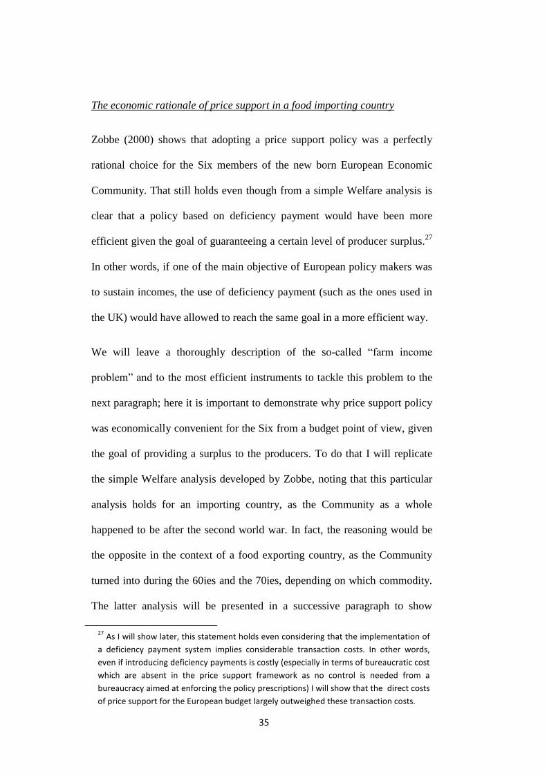
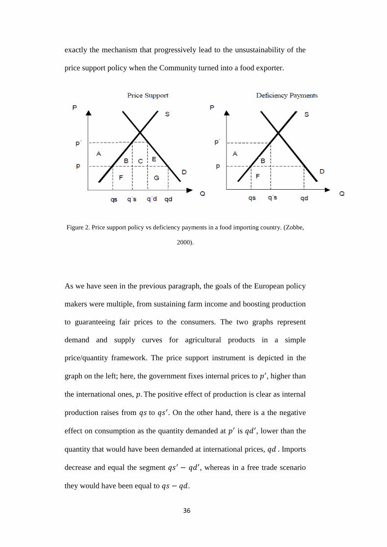
As we have seen in the previous paragraph, the goals of the European policy

makers were multiple, from sustaining farm income and boosting production

to guaranteeing fair prices to the consumers. The two graphs represent

demand and supply curves for agricultural products in a simple

price/quantity framework. The price support instrument is depicted in the

graph on the left; here, the government fixes internal prices to 𝑝′, higher than

the international ones, 𝑝. The positive effect of production is clear as internal

production raises from 𝑞𝑠 to 𝑞𝑠′. On the other hand, there is a the negative

effect on consumption as the quantity demanded at 𝑝′ is 𝑞𝑑′, lower than the

quantity that would have been demanded at international prices, 𝑞𝑑 . Imports

decrease and equal the segment 𝑞𝑠′ − 𝑞𝑑′, whereas in a free trade scenario

they would have been equal to 𝑞𝑠 − 𝑞𝑑.

37

Coming to the Welfare analysis, the policy triggers the following changes in

comparison to the free trade scenario. There is a producer gain equal to the

area A which is more than compensated by a consumer loss equal to the sum

of areas A, B, C and E.

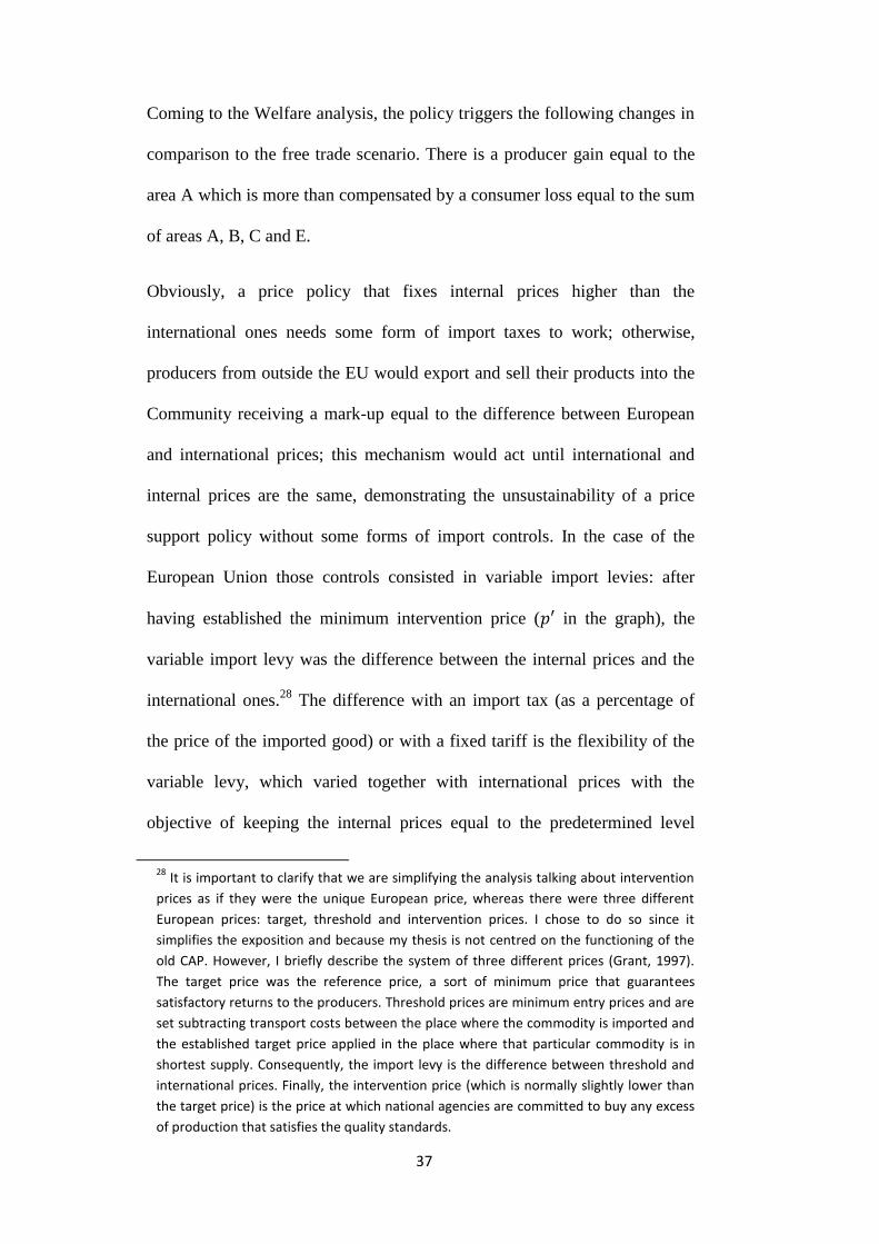
Obviously, a price policy that fixes internal prices higher than the

international ones needs some form of import taxes to work; otherwise,

producers from outside the EU would export and sell their products into the

Community receiving a mark-up equal to the difference between European

and international prices; this mechanism would act until international and

internal prices are the same, demonstrating the unsustainability of a price

support policy without some forms of import controls. In the case of the

European Union those controls consisted in variable import levies: after

having established the minimum intervention price (𝑝′ in the graph), the

variable import levy was the difference between the internal prices and the

international ones.28

The difference with an import tax (as a percentage of

the price of the imported good) or with a fixed tariff is the flexibility of the

variable levy, which varied together with international prices with the

objective of keeping the internal prices equal to the predetermined level

28

It is important to clarify that we are simplifying the analysis talking about intervention

prices as if they were the unique European price, whereas there were three different

European prices: target, threshold and intervention prices. I chose to do so since it

simplifies the exposition and because my thesis is not centred on the functioning of the

old CAP. However, I briefly describe the system of three different prices (Grant, 1997).

The target price was the reference price, a sort of minimum price that guarantees

satisfactory returns to the producers. Threshold prices are minimum entry prices and are

set subtracting transport costs between the place where the commodity is imported and

the established target price applied in the place where that particular commodity is in

shortest supply. Consequently, the import levy is the difference between threshold and

international prices. Finally, the intervention price (which is normally slightly lower than

the target price) is the price at which national agencies are committed to buy any excess

of production that satisfies the quality standards.

38

𝑝′. 29 The revenue from the variable import levy is the area C. Hence, the net

loss of the price support policy in comparison to a free trade scenario is the

sum of areas C and E.

The overall result is that consumers bear the costs of a policy that benefit

producers and, as long as the country is a food importer, the government. To

complete the analysis another positive side effect of the policy is the

reduction in imports, which allowed the government to “save” areas F and G

in terms of foreign currencies in a context where those currencies needed for

imports were scarce.

The Welfare analysis of the deficiency payments as an alternative tool to

reach the same goal of sustaining producers income is depicted on the right

of figure 2. As for the price support, producers are guaranteed an

intervention price that kept internal (producer) prices higher than

international ones, with the same producer gain of area A in comparison

with the non-intervention scenario. Internal production is boosted in the

same measure while consumers benefit from the lower international prices

and consumption increases to 𝑞𝑑 as it would be in the free trade scenario. In

fact, probably the biggest difference with the price support policy is that the

policy institutes two different prices, one (normally higher) for producers

and one for consumers (the international prices); hence the costs of the

policy are on taxpayers, who now have to finance direct transfers to farmers

via general taxation, and not on the consumers via higher (consumer) prices.

29

Another difference with a fixed import tariff or with a tax on imported products is that

when international prices were higher than the internal ones the system no longer

needed to operate and was automatically de-activated.

39

Imports are not taxed and increase to the segment 𝑞𝑑 – 𝑞𝑠′, the internal

consumer price is 𝑝 and it is the government that corresponds to the

producers the difference between international and internal prices through

deficiency payments (equal to the sum of area B and A). The net loss of the

policy in comparison with free trade scenario is B.

To sum up, from a purely efficiency perspective and without considering the

transaction costs implied by the deficiency payments to simplify the

analysis30

, deficiency payments should be theoretically preferred to price

support by a food importing country which aims at sustaining producers

income (the net overall gain over price support equals area E). However, it

should be now clear that from the budget’s perspective price support was the

better solution: the government actually gained from price support. The costs

of the policy were borne by consumers and government gained C taxing

imports with the variable levy equal to the difference between international

and internal prices,31

whereas in the deficiency payment scenario the budget

would run a deficit of B+A.

This positive effect on the communitarian budget was probably the main

reason that lead the Six to the adoption of the price support and it is not

surprising if we add to that the historical reasons seen in the previous

paragraph. Moreover, taking a closer look to some data regarding the trade

30

As specified in note 26, this omission can be justified on the basis that when I will

show the magnitude of the negative effects on the European budget due to the price

support, accounting for the transaction costs of direct payments will become a

secondary issue. To be clearer, if the comparison between the two system gave a

marginal preference of direct payments, then including transaction cost could change

our conclusions; however, since I believe that the economic benefit of direct payments

will largely outweigh its additional cost when the European countries started to be large

exporters, omitting this element from the analysis should not affect our conclusions. 31

Precisely between international and threshold prices. See note 26.

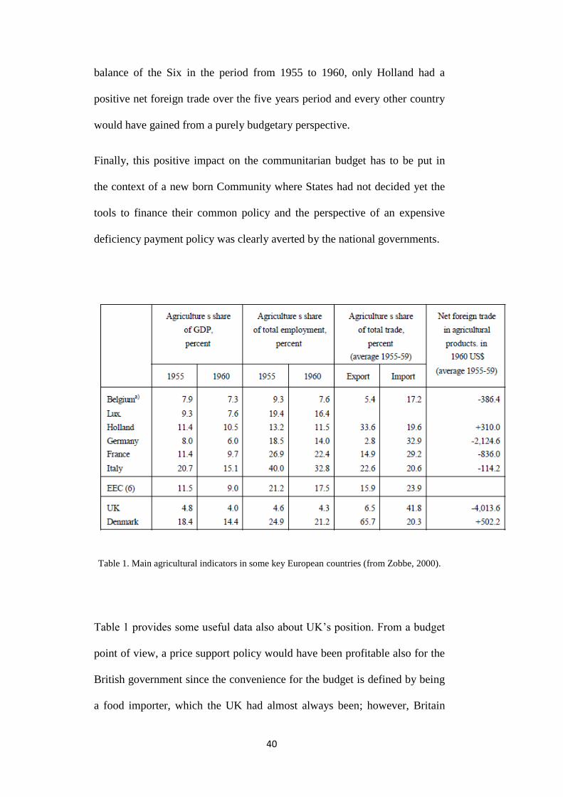
40

balance of the Six in the period from 1955 to 1960, only Holland had a

positive net foreign trade over the five years period and every other country

would have gained from a purely budgetary perspective.

Finally, this positive impact on the communitarian budget has to be put in

the context of a new born Community where States had not decided yet the

tools to finance their common policy and the perspective of an expensive

deficiency payment policy was clearly averted by the national governments.

Table 1. Main agricultural indicators in some key European countries (from Zobbe, 2000).

Table 1 provides some useful data also about UK’s position. From a budget

point of view, a price support policy would have been profitable also for the

British government since the convenience for the budget is defined by being

a food importer, which the UK had almost always been; however, Britain

41

chose deficiency payments and initially left the negotiations to be part of the

EEC. More than the result of a government aiming at maximizing overall

social Welfare, the reason of that choice probably lies in UK’s data of

agricultural share of total employment and in the bargaining powers of

British industrial and agricultural interests. Going back to O’ Rourke’s two

sector’s model, UK already largely experienced the internal migration from

countries to cities that follows trade liberalization, with the consequent

downward effect on nominal wages and a potential rise in unemployment

due to the difficulty to reallocate the excessive labour from agriculture to the

industrial sector. In other words the cost of living effect was bigger than the

labour demand effect and the overall effect on real wages would have been

positive. Moreover, the number of people in the farming sector was smaller

enough to run a deficiency payment scheme financed by government’s

budget, allowing UK to benefit from the overall welfare gains regardless the

positive transfers to producers.

The position of the Six was clearly different. In 1955 agriculture’s share of

total employment was lower than 10% only in Belgium, whereas in countries

such as France and Italy the figure was 26.9 and 40%. In this particular

context guaranteeing the same producer surplus through deficiency payment

would have been unsustainable for the European budget.32

On the other

hand, price support transferred that cost indirectly on consumers via higher

prices, which turned protection into a benefit for the government budget. On

32

In my opinion, the reluctance of the European countries to introduce deficiency payments from the very beginning has its main cause in the huge costs that this choice would have implied for the budget. In other words, they preferred to spread the costs on consumers via higher food prices and only in a second moment, when the number of people employed in agriculture was substantially smaller, they agreed on a direct payments system such as the one of the Mac Sharry reform.

42

the top of that, economic growth of the Six members in the 60ies eased the

acceptance of higher prices by consumers since the continuous increases in

nominal wages increased the purchase power of European consumers

regardless the high food prices.

To conclude, while UK had already dealt with the problems of the

industrialization process and had a strong interest to keep following a free

trade policy to boost its industrial sector, European countries were worried

that opening their markets to imports would have triggered a huge farm

exodus and potentially unemployment if not regulated; moreover, the option

to sustain farm income through more efficient instruments such as deficiency

payments was unsustainable for the budget whereas price support had the

benefit of being a source of revenue for the budget that could have been paid

indirectly via consumers in an context of economic growth.

Obviously, these considerations hold given the nature of the ECC as a food

importer. In Chapter 4, I will analyze the functioning of price support in a

food exporting country, which the Community soon became, and show how

the policy became progressively unsustainable for the same (budgetary)

reasons that were initially part of its strengths. Before moving to that, the

next chapter briefly describes the main arguments behind the idea of public

intervention in the farming sector focusing on what has been called the ‘farm

income’ problem in the literature.

43

1.3 The farm income problem: optimality of a price support policy to

support income

In the previous chapter I have shown the historical and economic reasons for

adopting a price support policy as a tool to sustain farm incomes and to

regulate the process of internal migration from the agricultural sector to the

developing industrial one. The underlying idea is that, in a free market, the

family based agricultural sector would have been displaced by cheap

imports. That feature might be thought to be specific of European agriculture

after the second world war and in some degree it is still today what

distinguishes it from the highly productive agricultural sector of the US and

other exporting countries, where mechanisation, dimension of holdings and

total factor productivity are higher than in Europe regardless the progresses

made by European agriculture in the past.33

However, the idea of a structural

weakness of the farming sector in comparison with other sectors of the

economy has pervaded agricultural economics literature from its beginning,

justifying practices of state intervention to regulate markets and sustain farm

income which systematically lagged behind non-agricultural income.

The objective of this paragraph is to provide a description of the so-called

farm problem since this is the argument that has been used to justify

transfers to producers. As we will see, there is not a unanimous position on

the fact that the farm problem is bound to characterize agriculture in any

44

possible scenario: some authors34

use recent data to assert that the problem

has been overcome by the developing of modern highly productive

agriculture and by an increase in the flexibility of the labour market, which

can now absorb rural exodus into the other sectors of the economy

guaranteeing the equivalence between agricultural and non-agricultural

income that is predicted by standard neoclassic theory.35

Besides this

potentially valid critique to the “farm income” argument, the main objective

here is not to provide a final answer regarding the farm income problem but

highlighting how this argument has been used to justify State intervention.

As regards this, the goal would rather be establishing whether price policy

was an effective policy to sustain incomes of marginal farmers; in other

words, assuming the validity of the “farm income” problem, was the use of

price support appropriate or the CEE should have used alternative

instruments to boost incomes of marginal farmers? I will proceed outlining

the literature on the farm problem, its critique and evolution. Then, I will

move to the actual goal of the chapter, commenting on the efficacy of price

support as an income support.

34

B. L. Gardner, (1992), “Changing economic perspective on the farm problem”, in “Journal

of Economic Literature”, Vol. XXX (March 1992), pp. 62-101 35

For example we have seen this predicted convergence between agricultural and non

agricultural incomes in O’Rourke’s (1997) contribution.

45

The farm income problem: short and long run factors

In his book, Ackrill (2000) makes a distinction between short run and long

run reasons that are normally used to consider the agricultural sector as

different from other sectors and justify some degrees of State intervention.

Among the first set, he stresses the short term variability of farm incomes as

a distinctive characteristic of the agricultural sector in comparison to any

other economic activity. In fact, agriculture is characterized by two unique

features: the relative stability (rigidity) of demand regardless price variation

due to the very nature of food as a necessity good and, more importantly, the

structural uncertainty about the level of aggregate supply, which depends on

conditions that are not controllable by the farmer and which might heavily

affect production (such as weather conditions and events that can drastically

change the final level of aggregate supply).

These two elements are clearly unique and limited to the agricultural sector.

In fact, for other types of goods (in practice for every good which is not a

necessity good and in some respects for luxury goods) the inelasticity of

demand does not hold and it responds quite well to price variations.

Moreover, in sectors that do not depend so much on external conditions for

the production process there is normally the possibility to predict quite

accurately the final level of supply given the amount of inputs used: in other

words, supply is easily predictable and can vary to match demand.

What causes instability of agricultural incomes in the short run is the

combination of these two characteristic: while demand is fairly stable (very

46

rigid) at any price, the fluctuations in supply result in very large price (and

possibly income) variation.36

This variability in farmers income, depending

on factors the farmers cannot control, partially justifies market intervention

to stabilize prices at least in the short run. This justification is even amplified

by the fact that one of the result of income variability has normally been a

more conservative attitude, by the farmers, regarding investment and

production decisions in general.

As regards the long run reasons for State intervention, the argument is about

structurally declining commodity prices and income. If in the short term

problems are limited to an uncertainty of farm prices and incomes, the

traditional literature on the farm problem has highlighted that in the long run

the real problem is that prices and incomes are bound to decline due to a

mechanism known as the “treadmill” (Cochrane, 1958)37

. Moreover, the fall

in incomes is both in absolute and in relative terms (compared with non-

agricultural incomes) giving quite a strong reason for State intervention to

counteract this mechanism with some form of subsidy.

36

It would be fairly easy to provide a simple graph analysis that shows how a more rigid

demand leads to more pronounced price variations, given the same shock in the level of

aggregate supply. More difficult is to prove the consequent effect on incomes because

even if it is true that prices are declining, there is still the possibility that the producer

increases production in an amount that outweighs the price decrease, with an overall

positive effect on income. However, in the short run the possibility to compensate the

price decrease with an increase in supply is unlikely so we have this short term

uncertainty of incomes as a result of price fluctuations. This reasoning about technical

progress and increase in production as a way to avert income fall is crucial to explain the

long drivers of incomes decrease: on one hand, only innovators who significantly increase

their production manage to keep (or increase) their incomes. However, on the other

hand the aggregate effect of a myriad of innovators is that the excess of supply is even

greater and hence the price decrease and the downward effect on incomes, in a vicious

cycle as the one described by Cochrane in his “treadmill theory”. 37

Cochrane, Willard W. “Farm prices, myth and reality”. Minneapolis: U. of Minnesota Press, 1958.

47

The absolute fall in income would result from the tendency of supply to rise

over time driven by technical progress, whereas demand is static: this

automatically leads to downward pressure on prices and to a decrease in

absolute incomes, especially for smaller farmers which cannot compensate

the price decrease by a substantial increase in output.

The decline in relative incomes compared to other sectors of the economy,

instead, is due to the “Engle-effect” which says that food’s share of total

expense declines with increasing incomes. This happens for several reasons,

the first of which is that with raising incomes people start consuming more

non-necessity goods and therefore, even if the absolute expense in food

increases, the relative share of food out of total expense decreases. Also, as

income rises, it is likely that a growing percentage of the total expense on

food goes to the marketing and other non-food margins.

To sum up, not only the absolute level of farm income but, most of all, the

relative farm income is bound to decrease in comparison with other sectors

as the share of total spending going on farm output falls.

Gardner (1992) provides an extensive review of the literature on the farm

problem and especially about the main critiques to the argument; he stresses

that the definition of the farm problem is an issue which includes both the

problem of the excessive variability and the relative lower level of

agricultural in comparison with non-agricultural incomes.. As stated above I

will briefly summarize the development of the “treadmill theory” and its

limitations without the aim of providing a final answer on the farm problem.

My goal is rather to use some basics microeconomic analysis to comment on

48

the efficiency of a price support policy to sustain incomes assuming the

validity of the farm income problem and hence the justification of State

intervention in agriculture. In other words, more than validating or not the

farm income problem I will try to show that an indiscriminate price support

was not the most efficient instrument to sustain marginal farms’ income and

that the policy ended up favouring large farms.

The first formulation of the farm problem comes from the work of Schulze

(1945)38

, who defined the double aspect of the farm problem in its short and

long term nature and justified State intervention to remedy to the long term

downward pressure on incomes.39

Cochrane (1958) formalized the model in

a more rigorous partial equilibrium framework adding technical progress:

the central assumption is again that in the long run supply grows at a faster

rate than demand, provoking a downward pressure on prices. The

mechanism turns into a vicious cycle including technical progress. In fact,

technical progress can be considered the driving factor of the “treadmill

theory” and explains the structural tendency of declining commodity prices.

The mechanism is the following: in a context of declining prices (and

pressures on incomes) some farmers invest in technical progress to lower

production costs and produce more. These farmers have benefits, at least in

the short run, since also with declining prices they can now produce and sell

more thanks to lower production costs. The effect on the farmers that do not

innovate exacerbates the downward pressure on income as the increase in

38

Schults, T. W. Agriculture in an unstable economy. NY: McCraw Hill, 1945. 39

Schultz provides estimate of agricultural and non agricultural incomes, in the US, for

the period between the 1930 to the II world war and concludes farm incomes were equal

to a merely 30/40% of the non agricultural incomes.

49

production by the innovators is likely to reinforce the overall price reduction.

Therefore, everyone must innovate to minimize losses lowering production

costs and maximizing production. The overall effect is a substantial increase

in production that lowers the prices even more, in a vicious cycle where first

innovators succeed temporarily to safeguard their incomes, but the overall

effect of their investment is an even more pronounced decline in prices (and

therefore, most probably, in incomes).

It is obviously possible that some (big) producers succeed in increasing

production more than the amount of price decrease, with a consequent raise

in their income. However, the standard effect is that the increase in

production that follows technical progress is outweighed by the price

reduction, with an overall negative effect on incomes: this is, in a nutshell,

Cochrane’s (1958) treadmill theory, a partial equilibrium model that explains

low farm income as the aggregate result of the forces described above.

One of the first critiques to the treadmill theory and especially regarding the

prediction of a persistent income gap between agricultural and non-

agricultural incomes came with the development of general equilibrium

models that insert the agricultural sector into the overall economy,

overcoming the limitations of partial equilibrium analysis. With the aim of

completing the analysis including links between sectors in the model, they

often used the assumption of perfect labour mobility to include the

possibility that the excess labour in agriculture could move to other sectors,

harmonising wages and more generally incomes between sectors. In fact,

with perfect labour mobility we should not experience relative lower wage in

agriculture as the excess of labour would leave the sector readjusting

50

nominal wages between agricultural and non-agricultural sector: even if the

“treadmill” is still in place resulting in decreasing food prices, labour would

leave the sector re-harmonising nominal wages.

O’Rourke’s simple two-sectors model is a good example of the results

obtained including other sectors in the model, predicting that the rural

exodus would lead to a decrease in wages in both agricultural and non-

agricultural sectors as the readjustment would continue until wages are

harmonised. However, as Houthakker (1967)40

underlies, if the increase in

technical progress and the downward effect on prices is substantial and the

outflow of labour is not fast enough, there could be a discrepancy between

the two wages. That would mean that the adjustment process is not complete

and that there is an excess of labour in the agricultural sector. Johnson

(1959)41

put it simply: “the farm problem is the result of the employment in

agriculture that can earn as large a real income as the same labour could earn

elsewhere in the economy”.

The question then is: why the readjustment is not complete? Why does

labour stay in a sector even if unable to earn an income as large as the one

achievable outside agriculture? Why the prediction of income harmonisation

between sectors does not seem to hold, at least for some historical cases and

periods?

In other words, if the treadmill theory explains the structural downward

trend of commodity prices, in order to explain why also incomes are bound

40

H. Houthakker. "Economic Policy for the Farm Sector." American Enterprise Institute,

Washington, DC, 1967. 41

D. Gale Johnson, "The Dimensions of the Farm Problem," in Problems and policies of

American agriculture. Ed.: EARL O. HEADY. Ames: Iowa State U. Press, 1959, pp. 47-62.

51

to decrease we have to rely on some other theory that explains why labour is

not perfectly mobile between sectors, resulting in over-employment in

agriculture and lower incomes in comparison to the other sectors of the

economy. Answering this question is even more compelling since data

clearly show that the income gap is persistent, or at least has been for some

considerable periods.42

As Gardner summarizes, the explanations provided by the theory

incorporates thesis like different types of technical progress between sectors,

with the one that affects agriculture that would be mainly labour saving and

others that try to explain the gap with objective and measurable differences

in skills, age and sex between agricultural and non-agricultural workers

(Johnson, 1953)43

. This kind of neoclassical explanation, in fact, consider the

farm income problem mainly as a short run phenomenon due to the presence

of some adjustment costs in labour reallocation between sectors and uses the

aforementioned differences in skills and other variables as a (weak)

explanation of long term effects.

However, probably the most convincing theory to explain persistence of

income gaps comes from the asset fixity theory (Johnson, 195844

; Hathway,

42

Benedict, “Farm policies of the United States: 1790-1950”, New York: The Twentieth

Century Fund, 1953, adds further evidence to Schulze’s estimate of the income gap. He

infers that agricultural incomes as remained between 40% and 60% of non agricultural

incomes respectively in 1930s and in the years that followed the II world war. As regards

the current situation, Gardner (1992) seems to defend the idea that recently also the

empirical evidence would be less supportive of the ‘farm income’ thesis. 43

J. Gale Johnson, "Comparability of Labor Capacities of Farm and Nonfarm Labor,"

American Economic Review, June 1953, 43(3), pp. 296-313. 44

J. Gale Johnson, " An Appraisal of the Data for Farm Families," in An appraisal of the

1950 census income data. NBER studies in Income and Wealth, Vol. 23, Princeton:

Princeton U. Press, 1958a, pp. 287- 301.

52

196445

and Quance, 197246

). The claim is that when an investment in an

asset has to be made (for example the purchase of a tractor or of additional

land) the farmer compares the returns of this investment to the returns he

might expect to have investing in some other sector and therefore exiting

agriculture. The fact is that since many farmers make the same investment

decisions the actual returns of their investment might well be lower than the

estimates that lead them to carry out the purchase in the first place. Some of

them would probably like to withdraw the investment but that might be

difficult as the majority of these factors are sector specific. Also they would

be worthy less than when the farmer bought them, again as a result of the

aggregate overinvestment. The farmer is then committed to its investment

since he cannot use directly the factor he bought in another sector and

because he probably would not accept to bear the loss of selling the asset at a

(lower) price than the purchase one. We should now explain why farmers

took their investment decisions in the first place since we have seen that

there is a structural and constant tendency of price decreases and the answer

of the asset fixity theory is that temporary increases in prices can lead

farmers to overestimate the returns of the investment; in fact, when most of

them take the same decision, the aggregate overinvestment boosts supply

and, with rigid demand, decreases prices, leaving the farmers with assets that

are not as profitable as they thought, are sector specific and cannot be sold if

not at a consistent loss.

45

Hathaway, D. E. (1964) “Problems of progress in the agricultural economy”. Glenview,

IL: Scott, Foresman,. 46

Quance, L. (1972) “The overproduction trap in U. S. Agriculture”. Baltimore: Johns

Hopkins U. Press, 1972.

53

Now that I have analysed in more depth the nature of the farm income

problem and its explanation of why also in the long run there could be a gap

between agricultural and not agricultural incomes I will move to the main

goal of this chapter, which is to verify whether price support is an efficient

response to the declining agricultural incomes.47

In other words, given the

reality of a farm problem affecting the European countries after the second

world war, I will try to show if price support was in practice the better tool

to counteract this phenomenon.

47

As declared at the very beginning, I do not try to verify whether data confirm the

predictions of this theory (even if some evidence from other studies has been

referenced). In fact, since the farm problem has been used to justify State intervention to

sustain farm incomes, that would not be so relevant as anyway the State intervention has

occurred. It is instead way more important to check whether price support has been an

efficient tool to reach the stated goal of sustaining farm incomes.

54

Is price support the optimal response to solve farm income problem?

Regarding the Welfare effect of price support, the common claim is that this

instrument favoured large producers instead of the small family farms whose

incomes were the ones that actually needed to be sustained (Lanfranchi,

2008; Commission Green paper, 198548

). Hence a first limit of price support

can be found in its uneven distributional effects.

The Green paper of 1985 has analysed the distributional effects of price

policy, evaluating its efficacy in achieving the multiple set of goals of the

CAP. Written in a context where the Community already became a food

exporter and was facing the problem of agricultural surpluses, the report

states that price policy has been effective in boosting technical progress and

increasing production. The problem of the surpluses itself was the prove of

the efficacy of price support in enhancing agricultural productivity.49

However, regarding the distributional effects, the Green paper highlighted

the failure of the instrument to adequately sustain incomes of marginal

farmers. Considering the economic environment and the high rates of

unemployment that Europe experienced in the seventies, after the economic

boom post II world war, sustaining marginal incomes and therefore

managing the farm exodus was an important goal of the CAP. In that

48

European Commission, 1985. “Perspectives for the common agricultural policy. Communication of the Commission to the Council and the Parliament”. 49

For a more detailed analysis of the links between price support and productivity please

refer to chapter 1.5 and in particular to the studies of Perin and Fulginiti (1993)

Kalaitzandonakes (1994), Van deer Mer and Yamada (1990). Oskam and Stefanou, in

Harvey (1997) provide a summary of the literature on the links between price support

and technical change.

55

respect, the paper highlights how a type of support based on the guarantee of

a minimum price was scarcely effective in targeting the segment of

producers that were really in need of economic help: what happened is that

price support was still relatively too low to be effective in sustaining income

of marginal farmers, whereas was big enough to create an incentive for

bigger producers to invest in technical progress and, consequently, increase

production substantially.

To have an idea of the disproportion between funds received by different

types of producers, another report of the European Commission (EC, 1994)50

provides an estimate of the subdivision of European money between

commercial and family farms, calculating that approximately 80% of total

CAP spending was going to the 20% bigger farms, whereas the remaining

80% of small sized family farms received just 20% of CAP spending.

Understanding why a mechanism like price support ended up favouring large

farms is quite straightforward and Kean and Lucey (1997)51

provide an

exhaustive list of the factors that determine this disproportion. I will quickly

outline four factors and I will dedicate more space to the reason that I

believe is predominant among the others, helping the explanation with a

simple graph analysis developed by Baldwin (2002).

The two authors52

identify the following five reasons for the disproportion in

European support between large and small producers. First of all they claim

50

European Commission (1994) “EC Agricultural Policy for the 21st Century”. 51

Kean and Lucey (1997) “The CAP and the Farmer” in Harvey, “The Common Agricultural

Policy”, 1997. 52

For further details have a look at “Farm Employment and Economic adjustment in

OECD countries”, OECD, Paris (1994).

56

that support policies have normally regarded commodities produced by large

farms, for example cereals and diary and milk products. This assertion is

self-evident and the fact that commodities like most of vegetables and fruits,

normally produced by small scale business, received virtually no support

from the Commission explains part of the protests of small farmers towards

a policy that has instead financed large landowners.53

Another reason is that since supply is normally more elastic for big

producers they normally can increase production more easily in response to

publicly provided incentives as higher commodity prices. The fact that large

producers have an higher elasticity of supply is fairly intuitive as they

probably have resources (in terms of funds to increase input use) ready to

use to maximize production. The reasoning is that, assured they will enjoy

high prices by the Commission, large producers actually maximize the

benefits increasing production substantially whereas small family business

could be income constrained and unable to increase production by the same

proportion.

A third reason, similar to the one just mentioned, is that large farms have

normally more funds to expand their dimension buying or renting new land

in response to price increases whereas small producers are more inelastic.

53

Regarding this is widely known the controversy regarding the fact that very big

landowners such as the English Royal family have historically received a huge amount of

support from the CAP. The debate has continued after Mac Sharry and Fischler reforms

because, as we will see in due time, also with the new system based on direct payments

the criteria used to calculate direct payments have not been to target smaller and poorer

producers (even if with the new instrument it would have been easier to target a specific

group of producers).

57

The fourth reason is related to the fact that types of subsidies such as price

support tend to be incorporated into land values; as it will be analysed later

talking about direct payments, almost every type of direct or indirect subsidy

tends to be subject of this limit. As regards price support, the mechanism is

that the higher price paid for cereals tended to be captured into land prices

with the result that the real beneficiaries of such policy were predominantly

large land owners. If we think about small and large owners, in fact, it is

straightforward that, even if the benefit in terms of value of their asset was

proportional (depending on how intervention price was higher than

international prices a certain hectare would have had an increase in value

both for small and large producers), large owners saw the value of their asset

increase substantially more in absolute value; if we consider that together

with the third reason mentioned above, it is easy to see how this “rent effect”

tends to be greater and favour larger farmers. Moreover, another aspect of

this tendency of subsidies to end up in rents is that the actual farmer might

not be anymore the real beneficiary of the price support. Thinking about a

situation where a small farmer rents land from a landowner that has exited

the sector, the person that would benefit from price support would not be the

farmer but the unproductive landowner, besides how the subsidy is allocated

legally (in fact, even is assigned to the farmer the landowner would probably

be able to extract an additional rent and “capture” the value of the subsidy).

Given that the goal of the policy was to support agricultural incomes, this

fact is itself a symptom of the misconception of the policy and the negative

effects could be even worse if the renting part is a small farmer that does that

to increase his revenues.

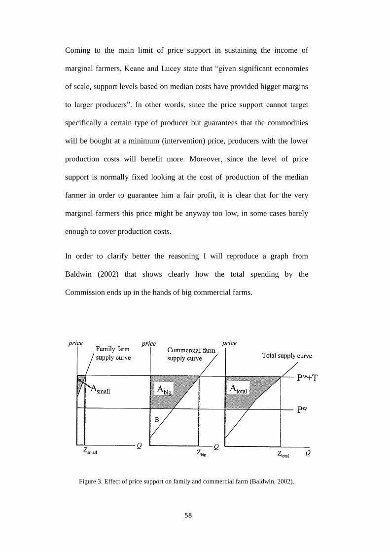
58

Coming to the main limit of price support in sustaining the income of

marginal farmers, Keane and Lucey state that “given significant economies

of scale, support levels based on median costs have provided bigger margins

to larger producers”. In other words, since the price support cannot target

specifically a certain type of producer but guarantees that the commodities

will be bought at a minimum (intervention) price, producers with the lower

production costs will benefit more. Moreover, since the level of price

support is normally fixed looking at the cost of production of the median

farmer in order to guarantee him a fair profit, it is clear that for the very

marginal farmers this price might be anyway too low, in some cases barely

enough to cover production costs.

In order to clarify better the reasoning I will reproduce a graph from

Baldwin (2002) that shows clearly how the total spending by the

Commission ends up in the hands of big commercial farms.

Figure 3. Effect of price support on family and commercial farm (Baldwin, 2002).

59

The graph replicates quite clearly the situation of European agriculture for

the period considered. It shows how the concerns of policy makers and farm

organisations were probably justified since a large number of family farms

would have been expelled from the market if international prices were to be

applied. It also suggests that price support helped slowing down the rural

exodus making production viable for a large part of marginal farmers.54

In fact, in the graph Baldwin depicts the situation where without intervention

from the Commission, just the big commercial firms would have marginal

costs that would be low enough to make production profitable also at

international prices. For simplicity we assume that all marginal farmers

would exit production, whereas with price intervention also the small family

farms would be able to make a profit. Anyway, the interesting feature of this

graph is in the quadrant on the right, where the aggregate supply curve is

constructed as the horizontal sum of individual supply curves. The area 𝐴𝑡𝑜𝑡

represents the total amount of money paid by intervention agencies to fill the

difference between international and intervention prices. As we can see it is

divided between 𝐴𝑏𝑖𝑔 and 𝐴𝑠𝑚𝑎𝑙𝑙 and it is clear that the vast majority of the

expense goes to bigger farms, providing an intuitive graph explanation of the

data provided by the Commission on the disproportion between small and

big farms.

54

Obviously, rural exodus and farm adjustment in terms of expansion and modernization

of the holdings occorre anyway, as it is clear by data regarding the number of people

employed ion agriculture (see, for instance, Keane and Lucy Table 1 in their contribution

in Harvey, 1997). The point here is that without some kind of support the exodus would

have been too fast with consequent problems in terms of unemployment (and possibly

environmental losses), as thoroughly discussed in the chapters before.

60

At this point is possible to draw a final judgment on the role of price support

in the so-called “old CAP”. It can be concluded that it was first chosen for

historical and budgetary reasons, at least until the Community remained a

food importer. Regarding the reason behind the very existence of State

intervention I have outlined the literature on the farm problem even though a

detailed analysis on its enduring validity is omitted. I used, instead, that

argument to see whether a specific intervention tool such as price support

has been effective in sustaining the incomes of marginal farmers and the

answer has been at least partially negative since the bigger recipients of

European agricultural expense were large commercial farms. In fact, the use

of direct payments would have been preferable, specifically because they

could have been used to target a specific segment of farmers depending on

their level of income, hence avoiding to favour production units already

highly competitive at market prices. However, it is important to note that at

the very beginning price support was a policy that created revenue for the

European budget and this crude fact might explain why the use of (more or

less) targeted direct payments was left aside. Price support allowed the

Community to spread the cost of the policy on consumers via high food

prices and that was somewhat acceptable in a situation of economic growth

and improving standard of living. Direct payments, instead, should have

been financed by the taxpayer, and therefore they were very expensive for

the European budget, especially in a situation where the number of farmers

that would have been eligible for the payments was still representing, for

some countries, the relative majority of the working population. This type of

support would have become more and more economically viable as soon as

61

the number of people employed in agriculture shrank, meaning a decreased

pressure on the European budget.

In the first chapter of the second part I will go back to the topic of which

support would be optimal to achieve the multiple set of goals that

characterized the CAP, showing that some of the proposals of reform were

based on the idea that only using structural policy (maybe together with

some forms of targeted direct payments) it would be possible to solve the

problem of marginal farmers at its roots.55

55

In particular, the Commission’s report under Commissioner Mansholt (1968) and Mansholt’s speech were the first documents where the Community realized the problems associated with price support, namely the incentive to overproduce to maximize profits and the perverse distributional effects of such an instrument.

62

1.4 The functioning of a price support policy in a food exporting

country

In chapter 1.2 I have shown the historical and economic reasons for the

adoption of price support as the central instrument of the “old CAP”,

whereas in the last chapter the classic justification of State intervention has

been outlined, together with the limitations of price support in safeguarding

incomes of marginal farmers.

In this chapter I will go back to the history of the CAP outlined in chapter

1.1, describing the Community shift from being a food importer to a food

exporter. The consequences for the European budget are clear and will be

analysed quickly, together with a quick mention of the literature about the

links between price support and farm productivity. Most importantly, I will

also describe how the very mechanism of price fixing and the “green

money” system concurred in worsening the pressures on the European

budget, demonstrating that the ‘old CAP’ had to be reformed to avoid a

vicious cycle that have led to its total unsustainability from a pure budgetary

perspective. I will proceed with a detailed analysis of the latter points since it

is a precondition to understand why the Community quickly became a food

exporter and soon suffered from a high budget deficit to sustain the CAP.

63

Price fixing and the effect of the Luxemburg compromise

In chapter 1.1 the historical reconstruction terminated with the decisions

took in the early months of 1962, which constitute the official birth of the

CAP (Fearne, 1997) based on the principles of market unity, financial

solidarity and Community preference. However, a number of fundamental

issues were still to be agreed in order to make the policy effectively

operating, first of all an agreement on the level of common prices. As

regards this matter, the conflict was between countries with relatively low

and high production costs, which claimed for, respectively lower and higher

levels of price support.

Germany in particular embraced the position of guaranteeing high

intervention prices for cereals to defend its highly inefficient farm sector.

For other countries (such as France) with relatively lower production costs,

high prices meant that probably production would have exceeded demand,

with the consequence that export restitution became necessary (or crop

destruction) to avoid the extra production to be sold on the national (or

European) market with the effect of lowering the same intervention prices

that were agreed by the Commission. Obviously these export restitution had

a cost and, in a situation where the financing of the CAP budget still had to

be agreed, countries like France feared that the burden of the export

restitution might fall almost entirely on the national budgets, determining a

more careful position of price fixing. That was the content of the bargaining

in the years between 1962 and 1964.

64

Ackrill (2000)56

clearly explains that the solution of the issues regarding

price fixing and the financing of the policy were strictly correlated.

Regarding the negotiations of price levels, France threatened to withdraw

from the Community if the Germans still refused to accept a reduction in the

intervention price for cereals.57

In the last months of 1964 an agreement was

reached thanks to the decision of the German Minister of economic affairs58

to agree price reductions between 11 and 13% in comparison to the pre-CAP

levels.

Coming to the issue regarding policy financing we have seen that France,

who would have likely become a food exporter with too high prices, was

particularly concerned about reaching an agreement on how to finance the

policy before “own resources” would guarantee the autonomous functioning

of the Community.59

The Commission proposal of 1965 was strongly

opposed by the French not only because it increased substantially the level

of French contribution to the European budget, but especially because it

granted to the European Parliament the power to directly manage the

revenues of import levies. In other words France wanted to reach an

56

Ackrill (2000), op. Cit. Pag 35. 57

For further details, Neville-Rolfe, 1984, “The Politics of Agriculture in the European

Community”, London, Policy Studies Institute. 58

Kurt Schmücker, Federal Minister of Economics. October 17, 1963 – November 30,

1966. 59

Up until 1970 the only two sources of revenue of the Euroean Community were the

eventual revenues from the import levy of the CAP (as long as the Community remained

a food importer overall) and a series of national contributions to the European budget.

However, revenues from import levies were still managed by national governments (even

if a large part of them was to be given to the Community) and this was part of the French

opposition to the Commission proposal of 1965. In 1970 it was introduced an automatic

contribution based on a percentage of the national revenue coming from indirect

taxation (IVA in Italy) whereas in 1987 it was instituted also a contribution based on a

percentage on the Gross National Product of the members.

65

agreement on common financing since it was clear that with high prices it

would have experienced the need of conspicuous export restitution;

moreover, De Gaulle was trying to limit French national contributions

during the transitory period and to avoid any surrender of sovereignty

directly to the European Parliament. After six months during which the

French Foreign Minister deserted the Council of Minister Meetings an

agreement was reached at the Council of Luxembourg in January 1966. The

amount of countries contribution were agreed until 1970 but probably the

most important decision taken was that in the future every decision that

involved financial aspects (“whenever national interests are at stake”) should

have been taken by unanimous agreement and not by majority voting.

I have spent some time describing these decisions about common prices and

the rules of voting in the Council because, as it will be clear immediately,

they had a huge impact on the issue I analyse in this chapter: how the

Community became a food exporter and how price support turned into a

liability for the European budget.

Hubbard (1997)60

explains that since the price for cereal was fixed at a

disproportionately high level it triggered a sort of chain reaction regarding

the determination of the prices of the other commodities. Clearly,

guaranteeing high extra-remuneration for a certain commodity while keeping

intervention prices for the others at a relatively low level was not a viable

option because that would have deeply influenced production decisions in

favour of cereals, with the risk of massive overproduction and

60

L. Hubbard and J. Lingard “The CAP and the Developing world”, 1997, in Harvey, op. cit.

66

underproduction of the other, less subsidised commodities.61

Hence the

tendency to fix intervention prices well above international prices for a long

list of commodities and the extension of some kind of State intervention also

to products that were not safeguarded by national authorities before the

CAP.

Coming to the consequences of the Luxemburg compromise, it is quite clear

that after that precedent, every time new prices had to be fixed each State

could have claimed that the decision involved “vital national interests” and

that unanimity was necessary. The (predictable) result is that each country

tried to defend their specific products with a bargaining that was more likely

to reach an equilibrium on high rather than on low prices. Moreover, after

1970 the financing of the CAP with “European” resources and the final

abolition of internal barriers to trade also countries such as the Netherlands

that initially opposed high prices slightly changed their position. The reason

is that contrary to a situation where eventual surpluses had to be financed by

national budgets and where high prices would have affected considerably the

competitiveness of the products of the exporting countries, the possibility to

export on the European market at those high prices turned into an

opportunity for some producers, especially considering that for the

61

I would like to anticipate here that, anyway, the policy favored cereal productions in

general and in particular wheat. In fact, when the empirical test on the efficacy of

decoupling will be carried out in the second part it will appear that there has been a shift

away from cereal production. Therefore, if Mac Sharry’s reform triggered a reduction in

production levels due to the change of the support mechanism from price support to

direct payments, Fischler reform triggered a further reduction in cereal production due to

the fact that those payments were still partially coupled with the type of production,

reflecting the historical community preference for cereals (and, in particular, for wheat).

67

remaining produce it was now the European budget that would have born the

cost of export restitution.

To sum up, we can conclude that the first decision on high cereal prices and

the Luxemburg compromise determined a tendency to even higher prices

with the effect of worsening even more the problem of surpluses, as it will

be clear by the graph analysis that follows. Before that, I will describe also a

third element that concurred to this onward pressure on intervention price,

namely the so-called green money system that followed the crisis and the

collapse of the gold standard and characterised the CAP until the system

based on flexible exchange rates62

was replaced, the 1st of January of 1999

by a system of fixed exchange rates in preparation of the Euro.

62

In 1972 European countries negotiated the start of the so-called “Snake in the tunnel”,

a system that linked together the six European currencies allowing some band of

oscillations. This system was replaced in 1979 with the better structured European

Monetary System (EMS), which had anyway the same rationale behind its structure:

fixing exchange rates at a certain level but allowing currencies to float within limits.

68

The “green money system” and its consequences on price setting.

As Ritson and Swinbank (1997)63

highlight, the “green money system” has

been one of the most omitted aspects of the Common Agricultural Policy

because of its complexity, which often made it difficult to understand also

for the very policy makers involved in CAP negotiations at the European

level. The reason to open a parenthesis on this topic is to show how it

contributed to the upward effects on prices that eventually lead to the simple

unsustainability of the old CAP based on price support.

Starting with the historical reconstruction, after the common decision on the

level of prices for some main commodities, the principle of market unity

came under treat due to the end, in 1971, of the system based on fixed

exchange rates with respect to the dollar known as the system if Bretton

Woods. The start of the crisis was already evident in 1969, when global

economic turmoil put under pressure the very idea of fixed exchange rates.

In Europe, the German Marc was revaluated against the dollar while the

French franc devalued; the final end of the system occurred in 1971 and

European countries negotiated in 1972 a flexible exchange system that

allowed currencies to float (within limits) freely depending on market

conditions.

In order to provide a straightforward explanation of how the end of fixed

exchange rate triggered the aforementioned upward effect on prices, it has to

be noted that European Commodity prices were fixed in a common unit of

63

C. Ritson and A. Swinbank, “Europe’s Green Money”, In Harvey, 1997.

69

account, a fictional common currency (that has been the ECU since 1979)

and that before was a pure fictional currency calculated as a weighted

average of the currencies of the member States.

The question is: what happened when some countries re-valued or devalued

with respect to the reference currency? A practical example will help

clarifying the matter. Let’s use the Dollar as a reference currency to avoid

the complication that the ECU itself was a composition of the currencies of

the members of the European Community.

Assume that the wheat common price is fixed to 100 $ and that the

“agricultural conversion rate” is 0.5 for the Marc and 10 for the Lira. A ton

of wheat will cost 50 Marc in Germany and 1000 Lire in Italy, satisfying the

principle of common prices, which will be 100$ in both countries using the

same unit of account.

Let’s now analyse the situation of a currency revaluation or devaluation

starting from the case of a currency revaluation, as it happened for the Marc

in 1969.64

First of all we have to specify that the Commission made clear that it would

have not allowed the agricultural conversion rate to fluctuate together with

the flexible exchange rate as one of the objectives of the policy was to

64

The opposite case, currency devaluation, is not analyzed here as it is solved in an easier

way readjusting (increasing) the agricultural conversion rate for the country that

experienced a devaluation. Moreover, that does not lead to the same indirect upward

pressure on common prices as the actual increase in (nominal) prices happens just in the

devaluating country and it is overdue to avoid an actual decrease in real prices. The case is

therefore different from the one of revaluating country where to keep nominal prices

constant in the revaluating country (in effect increasing real prices) the readjustment

actually lead to a nominal (and real) price increase in all the other European partners.

70

guarantee price stability. Hence, the agricultural conversion rate was not

automatically adjusted to the fluctuations of the exchange rates, creating a

discrepancy between “green money” and the actual market value of different

currencies on the market.. Going back to the Marc revaluation, assume that

the exchange rate between Marc and Lira is 1 DM = 20 L so that the

following identity held before Marc revaluation 1DM = 2 $= 20 L.65

Now,

suppose that the Marc appreciates so that the following equality holds 1DM

= 2.5 $ = 25 L.

If the Community wanted to keep the common price of one ton of wheat

equal to 100 $ they should revise the agricultural conversion rate of the Marc

to 0.4 and paid just 40 Marc a ton of wheat to the German farmer. The

important thing to note is that in this case of currency appreciation, to keep

prices stable the Community should impose a (nominal) price decrease in the

country with the strong currency through a reduction of the agricultural

conversion rate (even if real prices would be still the same as the purchase

power of 40 Marc is now equivalent to 1000 Lire and equal to the common

unit of account, 100 $). The problem is that it was almost impossible to

impose such a revaluation of the agricultural conversion rates to the “strong

country” as that would imply a nominal price reduction totally opposed by

farm organisations. In fact, it was normally the case that the appreciating

country managed to keep its price to the original amount, 50 Marc.

This is exactly the moment were common pricing ends. What is happening is

that 1 ton of wheat is not worthy the same amount of money in the European

65

Remember that the Dollar is used here for simplicity as a substitute of the European

71

countries as it is worthy 50 Marc in Germany and 1000 Lira in Italy in a

situation where 50 Marc are equal to 1200 Lira on the currencies market.

The logical consequence is that Italian producers would have the incentive to

export their product in Germany, get 50 Marc for a ton and then convert

them into Lira to get an extra 200 Lira in comparison to the intervention

price they would be paid if selling on the national market. Not only, the

incentive would be even more perverse since Italian importers would import

food from outside the community paying it 1000 L per ton and then selling it

to Germany for the extra profit. This mechanism would then continue until

wheat price in Germany is equal to the international market (this result is

due to the no arbitrage condition),66

in a perverse mechanism where the

higher price paid in Germany indirectly triggers an increase in the

international prices of wheat at the expense of the European taxpayer (or

consumer, depending if the Community as a whole is a food importing or a

food exporting country and, hence, has a trade balance in active or passive).

66

In brief, the “no arbitrage condition” tells that the rule of one price will hold for different

markets if trade is free between them. In this case, the condition helps predict what would

have happened if prices were fixed at 50 Marc in Germany and 1000 Lira in Italy in a

situation where the exchange rates were actually 50 Marc = 1200 Lira. Italy would have

exported its products into Germany to get the equivalent of 1200 Lira. Not only, since free

trade was established between Italy and Germany, Italy would have imported food from

the rest of the world up until the situation where international prices equaled 1200 Lira

minus the value of the import levy between the Community and the rest of the world

unless the variable import levy was revised even upwards.

The main learning is that it was not possible to have different prices between countries if

free trade was established between them. In fact, MCAs where soon imposed between

European countries vanishing the principle of common market. In order to remove them

avoiding the aforementioned problem an increase of the agricultural conversion rate for

the weaker countries was necessary (together with an increase of the variable import levies

towards extra EU countries). Hence, the upwards pressures on prices and the worsening of

the external relations with the main trading partners.

72

The initial remedy adopted by the Community was to impose internal

Monetary Compensatory Amounts (MCAs), in this case an import levy of

200 Lire for any export of wheat from Italy and the other countries with

weaker currency into Germany. However, it is clear that the introduction of

an MCA defines the end of internal common pricing as, in order to prevent

the loophole described before, the MCA allows to keep different prices

between countries with strong and weak currencies.

At this point the only thing that has to be shown is how the result of the

mechanism is a upward pressure on common prices.

We have seen that a Marc revaluation should be matched by an internal price

reduction but that this does not happen for the opposition of the internal

lobbies. The result is the end of common prices and the introduction of

MCAs to prevent European partners to benefit from higher German prices

exporting their product there to extract a mark-up and, moreover, importing

food from the rest of the world. However, MCAs were not well seen by the

Community as they represented the end of the idea of common pricing.

Therefore, what actually happened in those cases is that the Commission,

instead of reducing the agricultural conversion rate for the country that

devalued, increased the conversion rate for the other countries so that this

incentive to do arbitrage in the German market would be eliminated and the

principle of common pricing maintained. In other words, the conversion

rates were altered to increase the nominal price of the commodity in the

country with the weaker currency (Italy in our case, up to 1200 Lire for the

previous example) in order to eliminate the price differential and the

potential arbitrage between the two countries.

73

Hence, the final result is that the revaluation of one country triggered an

indirect but almost automatic overall increase in support price, worsening

even more the budget situation and the associated problems in terms of

pressures on the environment and tensions with trade partners.

This particular implication of the price support mechanism has often been

ignored due to its complexity but has to be taken into account to show the all

set of indirect cost that the instrument implied. Moreover, it shows how also

price support determined considerable transaction costs especially in terms

of search and information costs to determine the amount of MCA needed

between different countries and in terms of policing and enforcement costs.

Coming back to our comparison of price support and deficiency payments, it

becomes then clear that both alternatives implied their own transaction cost,

reducing the validity of the argument that saw price support to have a

substantial advantage over deficiency payments due to the absence of

transaction costs.

74

The effects of price support on technical progress.

I have shown that three concurring elements determined a constant upward

pressure on intervention prices. In this paragraph I will briefly mention the

literature regarding the links between price support and agricultural

productivity to show how high prices boosted technological progress,67

increased production and made the Community as a whole become a food

exporter.68

Generally speaking, high prices create extra mark up the beneficiaries of the

policy and especially for certain, large, producers, as I have shown in

chapter 1.3 in the distributional analysis of who really profits from price

support. The question is whether such extra profits are reinvested by farmers

to improve competitiveness (Perin and Fulginiti, 1993)69

or if the guarantee

of high profits disincentive producers to invest in the technology needed to

boost competitiveness (Kalaitzandonakes, 1994)70

: if there is evidence that

those extra profits are reinvested in new and more productive capital it will

be clear that price support was a kind of vicious cycle tending to structural,

and growing, overproduction. Moreover this would also be an indirect

confirm of the treadmill theory developed by Cochrane.

Perin and Fulginiti (1993) find significant empirical evidence regarding the

link between price level and productivity in their dataset composed of

67

At least for the big producers that managed to extract huge mark ups from high prices. 68

At those (high) intervention prices. 69

Lilyan E. Fulginiti and Richard K. Perrin “Prices and productivity in Agriculture”, in The

Review of Economics and Statistics, Vol. 75, No. 3 (Aug., 1993), pp. 471-482. 70

Nicholas G. Kalaitzandonakes “Price Protection and Productivity Growth” American Journal of Agricultural Economics. n° 76 (November 1994): 722-732

75

developing countries. In particular, they estimate that if the agricultural

sector of these countries had not been highly taxed, substantial increases in

farm productivity would have occurred.71

The two authors estimate an

increase of 1% in total factor productivity from an increase of 10% in output

price. Their analysis is limited to developing countries but it could be easily

extended to the European Community, especially for the period considered,

where the agricultural sector was still relatively inefficient. The authors do

not provide a theoretical justification of the links between prices and

competitiveness however I think that it would be common sense to say that

especially the big farmers that largely benefited from the policy decided to

reinvest the profits to boost competitiveness and maximize production since

they knew the Commission was committed to buy any overproduction.

Hence, they did not fear that the increase in production could have a

downward effect on prices, or at least lower them below the intervention

prices and therefore fully utilized the extra-profits to boost technical

progress and production with the overall aim of maximizing incomes in the

long term. Cochrane and Ryan (1976)72

provide basically this type of

argument to defend their thesis about a positive correlation between the level

of government intervention and productivity growth.

Coming to Kalaitzandonakes (1994), his study on the effects of price support

in the beef/sheep sector in New Zealand for the years 1975 to 1985 found

71

It has to be noted that there is normally a positive correlation between the level of

economic development of a country and the level of subsidy of the agricultural sector. In

some developing country, on the basis of export substitution theories that aimed at

improving the performance of the industrial sector, agriculture has normally been taxed.

Hence, the price paid to farmers was lower than the international one. 72

From kalaitzandonakes., cit.

76

that protectionism produced negative effects on total factor productivity:

high(er) prices slew down technical progress. The author, however, specifies

that his findings are not to be considered valid universally and that they

might be instead complementary to the ones of Fulginiti and Perin.

In fact, the author stresses that the situation in New Zealand was the opposite

of the one of the developing countries studied by Fulginiti and Perin both

regarding the original level of prices (extremely high) and the level of

technical progress already achieved by the agricultural sector, which had

been largely modernized already in New Zealand before the protectionism,

and high prices, came into action.

Possibly, the theory that better unifies the two discordant empirical studies

mentioned before is the one developed by Van Deer Mer and Yamada

(1990)73

.

The two authors claim that the effect of prices on productivity is ambiguous

and depends on the level of prices.74

More precisely, the relationship

between prices and technical change follows the pattern of an inverse U

shaped curve. When prices are too low technical change is hampered

because the expectations of future profits are low and there is no incentive to

invest in more efficient capital or other inputs. On the other hand, when

prices are too high the situation is the same as farmers know that at those

disproportionate prices they would have a considerable profit besides their

73

Van Der Meer, C.L.J. and Yamada, S. (1990) “Japanese Agriculture: a comparative Economic Analysis”, London, Routledge. 74

And, in some respect, on the starting level of the technical progress achieved by a

certain country so that high prices in underdeveloped countries would boost

competitiveness even more rather that in a country with an already modern agricultural

sector.

77

investment decisions; hence, also too high prices hamper new investments

and affect negatively technical change.

It is easy to identify the first hypothesis as the one that corresponds to

Fulginiti and Perin findings and the second one as the one corresponding to

Kalaitzandonakes results of beef and sheep regime in New Zealand. The

question then is where the European Commodity fits in this approach,

namely, which of the two effects is prevalent.

Van Der Meer and Yamada seem to suggest that there is theoretically a price

level where productivity change is at its maximum and that this was exactly

the situation that characterized European agriculture during the years of the

“old CAP”.75

In other words, in this framework it seems that European price

decisions had significantly boosted competitiveness since intervention prices

have been quite consistently around this optimal price level at least for the

first decade of the CAP.

Having seen some of the main theories about the link between price and

productivity change, it has to be said that direct empirical evidence for the

European countries is not available and that the consideration of Van Der

Meer and Yamada, even if suggestive, is not (yet) supported by data.

What can be said for sure though is that the CAP has had the following

consequences for the European agricultural sector (Oskin and Stefanou,

1997):

- Increase in production due to price certainty as producers knew that

every overproduction would have been purchased by the Community and

75

See Oskam and Stefanou, “The CAP and technological change in Harvey (1997), pag 205.

78

hence tried to maximize production up to the point where marginal cost

equaled the new (higher) prices.

- High prices triggered increase in input consumption and that is likely

to have created technological change: more money were spent in the input

industry and that might have induced the development of new and more

efficient inputs, triggering endogenous technical change.

- National authorities have invested in structural policy to help farmers

benefit from high prices.

- There has been a link between price policy and structural policy in the

recent years.

Especially the factor related to the stability of market price has been

highlighted by some authors (De Gorter et all 1992)76

. In particular, the fact

that the Commission was committed to buy any overproduction might have

encouraged farmers to invest in new capital and inputs since the concern that

their investment would have boosted too much supply with possible

downwards effects on price was now removed.

Coming to a conclusion about the theories that are used to model the

relationship between prices and productivity we can state that besides their

somewhat conflicting content, a simple consideration of the data of

European trade balance shows that, progressively for each commodity, the

Community moved from a food importer to an exporter.

76

De Gorter, H., Nielson, D.J., and Rausser, G.C. (1992) “Productive and Predatory public

policies: research expenditures and producer subsidies in agriculture”, in “American

Journal of Agricultural Economics”, n°74, pag 27 – 37.

79

This is to say that besides which could be the better explanation of the

progresses of European Agriculture, in the space of few years the six

managed to increase production substantially, becoming a food exporter and

facing a new set of problems which I will describe in the following

paragraphs.

80

The shift from food importer to food exporter and consequences for the

budget.

We can have a look at the following data to have a hint of how the CAP

expense literally exploded after common prices were fixed and the price

support policy was fully operating.

Table 2. Evolution of CAP expense in its first decade.77

Similar data are found in Fearne (1997) and testify that after only ten years

the CAP was already financially onerous for the European budget.

The explosion of the CAP budget is the direct consequence of the

Community becoming a food exporter and hereafter I will describe the

77

Francesca Bignami (2007), Associazione Alessandro Bortola, collezione tesi on-line, n°18, Luglio 2007.

81

mechanism that progressively lead to this situation and its graphic

representation. The aim is to show how price support progressively became a

vicious cycle were high prices favored increases in supply that determined

the explosion of the budget.

A simple graph analysis from Baldwin (2002) will help understanding the

matter.

Figure 4. The overproduction mechanism and implications for the European budget.

(Baldwin, 2002).

In the graph on the left are represented the progressive shifts in home supply

that, following the approach of Van Deer Mer and Yamada (1990), were

triggered by high EU intervention prices. Every shift down to the right

represents an aggregate shift in supply that follows some improvements in

the production technology, via mechanization or increase in input use. What

82

has to be noted, looking at international prices, 𝑃𝑤, in the graph on the right,

is that international prices were constantly lower than European prices.

This means that if trade was liberalized immediately (look at aggregate

supply 𝑆1) European farmers would have been easily displaced by cheap

imports. The variable levy protected the agricultural sector form cheap

imports and the consequent high prices boosted competitiveness: hence the

shift to 𝑆2 , 𝑆3 and so on.

Up until the situation where internal prices were higher than international

ones, the system of intervention prices (plus variable levy equal to the

difference between international prices and the intervention price guaranteed

by intervention agencies) was sustainable from a budget perspective. Not

only, as seen in chapter 1.2, with the Community as a food importer, the

system actually determined a surplus for the European budget. However, as

table 2 shows, this situation lasted for a very limited amount of time as

progressively the Community became a food exporter (at those, high,

intervention prices) and the budget exploded.

In this new scenario, revenues of variable import levies were simultaneously

replaced by the liabilities of export restitution and the mechanism is clearly

depicted in the right graph of figure 4. Assume that after substantial shift in

supply the aggregate supply curve is the one labeled as 𝑆4 in the graph of the

left. Equilibrium (internal) price is 𝑃4, lower than the intervention price

labeled “price floor” in the graph. International prices are assumed to be

higher than 𝑃4 and lower than intervention price. Anyway, the analysis does

not change also in the (probably more realistic) situation with international

83

prices still lower than both 𝑃4 and intervention prices.78

What happens now

is that in order to keep internal prices equal to the intervention prices,

intervention agencies would either have to purchase the excess production

and destroy it or to correspond to European exporters a subsidy (export

restitution) to sell the product in excess (𝐶𝑓−𝑍𝑓) on the international market

at international prices. From a budget perspective the optimal choice is the

second ad the actual expense to sustain would equal the sum of areas

(𝐶, 𝐵1, 𝐵2) instead of the big rectangle with base 𝐶𝑓−𝑍𝑓 and height “price

floor”.

It is now clear the vicious cycle in which the Community found herself

already at the end of the sixties. The artificially high intervention price kept

favoring investment in new capital and inputs, therefore triggering new shift

in supply. Imagine a further shift in supply to 𝑆5 (not in the graph) caused by

the relative certainty, by the farmers, that they would have sold any

overproduction at least at the guaranteed intervention prices. Both the

distance 𝐶𝑓−𝑍𝑓 and the difference between internal (𝑃5, again not in the

graph) and intervention price would have increased and hence the liability

for the European budget which is nothing more than the area composed by

this two measures. In other words, guaranteeing high intervention price was

simply not sustainable anymore for the budget after this shift from a food

importer to a food exporter and, moreover, the price support system itself

78

Actually, from a budget perspective that case is even worse as the difference between

intervention price and International price, that has to be paid by the intervention agencies

with the export restitution, would be bigger. Moreover, the amount of internal

production that would have to be displaced on the international market would be bigger

as well.

84

was likely responsible of this further shifts in supply that exacerbated the

problem even more.

To sum up, already by the end of the sixties it was clear that keeping the

policy in its current form was not sustainable in the medium-long run. The

aforementioned reasoning on the tendency of intervention prices to raise

over time, the theories about the link between price support and technical

progress and the reality of a constant increase of the internal production and

the data about the explosion of the agricultural budget lead us to consider

what I have here defined as the “second phase” of the CAP, namely the start

of the attempts to reform the “old” system based on price support.

In the second part of this thesis I will start analyzing the first proposals and

attempts to reform the policy and, most of all, I will provide an extensive

econometric test for the effectiveness of the two reforms that characterized

the last twenty years of CAP. However, before proceeding with the summary

of the reform proposals that started with the so called “Mansholt plan” and

with the empirical tests I will recap the substance of the crisis of the old

CAP, which I think affects three distinct aspects: budgetary, environmental

and of trade relations.

85

1.5 The “three crisis” and the necessity of a structural reform of the

CAP.

In the previous chapter I have shown how price support, probably boosting

technical progress following Van Der Meer and Yamada’s suggestion,

progressively lead to the economic unsustainability of the CAP after the

Community became a food exporter.

The budget crisis was not the only problem of the “old” CAP and in this

chapter I will briefly summarize two other aspects that, together with the

budget reasons, called for a comprehensive reform of the policy:

environmental problems associated with the functioning of the “old CAP”

and pressures from trading partners, especially during the ongoing

negotiations of the Uruguay round of the GATT (1986-1994).

Starting with the international pressures for a CAP reform it should be

straightforward that the main implication of a protectionist policy was, for

the food exporters country, the impossibility to fully gain from their

competitive advantage. From figure 2 in chapter 1.2 it is clear that until the

Community was a food importing country, imports were substantially

reduced by the fact that European producers were guaranteed a high

intervention price. However, the situation got even more troublesome when

the Community shifted to a food exporter.

86

To analyze that it is useful to have a look at the graph on the right of figure

4, with the following advice: imagine that the international price were

actually lower than the internal price determined by the intersection of

European home demand and supply. That modification actually helps

understanding better the reality of European agriculture for a large number

of commodities; in other words, European countries were exporting just

because of the administratively set intervention prices. At those high prices,

instead, supply exceeded demand and the practice of export restitution (or

food destruction) was needed to avoid the overproduction flooding European

market, with the result that internal price would have decreased to the

internal equilibrium level. Moreover, if international prices were still lower

than that internal equilibrium, that means that abolishing the high

intervention prices, the Community not only would have stopped exporting

but would have gone back to be a food importer. Hence, the price support

mechanism was completely altering the reasons of exchange between the

Community.

Moreover, Community’s trading partners and in general the food exporting

countries were not only complaining about the reduced imports but also

about the downward effect on international prices that the practice of export

restitutions implied.

The following graph will help clarifying the matter.

87

Figure 5. Distortionary effects of the CAP on international trade. (Baldwin, 2002).

The graph depicts international demand and supply curves for agricultural

commodities. MD (no CAP) represents the international demand for food in

absence of the CAP. In fact, if we go back to figure 4 with the modification

that world prices are now lower than the internal equilibrium prices we can

easily see that the Community is an exporter just because of the highly set

intervention prices. If price support were to be abolished the internal

equilibrium price would be higher that the international prices and the

Community would actually become a food importer. The graph above

translates this feature in terms of the aggregate international demand: since

the EU is a considerable market, the additional imports required in the no

CAP scenario boost international demand and make it shifting to the right. In

the graph, the difference between international demand with and without

CAP is the difference between MD (no CAP) and MD (with CAP),

88

triggering a contraction in the global demand for agricultural products that

determine an overall downward pressure on food prices. This is the

straightforward consequence of a protectionist policy and we can call it the

“direct” effect of the CAP.

However, possibly the main reason why trading partners79

where

complaining about the CAP was its indirect effect on the international trade.

That was an indirect consequence of the price support mechanism and,

specifically, the result of the practice of export restitution. I have shown that

with the introduction of these artificially high prices the Community shifted

from a food importer to a food exporter. In other words, the production in

excess was damped on international markets with the consequence of

boosting international supply, therefore reducing international price. This

situation is clearly depicted on the graph by the difference between

international supply, MS with dumping and MS without dumping. The

negative effect on international prices, and consequently on the profits of the

other food exporting countries (CRAINS group), was double-sided: on the

one hand the decrease of international aggregate demand, on the other hand

the increase in international aggregate supply. The result, in the graph, is the

price reduction from 𝑃𝑤𝑜 to 𝑃′′ and not only to 𝑃′, which would be the

downward effect considering just the direct CAP effect.

The topic related to this dumping practice used by the Community to dispose

the excess production has been studied not only to prove the negative effects

on other food exporting countries (which is intuitive as international prices

79

Swinbank, A. “Capping the CAP? Implementation of the Uruguay Round agreement by the European Union”, Food Policy, vol. 21(4-5), pages 393 – 407.

89

decrease) but also from the literature that studies the effect of trading

policies of the developed world on the developing countries. The common

critique is that the protectionist policies of the developed countries have

hampered producers in the developing countries, differentiating anyway

between the effects of food dumping in food exporting and in food importing

countries.

Lingard and Hubbard (1997)80

summarize the literature and focus on the

harmful effects that (lower) international prices have had for the developing

world. They point out that actually the problem is more complex than

expected and they draw a clear distinction between developing countries that

are food exporters and food importers. For the first ones, and especially for

their urban population, the downward effect on prices might have been a

positive element, making food more affordable. However, for local

producers lower prices meant unfair competition and the impossibility to

stay in the market. The result was an exacerbation of the rural exodus and

the growing of the urban population that, without a realistic work

opportunity in the industrial sector, ended up being unemployed. This thesis

is normally supported by international and local NGOs that work in the third

world to eradicate the problem of hunger. Low food prices are interpreted as

a growing pressure on family farms and as one of the main triggers of the

internal migration to the slums of the growing cities in the developing

countries. Therefore, also this supposedly positive effect has to be analysed

in the right perspective.

80

In Harvey, (1997), op. cit.

90

The effect of lower prices on food exporting countries, instead, is clear and

that is the main reason why this set of countries made its voice heard during

the Uruguay round negotiations calling for the abandonment of price support

as the main tool of the CAP. In countries where the agricultural sector is

well developed and ready to export on the international markets, it is

intuitive that a reduction in international prices reduces the profitability of

this trade, determining a missing opportunity in terms of growing trade and

gross national product.

Coming to the third crisis I have highlighted at the beginning, it affects the

relationship between the agricultural sector and the environment. In

particular, it could be argued that the specific tool of the price support has

triggered perverse incentives for the farmers to maximize production. To be

more precise, microeconomic theory predicts that a rational producer would

expand production up to the level where marginal cost of production equal

the price. Let’s assume a well-behaved Cobb Douglas production function

such that:

𝑦 = 𝑓(𝐾, 𝑇, 𝐼) ; 𝑓′𝑘,𝑡,𝑖 > 0 ; 𝑓′′𝑘,𝑡,𝑖 < 0

Where 𝑦 is the level of aggregate output being a function of capital (𝐾), land

(𝑇) and the level of input used (𝐼). The assumption is that the marginal

productivity of each factor is strictly positive 𝑓′ > 0 but with diminishing

returns 𝑓′′ < 0.

This straightforward set up makes clear that, if we also assume that land is

finite and cannot be expanded more than a certain level, farmers can

maximize production either investing in new capital or increasing the

91

amount of input used. In the short run it is likely that the farmer would react

increasing the amount of input used. Marginal cost are increasing due to the

fact that 𝑓′′ < 0. Hence, the farmer has the incentive to use more input than

the optimal level he would use with lower international prices.

Coming to a conclusion, the effect of guaranteeing high intervention price is

likely to result in the overuse of chemical inputs, fertilisers and pesticide,

with the consequent negative effects on the environment: in fact, farmers are

guaranteed higher prices and, with increasing marginal cost and some

difficulties to respond increasing land and capital use, they will react

increasing consumption of polluting chemical inputs.

The important thing to note and that will be tested in the second part is that

this overuse of polluting inputs is a direct consequence of the specific tool of

price support. In fact, modifying the price of the final product it alters profit

maximization decisions of the farmer. What will be tested, specifically with

the first test on the effects of Mac Sharry’s reform but also regarding the

introduction of full decoupling with the Fischler’s one, is whether a different

form of subsidy to the producer might avoid this distortions on production

decisions.81

This reasoning is nothing but a more formal approach to the standard

critique that environmentalist has made to the CAP since its early days.

81

The idea is that a subsidy like direct payments, if completely decoupled from

production decision, might act as a sort of lump sum transfer, not affecting input use but

keeping to fulfil the goal of raise farmers income.

92

Lowe and Whitby (1997)82

summarize the literature on the topic, starting

from the weak correlation between intensity of production and

environmental damages found by Bignall and McCraken (1996)83

. Given the

reasoning mentioned above this correlation is not surprising as an higher

production intensity is by definition characterized by the necessity of

increasing the amount of input used.

As regards the negative environmental consequences of the CAP we can also

distinguish them into at least two set of problems:

- First of all the environmental losses associated with the overuse of

chemicals. Into this category are comprised phenomenon’s such as water and

air pollution, soil erosion, fertility and biodiversity losses.

- The second set of environmental losses are defined in terms of

damages associated to the rural landscape that impact on the environment. In

particular, the incentive to mechanize and modernize agriculture has

triggered two main consequences: on one hand economies of scale have

called for a rise of the so-called monoculture and this has negative

repercussions in terms of biodiversity loss. On the other hand the structure of

the subsidy to the agriculture did not focus on marginal farmers and land

abandonment was a common feature of most of the remote areas. The

absence of farm community in these regions lead to environmental losses

associated with the destruction of public goods such as irrigation systems,

fire prevention, flood resilience and so on.

82

Lowe P., and Whitby M., “The CAP and the European Environment”, in Harvey (1997). 83

Bignall E., and McCracken D., (1996)” The Ecological Resources of European Farmland”

in Whitby M.C., “The European Environment and the CAP Reform: Policies and prospects

for conservation” CAB International, Wallingford.

93

Looking at this double sided problem, it is clear that the price support system

and its distortions described above cannot be hold responsible for every

single environmental problem. However, I think it is fair to state that the first

set of environmental issues were directly co-caused by high intervention

prices and that its abolition was likely to trigger improvements. Regarding

the second type of environmental problems instead, even if price support

might have had an impact, the common belief is that such problems could be

tackled effectively only with a serious rural development policy that

subsidies directly some farmers to stay in production. In this research I will

not analyse the aspects related to rural development but I will try to carry out

an empirical analysis of the effects of the reform that gradually abolished

price support and then introduced increasingly decoupled payments to

farmers as a tool to avoid altering their production decisions in the sense of

an increased production intensity. In the part of the thesis that follows, I will

provide the result of this investigation.

94

PART II.

THE REFORM PROCESS.

AN EMPIRICAL INVESTIGATION ON THE EFFECTIVENESS OF

THE MAC SHARRY AND FISCHLER’S REFORMS.

From the analysis carried out in the first part it is clear that the so-called

“old” CAP had to be reformed urgently to counteract the three crisis and also

to “save” the policy itself. In fact, defending the legitimacy of such a

wasteful and distortive policy was no longer possible and pressures to fully

liberalize the agricultural sector where starting to grow, not only from

trading partners but also from inside the Community. The resistance of the

farm lobby was perceived to be backward looking and in order to save at

least “one” agricultural policy the current CAP had to change dramatically.

That situation characterized the eighties but it was already clear since when

the Community became a food exporter.

95

In this brief introduction I will reference three European documents that

testify how the European self-awareness about the limits of the policy grew

progressively.

Starting from the Mansholt speech (1968),84

I will move to the Commission

Green Paper of 1985,85

which is considered to be a sort of watershed with

respect to the way the Commission conceptualized the problem of

agriculture86

; to conclude I will reference the reflection paper of 1991,87

which quickly resumes the reasoning I developed in the first part of the

thesis, identifying in the reform of the price support policy the real reform to

implement in order to solve the problems related to overproduction. The

ideas of the reflection paper where at the basis of the forthcoming Mac

Sharry reform that, even if limited to the cereal (and beef sector), has been

the first reform that addressed the problem of price support instead of trying

to come up with some minor adjustment just to save the old system

minimizing its more negative consequences.88

In the first part of the present work I made clear that the origin of the

unsustainability of the price support system started when the Community

shifted from being a food importer to a food exporter and that, depending on

84

S. Masholt “The future shape of agricultural policy”, European Communities, Joint Information Service. Newsletter on the Common Agricultural Policy, N°1, January 1968. 85

Commission of the European Communities, “Perspectives for the Common Agricultural Policy”, COM (85) 33 final, Brussels, 15 July 1985. 86

For instance, another report for the Commission just five years before (“Agriculture and the problem of surpluses”, Newsletter on the Agricultural policy, March 1980) still tempted to deny the need to reform the process trying to demonstrate how eventual surpluses where easy to dispose (for example on the international market) and in some ways even trying to deny the existence of a structural problem regardin surpluses in agriculture. 87

Commission of the European Communities, “The development and future of the CAP”, COM (91) 100, final, 1 February 1991. 88

In particular I am referring to the quota system adopted in the milk sector, the co-responsibility levy system introduced also for cereals during the eighties and the so-called automatic stabilizers.

96

the commodity, that shift happened already at the end of the sixties. At that

time the Commission was not worried about the raising problem since the

dimension of the excess production to be displaced was negligible; also,

since in the majority of the other sectors the Community where still a food

importer, having a deficit in the balance of payment of the CMO for wheat89

and some dairy products was not a problem and was not causing yet a deficit

of the policy overall.

However, during the farmer’s conference organized by the Committee of

Agricultural Organisations (COPA) in Dusseldorf the Vice-President of the

European Communities Sicco Mansholt took the opportunity to deliver a

speech that made clear how some members of the Commission started to

think about a necessary reform of the price support system after just a

decade since its original implementation.

The future Commissioner for the Agricultural Affairs stressed three basic

facts, after the president of the COPA’s speech magnified the virtues of price

support, also, as a mean for a stronger political union. These three arguments

were:

- limits of a price support policy to boost agricultural incomes;

- overproduction as a result of a too high price support;

89

In fact dairy products and wheat were the first products that the Community became to overproduce due to the very high intervention prices set to help inefficient European farmers. Regarding cereal prices we have already seen in the first part that the price for wheat was crucial for some countries, notably Germany. Also, the setting of a too high price for this commodity had a sort of negative chain effect on the price of the other cereals, which could not be left at a too low level otherwise cereal producers would have focused only on wheat production determining an even bigger surplus.

97

- and the need to use a more focused structural policy as a way to achieve a

faster technical progress and a more proportionate income for farmers.

Regarding the first point, Mansholt said that price support had not helped

marginal farmers in a satisfactory way, challenging the very argument the

President of the COPA used to call for a rise in support prices. Mansholt

position was that farm income could not be sustained in such way; in fact,

price support ended up boosting the profits of big producers whereas

marginal farmers were simply kept in production but without the capacity to

guarantee a reasonable income without raising prices even more.

In other words, Mansholt already had clear the reasoning I developed in the

first part regarding the distributional inefficacy of a price support policy: if

incomes had to be boosted a non-discriminatory support such as price

support would have barely helped marginal farmers whereas it would have

been a source of illegitimate profits for already big producers. This is clear

especially when Mansholt criticizes the idea that prices should cover

“production costs” clarifying that the concept was itself ambiguous; there

was no such thing as a unique production cost but, instead, different costs for

different producers: if the intervention price were to be set to cover family

farms cost the effect would have been a merely survival for those marginal

farmers but illegitimate profits for big producers.

Coming to the second argument, Mansholt stressed how overproduction was

already a problem in the milk sector and that the high price for wheat was

causing the same problem also for that commodity. Moreover he showed

how raising prices was almost certainly not the solution to sustain marginal

98

farmers’ income but rather a measure that would have increased the

overproduction with the consequent problems for the European budget.

To conclude, Mansholt declared that the future of the agricultural sector had

to be found in a gradual structural policy that helped farmers increasing

productivity and the dimension of the holdings and to regulate the rural

exodus. This latter element, instead of being seen as a problem, was in

Mansholt’s conception a natural process that Europe had to face since it was

simply impossible to keep a double digit proportion of population employed

in the agricultural sector. In fact, increasing the dimension of their holding

up to a minimum level that would have allowed them to take advantage of

scale effects and investment in new capital was the only solution to sustain

marginal farmers income in a structural (and not artificial) way.

This structural adjustment had to be regulated with a comprehensive

structural policy in order to avoid a rural exodus that would have created

unemployment but the goal was to have fewer people in agriculture so that

alternative instruments to boost income (such as focused deficiency

payments) could have started to be used.90

If this reasoning definitely seemed too harsh to the European agricultural

society, it was surely forward looking and anticipated the position that the

Commission as an institution began to advocate in the eighties, when the

overproduction crisis was at its peak. In the space of less than twenty years

after Mansholt delivered his quite shocking speech, the Community had

90

In fact, we have seen in the chapter on the economic reasons to adopt price support policy that one of the main drawbacks of using alternative tools as deficiency payments to support agricultural incomes was that due to the number of potential beneficiaries this instrument was simply unsustainable from a budget perspective.

99

become a food exporter for almost every commodity and the result was a

simple unsustainability of the European agricultural budget. In this context,

some partial reforms were implemented in different sectors; anyway, those

reforms were unable to address the problem of the old CAP at its root which

was in fact the perverse incentives put in place by price support.91

The first official document where the Commission started to question the

efficacy of the price support mechanism is the Green paper of 1985.

In this comprehensive document the Commission stressed for the first time

that if the goal of maintaining a substantial part of the farming population in

agriculture could not be questioned, that should not be done by wasteful and

distortive mechanism such as high price support. Moreover, it highlighted

how the necessary reform path to undertake consisted in a reduction of price

support in order to give more importance to market prices in leading

production decision: farmers should stop producing for intervention agencies

and be more orientated to what the market requests. Also, it made clear that

alternative remedies to the budget crisis, such as the quota system, could not

be sustainable in the long future since consumers would eventually stop

accepting to pay high prices with the result that a market of substitute goods,

if not a black market, would eventually flourish.

The third part of the document is entirely dedicated to the choice between

pursuing a reform that lowers price support opposed to a continuation of the

current price set up but with an intensification of administrative measures

91

To have an insight about the efficacy and limits of these attempts to reform the price support policy without questioning its very nature please refer to H. De Gorter and K.D. Meilke “Efficiency of Alternative policies for the EC’s Common Agricultural Policy”, American Journal of Agricultural Economics, August 1989.

100

(such as quotas or co-responsibility levies) to limit the budget pressures. It

predicts that in the next fifteen years the progresses in terms of technical

progress would lead, if high prices were to be maintained, to an expansion of

supply that would outweigh even more the growth in demand, which for the

reasons seen in the chapter about the farm problem tends to grow at a

slow(er) rate. That would lead to an even bigger overproduction and an

extension of the quantitative controls of production in order to limit the

budgetary pressures.92

What the Commission stresses is that even finding

new methods to dispose of the excess production like the development of

bio-fuels and new markets, that scenario is not manageable and that the only

realistic solution is to review the current price policy in the sense of

drastically reducing intervention prices and introducing new instruments to

achieve the goals of sustaining farm incomes and promote the development

of a more environmentally friendly agriculture.

The straightforward concept is that reducing intervention prices the

imbalances between demand and supply would decrease and, moreover, the

Community would not have to bear the costs of buying the excess

production at too high prices with the clear consequences for the European

budget.

92

Coming back to the reasoning about the presence of substantial transaction costs in the

deficiency payment scenario, these considerations about the introduction of co-

responsibility levies or a systematic quota system show that also the price support policy

would have needed a series of correcting measures that would have determined a raise in

transaction costs. Therefore, I believe that the argument that sees price support as

potentially preferable to deficiency payments due to lower transaction costs could be

finally discarded, at least in the context of a food exporting country and due to the raising

transaction costs that even the price support would imply.

101

Another innovation of the Green paper is that the critique of price support is

not limited to the budgetary problems it created. The effects on the

environment are taken into consideration and it is explained how

guaranteeing public intervention at too high prices lead producers to

maximize production by the use of polluting fertilisers and pesticides.

To conclude, also the “third” crisis (the international relations one) is

addressed as the Community stressed that the overproduction could not be

disposed with export restitutions, which consisted in a form of dumping on

the international market that could not be defended during the ongoing

negotiations of the Uruguay Round.

To sum up, if Mansholt’s speech was an isolate position of a forward

looking individual, the 1985 Green paper was the first organic document

where the Commission as a whole claimed the need to overcome the current

policy structure by abandoning (or consistently reducing) price support as

the main instrument of the Common Agricultural Policy. The practical

results of this document, however, were scarce: the bargaining position of

the farming representatives was still strong and also the international

pressures were still in some sense ignorable. The system continued

following a sort of inertia until, at the end of the eighties, the scenario

changed both internally and internationally, leading to the Mac Sharry

reform.

As regards the internal change it has to be stressed that the new

Commissioner for Agriculture, Raymond Mac Sharry, played a significant

role to transform Commission’s position from theory to practice. Another

102

change in the internal scenario is the growing importance of consumers and

environmentalists lobbies who claimed, for different reasons, the need to

abandon of the traditional price support mechanism. But most importantly,

other seven years of partial reforms attempts93

showed that the policy had to

be reformed at its roots in order to solve the ongoing, and worsening, budget

crisis.

The scenario had changed also internationally, since an agreement in the

Uruguay round was subordinate to Europe’s acceptance to substantially

reform its agricultural sector. In particular, trading partners identified in

price support the main responsible of trade distortions and inserted them into

the black box of instruments that had to be quickly abandoned.

The results of such internal and international pressures is evident in the

reflection paper that the Commission prepared in 1991 as the base of the

discussion for a future reform that happened to be, just one year later, the

Mac Sharry reform.

The reflection paper resumes clearly the facts I analysed in the first part to

be responsible for the three crisis of the CAP, providing also useful data that

help contextualize and understanding the gravity of the problem. Regarding

overproduction, it states that if supply has risen at a 2% rate for the years

between 1973 and 1988, demand has remained stagnant with a 0.5% growth.

That resulted in a year deficit calculated in 3.7 billion ECUs for the 1991

budget and to tensions with trading partners regarding the practice of export

93

As regards the topic of my research it is important to note that in 1988 a voluntary (and therefore non compulsory) set-aside scheme was introduced to try reducing supply but the effects were negligible as we will see also from the econometric tests on the leads of the Mac Sharry reform interaction term.

103

restitutions. Moreover, the report states that “a system which links support to

agriculture to the amounts produced stimulates production growth and thus

encourages intensification of production techniques. Where intensive

production takes place nature is abused, water is polluted and the land

impoverished”.

The distributional effects of price support are criticized saying that since

support is proportionate to the volume of production it concentrates the

subsidy on the largest and the most intensive farms. Regarding cereals the

document states that only the 6% of farms account for the 50% of surface

area in cereal and for 60% of production. The result of the system is that

80% of the support provided by the FEOGA goes to the 20% of most

efficient and biggest holdings, leaving the problem of supporting incomes of

marginal farmers largely unresolved.

The report carries out an analysis of the accompanying measures adopted by

the Community in 1988, such as the voluntary set aside scheme for the

cereal sector and concludes they are not sufficient to stop the growing

agricultural budget, which was predicted to grow up to 4 billion ECUs in

1990. The reason of the inefficacy of these policies is that they did not

“attack the underlying problem already identified”, namely the perverse

incentives determined by price support.

Finally, the report draws some guidelines that will constitute the theoretical

background of the Mac Sharry reform. In particular, as regards the object of

the present research, the need to reduce intervention prices in the cereal

sector is the top priority, accompanied by the introduction of direct payments

104

to farmers to compensate the income loss and targeting better the problem of

marginal farmers. It is easy to see how these two basic concepts represent

the basis of the forthcoming Mac Sharry which content will be analysed in

detail in the next chapter.

To conclude this brief introduction to the second part, its aim is to describe

how the problems I analysed in the first part became object of the

Commission’s agenda for the reform of the CAP. Up to this point, the main

element that has emerged is the need to stop the ongoing tendency to

overproduce via a reduction of intervention prices and the implementation of

alternative instruments to support farm incomes. As we will see in the next

chapters, this two elements were at the basis of the set of reform that

characterized the CAP in the last twenty years. In particular, I anticipate that

Mac Sharry’s reform reduced drastically the intervention prices for cereals

and introduced a system of direct payments to farmers, even if it was unable

to proceed with a full decoupling of the payments from production.94

The second reform that will be tested empirically also focused on those two

elements even if the prevailing innovation of the Fischler’s reform is the

attempt to finally decouple direct payments not only from the level but also

94

This element will become clear as the analysis proceed. Here, it can be said that Mac Sharry’s payments were based on the idea that there would have been a certain payment per hectare for each commodity interested by the reform (namely for cereals). For example, every cereal benefited from the same payment per hectare. The problem is that when also other sectors were reformed, different commodities ended up to have different payments per hectare. In other words the farmer knew that, depending on his production decisions, he would have benefited from different levels of payments. It is because of this reason that those payments were accused to be unable to delink payments from production decision. However, they were at least able to eliminate the incentive to maximize production by the use of polluting inputs: in fact, the payment was a flat payment per hectare regardless the amount produced and that eliminated the perverse incentives of price support, where the final level of subsidy received by the farmers was, intuitively, directly proportional to the level of production

105

from the type of production. As regards the cereal sector, I still expect this

reform to have triggered a reduction in cereal production since the partially

coupled payments introduced by Mac Sharry were still likely to have

residual distortions in favour to cereals.95

Having clarified how the Commission progressively became aware of the

crisis related to the “old” CAP we can now proceed with the empirical

analysis, which consists the most innovative part of the present thesis as it

build on data analysis carried out autonomously with the aim of providing a

clear and reasoned answer to the question: were the reforms of the CAP

implemented in the last twenty years effective?

95

To be more precise, the payments per hectare introduced for the other commodities during the period between the two reforms were still proportionally less attractive that the ones for cereals. However, this features will be better explained in the empirical analysis.

106

2.1 Introduction

As anticipated, the main and innovative objective of this thesis is an

empirical analysis of the impacts of successive reforms in the European

Common Agricultural Policy. In particular, I will focus on two reforms

considered as turning points of the overall CAP setup: the Mac Sharry

reform, introduced in 1992 and enforced between 1993 and 1995 and the

Fischler reform adopted in 2003 and progressively enforced in the following

three years, with a full implementation only in 2006.96

As Thompson et all. (2002)97

highlight, the Mac Sharry reform triggered a

shift from what they define the ‘old’ CAP to the new one. The ‘old’

Common Agricultural Policy tried to meet the needs of post-war Europe in

its attempts to become self-sufficient in food production, to secure the

stability of food supplies and to protect rural communities and farm incomes.

The description of the ‘old CAP’ has been the object of the first part of the

thesis so it is not necessary to restate the nature of the problem. Rather, a

quick recap will be sufficient to describe the problem the Commission had to

face when it started to analyse potential reform to undertake, between the

end of the eighties and the early nineties.

Thompson et all (2002) describe clearly the functioning of the ‘old’ CAP.

The attempt to support farmers’ income was pursued by a market price

support mechanism resulting in EU prices higher and more stable than

96

“Evaluation of Agricultural Policy Reforms in the European Union”, OECD, 2011

97 S. Thompson et all, “Spatial Market Efficiency and Policy Regime Change: Seemingly

Unrelated Error Correction Model Estimation”, American Journal of Agricultural Economics, 2002, vol°4 issue 84.

107

international ones. In practice, an intervention price was set for each

commodity and, in order to avoid internal market prices falling below it,

intervention agencies bought commodities at their intervention prices. They

then stored the commodities and sold them on the world market at a loss.

Otherwise, the same agencies would provide private exporters with a

‘restitution’ subsidy that would compensate for the difference between

intervention and international prices.

The authors state that the ‘old’ CAP (1957-1992) succeeded in transforming

post-war agriculture. High intervention prices provided a stable income for

the farmers, incentivising mechanisation and resulting in a largely self-

sufficient industry.98

The industrialisation of the agricultural sector triggered

an increase in productivity and a decrease in the number of employed in the

agricultural sector, freeing the labour force for the development of European

industrial economies.

However, as explained in detail in the first part, the market support

mechanism that characterized the original CAP progressively led to two

major crises (and to a third one consisting in international pressures from

trading partners to the dumping of the excess production on the international

market).

The first one is related to the costs of the policy. With an agricultural sector

that eventually became more productive, the price support mechanism

98

Clearly this brief reconstruction based on Thompson et all (2002) simplifies slightly what has been the object of my analysis in the first part regarding the links between price support and technical progress. They claim that price support triggered a productivity enhancement that instead is likely to be part of a more complex story like the one told by Van Der Meer and Yamada, where productivity increases consistently if the country starts from a low level of productivity as Europe’s agriculture happened to be after the second world war.

108

resulted in a huge deficit since intervention agencies were committed to buy

any overproduction. Additionally, food consumer prices were artificially

high in comparison with international ones. The burden of the policy, hence,

was both on consumers (through higher prices) and on taxpayers (through

the increasing budget of the policy).

The second crisis regarded the environmental impacts of the policy:

guaranteeing a high intervention price, the policy boosted overproduction

and the overuse of chemicals, resulting in a significant increase in emissions,

water pollution, soil erosion, and loss of biodiversity.

These two crises, together with new societal demands in term of food quality

and pressures from the GATT to liberalise the agricultural sector resulted in

the Mac Sharry reform in 1992.

The declared objectives of this reform were to improve competitiveness,

stabilise markets, income and expenditures, address the overproduction

problem and protect the environment; for the first time the Commission

acted with the aim of reforming the historical instrument of the CAP, the

price support mechanism. In fact, the major measures taken consisted of a

30% cut in the cereal intervention price, a smaller cut in the intervention

prices for beef and butter, the introduction of a mandatory set-aside scheme

for the cereal sector, (10% of the arable land had to be withdrawn from

production) the introduction of compensatory payments (direct payments)

per hectare for cereals and an increase in premiums for beef cows and steers.

The cut in the intervention price and the introduction of direct payments,

even though not fully decoupled, was supposed to improve competitiveness

109

in the sense that farmers would no longer make production decisions based

on distortive intervention prices. Moreover, since payments were fixed (per

hectare for a certain group of commodities or per animal) and not linked

anymore with the amount produced, the overproduction incentive would

have been reduced since farmers would no longer have the incentive to

maximize production on the basis that they would have earned more selling

the crops to the intervention agencies.

Regarding the introduction of compensatory payments and their potential

effects in terms of income redistribution it has to be said that the

Commission probably lost a good opportunity to make the payments focused

to address the problem of marginal farmers. In fact, this instrument,

differently from price support, could have been used easily to target specific

segments of the farming population in order to sustain incomes of the family

farms. However, the choice of providing a basic payment per hectare (given

the farmer was producing cereals) with no limits in terms of number of

hectares that could have received the subsidy replicated the ongoing

disproportion between big and small farmers in terms of subsidies received.

The second main measure introduced was the compulsory set aside scheme.

Introduced as a conditionality in order to receive the direct payments, it

obliged producers to withdraw up to ten percent (then progressively reduced)

of the arable land from production. It is clear how this measure could have

likely addressed both the overproduction and the environmental issues even

if some potential limits and loopholes will be highlighted in due time.

110

The other reform that I will consider in the present study is the Fischler

reform, approved in 2003 and implemented over the following three years.

The main innovation of the 2003 reform was the modification of the

compensatory payments introduced by Mac Sharry and the progressive

extension of this approach to a growing number of sectors/commodities. In

fact, these kind of direct payments were still partially coupled with the type

of production (different levels of support per hectare depending on the crop

currently under cultivation). The Single Payment Scheme instead consisted

of a fixed payment per hectare with no requirement to produce, and was

based either on historical entitlements (namely, the payments received by the

farmers in the period from 1999 to 2002) or on a flat payment per hectare,

not linked with the type of crop produced.99

Furthermore, the Fischler reform established that the payments under the 1st

pillar, namely the SPS and the residual market price support mechanisms,

would become conditional on the adherence to basic environmental

standards (cross-compliance). The cross compliance was a formal adherence

to standard good agriculture and environmental standards (GAEEC

standards) that regarded limits to the use of fertilisers, pesticides and

herbicides together with the respect of some common duties like maintaining

the land in good agricultural conditions.

99

Note that both the historical and the regional method to allocate the payments should be decoupled from actual production decisions. The reason is straightforward in the case of the regional model. Regarding the historical one, the fact is that even if different areas would receive different level of subsidies, that would now depend on the particular commodity that was under cultivation in the (past) reference period, hence not distorting current production decisions. The difference with the Mac Sharry payment is exactly this particular feature since the latter used to allocate a certain subsidy per hectare depending on the crops under cultivation in the current period, hence incentivizing farmers to change production decisions depending on changes in policy allocation of subsidies.

111

This brief introduction of the evolution of the CAP and of the two main

reforms that characterized the last 20 years provides the basic information at

the basis of my empirical investigation.

Since the two reforms attempted to address the overproduction and the

environmental problems of the ‘old’ CAP, my empirical analysis attempts to

find evidence about the solution of the overproduction problem (focusing

only on the cereal sector and on the effects of Mac Sharry’s reform), the

reduction in GHG emissions and in the use of fertilisers, the increase in the

‘environmental efficiency’ and the hypothetical effectiveness of the new

CAP to liberalise the agricultural market, leading to production decisions

based on international prices rather than on the administratively set

intervention prices.

I will now describe more carefully my empirical approach in the

methodology chapter, whereas in the following ones I will divide the

analysis of the two reforms in two distinct parts in order to highlight better

the most relevant features of the two reforms. The empirical results will be

presented after a detailed discussion of the existing literature and after

having explained carefully which effects I expect from each of the two

reforms. Most of the times the empirical results support the logic behind my

tests and in the conclusions I will try to resume what I think has happened to

European agriculture in the last twenty years using my results and also some

insights from other studies.

112

2.2 Data description and methodology.

The empirical approach consists in estimating the impact of the two CAP

reforms in a sort of natural experiment, a quasi-experimental setting using a

difference-in-difference estimation. The datasets are panel composed by two

different groups100

, treatment and control, over a period that goes from 1986

to 2009, besides for the regressions on emissions and ‘efficiency’ where the

sample period starts in 1990 due to data limitations for the previous period.

The data frequency is yearly for every data in each of the four different

datasets.

The data on the production levels for three commodities (barley, wheat and

maize), their prices, fertiliser’s consumption and average precipitation index,

have been downloaded from the Food and Agriculture Organisation database

(FAOSTAT). The intervention prices (for cereals) for the European

countries come from the OECD database (OECD, 2011)101

, whereas the

countries’ GDP and GDP per capita come from the World Bank database.

Since the availability of GDP and GDP per capita data pre-1990 is limited to

local currencies, I used average exchange rates, from the World Bank

database, for the year before 1990 to calculate the values in US $. The prices

100

The treatment group consist of 10 European countries: Denmark, France, Germany, Greece, Ireland, Italy, Netherlands, Portugal, Spain and United Kingdom whereas the control group is formed only by Australia and New Zealand for the production regression and by Australia, Canada, Japan, New Zealand and United States for the remaining three datasets. I chose to drop Belgium and Luxemburg from the treatment group due to data inconsistencies between sources. 101

OECD (2011), “Evaluation of Agricultural Policy Reforms in the European Union”, OECD Publishing, Paris.

113

of fertilisers come from the World Bank database. Finally, data on GHG

emissions from agriculture are provided by the dataset of the United Nations

Framework Convention on Climate Change.

I constructed four different datasets for the four different tests on production,

emissions, input consumption and ‘efficiency’.102

Both for Mac Sharry’s and Fischler’s reform, I am interested in looking at

their impact on these four variables. Moreover, using the production dataset,

I carry out a robustness check to verify whether the decrease in intervention

prices and the shift towards direct payment has had the expected result in

determining a shift in the decision making toward a greater exposure to

international prices, or if the real determinant was the introduction of the

SPS and the full decoupling of direct payments.

In all these specifications, except for the one on production, the control

group consists of 5 non-European countries: US, New Zealand, Australia,

Canada and Japan. I believe that the similarities, between these 5 countries

and the treatment group (EU-12 without Belgium and Luxembourg) can be

used to defend the “common pre-trend assumption”. This requirement will

be checked for every single regression, trying to provide theoretical

arguments as well as graphs for pre and post trends and more precise

econometric testing that consists in creating year dummies for the time

period pre-reform, interacting them with the treatment dummy and checking

102

My measure of the “environmental efficiency” of the policy is clearly an approximation being the ratio between production of cereals and emissions. It is not surprising that, in the empirical results section, we will see that the results are not significant.

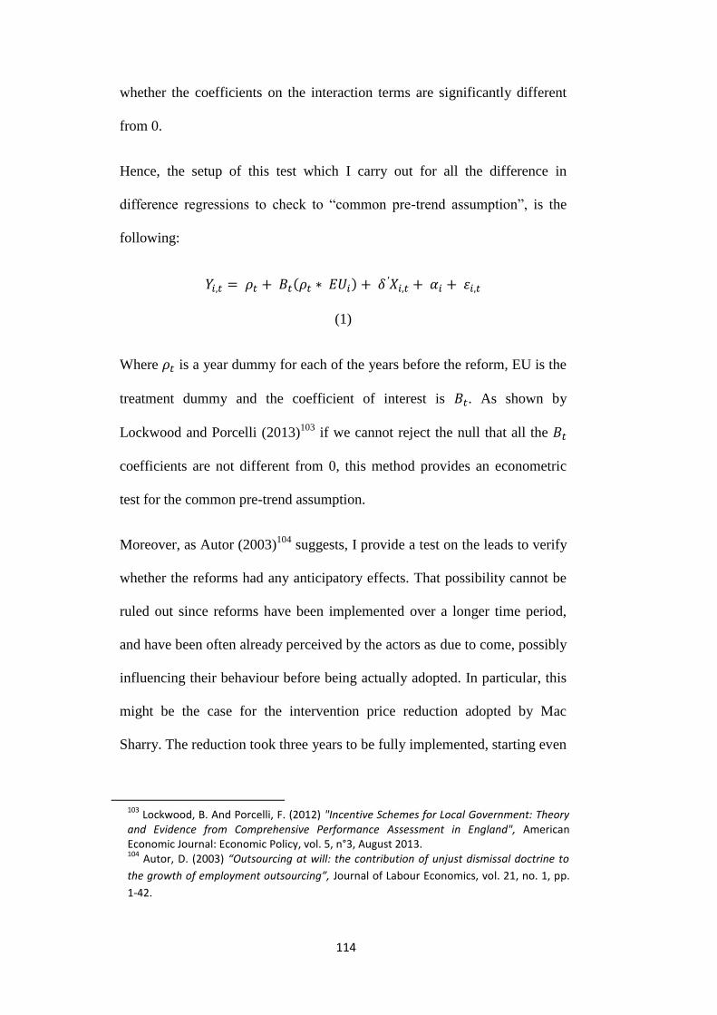
114

whether the coefficients on the interaction terms are significantly different

from 0.

Hence, the setup of this test which I carry out for all the difference in

difference regressions to check to “common pre-trend assumption”, is the

following:

𝑌𝑖,𝑡 = 𝜌𝑡 + 𝐵𝑡(𝜌𝑡 ∗ 𝐸𝑈𝑖) + 𝛿 ′𝑋𝑖,𝑡 + 𝛼𝑖 + 휀𝑖,𝑡

(1)

Where 𝜌𝑡 is a year dummy for each of the years before the reform, EU is the

treatment dummy and the coefficient of interest is 𝐵𝑡. As shown by

Lockwood and Porcelli (2013)103

if we cannot reject the null that all the 𝐵𝑡

coefficients are not different from 0, this method provides an econometric

test for the common pre-trend assumption.

Moreover, as Autor (2003)104

suggests, I provide a test on the leads to verify

whether the reforms had any anticipatory effects. That possibility cannot be

ruled out since reforms have been implemented over a longer time period,

and have been often already perceived by the actors as due to come, possibly

influencing their behaviour before being actually adopted. In particular, this

might be the case for the intervention price reduction adopted by Mac

Sharry. The reduction took three years to be fully implemented, starting even

103

Lockwood, B. And Porcelli, F. (2012) "Incentive Schemes for Local Government: Theory and Evidence from Comprehensive Performance Assessment in England", American Economic Journal: Economic Policy, vol. 5, n°3, August 2013. 104

Autor, D. (2003) “Outsourcing at will: the contribution of unjust dismissal doctrine to

the growth of employment outsourcing”, Journal of Labour Economics, vol. 21, no. 1, pp.

1-42.

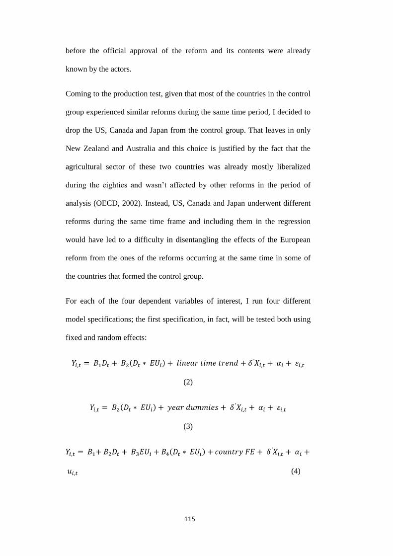
115

before the official approval of the reform and its contents were already

known by the actors.

Coming to the production test, given that most of the countries in the control

group experienced similar reforms during the same time period, I decided to

drop the US, Canada and Japan from the control group. That leaves in only

New Zealand and Australia and this choice is justified by the fact that the

agricultural sector of these two countries was already mostly liberalized

during the eighties and wasn’t affected by other reforms in the period of

analysis (OECD, 2002). Instead, US, Canada and Japan underwent different

reforms during the same time frame and including them in the regression

would have led to a difficulty in disentangling the effects of the European

reform from the ones of the reforms occurring at the same time in some of

the countries that formed the control group.

For each of the four dependent variables of interest, I run four different

model specifications; the first specification, in fact, will be tested both using

fixed and random effects:

𝑌𝑖,𝑡 = 𝐵1𝐷𝑡 + 𝐵2(𝐷𝑡 ∗ 𝐸𝑈𝑖) + 𝑙𝑖𝑛𝑒𝑎𝑟 𝑡𝑖𝑚𝑒 𝑡𝑟𝑒𝑛𝑑 + 𝛿 ′𝑋𝑖,𝑡 + 𝛼𝑖 + 휀𝑖,𝑡

(2)

𝑌𝑖,𝑡 = 𝐵2(𝐷𝑡 ∗ 𝐸𝑈𝑖) + 𝑦𝑒𝑎𝑟 𝑑𝑢𝑚𝑚𝑖𝑒𝑠 + 𝛿 ′𝑋𝑖,𝑡 + 𝛼𝑖 + 휀𝑖,𝑡

(3)

𝑌𝑖,𝑡 = 𝐵1+ 𝐵2𝐷𝑡 + 𝐵3𝐸𝑈𝑖 + 𝐵4(𝐷𝑡 ∗ 𝐸𝑈𝑖) + 𝑐𝑜𝑢𝑛𝑡𝑟𝑦 𝐹𝐸 + 𝛿 ′𝑋𝑖,𝑡 + 𝛼𝑖 +

𝑢𝑖,𝑡 (4)

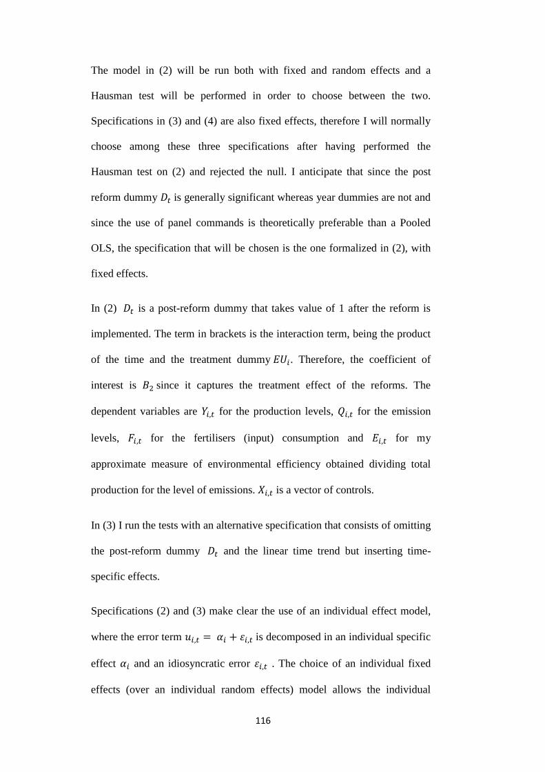
116

The model in (2) will be run both with fixed and random effects and a

Hausman test will be performed in order to choose between the two.

Specifications in (3) and (4) are also fixed effects, therefore I will normally

choose among these three specifications after having performed the

Hausman test on (2) and rejected the null. I anticipate that since the post

reform dummy 𝐷𝑡 is generally significant whereas year dummies are not and

since the use of panel commands is theoretically preferable than a Pooled

OLS, the specification that will be chosen is the one formalized in (2), with

fixed effects.

In (2) 𝐷𝑡 is a post-reform dummy that takes value of 1 after the reform is

implemented. The term in brackets is the interaction term, being the product

of the time and the treatment dummy 𝐸𝑈𝑖. Therefore, the coefficient of

interest is 𝐵2 since it captures the treatment effect of the reforms. The

dependent variables are 𝑌𝑖,𝑡 for the production levels, 𝑄𝑖,𝑡 for the emission

levels, 𝐹𝑖,𝑡 for the fertilisers (input) consumption and 𝐸𝑖,𝑡 for my

approximate measure of environmental efficiency obtained dividing total

production for the level of emissions. 𝑋𝑖,𝑡 is a vector of controls.

In (3) I run the tests with an alternative specification that consists of omitting

the post-reform dummy 𝐷𝑡 and the linear time trend but inserting time-

specific effects.

Specifications (2) and (3) make clear the use of an individual effect model,

where the error term 𝑢𝑖,𝑡 = 𝛼𝑖 + 휀𝑖,𝑡 is decomposed in an individual specific

effect 𝛼𝑖 and an idiosyncratic error 휀𝑖,𝑡 . The choice of an individual fixed

effects (over an individual random effects) model allows the individual

117

specific, time invariant, effects 𝛼𝑖 to be correlated with the regressors in 𝑋𝑖,𝑡,

allowing a partial endogeneity between the dependent variable and

regressors. The choice of a fixed over a random effects model can be

defended theoretically arguing that since the analysis is based on a panel of

countries, it is likely that each country might have specific characteristics

that are correlated with the regressors and, hence, with the dependent

variable. The assumption of the random effect model, in fact, states that the

individual effects are completely random, which would be difficult to defend

in this kind of setup. To overcome this model specification choice, however,

I will perform Hausman tests to choose between a fixed effects and a

random effects model.

The choice of specification (2), which as anticipated will be the preferred

one to perform the difference-in-difference estimator, has been taken looking

at Lockwood and Porcelli (2013). In particular, it allows the omission of the

treatment dummy from the regression; this is fundamental given my choice

to use a fixed effects model, which is in fact unable to estimate time

unvarying regressors such as the treatment dummy 𝐸𝑈𝑖,𝑡 in the present

specification.

Specification (4) provides a different estimator, a pooled OLS where

country/commodity fixed effects will be inserted as regressors. Therefore,

the difference with the specification proposed before would be minimal:

instead of using a fixed effect model I run a pooled OLS inserting country

fixed effects as regressors in the model.

118

In this specification, 𝐵1 is the coefficient for the control group pre-reform,

𝐵1+ 𝐵2 for the control group post-reform; 𝐵1+ 𝐵3 is the coefficient for the

treatment group pre-reform whereas 𝐵1+ 𝐵2 + 𝐵3+ 𝐵4 is the coefficient for

the treatment group post-reform. Therefore the difference-in-difference

estimator is derived as follows.

(𝑇𝑟𝑒𝑎𝑡𝑚𝑒𝑛𝑡𝑝𝑜𝑠𝑡 − 𝑇𝑟𝑒𝑎𝑡𝑚𝑒𝑛𝑡𝑝𝑟𝑒) − (𝐶𝑜𝑛𝑡𝑟𝑜𝑙𝑝𝑜𝑠𝑡 − 𝐶𝑜𝑛𝑡𝑟𝑜𝑙𝑝𝑟𝑒) = 𝐵4 (5)

To sum up, for each of the econometric test I will provide 4 different

estimators:

a fixed effects model that includes a post-reform dummy and a time trend

in the controls;

a fixed effect model without the post reform dummy and the linear time

trend but with the allowance of year dummies in the controls to isolate time-

fixed effects;

a pooled OLS with fixed effects included in the regression;

and a random effects model with the same features as the fixed effects

model in (2).

Regarding the accuracy of the estimates, these individual effects estimators

are based on the assumption that the idiosyncratic error 휀𝑖,𝑡 is ~ (0 , 𝜎𝜀2),

whereas this assumption is likely not to hold in panel applications. Hence, it

is necessary to compute cluster-robust standard errors (Bertrand et. al. 2004).

Without this correction, estimated standard errors would be incorrectly

underestimated, giving results that may appear significant even if they are

not when using the correct, cluster-robust, standard errors.

119

Before moving to the empirical analysis, it has to be clarified that since my

intent is to test two different reforms on the same sample, I have to run the

regressions for the Mac Sharry reform on a subsample that terminates the

year before the implementation of the second reform. Otherwise, the

coefficient on the interaction term would include the effects of the second

reform as well.

Coming to the valuation of the second reform, it is clear that the use of a

difference in difference estimator would be inadequate. In fact, given that the

common trend assumption held for the period before the first reform, if that

reform was effective and changed the trend, there would no longer be a

common trend assumption for the second reform. Therefore, instead of

running a regression including just the interaction term for the Fischler

reform, which would result in a biased estimation for the reason

aforementioned, I propose to include another interaction term, for the

Fischler reform, in the same regressions used to test the Mac Sharry’s one

but this time on the entire time period, keeping to use the same four model

specifications. As an example, the model in (2) would be specified as

follows:

𝑌𝑖,𝑡 = 𝐵1𝐷𝑀𝑎𝑐𝑆ℎ𝑎𝑟𝑟𝑦 + 𝐵2(𝐷𝑀𝑎𝑐𝑆ℎ𝑎𝑟𝑟𝑦 ∗ 𝐸𝑈𝑖) + 𝐵3𝐷𝐹𝑖𝑠𝑐ℎ𝑙𝑒𝑟 +

𝐵4(𝐷𝐹𝑖𝑠𝑐ℎ𝑙𝑒𝑟 ∗ 𝐸𝑈𝑖) + 𝑙𝑖𝑛𝑒𝑎𝑟 𝑡𝑖𝑚𝑒 𝑡𝑟𝑒𝑛𝑑 + 𝛿 ′𝑋𝑖,𝑡 + 𝛼𝑖 + 휀𝑖,𝑡

(6)

This estimator, hence, should be considered as an estimate of a

reinforcement (or attenuation) of the effects of the first reform and not

analysed individually. In other words, econometrically, it will be treated as if

120

it was a lag of the first reform, following the work of Autor (2003). Once the

common trend assumption for the years before the first reform has been

verified and the test for Mac Sharry performed on the appropriate

subsample, running the model in (6) on all time periods gives an estimate of

the second reform (𝐵4). For instance, assuming to have a negative 𝐵2 and 𝐵4

we would interpret 𝐵4 as a further reduction, whereas to have an overall

measure of the difference-in-difference estimator between treatment and

control group after the second reform, we should add the two coefficients of

the interaction terms.

121

2.3 Empirical analysis and results

Mac Sharry reform

The literature about the CAP reform process has focused on a variety of

specific aspects, as well as on broad empirical analysis. The present research

follows the second type of approach, seeking to provide an overall analysis

of the aggregate changes in the patterns of production, GHG emissions,

input use and an ad hoc measure of environmental efficiency. An obvious

limit will be the difficulty to disentangle the specific determinants of the

(mostly) positive changes that occurred. In fact, we will see that even finding

statistically significant results, the fact that the two reforms analysed

impacted on more than one single measure leads to some interpretational

issues in determining which particular reform contributed the most to the

overall achievement. However, it provides a useful tool to develop a broad

critical assessment of the overall reform process, providing empirical results

to judge the general effectiveness of the reforms.

Starting from the critique of what has been defined the ‘old’ CAP; most

experts agree that the high level of ‘coupled’ price intervention resulted in

the intensification and concentration of production responsible for the

overproduction problem and the deterioration of the environment in terms of

loss of biodiversity, soil erosion and GHG emissions (Baldock, 1990)105

.

105

D. Baldock (1990) “Agricultural and habitat loss in Europe”, World Wild Fund for Nature, London, 1990.

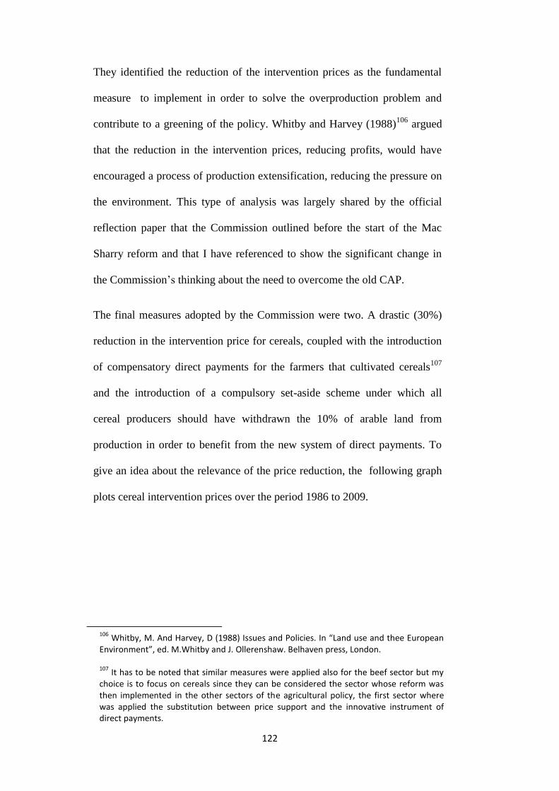
122

They identified the reduction of the intervention prices as the fundamental

measure to implement in order to solve the overproduction problem and

contribute to a greening of the policy. Whitby and Harvey (1988)106

argued

that the reduction in the intervention prices, reducing profits, would have

encouraged a process of production extensification, reducing the pressure on

the environment. This type of analysis was largely shared by the official

reflection paper that the Commission outlined before the start of the Mac

Sharry reform and that I have referenced to show the significant change in

the Commission’s thinking about the need to overcome the old CAP.

The final measures adopted by the Commission were two. A drastic (30%)

reduction in the intervention price for cereals, coupled with the introduction

of compensatory direct payments for the farmers that cultivated cereals107

and the introduction of a compulsory set-aside scheme under which all

cereal producers should have withdrawn the 10% of arable land from

production in order to benefit from the new system of direct payments. To

give an idea about the relevance of the price reduction, the following graph

plots cereal intervention prices over the period 1986 to 2009.

106

Whitby, M. And Harvey, D (1988) Issues and Policies. In “Land use and thee European Environment”, ed. M.Whitby and J. Ollerenshaw. Belhaven press, London. 107

It has to be noted that similar measures were applied also for the beef sector but my choice is to focus on cereals since they can be considered the sector whose reform was then implemented in the other sectors of the agricultural policy, the first sector where was applied the substitution between price support and the innovative instrument of direct payments.

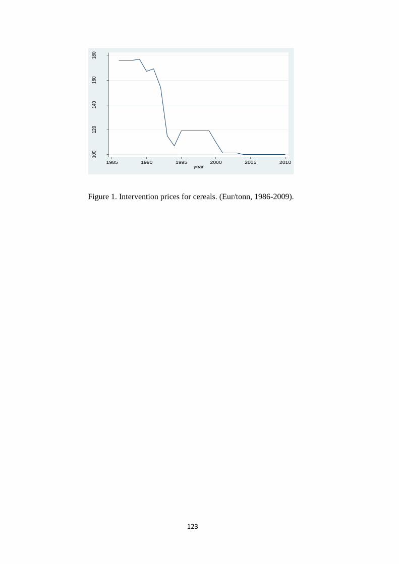
123

Figure 1. Intervention prices for cereals. (Eur/tonn, 1986-2009).

100

120

140

160

180

Inte

rven

tion

Pric

e

1985 1990 1995 2000 2005 2010year

124

The effects of the Mac Sharry reform are evident: intervention prices

progressively decrease from 169 Euro per ton in 1991 to 154 Euro/ton in

1992, 115 Euro/ton in 1993 and 107 Euro/ton in 1994, before being

increased to 119 Euro/ton in 1995.

The reduction of the intervention prices would reverse the perverse

mechanism highlighted by Potter (1996)108

who states that high intervention

prices induced farmers to maximize production by increasing the amount of

arable land and, since land supply is fixed, by intensifying the production

process increasing the use of fertilisers and pesticides, with obvious

repercussions in terms of environmental damage. Other scholars have argued

in favour of a double dividend (Jenkins, 1990)109

from agricultural

liberalisation: reducing intervention prices would both decrease

intensification and free resources for direct payments partially or totally

decoupled from production or even for environmental schemes designed to

address market failures. Moreover, that could be done at a lower expense for

the European citizens who would still bear the burden of the policy as

taxpayers, but would now have tangible benefits as consumers in terms of

food-price reductions. However, Potter and Goodwin (1998)110

provide a

critical assessment of these assumptions, highlighting the potential limits of

the argument that the reduction of the intervention prices and their

108

Potter, C. (1996), “Decoupling by degrees? Agricultural Liberalisation and its Implication for Nature Conservation in Britain”, English Nature Research Reports no. 196, Peterborough. 109

Jenkins, T. (1990), “Future harvester: the economics of Farming and the Environment”, Council for the protection of rural England, London 110

Potter, C. and Goodwin, P. (1998),“Agricultural liberalization in the European Union: An Analysis of the Implications for Nature Conservation”, Journal of rural studies, vol. 14, no. 3, pp 287-298.

125

substitution with direct payments would be the major driver for a greening of

the CAP. In particular, the authors claim that without an explicit “green”

recoupling of the alternative measures introduced, the effects of the price

liberalisation would not be automatically positive for the environment;

instead, the effect would be ambiguous. They conclude their analysis

arguing that the green recoupling needed to achieve the double dividend has

not been implemented sufficiently. On the basis of the share of the different

measures post Mac Sharry (43% for direct payment, 53% still in MPS and

just 4% in AEP) they observe that the resources freed by price reductions

basically resulted in direct payments still partially coupled with production,

hence inefficient in their ‘liberalising’ purpose and that, moreover, they

haven’t been used to create agri-environmental (AEP) schemes to address

market failure.

Coming to the other main measure introduced by the Mac Sharry reform, the

set-aside was originally thought to address the overproduction problem.

However, its link with the environment is straightforward since it basically

triggered (for the cereal producers) a withdrawal of almost 10% of the arable

land from production. A recent paper (IEEP, 2008)111

summarises the

benefits produced by set-aside since its introduction as a voluntary measure

in 1988. It provides evidence regarding the reduced use of herbicides,

fungicides, insecticides and molluscicides on set-aside land in comparison

with rape and wheat cultivation. The contribution of set-aside to reducing

GHG emission has not been object of many studies but the theoretical

111

IEEP (2008), “The Environmental Benefits of Set-Aside in the EU: a summary of evidence”, Prepared by The Institute for European Environmental Policy for Department for the Environment, Food and Rural Affairs , February 2008.

126

argument is normally that the removal of atmospheric CO2 would come

from plants, which would also store the fixed carbon as soil organic matter,

and would be a logical consequence of having less land under cultivation.

However, as anticipated before, a limit of the capacity of this measure to

address the environmental externalities created by the old CAP and the

overuse of chemicals is that the farmers could now decide to apply a greater

amount of input on the reduced amount of land under cultivation, with the

consequence that the overall, positive, effect on emission could be

minimized if not cancelled.

This brief analysis of the literature regarding the Mac Sharry reform

identifies two main measures that might have had an impact on the

environment and production: the reduction in intervention prices and the set-

aside. The predicted effects are a (relative) reduction in cereal crops, a

reduction in input used due to the ‘extensification effect’ promoted by price

cuts and by the set-aside itself and a reduction in the amount of GHG.

Josling (1994) have also claimed that the reduction in intervention prices has

increased market exposure, leading farmers to take production decisions on

the basis of the international prices. However, the test regarding the

effectiveness of the reforms to determine a shift in the way farmers took

their production decision will be done in the next section, when the Fischler

reform will be taken into account. In fact, since the payments introduced by

Mac Sharry were not fully decoupled it makes more sense to carry out an

analysis on the complete time period and verify whether international prices

became significant only after the full decoupling was introduced or whether

the Mac Sharry reform was enough to trigger this change in farmers

127

behaviour, from producing to the intervention agencies to producing for the

market.

128

Mac Sharry reform: Effects on production.

Starting with the regression on production levels, the control group is formed

only by Australia and New Zealand following the work of Legg (OECD,

2002)112

, who showed that Canada, Japan and the US proceeded with similar

reforms in the same time period. Hence, results using these countries might

be biased because they are unable to take into account the effects of these

other reforms happening at the same time. Therefore, the choice to exclude

those countries is made in order to have a control group composed by

countries that have not experienced other reforms in the same time period;

moreover, having largely liberalised years before the reform under

consideration, these two countries would represent a quite stabilized free

trade scenario that will be used as a reference point for the evaluation of the

two reforms.

For the test of the Mac Sharry reform, I use a subsample that ends in 2005 in

order to avoid the inclusion of the effects of the Fischler reform,

implemented in 2006. As shown in Figure 2, production (in thousand tons)

of three different cereals has been regressed over the Mac Sharry interaction

term and a set of controls: prices, fertiliser consumption, GDP per capita. In

the first specification (linear time trend plus post-reform dummy) the

interaction term shows a negative and significant coefficient as predicted,

and so does the second model, with year dummies to isolate time-fixed

112

Legg, W. (2002) “The evolution of agricultural policies in OECD countries as reflected by the level and structure of agricultural support” in “China in the Global Economy Agricultural Policies in China after WTO Accession”, OECD.

129

effects. The pooled OLS estimator with country fixed effects inserted as

regressors shows similar results and so does the random effects model with

the post-reform dummy and the linear trend.

Figure 2. Production regression on levels for Mac Sharry reform.

FE Pooled OLS RE

(1) (2) (3) (4)

Post & Trend Time FE Post Post

prices -1.939 -0.697 -2.248 -1.719

(2.649) (3.811) (2.885) (2.532)

Mcsharry -1586.7** -1641.6** -1662.5** -1197.5

(734.5) (729.1) (765.6) (769.4)

gdpcapita 0.0307 0.0418 0.0642* 0.0359

(0.0645) (0.0704) (0.0367) (0.0694)

fertcons -0.360 -0.521 -0.394 -0.0240

(0.491) (0.518) (0.529) (0.411)

EU 9930.5***

(546.4)

Time FE No Yes No No

Post

Reform

Yes No Yes Yes

Trend Yes No No Yes

Country/C

ommodity

FE

No No Yes No

N 660 660 660 660

Standard errors in parentheses * p<0.1, ** p<0.05, *** p<0.01

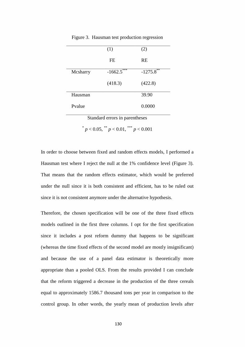
130

Figure 3. Hausman test production regression

(1) (2)

FE RE

Mcsharry -1662.5***

-1275.8**

(418.3) (422.8)

Hausman 39.90

Pvalue 0.0000

Standard errors in parentheses

* p < 0.05,

** p < 0.01,

*** p < 0.001

In order to choose between fixed and random effects models, I performed a

Hausman test where I reject the null at the 1% confidence level (Figure 3).

That means that the random effects estimator, which would be preferred

under the null since it is both consistent and efficient, has to be ruled out

since it is not consistent anymore under the alternative hypothesis.

Therefore, the chosen specification will be one of the three fixed effects

models outlined in the first three columns. I opt for the first specification

since it includes a post reform dummy that happens to be significant

(whereas the time fixed effects of the second model are mostly insignificant)

and because the use of a panel data estimator is theoretically more

appropriate than a pooled OLS. From the results provided I can conclude

that the reform triggered a decrease in the production of the three cereals

equal to approximately 1586.7 thousand tons per year in comparison to the

control group. In other words, the yearly mean of production levels after

131

1993 for the treatment group, is 1586.7 thousand tons lower than what it

would have been without the reform, since it would have followed the same

(higher) increasing trend observed in the control group.

The next test follows Autor (2003) in the attempt to test for anticipatory

effects. Taking the first of the four models presented, I include three leads of

the interaction term and three pre-reform dummies for the three years before

reform’s implementation. To check for anticipatory effects we have to look

at the coefficients of the leads of the interaction term. As reported Figure 4,

an anticipatory effect was present in 1992 and this is not surprising as the

intervention prices were reduced from 169 Euro/ton to 154 Euro/ton in 1992.

Instead, there is no evidence for anticipatory effects before 1992. It has to be

mentioned that a voluntary set aside was already part of the CAP since 1988;

hence, an anticipatory effect in 1992 might be the result of an increasing use

of the voluntary set aside scheme, combined with the decrease in the

intervention prices, with this final factor being, likely, the main driver.

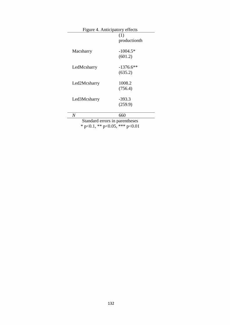
132

Figure 4. Anticipatory effects

(1)

productionth

Macsharry -1004.5*

(601.2)

LedMcsharry -1376.6**

(635.2)

Led2Mcsharry 1008.2

(756.4)

Led3Mcsharry -393.3

(259.9)

N 660

Standard errors in parentheses

* p<0.1, ** p<0.05, *** p<0.01

133

To conclude the analysis of the effects on production, the common trend

assumption has to be verified. Figure 5 presents a graph for the trends in

treatment and control group before and after the reform113

. Admittedly, the

graph is not very useful to see whether the two groups followed a common

trend before the reform; hence I proceed with an econometric test following

equation (1). However, what seems clear from the graph is that the

difference between treatment and control group is decreasing over time (note

that the mean of production was higher for the treatment group), due to a

slower increase of the production levels in Europe in comparison with the

control group. Hence, interpreting equation (5), the diff-in-diff estimator

gives a negative and significant coefficient. In other words, we expect that

without the reform the production levels for the treatment group would have

increased more, keeping almost the same spread with the control group,

instead of reducing it.

113

Here, g1y0 stands for the treatment group, whereas g2y0 indicates the control group. Moreover, the plot points that they represent are not individual data point but are the weighted average of production levels of the countries that form, respectively, the treatment and the control group.

134

Figure 5. Common trend assumption. Graph analysis.

The results of the econometric test for the pre-reform common trend

assumption are in Figure 6. Given that the policy started in 1993, the null

hypothesis is that 𝐵𝑡 = 0 for each time period between 1986 and 1993

(excluded) and it cannot be rejected apart from 1988. Therefore, it could be

argued that the use of the difference-in-difference estimator is appropriate

and that it validates the theoretical prediction that the Mac Sharry reform

was effective in triggering a (relative) decrease in the production levels in

comparison with the scenario that would have happened in absence of the

reform. Finally, I believe that the anticipatory effect registered in 1992,

when the compulsory set aside had not been introduced yet and just a partial

cut in the intervention price took place, might be the proof that the real

driver of this relative decrease in production has been mainly the cut in the

intervention prices, validating the predictions of Whitby and Harvey (1988)

and Potter (1996).

2000

3000

4000

5000

6000

7000

1985 1990 1995 2000 2005

g1y0 treat. group g2y0 contr. group Fitted values Fitted values Fitted values Fitted values

135

Figure 6. Common trend assumption. Econometric test.

(FE)

productionth

int1987 753.0

(575.7)

int1988 820.1*

(406.2)

int1989 524.4

(488.5)

int1990 189.4

(452.3)

int1991 1252.0

(1120.2)

int1992 -85.14

(621.7)

N 231

Standard errors in parentheses

* p<0.05, ** p<0.01, *** p<0.001

136

Mac Sharry reform: Effects on emissions

Before presenting the results of the emissions regression I would like to

clarify the importance of having a good estimate of these data. Indeed, since

I am also analyzing the reform’s effects on production, it might be that the

results on emissions are simply a linear transformation of the ones on

production. In other words, if emissions from agriculture were simply

estimated applying a conversion coefficient to the amount of agricultural

goods produced it is trivial to say that performing an analysis on emissions

would be redundant.

The data come from the FAOSTAT database, in which it is included an

estimate of the emissions occurring from agriculture. Tubiniello et all

(2013)114

present their methodology, clarifying the use of a bottom-up

approach based mainly on the use of a combination of crop area (number of

livestock), activity type and an activity- specific emission conversion

factors. In other words, each different production type was allocated an

emission factor also considering the geographic location of the country (in

order to have an approximate distinction between developed and developing

countries) and the national emission data from agriculture was computed as

the sum of each estimate for each single type of production. Also the use of

synthetic fertilisers was included in the analysis with the aim of providing an

overall assessment of the level of production intensity.

114

Tubiniello et all, “The FAOSTAT database of greenhouse gas emissions from agriculture”, Environmental Research letters, 2013, issue 8.

137

In my opinion the methodology followed guarantees a substantial

independence between the measure of agricultural production and the

estimate of total emissions. First of all, the emission factors are applied on

the area under cultivation. and not on total production.

Most importantly, there is no obvious direct link between the two. Indeed, it

might well be that production remains more or less constant even with a

reduction of a land under cultivation (if, for example, more fertilisers are

now applied on the diminished land under cultivation) whereas emission

decrease substantially (even if the use of fertilisers remains, again, fairly

similar) due to a simple decrease in the area under cultivation and the

extension of area under forestry or “environmental systems” such as buffer

strips.

More importantly, this measure allows to distinguish our emission estimates

from a simple transformation of total production if we consider weather’s

impact on production. Indeed, it might well be that for certain climatic

occurrences production would be boosted or hampered, regardless of the

production technique used. In other words, had we used a simple

transformation of total production in a particularly bad (or good) year we

would have ended up saying that emissions also decreased (or increased)

substantially in that particular year for that specific country. Instead, it is

extremely likely that this variations in production occurred regardless the

fact that the production technique was the same, with the same effects in

terms of emissions.

138

The authors underlie some limitations of their methodology, in particular the

considerable uncertainty (and wide confidence intervals) due to the choice of

using the same emission conversion factors at a regional level, with the

consequence of not being able to capture potentially substantial differences

in production intensity between countries within the same regional group.

However, or the purposes of the present analysis I believe that this

methodology is sufficiently different from the data on production to allow an

independent analysis of the emissions from agriculture.

Moreover, I have included a measure of total cereal production in my

regression model to test whether it is correlated with emissions and the

results seem to indicate that my assumption of independence was correct

since total production is not significant in all the three fixed effects models

tested (it is significant in the random effect model but we reject it after

having performed the Hausman test).

In this regression, the control group is composed of the five mentioned

countries. To test the Mac Sharry reform I run, over the same subsample, the

four aforementioned model specifications, the results of which are shown in

Figure 7.

The interaction term appears to be significant (although just at the 10%

level) and negative in all the four different models. As before, to choose

between fixed effects and random effects, I use both the theoretical argument

that states that a fixed effect model is more appropriate when analysing

countries and the econometric test performed with the Hausman test (Figure

8). I reject the null and therefore opt for a fixed effect model. The choice

139

between the three different fixed effects models is for the first one that

allows for a linear trend and includes a post reform dummy, since it happens

to be significant at the 10% level. Moreover, time specific effects in the

second specification are generally not significant and the choice of a panel

estimator is theoretically preferable to the Pooled OLS reported in column

three.

140

Figure 7. Emission regression in levels for Mac Sharry

FE Pool RE

(1) (2) (3) (4)

Post & Trend Time FE Post Post

fprice -0.00938 2.459 -0.250 -0.621

(1.099) (6.659) (1.041) (0.595)

Totalproduction 0.0537 0.0503 0.0548 0.152***

(0.0464) (0.0425) (0.0469) (0.0525)

Mcsharry -7189.6* -7210.5* -7200.7* -7245.2*

(3525.4) (3632.3) (3732.1) (3884.5)

gdpcapita 0.185 0.203 -0.0270 0.239

(0.213) (0.227) (0.112) (0.257)

avprecipitation 3469.9* 3464.0* 3580.3* 27.38*

(1711.2) (1655.8) (1783.9) (15.15)

EU 13709208.5*

(6846127.0)

Time FE No Yes No No

Post Reform Yes No Yes Yes

Trend Yes No No Yes

Country/Commo

dity FE

No No Yes No

N 240 240 240 240

Standard errors in parentheses

* p<0.1, ** p<0.05, *** p<0.01

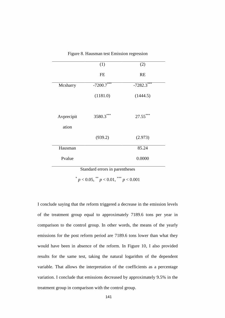
141

Figure 8. Hausman test Emission regression

(1) (2)

FE RE

Mcsharry -7200.7***

-7282.3***

(1181.0) (1444.5)

Avprecipit

ation

3580.3***

27.55***

(939.2) (2.973)

Hausman 85.24

Pvalue 0.0000

Standard errors in parentheses

* p < 0.05,

** p < 0.01,

*** p < 0.001

I conclude saying that the reform triggered a decrease in the emission levels

of the treatment group equal to approximately 7189.6 tons per year in

comparison to the control group. In other words, the means of the yearly

emissions for the post reform period are 7189.6 tons lower than what they

would have been in absence of the reform. In Figure 10, I also provided

results for the same test, taking the natural logarithm of the dependent

variable. That allows the interpretation of the coefficients as a percentage

variation. I conclude that emissions decreased by approximately 9.5% in the

treatment group in comparison with the control group.

142

Figure 10. Emission regressions for Mac Sharry in Logarithm (% change)

FE Pool RE

(1) (2) (3) (4)

Post & Trend Time FE Post Post

fprice -0.00000939 0.0000220 -0.0000112 -0.00000718

(0.0000119) (0.000145) (0.0000132) (0.0000103)

totalproductionth 0.00000104 0.000000934 0.00000104 0.000000899

(0.000000934) (0.000000887) (0.000000959) (0.000000621)

Mcsharry -0.0945* -0.0951* -0.0946* -0.0892*

(0.0448) (0.0459) (0.0463) (0.0469)

gdpcapita -0.00000148 -0.000000975 -0.00000309 -0.00000190

(0.00000523) (0.00000552) (0.00000300) (0.00000530)

avprecipitation -0.0214 -0.0214 -0.0206 0.000276***

(0.0428) (0.0418) (0.0442) (0.0000868)

EU -79.26

(169.7)

Time FE No Yes No No

Post Reform Yes No Yes Yes

Trend Yes No No Yes

Country/Commodi

ty FE

No No Yes No

N 240 240 240 240

Standard errors in parentheses

* p<0.1, ** p<0.05, *** p<0.01

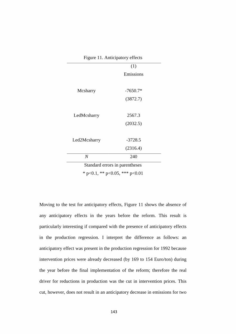
143

Figure 11. Anticipatory effects

(1)

Emissions

Mcsharry -7650.7*

(3872.7)

LedMcsharry 2567.3

(2032.5)

Led2Mcsharry -3728.5

(2316.4)

N 240

Standard errors in parentheses

* p<0.1, ** p<0.05, *** p<0.01

Moving to the test for anticipatory effects, Figure 11 shows the absence of

any anticipatory effects in the years before the reform. This result is

particularly interesting if compared with the presence of anticipatory effects

in the production regression. I interpret the difference as follows: an

anticipatory effect was present in the production regression for 1992 because

intervention prices were already decreased (by 169 to 154 Euro/ton) during

the year before the final implementation of the reform; therefore the real

driver for reductions in production was the cut in intervention prices. This

cut, however, does not result in an anticipatory decrease in emissions for two

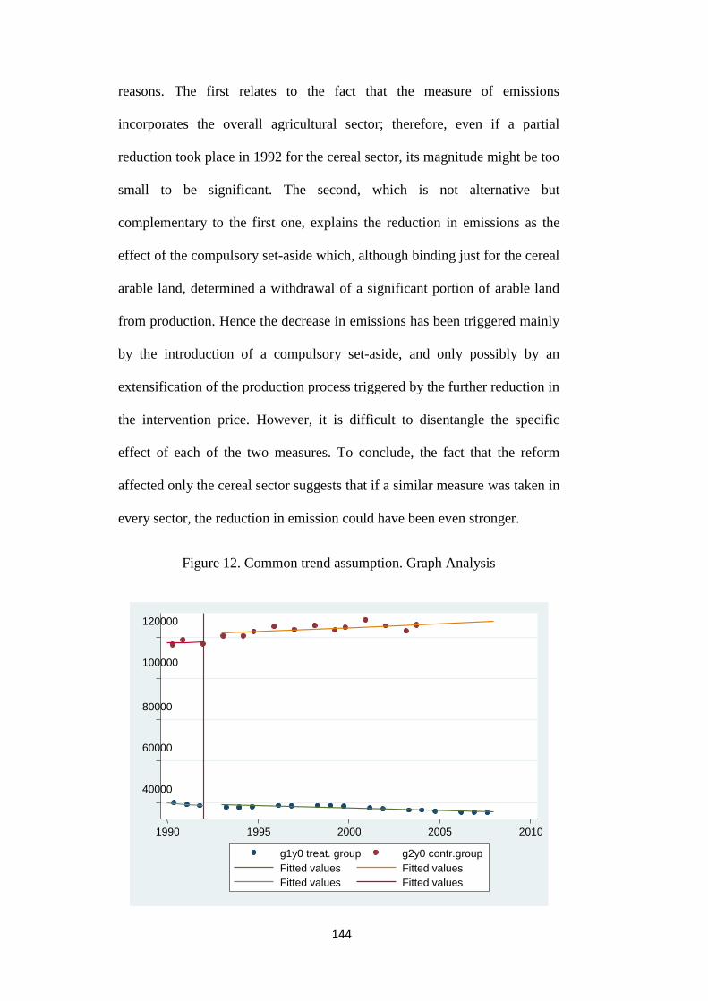
144

reasons. The first relates to the fact that the measure of emissions

incorporates the overall agricultural sector; therefore, even if a partial

reduction took place in 1992 for the cereal sector, its magnitude might be too

small to be significant. The second, which is not alternative but

complementary to the first one, explains the reduction in emissions as the

effect of the compulsory set-aside which, although binding just for the cereal

arable land, determined a withdrawal of a significant portion of arable land

from production. Hence the decrease in emissions has been triggered mainly

by the introduction of a compulsory set-aside, and only possibly by an

extensification of the production process triggered by the further reduction in

the intervention price. However, it is difficult to disentangle the specific

effect of each of the two measures. To conclude, the fact that the reform

affected only the cereal sector suggests that if a similar measure was taken in

every sector, the reduction in emission could have been even stronger.

Figure 12. Common trend assumption. Graph Analysis

40000

60000

80000

100000

120000

1990 1995 2000 2005 2010

g1y0 treat. group g2y0 contr.group Fitted values Fitted values Fitted values Fitted values

145

Figure 13. Common trend assumption. Econometric test

(1)

Emissions

int1990 4626.2

(2978.0)

int1991 2883.9

(1696.9)

int1992 1678.8

(1303.3)

N 60

Standard errors in parentheses

* p<0.1, ** p<0.05, *** p<0.01

Finally, figure 12 shows the graph for the common trend assumption before

the reform, whereas figure 13 provides the results of the econometric test

specified in equation (1)115

. It seems that the common trend assumption pre

reform holds and that, after the reform, emissions start to increase for the

control group, whereas they decrease for the treatment group. The

econometric test confirms these results, substantially validating the common

trend assumption pre-reform since all the coefficients on the 𝐵𝑡 coefficient in

(1) are insignificant. Therefore, the use of a difference-in-difference

estimator seems to be appropriate and validates the prediction that the Mac

115

As before, g1y0 expresses the weighted average of emissions levels for the treatment group, whereas g2y0 provides the same measure for the control group.

146

Sharry reform, through the reduction of intervention prices and, mainly,

through the adoption of a set-aside scheme, was effective in reducing the

GHG emissions for the overall agricultural sector.

147

Mac Sharry reform: effects on input use and environmental efficiency

Coming to the effects of Mac Sharry’s reform on input use, the theoretical

arguments suggested that this might have occurred as a consequence of both

the reduction in the intervention prices (and the consequent extensification

of the productive system) and the introduction of the set aside that suddenly

implied the withdrawal of a consistent proportion of arable land from

productive use. However, as reported in the IEEP paper (2008) the set aside

might have determined a parallel increase in input use on the residual arable

land, with an ambiguous overall effect.

Figure 15 shows the result of the main regression and all the four models

show a negative and significant coefficient for the interaction term.

However, as the graph in figure 16 suggests116

, the common trend

assumption before the reform does not hold. The econometric test in figure

17 shows that the 𝐵𝑡 coefficients before 1993 are not equal to 0. Therefore,

the difference-in-difference estimator leads to biased estimates and cannot be

used to test the effects of the reform.

116

g1y0 expresses the weighted average of fertilisers’ consumption for the treatment group, whereas g2y0 provides the same measure for the control group.

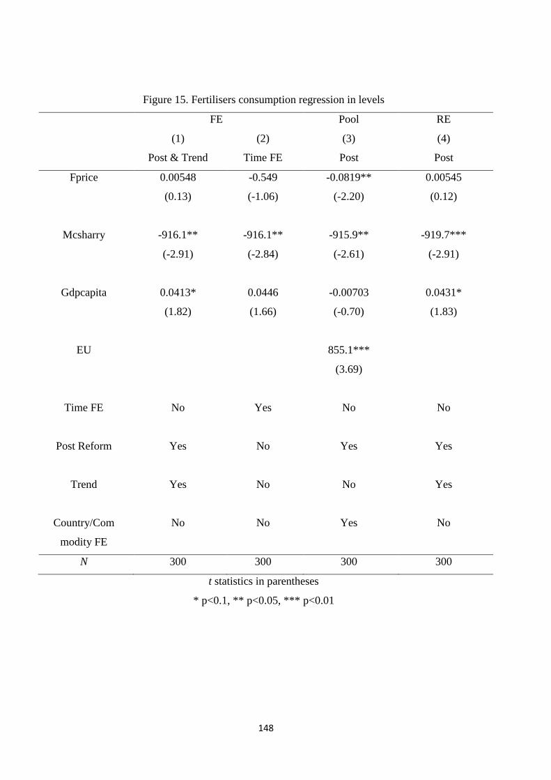
148

Figure 15. Fertilisers consumption regression in levels

FE Pool RE

(1) (2) (3) (4)

Post & Trend Time FE Post Post

Fprice 0.00548 -0.549 -0.0819** 0.00545

(0.13) (-1.06) (-2.20) (0.12)

Mcsharry -916.1** -916.1** -915.9** -919.7***

(-2.91) (-2.84) (-2.61) (-2.91)

Gdpcapita 0.0413* 0.0446 -0.00703 0.0431*

(1.82) (1.66) (-0.70) (1.83)

EU 855.1***

(3.69)

Time FE No Yes No No

Post Reform Yes No Yes Yes

Trend Yes No No Yes

Country/Com

modity FE

No No Yes No

N 300 300 300 300

t statistics in parentheses

* p<0.1, ** p<0.05, *** p<0.01

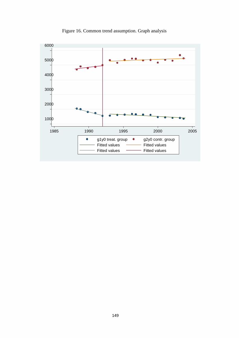
149

Figure 16. Common trend assumption. Graph analysis

1000

2000

3000

4000

5000

6000

1985 1990 1995 2000 2005

g1y0 treat. group g2y0 contr. group

Fitted values Fitted values

Fitted values Fitted values

150

Figure 17. Common trend assumption. Econometric test

(1)

Fertcons

int1987 -187.5*

(99.15)

int1988 -138.8

(110.9)

int1989 -396.2

(289.5)

int1990 -436.1

(332.4)

int1991 -561.5

(377.5)

int1992 -875.0*

(424.8)

fprice 1.089

(1.083)

gdpcapita -0.0913

(0.143)

N 105

Standard errors in parentheses

* p<0.1, ** p<0.05, *** p<0.01

151

To conclude, the only fact that seems evident from a simple graph analysis is

that, whereas the input use had been constantly increasing in the control

group, the treatment group had experienced a significant decrease from the

beginning of the time period. However, there is no empirical evidence of any

effect of the reform on the input use. Coming back to our theoretical

hypothesis this particular feature could be the result of the phenomenon I

described above as a potential counteracting force with respect to input

reductions. On the one hand we have said that both price reduction and the

compulsory set aside should have decreased input use. On the other hand it

might be the case that the farmers increased the level of input use on the land

still under cultivation with an overall reduction too small to be statistically

significant and captured by the model.

152

Moving to the analysis of our measure of environmental inefficiency, I

constructed an approximate measure of ‘environmental efficiency’ that

consists in dividing total agricultural production (in tons) by emissions (in

tons) I followed the aforementioned methodology to investigate the effects

of both the reforms. However, as Figure 18 and 19 show the common trend

assumption does not hold either before 1993, or before 2006117

. Hence, a

simple graph analysis depicts that a difference-in-difference estimator would

lead to biased estimates and the results would not be presented since they

would be theoretically inaccurate. It is still possible, however, draw some

conclusions looking at the trend in both the treatment and in the control

group. Particularly, it seems that my measure of efficiency has constantly

increased over the last 20 years for the 10 European countries analysed:

emissions have decreased substantially whereas the total production

remained stable or even increased (as reported for the cereal sector),

resulting in an overall increase of efficiency. On the other hand, this measure

of efficiency has been substantially stable in the control group, suggesting

that the reforms that occurred in the European Union might have had a

positive effect in boosting efficiency. Indeed, had we observed a similar

raise in efficiency also in the control group it would have been more logical

to find its reason in some factor (like for example a new and better fertiliser

or a new production technique) that affected cereal production across the

world; the fact that this measure of efficiency grows only in the EU, instead,

seems to suggest an impact of the reform.

117

g1y0 expresses the weighted average of my measure of ‘environmental efficiency’ for the treatment group, whereas g2y0 provides the same measure for the control group.

153

Figure 18. Testing the common trend assumption for Mac Sharry.

Figure 19. Testing the common trend assumption for Fischler.

700

800

900

1000

1990 1995 2000 2005 2010

g1y0 treat. group g2y0 contr. group Fitted values Fitted values Fitted values Fitted values

700

800

900

1000

1990 1995 2000 2005 2010

g1y0 treat. group g2y0 contr. group Fitted values Fitted values Fitted values Fitted values

154

Fischler reform

As regards the Fischler reform, approved in 2003 and finally implemented in

2006, its main changes consist in an attempt to fully decouple the direct

payments under the first pillar of the CAP and in the introduction of

environmental standards to be respected in order to receive the payments

(cross-compliance).

As anticipated, the reform of the direct payments and the introduction of the

Single Payment Scheme was meant to end the link between the level of

subsidy and the current type of production. Each European country had the

choice between adopting an “historical” or a “regional” model for the

allocation of payments under the I pillar. Under the historical model every

payment per hectare depended on the amounts of payments received in the

reference period (2000-2002). Hence the level of payment per hectare was

already fixed and not affecting the production decisions in the present time.

Under the regional model a flat rate per hectare was fixed in every region

and therefore had no impact on the type of crop under cultivation.

Another main feature of the SPS was the introduction of GAEC118

standards

which subordinated the payments to the fulfilment of standards regarding

agricultural and environmental practice. Respecting GAEC standards was

the only condition for the reception of the payments. Hence, production was

not compulsory in order to benefit from the SPS. That was a main innovation

of the SPS that aimed at eliminating any form of distortions on production

118

Good Agro-Environmental Conditions.

155

decisions. Another expected effect of the introduction of GAEC standards is

a beneficial effect on some environmental indicators (especially water and

air quality and the level of greenhouse gas emissions, GHG) due to the

conditionality of SPS payments. However, as we will see from the literature

review on the environmental effects of the Fischler reform, decoupling

might trigger negative effects on some environmental public goods as

agricultural production declined on marginal land with potentially negative

effects in terms of management of the agricultural landscape, water systems

and fire and soil erosion prevention.

Literature review

Decoupling payments have been a major area of research in agricultural

economics in the last twenty years, as different countries tried to implement

policies which managed to fulfil the goal of sustaining farm incomes without

distorting production decisions. Regarding the CAP I described the

progression from price support to still partially coupled direct payments

(under Mac Sharry) to the fully decoupled payments under Fischler reform. I

will proceed providing some of the main findings of the recent literature on

the topic and then moving on to studies that directly examined the European

situation. Then, the main empirical findings of the present research will be

outlined an analysed in light of the findings in the existing literature.

156

Starting from the general literature about decoupled payment, as Beard and

Swinbank (2001)119

note, several nation introduced progressively more

decoupled payments starting from the early eighties and at least a partial

decoupling of national agricultural policy became a milestone of the

Uruguay round negotiations of the GATT. The idea was that in order to

liberalize trade in the agricultural sector, policies that created distortions on

production decisions and hence increase internal production artificially

would have had negative spill-overs on other nation via a reduction of the

international prices. The central assumption regarding decoupled direct

payments in fact was their ability not to influence production decisions.

Agricultural economists have faced the problem from both a theoretical and

an empirical perspective, finding contrasting results on both fields.

From a theoretical point of view there are at least three different

explanations of how decoupled direct payments could still affect production

decisions.

The first is the assumption that farmers might have a non-constant

(specifically decreasing in wealth) risk aversion.120

In particular, farmers are

assumed to be more inclined to make risky (but possibly more productive)

investments as their level of wealth increases. Hence, direct payment could

still boost production via a wealth effect as the farmer might undertake

investments that he wouldn’t have made in absence of the direct payments..

119

Beard, N., Swinbank,A. “Decoupled payments to facilitate CAP reform”, Food Policy 26 (2001). 120

Hennessy, D. A. 1998. The Production Effects of Agricultural Income Support Policies under Uncertainty. American Journal of Agricultural Economics 80(1): 46–57.

157

The second argument follows the assumption of imperfect credit markets

and credit constrained farmers. In such a situation an hypothetical farmer

willing to make a new productive investment might not be given the capital

required because of imperfect credit market. Direct payments would hence

enable farmers to sustain short term liquidity needs or undertake long term

investment. By increasing land values and the collateral they might ease the

credit constrain therefore allowing for greater investment and output.121

In

this scenario the payments help the farmer undertaking the investments both

directly and indirectly through the raise in land values and collateral that

would boost the farmer’s likelihood to be allowed a loan from a bank.

The third argument used to explain a potential production non-neutrality of

decoupled direct payments regards household labour allocation.122

The idea

is that getting more money would create the incentive for households to

decrease off-farm labour allocation and work more on their farm with the

predictable result of an increase in output.

Having clarified theoretically the potential channels though which decoupled

payments could still affect production, the empirical literature finds

contrasting results. For instance, Serra, Godwin and Featherstone (2011)123

find empirical evidence of risk aversion decreasing in wealth. On the other

hand, the estimated elasticity between direct payments and agricultural

output seems to be negligible, suggesting that the argument, even if valid

121

Roe, T., A. Somwaru, and X. Diao. 2003. Do Direct Payments Have Intertemporal Effects on US Agriculture? In Government Policy and Farmland Markets, ed. C. B. Moss and A. Schmitz 115–139. Ames, IA: Iowa State Press. 122

A. Hearn, M., El-Osta, H. and Dewbre, J. ‘The impact of coupled and decoupled government subsidies on off-farm labor participation of U.S. farm operators’, American Journal of Agricultural Economics, Vol. 88, (2006) pp. 393–408 123

Serra,T., B. K. Goodwin, and A. Featherstone. 2011. Risk Behavior in the Presence of Government Programs. Journal of Econometrics 162(1): 18–24.

158

from a theoretical point of view could not explain the non-neutrality of direct

payments on production, assuming that the phenomenon is actually real (and

measurable). A recent paper of Bakhshy and Gray (2012)124

analyses the

Canadian case and finds consistent acreage responses to the introduction of

decoupled payments, with consequent non-neutral effects on production.

Key et all (2005)125

analyse the US 1996 FAIR act comparing acreage and

farm size growth between farms participating or not in the federal

agricultural program; their result also suggest a positive production effect of

decoupled payments. On the other hand, Godwin and Misra (2006)126

results

on the effects of the FAIR act suggest that production effects, even if

positive and significant, are very modest and that probit estimations show

that decoupled payments do not influence the likelihood that farmers will

acquire more land.

Regarding the studies on decoupled payments in the European Union a

previous word of warning has to be spent since normally the objective of the

research is not to test whether the SPS still has production effects but

whether it reduced them in comparison with the pre-reform scenario. This

feature will characterize also my empirical tests on production and on

emission which in fact will have to be interpreted as a further reinforcement

of the negative effects on the two dependent variables already found for the

Mc Sharry reform.

124

Bakhshy, R. S. Gray ‘Acreage response to whole farm income stabilisation programs’ Journal of Agricultural Economics, Vol. 63, No. 2, 2012, 385–407 125

Key, N., R. N. Lubowski and M. J. Roberts, ‘Farm-level production effects from participation in government commodity programs: did the 1996 federal agricultural improvement and reform act make a difference?’ American Journal of Agricultural Economics, Vol. 87, (2005) pp. 1211-1219. 126

Goodwin, B. K. and A. K. Mishra. ‘Are “Decoupled” Farm Payments Really Decoupled? An Empirical Evaluation’. American Journal of Agricultural Economics Vol. 88(1), 2006: 73–89.

159

Gohin (2006) analyses whether the Fishler reform actually reduced

production incentives with respect to the previous, still partially coupled,

Mac Sharry payments. 127

His findings confirm that Fischler reform has

increased the level of decoupling of direct payments, decreasing the

production incentives with respect to the pre-reform scenario. Sckokai and

Moro (2009) analyse the effect of the introduction of the SPS in the arable

sector in terms of effects on farm investment and output.128

Using a sample

of Italian farms from the Farm Data Accountancy Network they find that,

contrary to changes in intervention prices, policy changes not affecting price

uncertainty (such as the SPS) do not have significant effects on production

and hence can be considered almost totally decoupled.

Regarding the Fischler’s reform effects on the environment, Schmid et al.

(2007) state that the reform attempted to phase out environmentally harmful

subsidies. However, it might be argued that the main scope of the further

‘decoupling’ was to induce farmers to take decisions based on market

signals, whereas the positive effect on the environment would have been

already included as a result of the Mac Sharry reform, being based on the

extensification argument triggered by price cuts and on the set-aside. A

positive effect in terms of GHG emission reduction might have been caused

instead, by the conditionality for the payments under the first-pillar. Schmid

et al. (2007) then compare the 2003 reform with what would have happened

with a prosecution of the Agenda 2000 to isolate the effects of decoupling

127

Gohin, A., ‘Assessing CAP reform: Sensitivity of Modelling decoupled policies’. Journal of Agricultural Economics, Vol. 57 No. 3, 2006, 415-440. 128

Sckokai, P., D. Moro ‘Modelling the impact of the Single Farm Payment on farm investment and output’. European Review of Agricultural Economics, Vol. 6, No. 3, 2009, pp 395-423.

160

and cross compliance. They conclude that “OECD indicators measuring soil

fertility, air pollution and water quality show diminishing pressures on the

environment” arguing that “this is mainly due to changing land uses

(expansion of grassland while arable land is reduced)”. This expansion of the

grass land can be interpreted as a consequence of the decoupling; in fact,

directs payment under the previous set-up were still linked with the type of

production, implying that production was taking place. Conversely, the

single payment scheme introduced between 2004 and 2006 does not require

the farmer to sow any crop and consequently allows converting the less

productive fields into grassland.

Sorrentino et al. (2011) highlight how decoupling has led to efficiency gains

since farmers abandoned crops made artificially profitable by the direct

payments and the premiums given for certain productions. Additionally, they

claim that the cross-compliance requirements might have had a role in

reducing the pressure on the environment even though, since the

requirements were not particularly strict, their function has been more linked

to the necessity to justify the presence of the single payment scheme rather

than to trigger substantial changes in the productive system.

To conclude, Brady (2010) analyses the effect of the Fischler reform with a

dynamic agent-based modelling with the AgriPoliS model. Decoupling

effects are ambiguous. In fact, the absence of any requirement to produce

seems to have determined an abandonment of marginal lands, resulting in

losses in terms of landscape values, soil erosion and vulnerability to floods

and fires. Nevertheless, decoupling has certainly triggered an increase in

161

efficiency since farmers have now got the capacity to choose not only what

to produce but also whether to produce or not, abandoning marginal lands.

From the results provided by these studies the predicted effects of the

Fischler reform are a further reduction in cereal production and GHG

emissions and a possible increase in the ‘environmental efficiency’ of the

productive system. Regarding the effects on environmental indicators other

than air and water pollution or GHG emission, the reform is likely to have

had negative effect but it is difficult to capture this effects and this is not the

scope of the present research where just the effects on the overall level of

GHG emissions is taken into account. Moreover, the SPS should have led to

production decisions made on market prices rather than administratively set

intervention prices. This final robustness test, already carried out after 1993,

should be more likely to be significant for the single payment scheme since

the partially coupled payments introduced by Mac Sharry still affected the

relative price of eligible crops, leading to still distorted production decisions.

162

Fischler reform: effects on production

Coming to the analysis of the effects of the Fischler reform, I perform the

test specified in equation (6), which is reported in Figure 20. The coefficient

on the Fischler’s interaction term is insignificant, therefore there is no

evidence that this reform triggered any further change in the production

levels for cereals. This result contradicts partially the existing literature.

However, it should be noted that the design of this test is slightly different

from the mentioned papers of production effects of decoupled payments: in

fact, the present test tries to depict the additional negative production effect

of a further reform of direct payments. The findings should be interpreted in

the sense that since the main driver for a reduction in production is the cut in

intervention prices, this happened already for the cereal sector in 1993 and

that Mac Sharry payments already triggered a substantial production

reduction. However, from a theoretical perspective there should have been a

further reduction if Mac Sharry payments were disproportionally high for the

cereal sector in comparison with the ones progressively introduced in the

other sectors. In this case, cereal production would still have been distorted

and the decoupling implemented in 2006 could have freed land from cereal

production; however, these results show that this hypothesis is not

statistically significant.

Before I move on with the results on emission, I would like to stress the

partial efficacy of this test to depict the effects of decoupled payments. With

this procedure we would capture the difference between Mac Sharry and

163

Fischler payments on cereal production just assuming no other payments per

hectare were present for the other commodities. In that case, if Fischler

payments were fully decoupled, we could capture their reducing effect on

production. However, as in the present case, cereal were not the only

commodity that beneficiated from per hectare payments in the pre-reform

scenario; hence the relative reduction of cereal production depends mainly

on the difference between per hectare payments of cereals and concurrent

products prior to the reform: if that difference was high (hence cereal

premium were disproportionally high and cereal production over

incentivized) switching to payments decoupled from the type of production

would have triggered a relative reduction in cereal production (in favour to

concurrent ones) that my model would have captured. If the pre-reform

difference was small, however, the relative reduction of cereal production

would be small and the model could fail to capture it, as actually happens in

my regression. This feature might explain the difference from my results and

the ones found in the existing literature.

To sum up, I believe the results of my empirical tests on production prove

that the main (reducing) effect on production has been the decoupling of

payments from the level of production and that happened with the Mac

Sharry payments. Reducing intervention price has reduced the incentive to

maximize production and this effect is clearly depicted in my empirical test.

Regarding the effects of decoupling the payments from the type of

production, I believe that what happened is that the differential between

different commodity premiums before the Fischler reform was not big

enough to trigger a further shift away from cereal production.

164

Hence I will conclude that even if theoretically partially coupled payments

like the ones under Mac Sharry could affect production, the fact that the

differential between different commodity premiums was not significant

explains why we do not observe a further reduction of cereal production

after the implementation of the Fischler reform.

165

Figure 20. Production regressions in levels for Fischler reform

FE Pool RE

(1) (2) (3) (4)

Post &

Trend

Time FE Post Post

Prices 0.156 0.195 -0.239 0.204

(2.160) (3.458) (2.243) (2.098)

Macsharry -

1701.5

**

-

1788.4**

-1805.8** -1401.0*

(789.1) (748.2) (834.2) (809.2)

Gdpcapita 0.0253 0.0309 0.0619* 0.0255

(0.0376) (0.0412) (0.0316) (0.0419)

Fertcons -0.665 -0.753 -0.717 -0.406

(0.452) (0.481) (0.475) (0.389)

DtFischler 1268.3 -1168.8 -1298.7

(901.3) (915.9) (884.4)

Fischler 538.4 509.6 498.9 614.2

(593.9) (605.0) (610.4) (580.4)

EU 9879.2***

(534.7)

Time FE No Yes No No

DtMacSharry Yes No Yes Yes

Trend Yes No No Yes

Country/Com

modity FE

No No Yes No

N 792 792 792 792

Standard errors in parentheses

* p<0.1, ** p<0.05, *** p<0.01

166

Fischler reform: effects on emissions.

Figure 21 provides the results for the test of Fischler’s reform. The

coefficient on its interaction term is negative and significant (at the 5%

level). As stated in the methodology I have to interpret it as a further

decrease in trend; Fischler’s reform determined a further decrease in trend

equal to -3147.9 tons per year. Instead the overall effect of the two reforms

after 2006 amounts to a reduction of almost 10337.5 tons per year in

comparison with the control group. It could be argued that this further

reduction in emissions is due to two main factors. First of all, the

implementation of the direct payments in substitution of intervention prices

for almost every commodity could have determined the extensification effect

predicted by Sorrentino et all. (2011); moreover, a characteristic of the

Fischler reform is the introduction of an environmental cross compliance in

order to beneficiate from direct payments and that might have had a

determinant role as well.

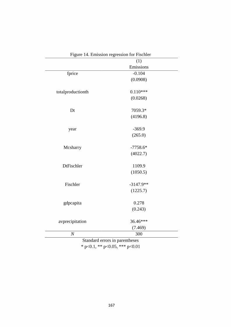
167

Figure 14. Emission regression for Fischler

(1)

Emissions

fprice -0.104

(0.0908)

totalproductionth 0.110***

(0.0268)

Dt 7059.3*

(4196.8)

year -369.9

(265.0)

Mcsharry -7758.6*

(4022.7)

DtFischler 1109.9

(1050.5)

Fischler -3147.9**

(1225.7)

gdpcapita 0.278

(0.243)

avprecipitation 36.46***

(7.469)

N 300

Standard errors in parentheses

* p<0.1, ** p<0.05, *** p<0.01

168

Robustness check.

In this final paragraph, my attempt is to verify whether production decisions

in the cereal sector are determined by intervention prices or by market

prices. In fact, part of the reasoning about the effects of the Mac Sharry and

Fischler reform is centred on the idea that cutting intervention prices and

decoupling the direct payments from the type of production, farmers would

have been encouraged to take decisions on the basis of international prices

rather than administratively set intervention prices.

In order to test this prediction, I ran the following model, where cereal

production is assumed to depend on prices and a set of controls (which

includes gdp per capita, fertilisers’ consumption and a linear time trend).

𝑌𝑖,𝑡 = 𝐵1(𝑝𝑟𝑖𝑐𝑒𝑠 ∗ 𝑁𝑜𝑛𝐸𝑈) + 𝐵2(𝑖𝑝 ∗ 𝑍𝑡 ∗ 𝐸𝑈) + 𝐵3(𝑝𝑟𝑖𝑐𝑒𝑠 ∗ 𝐷𝑡 ∗ 𝐸𝑈)

+ 𝐵4(𝑝𝑟𝑖𝑐𝑒𝑠 ∗ 𝑍𝑡 ∗ 𝐸𝑈) + 𝐵5(𝑝𝑟𝑖𝑐𝑒𝑠 ∗ 𝐵𝑡 ∗ 𝐸𝑈)

+ 𝐵6(𝑖𝑝 ∗ 𝐷𝑡 ∗ 𝐸𝑈) + 𝛿′𝑋𝑖,𝑡 + 𝛼𝑖 + 휀𝑖,𝑡 (7)

Ip are the intervention prices, 𝐷𝑡 a time dummy that goes to 1 after the

implementation of the Mac Sharry reform, 𝑍𝑡 a time dummy equal to 1 for

the years before 1993 and 𝐵𝑡 is another time dummy that goes to 1 after the

implementation of the Fischler reform. Theoretically, I expect intervention

prices to be significant before 1993 and not after, whereas international

prices should be insignificant before 1993. International prices might have

become significant either after 1993 or 2005. In fact, the direct payments

169

introduced in 1993 as a compensation for the reduction in intervention prices

were still partially coupled with the type of production. Therefore, Mac

Sharry might not have been effective in triggering a shift in production

decisions. Instead, Fischler’s reform, introducing direct payments fully

decoupled from production, should have led to production decisions fully

based on international prices. The results are provided in Figure 20 and

basically confirm the theoretical predictions. The coefficient on intervention

prices happens to be highly significant (and positive) before 1993 whereas

international prices are insignificant. Intervention prices are still significant,

even if just at the 5% level, after the implementation of the Mac Sharry

reform, suggesting that the persistent coupling between direct payments and

type of production avoided the shift towards production decisions based on

international prices. For the period before Mac Sharry we can interpret the

coefficient on ip saying that a unit increase in the intervention prices (ceteris

paribus) determines an increase in production of 118.5 thousand tons.

International prices become significant after 2005: the full decoupling of

direct payments triggers the shift of production decisions, now based on

international prices.

A word of warning has to be spent interpreting the negative coefficient on

prices; in theory, we would expect production to depend positively on prices

but, as a matter of fact, the two variables are endogenous: prices determine

production but production determines prices. A negative coefficient on

prices might be the result of a Cobweb model, where farmers take decisions

looking at past prices: if those were high, farmers would increase production

and the relative overproduction in the following period would trigger a

170

reduction in prices, explaining the estimated negative coefficient. Obviously,

this does not hold for the intervention prices that, being already known by

the farmers also for the following year, should keep the predicted (and

positive) relation with production levels.

This interpretation would be consistent with the literature that explains price

fluctuations as a phenomenon which has to be considered as endogenous to

the agricultural market (e.g., Ezekiel 1938; Day and Hanson 1991,

Finkenstadt and Kuhbier 1992, Boussard 1996, Hommes 1998, Athanasiou

et al 2008). In this literature price fluctuations in which erroneous

expectations might lead to either over or under-supply. Another interesting

extension of the cobweb model is the recent contribute of Mitra and

Boussard (2012), which analyses the effect of storage on price fluctuations,

providing a further extension of the Cobweb model.

All these recent extension of the Cobweb model refined the original,

simplistic prediction of the model first introduced by Ezekiel and overcome

some of its limitation. In particular, the idea that price fluctuation can be

recurrent, as it seems also in my empirical analysis as indicated by the

negative and significant coefficient on international prices after the Fischler

reform, has been questioned, based on the idea that if fluctuations are

recurrent, some agent in the market would recognize that this is the case and

try to take advantage of them, with the effect of eliminating this regular

fluctuation.

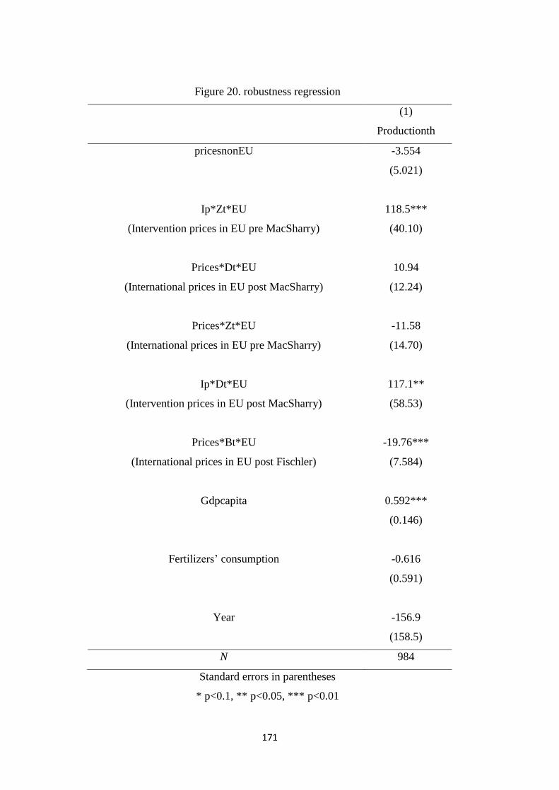
171

Figure 20. robustness regression

(1)

Productionth

pricesnonEU -3.554

(5.021)

Ip*Zt*EU 118.5***

(Intervention prices in EU pre MacSharry) (40.10)

Prices*Dt*EU 10.94

(International prices in EU post MacSharry) (12.24)

Prices*Zt*EU -11.58

(International prices in EU pre MacSharry) (14.70)

Ip*Dt*EU 117.1**

(Intervention prices in EU post MacSharry) (58.53)

Prices*Bt*EU -19.76***

(International prices in EU post Fischler) (7.584)

Gdpcapita 0.592***

(0.146)

Fertilizers’ consumption -0.616

(0.591)

Year -156.9

(158.5)

N 984

Standard errors in parentheses

* p<0.1, ** p<0.05, *** p<0.01

172

2.4 Conclusions.

This empirical research provides evidence of the positive effects of both

Mac Sharry and Fischler reforms. In particular the Mac Sharry reform was a

fundamental step in overcoming the overproduction problem in the cereal

sector and its success suggests that the reforms taken in the following years

in the remaining sectors might have had the same effect. Besides the

effectiveness of the reform in triggering a relative decrease in production, its

specific set up, substituting market support mechanism with direct payments

de-linked from the amount produced was successful in solving the budgetary

crisis that characterized the CAP in the eighties, since its origins have been

traced in the distortive incentives created by high administratively set

intervention prices. The Fischler reform seems not to have reinforced the

reduction in cereal production, leaving us with the conviction that the real

trigger of production reductions was the cut in intervention prices and the

introduction of direct payments, even if not fully decoupled. More precisely,

the results suggest that the cereal premium that cereal had in comparison

with concurrent crops during the period from Mac Sharry’s and Fischler’s

reform implementations was not big enough to trigger a sensible reduction

of cereal production when Fischler reform decoupled payments not only

from the level but also from the type of production.

The Mac sharry reform was also fundamental in reducing the amount of

GHG from agriculture and it seems that especially the set aside has been the

real determinant of the reductions. The Fischler reform determined a further

173

reduction in the emission levels but it is difficult to disentangle which

measure has been the main driver between the full decoupling of direct

payments and the introduction of the cross compliance to receive the

payments in the first place.

The test on input use, carried out as a proxy of environmental goods that are

difficult to measure as soil erosion, water pollution and so on, does not show

any evidence for both the reforms. However, the simple graph analysis in

Figure 16 shows a constant decrease in input use for the treatment group that

happens together with a substantial increase in fertilisers’ consumption in the

control group. The test on our measure of efficiency again shows no

econometric evidence, but the graph analysis suggests that the ratio between

total agricultural production and emissions has been constantly increasing in

Europe, whereas it has been stable for the other five countries analysed,

suggesting a likely positive impact of the cycle of reforms in the European

Union.

Finally, the robustness check has shown that progressively farmers’

decisions have become based on international prices, with a fundamental

role for the fully decoupled SPS introduced with the Fischler reform. This is

an important result of the present empirical analysis as it clearly shows that

intervention prices are not a driver of farmers’ production decision anymore.

It can be used to argue that Fischler’s reform has succeeded in achieving a

fully decoupling of direct payments. In fact, this robustness check is more

effective than the test on production levels to argue that the SPS introduced

by Fischler has achieved a full decoupling.

174

PART III.

PERSPECTIVES OF REFORM.

ANALYSIS OF THE UPCOMING REFORM OF THE SINGLE

PAYMENT SCHEME.

175

Introduction

With the Communication “The CAP towards 2020: Meeting the food,

natural resources and territorial challenges of the future”129

of November

2010, the Commission outlined the steps to take for a further reform of the

CAP for the post 2013. After three years of discussion and the circulation of

the official Commission legal proposals,130

a political agreement was

reached the 26th

of June 2013, outlining the core elements of the future CAP.

The guidelines of the reform regarding the main area of interest of the

present thesis (the reform of the direct payments, namely the SPS, as the

main tool affecting the cereal sector) have been stated clearly. Finally, on 16

December 2013 the Council of EU Agriculture Ministers formally adopted

the four basic regulations for the reformed CAP and the transition rules for

2014. The next step will the approval of the national options. Indeed, due to

the delays in the reform process, the new CAP will be fully operational only

from 2015. For the scope of the present thesis, the regulation of interest is

the n° 1307/2013 of 17 December 2013, which establishes the new rules for

direct payments to farmers.131

The ambition of this brief conclusion is to outline the main innovations of

the system of direct payments after 2013 and to comment on their expected

129

European Commission, “The CAP towards 2020: Meeting the food, natural resources and territorial challenges of the future”, COM 672, (2010), final 130

European Commision, “Proposal for a regulation of the European Parliament and of the Council establishing rules for direct payments to farmers under support schemes within the framework of the common agricultural policy”, COM 625 final/2, 2011 131

Regulation (EU) No 1307/2013 of 17 December 2013 establishing rules for direct payments to famrers under support schemes within the framework of the common agricultural policy and repealing Council Regulation (EC) N0 637/2008 and Council Regulation (EC) No 73/2009.

176

effects. This preliminary analysis will be based on the results of the impact

assessment conducted by the Commission and other available pieces of

quantitative and qualitative evidence.

177

Communication “The CAP towards 2020”

Commission’s Communication 672 of 2010 officially started the process of

reform of the CAP with the aim of reaching a reform for the post 2013

period. The communication was completed after an extensive public debate

that took place in the first months of 2010. The desire of the agricultural

organisations was to maintain a strong agricultural policy and the current

division in two pillars, hence keeping direct payments (pillar I) as a

substantial component of the overall policy. On the other hand, there were

consistent pressures to proceed with a more ambitious reform of the CAP

that would have possibly implied even the complete abolishment of the first

pillar with a consequent reutilisation of its funds within the second pillar.

Other important issues that were stressed were to guarantee long term food

security, food quality and, again as a main concern of farmers’

representatives, to maintain and even create new employment opportunities

in the agricultural sector.

The document stressed that the reform path undertaken at the beginning of

the nineties had contributed to the improvement of the competitiveness of

European agriculture, to create a more effective tool to sustain farm incomes

and to promote a greener agricultural policy. However a further reform is

necessary to better achieve the same goals and to correct some limitations of

the current set up. In particular, regarding the extent of the present research,

the Commission highlighted the need to analyse further the efficacy of the

SPS. Even if the Single Payment Scheme was introduced recently, the

concerns about its limits regards different aspects:

178

- the disproportion of the level of payments per hectare between farmers

both within the same country and, especially, between different countries,

with the new members currently receiving a reduced level of agricultural

payments. This has been both the result of the implementation of the

‘historical’ version of the SPS132

by the old members that still beneficiated

from payments per hectare based on the 2000-2002 reference period, but

especially regarded the situation of the countries that joined the European

Union from 2004 onwards, who were systematically allocated lower level of

payments per hectare in comparison with the old members.

- the extent to which the GAEC standards have been a sufficient

conditionality to promote a more environmental model of European

agriculture. In fact, considering that one of the main goal of the Commission

for the post 2013 CAP is the greening of the policy and that the SPS absorbs

the largest share of CAP expenditure, the fact that GAEC standards are

considered to be quite lenient in terms of environmental requirements

implies that a tightening of these standards might contribute to a

considerable greening of the policy.

- another main issue, raised by farmer organisation, is the fact that the

SPS largely beneficiates inactive farmers, which we can define in two ways:

people that use land outside agriculture and absent landowners that rent out

land for agricultural use. Regarding the first category, farmers’ organisations

132

Even for the countries (the vast majority) that opted for the adoption of the regional model with the Fischler reform it has to be said that the per hectare payments established by the Fischler reform were somehow linked to the amount that farmers used to receive under the previous set up; hence, carrying on the disproportions in direct payments typical of the “old” CAP.

179

have highlighted that the requirement of simply respecting GAEC standards

actually allow landowners that use land for other form of production besides

farming (such as trees cultivation, production of renewable energies but even

extreme cases such as airports and sport centers) to benefit from CAP

payments; that subtract funds that could otherwise be used to support

farmers’ income, which is still lagging behind non-agricultural income

regardless the improvements of the last twenty years. However, the main

complaint of farmers’ organization is that it is quite common that absent

landowners own the entitlement to receive the direct payments: hence, the

farmer that is actually cultivating the land does not benefit from direct

payments as a form of income support. The classic example is the paradox

that the largest recipient of direct payments in Europe is the Queen of

England, which actually does not need such type of income support.

In its first Communication the Commission tried to address the issue of the

reform of direct payments alongside with new proposals regarding market

measures for risk management and an enhanced rural development policy.

the Commission outlined three possible scenarios of reform for each of the

three areas. I will present the three different policy scenarios regarding the

reform of the direct payments and ignore largely the other two areas as this

is the specific area of interest of the present research.

The three policy scenarios outlined by the Commission take completely

different approaches and can be represented on a continuum between

conservation and innovation.

180

Scenario 1 was the most conservative and regarding direct payments the

only innovation would be to introduce more equity in the distribution of

direct payments between old and new member States. Besides this

modification, the system would remain the same with no greening of the

direct payments and no transfers of funds from the first to the II pillar to

increase the available funds for the financing of measures closely and

directly related to agro-environmental schemes, food quality and rural

development (no modulation scenario).

The second scenario is in the middle of the continuum and implies

redistribution of direct payments among member States (as in the first one).

However, on the top of that it would significantly change the design of direct

payments. The original intention of the Commission in the 2010

Communication was to have direct payments as actually composed by four

parts:

- a basic proportion of the existing expenditure for pillar I would be

allocated as a basic form of income support, with no conditionality attached.

- A compulsory additional aid for specific “green public goods”. That

means that every farmer will be required to implement some agri-

environmental actions with the certainty of being compensated for the

additional supplementary costs he will sustain to carry out these actions.

These measures would be compulsory and non-contractual since the aim of

the Commission is to achieve some level of provision of public good directly

from a better and more targeted use of direct payments. The idea is that since

it is difficult to proceed with a substantial modulation (transfer of funds from

the I to the II pillar to finance specific agro-environmental measures) the

181

direct greening of at least a substantial part of the I pillar might be an

alternative effective way to achieve the desired level of public goods.

- Additional payments to compensate for region specific natural

constrains and some other voluntary coupled support component for sectors

that are characteristic in some disadvantaged regions.

- A specific support for young farmers aimed at incentivising

employment in the sector.

The third scenario was based on the idea that direct payments are not an

effective way to address the overall goal of achieving a more

environmentally friendly agriculture able to provide a large amount of

environmental public goods. It is based on the phasing out of direct

payments in their current form, providing instead limited and targeted

payments for the provision of public goods and to sustain farm incomes in

regions with evident natural constrains. The third scenario clearly follows

the most radical approach for reforming the CAP and also implies the

abolishment of all market measures besides some income support systems in

case of severe crises.

It is clear that the three policy scenario define distinct and concurrent views

on how the Common Agricultural Policy should be designed after 2013. It is

also easily recognizable that the most radical approach described in scenario

three would actually trigger a drastic change of the existing policy

framework and there is no surprise that main farmers’ organisations have

repeatedly stressed the importance to maintain the current structure in two

pillars.

182

After more than one year from the publication of the Communication, the

Commission approved the legal proposals for the CAP post 2013, which I

will present in the following paragraph.

183

Legal proposals for the CAP after 2013.

A basic preliminary analysis of the legal proposals that the Commission

approved in October 2011 shows that the scenario number three, which

would imply a drastic redefinition of the CAP and in particular a phasing out

of the direct payments under the first pillar has been excluded from the set of

the available alternatives. The Commission itself in fact proposed to keep the

current division into two pillars. Given that the Commission is historically

the actor that has taken the most drastic positions regarding the reform

process, the fact that scenario number three has been already excluded with

the publication of the official proposals means that the CAP for the post

2013 will largely reflect the actual structure. In fact, it is evident that the

policy framework which emerges resemble closely the scenario number two

described above.

Regarding the structure of direct payments the new design seeks to exploit

synergies with Pillar II building on the 2003 and Health Check reforms that

decoupled payments from production and subordinating them to cross

compliance requirements regarding rural and environmental practices. With

the aim of enhancing the overall environmental performance of the CAP the

Commission has defined a set of certain practices particularly beneficial for

the environment and they will be compulsory for every farmer in order to

receive a consistent part of the direct payments. This reflects clearly the

approach of scenario number two where a compulsory aid for specific “green

public goods” was intended to be a main instrument to transform payments

under the I pillar into a measure usable to achieve also goals other than basic

income support.

184

The legal proposals clarify the share of the different instruments under the

direct payment:

- A basic payment for all farmers that will replace the actual Single

Payment Scheme. This payment, intended as a basic payment per hectare, is

meant to converge over time in order to reduce the distributional imbalances

that are the result of the Fischler’s reform calculation of direct payments,

which we should recall was linked to a reference period (2000-2002) where

the new members that joined the EU in 2004 (and in 2007) were not part of

the EU yet. That implied that with their accession to the Union, due to

budget constraints, they received proportionally less support per hectare. On

the top of that, historical imbalances were already present for old members

and the new basic payment schemes aims at reducing imbalances to a level

were the most penalised region receives at least more than 75% of the

Community average.

- A new greening component of direct payments that shall constitute up

to 30% of the annual national ceilings of the payments under the I pillar.

This means that in order to receive the full amount of direct payments the

farmers will have to fulfil specific and region specific requirements in the

following major areas: crop diversification, maintenance of permanent

pastures and safeguard of ecological focus areas.

The part that describes crop diversification specified that whether the area is

not left fallow or entirely cultivated with crops under water for a

considerable part of the year cultivation should consist of at least three crops

185

in order to benefit from the additional payment.133

Moreover, up to 5% of

farmers’ land could be converted into permanent grassland and 7% of the

eligible hectares, besides the area allocated to permanent grassland, should

constitute ecological focus area such as buffer strips, land left fallow,

terraces, landscape features or afforested areas.

What is clear is that in order to benefit from the additional greening

component of the direct payments the farmers will be required to fulfil some

minimum requirements in terms of crop rotation and definition of ecological

focus areas. This shows clearly how the Commission attempts to transfer

into the I pillar a set of instrument that would have normally been under the

second pillar and in particular under the axis 2 of the II pillar, which regards

the agro-environmental schemes.

One of the goals of this final part is to comment on this political choice,

establishing whether this inclusion of these instruments under the I pillar can

be effective for the overall goal of achieving higher provision of public

goods. On the other hand it has been claimed that this choice reveals instead

the lack of political agreement on a more ambitious reform that would have

drastically changed the set-up of the CAP or at least implied a high

modulation/transfer of resources from the I to the II pillar.

- Up to 5% of annual national ceilings for direct payments could be

allocated to farmers in areas facing specific natural constrains. This means

that each country can decide to sustain producers on marginal land directly

133

Mentioning the possibility for the land to be left fallow will be important when I come to the analysis of the political agreement on the future reform.

186

using funds from the I pillar with the predictable effect that the amount

dedicated to this particular objective might increase.134

- Up to 2% of annual national ceilings can be allocated to support the

activities of young farmers.

After almost two years since the approval of the legal proposal, the

European Parliament, the EU council of Ministers and the European

Commission have reached an agreement on reforming the common

agricultural policy post 2013. Commisioner Dacian Ciolos is convinced the

agreement will lead to far-reaching changes: making direct payments fairer

and environmentally focused, improving the competitiveness of European

agriculture and strengthening the position of farmers within the food

production chain.

134

This element, together with the greening of a substantial amount of the funds under the I pillar has been criticised as a measure that might interfere with the goal of achieving a full decoupling. In fact, in my conclusions I will show how there is substantially a trade-off between achieving a full decoupling and using particular instruments to achieve a set of other goals such as income support and provision of environmental goods.

187

The Political agreement on new direction for the common agricultural

policy and the regulation 1307/2013 of 17 December 2013 on the future of

direct payments.

The political agreement clarified that the aim of making the CAP fairer

implies the elimination of every historical reference in the mechanism used

to compute the amount of direct payments. As is has been shown also the

SPS system was largely based on reference periods prior to the access of the

ten new East European member in 2004 (and Romania and Bulgaria in 2007)

determining substantial imbalances in per hectare payments among States.

“Convergence” is an important objective of the reform and the agreement

confirms the orientation already expressed in the legal proposals regarding

the need to ensure that no single member State receives less than 75% of the

Community average by 2019. Moreover, the agreement clarifies the

convergence rules within countries and regions: in particular differences in

the levels of per hectare payments will be reduced assuring that aid will not

be less than 60% of the average per hectare aid allocated in a single

administrative area. The political agreement clarifies that only active farmers

will benefit from income support schemes.

Regarding the greening of the I pillar, the political agreement confirms the

orientation of the legal proposals, stressing that 30% of direct payments will

be linked to three environmentally-friendly farming practices: crop

diversification, maintaining permanent grassland and conserving 5%, and

later 7%, of areas of ecological interest as from 2018 or measures considered

to have at least equivalent environmental benefits.

188

Finally, the regulation n° 1307/2013 largely confirms the outcomes of the

legal proposals and clarifies better issues such as convergence, the capping

of direct payments for the bigger beneficiaries and the controversial issue of

the “active farmers”. The regulation also confirms the greening of the first

pillar, which I will analyse in more detail in the next paragraphs.

As for the active farmers issue, it has been raised continuously by farmer

organisation throughout the negotiations as one of the worst distortions of

the previous policy framework. In this sense, the regulation shed light on the

definition of active farmer, which is specified in article n° 4(2):

“ (a) “farmer” means a natural or legal person, or a group of natural or legal

persons.. .. whose holding is situated within the territorial scope of the

Treaties, as defined in Article 52 TUE in conjunction with articles 349 and

355 TFEU, and who exercises an agricultural activity”.

Moreover, the same article defines agricultural activity as follows:

“agricultural activities” defined as follows:

“Production, rearing or growing of agricultural products, including

harvesting, milking, breeding animals, and keeping animals for farming

purposes.

Maintaining an agricultural area in a state which makes it suitable for

grazing or cultivation without preparatory action going beyond usual

agricultural methods and machineries, based on criteria established by

Member States on the basis of a framework established by the Commission,

or

Carrying out a minimum activity, defined by Member States, on agricultural

areas naturally kept in a state suitable for grazing or cultivation.”

189

Moreover, article 9 on “active farmers” also specifies that no payments

should be corresponded to persons for which the amount of the direct

payments would be lower than 5% of their income from non-agricultural

activities. This additional measure is indeed aimed at excluding from the

beneficiaries part time farmers that cannot claim to live off agriculture.

Coming to the convergence, it is regulated by article n°25 of the new

regulation, that establishes: “Member States shall provide that, at the latest

for claim year 2019, no payment entitlement shall have a unit value lower

than 60 % of the national or regional unit value in 2019”, again, confirming

the orientation already emerged in the legal proposals.

A final mention is dedicated to the “capping” of direct payments, which is

regulated by article n° 11 that states that “ Member States shall reduce the

amount of direct payments to be granted to a farmer pursuant Chapter 1 of

Title III for a given calendar by at least 5% for the part exceeding EUR

150000”.

It is clear that with the capping of direct payment and, especially, with a

better definition of the “active farmer”, the Commission has responded to the

pressures of the farming organisations that have historically complained

about the distortions in the repartition of direct payments. The capping is

clearly aimed at reducing the overall level of support to bigger farmers, who

are clearly big enough to survive with a lower level of subsidy, whereas the

redefinition of the active farmer, even if somehow problematic especially

regarding the criteria “Direct Paymet > 5% non- agricultural income” is at

190

least useful at excluding from the beneficiaries persons and legal persons

that do not carry out any type of agricultural practice.

191

Preliminary analysis of the effectiveness of the proposed CAP reform

Given the very recent agreement on the future of the CAP post 2013 it is

difficult to provide something more than a preliminary analysis of the likely

effects of the reform. In the present research I will rely mainly on the impact

assessment (2011)135

carried out by the Commission after the approval of the

legal proposals and on some independent studies, among which the work of

Tangerman (2011)136

stands out for the rigour of the analysis and for the

independent and heterodox views expressed, especially regarding the

analysis of the “greening” of direct payments. Another source of information

is the OECD report “Disaggregated impacts of CAP reforms” (2011)137

which provides quantitative and qualitative evidence on the effects of the

2003 and Helath Check reforms but can be used to comment on the effects

of the reform of the direct payments. Lastly, De Filippis et all (2012)138

have

produced an organic review of the new CAP set up and their contribution is

essential to understand the economic impact of the reform on farmers’

welfare, which is crucial in the present analysis.

Considering that the aim of my research has been to prove whether

successive reforms of the CAP has led to a more competitive agricultural

sector (with payments completely decoupled from the level and the type of

production) and whether they have helped reducing the environmental

135

European Commission “Impact assessment. Common Agricultural Policy toward 2020”, SEC 1153 (2011) final. 136

S. Tangermann, “Direct payments in the CAP post 2013”, Directorate General for Internal Policies. Policy Department B: structural and cohesion policies, European Parliament, 2011. 137

OECD “Disaggregated impacts of CAP reforms”, OECD publications, Paris, 2011. 138

De Filippis et all., “La Nuova PAC 2014-2020: un’analisi delle proposte della Commissione”, edizioni Tellus, Roma, 2012.

192

impact of the policy, I will limit my considerations on how the reform of the

direct payments might impact on those two main objectives. Before that I

will comment on the likely effects on income; in fact, this has been one of

the major objective of the CAP from its birth, the challenge being, now,

sustaining incomes without the distortions that characterized the policy

before Mac Sharry and that still partially affected it before the

implementation of progressive forms of decoupling.

Effects on income.

The claim of the impact assessment carried out by the Commission in 2011

as regards the so-called “integration scenario” (scenario number two above)

is that the direct payments will better achieve the goal of providing a stable

income and will lead to a more balanced allocation of direct payments

between members and farmers within the same country. On the top of that,

the greening component is predicted to be particularly beneficial for certain

basic environmental public goods.

However, regarding the effects of greening of farm income and profitability

the report highlights the importance of getting a right balance between the

additional costs that the “green” measure will impose to farmers and the

amount of payments per hectare that will be allocated to the virtuous

farmers, which we have seen can go up to the 30% of the national ceiling of

the first pillar. In fact, green policies might affect farm revenues in at least

three ways: by increasing costs of production, by diminishing level of

production and revenue and by impeding the shift to a more profitable

193

(intensive) production system. The two costs are easily measurable

providing data availability (even if they would vary considerably from

region to region) whereas the third one is an opportunity cost that would be

more difficult to quantify and that would depend even more on location-

specific elements. The report estimates that the resulting average cost per

hectare of all the greening measures together across the EU 27 would vary in

a range from 33 to 41€ per hectare, even if the variation is considerable. As

an example, the costs per hectare will be lower for marginal regions where

extensive farming was already taking place before the reform whereas for

area of intensive and one-crop farming (monocultures) the cost will be

dramatically high. The estimates are that on average the “greening option”

will result in a decrease in the average income ranging from -3,2% and -

1,4%. However, the same report notes as positive variations of farm income

might actually occur for farmers that are already respecting stricter

environmental requirements and how these might be a benefit or marginal

farmers. Regarding these productions the greening of a considerable part of

the first pillar will reinforce phenomenon already highlighted by Chatelier

and Guymard (2011)139

in their paper on the distributional effects of the

Health check in France. The simulations on farm incomes, conducted with

the Farm Accountancy Data Network (FADN), demonstrate a shift of direct

payments in favour of extensive grazing farms, mainly those with a high

proportion of pasture in their rotation. By contrast, crop farms and farms

with intensive production of cattle are losers. This demonstrates how moving

towards a flatter rate has also production and environmental consequences.

139

Chatelier and Guymar (2011), in OECD “Disaggregated impacts of CAP reforms”, OECD publications, Paris, 2011.

194

This feature regarding distributional effects of a flatter rate is also quite

straightforward and follows from the fact that also the SPS payments were

based on a reference scenario based on Mac Sharry payments that largely

favoured intensive farming systems and arable crops.

The last element of the reform that will have an impact on the income of

farmers is the application of the convergence criteria. As De Filippis et all.

(2012) highlight, the application of the “convergence criteria” will have

different effects in different countries and also depending on the type of

cultivation. The authors highlight that Italy in particular will be penalised by

this declination of the convergence criteria and advocate an ad hoc measure

to counteract this negative effect on Italian farmers. As for Italy, the authors

stress that the national ceiling would decrease from 4024 mld of Euros in

2014 to 3842 in 2019 claiming that Italy alone would contribute to almost a

third of the funds “moved” by the convergence mechanism. As a percentage

reduction of previous payments, only Holland, Belgium and Malta would be

more penalised than Italy, whereas France and Germany would lose only

marginally, UK would experience a slight increase between pre and post

reform payments and, as expected, the countries that will benefit the most

are the new members (but also Spain and Portugal).

In particular, the reason why Italy will be particularly penalised lies in the

fact that it had adopted the historical model for the direct payments with the

Fischler reform. Given that the convergence relates to the “average payment

per hectare” obtained dividing the national ceiling by the surface eligible for

direct payments as for the year 2009. This is exactly the origin of the

penalisation as in 2009 the countries that adopted the regional model

195

extended the eligible area to all the agricultural area, regardless of the

cultivation whereas that measure remained the same for the countries

adopting the historical model. As a consequence of that, when dividing the

national ceiling for the admissible area the average payment per hectare for

Italy results in a considerably greater number, which is the base one which

the convergence criteria is applied. To clarify the matter, the following table

from De Filippis (2012) gives an intuitive and graphic representation of the

predicted effects in terms of redistribution of direct payments among

different member states. Quite clearly the redistribution will lead to a

compensation for the countries that historically experienced lower levels of

payments but that is done penalising the countries that opted for the

historical method to implement the Fischler reform.

196

To conclude, their effect on farm income will probably depend on the type

of farming considered. The greening of the direct payments will add to the

increasing convergence in the sense that both measure will tend to favour

more extensive farming systems which are likely to involve marginal

farmers while penalising intensive farming in comparison with the pre

reform scenario.

However, the impact assessment states clearly that overall there will be a

reduction in the average income. This prediction is shared by Tangermann

(2011) that states that depending on the share of direct payments dedicated

to the “greening” component the negative effect on overall farm income

might become considerable. In fact, considering that they will likely subtract

resources from the basic direct payments and that they will impose extra

costs on the farmers, it is straightforward that the overall effect is that the

new direct payments will generate less farm income, per Euro spent, than the

SPS scheme. This is a logic consequence of the additional costs implied by

the “green” measures in pillar I. The fact that this requirements affect such a

generalised instrument and therefore every farm eligible for direct payments

is also another issue. In fact, as it will be clear when analysing the effects of

the reform on the provision of public goods, the generalisation of higher

environmental standards might create considerable costs (in terms of loss of

revenue and opportunity costs) to the intensive farming systems while it is

not clear if they are the most efficient way to increase the provision of public

goods.

Another measure included in the reform aimed at improving farmers’

income is the focus on active farmers, however, I will briefly discuss it in the

197

next paragraph as I belief that the actual (positive) effects on agricultural

incomes are bound to be limited whereas the measure raises concerns about

a very important aspect of the CAP: its capacity to provide a form of support

completely decoupled from production in order to increase the

competitiveness of the overall agricultural sector and to comply with the

international regulation under the WTO agreement for agricultural markets.

198

Effects on agricultural competitiveness and Green box compatibility.

One main question that, I believe, has not been addressed properly in the

recent debate on CAP reform is whether the new direct payment system will

maintain, enhance or diminish the level of decoupling achieved with the

Fischler reform. This concern has to be raised considering two features of

the upcoming reform: the attention on active farmers and the measures that

are required in order to benefit from the green component of direct

payments.

As Swinbank and Tranter (2005)140

pointed out already for the SPS scheme,

payments are totally decoupled whether they are completely independent

from the fact that production is even taking place. The question they raised

about the SPS is that even if the amount of payments received did not

depend neither on the level nor on the type of production, the GAEC

standards and in particular the requirement to keep the land in good

agricultural conditions might actually be partly correlated with production.

The reasoning is the following: differently from a totally decoupled payment

system, the fact that the owner of an hypothetical unit of marginal land

would still have to do some work on it in order to benefit from the payments

might end up creating the incentive for him either to produce something on it

or to convert it into grassland (which would boost livestock production) or to

rent it out. In other words, the fact that something has to be done in order to

140

Swinbank, A., and R. Tranter (2005), Decoupling EU Farm Support: Does the New Single Payment Scheme Fit within the Green Box? The Estey Centre Journal of International Law and Trade Policy, Vol. 6, pp. 47-61.

199

benefit from the payments creates the incentive either to allocate more time

to on farm activities or to rent the land to some other producer and benefiting

from the SPS payments. Going back to the literature review, this argument

follows the Ahearn, M., El-Osta, H. and Dewbre (2006) paper on the effects

of direct payments on labour allocation: direct payments (and especially

payments which imply measures such as the ones under the new “green”

component) can distort labour allocation and increase the likelihood that

farmers that would have left production stay active.

Coming to the “greening” of the direct payments, the argument would work

in the same way and actually become more compelling. An example might

help clarifying the problem. Consider the owner of a unit of marginal land.

In a fully decoupled scenario aimed at sustaining temporarily farm incomes

in order to regulate the farm exodus, he would receive direct payments for a

limited period of time (ten years in the bond scheme proposed by Swinbank

and Tranter in their most famous contribution)141

so that only the really

competitive farmers would remain in production in the long run. That was,

by the way, the initial goal when direct payments were initially introduced

before becoming somewhat a permanent feature of the CAP. This

hypothetical farm would have to figure out whether he could compete in the

market space, knowing in advance that he would benefit from direct

payments for a limited period of time. If yes he would have a temporary help

to increase economy of scales and improve competitiveness. If not he would

have time to develop some extra-agricultural activity with the positive result

of having a safety net against unemployment. Now, abstracting and

141

Swinbank, A., and R. Tranter (eds.) (2004), A Bond Scheme for Common Agricultural Policy Reform. Wallingford: CABI Publishing.

200

generalizing, a fully decoupled payment scheme would favour the self-

selection of efficient farmers with the long run result that only really

competitive farmers would keep producing. The effect on total production is

clear in the sense of a reduction in comparison with the pre-reform scenario,

for example in comparison with a system based on some form of price

support.

In a system were direct payments are corresponded depending on some

measures that imply on-farm activities, instead, the effect could be an

incentive to allocate even more time to those activities or anyway to rent out

the land in order to benefit from the payments; maybe to another producer

with sufficiently big economies of scale to make cultivation of that marginal

land profitable. The overall effect would be in any case a boost in total

agricultural production in comparison with the bond scheme/free market

scenario.

This argument is raised by Tangermann, who stresses the results of

Swinbank and Tranter’s research and add that this distortive effect of direct

payments is particularly critical especially considering the fact that the

payments will be corresponded only to active farmers. The author stresses

that the “greening” component of the new direct payments might be

problematic in “Green box” term as they will probably undermine the

decoupled nature of direct payments overall. Regarding the “active farmers”

focus of the new direct payments, it has been introduced to guarantee that

the payments would actually sustain farmers’ income and not the one of

absent landowners, the aim being supporting farm income since it is lagging

behind non-agricultural income. However, Tangermann highlights how this

201

requirement might be meaningless in practice due to the fact that, even if the

payments were corresponded to the farmers that rent out the land from the

landowner, the latter will probably be able to extract the correspondent

amount as a rent premium. In other words, direct payments are going to be

captured in rents anyway and the re-focusing of direct payments on active

farmers only will not be an effective way to guarantee the subsidy ends up to

the actual producer and not to unproductive landlords.

This standard prediction of neoclassical models has been recently challenged

by empirical researches which have shown that, at least considering the

empirical evidence examined, landlords are not able to capture all subsidies

in rents but just a minor part (Kirwan, 2009)142

. However, the theoretical

explanation of the phenomenon might be location specific and apply to

places (such as the US) where land is not a scarce resource and therefore the

bargaining power of the farmer is enhanced relative to the landlords’. To

conclude this brief parenthesis, the extent to which the focus on active

farmers will be effective in boosting agricultural income is then a matter of

empirical testing also for an agricultural sector as the European one it is

likely that the neoclassical prediction might prevail.

The very important element though is that this focus on active farmers might

act alongside the effects of the greening in the sense of reducing the

decoupling nature of direct payments, hence making them more difficult to

justify and include under the “Green box” in the WTO agreements on

agriculture. The reason why this focus might alter the decoupling nature of

142

Barrett E. Kirwan, “The Incidence of U.S. Agricultural Subsidies on Farmland Rental Rates” Journal of Political Economy, Vol. 117, No. 1 (February 2009), pp. 138-164.

202

the new direct payments in fact is rather obvious and that is definitely an

issue that might impact on the goal of improving the competitiveness of

European agriculture. The two measures together are therefore likely to

trigger a positive effect on production in comparison with a fully liberalised

scenario or with a total decoupling one; they would probably help keeping in

production farmer’s that would have had to leave the sector otherwise.

Having stated some plausible reasons to be somehow sceptical about two of

the main aspects of the reform of the direct payments, it has to be said that

there is also a valid justification of such sort of measures, in particular the

claim that they are necessary to incentive the provision of public goods. As

the literature about market failures stresses, a pure market based set of

incentives is often unable to pursue public interest. Agriculture itself can

produce valuable environmental public goods or create environmental losses

whose burden falls on society overall. The issue here is to determine whether

the value of the public goods created outweigh the cost of the measures put

in place to achieve them; not only the economic cost of the policy itself but

the private losses the farmers have to sustain and the opportunity costs as

well. Briefly, it is important to determine whether the policy are Pareto

improvements or not. In order to do that rigorously we should be able to

carry out a detailed cost benefit analysis including precise estimates of the

costs and the benefits foreseen. Being that almost impossible as it implies

issues such as the monetary valuation of public goods, a realistic approach

would aim at verifying two facts: are the policies implemented effective in

order to reach the goals? The second question, instead, regards efficiency:

are the instruments proposed able to achieve the proposed goals in the most

203

efficient way? Could we achieve the same results doing something else and

maximizing total Welfare? The last paragraph aims at providing a

provisional answer to this question.

Finally, also the increased focus on sustaining active farmers income has valid

reasons if we consider that before the reform, payments were allocated even to

people absolutely not involved in agricultural activities. In this sense, the

recent regulation of December 2013 contributes to the solution of the problem

specifying the two criteria for the definition of active farmers already

mentioned above.

Besides the limits of this approach, an immediate and positive result will be to

exclude from the beneficiaries legal persons that have not got anything to do

with agricultural production, correcting the distortions of the previous policy

set up, under which it was possible that legal persons such as sport centres and

even airport could still claim agricultural payments if their land had

previously been used for agriculture. De Filippis et all. (2012) highlight how

the “DP > 5%” criteria is more debatable but anyway agree that this correction

would allow for more funds to be redistributed between actual farmers, which

should be the logical scope of an agricultural policy.

204

Effects of provision of public goods.

Coming to the analysis of the expected effects on the capacity of the

European agriculture to provide public goods, the impact assessment carried

out by the Commission stresses that the inclusion under the first pillar of

measures directly aimed at providing public goods will enable the

agricultural sector to provide a generalised set of public goods which were

not delivered by the previous cross compliance requirements. The claim is

that the subordination of a significant proportion of direct payments to

relatively high standards will act as a sort of “super cross compliance” that

would force every farmer to satisfy higher environmental standards, with the

expectation that this type of approach would help delivering more public

goods.

The work of Tangermann is particularly instructive and I will largely reflect

his approach, stating from the very beginning that I do not agree with its

criticism regarding the political implications of the policy.

In particular, Tangermann states that the inclusion of measures such as crop

rotation, pasture maintenance and the safeguard of ecological focus area

under a generalised instrument such as the direct payments of the first pillar

might be an effective way to achieve a certain level of public gods but it is

definitely not the most efficient policy. In fact, environmental public goods

can have differing geographical dimensions, from global ones such as the

reduction of GHG emissions and of air pollution, to local ones such as flood

and fire prevention or the maintenance of valuable agricultural landscapes.

205

Given this multidimensional nature of the concept of environmental public

goods, the critique is that such a generalised instrument might be inefficient

in the sense that a more sector and local specific approach might address

better the problem, achieving better overall results with a reduced amount of

resources. Moreover, given the fact that many environmental public goods

are of a primarily local nature, it follows logically that following a

standardized approach throughout the entire European Union cannot be the

best strategy to address the huge variety of local needs. The reasoning is

pretty straightforward; for example setting of relatively high environmental

standards for intensive farming can create massive private losses in terms of

revenue losses and opportunity costs, whereas the benefits from the respect

of such standards might be negligible, especially considering that the same

resources might be used to promote particular actions (for example the

safeguard of biodiversity or instruments to improve water quality or flood

prevention) on marginal land that would create more valuable public goods

and would not be a cost for the producers since the revenue losses and the

opportunity costs. To sum up, even though the provision of public goods of

EU wide importance should be pursued at an European level, the fact that

such specific measures are included under a very general instrument will

decrease the efficiency of the policy.

However, my position differs from Tangermann regarding the political

interpretation of the reform. The author states that if the aim of the reform is

to shift the “dividing line” between the two pillars in order to make pillar

one a concurrent tool to achieve goals that have been traditionally kept under

pillar two is not a practical idea and it is likely to create a lot of technical

206

difficulties. He brings the example that compensating farmers for the actual

costs sustained to carry out a particular policy is such an individually based

action that should be carried out under the contractual agreements typical of

the II pillar and cannot be extended to the I pillar since those payments are

generalized. Another matter of concern is the fact that the I pillar payments

are completely funded by the European Union and the inclusion of measures

that used to be co-financed under the II pillar might decrease State

accountability and possibly affect the implementation of the measures.

Even though the concerns expressed by Tangermann are largely

understandable, I would tend to see the shift of some measures under the

first pillar from a different perspective; in particular, I believe we should

approach the reform considering the three scenarios that were outlined from

the very beginning and the risk that the consultative process started three

years ago might have ended substantially with no reform of the CAP. In this

light, the greening of the first pillar can be interpreted as a sort of

compromise between the view of those who wanted to keep the CAP as it

was and the advocates of a revolutionary reform. Given the overall goal of

improving the public good provision from the agricultural sector and the

difficulties to reach a reform based on a decisive shift of resources from the I

pillar to the II one, transferring the measures under the first one, inverting

the logic, is certainly inefficient but possibly the better compromise possible.

In fact, the opposition of farmers’ organisation to a reform based on the

scenario number three are largely known. Even the member States were

against a drastic change as it would have implied an increase in their

budgetary burden. In other words, if the goal of the Commission was to

207

change the priorities of the agricultural policy stressing its environmental

implications, the choice of transferring measures from the second to the first

pillar instead of funds from the pillar I to pillar II might have been the only

politically acceptable compromise given the positions of the relevant actors

and the risk of having no reform at all.

208

Conclusions.

This thesis analyses the successive reforms of the CAP from the early

nineties. After defining the context that lead to the reform, the second part

carries out an in deep empirical analysis and my results largely confirm the

ones of the existing literature. First, Mac Sharry reform has had a significant

impact on production, proving that even a system just partially decoupled

(from the level but not from the type of production) was effective in

tempering the distortionary effects of the price support system.

In my analysis, Fischler reform seems not to have had significant effects in

terms of decrease in production.143

Moreover, the robustness check on prices

demonstrates that international prices became significant in explaining

production decisions just after the Fischler reform, validating the claim that

these payments were really decoupled and lead to market based decision

making. The test on the effects of the two reforms on GHG emissions is

robust and significant, confirming the expectations that a progressive

decoupling of direct payments would have helped the delivery of global

public goods such as greenhouse gas reductions. These results are in line

with the existing literature and with the theoretical expectations derived from

economic theory and contribute to the literature on the effects of the CAP

reform process.

Coming to the final chapter, I tried to present some features of the reform

that has been debated in the last three years, concluded with the sign political

agreement of the 26th

of June 2013. I outlined the main contents of the

143

In the second part I also addressed this issue clarifying how the set-up of my test might be itself a potential explanation for this partially unexpected result.

209

reform and carried out a preliminary analysis. My conclusions regarding

three major areas are the following:

- The effects on income are bound to be negative overall. Making costly

agro-environmental measure compulsory will determine significant

loss of revenues and opportunity costs for the producers, alongside

with the considerable costs of the policy for the European budget.

Another basic result is that the higher level of convergence will favour

the income of the marginal farmer and penalise intensive farming in

comparison with the past SPS scheme.

- Probably the major concerns are related to the fact that the reform

might diminish the competitiveness of European agriculture due to its

attention to “active farmers” and the inclusion of some “green”

measures under the first pillar. The reasoning is developed in the third

part and claims that this two innovations might create a partial

recoupling of the policy even if it would be a sort of “green”

recoupling, therefore probably more legitimate. Another concern is

whether the reformed direct payments will comply to the “Green box”

under the WTO agreement.

- The effects on the provision of public good are certainly positive. The

inclusion of agro-environmentally related measures under the first

pillar is bound to increase the amount of public goods delivered by

European agriculture. I have also argued, following Tangermann’s

contribution, that this will not be done in the most efficient way.

However, my overall judgment of the reform is less critic than the one

provided by the author. Considering the political context and the risk

210

of having no reform, given the initial goal to enhance the “greening”

of the CAP I believe that the solution found is a good compromise and

a quite clever way to get around the predictable opposition to any sort

of more radical reform that would have question the general structure

of the CAP as we know it.

211

Bibliography

R. Ackrill, “The Common Agricultural Policy”, UACES, Sheffield

Academic Press, 2000.

Autor, D. (2003) “Outsourcing at will: the contribution of unjust dismissal

doctrine to the growth of employment outsourcing”, Journal of Labour

Economics, vol. 21, no. 1, pp. 1-42.

Bakhshy, R. S. Gray ‘Acreage response to whole farm income stabilisation

programs’ Journal of Agricultural Economics, Vol. 63, No. 2, 2012, 385–

407

D. Baldock (1990) “Agricultural and habitat loss in Europe”, World Wild

Fund for Nature, London, 1990.

R. Baldwin and C. Wiplosz, (2003) “The Economics of European

Integration”, Mac Graw-Hill, 3rd

edit.

Barrett E. Kirwan, “The Incidence of U.S. Agricultural Subsidies on

Farmland Rental Rates” Journal of Political Economy, Vol. 117, No. 1

(February 2009), pp. 138-164

Beard, N., Swinbank,A. “Decoupled payments to facilitate CAP reform”,

Food Policy 26 (2001).

J.M. Boussard (1996) “When risk generates chaos”, Journal of Economic

Behavior & Organization, Volume 29, Issue 3, May 1996, Pages 433–446

William A. Brock, Cars H. Hommes, (1998) “Heterogeneous beliefs and

routes to chaos in a simple asset pricing model”, Journal of Economic

212

Dynamics and Control, Volume 22, Issues 8–9, 3 July 1998, Pages 1235–

1274

Francesca Bignami (2007), Associazione Alessandro Bortola, collezione

tesi on-line, n°18, Luglio 2007.

Bignall E., and McCracken D., (1996)” The Ecological Resources of

European Farmland” in Whitby M.C., “The European Environment and the

CAP Reform: Policies and prospects for conservation” CAB International,

Wallingford.

Chatelier and Guymar (2011), in OECD “Disaggregated impacts of CAP

reforms”, OECD publications, Paris, 2011.

Commission of the European Communities (1958), “First General Report

on the Activities of the Community, Brussels.

Commission of the European Communities (1958a), “Recuil des documents

de la conference agricole des etats members de la communaute economique

europeenne a Stresa au 12 Juillet 1958 ", Brussels.

Commission of the European Communities, “Perspectives for the Common

Agricultural Policy”, COM (85) 33 final, Brussels, 15 July 1985.

Commission of the European Communities, “The development and future of

the CAP”, COM (91) 100, final, 1 February 1991.

W. Cochrane, (1958) “Farm prices: myths and reality”, Minnesota

University Press.

Cunha and A. Swinbank, (2012) “An inside view of the CAP reform

process”, Oxford University Press.

De Filippis et all., “La Nuova PAC 2014-2020: un’analisi delle proposte

della Commissione”, edizioni Tellus, Roma, 2012.

213

European Commission, “The CAP towards 2020: Meeting the food, natural

resources and territorial challenges of the future”, COM 672, (2010), final.

European Commission, “Proposal for a regulation of the European

Parliament and of the Council establishing rules for direct payments to

farmers under support schemes within the framework of the common

agricultural policy”, COM 625 final/2, 2011

H. De Gorter and K.D. Meilke “Efficiency of Alternative policies for the

EC’s Common Agricultural Policy”, American Journal of Agricultural

Economics, August 1989.

De Gorter, H., Nielson, D.J., and Rausser, G.C. (1992) “Productive and

Predatory public policies: research expenditures and producer subsidies in

agriculture”, in “American Journal of Agricultural Economics”, n°74, pag

27 – 37.

European Commission, 1985. “Perspectives for the common agricultural

policy. Communication of the Commission to the Council and the

Parliament”.

European Commission (1994) “EC Agricultural Policy for the 21st

Century”.

European Commission “Impact assessment. Common Agricultural Policy

toward 2020”, SEC 1153 (2011) final.

M. Ezekiel (1938) “The Cobweb theorem” The Quarterly Journal of

Economics

Vol. 52, No. 2 (Feb., 1938), pp. 255-280

214

A. Fearne, “The History and Development of the CAP 1945-1990”, in C.

Ritson and D.R. Harvey, “The Common Agricultural Policy”, 1997, CAB

international, Wallingford, UK.

B. Finkenstädt, P. Kuhbier (1992), “Chaotic dynamics in agricultural

markets”, Annals of Operations Research 1992, Volume 37, Issue 1, pp 73-

96.

Lilyan E. Fulginiti and Richard K. Perrin “Prices and productivity in

Agriculture”, in The Review of Economics and Statistics, Vol. 75, No. 3

(Aug., 1993), pp. 471-482.

J. Gale Johnson, "Comparability of Labor Capacities of Farm and Nonfarm

Labor," American Economic Review, June 1953, 43(3), pp. 296-313,

J. Gale Johnson, " An Appraisal of the Data for Farm Families," in An

appraisal of the 1950 census income data. NBER studies in Income and

Wealth, Vol. 23, Princeton: Princeton U. Press, 1958a, pp. 287- 301.

B. L. Gardner, (1992), “Changing economic perspective on the farm

problem”, in “Journal of Economic Literature”, Vol. XXX (March 1992),

pp. 62-101

Goodwin, B. K. and A. K. Mishra. ‘Are “Decoupled” Farm Payments

Really Decoupled? An Empirical Evaluation’. American Journal of

Agricultural Economics Vol. 88(1), 2006: 73–89.

Gohin, A., ‘Assessing CAP reform: Sensitivity of Modelling decoupled

policies’. Journal of Agricultural Economics, Vol. 57 No. 3, 2006, 415-

440.

W. Grant, “The Common Agricultural Policy”, 1997, The European Union

Series, Palgrave MacMillan.

215

Hathaway, D. E. (1964) “Problems of progress in the agricultural

economy”. Glenview, IL: Scott, Foresman,

A. Hearn, M., El-Osta, H. and Dewbre, J. ‘The impact of coupled and

decoupled government subsidies on off-farm labor participation of U.S.

farm operators’, American Journal of Agricultural Economics, Vol. 88,

(2006) pp. 393–408

Hennessy, D. A. 1998. The Production Effects of Agricultural Income

Support Policies under Uncertainty. American Journal of Agricultural

Economics 80(1): 46–57.

IEEP (2008), “The Environmental Benefits of Set-Aside in the EU: a

summary of evidence”, Prepared by The Institute for European

Environmental Policy for Department for the Environment, Food and Rural

Affairs , February 2008.

Jenkins, T. (1990), “Future harvester: the economics of Farming and the

Environment”, Council for the protection of rural England, London

T. Josling “A formal approach to Agricultural Policy” in “Journal of

Agricultural Economics”, Volume 20, Issue 2, pages 175–196, May 1969.

Nicholas G. Kalaitzandonakes “Price Protection and Productivity Growth”

American Journal of Agricultural Economics. n° 76 (November 1994):

722-732

Kean and Lucey (1997) “The CAP and the Farmer” in Harvey, “The

Common Agricultural Policy”, 1997.

Key, N., R. N. Lubowski and M. J. Roberts, ‘Farm-level production effects

from participation in government commodity programs: did the 1996 federal

216

agricultural improvement and reform act make a difference?’ American

Journal of Agricultural Economics, Vol. 87, (2005) pp. 1211-1219.

M. Lanfranchi “Dal Trattato di Roma all’Health Check: mezzo secolo di

storia di politica Agricola comunitaria”. Edizioni Dr. Antonino Sfameni,

Messina, 2008.

Legg, W. (2002) “The evolution of agricultural policies in OECD countries

as reflected by the level and structure of agricultural support” in “China in

the Global Economy Agricultural Policies in China after WTO Accession”,

OECD.

L. Lindberg, 1963, “The Political Dynamics of European Economic

Integration”, Oxford University Press, Oxford, 261 – 283.

Lockwood, B. And Porcelli, F. (2012) "Incentive Schemes for Local

Government: Theory and Evidence from Comprehensive Performance

Assessment in England", American Economic Journal: Economic Policy,

vol. 5, n°3, August 2013.

S. Masholt “The future shape of agricultural policy”, European

Communities, Joint Information Service. Newsletter on the Common

Agricultural Policy, N°1, January 1968.

S. Mitra, J.M: Boussard (2012), “A simple model of endogenous

agricultural commodity price fluctuations with storage”, Agricultural

Economics, Volume 43, Issue 1, pages 1–15, January 2012

OECD (1994) “Farm Employment and Economic adjustment in OECD

countries”, OECD Publishing, Paris.

OECD (2011) “Evaluation of Agricultural Policy Reforms in the European

Union”, OECD Publishing, Paris.

217

OECD “Disaggregated impacts of CAP reforms”, OECD publications,

Paris, 2011.

OEEC (1957), “Agricultural Policies in Europe and North America: Second

Report of the Ministerial Commitee for Agriculture and Food”, Paris, 2007.

Kevin H. O’ Rourke “The European grain invasion”, in The Journal of

Economic History, Vol. 57, No. 4 (Dec., 1997), pp. 775-801, Cambridge

University press.

Neville-Rolfe, 1984, “The Politics of Agriculture in the European

Community”, London, Policy Studies Institute.

Potter, C. (1996), “Decoupling by degrees? Agricultural Liberalisation and

its Implication for Nature Conservation in Britain”, English Nature

Research Reports no. 196, Peterborough.

Potter, C. and Goodwin, P. (1998),“Agricultural liberalization in the

European Union: An Analysis of the Implications for Nature Conservation”,

Journal of rural studies, vol. 14, no. 3, pp 287-298.

Quance, L. (1972) “The overproduction trap in U. S. Agriculture”.

Baltimore: Johns Hopkins U. Press, 1972.

Regulation (EU) No 1307/2013 of 17 December 2013 establishing rules for

direct payments to famrers under support schemes within the framework of

the common agricultural policy and repealing Council Regulation (EC) N0

637/2008 and Council Regulation (EC) No 73/2009.

C. Ritson and A. Swinbank, “Europe’s Green Money”, In Harvey, 1997.

Roe, T., A. Somwaru, and X. Diao. 2003. Do Direct Payments Have

Intertemporal Effects on US Agriculture? In Government Policy and

218

Farmland Markets, ed. C. B. Moss and A. Schmitz 115–139. Ames, IA:

Iowa State Press.

Schults, T. W. Agriculture in an unstable economy. NY: McCraw Hill,

1945.Tracy M. (1989) Government and Agriculture in Western Europe

1880-1988. London, Harvester Wheatsheaf, 3rd

edition.

Sckokai, P., D. Moro (2009) ‘Modelling the impact of the Single Farm

Payment on farm investment and output’. European Review of Agricultural

Economics, Vol. 6, No. 3, 2009, pp 395-423.

Serra,T., B. K. Goodwin, and A. Featherstone. 2011. Risk Behavior in the

Presence of Government Programs. Journal of Econometrics 162(1): 18–24.

Swinbank, A. “Capping the CAP? Implementation of the Uruguay Round

agreement by the European Union”, Food Policy, vol. 21(4-5), pages 393 –

407.

Swinbank, A., and R. Tranter (2005), Decoupling EU Farm Support: Does

the New Single Payment Scheme Fit within the Green Box? The Estey

Centre Journal of International Law and Trade Policy, Vol. 6, pp. 47-61.

S. Tangermann, (1979), “Germany’s position on the CAP: i sit all

Germany’s fault?” in M.Tracy and I.Hodac, “Prospects for Agriculture in

the European Economic Community (Cahiers de Bruges N.S. Bruges).

S. Tangermann, “Direct payments in the CAP post 2013”, Directorate

General for Internal Policies. Policy Department B: structural and cohesion

policies, European Parliament, 2011.

S. Thompson et all, “Spatial Market Efficiency and Policy Regime Change:

Seemingly Unrelated Error Correction Model Estimation”, American

Journal of Agricultural Economics, 2002, vol° 4 issue 84.

219

Tubiniello et all, “The FAOSTAT database of greenhouse gas emissions

from agriculture”, Environmental Research letters, 2013, issue 8.

Van Der Meer, C.L.J. and Yamada, S. (1990) “Japanese Agriculture: a

comparative Economic Analysis”, London, Routledge.

Whitby, M. And Harvey, D (1988) Issues and Policies. In “Land use and

thee European Environment”, ed. M.Whitby and J. Ollerenshaw. Belhaven

press, London.

H. Zobbe (2000) “The Economic and Historical Foundation of the Common

Agricultural Policy in Europe”, Fourth European Historical Economics

Society Conference, September 2001. Merton College, Oxford, U.K.