physical and plasticity characteristics - · pdf filephysical and plasticity characteristics...

PHYSICAL AND PLASTICITY

CHARACTERISTICS

EXPERIMENTS #1 - 5

CE 3143 October 7, 2003

Group A David Bennett

0

TABLE OF CONTENTS

1. Experiment # 1: Determination of Water Content (August 26, 2003) pp. 1-3

2. Experiment # 2: Determination of Specific Gravity of Soil (Sept. 2, 2003) pp. 4-7

3. Experiment # 3:

Grain Size Analysis: Sieve Analysis (Sept. 9, 2003) pp. 8-12

4. Experiment # 4: Grain Size Analysis: Hydrometer Analysis (Sept. 16, 2003) pp. 13-18

5. Experiment # 5:

Atterberg Limit Tests: Liquid & Plastic Limit (Sept. 23, 2003) pp. 19-24

1

DETERMINATION OF WATER CONTENT

EXPERIMENT # 1

CE 3143 August 26, 2003


1

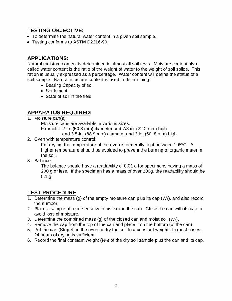
TESTING OBJECTIVE: • To determine the natural water content in a given soil sample. • Testing conforms to ASTM D2216-90. APPLICATIONS: Natural moisture content is determined in almost all soil tests. Moisture content also called water content is the ratio of the weight of water to the weight of soil solids. This ration is usually expressed as a percentage. Water content will define the status of a soil sample. Natural moisture content is used in determining: • Bearing Capacity of soil • Settlement • State of soil in the field APPARATUS REQUIRED: 1. Moisture can(s):

Moisture cans are available in various sizes. Example: 2-in. (50.8 mm) diameter and 7/8 in. (22.2 mm) high

and 3.5-in. (88.9 mm) diameter and 2 in. (50..8 mm) high 2. Oven with temperature control:

For drying, the temperature of the oven is generally kept between 105°C. A higher temperature should be avoided to prevent the burning of organic mater in the soil.

3. Balance: The balance should have a readability of 0.01 g for specimens having a mass of 200 g or less. If the specimen has a mass of over 200g, the readability should be 0.1 g

TEST PROCEDURE: 1. Determine the mass (g) of the empty moisture can plus its cap (W1), and also record

the number. 2. Place a sample of representative moist soil in the can. Close the can with its cap to

avoid loss of moisture. 3. Determine the combined mass (g) of the closed can and moist soil (W2). 4. Remove the cap from the top of the can and place it on the bottom (of the can). 5. Put the can (Step 4) in the oven to dry the soil to a constant weight. In most cases,

24 hours of drying is sufficient. 6. Record the final constant weight (W3) of the dry soil sample plus the can and its cap.

2

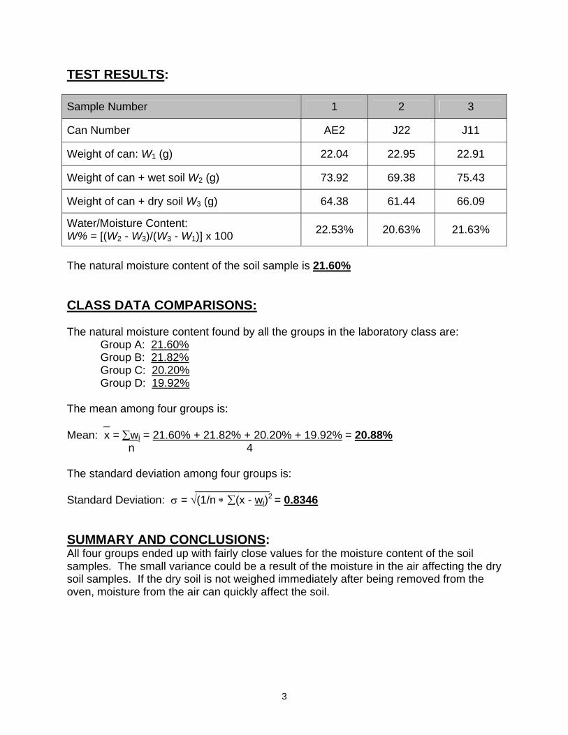
TEST RESULTS: Sample Number 1 2 3

Can Number AE2 J22 J11

Weight of can: W1 (g) 22.04 22.95 22.91

Weight of can + wet soil W2 (g) 73.92 69.38 75.43

Weight of can + dry soil W3 (g) 64.38 61.44 66.09

Water/Moisture Content: W% = [(W2 - W3)/(W3 - W1)] x 100 22.53% 20.63% 21.63%

The natural moisture content of the soil sample is 21.60% CLASS DATA COMPARISONS: The natural moisture content found by all the groups in the laboratory class are:

Group A: 21.60% Group B: 21.82% Group C: 20.20% Group D: 19.92%

The mean among four groups is: _ Mean: x = ∑wi = 21.60% + 21.82% + 20.20% + 19.92% = 20.88% n 4 The standard deviation among four groups is: ____________ Standard Deviation: σ = √(1/n ∗ ∑(x - wi)2 = 0.8346 SUMMARY AND CONCLUSIONS: All four groups ended up with fairly close values for the moisture content of the soil samples. The small variance could be a result of the moisture in the air affecting the dry soil samples. If the dry soil is not weighed immediately after being removed from the oven, moisture from the air can quickly affect the soil.

3

DETERMINATION OF SPECIFIC GRAVITY OF SOIL

EXPERIMENT # 2

CE 3143 September 2, 2003


4

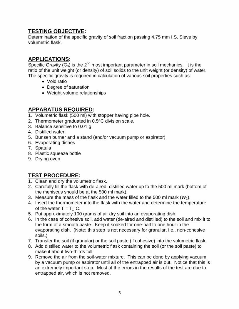
TESTING OBJECTIVE: Determination of the specific gravity of soil fraction passing 4.75 mm I.S. Sieve by volumetric flask. APPLICATIONS: Specific Gravity (Gs) is the 2nd most important parameter in soil mechanics. It is the ratio of the unit weight (or density) of soil solids to the unit weight (or density) of water. The specific gravity is required in calculation of various soil properties such as:

• Void ratio • Degree of saturation • Weight-volume relationships

APPARATUS REQUIRED: 1. Volumetric flask (500 ml) with stopper having pipe hole. 2. Thermometer graduated in 0.5°C division scale. 3. Balance sensitive to 0.01 g. 4. Distilled water. 5. Bunsen burner and a stand (and/or vacuum pump or aspirator) 6. Evaporating dishes 7. Spatula 8. Plastic squeeze bottle 9. Drying oven TEST PROCEDURE: 1. Clean and dry the volumetric flask. 2. Carefully fill the flask with de-aired, distilled water up to the 500 ml mark (bottom of

the meniscus should be at the 500 ml mark). 3. Measure the mass of the flask and the water filled to the 500 ml mark (W1). 4. Insert the thermometer into the flask with the water and determine the temperature

of the water T = T1°C. 5. Put approximately 100 grams of air dry soil into an evaporating dish. 6. In the case of cohesive soil, add water (de-aired and distilled) to the soil and mix it to

the form of a smooth paste. Keep it soaked for one-half to one hour in the evaporating dish. (Note: this step is not necessary for granular, i.e., non-cohesive soils.)

7. Transfer the soil (if granular) or the soil paste (if cohesive) into the volumetric flask. 8. Add distilled water to the volumetric flask containing the soil (or the soil paste) to

make it about two-thirds full. 9. Remove the air from the soil-water mixture. This can be done by applying vacuum

by a vacuum pump or aspirator until all of the entrapped air is out. Notice that this is an extremely important step. Most of the errors in the results of the test are due to entrapped air, which is not removed.

5

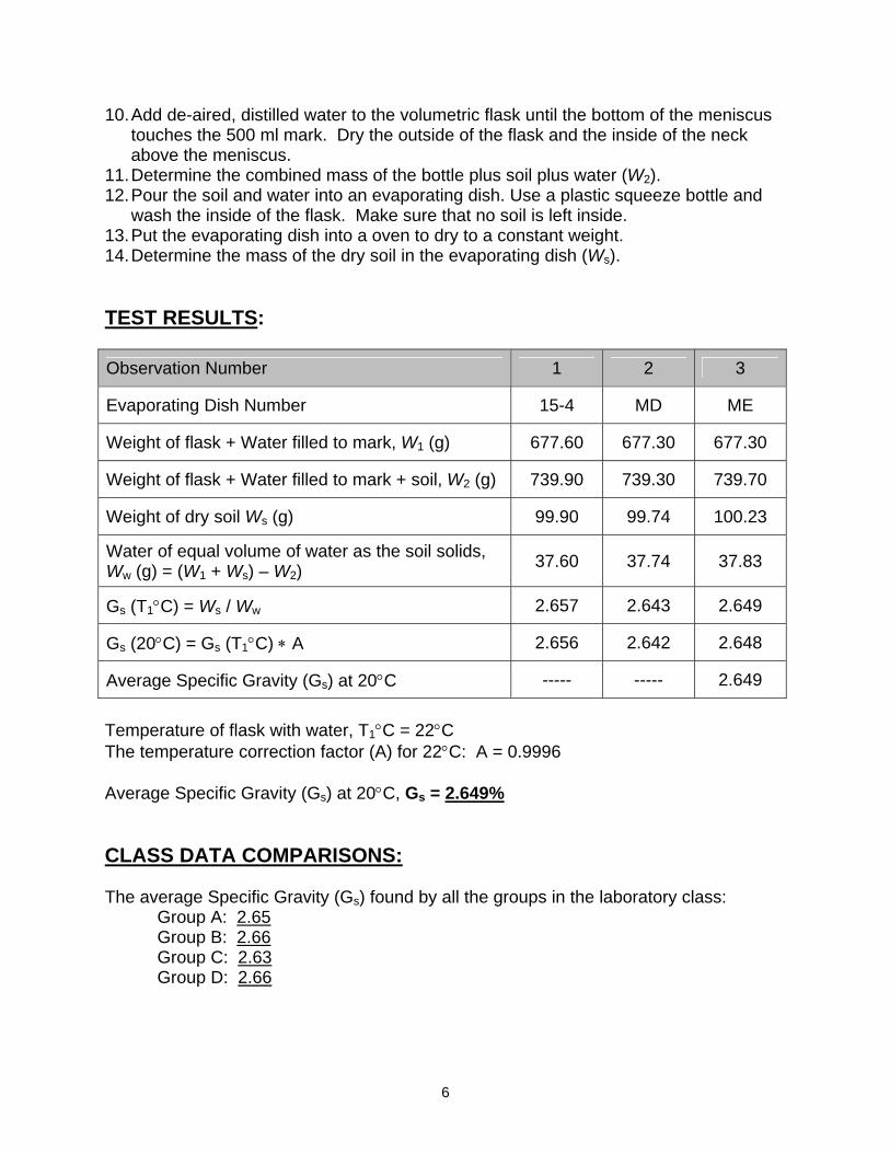
10. Add de-aired, distilled water to the volumetric flask until the bottom of the meniscus touches the 500 ml mark. Dry the outside of the flask and the inside of the neck above the meniscus.

11. Determine the combined mass of the bottle plus soil plus water (W2). 12. Pour the soil and water into an evaporating dish. Use a plastic squeeze bottle and

wash the inside of the flask. Make sure that no soil is left inside. 13. Put the evaporating dish into a oven to dry to a constant weight. 14. Determine the mass of the dry soil in the evaporating dish (Ws). TEST RESULTS: Observation Number 1 2 3

Evaporating Dish Number 15-4 MD ME

Weight of flask + Water filled to mark, W1 (g) 677.60 677.30 677.30

Weight of flask + Water filled to mark + soil, W2 (g) 739.90 739.30 739.70

Weight of dry soil Ws (g) 99.90 99.74 100.23

Water of equal volume of water as the soil solids, Ww (g) = (W1 + Ws) – W2)

37.60 37.74 37.83

Gs (T1°C) = Ws / Ww 2.657 2.643 2.649

Gs (20°C) = Gs (T1°C) ∗ A 2.656 2.642 2.648

Average Specific Gravity (Gs) at 20°C ----- ----- 2.649 Temperature of flask with water, T1°C = 22°C The temperature correction factor (A) for 22°C: A = 0.9996 Average Specific Gravity (Gs) at 20°C, Gs = 2.649% CLASS DATA COMPARISONS: The average Specific Gravity (Gs) found by all the groups in the laboratory class:

Group A: 2.65 Group B: 2.66 Group C: 2.63 Group D: 2.66

6

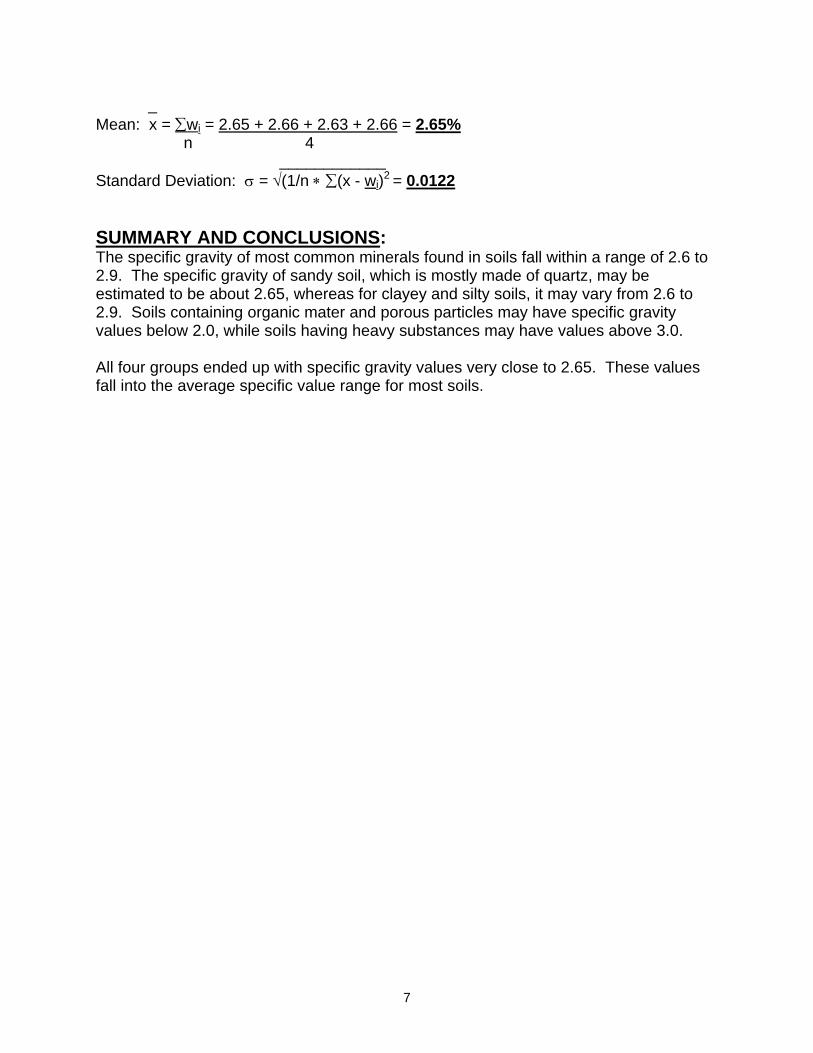
_ Mean: x = ∑wi = 2.65 + 2.66 + 2.63 + 2.66 = 2.65% n 4 ____________ Standard Deviation: σ = √(1/n ∗ ∑(x - wi)2 = 0.0122 SUMMARY AND CONCLUSIONS: The specific gravity of most common minerals found in soils fall within a range of 2.6 to 2.9. The specific gravity of sandy soil, which is mostly made of quartz, may be estimated to be about 2.65, whereas for clayey and silty soils, it may vary from 2.6 to 2.9. Soils containing organic mater and porous particles may have specific gravity values below 2.0, while soils having heavy substances may have values above 3.0. All four groups ended up with specific gravity values very close to 2.65. These values fall into the average specific value range for most soils.

7

GRAIN SIZE DISTRIBUTION SIEVE ANALYSIS

EXPERIMENT # 3



8

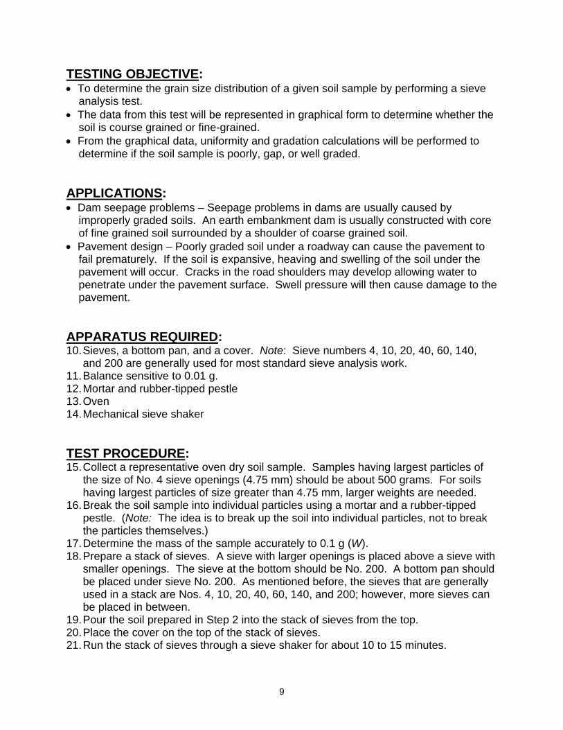
TESTING OBJECTIVE: • To determine the grain size distribution of a given soil sample by performing a sieve analysis test. • The data from this test will be represented in graphical form to determine whether the soil is course grained or fine-grained. • From the graphical data, uniformity and gradation calculations will be performed to determine if the soil sample is poorly, gap, or well graded. APPLICATIONS:• Dam seepage problems – Seepage problems in dams are usually caused by improperly graded soils. An earth embankment dam is usually constructed with core of fine grained soil surrounded by a shoulder of coarse grained soil. • Pavement design – Poorly graded soil under a roadway can cause the pavement to fail prematurely. If the soil is expansive, heaving and swelling of the soil under the pavement will occur. Cracks in the road shoulders may develop allowing water to penetrate under the pavement surface. Swell pressure will then cause damage to the pavement. APPARATUS REQUIRED: 10. Sieves, a bottom pan, and a cover. Note: Sieve numbers 4, 10, 20, 40, 60, 140,

and 200 are generally used for most standard sieve analysis work. 11. Balance sensitive to 0.01 g. 12. Mortar and rubber-tipped pestle 13. Oven 14. Mechanical sieve shaker TEST PROCEDURE: 15. Collect a representative oven dry soil sample. Samples having largest particles of

the size of No. 4 sieve openings (4.75 mm) should be about 500 grams. For soils having largest particles of size greater than 4.75 mm, larger weights are needed.

16. Break the soil sample into individual particles using a mortar and a rubber-tipped pestle. (Note: The idea is to break up the soil into individual particles, not to break the particles themselves.)

17. Determine the mass of the sample accurately to 0.1 g (W). 18. Prepare a stack of sieves. A sieve with larger openings is placed above a sieve with

smaller openings. The sieve at the bottom should be No. 200. A bottom pan should be placed under sieve No. 200. As mentioned before, the sieves that are generally used in a stack are Nos. 4, 10, 20, 40, 60, 140, and 200; however, more sieves can be placed in between.

19. Pour the soil prepared in Step 2 into the stack of sieves from the top. 20. Place the cover on the top of the stack of sieves. 21. Run the stack of sieves through a sieve shaker for about 10 to 15 minutes.

9

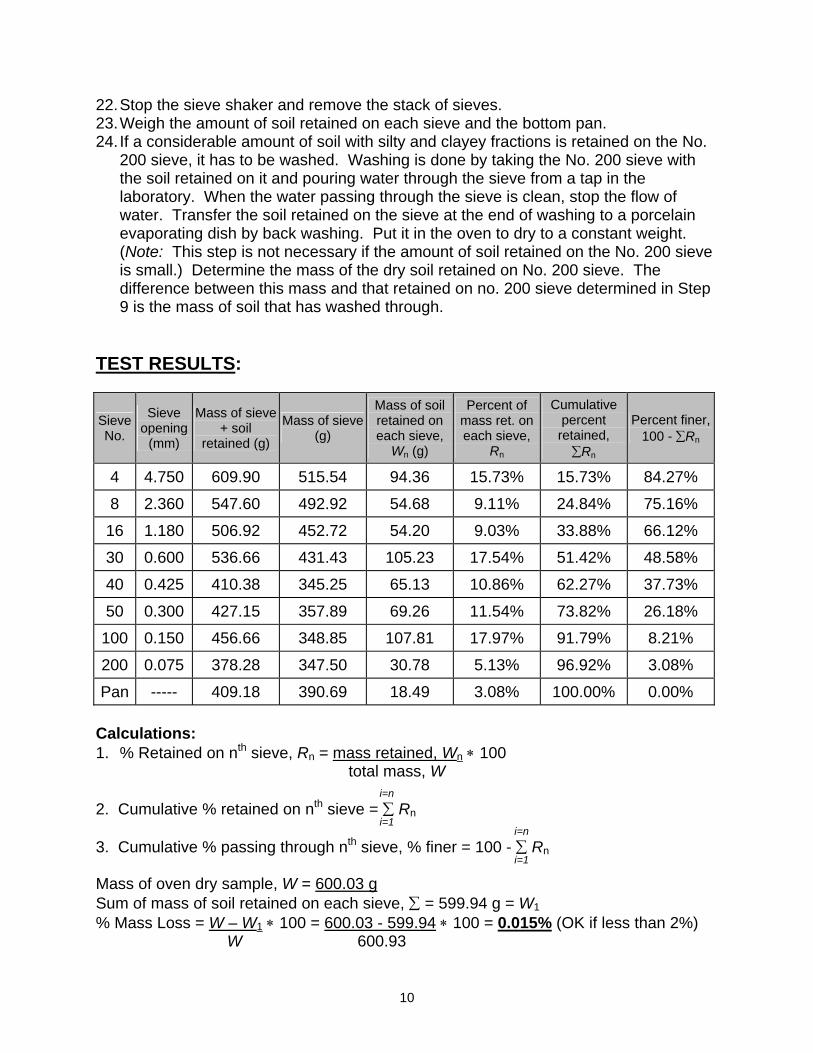
22. Stop the sieve shaker and remove the stack of sieves. 23. Weigh the amount of soil retained on each sieve and the bottom pan. 24. If a considerable amount of soil with silty and clayey fractions is retained on the No.

200 sieve, it has to be washed. Washing is done by taking the No. 200 sieve with the soil retained on it and pouring water through the sieve from a tap in the laboratory. When the water passing through the sieve is clean, stop the flow of water. Transfer the soil retained on the sieve at the end of washing to a porcelain evaporating dish by back washing. Put it in the oven to dry to a constant weight. (Note: This step is not necessary if the amount of soil retained on the No. 200 sieve is small.) Determine the mass of the dry soil retained on No. 200 sieve. The difference between this mass and that retained on no. 200 sieve determined in Step 9 is the mass of soil that has washed through.

TEST RESULTS:

Sieve No.

Sieve opening

(mm)

Mass of sieve + soil

retained (g)

Mass of sieve (g)

Mass of soil retained on each sieve,

Wn (g)

Percent of mass ret. on each sieve,

Rn

Cumulative percent retained, ∑Rn

Percent finer, 100 - ∑Rn

4 4.750 609.90 515.54 94.36 15.73% 15.73% 84.27%

8 2.360 547.60 492.92 54.68 9.11% 24.84% 75.16%

16 1.180 506.92 452.72 54.20 9.03% 33.88% 66.12%

30 0.600 536.66 431.43 105.23 17.54% 51.42% 48.58%

40 0.425 410.38 345.25 65.13 10.86% 62.27% 37.73%

50 0.300 427.15 357.89 69.26 11.54% 73.82% 26.18%

100 0.150 456.66 348.85 107.81 17.97% 91.79% 8.21%

200 0.075 378.28 347.50 30.78 5.13% 96.92% 3.08%

Pan ----- 409.18 390.69 18.49 3.08% 100.00% 0.00% Calculations: 1. % Retained on nth sieve, Rn = mass retained, Wn ∗ 100

total mass, W i=n 2. Cumulative % retained on nth sieve = ∑ Rn

i=1 i=n 3. Cumulative % passing through nth sieve, % finer = 100 - ∑ Rn i=1

Mass of oven dry sample, W = 600.03 gSum of mass of soil retained on each sieve, ∑ = 599.94 g = W1 % Mass Loss = W – W1 ∗ 100 = 600.03 - 599.94 ∗ 100 = 0.015% (OK if less than 2%)

W 600.93

10

From the graph, the percents finer of 10%, 30%, and 60%, which are respectively, the diameters D10, D30, and D60 are: From the graph, the percents finer of 10%, 30%, and 60%, which are respectively, the diameters D D10 = 0.17 D

10, D30, and D60 are:

D30 = 0.35 D10 = 0.17

D60 = 0.90 D30 = 0.35 60 = 0.90

Uniformity Coefficient (Cu) = D60 / D10 = 0.90 / 0.17 = 5.29 Uniformity Coefficient (C

u) = D60 / D10 = 0.90 / 0.17 = 5.29

Coefficient of Gradation (Cc) = D302 / (D60 ∗ D10) = (0.35)2 / (0.90 ∗ 0.17) = 0.801 Coefficient of Gradation (Cc) = D302 / (D60 ∗ D10) = (0.35)2 / (0.90 ∗ 0.17) = 0.801

CLASS DATA COMPARISONS: CLASS DATA COMPARISONS:

Group A Group A Group B Group B Group C Group C Group D Group D

D10 0.17 0.17 0.18 0.18 0.19 0.19 0.17 0.17

D30 0.35 0.35 0.38 0.38 0.37 0.37 0.33 0.33

D60 0.90 0.90 1.20 1.20 0.90 0.90 0.98 0.98

D10

D30

D60

11 11

Mean: x = ∑wi = n D10 = 0.178 D30 = 0.358 D60 = 0.995 ____________ Standard Deviation: σ = √(1/n ∗ ∑(x - wi)2

D10 = 0.008290 D30 = 0.01920 D60 = 0.1228 SUMMARY AND CONCLUSIONS: The most basic classification of soil is whether it is fine-grained (cohesive), or coarse-grained (non-cohesive). Soils offer two types of resistance, plasticity (c) and friction (φ). For fine-grained soils, the resistance comes from plasticity which is when the particles in a soil stick together. Resistance in coarse-grained soils comes from friction. An ideal soil is a well-graded soil with the qualities of both fine and coarse-grained soils. The method of soil gradation or grain size distribution for coarse-grained soils is the sieve analysis test. For fine-grained soils, the hydrometer test is used. From the sieve analysis test, over 80% of the soil sample is sand, while some 15% is gravel, and 3% is fines (silt and clay). With the majority soil sample consisting of sandy particles, the soil type can be classified as sand with some fines (silt and clay). Three numerical values were read directly from the particle-size distribution curve; the diameters, D10, D30, and D60. The diameter D10 is generally referred to as the effective size. From these values the Uniformity Coefficient (Cu) and the Coefficient of Gradation (Cc) can be calculated. The Uniformity Coefficient (Cu) is a parameter which indicates the range of distribution of grain sizes in a given soil sample. For well-graded soils Cu is large, usually greater than 6 for sandy soils. Poorly graded soils have Cu that is nearly equal to 1, which means that the soil particles are approximately equal in size. The Coefficient of Gradation (Cc) is a parameter that is also referred to as the coefficient of curvature. For soil to be considered well-graded Cc is usually between 1 and 3. The soil sample tested with the sieve analysis test in the laboratory has properties that come very close to the general requirements and properties of a well-graded soil. The Uniformity Coefficient (Cu) was found to be 5.29, which is close to 6 for sandy soils. The Coefficient of Gradation (Cc) was found to be 0.801, which is close to 1 for sandy soils. The graph of the sieve analysis particle-size distribution curve closely resembles an example of a well-graded soil. From the calculated and graphical data it can be determined that the soil sample is a well-graded sandy soil with some fines.

12

GRAIN SIZE DISTRIBUTION HYDROMETER ANALYSIS

EXPERIMENT # 4



13

TESTING OBJECTIVE: • To determine the particle-size distribution of a given soil sample for the fraction that is finer than No. 200 sieve size (0.075 mm). The lower limit of the particle-size determined by this procedure is about 0.001 mm. • In hydrometer analysis, a soil specimen is dispersed in water. In a dispersed state in the water, the soil particles will settle at different velocities over time. • The hydrometer will measure the specific gravity of the soil-water suspension. • Hydrometer readings will be taken at specific time intervals to measure the percentage of soil still in suspension at time t. • From this data the percentage of soil by weight finer and the diameters (D) of the soil particles at their respective time readings can be calculated. • A graph of the diameter (D) vs. percent finer can be plotted to develop a particle-size distribution curve. APPLICATIONS:• In many cases, the results of the sieve analysis and hydrometer analysis of a given soil sample are combined on one graph. When these results are combined on one graph, a discontinuity occurs because soil particles are generally irregular in shape. • Hydrometer test is used to determine what type of clay is predominant in a given soil sample (Ex: kaoloinite, illite, montmorillonite, etc…) APPARATUS REQUIRED: 15. ASTM 152-H hydrometer 16. Mixer 17. Two 100-cc graduated cylinders 18. Thermometer 19. Constant temperature bath 20. Deflocculating agent 21. Spatula 22. Beaker 23. Balance 24. Plastic squeeze bottle 25. Distilled water 26. No. 12 rubber stopper

14

TEST PROCEDURE: Note: This procedure is used when more than 90 percent of the soil is finer than No. 200 sieve. 25. Take 50 g of oven-dry, well-pulverized soil in a beaker. 26. Prepare a deflocculating agent. Usually a 4% solution of sodium

hexametaphosphate (Calgon) is used. This can be prepared by adding 40 g of Calgon in 1000 cc of distilled water and mixing it thoroughly.

27. Take 125 cc of the mixture prepared in Step 2 and add it to the soil taken in Step 1. This should be allowed to soak for about 8 to 12 hours.

28. Take a 1000-cc graduated cylinder and add 875 cc of distilled water pluts 125 cc of deflocculating agent in it. Mix the solution well.

29. Put the cylinder (from Step 4) in a constant temperature bath. Record the temperature of the bath, T (in °C).

30. Put the hydrometer in the cylinder (Step 5). Record the reading. (Note: The top of the meniscus should be read.) This is the zero correction (Fz), which can be +ve or -ve. Also observe the meniscus correction (Fm).

31. Using a spatula, thoroughly mix the soil prepared in Step 3. Pour it into the mixer5 cup. Note: During this process, some soil may stick to the side of the beaker. Using the plastic squeeze bottle filled with distilled water, wash all the remaining soil in the beaker into the mixer cup.

32. Add distilled water to the cup to make it about two-thirds full. Mix it for about two minutes using the mixer.

33. Pour the mix into the second graduated 1000-cc cylinder. Make sure that all of the soil solids are washed out of the mixer cup. Fill the graduated cylinder with distilled water to bring the water level up to the 1000-cc mark.

34. Secure a No. 12 rubber stopper on the top of the cylinder (Step 9). Mix the soil-water well by turning the soil cylinder upside down several times.

35. Put the cylinder into the constant temperature bath next to the cylinder described in Step 5. Record the time immediately. This is cumulative time t=0. Insert the hydrometer into the cylinder containing the soil-water suspension.

36. Take hydrometer readings at cumulative times t=0.25 min., 0.5 min., 1 min., and 2 min. Always read the upper level of the meniscus.

37. Take the hydrometer out after two minutes and put it in the cylinder next to it(Step 5) 38. Hydrometer readings are to be taken at time t=4 min., 8 min., 15 min., 30 min., 1 hr.,

2 hr., 4 hr., 8 hr., 24 hr., and 48 hr. For each reading, insert the hydrometer into the cylinder containing the soil-water suspension about 30 seconds before the reading is due. After the reading is taken, remove the hydrometer and put it back into the cylinder next to it (Step 5).

15

TEST RESULTS:

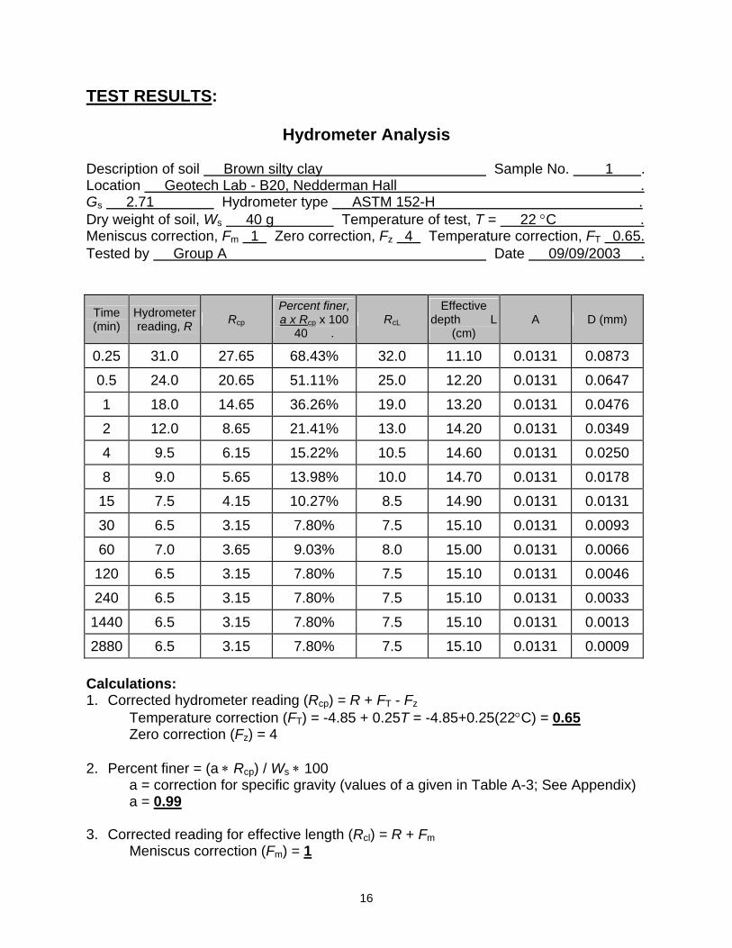
Hydrometer Analysis Description of soil Brown silty clay Sample No. 1 . Location Geotech Lab - B20, Nedderman Hall . Gs 2.71 Hydrometer type ASTM 152-H . Dry weight of soil, Ws 40 g Temperature of test, T = 22 °C .Meniscus correction, Fm 1 Zero correction, Fz 4 Temperature correction, FT 0.65. Tested by Group A Date 09/09/2003 .

Time (min)

Hydrometer reading, R Rcp

Percent finer, a x Rcp x 100

40 . RcL

Effective depth L

(cm) A D (mm)

0.25 31.0 27.65 68.43% 32.0 11.10 0.0131 0.0873

0.5 24.0 20.65 51.11% 25.0 12.20 0.0131 0.0647

1 18.0 14.65 36.26% 19.0 13.20 0.0131 0.0476

2 12.0 8.65 21.41% 13.0 14.20 0.0131 0.0349

4 9.5 6.15 15.22% 10.5 14.60 0.0131 0.0250

8 9.0 5.65 13.98% 10.0 14.70 0.0131 0.0178

15 7.5 4.15 10.27% 8.5 14.90 0.0131 0.0131

30 6.5 3.15 7.80% 7.5 15.10 0.0131 0.0093

60 7.0 3.65 9.03% 8.0 15.00 0.0131 0.0066

120 6.5 3.15 7.80% 7.5 15.10 0.0131 0.0046

240 6.5 3.15 7.80% 7.5 15.10 0.0131 0.0033

1440 6.5 3.15 7.80% 7.5 15.10 0.0131 0.0013

2880 6.5 3.15 7.80% 7.5 15.10 0.0131 0.0009 Calculations: 1. Corrected hydrometer reading (Rcp) = R + FT - Fz

Temperature correction (FT) = -4.85 + 0.25T = -4.85+0.25(22°C) = 0.65Zero correction (Fz) = 4

2. Percent finer = (a ∗ Rcp) / Ws ∗ 100 a = correction for specific gravity (values of a given in Table A-3; See Appendix) a = 0.99

3. Corrected reading for effective length (Rcl) = R + Fm

Meniscus correction (Fm) = 1

16

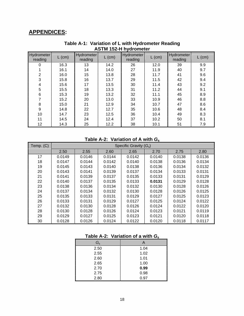
4. Effective Length (L) = (values of L given in Table A-1; See Appendix) 5. Variation of (A) with Gs and T°C = (values of A given in Table A-2; See Appendix)

_____________ 6. Particle Diameter D (mm) = A√(L(cm) / t (min))

SUMMARY AND CONCLUSIONS: The hydrometer test for the given soil sample produced results for very small particles as expected. The particle size distribution curve shows values ranging from 0.085mm (close to No. 200 sieve) to 0.00095mm. There is however, a variation in the curve at around 0.02 mm. This is likely because the hydrometer reading at 1 hr. was 0.5 higher than the reading before it at 30 min. and the reading after it at 2 hr.

17

APPENDICES:

Table A-1: Variation of L with Hydrometer Reading ASTM 152-H hydrometer

Hydrometer reading L (cm) Hydrometer

reading L (cm) Hydrometer reading L (cm) Hydrometer

reading L (cm)

0 16.3 13 14.2 26 12.0 39 9.9 1 16.1 14 14.0 27 11.9 40 9.7 2 16.0 15 13.8 28 11.7 41 9.6 3 15.8 16 13.7 29 11.5 42 9.4 4 15.6 17 13.5 30 11.4 43 9.2 5 15.5 18 13.3 31 11.2 44 9.1 6 15.3 19 13.2 32 11.1 45 8.9 7 15.2 20 13.0 33 10.9 46 8.8 8 15.0 21 12.9 34 10.7 47 8.6 9 14.8 22 12.7 35 10.6 48 8.4 10 14.7 23 12.5 36 10.4 49 8.3 11 14.5 24 12.4 37 10.2 50 8.1 12 14.3 25 12.2 38 10.1 51 7.9

Table A-2: Variation of A with GsTemp. (C) Specific Gravity (Gs)

2.50 2.55 2.60 2.65 2.70 2.75 2.80 17 0.0149 0.0146 0.0144 0.0142 0.0140 0.0138 0.0136 18 0.0147 0.0144 0.0142 0.0140 0.0138 0.0136 0.0134 19 0.0145 0.0143 0.0140 0.0138 0.0136 0.0134 0.0132 20 0.0143 0.0141 0.0139 0.0137 0.0134 0.0133 0.0131 21 0.0141 0.0139 0.0137 0.0135 0.0133 0.0131 0.0129 22 0.0140 0.0137 0.0135 0.0133 0.0131 0.0129 0.0128 23 0.0138 0.0136 0.0134 0.0132 0.0130 0.0128 0.0126 24 0.0137 0.0134 0.0132 0.0130 0.0128 0.0126 0.0125 25 0.0135 0.0133 0.0131 0.0129 0.0127 0.0125 0.0123 26 0.0133 0.0131 0.0129 0.0127 0.0125 0.0124 0.0122 27 0.0132 0.0130 0.0128 0.0126 0.0124 0.0122 0.0120 28 0.0130 0.0128 0.0126 0.0124 0.0123 0.0121 0.0119 29 0.0129 0.0127 0.0125 0.0123 0.0121 0.0120 0.0118 30 0.0128 0.0126 0.0124 0.0122 0.0120 0.0118 0.0117

Table A-2: Variation of a with GsGs A

2.50 1.04 2.55 1.02 2.60 1.01 2.65 1.00 2.70 0.99 2.75 0.98 2.80 0.97

18

ATTERBERG LIMIT TESTS LIQUID LIMIT & PLASTIC LIMIT

EXPERIMENT # 5



19

TESTING OBJECTIVE: • To determine the Atterberg Limits/Consistency Limits and classify the soil from the plasticity chart. The Atterberg Limits are a method to describe the consistency of fine-grained soils. Two of these limits are the Plastic Limit and the Liquid Limit. From these values the Plasticity Index may be calculated. • Plastic Limit (PL) - the moisture content of a soil at the point of transition from semisolid to plastic state. • Liquid Limit (LL) - the moisture content of a soil at the point of transition from plastic to liquid state. • Plasticity Index (PI) – the difference between the Liquid Limit and the Plastic Limit. PI = LL - PL. APPLICATIONS:• Consistency limits (LL and PL) are significant to understand the stress history and general properties of the soil met with construction. An estimate of Plasticity Index is important to classify the soils particularly in highly expansive clays. • High PI soils are more difficult to compact. The sometimes need to be stabilized by chemicals. • Low PI soils make construction difficult, because adding only a little water turns the soil to liquid (LL).

A) LIQUID LIMIT TEST APPARATUS REQUIRED: 27. Casagrande liquid limit device 28. Grooving tool 29. Mixing dishes 30. Spatula 31. Balance Sensitive up to 0.01 g 32. Electric Oven TEST PROCEDURE: 1. Determine the mass of each of the three moisture cans (W1). 2. Make sure to calibrate the drop of the cup using the other edge of the grooving tool

so that there is a consistency in height of drop. 3. Put about 250 g of air dried soil passing # 40 into an evaporating dish and add a little

water with a plastic squeeze bottle to barely form a paste like consistency. 4. Place the soil in the Casagrande’s cup and using a spatula, smoothen the surface so

that the maximum depth is about 8mm. 5. Using the grooving tool, cut a grove at the center line of the soil pat. 6. Crank the device at a rate of 2 revolutions per second until there is a clear visible

closure of ½” or 12.7 mm in the soil pat placed in the cup. Count the number of

20

blows (N) that caused the closure (make the paste so that N begins with a value higher than 35).

7. If N ~ 20 to 40, collect the sample from the closed part of the pat using a spatula and determine the water content weighing the weight of the can + moist soil (W2). If the soil is too dry, N will be higher and reduces as water is being added.

8. Additional soil shouldn’t be added to make the soil dry, expose the mix to a fan or dry it by continuously mixing it with the spatula.

9. CLEAN THE CUP AFTER EACH TRIAL, obtain a minimum of three trials with values of N ~ 20 to 40.

10. Determine the corresponding w% after 24 hrs and plot the N vs w%, called the “flow curve”.

TEST RESULTS:

Liquid Limit Test No. 1 2 3 Can No. 1 2 3

Mass of can, W1 (g) 89.15 80.18 105.66

Mass of can + moist soil, W2 (g) 97.77 90.72 115.42

Mass of can + dry soil, W3 (g) 96.31 88.90 113.68

Moisture content, w(%) = W2 - W3 x 100 . W3 - W1

20.39% 20.87% 21.70%

Number of blows, N 43 35 22

21

Calculations: 7. Liquid Limit (LL) = 21.5 8. Flow Index (F1) = w1(%) - w2(%) = 21.70 - 20.39 = 4.50

log N2 – log N1 log43 - log22

B) PLASTIC LIMIT TEST

APPARATUS REQUIRED: 1. Mixing dishes 2. Spatula 3. Balance Sensitive up to 0.01 g 4. TxDOT recommended Plastic limit device (for this session). TEST PROCEDURE: 1. Take approximately 20 g of dry soil and mix some amount of water from the plastic

squeeze bottle. 2. Determine the weight of empty moisture can, (W1). 3. Prepare several small, ellipsoidal rolls of soil and place them in the plastic limit

device. Place two fresh sheets of filter papers on either faces of the plates. 4. Roll the upper half of the device which has a calibrated opening of 3.18 mm with the

lower half plate. 5. If the soil gets crumbled forming a thread of about the size of the opening between

the plates, collect the crumbled sample, weigh it in the moisture can (W2) for water content determination. Otherwise repeat the test with the same soil but drying it by squeezing between your palms.

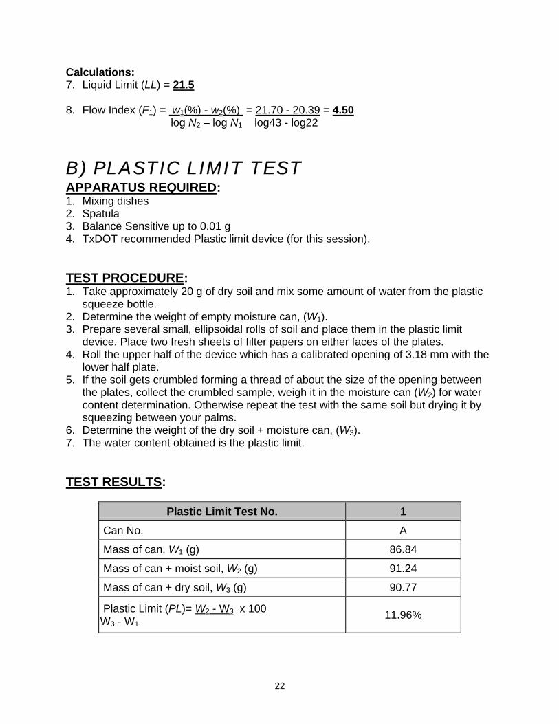
6. Determine the weight of the dry soil + moisture can, (W3). 7. The water content obtained is the plastic limit. TEST RESULTS:

Plastic Limit Test No. 1 Can No. A

Mass of can, W1 (g) 86.84

Mass of can + moist soil, W2 (g) 91.24

Mass of can + dry soil, W3 (g) 90.77

Plastic Limit (PL)= W2 - W3 x 100 W3 - W1

11.96%

22

Calculations: 1. Plastic Limit (PL) = 11.96 2. Liquid Limit (LL) = 21.50 (from part A) 3. Plasticity Index (PI) = LL - PL = 21.50 - 11.96 = 9.54

Plastictiy Chart

0

10

20

30

40

50

60

70

0 10 20 30 40 50 60 70 80 90 100

Liquid Limit

Plas

ticity

Inde

x

CL

ML

CH

MH

U-LINE

A-LINE

CL-ML

SOILSAMPLE

CLASS DATA COMPARISONS: Group A Group B Group C Group D

Liquid Limit 21.50 20.80 19.98 21.28

Plastic Limit 11.96 10.50 9.60 5.93

Plasticity Index 9.54 10.30 10.38 15.35

23

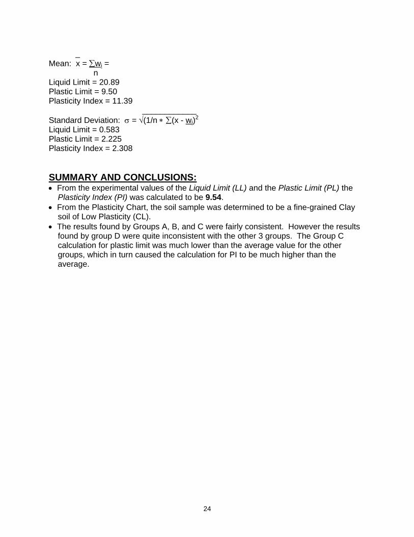
_ Mean: x = ∑wi = n Liquid Limit = 20.89 Plastic Limit = 9.50 Plasticity Index = 11.39 ____________ Standard Deviation: σ = √(1/n ∗ ∑(x - wi)2

Liquid Limit = 0.583 Plastic Limit = 2.225 Plasticity Index = 2.308 SUMMARY AND CONCLUSIONS:• From the experimental values of the Liquid Limit (LL) and the Plastic Limit (PL) the Plasticity Index (PI) was calculated to be 9.54. • From the Plasticity Chart, the soil sample was determined to be a fine-grained Clay soil of Low Plasticity (CL). • The results found by Groups A, B, and C were fairly consistent. However the results found by group D were quite inconsistent with the other 3 groups. The Group C calculation for plastic limit was much lower than the average value for the other groups, which in turn caused the calculation for PI to be much higher than the average.

24

physical and plasticity characteristics - · pdf filephysical and plasticity characteristics...

Documents