physical principles of remote sensing - earth online

Dr. Claudia Künzer Dr. Claudia Künzer

Physical Principles of Remote Sensing

Dr. Claudia Kuenzer German Remote Sensing Data Center, DFD German Aerospace Center, DLR email: [email protected] fon: +49 – 8153 – 28-3280

Thermal Remote Sensing


Thermal Infrared Remote Sensing

§ TIR at high Resolution (Thermal Camera)

Theoretical Background

Dr. Claudia Künzer

Radiation at wavelengths between 3 - 14 µm

All materials at temperatures above absolute zero (0 K, -273°C) continuously emit electromagnetic radiation. The earth with its ambient temperature of ca. 300 K has its peak energy emission in the thermal infrared region at around 9.7 µm.

Source: http://bigfootproof.com/groups/visible-invisible-d2-ranges.html


Thermal Infrared Radiation


Dr. Claudia Künzer

Atmospheric Windows in the Thermal IR Region situated between 3 - 5 µm and

8 - 14 µm. The latter has narrow absorption band from 9 to 10 µm caused by ozone, which is omitted by most thermal IR satellite sensors. Note that reflected sunlight can contaminate thermal IR signals recorded in the 3 - 5 µm windows during daytime. Source: Sabins (1997)



Dr. Claudia Künzer

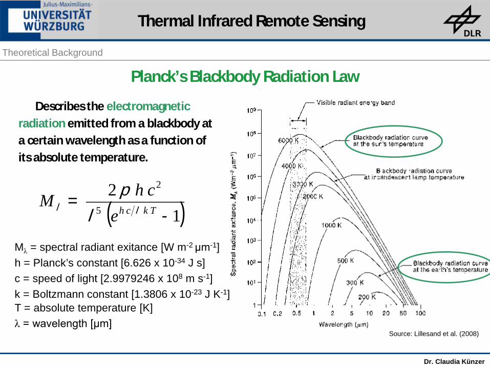
Planck’s Blackbody Radiation Law Describes the electromagnetic radiation emitted from a blackbody at a certain wavelength as a function of its absolute temperature.

( )12

5

2

-=

TkchechM

ll lp

Source: Lillesand et al. (2008)

Mλ = spectral radiant exitance [W m-2 μm-1] h = Planck’s constant [6.626 x 10-34 J s] c = speed of light [2.9979246 x 108 m s-1] k = Boltzmann constant [1.3806 x 10-23 J K-1] T = absolute temperature [K] λ = wavelength [μm]



Dr. Claudia Künzer

Stefan-Boltzmann Law

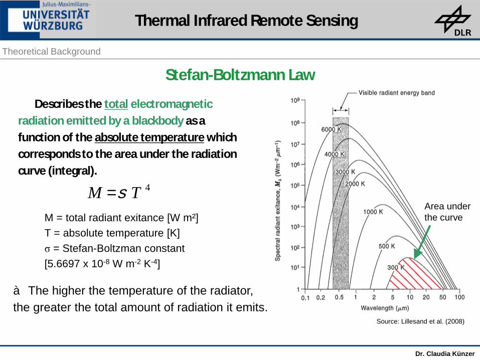
Describes the total electromagnetic radiation emitted by a blackbody as a function of the absolute temperature which corresponds to the area under the radiation curve (integral).

4TM s=M = total radiant exitance [W m²] T = absolute temperature [K] σ = Stefan-Boltzman constant [5.6697 x 10-8 W m-2 K-4]

à The higher the temperature of the radiator, the greater the total amount of radiation it emits.

Area under the curve




Dr. Claudia Künzer

Wien‘s Displacement Law

Describes the wavelength at which the maximum spectral radiant exitance occurs.

TA

=maxl

λmax = wavelength of maximum spectral radiant exitance [μm] A = Wien‘s constant [2897.8 μm K] T = absolute temperature [K]

à With increasing temperature λmax

shifts to shorter wavelengths. Source: Lillesand et al. (2008)

Maximum spectral radiant exitance



Dr. Claudia Künzer

VIS versus SWIR Landsat 7 ETM+ 14. Feb. 2000, Kilauea Volcano (Hawaii)

False color composite

(RGB, 7 5 4)

True color composite

(RGB, 3 2 1)



Dr. Claudia Künzer

SWIR versus TIR

Gray scale Band 6

Gray scale Band 7


Landsat 7 ETM+ 14. Feb. 2000, Kilauea Volcano (Hawaii)


Dr. Claudia Künzer

Interaction of Radiation with Terrain Elements

1=++ lll tra

α, ρ, τ are wavelength dependent and represent ratios between the absorbed, reflected and transmitted components of the incident energy striking a terrain element and the total energy incident on the terrain element, respectively.

absorbed radiation (α)

transmitted radiation (τ)

reflected radiation (ρ) incoming radiation



Dr. Claudia Künzer

Blackbody Concept

A blackbody is a hypothetical, ideal radiator that totally absorbs and re-emits all energy incident upon it. The total energy a blackbody radiates and the spectral distribution of the emitted energy (radiation curve) depends on the temperature of the blackbody and can be described by:

Planck’s radiation law

Stefan-Boltzmann law

Wien’s displacement law


absorbed radiation emitted radiation


Dr. Claudia Künzer

Radiation of real Materials and Emissivity

Real materials do not behave like blackbodies. They emit only a fraction of the radiation emitted by a blackbody at the equivalent temperature. This is taken into account by the EMISSIVITY, or the emissivity coefficient (ε):

Emissivity can have values between 0 and 1. It is a measure of the ability of a material both to radiate and to absorb energy.

etemperatur same the atblackbody a ofexitanceradiantetemperatur given a at object an ofexitanceradiant

=le


M = total radiant exitance [W m²] T = absolute temperature [K σ = Stefan-Boltzman constant]


Dr. Claudia Künzer

Kirchhoff’s Radiation Law

Since most objects are opaque (do not let radiation transmit) to thermal infrared radiation (τλ = 0):

à The higher an object’s reflectance in the thermal IR region, the lower its emissivity and vice versa.

1=++ lll tre

1=+ ll re

According to Kirchhoff’s radiation law:

Spectral emissivity of an black body object equals its spectral absorbance: “good absorbers are good emitters” On the basis of Kirchhoff’s radiation law αλ can be replaced with ελ:

ll ae =


(for a blackbody)


Dr. Claudia Künzer

Provided that the emissivity of a material is known, its absolute temperature (kinetic temperature, Tkin) can be derived from the radiation it emits. If the emissivity is not considered, only the brightness temperature (radiant temperature, Trad) of the material can be determined. Since it is valid that:

kinrad TT e=

kinrad TT =

the radiant temperature of a real material is always lower than its kinetic temperature. However, for a blackbody with ε = 1 it applies that:


!!! Radiation of real Materials !!!

sensed touched


Dr. Claudia Künzer

Radiation of real Materials

Emissivity depends on wavelength, surface temperature, and some physical properties of the surface, e.g. water content, or density.

Material Average Emissivity over 8-14 μm

Clear water 0.98 - 0.99 Healthy green vegetation 0.96 - 0.99 Dry vegetation 0.88 - 0.94 Asphaltic concrete 0.94 - 0.97 Basaltic rock 0.92 - 0.96 Granitic rock 0.83 - 0.87 Dry mineral soil 0.92 - 0.96 Polished metals 0.06 - 0.21 So

urce

: Lille

sand

et a

l. (2

008)



Dr. Claudia Künzer


Because of emissivity different objects can have the same kinetic temperature but differ significantly in the radiation they emit and their radiant temperatures !!!

Source: Sabins (1997)



kinrad TT 41e=

Dr. Claudia Künzer

Radiation of real Materials visible (left) vs. thermal IR (right), Sacramento, CAL, USA



Dr. Claudia Künzer

Changes in Emissivity of Surfaces ……

Actually should be taken into Account for any urban heat island related analyses in fast growing cities




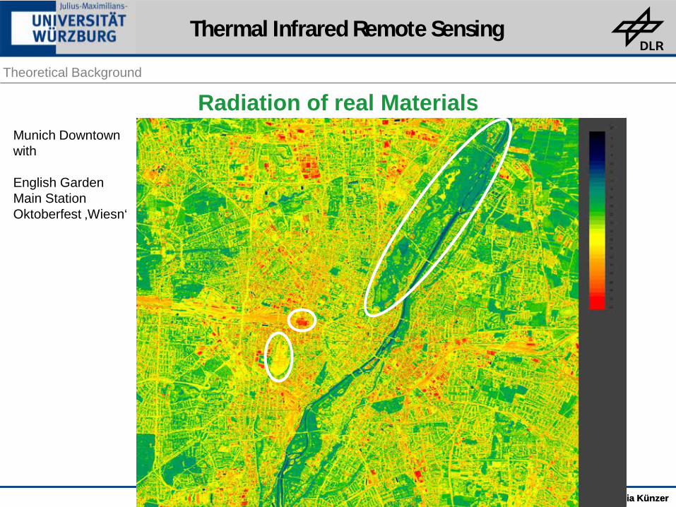
Radiation of real Materials Theoretical Background

Munich Downtown with English Garden Main Station Oktoberfest ‚Wiesn‘


Dr. Claudia Künzer


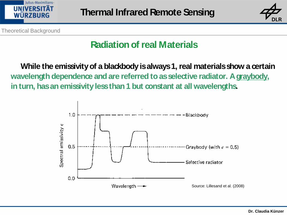
While the emissivity of a blackbody is always 1, real materials show a certain wavelength dependence and are referred to as selective radiator. A graybody, in turn, has an emissivity less than 1 but constant at all wavelengths.




Dr. Claudia Künzer


When broadband sensors are used emissivity for any given material type is often considered to be constant in the 8 - 14 µm range, which means these materials are treated as graybodies (but e.g. ASTER ….).




Dr. Claudia Künzer


Emissivity spectra of different igneous rocks. Arrows show centers of adsorption bands. Spectra are offset vertically (Source: Sabins 1997).



Dr. Claudia Künzer

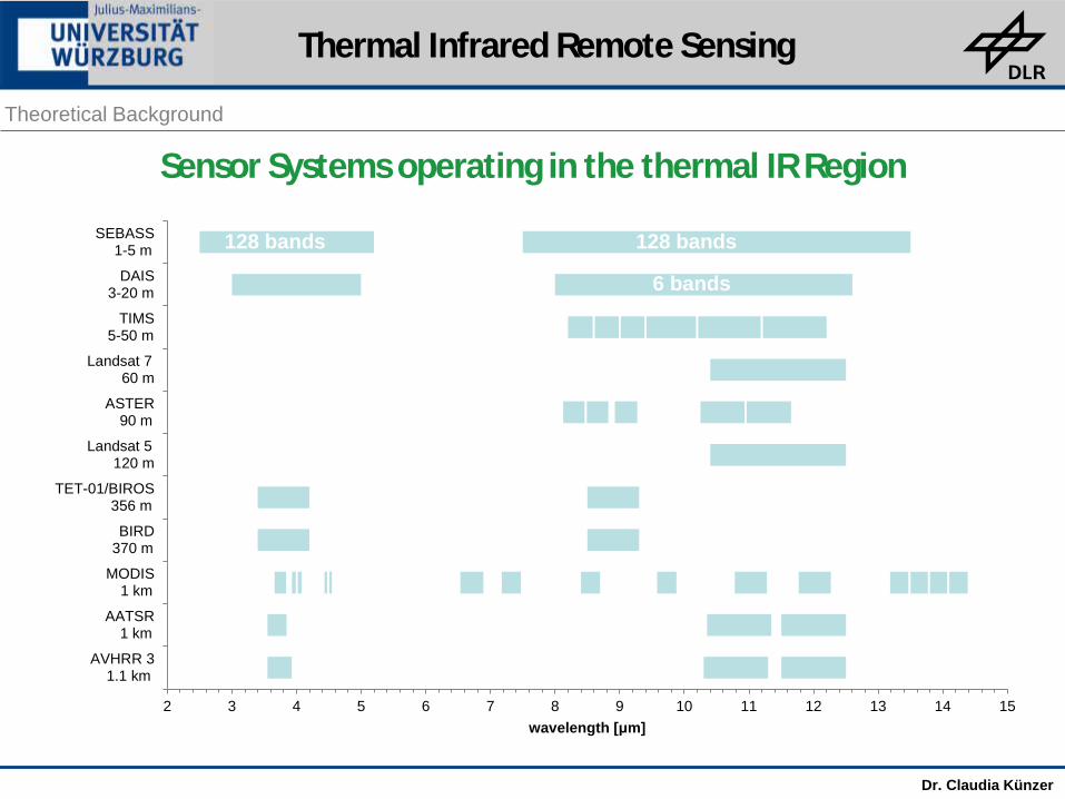
2 3 4 5 6 7 8 9 10 11 12 13 14 15

AVHRR 3 1.1 km

AATSR 1 km

MODIS 1 km

BIRD370 m

TET-01/BIROS 356 m

Landsat 5 120 m

ASTER 90 m

Landsat 7 60 m

TIMS5-50 m

DAIS 3-20 m

SEBASS 1-5 m

wavelength [μm]

Sensor Systems operating in the thermal IR Region

128 bands 128 bands

6 bands



Dr. Claudia Künzer

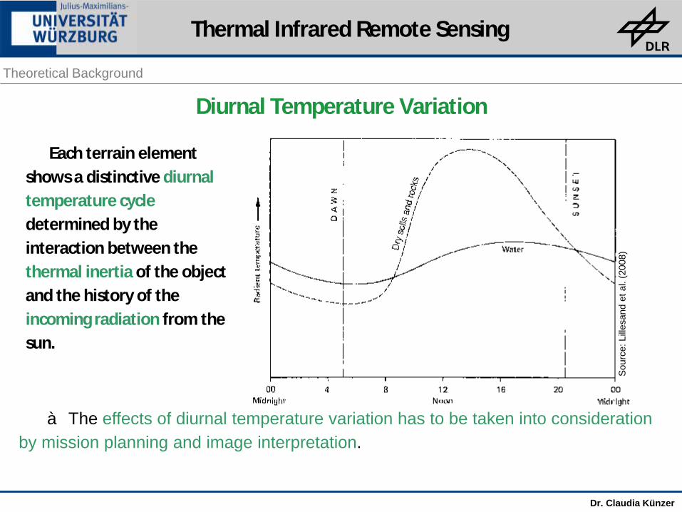
Diurnal Temperature Variation

Each terrain element shows a distinctive diurnal temperature cycle determined by the interaction between the thermal inertia of the object and the history of the incoming radiation from the sun.

à The effects of diurnal temperature variation has to be taken into consideration by mission planning and image interpretation.

Sour

ce: L

illesa

nd e

t al.

(200

8)



Dr. Claudia Künzer

Diurnal Temperature Variation

Daytime

Sour

ce: L

illesa

nd e

t al.

(200

8)

Nighttime

Middleton (WI), USA



Dr. Claudia Künzer

Diurnal Temperature Variation and Solar Effects Day/Night

Sour

ce: S

abin

s (1

997)

Nighttime

Caliente and Temblor Ranges (CAL), USA

Daytime




Intra-Annual Temperature Variation Theoretical Background


Dr. Claudia Künzer

Thermal Inertia Thermal inertia: measure of the resistance of a material to temperature changes.

In general, materials with high thermal inertia have more uniform surface temperatures throughout the day and night than material of low thermal inertia

The difference between maximum and minimum temperature occurring during a diurnal solar cycle is called ΔT (Sabins 1997).

Source: Sabins (1997)



Dr. Claudia Künzer

Apparent Thermal Inertia

Materials with low thermal inertia have a relatively high ΔT. The opposite is true for materials with high thermal inertia. ΔT can be derived by subtracting the minimum nighttime temperature from the maximum daytime temperature of two images covering the same area. Then the apparent thermal inertia (ATI) can be calculated by:

TAATI

D-

=1

A is the albedo in the visible band and compensates for the effects that differences in absorptivity have on radiant temperature.



Dr. Claudia Künzer

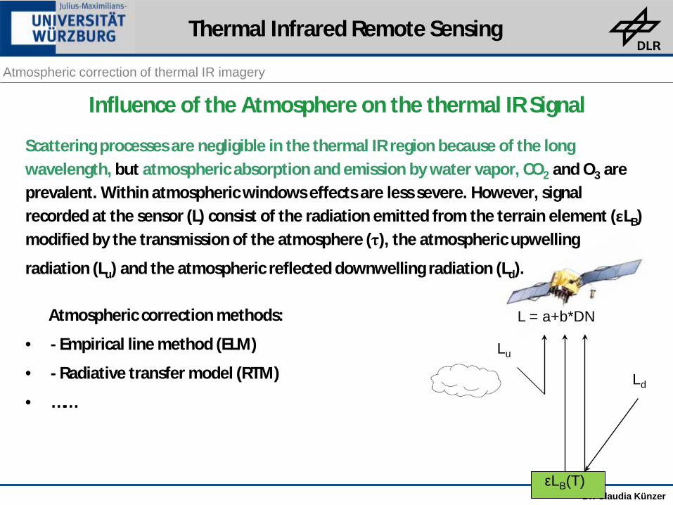
Influence of the Atmosphere on the thermal IR Signal

Scattering processes are negligible in the thermal IR region because of the long wavelength, but atmospheric absorption and emission by water vapor, CO2 and O3 are prevalent. Within atmospheric windows effects are less severe. However, signal recorded at the sensor (L) consist of the radiation emitted from the terrain element (εLB) modified by the transmission of the atmosphere (τ), the atmospheric upwelling

radiation (Lu) and the atmospheric reflected downwelling radiation (Ld). Atmospheric correction methods:

• - Empirical line method (ELM)

• - Radiative transfer model (RTM)

• ……

εLB(T)

Lu

Ld

L = a+b*DN

Atmospheric correction of thermal IR imagery


Dr. Claudia Künzer

Empirical Line Method (ELM)

ELM applies a linear regression to each band by plotting DN or at-satellite reflectance (Lλ) values against in-situ temperature measurements recorded simultaneous with satellite overpass. The resulting coefficients a (offset) and b (gain) are used to transform each pixel value in the scene to its kinetic temperature (Tk).

Drawback:

in-situ measurements are cost intensive, time-consuming and not available for remote areas or images from the past

DN or Lλ

Tk

a (intercept)

b (slope)

DNbaTk *+=

in-situ temperature measurements



Dr. Claudia Künzer

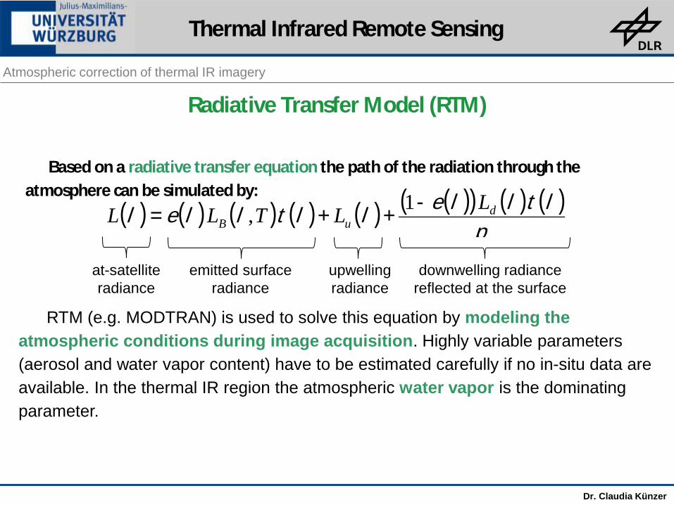
Radiative Transfer Model (RTM)

Based on a radiative transfer equation the path of the radiation through the atmosphere can be simulated by:

( ) ( ) ( ) ( ) ( ) ( )( ) ( ) ( )p

ltllelltllel duB

LLTLL -++=

1,

at-satellite radiance

emitted surface radiance

upwelling radiance

downwelling radiance reflected at the surface

RTM (e.g. MODTRAN) is used to solve this equation by modeling the atmospheric conditions during image acquisition. Highly variable parameters (aerosol and water vapor content) have to be estimated carefully if no in-situ data are available. In the thermal IR region the atmospheric water vapor is the dominating parameter.




Summary of Theory


Thermal remote sensing data needs to be treated differently from other remote sensing data, most important are the laws of Planck, Boltzmann, Kirchhoff and Wien

Proper preprocessing: Data must first be atmospherically corrected

Derived temperatures need to be corrected for the emissivity effect, this is usually done with the support of precise landcover classificatiosn data

When comparing multi date imagery diurnal effects must be considered, thermal pixel values cannot be compared as easily as multispectral values

Materials with a high thermal inertia have a less accentuated diurnal cycle, materials with a low thermal inertia show a much larger variability (e.g. water, metal), synthetic ATI images can help in the differentiation of materials with similar spectral properties



Publication: Frey C.M., Kuenzer C., Dech S. (2012): Quantitative comparison of the operational NOAA AVHRR LST product of DLR and the MODIS LST product V005. International Journal of Remote Sensing. Vol. 33, No. 22, 7165-7183

Operational AVHRR LST Composites for Europe


Diurnal Temperature Variations

à LST shows an extremely high diurnal variation à The variation of LST is higher than the variation of air temperatures à Figure: up to 4 K difference in LST per hour (mean values of three month)


à in extreme and sloped terrain even up to > 10°C à LST differences depend on aspect

Diurnal Temperature Variations


Geographical coverage for AVHRR data reception from Oberpfaffenhofen, Germany (www.eoweb.de)

The NOAA-AVHRR-LST Product: a Composite


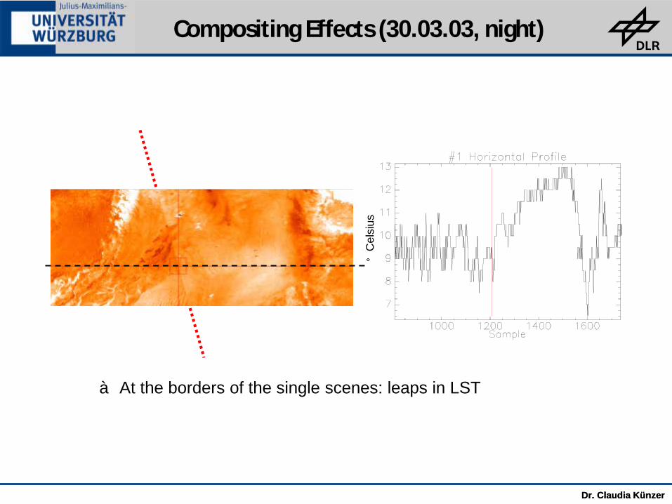
°C

elsi

us

à At the borders of the single scenes: leaps in LST

Compositing Effects (30.03.03, night)


NOAA-AVHRR LST often miss Metadata

Pixelwise time of acquisition Only the day of acquisition is given in the metadata. However, due to the

compositing techniques and the wide swath width, local times of single pixels may differ considerably

Pixelwise acquisition angle Usually, no information about the acquisition angle is given. The acquisition angle however is important due to thermal anisotropy (BRDF) Quality information No information about the quality of the acquisitions for a given pixel is

provided Emissivity The emissivity is calculated via the NDVI and not delivered as a separate

layer. This missing data complicates the interpretation and validation of the data.


Consequences: - The missing metadata (time of acquisition, acquisition angle,

quality information, emissivity) complicates the interpretation of the data considerably.

The data – as it is – cannot be used as model input, e.g. for climate models

There is a need to investigate the product concerning its accuracy.

NOAA-AVHRR LST often miss Metadata


Cross-Comparison AVHRR-LST / MODIS-LST

Cross comparison of AVHRR LST and MODIS LST c5 daily (day and night scenes)

- Comparison pixelwise for selected pixels - Acquisition time difference: daytime 5 minutes, nighttime 30

minutes allowed - Acquisition time is not available for AVHRR, therefore this had

to be reconstructed - Only ‚spatial homogeneous‘ pixels were chosen.

Four years, each containing only data of one NOAA satellite:

2003 à only NOAA-16 scenes




Data generated by other NOAA-Satellites were eliminated


Geographical coverage for AVHRR data reception from Oberpfaffenhofen, Germany (www.eoweb.de)

The NOAA-AVHRR-LST Product: a Composite


Longitudinal variation

+ =

Local time of the subsatellite track, calculated from the starting time t0 and the acquisition velocity of AVHRR

Local time

t0

Time

à Input data: Generated positions of the raw scenes à Output: Layer giving the acquisition time pixelwise (local time)

Calculation of pixelwise Acquisition Time


MODIS west MODIS east

AVHRR Europe Filter:

1. Pixels in areas

without path overlaps

2. Low variability of NDVI and LST inside a 5x5 pixel environment

3. 250m SRTM DEM slope is < 2°

à Homogeneous pixels are mostly found in North Africa

AVHRR LST – Homogeneous Pixels


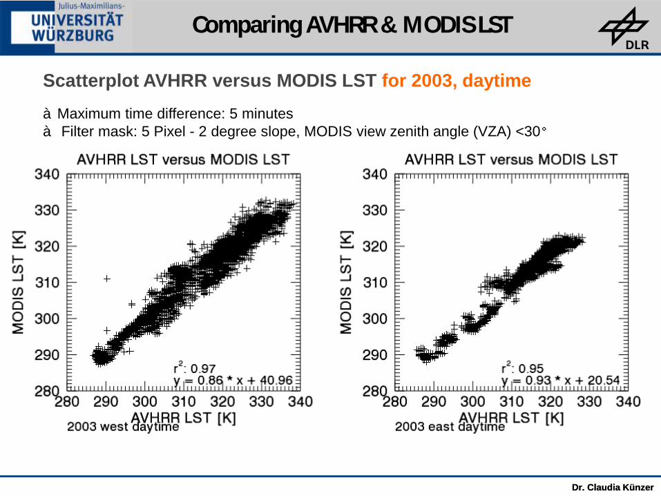
Scatterplot AVHRR versus MODIS LST for 2003, daytime àMaximum time difference: 5 minutes à Filter mask: 5 Pixel - 2 degree slope, MODIS view zenith angle (VZA) <30°

Comparing AVHRR & MODIS LST


Scatterplot AVHRR versus MODIS LST for all Years and all Scenes àMaximum time difference: 5 minutes for daytime, 30 for nighttime scenes à Filter mask: 5 Pixel - 2 degree slope, MODIS view zenith angle (VZA) <30°

r2: 0.980

Daytime Nighttime

r2: 0.962



3 pixel 3 degree 5 pixel 2 degree 7 pixel 2 degree

Scatterplot Differences AVHRR versus MODIS LST and Homogenity of Area (2003, 2010)

à Impact of homogenity criteria àFiltermask: 2 degree slope à MODIS VZA<30°, varying homogeneous areas

MAD: 2.49

MAD: 3.22 MAD: 2.70

MAD: 2.46 MAD: 2.43

MAD: 3.83

Kein Filter

MAD: 3.17

MAD: 5.22



Scatterplot Difference AVHRR versus MODIS LST depending on MODIS VZA

à Influence of the VZA of MODIS à (only every 10th pixel plotted) à Filtermask: 5 Pixel - 2 degree slope

<50° <40° <30° MODIS VZA

Different VZA have a strong impact on the differences



Scatterplot AVHRR versus MODIS LST for the Year 2010, nighttime

àMaximum time difference: 30 Minutes à Filtermask: 5 Pixel – 2 degree slope, MODIS VZA<30°

Checked for all years: Slope is for all 4

investigated years and in both areas < 1 à with high LSTs AVHRR shows higher values

than MODIS



Cross-Comparison of NOAA-AVHRR LST and MODIS LST Day and night with and without homogenity critera

2D histograms of AVHRR and MODIS LST for all four years, both MODIS tiles, day- and nighttimes. Only pixels with viewing angles lower than 30°were used and the maximal time difference was 5 min for the daytime scenes, 30 min for the nighttime scenes. a) with no homogeneity filter applied b) with the homogeneity filter applied.



Diurnal Mean absolute Difference (MAD) per Day and Tile between AVHRR and MODIS LST

MAD of the Egyptian tile in 2003 daytimeFilter: 5 pixel - 2 degree

-1

1

3

5

7

9

11

13

15

10. Dez. 28. Feb. 19. Mai. 7. Aug. 26. Okt. 14. Jan. 3. Apr.

Date

MA

D

All pixel Maximal 30 Min difference Maximal 5 Min time difference

Daytime - MODIS VZA<30°



-1

1

3

5

7

9

11

13

15

10. Dez. 28. Feb. 19. Mai. 7. Aug. 26. Okt. 14. Jan. 3. Apr.

MA

D

Date

MAD of the Moroccan tile in 2003 nighttimeFilter: 5 pixel - 2 degree

All pixel Maximal 30 Min time difference

Nighttime - MODIS VZA<50°

Diurnal Mean absolute Difference (MAD) per Day and Tile between AVHRR and MODIS LST



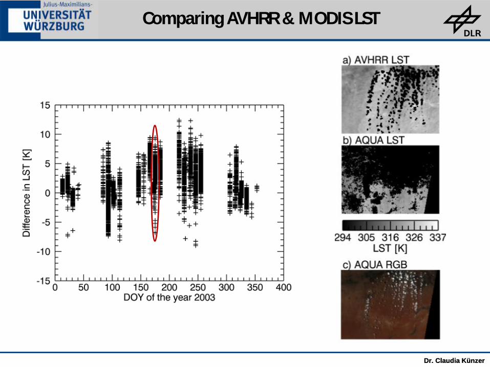
Daytime Differences (AVHRR LST – MODIS LST)


Nighttime Differences (AVHRR – MODIS )

The differences show a clear annual behavious. Maximum differences can be found during daytime in summer.

Dr. Claudia Künzer

Statistics of the data after elimination of acquisition angles > 30deg., time differences higher than 5 minutes (daytime scenes) / 30 minutes (nighttime scenes) and inhomogeneous pixels

MAD [K] Slope Correlation coeffizient r2

Daytime 2.2 0.89 0.96

Nighttime 1.4 0.88 0.98

à Good agreement between the two datasets!


Frey C.M., Kuenzer C., Dech S. (2012): Quantitative comparison of the operational NOAA AVHRR LST product of DLR and the MODIS LST product V005. International Journal of Remote Sensing. 33:22, 7165-7183


à Only a strict selection of pixels allowing only certain acquisition time differences, homogeneity of the pixels and view zenith angle enables an optimal comparison between AVHRR LST and MODIS LST

à Mean aboslute difference MAD per scene and year ranges from 1.4 to 3.2 K (daytime scenes) and from 0.9 to 2.2 K (nighttime scenes).

à A distinct annual course was found in the daytime data. Highest differences are found in summer, which may considerably exceed mean annual MADs.

à A weak annual course is found in the nighttime data.

Summary: Results of the scientific Comparison


Application: Remote Sensing of Coal Fire Environments




Coal Fires in China: Introduction

Spontaneous combustion: C + O2 >> CO2 + 394 KJ/mol 2C + O2 >> 2CO + 170 KJ/mol




coalfires

Coal Fires: An International Problem Application: Remote Sensing of Coal Fire Environments



Coal Fires: An International Problem

• Environmental Problems • Gas Emissions (CO2, CH4, others) • Land subsidence and cracks • Threat to human health • Regional landscape degradation

• Economic Problems

• In China: 20 Mio. t coal loss / year • Coal fire research needs funding • Deserted mining towns; migrations




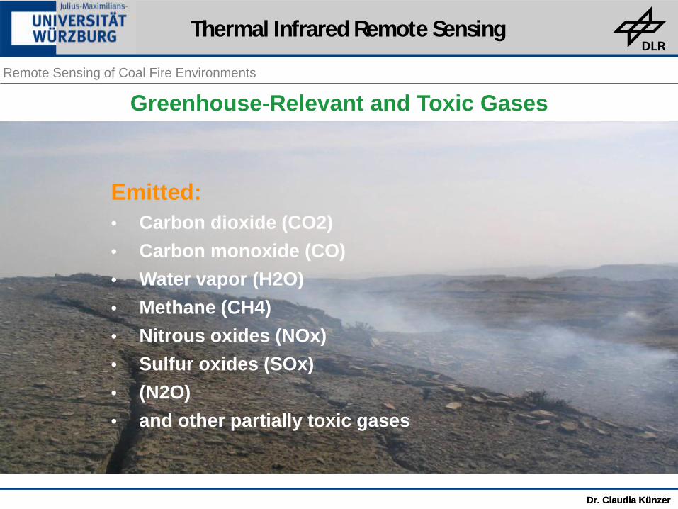
Greenhouse-Relevant and Toxic Gases Remote Sensing of Coal Fire Environments

Emitted: • Carbon dioxide (CO2) • Carbon monoxide (CO) • Water vapor (H2O) • Methane (CH4) • Nitrous oxides (NOx) • Sulfur oxides (SOx) • (N2O) • and other partially toxic gases



Economic Loss of Valuable Resource

• 70% chinese energy covered by coal

• 2 billion t/a mined

• 20-30 million tons burning

• the 10-fold becomes inaccessible

• discrepancy: energy demand / production




Coal Fire Fighting – Challenges Methods: - Digging out and isolating the fires - Water injections for cooling - Covering of fires

Remote Sensing of Coal Fire Environments



Location of Study Areas in Ningxia and Inner Mongolia Remote Sensing of Coal Fire Environments

Orientation Map: Chinese Provinces

Xinjiang

Xizang

Inner Mongolia

Qinghai

Sichuan

Gansu

Jilin

Yunnan

Heilongjiang

Hebei

Hunan

Hubei

Guangxi

HenanAnhui

Shaanxi

Jiangxi

Shanxi

Guizhou Fujian

Liaoning

Shandong

Guangdong

Jiangsu

Zhejiang

Ningxia

Hainan

BeijingTianjin

Shanghai

Hong Kong

25° 25°

35° 35°

45° 45°

55° 55°75°

85°

85°

95°

95°

105°

105°

115°

115°

125°

125°

135°

135°145°

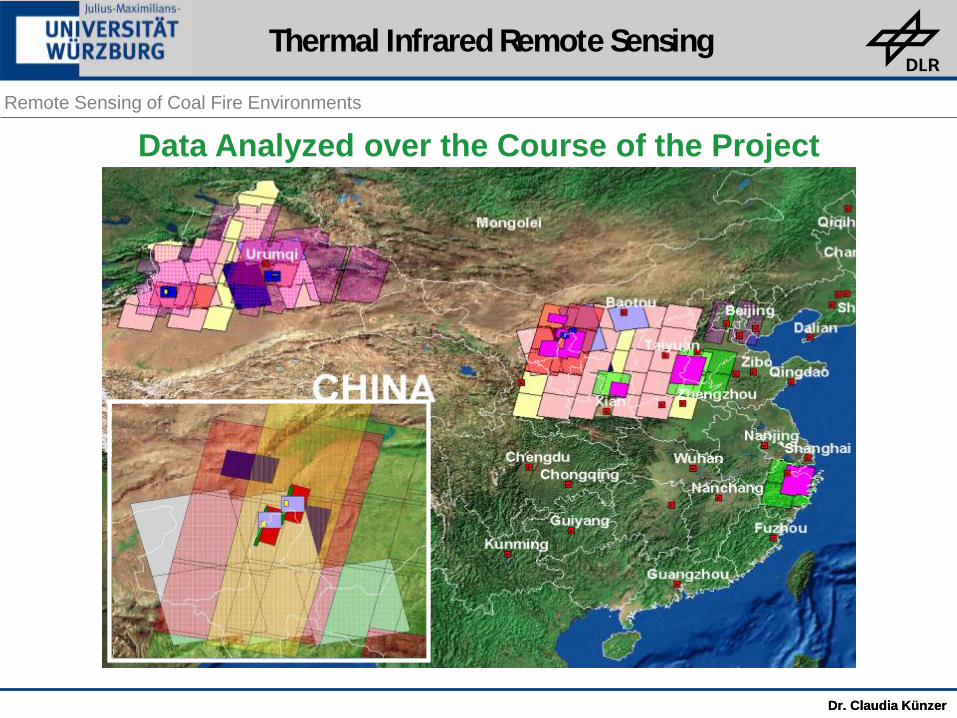
CHINA

Mongolia

NepalButhan India

Myan

marRussia

India

RussiaPacific Ocean

Outcropping coal seams

Coaltown Wuda

Yellow River

Red: vegetation



Chinese mining Town Ruqigou in Ningxia Remote Sensing of Coal Fire Environments



Some Impressions … Remote Sensing of Coal Fire Environments



Data Analyzed over the Course of the Project Remote Sensing of Coal Fire Environments



Thermal Expression of Coal Fires in EO Data Remote Sensing of Coal Fire Environments

Outcropping coal seams

Coal town Wuda

Yellow River

Red: vegetation



Thermal Expression of Coal Fires In-Situ Remote Sensing of Coal Fire Environments



Thermal Characteristics of Coal Fires: WEAK Anomalies (much different from e.g. forest fires !)


Real subsurface coal fire

Simulated surface coal fire

Statistical fire properties: • Fire temparatures strongly varying • Coal fire areas in satellite imagery: high variability • Coal fire areas do not exceed a certain size • Contrast in night time data higher • Contrast in winter data better than in summer data • Solar influence least pre dawn • Surface coal fires give stronger expression

Night: s² bgr. low Fire: contrast higher Day: s² bgr. high Fire: contrast low



Thermal on Site Experiments with different Fires Remote Sensing of Coal Fire Environments

ZHANG, J. and KUENZER, C., 2007: Thermal surface characteristics of coal fires 1: Results of in-situ measurements. Journal of Applied Geophysics, DOI:10.1016/j.jappgeo.2007.08.002, Vol. 63, pp. 117-134

ZHANG, J., KUENZER, C., TETZLAFF, A., OERTL, D., ZHUKOV, B. and WAGNER, W., 2007: Thermal characteristics of coal fires 2: Results of measurements on simulated coal fires. Journal of Applied Geophysics, DOI:10.1016/j.jappgeo.2007.08.003, Vol. 63, pp. 135-147



The capability of MODIS diurnal thermal bands observations

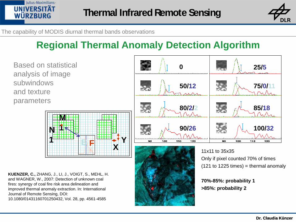
Regional Thermal Anomaly Detection Algorithm

Based on statistical analysis of image subwindows and texture parameters

0

50/12

100/32 90/26

85/18 80/2/2

75/0/11

25/5

11x11 to 35x35 Only if pixel counted 70% of times (121 to 1225 times) = thermal anomaly 70%-85%: probability 1 >85%: probability 2

X Y F B

M1 N

1

KUENZER, C., ZHANG, J., LI, J., VOIGT, S., MEHL, H. and WAGNER, W., 2007: Detection of unknown coal fires: synergy of coal fire risk area delineation and improved thermal anomaly extraction. In: International Journal of Remote Sensing, DOI: 10.1080/01431160701250432, Vol. 28, pp. 4561-4585



Thermal Anomaly Extraction from EO Data Remote Sensing of Coal Fire Environments

Anomalies

Histogram method Moving window filter

Cluster

Grouping

Input image

Neighborhood statistics

Probability map of coal fire anomalies

0

50/12

100/32 90/26

85/18 80/2/2

75/0/11

25/5



Coal Fire Area Demarcation: Present Areas and Risk Areas Remote Sensing of Coal Fire Environments

Coal waste pile fires

Subsurface coal fires

no coal fires

no coal fires

no coal fires

no coal fires

no coal fires

no coal fires

N

Detection of Unknown Fires in 2004

< 5 % of full scene as possible coalfire area new fires detected 4 underground 2 coal waste piles risk areas



Thermal Anomaly Quantification Remote Sensing of Coal Fire Environments

Daytime summer (09-2002), ETM+ tIR

Daytime winter (02-2003), ETM+ tIR

Nighttime summer (09-2002), ETM+ tIR

Daytime summer (09-2002), BIRD

Daytime winter (02-2003), BIRD

Nighttime summer (06-2003), BIRD



(Post-) Kyoto Relevance Remote Sensing of Coal Fire Environments

Simplified Model of the Origin of Greenhouse Gases during Complete and Incomplete Combustion

Complete combustion

1t Coal with 750 kg C

N H O S

O2

2.7t CO2

Incomplete combustion (coal fire)

5.1t CO2 Equivalent

1t Coal with 750 kg C

N H O S

O2

0.18t CH4 1.3t CO2

×21



Gas Temporal Variability – Ventilation Pathways Remote Sensing of Coal Fire Environments



Gas Variability Remote Sensing of Coal Fire Environments

CO [ppm]

Strong wind from NW Low to moderate wind from SE 0

500

1000

1500

3000

4500

6000

7500

9000

10000


Coal Fire Mapping in-situ (2000-2005, 2008) Remote Sensing of Coal Fire Environments

• Every year over 600 to 1000 thermal point measurements • For each fire point maximum, minimum and average temperature • Differentiation in colder and hotter areas • Polygons yearly updated and provided to partners, mines, minng authorities

Fire 10, 2005 Fire 14, 2005



Field Mapping versus Remote Sensing




Changes in Extent within one Year (2004-2005) Remote Sensing of Coal Fire Environments



Changes in Extent within one year (2004-2005) Remote Sensing of Coal Fire Environments




Multi-Sensor Transfer from Landsat to MODIS:

• ASTER à often: ‘occupied’, data not always available • LANDSAT à ETM+ erroneous, new mission soon • NOAA, AATSR etc, only one thermal band

à Suitability of low resolution MODIS data to monitor subtle

coal fire related thermal anomalies ?




The MODIS Sensor: Coverage of the Thermal Domain

• 36 bands, bands 8-36 1km res., Relevant for LST analyses: bands 20-23 (3,66 – 4,08µm) and 31, 32 (10,78 – 12,27µm)

• TERRA (‘99), AQUA (’02) à 4-5 times within 24 hour cycle (diurnal cycle), if large scan angles accepted (overlap frames)

• 4-5 days if nadir (climate rel. bgr. variations over 4 days < than diurnal var.)

• Favorable for hotspot detection within 24 hour cycle: Night. Best: predawn (solar effects least accentuated); Seasonal: early spring or late autumn (or if no-snow-area even winter)

• Data free of charge, some preprocessing needed: bowtie correction, geocorrection with geolocation files, radiance to temp. conversion




Adapted to low resolution MODIS Data

Automatic detection in MODIS pre-dawn data (China) • Coalfires • Industry




Study Area, Data, Research Setup

• Jharia coalfield, largest coalfire globally, 50-100 fires, 1916 first

• 4 Scenes: Feb 2005 (morning, afternoon, evening, predawn)

• band 20 (3,66-3,84µm) and 32 (11,77-12,27µm), furthest apart = good

contrast between 20 (outstanding hot spot signals, few reflected and mainly emitted components) and 32 (representing temp. pattern in common thermal domain, only emitted components)

• Creation of ratio band: 20/32. à pixels with similar emission in both bands = values close to 1. Pixels with relatively greater radiance in 20 yield values > 1. à Ratio of 20/32 enhances very strong hot spots

• Automated algorithm for the detection of relative thermal anomalies




MODIS band 20/32 Ratio Images

• Predawn, 17. Feb. 2005 • b, c: background temp. strong var.

Lighter pixels = higher temps. • Ratio image enhances hot thermal

anomalies as high pixel values and suppresses background variation

Thermal Infrared



Application of the Algorithm to MODIS

• 20, 32 and ratio underwent algorithm

• Output: - Background = black, 0; - Regional anomalies counted 70%-85% of times = grey, 1 - Anomalies counted > 85% of times = white, 2.




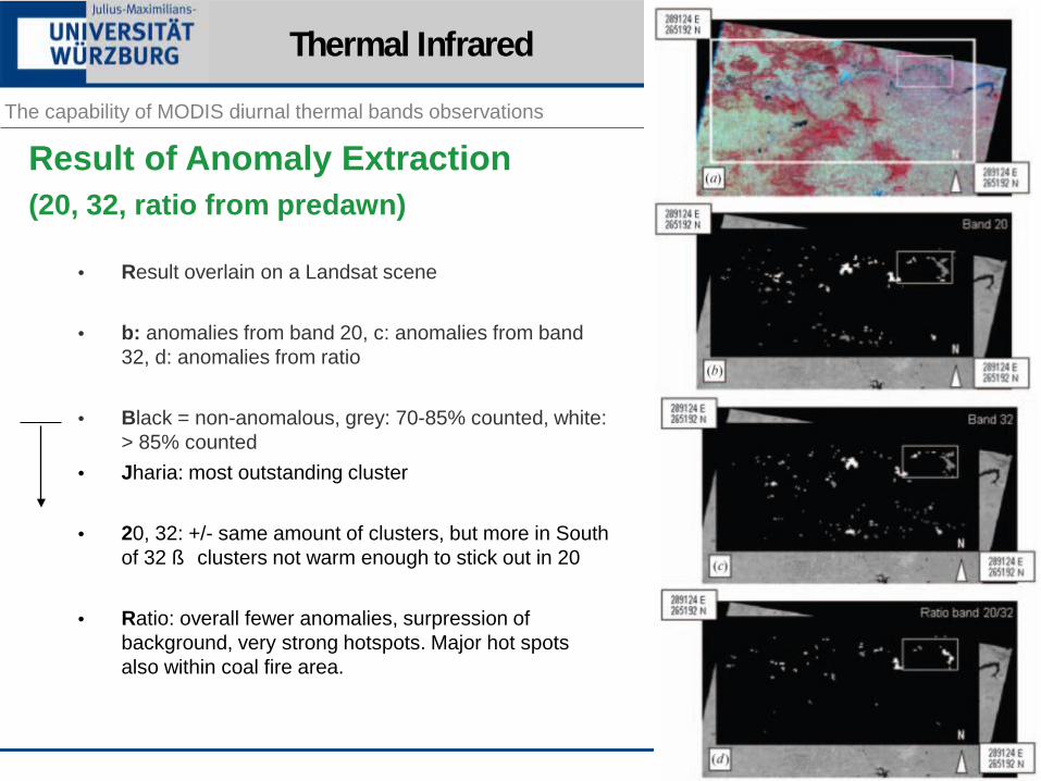
Result of Anomaly Extraction (20, 32, ratio from predawn)

• Result overlain on a Landsat scene

• b: anomalies from band 20, c: anomalies from band 32, d: anomalies from ratio

• Black = non-anomalous, grey: 70-85% counted, white: > 85% counted

• Jharia: most outstanding cluster

• 20, 32: +/- same amount of clusters, but more in South of 32 ß clusters not warm enough to stick out in 20

• Ratio: overall fewer anomalies, surpression of background, very strong hotspots. Major hot spots also within coal fire area.

Thermal Infrared



Extraction from Ratio Band (morning, afternoon, evening, predawn)

• a: morning, b: afternoon, c: evening, d: predawn • Jharia most prominent cluster • Opposite to band 32 here only the hottest

spots of the coalfire zone extracted • Further hotspots from industry, humans • Comparing 32 and Ratio: allows to draw

conclusion on strength of anomaly • Statistical calculations: in all images:

decrease in anomalies towards afternoon, increase again towards predawn, cluster size largest during predawn (but here human influence)

Thermal Infrared



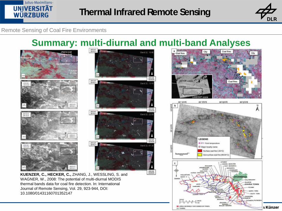
Comparison with High-Res. TIR Data and Ground Truth

• ASTER night-time band 15 (10,95–11,65µm) = comparable to 32

• anomalous clusters extracted from ASTER = orange, MODIS 32 anomalies = grey, hottest zones from ratio image = white. All extracted ASTER hot spots directly on top of or adjacent to MODIS anomalies (slight shift due to rough geolocation?). No clusters outside coalfire area or settled region.

• B: Landsat-5 TM based extraction (manually) Chatterjee (2006) from 1992 data, confirmed in 2003

• C: in-situ mapping result of Michalski (2004)



KUENZER, C., HECKER, C., ZHANG, J., WESSLING, S. and WAGNER, W., 2008: The potential of multi-diurnal MODIS thermal bands data for coal fire detection. In: International Journal of Remote Sensing, Vol. 29, 923-944, DOI: 10.1080/01431160701352147

Summary: multi-diurnal and multi-band Analyses




Conclusion • Weak thermal anomalies cannot be extracted with simple thresholding; but moving window algorithm presented is suitable

• Sensors Landsat, Aster, and MODIS suitable. Thermal MODIS bands allow for multi-diurnal dense observation = optimal thermal monitoring at low cost

• Ratio images of 20/32 à extraction of outstanding hotspots

• Automated thermal anomaly extraction = little bias, no manual “thresholding”, and “twisting until it fits”

• Diurnal approach interesting for forest fire activity monitoring (changes in energy release), industry observation, urban heat pattern analyses, thermal pollution along rivers and coasts, observation of geothermal phenomena, etc.



Further Resources

EARSEL Special Interest Group: Thermal Remote Sensing

• Visit: www.itc.nl/sigtrs


physical principles of remote sensing - earth online

Documents