physically-based motion models for 3d tracking: a...
TRANSCRIPT

Physically-based Motion Models for 3D Tracking: A Convex Formulation
Mathieu SalzmannTTI-Chicago
Raquel UrtasunTTI-Chicago
AbstractIn this paper, we propose a physically-based dynami-
cal model for tracking. Our model relies on Newton’s sec-ond law of motion, which governs any real-world dynami-cal system. As a consequence, it can be generally appliedto very different tracking problems. Furthermore, since theequations describing Newton’s second law are simple linearequalities, they can be incorporated in any tracking frame-work at very little cost. Leveraging this lets us introduce aconvex formulation of 3D tracking from monocular images.We demonstrate the strengths of our approach on varioustypes of motion, such as billiards and acrobatics.
1. IntroductionRecovering the 3D motion of dynamical systems from
monocular images has been an active area of research formany years. To provide robustness to image noise and occlu-sions, as well as to overcome the underlying ambiguities ofthe problem, most practical tracking algorithms exploit mo-tion models. Unfortunately, the existing dynamical modelstypically suffer from one of the two following shortcomings.Either they are very general, but fail to accurately representthe true physical behavior of the system, or they preciselydescribe the observed dynamics, but are very specific and/orhard to optimize. In short, there is a lack of general andpractical motion models.
The motion of any system is governed by laws of physics.Throughout the years, many attempts at encoding these lawsinto dynamical models have been proposed [12, 27, 6]. Re-cent approaches have focused on accurately modeling thebehavior of a single type of motion, e.g., jogging or walk-ing [24, 5]. As a consequence, the resulting methods donot generalize to other motions than those they have beendesigned for. Furthermore, the underlying physical lawsencoded by these models are highly nonlinear, thus yield-ing complex inference problems. Therefore, tracking is per-formed either by simulation, or by minimizing a non-convexobjective function. Both approaches are computationally ex-pensive and may yield suboptimal solutions.
As an alternative to those physically-inspired but im-practical motion models, many tracking algorithms rely on
Figure 1. Billiards shots and acrobatics are examples of the gen-eral tracking scenarios that we address in this paper.
more general Markov dynamical models [19, 7, 11, 8]. Inpractice, these models are typically used to penalize eitheroverly large displacements (i.e., first-order Markov model),or strong variations of velocity (i.e., second-order Markovmodel) between consecutive frames. Higher-order modelscould in principle be employed, but tend to be more sensi-tive to noise, since they provide weaker motion constraints.Unfortunately, while traditional Markov models are not lim-ited to a specific tracking problem, they often do not reflectthe dynamical behavior of real systems.
In this paper, we propose a physics-based dynamicalmodel applicable to general tracking problems. In addi-tion to defining realistic motion constraints, our model hasthe advantage of providing us with an estimate of the exter-nal forces applied to the objects that compose the system.More specifically, we exploit Newton’s second law of mo-tion, which is satisfied by any real-world system. This lawcan be expressed in terms of linear equalities, and thereforecan be incorporated in any tracking system with very littleincrease in inference complexity. By exploiting this prop-erty, we introduce a unified convex formulation of motiontracking for problems as different as bouncing balls, billiardsshots, and human activities (e.g., acrobatics).
We demonstrate the effectiveness of our approach on syn-thetic and real monocular sequences, such as those depictedin Fig. 1, and show that it yields more accurate results thanthose obtained without motion model, as well as with a tra-ditional first-order Markov model. Furthermore, while thesecond-order Markov model can be seen as a special case ofour model, we show that other settings of our approach oftenoutperform this standard regularizer.
1

2. Related Work
Tracking moving, and potentially articulated objects inmonocular video sequences is a poorly-constrained problemdue to, for instance, the presence of noise and occlusions.Existing methods have proposed various solutions to incor-porating additional knowledge about the problem of inter-est to improve 3D reconstruction. While for articulated andnon-rigid pose estimation, much effort has been put into de-signing static constraints [4, 19, 23, 18], here we focus ondynamical models, which are typically used in conjunctionwith the static ones.
A natural way to represent the motion of a dynamicalsystem is to model the underlying physical laws that gov-ern it. Physics-based motion models take their root in com-puter graphics [26, 9, 16, 2, 1]. Following a similar moti-vation, physically-inspired dynamical models were appliedto tracking non-rigid motion [12], as well as human activi-ties [27, 6]. Recently, accurate models have been proposedto represent specific activities, such as jogging or walk-ing [24, 6]. While very well-suited for the particular mo-tion they are designed for, these models do not generalizeto other activities. More importantly, the above-mentionedphysics-based dynamical models typically yield nonlinearconstraints. The resulting methods therefore rely either onnon-convex optimization, or on analysis-by-synthesis, bothof which are computationally expensive and tend to yieldsuboptimal solutions.
As an alternative to physically-inspired models, statisti-cal learning techniques have been proposed to discover thelaws governing the dynamics of a specific system from train-ing data. For human motion tracking, auto-regressive (AR)models have been employed to learn linear relations betweenconsecutive poses [14]. To allow for greater variability inmotion, switching models were introduced [10, 15]. Sincethe AR models are more stable for low-dimensional param-eterizations, they were used in conjunction with linear sub-space models [3, 21]. Following a similar idea of modelingdynamics in a low-dimensional latent space, the GaussianProcess Dynamical Model [25] was applied to human mo-tion tracking [22], thus allowing for nonlinear temporal re-lations. While effective, these models do not generalize be-yond the problem they have been trained on, and thus cannotbe applied to more general tracking scenarios.
Since existing physics-based models yield complex infer-ence problems, and learned models require training data forevery possible motion type, many tracking methods utilizethe simpler, yet more general Markov dynamical models.First-order [7, 11, 8, 17] and second-order [19, 23] Markovmodels are the most popular ones. They are used to eitherbound the range of motion, or limit the variations of velocitybetween consecutive frames in a video sequence. The mainadvantage of these models is their applicability to generaltracking scenarios. Unfortunately, the constraints they pro-
vide are approximate, and as a consequence their predictionsoften tend to be suboptimal.
Here, we take advantage of both physics and Markovmodels. In particular, our approach exploits Newton’s sec-ond law of motion to derive a model that generalizes overthe second-order Markov model by additionally accountingfor the forces applied to the system, thus yielding more flex-ibility. As a consequence, our physically-based dynamicalmodel is simple enough to yield a convex formulation oftracking, while being valid for any real-world tracking sce-nario.
3. A Physically-based Motion Model
In this section, we first review some basic concepts ofkinematics, from which we then derive our model.
3.1. A Review of Kinematics
Newton’s second law of motion is at the core of our dy-namical model. Hence, we first briefly go over its generalformulation, as well as the basic concepts it relies on. Letyi ∈ R3 be the 3D position of the i-th particle belonging toa system of particles. The linear momentum of this singleparticle can be expressed as
pi = mivi , (1)
where vi is the instantaneous velocity of the particle, andmi
is its mass.Newton’s second law of motion states that the accelera-
tion ai produced by a force fi applied to a body of mass mi
has the same direction as fi, and a magnitude directly pro-portional to that of fi and inversely proportional to mi, i.e.,fi = miai. This can be related to the linear momentum bysaying that the instantaneous change in the linear momentumof a particle is equal to the resultant external force acting onthat particle. This can be written as
fi =dpi
dt= miai , (2)
where fi is the sum of all external forces applied to the par-ticle. This formulation relies on the fact that the mass isconstant, i.e., dmi
dt = 0.In practice, the resultant external force fi can arise from
many different types of forces. In our tracking scenarios,we will encounter gravity, friction, collisions, contact andinternal forces arising from the action of human muscles.
3.2. Formulation of our Model
Based on the equations describing Newton’s second lawof motion, we now derive the formulation of our dynamicalmodel. Following physics-based animation techniques, weapproximate the instantaneous velocity at time t using finite
differences. This lets us re-write Eq. 2 as
f ti ≈ mi
(yti − 2yt−1
i + yt−2i
∆t
). (3)
Let us now consider the case of a system of Np par-ticles undergoing motion for Nf time frames. Let yt =[(yt
1)T , · · · , (ytNp
)T ]T be the 3Np dimensional vector con-taining the 3D locations of all particles at time t, and lety = [(y1)T , · · · , (yNf )T ]T be the 3NpNf dimensional vec-tor composed of the 3D locations for the whole sequence. Bytreating all the particles independently, we can impose New-ton’s second law on each particle. This can be expressed as aset of linear constraints in terms of the particles’ coordinatesas
My = fknown + f , (4)
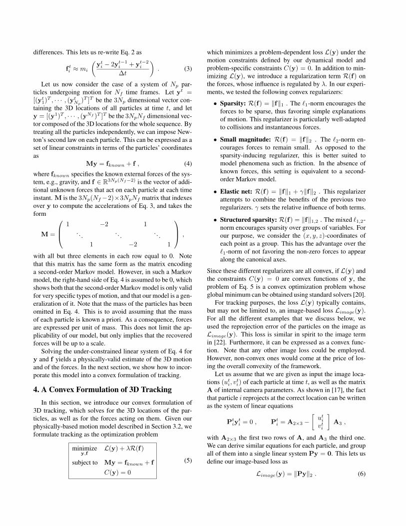
where fknown specifies the known external forces of the sys-tem, e.g., gravity, and f ∈ R3Np(Nf−2) is the vector of addi-tional unknown forces that act on each particle at each timeinstant. M is the 3Np(Nf−2)×3NpNf matrix that indexesover y to compute the accelerations of Eq. 3, and takes theform
M =
1 −2 1. . . . . . . . .
1 −2 1
,
with all but three elements in each row equal to 0. Notethat this matrix has the same form as the matrix encodinga second-order Markov model. However, in such a Markovmodel, the right-hand side of Eq. 4 is assumed to be 0, whichshows both that the second-order Markov model is only validfor very specific types of motion, and that our model is a gen-eralization of it. Note that the mass of the particles has beenomitted in Eq. 4. This is to avoid assuming that the massof each particle is known a priori. As a consequence, forcesare expressed per unit of mass. This does not limit the ap-plicability of our model, but only implies that the recoveredforces will be up to a scale.
Solving the under-constrained linear system of Eq. 4 fory and f yields a physically-valid estimate of the 3D motionand of the forces. In the next section, we show how to incor-porate this model into a convex formulation of tracking.
4. A Convex Formulation of 3D TrackingIn this section, we introduce our convex formulation of
3D tracking, which solves for the 3D locations of the par-ticles, as well as for the forces acting on them. Given ourphysically-based motion model described in Section 3.2, weformulate tracking as the optimization problem
minimizey,f
L(y) + λR(f)
subject to My = fknown + f
C(y) = 0
(5)
which minimizes a problem-dependent loss L(y) under themotion constraints defined by our dynamical model andproblem-specific constraints C(y) = 0. In addition to min-imizing L(y), we introduce a regularization term R(f) onthe forces, whose influence is regulated by λ. In our experi-ments, we tested the following convex regularizers:
• Sparsity: R(f) = ‖f‖1 . The `1-norm encourages theforces to be sparse, thus favoring simple explanationsof motion. This regularizer is particularly well-adaptedto collisions and instantaneous forces.
• Small magnitude: R(f) = ‖f‖2 . The `2-norm en-courages forces to remain small. As opposed to thesparsity-inducing regularizer, this is better suited tomodel phenomena such as friction. In the absence ofknown forces, this setting is equivalent to a second-order Markov model.
• Elastic net: R(f) = ‖f‖1 + γ‖f‖2 . This regularizerattempts to combine the benefits of the previous tworegularizers. γ sets the relative influence of both terms.
• Structured sparsity: R(f) = ‖f‖1,2 . The mixed `1,2-norm encourages sparsity over groups of variables. Forour purpose, we consider the (x, y, z)-coordinates ofeach point as a group. This has the advantage over the`1-norm of not favoring the non-zero forces to appearalong the canonical axes.
Since these different regularizers are all convex, if L(y) andthe constraints C(y) = 0 are convex functions of y, theproblem of Eq. 5 is a convex optimization problem whoseglobal minimum can be obtained using standard solvers [20].
For tracking purposes, the loss L(y) typically contains,but may not be limited to, an image-based loss Limage(y).For all the different examples that we discuss below, weused the reprojection error of the particles on the image asLimage(y). This loss is similar in spirit to the image termin [22]. Furthermore, it can be expressed as a convex func-tion. Note that any other image loss could be employed.However, non-convex ones would come at the price of los-ing the overall convexity of the framework.
Let us assume that we are given as input the image loca-tions (uti, v
ti) of each particle at time t, as well as the matrix
A of internal camera parameters. As shown in [17], the factthat particle i reprojects at the correct location can be writtenas the system of linear equations
Ptiy
ti = 0 , Pt
i = A2×3 −[utivti
]A3 ,
with A2×3 the first two rows of A, and A3 the third one.We can derive similar equations for each particle, and groupall of them into a single linear system Py = 0. This lets usdefine our image-based loss as
Limage(y) = ‖Py‖2 . (6)

10 12.5 16.67 25 50 100
20
25
30
35
40
frame rate [fps]
Mea
n 3D
erro
r [cm
]
0 1 2 3 4 50
10
20
30
40
50
Gaussian noise std
Mea
n 3D
erro
r [cm
]
No model1st orderOurs L1,2
10 12.5 16.67 25 50 100
20
30
40
50
frame rate [fps]
Mea
n 3D
erro
r [cm
]
0 1 2 3 4 5
10
20
30
40
50
60
70
Gaussian noise std
Mea
n 3D
erro
r [cm
]
No model1st orderOurs L1,2
(a) (b) (c) (d)Figure 2. Tracking bouncing balls. (a) Mean 3D error as a function of the framerate for an image Gaussian noise of standard deviation 3.(b) 3D error as a function of the Gaussian noise standard deviation for a framerate of 16.6 fps. (c,d) Similar plots as (a,b) for the case wherethe 2D tracks were lost for up to 0.5 seconds.
2 1 0 1 2 310
20
30
40
50
log10 weight
Mea
n 3D
erro
r [cm
]
1st orderOurs L1Ours L2Ours L1,2
2 1 0 1 2 310
20
30
40
50
log10 weight
Mea
n 3D
erro
r [cm
]
1st orderOurs L1Ours L2Ours L1,2
Figure 3. Influence of model parameters: Mean error as a func-tion of the motion model weights in log scale. (Left) Framerate =100 fps. (Right) Framerate = 10 fps. Note that the best weights forour regularizers are stable across different framerates.
In the case of missing data, the rows of P corresponding tothe missing observations can simply be removed.
The formulation in Eq. 5 is very general. We demon-strate its effectiveness in three different tracking scenarios:3D bouncing balls, billiards and articulated motion. In theremainder of this section, we describe the problem-specificterms C(y) and L(y). Note that other choices are possible.
4.1. 3D Bouncing Balls
We are interested in recovering the 3D motion of one ormore balls bouncing in a room. In this case, gravity playsan important role. Since it has a known and fixed value, wedefine fknown as the concatenation of Np(Nf − 2) copiesof fgravity = mg, where g = [0, 9.81, 0]
Tm/s2, assuming
that the direction of the gravity is in the y-axis of the worldcoordinate system. Furthermore, unknown forces arise fromcollisions with the walls of the room, as well as from colli-sions between the balls. Note that we make no assumptionsabout the number of walls, or about their location and orien-tation.
Without additional image information, recovering the 3Dposition of a single point from its noisy image location isa very ambiguous problem, and a motion model does notsuffice to fully constrain it. Therefore, to be more robust,we create additional image correspondences assuming thatwe are provided with a bounding box around each ball, forexample from a 2D tracker. Knowing the diameter of the3D balls, we can use points sampled on the bounding boxesto create correspondences of the form Pt
i,j(yti + δjy
ti) =
0, where j is an index over the sampled points, and δjyti
represents the corresponding known 3D displacement withrespect to the center of the ball yt
i . Grouping these equationsyields an image-based loss of the form ‖P′y−q‖2, where qcontains the Pt
i,jδjyti . We can thus re-write the optimization
problem of Eq. 5 as
minimizey,f
||P′y − q||2 + λR(f)
subject to My = fknown + f .(7)
4.2. Billiards Balls
In this scenario, we have the additional constraint thatthe balls move on a plane. Here, we assume that we knowthe normal to the plane, which can be obtained from a few3D-to-2D correspondences using a PnP method [13]. Giventhis normal n, we can enforce the trajectory of each ball toremain planar by satisfying
nT(yti − yt−1
i
)= 0 . (8)
With this constraint only, the balls can still move on parallelplanes. To prevent this, we incorporate the additional con-straint
R3y1i = R3y
1i+1 (9)
for Np − 1 balls in the first frame, where R3 is the thirdrow of the rotation matrix transforming camera coordinatesto plane coordinates, typically returned by the PnP method.All these equations can be grouped in a single linear systemof the form By = 0.
The forces acting on billiards balls in motion are verydifferent from the ones acting on 3D bouncing balls. In par-ticular, gravity has no effect, since it is countered by the con-tact forces of the balls on the plane. Therefore, there is noknown forces for this scenario. On the other hand, we expectto have unknown friction forces in addition to the unknowncollision forces. We encode all unknown forces in f . Thislets us re-write the problem of Eq. 5 as
minimizey,f
||P′y − q||2 + λR(f)
subject to My = f
By = 0 .
(10)

(a) (b) (c) (d)Figure 4. Tracking balls in real sequences. (a) Reprojection of the 3D trajectory reconstructed with our approach on the last image of abasketball sequence. (b) Side view of the same trajectory with estimated forces in red. As can be better seen in the video, they match thebounces on the basketball ring. (c,d) Similar plots as (a,b) when tracking several balls in a billiards sequence.
4.3. Articulated Human Motion
Here, we consider the case of human motion tracking andrestrict our image-based loss to the one in Eq. 6. Since re-covering human pose from such poor image information isvery ambiguous, we exploit pose models learned from train-ing data. In particular, we consider both a generative and adiscriminative model.
Discriminative case: We rely on Gaussian processes tolearn a mapping from image observations to 3D poses fromtraining pairs of images and poses [18]. At inference, wefirst apply this mapping to get a prediction yt of the 3D poseat each time t. We then add a term to our loss function L(y)which encourages the reconstruction to remain close to thisprediction. This yields the optimization problem
minimizey,f
||Py||2 + α||y − y||2 + λR(f)
subject to My = fknown + f ,
where y is the vector of all predictions, and α is a constant.
Generative case: We employ a linear subspace modeltrained from 3D poses [19]. At inference, we model eachpose as yt = y0 + Uxt, where y0 is the mean pose, andU is the matrix of eigen-poses. The vector xt contains theweights of the linear combination, and is now treated as theunknown of our problem. The vector of all poses can then bedefined as y = y + Sx, where S is a block-diagonal matrixcontainingNf copies of U, and y and x are the vectors con-catenating the mean pose and the weights xt, respectively.To prevent these weights from becoming overly large, andthus yield meaningless poses, we add a regularization termof the form ‖Λ−1/2xt‖2, where Λ is a diagonal matrix con-taining the eigenvalues of the training data covariance ma-trix. The equations for all frames can be grouped in ‖Lx‖2,where L is the matrix that concatenates Nf replications ofΛ−1/2. We thus re-write our problem as
minimizex,f
||P(y + Sx)||2 + β||Lx||2 + λR(f)
subject to M(y + Sx) = fknown + f .
where β is a scalar.
For both the discriminative and generative cases, depend-ing of the motion of interest, fknown may or may not containgravity. As shown in our experiments, this has very little in-fluence on our results. Note that we do not model the groundplane, which could give us additional constraints.
5. Experimental Evaluation
We now present our results for the different types oftracking problems described in the previous section. Wecompare our reconstructions with those obtained without us-ing any motion model, as well as by employing a standardfirst-order Markov model. To this end, we replaced our dy-namical model in the optimization problems described inSection 4 with a soft penalty on frame-to-frame displace-ments. In addition to different framerates, we ran experi-ments for different levels of additive Gaussian noise in theimage measurements. The weights for the Markov modelregularizer and for our force regularizers were tuned at thehighest framerate and kept unchanged for the rest of the ex-periment. We measure the 3D error in terms of mean point-to-point distance to the ground-truth, averaged over 10 runs.
5.1. 3D Bouncing Balls
To obtain ground-truth data, we implemented a physics-based simulator and computed 10 different sequences, eachseen with a different camera. The bouncing balls are sub-ject to gravity and undergo collisions. We model collisionas an instantaneous force that results in a loss of velocity.This is usually described in terms of the coefficient of resti-tution CR, which relates the velocities before and after theshock. This coefficient varies between CR = 1 (i.e. per-fectly elastic collision) and CR = 0 (i.e. perfectly inelasticcollision, where the bodies stick together after the shock).We use CR = 0.9 for our simulations.
Fig. 2(a,b) depicts the error when tracking 10 bouncingballs as a function of the framerate for a noise of standarddeviation 3, and as a function of the noise for a framerateof 16.67 fps, respectively. The trajectories for these resultswere obtained by solving the problem of Eq. 7. Note thatour approach outperforms the Markov models. As expected,this is particularly true for low framerates, where they are

10 12.5 16.67 25 50 10019
20
21
22
23
24
25
frame rate [fps]
Mea
n 3D
erro
r [cm
]
0 1 2 3 4 50
10
20
30
40
50
Gaussian noise std
Mea
n 3D
erro
r [cm
]
No model1st orderOurs L1,2
10 12.5 16.67 25 50 100
50
100
150
200
250
frame rate [fps]
Mea
n 3D
erro
r [cm
]
0 1 2 3 4 5
50
100
150
200
250
Gaussian noise std
Mea
n 3D
erro
r [cm
]
No model1st orderOurs L1,2
(a) (b) (c) (d)Figure 5. Multiple balls on a plane. (a) Mean 3D error as a function of the framerate for an image Gaussian noise of standard deviation 3.(b) 3D error as a function of the Gaussian noise standard deviation for a framerate of 16.6 fps. (c,d) Similar plots as (a,b) for the case wherethe 2D tracks were lost for up to 0.5 seconds.
1 2 3 40
0.05
0.1
0.15
0.2
log10 weight
Mea
n fri
ctio
n co
ef e
rror
Noise var 0Noise var 1Noise var 3Noise var 5
1 0 1 2 30
0.1
0.2
0.3
0.4
0.5
0.6
log10 weight
Mea
n re
stitu
tion
coef
erro
r
Noise var 0Noise var 1Noise var 3Noise var 5
Figure 6. Recovering physical quantities. (Left) Mean error as afunction of the `1 force penalty weight when recovering the frictioncoefficient. The true coefficient was 0.1. (Right) Similar error forthe coefficient of restitution. The true coefficient was 0.9.
the least accurate. We simulated missing data by removingrandom subsets of consecutive frames for each ball, up to 0.5seconds at a time. Fig. 2(c,d) shows similar plots as beforefor this case. Note that our method remains accurate, whilewithout a motion model the results degrade. The `1,2 normyields the most accurate results among the different regular-izers, thus showing that Markov models are suboptimal here.
Fig. 3 depicts the error as a function of the regularizationweights for the two extreme framerates used in our experi-ments (i.e., 10 and 100 fps). Note that the best weights forour regularizers remain more stable across different framer-ates than for the first-order Markov model. This suggeststhat our model is less sensitive to this parameter, and henceeasier to apply in real scenarios.
We also tracked a basketball shot in a YouTube video.The 2D tracks and bounding boxes were obtained by a sim-ple template-matching method that maximizes the normal-ized cross-correlation between a template defined in the firstimage and the following images of the sequence. The re-projection on an input image of the 3D trajectory recon-structed using our approach with the `1 regularizer is shownin Fig. 4(a), and its side view in blue in Fig. 4(b). Note thatthe estimated forces, depicted in red, occur when the balltouches the ring, and thus correspond to those we expect.
5.2. Billiards Balls
We implemented a simulator to generate balls movingon a plane, thus mimicking billiards. We employed thesame collision model as before and simulated friction asffriction = −µ‖fn‖v/‖v‖, where µ is the friction coeffi-
cient, and fn is the normal force. In contrast to the bouncingballs, we do not model gravity. We computed 10 differentsequences, seen from different viewpoints, and simulatedmissing data as before. 3D tracking was performed by solv-ing the optimization problem of Eq. 10. Fig. 5 depicts theerrors obtained for the case of 5 moving balls colliding witheach other and with the table edges. Note that the `1,2 normyields more accurate results than the Markov model and theother regularizers. With missing data, it also significantlyoutperforms the results obtained without motion model.
Fig. 4(c,d) depicts our tracking results on a billiards videofrom YouTube. The 2D tracks were obtained in a similarmanner as in the basketball case. The top view in Fig. 4(d)shows that the trajectory recovered by our approach with an`1 regularizer matches what we observe in the images, andthat the estimated forces correspond to those we expect.
Our model can also be used to estimate physical con-stants, such as the friction and restitution coefficients, fromthe reconstructed forces and trajectories. For the friction co-efficient, we post-processed the estimated forces by discard-ing the large ones. We then recovered µ by least-squaresfitting based on the equation of friction, using gravity as thenormal force. As shown in Fig. 6(left), this results in accu-rate estimates. Fig. 6(right) depicts the error when estimat-ing the restitution coefficient. In this case, CR was obtainedfrom the velocities before and after the collisions, whichwere detected by finding the large forces.
5.3. Human Motion
To address the problem of tracking people performingdifferent activities, we exploited the publicly available CMUmotion capture dataset1 and tested our approach on threedifferent activities: jumping, jogging and acrobatics (i.e.,a front handspring). The 2D tracks were obtained by pro-jecting the 3D data using a known camera. Gaussian noisewas added to these image locations with standard deviationranging from 0 to 10. As mentioned in Section 4, since theproblem of human body tracking from 2D correspondencesis too ambiguous, we augmented our motion model, as wellas the baselines, with pose models. We used the poses froma subset of the data as training examples, and the remaining
1http://mocap.cs.cmu.edu/

1.2 1.4 1.6 1.8 2
5
6
7
8
9
log10 frame rate [fps]
Mea
n 3D
erro
r [cm
]
GPNo model1st orderOurs L1,2
0 2 4 6 8 10
4
5
6
7
8
9
10
Gaussian noise std
Mea
n 3D
erro
r [cm
]
1.2 1.4 1.6 1.8 2
5
6
7
8
9
log10 frame rate [fps]
Mea
n 3D
erro
r [cm
]
GPNo model1st orderOurs L1,2
0 2 4 6 8 10
4
5
6
7
8
9
10
Gaussian noise std
Mea
n 3D
erro
r [cm
]
(a) (b) (c) (d)Figure 7. Tracking a human jumping with a discriminative model. (a) Mean 3D error as a function of the framerate for an image Gaussiannoise of standard deviation 6. (b) 3D error as a function of the Gaussian noise standard deviation for a framerate of 20 fps. (c,d) Similarplots as (a,b) when the gravity is not explicitly encoded in the known forces. Note that this does not significantly affect our results.
1.2 1.4 1.6 1.8 24
4.2
4.4
4.6
4.8
5
5.2
log10 frame rate [fps]
Mea
n 3D
erro
r [cm
]
No model1st orderOurs L1,2
0 2 4 6 8 10
3.5
4
4.5
5
5.5
Gaussian noise std
Mea
n 3D
erro
r [cm
]
1.2 1.4 1.6 1.8 24
6
8
10
12
log10 frame rate [fps]
Mea
n 3D
erro
r [cm
]
No model1st orderOurs L1,2
0 2 4 6 8 10
456789
10
Gaussian noise std
Mea
n 3D
erro
r [cm
]
(a) (b) (c) (d)Figure 8. Tracking a human jumping with a linear subspace model. (a) Mean 3D error as a function of the framerate for an imageGaussian noise of standard deviation 6 and with missing 2D tracks. (b) 3D error as a function of the Gaussian noise standard deviation for aframerate of 20 fps and with missing 2D tracks. (c,d) Similar plots as (a,b) in the case of full occlusions.
sequences as test data. To simulate missing data (i.e., losttracks), we removed correspondences in consecutive frames.We also simulated full occlusions by removing all the trackssimultaneously for several frames.
Figs. 7 and 8 summarize our results for a jumping motionwhen using a Gaussian process mapping and a linear sub-space model, respectively. Fig. 7(a,b) shows the 3D errors asa function of the framerate for a Gaussian noise of standarddeviation 6, and as a function of the noise for a framerateof 20 fps. Fig. 7(c,d) shows similar plots when the gravitywas not explicitly encoded in the known forces. Note thatthis has little influence on our results. Fig. 8 depicts the er-rors in the presence of missing 2D measurements and fullocclusions. As can be observed from the plots, our approachis robust to these phenomena. In Fig. 9, we show the er-rors obtained for a jogging motion with a Gaussian processmapping. As before, the explicit use of gravity has little in-fluence on our results. Fig. 10 depicts the errors obtained forthe front handspring motion when relying on a linear sub-space model. Similarly as for the jumping motion, missingdata and full occlusions do not significantly affect our recon-structions. Note that, in all these scenarios, our model con-sistently outperforms the first-order Markov model. Further-more, in most experiments, the `1,2 norm gives the best per-formance, with the `2 norm being second best. This showsthat other settings of our approach often outperform the tra-ditional special case of second-order Markov models. Fi-nally, in Figs. 1 and 11, we show examples of reconstruc-tions obtained with an image noise of standard deviation 4.
6. Conclusion and Future WorkIn this paper, we have presented a physics-based dynam-
ical model that combines the advantages of being generallyapplicable and easy to optimize. By exploiting our model,we have introduced a convex formulation of 3D tracking thatnot only recovers 3D trajectories, but also yields an estimateof the forces applied to the system. Finally, we have shownthat our approach is general enough to handle very differenttracking scenarios, and that it outperforms the standard first-and second-order Markov models, the latter being a specialcase of our model. While we have considered the problem of3D motion tracking, our dynamical model could also be ap-plied to other problems, such as camera motion estimation,or post-processing of motion capture data. In the future, weplan to study other physical constraints, such as balance, toimprove 3D reconstruction.
References[1] D. Baraff. Analytical methods for dynamic simulation of non-
penetrating rigid bodies. ACM SIGGRAPH, 1989.[2] R. Barzel and A. H. Barr. A modeling system based on dy-
namic constraints. ACM SIGGRAPH, 1988.[3] A. Bissacco. Modeling and Learning Contact Dynamics in
Human Motion. CVPR, 2005.[4] V. Blanz and T. Vetter. A Morphable Model for the Synthesis
of 3D Faces. ACM SIGGRAPH, 1999.[5] M. Brubaker, D. Fleet, and A. Hertzmann. Physics-based
Person Tracking Using the Anthropomorphic Walker. IJCV,87(1), 2010.

1.2 1.4 1.6 1.8 2
5
6
7
8
9
10
log10 frame rate [fps]
Mea
n 3D
erro
r [cm
]
GPNo model1st orderOurs L1,2
0 2 4 6 8 10
5
6
7
8
9
10
Gaussian noise std
Mea
n 3D
erro
r [cm
]
1.2 1.4 1.6 1.8 2
5
6
7
8
9
10
log10 frame rate [fps]
Mea
n 3D
erro
r [cm
]
GPNo model1st orderOurs L1,2
0 2 4 6 8 104
5
6
7
8
9
10
Gaussian noise std
Mea
n 3D
erro
r [cm
]
(a) (b) (c) (d)Figure 9. Tracking a human jogging. (a) Mean 3D error as a function of the framerate for an image Gaussian noise of standard deviation6. (b) 3D error as a function of the Gaussian noise standard deviation for a framerate of 20 fps. (c,d) Similar plots as (a,b) when the gravityis not encoded in the known forces. Note that this does not significantly affect the results of our approach.
1.2 1.4 1.6 1.8 25.8
6
6.2
6.4
6.6
6.8
7
log10 frame rate [fps]
Mea
n 3D
erro
r [cm
]
No model1st orderOurs L1,2
0 2 4 6 8 10
6
6.5
7
7.5
Gaussian noise std
Mea
n 3D
erro
r [cm
]
1.2 1.4 1.6 1.8 2
8
10
12
14
16
log10 frame rate [fps]
Mea
n 3D
erro
r [cm
]
No model1st orderOurs L1,2
0 2 4 6 8 10
8
10
12
14
Gaussian noise std
Mea
n 3D
erro
r [cm
]
(a) (b) (c) (d)Figure 10. Tracking a human performing a front handspring. (a) Mean 3D error as a function of the framerate for an image Gaussiannoise of standard deviation 6 and with missing 2D tracks. (b) 3D error as a function of the Gaussian noise standard deviation for a framerateof 20 fps and with missing 2D tracks. (c,d) Similar plots as (a,b) in the case of full occlusions.
Figure 11. Tracking human motion. Reconstructions of a jumpingand a jogging sequence with an image noise of variance 4.
[6] M. Brubaker, L. Sigal, and D. Fleet. Estimating Contact Dy-namics. ICCV, 2009.
[7] K. Choo and D. Fleet. People Tracking Using Hybrid MonteCarlo Filtering. ICCV, 2001.
[8] J. Deutscher and I. Reid. Articulated Body Motion Captureby Stochastic Search. IJCV, 61(2), 2004.
[9] J. K. Hodgins, W. L. Wooten, D. C. Brogan, and J. F. O’Brien.Animating Human Athletics. ACM SIGGRAPH, 1995.
[10] M. Isard and A. Blake. A mixed-state Condensation trackerwith automatic model-switching. ICCV, 1998.
[11] A. Jepson, D. J. Fleet, and T. El-Maraghi. Robust On-LineAppearance Models for Vision Tracking. PAMI, 25(10),2003.
[12] D. Metaxas and D. Terzopoulos. Shape and Nonrigid MotionEstimation Through Physics-Based Synthesis. PAMI, 15(6),1993.
[13] F. Moreno-Noguer, V. Lepetit, and P. Fua. Accurate Non-Iterative o(n) Solution to the Pnp Problem. ICCV, 2007.
[14] B. North, A. Blake, M. Isard, and J. Rittscher. Learning andclassification of complex dynamics. PAMI, 25(9), 2000.
[15] V. Pavlovic, J. Rehg, and J. Maccormick. Learning switchinglinear models of human motion. NIPS, 2000.
[16] Z. Popovic and A. Witkin. Physically Based Motion Trans-formation. ACM SIGGRAPH, 1999.
[17] M. Salzmann, V. Lepetit, and P. Fua. Deformable SurfaceTracking Ambiguities. CVPR, 2007.
[18] M. Salzmann and R. Urtasun. Combining discriminative andgenerative methods for 3d deformable surface and articulatedpose reconstruction. CVPR, 2010.
[19] H. Sidenbladh, M. J. Black, and D. J. Fleet. Stochastic Track-ing of 3D Human Figures Using 2D Image Motion. ECCV,2000.
[20] J. Sturm. Using SeDuMi 1.02, a MATLAB toolbox for opti-mization over symmetric cones, 1999.
[21] L. Torresani, A. Hertzmann, and C. Bregler. NonrigidStructure-From-Motion: Estimating Shape and Motion WithHierarchical Priors. PAMI, 30(5), 2008.
[22] R. Urtasun, D. Fleet, and P. Fua. 3D People Tracking WithGaussian Process Dynamical Models. CVPR, 2006.
[23] R. Urtasun, D. Fleet, A. Hertzman, and P. Fua. Priors forPeople Tracking from Small Training Sets. ICCV, 2005.
[24] M. Vondrak, L. Sigal, and O. C. Jenkins. Physical Simulationfor Probabilistic Motion Tracking. CVPR, 2008.
[25] J. Wang, D. Fleet, and A. Hertzmann. Gaussian Process Dy-namical Models for Human Motion. PAMI, 30(2), 2008.
[26] A. Witkin and M. Kass. Spacetime Constraints. ACM SIG-GRAPH, 1988.
[27] C. Wren and A. Pentland. Dynamic Models of Human Mo-tion. FG, 1998.