physics 1502: lecture 23 today’s agenda
DESCRIPTION
Announcements: RL - RV - RLC circuits Homework 06: due next Wednesday … Maxwell’s equations / AC current. Physics 1502: Lecture 23 Today’s Agenda. X X X X X X X X X. Induction. Self-Inductance, RL Circuits. long solenoid. Energy and energy density. In series (like resistors). a. - PowerPoint PPT PresentationTRANSCRIPT

Physics 1502: Lecture 23Today’s Agenda
• Announcements:– RL - RV - RLC circuits
• Homework 06: due next Wednesday …Homework 06: due next Wednesday …
• Maxwell’s equations / AC current

InductionSelf-Inductance, RL Circuits
X X X X X X X X X
RI
ε
a
b
L
I
long solenoid
Energy and energy density

Inductors in Series and Parallel• In series (like resistors) a
b
L2
L1
a
b
Leq
And:
a
b
L2L1
a
b
Leq
• In parallel (like resistors)
And finally:

Summary of E&M• J. C. Maxwell (~1860) summarized all of the work on
electric and magnetic fields into four equations, all of which you now know.
• However, he realized that the equations of electricity & magnetism as then known (and now known by you) have an inconsistency related to the conservation of charge!
I don’t expect you to see that these equations are inconsistent with conservation of charge, but you should see a lack of symmetry here!
Gauss’ Law
Gauss’ LawFor Magnetism
Faraday’s Law
Ampere’s Law

Ampere’s Law is the Culprit!• Gauss’ Law:
• Symmetry: both E and B obey the same kind of equation (the difference is that magnetic charge does not exist!)
• Ampere’s Law and Faraday’s Law:
• If Ampere’s Law were correct, the right hand side of Faraday’s Law should be equal to zero -- since no magnetic current.
• Therefore(?), maybe there is a problem with Ampere’s Law.
• In fact, Maxwell proposes a modification of Ampere’s Law by adding another term (the “displacement” current) to the right hand side of the equation! ie
!

Displacement current
Remember:
E
Iin Iout
changing electric flux

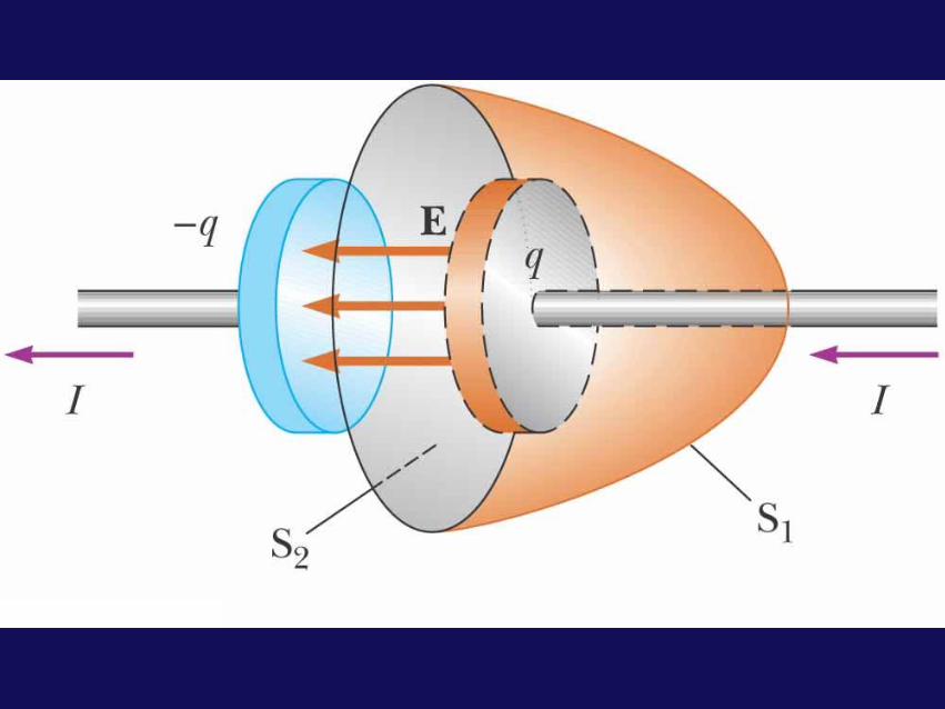

Maxwell’s Displacement Current
• Can we understand why this “displacement current” has the form it does?
• Consider applying Ampere’s Law to the current shown in the diagram.
• If the surface is chosen as 1, 2 or 4, the enclosed current = I• If the surface is chosen as 3, the enclosed current = 0! (ie there is no current between the plates of the capacitor)
Big Idea: The Electric field between the plates changes in time. “displacement current” ID = ε0 (dE/dt) = the real current I in the wire.
circuit

Maxwell’s Equations• These equations describe all of Electricity and
Magnetism.
• They are consistent with modern ideas such as relativity.
• They even describe light

LC
ε
R
φ
φ
φ
imR
imL
imC
εm

Power ProductionAn Application of Faraday’s Law
• You all know that we produce power from many sources. For example, hydroelectric power is somehow connected to the release of water from a dam. How does that work?
• Let’s start by applying Faraday’s Law to the following configuration:
N
S
N
S
Side View
N
S
End View

Power ProductionAn Application of Faraday’s Law
• Apply Faraday’s Law

Power ProductionAn Application of Faraday’s Law
• A design schematic
Water

RLC - Circuits
• Add resistance to circuit:LC
ε
R
• Qualitatively: Oscillations created by L and C are damped (energy dissipation!)
• Compare to damped oscillations in classical mechanics:

AC Circuits - Intro
• However, any real attempt to construct a LC circuit must account for the resistance of the inductor. This resistance will cause oscillations to damp out.
• Question: Is there any way to modify the circuit above to sustain the oscillations without damping?
• Answer: Yes, if we can supply energy at the rate the resistor dissipates it! How? A sinusoidally varying emf (AC generator) will sustain sinusoidal current oscillations!
• Last time we discovered that a LC circuit was a natural oscillator.
LC+ +
- -
R

AC CircuitsSeries LCR• Statement of problem:
Given ε = εmsint , find i(t).
Everything else will follow.
• Procedure: start with loop equation?
• We could solve this equation in the same manner we did for the LCR damped circuit. Rather than slog through the algebra, we will take a different approach which uses phasors.
LC
ε
R

εR Circuit• Before introducing phasors, per se, begin by considering
simple circuits with one element (R,C, or L) in addition to the driving emf.
• Begin with R: Loop eqn gives:
Voltage across R in phase with current through R
εiR
R
Note: this is always, always, true… always.
0
V R
tx
εm
εm
0
0 t
iRεm / R
εm / R
0
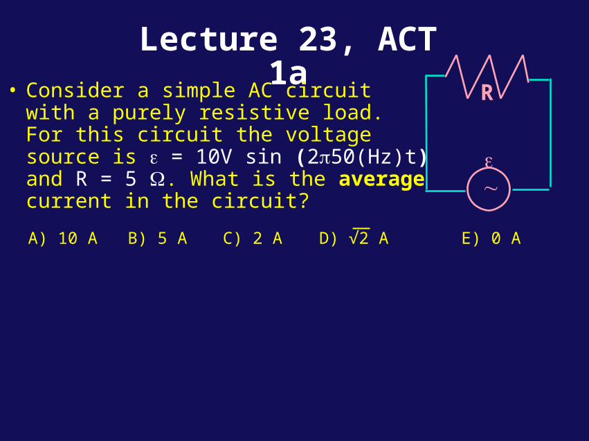
Lecture 23, ACT 1a
• Consider a simple AC circuit with a purely resistive load. For this circuit the voltage source is ε = 10V sin (250(Hz)t) and R = 5 . What is the average current in the circuit?
ε
R
A) 10 A B) 5 A C) 2 A D) √2 A E) 0 A

Chapter 28, ACT 1b• Consider a simple AC circuit with a
purely resistive load. For this circuit the voltage source is ε = 10V sin (250(Hz)t) and R = 5 . What is the average power in the circuit?
ε
R
A) 0 W B) 20 W C) 10 W D) 10 √2 W
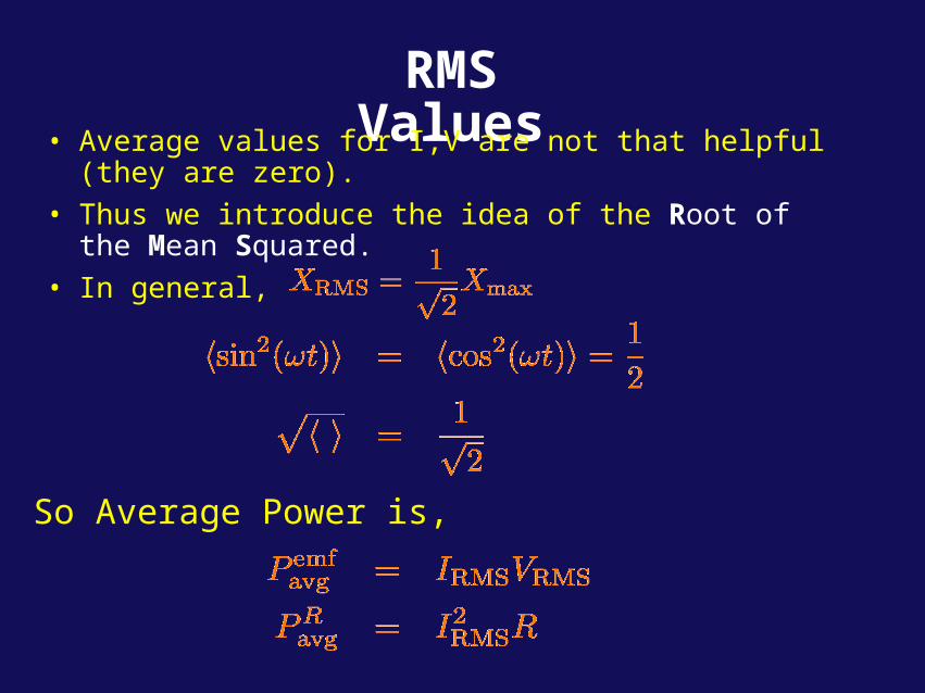
RMS Values• Average values for I,V are not that helpful (they are zero).
• Thus we introduce the idea of the Root of the Mean Squared.
• In general,
So Average Power is,
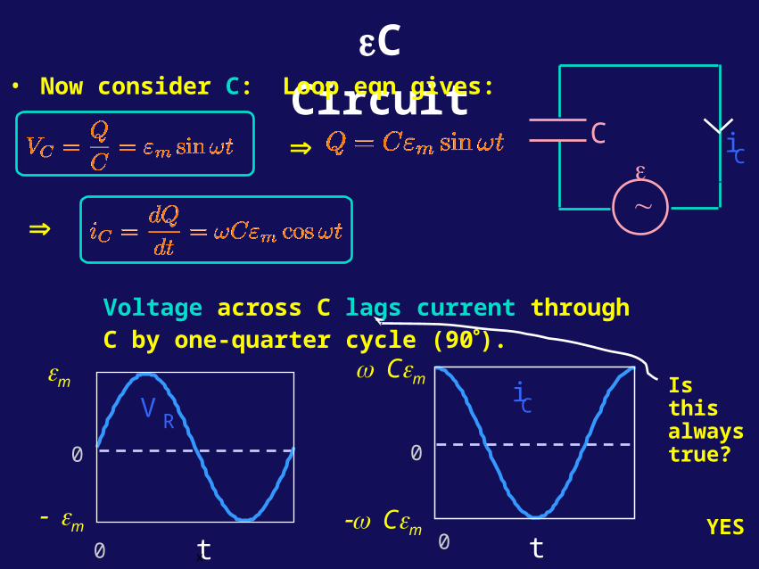
εC Circuit• Now consider C: Loop eqn gives:
ε
C iC
Voltage across C lags current through C by one-quarter cycle (90).
Is this always true?
YES
0
V R
tx
εm
εm
0
t
0
iC
0
Cεm
Cεm
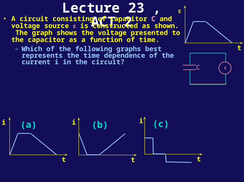
Lecture 23 , ACT 2• A circuit consisting of capacitor C and voltage
source ε is constructed as shown. The graph shows the voltage presented to the capacitor as a function of time. – Which of the following graphs best represents
the time dependence of the current i in the circuit?
(a) (b) (c)i
t
i
t t
i
ε
t
εC
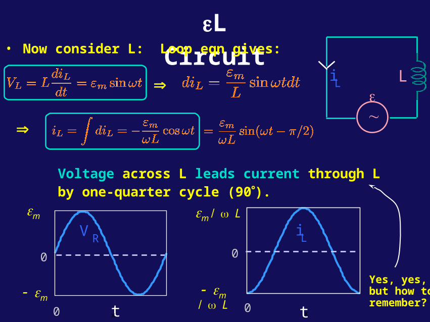
εL Circuit• Now consider L: Loop eqn gives:
Voltage across L leads current through L by one-quarter cycle (90).
ε
LiL
Yes, yes, but how to remember?
0
V R
tx
εm
εm
0
t
iL
x
εm L
εm L 0
0
Phasors
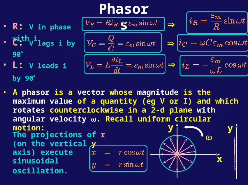
• A phasor is a vector whose magnitude is the maximum value of a quantity (eg V or I) and which rotates counterclockwise in a 2-d plane with angular velocity . Recall uniform circular motion:
The projections of r (on the vertical y axis) execute sinusoidal oscillation.
• R: V in phase with i
• C: V lags i by 90
• L: V leads i by 90
x
y y

Phasors for L,C,Ri
t
V
R
i
t
VL
i
t
VC
t
iV
R
0
VC
0
i
i
0
VL
2
Suppose:

Lecture 23, ACT 3• A series LCR circuit driven by emf ε = ε0sint
produces a current i=imsin(t-). The phasor diagram for the current at t=0 is shown to the right.– At which of the following times is VC, the
magnitude of the voltage across the capacitor, a maximum?
LC
∼ε
R
i
t=0
(a) (b) (c)i
t=0
i
t=tb
i
t=tc

Series LCR
AC Circuit• Consider the circuit shown here: the loop equation gives:
• Here all unknowns, (im,) , must be found from the loop eqn; the initial conditions have been taken care of by taking the emf to be: εεm sint.
• To solve this problem graphically, first write down expressions for the voltages across R,C, and L and then plot the appropriate phasor diagram.
LC
ε
R
• Assume a solution of the form:

Phasors: LCR
• Assume:
• From these equations, we can draw the phasor diagram to the right.
φ
φ
φ
imR
imL
imC
εm
LC
ε
R
• This picture corresponds to a snapshot at t=0. The projections of these phasors along the vertical axis are the actual values of the voltages at the given time.
• Given:

Phasors: LCR
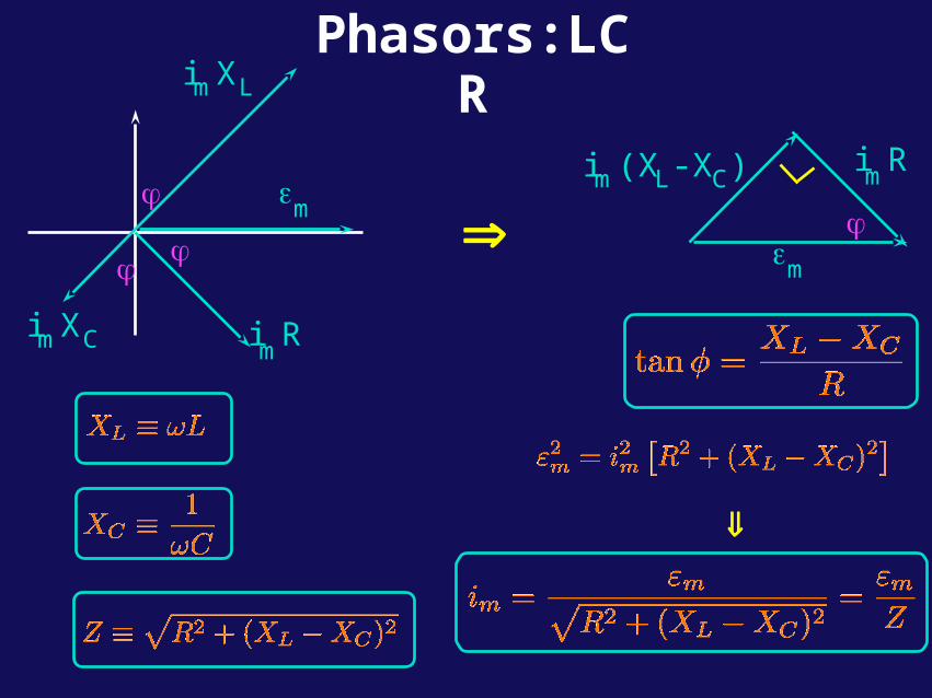
• The phasor diagram has been relabeled in terms of the reactances defined from:
φ
φ
φ
imR
εm
imXC
imXL
LC
ε
R
The unknowns (im,) can now be solved for graphically since the vector sum of the voltages VL + VC + VR must sum to the driving emfε.
Phasors:LCR
imR
εm
φ
im(XL-X C)
φφ
φ
imR
εm
imXC
imXL

Phasors:Tips• This phasor diagram was drawn as a snapshot of time t=0 with the voltages being given as the projections along the y-axis.
φφ
φ
imR
εm
imXC
imXLy
x
imR
imXL
imXC
εm
“Full Phasor Diagram”
From this diagram, we can also create a triangle which allows us to calculate the impedance Z:
• Sometimes, in working problems, it is easier to draw the diagram at a time when the current is along the x-axis (when i=0).
“ Impedance Triangle”
Z
|
R
| XL-XC |