1

Physics of Acoustic Radiation from Jet Engine Inlets

Christopher K. W. Tam1, Sarah A. Parrish

2, Edmane Envia

3 and Eugene W. Chien

4

1,2Florida State University, Tallahassee, FL 32306-4510

3NASA Glenn Research Center, Cleveland, OH 44135

4Goodrich Aerostructures Group, Chula Vista, CA 91910

Numerical simulations of acoustic radiation from a jet engine inlet are performed using

advanced computational aeroacoustics (CAA) algorithms and high-quality numerical

boundary treatments. As a model of modern commercial jet engine inlets, the inlet geometry of

the NASA Source Diagnostic Test (SDT) is used. Fan noise consists of tones and broadband

sound. This investigation considers the radiation of tones associated with upstream

propagating duct modes. The primary objective is to identify the dominant physical processes

that determine the directivity of the radiated sound. Two such processes have been identified.

They are acoustic diffraction and refraction. Diffraction is the natural tendency for an acoustic

wave to follow a curved solid surface as it propagates. Refraction is the turning of the direction

of propagation of sound waves by mean flow gradients. Parametric studies on the changes in

the directivity of radiated sound due to variations in forward flight Mach number and duct

mode frequency, azimuthal mode number, and radial mode number are carried out. It is

found there is a significant difference in directivity for the radiation of the same duct mode

from an engine inlet when operating in static condition and in forward flight. It will be shown

that the large change in directivity is the result of the combined effects of diffraction and

refraction.

1. Introduction

Acoustic radiation from jet engine inlets has been studied experimentally

1-9, analytically

10-13 and

computationally14-26

by a number of investigators in the past. These studies provide a variety of useful and

interesting information. They also provide prediction capabilities and methods. It is known that sound radiated out

of an engine inlet consists of both broadband noise and tones. Broadband fan noise is random and chaotic and is best

studied statistically. Tones, on the other hand, which are generated by the fan rotating at high speeds and by the

cutting of the rotor wake by the stator blades, are highly organized and propagate coherently. In the inlet duct, tones

propagate as duct modes. Because duct modes are coherent propagating entities, they are readily open to analysis

and numerical simulation. Their propagating characteristics are also easy to understand. Duct mode propagation

from the fan face to the far field is the subject of the present investigation.

It is our belief that the mechanisms that influence the radiation of duct modes operate independent of the

engine inlet geometry; the geometry of the engine inlet does, however, alter the relative importance of the various

mechanisms. For this reason, this study uses primarily the inlet geometry of the NASA Source Diagnostic Test

(SDT) fan, which has internal fan duct diameter of approximately 22 inches at the fan face. The fan has 22 blades.

The inlet geometry of the SDT fan is typical of most modern jet engines.

There is significant complexity in the duct mode radiation processes. To illustrate this point, consider the

radiation patterns associated with the NASA SDT fan inlet in Figs. 1 and 2. The flow Mach number at the fan face is

the same for both cases: Mfan = 0.4. The duct mode radiating out of the inlet is also the same in each case and is

defined with azimuthal mode number m = 22, radial mode number n = 1, and frequency f = 6400 Hz. Fig. 1 shows

1 Robert O. Lawton Distinguished Professor, Department of Mathematics, AIAA Fellow.

2 Research Associate, Department of Mathematics.

3 Research Aerospace Engineer, Acoustics Branch, AIAA Associate Fellow.

4 Staff Engineer, Acoustics

https://ntrs.nasa.gov/search.jsp?R=20130000433 2018-07-30T03:03:48+00:00Z

2

the pressure contour pattern for the engine at static condition, i.e., no forward flight. Fig. 2 shows the pressure

contour pattern when the engine is moving with forward flight Mach number 0.2. It is obvious that the dominant

directions of radiation in the two cases are substantially different. But why are they so different for such a low flight

Mach number? Currently, a valid explanation does not appear to be available in the open literature.

Figure 1. Computed pressure contour pattern of an m = 22, n = 1 duct mode at 6400 Hz

radiating out of the SDT fan inlet. Mfan = 0.4, Mflight = 0.0 (static condition).

Figure 2. Computed pressure contour pattern of an m = 22, n = 1 duct mode at 6400 Hz

radiating out of the SDT fan inlet. Mfan = 0.4, Mflight = 0.2.

Thus, in spite of past studies, there seems to be a need for further effort in the investigation of the flow

physics that controls and influences the acoustic radiation processes. This is the purpose of the present investigation.

To accomplish this goal, numerical simulation using advanced computational aeroacoustics (CAA) methods is used.

We would like to point out that, for the stated purpose, numerical simulation has some significant advantages over

an experimental investigation. This does not mean that experiments are unimportant. Actually, they are absolutely

necessary for validation and other purposes. A few of these advantages are listed below.

3

1. In a numerical simulation, there is full access to space and time data inside and outside an engine inlet. They

include both the mean flow and acoustic disturbances. These types of data are needed in order to understand the

physical processes involved in the radiation of a duct mode. In principle, these quantities can also be measured

experimentally. But to do so would require an extraordinary effort; therefore, it has never been done.

2. Computationally, the amount of effort required to simulate engine inlet radiation with and without forward flight

is about the same. Experimentally, studying forward flight effect in a laboratory would require the use of a wind

tunnel, which introduces background wind tunnel noise and possible extraneous tones from the facility.

Complications also arise from wall reflection, if a closed wind tunnel is used, and from shear layer correction, if

an open wind tunnel is used.

3. Numerical simulation allows an easy study of the radiation of an individual duct mode. A parametric study of the

variation of mode frequency and azimuthal and radial mode numbers can easily be carried out. Experimentally,

generating a single duct mode is no trivial matter. Usually, the measured pressure signal contains a multitude of

modes. Unscrambling the measured pressure data in order to recover individual mode information is not an easy

task.

In this paper, it is our intent to show that duct mode radiation from a jet engine inlet is greatly influenced

by the effects of diffraction and refraction. Here, diffraction refers to the inherent characteristic of a duct mode to

follow and remain attached to the wall of the engine casing as it propagates and eventually radiates away. Refraction

is the turning of the direction of propagation of a duct mode by mean flow gradients. The degree of influence of

these two effects is, however, highly dependent on fan face Mach number, Mfan, forward flight Mach number, Mflight,

azimuthal and radial mode numbers, (m,n), and frequency, f. The sum of all the individual effects ultimately

determines the dominant direction of radiation for a duct mode. The present investigation focuses on finding the

dependence of the diffraction and refraction effects on each of the above parameters. Reporting and explaining these

results forms the main body of this paper. In addition, we will document the CAA methods and algorithms used, as

they may be of interest to other investigators. To assure that our simulations are accurate, we have performed

validation tests by comparing the computed directivity with experimental measurements.

The rest of the paper is as follows: Section 2 discusses the computational grid, computational model and

algorithm, as well as various types of boundary conditions used in the present numerical simulations. Section 3

reports the results of a series of computer code validation tests. Directivity data from a JT15D engine experiment1,2

is used for comparison. Section 4 presents computed mean flow data, both with and without forward flight, for the

NASA SDT engine inlet. Acoustic results are reported in Section 5. They include a detailed study of the effects of

diffraction and refraction. An explanation for the large impact of forward flight on the direction of duct mode

radiation is presented. A parametric study showing the effects of forward flight Mach number, duct mode frequency,

and azimuthal and radial mode numbers on the radiation pressure contour pattern and directivity has been carried

out. The results of this parametric study are reported in Section 6. The impact of diffraction and refraction effects on

these results is explained. Section 7 gives a summary and conclusion of this work.

2. Computational Model, Grid Design, and Computational Algorithm

In this section, information on the computational domain, computational model, grid design and

computational algorithm used in the present numerical simulation of jet engine inlet radiation is provided.

2.1 Grid design

Fig. 3 shows the computational domain in physical space. The engine inlet is at the lower-right corner. The

internal diameter, D, of the casing at the fan face is used as the length scale. For the NASA STD fan, D is

approximately 22 inches. There are twenty-two fan blades. The computational domain extends five diameters (5D)

in front of the fan face and four diameters (4D) in the sideline direction. This is the size of the domain used for near

field pressure contour pattern computation. For validation directivity computations, the domain is extended further

to the left by another 5D. To generate a body-fitted grid, a conformal mapping method is used27

. The engine casing

and hub is first extended by symmetry about the vertical line passing through the fan face as shown in Fig. 4.

4

Figure 3. Computational domain for near field pressure contour pattern computations.

Doublets are placed along the centerlines of the three bodies in Fig. 4. A large set of enforcement points on

the surface of the bodies is selected. The strengths of the doublets are then chosen so the enforcement points are

mapped onto three parallel slits in the computational plane as shown in Fig. 5. Because the number of enforcement

points is much higher than the number of doublets, the number of linear algebraic equations derived from mapping

to the slits condition is far higher than the number of unknowns. It is an over-determined system. Such a system can,

however, be solved by a mean-least-squared method known as the method of normal matrix. Details of the

conformal mapping method are provided in Ref. [27].

Figure 4. Locations of doublets and enforcement points for conformal mapping of the engine inlet into 3 slits.

5

Figure 5. Mapping of engine inlet into three slits in the computational domain.

In the mapped plane, i.e., the computation plane or the plane, the inlet consists of three slits. A

Cartesian grid can easily be fitted into the three-slits geometry in the computational domain, as shown in Fig. 6.

Because of axisymmetry, only the top half of the inlet needs be considered. A multiple-size grid is used to ensure

accuracy and efficiency. The finest grid is used around the walls of the casing and the hub, as shown in Fig. 6. In

moving outward from these finest regions, three grid-size changes occur, each increasing the grid size by a factor of

two. The result is a total of four grid sizes, where the grid size of the coarsest region is eight times that of the finest

region. This grid arrangement is adopted in anticipation of using the multi-size-mesh and multi-time-step DRP

scheme28

as the computational algorithm.

Figure 6. Multi-size Cartesian grid in the computational plane or the plane.

Figure 7. Elliptic coordinate lines form a body-fitted grid around a slit.

6

In the computational domain, both the casing and the hub are mapped into slits. A Cartesian grid would

provide adequate resolution everywhere except at the tip of the slit. To improve resolution near the tips of the slits,

an elliptic grid ( coordinates), which forms a body-fitted grid to a slit, is introduced (see Fig. 7). A lens-

shaped portion of the elliptic grid, as shown in Fig. 8, is included in the computation. The Cartesian grid

computation ends at the boundary of the rectangular box shown in Fig. 8. The computation in the elliptic grid is

confined to the lens-shaped region in this figure. In the overlapping region, data are transferred by interpolation from

one grid to the other, typical of the overset grid method29

. In the physical plane, the grid design around the casing

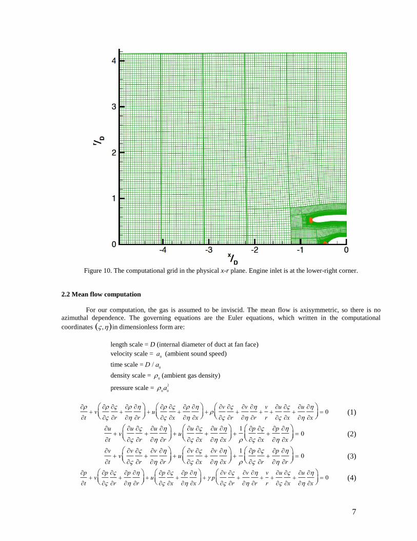
and the hub is shown in Fig. 9. The computational grid in the physical plane is displayed in Fig. 10. Note in Figs. 9

and 10, the grids have been coarsened for illustrative purposes.

Figure 8. A lens-shaped region of the elliptic grid of Fig. 7 is used

to improve resolution at the tip of a slit.

Figure 9. Enlarged grid design in the computational and the physical planes.

7

Figure 10. The computational grid in the physical x-r plane. Engine inlet is at the lower-right corner.

2.2 Mean flow computation

For our computation, the gas is assumed to be inviscid. The mean flow is axisymmetric, so there is no

azimuthal dependence. The governing equations are the Euler equations, which written in the computational

coordinates , in dimensionless form are:

length scale = D (internal diameter of duct at fan face)

velocity scale = a0

(ambient sound speed)

time scale = D / a0

density scale = 0

(ambient gas density)

pressure scale = 0a

0

2

t v

r

r

u

x

x

v

rv

rv

ru

xu

x

0 (1)

u

t v

u

ru

r

u

u

xu

x

1

p

xp

x

0 (2)

v

t v

v

rv

r

u

v

xv

x

1

p

rp

r

0 (3)

p

t v

p

rp

r

u

p

xp

x

p

v

rv

rv

ru

xu

x

0 (4)

8

where x, r , x, r and inverses x , , r , are given by the conformal mapping function. The variables

(u,v) are the velocity components in the axial and radial directions, respectively.

For computation in the overset elliptic grid, a further change of variables from , to , is

necessary. This step is fairly straightforward, so the governing equations in , coordinates will not be written

out.

Figure 11. Boundary conditions imposed in the numerical simulations of mean flow.

In addition to the governing equations, boundary conditions are needed to compute the mean flow. The

different types of boundary conditions imposed in the present computation are shown in Fig. 11. The radiation

boundary conditions used are the asymptotic radiation boundary conditions developed in Ref. [30]. Because these

conditions are derived from asymptotic solutions, the equations implicitly require the specification of a center of

acoustic source. The radiation boundary conditions may be written as,

1

V

t cos

x sin

r

1

x xs

2

r rs

2

1

u Mflight

v

p 1

0 (5)

where Mflight

is the forward flight Mach number, xs, rs

are the physical coordinates of the sound source and is

the angle between the positive x-axis and the line connecting the source point and the boundary point. In addition,

V , the asymptotic acoustic wave speed, is given by,

V Mflight

cos 1 Mflight

2sin

2

1

2

(6)

The acoustic source location to be used for determining angle in Eqs. (5) and (6) is shown in Fig. 3. For boundary

ABC, the origin is at the point O. For boundary CDE, the source is taken to lie along the line segment OM, with the

source at point O for boundary point C and the source at point M for boundary point E. For intermediate boundary

points along CDE, the source point distance from O along OM is kept proportional to the boundary point distance

from C along CDE. For boundary EF, the origin is taken to be point M.

9

For the axis boundary condition, the method of Ref. [31] is used. This set of boundary conditions avoids the

apparent singularity at the axis of the cylindrical coordinates where r 0 . This axis boundary treatment works well

in all the present computations. At the fan face boundary, the desired Mach number is prescribed. The corresponding

value of pressure is computed according to conservation of enthalpy and is enforced at the boundary.

2.3 Acoustic computation

The acoustic field in the computational domain is governed by the linearized Euler equations. They can be

derived easily. For this reason, these equations will not be written out explicitly. The various types of boundary

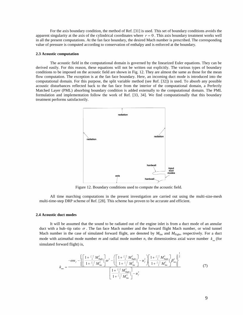
conditions to be imposed on the acoustic field are shown in Fig. 12. They are almost the same as those for the mean

flow computation. The exception is at the fan face boundary. Here, an incoming duct mode is introduced into the

computational domain. For this purpose, the split variable method (see Ref. [32]) is used. To absorb any possible

acoustic disturbances reflected back to the fan face from the interior of the computational domain, a Perfectly

Matched Layer (PML) absorbing boundary condition is added externally to the computational domain. The PML

formulation and implementation follow the work of Ref. [33, 34]. We find computationally that this boundary

treatment performs satisfactorily.

Figure 12. Boundary conditions used to compute the acoustic field.

All time marching computations in the present investigation are carried out using the multi-size-mesh

multi-time-step DRP scheme of Ref. [28]. This scheme has proven to be accurate and efficient.

2.4 Acoustic duct modes

It will be assumed that the sound to be radiated out of the engine inlet is from a duct mode of an annular

duct with a hub–tip ratio . The fan face Mach number and the forward flight Mach number, or wind tunnel

Mach number in the case of simulated forward flight, are denoted by Mfan and Mflight, respectively. For a duct

mode with azimuthal mode number m and radial mode number n, the dimensionless axial wave number kmn

(for

simulated forward flight) is,

kmn

uf

1 1

2M

flight

2

1 1

2M

fan

2

2

1 1

2M

flight

2

1 1

2M

fan

2

u f

2

1 1

2M

flight

2

1 1

2M

fan

2

mn

2

1

2

1 1

2M

flight

2

1 1

2M

fan

2

u f

2

(7)

10

where is the angular frequency, ufis the fan face velocity given by,

u f M f

1 1

2M flight

2

1 1

2M fan

2

12

and mn

is the root of the dispersion relation,

Jm

1

2mn Y

2mn Y

m

1

2mn J

m

2mn 0 (8)

Jm and Y

m are the Bessel and Neumann functions of order m. The duct mode eigenfunction is,

pmn

umn

vmn

wmn

mn

Amn

1kmn

fan kmnu f

imn

fan kmnu f

m

fan kmnu f r

1 12 1 M fan

2

1 12 1 M flight

2

Jmmnr

Jm

2mn

Ym

2mn Ymmnr

ei kmn xm t

(9)

Note: In this work, the radial mode number n is set equal to the total number of maxima and minima of the

eigenfunction. According to this numbering system, n 0 is possible only for the plane wave mode (i.e.

m n 0 ). For azimuthal modes with m 0 , the lowest order radial mode is n 1 .

Cantrell and Hart35

derived an expression for the energy flux in the upstream direction. On following their

formula, with fan face variables f, uf, af, the energy flux, Fmn

, for the (m,n) duct mode is found to be,

Fmn Q

mnAmn

21 u

f

1 1

2M

fan

2

1 1

2M

flight

2

kmn

f k

mnuf uf

f

kmn

2

kmnuf

2

1

af

2

(10)

where

Qmn

1

81 2 , m n 0, mn 0

Jm mnr Jm mn

2

Ym mn2 Ym mnr

2

r dr, mn 0 /2

1/2

If PWL is the sound power level of the (m,n)

th duct mode in dB and W0 1012 watts is the reference sound

power level for the dB unit, the duct mode amplitude can easily be found to be,

Amn W010PWL /10

0a0

3D2Qmn 1 u f2

1 1

2M f

2

1 1

2M 0

2

k

f ku f u f

f

k2

ku f 2

1

a f2

1

2

(11)

11

Figure 13. Variation of duct mode axial wavelength with frequency. M

fan 0.4, M

flight 0, m 22.

Of interest later on is the dependence of the axial wavelengths of duct modes on frequency and azimuthal

mode number. The axial wavelength of the (m,n)th

mode, mn

, is related to the axial wave number kmn

of Eq. (7) by

mn 2 / kmn . Thus by examining the numerator of Eq. (7), it is easy to see that for fixed values of Mfan

, Mflight

, m

and n, an increase in frequency leads to an increase in kmn

and hence a decrease in wavelength. Fig. 13 shows typical

examples of the reduction in axial wavelength with increase in frequency.

Figure 14. Variation of duct mode axial wavelength with azimuthal mode number.

Mfan 0.4, M

flight 0 , f 6400 Hz

The eigenvalue mn

of Eq. (7) is the root of Eq. (8). It is well known that for a fixed radial mode number n,

the value of mn

from Eq. (8) increases with m. Because of this, it follows from Eq. (7) that for fixed Mfan

, Mflight

,

12

n and frequency f or , a decrease in azimuthal mode number m would lead to an increase in kmn

and, therefore, a

reduction in axial wavelength. Fig. 14 shows typical examples of the variation of mn

with m.

2.5 Extension to the far field

A computational domain inevitably has a finite size. To determine far field directivity, it is, therefore,

necessary to extend the numerical solution to the far field. Currently, the Kirchhoff method and the Ffowcs Williams

and Hawkings method36

(see also Pilon and Lyrintzis37

and Lyrintzis38

) are the two most popular methods for

extending near field results to the far field. To use these methods, one encloses the near field by a matching surface.

The extension is to continue the information prescribed on the matching surface to the far field. In both the

Kirchhoff method and the Ffowcs Williams and Hawkings method, at least three sets of data are required on the

matching surface. The data needed are the pressure, the normal gradient of the pressure on the surface and the time

derivative of pressure. Recently, Reba, Simonich and Schlinker39

, Reba, Narayanan, Colonius and Suzuki40

and

Tam, Pastouchenko and Viswanathan41

have shown that the near-to-far acoustic field extension, or the continuation

problem, can also be accomplished by the use of a surface Green‘s function. For the jet engine inlet duct mode

radiation problem, it turns out the surface Green‘s function method is the simplest to use and to implement. Instead

of requiring three sets of data as the Kirchhoff method and the Ffowcs Williams and Hawkings method, the surface

Green‘s function method requires only one set of data, namely, the value of pressure on the matching surface. For

this reason, the surface Green‘s function method is adopted in this work. The mathematical details of the surface

Green‘s function method for the jet engine inlet noise radiation problem are given in Appendix A.

3. Code Validation

To validate the computer code developed in this investigation, the JT15D static engine test data is used.

Details of this experiment can be found in the papers by Heidelberg, Rice and Homyak36

, Baumeister, and

Horowitz14

, and Preisser, Silcox, Eversman, and Parrett2. This set of data has been used for code validation by

Ozyoruk, Alpman, Ahuja, and Long24

. Fig. 15 shows the geometry of the JT15D engine inlet. In the experiment, the

inlet was first tested with a hard wall surface. Then a liner segment was inserted in the casing, as shown in Fig. 15,

and the liner configuration was tested for two separate values of impedance. Hence, three sets of experimental data

are available for validation.

Figure 15. Geometry of JT15D engine inlet, including the location of a liner segment.

The fan of the JT15D engine has 28 blades operating at a blade passage frequency of 3150 Hz. The fan face

Mach number is 0.147. There are 41 small rods mounted on the casing wall ahead of the fan. The wake shed by

the rods is cut by the fan blades, creating strong interaction tones. By design, the inlet geometry and the blade

13

passage frequency support only one propagating mode with m = 13 and n = 1. The fact that there is only one

propagating mode greatly simplifies the effort to compare numerical results with experimentally measured

directivities.

Figure 16. Comparison between computed and measured directivity (hard wall).

——— computed, measured.

Fig. 16 shows a comparison between the experimentally measured and computed directivities for the hard

wall inlet. As can be seen, there is a reasonably good overall agreement. The degree of agreement is comparable

to that obtained by Ozyoruk, Alpman, Ahuja and Long24

. Figs. 17 and 18 are comparisons of measured and

computed relative directivities for the cases with a liner. In Fig. 17 the impedance of the liner is Z = 0.638+i0.5.

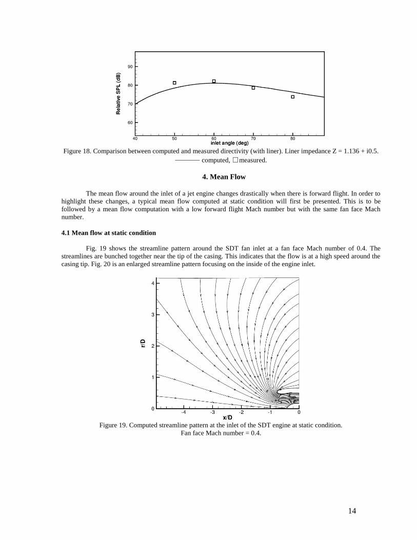
Fig. 18 shows the comparison for a liner with impedance Z = 1.136+i0.5. There are good to reasonably good

overall agreements in these cases. Again, the degree of agreement is similar to that obtained by Ozyoruk et al24

.

Figure 17. Comparison between computed and measured directivity (with liner). Liner impedance Z = 0.638 + i0.5.

——— computed, ☐ measured.

14

Figure 18. Comparison between computed and measured directivity (with liner). Liner impedance Z = 1.136 + i0.5.

——— computed, ☐ measured.

4. Mean Flow

The mean flow around the inlet of a jet engine changes drastically when there is forward flight. In order to

highlight these changes, a typical mean flow computed at static condition will first be presented. This is to be

followed by a mean flow computation with a low forward flight Mach number but with the same fan face Mach

number.

4.1 Mean flow at static condition

Fig. 19 shows the streamline pattern around the SDT fan inlet at a fan face Mach number of 0.4. The

streamlines are bunched together near the tip of the casing. This indicates that the flow is at a high speed around the

casing tip. Fig. 20 is an enlarged streamline pattern focusing on the inside of the engine inlet.

Figure 19. Computed streamline pattern at the inlet of the SDT engine at static condition.

Fan face Mach number = 0.4.

15

Figure 20. Enlarged streamline pattern inside the SDT engine inlet.

Fig. 21 plots the tangential velocity, Vtan

, along the casing wall. Fig. 21a shows the locations of selected

points A, B, C, D, E, and F along the casing wall. Fig. 21b provides a plot of the tangential velocity on the casing

versus the radial distance from the axis of the inlet. At point A, the flow velocity is practically zero, which is the

ambient condition. From A to D the flow velocity accelerates quickly to a Mach number of 0.74. This is a transonic

Mach number. It is almost twice the fan face Mach number. Along DEF the flow velocity decelerates. It reduces

further to Mach 0.4 at the fan face.

Fig. 21a. Location of points A,B,C,D,E, and F

on casing. Fig. 21b. Tangential velocity at A,B,C,D,E, and F.

Fig. 22 shows that the mean flow reaches its highest velocity at the lip of the casing. The flow is slower at

the center of the inlet. As a result, a significant velocity gradient develops as indicated in this figure. The velocity

gradient points towards the lip of the casing, toward the point with the highest velocity. The arrow in this figure

points in the direction of negative gradient.

16

Figure 22. Strong velocity gradient develops near the lip of the casing.

Arrow points in the direction of negative gradient.

4.2 Mean flow in forward flight

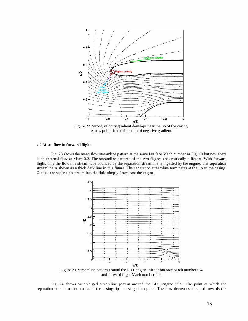
Fig. 23 shows the mean flow streamline pattern at the same fan face Mach number as Fig. 19 but now there

is an external flow at Mach 0.2. The streamline patterns of the two figures are drastically different. With forward

flight, only the flow in a stream tube bounded by the separation streamline is ingested by the engine. The separation

streamline is shown as a thick dark line in this figure. The separation streamline terminates at the lip of the casing.

Outside the separation streamline, the fluid simply flows past the engine.

Figure 23. Streamline pattern around the SDT engine inlet at fan face Mach number 0.4

and forward flight Mach number 0.2.

Fig. 24 shows an enlarged streamline pattern around the SDT engine inlet. The point at which the

separation streamline terminates at the casing lip is a stagnation point. The flow decreases in speed towards the

17

stagnation point. On passing this point on the casing wall, the flow starts to accelerate and ultimately reaches Mach

0.4 at the fan face. Now, around the lip of the casing the flow velocity is the lowest at the stagnation point. This

creates a velocity gradient pointing away from the casing wall. It is to be noted that the direction of the velocity

gradient is opposite in the case with no forward flight, as shown in Fig. 22. This contrast in the direction of the

velocity gradient for static and flight conditions turns out to be rather significant, as will be seen in the following

section.

Figure 24. Mean velocity gradient developed near the lip of the casing at forward flight Mach number 0.2.

5. Diffraction and Refraction

In this section, duct mode radiation patterns and directivities computed with and without forward flight are

presented. The directivities with forward flight are quite different from those without. The reason for this difference

will be explained below. Two effects are most important in affecting the direction of radiation. They are: diffraction

and refraction. Essentially, the combination of these two effects determines the radiation pattern of a duct mode.

5.1 Diffraction

In the context of duct mode radiation, we will define diffraction as the natural tendency of the pressure field

of a duct mode to follow a curved solid surface as it propagates. This effect causes the wave field‘s direction of

propagation to make a large turn at the lip of an engine casing. To illustrate this process, consider a duct mode of m

= 22, n = 1 at a frequency of 6.4 kHz radiating out of the SDT engine inlet. We will first study the case without

mean flow. That is, the fan face Mach number is zero. This allows us to investigate the propagation of duct modes

along the casing wall without any modification by the mean flow. Fig. 25 shows the radiation pattern. The lines are

pressure contours. In this figure, red is high pressure and blue is low pressure. The duct mode does not propagate

straight out of the inlet in the forward direction. At the casing lip, the sound field turns at an angle of about 45

degrees before radiating away.

18

Figure 25. Near field pressure contour pattern showing the dominant direction of radiation.

No mean flow. Duct mode has m = 22, n = 1.

Figure 26. A schematic sketch illustrating the complete separation of a duct mode from the casing wall

when radiating out of an engine inlet. Required pressure balance prevents this type of complete separation.

Now, a duct mode is made up of alternating high and low pressure regions. The highest and the lowest

pressure points are right next to the wall, as shown in Figs. 25 and 26. When the sound field propagates along a solid

surface, the surface can sustain the high and low pressure variations. Suppose the duct mode propagates in a strictly

forward direction, separating from the casing surface as shown in Fig. 26. Immediately, there would be a pressure

imbalance along the line of separation because the ambient pressure is constant. Thus, the pressure field of the duct

mode must adjust its pressure distribution by shifting the highest and lowest pressure points away from the wall

while it remains attached to the wall, as shown in Fig. 27a. Fig. 27b shows a diffraction pattern (pressure contours)

at 6400 Hz for a duct mode with m = 22 and n = 1. The attachment of the sound field to the casing wall is clearly

shown.

19

Figure 27a. To maintain pressure balance, a radiating duct mode must adjust its pressure distribution and remain

attached to the casing wall. The adjustment causes the direction of propagation to rotate in the clockwise direction.

Figure 27b. Instantaneous distribution of pressure contours associated with the radiation of a duct mode with m = 22

and n = 1 at 6400 Hz from the SDT engine inlet.

Diffraction causes the pressure field to rotate in the clockwise direction. As the duct mode turns, the highest

and lowest pressure regions gradually move away from the wall. When the highest and lowest pressure regions have

detached sufficiently from the wall, the sound field can then radiate away. These processes are observable in a high-

speed animation. Thus, the effect of diffraction is what leads the duct mode in Fig. 25 to radiate predominantly

around the 45° direction.

The effect of diffraction naturally depends on the axial wavelength of the duct mode. For duct modes with

short wavelengths, the diffraction effect is small. This should become clear if one considers the limit of very small

wavelengths. In this limit, the sound waves are rays, like that of light. If light waves were to radiate out of an engine

inlet, they would mostly radiate in the forward direction. In other words, the diffraction effect is absent or minimal.

What this reasoning suggests is that the diffraction effect is stronger for long waves and less significant for short

waves. Fig. 28 shows the diffraction pattern of duct modes with m = 22 and n = 1 at a range of frequencies from 5.2

kHz to 7.6 kHz. It is obvious that at low frequencies the axial wavelength is longer (see Fig. 13). For these long

waves, the turning angle of the direction of radiation (clockwise) measured from the inlet direction is larger. This is

consistent with the above deduction. Fig. 29 is a symbolic representation of the dependence of the turning angle on

20

wavelength. In this figure, 1

2

3 implies decreasing wavelength. The radius of the arc of rotation and the

thickness of the arc in the figure represent the relative size of the angle of rotation. The point is: the shorter the

wavelength, the smaller the clockwise turning angle from diffraction.

Figure 28. Pressure contour patterns showing the radiation of duct modes from the SDT engine inlet (without mean

flow) at a number of frequencies. All duct modes have respective azimuthal and radial mode numbers of m = 22 and

n = 1.

Figure 29. Symbolic representation of the dependence of diffraction effect on duct mode wavelength.

5.2 Refraction

A jet engine draws in a large quantity of air at its inlet. As discussed in the previous section, this creates a

nonuniform mean flow with a significant velocity gradient around the casing lip. At a fan face Mach number of 0.4,

in static condition, the mean flow causes the radiation pattern to change from Fig. 25 to Fig. 1. Fig. 30 is a

superposition of the two radiation patterns. It is clear that the presence of a mean flow causes the dominant direction

of radiation to rotate in the clockwise direction almost an additional 45° past the angle caused by diffraction only.

This substantial change in the radiation direction is due to the effect of refraction. At static condition, the velocity

gradient near the casing lip is shown in Fig. 22. Now consider a wave front AA′ as shown in Fig. 31. The wave is

propagating against the flow. The flow velocity is highest along the casing wall AB and much slower along

streamline A′B′. Thus the propagation speed, being equal to the speed of sound minus the flow velocity, is faster

21

along A′B′ than along AB. As a result, the wave front will rotate in the clockwise direction. This turns the direction

of radiation farther to the right, resulting in an almost 80° direction of propagation (inlet angle).

Figure 30. Pressure contours showing the change in the dominant direction of radiation when the fan face Mach

number increases from zero (no mean flow, gray) to 0.4 at static condition (green). m = 22, n = 1, f = 6400Hz.

Figure 31. Propagation of wave fronts AA′ and BB′ along the casing wall at static condition. The wave front rotates

in the clockwise direction upon encountering gradients in the mean flow velocity. This is the refraction effect.

For a jet engine in forward flight, the effect of refraction is quite different. Fig. 32 shows the radiation

pattern for three mean flow conditions: zero mean flow, static condition, and flight condition. When there is no

mean flow, the diffraction effect rotates the dominant direction of radiation to about 45°. In the presence of a mean

flow at static condition, refraction further rotates the dominant direction of radiation clockwise to nearly 80°.

However, with a forward flight Mach number of 0.2, the refraction effect rotates the dominant direction of radiation

by about 10° counterclockwise off the angle caused by diffraction only. This counterclockwise rotation is not

difficult to understand. With forward flight, the mean flow pattern and velocity gradients are shown in Fig. 24. The

velocity gradient is almost in opposite direction to that in the static case (see Fig. 22). However, the gradient is

milder and occurs over a shorter distance along the casing wall. Again consider the wave fronts AA′ and BB′ as

22

shown in Fig. 33. This time the flow velocity along the casing lip, i.e., AB, is slower than that along A′B′. As a

result, the wave front propagates faster along AB than A′B′. This causes a counterclockwise rotation in the direction

of wave propagation. This explains the counterclockwise rotation of the dominant direction of radiation for a jet

engine in forward flight as observed in Fig. 32. It is to be noted for forward flight condition that the combined effect

of diffraction and refraction results in an overall clockwise rotation in the direction of wave propagation. This

indicates that the diffraction effect is the more dominant process.

Figure 32. Pressure contours showing the dominant direction of radiation when there is no mean flow (green), when

there is a mean flow at static condition (blue; fan face Mach number = 0.4) and when there is a forward flight at

Mach 0.2 (red). m = 22, n = 1 and f = 6400 Hz.

Figure 33. Propagation of wave fronts AA′ and BB′ when there is a Mach 0.2 forward flight.

Here, refraction causes a counterclockwise rotation in propagation.

Just as for diffraction, the effect of refraction is also dependent on the duct mode axial wavelength. Fig. 34

illustrates the propagation of a long wave and a short wave through a region with a localized velocity gradient.

Relative to the long wave, the region is small and hence its effect on the wave is minimal. Relative to the short

23

wave, the nonuniform flow region is quite large. Thus, the velocity gradient effect is significant. Another way of

reaching the same conclusion is by considering the limit of wavelength >> length of velocity gradient region. In

this limit, the wave effectively does not see the velocity gradient and hence should experience little effect. On the

other hand, for waves with wavelengths much shorter than the size of the nonuniform velocity region, one expects

the wave to experience the full strength of refraction when traversing the region. Thus the direction of propagation

of short waves would be severely turned by refraction, whereas long waves would not be much affected. This

observation is summarized symbolically in Fig. 35. In this figure, the case of an engine in static condition is

considered separately from the same engine in flight. This is because in static condition, refraction causes the wave

propagation direction to rotate in the clockwise direction, while for an engine in forward flight, the refraction effect

causes a counterclockwise rotation in the direction of propagation. In both cases, the angle of rotation increases with

a decrease in axial wavelength.

Figure 34. Schematic diagram of the propagation of a long and a short wave through a localized region of velocity

gradient.

Figure 35. Symbolic representation of dependence of refraction effect on wavelength. Size of arc indicates the

magnitude of rotation due to velocity gradient.

6. Parametric Study of Acoustic Radiation

We have seen that forward flight has a significant impact on duct mode radiation patterns and directivity. A

duct mode is characterized by its azimuthal mode number, radial mode number, and frequency. In this section, the

results of a parametric study of the effects of forward flight Mach number, frequency and mode numbers are

presented.

24

6.1 Forward flight effect The mean flow around an engine inlet changes with forward flight Mach number. Fig. 36 shows the

separation streamlines and stagnation point locations for forward flight Mach numbers 0.15, 0.2 and 0.25. This

figure shows that as flight Mach number increases, the location of the stagnation point on the casing lip becomes

somewhat insensitive to further increase after Mflight exceeds 0.15. Fig. 37 is similar to Fig. 21b. It shows the change

in flow velocity on the surface of the casing as flight Mach number increases. At zero forward flight Mach number,

the velocity on the surface of the casing can speed up to transonic. But for higher flight Mach numbers, the

maximum surface velocity is about the same as that at the fan face. This means the refraction effect diminishes at

high flight Mach numbers.

Figure 36. Change in the location of stagnation point as forward flight Mach number increases.

Figure 37. Changes in tangential velocity on engine inlet casing wall as forward flight Mach number increases.

25

The effect of forward flight Mach number on directivity is illustrated in Fig. 38. It is clear that there is a

saturation effect, namely, beyond flight Mach number 0.15 there is no substantial change in the directivity. A more

simplistic way to see this is to look at the direction of maximum radiation. This is shown in Fig. 39. This saturation

effect on the impact of increasing flight Mach number occurs because the mean flow undergoes only minor changes

in response to such increase beyond 0.15, as was shown in Figs. 36 and 37. Any further refraction effect is minimal,

leading to little change in directivity.

Figure 38. Directivity of the radiation of duct mode m = 22, n = 1, f = 5600 Hz (fan face Mach number 0.4) at

varying forward flight Mach numbers.

Figure 39. Direction of maximum sound radiation at varying forward flight Mach numbers.

Duct mode with m = 22, n = 1, f = 5600 Hz, and fan face Mach number 0.4.

26

6.2 Frequency variation

The axial wavelength of a duct mode changes with frequency. Fig. 13 shows the dependence of the duct

mode axial wavelength on frequency for the case M fan 0.4 at static condition. As discussed before, both

diffraction and refraction effects are axial-wavelength dependent. To investigate the dependence of the directivity of

radiation on frequency, we will consider the case M fan 0.4 , m = 22 and n = 1. Fig. 40 shows the pressure contour

patterns at static condition, i.e., M flight 0 , when the duct mode frequency varies from 4.5 to 6.4 kHz. It is clear

from this figure that the pattern changes only slightly with frequency. Now, let us consider the case at forward flight

Mach number 0.2. The pressure contour patterns are displayed in Fig. 41. At M flight 0.2 , the dominant direction of

radiation is a strong function of frequency. Higher-frequency duct modes radiate at lower inlet angles. Thus, there is

a significant difference in the radiation pattern with and without forward flight. This phenomenon may also be

observed by considering directivity. The directivities are shown in Fig. 42 for M flight 0 and Fig. 43 for M flight 0.2 .

Again, there is little frequency dependence at the static condition, but a significant dependence exists when there is

forward flight.

Figure 40. Pressure contour pattern of duct mode radiation. M

fan 0.4, M

flight 0, m 22, n 1,

with frequencies varying over f = 4.5, 4.8, 5.4, 5.6 and 6.4 kHz.

Figure 41. Pressure contour pattern of duct mode radiation. M

fan 0.4, M

flight 0.2, m 22, n 1,

with frequencies varying over f = 4.5, 4.8, 5.4, 5.6 and 6.4 kHz.

27

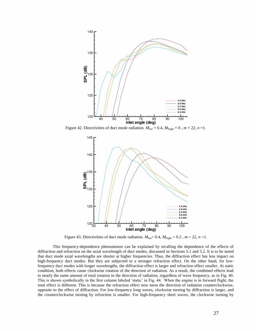
Figure 42. Directivities of duct mode radiation. Mfan = 0.4, Mflight = 0 , m = 22, n =1.

Figure 43. Directivities of duct mode radiation. Mfan= 0.4, Mflight = 0.2 , m = 22, n =1.

This frequency-dependence phenomenon can be explained by recalling the dependence of the effects of

diffraction and refraction on the axial wavelength of duct modes, discussed in Sections 5.1 and 5.2. It is to be noted

that duct mode axial wavelengths are shorter at higher frequencies. Thus, the diffraction effect has less impact on

high-frequency duct modes. But they are subjected to a stronger refraction effect. On the other hand, for low-

frequency duct modes with longer wavelengths, the diffraction effect is larger and refraction effect smaller. At static

condition, both effects cause clockwise rotation of the direction of radiation. As a result, the combined effects lead

to nearly the same amount of total rotation in the direction of radiation, regardless of wave frequency, as in Fig. 40.

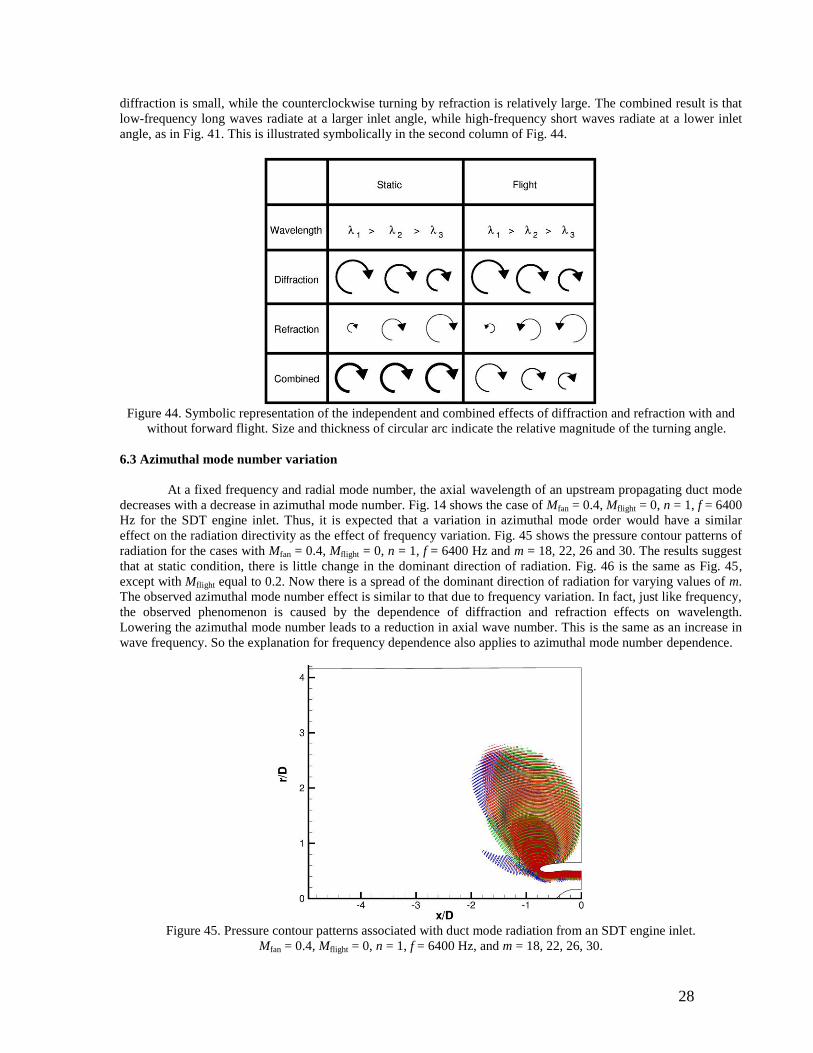
This is shown symbolically in the first column labeled ‗static‘ in Fig. 44. When the engine is in forward flight, the

total effect is different. This is because the refraction effect now turns the direction of radiation counterclockwise,

opposite to the effect of diffraction. For low-frequency long waves, clockwise turning by diffraction is larger, and

the counterclockwise turning by refraction is smaller. For high-frequency short waves, the clockwise turning by

28

diffraction is small, while the counterclockwise turning by refraction is relatively large. The combined result is that

low-frequency long waves radiate at a larger inlet angle, while high-frequency short waves radiate at a lower inlet

angle, as in Fig. 41. This is illustrated symbolically in the second column of Fig. 44.

Figure 44. Symbolic representation of the independent and combined effects of diffraction and refraction with and

without forward flight. Size and thickness of circular arc indicate the relative magnitude of the turning angle.

6.3 Azimuthal mode number variation

At a fixed frequency and radial mode number, the axial wavelength of an upstream propagating duct mode

decreases with a decrease in azimuthal mode number. Fig. 14 shows the case of Mfan = 0.4, Mflight = 0, n = 1, f = 6400

Hz for the SDT engine inlet. Thus, it is expected that a variation in azimuthal mode order would have a similar

effect on the radiation directivity as the effect of frequency variation. Fig. 45 shows the pressure contour patterns of

radiation for the cases with Mfan = 0.4, Mflight = 0, n = 1, f = 6400 Hz and m = 18, 22, 26 and 30. The results suggest

that at static condition, there is little change in the dominant direction of radiation. Fig. 46 is the same as Fig. 45,

except with Mflight equal to 0.2. Now there is a spread of the dominant direction of radiation for varying values of m.

The observed azimuthal mode number effect is similar to that due to frequency variation. In fact, just like frequency,

the observed phenomenon is caused by the dependence of diffraction and refraction effects on wavelength.

Lowering the azimuthal mode number leads to a reduction in axial wave number. This is the same as an increase in

wave frequency. So the explanation for frequency dependence also applies to azimuthal mode number dependence.

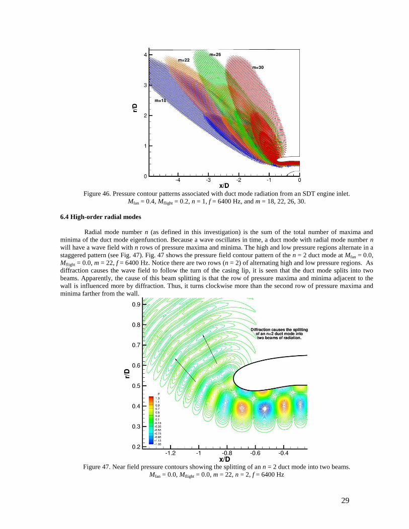
Figure 45. Pressure contour patterns associated with duct mode radiation from an SDT engine inlet.

Mfan = 0.4, Mflight = 0, n = 1, f = 6400 Hz, and m = 18, 22, 26, 30.

29

Figure 46. Pressure contour patterns associated with duct mode radiation from an SDT engine inlet.

Mfan = 0.4, Mflight = 0.2, n = 1, f = 6400 Hz, and m = 18, 22, 26, 30.

6.4 High-order radial modes

Radial mode number n (as defined in this investigation) is the sum of the total number of maxima and

minima of the duct mode eigenfunction. Because a wave oscillates in time, a duct mode with radial mode number n

will have a wave field with n rows of pressure maxima and minima. The high and low pressure regions alternate in a

staggered pattern (see Fig. 47). Fig. 47 shows the pressure field contour pattern of the n = 2 duct mode at Mfan = 0.0,

Mflight = 0.0, m = 22, f = 6400 Hz. Notice there are two rows (n = 2) of alternating high and low pressure regions. As

diffraction causes the wave field to follow the turn of the casing lip, it is seen that the duct mode splits into two

beams. Apparently, the cause of this beam splitting is that the row of pressure maxima and minima adjacent to the

wall is influenced more by diffraction. Thus, it turns clockwise more than the second row of pressure maxima and

minima farther from the wall.

Figure 47. Near field pressure contours showing the splitting of an n = 2 duct mode into two beams.

Mfan = 0.0, Mflight = 0.0, m = 22, n = 2, f = 6400 Hz

30

This beam-splitting phenomenon for the second radial mode is affected by forward flight Mach number.

Figs. 48a–48c show the change in the pressure contour pattern for the case Mfan = 0.4, m = 22, f = 5600 Hz, as flight

Mach number increases. Fig. 48a corresponds to Mflight = 0.0; Fig. 48b is for Mflight = 0.15; and Fig. 48c for Mflight =

0.25. By comparing these figures, it should be obvious that forward flight has a significant influence on the radiation

pattern and directivity. Fig. 49 is a directivity plot for Mflight = 0.05, 0.1, 0.15, 0.2 and 0.25. There are basically two

beams of radiation. As flight Mach number increases, there is a gradual changeover in the dominancy of the two

beams. At low flight Mach numbers, the beam radiated to the lower inlet angle is the dominant beam. As Mflight

increases, a gradual shift in dominancy takes place. By Mflight = 0.15, the shift is nearly complete. Beyond 0.15, the

beam that radiates to the higher inlet angle is the dominant beam.

Figure 48a. Radiation pattern from an n = 2 duct mode with m = 22, Mfan = 0.4, Mflight = 0.0, f = 5600 Hz.

Figure 48b. Radiation pattern from an n = 2 duct mode with m = 22, Mfan = 0.4, Mflight = 0.15, f = 5600 Hz.

31

Figure 48c. Radiation pattern from an n = 2 duct mode with m = 22, Mfan = 0.4, Mflight = 0.25, f = 5600 Hz.

Figure 49. Directivity of sound in the far field radiated by an n = 2 duct mode with m = 22, Mfan = 0.4, f = 5600 Hz.

Fig. 50 shows the results of taking an even higher radial mode number: Mfan = 0.4, Mflight = 0.2, m = 22, n =

4, f = 6800 Hz. Upon radiating out of the engine inlet, the four rows of high and low pressure regions merge into two

beams. It is to be noted that the radial mode number n is meaningful inside the duct and in the part of the inlet close

to the fan face. Once the sound waves exit the inlet, the radial mode number is no longer meaningful. Therefore, at

the engine inlet, there is a region in which a high-order radial mode would undergo a transformation whereby the

multi-layer pressure field structure combines into a single sinusoidal spatial structure typical of far field propagating

acoustic waves. In addition, inside an engine inlet, the sound field of a duct mode has an axial wavelength

determined by frequency, azimuthal mode number, mean flow Mach number and the diameter of the duct. But once

the sound field exits the inlet, the wavelength of the freely propagating acoustic wave depends solely on its

frequency. Therefore, there is also an adjustment of wavelength in the transition region. This wavelength transition

32

also applies to duct modes with n = 1 radial mode number. Fig. 51 shows the transition for an n = 4 duct mode in the

engine inlet.

Figure 50. Radiation pattern for an n = 4 duct mode with m = 22, Mfan = 0.4, Mflight = 0.2, f = 6800 Hz. The four rows

of high and low pressure fluctuations near the fan face eventually radiate out of the inlet as two beams.

Figure 51. Pressure contours showing the transition region at the inlet of an engine for an n = 4 duct mode.

m = 22, Mfan = 0.4, Mflight = 0.0, f = 6800 Hz.

7. Summary and Conclusion

Numerical simulation of duct mode radiation from a jet engine inlet is carried out. An advanced CAA time

marching algorithm and high-quality numerical boundary conditions are used. The computational code is validated

by comparing predicted directivities for the JT15D engine with experimental measurements.

33

Computed results are used to highlight the important physical processes that affect the sound radiation

pattern and directivity. It is demonstrated that the phenomena of diffraction and refraction play a key role in

determining the ultimate direction of radiation. Diffraction is the natural tendency for a duct mode to follow a

curved solid surface as it propagates. Refraction is the bending of the direction of sound propagation by a mean flow

velocity gradient. It is shown that the mean flow velocity distribution around an engine inlet in forward flight differs

markedly from that in static operating condition. For this reason, there is a substantial change in the duct mode

radiation pattern and directivity when switching from static condition to forward flight condition. However, as flight

Mach number increases beyond 0.15, there are only minor changes in the mean flow. In other words, the forward

flight effect exhibits a saturation phenomenon. That is, further increase in forward flight Mach number above 0.15

would bring about little change in the duct mode radiation directivity.

In this investigation, a parametric study of the effect of frequency and azimuthal mode number on inlet

acoustic radiation has been carried out. Both frequency and azimuthal mode number affect the axial wavelength of a

duct mode. It is found that a change in axial wavelength affects the level of influence of diffraction and refraction.

Refraction exerts a larger impact on short waves than on long waves. Thus duct modes with higher frequencies or

lower azimuthal mode numbers are more affected by refraction. On the other hand, diffraction has a larger effect on

duct modes with long axial wavelengths. Because of these differences in axial-wavelength dependence, when the

frequency or azimuthal mode number changes, the combined effect of diffraction and refraction causes most duct

modes at static condition to radiate at a relatively consistent angle in the sideline direction (approximately 80° inlet

angle) and duct modes at forward flight condition to radiate at a range of angles in the forward direction.

A duct mode with a radial mode number n has n rows of alternating high and low pressure regions. At the

casing lip region, because different rows are at different distances from the wall, they are subjected to different

degrees of diffraction and refraction. This results in the splitting of the radiation pattern into multiple beams. The

results of a brief study of this effect on duct modes with high-order radial mode numbers is reported.

It seems worthwhile to emphasize, based on the numerical simulation results of the present investigation,

that the duct mode radiation pattern from a jet engine inlet in forward flight is quite different from that in static

condition. This suggests, for community noise prediction purposes, there is no simple scaling formula that can

convert the radiation pattern from the static condition to the flight condition. It is also recognized that there is no

simple way to create a stagnation point, a distinct characteristic of forward flight, on the casing lip of an engine in a

static test condition. Therefore, static engine test data might not be of use for engines in flight. Hence, their

usefulness is very limited.

Before the advent of fast computers, sound radiation from engine inlets was investigated using a somewhat

idealized model. The work of Homicz and Lordi11

, Candel43

, Wright44

and others adopted a zero-thickness

cylindrical inlet model. One main advantage of such a model is that the duct mode radiation problem can be solved

exactly by the Wiener-Hopf technique. These early works were later summarized and extended by Rice, Heidmann

and Sofrin45

to form a prediction formula for the direction of peak noise radiation. The most general formula of Rice

et al. was designed to be applicable to inlet radiation at static as well as at flight condition. In their paper, they

pointed out that in deriving their formula, only the mean flow convection effect was included. The refraction effect

was entirely neglected. In a real engine, the engine casing has a finite thickness. As was discussed earlier in Section

5, this thickness is very important to the processes of diffraction and refraction. Setting this thickness to zero may

lead to severe prediction error.

34

Figure 52. Peak direction of radiation for a duct mode with m = 22, n = 1 as a function of dimensionless frequency

with no mean flow. ——— Rice et al. theory45

(zero-thickness cylindrical inlet), numerical simulation (SDT

engine inlet).

As an illustration of the influence of inlet casing thickness on the effect of diffraction, a comparison

between the computed peak direction of radiation from an SDT engine inlet using numerical simulation and that

from a zero-thickness cylindrical inlet of the same diameter using the Rice et al. theory45

(in the absence mean flow)

is made. Fig. 52 shows a comparison of the computed peak directions of radiation for a duct mode with m = 22 and

n = 1 as a function of frequency. The relevant parameter, important to the diffraction process, is the ratio of casing

thickness to the axial wavelength of the duct mode. For the SDT inlet, this ratio is finite; for the zero-thickness

cylindrical inlet, this ratio is zero. At low frequencies, the duct mode axial wavelength is long, so the thickness-to-

wavelength ratio is small. In this case, one would expect the two predictions to be fairly close. This is confirmed in

Fig. 52. As frequency increases, this ratio becomes larger and larger for the SDT inlet. It follows that the difference

between the two computed peak directions of radiation becomes larger and larger. This is evident in Fig. 52.

35

Figure 53. Peak direction of radiation for a duct mode with m = 22, n = 1 as a function of dimensionless frequency.

Static engine test with Mfan = 0.4. ——— Rice et al theory45

(zero-thickness cylindrical inlet), numerical

simulation (SDT engine inlet).

As an illustration of the importance of including mean flow refraction in the prediction of duct mode

radiation, a comparison is made between the result of using the classical theory of Rice et al.45

and that obtained by

numerical simulation for the SDT engine inlet at static test condition. Fig. 53 shows the peak directions of radiation

for a duct mode with m = 22 and n = 1 at different dimensionless frequencies. It is clear that there are huge

differences between the two predictions. Based on this result and the comparisons made in Fig. 52, we conclude

that for an accurate prediction of jet engine inlet acoustic radiation, it is imperative that the physical processes of

diffraction and refraction be properly incorporated in the formulation of a theory or a computational model.

Appendix A. Extension of near acoustic field to far field by the surface Green’s function method

For the jet engine inlet noise radiation problem, a good matching surface for the extension of near field to

far field is an infinitely long cylindrical surface enclosing the engine. For convenience, we set the matching

cylindrical surface to be 3 mesh points inside the computational domain of Fig. 3. The generator of the cylindrical

surface is parallel to the line BD. In all the validation directivity computations, the computational domain is

extended to a distance of 10 fan diameters in the axial direction from the fan face. This extended domain is 5

diameters larger than the computational domain from the near field pressure contour study. This larger

computational domain ensures that most of the sound waves radiated from the engine inlet pass through the

matching surface.

Let the diameter of the matching cylindrical surface be DM and the forward flight Mach number be M

(i.e., M M

flight). Outside the matching cylindrical surface, the linearized Euler equation and energy equations are,

v

t M

v

x p (A1)

p

t M

p

x v 0 (A2)

Upon eliminating v from Eqs. (A1) and (A2), the governing equation for p is,

t M

x

2

p 2p 0 (A3)

The surface Green‘s function G r,, x, t;0, x

0, t

0 , where r,, x, t are the far field observer coordinates

and time and 0, x

0, t

0 are the source coordinates on the matching surface and time, satisfies the same governing

equation as p (Eq. (A3)) together with boundary conditions as follows:

t M

x

2

G 2G 0 (A4)

At r2 x

2 1

2

, G behaves as outgoing waves (A5)

At r 1

2DM

, G x x

0

0 t t

0

1

2DM

(A6)

36

Let the radiated pressure field be from a duct mode of azimuthal mode number m, radial mode number n,

and frequency . On the matching surface, the pressure field is,

p Re p x ei m t . (A7)

By means of the Green‘s function, the sound field at a far field point r,, x, t is given by,

p r,, x, t Re p x0

ei m0t

0

G r,, x, t;0, x

0, t

0

DM

2d

0dx

0dt

0

0

2

(A8)

To find G , let its Fourier transform in x and t be G , defined as,

G r,, k,;0, x

0, t

0

1

2 2G r,, x, t;

0, x

0, t

0

e i kx t

dxdt (A9)

G is periodic in . Thus, Gmay be expanded as a Fourier series in in the form,

G r,, k,;0, x

0, t

0 g

n

n

ein

(A10)

On applying Fourier transforms in x and t to Eq. (A4) and on expanding G as in Eq. (A10), it is easy to

find that gnis given by the solution of the Bessel equation,

d

2gn

dr2

1

r

dgn

drn

2

r2gn M

k 2

k2 gn 0 (A11)

From Eq. (A6), the boundary condition for gn at r D

M/ 2 is,

gn

1

43DM

e i kx

0 n

0 t

0

(A12)

In deriving Eq. (A12), the -function expansion,

0

1

2ein

0

n

(A13)

has been used. The solution of Eq. (A11) satisfying radiation boundary condition at r2 x

2 1

2

and boundary

condition (A12) is,

gn

1

43DM

Hn

1 i 1 M

2 1

2

k k

1

2 k k

1

2 r

Hn

1 i 1 M

2 1

2

k k

1

2 k k

1

2 1

2DM

e i kx

0 n

0 t

0

(A14)

where k

1 M

, k

1 M

and Hn

1 is the nth

-order Hankel function of the first kind. The branch cut of

the square root function and the inverse k-contour are as shown in Fig. A1.

37

Figure A1. Branch cut for k k

1

2 k k

1

2 in the k-plane and the inverse Fourier transform contour.

On substituting solution (A14) into Eq. (A10) and upon performing inverse transforms, the surface Green‘s

function is found to be,

G 1

43DM

Hn

1 i 1 M

2 1

2

k k

1

2 k k

1

2 r

Hn

1 i 1 M

2 1

2

k k

1

2 k k

1

2 1

2DM

ei k x x

0 t t

0 n

0

dk d

n

(A15)

For the far field solution, it is advantageous to switch to spherical polar coordinates R,, with the polar

axis coinciding with the x-axis. The relationship between the spherical polar coordinates and the cylindrical

coordinates are,

x Rcos, r Rsin (A16)

where is the polar angle. Now, for R ,G , as given by Eq. (A15), may be greatly simplified by first using the

asymptotic form of the Hankel function, then evaluating the k-integral by the method of stationary phase. The

stationary phase point is at k

1M

2

cos

1M

2sin

2

1

2

M

. This gives,

G 1

23DM

1 M

2sin

2

1

2

R

e

iR

M cos 1M

2sin

2

1

2

Hn

1 DM

sin

2 1 M

2sin

2

1

2

n

e

i

1M

2 cos

1M

2sin

2

1

2

M

x0

ei n -0 t t0 n1

2 d

(A17)

38

On inserting the surface Green‘s function (A17) into Eq. (A8), the far field pressure at R corresponding to a

duct mode of azimuthal mode number m and angular frequency can be found by evaluating the integrals

d0dt

0dx

0d . The d

0 and dt

0 integration can be carried out easily using,

ei m n

0 d0

0

2

2mn

(A18)

e i t

0 dt0

2 (A19)

Because of the delta function from Eq. (A19), the d integral can also be evaluated. This gives the

following formula, which involves a single integral, for the far field pressure,

p R,,, t Re1

1 M

2sin

2

1

2

R

e

iR

M cos 1M

2sin

2

1

2

i m t m1 2

Hm

1 DM

sin

2 1 M

2sin

2

1

2

I

R

(A20)

where

I p x

0

e

i

1M

2 cos

1M

2sin

2

1

2

M

x0

dx0

(A21)

Acknowledgements

The work done by the third author was funded by the Subsonic Fixed Wing Project of NASA‘s

Fundamental Aeronautics Program.

39

References

1Heidmann, M.F., Saule, A.V., and McArdle, J.G., ―Predicted and Observed Modal Radiation Pattern from

JT15D Engine with Inlet Rods,‖ Journal of Aircraft, Vol. 17, No. 7, 1980, pp. 493-499. 2Preisser, J.S., Silcox, R.J., Eversman,W., and Parrett, A.V., ―Flight Study of Induced Turbofan Acoustic

Radiation with Theoretical Comparisons,‖ Journal of Aircraft, Vol. 22, No. 1, 1985, pp. 57-62. 3Herkes, W.H., Olser, R.F., and Uellenberg, S., ―The Quite Technology Demonstrator Program: Flight

Validation of Airplane Noise-Reduction Concepts,‖ AIAA Paper 2006-2720, May 2006. 4Yu, J., Nesbitt, E., Kwan, H.W., Uellenberg, S., Chien, E., Premo, J., Ruiz, M., and Czech, M., ―Quite

Technology Demonstrator 2 Intake Liner Design and Validation,‖ AIAA Paper 2006-2458, May 2006. 5Callender, B., Janardan, B. Uellenberg, S., Premo, J., Kwan, H.W., Abeysinghe, A., ―The Quite

Technology Demonstrator Program: Static Test of an Acoustically Smooth Inlet,‖ AIAA Paper 2007-3671, May

2007. 6Lan, J., Premo, J. Zlavog, G., Breard, C., Callender, B., and Martinez, M., ―Phased Array Measurements

of Full-Scale Engine Inlet Noise,‖ AIAA Paper 2007-3434, May 2007. 7Premo, J., and Joppa, P., ―Fan Noise Source Diagnostic Test - Wall Measured Circumferential Array

Mode Results,‖ AIAA Paper 2002-2429, May 2002. 8Heidelberg, L., ―Fan Noise Source Diagnostic Test - Tone Modal Structure Results,‖ AIAA Paper 2002-

2428, May 2002. 9Woodward, R.P., Huges, C.E., Jeracki, R.J., and Miller, C.J., ―Fan Source Diagnostic Test – Far Field

Acoustic Results,‖ AIAA Paper 2002-2427, May 2002. 10

Lansing, D.L., ―Exact Solution for Radiation of Sound from a Semi-Infinite Circular Duct with

Application to Fan and Compressor Noise,‖ Analytic Methods in Aircraft Aerodynamics, NASA SP-228, 1970, pp.

323-334. 11

Homicz, G.F. and Lordi, J.A., ― A Note on the Radiative Directivity Patterns of Duct Acoustic Modes,‖

Journal of Sound and Vibration, Vol. 41, No. 3, 1975, pp. 283-290. 12

Kempton, A.J., and Smith, M.G., ― Ray Theory Predictions of Sound Radiation form Realistic Engine

Intakes,‖ AIAA Paper 81-1982, 1982. 13

Dougherty , R.P., ―Nacelle Acoustic Design by Ray Tracing in Three Dimensions,‖ AIAA Paper 96-1773,

May 1996. 14

Baumeister, K.J., and Horowitz, S.J., ―Finite Element-Integral Acoustic Simulation of JT15D Turbofan

Engine,‖ ASME Journal of Vibration, Acoustics, Stress, and Reliability in Design, Vol. 106, 1984, pp. 405-413. 15

Eversman, W., Parret, A.V., Preisser, J.S., and Silcox, R.J., ―Contributions to the Finite Element Solution

of the Fan Noise Radiation Problem,‖ Transactions of the American Society of Mechanical Engineers, Vol. 107,

1985, pp. 216-223. 16

Parrett, A., and Eversman, W., ―Wave Envelope and Finite Element Approximation for Turbofan Noise

Radiation in Flight,‖ AIAA Journal, Vol. 24, No. 5, 1986, pp. 753-760. 17

Roy, I.D. and Eversman, W., ―Improved Finite Element Modeling of the Turbofan Engine Inlet Radiation

Problem,‖ ASME Journal of Vibration and Acoustics, Vol. 117, No. 1. 1995, pp. 109-115. 18

Ozyoruk, Y., and Long, L.N., ― Computation of Sound Radiation from Engine Inlets,‖ AIAA Journal,

Vol. 34, No. 5, 1996, pp.894-901. 19

Ahuja, V., Ozyoruk, Y. and Long, L.N., ―Computational Simulations of Fore and Aft Radiation from

Ducted Fans,‖ AIAA Paper 2000-1943, May 2000. 20

Ozyruk, Y., Ahuja, V., and Long, L.N., ―Time Domain Simulations of Radiation from Ducted Fans with

Liners,‖ AIAA Paper 2001-2171, May 2001. 21

Zhang, X., Chen, X., Morfey, C.L., and Nelson, P.A., ―Computation of Spinning Modal Radiation from

an Unflanged Duct,‖ AIAA Paper 2002-2475, May 2002. 22

Astley, R.J., Hamilton, J.A., Baker, N., and Kitchen, E.H., ―Modelling Tone Propagation from Turbofan

Inlets – The Effect of Extended Lip Liners,‖ AIAA Paper 2002-2449, May 2002. 23

Ozyoruk, Y., ―Parallel Computation of Forward Radiated Noise of Ducted Fans Including Acoustic

Treatment,‖ AIAA Journal, Vol. 40, No. 3, 2002, pp. 450-455. 24

Ozyoruk, Y., Alpman, E., Ahuja, V. and Long, L.N., ―Frequency-Domain Prediction of Turbofan Noise

Radiation,‖ Journal of Sound and Vibration, Vol. 270, 2004, 933-950. 25

Premo, J., Breard, C., and Lan, J., ―Prediction of the Inlet Splice Effects from the QDT2 Static Test,‖

AIAA Paper 2007-3544.

40

26Achunche, I., Astley, J., Sugimoto, R., and Kempton, A., ―Prediction of Forward Fan Noise Propagation

and Radiation from Intakes,‖ AIAA Paper 2009-3239, May 2009. 27

Tam, C.K.W. and Ju, H., ―Airfoil Tones at Moderate Reynolds Number,‖ Journal of Fluid Mechanics,

Vol. 690, 2012, pp. 536-570. 28

Tam, C.K.W. and Kurbatskii, K.A., ―Multi-size-mesh Multi-time-step Dispersion Relation Preserving

Scheme for Multiple-scales Aeroacoustics Problems,‖ International Journal of Computational Fluid Dynamics, Vol.

17, 2003, pp. 119-132. 29

Tam, C.K.W. and Hu, F. Q., ―An Optimized Multi-dimensional Interpolation Scheme for Computational

Aeroacoustics Applications Using Overset Grid,‖ AIAA Paper 2004-2812, May 2004. 30

Tam, C.K.W. and Dong, Z., ―Radiation and Outflow Boundary Conditions for Direct Computation of

Acoustic and Flow Disturbances in a Nonuniform Mean Flow,‖ Journal of Computational Acoustics, Vol. 4, 1996,

175-201. 31

Shen, H. and Tam, C.K.W., ―Three-dimensional Numerical Simulation of the Jet Screech Phenomenon,‖

AIAA Journal, Vol. 36, No. 1, 2002, pp. 33-41. 32

Tam, C.K.W., ― Advances in Numerical Boundary Conditions for Computational Aeroacoustics,‖ Journal

of Computational Acoustics, Vol. 6, No. 4, 1998, pp. 377-402. 33

Hu, F.Q., ―A Stable Perfectly Matched Layer for Linearized Euler Equations in Unsplit Physical

Variables,‖ Journal of Computational Physics, Vol. 173, 2001, 455-480. 34

Hu F.Q., ―Development of PML Absorbing Boundary Conditions for Computational Aeroacoustics: A

Progress Review,‖ Computers and Fluids, Vol. 37, 2008, pp. 336-348. 35

Cantrell, R.H. and Hart, R.W., ―Interaction between Sound and Flow in Acoustic Cavities: Mass,

Momentum and Energy Considerations,‖ Journal of Acoustic Society of America, Vol. 36, 1964, pp. 697-706. 36

Heidelberg, L. J., Rice, E. J., Homyak, J., ―Acoustic performance of inlet suppressors on an engine

generating a single mode,‖ AIAA Paper 81-1965, 1981.

37

Ffowcs Williams, J. E., and Hawkings, D. L., ―Sound Generation by Turbulence and Surfaces in

Arbitrary Motion,‖ Proceedings of the Royal Society of London A. Vol. 264, 1969, pp. 321-342.

38

Pilon, A. R., and Lyrintzis, A. S., ―Development of an Improved Kirchhoff Method for Jet

Aeroacoustics,― AIAA Journal. Vol. 36, 1998, pp. 783-790.

39

Lyrintzis, A. S. ―Surface Integral Methods in Computational Aeroacoustics – From the (CFD) Near-field

to the (Acoustic) Far-field,‖ International Journal of Aeroacoustics. 2, 2003, 95-128.

40

Reba, R. A., Narayana, S., Colonius, T., and Suzuki, T., ―Modeling Jet Noise from Organized Structures

using Near-Field Hydrodynamics Pressure,‖ AIAA Paper 2005-3093, May 2005.

41

Reba, R. A., Simonich, J., and Schlinker, R., ―Measurement of Source Wave-Packets in High-Speed Jets

and Connection to Far-Field Sound,‖ AIAA Paper 2008-2891, May 2008.

42

Tam, C.K.W., Pastouchenko, N.N. and Viswanathan, K., ―Continuation of the Near Acoustic Field of a

Jet to the Far Field. Part I: Theory,‖ AIAA Paper 2010-3728, May 2010.

43

Candel, S. M., ―Acoustic Radiation from the End of a Two-Dimensional Duct, Effects of Uniform Flow

and Duct Lining,‖ Journal of Sound and Vibration, Vol. 28, 1973, pp. 1-13.

44

Wright, S. E., ―Waveguides and Rotating Sources,‖ Journal of Sound and Vibration, Vol. 25, 1972, pp.

163-178.

45

Rice, E. J., Heidmann, M. F. and Sofrin, T. G., ―Modal Propagation Angles in a Cylindrical Duct with

Flow and Their Relation to Sound Radiation,‖ AIAA Paper 79-0183, January 1979.