pluvius ii user's manual - cgenv.com · pluvius ii user's manual principal authors j. m....
TRANSCRIPT
Pluvius II User's ManualPrincipal AuthorsJ. M. HalesR. C. Easter*
Prepared for the U.S. Department of Energyunder Grant No. DE-FG06-93ER61552and Contract No. 960182402byEnvair4811 W. 18th AvenueKennewick, Washington 99337
*Pacific Northwest National Laboratory
Research and Consult ing Services in the Environmental and Earth Sciences
ENVAIR 96-001July 1996
DISCLAIMER
This report was prepared as an account of worksponsored by an agency of the United StatesGovernment. Neither the United States Governmentnor any agency thereof, nor Argonne NationalLaboratory, nor Envair, nor any of their employees,makes any warranty, expressed or implied, orassumes any legal liability or responsibilityfor the accuracy, completeness, orusefulness of any information, apparatus,product, or process disclosed, or representsthat its use would not infringe privatelyowned rights. Reference herein to any specificcommercial product, process, or service by tradename, trademark, manufacturer, or otherwise, doesnot necessarily constitute or imply itsendorsement, recommendation, or favoring by theUnited States Government or any agency thereof, orArgonne National Laboratory, or Envair. The viewsand opinions of authors expressed herein do notnecessarily state or reflect those of the UnitedStates Government or any agency thereof.
ENVAIRfor the
UNITED STATES DEPARTMENT OF ENERGYunder Grant DE-FG06-93ER61552
and Contract 960182402
Copies of this report and the Pluvius II Fortran code are available onanonymous ftp, at odysseus.owt.com. Retrieve file readme.pluviusII forfurther instructions.

PLUVIUS II USER'S MANUAL
J. M. HalesR. C. Easter*
Prepared forthe U.S. Department of Energyunder Grant No. DE-FG06-93ER61552and Contract No. 960182402
EnvairKennewick, Washington 99337
*Pacific Northwest National Laboratory
ENVAIR 96-001July 1996
ABSTRACT
This user's manual has been prepared to guide the reader in the setup and executionof Pluvius II, a Fortran computer code which has been prepared for generalmechanistic analysis of a variety of air-pollution and atmospheric-chemistry problems.Pluvius II is a general-purpose code for modeling pollutants in the gas phase and inconjunction with cloud and precipitation systems. It is based on Eulerianrepresentations of conservation equations for chemical species, energy, and thephysical media (e.g., air, cloud water, rain water, ice . . . ) in which the chemicalspecies reside. Because energy and moisture conservation equations are included,the code is capable of simulating cloud and storm formation, and can deal directly withthe attachment, wet-chemistry, and deposition processes associated with precipitatingsystems.
The code has been structured to allow considerable flexibility in its use. One-, two- orthree-dimensional simulations can be performed, and selection of modeled chemicalspecies, physical media, physicochemical interaction systems, spatial/temporaldomain, and grid spacing is at the option of the user. This user's manual provideslistings of the code for two illustrative examples, which are intended to guide thereader to a level of understanding that is sufficient for application to a variety ofextended problems.
ACKNOWLEDGEMENTS
Pluvius II originates from Stockholm University, where one of us (Hales) spent asummer several years ago building the code's framework and writing the first versionof its numerical integration scheme. The code has evolved significantly since thattime, with both of us making needed modifications and corrections, applying it for avariety of precipitation-scavenging evaluations and, finally, writing this user's manual.
It was our original intent to place the code promptly in the hands of the extended usercommunity, and we hadn't expected that this last part to take so long. Now that theuser's manual is indeed complete, however, we would like to express our sincerethanks to the institutions and individuals that have made this work possible. First, wewould like to thank Lennart Granat, Henning Rodhe, and other staff members of theMeteorological Institute at Stockholm University for their guidance andencouragement, and for providing the sanctuary necessary for early parts of this effortto be accomplished. In addition we express our sincere appreciation to our primarysponsors, the Office of Health and Environmental Research of the U.S. Department ofEnergy. The continuing guidance and expressions of support given us by DavidSlade, Ari Patrinos, Mike Riches, Michelle Broido, and Rickey Petty were essentialingredients of this outcome. We hope that the code's future application by the usercommunity will be extensive and will reflect the confidence that we have received fromthese people.
Pluvius II is a product of the DOE Atmospheric Chemistry Program.
CONTENTS
Section Page
1 Introduction............................................................................................................. 1-1
2 Governing Equations.......................................................................................... 2-1Material Balances............................................................................................. 2-1Energy Balance................................................................................................. 2-2Generalized Form............................................................................................. 2-5Boundary Conditions....................................................................................... 2-5Initial Conditions............................................................................................... 2-6Dependent-Variable Classes......................................................................... 2-7
3 Numerical Approximation Methods.............................................................. 3-1Operator Splitting.............................................................................................. 3-1Numerical Integration of Transport Terms.................................................... 3-2Numerical Integration of Physicochemical Transformation Terms.......... 3-2Numerical Filtering Techniques..................................................................... 3-2Performance of Numerical-Integration Technique..................................... 3-3
4 Overview of Code Properties......................................................................... 4-1
5 Example Computations..................................................................................... 5-1Description of Case Examples...................................................................... 5-1Executing the Case Example Codes........................................................... 5-4
6 Detailed Code Description............................................................................. 6-1Introduction....................................................................................................... 6-1Overview of Main Program and First-Level Subroutines......................... 6-2Overview of Second- and Lower-Level Subroutines............................... 6-11
Initialization and Grid-Setup Operations........................................... 6-11Transport-Integration Operations....................................................... 6-12Numerical Filtering Operations........................................................... 6-15Transformation-Integration Operations............................................. 6-15Utility Routines for Calculation of Thermodynamic Properties..... 6-17General Utility Subroutines................................................................. 6-18

LIST OF ILLUSTRATIONS
Figure Page
4.1 Example Interaction Diagrams for Code-Setup.............................4-2
5.1 Plot of Wind Field Used for Example Simulations.........................5-2
5.2 Selected Results of Case Example A Simulation at......................5-610 Hours Simulation Time
5.3 Selected Results of Case Example B Simulation at......................5-610 Hours Simulation Time

LIST OF TABLES
Table Page
5.1 Summary of Physicochemical Parameterizations..................... 5-3Applied for Case-Example Simulations A and B
5.2 Boundary Conditions Applied for Case-Example..................... 5-4Simulations A and B
6.1 Pluvius II Code Variable and Array Definitions........................ 6-19
6.2 Listing of Main Program pluvius.............................................. 6-27
6.3a Listing of Include File pluvius.com for Case Example A.......... 6-29
6.3b Listing of Include File pluvius.com for Case Example B.......... 6-37
6.4a Listing of Subroutine inptgn for Case Example A.................... 6-44
6.4b Listing of Subroutine inptgn for Case Example B.................... 6-48
6.5 Listing of Subroutine femset.................................................... 6-54
6.6a Listing of Subroutine init for Case Example A....................... 6-57
6.6b Listing of Subroutine init for Case Example B....................... 6-61
6.7 Listing of Subroutine wind....................................................... 6-63
6.8 Listing of Subroutine printi................................................... 6-66
6.9 Listing of Subroutine print..................................................... 6-67
6.10 Listing of Subroutine matbal................................................... 6-67
6.11 Listing of Subroutine diff...................................................... 6-71
6.12 Listing of Subroutine core..................................................... 6-72
6.13a Listing of Subroutine cleanup for Case Example A............... 6-74
6.13b Listing of Subroutine cleanup for Case Example B............... 6-76
6.14 Listing of Subroutine collect............................................... 6-77
6.15 Listing of Subroutine restart............................................... 6-78
6.16 Listing of Subroutine cloudinit............................................ 6-80
6.17 Listing of Subroutine inflowinit.......................................... 6-82
6.18 Listing of Subroutine core00................................................. 6-83
6.19 Listing of Subroutine grdxyz................................................. 6-84
6.20 Listing of Subroutine sinteg................................................. 6-86
6.21 Listing of Subroutine propss................................................. 6-88
6.22 Listing of Subroutine coefss................................................. 6-90
6.23 Listing of Subroutine bounds................................................. 6-92
6.24 Listing of Subroutine loads................................................... 6-93
6.25 Listing of Subroutine transport............................................ 6-95
6.26 Listing of Subroutine xinteg................................................. 6-98
6.27 Listing of Subroutine propsx................................................. 6-100
6.28 Listing of Subroutine coefsx................................................. 6-101
6.29 Listing of Subroutine boundx................................................. 6-104
6.30 Listing of Subroutine loadx................................................... 6-105
6.31 Listing of Subroutine yinteg................................................. 6-107
6.32 Listing of Subroutine propsy................................................. 6-108
6.33 Listing of Subroutine coefsy................................................. 6-110
6.34 Listing of Subroutine boundy................................................. 6-113
6.35 Listing of Subroutine loady................................................... 6-114
6.36 Listing of Subroutine sfilter............................................... 6-116
6.37 Listing of Subroutine xfilter................................................ 6-117
6.38 Listing of Subroutine yfilter................................................ 6-119
6.39 Listing of Subroutine bndfilt................................................ 6-120
6.40 Listing of Subroutine foresfilt............................................ 6-121
6.41 Listing of Subroutine chmint................................................. 6-124
6.42 Listing of Subroutine odeint................................................. 6-125
6.43a Listing of Subroutine gen for Case Example A..................... 6-134
6.43b Listing of Subroutine gen for Case Example B..................... 6-138
6.44 Listing of Function aircon.................................................... 6-148
6.45 Listing of Function esat....................................................... 6-148
6.46 Listing of Function esati...................................................... 6-149
6.47 Listing of Function sat.......................................................... 6-149
6.48 Listing of Function ssat........................................................ 6-150
6.49 Listing of Function rlapse..................................................... 6-150
6.50 Listing of Subroutine henry................................................... 6-151
6.51 Listing of Subroutine tfrmth................................................. 6-152
6.52 Listing of Subroutine integrate............................................ 6-157
6.53 Listing of Subroutine tridag................................................. 6-158
6.54 Listing of Subroutine sbstep................................................. 6-159
6.55 Listing of Subroutine ijpack................................................. 6-159
6.56 Listing of Subroutine ijunpack.............................................. 6-161
6.57 Subroutine Summary and Location Chart............................. 6-162

Section 1
Introduction
The objective of this user's manual is to guide the reader in the setup and execution ofPluvius II, a Fortran computer code which has been prepared for general mechanisticanalysis of a variety of air-pollution and atmospheric-chemistry problems. In essence,the code describes multiphase pollution behavior in a volume of the atmosphere,which is specified by the user in terms of a Cartesian (x,y) horizontal grid system andan arbitrary vertical coordinate which may be Cartesian (z) in form or any of a variety ofalternatives.1 This description is formulated around conservation equations for air,water, and an arbitrary number of trace gases and/or aerosols, combined with anadditional conservation equation for energy.
Pluvius II differs from conventional "airshed" chemical models in one importantrespect: because it incorporates balance equations for energy as well as a variety ofwater classes, it is able to simulate cloud and precipitation formation in a naturalmanner. This in turn provides a convenient computational vehicle to simulate a varietyof gas-liquid pollutant-exchange processes, in addition to aqueous-phase reactionchemistry and precipitation scavenging. As noted above, Pluvius II is designed tosimulate three-dimensional systems; on the other hand it can be used in one- andtwo-dimensional simulations as well, if desired by the user.
A number of codes of this general class have been described in the open literatureduring the last several years (e.g. Hegg et al. 1984, Molencamp 1983, Hales 1981,1982, Easter and Hales 1982, 1984, Tremblay and Leighton 1986). To ourknowledge, however, Pluvius II is the only multidimensional code of this type that hasbeen designed with the intent of user's-manual documentation for extended use by theatmospheric research community. In this context we note that Pluvius II'sone-dimensional predecessors, Pluvius versions 3.1 and 5, have been described inuser's-manual form and circulated rather extensively. Pluvius II differs from thesepredecessors in the obvious sense that it allows simulations in up to three dimensions.It also contains much more robust numerical algorithms and generally provides a moreconvenient computational platform. On the other hand, it is quite similar to itspredecessors in the sense that its modular form provides a flexible computationalplatform where component subroutines such as kinetics schemes, cloud-physicsdescriptions, wind-fields, and so-forth can be replaced, compiled, and executed in astraightforward and convenient manner.
1For a discussion of alternate vertical coordinate systems, seeHaltiner and Williams (1980).
1-1
Introduction
The governing equations for Pluvius II have been described previously in a journalarticle (Hales 1989). Furthermore, the case examples used in this manual are basedon those in that article, and we strongly recommend that the reader consult thisreference frequently as he or she proceeds through this manual.
The following five sections of this user’s manual are intended to provide the readerwith a knowledge of the theoretical foundations of Pluvius-II and the capability tooperate the model, as well as to document and explain the model’s code in sufficientdetail to facilitate extended future modification to meet specific user needs. Section 2describes the Pluvius II’s basic governing equations and initial and boundaryconditions, and Section 3 provides a brief overview of the numerical-integrationmethods employed by the code to obtain the corresponding solutions.
Section 4 presents a basic overview of code properties. Intentionally brief, thisoverview is designed to provide the user with a “jump-start” to Section 5, whichdescribes an application of the code to simulate chemistry and wet removal within atwo-dimensional storm characterization. Detailed description of the Fortran codeappears in Section 6, and is intended to supply the in-depth information required forprogressively ambitious extensions of the code by a widespread user community.
1-2

Section 2
Governing Equations
2.1 Material Balances
As indicated in Section 1, the Pluvius II is able to accommodate as many chemicalspecies as desired by the user, as computer resources permit. Chemical species arepartitioned among a group of physical “media,” in which the species may reside. Thenumber and classification of media are determined by the user; for example, aparticular simulation may classify the gas phase as one medium and condensedatmospheric water as a second. A more elaborate simulation may partition thecondensed water into the separate “media” of cloud-water, ice, and rain. Still morecomplex simulations may subdivide water groups into additional classifications, basedon hydrometeor size and/or morphology. Regardless of the choice of media, allspecies-medium pairs are treated as dependent variables in individual materialbalances of the simulation. Derivation of these balances is based on the form (cf. Bird,Stewart, and Lightfoot 1960)
∂cA,m
∂t= −∇⋅ (cA,mvA,m) + RA,m , (2.1)
where cA,m is the concentration of chemical species A in medium m (gram-moles ofspecies A bound in medium per cm3 of total space), and vA,m is its velocity vector inCartesian coordinates. RA,m is a source-sink term which accounts for the contributionsof physicochemical processes to the overall balance.
Combining equation (2.1) with the continuity equation for air, time-smoothing, applyinggradient-transport theory in the conventional manner, and expressing the dependentvariables as mixing ratios rather than concentrations, yields the form
DrA,m
Dt= −
1c
∂∂z
(c rA,mwm) +1c
∇⋅ (c Km ⋅∇rA,m) +RA,m
c, (2.2)
where
DDt
is the conventional substantial-derivative operator, ∂∂t
+ v ⋅∇ ;
rA,m = cA,m/c is the time-smoothed pollutant mixing ratio (molar basis);
2-1

Governing Equations
v is the time-smoothed wind-velocity vector;
c is the molar concentration of air;
wm is the vertical fall velocity of m-bound pollutant in stagnant air; and
Km is the associated turbulent diffusivity tensor, which is assumed to be diagonal.
2.2 Energy Balance
The energy balance employed by the code is based on the form (cf. Bird, Stewart andLightfoot 1960)
c Cv
DTDt
= −p∇⋅ v + Γ , (2.3)
where
Cv is the specific heat of air at constant volume (molar basis),
T is the absolute temperature,
p is the local pressure, and
Γ accounts for energy input arising from latent-heating effects.
As shown by Hales (1989) this may be combined with the hydrostatic and ideal-gasequations, and time-smoothed to provide the form
DTDt
= w γ d +1c
∇⋅ c KH ⋅(∇T − k γ d[ ]+1
c Cp
λcrc* +(λ c +λ f )rd
* + λfrf*[ ] (2.4)
where
w is the z-component of the wind-velocity vector;
KH represents the diffusivity tensor for sensible heat;
k is the vertical unit vector;
λc and λf are the latent heat of water-vapor condensation to liquid and latent heat of
2-2

Governing Equations
fusion of liquid water to ice, respectively;
rc*, rd*, and rf* are the respective molar rates of phase transformation by water-vaporcondensation to liquid, water-vapor deposition to ice, and freezing of liquid water;
Cp is the specific heat of air at constant pressure (molar basis); and
γ d is the dry adiabatic lapse rate for air, given by
γ d = −g Mair
gcCp
, (2.5)
where g represents the acceleration by gravity, gc is the international gravitationalconstant,1 and Mair is the molecular weight of air.
In regions of the atmosphere where cloud liquid water exists, it is convenient tocombine equation (2.4) with a material balance for water of the form (2.2), with theadded assumption that water-vapor supersaturation is approximately zero. Thiscorresponds to simultaneous heat and mass transfer under “zero-supersaturation”conditions, and may be represented by the form
χ1
DTDt
=λ c
2
c R Cp
∇⋅ (c rvs
T2 Kv ⋅∇T) + w γ d(1+rvs λ c
RT)
− λc
c∂
∂z(c rvsγ dKv,z
RT) + λ f
c Cp
(rd* + rf
*)+ 1c
∇⋅ c KH ⋅ (∇T − k γ d)[ ]. (2.6)
Here
Kv represents the diffusivity tensor for water vapor,
rvs is the saturation mixing ratio of water vapor,
1gc in this equation has a value of unity, and units of gm-cm/dyne-sec2. Although this practice is by no means universal, many scientificand engineering fields insert gc to satisfy the conversion from mass toforce units in Newton's second law, which appears implicitly in Equation(2.5). We will follow this practice throughout this user's manual.
2-3
Governing Equations
R is the gas-law constant (molar basis), and
χ1 = 1+rvλ c
2
CpR T2 .
Owing to its relative ease of use, equation (2.6) is preferable for reactive scavengingcalculations, unless cloud-supersaturation phenomena are expected to play anuncommonly significant role in the scavenging process, or if the model is beingemployed to assess weather-modification effects. One should note with caution,however, that this equation applies only for conditions where local cloud water exists:computations in regions where no cloud water exists should apply equation (2.4)directly.
Because of numerical-computation difficulties associated with discontinuities at cloudboundaries, it is sometimes convenient to convert the energy balance to a form thatallows expression in terms of a dependent variable that has a natural tendency towardsmoothness regardless of cloud position. This may be accomplished using a methodsimilar to that used by Tripoli and Cotton (1981) by defining a “cloud-equivalentpotential temperature,” θc, such that
θc = θd (1−λcrcCpT
) (2.7)
where θd is the conventional potential temperature, which may be expressed by theform
θd = T(1000 mb
p)R/Cp (2.8)
and rc is the mixing ratio of cloud water. θc is a conserved entity, which representsenergy-balance effects of expansion work and the latent heat of condensation to clouddroplets. As a consequence, the energy balance can be expressed in terms of θc as adependent variable by the form
Dθc
Dt=
1c
∇⋅ (c Kθc⋅∇θ c ) +
1c Cp
[λcrc** +(λc +λ f )rd
* + λfrf* ] (2.9)
where rc** accounts for water condensation/evaporation to/from raindrops, but notcloud water.2
2See Hales (1989) for details.
2-4
Governing Equations
2.3 Generalized Form
The governing equations (2.2), (2.4), (2.6) and (2.9) can be expressed in the generalform
∂ζ∂t
=∂
∂x(Ax
∂ζ∂x
) + Bx
∂ζ∂x
+∂
∂y(Ay
∂ζ∂y
) + By
∂ζ∂y
+∂∂z
(Az∂ζ∂z
) +Bz∂ζ∂z
+ Czζ+ G(2.10)
where the dependent variable ζ denotes either rA,m, T, or θc, and the coefficientsAi (x,y,z,t), Bi(x,y,z,t), Ci(x,y,z,t) and G(x,y,z,t) can be determined from the pollutant- andenergy-balance equations in an obvious and straightforward manner. Equation (2.10)is the basic form whose solution is approximated by the code’s numericalapproximation scheme.
2.4 Boundary Conditions
Boundary conditions must be specified at each end of the computational domain forevery active dimension of the code; thus in a three-dimensional simulation, conditionsare imposed at six boundaries. Flux boundary conditions are used at each boundary,and take the general form of
v i c rA,m - c Km,i
∂rA,m
∂xi
= prescribed flux of species A in medium m (2.11)
in direction i, (moles cm-2 sec-1)
v i c Cp θc - c CpKH,i
∂θc
∂x i
= prescribed energy flux in direction i, (2.12)
(erg cm-2 s-1)
where the energy flux in (2.12) is essentially the flux of moist static energy.
The x, y, and upper z boundaries are treated as open boundaries, across which air isgenerally free to move in either direction. Here the fluxes are not prescribed directlyusing equations (2.11) and (2.22). At points along a boundary where the velocitycomponent is either zero or into the computational domain, the inflow fluxes arestipulated on the basis of prescribed boundary mixing ratios and temperatures (rA,m,infland θA,m,infl) and velocities:
2-5
Governing Equations
prescribed inflow flux of rA,m in direction i = v i c rA,m,infl (2.13)
prescribed inflow energy flux in direction i = vi c Cp θc,infl (2.14)
At points along a boundary where the flow is out of the computational domain, thefluxes are computed automatically using the values of rA,m and θc at model grid pointsadjacent to the boundary.
The lower z boundary is generally at the earth's surface and thus is not "open" in thesense described above. For gas and aerosol species, the prescribed surface flux caninclude an emission term as well as a dry-deposition term, provided by someparameterization that involves surface and boundary-layer properties and the value ofrA,m adjacent to the surface. Similarly, the surface energy flux might be provided bysome parameterization for surface energy transfer.
For species associated with precipitation (e.g., rainwater and sulfate ion in rain) whichhave appreciable fall velocities, the lower z-boundary is effectively an open boundary,where outflow fluxes are computed automatically in the manner described above.
2.5 Initial Conditions
Initial conditions, in the form of temperatures and mixing ratios, must be supplied ateach point of the computational domain to initialize the simulation; that is,
rA,m(x,y,z,t0) = rA,m,0(x,y,z) at t = t0 (2.13)
T(x,y,z,t0) = T0(x,y,z) at t = t0 (2.14)
where the subscript 0 pertains to the model’s start time.
2.6 Dependent-Variable Classes
2-6
Governing Equations
The dependent variables r and T (or θc) can be assigned to two basic computationalclasses, depending on whether they: (a) are to be computed directly from equations(2.2), (2.4), (2.6), or (2.9) [general equation (2.10)], or (b) are to be supplied by othermeans. The first computational class shall be referred to as transported variables,since these entities are transported in space in conformance with the model'sgoverning equations. The second class includes both steady-state variables (whichare calculated algebraically within the code) and those variables that are supplied byexternal “drivers” (e.g., prescribed from observations). Because these variables canbe considered to be constrained, either to the behavior of the transported variables orby external factors, they shall be referred to as “constrained variables” in the presentdiscussion. The code provides for the formal declaration of both variable types.
2-7

Section 3
Numerical Approximation Methods
3.1 Operator Splitting
An important code feature is its use of “split” operators. Using this technique thenumerical approximations at any locality (x,y,z) are considered to be mechanisticallyand dimensionally independent over short intervals of time; thus the total change ofthe dependent variable ∂ζ/∂t is assumed to be derivable from the local independentoperators for transport in the x, y, and z directions, and for physicochemicaltransformation:
∂ζ∂t x
, ∂ζ∂t y
, ∂ζ∂t z
, and ∂ζ∂t transformation
(3.1)
Actual implementation of the split-operator system within the code takes the form
∆ζ total,
2∆t= ∆ζ x,
∆t+ ∆ζ y,
∆t+ ∆ζ z,
∆t
+ ∆ζ transformation,2∆t
+ ∆ζ z,∆t
+ ∆ζ y,∆t
+ ∆ζ x,∆t
(3.2)
where the individual ∆ζ terms are interpreted as the local changes over the indicatedintervals of time. This operator-splitting procedure, which is also known as the “locallyone-dimensional” approximation, was first introduced by Yanenko (1971), and hasgained rather general acceptance (cf. Lapidus and Pinder, 1982). Air-pollution codesapplying this approximation in the past have included the Urban Airshed Model (UAM)(Reynolds, Seinfeld and Roth, 1973) and the Sulfur Transport Eulerian Model (STEM)Charmichael and Peters, 1984).
In practice the code deals with the energy balance (equation 2.9) by computing theadvection and diffusion of θc in the transport-integration section, then converting to thetemperature domain where the components associated with the latent-heat terms areintegrated in time. Upon completion of the this step the updated temperature fields areconverted back to the θc domain for further transport integration.
It is important to note that the model’s governing equations could be approximatedwithout resorting to this operator-splitting process. The technique does, however, offerthe advantages of computational simplicity and dimensional flexibility. This is theprimary reason, for example, that the code can be adapted easily for service in one-,two-, or three-dimensional form.3.2 Numerical Integration of Transport Terms
3-1
Numerical Approximation Methods
Spatial integrals of the advection and diffusion components of equation (2.10) areapproximated using a Galerkin/finite-element approach with linear basis functions.This approach has been described elsewhere [e.g., Lapidus and Pinder (1982) andMcRae, et al. (1982)] and will not be discussed at length here. In summary, thetechnique approximates spatial variations of the dependent variables as linearfunctions between each grid point, and then estimates appropriate coefficients of these“basis functions” by constraining the system to give the best possible fit, in a least-squares sense, over the total domain. Time derivatives of the advection and diffusionterms are approximated using standard Crank-Nicholson differencing, applying atechnique similar to that described by Carmichael and Peters (1984).
3.3 Numerical Integration of Physicochemical Transformation Terms
The code framework is sufficiently flexible to accommodate a variety of numericaltechniques for integration of the physicochemical transformation term of equation(2.10). The transformation-term integration procedure used to produce the examplecalculations of this user’s manual is based on an exponentially-assisted/asymptoticapproach, which has been described in detail in an earlier report (Easter and Hales1984). This technique requires the segregation of production and decay terms, andapproximates the decay rates as pseudo first-order decay processes. The resultingexponential equations give rise to the term “exponentially assisted”, which is usedoften to describe the technique. The user has the option of applying the exponentialsdirectly, or using Taylor’s-series approximations. In the latter case the method isreferred to as “asymptotic”. This option has the possible advantage of increasedcomputational efficiency, depending on the speed at which the machine at handcomputes exponential functions.
3.4 Numerical Filtering Techniques
Under conditions where sharp spatial concentration gradients exist and advectiondominates as a transport mechanism, especially where nonlinear phenomena occur,the composite numerical-integration technique can generate significant levels of highwave-number computational noise. To reduce this problem the nonlinear filteringmethod of Forester (1977) has been incorporated with the code. Typically interrogatedafter each one-dimensional transport step associated with equation (3.2), the code’sfiltering subroutines are written such that filter parameters can be selected individuallyfor each dependent variable, with the option of no filtering whatsoever. Often filteringis not required, except for media having high fall velocities, such as rain under high
3-2
Numerical Approximation Methods
precipitation rate conditions.
3.5 Performance of Numerical-Integration Technique
The Crank-Nicholson/Galerkin technique described above, in conjunction with thelocally one-dimensional approximation, has been demonstrated to be second-orderaccurate in both space and in time (Lapidus and Pinder, 1982). The transport-integration component of the code was tested by allowing it to process several testpatterns, including those documented by McRae, Goodin, and Seinfeld (1982). Thepresent advection scheme, which is similar to the one described by these authors,produces almost identical results.
An older version of the exponentially-assisted/asymptotic transformation integrator hasbeen applied previously with the Pluvius version 5.0 code (Easter and Hales, 1984),and its accuracy is discussed at length in that user’s manual. The numerical methodpossesses the difficulty, shared by all exponentially assisted techniques, that it candiverge markedly from the true solution under specific circumstances; thus it isrecommended that parallel preliminary computations be performed with this and amore robust, semi-implicit scheme for accuracy checking, prior to implementing anynew physicochemical mechanisms with the code.
The most important advantages of the exponentially assisted integrator presented inthis user’s manual are its ability to deal effectively with stiff differential equations andits capability to operate with minimum historical data as it proceeds in time. Thislowers demands on computer memory and time appreciably, and offsets the abovedisadvantages in most cases. As noted above, the composite code is sufficientlymodular to permit substitution of an alternative ordinary differential-equation integratorwhen desired.
3-3

Section 4
Overview of Code Properties
The numerical techniques outlined in Section 3 permit substantial versatility to beincorporated with the code’s architecture. In particular, the dimensionality can beadjusted to one-, two-, and three-space calculations by setting a few control variables,which confine the application of equation (2-10) to include z-terms only, z- and y-terms, or the full complement of z-, y-, and x-terms. Spatial grids may contain as manyelements as desired by the user, within the constraints of computer resources.Variable grid spacing is possible, with essentially complete flexibility at the option ofthe user, although spatial configuration cannot be changed once the computations arein progress.
As noted above, temporal grid-spacing is segregated into two areas: the time-stepassociated with integration of transport terms and that required for integration oftransformation processes. The transport time-step is totally adjustable and, onceexecution is initiated, it is controlled by a user-modifiable subroutine. Typically thissubroutine limits the time step on the basis of a Courant-number criterion. Thetransformation time-step is computed internally on the basis of convergence betweenpredictor and corrector calculations of the transformation integrator. As notedpreviously, this convergence is established by user-supplied accuracy specifications.The code operates such that the transformation time-step cannot exceed the 2∆t time-step for transport employed by equation (2.15). The final transformation time-stepwithin any transport increment is adjusted automatically such that it fits exactly withinthis increment; thus transformation operations can be envisioned as being“embedded” within the computational framework for transport.
The modularity of the code allows all transport properties to be supplied byreplaceable subroutines. These may take the form of calls for input from mass-storagedevices if extensive amounts of data input are required. All wind and diffusivitycomponents may vary with space and time in any prescribed manner. In this regard, itshould be noted that the code accepts wind fields indiscriminantly, regardless ofwhether or not mass-conservation is preserved; thus the user is obliged to check formass consistency using some independent method, before submitting a given windfield for computations.
The treatment of physicochemical transformation processes is also modular, and isidentical to that employed by the code's Pluvius version 5.0 predecessor. Thistreatment is centered around the concept of “interaction diagrams” such as shown inFigure 4.1, which allow direct linkages of cloud-physics and chemical-reaction
4-1

Overview of Code Properties
processes. To implement a set of transformation mechanisms within the code, onesimply creates the appropriate set of interaction diagrams, writes rate or equilibriumexpressions corresponding to each of the arrows, and codes these in thetransformation subroutine. Once all required information is coded into its modules, thecode can be executed directly to produce predicted concentration fields associatedwith all species-medium combinations.
Figure 4.1: Example Interaction Diagrams for Code-Setup
4-2

Section 5
Example Computations
5.1 Description of Case Examples
In this section we provide a brief physical description of the two case examples that areused to illustrate the Pluvius II code in the next section. These examples involve two-dimensional simulations of chemistry and precipitation scavenging in a warm-frontalstorm, adapted from Hales (1989). The storm depiction applied for this purpose is basedon an idealized two-dimensional cross-section of a warm-front, with a time-invariant windfield specified as shown in Figure 5.1. The code was executed for vertical and horizontalgrid-spacings of 150 meters and 13.75 km, respectively, on a two-dimensional domain5.1 km high and 412.5 km long. Temporal grid spacing for integration of the horizontaltransport processes was held constant at 7.5 seconds throughout the computations.
Code executions for this example were conducted in two phases, which will be referredto here as Case Examples A and B. Case Example A pertains to meteorologicalvariables only, and execution of its associated code resulted in the cloud, snow, and rainfields that were applied for subsequent chemistry and scavenging calculations in CaseExample B. Simulations for both case examples were continued out to 10 hourssimulation time, a period which was sufficient to allow the system to approach steady-state conditions with reasonable accuracy.
Chemical simulations in Case Example B were performed by first reading themeteorological data at ten hours simulation time generated by Case Example A. Thesefields were held fixed during the succeeding chemical simulations which, as indicatedpreviously, were carried out to a simulation time of ten hours as well.
Mechanistic approximations and physical assumptions associated with Case ExamplesA and B are summarized in Table 5.1. Entries in this table may be compared with theinteraction-diagram paths in Figure 4.1. Any or all these somewhat limitedcharacterizations may be easily improved or otherwise modified by the reader, simply bymaking the appropriate changes in the associated Pluvius II subroutines described inSection 6. Boundary conditions associated with the two case examples are summarizedin Table 5.2.
The wind field applied for these simulations, shown Figure 5.1, was time-invariant withrespect to the frontal position. Generated by a subroutine (subroutine wind) within thecode, this field depicts an idealized warm front with warm air ascending from the left overthe frontal surface. Cold air enters the system from the lower right, and reverses directionand ascends as it approaches the frontal surface from below.
5-1

Example Computations
0.0 200.0 400.0
4.00
2.00
0.00
Distance Along Front, km
= 2.500e+03
Figure 5.1: Plot of Wind Field Used for Example Simulations. Warm-frontal surface depicted by heavyline. Vector units in cm/s.
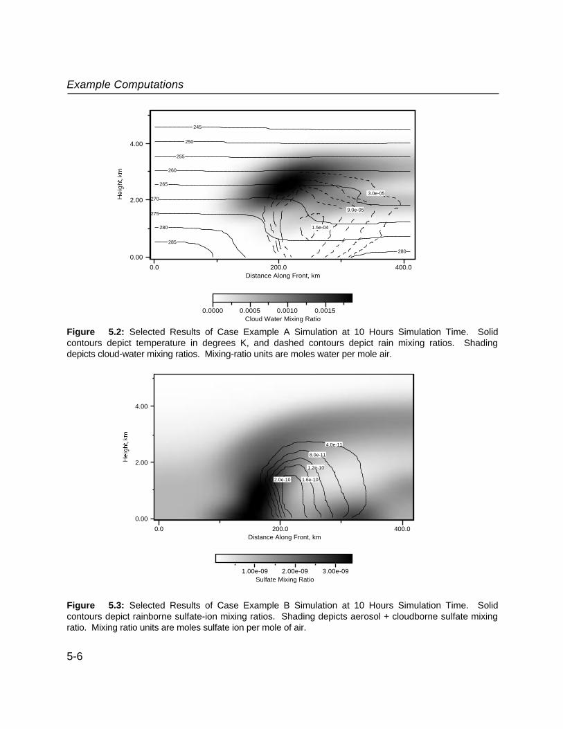
Because the intent of this user's manual is to instruct the user on operational aspectsrather than to provide an exhaustive listing of results, we shall limit the examples ofcomputed output here. Figure 5.2 shows selected meteorological fields computed bythe Case Example A simulation at ten hours simulation time. One should note that theonly transported variable shown here is rain. The others that appear in the figure(cloud water and temperature) are constrained variables, which are derived from thetransported variables water vapor and equivalent potential temperature (not shown inFigure 5.2).
Figure 5.3 shows selected chemical fields computed by the Case Example Bsimulation at ten hours simulation time. Here only two variables are shown: the sum ofsulfate aerosol and cloudborne sulfate ion, and rainborne sulfate ion. In contrast tothe situation for Figure 5.2, both of these are transported variables.
5-2

Example Computations
Table 5.1: Summary of Physicochemical Parameterizations Applied for Case-ExampleSimulations A and B
Interaction Parameterization
Cloud droplet autoconversion Berry-Reinhardt (1974) parameterization.*
Cloud droplet accretion Scott (1982) parameterization.*
Cloud droplet riming Scott (1982) parameterization.*
Vapor deposition to ice Easter-Hales (1984) parameterization.*
Raindrop evaporation Kessler (1969) parameterization.*
Raindrop freezing Lin et al. (1983) parameterization.*
Droplet nucleation (by both sulfate andnitrate particles)
Assumed first-order (in particle concentration) rate of 0.01sec-1 in updraft; zero otherwise.
Aerosol capture by rain (both sulfate andnitrate particles)
Based on scavenging-coefficient relationship, taken fromDana and Hales (1976).
Sulfur dioxide solubility in water Equations from Hales and Sutter (1973).
Ozone solubility in water Implicitly incorporated in rate relationship of Penkett et al.(1979).
Nitric acid solubility in water Relationship of Schwartz and White (1981).
Hydrogen peroxide solubility in water Relationship of Martin and Damschen (1981).
Ozone mass transfer to rain Solubility equilibrium assumed.
Sulfur dioxide, nitric acid, and hydrogenperoxide mass transfer to rain
Reversible mass transfer to raindrop ensemble;generalization of Froessling equation [Bird, et al., (1960)]
Ozone oxidation of S(IV) in cloud water Solubility equilibrium assumed for ozone and sulfurdioxide; Expression of Penkett et al. (1979) applied todescribe oxidation rate.
Hydrogen peroxide oxidation of S(IV) incloud water
Solubility equilibrium assumed for sulfur dioxide andreversible mass-transfer theory applied for hydrogenperoxide. Expression of Penkett et al. (1979) applied todescribe oxidation rate
Hydrogen peroxide oxidation of S(IV) inrain water
Reversible mass-transfer theory applied for both sulfurdioxide and hydrogen peroxide. Expression of Martin andDamschen (1981) applied to describe oxidation rate.
Hydrogen-ion concentration in cloudand rain water
[H+] = 1.03X10⁻⁵ + 1.18[SO42-] + 0.767[NO3-] (Based oncomposite behavior observed on the MAP3Sprecipitation-chemistry network [MAP3S (1982)].
*Cloud-physics treatment identical to that described by Easter and Hales (1984).
5-3

Example Computations
Table 5.2: Boundary Conditions Applied for Case-Example Simulations A and B
Dependent Variable Boundary Condition
Temperature (used to deriveθc)
Surface temperatures: 290°K on warm side and 282°K onthe cold side. Adiabatic profiles imposed.
Moisture (vapor + cloud water) 65%RH up to 2850 m on warm side and 45%RH on coldside; decreasing aloft as exp(20-z/150).
Sulfur dioxide + S(IV) in cloudwater
r(0) = 10 ppb. Flux computed by formulas 1 and 2.
Sulfate aerosol + sulfate incloud water
r(0) = 1 ppb. Flux computed by formulas 1 and 2.
Sulfate aerosol Computed above as for combined species. Cloud waterdoes not exist in inflow regions.
Nitric acid + nitrate in cloudwater
r(0) = 1 ppb. Flux computed by formulas 1 and 2.
Nitrate aerosol r(0) = 0.2 ppb. Flux computed by formulas 1 and 2.
Hydrogen peroxide r(z) = 1 ppb. Flux computed by formula 1.
Ozone r(z) = 50 ppb. Flux computed by formula 1.
Notes:All other dependent variables set to zero at inflow boundaries.Formula 1: Flux (z) = r(z)v(z)c where v(z) = local horizontal velocity.Formula 2: r(z) = r(0) between z = 0 and z = 1500 m; r(z) = r(0) exp[0.0001(1500-z) above z = 1500 m,
where r is the molar mixing ratio and r(0) is its value at z = 0.
5.2 Executing the Case Example Codes
To reproduce the Case Example A and B simulations, the user should apply thefollowing procedure:
1. Compile and link the total code using versions of the include file pluvius.com andthe subroutines inptgn, init, cleanup, and gen that are appropriate to CaseExample A. These are listed in Tables 6.3a, 6.4a, 6.6a, 6.13a, and 6.43a.
5-4

Example Computations
2. Execute the resulting executable code to produce the output files diskoutpt anddiskbkup. (Upon execution, the user will observe screen output at each time-stepcorresponding to temperature and humidity data at grid index j=15, k=19. Thevariable diff represents the difference between the saturation humidity and thecomputed sum of vapor plus cloud water; it will approach zero as the local airbecomes saturated and go positive after cloud formation occurs. The printstatements producing this screen output are located in the main program pluviusand should be removed after the user gains sufficient confidence in the code.) Thecode will terminate at 10 hours simulation time (36000 seconds).
3. Use the meteorological fields contained in file diskoutpt to compare with those inFigure 5.2.
4. Prepare for the Case Example B simulation: Delete or rename file diskoutpt.Rename the binary file diskbkup (which was produced by the Case Example Asimulation) to diskbkup.exa, so that it will be recognized by the input subroutinecloudinit. Compile and link the total code using versions of the include filepluvius.com and the subroutines inptgn, init, cleanup, and gen that areappropriate to Case Example B. These are listed in Tables 6.3b, 6.4b, 6.6b,6.13b, and 6.43b.
5. Execute the resulting executable code to produce the new output file diskoutpt.
6. Use the chemical fields contained in file diskoutpt to compare with those inFigure 5.3.
The above operations are straightforward, and will require three to four hours tocomplete on a typical work station. Once these are completed successfully the usershould experiment with the code further by modifying various model elements, such asboundary conditions, chemical species, or physicochemical mechanisms.Subsequent to this the user should have sufficient confidence to make moresubstantial changes to the code and to apply it for more complex physical andchemical environments.
5-5
Example Computations
1.5e-04
9.0e-05
3.0e-05
280
245
250
255
260
265
270
275
280
285
0.0 200.0 400.0
4.00
2.00
0.00
Distance Along Front, km
Hei
ght,
km
0.0000 0.0005 0.0010 0.0015Cloud Water Mixing Ratio
Figure 5.2: Selected Results of Case Example A Simulation at 10 Hours Simulation Time. Solidcontours depict temperature in degrees K, and dashed contours depict rain mixing ratios. Shadingdepicts cloud-water mixing ratios. Mixing-ratio units are moles water per mole air.
4.0e-11
8.0e-11
1.2e-10
1.6e-102.0e-10
0.0 200.0 400.0
4.00
2.00
0.00
Distance Along Front, km
Hei
ght,
km
1.00e-09 2.00e-09 3.00e-09Sulfate Mixing Ratio
Figure 5.3: Selected Results of Case Example B Simulation at 10 Hours Simulation Time. Solidcontours depict rainborne sulfate-ion mixing ratios. Shading depicts aerosol + cloudborne sulfate mixingratio. Mixing ratio units are moles sulfate ion per mole of air.
5-6
Section 6
Detailed Code Description
6.1 Introduction
This section provides a detailed description of the Pluvius II code in a logicalprogression which follows, at various levels of depth, the code’s execution flow.Considerable amounts of material are presented here, and we recommend thatpersons unfamiliar with Pluvius II do not attempt to read through this section frombeginning to end in a completely linear fashion. We suggest, rather, that the newreader peruse down through the first few subroutines to get an initial idea of the logicalflow and of how input is submitted to the code, to the depth of the core subroutine thatcontrols the numerical integration sequence (named subroutine core, notsurprisingly). Following this initial perusal, the unfamiliar reader is advised toimmediately follow the procedure indicated in Section 5 to execute the demonstrationprogram on his or her own machine. Subsequently, the user can examine variousaspects of the code by making progressive changes in selected subroutines, such asmodifying wind fields, changing kinetics mechanisms and parameters, and so-forth,until sufficient confidence is acquired to move directly to the user’s intendedapplication. Definitions of the code's common-block variables are summarized inTable 6.1.
A few additional initial comments are helpful at this point. First, it is useful to note thatPluvius II’s preferred unit system is cgs, and that the code’s dependent variables(except for temperature) are normally expressed in terms of mixing ratios (molespollutant per mole of air). Other units are employed on occasion for internalexpediency, but this practice is limited inasmuch as is practical.
Second, the description given here follows the two Case Examples of this user’smanual, which were described previously in Section 5. While many of the code’ssubroutines are invariant with respect to any specific application, others are intendedto be modified by the user to fit specific purposes at-hand. Consequently, several ofthe subroutines appearing in the following pages are presented twice — once forCase Example A and once for Case Example B — and each subroutine is relegated toone of three classes as follows:
Class I Subroutines - Those subroutines that are essential for operation of thecode, but are intended for modular replacement by the user.
Class II Subroutines - Those subroutines that are essential for operation of thecode and in general should be left unchanged.
6-1
Detailed Code Description
Class III Subroutines - Those special-purpose subroutines, to be supplied by theuser, that are necessary only for the specific modelling purpose at hand.
This approach to the presentation is intended to provide the user with additionalinsight regarding further modifications of the code for his or her specific application.
6.2 Overview of Main Program and First-Level Subroutines
The code’s main program, pluvius, is shown in Table 6.2. As its internaldocumentation suggests, this main program first calls subroutine inptgn to define thevertical and horizontal grids as well as to read in control variables and all otherassociated input except for that pertaining to the code’s initial conditions. It then callssubroutine femset, which defines several arrays used for the finite-element transportintegrations. Subsequently the code sets the model's initial conditions (subroutineinit), and then performs an inflow/outflow material balance over the computationaldomain by first establishing the initial wind field (subroutine wind) and then callingsubroutine matbal. It should be noted in this context that execution of the material-balance subroutine is something of a bookkeeping exercise and is not an essentialactivity of the code; but overall material-balance information is often a highly desirableby-product of the base computations. During this initial process the code also writes todisk storage the initial concentration fields by calling subroutine printi.
Next, the execution proceeds to the code’s main computation loop. Subroutine windis called once again (this is redundant for the first pass through the loop, since thewind fields for this example are time-invariant and have been computed in theprevious call to wind. Typical versions of wind sense this redundant call under suchconditions and simply perform a no-action return). Diffusivities are then calculated foreach point in the computation domain (subroutine diff), and the execution proceedsto subroutine core which, as indicated above, orchestrates the numerical integrationprocess for one composite time-step.
Subroutine cleanup is then called. This subroutine corrects for the propensity of thenumerical methods called by subroutine core to produce small, but still nonzero,values of the dependent variables in regions where, by definition, values should beidentically equal to zero. A prime example of this is the region in clear air, whereresidual small values for the concentrations of chemical species in cloud water areoften generated by the code. These numbers are very small and thus pose no realproblem, but the output’s readability is enhanced significantly if they are replaced byzero values prior to printing.
6-2

Detailed Code Description
Depending on the print-control variables, the computed results may be written to diskfiles at this point. Typically two different disk files are written for this purpose. Theprimary disk file is named diskoutpt, assigned to unit 20, and created as an ASCIIfile by subroutine printi. It is intended for outputting the conventional computedresults of the code. A second disk file is named diskbkup, assigned to unit 21, andcreated as an unformatted file by subroutine collect. It contains all of those variablesthat would be necessary to restart the simulation at the current model time, t. Thisfile is used mainly for subsequently restarting the computations in the event of somesystem interrupt. Upon writing the appropriate results, subroutine matbal is calledagain to produce the material-balance values for the total computational domain. Atthis point — and provided the time-limit tstop has not been exceeded — the coderepeats the main computation loop for a subsequent time-step. If tstop has beenexceeded, the code executes a normal termination and concludes the active program.
In conclusion to this cursory overview of Pluvius II's main program, it should beemphasized that several of the first-level subroutines described here (inptgn, init,wind, printi, print, diff, cleanup, and matbal) are application-specific and thusare intended to be modified by the user. One should note also that most of the code’svariables are communicated between subroutines via common blocks in the includefile pluvius.com. The pluvius.com files for the two case examples described in thisuser’s manual are given in Tables 6.3a and 6.3b.
Versions of subroutine inptgn corresponding to Case Examples A and B are shown,respectively, in Tables 6.4a and 6.4b. In Case Example A the procedure is relativelystraightforward, with the pertinent information being entered via the subroutine in anessentially linear manner. First, the mtrans, mtrany, and mtranx variables are set fora two-dimensional execution, allowing transport calculations to be performed in thevertical- and y-directions only. Next a two-dimensional grid is established, whichcontains 31 and 35 grid points in the horizontal and vertical dimensions, respectively.
This Case-Example A simulation includes four transported variables (the sum of cloudwater and water vapor, rain, snow, and equivalent potential temperature) plus threeconstrained variables (cloud water, water vapor, and temperature), and the code isinformed of these quantities by setting the variables ltot and ltot2. Vapor andcloud water are treated as a single summed variable here for two reasons. First, thispractice eliminates abrupt discontinuities in the transported variables at the cloudboundaries; second, when equivalent potential temperature is used as an advectedthermodynamic variable, both water vapor and cloud water become constrained by thezero-supersaturation assumption.
6-3

Detailed Code Description
As noted previously, Pluvius II allows different transported variables to move indifferent fashions, depending on their physical properties; thus snow and rain, havingunique fall velocities, are allowed here to advect in individual "regimes," which in turnare different from those of the gaseous species and temperature. The total numbers oftransport regimes for a particular simulation are specified by the variables lpxtot,lpytot and lpstot. In this particular example four vertical (snow, rain, air, andtemperature) and two horizontal (air and temperature) transport regimes are specified.An individual regime is allocated here for temperature (heat transfer), presuming thatthe eddy diffusivity for this case may be different than that for the more convectivelypassive species.1
Next, integer index variables and alphanumeric species names are associated withthe numerical index-values for each of the transported and constrained variables. Theindex variables are primarily for recognition convenience when the indices are used inlater portions of the code. The alphanumeric species names, in combination with a runtitle which is also supplied at this point, are used in subsequent disk output ofcomputed results. An essential rule in the naming operation is that indices of thetransported variables must range from 1 to ltot and those of the constrainedvariables must range from ltot + 1 to ltot2; otherwise, species indices may be setin a totally arbitrary manner. Transport-regime indices are then assigned to the arrayslprops and lpropy.
Next, the code's output controls are established (the subroutine restart is bypassedin this Case Example). nprint is set to write to a primary disk file after every 480composite integration time-steps (every 7200 seconds). itdisk is set to write updatedrecords to a second, backup disk file, erasing the previous record upon activation.tdisk and dtdisk are set to start writing the backup records after one hour ofsimulation time and to repeat every hour thereafter.
Following this, the code's primary temporal and spatial grid-spacing parameters areestablished. The simulation's start time is initialized to zero, the advective time-stepsare set to 7.5 seconds, and the simulation time limit is set at ten hours. dsunif anddyunif establish the z and y grid spacings in centimeters and instruct the code toapply uniform vertical and horizontal grid spacings, and scord(1) and ycord(1) set thelower positions of the computational grid to zero. Next, subroutine grdxyz, shown inTable 6.19, is called to set up the computation grid. For uniform-grid conditions grdxyzsimply sets the arrays xcord, ycord, and/or scord as appropriate, and returns tosubroutine inptgn. If a nonuniform grid is indeed desired, then grid data in the form
1The diffusivity fields used for heat and mass transfer are identical in Case Example A . The extra regimeprovided here is simply illustrate the availability of this option, if different diffusivity fields are desired.
6-4
Detailed Code Description
of xcord, ycord, and/or scord arrays should be entered explicitly through subroutineinptgn prior to the call to grdxyz.
Next, subroutine inptgn proceeds to identify control variables for execution of theordinary differential-equation (ODE) integrator odeint. These variables are specific tothis particular integrator, and must be appropriately replaced if an alternate integratoris applied. eps sets an error limit for the ODE code, and dtmin establishes thesmallest time-increment allowed before the code exits with an error return. ncorr andiexp are set, respectively, so that a single correction pass is applied in the code'spredictor-corrector cycle, and true exponentials (as opposed to Taylor's-seriesapproximations) are applied to simulate species decay rates. ratesf and cminestablish, respectively, the species decay rates beyond which stiff ODE calculationsare applied and the concentrations below which the associated variables areconsidered identically equal to zero. cerror is an array containing values of thedependent variables below which relaxed convergence criteria are applied. Most ofthese variables can be considered tuning parameters which are employed to optimizeperformance of odeint. The ones given here result in acceptable code operation forpresent purposes, but the user can adjust these as he or she feels appropriate.
Several of the following variables are obvious from the code listing. The boundaryconditions are set to flux-specified types by setting the lower and upper boundary-condition specifier variables to unity for each of the transported species. Thesubroutine frequency variables are set so that transport properties are updated witheach advective time-step and several control-toggle variables are set: mgen = 1 setsthe code so that its ODE portion is operative; mtemp = 1 instructs the code to includean energy balance as part of its calculation; and nonsym = -1 tells the core subroutineto operate in its normal, "symmetric" operational mode.
Next, subroutine inptgn sets the control parameters for the code's filtering scheme,which is used to reduce high-frequency noise produced by the numerical integrationprocess. Without going into large detail at this point, nfilts and nfilty define thenumber of advective time steps prior to each filter application in the respectivedirections. nfilsrch, nfiltset, and nfiltitr are internal parameters used by thefiltering scheme, and filfacs is an array describing the degree of filtering for eachtransported species ( these should be set to 0.0 for no filtering whatsoever). Furtherinformation on Pluvius II's filtering scheme can be acquired from the listing forsubroutine foresfilt, which is given in Table 6.40 and by referring to Forester(1977). The final operation of subroutine inptgn is to turn off the boundary filter for thex-direction, and to turn on its counterparts for the vertical- and y-directions. Setting thelast two variables to unity activates additional filtering of results in the boundaryregions.
6-5

Detailed Code Description
The structure of subroutine inptgn for Case Example B is quite similar to that for CaseExample A. As with lvapcl in Case Example A, some of the transported chemicalspecies have been summed for computational convenience; thus lso2gcl representsthe sulfur dioxide that occurs in the gas phase plus that which is dissolved in localcloud water, and the remaining variables take on their obvious significances(constrained variables lhcloud and lhrain pertain respectively to the hydrogen-ioncontent of cloud- and rain-water, and are calculated simply from an ion balance).Case Example B includes 15 transported species (ending with gas-phase ozone).The variables such as lrain, lsnow, and lvapcl are now relegated to "constrained"status, since they are specified here from the results of Case Example A and are notcomputed as a part of Case Example B's numerical-integration scheme.
Final portions of this inptgn version are straightforward extensions of that in CaseExample A. The only feature that deserves some additional comment in this context isthe transport-regime designation for the various chemical species, noting thatchemicals associated with falling rain and snow inherit the terminal fall speeds ofthese meteorological entities, and thus are assigned the associated values of lprops.
Subroutine femset, which establishes key grid-related parameters for the finite-element integration, is shown in Table 6.5. The first task performed by this subroutineis to zero a number of the finite-element integration parameters, having the variousvariable names ct__(idum,i), where the index idum pertains to dimension x, y, or z(1,2, or 3, respectively) and i is the associated grid index. It then computes theassociated values of the finite-element integration parameters for all dimensions thatare active in the simulation.
Subroutine init assumes final responsibility for establishing the initial conditions forthe transported variables r(i,j,k,l) for the total computational domain. For CaseExample A, this involves stipulating surface pressures and temperatures for the warmand cold sectors, deriving temperature and humidity profiles for associated aircolumns on the basis of adiabatic lapse rates and specified relative humidities, andthen applying these profiles to warm- and cold-sector portions of the computationaldomain. The code in Table 6.6a begins to the left of the front, in the warm-sector air,and stipulates a surface temperature of 290 °K for this region. Next it computes acorresponding air concentration using an equation of state and sets a water-vapormixing ratio that is 65 percent of its saturation value (here sat is an internal functionthat returns a concentration of water vapor in saturated air, when supplied the localabsolute temperature).
6-6
Detailed Code Description
Following these and some additional bookkeeping steps, the code estimates theconcentration of air at points aloft using an approximate hydrostatic equation. Theresulting air concentrations then are applied to compute temperatures aloft, which inturn are used to set water-vapor mixing ratios such that relative humidities are 65% upto the 20th grid point and decrease aloft. Subsequently, these initial temperature,pressure, mixing-ratio, and concentration profiles are applied to all internal grid points.
This general procedure is then applied for cold-sector air to the right of the front. Here,however, the surface temperature is set to 282 °K and the relative humidity is set at 45percent. The associated temperature, pressure, mixing ratio, and concentrationprofiles are subsequently "painted" into the cold-wedge region below the frontalsurface, resulting in a temperature and humidity discontinuity across the front.
One should note that no clouds occur in this initial environment, and that we shouldexpect clouds to emerge in the simulation as the moist air moves upward over thefrontal surface. Also one should note that, since the code's execution will progress tosimulation times that are sufficient to render the system essentially boundary-conditionlimited, any reasonable set of initial conditions would suffice for present purposes: theones described here were chosen simply because they give an uncomplicated butreasonable representation of behavior, which is sufficient for initiating thecomputational process.
After initial conditions have been set, subroutine inflowinit is called, which storesinitial boundary concentrations for the subsequent calculation of inflow boundaryconditions. The final action of subroutine init is to call subroutine restart if initmodespecifies a restart from a previous backup disk file. As noted in the documentation, thecurrent version of inflowinit is intended for time-invariant boundary conditions only,and the user should modify (or possibly eliminate) this subroutine if time-variantboundary conditions are imposed.
The version of subroutine init for Case Example B is simpler than its Case Example Acounterpart, mainly because the meteorological variables have been preset by CaseExample A's execution, and need only to be copied here. This operation is performedby calling subroutine cloudinit, which reads the unformatted disk file that was writtenby the Case Example A execution and subsequently renamed diskoutpt.exa.
The Case Example B initial conditions for the chemical variables have been chosen tobe rather simple in form: constant mixing ratios up to 1500 meters and decreasingaloft, except for hydrogen peroxide and ozone. As with Case Example A, we expectthis chemical system to be boundary-condition limited at large simulation times; thusany reasonable set of initial conditions should suffice here as well.
6-7

Detailed Code Description
Subroutine wind establishes numerical values for the x, y, and z components of themodel's wind fields. The example of subroutine wind given in Table 6.7 sets the two-dimensional wind field used for the two-dimensional Case Examples A and B. Sincethese examples apply a wind field that is fixed in time, the code appearing in Table 6.7implements an immediate no-action return after its initial interrogation.
The wind field described by this subroutine version corresponds to the vertical slice ofan idealized warm-frontal system that was shown in Figure 5.1. Winds within thisscheme are relative to the motion of a warm-frontal surface, which progresses from leftto right, with air from the warm-frontal zone moving to the right and upward over thefrontal surface. Cold air at low elevations below the frontal surface moves to the left(relative to the front), ascends, and then reverses direction at higher altitudes.
The subroutine calculates mass-consistent wind fields for four specific zones of Figure5.1. The first of these is to the left of the surface front: here the vertical velocities arezero, and the horizontal velocities scale with air density (for mass-consistency) in astraightforward manner. The second zone occurs in the region above the ascendingwarm front. Here vertical velocities in the vicinity of the frontal surface correspond tomovement over this surface, and fall to zero at the top of the model domain. Again, thecode adjusts the horizontal winds to achieve mass consistency in reflection of theprescribed vertical motions.
The third zone is the cold-air wedge underlying the cold front. This portion of the fieldis calculated by allowing the horizontal winds immediately below the frontal surface tohave horizontal and vertical components which are identical to those of the airimmediately above the front, and then computing material fluxes at lower grid pointsnecessary to maintain mass-continuity in this region. Finally, velocity components forthe fourth zone (the air immediately to the right of the front) are computed in a mannerthat preserves mass consistency and harmony with the wind-fields in the adjoiningfrontal region.
The code’s utility printing subroutines, printi and print, are listed in Tables 6.8 and6.9, respectively. As can be noted from the main pluvius code in Table 6.2, printi iscalled once only, and is intended to output any code diagnostics (to file diagnostics)and the initial concentration and temperature fields (to file diskoutpt, which isintended for subsequent use in outputting corresponding fields computed at futuresimulation times).
Subroutine print is quite similar to printi. In contrast to the initial printing routine,however, this subroutine does not open the output files (since they have been openedpreviously). The examples of printi and print shown here have been used to
6-8

Detailed Code Description
output the primary numerical results for Case Examples A and B. Since the desiredoutput formats will be strongly dependent on the modeling application at-hand, bothprinti and print are intended for modification by the user.
As noted above, subroutine matbal (Table 6.10) is essentially a bookkeeping routine,which performs integral material balances over the computational domain todetermine advective inflow/outflow rates and material fluxes. matbal's basicapproach is to operate sequentially on the domain's left-hand, right-hand, and thenbottom boundaries. At each boundary it computes advective fluxes at all appropriategrid points, integrates these spatially to obtain total material-balance components, andthen prints the resulting data to disk. Subroutine integrate is a simple quadratureroutine which is applied for this purpose. In the case of the lower boundary, thevertical fluxes are computed from the vertical transport velocities, which result fromsedimentation of the pollutant-containing precipitation. These velocities are calculatedusing subroutine transport, and are stored in the array vertcclm. One should notehere that snow does not reach the ground in this simulation and that dry deposition isignored; thus the only deposition mechanism is through rainfall. The subroutineshould be modified by the user in situations where these conditions are not met. Oneshould note here again that subroutine matbal is not necessary for execution of thePluvius II code, and can be deleted from the main program, if desired.
Subroutine diff, shown in Table 6.11, sets diffusivities for each transport regime ateach grid point of the computational domain. The very simple example shown hereestablishes all diffusivities at 105 cm2/s. Since these are held constant with time, thisversion of subroutine diff executes a no-action return after its initial interrogation.
Subroutine core, shown in Table 6.12, is in many respects the heart of the Pluvius IIcode. In a typical execution this routine solves equation (3.2) for a double timeincrement 2∆t, in the sequence indicated by that equation:
∆ζ total,2∆t
= ∆ζ x,∆t
+ ∆ζ y,∆t
+ ∆ζ z,∆t
+ ∆ζ transformation,2∆t
+ ∆ζ z,∆t
+ ∆ζ y,∆t
+ ∆ζ x,∆t . (3.2)
In the event that the x- and or y-dimensions are inactive in a particular simulation, thecode simply bypasses the corresponding steps. Pluvius II also gives the option ofproceeding through equation (3.2) halfway, and thus computing for a single time-increment ∆t. This option is controlled via the toggle-variable nonsym, as indicated inthe code listing.
6-9
Detailed Code Description
Subroutine coreOO, shown in Table 6.18, is called only on the first execution ofsubroutine core. It computes physical-property related variables which are time-invariant, and thus need to be computed only once during the simulation. Afterpassing this point, the code next executes initial integrations for a single time-step inthe x- and y-directions (as appropriate to the problem at-hand), calling the integrationroutines xinteg and yinteg. It is important to note in this context that a singleinterrogation of each of these subroutines results in integrations for all ltottransported species.
Subsequent to these operations, the code proceeds to the vertical-integration stage,where the process is somewhat more complicated for two reasons. First, and asmentioned previously, the current code version segregates vertical integrationoperations on a column-by-column basis. Within this operation, transported variablesand pertinent other parameters are "packed" into special one-dimensional arrays byexecuting the subroutine ijpack, which is exhibited in Table 6.55. The secondcomplication results from the frequent need, when precipitation exists, to reduce thetime-step for vertical integration in order to preserve Courant-number stability. This isdone by calling subroutine sbstep, which returns the (possibly) modified timeincrement dtsub. The listing for subroutine sbstep is shown in Table 6.54.
Upon accomplishing these initial steps for the vertical integration, subroutine coreproceeds to process multiple dtsub increments, performing the operations
∆ζ z,dtsub
+ ∆ζ transformation,2dtsub
+ ∆ζ z,dtsub
repeatedly, until a full double increment 2∆t is traversed. Subroutines sinteg andchmint respectively coordinate individual integrations for the vertical dimension and fortransformation. Upon completing this full cycle for all i,j columns, the code callssubroutine sfilter to conduct some required bookkeeping operations, and convertsthe columnized data back to its original r(i,j,k,l) configuration by calling subroutineijunpack. A listing of ijunpack is given in Table 6.56.
Finally (and if symmetric integrations are desired), the code conducts furtherintegrations for a single time-step in the x- and y-directions, again calling theintegration routines xinteg and yinteg.
Versions of subroutine cleanup corresponding to Case Examples A and B are shownin Tables 6.13a and 6.13b, respectively. These subroutines zero-out variables underconditions where concentrations should be identically equal to zero, and also computevalues of constrained variables as appropriate.
6-10
Detailed Code Description
The computational procedures are generally obvious from the code listings, and thuslittle comment is necessary at this point. In the Case Example A version, temperature(a constrained variable) is calculated from the equivalent potential temperature (atransported variable) using subroutine tfrmth, which is listed in Table 6.51.
Subroutine collect, shown in Table 6.14, combines with printi, matbal, and printto provide an additional data-output utility. In contrast to printi and print, however,this subroutine is intended to log current computed results for the event that the usermay desire to restart the code at an advanced time, subsequent to previoussimulations. This convenience can be helpful under the contingency conditions of asystem crash, or if the user desires to extend a simulation or perform it in pieces.
As can be noted from the code, the salient output data are written in unformatted formon disk file diskbkup. Through the control variables itdisk, tdisk, and dtdisk theuser has the choice to record sequential time-frames of data, only the final time frame,or none at all. Subroutine collect is intended to serve as a generic subroutine andgenerally does not require modification by the user.
6.3 Overview of Second- and Lower-Level Subroutines
This subsection presents all of those subroutines within the Pluvius II code that are notcalled directly by the main program. In this presentation we shall attempt to follow alogical flow, starting with those subroutines mentioned in the above discussion, andproceeding through the total set in a manner that approximates the flow of theprogram's execution.
6.3.1 Initialization and Grid-Setup Operations
Subroutine restart, shown in Table 6.15, is responsible for reading the disk outputgenerated by subroutine collect. This listing essentially mirrors that of subroutinecollect. One should note here that subroutine restart is not used in the two caseexamples presented here. Rather, the file generated by subroutine collect in CaseExample A is read in Case Example B by cloudinit, (Table 6.16) which was written asan ad hoc subroutine for this special purpose.
As noted above, subroutine inflowinit (Table 6.17) is called from subroutine init topreserve boundary concentrations for possible later use in computing fluxes for inflowboundary conditions. Also as noted above, subroutine coreOO (Table 6.18) is calledfrom subroutine core (Table 6.12) once only, on the initial call to core. coreOO
6-11
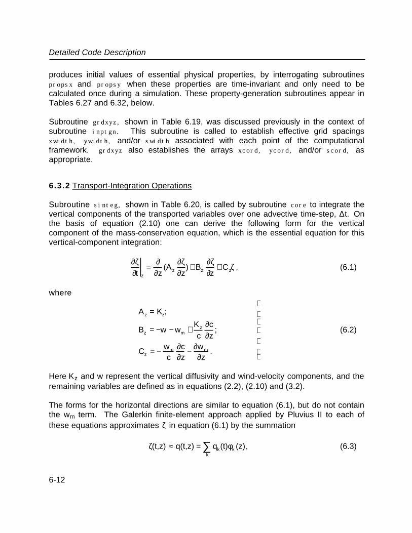
Detailed Code Description
produces initial values of essential physical properties, by interrogating subroutinespropsx and propsy when these properties are time-invariant and only need to becalculated once during a simulation. These property-generation subroutines appear inTables 6.27 and 6.32, below.
Subroutine grdxyz, shown in Table 6.19, was discussed previously in the context ofsubroutine inptgn. This subroutine is called to establish effective grid spacingsxwidth, ywidth, and/or swidth associated with each point of the computationalframework. grdxyz also establishes the arrays xcord, ycord, and/or scord, asappropriate.
6.3.2 Transport-Integration Operations
Subroutine sinteg, shown in Table 6.20, is called by subroutine core to integrate thevertical components of the transported variables over one advective time-step, ∆t. Onthe basis of equation (2.10) one can derive the following form for the verticalcomponent of the mass-conservation equation, which is the essential equation for thisvertical-component integration:
∂ζ∂t z
=∂
∂z(Az
∂ζ∂z
) + Bz
∂ζ∂z
+ Czζ , (6.1)
where
Az = Kz;
Bz = −w − wm +Kz
c∂c∂z
;
Cz = − wm
c∂c∂z
− ∂wm
∂z.
(6.2)
Here Kz and w represent the vertical diffusivity and wind-velocity components, and theremaining variables are defined as in equations (2.2), (2.10) and (3.2).
The forms for the horizontal directions are similar to equation (6.1), but do not containthe wm term. The Galerkin finite-element approach applied by Pluvius II to each ofthese equations approximates ζ in equation (6.1) by the summation
ζ(t,z) ≈ q(t,z) = qk(t)φk (z)k
∑ , (6.3)
6-12

Detailed Code Description
where the qk are the values of the approximation q at each grid-point k and the "basisfunctions" φ k are linear functions that have values of unity at the grid points zk, zero atimmediate neighbor points, and zero at all locations beyond the immediate neighbors:
φk(z) =
0 for z ≤ zk-1 and z ≥ zk+1
z -z k-1
zk − zk −1
for zk-1 ≤ z ≤ zk
z-z k+1
zk − zk +1
for zk ≤ z ≤ zk +1
(6.4)
The spatial discretization of equation (6.1) is obtained by requiring that
φk(z)∂q∂t
−∂
∂z(Az
∂q∂z
) −Bz
∂q∂z
− Czq
∫ dz = 0 (6.5)
for all k, where the integration limits correspond to the extent of the z-domain andwhere the coefficients Az, Bz, and Cz as well as q are represented in terms of basis-function expansions. Evaluation of equation (6.5) is straightforward because of thesimple form of φ k and yields
f k
∂qk−1
∂t+ gk
∂qk
∂t+hk
∂qk +1
∂t= αkqk−1 + βkqk + γkqk+ 1 (6.6)
where αk, βk, and γ k depend on Az, Bz, and Cz and thus are time-dependent, while fk,gk, and hk depend only on the vertical grid spacing.
Crank-Nicholson time discretization is now applied to equation (6.6). Terms on theleft-hand side are approximated as
∂qk
∂t≈
qk* − ˜ q k∆t
(6.7)
where qk* = qk(t +∆t) and ˜ q k = qk(t) . Terms on the right-hand side are approximated as
6-13

Detailed Code Description
βkqk ≈ 0.5˜ β k(qk* + ˜ q k ). (6.8)
Combined with equations (6.6) and (6.7), this gives the following set of linearequations, which has a tridiagonal coefficient matrix:
qk −1
* ( ˜ α k −2∆t
fk) + qk* ( ˜ β k −
2∆t
gk ) + qk +1* ( ˜ γ k −
2∆t
hk ) =
˜ q k− 1(− ˜ α k −2∆t
fk) + ˜ q k (−˜ β k −2∆t
gk ) + ˜ q k− 1(−˜ γ k −2∆t
hk ). (6.9)
Pluvius II's vertical transport-integration subroutines perform the following tasks:Subroutine sinteg (Table 6.20) performs a general coordination of the verticalintegration process. Subroutine propss (Table 6.21) computes values of Az, Bz, andCz for the grid locations zk at the current model time and stores them in the arrays aas,bbs, and ccs, respectively.2 Subroutine coefss (Table 6.22) uses these arrays to
compute the ˜ α k , ˜ β k , and ˜ γ k, and subsequently the coefficients on the left-hand side ofequation (6.9). These values are also stored in aas, bbs, and ccs, thus overwritingAz, Bz, and Cz, which are no longer needed. Subroutine bounds (Table 6.23) setsappropriate coefficients at the top and bottom extremities of the solution vector.Subroutine loads (Table 6.24) transfers the appropriate sets of aas, bbs, and ccs tothe arrays a, b, and c. In addition, it computes the right-hand side of equation (6.9)and stores this in the d array. Arrays a, b, c, and d are used directly by subroutinetridag to solve the set of linear equations for the values of qk
* (the numericalapproximations to ζk at time t + ∆t), which are returned in the array v.
In contrast to subroutines sinteg, propss, coeffs, bounds, and loads, subroutinetransport is application-specific and is intended for modification by the user. Theexample shown in Table 6.25 calculates rain and snow fall velocities usingparameterizations described earlier by Easter and Hales (1984), and also estimatesprecipitation spread parameters associated with differential settling velocities ofdifferent-size hydrometeors. These spread parameters are treated as conventionaldiffusivities and added to those associated with local air motions.
Numerical integration routines for the x-dimension (xinteg, propsx, coefsx, boundx,and loadx, shown in Tables 6.26 through 6.30, respectively) and for the y-dimension(yinteg, propsy, coefsy, boundy, and loady, shown in Tables 6.31 through 6.35,
2Note that a separate set of aas, bbs, and ccs is required for each transportregime.
6-14
Detailed Code Description
respectively) proceed through pathways that are similar to those for their vertical-integration counterparts. Because of this they will not be discussed further here,except to note that these routines are somewhat simpler than those for the verticalcomputations. Fewer physical terms are necessary in these horizontal computations,and they deal directly with the dependent variables r(i,j,k,l) rather than using their"columized" counterparts.
6.3.3 Numerical Filtering Operations
Filtering of short-wavelength numerical noise, which is generated by the finite-elementprocedure under conditions where advection dominates as a transport process, occursthrough calls to subroutines sfilter, xfilter, and yfilter, (Tables 6.36 through6.38) which in turn interrogate subroutines bndfilt and foresfilt, which are shownin Tables 6.39 and 6.40. Subroutines sfilter, xfilter, and yfilter determinewhether filtering is to be applied at the current stage in the computation and, if so,execute the subroutine calls to bndfilt and foresfilt, which perform the actualfiltering operations for the domain boundaries and internal grid-points, respectively.
As indicated by the listing in Table 6.39, subroutine bndfilt performs filteringoperations only under conditions where boundary inflow occurs, and only when flowconditions exceed specific levels, as determined by the local Peclet number, (vi ∆xi/Ki,where the subscript i denotes any appropriate dimension, x, y, or s). Subroutineforesfilt is based on a subroutine in the Pluvius Mod. 5 code (Easter and Hales1985), which applies the nonlinear filtering scheme suggested by Forester (1977).The reader is referred to these two references for more extensive discussion on thissubject.
6.3.4 Transformation-Integration Operations
Integration of the transformation terms associated with equation (3.2) is coordinatedthrough subroutine chmint, which is listed in Table 6.41. Because it is moreconvenient under most circumstances to compute transformation rates in terms ofabsolute concentrations, the first action of this subroutine is to convert the mixing ratiosin the rclm arrays to concentrations (in moles per cubic centimeter), and store thesevalues in the array cnn(l), where l is the species index. In the special case wherethe energy balance is calculated and l corresponds to the equivalent potentialtemperature, θc, these values are converted to actual temperatures (degrees Kelvin)by calling the subroutine tfrmth (cnn(ltheta) will contain the actual temperatureunder these circumstances).
6-15

Detailed Code Description
Upon performing these initial operations, chmint loads a first-guess of the optimumstep size for the transformation integration into dtsug. This value is set to zero if noprior integrations have occurred for that particular grid point, and is determined fromthe previous integration otherwise. The code subsequently calls subroutine odeint,which performs the actual numerical integration over the period dtchem, and thenstores the current value of dtsug in the array dtsave for possible later use. Upon asuccessful call to odeint, chmint restores the concentrations and potentialtemperature into the rclm array, and proceeds to the next grid point in the column.After processing an entire column the code returns to the calling subroutine core forsubsequent integration of the transport components.
As noted in Section 3.3, subroutine odeint, listed in Table 6.42, is only one of severalODE solvers that can be incorporated with Pluvius II to perform integrations of themodel's transformation terms, and the user may replace this routine without too muchtrouble, if desired. odeint is called by subroutine chmint giving the grid-point location(i,j,k), the starting time for the integration (tstrto), the total integration period forthat call (dttot), the suggested initial step-size (dtsug), and the maximum allowablestep size (dtmax) as arguments. Additional parameters are passed via commonblocks (see commenting at the start of the listing in Table 6.42). Primary output fromodeint is the vector of species concentrations cnn(l) resulting from the integrationprocess.
This particular odeint version is a somewhat modernized copy of the code given byEaster and Hales (1984). In essence it is a two-step, low-order, predictor-correctorscheme which has the ability to sense for stiff conditions. Under circumstancesinvolving stiff equations, the scheme shifts to an operation mode where species decayrates are approximated by exponential functions, thus preventing negative undershootand preserving stability at reasonably large step-sizes.
To implement this, odeint demands that rate expressions for species generation besegregated from their species-decay counterparts. This is accomplished using thearrays ggen(l) and gdec(l), which contain current rates in moles/cm3 sec and arecomputed by calls to subroutine gen, which is a user-supplied subroutine. Moredetailed information on odeint is available in the Easter-Hales reference, and the codeappearing in Table 6.42 is extensively documented to facillitate its application.
Examples of subroutine gen, corresponding to Case Example A and Case Example B,are given in Tables 6.43a and 6.43b, respectively. gen is called by subroutine odeint,giving the grid-point location (i,j,k), the current simulation time (tgen), and thecurrent odeint step-size (dtau). In addition, the argument list contains a flag (jpasso)to indicate whether the current odeint call is from the predictor or corrector pass.
6-16

Detailed Code Description
Primary output from gen consists of the vectors of generation and decay rates, as wellas species concentrations associated with selected constrained variables. As noted inthe context of subroutines inptgn and init, Case Example A involves four transportedvariables: equivalent potential temperature, vapor plus cloud water, rain, and snow.The code in Table 6.43a computes the associated generation and decay rates alongthe lines of the interaction diagram in Figure 4.1a, using cloud-physicsparameterizations described previously by Easter and Hales (1984) and summarizedin Table 5.1. The final portion of the subroutine computes corresponding terms of theenergy-balance equation, using the derived phase-transformation rates in conjunctionwith thermodynamic properties, as indicated by the right-hand side of equation (2.9).
The version of subroutine gen corresponding to Case Example B, shown in Table6.43b, performs operations that are similar to its Case Example A counterpart, butcorrespond to the chemical interaction diagrams in Figures 4.1b and 4.1c. Here itshould be noted that noted that the transfer of sulfur and nitrogen compounds betweenphysical media depends directly on the cloud-physics processes altering thesephases, and so many of the cloud-physics parameters must be computed in thisapplication as well. These operations are performed in the first major segment of thecode, which terminates just prior to statement number 1OO.
Following the cloud-physics computations, the code proceeds to establish currentconcentrations of the constrained species, and then moves immediately to calculatethe ggen and gdec arrays for the transported variables. Since the energy-balancecomponent of Pluvius II is inactive for Case Examble B, no latent-heating computationsare necessary for this version of gen. As was the case with Table 6.43a, thecalculations exhibited in Table 6.43b are derived mainly from those presented byEaster and Hales (1984) and summarized in Table 5.1, and the reader is referred tothese sources for additional information.
6.3.5 Utility Routines for Calculation of Thermodynamic Properties
Various utility subroutines and internal functions for calculating thermodynamicrelationships are listed in Tables 6.44 through 6.51. With few exceptions theseroutines are self-explanatory, and little elaboration will be given here. Subroutinehenry, listed in Table 6.50, is based on SO2 solubility equations described earlier byHales and Sutter (1973), and the reader can consult this reference if more informationis necessary.
Subroutine tfrmth, listed in Table 6.51 is used to convert from equivalent potentialtemperature to actual temperature whenever temperatures are required to evaluatethermodynamic and/or kinetic parameters. Calculations in this subroutine are basedon equations (2.7) and (2.8)
6-17

Detailed Code Description
θc = θd (1−
λcrcCpT
), (2.7)
θd = T(
1000 mbp
)R/Cp
, (2.8)
which were discussed previously in Section 2. Because the cloud-water mixing ratiorc is a constrained variable, its numerical value is generally unknown until T is known.This effectively renders T an implicit function of θc, and necessitates an iterative orinterpolative technique for calculating temperature. The code in Table 6.51 follows aninterpolative approach, using the base data points as described in the code listing.
6.3.6 General Utility Subroutines
Tables 6.52 through 6.56 are listings of miscelaneous utility subroutines. Subroutineintegrate, listed in Table 6.52 is a straightforward Simpson's-rule application, whichis used in this code exclusively to integrate fluxes in subroutine matbal to determineoverall inflow and outflow rates. It is nothing fancy, but is relatively efficient andsuffices for the purpose at hand. Subroutine tridag, listed in Table 6.53, is thetridiagonal matrix solver called by subroutines sinteg, xinegt, and yinteg, and hasbeen taken directly from the textbook of Carnahan, Luther, and Wilkes (1969).
Subroutine sbstep (Table 6.54) is called from the vertical-integration loop withinsubroutine core to determine appropriate time-substeps for the associated integrationprocess. As noted previously, this determination is based on a Courant-numbercriterion.
The final two subroutines in the code, ijpack and ijunpack are shown in Tables 6.55and 6.56. As noted previously, these routines are executed in conjunction with thevertical-integration step as a method for reducing page-faulting in computers wherecore memory resources are limited. ijpack moves key variables from their higher-dimensional arrays into lower-dimensional counterparts representing vertical columnsat specified x and y locations. For the dependent variables (in the r and rclm arrays), italso moves the updated rclm values from the last sinteg and chmint integrations backinto the r array. ijunpack performs a clean-up activity, moving updated rclm valuesfor the final column (i = itot, j = jtot) back into the r array.
Table 6.57 provides a summary of the total ensemble of Pluvius subroutines. This isintended primarily for the user's convenience as a locator for the various componentsof code discussed in this section.
6-18

Detailed Code Description
Table 6.1 Pluvius II Code Variable and Array Definitions
Variable Name Descriptiona Working array for tridiagonal matrix solution routine.aas Working array in vertical finite-element integration scheme.aax Working array in x-direction finite-element integration scheme.aay Working array in y-direction finite-element integration scheme.asofhi Working array in vertical finite-element integration scheme.
holds values of aas (as defined in propss) at lower boundary,k=1.
asoflo Working array in vertical finite-element integration scheme.holds values of aas (as defined in propss) at upper boundary,k=ktot.
axofhi Similar to asofhi, but for x-direction.axoflo Similar to asoflo, but for x-direction.ayofhi Similar to asofhi, but for y-direction.ayoflo Similar to asoflo, but for y-direction.ak glc/cp.alocp heatc/cp.b Working array for tridiagonal matrix solution routine.bbs Working array in vertical finite-element integration scheme.bbx Working array in x-direction finite-element integration scheme.bby Working array in y-direction finite-element integration scheme.bsofhi Working array in vertical finite-element integration scheme.
holds values of bbs (as defined in propss) at lower boundary,k=1.
bsoflo Working array in vertical finite-element integration scheme.holds values of bbs (as defined in propss) at upper boundary,k=ktot.
bxofhi Similar to bsofhi, but for x-direction.bxoflo Similar to bsoflo, but for x-direction.byofhi Similar to bsofhi, but for y-direction.byoflo Similar to bsoflo, but for y-direction.c Working array for tridiagonal matrix solution routine.cair Array containing molar air concentrations at grid points.cairclm Array holding molar air concentrations for current vertical
column of grid points during vertical transport andtransformation integrations.
ccs Working array in vertical finite-element integration scheme.ccx Working array in x-direction finite-element integration scheme.ccy Working array in y-direction finite-element integration scheme.
6-19
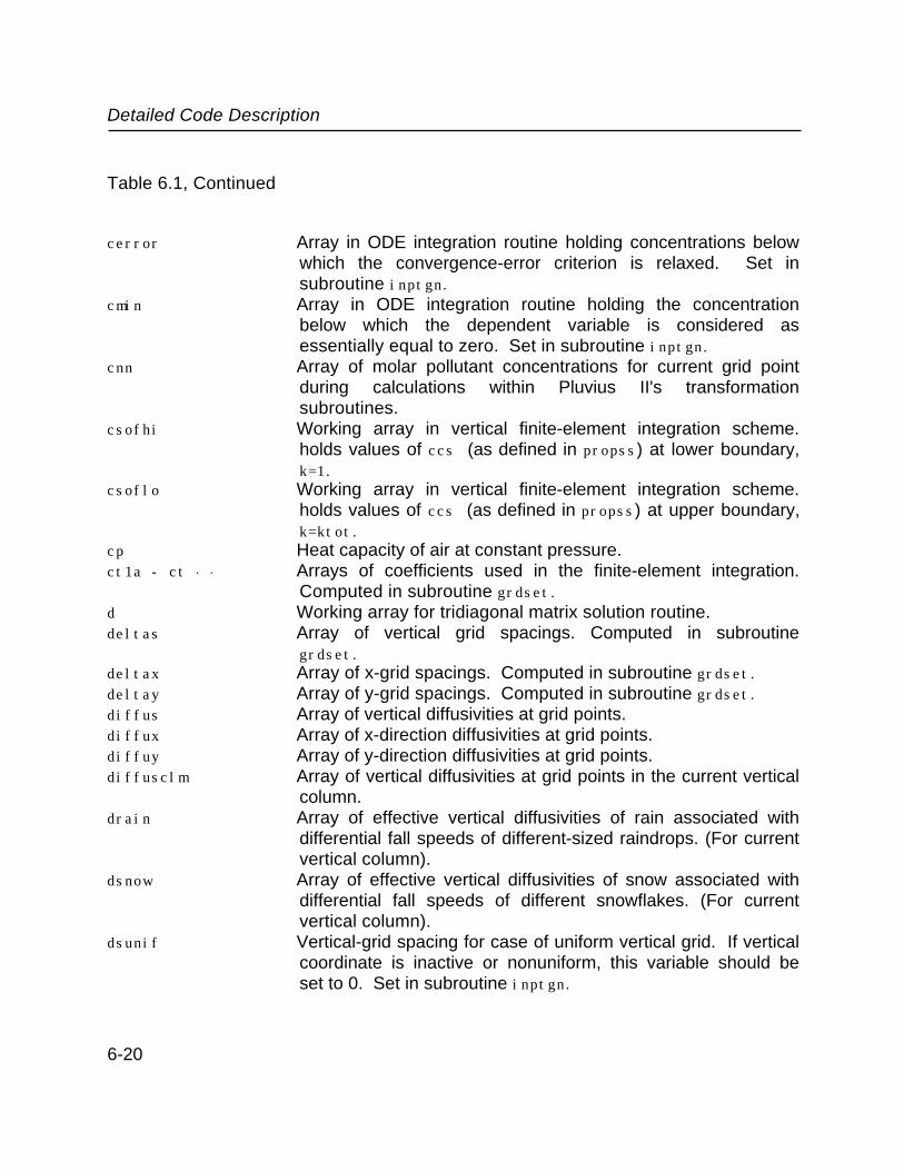
Detailed Code Description
Table 6.1, Continued
cerror Array in ODE integration routine holding concentrations belowwhich the convergence-error criterion is relaxed. Set insubroutine inptgn.
cmin Array in ODE integration routine holding the concentrationbelow which the dependent variable is considered asessentially equal to zero. Set in subroutine inptgn.
cnn Array of molar pollutant concentrations for current grid pointduring calculations within Pluvius II's transformationsubroutines.
csofhi Working array in vertical finite-element integration scheme.holds values of ccs (as defined in propss) at lower boundary,k=1.
csoflo Working array in vertical finite-element integration scheme.holds values of ccs (as defined in propss) at upper boundary,k=ktot.
cp Heat capacity of air at constant pressure.ct1a - ct . . Arrays of coefficients used in the finite-element integration.
Computed in subroutine grdset.d Working array for tridiagonal matrix solution routine.deltas Array of vertical grid spacings. Computed in subroutine
grdset.deltax Array of x-grid spacings. Computed in subroutine grdset.deltay Array of y-grid spacings. Computed in subroutine grdset.diffus Array of vertical diffusivities at grid points.diffux Array of x-direction diffusivities at grid points.diffuy Array of y-direction diffusivities at grid points.diffusclm Array of vertical diffusivities at grid points in the current vertical
column.drain Array of effective vertical diffusivities of rain associated with
differential fall speeds of different-sized raindrops. (For currentvertical column).
dsnow Array of effective vertical diffusivities of snow associated withdifferential fall speeds of different snowflakes. (For currentvertical column).
dsunif Vertical-grid spacing for case of uniform vertical grid. If verticalcoordinate is inactive or nonuniform, this variable should beset to 0. Set in subroutine inptgn.
6-20

Detailed Code Description
Table 6.1, Continued
dt Integration time-step for a x and y transport integration steps.Set in subroutine inptgn.
dtcur Current time-step or time-substep for transport integration.dtdisk Control variable for output to backup disk file; backup disk file
updated every dtdisk seconds after initial disk write, which iscontrolled by input variable tdisk. Set in subroutine inptgn.
dtmin Minimum allowable time-step size for ODE integrator. Set insubroutine inptgn.
dtsave Array of internal time increments, for each grid-point,associated with the ODE integrator odeint. Used forinitiating computations on subsequent subroutine calls.
dxunif Same as for dsunif, but for x-grid.dyunif Same as for dsunif and dxunif, but for y-grid.eps Error tolerance limit for ODE integration. Set in subroutine
inptgn.fdcofs Array of coefficients for calculating the first derivative of a
function or vector of vertical position using second-order finitedifferencing. Computed in subroutine grdset.
fdcofx Array of coefficients for calculating the first derivative of afunction/vector of x using second-order finite differencing.Computed in subroutine grdset.
fdcofy Array of coefficients for calculating the first derivative of afunction/vector of y using second-order finite differencing.Computed in subroutine grdset.
filfacs Array holding vertical-integration filter factors for filteringsubroutine. Set in subroutine inptgn.
filfacx Array holding x-integration filter factors for filtering subroutine.Set in subroutine inptgn.
filfacy Array holding y-integration filter factors for filtering subroutine.Set in subroutine inptgn.
flxhs Array of vertical pollutant fluxes at k=ktot boundary.
flxhsclm Vertical pollutant fluxes at k=ktot boundary associated withthe current vertical column of grid points.
flxhx Array of x-direction pollutant fluxes at i=itot boundary.flxhy Array of y-direction pollutant fluxes at j=jtot boundary.flxls Array of vertical pollutant fluxes at k=1 boundary.flxlsclm Vertical pollutant fluxes at k=1 boundary associated with the
current vertical column of grid points.
6-21

Detailed Code Description
Table 6.1, Continued
flxlx Array of vertical pollutant fluxes at i=1 boundary.flxly Array of vertical pollutant fluxes at j=1 boundary.gamdry Dry adiabatic lapse rate.gdec Array of species-decay terms computed in subroutine gen and
applied in the ODE integration process.ggen Array of species-generation terms computed in subroutine gen
and applied in the ODE integration process.glc Gas-law constant.heatc Latent heat of water condensation.heatf Latent heat of water fusion.heats Latent heat of sublimation.ibchis Array holding toggle for boundary-condition class for each
transported variable for the high-z boundary: 1 for flux-specified; 0 for forced outflow. Set in subroutine inptgn.
ibchix Same as for ibchis, but for high-x boundary.ibchiy Same as for ibchis, but for high-y boundary.ibclos Same as for ibchis, but for low-s boundary.ibclox Same as for ibchis, but for low-x boundary.ibcloy Same as for ibchis, but for low-y boundary.iexp Toggle in ODE integrator for exponential or Taylor's-series
operation: 1 for exponential; 0 for Taylor series. Set insubroutine inptgn.
ijkmax Maximum of imaxd, jmaxd and kmaxd.imaxd Dimensioning limit for x grid points in simulation.initmode Initialization control variable; if 1, then subroutine restart and
historical disk data used in initialization process; otherwisesubroutine restart not interrogated. Set in subroutine inptgn.
iprint Counter for output to file diskoutpt. Results written to disk fileif iprint is greater or equal to nprint.
itdisk Disk output control variable for backup disk; if 1, then archivefull historical record; if 2, then maintain a single frame, whichis updated in time. Set in subroutine inptgn.
itot Number of x grid points in simulation. Set in subroutineinptgn.
jfog Array holding flags indicating the presence of local cloudwater: 1 if cloud water present; 0 otherwise.
jmaxd Dimensioning limit for y grid points in simulation.jtot Maximum number of y grid points in simulation. Set in
subroutine inptgn.
6-22
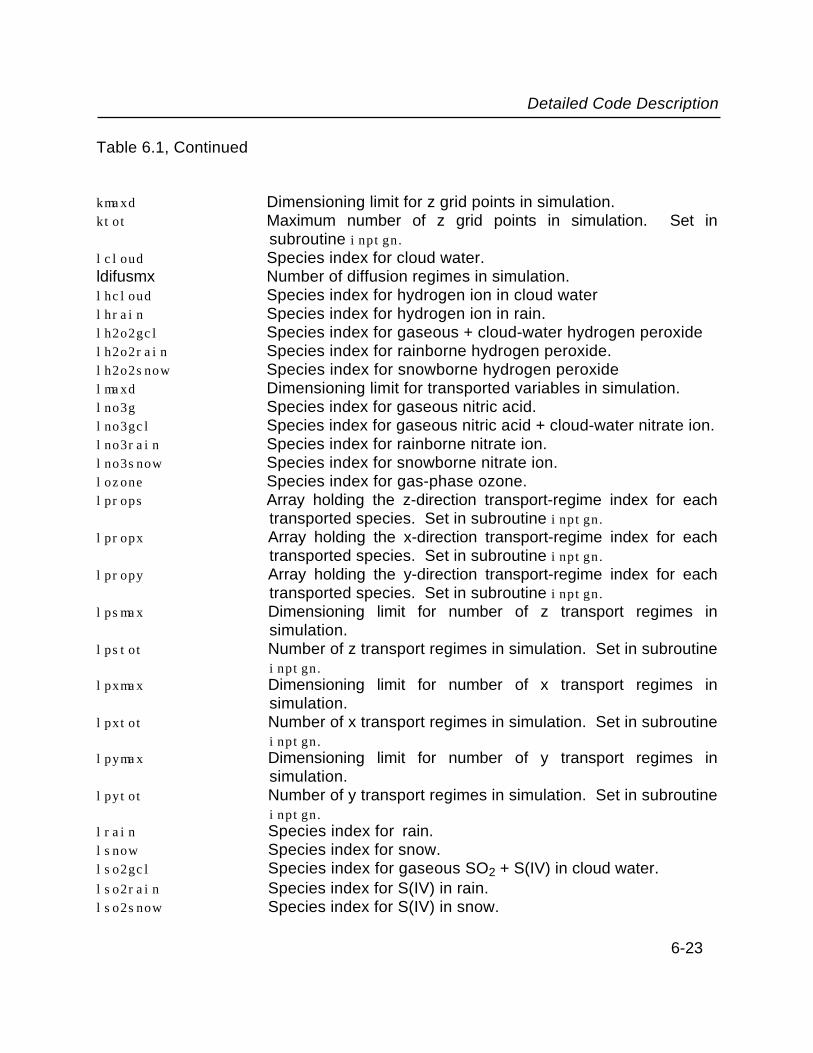
Detailed Code Description
Table 6.1, Continued
kmaxd Dimensioning limit for z grid points in simulation.ktot Maximum number of z grid points in simulation. Set in
subroutine inptgn.lcloud Species index for cloud water.ldifusmx Number of diffusion regimes in simulation.lhcloud Species index for hydrogen ion in cloud waterlhrain Species index for hydrogen ion in rain.lh2o2gcl Species index for gaseous + cloud-water hydrogen peroxidelh2o2rain Species index for rainborne hydrogen peroxide. lh2o2snow Species index for snowborne hydrogen peroxidelmaxd Dimensioning limit for transported variables in simulation.lno3g Species index for gaseous nitric acid.lno3gcl Species index for gaseous nitric acid + cloud-water nitrate ion.lno3rain Species index for rainborne nitrate ion.lno3snow Species index for snowborne nitrate ion.lozone Species index for gas-phase ozone.lprops Array holding the z-direction transport-regime index for each
transported species. Set in subroutine inptgn.lpropx Array holding the x-direction transport-regime index for each
transported species. Set in subroutine inptgn.lpropy Array holding the y-direction transport-regime index for each
transported species. Set in subroutine inptgn.lpsmax Dimensioning limit for number of z transport regimes in
simulation.lpstot Number of z transport regimes in simulation. Set in subroutine
inptgn.lpxmax Dimensioning limit for number of x transport regimes in
simulation.lpxtot Number of x transport regimes in simulation. Set in subroutine
inptgn.lpymax Dimensioning limit for number of y transport regimes in
simulation.lpytot Number of y transport regimes in simulation. Set in subroutine
inptgn.lrain Species index for rain.lsnow Species index for snow.lso2gcl Species index for gaseous SO2 + S(IV) in cloud water.lso2rain Species index for S(IV) in rain.lso2snow Species index for S(IV) in snow.
6-23

Detailed Code Description
Table 6.1, Continued
lso4g Species index for sulfate aerosol.lso4gcl Species index for sulfate aerosol + sulfate ion in cloud water.lso4rain Species index for sulfate ion in rain.lso4snow Species index for sulfate ion in snow.ltemp Index for temperature.ltheta Index for equivalent potential temperature.ltot Number of transported species in simulation. Set in
subroutine inptgn.ltot2 Number of transported plus constrained species in simulation.
Set in subroutine inptgn.lvapcl Species index for water vapor + cloud waterl2maxd Dimensioning limit for transported plus constrained species.
l2maxd = lmaxd + mmaxd.mbndfils Toggle controlling additional filtering at upper and lower inflow
boundaries. If positive, the additional filtering is applied at therespective coordinate boundaries.
mbndfilx Similar to mbndfils, but for x- boundaries.mbndfily Similar to mbndfils, but for y- boundaries.mfreqps Frequency at which transport-property variables are updated
(through subroutine propss) during an z-integration step. Setin subroutine inptgn.legal values are:1 - called once each time in core, during the first zinteg call10, 20 - consider z-integrations as paired within eachsubintegration step (nsubt pairs)10 - called once during first of the pair20 - called once during each of the pair(if nsubt=1, then the 10 and 20 options are like the 1 and 2 options for x and y). Set in subroutine inptgn.
mfreqpx Similar to mfreqps, but pertains to x integrationlegal values are:0 - called only once at start of program - transport propertiesare time invariant1 - called once during the first of the two x-integration in core2 - called once during each of the two x-integrations in coreSet in subroutine inptgn.
mfreqpy Similar to mfreqpx, but pertains to y-integration.
6-24

Detailed Code Description
Table 6.1, Continued
mgen Control variable for chemical/physical transformationintegration; if 1, then the transformation integrations areperformed; if 0, they are skipped. Set in subroutine inptgn.
mmaxd Dimensioning limit for constrained species in simulation.mtemp Energy balance integration control variable: 1 - energy
balance calculated and equivalent potential temperature is atransported variable; 0 - energy balance is not calculated:temperature is a constrained variable. Set in subroutineinptgn.
mtitle Character variable containing title of simulation.mtrans Transport integration control variable; if 1, then z integrations
are performed; if 0, then z integrations are skipped. Set insubroutine inptgn.
mtranx Transport integration control variable; if 1, then x integrationsare performed; if 0, then x integrations are skipped. Set insubroutine inptgn.
mtrany Transport integration control variable; if 1, then y integrationsare performed; if 0, then y integrations are skipped. Set insubroutine inptgn.
munifs Specifies uniform/non-uniform grid in vertical direction: 1 ifuniform; 0 otherwise. Set in subroutine inptgn.
munifx Specifies uniform/non-uniform grid in x-direction: 1 if uniform;0 otherwise. Set in subroutine inptgn.
munify Specifies uniform/non-uniform grid in y-direction: 1 if uniform;0 otherwise. Set in subroutine inptgn.
name Character arrays containing names of species in simulation.ncorr Number of corrector passes applied in ODE integrator. Set in
subroutine inptgn.nfilsrch Parameter in filter subroutine (see subroutine foresfilt listing
in Table 40). Set in subroutine inptgn.nfiltitr Parameter in filter subroutine (see subroutine foresfilt listing
in Table 40). Set in subroutine inptgn.nfilts Number of z-integration steps between filtering. Set in
subroutine inptgn.nfiltset Parameter in filter subroutine (see subroutine foresfilt
listing in Table 40). Set in subroutine inptgn.nfiltx Number of x-integration steps between filtering. Set in
subroutine inptgn.
6-25
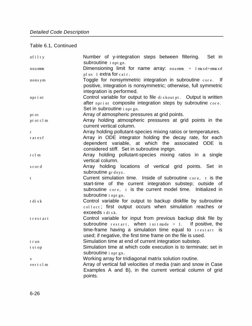
Detailed Code Description
Table 6.1, Continued
nfilty Number of y-integration steps between filtering. Set insubroutine inptgn.
nnammx Dimensioning limit for name array: nnammx = lmaxd+mmaxdplus 1 extra for cair.
nonsym Toggle for nonsymmetric integration in subroutine core. Ifpositive, integration is nonsymmetric; otherwise, full symmetricintegration is performed.
nprint Control variable for output to file diskoutpt. Output is writtenafter nprint composite integration steps by subroutine core.Set in subroutine inptgn.
ptot Array of atmospheric pressures at grid points.ptotclm Array holding atmospheric pressures at grid points in the
current vertical column.r Array holding pollutant-species mixing ratios or temperatures.ratesf Array in ODE integrator holding the decay rate, for each
dependent variable, at which the associated ODE isconsidered stiff. Set in subroutine inptgn.
rclm Array holding pollutant-species mixing ratios in a singlevertical column.
scord Array holding locations of vertical grid points. Set insubroutine grdxyz.
t Current simulation time. Inside of subroutine core, t is thestart-time of the current integration substep; outside ofsubroutine core, t is the current model time. Initialized insubroutine inptgn.
tdisk Control variable for output to backup diskfile by subroutinecollect; first output occurs when simulation reaches orexceeds tdisk.
trestart Control variable for input from previous backup disk file bysubroutine restart, when initmode = 1. If positive, thetime-frame having a simulation time equal to trestart isused; if negative, the first time frame on the file is used.
trun Simulation time at end of current integration substep.tstop Simulation time at which code execution is to terminate; set in
subroutine inptgn.v Working array for tridiagonal matrix solution routine.vertclm Array of vertical fall velocities of media (rain and snow in Case
Examples A and B), in the current vertical column of gridpoints.
6-26

Detailed Code Description
Table 6.1, Continued
winds Array of vertical wind components at grid points. Computed insubroutine wind.
windsclm Array of vertical wind components in the current verticalcolumn of grid points.
windx Array of x wind components at grid points. Computed insubroutine wind.
windy Array of y wind components at grid points. Computed insubroutine wind.
xcord Array holding locations of x grid points. Set in subroutinegrdxyz
ycord Array holding locations of y grid points. Set in subroutinegrdxyz.
Table 6.2: Listing of Main Program pluvius
program pluvius include "pluvius.com"cc Main program for pluvius code: initializes, then cycles throughc progressive time steps and terminates when model time equals tstop.cc Enter control variables, various initialization parameters, andc computation grid.c call inptgncc Set up finite-element parameters.c call femsetcc Set initial values of dependent-variable arrays.c call initcc Input initial wind field.c call windcc Set up output files and write initial dependent-variable arrays.
6-27
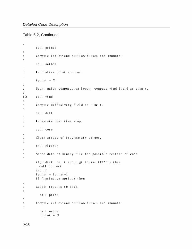
Detailed Code Description
Table 6.2, Continued
c call printicc Compute inflow and outflow fluxes and amounts.c call matbalcc Initialize print counter.c iprint = Occ Start major computation loop: compute wind field at time t.c1O call windcc Compute diffusivity field at time t.c call diffcc Integrate over time step.c call corecc Clean arrays of fragmentary values.c call cleanupcc Store data on binary file for possible restart of code.c if(itdisk .ne. O.and.t.gt.tdisk-.OO1*dt) then
call collect end if iprint = iprint+1 if (iprint.ge.nprint) thencc Output results to disk.c call printcc Compute inflow and outflow fluxes and amounts.c call matbal iprint = O
6-28

Detailed Code Description
Table 6.2, Continued
endifcc The following is a "security blanket" to inform the user that c computation is proceeding. It prints to screen the current time, c plus three parameters at grid point 1,19,15 in the interior of thec computational domain:c 1. the temperaturec 2. the saturation mixing ratio of water vaporc 3. the sum of cloud+vapor water minus the saturation valuec This print block should be removed as soon as the user has c sufficient confidence that the test codes in Examples A and B c are operating properly.c rr=sat(r(1,19,15,ltemp))/cair(1,19,15) dif= r(1,19,15,lvapcl)-rr write(6,21) t,r(1,19,15,ltemp),rr,dif21 format(1h ,'time, temp, sat, diff = ',4(e12.6,1x))c if (t.lt.tstop) go to 1O stop end
Table 6.3a: Listing of Include File pluvius.com for Case Example A
c-------------------------------------------------------------------cc pluvius II include file for Case Example A -- met. onlycc-------------------------------------------------------------------------
parameter( imaxd=1, jmaxd=33, kmaxd=37)parameter( ijkmax = 37)parameter( lmaxd=4, l2maxd=7, mmaxd=3 )parameter( lpxmax=1, lpymax=2, lpsmax=4 )parameter( ldifusmx=lpsmax )parameter( nnammx= l2maxd+mmaxd+2 )
c
6-29

Detailed Code Description
Table 6.3a, Continued
c imaxd, jmaxd, kmaxd, = dimensioning limits for x, y, and z.c ijkmax = maximum of imaxd,jmaxd, and kmaxd.c lmaxd = dimensioning limit for transported species.c l2maxd = dimensioning limit for species contained in r array.c mmaxd = dimensioning for steady-state species.c lpxmax,lpymax,lpsmax= dimensioning limits for consolidated parameters:c normally lpxmax=lpymax=1 and lpsmax may be 3 or 4.c ldifusmx = dimensioning limit for vertical eddy diffusivity.c ldifusmx = 1 when all vertical regimes have same diffusivities.c ldifusmx = lpsmx when regimes have different diffusivities.cc Set key thermodynamic parameters.c
parameter( gamdry =-9.76e-5) !dry adiabatic lapse rate (deg. k/cm)parameter( cp=2.91e8) !air heat capacity (erg/mole deg.k)parameter( glc=8.314e7) !gas-law const. (erg/mole deg. k)parameter( heatc=4.5e11) !lat. heat of cond. (erg/mole)parameter( heats=5.O2e11) !lat. heat of sub. (erg/mole)parameter( heatf=5.2e1O) !lat. heat of fusion (erg/mole)parameter( ak=O.286) !r/cpparameter( alocp=1725.) !heatc/cp (deg. k)
c c Number of grid points, species, transport regimes.c
common /arrays/itot,jtot,ktot,ltot,ltot2,lpstot, + lpytot,lpxtotc c itot, jtot, ktot = number of x, y, and z grid points.c ltot = actual number of transported species.c ltot2 = actual number of species in r array.c lpstot = actual number of phases used to compute vertical transport.c lpytot, lpxtot = ditto for y- and x-directions.cc Species names and output title.c
common /names/ name, mtitlecharacter mtitle*(8O)character*1O name(nnammx)
cc Note: these names are for printout only, and control nothing else c within the code.cc name = 1O character species name
6-30
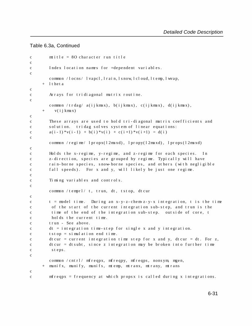
Detailed Code Description
Table 6.3a, Continued
c mtitle = 8O character run title cc Index location names for =dependent variables.c
common /locns/ lvapcl,lrain,lsnow,lcloud,ltemp,lwvap, + lthetacc Arrays for tridiagonal matrix routine.c
common /trdag/ a(ijkmax), b(ijkmax), c(ijkmax), d(ijkmax), + v(ijkmax)cc These arrays are used to hold tri-diagonal matrix coefficients and c solution. tridag solves system of linear equations:c a(i-1)*v(i-1) + b(i)*v(i) + c(i+1)*v(i+1) = d(i)c
common /regime/ lpropx(l2maxd), lpropy(l2maxd), lprops(l2maxd)cc Holds the x-regime, y-regime, and z-regime for each species. In c z-direction, species are grouped by regime. Typically will have c rain-borne species, snow-borne species, and others (with negligible c fall speeds). For x and y, will likely be just one regime.cc Timing variables and controls.c
common /temprl/ t, trun, dt, tstop, dtcurcc t = model time. During an x-y-z-chem-z-y-x integration, t is the timec of the start of the current integration sub-step, and trun is the c time of the end of the integration sub-step. outside of core, t c holds the current time.c trun - See above.c dt = integration time-step for single x and y integration.c tstop = simulation end time.c dtcur = current integration time step for x and y, dtcur = dt. For z, c dtcur = dtsubt, since z integration may be broken into further time c steps.c
common /cntrl/ mfreqpx, mfreqpy, mfreqps, nonsym, mgen, + munifx, munify, munifs, mtemp, mtranx, mtrany, mtranscc mfreqpx = frequency at which propsx is called during x integrations.
6-31

Detailed Code Description
Table 6.3a, Continued
c legal values are:c 1 - called once during the first of the 2 x-integration in core.c 2 - called once during each of the 2 x-integrations in core.c mfreqpy - similar but for propsy.c mfreqpz - similar but for propss.c O - called once at start of program.c 1 - called once each time in core, during the first zinteg call.c 1O, 2O - consider z-integrations as paired within eachc subintegration step (nsubt pairs).c 1O - called once during first of the pair.c 2O - called once during each of the pair.c (if nsubt=1, then the 1O and 2O options are like the 1 and 2c options for x and y.)c nonsym - if positive, a non-symmetric integration is performed - just c x-y-z-chem.c mgen - subroutine chmint is only called if mgen>O.c munifsx, munify, munifs - a positive value means x, y, or s/z gridc spacing is uniform. used in filtering routine to improve efficiency.c mtranx, mtrany, mtrans - if positive, then x,y, or s transport is c computed. if negative or zero, transport is skipped.c mtemp = control variable for energy-balance calculations.c 1 - energy balance calculated: temperature is a dependent variablec O - energy balance is not calculated: temperature is a constrained c variable (if used at all).cc Grid structures and associated computational factors inc finite-element determination.c
common /grid/ + ct1a(3,ijkmax), ct1c(3,ijkmax), ct3b(3,ijkmax), + ct3h(3,ijkmax), ct3a(3,ijkmax), ct3d(3,ijkmax), + ct3f(3,ijkmax), ct3c(3,ijkmax), ct4b(3,ijkmax), + ct4d(3,ijkmax), ct3e(3,ijkmax), ct3df(3,ijkmax), + ct2a, ct2c, + xcord(imaxd), deltax(imaxd), fdcofx(3,imaxd), + ycord(jmaxd), deltay(jmaxd), fdcofy(3,jmaxd), + scord(kmaxd), deltas(kmaxd), fdcofs(3,kmaxd), + xwidth(imaxd),ywidth(jmaxd),swidth(kmaxd)cc xcord(i) = x coordinate at grid point ic ycord(i) = y coordinate at grid point jc scord(i) = s coordinate at grid point kc
6-32
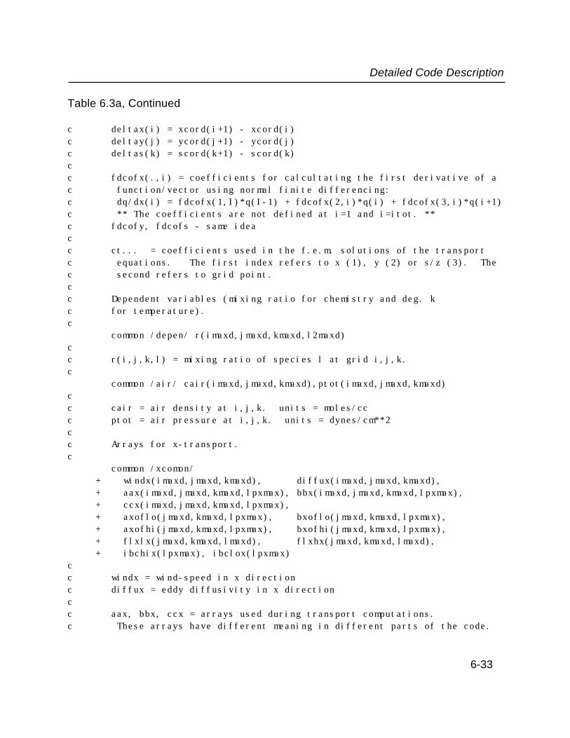
Detailed Code Description
Table 6.3a, Continued
c deltax(i) = xcord(i+1) - xcord(i)c deltay(j) = ycord(j+1) - ycord(j)c deltas(k) = scord(k+1) - scord(k)cc fdcofx(.,i) = coefficients for calcultating the first derivative of a c function/vector using normal finite differencing:c dq/dx(i) = fdcofx(1,I)*q(I-1) + fdcofx(2,i)*q(i) + fdcofx(3,i)*q(i+1)c ** The coefficients are not defined at i=1 and i=itot. **c fdcofy, fdcofs - same ideacc ct... = coefficients used in the f.e.m. solutions of the transport c equations. The first index refers to x (1), y (2) or s/z (3). The c second refers to grid point.cc Dependent variables (mixing ratio for chemistry and deg. k c for temperature).c
common /depen/ r(imaxd,jmaxd,kmaxd,l2maxd) cc r(i,j,k,l) = mixing ratio of species l at grid i,j,k.c
common /air/ cair(imaxd,jmaxd,kmaxd),ptot(imaxd,jmaxd,kmaxd)cc cair = air density at i,j,k. units = moles/ccc ptot = air pressure at i,j,k. units = dynes/cm**2cc Arrays for x-transport.c
common /xcomon/ + windx(imaxd,jmaxd,kmaxd), diffux(imaxd,jmaxd,kmaxd), + aax(imaxd,jmaxd,kmaxd,lpxmax), bbx(imaxd,jmaxd,kmaxd,lpxmax), + ccx(imaxd,jmaxd,kmaxd,lpxmax), + axoflo(jmaxd,kmaxd,lpxmax), bxoflo(jmaxd,kmaxd,lpxmax), + axofhi(jmaxd,kmaxd,lpxmax), bxofhi(jmaxd,kmaxd,lpxmax), + flxlx(jmaxd,kmaxd,lmaxd), flxhx(jmaxd,kmaxd,lmaxd), + ibchix(lpxmax), ibclox(lpxmax)cc windx = wind-speed in x directionc diffux = eddy diffusivity in x directioncc aax, bbx, ccx = arrays used during transport computations.c These arrays have different meaning in different parts of the code.
6-33

Detailed Code Description
Table 6.3a, Continued
c In propsx, we define:c dr/dt = aax * d2r/dx2 + bbx * dr/dx + ccx * rc (Note: for x, ccx is zero. for s/z, ccs is non-zero.)c These values are used by coeffs to define new aax, bbx, ccx withc meaningc aax(i,..)*r(i-1,..) + bbx(i,..)*r(i,..) c + ccx(i,..)*r(i+1,..) + oldint(i,..) = O.cc axoflo,bxoflo-hold values of aax & bbx (as defined in propsx) at i=1.c axofhi,bxofhi-hold values of aax & bbx (as defined in propsx) at c i=itot.c flxlx, flxhs - hold fluxes at i=1 and i=itot boundaries.c ibchix, ibclox - boundary condition specifier. Note that these arec defined for each regime, not each species.c 1 = flux b.c. if inflow or no-flow at a boundary, but outflow b.c. if c there is outflow.c Anything else = "forced outflow" which gives zero flux if there c turns out to be inflow.cc Arrays for y-transport.c
common /ycomon/ + windy(imaxd,jmaxd,kmaxd), diffuy(imaxd,jmaxd,kmaxd), + aay(imaxd,jmaxd,kmaxd,lpymax), bby(imaxd,jmaxd,kmaxd,lpymax), + ccy(imaxd,jmaxd,kmaxd,lpymax), + ayoflo(imaxd,kmaxd,lpymax), byoflo(imaxd,kmaxd,lpymax), + ayofhi(imaxd,kmaxd,lpymax), byofhi(imaxd,kmaxd,lpymax), + flxly(imaxd,kmaxd,lmaxd), flxhy(imaxd,kmaxd,lmaxd), + ibchiy(lpymax), ibcloy(lpymax)cc Arrays for vertical transport.c
common /scomon/ + winds(imaxd,jmaxd,kmaxd),diffus(imaxd,jmaxd,kmaxd,lpsmax), + vertcl(imaxd,jmaxd,kmaxd,lpsmax), + aas(kmaxd,lpsmax), bbs(kmaxd,lpsmax), ccs(kmaxd,lpsmax), + asoflo(lpsmax), bsoflo(lpsmax), csoflo(lpsmax), + asofhi(lpsmax), bsofhi(lpsmax), csofhi(lpsmax), + flxls(imaxd,jmaxd,lmaxd), flxhs(imaxd,jmaxd,lmaxd), + ibchis(lpsmax), ibclos(lpsmax), + jfog(imaxd,jmaxd,kmaxd), dbydz2(ijkmax), + drain(kmaxd), dsnow(kmaxd), vrain(kmaxd), vsnow(kmaxd)c
6-34

Detailed Code Description
Table 6.3a, Continued
c Much of this parallels xcomon. However, since s/z integrations are c performed one column at a time, most of the computational variablesc have no i-j dimensions.cc diffus = vertical eddy diffusivity. Note fourth dimension whichc may be used if one does energy equation and has different diffusivity c for energy and trace substances.c vertcl = settling velocity for each regime. Negative (or zero) exceptc for helium.c jfog=saturation flag- jfog = 1 if air is saturated or supersaturated.c drain, dsnow = pseudo-diffusivity for rain and snow.c vrain, vsnow = vertical fall velocities for rain and snow.
common /column/ rclm(kmaxd,l2maxd), windsclm(kmaxd), + cairclm(kmaxd), difusclm(kmaxd,lpsmax),ptotclm(kmaxd), + vertcclm(kmaxd,lpsmax), flxlsclm(lmaxd), flxhsclm(lmaxd)cc z-chem-z integrations are performed one "column" at a time. During the c integration, variables are moved from their 3 or 4 dimensional arrays c into these smaller "_clm" arrays, then back at the integration end. c this reduces page faulting.c
common / print_com / nprint, dtdisk, tdisk, itdiskcc nprint = subroutine print is called from main program after c nprint calls to corec dtdisk = disk output at increments of dtdiskc tdisk = next disk output at this timec itdisk = O - no disk outputc other - disk output occursc Note - tdisk is updated as output occurs. it can be c initialized to zero (get initial output) or non-zero values.c
common / filter / nfiltx, nfilty, nfilts, + nfilsrch,nfiltset,nfiltitr, + filfacx(lmaxd), filfacy(lmaxd), filfacs(lmaxd), + mbndfilx, mbndfily, mbndfilscc nfiltx = filtering in x direction will occur after this manyc x-integrations.c filfacx(l) = x-direction filter factor for species l. if filteringc is to be done, use O.1O. for no filtering, use O.c (this may be unnecessary. normally one would filter all or no
6-35
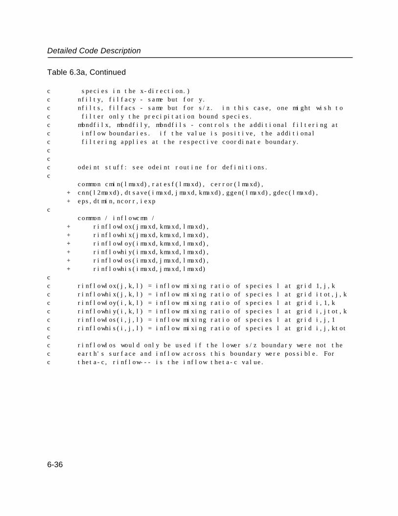
Detailed Code Description
Table 6.3a, Continued
c species in the x-direction.)c nfilty, filfacy - same but for y.c nfilts, filfacs - same but for s/z. in this case, one might wish toc filter only the precipitation bound species.c mbndfilx, mbndfily, mbndfils - controls the additional filtering at c inflow boundaries. if the value is positive, the additional c filtering applies at the respective coordinate boundary.ccc odeint stuff: see odeint routine for definitions.c
common cmin(lmaxd),ratesf(lmaxd), cerror(lmaxd), + cnn(l2maxd),dtsave(imaxd,jmaxd,kmaxd),ggen(lmaxd),gdec(lmaxd), + eps,dtmin,ncorr,iexpc
common / inflowcmn / + rinflowlox(jmaxd,kmaxd,lmaxd), + rinflowhix(jmaxd,kmaxd,lmaxd), + rinflowloy(imaxd,kmaxd,lmaxd), + rinflowhiy(imaxd,kmaxd,lmaxd), + rinflowlos(imaxd,jmaxd,lmaxd), + rinflowhis(imaxd,jmaxd,lmaxd)cc rinflowlox(j,k,l) = inflow mixing ratio of species l at grid 1,j,kc rinflowhix(j,k,l) = inflow mixing ratio of species l at grid itot,j,kc rinflowloy(i,k,l) = inflow mixing ratio of species l at grid i,1,kc rinflowhiy(i,k,l) = inflow mixing ratio of species l at grid i,jtot,kc rinflowlos(i,j,l) = inflow mixing ratio of species l at grid i,j,1c rinflowhis(i,j,l) = inflow mixing ratio of species l at grid i,j,ktotcc rinflowlos would only be used if the lower s/z boundary were not the c earth's surface and inflow across this boundary were possible. For c theta-c, rinflow--- is the inflow theta-c value.
6-36

Detailed Code Description
Table 6.3b: Listing of Include File pluvius.com for Case Example B
c-------------------------------------------------------------------cc pluvius II include file for Case Example B -- chem. onlycc------------------------------------------------------------------------- parameter( imaxd=1, jmaxd=33, kmaxd=37) parameter( ijkmax = 37) parameter( lmaxd=15, l2maxd=22, mmaxd=7 ) parameter( lpxmax=1, lpymax=2, lpsmax=4 ) parameter( ldifusmx=lpsmax ) parameter( nnammx= l2maxd+mmaxd+2 )cc imaxd, jmaxd, kmaxd, = dimensioning limits for x, y, and z.c ijkmax = maximum of imaxd,jmaxd, and kmaxd.c lmaxd = dimensioning limit for transported species.c l2maxd = dimensioning limit for species contained in r array.c mmaxd = dimensioning for steady-state species.c lpxmax,lpymax,lpsmax=dimensioning limits for consolidated parameters:c normally lpxmax=lpymax=1 and lpsmax may be 3 or 4.c ldifusmx = dimensioning limit for vertical eddy diffusivity.c ldifusmx = 1 when all vertical regimes have same diffusivities.c ldifusmx = lpsmx when regimes have different diffusivities.cc Set key thermodynamic parameters.c
parameter( gamdry =-9.76e-5) !dry adiabatic lapse rate (deg. k/cm)parameter( cp=2.91e8) !air heat capacity (erg/mole deg.k)parameter( glc=8.314e7) !gas-law const. (erg/mole deg. k)parameter( heatc=4.5e11) !lat. heat of cond. (erg/mole)parameter( heats=5.O2e11) !lat. heat of sub. (erg/mole)parameter( heatf=5.2e1O) !lat. heat of fusion (erg/mole)parameter( ak=O.286) !r/cpparameter( alocp=1725.) !heatc/cp (deg. k)
c c Number of grid points, species, and transport regimes.c common /arrays/itot,jtot,ktot,ltot,ltot2,lpstot, + lpytot, lpxtotc c itot, jtot, ktot = number of x, y, and z grid pointsc ltot = actual number of transported speciesc ltot2 = actual number of species in r array
6-37

Detailed Code Description
Table 6.3b, Continued
c lpstot = actual number of phases used to compute vertical transportc lpytot, lpxtot = ditto for y- and x-directionscc Species names and output title.c common /names/ name, mtitle character mtitle*(8O) character*1O name(nnammx)cc Note: these names are for printout only, and control nothing else c within the code.cc name = 1O character species namec mtitle = 8O character run titlecc Location names for dependent variables.c common /locns/ lvapcl,lrain,lsnow,lcloud,ltemp,lhrain, + lhcloud,lso2gcl,lso2rain,lso2snow,lso4g,lso4gcl, + lso4rain,lso4snow,lno3g,lno3gcl,lno3rain,lno3snow, + lh2o2gcl,lh2o2rain,lh2o2snow,lozonecc Arrays for tridiagonal matrix routine.c
common /trdag/ a(ijkmax), b(ijkmax), c(ijkmax), d(ijkmax), + v(ijkmax)cc These arrays are used to hold tri-diagonal matrix coefficients and c solution. tridag solves system of linear equations:c a(i-1)*v(i-1) + b(i)*v(i) + c(i+1)*v(i+1) = d(i)c common /regime/ lpropx(l2maxd), lpropy(l2maxd), lprops(l2maxd)cc Holds the x-regime, y-regime, and z-regime for each species. In c z-direction, species are grouped by regime. Typically will have c rain-borne species, snow-borne species, and others (with negligible c fall speeds). For x and y, will likely be just one regime.cc Timing variables and controls.c common /temprl/ t, trun, dt, tstop, dtcurcc t = model time. During an x-y-z-chem-z-y-x integration, t is the time
6-38
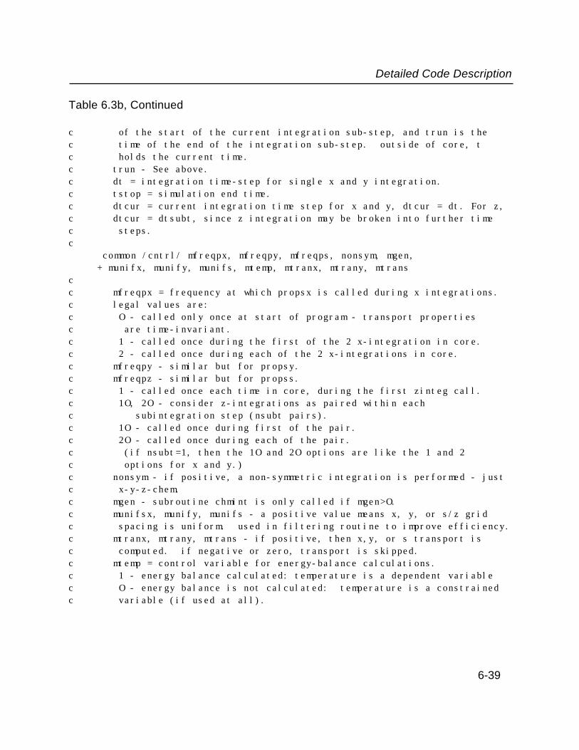
Detailed Code Description
Table 6.3b, Continued
c of the start of the current integration sub-step, and trun is the c time of the end of the integration sub-step. outside of core, t c holds the current time.c trun - See above.c dt = integration time-step for single x and y integration.c tstop = simulation end time.c dtcur = current integration time step for x and y, dtcur = dt. For z, c dtcur = dtsubt, since z integration may be broken into further time c steps.c common /cntrl/ mfreqpx, mfreqpy, mfreqps, nonsym, mgen, + munifx, munify, munifs, mtemp, mtranx, mtrany, mtranscc mfreqpx = frequency at which propsx is called during x integrations.c legal values are:c O - called only once at start of program - transport properties c are time-invariant.c 1 - called once during the first of the 2 x-integration in core.c 2 - called once during each of the 2 x-integrations in core.c mfreqpy - similar but for propsy.c mfreqpz - similar but for propss.c 1 - called once each time in core, during the first zinteg call.c 1O, 2O - consider z-integrations as paired within eachc subintegration step (nsubt pairs).c 1O - called once during first of the pair.c 2O - called once during each of the pair.c (if nsubt=1, then the 1O and 2O options are like the 1 and 2 c options for x and y.)c nonsym - if positive, a non-symmetric integration is performed - just c x-y-z-chem.c mgen - subroutine chmint is only called if mgen>O.c munifsx, munify, munifs - a positive value means x, y, or s/z gridc spacing is uniform. used in filtering routine to improve efficiency.c mtranx, mtrany, mtrans - if positive, then x,y, or s transport is c computed. if negative or zero, transport is skipped.c mtemp = control variable for energy-balance calculations.c 1 - energy balance calculated: temperature is a dependent variablec O - energy balance is not calculated: temperature is a constrained c variable (if used at all).
6-39

Detailed Code Description
Table 6.3b, Continued
c Grid structures and associated computational factors inc finite-element determination.c common /grid/ + ct1a(3,ijkmax), ct1c(3,ijkmax), ct3b(3,ijkmax), + ct3h(3,ijkmax), ct3a(3,ijkmax), ct3d(3,ijkmax), + ct3f(3,ijkmax), ct3c(3,ijkmax), ct4b(3,ijkmax), + ct4d(3,ijkmax), ct3e(3,ijkmax), ct3df(3,ijkmax), + ct2a, ct2c, + xcord(imaxd), deltax(imaxd), fdcofx(3,imaxd), + ycord(jmaxd), deltay(jmaxd), fdcofy(3,jmaxd), + scord(kmaxd), deltas(kmaxd), fdcofs(3,kmaxd), + xwidth(imaxd),ywidth(jmaxd),swidth(kmaxd)cc xcord(i) = x coordinate at grid point ic ycord(i) = y coordinate at grid point jc scord(i) = s coordinate at grid point kcc deltax(i) = xcord(i+1) - xcord(i)c deltay(j) = ycord(j+1) - ycord(j)c deltas(k) = scord(k+1) - scord(k)cc fdcofx(.,i) = coefficients for calcultating the first derivative of a c function/vector using normal finite differencing:c dq/dx(i) = fdcofx(1,i)*q(i-1) + fdcofx(2,i)*q(i) + fdcofx(3,i)*q(i+1)c ** The coefficients are not defined at i=1 and i=itot. **c fdcofy, fdcofs - same ideacc ct... = coefficients used in the f.e.m. solutions of the transport c equations. The first index refers to x (1), y (2) or s/z (3). The c second refers to grid point.cc Dependent variables (mixing ratio for chemistry and deg. k c for temperature).c
common /depen/ r(imaxd,jmaxd,kmaxd,l2maxd) cc r(i,j,k,l) = mixing ratio of species l at grid i,j,k.c
common /air/ cair(imaxd,jmaxd,kmaxd),ptot(imaxd,jmaxd,kmaxd)cc cair = air density at i,j,k. units = moles/cc
6-40

Detailed Code Description
Table 6.3b, Continued
c ptot = air pressure at i,j,k. units = dynes/cm**2cc Arrays for x-transport.c common /xcomon/ + windx(imaxd,jmaxd,kmaxd), diffux(imaxd,jmaxd,kmaxd), + aax(imaxd,jmaxd,kmaxd,lpxmax), bbx(imaxd,jmaxd,kmaxd,lpxmax), + ccx(imaxd,jmaxd,kmaxd,lpxmax), + axoflo(jmaxd,kmaxd,lpxmax), bxoflo(jmaxd,kmaxd,lpxmax), + axofhi(jmaxd,kmaxd,lpxmax), bxofhi(jmaxd,kmaxd,lpxmax), + flxlx(jmaxd,kmaxd,lmaxd), flxhx(jmaxd,kmaxd,lmaxd), + ibchix(lmaxd), ibclox(lmaxd)cc windx = wind-speed in x directionc diffux = eddy diffusivity in x directioncc aax, bbx, ccx=computational arrays used during transport computations.c These arrays have different meaning in different parts of the code. c In propsx, we define:c dr/dt = aax * d2r/dx2 + bbx * dr/dx + ccx * rc (Note: for x, ccx is zero. for s/z, ccs is non-zero.)c These values are used by coeffs to define new aax, bbx, ccx withc meaningc aax(i,..)*r(i-1,..) + bbx(i,..)*r(i,..) c + ccx(i,..)*r(i+1,..) + oldint(i,..) = O.cc axoflo,bxoflo-hold values of aax & bbx (as defined in propsx) at i=1.c axofhi,bxofhi-hold values of aax & bbx(as defined in propsx)at i=itot.c flxlx, flxhs - hold fluxes at i=1 and i=itot boundaries.c ibchix, ibclox - boundary condition specifier. Note that these arec defined for each regime, not each species.c 1 = flux b.c. if inflow or no-flow at a boundary, but outflow b.c. if c there is outflow.c Anything else = "forced outflow" which gives zero flux if there c turns out to be inflow.cc Arrays for y-transport.c common /ycomon/ + windy(imaxd,jmaxd,kmaxd), diffuy(imaxd,jmaxd,kmaxd), + aay(imaxd,jmaxd,kmaxd,lpymax), bby(imaxd,jmaxd,kmaxd,lpymax), + ccy(imaxd,jmaxd,kmaxd,lpymax),
6-41
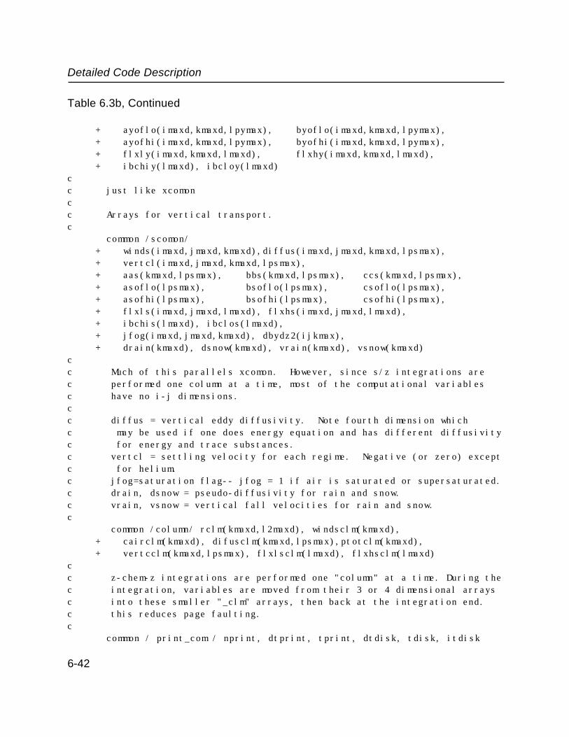
Detailed Code Description
Table 6.3b, Continued
+ ayoflo(imaxd,kmaxd,lpymax), byoflo(imaxd,kmaxd,lpymax), + ayofhi(imaxd,kmaxd,lpymax), byofhi(imaxd,kmaxd,lpymax), + flxly(imaxd,kmaxd,lmaxd), flxhy(imaxd,kmaxd,lmaxd), + ibchiy(lmaxd), ibcloy(lmaxd)cc just like xcomoncc Arrays for vertical transport.c common /scomon/ + winds(imaxd,jmaxd,kmaxd),diffus(imaxd,jmaxd,kmaxd,lpsmax), + vertcl(imaxd,jmaxd,kmaxd,lpsmax), + aas(kmaxd,lpsmax), bbs(kmaxd,lpsmax), ccs(kmaxd,lpsmax), + asoflo(lpsmax), bsoflo(lpsmax), csoflo(lpsmax), + asofhi(lpsmax), bsofhi(lpsmax), csofhi(lpsmax), + flxls(imaxd,jmaxd,lmaxd), flxhs(imaxd,jmaxd,lmaxd), + ibchis(lmaxd), ibclos(lmaxd), + jfog(imaxd,jmaxd,kmaxd), dbydz2(ijkmax), + drain(kmaxd), dsnow(kmaxd), vrain(kmaxd), vsnow(kmaxd)cc Much of this parallels xcomon. However, since s/z integrations are c performed one column at a time, most of the computational variables c have no i-j dimensions.cc diffus = vertical eddy diffusivity. Note fourth dimension whichc may be used if one does energy equation and has different diffusivity c for energy and trace substances.c vertcl = settling velocity for each regime. Negative (or zero) exceptc for helium.c jfog=saturation flag-- jfog = 1 if air is saturated or supersaturated.c drain, dsnow = pseudo-diffusivity for rain and snow.c vrain, vsnow = vertical fall velocities for rain and snow.c
common /column/ rclm(kmaxd,l2maxd), windsclm(kmaxd), + cairclm(kmaxd), difusclm(kmaxd,lpsmax),ptotclm(kmaxd), + vertcclm(kmaxd,lpsmax), flxlsclm(lmaxd), flxhsclm(lmaxd)cc z-chem-z integrations are performed one "column" at a time. During the c integration, variables are moved from their 3 or 4 dimensional arrays c into these smaller "_clm" arrays, then back at the integration end. c this reduces page faulting.c common / print_com / nprint, dtprint, tprint, dtdisk, tdisk, itdisk
6-42

Detailed Code Description
Table 6.3b, Continued
c nprint = subroutine print is called from main program after c nprint calls to corec dtdisk = disk output at increments of dtdiskc tdisk = next disk output at this timec itdisk = O - no disk outputc other - disk output occursc Note - tdisk is updated as output occurs. It can be c initialized to zero (get initial output) or non-zero values.c common / filter / nfiltx, nfilty, nfilts, + nfilsrch,nfiltset,nfiltitr, + filfacx(lmaxd), filfacy(lmaxd), filfacs(lmaxd), + mbndfilx, mbndfily, mbndfilscc nfiltx = filtering in x direction will occur after this manyc x-integrations.c filfacx(l) = x-direction filter factor for species l. if filteringc is to be done, use O.1O. for no filtering, use O.c (this may be unnecessary. normally one would filter all or noc species in the x-direction.)c nfilty, filfacy - same but for y.c nfilts, filfacs - same but for s/z. in this case, one might wish toc filter only the precipitation bound species.c mbndfilx, mbndfily, mbndfils - controls the additional filtering at c inflow boundaries. if the value is positive, the additional c filtering applies at the respective coordinate boundary.ccc odeint stuff: see odeint routine for definitions.c common cmin(lmaxd),ratesf(lmaxd), cerror(lmaxd), + cnn(l2maxd),dtsave(imaxd,jmaxd,kmaxd),ggen(lmaxd),gdec(lmaxd), + eps,dtmin,ncorr,iexpc
common / inflowcmn / + rinflowlox(jmaxd,kmaxd,lmaxd), + rinflowhix(jmaxd,kmaxd,lmaxd), + rinflowloy(imaxd,kmaxd,lmaxd), + rinflowhiy(imaxd,kmaxd,lmaxd), + rinflowlos(imaxd,jmaxd,lmaxd), + rinflowhis(imaxd,jmaxd,lmaxd)
6-43

Detailed Code Description
Table 6.3b, Continued
c rinflowlox(j,k,l) = inflow mixing ratio of species l at grid 1,j,kc rinflowhix(j,k,l) = inflow mixing ratio of species l at grid itot,j,kc rinflowloy(i,k,l) = inflow mixing ratio of species l at grid i,1,kc rinflowhiy(i,k,l) = inflow mixing ratio of species l at grid i,jtot,kc rinflowlos(i,j,l) = inflow mixing ratio of species l at grid i,j,1c rinflowhis(i,j,l) = inflow mixing ratio of species l at grid i,j,ktotcc rinflowlos would only be used if the lower s/z boundary were not the c earth's surface and inflow across this boundary were possible. For c theta-c, rinflow--- is the inflow theta-c value.
Table 6.4a: Listing of Subroutine inptgn for Case Example A
subroutine inptgncc Class I subroutine called from program pluviuscc Version for Case Example Acc Inptgn initializes species names and indices, and grid indices. It also c sets a number of control variables, including subroutine bypass c controls, printing and time limits, and controls for execution of the c odeint ordinary differential-equation integrator.
include 'pluvius.com'cc Set initialization mode initmode. c If initmode = O compute initial conditions.c If initmode = 1 initialize by reading historical data from disk.c Historical data can be modified within this subroutine, if desired.c initmode=O ! Don't read from disk file for initialization.cc Set dimensionality of integration domain.c
mtrans =1
6-44
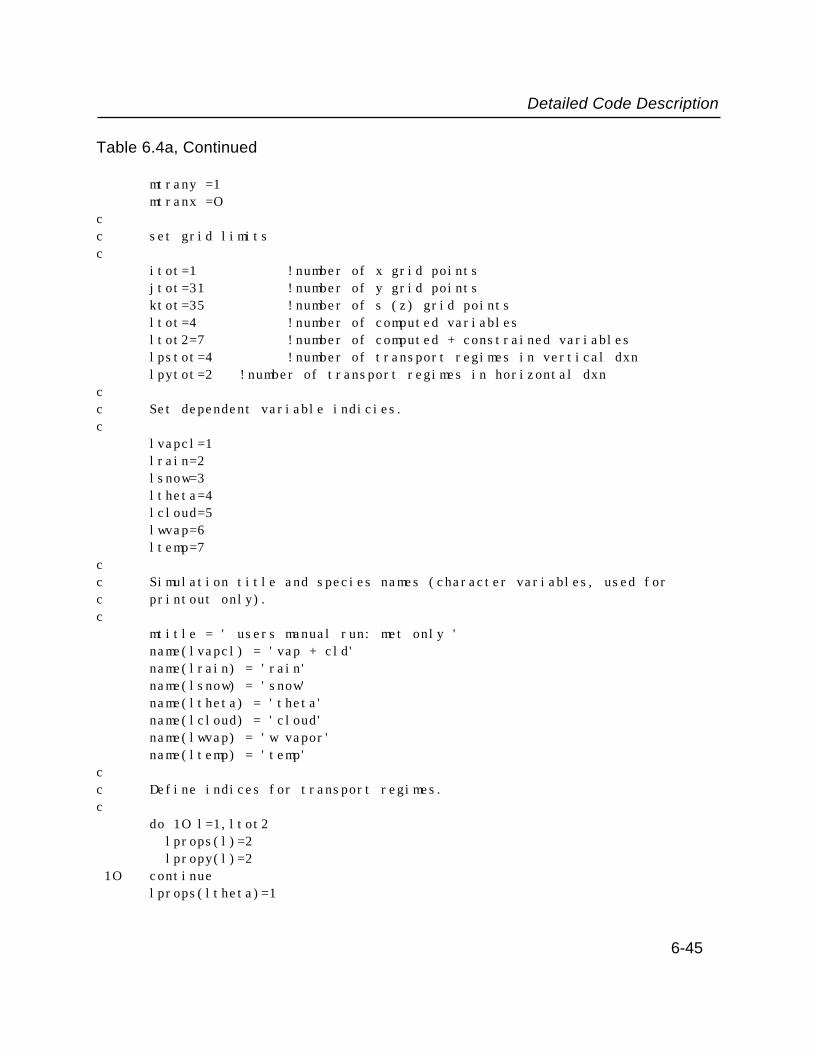
Detailed Code Description
Table 6.4a, Continued
mtrany =1mtranx =O
cc set grid limitsc
itot=1 !number of x grid pointsjtot=31 !number of y grid pointsktot=35 !number of s (z) grid pointsltot=4 !number of computed variablesltot2=7 !number of computed + constrained variableslpstot=4 !number of transport regimes in vertical dxnlpytot=2 !number of transport regimes in horizontal dxn
cc Set dependent variable indicies.c
lvapcl=1lrain=2lsnow=3ltheta=4lcloud=5lwvap=6ltemp=7
cc Simulation title and species names (character variables, used for c printout only).c
mtitle = ' users manual run: met only 'name(lvapcl) = 'vap + cld'name(lrain) = 'rain'name(lsnow) = 'snow'name(ltheta) = 'theta'name(lcloud) = 'cloud'name(lwvap) = 'w vapor'name(ltemp) = 'temp'
cc Define indices for transport regimes.c
do 1O l=1,ltot2 lprops(l)=2 lpropy(l)=2
1O continuelprops(ltheta)=1
6-45

Detailed Code Description
Table 6.4a, Continued
lprops(lvapcl)=2lprops(lrain)=3lprops(lsnow)=4lprops(lcloud)=2lprops(lwvap)=2lprops(ltemp)=2lpropy(ltheta)=1lpropy(lvapcl)=2lpropy(lrain)=2lpropy(lsnow)=2lpropy(lcloud)=2lpropy(lwvap)=2lpropy(ltemp)=2
cc Set disk output controls:cc print control for primary data output file "diskoutpt":c
nprint=48O !write every 72OO sec @ 2*dt=15 seccc print controls for unformatted backup file "dskbackup":c
itdisk=2 ! disk output: 1=continuous; 2=single updated frametdisk= 36OO. !start backup disk at 36OO secdtdisk= 36OO. !redo backup disk at 36OO sec increments
cc Set time spacing and limit.
t=O.dt=7.5tstop= 36OOO.
cc Set spatial domain and grid.cc Set spatial grids.cc dsunif, dxunif, dyunif = grid lengths for uniform grid; IF A GRID IS c NONUNIFORM, SET ITS d_unif VALUE TO ZERO. Also if a grid is nonuniform, c set its array _cord here. Otherwise the array(s) will be set in call c to subroutine grdxyz.c
dxunif = O.dsunif = 15OOO.dyunif = 1375OOO.
6-46

Detailed Code Description
Table 6.4a, Continued
scord(1) = O.ycord(1) = O.
cc grdxyz sets the grid positions xcord, ycord, and scord for the case ofc a uniform grid.c
call grdxyz(dxunif,dyunif,dsunif)cc Set o.d.e. integrator (odeint) parameters (see odeint for definitions).c
eps=O.O1dtmin=1.e-1Oncorr=1iexp=1do 3O l=1,lmaxd ratesf(l)=1.e-2 cmin(l)=1.e-24
3O continuecmin(ltheta) = 1.e-8cmin(lvapcl) = 1.e-17cmin(lrain) = 1.e-17cmin(lsnow) = 1.e-17do 4O k = 1, ltot cerror(k) = cmin(k)*1.e4
4O continuec Set boundary conditions: 1 = flux b.c. if inflow or no-flow at a c boundary, but outflow b.c. if there is outflow.c Anything else = "forced outflow" which gives zero-gradient under inflow c conditions.c do 5O l=1,ltot ibchis(l)=1 ibclos(l)=1 ibchiy(l)=1 ibcloy(l)=1 5O continuecc Set subroutine calling frequencies.c
mfreqpy=2 !called on all occasionsmfreqps=2O !called on all occasionsmgen = 1 !call gen during all occasions
6-47

Detailed Code Description
Table 6.4a, Continued
mtemp=1 !energy balance integratednonsym=-1 !symmetric integration performed
cc Set filter controls.c
nfilts = 1 !filter calls at each integration stepnfilty = 1nfilsrch = 4nfiltset = 2nfiltitr = 3
cc Turn on filters for all species.c do 6O l=1,ltot filfacs(l)=O.1 filfacy(l)=O.1 6O continuec c boundary filtersc
mbndfilx=-1mbndfily=1mbndfils=1returnend
Table 6.4b: Listing of Subroutine inptgn for Case Example B
subroutine inptgncc Class I subroutine called from program pluviuscc Version for Case Example Bcc Inptgn initializes species names and indices, and grid indices. It c also sets a number of control variables, including subroutine bypass c controls, printing and time limits, and controls for execution of the c odeint ordinary differential-equation integrator.c
6-48

Detailed Code Description
Table 6.4b, Continued
include 'pluvius.com'cc Set initialization mode initmode. c If initmode = O compute initial conditions.c If initmode = 1 initialize by reading historical data from disk.c Historical data can be modified within this subroutine, if desired.c
initmode=O ! Don't read from disk file for initialization.ccc Set dimensionality of integration domain.c
mtrans =1mtrany =1mtranx =O
cc set grid limitsc
itot=1 !number of x grid pointsjtot=31 !number of y grid pointsktot=35 !number of s (z) grid pointsltot= 15 !number of computed variablesltot2= 22 !number of computed + constrained variableslpstot=4 !number of transport regimes in vertical dxnlpytot=2 !number of transport regimes in y-dxn
cc Set dependent variable indices.c lso2gcl = 1 lso2rain = 2 lso2snow = 3 lso4g = 4 lso4gcl = 5 lso4rain =6 lso4snow =7 lno3gcl =8 lno3g =9 lno3rain =1O lno3snow =11 lh2o2gcl =12 lh2o2rain =13
lh2o2snow =14
6-49

Detailed Code Description
Table 6.4b, Continued
lozone =15 lcloud = 16 lrain = 17 lsnow = 18 ltemp = 19 lhcloud = 2O lhrain = 21 lvapcl = 22cc Simulation title and species names (character variables, used for c printout only).c mtitle = ' user manual run: chemistry simulation ' name(lso2gcl) = 'g+c so2' name(lso2rain) = 'rain so2' name(lso2snow) = 'snow so2' name(lso4g) = 'g so4' name(lso4gcl) = 'g+c so4' name(lso4rain) = 'rain so4' name(lso4snow) = 'snow so4' name(lno3gcl) = 'g+c no3' name(lno3g) = 'g no3' name(lno3rain) = 'rain no3' name(lno3snow) = 'snow no3' name(lh2o2gcl) = 'g+c h2o2' name(lh2o2rain) = 'rain h2o2' name(lh2o2snow) = 'snow h2o2' name(lozone) = 'ozone' name(ltot+1) = 'cloud' name(ltot+2) = 'rain' name(ltot+3) = 'snow' name(ltot+4) = 'temp' name(ltot+5) = 'cloud h+' name(ltot+6) = 'rain h+' name(ltot+7) = 'c+w vap'cc Define indices for transport regimes: regime indices arbitrarily chosen c here to be consistent with Case Example A, which solved energy equationc and used index 1 for theta.c do 2O l=1,ltot2 lpropy(l)=2
lprops(l)=2
6-50

Detailed Code Description
Table 6.4b, Continued
2O continue lprops(lso2gcl)=2 lprops(lso2rain)=3 lprops(lso2snow)=4 lprops(lso4g)=2 lprops(lso4gcl)=2 lprops(lso4rain)=3 lprops(lso4snow)=4 lprops(lno3g)=2 lprops(lno3gcl)=2 lprops(lno3rain)=3 lprops(lno3snow)=4 lprops(lh2o2gcl)=2 lprops(lh2o2rain)=3 lprops(lh2o2snow)=4 lprops(lozone)=2 lprops(lsnow)=4 lprops(lrain)=3cc Set disk output controls:cc print control for primary data output file "dskoutpt":c
nprint=48O !write every 72OO sec @ 2*dt=15 seccc print controls for unformatted backup file "dskbackup"c
itdisk=2 ! disk output: 1=continuous; 2=single updated frame tdisk= 36OO. !start backup disk at 36OO sec
dtdisk= 36OO. !redo backup disk at 36OO sec incrementscc Set time spacing and limit.c
t=O.dt=7.5tstop= 36OOO.
cc Set spatial domain and grid.cc Set spatial grids.cc dsunif, dxunif, dyunif = grid lengths for uniform grid; IF A GRID IS
6-51

Detailed Code Description
Table 6.4b, Continued
c NONUNIFORM, SET ITS d_unif VALUE TO ZERO. Also if a grid is nonuniform, c set its array _cord here. Otherwise the array(s) will be set in call c to subroutine grdxyz.c
dxunif = O.dsunif = 15OOO.dyunif = 1375OOO.scord(1) = O.ycord(1) = O.
cc grdxyz sets the grid positions xcord, ycord, and scord for the case ofc a uniform grid.c call grdxyz(dxunif,dyunif,dsunif)cc Set o.d.e. integrator (odeint) parameters (see odeint for definitions).c eps=O.O1 dtmin=1.e-1O ncorr=1 iexp=1 do 3O l=1,ltot ratesf(l)=1.e-2 cmin(l)=1.e-243O continue do 4O l = l, ltot cerror(l) = cmin(l)*1.e44O continuecc Set boundary conditions: 1 = flux b.c. if inflow or no-flow at a c boundary, but outflow b.c. if there is outflow.c Anything else = "forced outflow" which gives zero-gradient under inflow c conditions.c do 5O l=1,ltot ibchis(l)=1 ibclos(l)=1 ibchiy(l)=1 ibcloy(l)=15O continuecc Set subroutine calling frequencies.c
6-52

Detailed Code Description
Table 6.4b, Continued
mfreqpy=2 !called on all occasions mfreqps=2O !called on all occasions mgen = 1 !call gen during all occasions mijpack=1 !pack/unpack mtemp=O !energy balance not integrated nonsym=-1 !symmetric integration performedcc Set filter controls.c nfilts = 1 !filter calls at each integration step nfilty = 1 nfilsrch = 4 nfiltset = 2 nfiltitr = 3cc Turn on filters for all species.c do 6O l=1,ltot filfacs(l)=O.1 filfacy(l)=O.1 6O continue cc boundary filtersc mbndfilx=-1 mbndfily=1 mbndfils=1 return end
6-53

Detailed Code Description
Table 6.5: Listing of Subroutine femset
subroutine femset include 'pluvius.com'cc Class II subroutine called from program pluviuscc femset computes grid expansion factors and common grid terms for c subsequent use in numerical approximations. Interrogated only oncec during program execution.c do 1O i = 1,ijkmax do 1O idum = 1,3 ct1a(idum,i) = O. ct1c(idum,i) = O. ct3a(idum,i) = O. ct3b(idum,i) = O. ct3c(idum,i) = O. ct3d(idum,i) = O. ct3d(idum,i) = O. ct3e(idum,i) = O. ct3f(idum,i) = O. ct4b(idum,i) = O. ct4d(idum,i) = O. 1O continuecc x coordinatec if (itot.gt.1) then do 2O i = 1,itot-1 deltax(i) = xcord(i+1) - xcord(i) 2O continue do 3O i = 2,itot ct1a(1,i) = 1./deltax(i-1) ct3a(1,i) = deltax(i-1)/12. ct3b(1,i) = deltax(i-1)/6. ct3c(1,i) = deltax(i-1)/4. ct3d(1,i) = deltax(i-1)/3. ct4b(1,i) = deltax(i-1)/2.3O continue do 4O i = 1,itot-1 ct1c(1,i) = 1./deltax(i) ct3e(1,i) = deltax(i)/12. ct3f(1,i) = deltax(i)/3. ct3h(1,i) = deltax(i)/6.
6-54
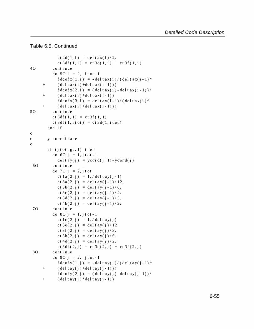
Detailed Code Description
Table 6.5, Continued
ct4d(1,i) = deltax(i)/2. ct3df(1,i) = ct3d(1,i) + ct3f(1,i)4O continue do 5O i = 2, itot-1 fdcofx(1,i) = -deltax(i)/(deltax(i-1)* + (deltax(i)+deltax(i-1))) fdcofx(2,i) = (deltax(i)-deltax(i-1))/ + (deltax(i)*deltax(i-1)) fdcofx(3,i) = deltax(i-1)/(deltax(i)* + (deltax(i)+deltax(i-1)))5O continue ct3df(1,1) = ct3f(1,1) ct3df(1,itot) = ct3d(1,itot) end ifcc y coordinatec if (jtot.gt.1) then do 6O j = 1,jtot-1 deltay(j) = ycord(j+1)-ycord(j) 6O continue do 7O j = 2,jtot ct1a(2,j) = 1./deltay(j-1) ct3a(2,j) = deltay(j-1)/12. ct3b(2,j) = deltay(j-1)/6. ct3c(2,j) = deltay(j-1)/4. ct3d(2,j) = deltay(j-1)/3. ct4b(2,j) = deltay(j-1)/2. 7O continue do 8O j = 1,jtot-1 ct1c(2,j) = 1./deltay(j) ct3e(2,j) = deltay(j)/12. ct3f(2,j) = deltay(j)/3. ct3h(2,j) = deltay(j)/6. ct4d(2,j) = deltay(j)/2. ct3df(2,j) = ct3d(2,j) + ct3f(2,j) 8O continue do 9O j = 2, jtot-1 fdcofy(1,j) = -deltay(j)/(deltay(j-1)* + (deltay(j)+deltay(j-1))) fdcofy(2,j) = (deltay(j)-deltay(j-1))/ + (deltay(j)*deltay(j-1))
6-55
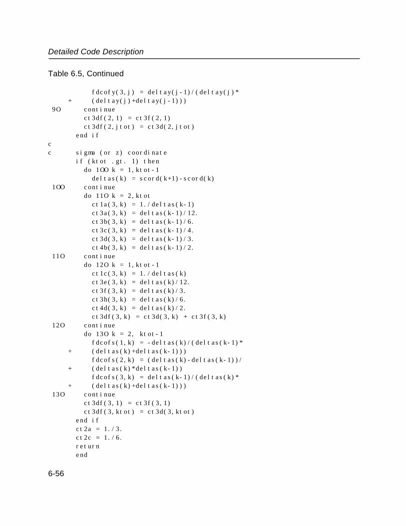
Detailed Code Description
Table 6.5, Continued
fdcofy(3,j) = deltay(j-1)/(deltay(j)* + (deltay(j)+deltay(j-1))) 9O continue ct3df(2,1) = ct3f(2,1) ct3df(2,jtot) = ct3d(2,jtot) end ifcc sigma (or z) coordinate if (ktot .gt. 1) then do 1OO k = 1,ktot-1 deltas(k) = scord(k+1)-scord(k) 1OO continue do 11O k = 2,ktot ct1a(3,k) = 1./deltas(k-1) ct3a(3,k) = deltas(k-1)/12. ct3b(3,k) = deltas(k-1)/6. ct3c(3,k) = deltas(k-1)/4. ct3d(3,k) = deltas(k-1)/3. ct4b(3,k) = deltas(k-1)/2. 11O continue do 12O k = 1,ktot-1 ct1c(3,k) = 1./deltas(k) ct3e(3,k) = deltas(k)/12. ct3f(3,k) = deltas(k)/3. ct3h(3,k) = deltas(k)/6. ct4d(3,k) = deltas(k)/2. ct3df(3,k) = ct3d(3,k) + ct3f(3,k) 12O continue do 13O k = 2, ktot-1 fdcofs(1,k) = -deltas(k)/(deltas(k-1)* + (deltas(k)+deltas(k-1))) fdcofs(2,k) = (deltas(k)-deltas(k-1))/ + (deltas(k)*deltas(k-1)) fdcofs(3,k) = deltas(k-1)/(deltas(k)* + (deltas(k)+deltas(k-1))) 13O continue ct3df(3,1) = ct3f(3,1) ct3df(3,ktot) = ct3d(3,ktot) end if ct2a = 1./3. ct2c = 1./6. return end
6-56

Detailed Code Description
Table 6.6a: Listing of Subroutine init for Case Example A
subroutine initcc Class I subroutine called from program pluviusccc init computes initial values r(i,j,k,l) of the dependent variables for the
entire solution matrix.cc This version of init depicts an idealized warm front.c
include 'pluvius.com'dimension surft(imaxd,jmaxd),surfp(imaxd,jmaxd)data alpha /3.526e-4/ !deg k/cm
cc The following block synthesizes the values based on stipulated surface c conditions and assumed concentration profiles. This will be c unnecessary if real data are available.cc First set surface pressures, temperatures, concentrations, and mixing c ratios.cc Case for preset of met-only computations: set i.c.'s to left of front.c
surft(1,1)=29O. ! deg ksurfp(1,1)=1.O13e6 ! dyne / cm2 unitsjfog(1,1,1)=O
cc cloud flag: jfog = O for clear air, =1 for condensationc
r(1,1,1,ltemp)=surft(1,1)cair(1,1,1)=aircon(surfp(1,1),surft(1,1)) !moles air/ccr(1,1,1,lvapcl)=.65*sat(surft(1,1))/cair(1,1,1)ptot(1,1,1)=surfp(1,1)rr=sat(r(1,1,1,ltemp))/cair(1,1,1)
cc mixing ratio of water in saturated airc
r(1,1,1,lcloud)=dim(r(1,1,1,lvapcl),rr)r(1,1,1,lwvap)=r(1,1,1,lvapcl)-r(1,1,1,lcloud)jfog(1,1,1)=.9999999+r(1,1,1,lcloud)
cc Now estimate air concentrations from approximate integrated
6-57

Detailed Code Description
Table 6.6a, Continued
c hydrostatic equation (j=1 column only).c
do 2O k=2,ktot cair(1,1,k)=cair(1,1,1)*exp(-1.66e-6*scord(k))
cc Now compute temperature profiles based on wet or dry standard lapses.c
r(1,1,k,ltemp)=r(1,1,k-1,ltemp)+rlapse(r(1,1,k-1,ltemp), + cair(1,1,k-1),jfog(1,1,k-1))*deltas(k-1)cc Set humidities and local condensed water flag.
do 1O m=1,3 r(1,1,k,lvapcl)=.65*sat(r(1,1,k,ltemp))/cair(1,1,k) floatk = float(-k+2O) if(k.gt.2O) r(1,1,k,lvapcl) = r(1,1,k,lvapcl)*exp(floatk)
cc (Set 65% rh up to k=2O and decreasing aloft.)c
rr=sat(r(1,1,k,ltemp))/cair(1,1,k) r(1,1,k,lcloud)=dim(r(1,1,k,lvapcl),rr) r(1,1,k,lwvap)=r(1,1,k,lvapcl)-r(1,1,k,lcloud) jfog(1,1,k)=.9999999+r(1,1,k,lcloud) cair(1,1,k)=cair(1,1,k-1)*
+ exp((-alpha-rlapse(r(1,1,k-1,ltemp), + cair(1,1,k-1),jfog(1,1,k)))*deltas(k-1)/ + (O.5*(r(1,1,k-1,ltemp)+r(1,1,k,ltemp)))) 1O continue
ptot(1,1,k)=cair(1,1,k)*glc*r(1,1,k,ltemp) 2O continuecc Now paint j=1 column into interior grid points to right: initialization c array only.c
do 3O j=2,jtot do 3O k=1,ktot do 25 l=1,ltot2 r(1,j,k,l)=O.
25 continue jfog(1,j,k)=O ptot(1,j,k) = ptot(1,1,k) cair(1,j,k)=cair(1,1,k) r(1,j,k,lcloud)=r(1,1,k,lcloud) r(1,j,k,lwvap)=r(1,1,k,lwvap)
6-58
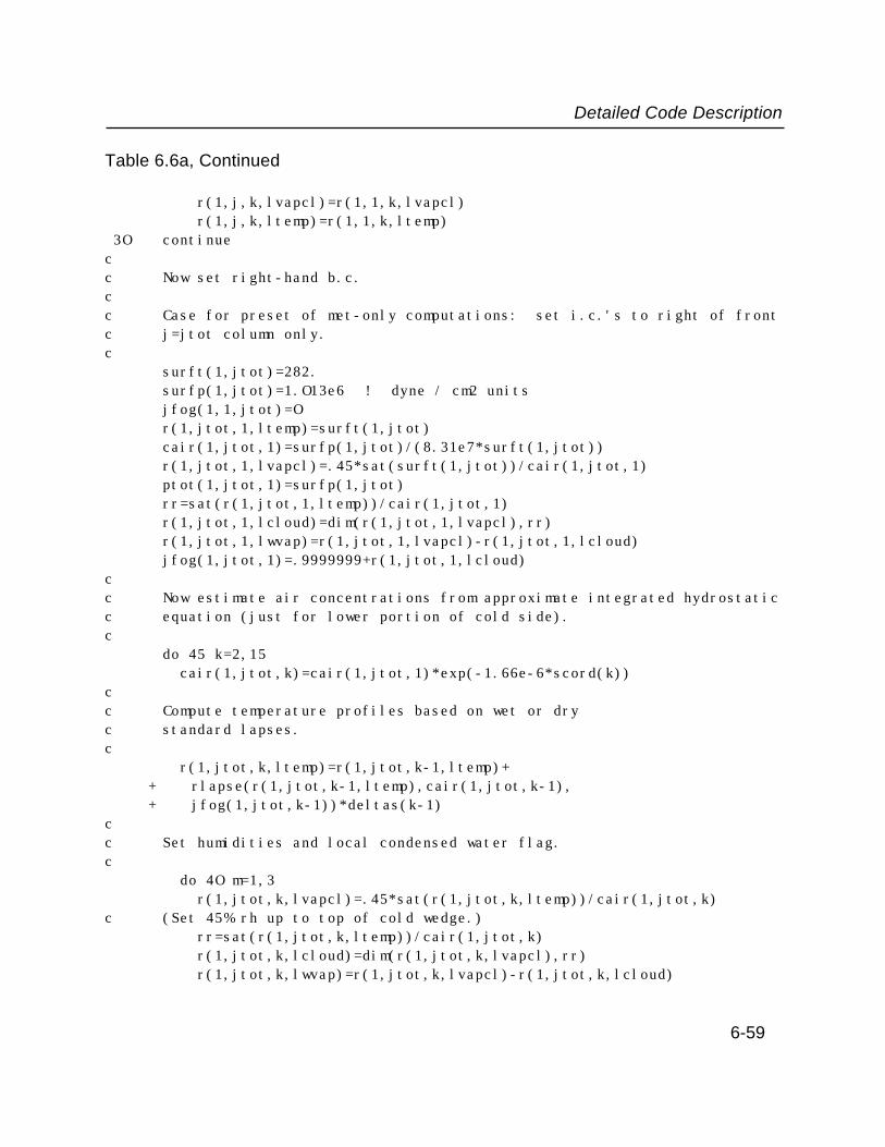
Detailed Code Description
Table 6.6a, Continued
r(1,j,k,lvapcl)=r(1,1,k,lvapcl) r(1,j,k,ltemp)=r(1,1,k,ltemp)
3O continuecc Now set right-hand b.c.cc Case for preset of met-only computations: set i.c.'s to right of frontc j=jtot column only.c
surft(1,jtot)=282.surfp(1,jtot)=1.O13e6 ! dyne / cm2 unitsjfog(1,1,jtot)=Or(1,jtot,1,ltemp)=surft(1,jtot)cair(1,jtot,1)=surfp(1,jtot)/(8.31e7*surft(1,jtot))r(1,jtot,1,lvapcl)=.45*sat(surft(1,jtot))/cair(1,jtot,1)ptot(1,jtot,1)=surfp(1,jtot)rr=sat(r(1,jtot,1,ltemp))/cair(1,jtot,1)r(1,jtot,1,lcloud)=dim(r(1,jtot,1,lvapcl),rr)r(1,jtot,1,lwvap)=r(1,jtot,1,lvapcl)-r(1,jtot,1,lcloud)jfog(1,jtot,1)=.9999999+r(1,jtot,1,lcloud)
cc Now estimate air concentrations from approximate integrated hydrostaticc equation (just for lower portion of cold side).c
do 45 k=2,15 cair(1,jtot,k)=cair(1,jtot,1)*exp(-1.66e-6*scord(k))
cc Compute temperature profiles based on wet or dryc standard lapses.c
r(1,jtot,k,ltemp)=r(1,jtot,k-1,ltemp)+ + rlapse(r(1,jtot,k-1,ltemp),cair(1,jtot,k-1), + jfog(1,jtot,k-1))*deltas(k-1)cc Set humidities and local condensed water flag.c
do 4O m=1,3 r(1,jtot,k,lvapcl)=.45*sat(r(1,jtot,k,ltemp))/cair(1,jtot,k)
c (Set 45% rh up to top of cold wedge.) rr=sat(r(1,jtot,k,ltemp))/cair(1,jtot,k) r(1,jtot,k,lcloud)=dim(r(1,jtot,k,lvapcl),rr) r(1,jtot,k,lwvap)=r(1,jtot,k,lvapcl)-r(1,jtot,k,lcloud)
6-59

Detailed Code Description
Table 6.6a, Continued
jfog(1,jtot,k)=.9999999+r(1,jtot,k,lcloud) cair(1,jtot,k)=cair(1,jtot,k-1)*
+ exp((-alpha-rlapse(r(1,jtot,k-1,ltemp), + cair(1,jtot,k-1),jfog(1,jtot,k)))*deltas(k-1)/ + (O.5*(r(1,jtot,k-1,ltemp)+r(1,jtot,k,ltemp)))) 4O continue
ptot(1,jtot,k)=cair(1,jtot,k)*glc*r(1,jtot,k,ltemp) 45 continuecc Now set initial conditions to right of and below front.c
do 5O j= 7,jtot-1 do 5O k=1,15 jj=j-7 if(k.gt.jj) go to 5O r(1,j,k,ltemp)=r(1,jtot,k,ltemp) r(1,j,k,lvapcl)=r(1,jtot,k,lvapcl) r(1,j,k,lcloud)=r(1,jtot,k,lcloud) r(1,j,k,lwvap)=r(1,j,k,lwvap)
5O continuecc Now compute final pressures, concentrations, and thetas across complete c domain. Note that ptot does not change from this point on.c
do 6O j=1,jtot r(1,j,1,ltheta)=(1.e6/ptot(1,1,1))**ak*r(1,j,1,ltemp)*
+ (1.-alocp*r(1,j,1,lcloud)/r(1,j,1,ltemp)) ptot(1,j,1)=ptot(1,1,1) cair(1,j,1)=ptot(1,j,1)/(glc*r(1,j,1,ltemp)) do 6O k=2,ktot ptot(1,j,k)=ptot(1,j,k-1)*(1.-deltas(k-1)*alpha/r(1,j,k-1,ltemp)) r(1,j,k,ltheta)=(1.e6/ptot(1,j,k))**ak*r(1,j,k,ltemp)*
+ (1.-alocp*r(1,j,k,lcloud)/r(1,j,k,ltemp)) cair(1,j,k)=ptot(1,j,k)/(glc*r(1,j,k,ltemp))
6O continuecc Activate disk read if required.c if(initmode.eq.1) call restart(trestart)ccc Finally, set the (time-invariant) inflow concentrations; these will be c used in the boundary-condition subroutines to determine inflow rates.
6-60

Detailed Code Description
Table 6.6a, Continued
c This should be modified if boundary conditions vary with time.c
call inflowinitreturnend
Table 6.6b: Listing of Subroutine init for Case Example B
subroutine initcc Class I subroutine called from program pluviusc include 'pluvius.com'cc Computes initial values r(i,j,k,l) of the dependent variables for the c entire solution matrix. For this application, the meteorologicalc variables will be supplied through the call of subroutine cloudinit, c which appears immediately below; thus the remainder of subroutine init c will simply compute some of the ancillary variables, plus the chemical c variables, and return.cc Read meteorological input from disk storage.c
call cloudinitcc Set cloud flags.c do 1O j=1,jtot do 1O k=1,ktot jfog(1,j,k)=O if(r(1,j,k,lcloud).gt.O.) jfog(1,j,k)=1cc Compute pressures using equation of state.c ptot(1,j,k)=cair(1,j,k)*glc*r(1,j,k,ltemp) 1O continuec
6-61

Detailed Code Description
Table 6.6b, Continued
c Input initial pollutant mixing ratios.cc Zero internal concentrations.c do 2O j=1,jtot do 2O k=1,ktot do 2O l=1,15 r(1,j,k,l)=O. 2O continuecc Now set mixing ratios throughout.c do 3O k=1,ktot do 3O j=1,jtot if(scord(k).lt.15OOOO) then !below 15OO m layer r(1,j,k,lso2gcl) = 1.e-8 r(1,j,k,lso4g) = 1.e-9 r(1,j,k,lso4gcl) = 1.e-9 r(1,j,k,lno3gcl) = 1.e-9 r(1,j,k,lno3g) = .2e-9 r(1,j,k,lh2o2gcl) = 1.e-9 r(1,j,k,lozone) = 5.e-8 else !above 15OO m layer rr=exp(.OOOO1*(15OOOO.-scord(k))) r(1,j,k,lso2gcl) = 1.e-8*rr r(1,j,k,lso4g) = 1.e-9*rr r(1,j,k,lso4gcl) = 1.e-9*rr r(1,j,k,lno3gcl) = 1.e-9*rr r(1,j,k,lno3g) = .2e-9*rr r(1,j,k,lh2o2gcl) = 1.e-9 r(1,j,k,lozone) = 5.e-8 end if 3O continuecc Activate disk read if required.c if(initmode.eq.1) call restart(trestart)ccc Finally, set the (time-invariant) inflow concentrations; these will be c used in the boundary-condition subroutines to determine inflow rates.c This should be modified if boundary conditions vary with time.
6-62
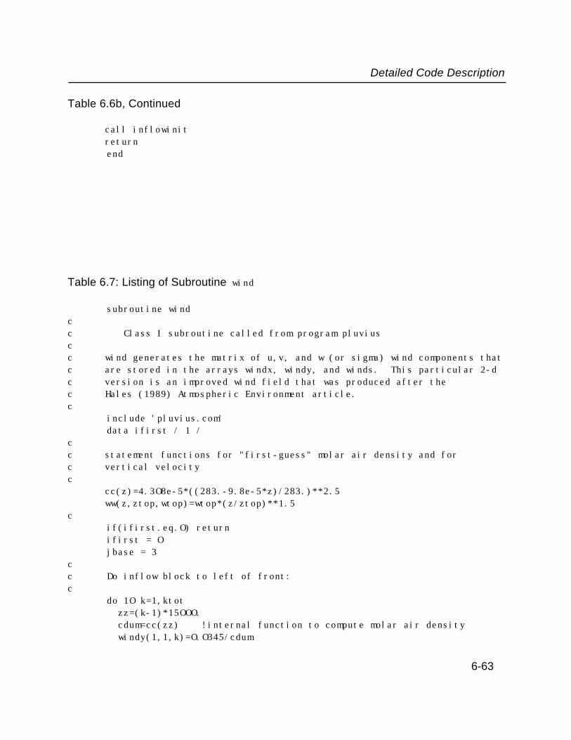
Detailed Code Description
Table 6.6b, Continued
call inflowinitreturn
end
Table 6.7: Listing of Subroutine wind
subroutine windcc Class I subroutine called from program pluviuscc wind generates the matrix of u,v, and w (or sigma) wind components thatc are stored in the arrays windx, windy, and winds. This particular 2-d c version is an improved wind field that was produced after the c Hales (1989) Atmospheric Environment article.c include 'pluvius.com' data ifirst / 1 /cc statement functions for "first-guess" molar air density and forc vertical velocityc
cc(z)=4.3O8e-5*((283.-9.8e-5*z)/283.)**2.5ww(z,ztop,wtop)=wtop*(z/ztop)**1.5
c if(ifirst.eq.O) return ifirst = O jbase = 3cc Do inflow block to left of front:c do 1O k=1,ktot zz=(k-1)*15OOO. cdum=cc(zz) !internal function to compute molar air density windy(1,1,k)=O.O345/cdum
6-63

Detailed Code Description
Table 6.7, Continued
winds(1,1,k)=O. do 1O j=2,jbase-1 windy(1,j,k)=windy(1,1,k) winds(1,j,k)=winds(1,1,k) 1O continuecc do block above frontal slope:c do 2O j=jbase,jbase+12 jj=j-jbase+2 !jj = k index of element just above frontal surface height=(jj-2)*15OOO. slope =.O1O9 if(j.eq.jbase) slope=slope/2 do 2O k=jj,ktot zz=(k-1)*15OOO. airc=cc(zz) zzero=51OOOO.*zz/(51OOOO.-height) airczero=cc(zzero) windyzero=.O345/airczero windy(1,j,k)=windyzero*airczero*51OOOO./ + (airc*(51OOOO.-height)) winds(1,j,k)=windy(1,j,k)*slope*(51OOOO.-zz)/ + (51OOOO.-height) 2O continuecc Fill in winds just on frontal surface (ident. to those just above).c do 3O j=jbase,jbase+13 jj=j-jbase+1 windy(1,j,jj)=windy(1,j,jj+1) winds(1,j,jj)=winds(1,j,jj+1) 3O continue winds(1,jbase,1)=O.cc Now go for inner wedge.c do 4O k=1,12 do 4O j=jbase+k,jbase+13 ktop=j-jbase+1 ! ktop = k index on frontal line ztop=(ktop-1)*15OOO. if(k.ne.1) then zzminus=(k-2)*15OOO. zzplus=k*15OOO.
6-64
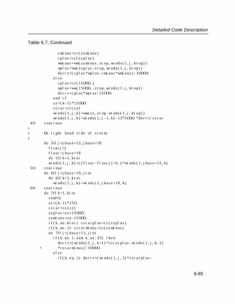
Detailed Code Description
Table 6.7, Continued
cminus=cc(zzminus) cplus=cc(zzplus) wminus=ww(zzminus,ztop,winds(1,j,ktop)) wplus=ww(zzplus,ztop,winds(1,j,ktop)) deriv=(cplus*wplus-cminus*wminus)/3OOOO. else cplus=cc(15OOO.) wplus=ww(15OOO.,ztop,winds(1,j,ktop)) deriv=cplus*wplus/15OOO. end if zz=(k-1)*15OOO. cstar=cc(zz) winds(1,j,k)=ww(zz,ztop,winds(1,j,ktop)) windy(1,j,k)=windy(1,j-1,k)-1375OOO.*deriv/cstar 4O continuecc Do right hand side of storm.c do 5O j=jbase+13,jbase+18 floatj=j float=jbase+18 do 5O k=1,ktot winds(1,j,k)=((float-floatj)/6.)*winds(1,jbase+12,k) 5O continue do 6O j=jbase+19,jtot do 6O k=1,ktot winds(1,j,k)=winds(1,jbase+18,k) 6O continue do 7O k=1,ktot sum=O. zz=(k-1)*15O. cstar=cc(zz) zzplus=zz+15OOO. zzminus=zz-15OOO. if(k.ne.ktot) cstarplus=cc(zzplus) if(k.ne.1) cstarminus=cc(zzminus) do 7O j=jbase+13,jtot if(k.ne.1.and.k.ne.35) then deriv=(winds(1,j,k+1)*cstarplus-winds(1,j,k-1) + *cstarminus)/3OOOO. else if(k.eq.1) deriv=(winds(1,j,2)*cstarplus-
6-65
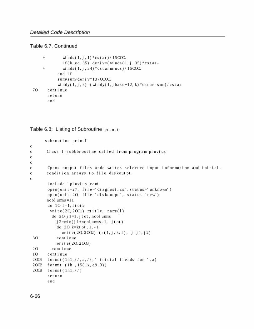
Detailed Code Description
Table 6.7, Continued
+ winds(1,j,1)*cstar)/15OOO. if(k.eq.35) deriv=(winds(1,j,35)*cstar- + winds(1,j,34)*cstarminus)/15OOO. end if sum=sum+deriv*137OOOO. windy(1,j,k)=(windy(1,jbase+12,k)*cstar-sum)/cstar 7O continue return end
Table 6.8: Listing of Subroutine printi
subroutine printicc Class I subbbroutine called from program pluviusccc Opens output files ande writes selected input information and initial-c condition arrays to file diskoutpt.c include 'pluvius.com' open(unit=27, file='diagnostics',status='unknown') open(unit=2O, file='diskoutpt', status='new')
ncolumns=11 do 1O l=1,ltot2 write(2O,2OO1) mtitle, name(l)
do 2O j1=1,jtot,ncolumns j2=min(j1+ncolumns-1, jtot) do 3O k=ktot,1,-1 write(2O,2OO2) (r(1,j,k,l), j=j1,j2)
3O continue write(2O,2OO3)
2O continue 1O continue 2OO1 format(1h1,//,a,//,' initial fields for ',a) 2OO2 format (1h ,15(1x,e9.3)) 2OO3 format(1h1,//) return end
6-66

Detailed Code Description
Table 6.9: Listing of Subroutine print
subroutine printcc Class I subroutine called from program pluviuscc Handles routine printout of computed results to disk.c include 'pluvius.com'
ncolumns=11 do 1Ol=1,ltot2 write(2O,2OO1) mtitle, name(l), t write(2O,2OO4)
do 2O j1=1,jtot,ncolumns j2=min(j1+ncolumns-1, jtot) do 3O k=ktot,1,-1 write(2O,2OO2) (r(1,j,k,l), j=j1,j2)
3O continue write(2O,2OO3)
2O continue 1O continue 2OO1 format(1h1,//,a,//,' fields for ',a,' at time = ',e1O.4,//) 2OO2 format (1h ,15(1x,e9.3)) 2OO3 format(1h1,//,'-4444') !finder tag for subsequent data processing 2OO4 format(1h ,'-9999') !finder tag for subsequent data processing return end
Table 6.10: Listing of Subroutine matbal
subroutine matbalcc Class III subroutine called from program pluvius.cc Subroutine to compute advective inflow/outflow rates at boundaries. c Present version assumes two-dimensional system, and computes rates
6-67

Detailed Code Description
Table 6.10, Continued
c flowing in horizontal(y) direction at left and right, plus rates at c surface. This must be modified for 3-d systems.c Note that, because dry deposition is not computed in this example,c and also because the zero-gradient approximation is made at the y c boundaries, diffusive comnponents of the fluxes are not calculated c here. This should be modified if dry deposition or surface emissionsc are included in downstream applications.c include 'pluvius.com' dimension fsl(ijkmax,l2maxd),flux(ijkmax),total(l2maxd)cc Set print boundaries.c
ncolumns=11cc do lhsc do 5 l=1,ltot2 do 4 k=1,ktot fsl(k,l) = windy(1,1,k)*r(1,1,k,l)*cair(1,1,k) flux(k)=fsl(k,l) 4 continuecc Integrate fluxes across k domain of lhs.c call integrate(flux,scord,ktot,rturn) total(l)=rturn 5 continuecc output lhs values:c do 1O l=1,ltot2
write(2O,*) write(2O,*) "species = ", name(l)
write(2O,*) "LHS horizontal fluxes (moles/cm2-sec or deg./cm2-sec), + for k=1 ... ktot"
do 2O k1=1,ktot,ncolumns k2=min(k1+ncolumns-1, ktot) write(2O,2OO2) (fsl(k,l), k=k1,k2)
2O continue 1O continue write (2O,2OO3) do 5O l=1,ltot2
6-68

Detailed Code Description
Table 6.10, Continued
write(2O,2OO4) l, total(l) 5O continuecc do rhsc do 65 l=1,ltot2 do 6O k=1,ktot fsl(k,l) = windy(1,jtot,k)*r(1,jtot,k,l)*cair(1,jtot,k) flux(k)=fsl(k,l) 6O continuecc Integrate fluxes across k domain on rhs>c call integrate(flux,scord,ktot,rturn) total(l)=rturn 65 continuecc Output rhs statistics:c
do 7O l=1,ltot2 write(2O,*)
write(2O,*) "species = ", name(l) write(2O,*) "RHS horizontal fluxes (moles/cm2-sec or deg/cm2-sec),
+ for k=1 ... ktot" do 8O k1=1,ktot,ncolumns k2=min(k1+ncolumns-1, ktot) write(2O,2OO2) (fsl(k,l), k=k1,k2)
8O continue 7O continue write (2O,2OO7) do 1OO l=1,ltot2 write(2O,2OO4) l, total(l) 1OO continuecc Do bottom. do 11O j=1,jtotcc Compute rain and snow fall velocities at surface.c
call ijpack(1,j) call transport(1,j) do 11O l=1,ltot2
6-69

Detailed Code Description
Table 6.10, Continued
fsl(j,l)=O. if(l.le.ltot) then if(lprops(l).eq.lprops(lrain)) then fsl(j,l)=vertcclm(1,lprops(lrain))*r(1,j,1,l)*cair(1,j,1) end if end if 11O continue do 112 l=1,ltot2 do 111 j=1,jtot flux(j)=fsl(j,l) 111 continuecc Integrate across j domain on grid bottom.c call integrate(flux,ycord,jtot,rturn) total(l)=rturn 112 continuecc Output bottom statistics:c do 12O l=1,ltot2
write(2O,*) write(2O,*) "species = ", name(l)
write(2O,*) "bottom fluxes (moles/cm2-sec), + for j=1 ... jtot"
do 13O j1=1,jtot,ncolumns j2=min(j1+ncolumns-1, jtot) write(2O,2OO2) (fsl(j,l), j=j1,j2)
13O continue 12O continue write (2O,2O11) do 15O l=1,ltot2 write(2O,2OO4) l, total(l) 15O continue 2OO2 format(1h ,/,11(1x,e1O.3)) 2OO3 format (1h ,/,'LHS amounts (moles/cm sec or deg/cm-sec)',//, + ' l amount',/) 2OO4 format(1h ,i3,1x,e1O.4) 2OO6 format(1h ,/,i5,1O(1x,e1O.3)) 2OO7 format (1h ,/,'RHS amounts (moles/cm sec or deg/cm-sec)',//, + ' l amount',/)
6-70
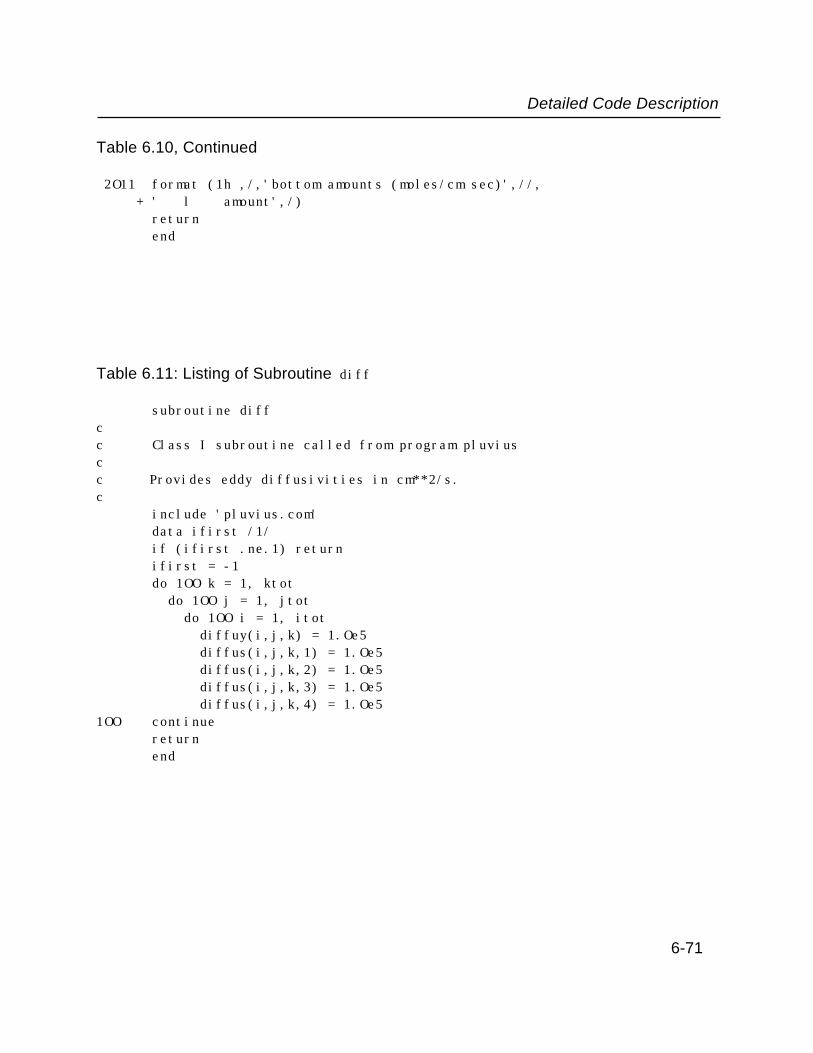
Detailed Code Description
Table 6.10, Continued
2O11 format (1h ,/,'bottom amounts (moles/cm sec)',//, + ' l amount',/) return end
Table 6.11: Listing of Subroutine diff
subroutine diffcc Class I subroutine called from program pluviuscc Provides eddy diffusivities in cm**2/s. c include 'pluvius.com' data ifirst /1/ if (ifirst .ne.1) return ifirst = -1 do 1OO k = 1, ktot do 1OO j = 1, jtot do 1OO i = 1, itot diffuy(i,j,k) = 1.Oe5 diffus(i,j,k,1) = 1.Oe5 diffus(i,j,k,2) = 1.Oe5 diffus(i,j,k,3) = 1.Oe5 diffus(i,j,k,4) = 1.Oe51OO continue return end
6-71

Detailed Code Description
Table 6.12: Listing of Subroutine core
subroutine corecc Class II subroutine called from program pluviuscc Coordinates numerical integration of governing equations for a single c or double time increment, dt ot 2*dt. The choice between a single or c double step is controlled by the variable nonsym (>O for single step; c = O for double step), which is set in subroutine inputgn, a double c step (symmetrical integration) is recommended. This integration processc proceeds as follows: integration in x for dt; integration in y for dt;c integration in s for dt; integration of transformation terms for 2*dt;c integration in s for dt; integration in y for dt; integration in xc for dt.c include 'pluvius.com' data ifirst/1/ dtcur = dt if (ifirst .eq. 1) call coreOO ifirst = Occ Stage 1: initial integration in x (over time dt).c if ((itot.gt.1) .and. (mtranx.gt.O)) then trun = t+dt call xinteg( 1 ) endifcc Stage 2: initial integration in y (over time dt).c if ((jtot.gt.1) .and. (mtrany.gt.O)) then trun = t+dt call yinteg( 1 ) end ifcc Stage 3: (possible) subincrementation of dt into an integral numberc of steps having length dtsub. Initial integration in sigma directionc over period dtsub, composite integration of kinetics step over periodc 2*dtsub, and second integration in sigma direction over next dtsubc increment. Repeat until major time step dt is attained.c tOsave = t do 5O j = 1, jtot
6-72
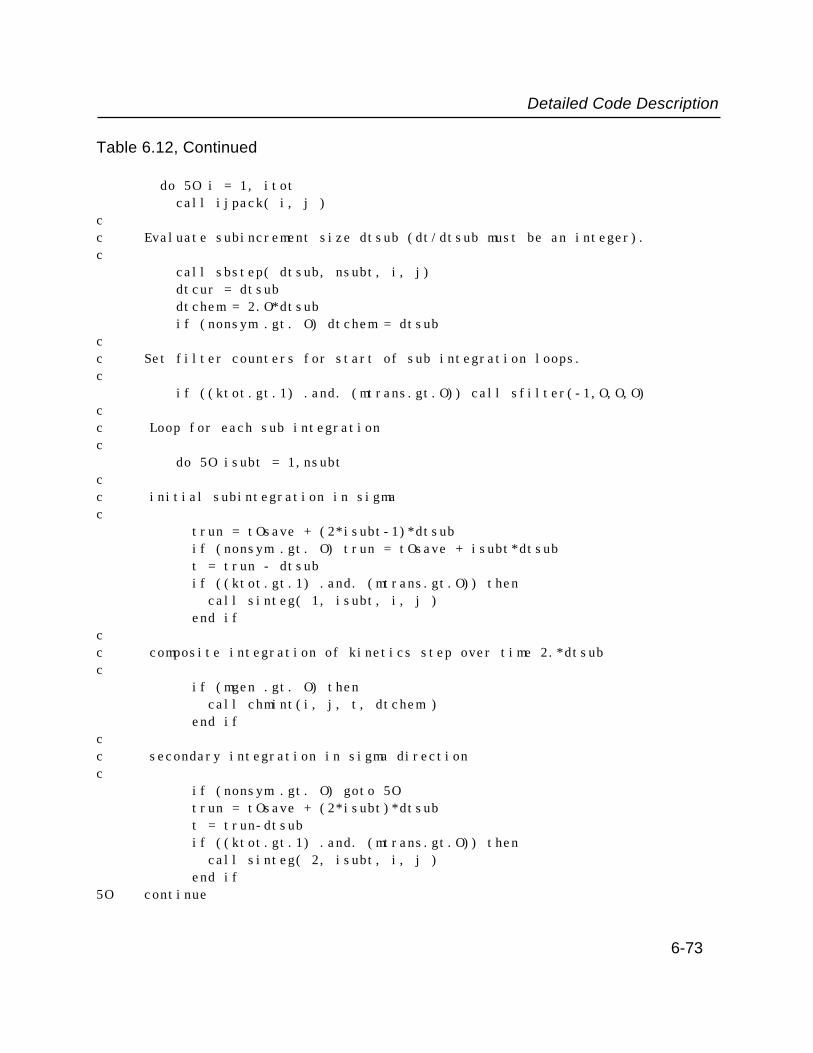
Detailed Code Description
Table 6.12, Continued
do 5O i = 1, itot call ijpack( i, j )cc Evaluate subincrement size dtsub (dt/dtsub must be an integer).c call sbstep( dtsub, nsubt, i, j) dtcur = dtsub dtchem = 2.O*dtsub if (nonsym .gt. O) dtchem = dtsubcc Set filter counters for start of sub integration loops.c if ((ktot.gt.1) .and. (mtrans.gt.O)) call sfilter(-1,O,O,O)cc Loop for each sub integrationc do 5O isubt = 1,nsubtcc initial subintegration in sigmac trun = tOsave + (2*isubt-1)*dtsub if (nonsym .gt. O) trun = tOsave + isubt*dtsub t = trun - dtsub if ((ktot.gt.1) .and. (mtrans.gt.O)) then call sinteg( 1, isubt, i, j ) end ifcc composite integration of kinetics step over time 2.*dtsubc if (mgen .gt. O) then call chmint(i, j, t, dtchem ) end ifcc secondary integration in sigma directionc if (nonsym .gt. O) goto 5O trun = tOsave + (2*isubt)*dtsub t = trun-dtsub if ((ktot.gt.1) .and. (mtrans.gt.O)) then call sinteg( 2, isubt, i, j ) end if5O continue
6-73

Detailed Code Description
Table 6.12, Continued
if ((ktot.gt.1) .and. (mtrans.gt.O)) call sfilter( -2, O, O, O )call ijunpack
cc end stage 3c t = tOsave + dt dtcur = dt if (nonsym .gt. O) goto 9Occ Stage 4: secondary integration in y over time step dt.c if ((jtot.gt.1) .and. (mtrany.gt.O)) then trun = t+dt call yinteg( 2 ) end ifcc Stage 5: secondary integration in x over time step dt.c if ((itot.gt.1) .and. (mtranx.gt.O)) then trun = t+dt call xinteg( 2 ) end if t = t+dt9O continue return end
Table 6.13a: Listing of Subroutine cleanup for Case Example A
subroutine cleanupinclude 'pluvius.com'
cc Class I subroutine called from program pluviuscc User-supplied subroutine to remove extraneous phases and associated c pollutants, as well as to reestablish values of constrained variables
6-74

Detailed Code Description
Table 6.13a, Continued
c after each time step.cc This version is for the met-only demo run for the user's manualc (Case Example A).c
if(mtemp.eq.1) then do 2O j=1,jtot do 2O k=1,ktot
c Calculate temperatures from theta-c's. call tfrmth(ptot(1,j,k),r(1,j,k,ltheta),
+ r(1,j,k,lvapcl),jfog(1,j,k),r(1,j,k,ltemp)) r(1,j,k,lcloud)=r(1,j,k,lvapcl)-
+ sat(r(1,j,k,ltemp))/cair(1,j,k) if(r(1,j,k,lcloud).le.O.) jfog(1,j,k)=O r(1,j,k,lcloud)=amax1(r(1,j,k,lcloud),O.) r(1,j,k,lwvap)=r(1,j,k,lvapcl)-r(1,j,k,lcloud)
2O continueend ifdo 1O j=1,jtot do 1O k=1,ktot !Eliminate any negative mixing ratios. r(1,j,k,lrain)=amax1(r(1,j,k,lrain),O.) r(1,j,k,lsnow)=amax1(r(1,j,k,lsnow),O.) if(r(1,j,k,ltemp).gt.273.2.and.r(1,j,k,lsnow).lt.1.e-5)
+ then !Melt residual snow if above freezing. r(1,j,k,lrain)=r(1,j,k,lrain)+r(1,j,k,lsnow) r(1,j,k,lsnow)=O. end if if(r(1,j,k,lcloud).le.O..and.r(1,j,k,lsnow).lt.1.e-6)
+ then !Sublime residual snow if air subsaturated. r(1,j,k,lvapcl)=r(1,j,k,lvapcl)+r(1,j,k,lsnow) r(1,j,k,lsnow)=O. r(1,j,k,lwvap)=r(1,j,k,lvapcl) end if if(r(1,j,k,lcloud).le.O..and.r(1,j,k,lrain).lt.1.e-5)
+ then !Evaporate residual rain if air subsaturated. r(1,j,k,lvapcl)=r(1,j,k,lvapcl)+r(1,j,k,lrain) r(1,j,k,lrain)=O. r(1,j,k,lwvap)=r(1,j,k,lvapcl)end if
1O continuereturnend
6-75
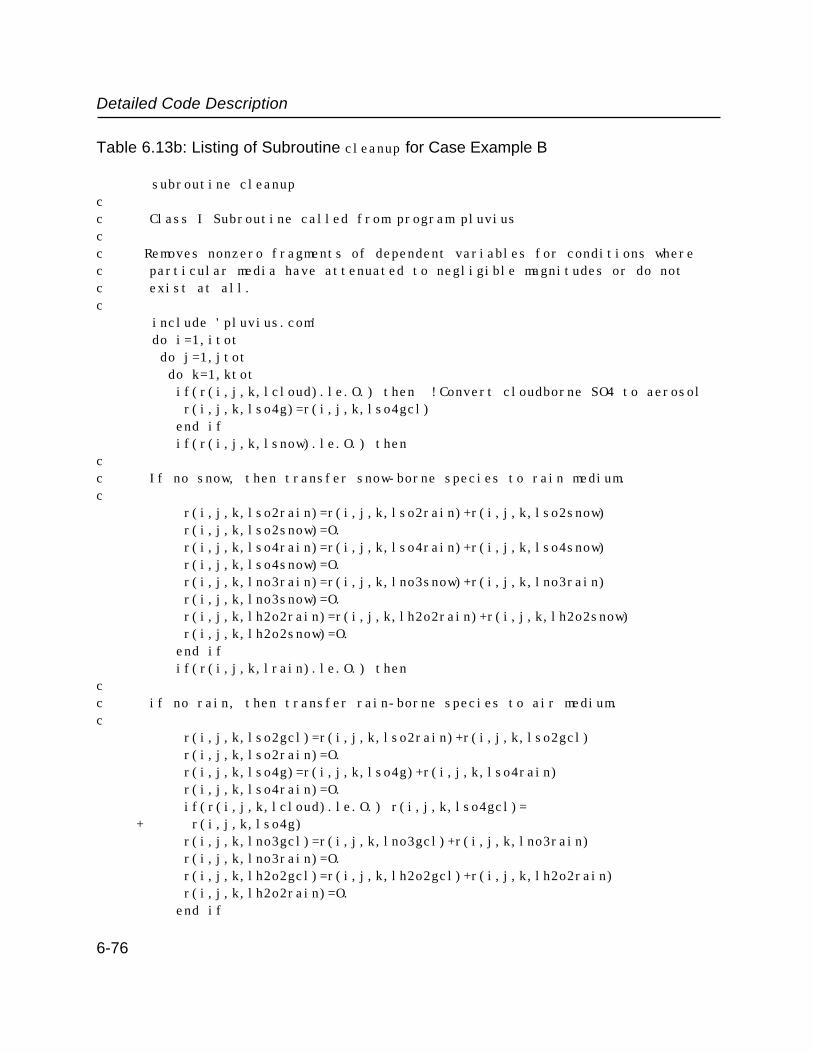
Detailed Code Description
Table 6.13b: Listing of Subroutine cleanup for Case Example B
subroutine cleanupcc Class I Subroutine called from program pluviuscc Removes nonzero fragments of dependent variables for conditions where c particular media have attenuated to negligible magnitudes or do not c exist at all.c include 'pluvius.com' do i=1,itot do j=1,jtot do k=1,ktot if(r(i,j,k,lcloud).le.O.) then !Convert cloudborne SO4 to aerosol r(i,j,k,lso4g)=r(i,j,k,lso4gcl) end if if(r(i,j,k,lsnow).le.O.) thenc c If no snow, then transfer snow-borne species to rain medium.c r(i,j,k,lso2rain)=r(i,j,k,lso2rain)+r(i,j,k,lso2snow) r(i,j,k,lso2snow)=O. r(i,j,k,lso4rain)=r(i,j,k,lso4rain)+r(i,j,k,lso4snow) r(i,j,k,lso4snow)=O. r(i,j,k,lno3rain)=r(i,j,k,lno3snow)+r(i,j,k,lno3rain) r(i,j,k,lno3snow)=O. r(i,j,k,lh2o2rain)=r(i,j,k,lh2o2rain)+r(i,j,k,lh2o2snow) r(i,j,k,lh2o2snow)=O. end if if(r(i,j,k,lrain).le.O.) thencc if no rain, then transfer rain-borne species to air medium.c r(i,j,k,lso2gcl)=r(i,j,k,lso2rain)+r(i,j,k,lso2gcl) r(i,j,k,lso2rain)=O. r(i,j,k,lso4g)=r(i,j,k,lso4g)+r(i,j,k,lso4rain) r(i,j,k,lso4rain)=O. if(r(i,j,k,lcloud).le.O.) r(i,j,k,lso4gcl)= + r(i,j,k,lso4g) r(i,j,k,lno3gcl)=r(i,j,k,lno3gcl)+r(i,j,k,lno3rain) r(i,j,k,lno3rain)=O. r(i,j,k,lh2o2gcl)=r(i,j,k,lh2o2gcl)+r(i,j,k,lh2o2rain) r(i,j,k,lh2o2rain)=O. end if
6-76

Detailed Code Description
Table 6.13b, Continued
end do end do end do return end
Table 6.14: Listing of Subroutine collect
subroutine collectcc Class II subroutine called from program pluviusc include 'pluvius.com' data iend /-7/cc Routine does output to disk file for post-processing.c Parameters are output at time intervals = dtdisk.c if (itdisk .eq. O) returncc Initial entry - write "heading" info. to file.c if (iend .eq. -7) then open( unit=21, file='diskbkup', status='unknown', + form='unformatted') rewind 21 iend = O tdisk = tdisk - .O1*dt ntotp1 = ltot2 + 1 name(ntotp1) = 'cair' write(21) mtitle write(21) itot, jtot, ktot, ntotp1 write(21) (name(k), k=1,ntotp1) write(21) deltax(1), deltay(1), deltas(1) end if write(21) t,
6-77

Detailed Code Description
Table 6.14, Continued
+ ((((r(i,j,k,l), i=1,itot), j=1,jtot), k=1,ktot), + l=1,ltot2), + (((cair(i,j,k), i=1,itot), j=1,jtot), k=1,ktot) write(2O,3OO1) t tdisk=tdisk+dtdiskcc When itdisk=2, save only one time frame. By setting iend=-7, c subsequent entry will overwrite the previous data. if (itdisk.eq.2) then close(21) iend=-7 end if 3OO1 format(1h ,'writing to disk occurred at t = ',e1O.3) return end
Table 6.15: Listing of Subroutine restart
subroutine restartcc Class II subroutine called from subroutine inputgncc Initializes the dependent variables by reading their values from the c backup file written by a previous run. That backup file must c be renamed from "diskbkup" to "rstinpt". Logical unit 21 is used c for reading the file.cc trestart - the record (or time slice) on the backup file having this c time is used.c
include 'pluvius.com'
character*8O mtitlerstcharacter*1O namerst(nnammx)
cc Open "rstinpt" file.c
6-78
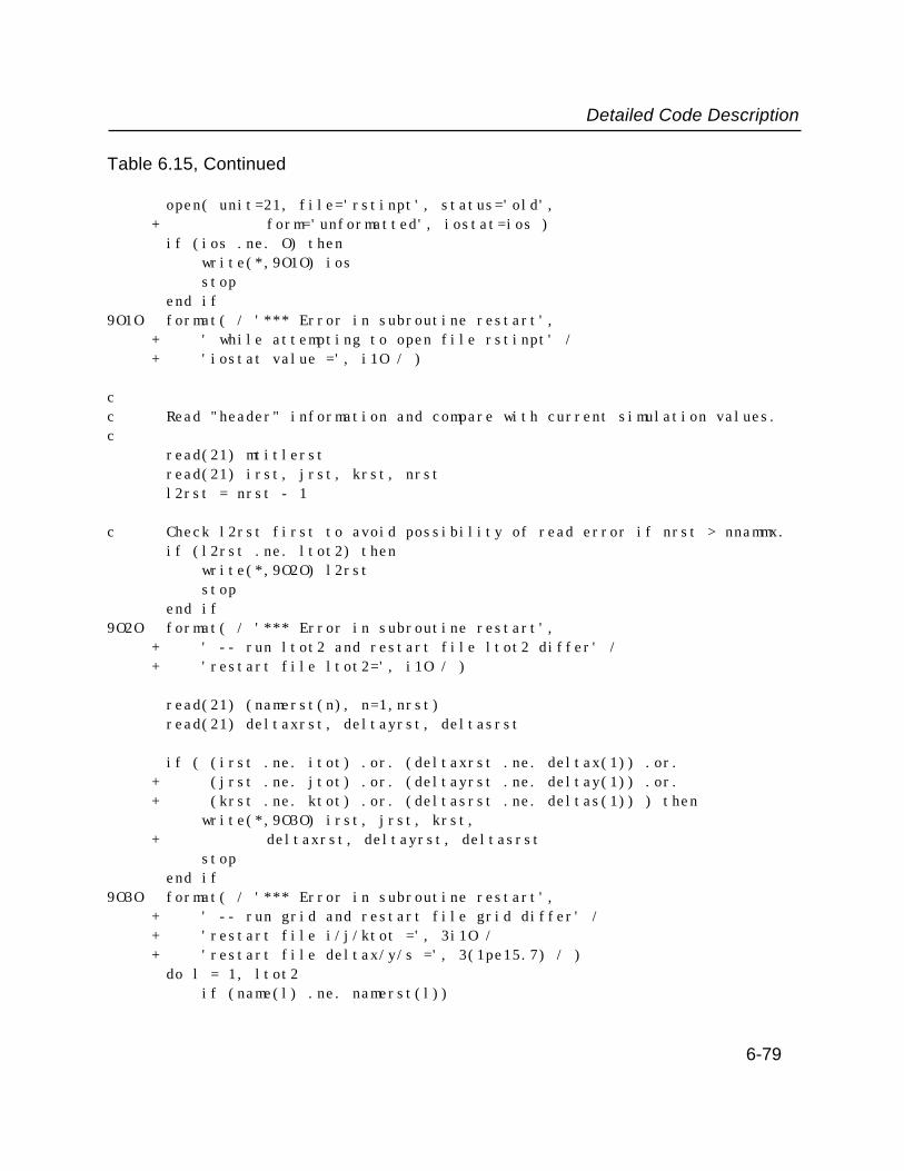
Detailed Code Description
Table 6.15, Continued
open( unit=21, file='rstinpt', status='old', + form='unformatted', iostat=ios )
if (ios .ne. O) then write(*,9O1O) ios stopend if
9O1O format( / '*** Error in subroutine restart', + ' while attempting to open file rstinpt' / + 'iostat value =', i1O / )
cc Read "header" information and compare with current simulation values.c
read(21) mtitlerstread(21) irst, jrst, krst, nrstl2rst = nrst - 1
c Check l2rst first to avoid possibility of read error if nrst > nnammx.if (l2rst .ne. ltot2) then write(*,9O2O) l2rst stopend if
9O2O format( / '*** Error in subroutine restart', + ' -- run ltot2 and restart file ltot2 differ' / + 'restart file ltot2=', i1O / )
read(21) (namerst(n), n=1,nrst)read(21) deltaxrst, deltayrst, deltasrst
if ( (irst .ne. itot) .or. (deltaxrst .ne. deltax(1)) .or. + (jrst .ne. jtot) .or. (deltayrst .ne. deltay(1)) .or. + (krst .ne. ktot) .or. (deltasrst .ne. deltas(1)) ) then
write(*,9O3O) irst, jrst, krst, + deltaxrst, deltayrst, deltasrst
stopend if
9O3O format( / '*** Error in subroutine restart', + ' -- run grid and restart file grid differ' / + 'restart file i/j/ktot =', 3i1O / + 'restart file deltax/y/s =', 3(1pe15.7) / )
do l = 1, ltot2 if (name(l) .ne. namerst(l))
6-79

Detailed Code Description
Table 6.15, Continued
+ write(*,9O4O) l, name(l), namerst(l)end do
9O4O format( '*** subroutine restart -- names differ', + ' -- l, name, namerst = ', i5, 2(3x, a) )cc Read time slices until slice with time = trestart is found.c1OO read(21,end=2OO) t, + ((((r(i,j,k,l), i=1,itot), j=1,jtot), k=1,ktot), l=1,ltot2), + (((cair(i,j,k), i=1,itot), j=1,jtot), k=1,ktot)
if (abs(t-trestart) .le. O.1*dt) then close( unit=21 ) returnelse if (t .lt. trestart) then goto 1OOelse write(*,9O5O) t stopend if
9O5O format( / '*** Error in subroutine restart', + ' -- trestart not found' / + 'last time read from restart file = ', f2O.5 / )2OO write(*,9O6O)
stop9O6O format( / '*** Error in subroutine restart', + ' -- end of file without finding trestart' / )
end
Table 6.16: Listing of Subroutine cloudinit
subroutine cloudinitcc Class II subroutine called from subroutine initc
6-80
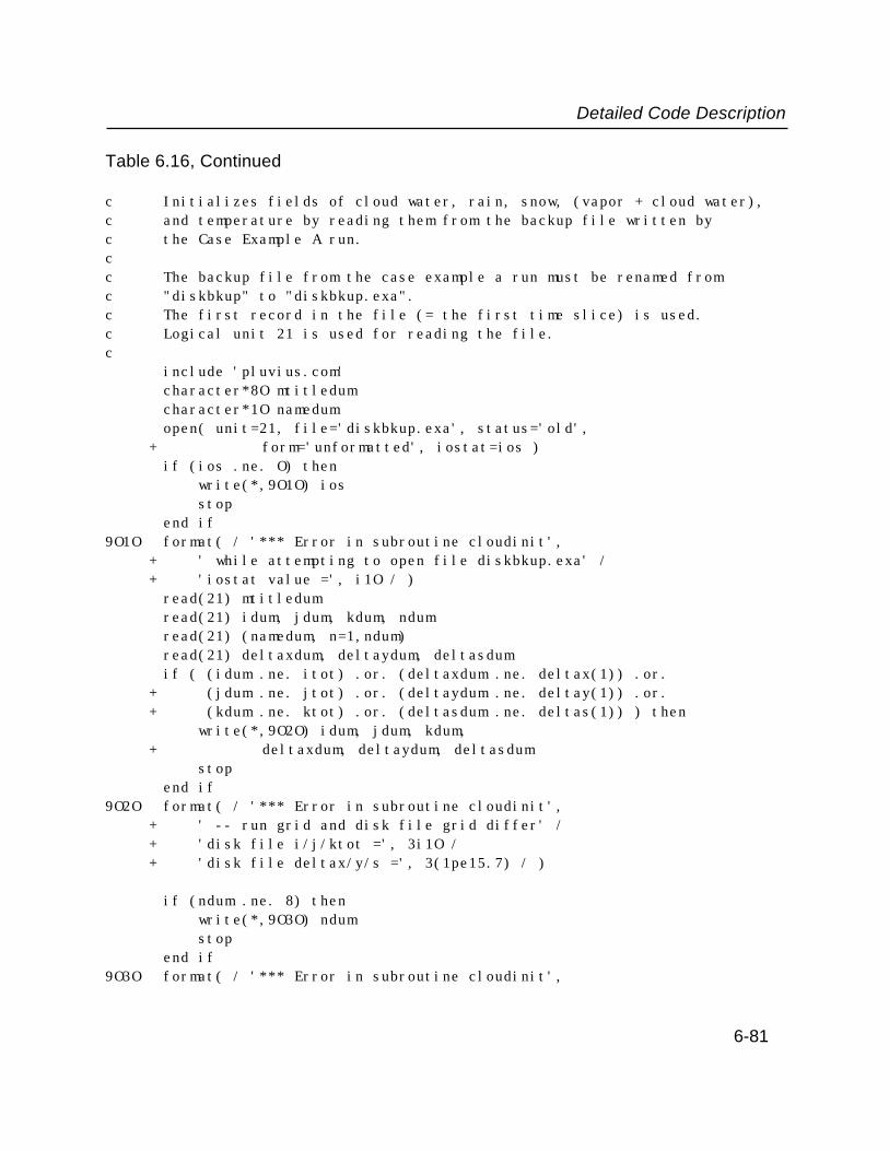
Detailed Code Description
Table 6.16, Continued
c Initializes fields of cloud water, rain, snow, (vapor + cloud water),c and temperature by reading them from the backup file written by c the Case Example A run.cc The backup file from the case example a run must be renamed from c "diskbkup" to "diskbkup.exa".c The first record in the file (= the first time slice) is used.c Logical unit 21 is used for reading the file.c
include 'pluvius.com'character*8O mtitledumcharacter*1O namedumopen( unit=21, file='diskbkup.exa', status='old',
+ form='unformatted', iostat=ios )if (ios .ne. O) then write(*,9O1O) ios stopend if
9O1O format( / '*** Error in subroutine cloudinit', + ' while attempting to open file diskbkup.exa' / + 'iostat value =', i1O / )
read(21) mtitledumread(21) idum, jdum, kdum, ndumread(21) (namedum, n=1,ndum)read(21) deltaxdum, deltaydum, deltasdumif ( (idum .ne. itot) .or. (deltaxdum .ne. deltax(1)) .or.
+ (jdum .ne. jtot) .or. (deltaydum .ne. deltay(1)) .or. + (kdum .ne. ktot) .or. (deltasdum .ne. deltas(1)) ) then
write(*,9O2O) idum, jdum, kdum, + deltaxdum, deltaydum, deltasdum
stopend if
9O2O format( / '*** Error in subroutine cloudinit', + ' -- run grid and disk file grid differ' / + 'disk file i/j/ktot =', 3i1O / + 'disk file deltax/y/s =', 3(1pe15.7) / )
if (ndum .ne. 8) then write(*,9O3O) ndum stopend if
9O3O format( / '*** Error in subroutine cloudinit',
6-81

Detailed Code Description
Table 6.16, Continued
+ ' -- disk file has unexpected number of species =', i1O / )
read(21) tdum, + (((r(i,j,k,lvapcl), i=1,itot), j=1,jtot), k=1,ktot), + (((r(i,j,k,lrain ), i=1,itot), j=1,jtot), k=1,ktot), + (((r(i,j,k,lsnowl), i=1,itot), j=1,jtot), k=1,ktot), + (((rdum, i=1,itot), j=1,jtot), k=1,ktot), + (((r(i,j,k,lcloud), i=1,itot), j=1,jtot), k=1,ktot), + (((rdum, i=1,itot), j=1,jtot), k=1,ktot), + (((r(i,j,k,ltemp ), i=1,itot), j=1,jtot), k=1,ktot), + (((cair(i,j,k), i=1,itot), j=1,jtot), k=1,ktot)
close( unit=21 )
returnend
Table 6.17: Listing of Subroutine inflowinit
subroutine inflowinitcc Class I Subroutine called from subroutine initcc Sets values for mixing ratios (and theta-c) at inflow boundariescc In this version:c The inflow values are set equal to the initial mixing ratios at the c grid point nearest the boundary.c The inflow values are constant in time. If time-varying values are c used, then a different subroutine should be created to calculate (or c read) the time varying values at appropriate time intervals and load c them into the rinflow--- arraysc
include 'pluvius.com'if (mtranx .gt. O) then do 1OO l = 1, ltot do 1OO k = 1, ktot
6-82

Detailed Code Description
Table 6.17, Continued
do 1OO j = 1, jtotrinflowlox(j,k,l) = r(1 ,j,k,l)rinflowhix(j,k,l) = r(itot,j,k,l)
1OO continueend ifif (mtrany .gt. O) then do 2OO l = 1, ltot do 2OO k = 1, ktot do 2OO i = 1, itot
rinflowloy(i,k,l) = r(i,1 ,k,l)rinflowhiy(i,k,l) = r(i,jtot,k,l)
2OO continueend ifif (mtrans .gt. O) then do 3OO l = 1, ltot do 3OO j = 1, jtot do 3OO i = 1, itot
rinflowlos(i,j,l) = r(i,j,1 ,l)rinflowhis(i,j,l) = r(i,j,ktot,l)
3OO continueend ifreturnend
Table 6.18: Listing of Subroutine coreOO
subroutine coreOOcc Class II subroutine called from subroutine corecc Performs some calculations which are only required on very first c call of core in the event that properties computed in the propsx c and/or propsy subroutines are time-invariant. Since vertical c transport properties from propss are computed and storedc for one vertical column at a time, there is no mfreqps=O option.
6-83
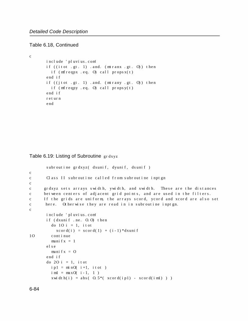
Detailed Code Description
Table 6.18, Continued
c include 'pluvius.com' if ((itot .gt. 1) .and. (mtranx .gt. O)) then if (mfreqpx .eq. O) call propsx(t) end if if ((jtot .gt. 1) .and. (mtrany .gt. O)) then if (mfreqpy .eq. O) call propsy(t) end if return end
Table 6.19: Listing of Subroutine grdxyz
subroutine grdxyz( dxunif, dyunif, dsunif )cc Class II subroutine called from subroutine inptgncc grdxyz sets arrays swidth, ywidth, and xwidth. These are the distancesc between centers of adjacent grid points, and are used in the filters.c If the grids are uniform, the arrays scord, ycord and xcord are also set c here. Otherwise they are read in in subroutine inptgn.c include 'pluvius.com' if (dxunif .ne. O.O) then do 1O i = 1, itot xcord(i) = xcord(1) + (i-1)*dxunif1O continue munifx = 1 else munifx = O end if do 2O i = 1, itot ip1 = minO( i+1, itot ) im1 = maxO( i-1, 1 ) xwidth(i) = abs( O.5*( xcord(ip1) - xcord(im1) ) )
6-84

Detailed Code Description
Table 6.19, Continued
2O continue if (itot .le. 1) xwidth(1) = 1.O if (dyunif .ne. O.O) then do 3O j = 1, jtot ycord(j) = ycord(1) + (j-1)*dyunif3O continue munify = 1 else munify = O end if do 4O j = 1, jtot jp1 = minO( j+1, jtot ) jm1 = maxO( j-1, 1 ) ywidth(j) = abs( O.5*( ycord(jp1) - ycord(jm1) ) )4O continue if (jtot .le. 1) ywidth(1) = 1.O if (dsunif .ne. O.O) then do 5O k = 1, ktot scord(k) = scord(1) + (k-1)*dsunif5O continue munifs = 1 else munifs = O end if do 6O k = 1, ktot kp1 = minO( k+1, ktot ) km1 = maxO( k-1, 1 ) swidth(k) = abs( O.5*( scord(kp1) - scord(km1) ) )6O continue if (ktot .le. 1) swidth(1) = 1.O return end
6-85

Detailed Code Description
Table 6.20: Listing of Subroutine sinteg
subroutine sinteg( minteg, isubt, i, j )cc Class II subroutine called from subroutine corecc Subroutine performs a single integration in the s direction for all c species but at specified i, j.cc Subroutine parameters:c minteg (= 1 or 2) - specifies that this is the first or secondc integration in the 2*dt integration cycle.c isubt - specifies which subintegration core is in.c (minteg and isubt are used in conjunction with control parametersc like mfreqps to determine if physical properties should be c re-calculated).c i, j - the i and j grid points at which the integration is beingc performed.c include 'pluvius.com'cc First set counters for filtering subroutines.c call sfilter( O, O, O, O ) beta = -2./dtcur newcof = O if (mfreqps .eq. O) then write(6,*) 'stop in sinteg: illegal mfreqps', mfreqps pause stop else if (mfreqps .eq. 1) then if ((minteg.eq.1) .and. (isubt.eq.1)) newcof = 1 else if (mfreqps .eq. 1O) then if (minteg .eq. 1) newcof = 1 else if (mfreqps.eq.2O) then newcof = 1 else write(6,*) 'stop in sinteg: illegal mfreqps', mfreqps pause stop end ifcc Compute aas and bbs coeffients for governing equations.c if (newcof .eq. 1) call propss(t,i,j)
6-86

Detailed Code Description
Table 6.20, Continued
cc Compute aas, bbs, and ccs coefficients for minimization integralc (arrays share common names with governing-equation coefficients).c call coefss(newcof, beta, i, j) tbnd=t+O.5*dtcurcc Set boundary conditions.c call bounds(tbnd,i,j,minteg,isubt) do 4O l = 1,ltotcc Load vectors for tridagonal matrix (a, b, c, and d).c call loads(nlo,nhi,i,j,l)cc Solve tridagonal matrix for array v.c call tridag(nlo,nhi,a,b,c,d,v)cc Filter array v.c call sfilter(1,i,j,l) do 3O k = nlo,nhi rclm(k,l) = v(k) 3O continue 4O continue return end
6-87

Detailed Code Description
Table 6.21: Listing of Subroutine propss
subroutine propss(tdum,i,j)cc Class II subroutine called from subroutine sintegc include 'pluvius.com'cc subroutine ***** propss *****cc Supplies "physical properties" in the form of coefficients aas, bbs, andc ccs for the s-components of the governing equations. One interrogation c returns properties corresponding to time tdum for all species and all c vertical points above horizontal position i,j for species equations:cc aas = kzz (generated in subroutine transport)c bbs = - wair - wfall + (kzz/cair) * d(cair)/dzc ccs = -(1./cair) * d(wfall*cair)/dzcc Transport computes vertical transport parameters: fall velocities [in c vertcl(i,j,k,lprops(l))], composite' diffusion coefficients (natural + c differential spread of falling hydrometeors) [in aas(k,lprops(l))]c call transport(i,j)cc Now compute bbs(k,lprops(l)) array.c ds2inv = O.5/deltas(1) do 1O ll = 1,lpstot bbs(1,ll) = aas(1,ll)*(cairclm(2) - cairclm(1)) + /(deltas(1)*cairclm(1)) + -windsclm(1)-vertcclm(1,ll) bbs(ktot,ll) = aas(ktot-1,ll)*(cairclm(ktot)-cairclm(ktot-1)) + /(deltas(ktot-1)*cairclm(ktot)) + -windsclm(ktot)-vertcclm(ktot,ll) ccs(1,ll) = -(cairclm(2)*vertcclm(2,ll)- + cairclm(1)*vertcclm(1,ll))/(deltas(1)*cairclm(1)) ccs(ktot,ll) = -(cairclm(ktot)*vertcclm(ktot,ll)- + cairclm(ktot-1)*vertcclm(ktot-1,ll))/ + (deltas(ktot-1)*cairclm(ktot)) if (munifs .gt. O) thencc case for uniform grid:
6-88

Detailed Code Description
Table 6.21, Continued
c do 2O k = 2,ktot-1 bbs(k,ll) = - windsclm(k) - vertcclm(k,ll) + + O.5*(aas(k,ll) + aas(k-1,ll))* + (cairclm(k+1) - cairclm(k-1))*ds2inv/cairclm(k) ccs(k,ll) = -(cairclm(k+1)*vertcclm(k+1,ll)- + cairclm(k-1)*vertcclm(k-1,ll))*ds2inv/cairclm(k) 2O continue elsecc case for non-uniform grid:c do 3O k = 2, ktot-1 bbs(k,ll) = - windsclm(k) - vertcclm(k,ll) + + O.5*(aas(k,ll) + aas(k-1,ll))* + (fdcofs(1,k)*cairclm(k-1) + + fdcofs(2,k)*cairclm(k ) + + fdcofs(3,k)*cairclm(k+1))/cairclm(k) ccs(k,ll) = + - (fdcofs(1,k)*cairclm(k-1)*vertcclm(k-1,ll) + + fdcofs(2,k)*cairclm(k )*vertcclm(k ,ll) + + fdcofs(3,k)*cairclm(k+1)*vertcclm(k+1,ll)) + /cairclm(k) 3O continue end if 1O continuecc Save values at boundaries (k = 1 and ktot) for possible use with c outflow b. c.'s:c do 4O ll = 1,lpstot asoflo(ll) = O. bsoflo(ll) = -windsclm(1) - vertcclm(1,ll) csoflo(ll) = ccs(1,ll) asofhi(ll) = O. bsofhi(ll) = -windsclm(ktot) - vertcclm(ktot,ll) csofhi(ll) = ccs(ktot,ll)4O continue return end
6-89
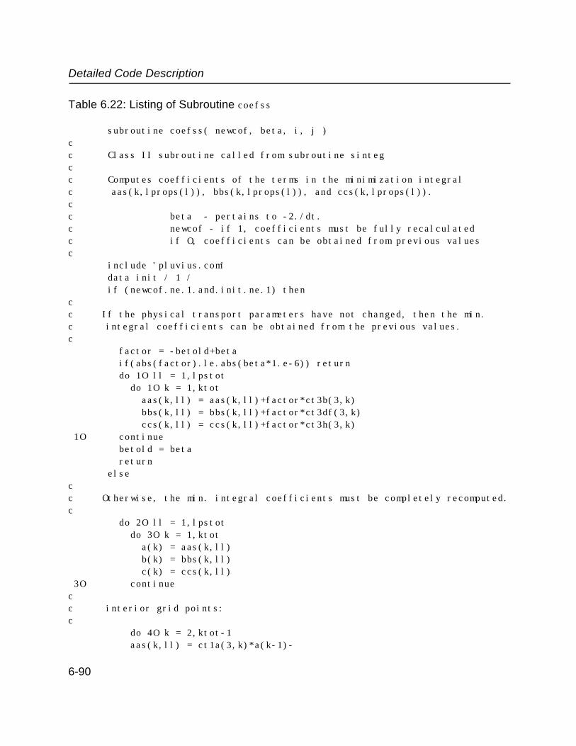
Detailed Code Description
Table 6.22: Listing of Subroutine coefss
subroutine coefss( newcof, beta, i, j )cc Class II subroutine called from subroutine sintegcc Computes coefficients of the terms in the minimization integral c aas(k,lprops(l)), bbs(k,lprops(l)), and ccs(k,lprops(l)).cc beta - pertains to -2./dt.c newcof - if 1, coefficients must be fully recalculatedc if O, coefficients can be obtained from previous valuesc include 'pluvius.com' data init / 1 / if (newcof.ne.1.and.init.ne.1) thencc If the physical transport parameters have not changed, then the min. c integral coefficients can be obtained from the previous values.c factor = -betold+beta if(abs(factor).le.abs(beta*1.e-6)) return do 1O ll = 1,lpstot do 1O k = 1,ktot aas(k,ll) = aas(k,ll)+factor*ct3b(3,k) bbs(k,ll) = bbs(k,ll)+factor*ct3df(3,k) ccs(k,ll) = ccs(k,ll)+factor*ct3h(3,k) 1O continue betold = beta return elsecc Otherwise, the min. integral coefficients must be completely recomputed.c do 2O ll = 1,lpstot do 3O k = 1,ktot a(k) = aas(k,ll) b(k) = bbs(k,ll) c(k) = ccs(k,ll) 3O continuecc interior grid points:c do 4O k = 2,ktot-1 aas(k,ll) = ct1a(3,k)*a(k-1)-
6-90

Detailed Code Description
Table 6.22, Continued
+ .5*b(k-1)+ct3b(3,k)*(c(k-1)+beta) + -ct2a*(b(k)-b(k-1)) + +ct3a(3,k)*(c(k)-c(k-1)) bbs(k,ll) = -ct1a(3,k)*a(k-1)- + ct1c(3,k)*a(k)+ + ct3d(3,k)*(beta+c(k-1))+ + ct3f(3,k)*(beta+c(k)) + -ct2c*(b(k+1)-b(k-1)) + +ct3e(3,k)*(c(k+1)-c(k)) + +ct3c(3,k)*(c(k)-c(k-1)) ccs(k,ll) = +ct1c(3,k)*a(k) + +.5*b(k)+ct3h(3,k)*(c(k)+beta) + +ct2c*(b(k+1)-b(k)) + +ct3e(3,k)*(c(k+1)-c(k)) 4O continue aas(1,ll) = O.O bbs(1,ll) = O.O ccs(1,ll) = O.O aas(ktot,ll) = O.O bbs(ktot,ll) = O.O ccs(ktot,ll) = O.Occ Fill border values for flux b.c.'s:c if (ibclos(ll) .eq. 1) then bbs(1,ll) = -ct1c(3,1)*a(1)-ct2c*(b(2) + -b(1))-.5*b(1)+ct3e(3,1)*(c(2)-c(1))+ + ct3f(3,1)*(c(1)+beta) ccs(1,ll) = ct1c(3,1)*a(1)+ct2c*(b(2) + -b(1))+.5*b(1)+ct3e(3,1)*(c(2)-c(1))+ + ct3h(3,1)*(c(1)+beta) end if if (ibchis(ll) .eq. 1) then aas(ktot,ll) = ct1a(3,ktot)*a(ktot-1) + -ct2a*(b(ktot)-b(ktot-1))-.5*b(ktot-1) + +ct3a(3,ktot)*(c(ktot)-c(ktot-1))+ + ct3b(3,ktot)*(c(ktot-1)+beta) bbs(ktot,ll) = -ct1a(3,ktot)*a(ktot-1) + +ct2a*(b(ktot)-b(ktot-1))+.5*b(ktot-1) + +ct3c(3,ktot)*(c(ktot)-c(ktot-1))+ + ct3d(3,ktot)*(c(ktot-1)+beta) end if
6-91

Detailed Code Description
Table 6.22, Continued
2O continue init = O betold = beta end if return end
Table 6.23: Listing of Subroutine bounds
subroutine bounds(tdum,i,j)cc Class I subroutine called from subroutine sintegcc Computes s-boundary "fluxes" (interpreted here as velocity times mixing c ratio and thus having units of l/t).c include 'pluvius.com'cc For Case Examples A & B the vertical wind component is zero at the topc and bottom boundaries, thus top and bottom fluxes are set to zero atc this point. Transport of precipitation across the bottom boundary isc handled automatically within the numerical integration scheme as anc "outflow" condition.c data ifirst / 1 / do 1OOO l = 1, ltot flxlsclm(l) = O. flxhsclm(l) = O.1OOO continue return end
6-92

Detailed Code Description
Table 6.24: Listing of Subroutine loads
subroutine loads(nlo,nhi,i,j,l)cc Class II subroutine called from subroutine sintegcc Loads elements of tridiagonal matrix for solutions in the s-dimension. c first consolodates coefficients of the integral equations (aas, bbs, c ccs) to obtain internal elements. Then computes boundary conditionsc to obtain external elements.cc Subroutine is called once for each s vector in the domain's matrix.c include 'pluvius.com'
nlo = 1 nhi = ktot ll = lprops(l) do 1O k = 1,ktot a(k) = aas(k,ll) b(k) = bbs(k,ll) c(k) = ccs(k,ll) 1O continuecc compute d array at interior gridsc ktotm1 = ktot - 1 factor = 4./dtcur do 12OO k = 2, ktotm1 d(k) = - (a(k) + factor*ct3b(3,k))*rclm(k-1,l) + - (b(k) + factor*ct3df(3,k))*rclm(k,l) + - (c(k) + factor*ct3h(3,k))*rclm(k+1,l)12OO continuecc Compute d at k=1 boundary, and adjust coefs. for boundary conditions:cc Outflow exists when (windsclm+vertcclm) and deltas have opposite signc (their product is negative);c otherwise inflow or no-flow, in which casec ibclos(ll) = 1 --> flux bcc ibclos(ll) = other --> forced outflow which is treated as zero flux.c k = 1 dumwinds = -bsoflo(ll)
6-93

Detailed Code Description
Table 6.24, Continued
if (dumwinds*deltas(1) .lt. O.O) thenc ( outflow case )c c(1) = bsoflo(ll)/deltas(1) b(1) = -c(1) -1./dtcur + csoflo(ll) a(1) = O. d(1) = -rclm(1,l)/dtcur elsecc ( no outflow )c b(1) = b(1) + bsoflo(ll) d(k) = -(b(k) + factor*ct3df(3,k))*rclm(k,l) + -(c(k) + factor*ct3h(3,k))*rclm(k+1,l) if (ibclos(ll) .eq. 1) d(1) = d(1) - 2.*flxlsclm(l) end ifcc Compute d at k=ktot boundary, & adjust coefs. for boundary conditions.cc Outflow exists when (windsclm+vertcclm) deltas have the same sign c (their product is positive);c otherwise inflow or no-flow, in which casec ibchis(ll) = 1 --> flux bcc ibchis(ll) = other --> forced outflow which is treated as zero flux.c k = ktot dumwinds = -bsofhi(ll) if (dumwinds*deltas(1) .gt. O.O) thencc ( outflow case )c a(ktot) = -bsofhi(ll)/deltas(ktot-1) b(ktot) = -a(ktot) - 1./dtcur + csofhi(ll) c(ktot) = O. d(ktot) = -rclm(ktot,l)/dtcur elsecc ( no outflow )c b(ktot) = b(ktot) - bsofhi(ll) d(k) = - (a(k) + factor*ct3b(3,k))*rclm(k-1,l) + - (b(k) + factor*ct3df(3,k))*rclm(k,l)
6-94

Detailed Code Description
Table 6.24, Continued
if (ibchis(ll) .eq. 1) d(ktot) = d(ktot) + 2.*flxhsclm(l) end if return end
Table 6.25: Listing of Subroutine transport
subroutine transport(i,j)cc Class I subroutine called from subroutines matbal and propsscc Transport computes fall velocities (negative downward) and spread c parameters of rain and snow in cm/sec and cm**2/sec units. Variable c names are vertcclm(k,lprops(lrain)) and vertcclm(k,lprops(lsnow)), c where k is the vertical grid index and lprops denote the transportc regimes.cc include 'pluvius.com' dimension rain(kmaxd),snow(kmaxd),precip(kmaxd) data istart /1/cc Initialize arrays:c if(istart.eq.1) then istart=O do 1O k=1,ktot do 1O l=1,lpsmax vertcclm(k,l)=O. 1O continue end ifcc Define working concentrations in gram-moles per cubic meter.c
6-95

Detailed Code Description
Table 6.25, Continued
do 2O k=1,ktot rain(k)=rclm(k,lrain)*cairclm(k)*1.Oe6 snow(k)=rclm(k,lsnow)*cairclm(k)*1.Oe6 rain(k)=amax1(O.,rain(k)) snow(k)=amax1(O.,snow(k)) precip(k)=rain(k)+snow(k) 2O continuecc Now compute transport properties.c do 3O k=1,ktot drain(k)=3.53*dtcur*rain(k)**.25 dsnow(k)=O.cc drain, dsnow = estimated effective diffusivities of rain & snow arisingc from differential settling velocities, m2/s.c vrain(k)=-O.O1 vsnow(k)=-O.O1c if(precip(k).gt.1.e-5) thencc Compute rain fall velocities in m/s based on Marshall-Palmer c distribution. rlambd is lambda in M-P distribution.c rlambd=1149.*precip(k)**(-.25) aol=1.O2e-3*rlambd eaol=exp(-aol) fact3=1.+aol*(1.+(aol/2.)*(1.+aol/3.)) fact4=1.-eaol*(fact3+(aol**4)/24.) fact3=1.-eaol*fact3 fact34=sqrt(fact3*fact4) vrain(k)=-(1.-fact34)*252.2/sqrt(rlambd)- + 1622O.*fact4/rlambd end ifc if(snow(k).gt.1.e-5) thencc Compute snow fall velocities in m/s based on a Marshall-Palmer c distribution. slambd is lambda in M-P distribution.c tc=rclm(k,ltemp)-273.15
6-96

Detailed Code Description
Table 6.25, Continued
yOflak=5.681e6*exp(-O.O878*amin1(tc,O.)) slambd=2.148*(yOflak/precip(k))**O.3333 aflake=1./slambd vsnow(k)=-4.O6*aflake**.2O6 vbarg=.OO156*aflake**.2O6 if(aflake.lt.3.37e-4) then vsnow(k)=-1296.*aflake**.927 end ifcc Calculate estimated effective snow diffusivity, m2/s.c if(aflake.lt.4.6e-5) vbarg=6.95*aflake**.927 dsnow(k)=dtcur*vbarg*vbarg end if
if(precip(k).gt.O..and.rain(k).gt.O.) + vrain(k)= + (vrain(k)*rain(k) + + vsnow(k)*snow(k))/precip(k) 3O continuecc convert to cm unitsc do 4O k=1,ktot vrain(k)=vrain(k)*1OO. vsnow(k)=vsnow(k)*1OO. drain(k)=difusclm(k,2)+drain(k)*1.Oe4 dsnow(k)=difusclm(k,2)+dsnow(k)*1.Oe4 4O continuecc Do vertical smoothing of rain and snow fallspeeds and diffusivities.c do 5O k=1,ktot-2 vrain(k)=(vrain(k)+vrain(k+1)+vrain(k+2))/3. vsnow(k)=(vsnow(k)+vsnow(k+1)+vsnow(k+2))/3. drain(k)=(drain(k)+drain(k+1)+drain(k+2))/3. dsnow(k)=(dsnow(k)+dsnow(k+1)+dsnow(k+2))/3. 5O continuecc Load vertcclm and aas arraysc do 6O k=1,ktot vertcclm(k,lprops(lrain))=vrain(k)
6-97

Detailed Code Description
Table 6.25, Continued
vertcclm(k,lprops(lsnow))=vsnow(k) aas(k,1)=difusclm(k,1) aas(k,2)=difusclm(k,2) aas(k,lprops(lrain))=drain(k) aas(k,lprops(lsnow))=dsnow(k) 6O continue return end
Table 6.26: Listing of Subroutine xinteg
subroutine xinteg( minteg ) include 'pluvius.com'cc Class II subroutine called from subroutine corecc Subroutine performs a single integration in the x direction.cc minteg (=1 or 2) specifies which integration in the x-y-z-chem-z-y-xc cycle this is.cc First, set counters for filtering subroutinesc call xfilter( O, O, O, O ) beta = -2./dt newcof = O if (mfreqpx .eq. O) then continue else if (mfreqpx .eq. 1) then if (minteg.eq.1) newcof=1 else if(mfreqpx.eq.2) then newcof=1
6-98
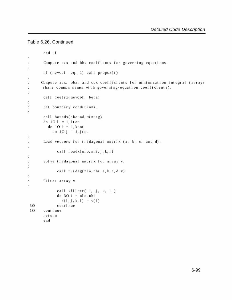
Detailed Code Description
Table 6.26, Continued
end ifcc Compute aax and bbx coeffients for governing equations.c if (newcof .eq. 1) call propsx(t)cc Compute aax, bbx, and ccx coefficients for minimization integral (arraysc share common names with governing-equation coefficients).c call coefsx(newcof, beta)cc Set boundary conditions.c call boundx(tbound,minteg) do 1O l = 1,ltot do 1O k = 1,ktot do 1O j = 1,jtotcc Load vectors for tridagonal matrix (a, b, c, and d).c call loadx(nlo,nhi,j,k,l)cc Solve tridagonal matrix for array v.c call tridag(nlo,nhi,a,b,c,d,v)cc Filter array v.c call xfilter( 1, j, k, l ) do 3O i = nlo,nhi r(i,j,k,l) = v(i) 3O continue 1O continue return end
6-99
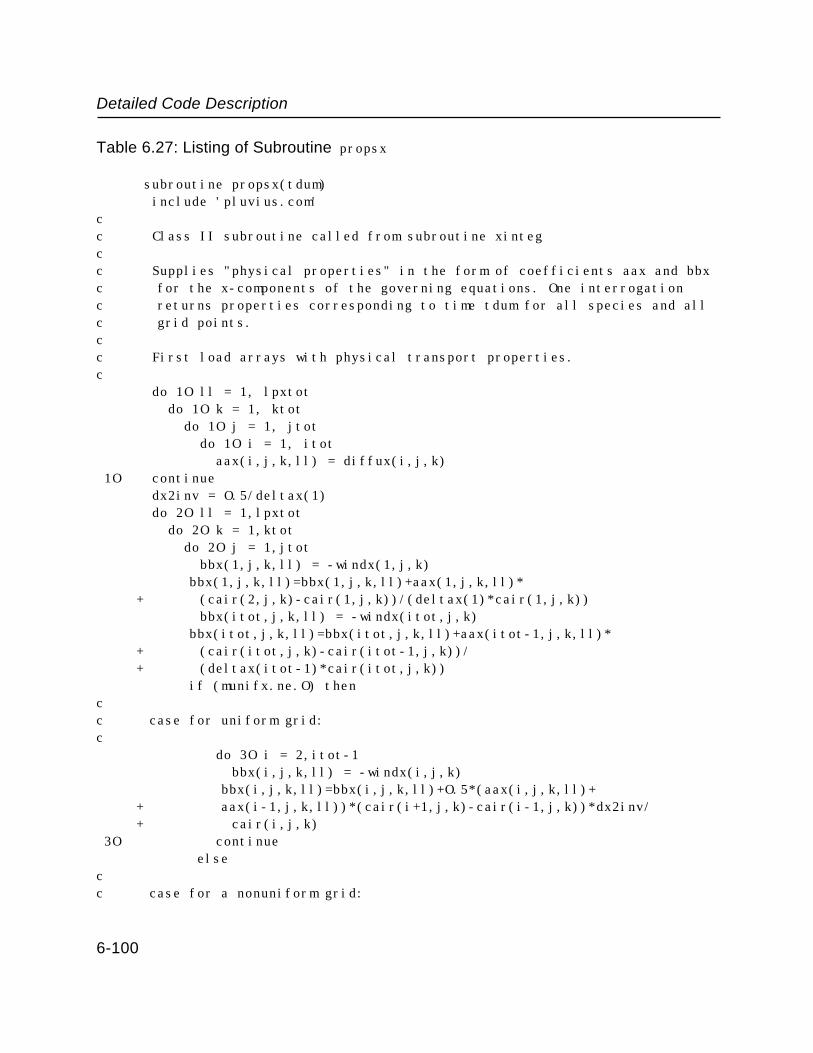
Detailed Code Description
Table 6.27: Listing of Subroutine propsx
subroutine propsx(tdum) include 'pluvius.com'cc Class II subroutine called from subroutine xintegcc Supplies "physical properties" in the form of coefficients aax and bbx c for the x-components of the governing equations. One interrogation c returns properties corresponding to time tdum for all species and all c grid points.cc First load arrays with physical transport properties. c do 1O ll = 1, lpxtot do 1O k = 1, ktot do 1O j = 1, jtot do 1O i = 1, itot aax(i,j,k,ll) = diffux(i,j,k) 1O continue dx2inv = O.5/deltax(1) do 2O ll = 1,lpxtot do 2O k = 1,ktot do 2O j = 1,jtot bbx(1,j,k,ll) = -windx(1,j,k)
bbx(1,j,k,ll)=bbx(1,j,k,ll)+aax(1,j,k,ll)* + (cair(2,j,k)-cair(1,j,k))/(deltax(1)*cair(1,j,k)) bbx(itot,j,k,ll) = -windx(itot,j,k)
bbx(itot,j,k,ll)=bbx(itot,j,k,ll)+aax(itot-1,j,k,ll)* + (cair(itot,j,k)-cair(itot-1,j,k))/ + (deltax(itot-1)*cair(itot,j,k))
if (munifx.ne.O) thencc case for uniform grid:c do 3O i = 2,itot-1 bbx(i,j,k,ll) = -windx(i,j,k)
bbx(i,j,k,ll)=bbx(i,j,k,ll)+O.5*(aax(i,j,k,ll)+ + aax(i-1,j,k,ll))*(cair(i+1,j,k)-cair(i-1,j,k))*dx2inv/ + cair(i,j,k) 3O continue
elsecc case for a nonuniform grid:
6-100

Detailed Code Description
Table 6.27, Continued
c do 4O i=2, itot-1 bbx(i,j,k,ll) = -windx(i,j,k) bbx(i,j,k,ll) = bbx(i,j,k,ll)+
+ O.5*(aax(i,j,k,ll)+aax(i-1,j,k,ll))* + (fdcofx(1,i)*cair(i-1,j,k)+ + fdcofx(2,i)*cair(i,j,k)+ + fdcofx(3,i)*cair(i+1,j,k))/cair(i,j,k) 4O continue
end if 2O continuecc Pack arrays for possible use with outflow b.c.'s.c do 5O ll = 1,lpxtot do 5O k = 1,ktot do 5O j = 1,jtot axoflo(j,k,ll) = O. bxoflo(j,k,ll) = -windx(1,j,k) axofhi(j,k,ll) = O. bxofhi(j,k,ll) = -windx(itot,j,k)5O continue return end
Table 6.28: Listing of Subroutine coefsx
subroutine coefsx( newcof, beta )cc Class II subroutine called from subroutine xintegcc Computes coefficients of terms in the minimization integralc aax(i,j,k,lpropx(l)), bbx(i,j,k,lpropx(l)), and ccx(i,j,k,lpropx(l)).c beta - pertains to -2./dt.
6-101
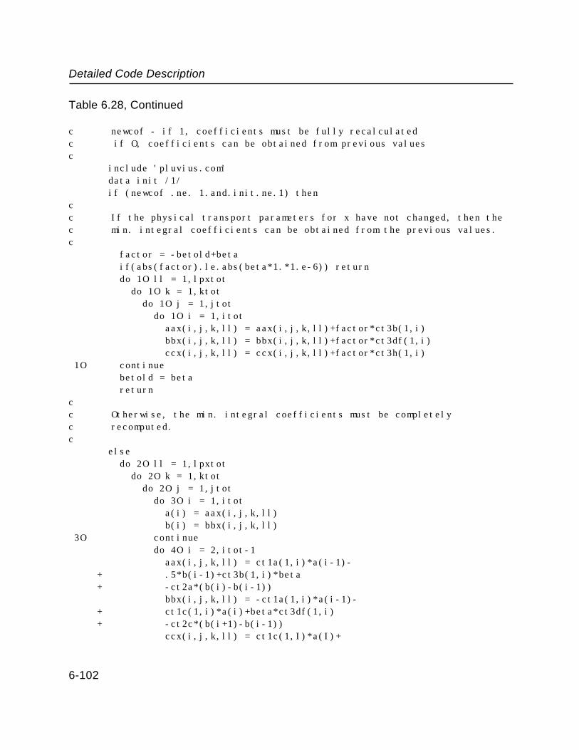
Detailed Code Description
Table 6.28, Continued
c newcof - if 1, coefficients must be fully recalculatedc if O, coefficients can be obtained from previous valuesc include 'pluvius.com' data init /1/ if (newcof .ne. 1.and.init.ne.1) thencc If the physical transport parameters for x have not changed, then the c min. integral coefficients can be obtained from the previous values.c factor = -betold+beta if(abs(factor).le.abs(beta*1.*1.e-6)) return do 1O ll = 1,lpxtot do 1O k = 1,ktot do 1O j = 1,jtot do 1O i = 1,itot aax(i,j,k,ll) = aax(i,j,k,ll)+factor*ct3b(1,i) bbx(i,j,k,ll) = bbx(i,j,k,ll)+factor*ct3df(1,i) ccx(i,j,k,ll) = ccx(i,j,k,ll)+factor*ct3h(1,i) 1O continue betold = beta returncc Otherwise, the min. integral coefficients must be completely c recomputed.c else do 2O ll = 1,lpxtot do 2O k = 1,ktot do 2O j = 1,jtot do 3O i = 1,itot a(i) = aax(i,j,k,ll) b(i) = bbx(i,j,k,ll) 3O continue do 4O i = 2,itot-1 aax(i,j,k,ll) = ct1a(1,i)*a(i-1)- + .5*b(i-1)+ct3b(1,i)*beta + -ct2a*(b(i)-b(i-1)) bbx(i,j,k,ll) = -ct1a(1,i)*a(i-1)- + ct1c(1,i)*a(i)+beta*ct3df(1,i) + -ct2c*(b(i+1)-b(i-1)) ccx(i,j,k,ll) = ct1c(1,I)*a(I)+
6-102
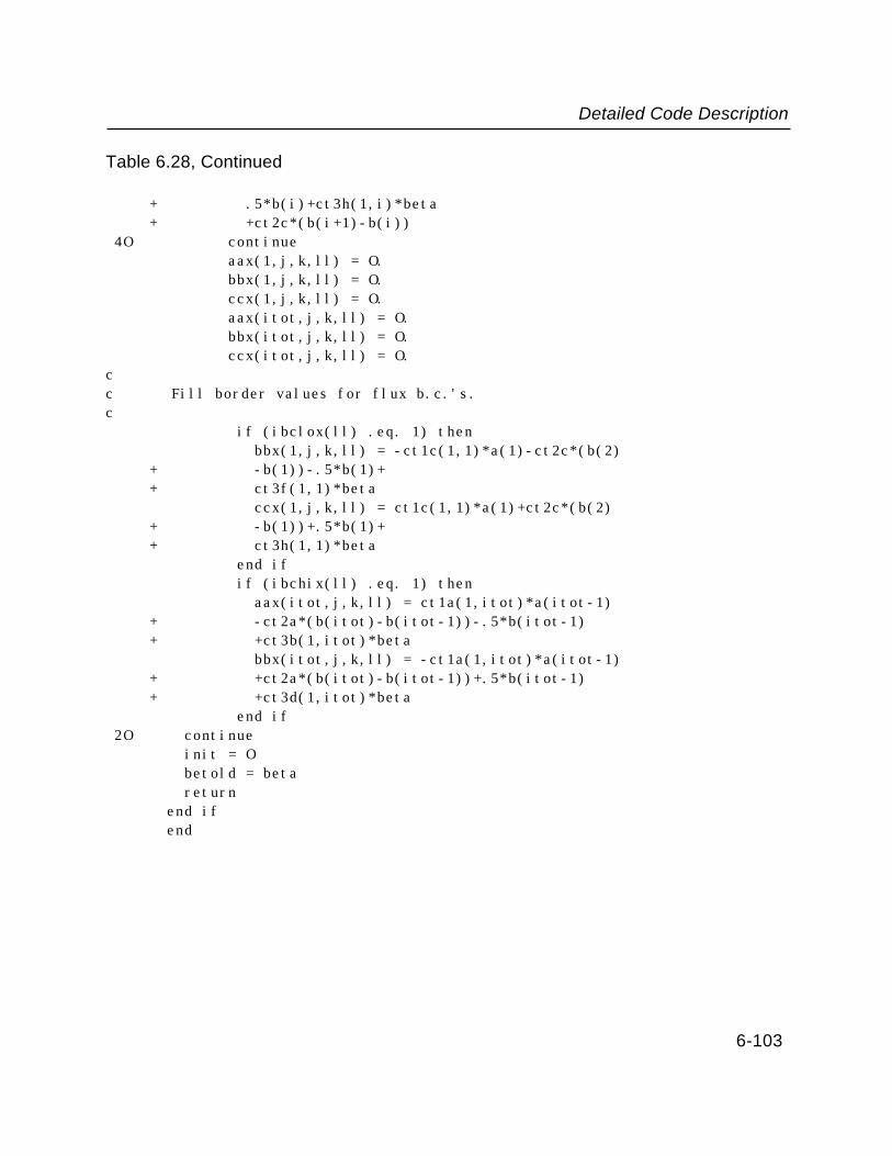
Detailed Code Description
Table 6.28, Continued
+ .5*b(i)+ct3h(1,i)*beta + +ct2c*(b(i+1)-b(i)) 4O continue aax(1,j,k,ll) = O. bbx(1,j,k,ll) = O. ccx(1,j,k,ll) = O. aax(itot,j,k,ll) = O. bbx(itot,j,k,ll) = O. ccx(itot,j,k,ll) = O.cc Fill border values for flux b.c.'s. c if (ibclox(ll) .eq. 1) then bbx(1,j,k,ll) = -ct1c(1,1)*a(1)-ct2c*(b(2) + -b(1))-.5*b(1)+ + ct3f(1,1)*beta ccx(1,j,k,ll) = ct1c(1,1)*a(1)+ct2c*(b(2) + -b(1))+.5*b(1)+ + ct3h(1,1)*beta end if if (ibchix(ll) .eq. 1) then aax(itot,j,k,ll) = ct1a(1,itot)*a(itot-1) + -ct2a*(b(itot)-b(itot-1))-.5*b(itot-1) + +ct3b(1,itot)*beta bbx(itot,j,k,ll) = -ct1a(1,itot)*a(itot-1) + +ct2a*(b(itot)-b(itot-1))+.5*b(itot-1) + +ct3d(1,itot)*beta end if 2O continue init = O betold = beta return end if end
6-103
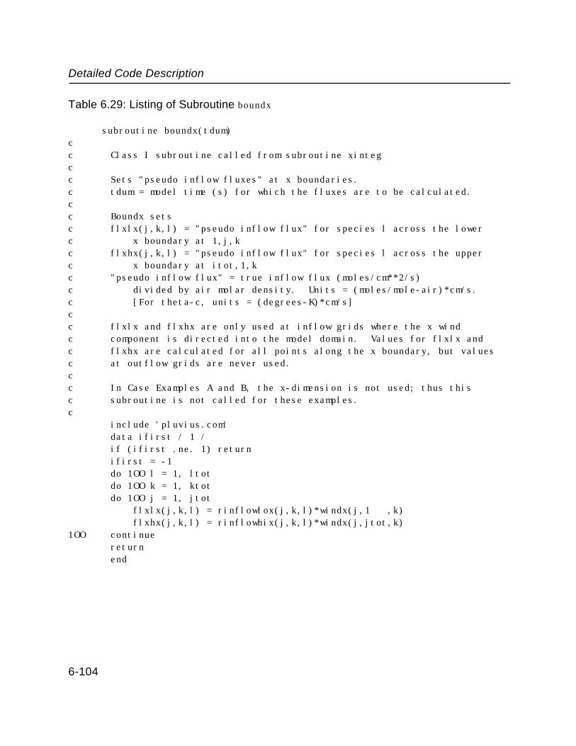
Detailed Code Description
Table 6.29: Listing of Subroutine boundx
subroutine boundx(tdum)cc Class I subroutine called from subroutine xintegcc Sets "pseudo inflow fluxes" at x boundaries.c tdum = model time (s) for which the fluxes are to be calculated.cc Boundx setsc flxlx(j,k,l) = "pseudo inflow flux" for species l across the lowerc x boundary at 1,j,kc flxhx(j,k,l) = "pseudo inflow flux" for species l across the upperc x boundary at itot,1,kc "pseudo inflow flux" = true inflow flux (moles/cm**2/s)c divided by air molar density. Units = (moles/mole-air)*cm/s.c [For theta-c, units = (degrees-K)*cm/s]cc flxlx and flxhx are only used at inflow grids where the x wind c component is directed into the model domain. Values for flxlx and c flxhx are calculated for all points along the x boundary, but values c at outflow grids are never used.cc In Case Examples A and B, the x-dimension is not used; thus this c subroutine is not called for these examples.c
include 'pluvius.com'data ifirst / 1 /if (ifirst .ne. 1) returnifirst = -1do 1OO l = 1, ltotdo 1OO k = 1, ktotdo 1OO j = 1, jtot flxlx(j,k,l) = rinflowlox(j,k,l)*windx(j,1 ,k) flxhx(j,k,l) = rinflowhix(j,k,l)*windx(j,jtot,k)
1OO continuereturnend
6-104
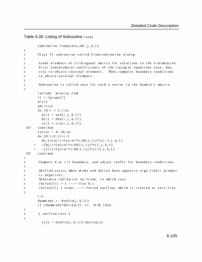
Detailed Code Description
Table 6.30: Listing of Subroutine loadx
subroutine loadx(nlo,nhi,j,k,l)cc Class II subroutine called from subroutine xintegcc Loads elements of tridiagonal matrix for solutions in the x-dimension. c First consolodates coefficients of the integral equations (aax, bbx, c ccx) to obtain internal elements. Then computes boundary conditions c to obtain external elements. cc Subroutine is called once for each x vector in the domain's matrix.c include 'pluvius.com' ll = lpropx(l) nlo=1 nhi=itot do 1O i = 1,itot a(i) = aax(i,j,k,ll) b(i) = bbx(i,j,k,ll) c(i) = ccx(i,j,k,ll) 1O continue factor = 4./dtcur do 2O i=2,itit-1 d(i)=(a(i)+factor*ct3b(1,i))*r(i-1,j,k,l) + -(b(i)+factor*ct3df(1,i))*r(i,j,k,l) + -(c(i)+factor*ct3h(1,i))*r(i+1,j,k,l) 2O continuecc Compute d at i=1 boundary, and adjust coeffs for boundary conditions.cc Outflow exists when windx and deltax have opposite sign (their product c is negative).c Otherwise inflow (or no flow), in which casec ibclox(ll) = 1 ---> flux b.c.c ibclox(ll) = other ---> forced outflow, which is treated as zero flux.c i=1 dumwindx = -bxoflo(j,k,ll) if (dumwindx*deltax(1) .lt. O.O) thencc ( outflow case )c c(1) = bxoflo(j,k,ll)/deltax(1)
6-105

Detailed Code Description
Table 6.30, Continued
b(1) = -c(1) - 1./dtcur a(1) = O. d(1) = -r(1,j,k,l)/dtcur else cc ( no outflow )c b(1) = b(1) - windx(1,j,k) d(i) = - (b(i) + factor*ct3df(1,i))*r(i,j,k,l) + -(c(i) + factor*ct3h(1,i)) *r(i+1,j,k,l) if (ibclos(ll) .eq. 1) d(i) = d(i) - 2.*flxlx(j,k,l) end ifcc Compute d at i=itot boundary, and adjust coefs. for bound. conditions.cc Outflow exists when windx and deltax have the same sign (their product c is positive).c Otherwise inflow or no-flow, in which casec ibchix(ll) = 1 --> flux bcc ibchix(ll) = other --> forced outflow which is treated as zero flux.c i = itot dumwindx = -bxofhi(j,k,ll) if (dumwindx*deltax(1) .gt. O.O) thencc ( outflow case )c a(itot) = -bxofhi(j,k,ll)/deltax(itot-1) b(itot) = -a(itot) - 1./dtcur c(itot) = O. d(itot) = -r(itot,j,k,l)/dtcur else cc ( no outflow )c b(itot) = b(itot) + windx(itot,j,k) d(i) = - (a(i) + factor*ct3b(1,i))*r(i-1,j,k,l) + -(b(i) + factor*ct3df(1,i))*r(i,j,k,l) if (ibchix(ll) .eq. 1) d(i) = d(i) + 2.*flxhx(j,k,l) end if return end
6-106

Detailed Code Description
Table 6.31: Listing of Subroutine yinteg
subroutine yinteg( minteg ) include 'pluvius.com'cc Class II subroutine called from subroutine corecc Subroutine performs a single integration in the y direction.cc minteg (=1 or 2) - specifies which integration this is in the c x-y-z-chem-z-y-x integration cycle.cc First set counters for filtering subroutines.c call yfilter( O, O, O, O ) beta = -2./dt newcof=O if (mfreqpy .eq. O) then continue else if (mfreqpy .eq. 1) then if(minteg.eq.1) newcof=1 else if (mfreqpy.eq.2) then newcof = 1 end ifcc Compute aay and bby coeffients for governing equations.c if (newcof .eq. 1) call propsy(t)cc Compute aay, bby, and ccy coefficients for minimization integral c (arrays share common names with governing-equation coefficients).c call coefsy(newcof, beta) tbnd=t+.5*dtcc Set boundary conditions.c call boundy(tbnd,minteg) do 1O l = 1,ltot do 1O k = 1,ktot do 1O i = 1,itotcc Load vectors for tridagonal matrix (a, b, c, and d).c
6-107
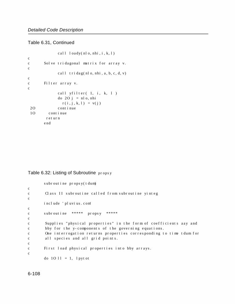
Detailed Code Description
Table 6.31, Continued
call loady(nlo,nhi,i,k,l)cc Solve tridagonal matrix for array v.c call tridag(nlo,nhi,a,b,c,d,v)cc Filter array v.c call yfilter( 1, i, k, l ) do 2O j = nlo,nhi r(i,j,k,l) = v(j) 2O continue 1O continue return end
Table 6.32: Listing of Subroutine propsy
subroutine propsy(tdum)cc Class II subroutine called from subroutine yintegc include 'pluvius.com'cc subroutine ***** propsy *****cc Supplies "physical properties" in the form of coefficients aay and c bby for the y-components of the governing equations.c One interrogation returns properties corresponding to time tdum for c all species and all grid points.cc First load physical properties into bby arrays. c do 1O ll = 1, lpytot
6-108

Detailed Code Description
Table 6.32, Continued
do 1O k = 1, ktot do 1O j = 1, jtot do 1O i = 1, itot aay(i,j,k,ll) = diffuy(i,j,k) 1O continue dy2inv = O.5/deltay(1) do 2O ll = 1,lpytot do 2O k = 1,ktot do 2O i = 1,itotcc Set bby at boundaries:c bby(i,1,k,ll) = -windy(i,1,k)
bby(i,1,k,ll)=bby(i,1,k,ll)+aay(i,1,k,ll)* + (cair(i,2,k)-cair(i,1,k))/(deltay(1)*cair(i,1,k)) bby(i,jtot,k,ll) = -windy(i,jtot,k)
bby(i,jtot,k,ll)=bby(i,jtot,k,ll)+aay(i,jtot-1,k,ll)* + (cair(i,jtot,k)-cair(i,jtot-1,k))/ + (deltay(jtot-1)*cair(i,jtot,k))cc Now set bby for internal points:c
if (munify.gt.O) thencc case for a uniform gridc do 3O j = 2,jtot-1 bby(i,j,k,ll) = -windy(i,j,k)
bby(i,j,k,ll)=bby(i,j,k,ll)+O.5*(aay(i,j,k,ll)+ + aay(i,j-1,k,ll))*(cair(i,j+1,k)-cair(i,j-1,k))* + dy2inv/cair(i,j,k) 3O continue
elsecc case for a nonuniform gridc
do 4O j=2, jtot-1 bby(i,j,k,ll) = -windy(i,j,k) bby(i,j,k,ll) = bby(i,j,k,ll)+
+ O.5*(aay(i,j,k,ll)+aay(i,j-1,k,ll))* + (fdcofy(1,j)*cair(i,j-1,k)+ + fdcofy(2,j)*cair(i,j,k)+
6-109
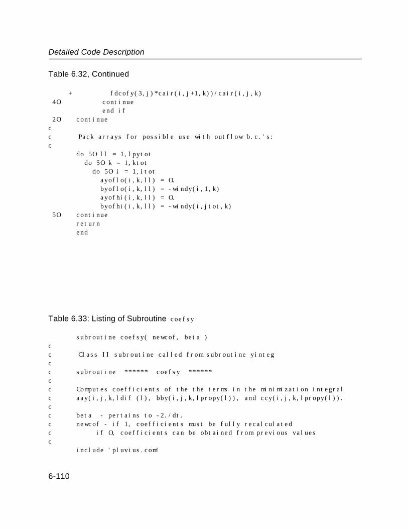
Detailed Code Description
Table 6.32, Continued
+ fdcofy(3,j)*cair(i,j+1,k))/cair(i,j,k) 4O continue
end if 2O continuecc Pack arrays for possible use with outflow b.c.'s:c do 5O ll = 1,lpytot do 5O k = 1,ktot do 5O i = 1,itot ayoflo(i,k,ll) = O. byoflo(i,k,ll) = -windy(i,1,k) ayofhi(i,k,ll) = O. byofhi(i,k,ll) = -windy(i,jtot,k) 5O continue return end
Table 6.33: Listing of Subroutine coefsy
subroutine coefsy( newcof, beta )cc Class II subroutine called from subroutine yintegcc subroutine ****** coefsy ******cc Computes coefficients of the the terms in the minimization integralc aay(i,j,k,ldif (l), bby(i,j,k,lpropy(l)), and ccy(i,j,k,lpropy(l)).cc beta - pertains to -2./dt.c newcof - if 1, coefficients must be fully recalculatedc if O, coefficients can be obtained from previous valuesc include 'pluvius.com'
6-110
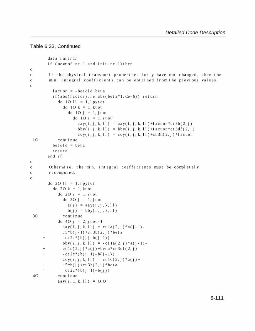
Detailed Code Description
Table 6.33, Continued
data init/1/ if (newcof.ne.1.and.init.ne.1)thencc If the physical transport properties for y have not changed, then the c min. integral coefficients can be obtained from the previous values.c factor = -betold+beta if(abs(factor).le.abs(beta*1.Oe-6)) return do 1O ll = 1,lpytot do 1O k = 1,ktot do 1O j = 1,jtot do 1O i = 1,itot aay(i,j,k,ll) = aay(i,j,k,ll)+factor*ct3b(2,j) bby(i,j,k,ll) = bby(i,j,k,ll)+factor*ct3df(2,j) ccy(i,j,k,ll) = ccy(i,j,k,ll)+ct3h(2,j)*factor 1O continue betold = beta return end ifcc Otherwise, the min. integral coefficients must be completely c recomputed.c do 2O ll = 1,lpytot do 2O k = 1,ktot do 2O i = 1,itot do 3O j = 1,jtot a(j) = aay(i,j,k,ll) b(j) = bby(i,j,k,ll) 3O continue do 4O j = 2,jtot-1 aay(i,j,k,ll) = ct1a(2,j)*a(j-1)- + .5*b(j-1)+ct3b(2,j)*beta + -ct2a*(b(j)-b(j-1)) bby(i,j,k,ll) = -ct1a(2,j)*a(j-1)- + ct1c(2,j)*a(j)+beta*ct3df(2,j) + -ct2c*(b(j+1)-b(j-1)) ccy(i,j,k,ll) = ct1c(2,j)*a(j)+ + .5*b(j)+ct3h(2,j)*beta + +ct2c*(b(j+1)-b(j)) 4O continue aay(i,1,k,ll) = O.O
6-111
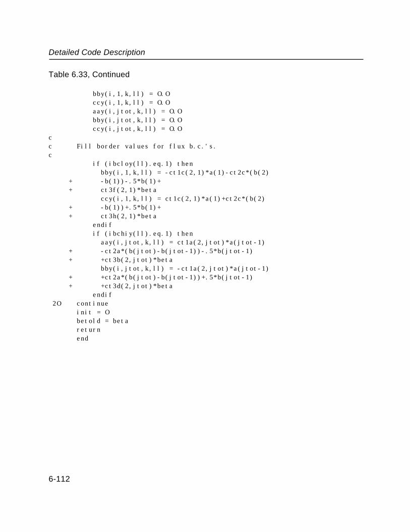
Detailed Code Description
Table 6.33, Continued
bby(i,1,k,ll) = O.O ccy(i,1,k,ll) = O.O aay(i,jtot,k,ll) = O.O bby(i,jtot,k,ll) = O.O ccy(i,jtot,k,ll) = O.Occ Fill border values for flux b.c.'s.c if (ibcloy(ll).eq.1) then bby(i,1,k,ll) = -ct1c(2,1)*a(1)-ct2c*(b(2) + -b(1))-.5*b(1)+ + ct3f(2,1)*beta ccy(i,1,k,ll) = ct1c(2,1)*a(1)+ct2c*(b(2) + -b(1))+.5*b(1)+ + ct3h(2,1)*beta endif if (ibchiy(ll).eq.1) then aay(i,jtot,k,ll) = ct1a(2,jtot)*a(jtot-1) + -ct2a*(b(jtot)-b(jtot-1))-.5*b(jtot-1) + +ct3b(2,jtot)*beta bby(i,jtot,k,ll) = -ct1a(2,jtot)*a(jtot-1) + +ct2a*(b(jtot)-b(jtot-1))+.5*b(jtot-1) + +ct3d(2,jtot)*beta endif 2O continue init = O betold = beta return end
6-112

Detailed Code Description
Table 6.34: Listing of Subroutine boundy
subroutine boundy( tdum )cc Class I subroutine called from subroutine yintegcc Sets "pseudo inflow fluxes" at y boundaries.c tdum = model time (s) for which the fluxes are to be calculatedcc boundy sets:c flxly(i,k,l) = "pseudo inflow flux" for species l across the lowerc y boundary at i,1,k.c flxhy(i,k,l) = "pseudo inflow flux" for species l across the upperc y boundary at i,jtot,k.c "pseudo inflow flux" = true inflow flux (moles/cm**2/s)c divided by air molar density. Units = (moles/mole-air)*cm/s.c [For theta-c, units = (degrees-K)*cm/s]cc flxly and flxhy are only used at inflow grids where the y wind c component is directed in to the model domain. Values for flxly and c flxhy are calculated for all points along the y boundary, but values c at outflow grids are never used.cc In Case Examples A and B, both the winds and the inflow mixing ratiosc are constant in time, so flxly and flxhy are also constant in time.c
include 'pluvius.com'data ifirst / 1 /if (ifirst .ne. 1) returnifirst = -1do 1OO l = 1, ltotdo 1OO k = 1, ktotdo 1OO i = 1, itot flxly(i,k,l) = rinflowloy(i,k,l)*windy(i,1 ,k) flxhy(i,k,l) = rinflowhiy(i,k,l)*windy(i,jtot,k)
1OO continuereturnend
6-113
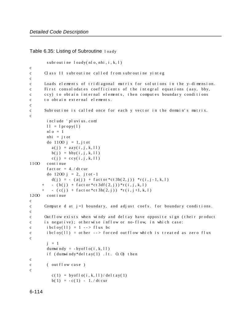
Detailed Code Description
Table 6.35: Listing of Subroutine loady
subroutine loady(nlo,nhi,i,k,l)cc Class II subroutine called from subroutine yintegcc Loads elements of tridiagonal matrix for solutions in the y-dimension. c First consolodates coefficients of the integral equations (aay, bby, c ccy) to obtain internal elements, then computes boundary conditionsc to obtain external elements.cc Subroutine is called once for each y vector in the domain's matrix.c include 'pluvius.com' ll = lpropy(l) nlo = 1 nhi = jtot do 11OO j = 1,jtot a(j) = aay(i,j,k,ll) b(j) = bby(i,j,k,ll) c(j) = ccy(i,j,k,ll)11OO continue factor = 4./dtcur do 12OO j = 2, jtot-1 d(j) = - (a(j) + factor*ct3b(2,j)) *r(i,j-1,k,l) + - (b(j) + factor*ct3df(2,j))*r(i,j,k,l) + - (c(j) + factor*ct3h(2,j)) *r(i,j+1,k,l)12OO continuecc Compute d at j=1 boundary, and adjust coefs. for boundary conditions.cc Outflow exists when windy and deltay have opposite sign (their product c is negative); otherwise inflow or no-flow, in which case:c ibcloy(ll) = 1 --> flux bcc ibcloy(ll) = other --> forced outflow which is treated as zero fluxc j = 1 dumwindy = -byoflo(i,k,ll) if (dumwindy*deltay(1) .lt. O.O) thencc ( outflow case )c c(1) = byoflo(i,k,ll)/deltay(1) b(1) = -c(1) - 1./dtcur
6-114

Detailed Code Description
Table 6.35, Continued
a(1) = O. d(1) = -r(i,1,k,l)/dtcur else cc ( no outflow ) b(1) = b(1) - windy(i,1,k) d(j) = - (b(j) + factor*ct3df(2,j))*r(i,j,k,l) + - (c(j) + factor*ct3h(2,j)) *r(i,j+1,k,l) if (ibcloy(ll) .eq. 1) d(j) = d(j) - 2.*flxly(i,k,l) end ifcc Compute d at j=jtot boundary, and adjust coefs. for boundary conditions.cc Outflow exists when windy and deltay have the same signc (their product is positive)c Otherwise inflow or no-flow, in which case:c ibchiy(ll) = 1 --> flux bcc ibchiy(ll) = other --> forced outflow which is treated as zero fluxc j = jtot dumwindy = -byofhi(i,k,ll) if (dumwindy*deltay(1) .gt. O.O) thencc ( outflow case )c a(jtot) = -byofhi(i,k,ll)/deltay(jtot-1) b(jtot) = -a(jtot) - 1./dtcur c(jtot) = O. d(jtot) = -r(i,jtot,k,l)/dtcur else cc ( no outflow )c b(jtot) = b(jtot) + windy(i,jtot,k) d(j) = - (a(j) + factor*ct3b(2,j)) *r(i,j-1,k,l) + - (b(j) + factor*ct3df(2,j))*r(i,j,k,l) if (ibchiy(ll) .eq. 1) d(j) = d(j) + 2.*flxhy(i,k,l) end if return end
6-115
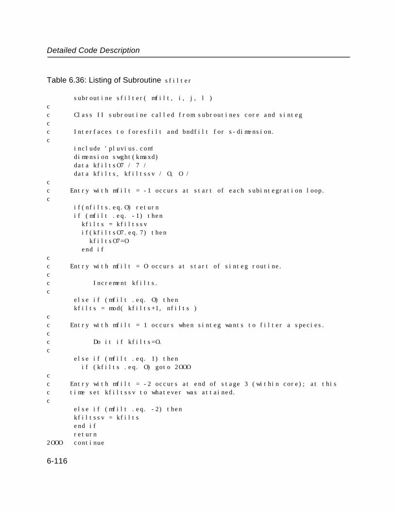
Detailed Code Description
Table 6.36: Listing of Subroutine sfilter
subroutine sfilter( mfilt, i, j, l )cc Class II subroutine called from subroutines core and sintegcc Interfaces to foresfilt and bndfilt for s-dimension.c include 'pluvius.com' dimension swght(kmaxd) data kfiltsO7 / 7 / data kfilts, kfiltssv / O, O /cc Entry with mfilt = -1 occurs at start of each subintegration loop.c if(nfilts.eq.O) return if (mfilt .eq. -1) then kfilts = kfiltssv if(kfiltsO7.eq.7) then kfiltsO7=O end ifcc Entry with mfilt = O occurs at start of sinteg routine.cc Increment kfilts.c else if (mfilt .eq. O) then kfilts = mod( kfilts+1, nfilts )cc Entry with mfilt = 1 occurs when sinteg wants to filter a species.cc Do it if kfilts=O.c else if (mfilt .eq. 1) then if (kfilts .eq. O) goto 2OOOcc Entry with mfilt = -2 occurs at end of stage 3 (within core); at this c time set kfiltssv to whatever was attained.c else if (mfilt .eq. -2) then kfiltssv = kfilts end if return2OOO continue
6-116

Detailed Code Description
Table 6.36, Continued
do 2O1O k=1,ktot swght(k)=cairclm(k)*swidth(k) 2O1O continue filfac=filfacs(1) if(filfac.le.O) returncc First filter boundary values if inflow.c lpss = lprops(l) if (mbndfils .gt. O) go to 21OO pecle1 = (windsclm(1) + vertcclm(1,lpss)) + *deltas(1)/amax1( 1.e-1O, difusclm(1,1) ) peclen = (windsclm(ktot) + vertcclm(ktot,lpss)) + *deltas(ktot-1)/amax1( 1.e-1O, difusclm(ktot,1) ) call bndfilt( v, ktot, pecle1, peclen,swght,filfac)cc Then do the rest.c 21OO continue courno = O.O filfac = filfacs(l) call foresfilt( v, ktot, filfac,nfilsrch,nfiltset, + nfiltitr,swght) return end
Table 6.37: Listing of Subroutine xfilter
subroutine xfilter( mfilt, j, k, l )cc Class II subroutine called from subroutine xintegcc Interfaces to foresfilt and bndfilt for x-dimension.c include 'pluvius.com'
6-117
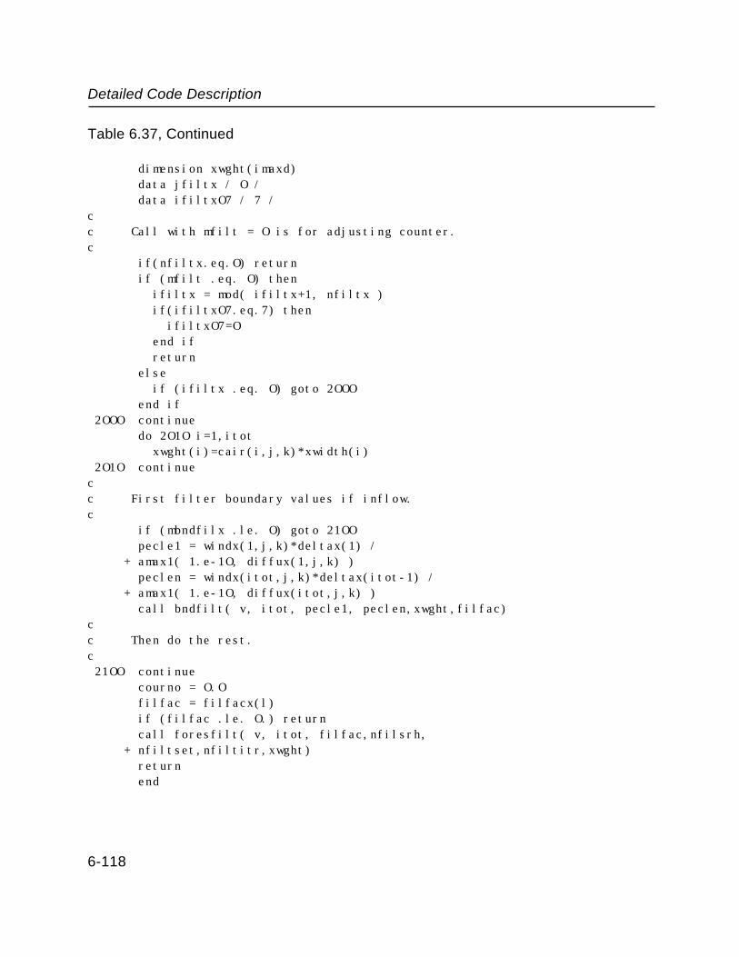
Detailed Code Description
Table 6.37, Continued
dimension xwght(imaxd) data jfiltx / O / data ifiltxO7 / 7 /cc Call with mfilt = O is for adjusting counter.c if(nfiltx.eq.O) return if (mfilt .eq. O) then ifiltx = mod( ifiltx+1, nfiltx ) if(ifiltxO7.eq.7) then ifiltxO7=O end if return else if (ifiltx .eq. O) goto 2OOO end if 2OOO continue do 2O1O i=1,itot xwght(i)=cair(i,j,k)*xwidth(i) 2O1O continuecc First filter boundary values if inflow.c if (mbndfilx .le. O) goto 21OO pecle1 = windx(1,j,k)*deltax(1) / + amax1( 1.e-1O, diffux(1,j,k) ) peclen = windx(itot,j,k)*deltax(itot-1) / + amax1( 1.e-1O, diffux(itot,j,k) ) call bndfilt( v, itot, pecle1, peclen,xwght,filfac)cc Then do the rest.c 21OO continue courno = O.O filfac = filfacx(l) if (filfac .le. O.) return call foresfilt( v, itot, filfac,nfilsrh, + nfiltset,nfiltitr,xwght) return end
6-118
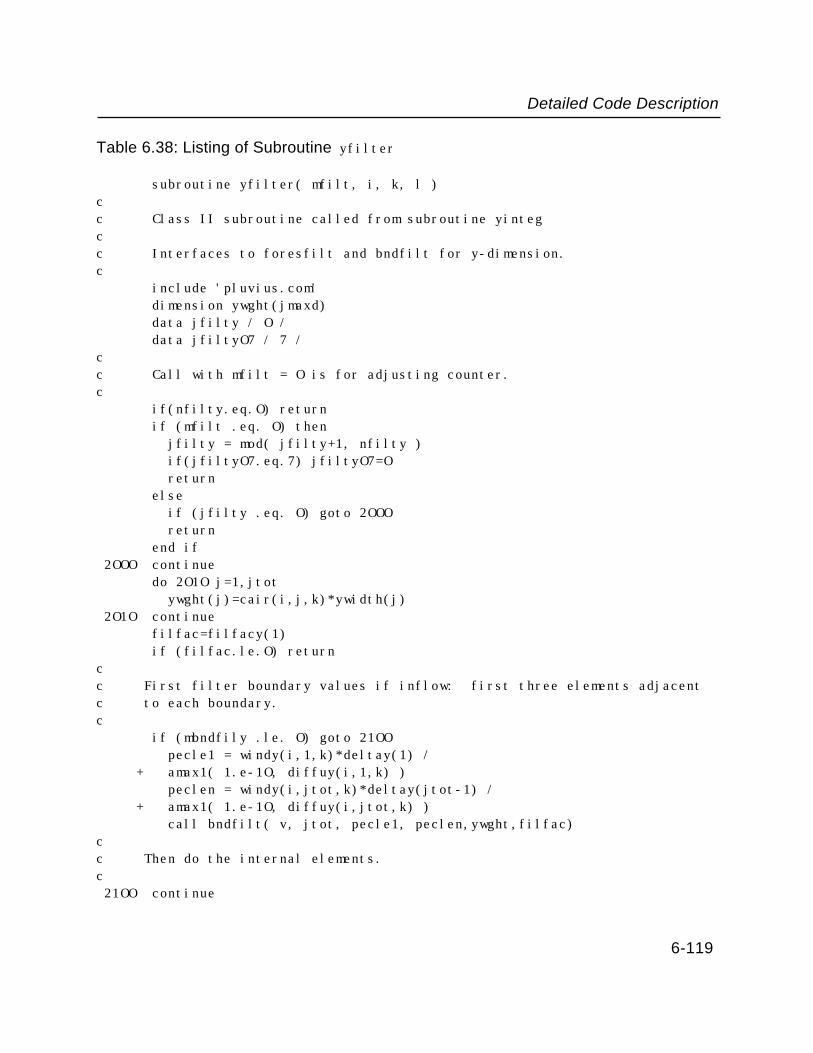
Detailed Code Description
Table 6.38: Listing of Subroutine yfilter
subroutine yfilter( mfilt, i, k, l )cc Class II subroutine called from subroutine yintegcc Interfaces to foresfilt and bndfilt for y-dimension.c include 'pluvius.com' dimension ywght(jmaxd) data jfilty / O / data jfiltyO7 / 7 /cc Call with mfilt = O is for adjusting counter.c if(nfilty.eq.O) return if (mfilt .eq. O) then jfilty = mod( jfilty+1, nfilty ) if(jfiltyO7.eq.7) jfiltyO7=O return else if (jfilty .eq. O) goto 2OOO return end if 2OOO continue do 2O1O j=1,jtot ywght(j)=cair(i,j,k)*ywidth(j) 2O1O continue filfac=filfacy(1) if (filfac.le.O) returncc First filter boundary values if inflow: first three elements adjacent c to each boundary.c if (mbndfily .le. O) goto 21OO pecle1 = windy(i,1,k)*deltay(1) / + amax1( 1.e-1O, diffuy(i,1,k) ) peclen = windy(i,jtot,k)*deltay(jtot-1) / + amax1( 1.e-1O, diffuy(i,jtot,k) ) call bndfilt( v, jtot, pecle1, peclen,ywght,filfac)cc Then do the internal elements.c 21OO continue
6-119
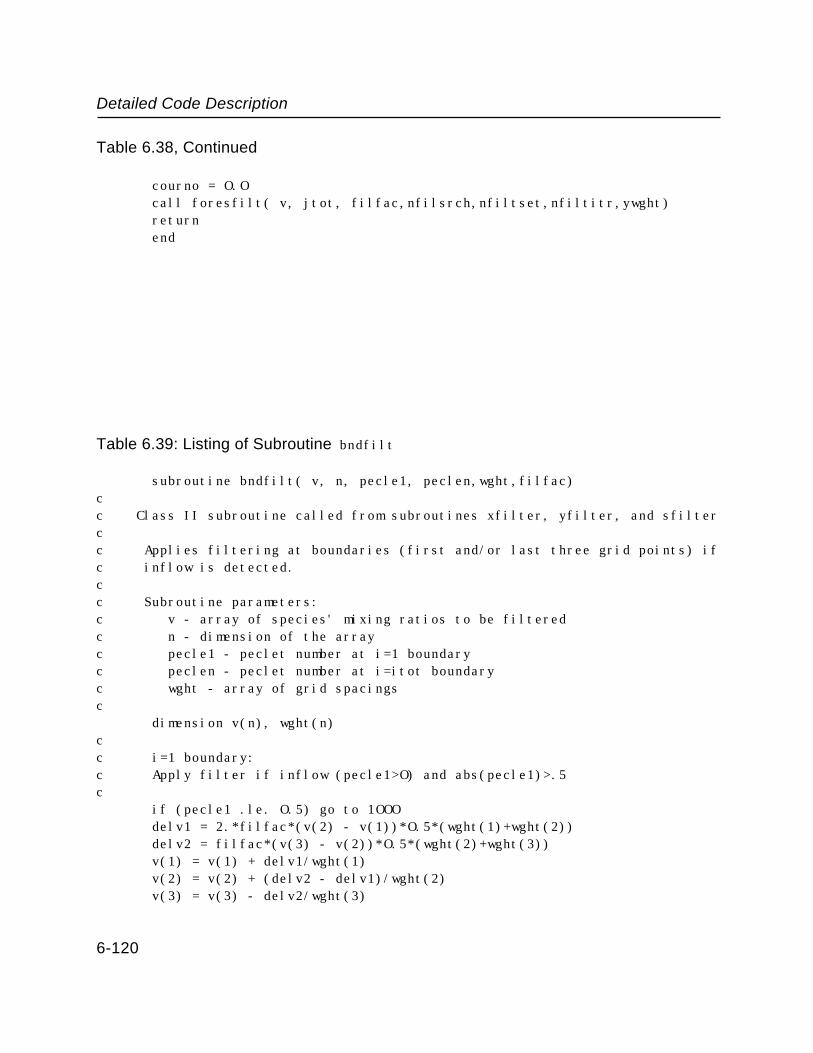
Detailed Code Description
Table 6.38, Continued
courno = O.O call foresfilt( v, jtot, filfac,nfilsrch,nfiltset,nfiltitr,ywght) return end
Table 6.39: Listing of Subroutine bndfilt
subroutine bndfilt( v, n, pecle1, peclen,wght,filfac)cc Class II subroutine called from subroutines xfilter, yfilter, and sfiltercc Applies filtering at boundaries (first and/or last three grid points) ifc inflow is detected.cc Subroutine parameters:c v - array of species' mixing ratios to be filteredc n - dimension of the arrayc pecle1 - peclet number at i=1 boundaryc peclen - peclet number at i=itot boundaryc wght - array of grid spacingsc dimension v(n), wght(n)cc i=1 boundary:c Apply filter if inflow (pecle1>O) and abs(pecle1)>.5c if (pecle1 .le. O.5) go to 1OOO delv1 = 2.*filfac*(v(2) - v(1))*O.5*(wght(1)+wght(2)) delv2 = filfac*(v(3) - v(2))*O.5*(wght(2)+wght(3)) v(1) = v(1) + delv1/wght(1) v(2) = v(2) + (delv2 - delv1)/wght(2) v(3) = v(3) - delv2/wght(3)
6-120

Detailed Code Description
Table 6.39, Continued
cc i=n boundary:c Apply filter if inflow (peclen<O) and abs(pecle1)>.5c 1OOO if (peclen .ge. -O.5) goto 2OOO delvn = 2.*filfac*(v(n) - v(n-1))*.5*(wght(n)+wght(n-1)) delvnm1 = filfac*(v(n-1) - v(n-2))*.5*(wght(n-1)+wght(n-2)) v(n) = v(n) - delvn/wght(n) v(n-1) = v(n-1) + (delvn - delvnm1)/wght(n-1) v(n-2) = v(n-2) + delvnm1/wght(n-2) 2OOO return end
Table 6.40: Listing of Subroutine foresfilt
subroutine foresfilt(c,n,filfac,nfsrch,nfset,maxitr,wght)cc Class II subroutine called from subroutines xfilter, yfilter, and sfiltercc Applies non-linear filter of C.K.Forester (j.comp.phys, 1977, pp 1-22).cc---------------------------------------------------------------------------cc Subroutine parameters:c c - one dimensional array of values to be filteredc n - the number of valuesc filfac - the filter factor =O.5*mu in Forester's paperc specified by user for each species. suggested values arec O.1 for filtered species, O.O for non-filtered speciesc wght - one-dimensional array of grid weightsc wght(i)= air density * grid width
nfsrch, nfset - n and m of Forester's paper. A value that is ac local maximum (or minimum) is considered to be a true c extremum if it exceeds the nfsrch adjacent values. Otherwisec it is treated as "noise," and filtering is applied to it and c the nset adjacent values.
6-121
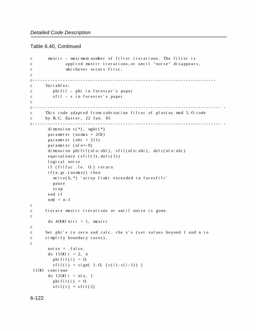
Detailed Code Description
Table 6.40, Continued
c maxitr - maximum number of filter iterations. The filter is c applied maxitr iterations,or until "noise" disappears, c whichever occurs first.cc-------------------------------------------------------------------------c Variables:c phifil - phi in forester's paperc sfil - s in forester's papercc--------------------------------------------------------------------------- -c This code adapted from subroutine filter of pluvius mod 5.O codec by R.C. Easter, 22 Jan. 85c--------------------------------------------------------------------------- - dimension c(*), wght(*) parameter (nzmax = 2O1) parameter (nhi = 211) parameter (nlo=-9) dimension phifil(nlo:nhi), sfil(nlo:nhi), delc(nlo:nhi) equivalence (sfil(1),delc(1)) logical noise if (filfac .le. O.) return if(n.gt.(nzmax)) then write(6,*) 'array limit exceeded in foresfilt' pause stop end if nm1 = n-1cc Iterate maxitr iterations or until noise is gone.c do 4OOO nitr = 1, maxitrcc Set phi's to zero and calc. the s's (set values beyond 1 and n to c simplify boundary cases).c noise = .false. do 11OO i = 2, n phifil(i) = O. sfil(i) = sign( 1.O, (c(i)-c(i-1)) ) 11OO continue do 12OO i = nlo, 1 phifil(i) = O. sfil(i) = sfil(2)
6-122
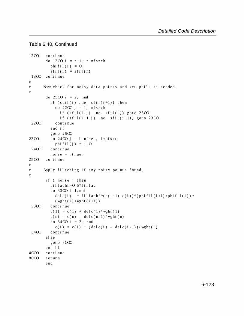
Detailed Code Description
Table 6.40, Continued
12OO continue do 13OO i = n+1, n+nfsrch phifil(i) = O. sfil(i) = sfil(n) 13OO continuecc Now check for noisy data points and set phi's as needed.c do 25OO i = 2, nm1 if (sfil(i) .ne. sfil(i+1)) then do 22OO j = 1, nfsrch if (sfil(i-j) .ne. sfil(i)) goto 23OO if (sfil(i+1+j) .ne. sfil(i+1)) goto 23OO 22OO continue end if goto 25OO23OO do 24OO j = i-nfset, i+nfset phifil(j) = 1.O 24OO continue noise = .true.25OO continuecc Apply filtering if any noisy points found.c if ( noise ) then filfachf=O.5*filfac do 33OO i=1,nm1 delc(i) = filfachf*(c(i+1)-c(i))*(phifil(i+1)+phifil(i))* + (wght(i)+wght(i+1)) 33OO continue c(1) = c(1) + delc(1)/wght(1) c(n) = c(n) - delc(nm1)/wght(n) do 34OO i = 2, nm1 c(i) = c(i) + (delc(i) - delc(i-1))/wght(i) 34OO continue else goto 8OOO end if4OOO continue8OOO return end
6-123
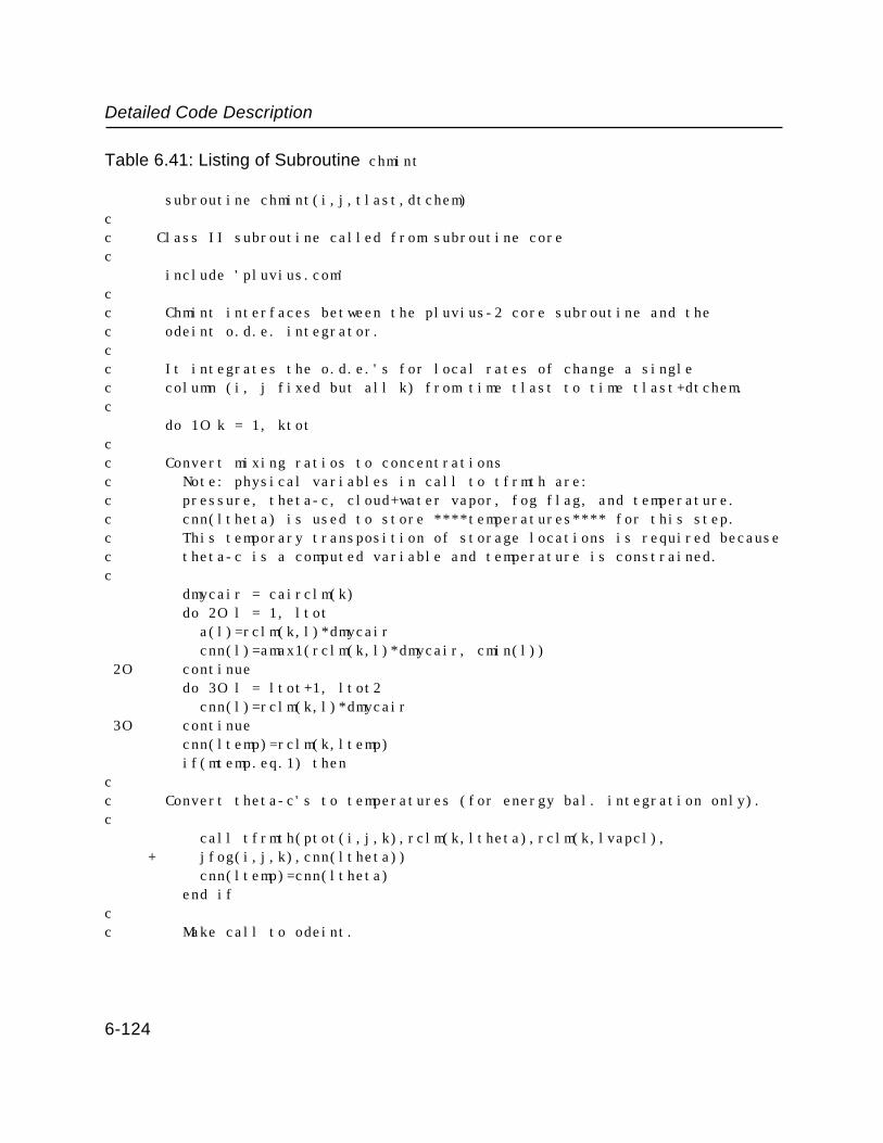
Detailed Code Description
Table 6.41: Listing of Subroutine chmint
subroutine chmint(i,j,tlast,dtchem)cc Class II subroutine called from subroutine corec include 'pluvius.com'cc Chmint interfaces between the pluvius-2 core subroutine and thec odeint o.d.e. integrator.cc It integrates the o.d.e.'s for local rates of change a singlec column (i, j fixed but all k) from time tlast to time tlast+dtchem.c do 1O k = 1, ktotcc Convert mixing ratios to concentrationsc Note: physical variables in call to tfrmth are:c pressure, theta-c, cloud+water vapor, fog flag, and temperature.c cnn(ltheta) is used to store ****temperatures**** for this step.c This temporary transposition of storage locations is required because c theta-c is a computed variable and temperature is constrained.c dmycair = cairclm(k) do 2O l = 1, ltot a(l)=rclm(k,l)*dmycair cnn(l)=amax1(rclm(k,l)*dmycair, cmin(l)) 2O continue do 3O l = ltot+1, ltot2 cnn(l)=rclm(k,l)*dmycair 3O continue cnn(ltemp)=rclm(k,ltemp) if(mtemp.eq.1) thencc Convert theta-c's to temperatures (for energy bal. integration only).c call tfrmth(ptot(i,j,k),rclm(k,ltheta),rclm(k,lvapcl), + jfog(i,j,k),cnn(ltheta)) cnn(ltemp)=cnn(ltheta) end ifcc Make call to odeint.
6-124

Detailed Code Description
Table 6.41, Continued
dtsug = dtsave(i,j,k) call odeint(i,j, k, tlast, dtchem, dtsug, dtchem ) dtsave(i,j,k) = dtsugcc convert back to mixing ratiosc if initial conc. was below cmin, adjust downwardsc do 4O l = 1, ltot if(a(l).lt.cmin(l)) cnn(l) = cnn(l) +a(l) -cmin(l) rclm(k,l) = cnn(l)/dmycair 4O continue do 5O l = ltot+1, ltot2 rclm(k,l) = cnn(l)/dmycair 5O continue
rclm(k,ltemp)=cnn(ltemp) if(mtemp.eq.1) thencc Convert temperatures back to theta-c's.c
rclm(k,ltheta)=(1.e6/ptot(i,j,k))**ak*(cnn(ltheta)- + alocp*rclm(k,lcloud)) end if 1O continue return end
Table 6.42: Listing of Subroutine odeint
subroutine odeint(i,j,k,tstrto, dttot, dtsug, dtmax )cc Class II subroutine called from subroutine chmintc include "pluvius.com"
6-125

Detailed Code Description
Table 6.42, Continued
c----------------------------------------------------------------------cc subroutine ***** odeint *****cc Performs numerical integrations of the system of equationscc d( c(k,l) )/dt = ggen(l) - gdec(l)cc where:c t is the independent variablec c(k,l) is the vector of dependent variables (k is fixedc during each call to odeint)c ggen(l) is the vector of species generation ratesc gdec(l) is the vector of species destruction rates.c (gdec(l) is expressed internally as a psuedo c first-order relation gdec(l) = xi(l)*c(l), where xi(l) c is the vector of psuedo first-order rate coefficients.cc Both ggen(l) and gdec(l) are determined by interrogating a user-suppliedc subroutine, named gen.ccc tstrto is the model time at the begining of the call to odeint.cc dttot is the time interval over which the equations are integrated.cc dtmax is the (user specified) maximum allowable time step.cc dtsug is the "suggested" initial time step for the integration. If this c is set negative by the calling program, then odeint will determine its c own step size. (after a successful integration, the final step size isc passed back in dtsave(i,j,k). It should be used to establish c dtsug on repeated calls.)cc-------------------------------------------------------------------cc The following parameters affect the mechanics of the numericalc integration. they are held in common blocks, and should be initialized c in the setup subroutine.cc ncorr is the desired number of corrector passes per time step. (**an c odd number is recommended**).
6-126

Detailed Code Description
Table 6.42, Continued
cc iexp determines stiff integration method: "asymptotic" (iexp = O),c or "exponentially assisted" (iexp = 1).cc cmin = values of dependent variables, below which they can be c considered as insignificant to the overall computation. Must be c set as positive, non-zero numbers prior to subroutine call.cc cerror = values of dependent variables, below which the convergence c error criterion is relaxed. Must be set as positive, non-zero c numbers prior to subroutine call. Typically, one should set c cmin(k) < .OO1*cerror(k).cc eps = maximum allowable normalized disagreement between the c predictor and corrector, or between successive corrector cycles; c i. e., maximum convergence error.cc ratesf = values of psuedo first-order decay coefficient above which c the corresponding equations are considered stiff. This parameter c can be adjusted to optimize computationalefficiency of the c algorithm. For typical air chemistry problems, a suggested value c is .O1 sec(-1).c c dtmin = minimum allowable step sizecc----------------------------------------------------------------------
dimension stiff(lmaxd), ffp(lmaxd), cstart(l2maxd), + ggenp(lmaxd), xi(lmaxd), xip(lmaxd), pred(lmaxd)cc Initialize variables and flags.cc iflg = terminal increment flag; = 1 when on last c timestep of integration.c tn = current value of dependent variable.c dtrem = remaining span to be integrated.c iflg = O tn = tstrto ts = tstrto dtrem = dttot pfact = 1.
6-127
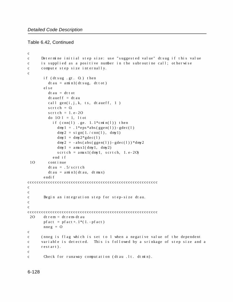
Detailed Code Description
Table 6.42, Continued
cc Determine initial step size: use "suggested value" dtsug if this value c is supplied as a positive number in the subroutine call; otherwise c compute step size internally.c if (dtsug .gt. O.) then dtau = amin1(dtsug, dttot) else dtau = dttot dtaueff = dtau call gen(i,j,k, ts, dtaueff, 1 ) scrtch = O. scrtch = 1.e-2O do 1O l = 1, ltot if (cnn(l) .ge. 1.1*cmin(l)) then dmy1 = .1*eps*abs(ggen(l))-gdec(l) dmy2 = sign(1./cnn(l), dmy1) dmy1 = dmy2*gdec(l) dmy2 = -abs(abs(ggen(l))-gdec(l))*dmy2 dmy1 = amax1(dmy1, dmy2) scrtch = amax1(dmy1, scrtch, 1.e-2O) end if 1O continue dtau = .5/scrtch dtau = amin1(dtau, dtmax) endifcccccccccccccccccccccccccccccccccccccccccccccccccccccccccccc Begin an integration step for step-size dtau.ccccccccccccccccccccccccccccccccccccccccccccccccccccccccccc 2O dtrem = dtrem-dtau pfact = pfact+.1*(1.-pfact) nneg = Occ (nneg is flag which is set to 1 when a negative value of the dependent c variable is detected. This is followed by a srinkage of step size and ac restart).cc Check for runaway computation (dtau .lt. dtmin).
6-128
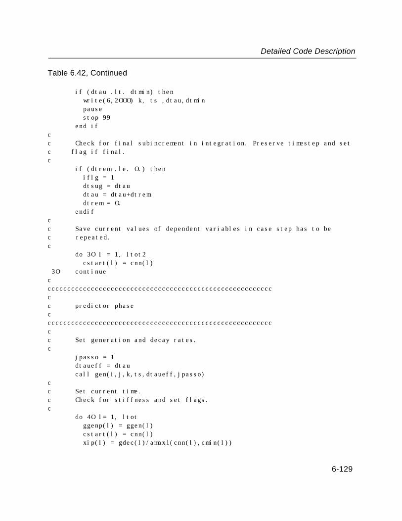
Detailed Code Description
Table 6.42, Continued
if (dtau .lt. dtmin) then write(6,2OOO) k, ts ,dtau,dtmin pause stop 99 end ifcc Check for final subincrement in integration. Preserve timestep and set c flag if final.c if (dtrem .le. O.) then iflg = 1 dtsug = dtau dtau = dtau+dtrem dtrem = O. endifcc Save current values of dependent variables in case step has to be c repeated.c do 3O l = 1, ltot2 cstart(l) = cnn(l) 3O continuecccccccccccccccccccccccccccccccccccccccccccccccccccccccccccc predictor phasecccccccccccccccccccccccccccccccccccccccccccccccccccccccccccc Set generation and decay rates. c jpasso = 1 dtaueff = dtau call gen(i,j,k,ts,dtaueff,jpasso)cc Set current time. c Check for stiffness and set flags.c do 4O l= 1, ltot ggenp(l) = ggen(l) cstart(l) = cnn(l) xip(l) = gdec(l)/amax1(cnn(l),cmin(l))
6-129
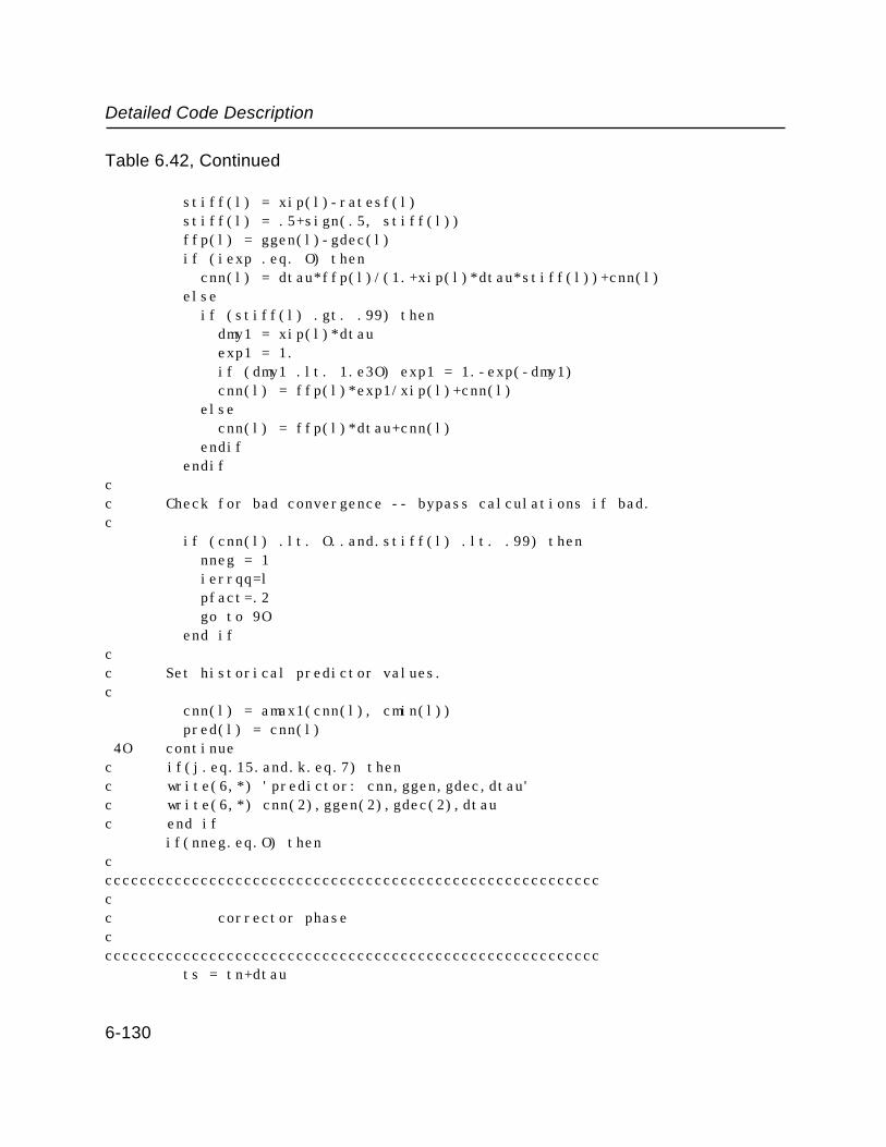
Detailed Code Description
Table 6.42, Continued
stiff(l) = xip(l)-ratesf(l) stiff(l) = .5+sign(.5, stiff(l)) ffp(l) = ggen(l)-gdec(l) if (iexp .eq. O) then cnn(l) = dtau*ffp(l)/(1.+xip(l)*dtau*stiff(l))+cnn(l) else if (stiff(l) .gt. .99) then dmy1 = xip(l)*dtau exp1 = 1. if (dmy1 .lt. 1.e3O) exp1 = 1.-exp(-dmy1) cnn(l) = ffp(l)*exp1/xip(l)+cnn(l) else cnn(l) = ffp(l)*dtau+cnn(l) endif endifcc Check for bad convergence -- bypass calculations if bad.c if (cnn(l) .lt. O..and.stiff(l) .lt. .99) then nneg = 1 ierrqq=l pfact=.2 go to 9O end ifcc Set historical predictor values.c cnn(l) = amax1(cnn(l), cmin(l)) pred(l) = cnn(l) 4O continuec if(j.eq.15.and.k.eq.7) thenc write(6,*) 'predictor: cnn,ggen,gdec,dtau'c write(6,*) cnn(2),ggen(2),gdec(2),dtauc end if if(nneg.eq.O) thencccccccccccccccccccccccccccccccccccccccccccccccccccccccccccc corrector phasecccccccccccccccccccccccccccccccccccccccccccccccccccccccccc ts = tn+dtau
6-130

Detailed Code Description
Table 6.42, Continued
do 6O icorr=1,ncorr jpasso = jpasso + 1 call gen(i,j,k,ts, dtaueff, jpasso ) do 7O l = 1, ltot xi(l) = gdec(l)/amax1(cnn(l),cmin(l)) xim = .5*(xip(l)+xi(l)) ggenm = .5*(ggen(l)+ggenp(l)) if (stiff(l) .lt. .99) thencc Not stiff; use conventional Euler's method.c cnn(l) = cstart(l)+dtau*(ggenm-.5*xim*(cnn(l)+cstart(l)))cc Check for bad convergence; bypass calculations if bad.c if (cnn(l) .lt. O..and.stiff(l) .lt. .99) then nneg = 1 ierrqq=l pfact=.2 go to 9O end if elsecc Stiff; use exponential approximation.c if (iexp .eq. O) thencc Use asymptotic form.c dmy1 = dtau*(1.+.5*xim*dtau) cnn(l) = cstart(l)+(ggenm-cstart(l)*xim)* + dmy1/(1.+xim*dmy1) elsecc Use exponential formc dmy1 = xim*dtau exp1 = 1. if (dmy1 .lt. 1.e3O) exp1 = 1.-exp(-dmy1) cnn(l) = (ggenm/xim-cstart(l))*exp1+cstart(l) end if end if
6-131

Detailed Code Description
Table 6.42, Continued
cnn(l) = amax1(cnn(l), cmin(l)) 7O continue 6O continuec if(j.eq.15.and.k.eq.7) thenc write(6,*) 'corrector: cnn,ggen,gdec,dtau ='c write(6,*) cnn(2),ggen(2),gdec(2),dtauc pausec end ifcccccccccccccccccccccccccccccccccccccccccccccccccccccccccccc error check and step size adjustmentcccccccccccccccccccccccccccccccccccccccccccccccccccccccccccc Basic convergence criterion is:c abs( (predictor-corrector)/corrector ) < epscc The convergence criterion is relaxed under a number of circumstances. c This error relaxation should be considered "application-dependent", and c the user may wish to modify it as required. in the air-chemistry c applications of the Pluvius Mod 5 users' manual, errors are relaxed c whenever:c 1) concentrations approach negligible values (rlocon)c 2) the starting concentration is negligibly small (rzrost)c 3) the projected increase is so large as to make the currentc value and its relative error small by comparison (rfasti)c 4) the projected decrease is rapid (rfastd)cc Set minimum value of errmxc errmx = 1.e-6cc Setting minimum errmx to 1.e-6 limits step size increase to c sqrt(1.e6*eps).c do 8O l = 1, ltot rlocon = O.5*(cstart(l) + cnn(l))/cerror(l) rzrost = abs( cstart(l)/cmin(l) - 1.) projtn = cstart(l) + dtrem*ffp(l)/(1.+xip(l)*dtrem*stiff(l)) if (projtn .gt. O.) then rfasti = cnn(l)/projtn
6-132
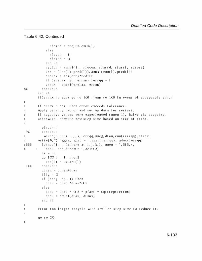
Detailed Code Description
Table 6.42, Continued
rfastd = projtn/cmin(l) else rfasti = 1. rfastd = O. end if redftr = amin1(1., rlocon, rfastd, rfasti, rzrost) err = (cnn(l)-pred(l))/amax1(cnn(l),pred(l)) erelax = abs(err)*redftr if (erelax .gt. errmx) ierrqq = l errmx = amax1(erelax, errmx)8O continue end if if(errmx.lt.eps) go to 1O5 !jump to 1O5 in event of acceptable errorcc If errmx < eps, then error exceeds tolerance. c Apply penalty factor and set up data for restart.c If negative values were experienced (nneg=1), halve the stepsize.c Otherwise, compute new step size based on size of error.c pfact=.4 9O continuec write(6,666) i,j,k,ierrqq,nneg,dtau,cnn(ierrqq),dtremc write(6,*) 'ggen, gdec = ',ggen(ierrqq), gdec(ierrqq)c666 format(1h ,'failure at i,j,k,l, nneg = ',5i5,/,c + 'dtau, cnn,dtrem = ',3e1O.2) ts = tn do 1OO l = 1, ltot2 cnn(l) = cstart(l) 1OO continue dtrem = dtrem+dtau iflg = O if (nneg .eq. 1) then dtau = pfact*dtau*O.5 else dtau = dtau * O.8 * pfact * sqrt(eps/errmx) dtau = amin1(dtau, dtmax) end ifcc Error too large: recycle with smaller step size to reduce it.c
go to 2Oc
6-133
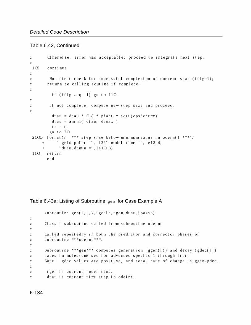
Detailed Code Description
Table 6.42, Continued
c Otherwise, error was acceptable; proceed to integrate next step.c 1O5 continuecc But first check for successful completion of current span (iflg=1);c return to calling routine if complete.c if (iflg .eq. 1) go to 11Occ If not complete, compute new step size and proceed.c dtau = dtau * O.8 * pfact * sqrt(eps/errmx) dtau = amin1( dtau, dtmax ) tn = ts go to 2O 2OOO format(/' *** step size below minimum value in odeint1 ***'/ + ' grid point =', i3/' model time =', e12.4, + 'dtau,dtmin =',2e1O.3) 11O return end
Table 6.43a: Listing of Subroutine gen for Case Example A
subroutine gen(i,j,k,igcalc,tgen,dtau,jpasso)cc Class I subroutine called from subroutine odeintcc Called repeatedly in both the predictor and corrector phases of c subroutine ***odeint***.cc Subroutine ***gen*** computes generation (ggen(l)) and decay (gdec(l)) c rates in moles/cm3 sec for advected species 1 through ltot.c Note: gdec values are positive, and total rate of change is ggen-gdec.cc tgen is current model time.c dtau is current time step in odeint.
6-134

Detailed Code Description
Table 6.43a, Continued
c jpasso is flag specifying predictor (1) or corrector (2,3,...) pass at c current interrogation point in odeint.c
cinclude 'pluvius.com'data xnc /5OO./
cdo l=1,ltot ggen(l)=O. gdec(l)=O.end do
cc define local variablesc
temp=cnn(ltheta)tempc=temp-273.2vsatw=sat(temp)vapor=amin1(cnn(lvapcl),vsatw)cloud=cnn(lvapcl)-vaporjfog(i,j,k)=1if(cloud.le.O.) thenjfog(i,j,k)=Ocloud=O.end ifif (tempc.le.O.) then vsati=ssat(temp) else vsati=vsatwend ifcnn(lwvap)=vaporcnn(lcloud)=cloudrain=cnn(lrain)snow=cnn(lsnow)cnn(lwvap)=vapor
cc Cloud physics block: convert to g/m3 units and initialize rates to O.c
xcloud=cloud*1.8e7xrain=rain*1.8e7xsnow=snow*1.8e7xvapor=vapor*1.8e7
6-135
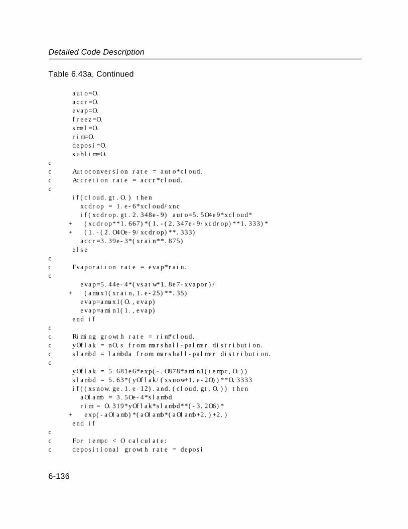
Detailed Code Description
Table 6.43a, Continued
auto=O.accr=O.evap=O.freez=O.smel=O.rim=O.deposi=O.sublim=O.
cc Autoconversion rate = auto*cloud.c Accretion rate = accr*cloud.c
if(cloud.gt.O.) then xcdrop = 1.e-6*xcloud/xnc if(xcdrop.gt.2.348e-9) auto=5.5O4e9*xcloud*
+ (xcdrop**1.667)*(1.-(2.347e-9/xcdrop)**1.333)* + (1.-(2.O4Oe-9/xcdrop)**.333)
accr=3.39e-3*(xrain**.875)else
cc Evaporation rate = evap*rain.c
evap=5.44e-4*(vsatw*1.8e7-xvapor)/ + (amax1(xrain,1.e-25)**.35)
evap=amax1(O.,evap) evap=amin1(1.,evap)end if
cc Riming growth rate = rim*cloud.c yOflak = nO,s from marshall-palmer distribution.c slambd = lambda from marshall-palmer distribution.c
yOflak = 5.681e6*exp(-.O878*amin1(tempc,O.))slambd = 5.63*(yOflak/(xsnow+1.e-2O))**O.3333if((xsnow.ge.1.e-12).and.(cloud.gt.O.)) then aOlamb = 3.5Oe-4*slambd rim = O.319*yOflak*slambd**(-3.2O6)*
+ exp(-aOlamb)*(aOlamb*(aOlamb+2.)+2.)end if
cc For tempc < O calculate:c depositional growth rate = deposi
6-136

Detailed Code Description
Table 6.43a, Continued
c sublimation rate = sublic freezing rate = freez*raincc In calc's for small modisperse ice-crystal case:c ycryst = crystals per cubic meter of spacec xcryst = individual crystal mass (gm)c depcry = depositional growth rate for the crystalsc
if(tempc.lt.O.) then ycryst=amax1(.OO6,4OO.*((-tempc/16.)**4.)) xcryst=amax1(xsnow/ycryst,6.Oe-11) difh2o=.226e-4*((temp/273.15)**1.81)*
+ (1.e6/ptot(i,j,k)) gsi=.82*difh2o*(xvapor-vsati*1.8e7) depcry=ycryst*(.196*xcryst**.38)*gsi*
+ (1.+374.*aflake**.75) if(xsnow.ge.1.e-12) then aOlamb=amax1(O.,alog(yOflak/(slambd*ycryst))) ytflak=(yOflak/slambd)*exp(-aOlamb) aflake=(1.+aOlamb)/slambd deposi=ytflak*(6.28*aflake)*gsi*
+ (1.+374.*aflake**.75) end if deposi=amax1(deposi,depcry)/1.8e7 if(deposi.lt.O.) then sublim=-deposi/snow sublim=amin1(1.,sublim) deposi=O. end if freez = 2.57e-5*ycryst*(xrain*.63) freez = amin1(1.,freez)else
cc For tempc > O calculate:c melting rate = smel*snowc Also, riming rate transfers cloud water to rain category rather than to c snow in this case.c
rmelt=(tempc-4.677e7*(2.693e-7-vapor))* + (7.492e-6*(snow*.667) + 7.415e-4*(snow**.868)) + +1.226e-2*tempc*rim*cloud
smel=rmelt/amax1(snow,1.e-25)
6-137

Detailed Code Description
Table 6.43a, Continued
if(smel.lt.O.) smel=O. smel=amin1(1.O,smel) accr=accr+rim rim=O.end if
cc Calculate ggen and gdec terms for water species.c
ggen(lrain) = (auto+accr)*cloud + smel*snowgdec(lrain) = (evap+freez)*rainggen(lsnow) = deposi + rim*cloud +freez*raingdec(lsnow) = (smel+sublim)*snowggen(lvapcl) = evap*rain + sublim*snowgdec(lvapcl) = (auto+accr+rim)*cloud +deposi
cc Now calculate latent heating terms for theta-c equationc
if(jfog(i,j,k).eq.O) then ggen(ltheta) = (-heatc*evap*rain
+ + (heatc+heatf)*deposi + + heatf*freez*rain)/(cp*cair(i,j,k))
else chi=1.+vapor*heatc*heatc/(cp*glc*temp*temp*cair(i,j,k)) ggen(ltheta) = heatf*(deposi+freez*rain)/(chi*cp*cair(i,j,k))end ifreturnend
Table 6.43b: Listing of Subroutine gen for Case Example B
subroutine gen(i,j,k,tgen,dtau,jpasso)cc Class I subroutine called from subroutine odeintcc Called repeatedly in both the predictor and corrector phases of c subroutine ***odeint***.
6-138

Detailed Code Description
Table 6.43b, Continued
cc Subroutine ***gen*** computes generation (ggen(l)) and decay gdec((l)) c rates in moles/cm3 sec for advected species 1 through ltot.cc Note: gdec values are positive, and total rate of change is ggen-gdec.c c tgen is current model time.c dtau is current time step in odeint.c jpassO is flag specifying predictor (1) or corrector (2,3,...).c pass at current interrogation point in odeint.c include 'pluvius.com' data xnc /5OO./ data ijkold /O/ ijknew = i+j+k if(ijknew.eq.ijkold) go to 1OO ijkold=ijknewc do l=1,ltot ggen(l)=O. gdec(l)=O. end docc Define local variables.c temp=cnn(ltemp) tempc=temp-273.2 vsatw=sat(temp) vapor=amin1(cnn(lvapcl),vsatw) if (tempc.le.O.) then vsati=ssat(temp) else vsati=vsatw end if rain=cnn(lrain) snow=cnn(lsnow) cloud=cnn(lcloud)cc Cloud physics block: convert to g/m3 and initialize rates.c xcloud=cloud*1.8e7 xrain=rain*1.8e7
6-139

Detailed Code Description
Table 6.43b, Continued
xsnow=snow*1.8e7 xvapor=vapor*1.8e7 auto=O. accr=O. evap=O. freez=O. smel=O. rim=O. deposi=O. sublim=O.cc Autoconversion rate = auto*cloud.c Accretion rate = accr*cloud.c if(cloud.gt.O.) then xcdrop = 1.e-6*xcloud/xnc if(xcdrop.gt.2.348e-9) auto=5.5O4e9*xcloud* + (xcdrop**1.667)*(1.-(2.347e-9/xcdrop)**1.333)* + (1.-(2.O4Oe-9/xcdrop)**.333) accr=3.39e-3*(xrain**.875) elsecc Evaporation rate = evap*rain.c evap=5.44e-4*(vsatw*1.8e7-xvapor)/ + (amax1(xrain,1.e-25)**.35) evap=amax1(O.,evap) evap=amin1(1.,evap) end ifcc Riming growth rate = rim*cloud.c yOflak = nO,s from marshall-palmer distribution.c slambd = lambda from marshall-palmer distribution.c yOflak = 5.681e6*exp(-.O878*amin1(tempc,O.)) slambd = 5.63*(yOflak/(xsnow+1.e-2O))**O.3333 if((xsnow.ge.1.e-12).and.(cloud.gt.O.)) then aOlamb = 3.5Oe-4*slambd rim = O.319*yOflak*(slambd**(-3.2O6))*exp(-aOlamb)* + (aOlamb*(aOlamb+2.)+2.) end if
6-140

Detailed Code Description
Table 6.43b, Continued
c For tempc < O calculate:c depositional growth rate = deposic sublimation rate = sublic freezing rate = freez*raincc In calc's for small modisperse ice-crystal case:c ycryst = crystals per cubic meter of spacec xcryst = individual crystal mass (gm)c depcry = depositional growth rate for the crystalsc if(tempc.lt.O.) then ycryst=amax1(.OO6,4OO.*((-tempc/16.)**4.)) xcryst=amax1(xsnow/ycryst,6.Oe-11) difh2o=.226e-4*((temp/273.15)**1.81)* + (1.e6/ptot(i,j,k)) gsi=.82*difh2o*(xvapor-vsati*1.8e7) depcry=ycryst*(.196*xcryst**.38)*gsi* + (1.+374.*aflake**.75) if(xsnow.ge.1.e-12) then aOlamb=amax1(O.,alog(yOflak/(slambd*ycryst))) ytflak=(yOflak/slambd)*exp(-aOlamb) aflake=(1.+aOlamb)/slambd deposi=ytflak*(6.28*aflake)*gsi* + (1.+374.*aflake**.75) end if deposi=amax1(deposi,depcry)/1.8e7 if(deposi.lt.O.) then sublim=-deposi/snow sublim=amin1(1.,sublim) deposi=O. end if freez = 2.57e-5*ycryst*(xrain*.63) freez = amin1(1.,freez) elsecc For tempc > O calculate:c melting rate = smel*snowc Also, riming rate transfers cloud water to rain category rather than c to snow in this case.c rmelt=(tempc-4.677e7*(2.693e-7-vapor))*
6-141
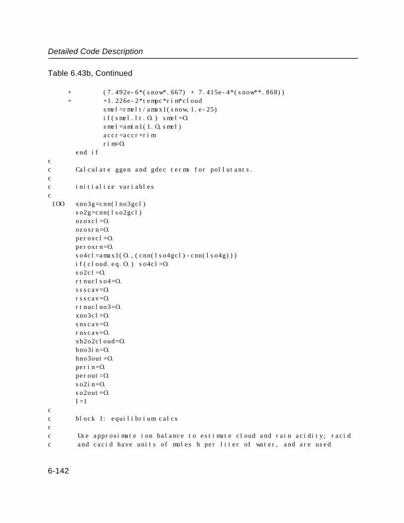
Detailed Code Description
Table 6.43b, Continued
+ (7.492e-6*(snow*.667) + 7.415e-4*(snow**.868)) + +1.226e-2*tempc*rim*cloud smel=rmelt/amax1(snow,1.e-25) if(smel.lt.O.) smel=O. smel=amin1(1.O,smel) accr=accr+rim rim=O. end ifcc Calculate ggen and gdec terms for pollutants.cc initialize variablesc 1OO xno3g=cnn(lno3gcl) so2g=cnn(lso2gcl) ozoxcl=O. ozoxrn=O. peroxcl=O. peroxrn=O. so4cl=amax1(O.,(cnn(lso4gcl)-cnn(lso4g))) if(cloud.eq.O.) so4cl=O. so2cl=O. rtnuclso4=O. ssscav=O. rsscav=O. rtnuclno3=O. xno3cl=O. snscav=O. rnscav=O. xh2o2cloud=O. hno3in=O. hno3out=O. perin=O. perout=O. so2in=O. so2out=O. I=1cc block 1: equilibrium calcscc Use approximate ion balance to estimate cloud and rain acidity; racid c and cacid have units of moles h per liter of water, and are used
6-142
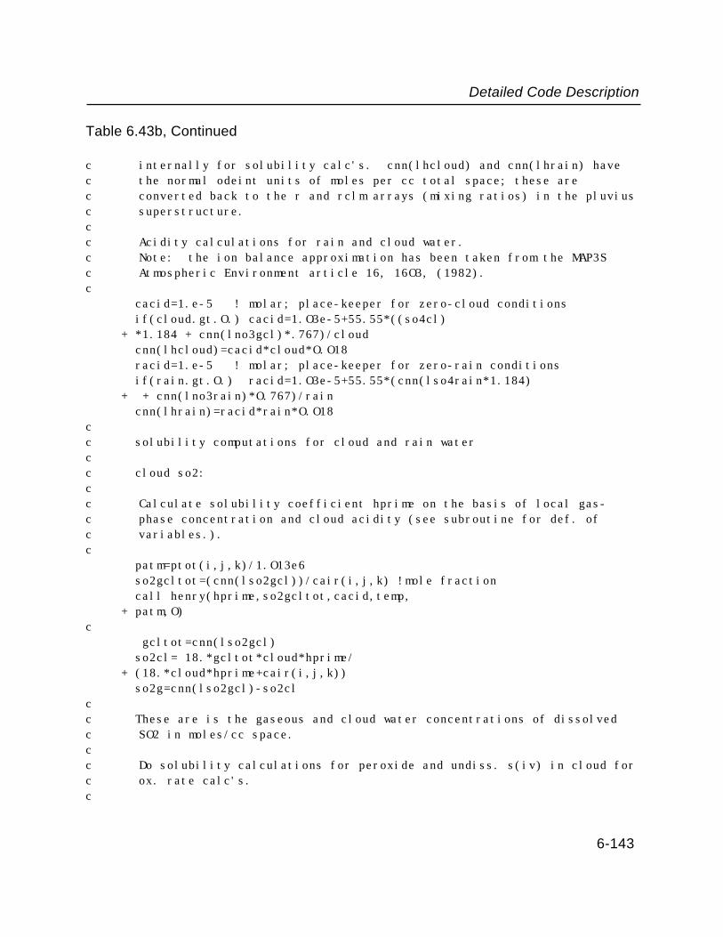
Detailed Code Description
Table 6.43b, Continued
c internally for solubility calc's. cnn(lhcloud) and cnn(lhrain) have c the normal odeint units of moles per cc total space; these are c converted back to the r and rclm arrays (mixing ratios) in the pluviusc superstructure.cc Acidity calculations for rain and cloud water.c Note: the ion balance approximation has been taken from the MAP3Sc Atmospheric Environment article 16, 16O3, (1982).c cacid=1.e-5 ! molar; place-keeper for zero-cloud conditions if(cloud.gt.O.) cacid=1.O3e-5+55.55*((so4cl) + *1.184 + cnn(lno3gcl)*.767)/cloud cnn(lhcloud)=cacid*cloud*O.O18 racid=1.e-5 ! molar; place-keeper for zero-rain conditions if(rain.gt.O.) racid=1.O3e-5+55.55*(cnn(lso4rain*1.184) + + cnn(lno3rain)*O.767)/rain cnn(lhrain)=racid*rain*O.O18cc solubility computations for cloud and rain watercc cloud so2:cc Calculate solubility coefficient hprime on the basis of local gas-c phase concentration and cloud acidity (see subroutine for def. of c variables.).c patm=ptot(i,j,k)/1.O13e6 so2gcltot=(cnn(lso2gcl))/cair(i,j,k) !mole fraction call henry(hprime,so2gcltot,cacid,temp, + patm,O)c gcltot=cnn(lso2gcl) so2cl= 18.*gcltot*cloud*hprime/ + (18.*cloud*hprime+cair(i,j,k)) so2g=cnn(lso2gcl)-so2clcc These are is the gaseous and cloud water concentrations of dissolved c SO2 in moles/cc space.cc Do solubility calculations for peroxide and undiss. s(iv) in cloud for c ox. rate calc's.c
6-143

Detailed Code Description
Table 6.43b, Continued
solh=8.2414e-6*exp(6834.93/temp) !moles/liter-atmosphere sols=exp(-1O.21+3112./temp) !moles/liter atmosphere patmcs=patm/cair(i,j,k) solh=solh*patmcs*.OO1 !dimensionless units aqh=1OOO.*solh*cnn(lh2o2gcl)/(1.+18.*solh*cloud) aqs=sols*(so2g)*patmcs xh2o2cloud=aqh*.O18*cloud ! distributed cloudwater peroxide conc.cc aqh and aqs are, respectively, the molar concentrations ofc peroxide and undissociated s(iv) (moles/liter cloud water).cc Compute distributed solubility parameter for rainborne h2o2 (for c mass-transfer calc's below).c if(rain.gt.O.) then xip=18.*solh*raincc Compute disperse-phase SO2 solubility parameter for rain (to be used c below for mass-transfer calc's).c crainso2=(cnn(lso2rain))/(18.*rain) call henry(hprime,crainso2,racid,temp,patm,1) rso2eq=crainso2*hprime cso2eq=rso2eq*cair(i,j,k) xis=cnn(lso2rain)/cso2eq end ifcc Nitric acid solubility calculations:cc Compute distributed HNO3 solubility in cloud water:c if (cnn(lhcloud).gt.O.) then xin=4.96e-6*cloud*cloud*exp(87O6./temp)/cnn(lhcloud) xno3cl=xin*cnn(lno3gcl)/(1.+xin) hno3g=cnn(lno3gcl)-xno3cl else xno3cl=O. hno3g=cnn(lno3gcl) end ifcc This is the cloud water concentration of nitrate ion in moles/cc c space. c
6-144
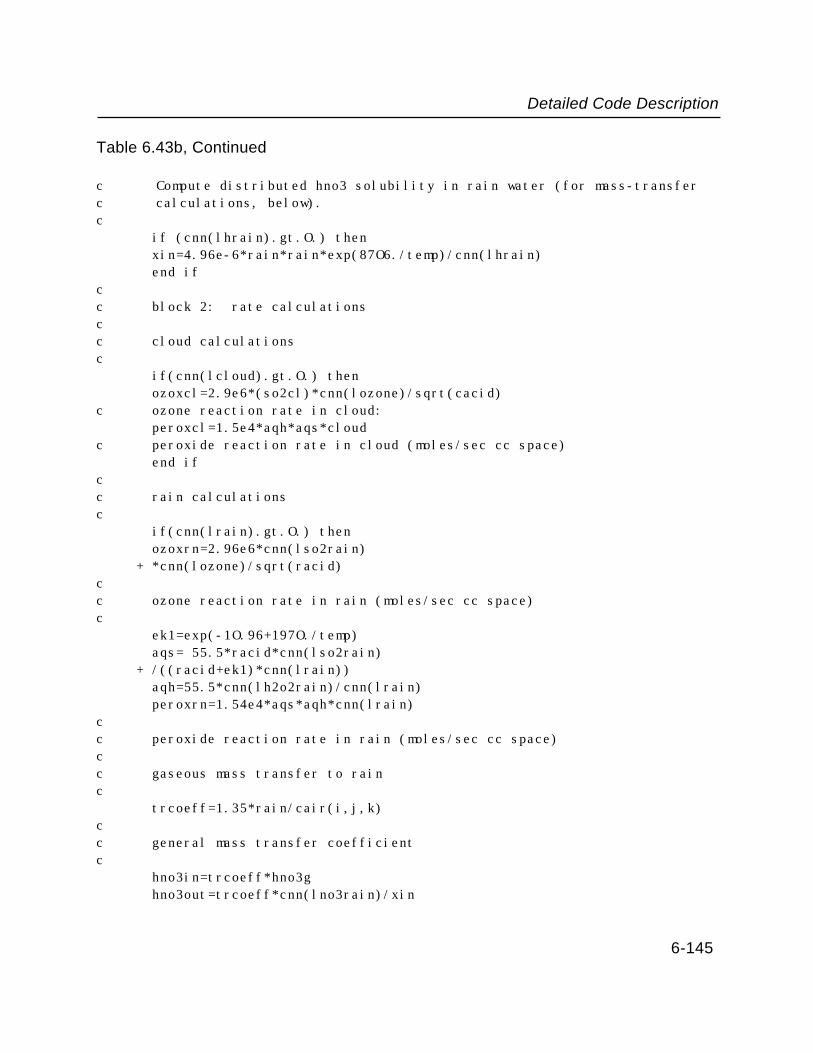
Detailed Code Description
Table 6.43b, Continued
c Compute distributed hno3 solubility in rain water (for mass-transferc calculations, below).c if (cnn(lhrain).gt.O.) then xin=4.96e-6*rain*rain*exp(87O6./temp)/cnn(lhrain) end ifcc block 2: rate calculationscc cloud calculationsc if(cnn(lcloud).gt.O.) then ozoxcl=2.9e6*(so2cl)*cnn(lozone)/sqrt(cacid)c ozone reaction rate in cloud: peroxcl=1.5e4*aqh*aqs*cloudc peroxide reaction rate in cloud (moles/sec cc space) end ifcc rain calculationsc if(cnn(lrain).gt.O.) then ozoxrn=2.96e6*cnn(lso2rain) + *cnn(lozone)/sqrt(racid)cc ozone reaction rate in rain (moles/sec cc space)c ek1=exp(-1O.96+197O./temp) aqs= 55.5*racid*cnn(lso2rain) + /((racid+ek1)*cnn(lrain)) aqh=55.5*cnn(lh2o2rain)/cnn(lrain) peroxrn=1.54e4*aqs*aqh*cnn(lrain)cc peroxide reaction rate in rain (moles/sec cc space)cc gaseous mass transfer to rainc trcoeff=1.35*rain/cair(i,j,k)cc general mass transfer coefficientc hno3in=trcoeff*hno3g hno3out=trcoeff*cnn(lno3rain)/xin
6-145
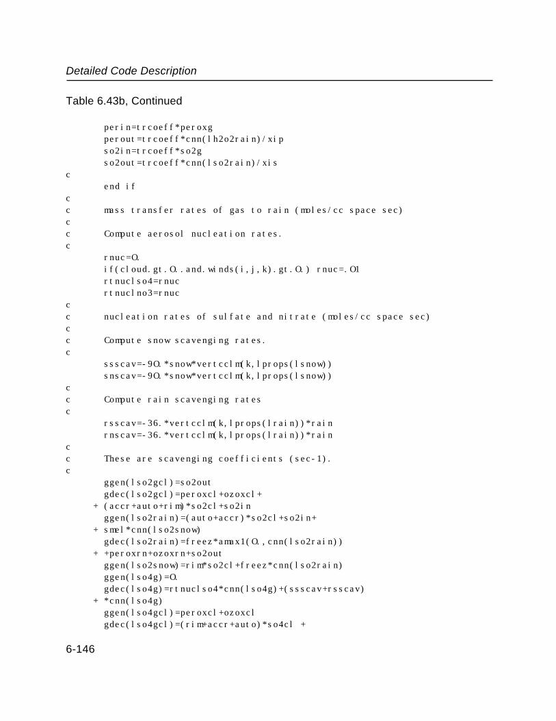
Detailed Code Description
Table 6.43b, Continued
perin=trcoeff*peroxg perout=trcoeff*cnn(lh2o2rain)/xip so2in=trcoeff*so2g so2out=trcoeff*cnn(lso2rain)/xisc end ifcc mass transfer rates of gas to rain (moles/cc space sec)cc Compute aerosol nucleation rates.c rnuc=O. if(cloud.gt.O..and.winds(i,j,k).gt.O.) rnuc=.O1 rtnuclso4=rnuc rtnuclno3=rnuccc nucleation rates of sulfate and nitrate (moles/cc space sec)cc Compute snow scavenging rates.c ssscav=-9O.*snow*vertcclm(k,lprops(lsnow)) snscav=-9O.*snow*vertcclm(k,lprops(lsnow))cc Compute rain scavenging ratesc rsscav=-36.*vertcclm(k,lprops(lrain))*rain rnscav=-36.*vertcclm(k,lprops(lrain))*raincc These are scavenging coefficients (sec-1).c ggen(lso2gcl)=so2out gdec(lso2gcl)=peroxcl+ozoxcl+ + (accr+auto+rim)*so2cl+so2in ggen(lso2rain)=(auto+accr)*so2cl+so2in+ + smel*cnn(lso2snow) gdec(lso2rain)=freez*amax1(O.,cnn(lso2rain)) + +peroxrn+ozoxrn+so2out ggen(lso2snow)=rim*so2cl+freez*cnn(lso2rain) ggen(lso4g)=O. gdec(lso4g)=rtnuclso4*cnn(lso4g)+(ssscav+rsscav) + *cnn(lso4g) ggen(lso4gcl)=peroxcl+ozoxcl gdec(lso4gcl)=(rim+accr+auto)*so4cl +
6-146

Detailed Code Description
Table 6.43b, Continued
+ (ssscav+rsscav)*cnn(lso4g) ggen(lso4rain)=peroxrn+ozoxrn+rsscav*cnn(lso4g)+ + smel*cnn(lso4snow)+(auto+accr)*so4cl gdec(lso4rain)=freez*cnn(lso4rain) ggen(lso4snow)=ssscav*cnn(lso4g)+freez*cnn(lso4rain)+ + rim*so4cl gdec(lso4snow)=smel*cnn(lso4snow) ggen(lno3gcl)=rtnuclno3*cnn(lno3g)+hno3out gdec(lno3gcl)=(rim+accr+auto)*xno3cl+hno3in ggen(lno3g)=O. gdec(lno3g)=(snscav+rnscav)*cnn(lno3g)+ + rtnuclno3*cnn(lno3g) ggen(lno3rain)=(auto+accr)*xno3cl+rnscav*cnn(lno3g)+ + smelt*cnn(lno3snow)+hno3in gdec(lno3rain)=freez*cnn(lno3rain)+hno3out ggen(lno3snow)=snscav*cnn(lno3g)+freez*cnn(lno3rain) gdec(lno3snow)=smel*cnn(lno3snow) ggen(lh2o2gcl)=perout gdec(lh2o2gcl)=(auto+accr+rim)*xh2o2cloud+peroxcl+ + perin ggen(lh2o2rain)=(auto+accr)*xh2o2cloud+perin+ + smel*cnn(lh2o2snow) gdec(lh2o2rain)=peroxrn+freez*cnn(lh2o2rain)+perout ggen(lh2o2snow)=rim*xh2o2cloud+freez*cnn(lh2o2rain) gdec(lh2o2snow)=smel*cnn(lh2o2snow) ggen(lozone)=O. gdec(lozone)=ozoxcl+ozoxrn ijkold=ijknew return end
6-147
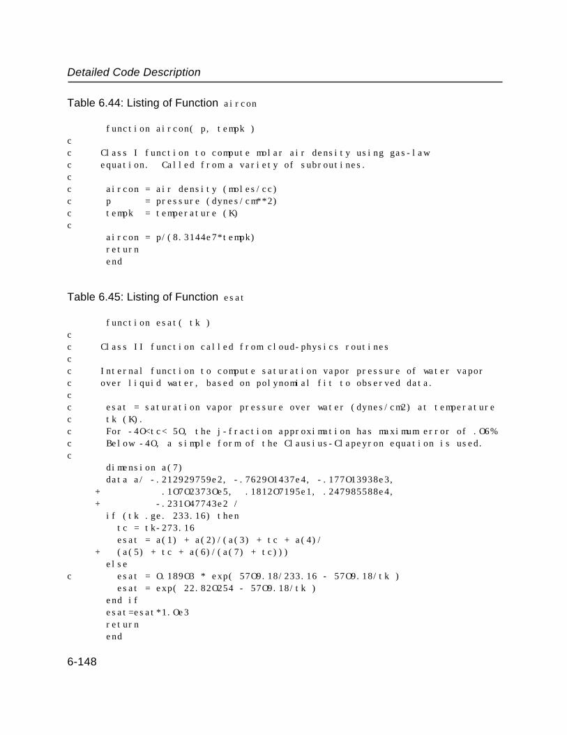
Detailed Code Description
Table 6.44: Listing of Function aircon
function aircon( p, tempk )cc Class I function to compute molar air density using gas-law c equation. Called from a variety of subroutines.cc aircon = air density (moles/cc)c p = pressure (dynes/cm**2)c tempk = temperature (K)c aircon = p/(8.3144e7*tempk) return end
Table 6.45: Listing of Function esat
function esat( tk )cc Class II function called from cloud-physics routinescc Internal function to compute saturation vapor pressure of water vapor c over liquid water, based on polynomial fit to observed data.cc esat = saturation vapor pressure over water (dynes/cm2) at temperaturec tk (K).c For -4O<tc< 5O, the j-fraction approximation has maximum error of .O6%c Below -4O, a simple form of the Clausius-Clapeyron equation is used.c dimension a(7) data a/ -.212929759e2, -.7629O1437e4, -.177O13938e3, + .1O7O2373Oe5, .1812O7195e1, .247985588e4, + -.231O47743e2 / if (tk .ge. 233.16) then tc = tk-273.16 esat = a(1) + a(2)/(a(3) + tc + a(4)/ + (a(5) + tc + a(6)/(a(7) + tc))) elsec esat = O.189O3 * exp( 57O9.18/233.16 - 57O9.18/tk ) esat = exp( 22.82O254 - 57O9.18/tk ) end if esat=esat*1.Oe3 return end
6-148

Detailed Code Description
Table 6.46: Listing of Function esati
function esati( tk )cc Class II function called from cloud-physics routinescc Computes saturation vapor pressure of water vapor over ice, based on fit c to observed data.cc esati = saturation vapor pressure over ice (dynes/cm2) at temperaturec tk (K).c For -5O< tc<5O, the j-fraction approximation has maximum error of .O2%c Below -5O, a simple form of the Clausius-Clapeyron equation is used.c dimension a(7) data a/ -.136O7654Oe1, -.34O752185e3, -.97O586O93e2, + .532O49788e4, .268793249e2, .113134694e4, + .147762227e2 / if (tk .ge. 223.16) then tc = tk-273.16 esati = a(1) + a(2)/(a(3) + tc + a(4)/ + (a(5) + tc + a(6)/(a(7) + tc))) elsec esati = O.O39343 * exp( 615O.O9/223.16 - 615O.O9/tk ) esati = exp( 24.32367 - 615O.O9/tk ) end if esati=esati*1.Oe3 return end
Table 6.47: Listing of Function sat
function sat (tk)cc Class II function called from a variety of subroutines:c Computes concentration of saturated water vapor overc liquid water, using gas-law equation.c sat = saturation vapor concentration (moles h2o/cm**3) over water at c temperature tk (K).c sat = esat(tk) / (8.3144e7 * tk) return end
6-149

Detailed Code Description
Table 6.48: Listing of Function ssat
function ssat (tk)cc Class II function called from a variety of subroutines.c Function to compute equilibrium concentration of water vapor c over ice, using gas-law equation.c ssat = saturation vapor concentration (moles h2o/cm**3)c over ice at temperature tk (K).c ssat = esati(tk)/ (8.3144e7 * tk) return end
Table 6.49: Listing of Function rlapse
function rlapse ( tempk, cair,jfog )cc Class II function called from subroutine init.c Calculates the adiabatic lapse rate under wet or dryc conditions, based on hydrostatic equation.cc rlapse = lapse rate (deg. K/cm)c adiabatic if jfog=Oc pseudoadiabatic otherwisec tempk = temperature (K)c cair = air density (moles/cc)cc Thermodynamic units are cgs (constants use moles).c The sat function must return the saturation vapor density (moles/cc) at c temperature tempk.c data gammad/-9.76e-5/! dry adiabatic lapse rate (deg k/cm) data cp/2.91e8/ ! air heat capacity, constant pressure (erg/mole/deg k) data r/8.314e7/ ! gas constatn (erg/mole/deg k) data hlc/4.5e11/ ! latent heat of condensation (erg/mole water) rlapse = gammad if (jfog.ne.O) then dummy1 = hlc*sat(tempk)/(cair*r*tempk) rlapse = gammad*(1. + dummy1)/(1. + dummy1*hlc/(cp*tempk)) end if return end
6-150

Detailed Code Description
Table 6.50: Listing of Subroutine henry
subroutine henry ( hprime, conc, hex, t, p, lgopt )cc Class III subroutine called from subroutine gencc Subroutine for calculating apparent henry's-law constant on the basis ofc Johnstone-Leppla parameters, using the equations of Hales and Sutter.cc hprime is the apparent henry's-law constant, defined by:c hprime = so2_gas / so2_aq, where:c so2_aq = concentration of sulfur-IV in aqueous phase c (moles/cm**3 water)c so2_gas = concentration of gas phase so2 (mole fraction)c c is eitherc so2_aq when lgopt = 1 (moles/cm**3 water)c so2_gas when lgopt = O (mole fraction)c hex is the aqueous phase hydrogen ion concentration from speciesc other than sulfur-IV (molar)c t is temperature (degrees k)c p is atmospheric pressure (atmospheres)c lgopt is a flag explained abovec if ((lgopt.ne.O) .and. (lgopt.ne.1)) then
write(*,*) 'Bad lgopt in subroutine henry' stop end if
hank = exp(1O.21-3112./t)/p eqcon = exp(-1O.96+197O./t) b=eqcon+hex if(lgopt.ne.1) go to 2Occ lgopt=1 --> conc is the aqueous concentrationc cdum=eqcon*1OOO.*conc test1=4.*cdum/(b*b) if(test1.gt..OO1) go to 1O hprime=hank*(1.-eqcon/b) go to 4O 1O hprime = hank*(1.+(b-sqrt(b*b+4.*cdum))/(2OOO.*conc)) go to 4Occ lgopt=O --> conc is the gas phase concentrationc
6-151

Detailed Code Description
Table 6.50, Continued
2O test1 = 4.*eqcon*conc/(hex*hex*hank) if(test1 .gt. .OO1) go to 3O hprime=hank*hex/b go to 4O 3O hprime=conc/(conc/hank- + (hex-sqrt(hex*hex+4.*conc*eqcon/hank))/2.) 4O hprime = hprime*1OOO. return end
Table 6.51: Listing of Subroutine tfrmth
subroutine tfrmth(p,th,rvc,jfog,t)cc Class II subroutine called from subroutines cleanup and chmint.cc Converts equivalent potential temperature to absolute temperature,c based on equations (2.7) and (2.8). Since absolute temperature isc an implicit variable in these equations, this subroutine is basedc on a two-dimensional interpolation of tabulated solutions toc these equations; i.e. T = T(tbase, pbase), where c tbase = base values of potential temperature function:c th*(p/1OOOOOO.)**xk+alpha*rvcc pbase = base values of pressurec base = array of tabulated absolute temperaturescc in subroutine argument list:cc p pressure, dynes/cm2c th equivalent potential temperature in degrees kelvinc rvc mixing ratio of vapor + cloud waterc jfog flag indicating saturation conditions: c 1 if saturated; O otherwise
6-152

Detailed Code Description
Table 6.51, Continued
c t temperature in degrees kelvinc dimension pbase(11),tbase(36),base(11,36) data alpha/1725./ data xk/O.286/ data (tbase(i),i=1,36)/ + O.23OOOOOe+O3, O.235OOOOe+O3, O.24OOOOOe+O3, O.245OOOOe+O3, + O.25OOOOOe+O3, O.255OOOOe+O3, O.26OOOOOe+O3, O.265OOOOe+O3, + O.27OOOOOe+O3, O.275OOOOe+O3, O.28OOOOOe+O3, O.285OOOOe+O3, + O.29OOOOOe+O3, O.295OOOOe+O3, O.3OOOOOOe+O3, O.3O5OOOOe+O3, + O.31OOOOOe+O3, O.315OOOOe+O3, O.32OOOOOe+O3, O.325OOOOe+O3, + O.33OOOOOe+O3, O.335OOOOe+O3, O.34OOOOOe+O3, O.345OOOOe+O3, + O.35OOOOOe+O3, O.355OOOOe+O3, O.36OOOOOe+O3, O.365OOOOe+O3, + O.37OOOOOe+O3, O.375OOOOe+O3, O.38OOOOOe+O3, O.385OOOOe+O3, + O.39OOOOOe+O3, O.395OOOOe+O3, O.4OOOOOOe+O3, O.4O5OOOOe+O3/ data (pbase(i), i=1,11)/ + O.1OOOOe+O6, O.2OOOOe+O6, O.3OOOOe+O6, O.4OOOOe+O6, + O.5OOOOe+O6, O.6OOOOe+O6, O.7OOOOe+O6, O.8OOOOe+O6, + O.9OOOOe+O6, O.1OOOOe+O7, O.11OOOe+O7/ data (base(1,i), i=1,36)/ + O.2281O5Oe+O3, O.232O88Oe+O3, O.2357452e+O3, O.239O75Oe+O3, + O.242O81Oe+O3, O.244786Oe+O3, O.247221Oe+O3, O.24942OOe+O3, + O.251414Oe+O3, O.2532313e+O3, O.2548961e+O3, O.256429Oe+O3, + O.257847Oe+O3, O.259165Oe+O3, O.26O3941e+O3, O.261546Oe+O3, + O.262629Oe+O3, O.26365OOe+O3, O.2646152e+O3, O.2655312e+O3, + O.2664O2Oe+O3, O.267232Oe+O3, O.268O25Oe+O3, O.268783Oe+O3, + O.26951OOe+O3, O.27O2O8Oe+O3, O.27O8791e+O3, O.271526Oe+O3, + O.2721493e+O3, O.272752Oe+O3, O.273334Oe+O3, O.2738973e+O3, + O.2744431e+O3, O.274973Oe+O3, O.275487Oe+O3, O.2759864e+O3/ data (base(2,i), i=1,36)/ + O.22896OOe+O3, O.233339Oe+O3, O.237471Oe+O3, O.2413184e+O3, + O.2448583e+O3, O.248O88Oe+O3, O.251O22Oe+O3, O.253684Oe+O3, + O.2561O2Oe+O3, O.2583O43e+O3, O.26O3182e+O3, O.2621671e+O3, + O.263872Oe+O3, O.265451Oe+O3, O.2669181e+O3, O.268288Oe+O3, + O.269571Oe+O3, O.27O777Oe+O3, O.2719134e+O3, O.2729882e+O3, + O.274OO7Oe+O3, O.2749754e+O3, O.275898Oe+O3, O.2767782e+O3, + O.27762O3e+O3, O.2784273e+O3, O.2792O2Oe+O3, O.2799461e+O3, + O.28O663Oe+O3, O.281354Oe+O3, O.282O211e+O3, O.282666Oe+O3, + O.2832894e+O3, O.283894Oe+O3, O.28448OOe+O3, O.285O483e+O3/ data (base(3,i), i=1,36)/ + O.229282Oe+O3, O.233834Oe+O3, O.2381894e+O3, O.2423O4Oe+O3, + O.246141Oe+O3, O.2496832e+O3, O.25293O1e+O3, O.255895Oe+O3,
6-153

Detailed Code Description
Table 6.51, Continued
+ O.258598Oe+O3, O.261O644e+O3, O.263321Oe+O3, O.265391Oe+O3, + O.267298Oe+O3, O.269O6OOe+O3, O.27O6951e+O3, O.2722183e+O3, + O.273642Oe+O3, O.274978Oe+O3, O.2762341e+O3, O.27742OOe+O3, + O.2785421e+O3, O.2796O7Oe+O3, O.28O6193e+O3, O.281585Oe+O3, + O.2825O62e+O3, O.2833883e+O3, O.284234Oe+O3, O.285O46Oe+O3, + O.285827Oe+O3, O.286579Oe+O3, O.2873O41e+O3, O.288OO5Oe+O3, + O.288682Oe+O3, O.2893372e+O3, O.2899722e+O3, O.29O5883e+O3/ data (base(4,i), i=1,36)/ + O.2294512e+O3, O.2341O1Oe+O3, O.238588Oe+O3, O.242867Oe+O3, + O.246898Oe+O3, O.25O654Oe+O3, O.254124Oe+O3, O.2573111e+O3, + O.26O23OOe+O3, O.2629OOOe+O3, O.2653453e+O3, O.26759OOe+O3, + O.2696561e+O3, O.271565Oe+O3, O.273334Oe+O3, O.2749794e+O3, + O.276516Oe+O3, O.277955Oe+O3, O.2793O7Oe+O3, O.28O5811e+O3, + O.281786Oe+O3, O.282927Oe+O3, O.284O111e+O3, O.285O44Oe+O3, + O.286O29Oe+O3, O.28697O3e+O3, O.2878724e+O3, O.288738Oe+O3, + O.28957OOe+O3, O.29O37OOe+O3, O.291142Oe+O3, O.2918861e+O3, + O.2926O6Oe+O3, O.2933O2Oe+O3, O.293976Oe+O3, O.2946292e+O3/ data (base(5,i), i=1,36)/ + O.229556Oe+O3, O.2342682e+O3, O.238842Oe+O3, O.2432334e+O3, + O.2474O2Oe+O3, O.251315Oe+O3, O.2549543e+O3, O.258316Oe+O3, + O.2614O6Oe+O3, O.264242Oe+O3, O.2668431e+O3, O.269233Oe+O3, + O.271433Oe+O3, O.2734642e+O3, O.2753461e+O3, O.277O953e+O3, + O.278727Oe+O3, O.28O2534e+O3, O.281687Oe+O3, O.283O36Oe+O3, + O.28431OOe+O3, O.2855162e+O3, O.2866613e+O3, O.287751Oe+O3, + O.2887891e+O3, O.2897813e+O3, O.29O731Oe+O3, O.291642Oe+O3, + O.2925164e+O3, O.293358Oe+O3, O.2941684e+O3, O.29495O3e+O3, + O.2957O6Oe+O3, O.296436Oe+O3, O.297143Oe+O3, O.297828Oe+O3/ data (base(6,i), i=1,36)/ + O.2296271e+O3, O.234383Oe+O3, O.239O18Oe+O3, O.243492Oe+O3, + O.247763Oe+O3, O.251797Oe+O3, O.25557O1e+O3, O.259O723e+O3, + O.2623O51e+O3, O.26528OOe+O3, O.268O14Oe+O3, O.27O528Oe+O3, + O.272844Oe+O3, O.2749822e+O3, O.276963Oe+O3, O.2788O22e+O3, + O.28O517Oe+O3, O.28212O4e+O3, O.2836244e+O3, O.285O4OOe+O3, + O.286375Oe+O3, O.287638Oe+O3, O.2888363e+O3, O.289976Oe+O3, + O.291O61Oe+O3, O.292O98Oe+O3, O.293O891e+O3, O.294O4OOe+O3, + O.294952Oe+O3, O.2958291e+O3, O.296674Oe+O3, O.297489Oe+O3, + O.298275Oe+O3, O.299O352e+O3, O.299771Oe+O3, O.3OO484Oe+O3/ data (base(7,i), i=1,36)/ + O.229679Oe+O3, O.234467Oe+O3, O.2391474e+O3, O.243684Oe+O3, + O.248O35Oe+O3, O.252165Oe+O3, O.256O471e+O3, O.259667Oe+O3, + O.263O2OOe+O3, O.266114Oe+O3, O.2689631e+O3, O.271587Oe+O3, + O.274OO5Oe+O3, O.276238Oe+O3, O.2783O6Oe+O3, O.28O227Oe+O3, + O.282O16Oe+O3, O.2836881e+O3, O.285256Oe+O3, O.28673OOe+O3,
6-154
Detailed Code Description
Table 6.51, Continued
+ O.28812OOe+O3, O.2894344e+O3, O.29O68O4e+O3, O.2918644e+O3, + O.2929921e+O3, O.294O683e+O3, O.295O98Oe+O3, O.296O834e+O3, + O.297O3OOe+O3, O.297939Oe+O3, O.298815Oe+O3, O.2996583e+O3, + O.3OO473Oe+O3, O.3O126OOe+O3, O.3O2O22Oe+O3, O.3O276OOe+O3/ data (base(8,i), i=1,36)/ + O.229718Oe+O3, O.23453O1e+O3, O.239247Oe+O3, O.243832Oe+O3, + O.248247Oe+O3, O.252456Oe+O3, O.256429Oe+O3, O.26O1472e+O3, + O.2636O41e+O3, O.2668O24e+O3, O.269754Oe+O3, O.272475Oe+O3, + O.2749843e+O3, O.2773O31e+O3, O.27945O4e+O3, O.2814443e+O3, + O.2833O14e+O3, O.285O362e+O3, O.286662Oe+O3, O.28819OOe+O3, + O.28963OOe+O3, O.29O991Oe+O3, O.292281Oe+O3, O.2935O54e+O3, + O.294672Oe+O3, O.2957841e+O3, O.296848Oe+O3, O.297866Oe+O3, + O.298843Oe+O3, O.299782Oe+O3, O.3OO6851e+O3, O.3O1556Oe+O3, + O.3O2396Oe+O3, O.3O32O74e+O3, O.3O3993Oe+O3, O.3O4753Oe+O3/ data (base(9,i), i=1,36)/ + O.2297481e+O3, O.23458O2e+O3, O.2393253e+O3, O.24395O2e+O3, + O.248418Oe+O3, O.252692Oe+O3, O.2567413e+O3, O.26O5452e+O3, + O.264O93Oe+O3, O.267383Oe+O3, O.27O4252e+O3, O.273234Oe+O3, + O.275827Oe+O3, O.278224Oe+O3, O.28O4434e+O3, O.2825O5Oe+O3, + O.284424Oe+O3, O.2862164e+O3, O.2878954e+O3, O.289473Oe+O3, + O.29O9591e+O3, O.2923632e+O3, O.2936931e+O3, O.294956Oe+O3, + O.2961574e+O3, O.2973O34e+O3, O.2983984e+O3, O.299447Oe+O3, + O.3OO4522e+O3, O.3O1418Oe+O3, O.3O23472e+O3, O.3O3243Oe+O3, + O.3O41O61e+O3, O.3O494O3e+O3, O.3O57471e+O3, O.3O6528Oe+O3/ data (base(1O,i), i=1,36)/ + O.229773Oe+O3, O.234621Oe+O3, O.239389Oe+O3, O.244O47Oe+O3, + O.248558Oe+O3, O.252887Oe+O3, O.257OO3Oe+O3, O.26O881Oe+O3, + O.2645O8Oe+O3, O.267881Oe+O3, O.271OO5Oe+O3, O.2738931e+O3, + O.2765621e+O3, O.279O31Oe+O3, O.2813174e+O3, O.283441Oe+O3, + O.285418Oe+O3, O.287264Oe+O3, O.288993Oe+O3, O.29O6162e+O3, + O.2921454e+O3, O.29359OOe+O3, O.294957Oe+O3, O.296255Oe+O3, + O.29749OOe+O3, O.298667Oe+O3, O.2997912e+O3, O.3OO868Oe+O3, + O.3O19OOOe+O3, O.3O289O4e+O3, O.3O3844Oe+O3, O.3O4762Oe+O3, + O.3O56473e+O3, O.3O65O24e+O3, O.3O73293e+O3, O.3O813OOe+O3/ data (base(11,i), i=1,36)/ + O.229793Oe+O3, O.234654Oe+O3, O.239442Oe+O3, O.244127Oe+O3, + O.248675Oe+O3, O.253O52Oe+O3, O.2572242e+O3, O.261168Oe+O3, + O.264866Oe+O3, O.268313Oe+O3, O.2715114e+O3, O.274473Oe+O3, + O.277212Oe+O3, O.279747Oe+O3, O.282O96Oe+O3, O.2842771e+O3, + O.2863O8Oe+O3, O.2882O41e+O3, O.2899793e+O3, O.2916462e+O3, + O.293216Oe+O3, O.2946974e+O3, O.2961OOOe+O3, O.297431Oe+O3, + O.298697Oe+O3, O.2999O31e+O3, O.3O1O552e+O3, O.3O2158Oe+O3,
6-155

Detailed Code Description
Table 6.51, Continued
+ O.3O3215Oe+O3, O.3O42292e+O3, O.3O52O5Oe+O3, O.3O61444e+O3, + O.3O7O5O4e+O3, O.3O79251e+O3, O.3O8771Oe+O3, O.3O9589Oe+O3/cc Check and compute for dry air conditions. tgroup=th*(p/1OOOOOO.)**xk+alpha*rvcc assume zero cloud water for low-temperature conditions if(jfog.le.O.or.tgroup.lt.23O..or.p.lt.3.e5) then t=th*(p/1OOOOOO.)**xk return end ifc check for out of bounds if(p.lt.1.e5.or.p.ge.1.1e6.or.tgroup.gt.4O5.) go to 1Oc locate center points for interpolation icntr=max(nint((p-1.e5)/1.e5),1)+1 icntr=min(icntr,1O) ic=nint((p-pbase(icntr))/(pbase(icntr+1)-p+.OO1)) if(ic.gt.O.and.icntr.lt.1O) icntr=icntr+1 pp=(p-pbase(icntr))/1.e5 jcntr=max(nint(.2*(tgroup-23O.)),1)+1 jcntr=min(jcntr,35) ic=nint((tgroup-tbase(jcntr))/ + (tbase(jcntr+1)-tgroup+.OO1)) if(ic.gt.O.and.jcntr.lt.35) jcntr=jcntr+1 qq=(tgroup-tbase(jcntr))/5.cc Now interpolate: use bivariate six-point formula 25.2.67 fromc Abramowitz and Stegun, Handbook of Mathematical Functions. NBSc Applied Math Series NO. 55, p 882.c t=qq*(qq-1.)*.5*base(icntr,jcntr-1)+ + pp*(pp-1)*.5*base(icntr-1,jcntr)+ + (1.+pp*qq-pp*pp-qq*qq)*base(icntr,jcntr)+ + .5*(pp*(pp-2.*qq+1.))*base(icntr+1,jcntr)+ + .5*(qq*(qq-2.*pp+1.))*base(icntr,jcntr+1)+ + qq*pp*base(icntr+1,jcntr+1) return 1O write(9,1OOO) tgroup,p 1OOO format(1h ,'argument out of bounds'/ + 'tgroup, p = ',2e12.5) t=-999. return end
6-156

Detailed Code Description
Table 6.52: Listing of Subroutine integrate
subroutine integrate(f,x,ngrid,rturn)cc Class III subroutine called from subroutine matbalcc Variable step-size utility integration routine:c Applies a 3-point multisetep quadrature over the domain between n=1 and c n=ngrid. Final step is trapezoidal if ngrid is even. Accuracy is c usually imprved markedly if ngrid is odd.c dimension f(1OO),x(1OO) nodd=2*ngrid-2*(ngrid/2)-1 !=ngrid if ngrid odd; = ngrid-1 if even rturn=O. do 1O n=1,nodd-2,2 f2=f(n+1)-f(n) f3=f(n+2)-f(n+1) x3=x(n+2)-x(n+1) x2=x(n+1)-x(n) x31=x(n+2)-x(n) x31sq=x(n+2)**2-x(n)**2 x31cb=x(n+2)**3-x(n)**3 firstd=.5*(f2/x2+f3/x3) secnd=2.*(f3/x3-f2/x2)/x31 termO=f(n+1)*x31 term1=firstd*(.5*x31sq-(x(n+2)-x(n))*x(n+1)) term2=secnd*(.5*(x31*x(n+1)**2-x31sq*x(n+1))+ + x31cb*.1666666666667) rturn=rturn+termO+term1+term2 1O continuecc Do trapezoidal on last increment if ngrid is even.c if(nodd.lt.ngrid) + rturn=rturn+.5*(f(ngrid)+f(ngrid-1))* + (x(ngrid)-x(ngrid-1)) return end
6-157

Detailed Code Description
Table 6.53: Listing of Subroutine tridag
subroutine tridag(if,l,a,b,c,d,v)cc Class II subroutine called from subroutines xinteg, yinteg, and sintegcc Subroutine for solving a system of linear simultaneous equations having c a tridiagonal coefficient matrix. The equations are numbered from if c through l, and their sub-diagonal, diagonal, and super-diagonal c coefficients are stored in the arrays a, b, and c. The computed c solution vector v(if)...v(l) is stored in the array v.c dimension a(l),b(l),c(l),d(l),v(l), + beta(1O1),gamma(1O1)
if(l.gt.1O1) then write(6,*) "l = ",l,
+ " too large for current dimensioning in tridag" stopend if
cc Compute intermediate arrays beta and gamma.c beta(if) = b(if) gamma(if) = d(if)/beta(if) ifp1 = if+1 do 1O i = ifp1,l beta(i) = b(i)-a(i)*c(i-1)/beta(i-1) gamma(i) = (d(i)-a(i)*gamma(i-1))/beta(i) 1O continuecc Compute final solution vector v.c v(l) = gamma(l) last = l-if do 2O k = 1,last i = l-k v(i) = gamma(i)-c(i)*v(i+1)/beta(i) 2O continue return end
6-158

Detailed Code Description
Table 6.54: Listing of Subroutine sbstep
subroutine sbstep(dtsub,nsubt,i,j)cc Class II subroutine called from subroutine corecc Subdivides dt time step into nsubt substeps of length dtsub for c integration in the s direction. nsubt must be an integer.c include 'pluvius.com' data courmx /.5/ dtnew=1.e1O do 1O k=1,ktot
wmax=1.e-1O do 2O ll= 1,lpstot wmax=amax1(wmax, abs(windsclm(k)+vertcclm(k,ll)))
2O continue klo=max(k-1,1) khi=min(k,ktot-1) dzmin=amin1(abs(deltas(klo)), abs(deltas(khi)))
dtadv=dzmin*courmx/wmax dtnew=amin1(dtnew,dtadv)1O continue dtnew=courmx*dtnew nsubt = dt/dtnew+1 dtsub = dt/nsubt return end
Table 6.55: Listing of Subroutine ijpack
c----------------------------------------------------------------- subroutine ijpack( i, j )cc Class II utility subroutine, called from subroutine core.cc Moves variables from i-j-k-l arrays to k-l working arrays for use in c z-chem-z integration. This is just to reduce page faulting.c include 'pluvius.com'cc Pack r's. After first call (i=j=1), unpack old values then pack new.
6-159

Detailed Code Description
Table 6.55, Continued
c if ((i.eq.1) .and. (j.eq.1)) then do 1O l = 1, ltot2 do 1O k = 1, ktot rclm(k,l) = r(i,j,k,l) 1O continue else do 2O l = 1, ltot2 do 2O k = 1, ktot r(iold,jold,k,l) = rclm(k,l) rclm(k,l) = r(i,j,k,l) 2O continue end ifcc Pack other variables.c do 3O k = 1, ktot windsclm(k) = winds(i,j,k) 3O continue do 4O k = 1, ktot do 4O ll = 1,lpsmax difusclm(k,ll) = diffus(i,j,k,ll) 4O continue do 5O k = 1, ktot cairclm(k) = cair(i,j,k) 5O continue
do 6O ll = 1, lpsmax do 6O k = 1, ktot vertcclm(k,ll) = vertcl(i,j,k,ll) 6O continue do 7O ll = 1, lpsmax flxlsclm(ll) = flxls(i,j,ll) 7O continue do 8O ll = 1, lpsmax flxhsclm(ll) = flxhs(i,j,ll) 8O continue iold = i jold = j return end
6-160

Detailed Code Description
Table 6.56: Listing of Subroutine ijunpack
subroutine ijunpackcc Class II utility subroutinecc Works with ijpack; this routine justs unpack the last column of r's.c include 'pluvius.com' do 1O l = 1, ltot2 do 1O k = 1, ktot r(itot,jtot,k,l) = rclm(k,l) 1O continue return end
6-161

Detailed Code Description
Table 6.57: Subroutine Summary and Location Chart
Subroutine Class Page Number
aircon II 6-148
bndfilt II 6-120
bounds I 6-92
boundx II 6-104
boundy II 6-113
chmint II 6-124
cleanup (Case Example A) I 6-74
cleanup (Case Example B) I 6-76
cloudinit III 6-80
coefss II 6-90
coefsx II 6-101
coefsy II 6-110
collect II 6-77
core II 6-72
coreOO II 6-83
diff I 6-71
esat II 6-148
esati II 6-149
femset II 6-54
foresfilt II 6-121
gen (Case Example A) I 6-134
gen (Case Example B) I 6-138
grdxyz II 6-84
henry III 6-151
ijpack II 6-159
6-162

Detailed Code Description
Table 6.57, Continued
ijunpack II 6-161
inflowinit I 6-82
init (Case Example A) I 6-57
init (Case Example B) I 6-61
inptgn (Case Example A) I 6-44
inptgn (Case Example B) I 6-48
integrate II 6-157
loads II 6-93
loadx II 6-105
loady II 6-114
matbal I 6-67
odeint II 6-125
pluvius II 6-27
print I 6-67
printi I 6-66
propss II 6-88
propsx II 6-100
propsy II 6-108
restart II 6-78
rlapse II 6-150
sat II 6-149
ssat II 6-150
sbstep II 6-159
sfilter II 6-116
sinteg II 6-86
tfrmth II 6-152
6-163

Detailed Code Description
Table 6.57, Continued
transport I 6-95
tridag II 6-158
wind I 6-63
xfilter II 6-117
xinteg II 6-98
yfilter II 6-119
yinteg II 6-107
6-164