1

S1 Supplemental information to Section 1 - Introduction

Table S1 Overview (non-exhaustive) of earlier studies based on TM5-FASST

Scope PM2.5 and

O3

exposure

detail

Climate

metrics

Health impact Crop

impact

Kuylenstierna et al., 2011;

The World Bank, The

International Cryosphere

Climate Initiative, 2013

Near-Term Climate

protection and Clean Air

Benefits: Actions for

Controlling Short-Lived

Climate Forcers

5 world

regions

yes*

External assessment,

TM5-FASST used for

attribution by measure,

by region based on

PM2.5

yes

Brauer et al., 2012; Cohen

et al., 2017; Lim et al.,

2012

Air pollution exposure

assessment for Global Burden

of Disease

Grid maps no External assessment

based on TM5-FASST

PM2.5 and O3 grid

maps

no

Rao et al., 2016 A multi-model assessment of

the co-benefits of climate

mitigation for global air

quality

Grid maps

and World

regions

no Population exposure to

PM2.5 limit levels

no

Crippa et al., 2016 Retrospective analysis of

European air quality policies

versus hypothetical non-

action

World

regions

no Change in statistical life

expectancy

yes

OECD, 2016 The Economic Consequences

of Air Pollution

Grid maps

and World

regions

no External assessment

based on TM5-FASST

PM2.5 and O3 grid

maps

yes

UNEP and CCAC, 2016 Integrated Assessment of

Short-Lived Climate

Pollutants for Latin America

and the Caribbean

Grid maps yes* yes yes

van Zelm et al., 2016 Regionalized characterisation

factors for Life Cycle

Analysis based on TM5-

FASST source-receptors

FASST

regions

no yes yes

Rao et al., 2017 Future air pollution in the

Shared Socio-economic

Pathways

Grid maps

and World

regions

no Population exposure to

PM2.5 limit levels

No

Kitous et al., 2017 Global Energy and Climate

Outlook 2017: How climate

policies improve air quality

Grid maps

and World

regions

no External based on TM5-

FASST PM2.5 and O3

grid maps

yes

* In the 2 assessments where climate metrics were evaluated, the BC forcing was adjusted with a correction factor 3.6 relative to the default FASST BC

forcing (see main text)

5

2

S2 Supplemental information to section 2.1 –The native TM5 model

S2.1 Features of the native TM5 model

TM5-CTM is an off-line global transport and chemistry model (Huijnen et al., 2010; Krol et al., 2005) that mainly uses the

ECMWF operational or re-analysed meteorological data. In this study the operational 12-hour IFS forecast product for the

year 2001 has been utilized. We used the year 2000 of the 0.5x0.5 degree historical gridded anthropogenic emission data 5

described by Lamarque et al. (2010) as the basis for our calculations. Components used were NOx, NMVOC, NH3, SO2, OC,

and BC, and gridding was done using RETRO and EDGAR-HYDE database. The choice for this reference emission dataset

was motivated by the fact that this dataset was widely used as the ‘handshake’ between past- and future emission inventories

in the activities informing the IPCC AR5 process.

Large scale biomass burning emissions of BC and POM are from (van der Werf et al., 2004); Organic aerosols are assumed 10

to be emitted as primary following Dentener et al., (2006); dust and sea salt emission schemes are also from Dentener et al.,

(2006).

Model calculations were performed for 1 calendar year, with a spin-up of 6 months for the base-simulations, and 1 month

for the perturbation simulations, justified by the fact that the perturbations were performed for components with lifetimes of

hours to a few days (no simulations for CO and CH4). TM5-CTM has a spatial global resolution of 6°×4° and a two-way 15

zooming algorithm that allows regions (e.g. Europe, N. America, Africa, and Asia) to be resolved at a finer resolution of

1°×1°. To smooth the transition between the global 6°×4° region and the regional 1°×1° domain, a domain with a 3°×2°

resolution has been added. The TM5 version used here has a vertical resolution of 25 layers, defined in a hybrid sigma-

pressure coordinate system with a higher resolution in the boundary layer and around the tropopause. The height of the first

layer is approximately 50 m. 20

TM5-CTM uses the first-moments “slopes” scheme for the advection calculations (Petersen et al., 1998; Russell and Lerner,

1981). The model transport has been extensively validated using 222

Rn and SF6 (Peters, 2004) and further validation was

performed within the EVERGREEN Project (Bergamaschi et al., 2005).

Gas phase chemistry is calculated using the CBM-IV chemical mechanism (Gery et al., 1989a, 1989b) modified by

Houweling et al. (1998), solved by means of the EBI method (Hertel et al., 1993). Dry deposition is calculated using the 25

ECMWF surface characteristics and Wesely’s resistance method (Ganzeveld and Lelieveld, 1995)

The inorganic aerosol compounds, sulphate (SO42-

), nitrate (NO3-) and ammonium (NH4

+), are assumed internally mixed and

in thermodynamical equilibrium, while black carbon (BC), particulate organic matter (POM), sea salt and dust are externally

mixed. Sulphate, nitrate, ammonium, BC and POM are considered to be in the accumulation mode components and are

considered only by mass. Sea salt and dust are described by two log-normal distributions, using two modes for each of the 30

species: accumulation and coarse modes.

Wet deposition is the dominant removal process for most aerosols and therefore is a major source of uncertainty in aerosol

modelling (Textor et al., 2006). Removal occurs in convective systems (convective precipitation) and in large-scale

3

stratiform systems that are associated with weather fronts. The in-cloud removal rates, which depend on the precipitation rate

are differentiated for convective and stratiform precipitation and are calculated following Guelle et al. (1998) and Jeuken et

al. (2001). Aerosol below-cloud scavenging is parameterised according to Dana and Hales (1976).

The model results have been evaluated in model inter-comparison exercises (Textor et al., 2006), using in-situ, satellite and

sun-photometer measurements (De Meij et al., 2006; Vignati et al., 2010), summarized in Table S2.1 below. 5

4

Table S2.1: Overview of validation studies of the chemistry-transport model TM5

Reference Validation type Major outcome

Van Dingenen et al. (2009)

TM5 regionally averaged monthly O3 and O3

metrics against observations (year 2000)

TM5 monthly O3 and crop metrics

generally within variability of

observations in US, SE-Asia and Europe

(except over-estimated AOT40 in

Central Europe), underestimating

monthly O3 observations in India and

Africa.

De Meij et al. (2006) Comparison of AOD with AEROCOM and

MODIS over Europe.

Underestimated of AERONET AOD

values by 20–30%, high spatial

correlation with MODIS. Column

aerosol small dependency on emission

inventory.

van Noije et al., 2006

Comparison of ensemble of models to

multiple NO2 satellite derived columns.

High spatial correlation of all models

(including TM5) with satellite

observations- large difference in

retrievals precluded identification of

systematic differences. Underestimate of

NOx retrieval in China and South

Africa.

Dentener et al., 2006 Evaluation of ensemble of models over world

regions.

In regions with observations, TM5 was

one of the best performing models due

to relatively high resolution. In other

regions, larger deviations- in line with

other models.

Shindell et al., 2008 Evaluation of CO, ozone, BC and Sulfate

transport over the Arctic

Poor representation of reactive tracer

transport by all models to 4 Arctic

stations.

Brauer et al., 2016 PM2.5 from worldwide-database of urban and

rural stations.

Similar performance of TM5 with

regard to satellite derived surface PM

5

Table S2.2 Definition of TM5- FASST master zoom areas, source regions and individual countries included

MASTER 1°x1° ZOOM

WINDOW

FASST SOURCE

REGIONS IN ZOOM

COUNTRIES IN FASST REGION COUNTRIES ISO CODE

AFR AFRICA EAF Eastern Africa CAF TCD SDN ETH SOM KEN

UGA COD RWA TZA MDG ERI DJI

COM BDI BID MUS REU SYC SDS

SOL

NOA Morocco, Tunisia, Libya and Algeria MAR DZA ESH TUN LBY SAH

SAF Southern Africa (excl. RSA) AGO NAM ZMB BWA ZWE MOZ

MWI MYT

WAF West Africa COG CNQ GAB GIN CMR NGA

NER MLI BEN GHA BFA CIV SEN

GMB GNB SLE LBR STP CPV SHN

TGO GNQ MRT

AUS AUSTRALIA AUS Australia AUS

NZL New Zealand NZL

EAS EAST ASIA CHN China, Hong Kong and Macao CHN HKG MAC

COR South Korea KOR

JPN Japan JPN

MON Mongolia and North Korea MNG PRK

TWN Taiwan TWN

(continues on next page)

6

Table S2.2 Cont’d

MASTER 1°x1° ZOOM

WINDOW

FASST SOURCE

REGIONS IN ZOOM

COUNTRIES IN FASST REGION COUNTRIES ISO CODE

MASTER 1°x1° ZOOM

WINDOW

FASST SOURCE

REGIONS

IN ZOOM

COUNTRIES IN FASST REGION COUNTRIES ISO CODE

EUR EUROPE AUT Austria, Slovenia and Liechtenstein AUT SVN LIE

BGR Bulgaria BGR

BLX Belgium, Luxemburg and Netherlands BEL LUX NLD

CHE Switzerland CHE

ESP Spain and Portugal ESP PRT GIB

FIN Finland FIN

FRA France and Andorra FRA AND

GBR Great Britain and Ireland GBR IRL GGY IMN JEY

GRC Greece and Cyprus GRC CYP

HUN Hungary HUN

ITA Italy, Malta, San Marino and Monaco ITA VAT SMR MCO MLT

NOR Norway, Iceland and Svalbard NOR ISL SJM

POL Poland and Baltic states POL EST LVA LTU

RCEU Serbia, Montenegro, Macedonia and

Albania (Rest of Central Europe)

SCG MKD HRV BIH ALB SRB

MNE

RCZ Czech Republic and Slovakia CZE SVK

GER Germany DEU

ROM Romania ROU

SWE Sweden and Denmark SWE DNK FRO

(continues on next page)

7

Table S2.2 Cont’d

MASTER 1°x1° ZOOM

WINDOW

FASST SOURCE

REGIONS IN ZOOM

COUNTRIES IN FASST REGION COUNTRIES ISO CODE

MAM CENTRAL

AMERICA

MEX Mexico MEX

RCAM Central America and Caribbean PAN NIC HND GTM SLV ANT

KNA LCA VCT TTO TCA VIR BLZ

AIA ATG ABW BHS BRB VGB

CYM DMA CUB DOM GRD GLP

HTI JAM MTQ MSR PRI CRI

MEA MIDDLE EAST EGY Egypt EGY

GLF Gulf states BHR IRQ KWT OMN QAT SAU

ARE YEM IRN

MEME Israel, Jordan, Lebanon, Palestine

Territories and Syria (Near East)

ISR JOR PSE LBN SYR PSX

TUR Turkey TUR

NAM NORTH

AMERICA

CAN Canada and Greenland CAN GRL

USA United States USA SPM BMU

8

Table S2.2 Cont’d

MASTER 1°x1° ZOOM

WINDOW

FASST SOURCE

REGIONS IN ZOOM

COUNTRIES IN FASST REGION COUNTRIES ISO CODE

MASTER 1°x1° ZOOM

WINDOW

FASST SOURCE

REGIONS

IN ZOOM

COUNTRIES IN FASST REGION COUNTRIES ISO CODE

RSA SOUTH AFRICA RSA Republic of South Africa, Swaziland

and Lesotho

ZAF SWZ LSO

RUS FORMER

SOVIET UNION

KAZ Kazachstan KAZ

RIS Rest of former Soviet Union KGZ TKM UZB TJK

RUE Eastern part of Russia RUE

RUS Russia, Armenia, Georgia and

Azerbeijan

RUS ARM GEO AZE

UKR Ukraine, Belarus and Moldovia BLR MDA UKR

SAM SOUTH

AMERICA

ARG Argentina, Falklands and Uruguay ARG FLK URY

BRA Brazil BRA

CHL Chile CHL

RSAM Rest South America BOL COL ECU GUF GUY PER SUR

VEN PRY PRA

SAS SOUTH ASIA NDE India, Maldives and Sri Lanka IND LKA MDV

RSAS Rest of South Asia AFG BGD BTN NPL PAK

SEA SOUTHEAST

ASIA

IDN Indonesia and East Timor IDN TLS

MYS Malaysia, Singapore and Brunei MYS SGP BRN

PHL Philippines PHL

RSEA Cambodia, Laos and Myanmar KHM LAO MMR

THA Thailand THA

VNM Vietnam VNM

PAC PACIFIC PAC Pacific Islands and Papua New Guinea FJI NCL SLB VUT FSM GUM KIR

MHL NRU MNP PLW NFK TKL

ASM COK PYF NIU PCN TON TUV

WLF WSM PNG

9

S3 Supplemental information to section 2.3 - Air pollutants source-receptor relations

Table S3 Overview of additional perturbation experiments for selected regions, in addition to the 20% perturbation for the

standard source-receptor simulations

Emission perturbation magnitude relative to base simulation

Source region Simulation

code

Compounds

perturbed

-80% -50% +50% +100%

EUR MASTER ZOOM

REGION

P3 NOx X X X X

P5 NOx+NMVOC X X

P4 NH3+NMVOC X X

P2 SO2 X X

GERMANY P3 NOx X X X X

P5 NOx+NMVOC

P4 NH3+NMVOC X X

P2 SO2 X X

USA P3 NOx X X X X

P5 NOx+NMVOC X X

P4 NH3+NMVOC

P2 SO2 X X

CHINA P3 NOx X X X X

P5 NOx+NMVOC X X

P4 NH3+NMVOC X X

P2 SO2 X X

JAPAN P3 NOX X X X X

P5 NOx+NMVOC

P4 NH3+NMVOC X X

P2 SO2 X X

INDIA P3 NOX X X X X

P5 NOx+NMVOC X X

P4 NH3+NMVOC X X

P2 SO2 X X

10

CHINA INDIA USA

dBC from 20% BC emission perturbation

dSO4

2- from 20% SO2 emission perturbation

dNH4

+ from 20% NH3 emission perturbation

Figure S3.1 Change (reversed sign) in annual mean surface BC (a to c), SO4

-2 (d to f) and NH4+ (g to i) response for a 20% decrease in year 5

2000 emissions of selected precursors from source regions China, India and USA respectively 6

a b c

d e f

g h i

11

CHINA INDIA USA

Ddep(NHx) from 20% NH3 emission perturbation

dNH4(COLUMN) from 20% NH3 emission perturbation

dM6M from 20% NOx emission perturbation

Figure S3.2 Change (reversed sign) in annual deposition (a to c) , total column burden (d to f) and ozone exposure metric M6M (g to i) 7 response for a 20% decrease in year 2000 emissions of NH3 (a to f) and NOx (g to i) from source regions China, India and USA respectively 8

a b c

d e f

g h i

12

9 Figure S3.3 Change (reversed sign) in annual mean surface O3 for a 20% decrease in year 2000 CH4 concentration, 10 i.e. 1760 to 1408 ppb (TF-HTAP1 SR1-SR2 scenarios) 11

12

13

S4 Supplemental information to section 2.4 – Urban increment 13

S4.1 Methodology for the calculation of the urban increment adjustment factor for primary PM2.5 14

Previous studies have developed methodologies to calculate the so-called urban increment for some European 15

cities (Amann et al., 2007), but at present no globally applicable simple method is available. Therefore, within 16

TM5-FASST a parameterization was developed to adjust the gridcell area-averaged PM2.5 concentration to a 17

more appropriate population-averaged urban background concentration, accounting for the sub-grid gradient in 18

population distribution and pollutant concentrations. The urban increment correction will be applied to primary 19

PM2.5 only, as secondary PM2.5 species (sulphate and nitrate) are formed from chemical conversion mechanisms 20

over larger time and spatial scales, i.e. secondary PM2.5 species are expected to be more homogeneously mixed 21

over the native gridcell. It has to be noted that exposure to O3 in urban areas will rather be overestimated using 22

the gridcell average, because of O3 titration inside traffic-dominated areas. Sub-grid effects on O3 and NOx are 23

currently not taken into account in our approach. 24

In brief, the method relies on high spatial resolution population statistics from which the urban area fraction and 25

urban population fraction inside each native 1°x1° gridcell are calculated. TM5-FASST has the choice of 2 26

families of population datasets, listed in Table S5.1. 27

The CIESIN Global Population of the World (GWPv3) set has the advantage of very high resolution, but lacks 28

projected data beyond 20151. The GEA - UN dataset (provided via personal communication by S. Rao, 2009) 29

has a more limited spatial resolution but contains projections until 2100 in decadal steps from 2010 onwards. 30

Further, the GEA - UN dataset contains already information on the urban population fraction, whereas the 31

CIESIN dataset provides only count and density, and needs further assumptions and processing to derive the 32

urban population. 33

Defining the urban area and population fraction: 34

The CIESIN dataset was used to label a sub-grid as ‘urban’ if the population density exceeds 600/km², and 35

‘rural’ otherwise. The urban area fraction (fUA) is then the number of urban sub-grids per native gridcell divided 36

by 576, the total number of sub-grids. The urban population fraction (fUP) is defined as the fraction of the 37

population within the 1°x1° gridcell which resides in the urban-flagged sub-grids. 38

The GEA population data set provides the urban population fraction gUP within each subgridcell. For each 1°x1° 39

gridcell, we define the urban area fraction fUA and urban population fraction fUP as follows: 40

1 Since 2017 an update to GWPv4 is available with projection to 2020, accessible at https://earthdata.nasa.gov/.

14

𝑓𝑈𝐴 =∑ 𝑔𝑈𝑃,𝑖𝐴𝑖64𝑖=1

∑ 𝐴𝑖64𝑖=1

41

𝑓𝑈𝑃 =∑ 𝑔𝑈𝑃,𝑖𝑃𝑂𝑃𝑖64𝑖=1

∑ 𝑃𝑂𝑃𝑖64𝑖=1

42

Where i runs over all 64 population subgrids, with Ai the surface area and POPi the population number in a 43

subgridcell. The urban area fraction is estimated as the area-weighted average urban population fraction over the 44

64 sub-grids. This method is less accurate than the CIESIN method and tends to overestimate the urban area 45

fraction and, hence, to smooth out emission and concentration gradients. 46

Urban increment parameterisation development 47

We first assume that only a fraction of emitted primary BC and POM is incremented in urban areas, namely 48

only BC and POM emitted from residential and road transport sectors: 49

PM2.5,inc = SO4 + NO3 + NH4 + (1-kBC) BC + (1-kPOM) POM + INCR(kBC BC+ kPOM POM) 50

with SO4, NO3, NH3, BC and POM the 1°x1° gridcell average values resulting from TM5 or TM5-FASST; kBC 51

(kPOM) = fraction of (residential + transport) BC (POM) emissions in the total BC (POM) emissions within the 52

1°x1° gridcell respectively and INCR the urban increment factor. 53

We assume that black carbon anthropogenic emissions EBC in the native gridcell with area A are divided 54

between the urban and rural areas according to their corresponding population fraction. In this way fraction 55

fUP.EBC is emitted from area fUA.A and, to ensure mass conservation, the remaining fraction (1- fUP)EBC is 56

emitted from area (1- fUA)A. 57

Assuming steady-state conditions and neglecting the incoming concentration of BC from neighbouring gridcells, 58

the 1°x1° grid-average BC concentration can be written as: BC

xBC

EC 11,

, with the ventilation factor. We 59

assume that this definition of factor is also valid for the urban and rural parts of the gridcell, i.e., it is 60

equivalent with the hypothesis that mixing layer height and wind speed are the same. Hence, the steady-state 61

concentration in the urban sub-area can be written as: BC

UA

UPBC

E

f

fC for the urban contribution and 62

BC

UA

UPBC

E

f

fC

1

1 for the rural fraction. The ventilation factor , including an implicit correction factor 63

15

for the non-zero background concentration in neighbouring cells, is obtained from the explicitly modelled 64

gridcell concentration 5,TMBCC as

5,TMBC

BC

C

E . Hence, the urban enhanced BC concentration within a 65

gridcell is estimated from 66

5,, TMBC

UA

UPURBBC C

f

fC [4.1] 67

From the constraint that 51 TMRURUAURBUA CCfCf the remaining rural fraction is given by 68

5,,1

1TMBC

UA

UPRURBC C

f

fC

[4.2] 69

In order to avoid potential artificial spikes in urban concentrations when occasionally a very small fraction of 70

the native gridcell contains a very large fraction of the population, empirical bounds are applied on the 71

adjustment factors: rural primary BC and POM should not be lower than 0.5 times the TM5 grid average, and 72

urban primary BC and POM should not exceed the rural concentration by a factor 5. 73

After replacing CBC,URB and CBC,RUR, the population-weighted concentration is expressed as a correction factor to 74

be applied on the original 1°x1° gridcell mean concentration: 75

area

TMBC

pop

TMBC CINCRC 5,5, [4.3] 76

Where 𝐼𝑁𝐶𝑅 = [(𝑓𝑈𝑃)

2

𝑓𝑈𝐴+

(1−𝑓𝑈𝑃)2

1−𝑓𝑈𝐴] [4.4] 77

The analogous process is done for primary anthropogenic organic carbon (POM). All secondary components 78

(sulphates, nitrates) and primary natural PM (mineral dust, sea-salt) are assumed to be distributed uniformly 79

over the native 1°x1° gridcell. 80

Obviously the highest correction factor is found when a large fraction of the population is concentrated in a 81

small urban area inside the gridcell, generating a high sub-grid gradient. Conversely, large urban agglomerations 82

where the urban population is covering most of the native gridcell do not lead to a large correction factor. In 83

other words, the correction factor will be highest for spatially limited and isolated urban settlements within rural 84

surroundings. 85

Table S4.2 gives regional population-weighted increment factors for BC and POM based on the baseline 86

simulations performed with TM5 for the year 2000, i.e. using year 2000 population (CIESIN GWPv3) and RCP 87

year 2000 gridded emissions. 88

16

We evaluate the improvement of including the sub-grid parametrisation in the estimated PM2.5 population-89

weighted regional mean exposure. 90

We overlay the 1°x1° grid map of urban-increment-corrected TM5-FASST PM2.5 concentrations, computed 91

from HTAP year 2010 emission inventory, with a 1°x1° population gridmap (aggregated from CIESIN (2005) 92

which as a native resolution of 2.5’x2.5’) to compute population-weighted PM2.5 regional averaged values at the 93

level of the 56 defined FASST regions. The latter are compared with regional averaged population-weighted 94

PM2.5 values obtained from 0.1°x0.1° resolution satellite-derived PM2.5 fields for the year 2010 (van Donkelaar 95

et al., 2016), overlaid with the same CIESIN (2005) population grid map now regridded to 0.1°x0.1° 96

population grid map interpolated from the. The high resolution satellite PM2.5 product features the sub-grid 97

gradients approximated with our simplified approach. 98

Figure S5.1 shows the median and the inter-90%ile range of individual measurements and corresponding 99

modelled PM2.5 concentrations in North-America, Europa and China. Modelled values (based on the high 100

resolution CIESIN population maps for 2005) are shown both for the urban-increment parameterization and for 101

the non-adjusted grid average. In general, TM5 grid-averaged concentrations (rightmost values) are 102

underestimating the measured concentrations, and the applied parameterization improves the performance of the 103

model compared to the non-adjusted PM2.5 concentration. 104

105

17

Table S4.1 Population datasets properties 106

Name Source Metrics used Resolution Nr. of sub-grid per

TM5 1°x1° gridcell Years available

CIESIN1

University of

Columbia

Population density

Population count 2.5’x2.5’ 24x24 sub-grids 1990, 2000, 2005

GEA2

United Nations

population

division

Population count

Urban population

count

7.5’x7.5’

8x8 sub-grids

2000, 2005, 2010,

2020, 2030, … ,

2100

1 CIESIN, 2005 107

2 Riahi et al., 2012 108

109

18

Table S4.2 Regional urban increment factors for primary PM2.5 from RCP emissions and population for the year 110 2000. 111

CNTRY

BC URB

INCR

FACTOR

POM URB

INCR

FACTOR

CNTRY

BC URB

INCR

FACTOR

POM URB

INCR

FACTOR

AUT 1.90 1.30 RIS 2.28 2.08

CHE 1.72 1.18 RUS 2.43 1.83

BLX 1.84 1.54 RUE 1.75 1.18

ESP 2.46 1.56 UKR 2.07 1.76

FIN 1.98 1.44 COR 1.90 1.88

FRA 2.12 1.36 JPN 1.46 1.65

GBR 1.82 1.51 AUS 2.44 1.54

GRC 2.36 1.71 NZL 1.98 1.50

ITA 2.00 1.49 PAC 1.00 1.00

RFA 1.73 1.43 MON 1.19 1.30

SWE 1.78 1.30 CHN 1.00 1.14

TUR 1.34 1.20 TWN 2.13 2.23

NOR 1.64 1.17 RSAS 1.91 1.72

BGR 1.38 1.12 NDE 2.00 1.75

HUN 1.56 1.23 IDN 1.13 1.09

POL 1.61 1.33 THA 1.00 1.05

RCEU 1.11 1.04 MYS 1.72 1.64

RCZ 1.49 1.22 PHL 1.08 1.17

ROM 1.30 1.15 VNM 1.00 1.09

MEME 2.02 1.71 RSEA 1.00 1.03

NOA 1.34 1.55 CAN 2.05 1.77

EGY 2.34 1.88 USA 2.00 1.65

GOLF 2.03 1.59 BRA 1.69 1.50

WAF 1.20 1.15 MEX 1.93 1.63

EAF 1.06 1.04 RCAM 1.57 1.30

SAF 1.07 1.03 CHL 2.15 1.93

RSA 2.00 1.73 ARG 1.63 1.41

KAZ 1.94 1.49 RSAM 1.89 1.51

112

19

113

Figure S4.1 Measured and modelled median (and 90% CI) urban PM2.5 concentrations in North America (at), 114 Europe (b) and China (c). Measurements are from routine monitoring programs. TM5-URB values include the urban 115 increment correction described in the text, and TM5-GRID refers to the unadjusted gridcell average PM2.5 116 concentrations. 117

PM

2.5

, µ

g/m

³

a b c

20

S5 Supplemental information to section 2.5 – Health impacts 118

S5.1 Sources for population statistics 119

We use high-resolution population grid maps up to 2100 that were prepared for the Global Energy Assessment 120

(GEA, 2012), based on the Medium Fertility variant of UN population projections (UN DESA, 2009). Year 121

2030 population distribution by age class, which are required to establish the age classes ≥30 and <5 years are 122

obtained from the United Nations Population Division (2015) Revision. Alternatively the high-resolution 123

Gridded Population of the World V3 (CIESIN, 2005) can be used for scenario years between 2000 and 2015. 124

S5.2 Baseline mortality rates for relevant causes of death 125

Cause-specific base mortalities from stroke, ischemic heart disease (IHD), chronic obstructive pulmonary 126

disease (COPD), acute lower respiratory illness diseases (ALRI) and lung cancer (LC) are obtained from WHO 127

(2008)2 128

Cause-specific base mortalities for the year 2005 are taken from the WHO ICD-10 update (WHO, 2012) for 129

individual countries where available, or back-calculated from 14 WHO regional average mortalities when not 130

available. Projections until 2030 are taken from WHO Global Health estimates3. In the tool, mortalities for the 131

year 2005 are used for scenario years up till 2005, and mortalities for the year 2030 are used for scenario years 132

2030 and beyond. Intermediate years are interpolated. 133

S5.3 Implementation of Integrated Exposure-Response (IE) functions 134

The dataset attached to Burnett et al. (2014) contains the outcome of a Monte Carlo analysis with an ensemble 135

of 1000 fitted values of the parameters , , and zcf for each of the five health outcomes which is not practical 136

to implement for a fast screening of health impacts. In TM5-FASST_v0 we implement the IER data set as 137

analytical functions, immediately providing RR(PM2.5) as well as the 95% CI. For simplicity we implemented 138

the all-age functions for each health outcome, although the Burnett et al. data set contains as well age-specific 139

fittings for IHD and stroke. 140

We generate an array of PM2.5 values between 0 and 300µg/m³ and calculate for each value 1000 RRs using the 141

corresponding 1000 function parameter sets, from which we derive for each PM2.5 value the median and 95% 142

2 http://www.who.int/healthinfo/global_burden_disease/cod_2008_sources_methods.pdf

3 http://www.who.int/healthinfo/global_burden_disease/en/

21

RR. Next we make a fitting of the resulting median and 95% CI RR(PM2.5), using the proposed functional shape 143

for the IER functions. 144

𝑅𝑅(𝑃𝑀2.5) = 1 + 𝛼 [1 − 𝑒−𝛾(𝑃𝑀2.5−𝑧𝑐𝑓)𝛿]

The generated RR (PM2.5) and best fit analytical functions are shown in Fig. A6, and the corresponding 145

parameter values are given in Table S6. It is important to note that the resulting best fit parameter values to the 146

median and 95% of RR(PM2.5) do not coincide with the median and 95% CI of the Monte Carlo ensemble of 147

1000 respective parameters. 148

149

22

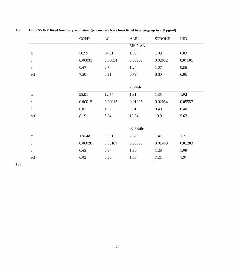
Table S5 IER fitted function parameters (parameters have been fitted to a range up to 300 µg/m³) 150

COPD LC ALRI STROKE IHD

MEDIAN

58.99 54.61 1.98 1.03 0.83

0.00031 0.00034 0.00259 0.02002 0.07101

0.67 0.74 1.24 1.07 0.55

zcf 7.58 6.91 6.79 8.80 6.86

2.5%ile

28.91 12.54 1.61 1.35 1.02

0.00015 0.00013 0.01025 0.02064 0.05557

0.83 1.02 0.81 0.49 0.40

zcf 8.19 7.24 13.84 10.91 9.62

97.5%ile

120.48 23.51 2.82 1.41 1.21

0.00028 0.00169 0.00083 0.01469 0.01283

0.63 0.67 1.50 1.26 1.09

zcf 6.02 6.56 1.50 7.21 1.97

151

23

Figure S5: Dashed line: Median and 95% CI of the relative risk (RR) as a function of exposure to PM2.5 from 1000 152 Monte Carlo samples provided by Burnett et al. (2014). Red lines: fitted curves for all-age IER functions for 5 153 mortality causes, using the parameters listed in Table S6.1 (this work). (a): Stroke, (b): Acute Lower Respiratory 154 Airways Infections (c) Chronic Obstructive Pulmonary Disease (d) Ischemaic Heart Disease (e) Lung Cancer 155

156

a b

c d

e

24

S6 Supplemental information to section 2.7 – Climate metrics 157

S6.1 calculation of aerosol optical properties and radiative forcing in TM5 158

The broadband aerosol optical properties were determined in two steps: first, the spectral optical properties in 159

the wavelength region between 0.2 µm and 5 µm were calculated on the basis of Mie theory. Only the short-to-160

infrared wave spectrum 0.2-5 μm has been considered, since the anthropogenic aerosols are most efficient in 161

scattering and absorbing the solar radiation in the submicron size range. In a second step, these spectral 162

quantities were weighted by the extra-terrestrial solar flux (Wehrli, 1985), and averaged over the applied 163

wavelength intervals of the Off-line Radiative Transfer Model (ORTM). 164

TM5 determines aerosol mass, and does not provide information about particle size distributions or particle 165

densities, so assumptions were made about these properties for the Mie calculations (Table S7.1). We assume a 166

lognormal size distribution with a geometric mean radius rg of 0.05 µm for inorganics and OC, a geometric 167

standard deviation g of 1.8 for sulphate and 2.0 for OC, and a particle density of 1600 kg.m-3

and 1200 kg.m-3

168

respectively. The optical properties of inorganics, which mainly scatter shortwave radiation, are reasonably well 169

known compared with other types of aerosols (Li et al., 2001). Wavelength-dependent complex refractive 170

indices for sulphate were taken from Toon et al. (1976). The same values were assumed for organic carbon 171

(Lund Myhre and Nielsen, 2004; Sloane, 1983). The geometric mean radius for BC particles is assumed to be 172

0.0118 mm with a sigma of 2.0 and a particle density of 1800 kg.m-3

(Penner et al., 1998). For the BC refractive 173

indices, the values from Fenn et al. (1985) were applied. We assume externally mixed aerosols and calculate the 174

forcing separately for each component. The total aerosol forcing is obtained by summing up these contributions. 175

The aerosol water content is calculated assuming equilibrium between aerosol particles and atmospheric water 176

vapour pressure at each location. The modification of aerosol specific extinction due to relative humidity of the 177

ambient air is considered using a simple approximation adapted from the data given by Nemesure et al. (1995). 178

For relative humidities (RH) below 80%, the specific extinction is enhanced by a factor of RH*0.04, assuming a 179

minimum RH of 25%. For RH exceeding 80%, the specific extinction increases exponentially with RH. The 180

factor 9.9 is reached for RH = 100%. Exponential growth is assumed for hygroscopic aerosols (ammonium salts 181

and organic carbon). Black carbon (here assumed to be externally mixed) is assumed to be mostly hydrophobic 182

and its specific extinction increases only linearly with RH. Single scattering albedo and the asymmetry factor 183

are assumed to be independent of RH. This approach might result in a small overestimation of the shortwave 184

radiative forcing of scattering aerosols, because with increasing relative humidity forward scattering is increased 185

and backscattering in space direction reduced (asymmetry factor increased). 186

25

Table S6.1 Parameters of aerosol log-normal size distributions 187

rg (µm) g Density

(kg m-3

)

Refr. index real Refr. index

imaginary

Inorganic 0.05 1.8 1600 1.53 1.0x10-7

BC 0.0118 2.0 1800 1.75 4.4x10-1

OC 0.05 2.0 1200 1.53 1.0x10-7

188

189

26

S6.2 Tables with emission-based forcing efficiencies by source region in TM5-FASST 190

Table S6.2 Regional emission-to-global forcing efficiencies for aerosol precursors (no feedback on O3 included) 191

DIRECT INDIRECT

FASST REGION FASST

CODE

W/m2/Tg

SO2

W/m²/Tg

NOx

W/m2/Tg

BC

W/m2/Tg

POM

W/m2/Tg

NH3

W/m2/Tg

SO2

N-AFR NOA -7.38E-03 -8.13E-04 5.32E-02 -1.28E-02 -0.00426 -7.19E-03

W-AFR WAF -6.74E-03 -2.91E-04 3.02E-02 -1.01E-02 -0.00242 -1.14E-02

E-AFR EAF -9.41E-03 -9.07E-04 3.22E-02 -9.92E-03 -0.00473 -1.69E-02

S-AFR SAF -8.74E-03 -1.21E-03 3.07E-02 -1.10E-02 -0.00495 -2.57E-02

REP. S. AFR RSA -4.03E-03 -4.24E-04 1.64E-02 -5.55E-03 -2.32E-03 -1.98E-02

AUSTRALIA AUS -4.20E-03 -1.03E-04 2.02E-02 -6.63E-03 -2.18E-03 -2.06E-02

NZL NZL -1.84E-03 -1.03E-04 8.12E-03 -2.84E-03 -1.25E-03 -2.42E-02

S KOREA COR -1.66E-03 -6.80E-05 1.20E-02 -4.69E-03 -3.14E-03 -3.36E-03

JAPAN JPN -1.45E-03 -9.75E-05 9.59E-03 -2.85E-03 -1.16E-03 -4.25E-03

MON+N KOREA MON -1.89E-03 -4.48E-04 1.47E-02 -5.24E-03 -1.77E-03 -3.70E-03

CHINA CHN -2.18E-03 -4.41E-04 1.67E-02 -4.93E-03 -2.24E-03 -4.90E-03

TWN TWN -2.48E-03 -3.75E-05 8.51E-03 -3.14E-03 -2.13E-03 -6.94E-03

AUT+SLV AUT -3.23E-03 -3.66E-04 2.45E-02 -6.03E-03 -2.21E-03 -3.03E-03

SWITZERLAND CHE -3.15E-03 -3.73E-04 2.39E-02 -5.74E-03 -2.70E-03 -3.07E-03

BE+NL+LUX BLX -1.63E-03 -3.43E-04 1.36E-02 -3.72E-03 -2.46E-03 -2.14E-03

SP+POR ESP -5.06E-03 -4.68E-04 2.82E-02 -8.58E-03 -3.25E-03 -5.31E-03

FIN FIN -1.38E-03 -1.18E-04 1.84E-02 -3.33E-03 -1.40E-03 -1.35E-03

FRA FRA -2.75E-03 -3.91E-04 1.87E-02 -5.56E-03 -1.88E-03 -3.30E-03

GBR+IRL GBR -1.52E-03 -1.70E-04 1.21E-02 -3.66E-03 -1.82E-03 -3.45E-03

GRC+CYP GRC -4.66E-03 -8.43E-04 3.87E-02 -9.11E-03 -2.64E-03 -3.91E-03

ITA+MLT ITA -3.97E-03 -5.40E-04 2.88E-02 -7.93E-03 -2.37E-03 -3.42E-03

GER RFA -2.16E-03 -4.24E-04 1.72E-02 -4.38E-03 -2.33E-03 -2.46E-03

SWE+DK SWE -1.47E-03 -3.77E-04 1.53E-02 -3.56E-03 -1.15E-03 -1.80E-03

NORWAY NOR -1.47E-03 -2.16E-04 1.67E-02 -3.07E-03 -6.27E-04 -4.59E-03

BULGARIA BGR -3.90E-03 -7.18E-04 3.27E-02 -7.59E-03 -2.36E-03 -3.13E-03

(continues on next page) 192

193

27

Table S6.2 Cont’d 194

DIRECT INDIRECT

FASST REGION FASST

CODE

W/m2/Tg

SO2

W/m²/Tg

NOx

W/m2/Tg

BC

W/m2/Tg

POM

W/m2/Tg

NH3

W/m2/Tg

SO2

HUN HUN -2.91E-03 -3.39E-04 2.35E-02 -5.39E-03 -2.23E-03 -2.88E-03

POL+BALTIC POL -1.96E-03 -2.01E-04 1.75E-02 -3.66E-03 -1.66E-03 -2.47E-03

REST OF C EUR RCEU -3.58E-03 -6.60E-04 3.07E-02 -7.30E-03 -1.69E-03 -3.23E-03

CZ+SLK RCZ -2.47E-03 -3.13E-04 2.14E-02 -4.90E-03 -2.46E-03 -2.63E-03

ROM ROM -3.13E-03 -4.83E-04 2.47E-02 -5.84E-03 -2.02E-03 -2.61E-03

MEX MEX -6.35E-03 -3.03E-04 1.97E-02 -7.89E-03 -3.36E-03 -1.38E-02

REST OF C AM RCAM -3.93E-03 -3.96E-04 1.53E-02 -6.57E-03 -1.90E-03 -1.01E-02

MIDDLE EAST MEME -4.83E-03 -1.49E-03 4.29E-02 -9.49E-03 -3.33E-03 -4.70E-03

EGY EGY -5.73E-03 -5.21E-04 5.64E-02 -1.21E-02 -2.93E-03 -6.05E-03

GULF REGION GLF -7.14E-03 -1.49E-03 4.40E-02 -1.08E-02 -1.61E-03 -7.80E-03

TUR TUR -4.76E-03 -4.83E-04 3.55E-02 -8.01E-03 -2.92E-03 -4.18E-03

CANADA CAN -1.80E-03 -2.87E-04 1.96E-02 -3.35E-03 -1.91E-03 -4.16E-03

USA USA -2.84E-03 -1.33E-04 1.69E-02 -5.55E-03 -2.67E-03 -5.79E-03

PAC PAC -3.25E-03 -1.03E-04 9.01E-03 -2.72E-03 -1.44E-03 -1.74E-02

KAZ KAZ -2.31E-03 -4.89E-04 2.90E-02 -4.36E-03 -2.15E-03 -4.14E-03

FRMR USSR AS RIS -2.83E-03 -2.56E-04 2.79E-02 -4.93E-03 -2.51E-03 -4.50E-03

RUS-EUR RUS -2.47E-03 -2.10E-04 2.44E-02 -4.24E-03 -1.76E-03 -3.22E-03

RUS-ASIA RUE -2.15E-03 -7.52E-04 2.58E-02 -3.91E-03 -1.12E-03 -3.90E-03

UKR UKR -2.78E-03 -3.61E-04 2.33E-02 -5.04E-03 -1.92E-03 -3.07E-03

BRAZIL BRA -5.21E-03 -1.77E-04 2.00E-02 -7.40E-03 -1.58E-03 -1.30E-02

CHL CHL -4.88E-03 -4.26E-04 2.15E-02 -6.74E-03 -1.66E-03 -2.38E-02

ARG ARG -8.75E-04 -4.26E-04 1.32E-02 -4.51E-03 -8.03E-04 -1.52E-02

REST OF S AM RSAM -5.31E-03 -9.85E-05 1.50E-02 -5.10E-03 -1.57E-03 -1.31E-02

REST OF S AS RSAS -6.46E-03 -1.41E-04 3.02E-02 -9.09E-03 -1.73E-03 -8.34E-03

(continues on next page) 195

196

28

Table S6.2 Cont’d 197

DIRECT INDIRECT

FASST REGION FASST

CODE

W/m2/Tg

SO2

W/m²/Tg

NOx

W/m2/Tg

BC

W/m2/Tg

POM

W/m2/Tg

NH3

W/m2/Tg

SO2

INDIA NDE -6.29E-03 -1.41E-04 2.61E-02 -9.37E-03 -1.59E-03 -9.66E-03

INDON IDN -3.65E-03 -4.41E-04 1.17E-02 -4.35E-03 -6.19E-04 -1.89E-02

THAIL THA -3.78E-03 -4.41E-04 1.45E-02 -5.37E-03 -1.08E-03 -1.19E-02

MALYS MYS -3.14E-03 -4.41E-04 1.32E-02 -5.02E-03 -1.16E-03 -2.63E-02

PHIL PHL -2.64E-03 -4.41E-04 8.79E-03 -3.44E-03 -1.47E-03 -1.56E-02

VTNAM VNM -2.90E-03 -4.41E-04 1.30E-02 -5.02E-03 -1.19E-03 -1.13E-02

REST OF EAS RSEA -6.16E-03 -4.41E-04 1.81E-02 -7.83E-03 -1.14E-03 -1.40E-02

SHIP SHIP -2.32E-03 -8.95E-05 1.26E-02 -2.06E-03 0.00E+00 -9.38E-03

198

29

Table S6.3: Global response in radiative forcing due to emissions of CO by including the short and long-term 199 feedback on CH4 and O3. S-O3: short-term O3 contribution M-O3: long term O3 forcing feedback via CH4 lifetime I-200 CH4: long-term feedback on CH4 via CH4 lifetime 201

CO forcing (W/m²/Tg CO)

S-O3 M-O3 I-CH4

North-America 1.20E-04 3.61E-05 8.78E-05

Europe 6.93E-05 3.95E-05 9.62E-05

South Asia 1.33E-04 4.25E-05 1.04E-04

East Asia 1.08E-04 4.27E-05 1.04E-04

Rest of the World 6.03E-05 4.36E-05 1.06E-04

202

203

Table S6.4: Global response in radiative forcing to CH4 emissions, including the long-term feedback on O3 204

CH4 forcing (W/m²/Tg CH4)

Direct CH4 O3 feedback

Globe 1.79E-03 7.16E-04

205

30

Table S6.5 Global response in radiative forcing due to regional emissions of short-lived O3 precursors - including the 206 long-term feedback on CH4 and O3. S-O3: short-term O3 contribution M-O3: long term O3 forcing feedback via CH4 207 lifetime I-CH4: long-term feedback on CH4 via CH4 lifetime. 208

Forcing (W/m²/Tg NO2) Forcing (W/m²/Tg NMVOC) Forcing (W/m²/Tg SO2)

S-O3 M-O3 I-CH4 S-O3 M-O3 I-CH4 S-O3 M-O3 I-CH4

NOA 1.20E-03 -7.63E-04 -1.86E-03 2.32E-04 1.34E-04 3.26E-04 -1.29E-04 1.28E-05 3.11E-05

WAF 1.42E-03 -9.95E-04 -2.43E-03 2.04E-04 1.26E-04 3.06E-04 -9.05E-05 1.42E-05 3.45E-05

EAF 1.28E-03 -7.96E-04 -1.94E-03 1.90E-04 1.15E-04 2.81E-04 -6.89E-05 1.68E-05 4.09E-05

SAF 1.35E-03 -7.86E-04 -1.92E-03 1.51E-04 1.24E-04 3.02E-04 -1.65E-04 2.41E-05 5.88E-05

RSA 1.27E-03 -6.99E-04 -1.70E-03 3.93E-04 3.56E-05 8.66E-05 -9.92E-05 2.33E-05 5.67E-05

AUS 2.80E-03 -1.48E-03 -3.61E-03 2.55E-04 1.40E-04 3.40E-04 -6.01E-05 1.54E-05 3.75E-05

NZL 2.95E-03 -1.95E-03 -4.77E-03 8.45E-05 1.96E-04 4.76E-04 -6.01E-05 4.11E-07 1.00E-06

COR 3.02E-04 -1.75E-04 -4.26E-04 2.92E-04 3.01E-05 7.33E-05 -2.36E-05 2.33E-06 5.68E-06

JPN 4.64E-04 -2.55E-04 -6.22E-04 2.23E-04 1.16E-04 2.82E-04 -2.18E-05 2.04E-06 4.96E-06

MON 5.36E-04 -2.89E-04 -7.03E-04 -2.77E-04 2.02E-04 4.92E-04 -2.25E-05 1.10E-06 2.69E-06

CHN 8.31E-04 -3.66E-04 -8.91E-04 2.11E-04 1.16E-04 2.82E-04 -2.22E-05 4.73E-05 1.15E-04

TWN 1.12E-03 -5.46E-04 -1.33E-03 3.49E-04 7.88E-05 1.92E-04 -4.08E-05 1.40E-06 3.41E-06

AUT 2.54E-04 -1.60E-04 -3.89E-04 2.19E-04 1.12E-04 2.74E-04 -4.23E-05 7.20E-07 1.75E-06

CHE 3.36E-04 -1.89E-04 -4.60E-04 2.22E-04 1.18E-04 2.86E-04 -2.65E-05 1.27E-07 3.10E-07

BLX 8.16E-05 -7.31E-05 -1.78E-04 2.01E-04 1.20E-04 2.91E-04 -1.76E-05 4.66E-07 1.14E-06

ESP 4.89E-04 -3.01E-04 -7.32E-04 2.22E-04 1.14E-04 2.77E-04 -6.54E-05 1.56E-05 3.80E-05

FIN 1.57E-04 -1.40E-04 -3.40E-04 1.60E-04 1.18E-04 2.87E-04 -1.30E-05 1.69E-07 4.13E-07

FRA 2.46E-04 -1.59E-04 -3.87E-04 2.14E-04 1.15E-04 2.79E-04 -3.69E-05 2.50E-06 6.09E-06

GBR 7.17E-05 -8.03E-05 -1.95E-04 2.01E-04 1.22E-04 2.96E-04 -1.69E-05 2.63E-06 6.40E-06

GRC 4.74E-04 -2.87E-04 -7.00E-04 2.70E-04 4.62E-05 1.13E-04 -7.23E-05 5.13E-06 1.25E-05

ITA 3.58E-04 -2.04E-04 -4.97E-04 2.46E-04 8.61E-05 2.10E-04 -5.68E-05 5.76E-06 1.40E-05

RFA 1.29E-04 -9.65E-05 -2.35E-04 1.98E-04 1.17E-04 2.84E-04 -2.28E-05 1.82E-06 4.44E-06

SWE 1.94E-04 -1.60E-04 -3.90E-04 1.60E-04 1.17E-04 2.84E-04 -1.17E-05 2.12E-07 5.16E-07

NOR 4.20E-04 -3.01E-04 -7.33E-04 1.35E-04 1.03E-04 2.50E-04 -1.38E-05 9.75E-07 2.37E-06

BGR 3.63E-04 -2.24E-04 -5.46E-04 2.39E-04 9.99E-05 2.43E-04 -5.05E-05 6.36E-06 1.55E-05

209

31

Table S6.5 – Cont’d

Forcing (W/m²/Tg NO2) Forcing (W/m²/Tg NMVOC) Forcing (W/m²/Tg SO2)

S-O3 M-O3 I-CH4 S-O3 M-O3 I-CH4 S-O3 M-O3 I-CH4

HUN 2.14E-04 -1.42E-04 -3.46E-04 2.07E-04 1.17E-04 2.84E-04 -3.39E-05 1.95E-06 4.75E-06

POL 1.67E-04 -1.20E-04 -2.92E-04 1.93E-04 1.10E-04 2.67E-04 -2.16E-05 4.41E-06 1.07E-05

RCEU 4.17E-04 -2.47E-04 -6.02E-04 2.00E-04 1.24E-04 3.01E-04 -4.56E-05 6.86E-06 1.67E-05

RCZ 1.72E-04 -1.21E-04 -2.95E-04 2.05E-04 1.09E-04 2.66E-04 -2.78E-05 1.27E-06 3.10E-06

ROM 2.52E-04 -1.44E-04 -3.51E-04 2.15E-04 1.17E-04 2.86E-04 -3.63E-05 2.16E-06 5.26E-06

EUR 2.37E-04 -1.59E-04 -3.87E-04 2.01E-04 1.54E-05 3.74E-05 -3.98E-05 5.90E-05 1.44E-04

MEX 1.67E-03 -8.98E-04 -2.19E-03 2.38E-04 1.17E-04 2.84E-04 -9.34E-05 3.15E-05 7.67E-05

RCAM 2.12E-03 -1.22E-03 -2.97E-03 2.08E-04 1.43E-04 3.49E-04 -5.67E-05 5.69E-06 1.39E-05

MEME 5.71E-04 -3.17E-04 -7.72E-04 2.73E-04 1.00E-04 2.44E-04 -1.06E-04 1.05E-05 2.55E-05

EGY 7.14E-04 -4.89E-04 -1.19E-03 3.28E-04 6.19E-05 1.51E-04 -1.13E-04 7.85E-06 1.91E-05

GOLF 1.28E-03 -7.11E-04 -1.73E-03 2.03E-04 1.47E-04 3.59E-04 -1.18E-04 7.70E-05 1.87E-04

TUR 5.69E-04 -3.07E-04 -7.48E-04 2.53E-04 1.01E-04 2.46E-04 -8.00E-05 1.52E-05 3.71E-05

CAN 4.83E-04 -2.85E-04 -6.94E-04 1.39E-04 1.32E-04 3.22E-04 -3.13E-05 8.27E-06 2.01E-05

USA 4.72E-04 -2.39E-04 -5.81E-04 2.35E-04 1.09E-04 2.66E-04 -5.73E-05 8.43E-05 2.05E-04

PAC 4.91E-03 -2.33E-03 -5.69E-03 1.50E-04 1.96E-04 4.77E-04 -4.21E-05 3.75E-07 9.13E-07

KAZ 6.52E-04 -3.36E-04 -8.18E-04 1.57E-04 1.22E-04 2.98E-04 -2.56E-05 5.21E-06 1.27E-05

RIS 7.94E-04 -3.66E-04 -8.93E-04 2.12E-04 1.35E-04 3.28E-04 -4.48E-05 1.48E-06 3.61E-06

RUS 2.93E-04 -1.97E-04 -4.80E-04 1.80E-04 1.26E-04 3.07E-04 -2.16E-05 1.02E-05 2.49E-05

RUE 6.96E-04 -4.02E-04 -9.80E-04 1.11E-04 1.24E-04 3.01E-04 -3.42E-05 5.25E-06 1.28E-05

UKR 2.56E-04 -1.66E-04 -4.04E-04 2.08E-04 1.24E-04 3.03E-04 -3.50E-05 6.48E-06 1.58E-05

BRA 2.84E-03 -1.30E-03 -3.16E-03 8.43E-05 1.41E-04 3.43E-04 -6.90E-05 1.45E-05 3.54E-05

CHL 2.13E-03 -1.30E-03 -3.18E-03 3.06E-04 7.81E-05 1.90E-04 -1.14E-04 1.14E-05 2.77E-05

ARG 2.95E-03 -1.44E-03 -3.52E-03 1.10E-04 1.58E-04 3.84E-04 -1.14E-04 1.93E-06 4.71E-06

RSAM 2.79E-03 -1.52E-03 -3.71E-03 1.33E-04 1.44E-04 3.50E-04 -6.78E-05 7.48E-06 1.82E-05

RSAS 1.20E-03 -5.60E-04 -1.36E-03 2.22E-04 1.32E-04 3.21E-04 -5.08E-05 7.69E-06 1.87E-05

NDE 1.18E-03 -5.97E-04 -1.45E-03 2.59E-04 1.31E-04 3.18E-04 -5.08E-05 4.27E-05 1.04E-04

IDN 2.23E-03 -1.25E-03 -3.05E-03 2.19E-04 1.57E-04 3.83E-04 -4.21E-05 1.01E-05 2.46E-05

210

32

Table S6.5 – Cont’d

Forcing (W/m²/Tg NO2) Forcing (W/m²/Tg NMVOC) Forcing (W/m²/Tg SO2)

S-O3 M-O3 I-CH4 S-O3 M-O3 I-CH4 S-O3 M-O3 I-CH4

THA 1.90E-03 -9.83E-04 -2.40E-03 2.22E-04 1.37E-04 3.33E-04 -4.21E-05 4.81E-06 1.17E-05

MYS 2.23E-03 -1.18E-03 -2.87E-03 2.54E-04 1.47E-04 3.59E-04 -4.21E-05 2.36E-06 5.76E-06

PHL 2.29E-03 -1.07E-03 -2.61E-03 3.57E-04 1.57E-04 3.82E-04 -4.21E-05 6.33E-06 1.54E-05

VNM 2.03E-03 -1.04E-03 -2.53E-03 2.14E-04 1.60E-04 3.91E-04 -4.21E-05 9.48E-07 2.31E-06

RSEA 1.40E-03 -8.07E-04 -1.97E-03 1.48E-04 1.40E-04 3.41E-04 -4.21E-05 8.35E-07 2.03E-06

SHIP 1.40E-03 -8.46E-04 -2.06E-03 0.00E+00 0.00E+00 0.00E+00 -2.87E-05 3.64E-05 8.87E-05

AIR 4.25E-03 -1.14E-03 -2.77E-03 0.00E+00 0.00E+00 0.00E+00 0.00E+00 0.00E+00 0.00E+00

211

33

Table S6.6 Year 2000 global anthropogenic forcing (W/m²) by component from TM5-FASST, versus values reported 212 in AR5 (1750 – 2011). Large scale forest fires have not been included. 213

CH4

BC

PM2.5

OC

PM2.5

O3

(SS)

O3

(PM)

NO3

PM2.5

SO4

PM2.5 INDIR TOT

CH4 AR5 0.641 0.24 0.88

FASST 0.500 0.20 0.70

CO AR5 0.072 0.075 0.15

FASST 0.083 0.074 0.034 0.19

NMVOC AR5 0.025 0.042 0.07

FASST 0.049 0.033 0.020 0.10

NOx AR5 -0.245 0.14 -0.040 -0.14

FASST -0.167 0.13 -0.068 -0.040 -0.15

NH3 AR5 -0.070 0.01 -0.06

FASST -0.091 -0.09

BC AR5 0.60 0.60

FASST 0.15 0.15

OC AR5 -0.29 -0.29

FASST -0.24 -0.24

SO2 AR5 -0.41 -0.21

FASST -0.37 -0.37

INDIRECT

AEROSOLS

AR5 -0.45 -0.45

FASST -0.81 -0.81

214

34

Figure S6.1: Annual average radiative forcing efficiencies for SO4, Particulate Organic Matter, Black carbon, and 215 the indirect forcing associated with SO4 [W/(m2*mg]. a-b-c: direct SO4, POM, BC (upper legend); d: indirect SO4 216 (lower legend) 217

218

b a

c d

35

219

Figure S6.2 TM5-FASST break-down of direct radiative forcing by sector by emitted component, based on RCP year 220 2000 emission inventory by sector. 221

222

36

S7 Supplemental Figures to section 3.1 - Validation against the full TM5 model: additivity and linearity

PM2.5 additivity of simultaneous SO2 + NOx -20% emission perturbation responses

Figure S7.1 Secondary PM2.5 species response to SO2 and NOx -20% emission perturbations. Y-axis: summed individual

perturbations (P2 + P3) X-axis: response to combined perturbation (P1). All results are obtained with TM5-CTM. (a): sulfate

(b) nitrate (c) ammonium (d) sum of all 3 components

5

a b

c d

37

Figure S7.2: Relative error in country/region annual average PM2.5 (including primary and secondary components) compared

to TM5-CTM by linear extrapolation of a -20% emission perturbation of SO2 (a), NOx (b) and NH3 (c) to -80% (blue dots) and

+100% (red dots) respectively for representative source/receptor regions, and the relative error on PM2.5 by extrapolation of

all 3 precursor emissions simultaneously (d) (as sum of the 3 individual contributions). For the European receptor regions, the

perturbation was made over all sub-regions simultaneously. 5

a b

c d

38

Figure S7.3 TM5 O3 (a) and O3 metrics M6M (b), AOT40 (c) and M12 (d) responses to simultaneous SO2 and NOx

perturbations including the -80%, -20% and +100% perturbation outcomes for the limited set of source regions. Y-axis:

calculated as the sum of the individual responses; X-axis: evaluated from simultaneous perturbation. 5

a b

c d

39

Figure S7.4 Relative error on TM5-FASSST computed (base + perturbation response) annual O3 (a), and M6M (b), M12 (c),

AOT40 (d) exposure metrics relative to TM5 for individual emission perturbations of NOx of -80% (blue symbols) and +100%

(red symbols) relative to the base simulation

a b

c d

40

Figure S7.5 Same as Fig S7.4, now for NMVOC perturbations

a b

c d

41

Figure S7.6 Same as Fig. S7.4, now for combined NOx+NMVOC perturbations

a b

c d

42

S8 Supplemental information to section 3.2 - TM5-FASST_v0 versus TM5 for future emission scenarios

S8.1 Major features of the Global Energy Assesment scenarios used in the validation study

The GEA scenarios (Riahi, Dentener et al. 2012), consistent with similar long-term climate outcomes as the RCPs, are

implemented in the MESSAGE model (Messner and Strubegger 1995; Riahi, Gruebler et al. 2007) and include more

detailed representation of short-term air quality legislations from the GAINS model (Amann et al., 2011). A number of 5

air pollutants are included in the scenario (SO2, NOx, CO, VOCs, BC, OC, total primary PM2.5) air pollutants and are

available at 0.5o x 0.5

o resolution based on inventory data described in Lamarque et al. (2010), and an exposure-driven

algorithm for the downscaling of the regional air-pollutant emissions projections. The GEA scenarios have been used to

estimate global health impacts of outdoor air pollution (Rao et al., 2012, 2013) as well as for regional impacts analysis

(Colette et al., 2012, 2013). We evaluate following pair: 10

1. FLE-2030 (Fixed Legislation scenario): This is a scenario with no improvement in air quality legislations

beyond 2005. It thus serves to indicate a scenario with failure in terms of implementation of future air quality

and climate policies and is used as a worst-case scenario, defining an upper boundary for the range of plausible

air pollutant emission scenarios until 2030. In the literature this kind of scenarios is also referred to as Frozen

legislation, or no-further-controls (NFC). 15

2. MIT-2030 (MITigation scenario): This scenario, consistent with long-term climate outcomes of the RCP2.6,

assumes stringent climate mitigation policies consistent with a target of 2oC global warming by the end of the

century (2100), combined with stringent air quality legislations (SLE). Thus the MIT-2030 scenario provides a

best-case scenario, defining the lower boundary of pollutant emission strengths. We evaluate the outcome in the

year 2030. 20

43

Table S8: Relative emission changes for the test scenarios MIT-2030 and FLE-2030 compared to the year 2000 base scenario

used for the 20% perturbation simulations.

BC NH3 NOx POM SO2 NMVOC PM2.5

MIT-2030

ASIA -47% +19% -30% -49% -61% -35% +26%

LAM -83% -61% -83% -68% -86% -75% -65%

MAF -57% -60% -58% -31% -79% -43% -31%

OECD90 -89% -41% -73% -80% -90% -81% -74%

REF -91% -64% -83% -71% -91% -83% -70%

GLOBAL -49% +25% -64% -36% -72% -39% -6%

FLE-2030

ASIA +97% +21% +165% +20% +98% +53% +245%

LAM -74% -61% -60% -66% -72% -54% -59%

MAF +7% -59% -7% +20% -17% +44% +18%

OECD90 -72% -40% -12% -74% -32% -67% -56%

REF -82% -64% -53% -66% -51% -73% -58%

GLOBAL +45% +27% +11% +7% +29% +33% +94%

OECD90: All countries that belonged to the Organization of Economic Development (OECD) as of 1990

MAF: Developing Countries in Middle East & Africa

LA:, All developing countries in Latin America 5

REF: Countries undergoing economic reform - East European countries and the Newly Independent States of the former Soviet Union

ASIA: All developing countries in Asia

44

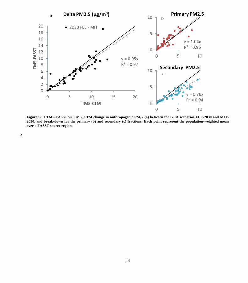
Figure S8.1 TM5-FASST vs. TM5_CTM change in anthropogenic PM2.5 (a) between the GEA scenarios FLE-2030 and MIT-

2030, and break-down for the primary (b) and secondary (c) fractions. Each point represent the population-weighted mean

over a FASST source region.

5

a b

c

45

Figure S8.2 TM5-FASST versus TM5-CTM change in annual mean ozone (a) and exposure metric M6M (b) between the GEA

scenarios FLE-2030 and MIT-2030. Each point represents the population-weighted mean over a FASST source region.

a b

46

S9 Supplemental figures to section 3.3.4 - Health impacts: intercomparison with ACCMIP model ensemble

RCP 2.6 RCP 4.5 RCP 8.5

Figure S9: Mortality burden (million deaths) from PM2.5 in 2030 and 2050 for RCP scenarios RCP 2.6 (a, d). RCP 4.5 (b, e)

and RCP8.5 (c, f) relative to exposure to year 2000 concentrations, for North America (a to c) Europe and Europe (d to f). 5 Blue bars: Mean of ACCMIP model ensemble results (Silva et al., 2016). Red bars: TM5-FASST.

a b c

d e f

47

RCP 2.6 RCP 4.5 RCP 8.5

Figure S10: As in Fig. S9, now for regions East Asia (a to c), India (d to f) and the globe (g to i)

a b c

d e f

g h i

48

Supplemental Information - References

Amann, M., Bertok, I., Borken-Kleefeld, J., Cofala, J., Heyes, C., Höglund-Isaksson, L., Klimont, Z., Nguyen, B.,

Posch, M., Rafaj, P., Sandler, R., Schöpp, W., Wagner, F. and Winiwarter, W.: Cost-effective control of air quality and

greenhouse gases in Europe: Modeling and policy applications, Environ. Model. Softw., 26(12), 1489–1501,

doi:10.1016/j.envsoft.2011.07.012, 2011. 5

Bergamaschi, P., Krol, M., Dentener, F., Vermeulen, A., Meinhardt, F., Graul, R., Ramonet, M., Peters, W. and

Dlugokencky, E. J.: Inverse modelling of national and European CH4 emissions using the atmospheric zoom model

TM5, Atmospheric Chem. Phys., 5(9), 2431–2460, 2005.

Brauer, M., Amann, M., Burnett, R. T., Cohen, A., Dentener, F., Ezzati, M., Henderson, S. B., Krzyzanowski, M.,

Martin, R. V., Van Dingenen, R., Van Donkelaar, A. and Thurston, G. D.: Exposure assessment for estimation of the 10

global burden of disease attributable to outdoor air pollution, Environ. Sci. Technol., 46(2), 652–660,

doi:10.1021/es2025752, 2012.

Brauer, M., Freedman, G., Frostad, J., Van, D., Martin, R. V., Dentener, F., Dingenen, R. V., Estep, K., Amini, H., Apte,

J. S., Balakrishnan, K., Barregard, L., Broday, D., Feigin, V., Ghosh, S., Hopke, P. K., Knibbs, L. D., Kokubo, Y., Liu,

Y., Ma, S., Morawska, L., Sangrador, J. L. T., Shaddick, G., Anderson, H. R., Vos, T., Forouzanfar, M. H., Burnett, R. 15

T. and Cohen, A.: Ambient Air Pollution Exposure Estimation for the Global Burden of Disease 2013, Environ. Sci.

Technol., 50(1), 79–88, doi:10.1021/acs.est.5b03709, 2016.

Burnett, R. T., Pope, C. A., III, Ezzati, M., Olives, C., Lim, S. S., Mehta, S., Shin, H. H., Singh, G., Hubbell, B., Brauer,

M., Anderson, H. R., Smith, K. R., Balmes, J. R., Bruce, N. G., Kan, H., Laden, F., Prüss-Ustün, A., Turner, M. C.,

Gapstur, S. M., Diver, W. R. and Cohen, A.: An Integrated Risk Function for Estimating the Global Burden of Disease 20

Attributable to Ambient Fine Particulate Matter Exposure, Environ. Health Perspect., doi:10.1289/ehp.1307049, 2014.

CIESIN: Gridded Population of the World Version 3 (GPWv3), [online] Available from:

http://sedac.ciesin.columbia.edu/gpw (Accessed 12 September 2012), 2005.

Cohen, A. J., Brauer, M., Burnett, R., Anderson, H. R., Frostad, J., Estep, K., Balakrishnan, K., Brunekreef, B.,

Dandona, L., Dandona, R., Feigin, V., Freedman, G., Hubbell, B., Jobling, A., Kan, H., Knibbs, L., Liu, Y., Martin, R., 25

Morawska, L., Pope, C. A., III, Shin, H., Straif, K., Shaddick, G., Thomas, M., van Dingenen, R., van Donkelaar, A.,

Vos, T., Murray, C. J. L. and Forouzanfar, M. H.: Estimates and 25-year trends of the global burden of disease

attributable to ambient air pollution: an analysis of data from the Global Burden of Diseases Study 2015, The Lancet,

389(10082), 1907–1918, doi:10.1016/S0140-6736(17)30505-6, 2017.

Colette, A., Granier, C., Hodnebrog, ø., Jakobs, H., Maurizi, A., Nyiri, A., Rao, S., Amann, M., Bessagnet, B., 30

D’Angiola, A., Gauss, M., Heyes, C., Klimont, Z., Meleux, F., Memmesheimer, M., Mieville, A., Rouïl, L., Russo, F.,

Schucht, S., Simpson, D., Stordal, F., Tampieri, F. and Vrac, M.: Future air quality in Europe: A multi-model assessment

of projected exposure to ozone, Atmospheric Chem. Phys., 12(21), 10613–10630, doi:10.5194/acp-12-10613-2012,

2012.

Colette, A., Bessagnet, B., Vautard, R., Szopa, S., Rao, S., Schucht, S., Klimont, Z., Menut, L., Clain, G., Meleux, F., 35

Curci, G. and Rouïl, L.: European atmosphere in 2050, a regional air quality and climate perspective under CMIP5

scenarios, Atmospheric Chem. Phys., 13(15), 7451–7471, doi:10.5194/acp-13-7451-2013, 2013.

Crippa, M., Janssens-Maenhout, G., Dentener, F., Guizzardi, D., Sindelarova, K., Muntean, M., Van Dingenen, R. and

Granier, C.: Forty years of improvements in European air quality: Regional policy-industry interactions with global

impacts, Atmospheric Chem. Phys., 16(6), 3825–3841, doi:10.5194/acp-16-3825-2016, 2016. 40

49

Dana, M. T. and Hales, J. M.: Statistical aspects of the washout of polydisperse aerosols, Atmospheric Environ. 1967,

10(1), 45–50, doi:10.1016/0004-6981(76)90258-4, 1976.

De Meij, A., Krol, M., Dentener, F., Vignati, E., Cuvelier, C. and Thunis, P.: The sensitivity of aerosol in Europe to two

different emission inventories and temporal distribution of emissions, Atmospheric Chem. Phys., 6(12), 4287–4309,

2006. 5

Dentener, F., Drevet, J., Lamarque, J. F., Bey, I., Eickhout, B., Fiore, A. M., Hauglustaine, D., Horowitz, L. W., Krol,

M., Kulshrestha, U. C., Lawrence, M., Galy-Lacaux, C., Rast, S., Shindell, D., Stevenson, D., Van Noije, T., Atherton,

C., Bell, N., Bergman, D., Butler, T., Cofala, J., Collins, B., Doherty, R., Ellingsen, K., Galloway, J., Gauss, M.,

Montanaro, V., Müller, J. F., Pitari, G., Rodriguez, J., Sanderson, M., Solmon, F., Strahan, S., Schultz, M., Sudo, K.,

Szopa, S. and Wild, O.: Nitrogen and sulfur deposition on regional and global scales: A multimodel evaluation, Glob. 10

Biogeochem. Cycles, 20(4), GB4003, doi:10.1029/2005GB002672, 2006.

van Donkelaar, A., Martin, R. V., Brauer, M., Hsu, N. C., Kahn, R. A., Levy, R. C., Lyapustin, A., Sayer, A. M. and

Winker, D. M.: Global Estimates of Fine Particulate Matter using a Combined Geophysical-Statistical Method with

Information from Satellites, Models, and Monitors, Environ. Sci. Technol., 50(7), 3762–3772,

doi:10.1021/acs.est.5b05833, 2016. 15

Fenn, R. W., Clough, S. A., Gallery, W. O., Good, R. E., Kneizys, F. X., Mill, J. D., Rothman, L. S., Shettle, E. P. and

Volz, F. E.: Optical and infrared properties of the atmosphere, in Handbook of Geophysics and the Space Environment,

vol. 18, pp. 1–27, Air Force Geophys. Lab., Hanscom Air Force Base, Bedford, Mass., 1985.

Ganzeveld, L. and Lelieveld, J.: Dry deposition parameterization in a chemistry general circulation model and its

influence on the distribution of reactive trace gases, J. Geophys. Res., 100(D10), 20,999-21,012, 1995. 20

GEA: Global Energy Assessment - Toward a Sustainable Future, Cambridge University Press, Cambridge, UK and New

York, NY, USA and the International Institute for Applied Systems Analysis, Laxenburg, Austria. [online] Available

from: www.globalenergyassessment.org, 2012.

Gery, M. W., Whitten, G. Z., Killus, J. P. and Dodge, M. C.: A photochemical kinetics mechanism for urban and

regional scale computer modeling, J. Geophys. Res., 94(D10), 12,925-12,956, 1989a. 25

Gery, M. W., Edmond, R. D. and Whitten, G. Z.: Potential effects of stratospheric ozone depletion and global

temperature rise on urban photochemistry, Stud. Environ. Sci., 35(C), 365–375, doi:10.1016/S0166-1116(08)70604-6,

1989b.

Guelle, W., Balkanski, Y. J., Dibb, J. E., Schulz, M. and Dulac, F.: Wet deposition in a global size-dependent aerosol

transport model 2. Influence of the scavenging scheme on 210Pb vertical profiles, surface concentrations, and 30

deposition, J. Geophys. Res. Atmospheres, 103(D22), 28875–28891, 1998.

Hertel, O., Berkowicz, R., Christensen, J. and Hov, Ø.: Test of two numerical schemes for use in atmospheric transport-

chemistry models, Atmospheric Environ. Part Gen. Top., 27(16), 2591–2611, doi:10.1016/0960-1686(93)90032-T,

1993.

Houweling, S., Dentener, F. and Lelieveld, J.: The impact of nonmethane hydrocarbon compounds on tropospheric 35

photochemistry, J. Geophys. Res. Atmospheres, 103(3339), 10673–10696, 1998.

Huijnen, V., Williams, J., van Weele, M., van Noije, T., Krol, M., Dentener, F., Segers, A., Houweling, S., Peters, W.,

de Laat, J., Boersma, F., Bergamaschi, P., van Velthoven, P., Le Sager, P., Eskes, H., Alkemade, F., Scheele, R.,

50

Nédélec, P. and Pätz, H.-W.: The global chemistry transport model TM5: description and evaluation of the tropospheric

chemistry version 3.0, Geosci. Model Dev., 3(2), 445–473, doi:10.5194/gmd-3-445-2010, 2010.

Jeuken, A., Veefkind, J. P., Dentener, F., Metzger, S. and Robles, G.: Simulation of the aerosol optical depth over

Europe for August 1997 and a comparison with observations, J. Geophys. Res. Atmospheres, 106(D22), 28295–28311,

2001. 5

Kitous, A., Keramidas, K., Vandyck, T., Saveyn, B., Van Dingenen, R., Spadaro, J. and Holland, M.: Global Energy and

Climate Outlook 2017: How climate policies improve air quality, Joint Research Centre (Seville site)., 2017.

Krol, M., Houweling, S., Bregman, B., van den Broek, M., Segers, A., van Velthoven, P., Peters, W., Dentener, F. and

Bergamaschi, P.: The two-way nested global chemistry-transport zoom model TM5: algorithm and applications, Atmos

Chem Phys, 5(2), 417–432, doi:10.5194/acp-5-417-2005, 2005. 10

Kuylenstierna, J. C. I., Zucca, M. C., Amann, M., Cardenas, B., Chambers, B., Klimont, Z., Hicks, K., Mills, R., Molina,

L., Murray, F., Pearson, P., Sethi, S., Shindell, D., Sokona, Y., Terry, S., Vallack, H., Van Dingenen, R., Williams, M.,

Wilson, C. and Zusman, E.: Near-term climate protection and clean air benefits: Actions for controlling short-lived

climate forcers, Report, United Nations Environment Programme, Nairobi, Kenya. [online] Available from:

http://researchrepository.murdoch.edu.au/id/eprint/15325/ (Accessed 10 January 2017), 2011. 15

Lamarque, J.-F., Bond, T. C., Eyring, V., Granier, C., Heil, A., Klimont, Z., Lee, D., Liousse, C., Mieville, A., Owen,

B., Schultz, M. G., Shindell, D., Smith, S. J., Stehfest, E., Van, A., Cooper, O. R., Kainuma, M., Mahowald, N.,

McConnell, J. R., Naik, V., Riahi, K. and Van, V.: Historical (1850-2000) gridded anthropogenic and biomass burning

emissions of reactive gases and aerosols: Methodology and application, Atmospheric Chem. Phys., 10(15), 7017–7039,

doi:10.5194/acp-10-7017-2010, 2010. 20

Li, J., Wong, J. G. D., Dobbie, J. S. and Chýlek, P.: Parameterization of the optical properties of sulfate aerosols, J.

Atmospheric Sci., 58(2), 193–209, 2001.

Lim, S. S., Vos, T., Flaxman, A. D., Danaei, G., Shibuya, K., Adair-Rohani, H., Amann, M., Anderson, H. R., Andrews,

K. G., Aryee, M., Atkinson, C., Bacchus, L. J., Bahalim, A. N., Balakrishnan, K., Balmes, J., Barker-Collo, S., Baxter,

A., Bell, M. L., Blore, J. D., Blyth, F., Bonner, C., Borges, G., Bourne, R., Boussinesq, M., Brauer, M., Brooks, P., 25

Bruce, N. G., Brunekreef, B., Bryan-Hancock, C., Bucello, C., Buchbinder, R., Bull, F., Burnett, R. T., Byers, T. E.,

Calabria, B., Carapetis, J., Carnahan, E., Chafe, Z., Charlson, F., Chen, H., Chen, J. S., Cheng, A. T.-A., Child, J. C.,

Cohen, A., Colson, K. E., Cowie, B. C., Darby, S., Darling, S., Davis, A., Degenhardt, L., Dentener, F., Des Jarlais, D.

C., Devries, K., Dherani, M., Ding, E. L., Dorsey, E. R., Driscoll, T., Edmond, K., Ali, S. E., Engell, R. E., Erwin, P. J.,

Fahimi, S., Falder, G., Farzadfar, F., Ferrari, A., Finucane, M. M., Flaxman, S., Fowkes, F. G. R., Freedman, G., 30

Freeman, M. K., Gakidou, E., Ghosh, S., Giovannucci, E., Gmel, G., Graham, K., Grainger, R., Grant, B., Gunnell, D.,

Gutierrez, H. R., Hall, W., Hoek, H. W., Hogan, A., Hosgood III, H. D., Hoy, D., Hu, H., Hubbell, B. J., Hutchings, S.

J., Ibeanusi, S. E., Jacklyn, G. L., Jasrasaria, R., Jonas, J. B., Kan, H., Kanis, J. A., Kassebaum, N., Kawakami, N.,

Khang, Y.-H., Khatibzadeh, S., Khoo, J.-P., Kok, C., et al.: A comparative risk assessment of burden of disease and

injury attributable to 67 risk factors and risk factor clusters in 21 regions, 1990-2010: A systematic analysis for the 35

Global Burden of Disease Study 2010, The Lancet, 380(9859), 2224–2260, doi:10.1016/S0140-6736(12)61766-8, 2012.

Lund Myhre, C. E. and Nielsen, C. J.: Optical properties in the UV and visible spectral region of organic acids relevant

to tropospheric aerosols, Atmos Chem Phys, 4(7), 1759–1769, doi:10.5194/acp-4-1759-2004, 2004.

Nemesure, S., Wagener, R. and Schwartz, S. E.: Direct shortwave forcing of climate by the anthropogenic sulfate

aerosol: Sensitivity to particle size, composition, and relative humidity, J. Geophys. Res. Atmospheres, 100(D12), 40

26105–26116, doi:10.1029/95JD02897, 1995.

51

van Noije, T. P. C., Eskes, H. J., Dentener, F. J., Stevenson, D. S., Ellingsen, K., Schultz, M. G., Wild, O., Amann, M.,

Atherton, C. S., Bergmann, D. J., Bey, I., Boersma, K. F., Butler, T., Cofala, J., Drevet, J., Fiore, A. M., Gauss, M.,

Hauglustaine, D. A., Horowitz, L. W., Isaksen, I. S. A., Krol, M. C., Lamarque, J.-F., Lawrence, M. G., Martin, R. V.,

Montanaro, V., Müller, J.-F., Pitari, G., Prather, M. J., Pyle, J. A., Richter, A., Rodriguez, J. M., Savage, N. H., Strahan,

S. E., Sudo, K., Szopa, S. and van Roozendael, M.: Multi-model ensemble simulations of tropospheric NO2 compared 5

with GOME retrievals for the year 2000, Atmos Chem Phys, 6(10), 2943–2979, doi:10.5194/acp-6-2943-2006, 2006.

OECD: The Economic Consequences of Outdoor Air Pollution, OECD Publishing. [online] Available from:

http://www.oecd-ilibrary.org/environment/the-economic-consequences-of-outdoor-air-pollution_9789264257474-en

(Accessed 10 January 2017), 2016.

Penner, J. E., Chuang, C. C. and Grant, K.: Climate forcing by carbonaceous and sulfate aerosols, Clim. Dyn., 14(12), 10

839–851, doi:10.1007/s003820050259, 1998.

Peters, W.: Toward regional-scale modeling using the two-way nested global model TM5: Characterization of transport

using SF 6, J. Geophys. Res., 109(D19), doi:10.1029/2004JD005020, 2004.

Petersen, A. C., Spee, E. J., Van, D. and Hundsdorfer, W.: An evaluation and intercomparison of four new advection

schemes for use in global chemistry models, J. Geophys. Res. Atmospheres, 103(D15), 19253–19269, 1998. 15

Rao, S., Chirkov, V., Dentener, F., Van Dingenen, R., Pachauri, S., Purohit, P., Amann, M., Heyes, C., Kinney, P., Kolp,

P., Klimont, Z., Riahi, K. and Schoepp, W.: Environmental Modeling and Methods for Estimation of the Global Health

Impacts of Air Pollution, Environ. Model. Assess., 17(6), 613–622, doi:10.1007/s10666-012-9317-3, 2012.

Rao, S., Pachauri, S., Dentener, F., Kinney, P., Klimont, Z., Riahi, K. and Schoepp, W.: Better air for better health:

Forging synergies in policies for energy access, climate change and air pollution, Glob. Environ. Change, 23(5), 1122–20

1130, doi:10.1016/j.gloenvcha.2013.05.003, 2013.

Rao, S., Klimont, Z., Leitao, J., Riahi, K., Van Dingenen, R., Reis, L. A., Katherine Calvin, Dentener, F., Drouet, L.,

Fujimori, S., Harmsen, M., Luderer, G., Chris Heyes, Strefler, J., Tavoni, M. and Vuuren, D. P. van: A multi-model

assessment of the co-benefits of climate mitigation for global air quality, Environ. Res. Lett., 11(12), 124013,

doi:10.1088/1748-9326/11/12/124013, 2016. 25

Rao, S., Klimont, Z., Smith, S. J., Van Dingenen, R., Dentener, F., Bouwman, L., Riahi, K., Amann, M., Bodirsky, B.

L., van Vuuren, D. P., Aleluia Reis, L., Calvin, K., Drouet, L., Fricko, O., Fujimori, S., Gernaat, D., Havlik, P.,

Harmsen, M., Hasegawa, T., Heyes, C., Hilaire, J., Luderer, G., Masui, T., Stehfest, E., Strefler, J., van der Sluis, S. and

Tavoni, M.: Future air pollution in the Shared Socio-economic Pathways, Glob. Environ. Change, 42, 346–358,

doi:10.1016/j.gloenvcha.2016.05.012, 2017. 30

Riahi, K., Dentener, F., Gielen, D., Grubler, A., Jewell, J., Klimont, Z., Krey, V., McCollum, D., Pachauri, S., Rao, S.,

van Ruijven, B., van Vuuren, D. P. and Wilson, C.: The Global Energy Assessment - Chapter 17 - Energy Pathways for

Sustainable Development, in Global Energy Assessment - Toward a Sustainable Future, pp. 1203–1306, Cambridge

University Press, Cambridge, UK and New York, NY, USA and the International Institute for Applied Systems

Analysis, Laxenburg, Austria. [online] Available from: www.globalenergyassessment.org, 2012. 35

Russell, G. L. and Lerner, J. A.: A New Finite-Differencing Scheme for the Tracer Transport Equation, J. Appl.

Meteorol., 20(12), 1483–1498, doi:10.1175/1520-0450(1981)020<1483:ANFDSF>2.0.CO;2, 1981.

Shindell, D. T., Chin, M., Dentener, F., Doherty, R. M., Faluvegi, G., Fiore, A. M., Hess, P., Koch, D. M., MacKenzie, I.

A., Sanderson, M. G., Schultz, M. G., Schulz, M., Stevenson, D. S., Teich, H., Textor, C., Wild, O., Bergmann, D. J.,

Bey, I., Bian, H., Cuvelier, C., Duncan, B. N., Folberth, G., Horowitz, L. W., Jonson, J., Kaminski, J. W., Marmer, E., 40

52

Park, R., Pringle, K. J., Schroeder, S., Szopa, S., Takemura, T., Zeng, G., Keating, T. J. and Zuber, A.: A multi-model

assessment of pollution transport to the Arctic, Atmos Chem Phys, 8(17), 5353–5372, doi:10.5194/acp-8-5353-2008,

2008.

Silva, R. A., West, J. J., Lamarque, J. F., Shindell, D. T., Collins, W. J., Dalsoren, S., Faluvegi, G., Folberth, G.,

Horowitz, L. W., Nagashima, T., Naik, V., Rumbold, S. T., Sudo, K., Takemura, T., Bergmann, D., Cameron-Smith, P., 5

Cionni, I., Doherty, R. M., Eyring, V., Josse, B., MacKenzie, I. A., Plummer, D., Righi, M., Stevenson, D. S., Strode, S.,

Szopa, S. and Zengast, G.: The effect of future ambient air pollution on human premature mortality to 2100 using output

from the ACCMIP model ensemble, Atmospheric Chem. Phys., 16(15), 9847–9862, doi:10.5194/acp-16-9847-2016,

2016.

Sloane, C. S.: Optical properties of aerosols—comparison of measurements with model calculations, Atmospheric 10

Environ. 1967, 17(2), 409–416, doi:10.1016/0004-6981(83)90059-8, 1983.

Textor, C., Schulz, M., Guibert, S., Kinne, S., Balkanski, Y., Bauer, S., Berntsen, T., Berglen, T., Boucher, O., Chin, M.,

Dentener, F., Diehl, T., Easter, R., Feichter, H., Fillmore, D., Ghan, S., Ginoux, P., Gong, S., Grini, A., Hendricks, J.,

Horowitz, L., Huang, P., Isaksen, I., Iversen, I., Kloster, S., Koch, D., Kirkevåg, A., Kristjansson, J. E., Krol, M., Lauer,

A., Lamarque, J. F., Liu, X., Montanaro, V., Myhre, G., Penner, J., Pitari, G., Reddy, S., Seland, Ø., Stier, P., Takemura, 15

T. and Tie, X.: Analysis and quantification of the diversities of aerosol life cycles within AeroCom, Atmos Chem Phys,

6(7), 1777–1813, doi:10.5194/acp-6-1777-2006, 2006.

The World Bank, The International Cryosphere Climate Initiative: On Thin Ice, Washington DC. [online] Available

from: http://iccinet.org/thinicepubfinal, 2013.

Toon, O. B., Pollack, J. B. and Khare, B. N.: The optical constants of several atmospheric aerosol species: Ammonium 20

sulfate, aluminum oxide, and sodium chloride, J. Geophys. Res., 81(33), 5733–5748, doi:10.1029/JC081i033p05733,

1976.

UN DESA: World Population Prospects: The 2008 Revision Database., Working Paper, United Nations Department of

Economic and Social Affairs (UN DESA), New York., 2009.

UNEP and CCAC: Integrated Assessment of Short-Lived Climate Pollutants for Latin America and the Caribbean: 25

improving air quality while mitigating climate change. Summary for decision makers., United Nations Environmenal

Programme, Nairobi, Kenya. [online] Available from:

http://www.ccacoalition.org/sites/default/files/resources/UNEP_Assessment%20A%20SINGLE.pdf (Accessed 14

December 2017), 2016.

Van Dingenen, R., Dentener, F. J., Raes, F., Krol, M. C., Emberson, L. and Cofala, J.: The global impact of ozone on 30

agricultural crop yields under current and future air quality legislation, Atmos. Environ., 43(3), 604–618,

doi:10.1016/j.atmosenv.2008.10.033, 2009.

Vignati, E., Karl, M., Krol, M., Wilson, J., Stier, P. and Cavalli, F.: Sources of uncertainties in modelling black carbon at

the global scale, Atmospheric Chem. Phys., 10(6), 2595–2611, 2010.

Wehrli, C.: Solar Spectral Irradiance: Wehrli 1985 AM0 Spectrum, Wehrli 1985 AM0 Spectr. [online] Available from: 35

http://rredc.nrel.gov/solar/spectra/am0/wehrli1985.new.html (Accessed 18 December 2017), 1985.

van der Werf, G. R., Randerson, J. T., Collatz, G. J., Louis Giglio, Kasibhatla, P. S., Arellano, A. F., Olsen, S. C. and

Kasischke, E. S.: Continental-Scale Partitioning of Fire Emissions During the 1997 to 2001 El Niño/La Niña Period,

Science, 303(5654), 73–76, doi:10.1126/science.1090753, 2004.

53

van Zelm, R., Preiss, P., van Goethem, T., Van Dingenen, R. and Huijbregts, M.: Regionalized life cycle impact

assessment of air pollution on the global scale: Damage to human health and vegetation, Atmos. Environ., 134, 129–137,

doi:10.1016/j.atmosenv.2016.03.044, 2016.

5