point process methodology for on-line spatio-temporal...

ENVIRONMETRICS

Environmetrics 2005; 16: 423–434Published online in Wiley InterScience (www.interscience.wiley.com). DOI: 10.1002/env.712

Point process methodology for on-line spatio-temporaldisease surveillance

Peter Diggle1,2*,y, Barry Rowlingson1 and Ting-li Su1

1Medical Statistics Unit, Lancaster University, Lancaster, UK2Department of Biostatistics, Johns Hopkins University, Baltimore, MD 21205, USA

SUMMARY

We formulate the problem of on-line spatio-temporal disease surveillance in terms of predicting spatially andtemporally localised excursions over a pre-specified threshold value for the spatially and temporally varyingintensity of a point process in which each point represents an individual case of the disease in question. Our pointprocess model is a non-stationary log-Gaussian Cox process in which the spatio-temporal intensity, !!x; t", has amultiplicative decomposition into two deterministic components, one describing purely spatial and the otherpurely temporal variation in the normal disease incidence pattern, and an unobserved stochastic componentrepresenting spatially and temporally localised departures from the normal pattern. We give methods forestimating the parameters of the model, and for making probabilistic predictions of the current intensity. Wedescribe an application to on-line spatio-temporal surveillance of non-specific gastroenteric disease in the countyof Hampshire, UK. The results are presented as maps of exceedance probabilities, P{R(x; t) > cjdata}, whereR!x; t" is the current realisation of the unobserved stochastic component of !!x; t" and c is a pre-specifiedthreshold. These maps are updated automatically in response to each day’s incident data using a web-basedreporting system. Copyright # 2005 John Wiley & Sons, Ltd.

key words: Cox process; disease surveillance; gastroenteric disease; Monte Carlo inference; spatial epide-miology; spatio-temporal point process

1. INTRODUCTION

The AEGISS (Ascertainment and Enhancement of Gastrointestinal Infection Surveillance andStatistics) project aims to use spatio-temporal statistical methods to identify anomalies in thespace–time distribution of non-specific, gastrointestinal infections in the UK, using the Southamptonarea in southern England as a test case. In this article, we use the AEGISS project to illustrate howspatio-temporal point process methodology can be used in the development of a rapid-response,spatial surveillance system.

Current surveillance of gastroenteric disease in the UK relies on general practitioners reportingcases of suspected food-poisoning through a statutory notification scheme, voluntary laboratory

Received 15 February 2004Copyright # 2005 John Wiley & Sons, Ltd. Accepted 15 September 2004

*Correspondence to: P. Diggle, Medical Statistics Unit, Lancaster University, Lancaster, UK.yE-mail: [email protected]

Contract/grant sponsor: U.K. EPSRC; contract/grant number: GRS48059/01.Contract/grant sponsor: U.S.A. National Institute of Environmental Health Science; contract/grant number: 1 R01 ES012054.Contract/grant sponsor: Food Standards Agency, U.K.; NHS Executive Research and Knowledge Management Directorate.

reports of the isolation of gastrointestinal pathogens and standard reports of general outbreaks ofinfectious intestinal disease by public health and environmental health authorities. However, moststatutory notifications are made only after a laboratory reports the isolation of a gastrointestinalpathogen. As a result, detection is delayed and the ability to react to an emerging outbreak is reduced.For more detailed discussion, see Diggle et al. (2003).

A new and potentially valuable source of data on the incidence of non-specific gastro-entericinfections in the UK is NHS Direct, a 24-hour phone-in clinical advice service. NHS Direct data areless likely than are reports by general practitioners to suffer from spatially and temporally localizedinconsistencies in reporting rates. Also, reporting delays by patients are likely to be reduced, as noappointments are needed. Against this, NHS Direct data sacrifice specificity. Each call to NHS Directis classified only according to the general pattern of reported symptoms (Cooper et al., 2003).

The current article focuses on the use of spatio-temporal statistical analysis for early detection ofunexplained variation in the spatio-temporal incidence of non-specific gastroenteric symptoms, asreported to NHS Direct.

Section 2 describes our statistical formulation of this problem, the nature of the available data andour approach to predictive inference. Section 3 describes the stochastic model. Section 4 gives theresults of fitting the model to NHS Direct data. Section 5 shows how the model is used for spatio-temporal prediction. The article concludes with a short discussion.

2. STATISTICAL FORMULATION

We define a case as any call to NHS Direct prompted by acute gastroenteric symptoms, indexed bydate of call and residential location. The primary statistical objectives of the analysis are to estimatethe ‘normal’ pattern of spatial and temporal variation in the incidence of cases, and to identify quicklyany anomalous variations from this normal pattern. We address these objectives through a multi-plicative decomposition of the space–time intensity of incident cases, with separate terms for: overallspatial variation, modelled non-parametrically as a smoothly varying surface !0!x"; temporal variationin the mean number of incident cases per day, "0!t", modelled parametrically through a combination ofday-of-week and time-of-year effects; and residual space–time variation, modelled as a spatio-temporal stochastic process, R!x; t". Hence, the spatio-temporal incidence is

!!x; t" # !0!x""0!t"R!x; t"

Within this modelling framework, we define an anomaly as a spatially and temporally localisedneighbourhood within which R!x; t" exceeds an agreed threshold, c, and evaluate predictiveprobabilities p!x; t; c" # PfR!x; t" > cjdata until time tg. In practice, any anomalies identified bythe analysis would become subject to follow-up investigations, including microbiologic analysis, inorder to determine whether any form of public health intervention is warranted.

The analysis described in the present article uses NHS Direct data from the county of Hampshire,consisting of all 7126 cases reported between 1 January 2001 and 31 December 2002.

Because the pattern of calls to NHS Direct does not necessarily follow that of the overall populationat risk, the use of census population counts to construct a baseline for local incidence could bemisleading. We therefore use the accumulated historical pattern of incident cases to estimate thenormal pattern of variation for the background spatial and temporal incidence rates. This relies on thefact that no major outbreak had been reported during the two-year period.

424 P. DIGGLE, B. ROWLINGSON AND T.-L. SU

Copyright # 2005 John Wiley & Sons, Ltd. Environmetrics 2005; 16: 423–434

Our proposed model for space–time variation has a hierarchical structure, in the sense that itcombines a model for a latent stochastic process, representing the unexplained space–time variation inincidence, with a model for the observed data conditional on this latent process. For Bayesianinference, we would add a third layer to the hierarchy, consisting of a prior distributional specificationfor the model parameters. In Bayesian terminology, the latent process is sometimes referred to as aparameter, and a model parameter as a ‘hyper-parameter’. Whether or not we adopt the Bayesianviewpoint, an important difference between the two sets of unknowns is that model (or hyper)parameters are intended to describe global properties of the formulation, whereas the latent stochasticprocess describes local features.

In principle, we favour Bayesian predictive inference as a way of incorporating all sources ofuncertainty into an assessment of predictive precision (see, for example, Diggle et al., 2003). However,in the current application, specifying the hyperprior for Bayesian inference is not very important giventhe correctness of the model. The reason is that our primary goal is predictive inference for theunobserved spatio-temporal process R!x; t". Uncertainty in the predicted values of R!x; t" reflects thesparseness of data on incident cases over the most recent few days, whereas estimation of global modelparameters uses the relatively abundant data provided by the historical incidence pattern over a periodof two years. It follows that prediction error will dominate estimation error, and predictive inferencewill therefore be relatively insensitive to the choice of prior. More pragmatically, a crucial requirementfor the current application is that predictions can be updated daily. For daily updates of the predictiveprobabilities p!x; t; c" we use a computationally intensive Markov chain Monte Carlo algorithm withparameters fixed at their estimated values, which runs overnight in our current computing environment.

3. MODEL FORMULATION

Our point process model is a straightforward adaptation of the model proposed by Brix and Diggle(2001), which in turn is an example of a spatio-temporal Cox process (Cox, 1955). Conditional on anunobserved stochastic process R!x; t", cases form an inhomogeneous Poisson point process withintensity !!x; t", which we factorize as

!!x; t" # !0!x""0!t"R!x; t" !1"

In (1), !0!x" represents purely spatial variation in the intensity of reported cases. Similarly, "0!t"represents temporal variation in the spatially averaged incidence rate. For identifiability, we scale!0!x" to integrate to 1 over the study region, so that "0!t" describes the temporal variation in the meannumber of incident cases per day. Each of these deterministic components of the model combinesaspects of the underlying population at risk and of the pattern of disease. For example, if particularparts of the study region consistently report higher or lower incidence than the overall average, thenthis variation will be absorbed into !0!x" and will not be identified as anomalous. Also, "0!t" includesboth day-of-week effects, which to some extent are artefactual, and seasonal effects, which reflectgenuine temporal variation in disease incidence. This emphasises that our surveillance system isdesigned to detect only spatially and temporally localized anomalies.

The remaining term R!x; t" on the right-hand side of (1) is modelled as a stationary, unit-mean log-Gaussian stochastic process; hence

R!x; t" # expfS!x; t"g !2"

ON-LINE SPATIO-TEMPORAL DISEASE SURVEILLANCE 425


where S!x; t" is a stationary Gaussian process with mean $0:5#2, variance #2 and correlation function$!u; v" # CorrfS!x; t"; S!x$ u; t $ v"g. For a general discussion of log-Gaussian Cox processes, seeMøller et al. (1998).

4. ESTIMATION

4.1. Overall spatial variation

To estimate !0!x", we use a kernel smoothing method with a Gaussian kernel, %!x" #!2&"$1expf$0:5jjxjj2g. The basic form of kernel estimation uses a fixed bandwidth h > 0 leadingto the estimator

~!!0!x" # n$1Xn

i#1

h$2%f!x$ xi"=hg !3"

where xi; i # 1; . . . ; n, are the locations of the n incident cases in 2001 and 2002. Results using thekernel estimator (3) are reported in Diggle et al. (2003). We have since found that we obtain betterresults using an adaptive bandwidth kernel estimator, which takes the form

!!0!x" # n$1Xn

i#1

h$2i %f!x$ xi"=hig !4"

The adaptive estimator (4) differs from (3) by allowing a different value of the bandwidth, hi, to beassociated with each observed case location xi. This has the intuitively appealing consequence that itallows more smoothing to be applied to the data in sub-regions of relatively low intensity.

In our implementation we have used the adaptive bandwidth prescription

hi # h0f~!!0!xi"=~ggg$0:5 !5"

where ~!!0!xi" is a pilot estimator of the form (3), ~gg is the geometric mean of the pilot estimates ~!!0!xi"and h0 is chosen subjectively (Silverman, 1986). In practice, we also apply an edge-correction assuggested by Diggle (1985) and Berman and Diggle (1989) to avoid substantial negative bias in !!0!x"near the boundary of the study region.

We have compared the performance of the fixed and adaptive bandwidth versions of the kernelestimator on simulated realizations of inhomogeneous Poisson processes whose intensities aregenerated as !!x" # expfS!x"g, where S!x" is a stationary Gaussian process with covariance functionCovfS!x"; S!x$ u"g # #2exp!$u=%". This model can generate a wide range of spatially aggregatedpoint patterns by adjusting the values of the parameters % and #2. The effect of increasing #2 is togenerate higher peaks in the surface !!s", which leads to compact clusters of points. The effect ofincreasing % is to make S!x" more strongly spatially correlated, which leads to more slowly varyingsurfaces !!x" and correspondingly more diffuse aggregations of points.

We use the integrated squared error between the true and estimated intensity surfaces as a performancecriterion. For each comparison, we simulate 100 samples, each consisting of 1000 points on a square regionwith side-length 89 units. From each simulated sample we compute the minimum integrated squarederrors, ISEf and ISEa, achieveable by the fixed and adaptive bandwidth kernel estimator, respectively, usingthe fact that the true !!x" is known for each simulated realization. We then compute r # log!ISEa=ISEf "as a measure of the comparative performance of the two estimators. To summarize the results for each pair



of values of the model parameters !#2;%", we compute means !rr and approximate 95 per cent confidencelimits !rr % 2SE!!rr". Figure 1 shows the means and confidence limits back-transformed to the scale of ISE-ratios. These indicate the modest, but consistent, superiority of the adaptive over the fixed bandwidthkernel estimator. The superiority is more pronounced at medium to large values of #2, consistent with thefact that these are associated with more pronounced spatial heterogenity in the resulting point patterns.Within the range of our simulations, the effect of % is less pronounced. We chose this range to span thevarying degrees of spatial heterogeneity which we have experienced in our disease surveillanceapplication. The adaptive kernel is favoured over the fixed kernel estimator under most, but not all,of the chosen scenarios. Note, in this context, that progressively increasing #2 will eventually produce avery light-tailed surface !!x" through the effect of the transformation from the Gaussian surface S!x" to!!x" # expfS!x"g. Under these conditions, there are theoretical reasons to believe that the adaptivekernel estimator will perform less well (Hall et al., 1995).

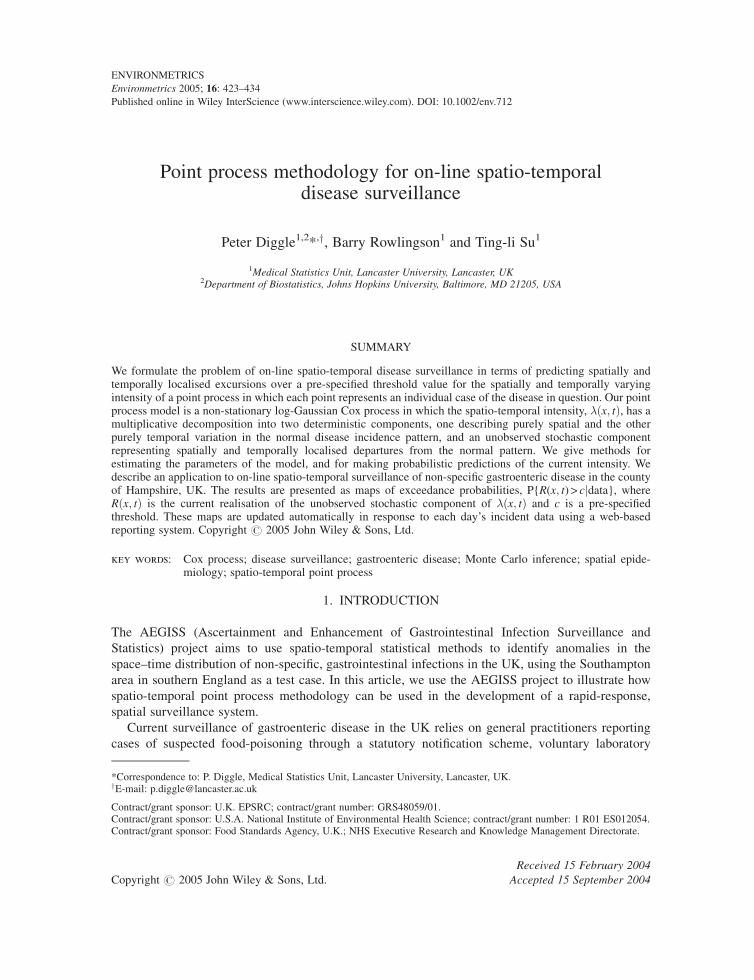
Figure 2 shows our estimated surface !!0!x" for the 2001 and 2002 NHS Direct data. This estimateuses the adaptive bandwidth prescription with h0 # 1:5 km in (4), resulting in local values of hiranging between 0.71 and 14.00.

4.2. Overall temporal variation

With the scalings adopted for !0!x" and for R!x; t", the function "0!t" represents the unconditionalexpectation of the number of cases on day t. We therefore estimate "0!t" by a standard Poisson

Figure 1. Summary results from simulation study to compare performance of adaptive and fixed bandwidth kernel estimators,

for different values of the Gaussian process parameters #2 and %. The plotted lines show point estimates (solid line) and

95 per cent confidence limits (dashed lines) for the ratio of minimum integrated squared errors achievable by adaptive and fixed

bandwidth estimators



log-linear regression model; note that the overdispersion induced by the stochastic component R!x; t"does not affect the consistency of point estimates derived from the Poisson model, but does invalidatethe nominal standard errors obtained under the Poisson assumption.

The empirical pattern of daily incident counts shows strong day-of-week effects, with excessnumbers especially at weekends when more traditional sources of medical advice are less accessible.Time-of-year effects are also apparent, with higher incidence in the spring and autumn. Finally, thereis an impression of an overall rising trend over time, which is likely to be due at least in part toprogressive uptake of the NHS Direct service during its early years of operation. To take account of allof these effects, we fitted the model

log"0!t" # 'd!t" & (1 cos!!t" & )1 sin!!t" & (2 cos!2!t" & )2 sin!2!t" & *t !6"

where ! # 2&=365, corresponding to annual periodicity in incidence rates. Point estimates for theday-of-week effects in the regression model (6) are ''d # 2:24; 1:92; 1:76; 1:82; 1:76; 1:78, 2.12, whered # 1 corresponds to Sunday, and so on. Point estimates of the harmonic regression parameters are((1 # $0:120, ))1 # $0:083, ((2 # $0:013 and ))2 # 0:054, whilst the estimate of the slope parameterfor the overall trend is ** # 0:00074. Figure 3 compares the fitted regression curve with observedcounts, averaged over successive one-week intervals to eliminate day-of-week effects.

4.3. Spatial and temporal dependence

To estimate parameters of S!x; t" we use the moment-based methods of Brix and Diggle (2001), whichoperate by matching empirical and theoretical descriptors of the spatial and temporal covariancestructure of the point process model. For the current analysis, we assumed a separable correlation

Figure 2. Kernel estimator for the overall spatial variation in reporting rates, !!0!x", based on NHS Direct data from the countyof Hampshire



structure in which $!u; v" # $x!u"$t!v". For the spatial component we used an exponential correlationfunction, $x!u" # exp!$juj=%". The corresponding spatial pair correlation function is g!u" #expf#2exp!$juj=%"g. We estimate #2 and % to minimize the criterion

!u0

0

'flog gg!u"g$ flog g!u"g(2du !7"

where u0 # 2 km and gg!u" is a non-parametric estimate of the pair correlation function. We use a time-averaged kernel estimator with Epanecnikov kernel function and bandwidth h # 0:2; hence

gg!u" # 1

2&uT jW j' (XT

t#1

Xn

i#1

X

i6#j

Kh!u$ k xi $ xj k"w!xi; xj"!t!xi"!t!xj"

!8"

In (8), each of the summations over i 6# j refers to pairs of events occurring on the same day, t, T is thestudy period, W the study area, Kh!u" # 0:75h$1!1$ u2=h2" when $h ) u ) h and zero otherwise,w!*" is Ripley’s (1977) edge correction, and !t!x" # !0!x""0!t" is the unconditional spatio-temporalintensity. The validity of this estimator relies on our assumption that the spatio-temporal covariancestructure is separable.

Figure 4(a) shows a good fit of the fitted parametric model for log g!u" to the non-parametricestimate log gg!u" defined by (8). The estimated parameter values are ##2 # 8:85 and %% # 0:19 km.

For the temporal correlation structure of S!x; t", we again assume an exponential form,$t!v" # exp!$jvj=+", and estimate + by matching empirical and theoretical temporal covariances of

Figure 3. Observed counts of reported cases per day, averaged over successive weekly periods (solid dots), compared with the

fitted harmonic regression model of daily incidence (solid line)



the observed numbers of incident cases per day, Nt say. For our model, the time variation in "0!t"makes the covariance structure of Nt non-stationary. We obtain

Cov!Nt;Nt$v" # "0!t"1!v # 0" & f"0!t""0!t $ v"g

+!

W

!

W

!0!x1"!0!x2"exp'#2exp!$v=+"exp!$u=%"(dx1dx2 $ 1

" #!9"

Note that the expression for Cov!Nt;Nt$v" given by Brix and Diggle (2001) is incorrect. Ourestimation criterion for + is

Xv0

v#1

Xn

t#v&1

fCC!t; v" $ C!t; v; +"g2

where v0 # 14 days and C!t; v; +" # Cov!Nt;Nt$v" as defined in (9). CC!t; v" is the empiricalautocovariance function, which is defined as

CC!t; v" # NtNt$v $ ""0!t"""0!t $ v"

Figure 4(b) compares the empirical autocovariance function of the time series of daily incident casesNt with ‘fitted’ covariance functions obtained by averaging the values of C!t; v; ++" and CC!t; v" overtime, t, for each time lag, v. The estimated value of the temporal correlation parameter is ++ # 2:0 days.

Figure 4. (a) Non-parametric (solid line) and fitted parametric (dashed line) log-pair correlation functions for the NHS Direct

data. (b) Empirical (dashed line) and fitted (solid line) autocovariance functions for the NHS Direct data. See text for detailed

explanation



5. SPATIO-TEMPORAL PREDICTION

To solve the prediction problem of interest, namely the identification of spatially and temporallylocalized occurrences of unusually high incidence, we first need to generate a sample from thepredictive distribution of the surface S!x; t", and hence R!x; t", conditional on the observed spatio-temporal pattern of incident cases up to and including time t. In practice, we do this on a fine grid oflocations xk; k # 1; . . . ;m, to cover the study region. As noted earlier, we also ignore uncertainty in theestimated values of the model parameters, on the grounds that, in this application, estimationuncertainty is negligible by comparison with prediction uncertainty. Having generated our sample,for each grid-point xk and a declared intervention threshold c, we approximate the predictiveprobability, p!xk; t; c" # PfR!xk; t" > cjdatag, by the observed proportion of sampled values R!xk; t"which exceed c. We then plot these approximate exceedance probabilities as a colour-coded map, inwhich the colour scale is chosen so as to highlight only sub-regions where p!x; t; c" is close to 1.

Following Brix and Diggle (2001), we use a Metropolis-adjusted Langevin algorithm (MALA) togenerate samples from the predictive distribution of the current surface S!x; t". Specifically, if Stdenotes the vector with elements S!xk; t"; k # 1; . . . ;m, and N t denotes the locations and times of allreported cases up to and including time t, the MALA generates samples from the conditionaldistribution of St given N t.

Although the process St is Markov in time, N t is not, and the predictive distribution of S!x; t"strictly depends on the complete history of N t. In practice, events from the remote past have avanishing influence on the predictive distribution of S!x; t". To avoid storing infeasible amounts ofhistorical data, Brix and Diggle (2001) applied a 5-day cut-off, determined experimentally as the pointbeyond which retention of historical data had essentially no effect on the predictive distribution. Theappropriate choice of cut-off will be application-specific, depending on the abundance of the data andthe pattern of temporal correlation. In principle, a straightforward modification of the algorithm can beused to generate samples from the predictive distribution of S!x; t & u" for any lead-time u. However,because of the short-range nature of the estimated temporal correlation, in our application forwardprojections rapidly become uninformative as the lead-time increases.

In our implementation of the MALA algorithm, we adjusted the variance of the proposaldistribution to achieve an acceptance rate of around 0.57, as recommended in Roberts and Rosenthal(1998), and used block-upating to sample from the predictive distribution of S!x; t" on each day, t, anda 256 by 256 grid of locations, x. Each day’s predictive probabilities were computed as empiricalproportions from a segment of 10 000 consecutive iterations. For a detailed description of the MALAalgorithm, see Møller and Waagepetersen (2004).

For prediction using the NHS Direct data we fixed all of the model parameters at their estimatedvalues, with the exception of the temporal trend parameter * in (6). This parameter was included in themodel to allow for progressive uptake in the use of the NHS Direct service. On the assumption that theoverall level of use has now stabilized, we chose to extrapolate the linear trend at a constant level **t0,where t0 corresponds to 31 December 2002. However, and as discussed in Section 6 below, theaccuracy of this and other parametric assumptions can and should be reviewed periodically as dataaccumulate over time.

An integral part of the AEGISS project is to develop a web-based reporting system in whichanalyses are updated whenever new incident data are obtained. Each day, a program running inLancaster checks for the arrival of new data. Whenever five consecutive days of data are identifed,these data are then passed to another program, which runs the spatial prediction algorithm. Outputsfrom the prediction algorithm in the form of maps of the exceedance probability surfaces p!x; t; c" for



each of a set of values of c are then passed back to a web-site. The actual analyses of the data arecarried out using C programs with an interface to the R system (http://www.r-project.org/).

The threshold values used on the web-site are currently c # 2, 4 or 8. However, it would bepreferable to relate these to the estimated parameters of the fitted model. Under our assumed model,the p-quantile of R!x; t" is c # expf$0:5#2 & #"$1!p"g. Setting #2 at its estimated value 8.85 wouldgive threshold values c # 0:54, 1.60 and 12.13, corresponding to p # 0:9, 0.95 and 0.99, respectively.

Figure 5 shows a static example of the surface p!x; t; c" for t corresponding to 6 March 2003, andthreshold value c # 4. The map suggests three possible anomalies near the south-west, south-east andnorth-east boundaries of the study region. In practice, it is more useful to track the evolution ofp!x; t; c" over successive days. An anomaly which appears one day and disappears the next is likely tobe dismissed by a public health practitioner as a false positive, whereas one which persists over a fewdays, or at higher thresholds c, should prompt an intervention of some kind. The web-site http://aegissdev.lancs.ac.uk:8080/Demo/ contains a record of daily updates over a three-monthperiod, which can be examined interactively. Simple click operations allow the user to step forwardand backward in time, and through the available values of c. These are currently set as c # 2, 4 and 8.

6. DISCUSSION

Point process modelling has the advantage that it does not impose artificially discrete spatial ortemporal units on the underlying risk surface. Specifically, the scales of stochastic dependence in spaceand in time are determined by the data, and these estimated scales are then reflected in the amounts ofspatial and temporal smoothing that are applied in constructing the predicted risk surfaces.

A possible objection to our particular model is that the Cox process is not a model for infectiousdisease. However, because of the duality between spatial clustering and spatial heterogeneity of risknoted by Bartlett (1964), our inhomogeneous Cox process model can describe clustered patterns ofincidence empirically by ascribing local spatio-temporal concentrations of cases to peaks in the

Figure 5. Posterior exceedance probabilities, p!x; t; c" # P'R!x; t" > cjN t(, for t corresponding to 6 March 2003 and c # 4



stochastic process R!x; t", after adjusting for overall spatial and temporal trends through thedeterministic functions !0!x" and "0!t". It is partly for this reason that we suggest using the term‘anomaly’ rather than ‘outbreak’ to describe our findings, as we recognize that some anomalies willprove to be artefactual. In other words, we aim only to provide early indications of possible outbreaks,rather than definitive evidence that an outbreak has occurred.

Another possible concern is that our approach necessarily assumes that the residential location ofeach case is substantively relevant. In practice an individual’s exposure to risk is determined by acomplex combination of their residential, working and leisure locations and activities.

In specifying the spatial–temporal covariance function for S!s; t", it is computationally advanta-geous to use a separable structure and the exponential form for the temporal correlation component,which makes the process Markovian in time. There is no corresponding advantage to using anyparticular form for the spatial correlation component, although coincidentally the exponential againprovides a reasonable fit to the data.

Our current methods of parameter estimation, especially with regard to the spatial and temporalcovariance parameters, are very ad hoc. We are adapting the methods described in Benes et al. (2002)and Møller and Waagepetersen (2004) to obtain maximum likelihood estimators of our modelparameters. We are also conducting a simulation study of the area-wide sensitivity and specificityof the prediction algorithm by superimposing on the real data synthetic outbreaks of varying size andspatio-temporal extent.

The work reported here used data on cases reported up to the end of 2002. Examination of datasubsequently obtained for 2003 illustrates the need for periodic review of the fitted model parameters.For example, Figure 6 shows an extrapolation of Figure 3, in which the model for the mean dailyincidence, ""0!t", fitted from 2001 and 2002 data, has been projected forward in time and compared with

Figure 6. Observed counts of reported cases per day, averaged over successiveweekly periods, for the years 2001 to 2003 (solid

dots) compared with the harmonic regression model of daily incidence fitted to data from 2001 and 2002 only, extrapolatedthrough 2003 using a continuation of the fitted linear term (solid line) and with the linear term extrapolated at constant level

corresponding to 31 December 2002 (dashed line)



the actual 2003 data. The two projections correspond to continuation of the linear increase through2003 and extrapolation of the linear term at a constant level. The actual 2003 data show the anticipatedspring peak in incidence, but thereafter the incidence declines sharply by comparison with either of theextrapolated curves. To address this, we are investigating the use of a stochastic term in place of thedeterministic linear trend component *t on the right-hand side of (6), as in West and Harrison (1997).

In conclusion, we have illustrated how spatial statistical methods can help to develop on-linesurveillance systems for common diseases. The spatial statistical analyses reported here are intendedto supplement, rather than to replace, existing protocols. Their aim is to identify, as quickly aspossible, statistical anomalies in the space–time pattern of incident cases, which would then befollowed up by other means. In some cases, the anomalies will be transient features of no particularpublic health significance. In others, the statistical early warning should help to ensure timelyintervention to minimize the public health consequences—for example, when follow-up of cases in anarea with a significantly elevated risk reveals exposure to a common risk factor or infection with acommon pathogen.

ACKNOWLEDGEMENTS

This work was supported by the UK Engineering and Physical Sciences Research Council through the award of aSenior Fellowship to Peter Diggle (Grant number GR/S48059/01) and by the U.S.A. National Institute ofEnvironmental Health Science through Grant number 1 R01 ES012054, Statistical Methods for EnvironmentalEpidemiology.Project AEGISS is supported by a grant from the Food Standards Agency, U.K., and from the National Health

Service Executive Research and Knowledge Management Directorate. We also thank NHS Direct, Hampshire andIsle of Wight, participating general practices and their staff, and collaborating laboratories for their input toAEGISS.

REFERENCES

Bartlett MS. 1964. The spectral analysis of two-dimensional point processes. Biometrika 51: 299–311.Benes V, Bodlak K, Møller J, Waagepetersen R. 2002. Bayesian analysis of log Gaussian processes for disease mapping.Research Report No 3, February 2002, Centre for Mathematical Physics and Statistics, University of Aarhus, Denmark.

Berman M, Diggle P. 1989. Estimating weighted integrals of the second-order intensity of a spatial point process. Journal of theRoyal Statistical Society B 51: 81–92.

Brix A, Diggle PJ. 2001. Spatiotemporal prediction for log-Gaussian Cox processes. Journal of the Royal Statistical Society, B63: 823–841.

Cooper DL, Smith GE, O’Brien SJ, Hollyoak VA, Baker M. 2003. What can analysis of calls to NHS Direct tell us about theepidemiology of gastrointestinal infections in the community? Journal of Infection 46: 101–105.

Cox DR. 1955. Some statistical methods related with series of events (with Discussion). Journal of the Royal Statistical Society,Series B 17: 129–157.

Diggle PJ. 1985. A kernel method for smoothing point process data. Applied Statistics 34: 138–147.Diggle PJ, Ribeiro PJ, Christensen O. 2003. An introduction to model-based geostatistics. In Spatial Statistics andComputational Methods: Lecture Notes in Statistics, Vol. 173, Møller J (ed.). Springer: New York; 43–86.

Diggle PJ, Knorr-Held L, Rowlingson B, Su T, Hawtin P, Bryant T. 2003. On-line monitoring of public health surveillance data.In Monitoring the Health of Populations: Statistical Principles and Methods for Public Health Surveillance, Brookmeyer R,Stroup DF (eds). Oxford University Press: Oxford; 233–266.

Hall P, Hu TC, Marron JS. 1995. Improved variable window kernel estimates of probability density. The Annals of Statistics23(1): 1–10.

Møller J, Waagepetersen R. 2004. Statistical Inference and Simulation for Spatial Point Processes. Chapman & Hall: London.Møller J, Syversveen A, Waagepetersen R. 1998. Log Gaussian Cox processes. Scandinavian Journal of Statistics 25: 451–482.Ripley BD. 1977. Modelling spatial patterns (with discussion). Journal of the Royal Statistical Society B 39: 172–212.Roberts GO, Rosenthal JS. 1998. Optimal scaling of discrete approximations to Langevin diffusions. Journal of the RoyalStatistical Society, Series B 60: 255–268.

Silverman BW. 1986. Density Estimation for Statistics and Data Analysis. Chapman & Hall: London.West M, Harrison J. 1997. Bayesian forecasting and dynamic models. In Spatial Statistics and Computational Methods: Secondedition. Springer: New York.



point process methodology for on-line spatio-temporal...

Documents