OECD Global Forum on International Investment OECD Investment Division www.oecd.org/investment/gfi-7

POLICIES TO ATTRACT FOREIGN DIRECT INVESTMENT: AN INDUSTRY-LEVEL ANALYSIS

C.Bellak, M.Leibrecht & R.Stehrer

Session 1.1: Investment policy

This paper was submitted in response to a call for papers conducted by the organisers of the OECD Global Forum on International Investment. It is distributed as part of the official conference documentation and serves as background material for the relevant sessions in the programme. The views contained within do not necessarily represent those of the OECD or its member governments.

2

Abstract

This paper analyzes policies to attract Foreign Direct Investment (FDI) based on a sample comprising the US plus six EU countries (US-plus-EU-6) and four Central and Eastern European Countries (CEEC-4). The analysis draws on industry-level data for 1995-2003. A Dynamic Panel Data approach is used to isolate important country- and industry-level determinants of FDI inward stock. The estimated baseline model derived is used to assess the scope for FDI attraction policies. The scope for FDI is defined as the difference between the FDI inward stock received by a country-industry-pair, as implied by the baseline model (“estimated FDI”), and the inward FDI stock which could be realized if a certain “best practice” policy were carried out (“potential” FDI). The results show how different policy variables contribute to closing the gap between estimated and potential FDI. The countries in our sample fall into two groups: In the CEEC-4 an increase of R&D expenditures in GDP would result in a substantial increase in FDI, while in the US-plus-EU-6 an improvement of their unit labor cost position, e.g. via increases in labor productivity, and improvements in their tax position would attract additional FDI.

Keywords: Economic Policy, Foreign Direct Investment, European Union, Industry-level Study, Location Decision

JEL codes: F21, H25, H71

* University of Economics and Business Administration Vienna, Department of Economics, Augasse 2-6, A-1090 Vienna, Austria

**The Vienna Institute for International Economic Studies (wiiw), Oppolzergasse 6. A-1010 Vienna, Austria, Corresponding author e-mail: christian.bellak@wu-wien.ac.at

Paper prepared within the “Forschungsschwerpunkt Internationale Wirtschaft (FIW), Arbeitspaket 2: Direktinvestitionen. We are grateful for financial support by the Bundesministerium für Wirtschaft und Arbeit, Vienna, Austria.

3

1. Introduction

Policies to attract Foreign Direct Investment (FDI) have become standard in most countries, irrespective of their level of development, geographical location or industrial structure. One of the most important policy questions is: (i) What should be done in order to attract inward FDI? This question asks which policy variables can be used to attract FDI in general. Here, a policy variable is defined as a determinant of FDI which can be directly influenced by governments (“policy makers”) in the short run.1 A related question is: (ii) How large is the scope for FDI in general and in certain industries in particular? The scope for FDI is defined as the amount of additional FDI, which could be attracted if FDI-relevant policy variables were improved towards an international “best practice policy”.

In this paper we address both of these questions with the aim of providing some insight to policy makers seeking promising areas of action and an efficient means of conducting FDI attraction policies. To this end, we isolate the economically and statistically most important determinants of inward FDI stock in the US and 6 EU member countries (US-plus-EU-6) as well as in four Central and Eastern European Countries2 (CEEC-4) over a time span of nine years (1995 - 2003) using industry-level data. In doing so, we place a particular focus on five policy variables: taxes, R&D expenditures, unit labor costs, the skill level of workers and the FDI-related institutional environment, which are continuously mentioned in the public discussion.

We proceed in two steps: (i) estimation of a baseline model using econometric methods for dynamic panel models and (ii) calculation of gaps between estimated and potential FDI inward stock based on the definition of “best practice policy” values of the included policy variables. The calculated gaps show which location factors should be addressed by policy makers to increase FDI inward stock in certain industries.

Despite an econometric analysis shows which variables impact economically and statistically significant on inward FDI stock it does not give an impresion which of the (policy) variables should be altered to attract FDI given a country's relative position with respect to the various policy measures, i.e. whether a country is below or above the "best practice policy” values. Put differently, an analysis based on the gap between estimated and potential FDI also shows which FDI attraction policies should be carried out by a particular country in a particular industry.

In relation to our approach, several studies have been carried out based on FDI data at the industry level. Resmini (2000) uses FDI flow data (i.e. FDI flows in US dollars in 10 CEECs in four subcategories of the manufacturing sector using the Pavitt classification; see Pavitt, 1984) over 1991-1995. Bénassy-Quéré et al. (2007a) use FDI stock data (i.e. capital expenditures by US majority-owned affiliates) in 18 EU members for eleven industries over 1994-2002. Yeaple (2003) analyzes the role of skill endowments for the structure of US outward FDI defined in terms of the sales of U.S. multinationals‟ majority-owned affiliates abroad based on the benchmark survey of 1994, covering 39 countries (no CEEC) and 50 manufacturing industries. Basically, these studies confirm the traditional determinants of FDI – foremost market-related and efficiency-related location factors. With respect to the first policy variable of main interest in this

1 Examples are taxes, R&D expenditures or the institutional environment. Factors that can only be influenced indirectly

or in the medium to long run might be called “intervention variables”. The inflation rate would be an example for such a variable.

2 The EU countries included are: Austria (AUT), Finland (FIN), France (FRA), Great Britain (GBR), the Netherlands

(NLD), Germany (GER), the Czech Republic (CZE), Hungary (HUN), Slovenia (SVN) and Slovakia (SVK).

4

paper (tax rates) these studies reveal that countries with a high corporate income tax rate receive less FDI (Yeaple 2003, p. 730, Table 1; Bénassy-Quéré et al. 2007, p. 37ff., Tables 1 and 2; whereas taxes are not included in Resmini 2000). The second policy variable of main interest in this paper, R&D expenditures in GDP, has not been included in the studies just mentioned. The third policy variable of main interest, the institutional environment, is reflected by a number of single indicators, but in general has not been given much emphasis in other studies using industry-level data. Yeaple (2003) uses an indicator reflecting a country‟s openness to FDI. His finding suggests that the effect of barriers to FDI is larger for vertical FDI (re-exporting) than for local market oriented FDI. Recently, Bénassy-Quéré et al. (2007b) focused on home and host country institutional determinants of FDI on the basis of a unique database which includes firm-level data on the institutional quality. Their findings suggest “that efforts towards raising the quality of institutions and making them converge towards those of source countries may help developing countries to receive more FDI. The orders of magnitude found in the paper are large, meaning that moving from a low level to a high level of institutional quality could have as much impact as suddenly becoming a neighbour of a source country.” (ibidem, p. 781) These and other findings suggest that including institutional determinants of FDI is indeed important in the empirical research of policy determinants.

Concerning the calculation of gaps among recent studies which include CEECs in an effort to estimate FDI potential, Demekas et al. (2007) and Resmini (2000) are particularly relevant. Demekas et al. (2007) use FDI stocks to derive the concept of potential FDI “… using the actual values of exogenous variables and the „best‟ values the policy variables can take.” (p. 378). The gap is defined as the level of FDI predicted by the model, which is based on the actual values of exogenous variables and potential FDI calculated using the “best practice policy” values of policy variables. Here, the “best” values are defined as the lowest or highest values of each location factor in the sample. The calculated gaps range from 2 to 83 percent, depending on the country in question. Demekas et al. (2007) point out that their effects should be interpreted as short run effects and that “… the government may have limited control over some policy variables in the short term.” (p. 379). One drawback of this study is, however, that it seems questionable that using minimum and maximum values as “best practice policy” values will reflect likely policy scenarios in a sample of heterogenous countries, especially in the short run. A change of policy variables by a substantial amount can usually only be achieved in the medium to long run.

Resmini (2000) defines the gap as the ratio of actual FDI flows to the fitted values from her baseline specification and distinguishes several types of industries in CEECs in 1995 (according to the Pavitt taxonomy). The estimated gaps range from 43 percent for high-tech sectors to 88 percent in traditional sectors (see Table 5 in Resmini 2000 for details). A drawback of this study is that the fitted values from her benchmark specification are used to represent FDI “potential”. Yet, from a statistical point of view, the gap between this potential FDI and actual FDI values reflects that part of the model which is not explained by the variables included in the model. Thus, this gap cannot be closed by changing the policy variables included in the model. Therefore, we essentially follow the approach suggested in Demekas et al. (2007) using two alternative specifications of the “best practice policy” values.

The paper contributes to the literature in several ways. First, FDI inward stocks at the industry level, which are a reasonable proxy for the distribution of productive capital across countries and industries (e.g. Blonigen et al. 2003), are used as the dependent variable. Thereby, the dynamic nature of the data generation process underlying the FDI stock data is modeled. Second, gaps between estimated and potential FDI inward stocks are calculated for the US-plus-EU-6 and CEEC-4, separated by policy variables as well as by countries and by industries to reveal which policy variables policy makers should use to increase FDI inward stock in certain industries.

5

)1(loglog ,,3,21,1 tijijttijtitijijt ZbXbFDIbFDI

Third, another novelty of this paper is the inclusion of variables at an industry level – such as the share of low-skilled workers or unit labor costs based on hours worked – which have only recently been made available.3

The paper is structured as follows: Section 2 presents the empirical model on which our analysis is based and in section 3 we give information concerning methodological aspects. The results are shown and discussed in section 4. Section 5 summarizes and concludes.

2. The empirical model

In order to isolate the relevant determinants of the FDI location decision of a Multinational Enterprise (MNE) we assume that, out of a number of k potential locations (countries), a firm will

decide to invest where after-tax profits (net ) are higher compared to alternative locations:

)......,max(_ 1

net

k

netlocationFDI (see Devereux and Griffith 1998: 344 and 349). The crucial

question in deriving the empirical model is, therefore, which location factors impact on the after-tax profit of an investment. Moreover, as the FDI inward stock usually shows high serial dependence and to neglect this serial correlation might lead to a dynamically mis-specified empirical model, our empirical specification is derived from a dynamic panel data framework. Specifically, variants of the following equation (1) will be estimated using the estimator recently proposed by Blundell and Bond (1998)4:

Thus, ijtFDIlog is the logarithm of the inward FDI stock of country i, sector j in year t. itX are

location factors which vary over countries and over time and ijtZ are variables which vary over

time and over country-industry pairs. t are time dummies (TD), ij are country-industry-pair-

specific fixed effects, which capture the impact of time-invariant country, industry and country-

industry factors and ijt is the remainder error term.

Which factors have an impact on the after-tax profit of an investment and thus need to be

included in tiX , and tijZ , ? Generally, gross profits are a function of revenues and production

costs, which crucially depend on the optimal level of output. Put differently, inter alia, gross profits depend on the determinants of marginal costs and marginal revenues. These determinants include factors like the market size, gross wages, labor productivity or the availability of capital (Devereux and Griffith 1998: 343; Clausing and Dorobantu 2005: 87). Furthermore, gross profits also depend on any fixed costs incurred by investing in a foreign location. For example, a country‟s political and macroeconomic risk level may generate transaction costs that have to be covered independently of any effective production activity. Net or after-tax profits additionally depend on the taxation of profits in the host country.

We separate the location factors into market- and efficiency-related variables (e.g. Markusen and Maskus 2002), with the first mainly influencing marginal revenues and the latter influencing

3 Specifically, data from the EU-KLEMS project are used.

4 Specifically, the xtabond2 Stata program of D. Roodman (see e.g. Roodman 2007a) is used.

6

marginal and fixed costs. The variables considered are the market potential ( itPot ) and the GDP

per capita ( itGDPcap ) of a host country i, unit labor costs ( tijUlc , ), the share of low-skilled hours

worked ( tijlsH ,_ ), the average effective tax rates on corporate profits ( itEatr ), private and public

R&D expenditures as percent of GDP ( itGerd ), the political risk level ( itRisk ) and the

macroeconomic risk level ( itInflation ). Moreover we use the level of legal barriers to FDI

( itFreefdi ), which can be considered as a precondition for market- and efficiency-related FDI to

take place (cf. Table 1).

Table 1: Classification of Location factors

Group Country-level variability Country-industry-level variability

Market related variables

Market potential, GDP per capita in PPP, legal barriers to FDI

lagged FDI inward stock

Efficiency related variables

Macroeconomic risk, GDP per capita in PPP, political risk, taxes, R&D

expenditures, legal barriers to FDI

Unit labor costs, share of low-skilled hours worked

Thus, itEatr , itGerd , itFreefdi , tijUlc , and tijlsH ,_ are “policy variables”, as they can be directly

influenced by policy makers in the short run, for example via changes in tax or competition law, public R&D expenditures, bilateral investment treaties, wage subsidies, etc.. At the same time

itRisk , itInflation , itPot and itGDPcap are “intervention variables” which can only indirectly be

influenced by policy makers and/or only in the medium to long run.

We expect itPot to have a positive impact on FDI as this variable captures market size. An

increase in market size, ceteris paribus, should have a positive impact on marginal revenues and

hence the profits of a firm. The sign of the coefficient of itGDPcap is ambiguous a priori (e.g.

Bénassy-Quéré et al. 2007b), pointing toward its role as a “catch-all” variable: On the one hand this variable captures the capital abundance of a host country and, as more capital abundant countries should receive less capital, a negative sign should be expected (e.g. Egger and

Pfaffermayr 2004). Moreover, itGDPcap might represent effects of wage costs on the marginal

costs of an FDI (e.g. Mutti and Grubert 2004), again implying a negatively signed coefficient. On

the other hand, itGDPcap captures positive effects on an FDI‟s profit level via a favorable

infrastructure endowment (e.g. Mutti 2004), high demand and labor productivity (e.g. Mutti and Grubert 2004), as well as better institutions (e.g. Bénassy-Quéré et al. 2007b). Thus, in principle, the host country‟s GDP per capita could be substituted by these underlying variables. As we do

not have valid proxies for each of these variables we have included itGDPcap in the empirical

model.

7

Unit labour costs tijUlc , are used to capture the impact of labor productivity and wage rates on

FDI. An increase in unit labour costs, ceteris paribus, increases marginal costs, and we therefore

expect a negatively signed coefficient. The share of low-skilled workers, tijlsH ,_ , is used as a

proxy for the skill level. We opt for the share of low-skilled workers as the data seem to be more reliable than those on high-skilled workers, which to a large extent also reflect country specificities in the educational system that can blur the distinction between medium and high-skilled workers. Further, in the manufacturing sector in particular, the medium educated workers (including technicians) are important for productivity performance, among other factors. The sign of the coefficient depends on the underlying motive for FDI, i.e. whether it is efficiency-seeking or

market-seeking FDI. In the first case, an increase in tijlsH ,_ could lead to an increase of

(vertical) FDI originating in high skill countries/industries as MNEs exploit differences in factor endowments. In the second case, the sign should be negative, as firms duplicate plants (export substitution) and most FDI originates in high income, high skill countries (e.g. Barba Navaretti and Venables 2004, chapter 2). Thus, the sign is indeterminate a priori.

We use the change in producer prices, itInflation , as a proxy for macroeconomic risk, as a high

inflation rate implies macroeconomic uncertainty. Larger uncertainty may translate into higher fixed costs of production, for example due to larger efforts to insure against risks of various forms or due to larger transaction costs in establishing and enforcing contracts. Thus, we expect an

increase in itInflation to lead to a decrease in FDI. The same reasoning applies to the political

risk level of a country itRisk . Yet, due to the particular definition of the measure of itRisk , we

expect a positive coefficient.

The itFreefdi variable is intended to capture legal barriers to inward FDI. In particular, this

variable incorporates restrictions on FDI which limit the inflow of capital and thus hamper economic freedom. By contrast, little or no restriction of foreign investment enhances economic freedom because foreign investment provides funds for economic expansion. For this factor, the more restrictions countries impose on foreign investment, the lower their level of economic freedom will be and the higher will be their score. Thus, a negative sign is expected for this variable.

itEatr is used as a proxy for the corporate income tax burden, as the after-tax profit is directly

determined by the average tax rate (see Devereux and Griffith 1998: 344). Moreover, the itEatr

is calculated as the weighted average of an adjusted statutory tax rate on corporate income and the effective marginal tax rate (see Devereux and Griffith 1999 for details). Thus, it combines the effects of corporate taxes on FDI with very high levels of profitability and effects on marginal investments which determine the volume of an existing capital stock. A negatively signed

coefficient is expected here, as a higher itEatr implies a lower level of after-tax profits.

One of the aims of the EU “Lisbon-strategy” is for the EU to become a competitive and dynamic science-based economic area by 2010, where an increase in the member states‟ R&D ratio acts as an important policy instrument (e.g. Commission of the European Communities 2004,

COM(2004) 29 final/2). In addition to this, an increase in itGerd , for example via an increase in

its public component, should also have a positive impact on FDI, as a country‟s R&D level can be considered a type of public good that makes firms more productive without causing additional

8

costs. That is, firms may gain from positive knowledge spill-over effects which contribute to a higher profit level from their investment.

Finally, note that the lagged FDI inward stock, 1, tijFDI , also conveys some substantive meaning

in addition to its role in capturing inertia. A high FDI stock in the past in a particular industry can be seen as a signal to potential foreign investors (“demonstration effect”; e.g. Barry et al. 2004). If firms seek each other‟s proximity to reap industry-specific spillovers, making them more productive without causing additional costs, a high past FDI stock should also have a positive impact on the current FDI stock.5

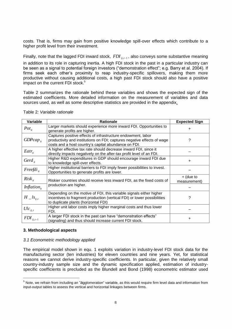
Table 2 summarizes the rationale behind these variables and shows the expected sign of the estimated coefficients. More detailed information on the measurement of variables and data sources used, as well as some descriptive statistics are provided in the appendix.

Table 2: Variable rationale

Variable Rationale Expected Sign

itPot Larger markets should experience more inward FDI. Opportunities to generate profits are higher.

+

itGDPcap Captures positive effects of infrastructure endowment, labor productivity and institutions on FDI; captures negative effects of wage costs and a host country‟s capital abundance on FDI.

?

itEatr A higher effective tax rate should decrease inward FDI, since it directly impacts negatively on the after-tax profit level of an FDI.

–

itGerd Higher R&D expenditures in GDP should encourage inward FDI due to knowledge spill-over effects.

+

itFreefdi Higher institutional barriers to FDI imply fewer possibilities to invest. Opportunities to generate profits are lower.

–

itRisk Riskier countries should receive less inward FDI, as the fixed costs of production are higher.

+ (due to measurement)

itInflation –

tijlsH ,_ Depending on the motive of FDI, this variable signals either higher incentives to fragment production (vertical FDI) or lower possibilities to duplicate plants (horizontal FDI)

?

tijUlc , Higher unit labor costs imply higher marginal costs and thus lower FDI.

–

1, tijFDI

A larger FDI stock in the past can have “demonstration effects” (signaling) and thus should increase current FDI stock.

+

3. Methodological aspects

3.1 Econometric methodology applied

The empirical model shown in equ. 1 exploits variation in industry-level FDI stock data for the manufacturing sector (ten industries) for eleven countries and nine years. Yet, for statistical reasons we cannot derive industry-specific coefficients. In particular, given the relatively small country-industry sample size and the dynamic specification applied, estimation of industry-specific coefficients is precluded as the Blundell and Bond (1998) econometric estimator used

5 Note, we refrain from including an ”agglomeration“ variable, as this would require firm level data and information from

input-output tables to assess the vertical and horizontal linkages between firms.

9

necessitates a relatively large cross-section (i.e. in our case many country-industry pairs). For the total maufacturing sector the number of pairs (about 105; cf. Table 3) is sufficient. Yet for the calculation of industry-specific coefficients the number would be too low.

We apply a general-to-specific-approach as we start with the most general model (including all location factors shown in Table 1), the full model, and test down until only statistically significant variables remain (at the 10 percent significance level), which lead us to the baseline model. This procedure is expected to reduce the possibility of an omitted variable bias and it also shows the robustness of our results to the inclusion and exclusion of location factors. Thereby, variables measured in Euros are used in logs in addition to the FDI stock. All other variables are used in levels.

One advantage of using the Blundell and Bond (1998) estimator is that, if there is high inertia in the dependent variable, it avoids biased estimates in finite samples due to a “weak instrument” problem (see Arellano 2003: 115 and Bond 2002: 20 on this issue) and it results in an increase in efficiency, especially if the time dimension is short. This improved efficiency is the result of an exploitation of additional moment conditions. The validity of these conditions, however, requires mean stationarity of the initial conditions. If mean stationarity is not valid, the Blundell and Bond estimator will lead to inconsistent estimates (“initial condition bias”; Arellano 2003: 112). Thus, it is crucial to test the validity of this assumption.

Another important advantage of the Blundell and Bond (1998) estimator is that it allows us to specify the type of exogeneity (i.e. strictly exogenous, predetermined or endogenous) of the right hand variables. With the exception of year dummies, all variables are considered either

predetermined (i.e. itEatr , 1, tijFDI , itFreefdi ) or endogenous to FDI (all other variables). The

endogeneity assumption for these variables is justified as it is plausible for FDI to have an immediate impact on GDP, labor costs, the skill level and the risk level of a country and industry

respectively. For itEatr and itFreefdi it is plausible for FDI to have an impact on the future

values of these variables only, rendering them exogenous or predetermined. This grouping of variables has an impact on the instruments used, as the lag structure of the instruments is adjusted accordingly.

To avoid the problems of biased estimates (“overfitting”) and weak Hansen and Difference-in-Sargan tests caused by too many instruments, we restrict the latter. In particular, instead of using all possible instruments for each available time period, we “collapse” the matrix of instruments.6 Collapsing actually implies that coefficients on instruments are forced to be equal. This gives us a smaller set of instruments without a loss of lags and therefore also information (see Roodman 2007b: 18 for details). Year dummies are considered strictly exogenous and included as instruments for the level equation only to ensure a correct number of degrees of freedom (Bond 2002). Throughout the estimation, the asymptotically efficient two-step GMM estimator with corrected standard errors (“Windmeijer-correction”) is applied.

We generally conduct two-sided tests. However, to test the significance of the coefficients of those location factors for which the expected sign is a priori unambiguous we apply one-sided tests. The alternative hypothesis in these cases is according to the expected sign (cf. Table 2).

3.2 Calculation of estimated and potential FDI

6 Option collapse in xtabond2 is used.

10

To calculate the potential FDI in a first step, the “best practice policy” is determined for the policy

variables included in our analysis (that is itEatr , itGerd and itFreefdi as well as tijUlc , and

tijlsH ,_ the latter two being industry-specific variables) and for the most recent year (i.e. 2003).

In our case the “best practice policy” is assumed to be either the sample mean (replacing the mean by the median does not change the results much) or the minimum or maximum value in the sample considered (cf. Table 4).

In a second step, the “best practice policy” value is substituted for the actual value of the policy variables if the actual value can be improved.7 In a third step, the estimated coefficients from the baseline model are used to predict the value of FDI inward stock if the “best practice policy” value is realized, keeping everything else equal, including the assumption that other countries have not improved their location factors. This predicted value is defined as the potential FDI stock (P). Fourth, the predicted value of the FDI stock as given from our baseline model is calculated. This yields the “estimated” FDI inward stock (E). The predicted FDI from the baseline model is used instead of actual FDI value in order to establish a common benchmark (same data generation process) for all country-industry pairs against which changes in policy variables are evaluated. Moreover, using predicted FDI allows for a direct comparison of the effects of changes in a policy factor on attracted FDI across country-industry-pairs, as all other conditions (including the coefficients of the data generation process) remain constant. Fifth, the quota (Q) of the estimated (E) and the potential stock (P) is calculated, i.e. Q = (E/P*100). Thus, if the “best practice policy” were implemented, the potential percentage point change in FDI stock would be 100-Q.

We calculate two types of gaps: the first on a country and industry basis under the assumption that all policy variables are set jointly at their “best practice policy” values (“total gap”; cf. Figures 1a and 1b). The second type of gap is calculated for each of the policy variables separately, i.e. with all other policy variables remaining at their actual values (“variable specific gaps”; cf. Figures 2a and 2b.8

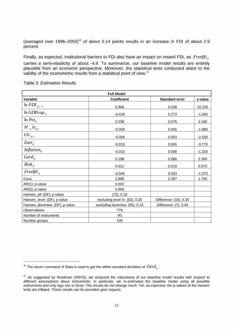
4. Results

4.1 Econometric analysis

Table 3 presents the results of our econometric analysis with the upper part showing the “full model” results which contain all variables shown in Table 1. Only the short-run coefficients are shown, as we are interested in the impact of policy changes on FDI in the short run like Demekas et al. (2007).

Despite carrying the expected signs, itRisk and itInflation fall short of statistical significance

even when one-sided tests are applied. Political risk, in particular, is not among the relevant determinants of FDI. This result is plausible as the countries included are among the most

developed market economies with a high level of political stability. Excluding itRisk first, as it has

7 For example, for itGerd the “best practice policy” value (maximum value) is the value of FIN (3.43). This value is

substituted for the actual values of each country-industry pair.

8 Note that the sum of the specific gaps is not equal to the total gap. Indeed, the sum of individual gaps has to be

higher as the denominator of each individual gap is smaller in value than that of the total gap.

11

the lowest z-value, provides us with our baseline model.9 Note that the exclusion of itRisk has

only a minor impact on the estimated coefficients of the other variables. Only itInflation becomes

significant when applying a one-sided test, with a semi-elasticity of about -1. This favors a weak negative impact of a higher macroeconomic risk level on FDI.

As expected, the lagged FDI inward stock has a substantially positive impact on the current FDI stock. Indeed, interpreting the z-value as a rough guide for the relative importance of the various variables as location factors, this signals that this variable is the most important determinant of

current inward FDI stock. The negative sign of itGDPcapln signals that more capital abundant

countries receive less FDI.

The coefficient of itPotln , although it carries the expected sign, is rather low. Yet one should

bear in mind that we are explaining FDI inward stocks at the industry level, whereas itPotln is

measured at the country-level. As countries with small market size may receive substantial parts of total world FDI in certain industries while receiving relatively few FDI in total, this low

coefficient of itPotln is plausible.

The semi-elasticities of tijlsH ,_ and tijUlc , are -0.8 and -0.6, respectively. The negative sign of

the tijlsH ,_ coefficient suggests that, in the countries and industries included, FDI is of a

predominantely horizontal nature. This result is in line with many other studies (e.g. Markusen

and Maskus 2002). A one percentage point decrease in tijUlc , increases FDI by about 0.6

percent. This rather low semi-elasticity might be a further indication that most FDI is horizontal FDI, as market-seeking FDI is probably not as sensitive to labor costs as efficiency-seeking FDI.

A decrease in the itEatr by one percentage point increases FDI by about 1.9 percent according

to the baseline model. This negative impact of the itEatr on FDI is in line with many other

studies, notably the meta-analysis carried out by DeMooij and Ederveen (2005). DeMooij and Ederveen (2005) find a median tax-rate elasticity of FDI of about -3. Moreover, Stöwhase (2005) analyzes the tax responsiveness of FDI flows into several EU countries on a sectoral level. Using effective tax rates to measure tax incentives, Stöwhase (2005) is able to show that the tax sensitivity of FDI crucially depends on the economic sector. While investment in the primary sector is driven by factors other than tax incentives, investment in the secondary and the tertiary sector is deterred by high tax rates.

An increase in the itGerd by one percentage point leads to an increase in the FDI inward stock

by about 21 percent. At first sight, this value seems rather high. Yet one must consider that a one percentage point change marks a pronounced change in this variable, which is measured as

percent of GDP. Evaluating the impact of itGerd at the within country standard deviation

9 Note that itRisk is kept as an instrument as this is strongly suggested by the Hansen-test for the validity of

overidentifying restrictions. Using itRisk as an external instrument is justified, as on the one hand it is probably

correlated with some of the right hand variables and on the other hand – given the results from the full model – it is not correlated with the error term.

12

(averaged over 1996–2003)10 of about 0.14 points results in an increase in FDI of about 2.9 percent.

Finally, as expected, institutional barriers to FDI also have an impact on inward FDI, as itFreefdi

carries a semi-elasticity of about -4.9. To summarize, our baseline model results are entirely plausible from an economic perspective. Moreover, the statistical tests conducted attest to the validity of the econometric results from a statistical point of view.11

Table 3: Estimation Results

Full Model

Variable Coefficient Standard error z-value

1,ln tijFDI 0.866 0.039 22.220

itGDPcapln -0.428 0.273 -1.560

itPotln 0.238 0.075 3.180

tijlsH ,_ -0.009 0.005 -1.880

tijUlc , -0.006 0.003 -2.530

itEatr -0.019 0.005 -3.770

itInflation -0.010 0.008 -1.220

itGerd 0.198 0.086 2.300

itRisk 0.011 0.019 0.570

itFreefdi -0.045 0.033 -1.370

Cons 3.996 2.287 1.750

AR(1): p-value 0.002

AR(2): p-value 0.965

Hansen_all: (DF), p-value (72), 0.16

Hansen_level: (DF), p-value excluding level IV: (62), 0.20 Difference: (10), 0.25

Hansen_dummies: (DF), p-value excluding dummies: (65), 0.15 Difference: (7), 0.45

Observations 779

Number of instruments 90

Number groups 105

10

The xtsum command of Stata is used to get the within standard deviation of itGerd .

11 As suggested by Roodman (2007b), we analyzed the robustness of our baseline model results with respect to

different assumptions about instruments. In particular, we re-estimated the baseline model using all possible instruments and only lags one to three. The results do not change much. Yet, as expected, the p-values of the Hansen tests are inflated. These results can be provided upon request.

13

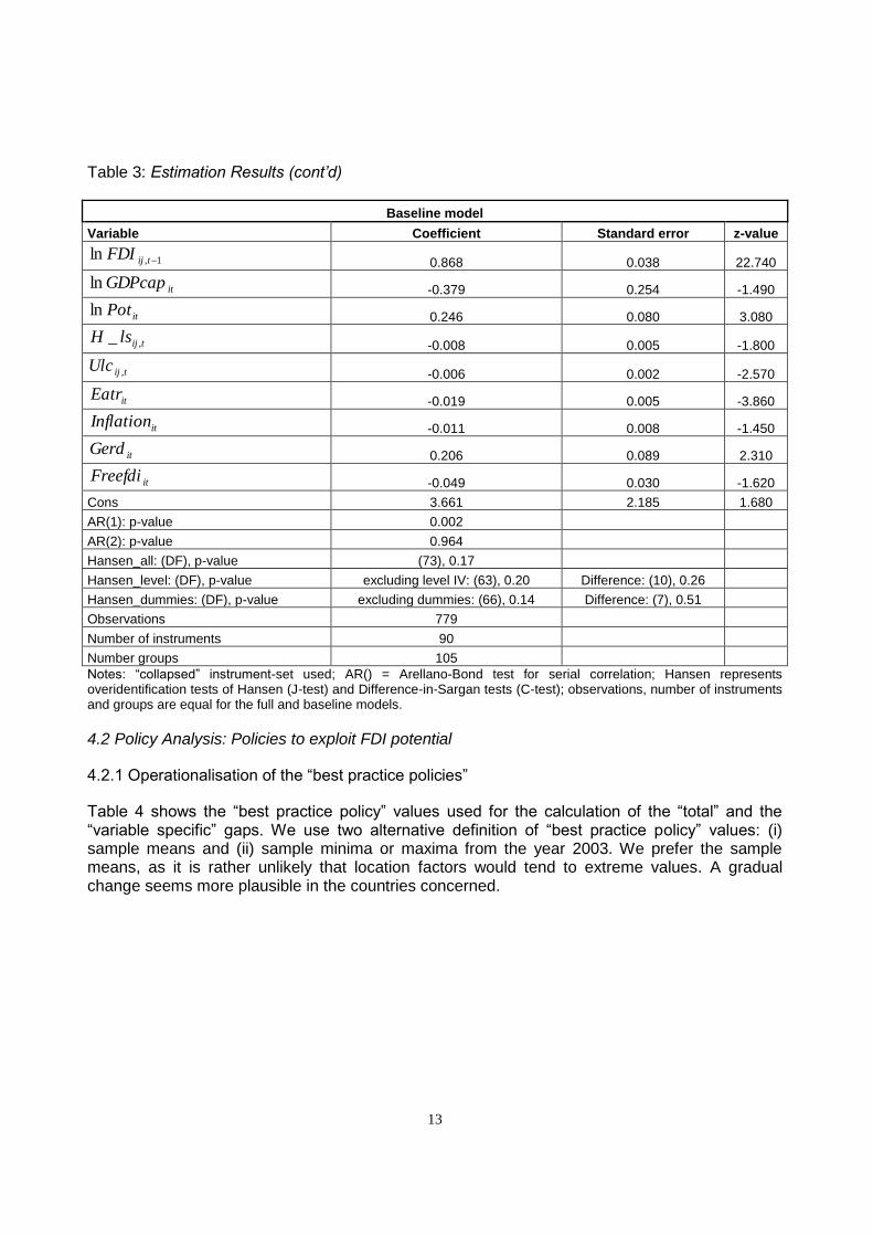
Table 3: Estimation Results (cont’d)

Baseline model

Variable Coefficient Standard error z-value

1,ln tijFDI 0.868 0.038 22.740

itGDPcapln -0.379 0.254 -1.490

itPotln 0.246 0.080 3.080

tijlsH ,_ -0.008 0.005 -1.800

tijUlc , -0.006 0.002 -2.570

itEatr -0.019 0.005 -3.860

itInflation -0.011 0.008 -1.450

itGerd 0.206 0.089 2.310

itFreefdi -0.049 0.030 -1.620

Cons 3.661 2.185 1.680

AR(1): p-value 0.002

AR(2): p-value 0.964

Hansen_all: (DF), p-value (73), 0.17

Hansen_level: (DF), p-value excluding level IV: (63), 0.20 Difference: (10), 0.26

Hansen_dummies: (DF), p-value excluding dummies: (66), 0.14 Difference: (7), 0.51

Observations 779

Number of instruments 90

Number groups 105

Notes: “collapsed” instrument-set used; AR() = Arellano-Bond test for serial correlation; Hansen represents overidentification tests of Hansen (J-test) and Difference-in-Sargan tests (C-test); observations, number of instruments and groups are equal for the full and baseline models.

4.2 Policy Analysis: Policies to exploit FDI potential

4.2.1 Operationalisation of the “best practice policies”

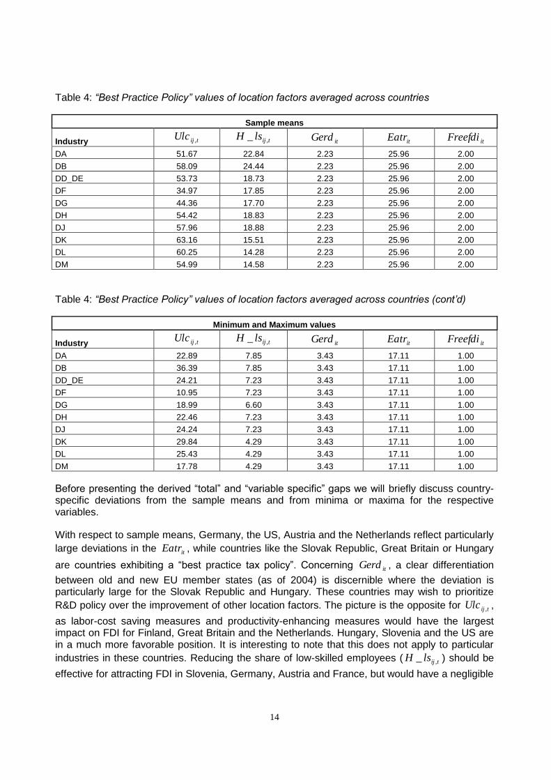
Table 4 shows the “best practice policy” values used for the calculation of the “total” and the “variable specific” gaps. We use two alternative definition of “best practice policy” values: (i) sample means and (ii) sample minima or maxima from the year 2003. We prefer the sample means, as it is rather unlikely that location factors would tend to extreme values. A gradual change seems more plausible in the countries concerned.

14

Table 4: “Best Practice Policy” values of location factors averaged across countries

Sample means

Industry tijUlc , tijlsH ,_ itGerd itEatr itFreefdi

DA 51.67 22.84 2.23 25.96 2.00

DB 58.09 24.44 2.23 25.96 2.00

DD_DE 53.73 18.73 2.23 25.96 2.00

DF 34.97 17.85 2.23 25.96 2.00

DG 44.36 17.70 2.23 25.96 2.00

DH 54.42 18.83 2.23 25.96 2.00

DJ 57.96 18.88 2.23 25.96 2.00

DK 63.16 15.51 2.23 25.96 2.00

DL 60.25 14.28 2.23 25.96 2.00

DM 54.99 14.58 2.23 25.96 2.00

Table 4: “Best Practice Policy” values of location factors averaged across countries (cont’d)

Minimum and Maximum values

Industry tijUlc , tijlsH ,_ itGerd itEatr itFreefdi

DA 22.89 7.85 3.43 17.11 1.00

DB 36.39 7.85 3.43 17.11 1.00

DD_DE 24.21 7.23 3.43 17.11 1.00

DF 10.95 7.23 3.43 17.11 1.00

DG 18.99 6.60 3.43 17.11 1.00

DH 22.46 7.23 3.43 17.11 1.00

DJ 24.24 7.23 3.43 17.11 1.00

DK 29.84 4.29 3.43 17.11 1.00

DL 25.43 4.29 3.43 17.11 1.00

DM 17.78 4.29 3.43 17.11 1.00

Before presenting the derived “total” and “variable specific” gaps we will briefly discuss country-specific deviations from the sample means and from minima or maxima for the respective variables.

With respect to sample means, Germany, the US, Austria and the Netherlands reflect particularly

large deviations in the itEatr , while countries like the Slovak Republic, Great Britain or Hungary

are countries exhibiting a “best practice tax policy”. Concerning itGerd , a clear differentiation

between old and new EU member states (as of 2004) is discernible where the deviation is particularly large for the Slovak Republic and Hungary. These countries may wish to prioritize

R&D policy over the improvement of other location factors. The picture is the opposite for tijUlc , ,

as labor-cost saving measures and productivity-enhancing measures would have the largest impact on FDI for Finland, Great Britain and the Netherlands. Hungary, Slovenia and the US are in a much more favorable position. It is interesting to note that this does not apply to particular

industries in these countries. Reducing the share of low-skilled employees ( tijlsH ,_ ) should be

effective for attracting FDI in Slovenia, Germany, Austria and France, but would have a negligible

15

impact for the other countries in the sample. It would only be possible to increase FDI through the

abolishment or reduction of FDI-specific regulations ( itFreefdi ) in Slovenia and France.

When referring to the minimum and maximum values, Hungary is the for itEatr . Germany, the

US, the Netherlands and Austria are at the upper end, whereas Slovenia and Great Britain are at

the lower end. With respect to itGerd , Finland sets the “best practice policy” value. Not

unexpectedly, the CEEC-4 (Hungary, the Slovak Republic, the Czech Republic, and Slovenia) show the largest deviations, followed by a group of older EU countries: Austria, the Netherlands and Great Britain. On the lower end, i.e. showing small deviations, again not surprisingly we find

the US, Germany and France. For unit labour costs ( tijUlc , ) the Slovak Republic becomes the

benchmark country. On the top end there is no clear clustering of countries, but rather varied

industry-country pairs. Yet the CEEC-4 are clearly clustered at the lower end. With tijlsH ,_ the

Slovak Republic is the benchmark country. Most Slovene industries can be found at the top end (i.e. large deviation), but these are mixed with single industries of the old EU countries and the US. Seven out of the 13 industries with the largest deviations refer to Textiles and Wearing Apparel (DB). The industries of the Netherlands are clustered at the lower end. With respect to

itFreefdi , the Netherlands and Germany are the benchmark countries. Removing obstacles to

cross-border FDI in the form of regulations would primarily increase FDI in Slovenia and France.

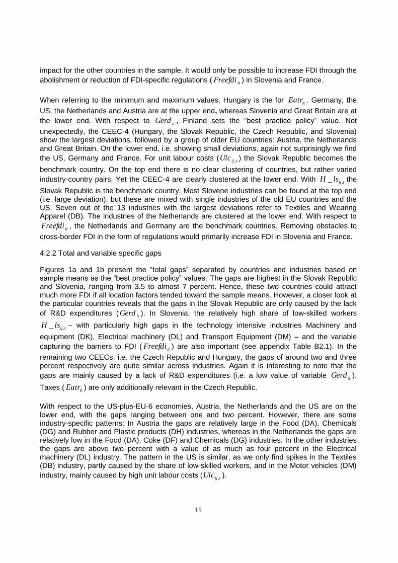
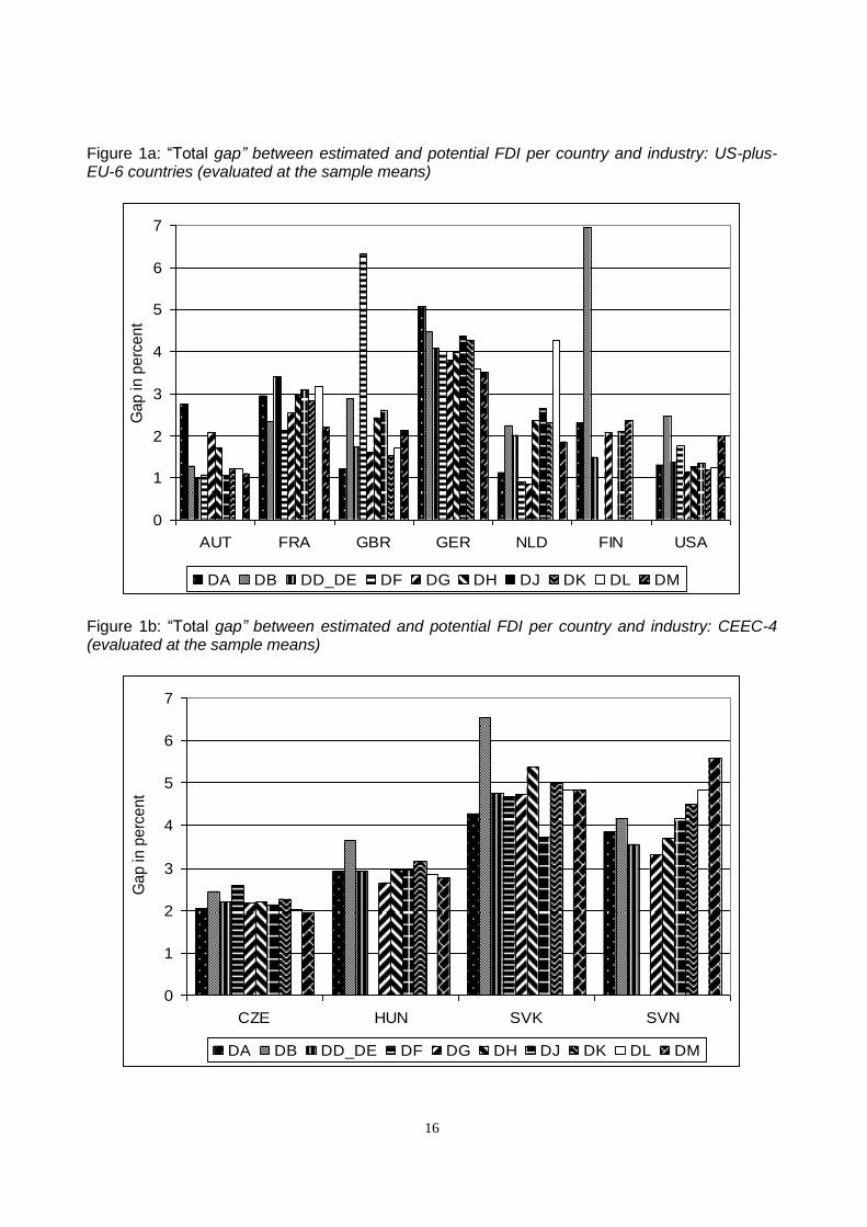
4.2.2 Total and variable specific gaps

Figures 1a and 1b present the “total gaps” separated by countries and industries based on sample means as the “best practice policy” values. The gaps are highest in the Slovak Republic and Slovenia, ranging from 3.5 to almost 7 percent. Hence, these two countries could attract much more FDI if all location factors tended toward the sample means. However, a closer look at the particular countries reveals that the gaps in the Slovak Republic are only caused by the lack

of R&D expenditures ( itGerd ). In Slovenia, the relatively high share of low-skilled workers

tijlsH ,_ – with particularly high gaps in the technology intensive industries Machinery and

equipment (DK), Electrical machinery (DL) and Transport Equipment (DM) – and the variable

capturing the barriers to FDI ( itFreefdi ) are also important (see appendix Table B2.1). In the

remaining two CEECs, i.e. the Czech Republic and Hungary, the gaps of around two and three percent respectively are quite similar across industries. Again it is interesting to note that the

gaps are mainly caused by a lack of R&D expenditures (i.e. a low value of variable itGerd ).

Taxes ( itEatr ) are only additionally relevant in the Czech Republic.

With respect to the US-plus-EU-6 economies, Austria, the Netherlands and the US are on the lower end, with the gaps ranging between one and two percent. However, there are some industry-specific patterns: In Austria the gaps are relatively large in the Food (DA), Chemicals (DG) and Rubber and Plastic products (DH) industries, whereas in the Netherlands the gaps are relatively low in the Food (DA), Coke (DF) and Chemicals (DG) industries. In the other industries the gaps are above two percent with a value of as much as four percent in the Electrical machinery (DL) industry. The pattern in the US is similar, as we only find spikes in the Textiles (DB) industry, partly caused by the share of low-skilled workers, and in the Motor vehicles (DM)

industry, mainly caused by high unit labour costs ( tijUlc , ).

16

Figure 1a: “Total gap” between estimated and potential FDI per country and industry: US-plus-EU-6 countries (evaluated at the sample means)

0

1

2

3

4

5

6

7

AUT FRA GBR GER NLD FIN USA

Ga

p in

pe

rce

nt

DA DB DD_DE DF DG DH DJ DK DL DM

Figure 1b: “Total gap” between estimated and potential FDI per country and industry: CEEC-4 (evaluated at the sample means)

0

1

2

3

4

5

6

7

CZE HUN SVK SVN

Ga

p in

pe

rce

nt

DA DB DD_DE DF DG DH DJ DK DL DM

17

The gaps in the remaining countries are higher, with Germany exhibiting the largest gaps of between four and five percent. The gaps in France range in between two and three percent with low variation across industries. For Great Britain and Finland we find gaps of about two percent with some large differences, especially for the Coke (DF) industry in Great Britain and the Textiles and wearing apparel (DB) industry in Finland.

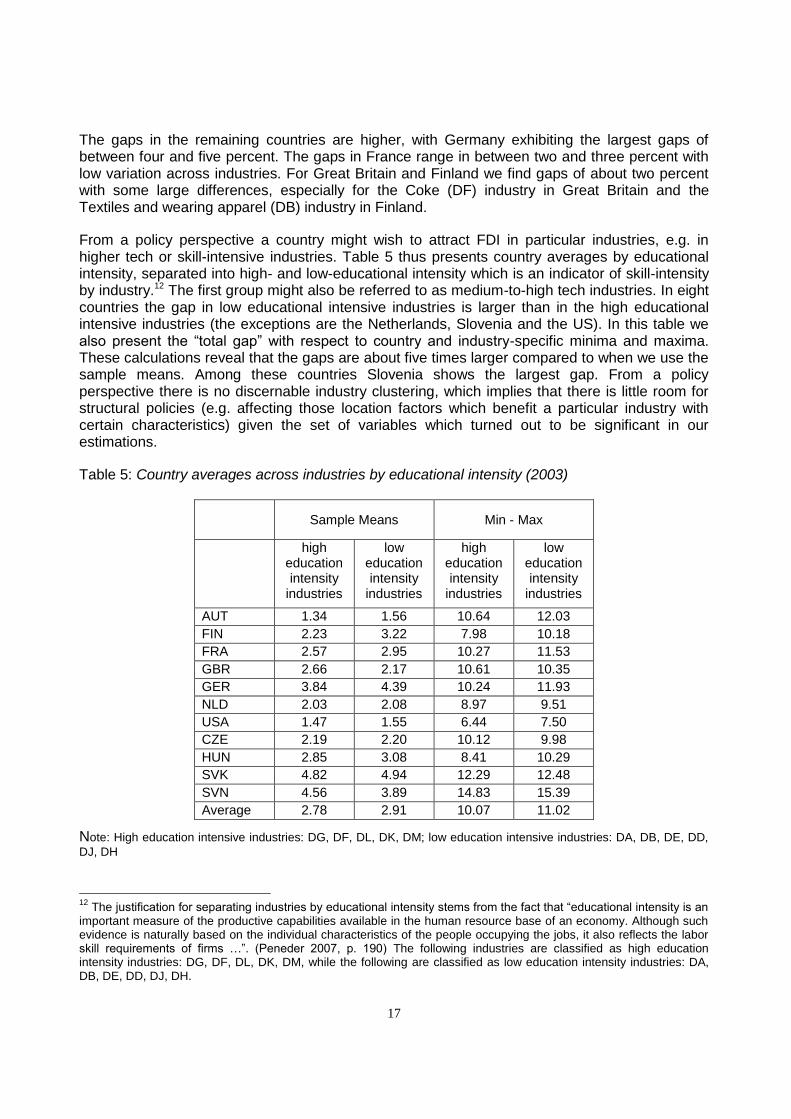
From a policy perspective a country might wish to attract FDI in particular industries, e.g. in higher tech or skill-intensive industries. Table 5 thus presents country averages by educational intensity, separated into high- and low-educational intensity which is an indicator of skill-intensity by industry.12 The first group might also be referred to as medium-to-high tech industries. In eight countries the gap in low educational intensive industries is larger than in the high educational intensive industries (the exceptions are the Netherlands, Slovenia and the US). In this table we also present the “total gap” with respect to country and industry-specific minima and maxima. These calculations reveal that the gaps are about five times larger compared to when we use the sample means. Among these countries Slovenia shows the largest gap. From a policy perspective there is no discernable industry clustering, which implies that there is little room for structural policies (e.g. affecting those location factors which benefit a particular industry with certain characteristics) given the set of variables which turned out to be significant in our estimations.

Table 5: Country averages across industries by educational intensity (2003)

Sample Means Min - Max

high education intensity

industries

low education intensity

industries

high education intensity

industries

low education intensity

industries

AUT 1.34 1.56 10.64 12.03

FIN 2.23 3.22 7.98 10.18

FRA 2.57 2.95 10.27 11.53

GBR 2.66 2.17 10.61 10.35

GER 3.84 4.39 10.24 11.93

NLD 2.03 2.08 8.97 9.51

USA 1.47 1.55 6.44 7.50

CZE 2.19 2.20 10.12 9.98

HUN 2.85 3.08 8.41 10.29

SVK 4.82 4.94 12.29 12.48

SVN 4.56 3.89 14.83 15.39

Average 2.78 2.91 10.07 11.02

Note: High education intensive industries: DG, DF, DL, DK, DM; low education intensive industries: DA, DB, DE, DD,

DJ, DH

12

The justification for separating industries by educational intensity stems from the fact that “educational intensity is an important measure of the productive capabilities available in the human resource base of an economy. Although such evidence is naturally based on the individual characteristics of the people occupying the jobs, it also reflects the labor skill requirements of firms …”. (Peneder 2007, p. 190) The following industries are classified as high education intensity industries: DG, DF, DL, DK, DM, while the following are classified as low education intensity industries: DA, DB, DE, DD, DJ, DH.

18

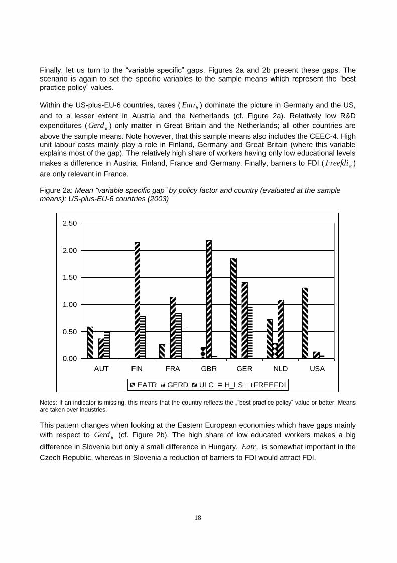
Finally, let us turn to the “variable specific” gaps. Figures 2a and 2b present these gaps. The scenario is again to set the specific variables to the sample means which represent the “best practice policy” values.

Within the US-plus-EU-6 countries, taxes ( itEatr ) dominate the picture in Germany and the US,

and to a lesser extent in Austria and the Netherlands (cf. Figure 2a). Relatively low R&D

expenditures ( itGerd ) only matter in Great Britain and the Netherlands; all other countries are

above the sample means. Note however, that this sample means also includes the CEEC-4. High unit labour costs mainly play a role in Finland, Germany and Great Britain (where this variable explains most of the gap). The relatively high share of workers having only low educational levels

makes a difference in Austria, Finland, France and Germany. Finally, barriers to FDI ( itFreefdi )

are only relevant in France.

Figure 2a: Mean “variable specific gap” by policy factor and country (evaluated at the sample means): US-plus-EU-6 countries (2003)

0.00

0.50

1.00

1.50

2.00

2.50

AUT FIN FRA GBR GER NLD USA

EATR GERD ULC H_LS FREEFDI

Notes: If an indicator is missing, this means that the country reflects the „”best practice policy“ value or better. Means are taken over industries.

This pattern changes when looking at the Eastern European economies which have gaps mainly

with respect to itGerd (cf. Figure 2b). The high share of low educated workers makes a big

difference in Slovenia but only a small difference in Hungary. itEatr is somewhat important in the

Czech Republic, whereas in Slovenia a reduction of barriers to FDI would attract FDI.

19

Figure 2b: Mean “variable specific gap” by policy factor and country (evaluated at the sample means): CEEC-4 (2003)

0.00

1.00

2.00

3.00

4.00

5.00

6.00

CZE HUN SVK SVN

EATR GERD ULC H_LS FREEFDI

Notes: If an indicator is missing, this means that the country reflects the „”best practice policy“ value or better. Means are taken over industries.

5. Summary and Policy Conclusions

The purpose of this paper was, first, to provide information on promising fields of policy intervention when the goal is to attract additional FDI and, second, to provide insight on the scope of FDI that can be attracted if a “best practice policy” is implemented. The results show how different policy variables contribute to closing the gap between actual and potential FDI.

Let us finally discuss the policy conclusion we can draw from the econometric analysis and the evaluation of existing gaps. It is important to bear in mind that the interpretation of our estimates is subject to the ceteris paribus condition.

While the econometric analysis suggests that increasing the itGerd in US-plus-EU-6 economies

would attract more FDI, the analysis of the gaps reveals that these countries may gain more from improvements of other policy variables. Therefore, policies in the US-plus-EU-6 should focus on lowering taxes and improving their unit labour cost position. Changes in unit labour costs might be achieved via productivity effects, e.g. resulting from lowering the share of unskilled workers, as larger wage reduction might not be a viable policy option. Thus, policies in these countries should focus on research and development and the education and training of workers.

For the CEEC-4 not much can be gained (in relative terms) from a further lowering of taxes as

the largest gaps arise from deficiencies in the itGerd (and thus research and development in

general). Instead, policies should strive to increase the share of higher educated workers as this is relatively low compared to that of the US-plus-EU-6 economies.

20

Our analysis has revealed that the two groups of countries in our sample need to focus on different location factors if the gaps are to be closed. Within each group, there is of course some country heterogeneity, as shown in Figures 2a and 2b, which requires a country-specific differentiation of FDI policies. However, as in any other field of economic policy, FDI policy measures are subject to a number of restrictions. In particular, the budgetary effects of policy changes should be considered. As it is unlikely that all location factors in a country will improve simultaneously, this paper provides important information on the role of individual location factors and their impact on FDI.

6. References

Arrelano, M. (2003). Panel Data Econometrics. New York: Oxford University Press.

Barba Navaretti, G. and A.J. Venables (2004, eds). Multinational firms in the world economy. Princeton, N.J.: Princeton University Press.

Barry, F., H. Görg and E. Strobl (2004) Foreign direct investment, agglomerations, and demonstration effects: An empirical investigation, Review of World Economics, 140 (3): 583-600.

Bénassy-Quéré, A., N. Gobalraja and A. Trannoy (2007a). Tax and public input competition. Economic Policy 22 (5): 385–430.

Bénassy-Quéré, A., Coupet, M., Mayer, T. (2007b). Institutional Determinants of Foreign Direct Investment. The World Economy 30 (5): 764–782.

Blonigen, B.A., R.B. Davies and K. Head (2003). Estimating the Knowledge-Capital Model of the Multinational Enterprise: Comment. American Economic Review 93 (3): 980-994.

Blonigen, B.A. (2005). A Review of the Empirical Literature on FDI Determinants. NBER Working Paper Series, Nr. 11299. NBER, Cambridge (Mass.).

Blonigen, B.A., R. B. Davies, G.R. Waddell and H.T. Naughton (2007). FDI in space: Spatial autoregressive relationships in foreign direct investment. European Economic Review 51 (5): 1303-1325.

Blundell, R. and S. Bond (1998). Initial conditions and moment restrictions in dynamic panel data models. Journal of Econometrics 87 (1): 115-143.

Bond, S. (2002). Dynamic panel data models: A guide to micro data methods and practice. Working Paper 09/02. IFS, London.

Clausing, K.A. and C.L. Dorobantu (2005). Re-entering Europe: Does European Union candidacy boost foreign direct investment? Economics of Transition 13 (1): 77–103.

Demekas, D.G., H. Balász, E. Ribakova and Y. Wu (2007). Foreign direct investment in European transition economies – The role of policies. Journal of Comparative Economics 35 (2): 369–386.

DeMooij, R. A. and S. Ederveen (2005). How does foreign direct investment respond to taxes? A meta analysis. Paper presented at the Workshop on FDI and Taxation. GEP Nottingham, October.

21

Devereux, M.P. and R. Griffith (1998). Taxes and the location of production: evidence from a panel of US multinationals. Journal of Public Economics 68 (3): 335-367.

Egger, P. and M. Pfaffermayr (2004). Foreign Direct Investment and European Integration in the 1990s. The World Economy 27 (1): 99–110.

European Commission (2004). Report from the Commission to the Spring European Council COM (2004) 29 final/2.

Markusen, J.R. and K.E. Maskus (2002). Discriminating Among Alternative Theories of the Multinational Enterprise. Review of International Economics 10 (4): 694-707.

Mutti, J.H. (2004). Foreign Direct Investment and Tax Competition. Washington: Institute for International Economics.

Mutti, J. and H. Grubert (2004). Empirical Asymmetries in Foreign Direct Investment and Taxation. Journal of International Economics 62 (2): 337-358.

Pavitt, K. (1984). Sectoral patterns of technical change: Towards a taxonomy and a theory. Research Policy 13 (6): 343-373.

Peneder, M. (2007). A sectoral taxonomy of educational intensity. Empirica 34 (3): 189-212.

Resmini, L. (2000). The determinants of foreign direct investment in the CEECs. Economics of Transition 8 (3): 665-689.

Roodman, D. (2007a). How to do XTABOND? Working Paper, Nr. 103. January. Center for Global Development.

Roodman, D. (2007b). A short note on the Theme of Too Many Instruments. Working Paper, Nr. 125. August. Center for Global Development.

Stöwhase, S. (2005). Tax Rate Differentials and Sector Specific Foreign Direct Investment: Empirical Evidence from the EU. Finanzarchiv 61 (4): 535-558.

Swenson, D. L. (2004). Foreign Investment and the Mediation of Trade Flows. Review of International Economics 12 (4): 609-629.

Timmer, M.P., M.O‟Mahoney and B.v. Ark (2007). EU KLEMS Growth and Productivity Accounts: An Overview. Gronigen Growth and Development Centre, 11/14/2007.

Walkenhorst, P. (2004). Economic Transition and the Sectoral Patterns of Foreign Direct Investment. Emerging Markets Finance and Trade 40 (2): 5-26.

Wheeler, D. and A. Mody (1992). International Investment Location Decisions. Journal of International Economics 33 (1-2): 57-76.

Yeaple, S.R. (2003). The Role of Skill Endowments in the Structure of U.S. outward Foreign Direct Investment. The Review of Economics and Statistics 85 (3): 726-734.

22

Appendix A. Data availability, classifications and correspondences

This appendix covers only those countries for which usable FDI data are available at an industry level. Initially we also checked other countries, but found the data for these to be insufficient, either because there were no data for FDI stocks or because key explanatory variables were missing. The resulting country list is as follows: Austria (AUT), the Czech Republic (CZE), France (FRA), Finland (FIN), Great Britain (GBR), Germany (GER), Hungary (HUN), the Netherlands (NLD), Slovenia (SVN), the Slovak Republic (SVK) and the United States of America (USA).

A.1. Dependent variable: Industry-level FDI stocks

Data for FDI inward stocks are mainly taken from the OECD IDI database. This database provides data either in US-$ or in 'submitted currency' (the latter corresponds in all cases to the respective national currency, with the exception of Poland). The classification of industries is according to ISIC revision 3, which also corresponds to NACE revision 1 (15-37). These are listed in table A.1.1 below. In this table we also show the correspondence to the recently released EU KLEMS database from which some of the explanatory variables are taken. The industry classification in the EU KLEMS database is derived from the NACE revision 1 classification. The descriptions of industries according to the NACE or ISIC classification respectively, are presented in Table A.1.2. FDI data for the CEEC-4 are taken from the wiiw FDI database (see www.wiiw.org) which reports industry-level data at the NACE level. Note that for both 15-37 and DA-

DN classification the scope differs across countries.

Table A1.1 Industry correspondences

Number Description (in OECD IDI) ISIC rev. 3 NACE rev. 1 EUKLEMS

01 Food products 15,16 DA 15t16

02 Textiles and wearing apparel 17,18 DB 17t18

03 Wood, publishing and printing 20, 21, 22 DD, DE 20,21t22

04 Total (02+03)

05 Refined petroleum and other treatments 23 DF 23

06 Chemical products 24 DG 24

07 Pharmaceuticals, medicinal chemical and botanical products

08 Rubber and plastic products 25 DH 25

09 Total (05+06+08)

10 Metal products 27, 28 DJ 27t28

11 Mechanical products 29 DK 29

12 Total (10+11)

13 Office machinery and computers 30 DL 30t33

14 Radio, TV, communication equipment 32

15 Total (13+14)

16 Medical precision and optical

instruments, watches and clocks 33

17 Motor vehicles 34

18 Other transport equipment 35

19 Manufacture of aircraft and spacecraft

20 Total (17+18) DM 34t35

21 Other manufacturing 36, 37

23

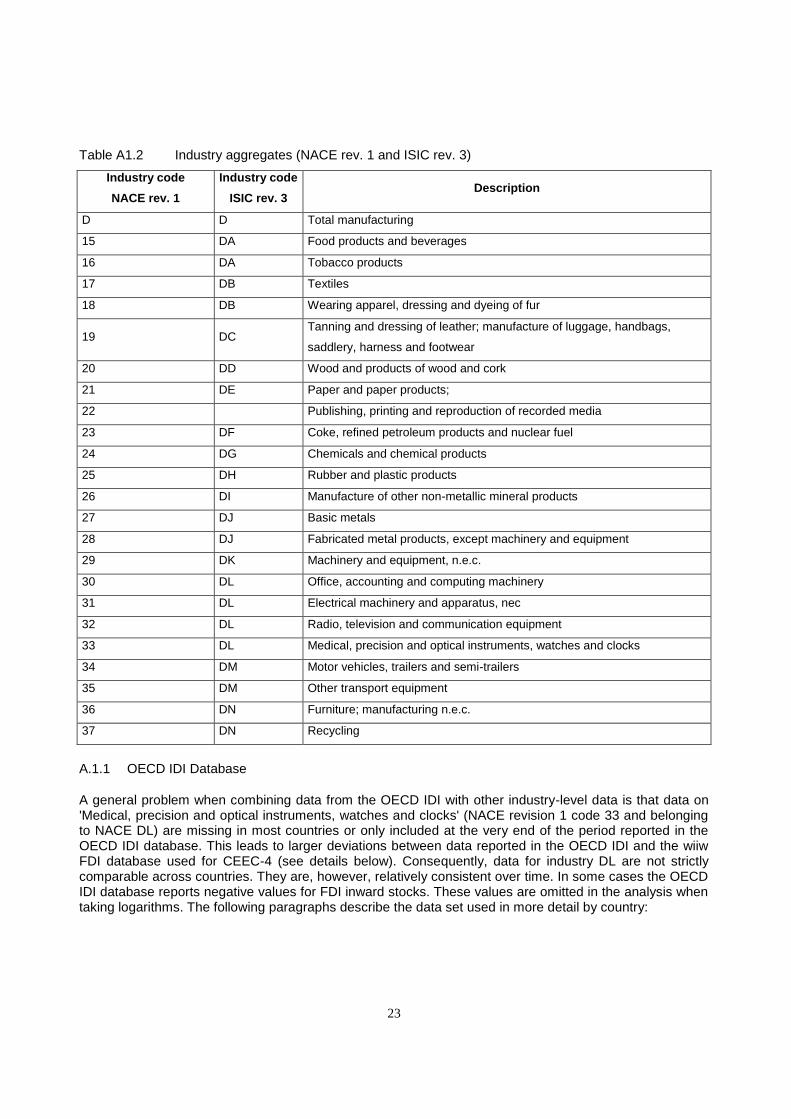
Table A1.2 Industry aggregates (NACE rev. 1 and ISIC rev. 3)

Industry code

NACE rev. 1

Industry code

ISIC rev. 3 Description

D D Total manufacturing

15 DA Food products and beverages

16 DA Tobacco products

17 DB Textiles

18 DB Wearing apparel, dressing and dyeing of fur

19 DC Tanning and dressing of leather; manufacture of luggage, handbags,

saddlery, harness and footwear

20 DD Wood and products of wood and cork

21 DE Paper and paper products;

22 Publishing, printing and reproduction of recorded media

23 DF Coke, refined petroleum products and nuclear fuel

24 DG Chemicals and chemical products

25 DH Rubber and plastic products

26 DI Manufacture of other non-metallic mineral products

27 DJ Basic metals

28 DJ Fabricated metal products, except machinery and equipment

29 DK Machinery and equipment, n.e.c.

30 DL Office, accounting and computing machinery

31 DL Electrical machinery and apparatus, nec

32 DL Radio, television and communication equipment

33 DL Medical, precision and optical instruments, watches and clocks

34 DM Motor vehicles, trailers and semi-trailers

35 DM Other transport equipment

36 DN Furniture; manufacturing n.e.c.

37 DN Recycling

A.1.1 OECD IDI Database

A general problem when combining data from the OECD IDI with other industry-level data is that data on 'Medical, precision and optical instruments, watches and clocks' (NACE revision 1 code 33 and belonging to NACE DL) are missing in most countries or only included at the very end of the period reported in the OECD IDI database. This leads to larger deviations between data reported in the OECD IDI and the wiiw FDI database used for CEEC-4 (see details below). Consequently, data for industry DL are not strictly comparable across countries. They are, however, relatively consistent over time. In some cases the OECD IDI database reports negative values for FDI inward stocks. These values are omitted in the analysis when taking logarithms. The following paragraphs describe the data set used in more detail by country:

24

Austria

'Refined petroleum and other treatments' was missing in 2003 and was replaced by extrapolation. The FDI

inward stock almost doubled in 2002; 'Office machinery and equipment' was missing in 1996 and was

replaced by linear extrapolation; entries in 'Radio, TV and communication equipment' are negative in 1997

and 1998; entries in 'Other transport equipment' are negative in the period 1997 to 2000.

Finland

Data for 'Textiles and wearing apparel' and 'Wood, publishing and printing' are linearly interpolated for 2000-2002. Data are either not available or only available for 2003 and 2004 for 'Refined petroleum and other treatments', 'Rubber and plastic products', 'Office machinery and computers', and 'Radio, TV, and communication equipment', 'Medical, precision and optical instruments, watches and clocks', 'Motor vehicles', 'Other transport equipments'; data for some subaggregates available; negative values appear in 1998.

Great Britain

Data for 'Refined petroleum and other treatments' are interpolated in 1997 and 1998 and extrapolated for 2003; 'Rubber and plastic products' is calculated as difference to the subtotal provided.

France, Germany, Netherlands

No adjustments were made.

USA

The subtotal for 'Textiles and wearing apparel' and 'Wood, publishing and printing' is recalculated as it originally also includes 'Food products'; the subtotals for chemical sector and metal and machinery sector are calculated from detailed industry data; industry 'Medical, precision and optical instruments, watches and clocks' is only available from 2002.

A.1.2 WIIW Database

For CEEC-4 (CZE, HUN, SVK, SVN) we relied on the 'wiiw Database on Foreign Direct Investment 2007', the reason being the higher reliability and the longer period covered for most countries. This database provides FDI inward stocks in the manufacturing at the NACE 2-digit level in either codes 15-37 or letter codes DA-DN up to 2006. We only consider the period up to 2003 to be consistent with the OECD IDI data. The following reports differences of wiiw data and the OECD IDI database described above:

Czech Republic

Period covered is 1997-2003; data in OECD IDI and wiiw FDI database are almost identical (some smaller deviations in some years), the only exception being industry DL as in the latter database 'Medical precision and optical instruments, watches and clocks' (33) are missing; however, differences become smaller over time.

25

Hungary

The period covered is 1998-2003; the data in the OECD IDI and wiiw FDI are almost identical from 2001 onwards; before 2001, the data in the OECD IDI are missing in 1999 and 2000 and seem to be unreliable from 1995-1998 in the OECD IDI database (a large jump is reported between 1998 and 1999); larger

deviations are found in industry DL as in the latter database 'Medical precision and optical instruments,

watches and clocks' (33) are missing, however differences become smaller over time.

Slovak Republic

The period covered is 1996-2003.

Slovenia

The period covered is 1995-2003; data are missing for industry DF due to confidentiality.

Using this information one is left with data on FDI inward stocks for eleven countries and ten industries. The time period covered is 1995-2003 (although for some countries not all years are available); with respect to industry detail we distinguish ten industries within the manufacturing sector: Food products (DA), Textiles and Wearing Apparel (DB), Wood and paper products (DD_DE), Coke and Petroleum (DF), Chemicals and chemical products (DG), Rubber and plastic products (DH), Basic and fabricated metal products (DJ), Machinery and equipment (DK), Electrical machinery (DL), and Motor vehicles and transport equipment (DM).

13

A2. Explanatory variables

A2.1. Industry-level data

Data at the industry level are calculated using the EU KLEMS database (see www.euklems.org and Timmer et al. 2007). Unit labour costs have been calculated as ((COMP/EXRavg) / (H_EMPE) / ((VA / PPP_15) / H_EMP) where COMP denotes “compensation of employees” (in millions of local currency), VA is “gross value added” at current basic prices (in millions of local currency); H_EMP and H_EMPE denote “total hours worked” by persons engaged (millions) and “total hours worked” by employees (millions) respectively. In addition to this, the share of low educated workers was calculated, provided the information was available in this database.

13

Note that Poland has not been included in the sample as it receives comparably few FDI in per capita terms in the manufacturing sector. Thus, it would be an outlier in our sample.

26

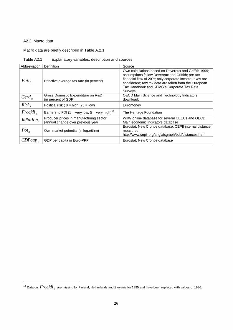
A2.2. Macro data

Macro data are briefly described in Table A.2.1.

Table A2.1 Explanatory variables: description and sources

Abbreviation Definition Source

itEatr Effective average tax rate (in percent)

Own calculations based on Devereux and Griffith 1999; assumptions follow Devereux and Griffith; pre-tax financial flow of 20%; only corporate income taxes are considered; raw tax data are taken from the European Tax Handbook and KPMG‟s Corporate Tax Rate Surveys;

itGerd Gross Domestic Expenditure on R&D (in percent of GDP)

OECD Main Science and Technology Indicators download;

itRisk Political risk ( 0 = high; 25 = low) Euromoney

itFreefdi Barriers to FDI (1 = very low; 5 = very high)14

The Heritage Foundation

itInflation Producer prices in manufacturing sector (annual change over previous year)

WIIW online database for several CEECs and OECD Main economic indicators database

itPot Own market potential (in logarithm) Eurostat: New Cronos database; CEPII internal distance measures: http://www.cepii.org/anglaisgraph/bdd/distances.html

itGDPcap GDP per capita in Euro-PPP Eurostat: New Cronos database

14

Data on itFreefdi are missing for Finland, Netherlands and Slovenia for 1995 and have been replaced with values of 1996.

27

Appendix B. Figures and Tables

B1. Descriptive Statistics

Table B1.1 Means, Standard Deviation, Minima and Maxima

Variable Mean Std. Dev. Min Max

tijFDI ,ln Overall 7.20 1.98 0.74 11.89

Between 1.91 3.07 11.50

Within 0.48 4.31 9.46

1,ln tijFDI Overall 7.06 2.02 0.64 11.89

Between 1.96 1.94 11.42

Within 0.50 4.39 10.43

itGDPcapln Overall 9.89 0.34 9.10 10.41

Between 0.34 9.24 10.31

Within 0.10 9.66 10.06

itPotln Overall 7.63 1.31 5.43 9.18

Between 1.32 5.60 9.11

Within 0.14 7.25 7.89

tijlsH ,_ Overall 20.18 8.83 4.29 40.50

Between 8.62 6.21 34.84

Within 1.59 14.37 26.68

tijUlc ,

Overall 57.24 23.38 -29.71 113.42

Between 23.46 4.85 99.80

Within 5.75 22.67 91.67

itEatr Overall 27.70 5.74 17.11 38.27

Between 5.49 17.36 36.08

Within 2.23 19.77 34.94

itInflation Overall 1.99 3.18 -2.68 11.60

Between 2.07 -0.31 5.69

Within 2.44 -4.83 11.43

itGerd Overall 1.85 0.67 0.57 3.43

Between 0.68 0.70 3.08

Within 0.13 1.28 2.21

itFreefdi Overall 2.16 0.56 1.00 4.00

Between 0.44 1.63 3.00

Within 0.32 1.28 3.28

itRisk Overall 21.78 3.86 12.32 25.00

Between 3.90 13.81 24.71

Within 0.70 19.78 24.14

N = 779 n = 105 T-bar = 7.42

28

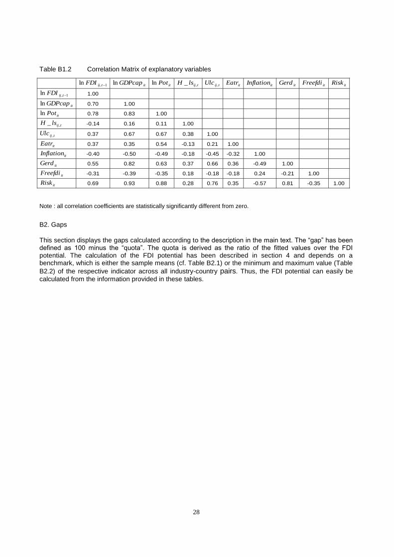
Table B1.2 Correlation Matrix of explanatory variables

Note : all correlation coefficients are statistically significantly different from zero.

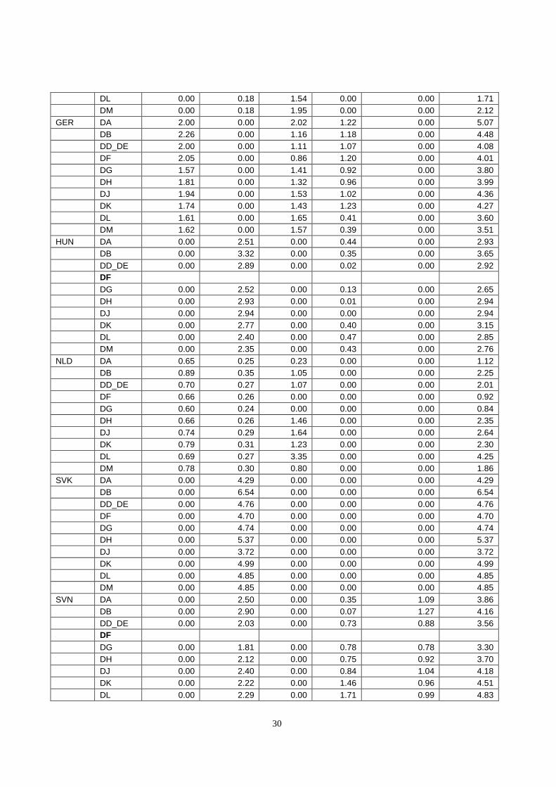
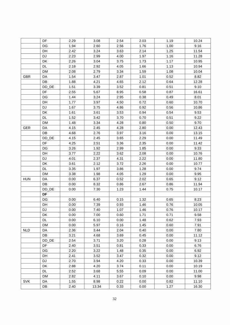
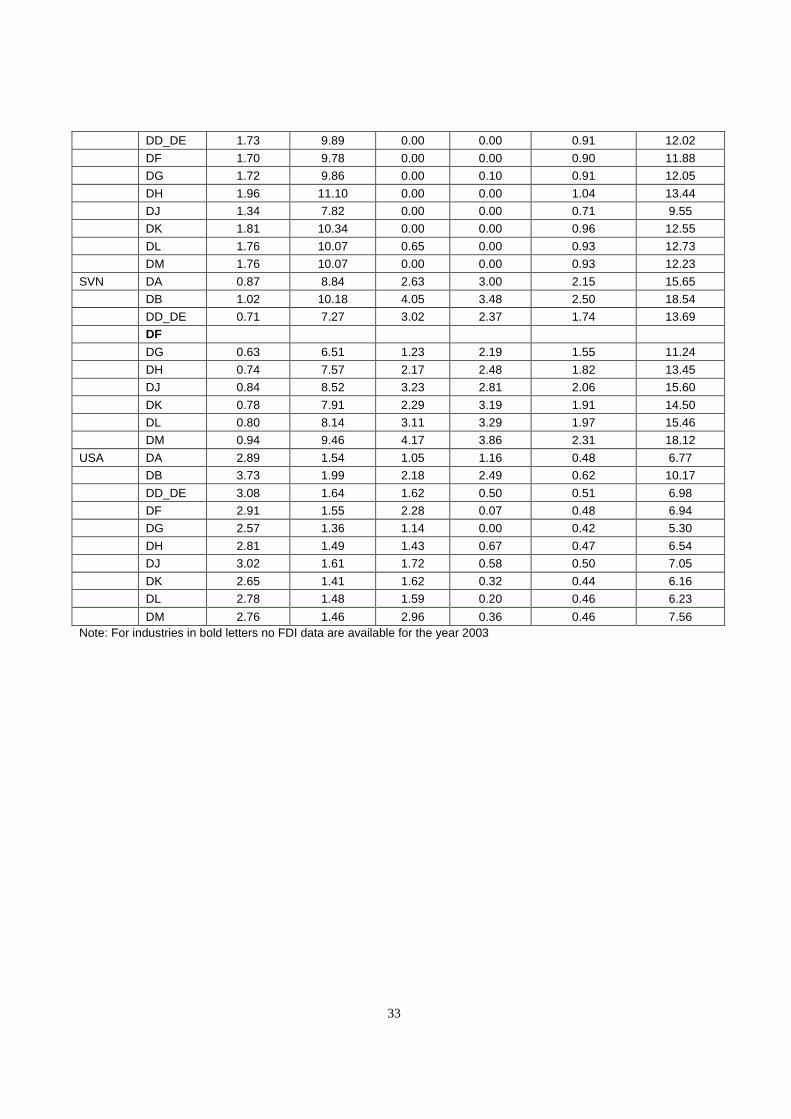
B2. Gaps

This section displays the gaps calculated according to the description in the main text. The “gap” has been defined as 100 minus the “quota”. The quota is derived as the ratio of the fitted values over the FDI potential. The calculation of the FDI potential has been described in section 4 and depends on a benchmark, which is either the sample means (cf. Table B2.1) or the minimum and maximum value (Table

B2.2) of the respective indicator across all industry-country pairs. Thus, the FDI potential can easily be

calculated from the information provided in these tables.

1,ln tijFDI itGDPcapln itPotln tijlsH ,_ tijUlc ,

itEatr itInflation itGerd itFreefdi itRisk

1,ln tijFDI 1.00

itGDPcapln 0.70 1.00

itPotln 0.78 0.83 1.00

tijlsH ,_ -0.14 0.16 0.11 1.00

tijUlc ,

0.37 0.67 0.67 0.38 1.00

itEatr 0.37 0.35 0.54 -0.13 0.21 1.00

itInflation -0.40 -0.50 -0.49 -0.18 -0.45 -0.32 1.00

itGerd 0.55 0.82 0.63 0.37 0.66 0.36 -0.49 1.00

itFreefdi -0.31 -0.39 -0.35 0.18 -0.18 -0.18 0.24 -0.21 1.00

itRisk 0.69 0.93 0.88 0.28 0.76 0.35 -0.57 0.81 -0.35 1.00

29

Table B2.1 Gaps based on Sample Means, 2003, by policy variables

Country Industry EATR GERD ULC H_LS FREEFDI All variables

AUT DA 0.58 0.00 1.53 0.69 0.00 2.76

DB 0.70 0.00 0.00 0.59 0.00 1.28

DD_DE 0.56 0.00 0.00 0.44 0.00 0.99

DF 0.55 0.00 0.00 0.54 0.00 1.08

DG 0.51 0.00 1.08 0.52 0.00 2.08

DH 0.70 0.00 0.50 0.54 0.00 1.72

DJ 0.60 0.00 0.00 0.46 0.00 1.05

DK 0.56 0.00 0.32 0.33 0.00 1.20

DL 0.53 0.00 0.25 0.45 0.00 1.22

DM 0.62 0.00 0.00 0.49 0.00 1.10

CZE DA 0.35 1.71 0.00 0.00 0.00 2.05

DB 0.42 2.06 0.00 0.00 0.00 2.46

DD_DE 0.37 1.83 0.00 0.00 0.00 2.19

DF 0.44 2.16 0.00 0.00 0.00 2.58

DG 0.37 1.81 0.00 0.00 0.00 2.16

DH 0.37 1.84 0.00 0.00 0.00 2.20

DJ 0.36 1.78 0.00 0.00 0.00 2.13

DK 0.38 1.89 0.00 0.00 0.00 2.26

DL 0.34 1.68 0.00 0.00 0.00 2.01

DM 0.33 1.63 0.00 0.00 0.00 1.96

FIN DA 0.00 0.00 1.51 0.82 0.00 2.30

DB 0.00 0.00 5.90 1.20 0.00 6.96

DD_DE 0.00 0.00 0.72 0.79 0.00 1.50

DF

DG 0.00 0.00 1.23 0.87 0.00 2.08

DH

DJ 0.00 0.00 1.36 0.77 0.00 2.11

DK 0.00 0.00 2.18 0.20 0.00 2.37

DL

DM

FRA DA 0.26 0.00 1.37 0.81 0.57 2.94

DB 0.32 0.00 0.53 0.82 0.71 2.34

DD_DE 0.27 0.00 1.68 0.93 0.61 3.40

DF 0.27 0.00 0.30 1.00 0.60 2.13

DG 0.23 0.00 0.99 0.85 0.50 2.53

DH 0.28 0.00 1.18 0.95 0.63 2.98

DJ 0.26 0.00 1.45 0.87 0.58 3.09

DK 0.26 0.00 1.38 0.65 0.59 2.83

DL 0.25 0.00 1.68 0.74 0.57 3.17

DM 0.24 0.00 0.77 0.68 0.54 2.20

GBR DA 0.00 0.18 1.03 0.00 0.00 1.21

DB 0.00 0.22 2.28 0.40 0.00 2.88

DD_DE 0.00 0.18 1.56 0.00 0.00 1.73

DF 0.00 0.31 6.07 0.00 0.00 6.33

DG 0.00 0.17 1.45 0.00 0.00 1.61

DH 0.00 0.21 2.22 0.00 0.00 2.42

DJ 0.00 0.20 2.42 0.00 0.00 2.61

DK 0.00 0.19 1.34 0.00 0.00 1.52

30

DL 0.00 0.18 1.54 0.00 0.00 1.71

DM 0.00 0.18 1.95 0.00 0.00 2.12

GER DA 2.00 0.00 2.02 1.22 0.00 5.07

DB 2.26 0.00 1.16 1.18 0.00 4.48

DD_DE 2.00 0.00 1.11 1.07 0.00 4.08

DF 2.05 0.00 0.86 1.20 0.00 4.01

DG 1.57 0.00 1.41 0.92 0.00 3.80

DH 1.81 0.00 1.32 0.96 0.00 3.99

DJ 1.94 0.00 1.53 1.02 0.00 4.36

DK 1.74 0.00 1.43 1.23 0.00 4.27

DL 1.61 0.00 1.65 0.41 0.00 3.60

DM 1.62 0.00 1.57 0.39 0.00 3.51

HUN DA 0.00 2.51 0.00 0.44 0.00 2.93

DB 0.00 3.32 0.00 0.35 0.00 3.65

DD_DE 0.00 2.89 0.00 0.02 0.00 2.92

DF

DG 0.00 2.52 0.00 0.13 0.00 2.65

DH 0.00 2.93 0.00 0.01 0.00 2.94

DJ 0.00 2.94 0.00 0.00 0.00 2.94

DK 0.00 2.77 0.00 0.40 0.00 3.15

DL 0.00 2.40 0.00 0.47 0.00 2.85

DM 0.00 2.35 0.00 0.43 0.00 2.76

NLD DA 0.65 0.25 0.23 0.00 0.00 1.12

DB 0.89 0.35 1.05 0.00 0.00 2.25

DD_DE 0.70 0.27 1.07 0.00 0.00 2.01

DF 0.66 0.26 0.00 0.00 0.00 0.92

DG 0.60 0.24 0.00 0.00 0.00 0.84

DH 0.66 0.26 1.46 0.00 0.00 2.35

DJ 0.74 0.29 1.64 0.00 0.00 2.64

DK 0.79 0.31 1.23 0.00 0.00 2.30

DL 0.69 0.27 3.35 0.00 0.00 4.25

DM 0.78 0.30 0.80 0.00 0.00 1.86

SVK DA 0.00 4.29 0.00 0.00 0.00 4.29

DB 0.00 6.54 0.00 0.00 0.00 6.54

DD_DE 0.00 4.76 0.00 0.00 0.00 4.76

DF 0.00 4.70 0.00 0.00 0.00 4.70

DG 0.00 4.74 0.00 0.00 0.00 4.74

DH 0.00 5.37 0.00 0.00 0.00 5.37

DJ 0.00 3.72 0.00 0.00 0.00 3.72

DK 0.00 4.99 0.00 0.00 0.00 4.99

DL 0.00 4.85 0.00 0.00 0.00 4.85

DM 0.00 4.85 0.00 0.00 0.00 4.85

SVN DA 0.00 2.50 0.00 0.35 1.09 3.86

DB 0.00 2.90 0.00 0.07 1.27 4.16

DD_DE 0.00 2.03 0.00 0.73 0.88 3.56

DF

DG 0.00 1.81 0.00 0.78 0.78 3.30

DH 0.00 2.12 0.00 0.75 0.92 3.70

DJ 0.00 2.40 0.00 0.84 1.04 4.18

DK 0.00 2.22 0.00 1.46 0.96 4.51

DL 0.00 2.29 0.00 1.71 0.99 4.83

31

DM 0.00 2.68 0.00 1.95 1.17 5.59

USA DA 1.30 0.00 0.00 0.00 0.00 1.30

DB 1.68 0.00 0.00 0.82 0.00 2.47

DD_DE 1.38 0.00 0.00 0.00 0.00 1.38

DF 1.30 0.00 0.47 0.00 0.00 1.76

DG 1.15 0.00 0.00 0.00 0.00 1.15

DH 1.26 0.00 0.00 0.00 0.00 1.26

DJ 1.35 0.00 0.00 0.00 0.00 1.35

DK 1.19 0.00 0.00 0.00 0.00 1.19

DL 1.25 0.00 0.00 0.00 0.00 1.25

DM 1.23 0.00 0.79 0.00 0.00 2.00

Note: For industries in bold letters no FDI data are available for the year 2003

Table B2.2 Gaps based on Sample Minima and Maxima, 2003, by policy variables

Country industry EATR GERD ULC H_LS FREEFDI All variables

AUT DA 3.03 3.55 4.06 2.46 0.73 12.50

DB 3.59 4.21 2.35 2.92 0.87 12.59

DD_DE 2.89 3.39 2.55 1.75 0.69 10.38

DF 2.86 3.35 2.06 1.73 0.69 9.88

DG 2.68 3.14 3.07 1.68 0.64 10.32

DH 3.60 4.22 3.90 2.19 0.87 13.28

DJ 3.11 3.64 3.11 1.88 0.75 11.40

DK 2.90 3.41 3.18 1.62 0.70 10.83

DL 2.73 3.20 3.06 1.52 0.65 10.30

DM 3.20 3.76 3.53 1.79 0.77 11.88

CZE DA 2.58 5.72 0.00 0.50 0.66 9.00

DB 3.10 6.82 0.00 0.61 0.80 10.66

DD_DE 2.76 6.11 1.14 0.49 0.71 10.48

DF 3.25 7.15 1.17 0.58 0.84 12.03

DG 2.73 6.04 0.23 0.56 0.70 9.69

DH 2.78 6.14 0.18 0.49 0.71 9.74

DJ 2.69 5.95 0.89 0.48 0.69 10.03

DK 2.85 6.30 0.80 0.42 0.73 10.42

DL 2.54 5.64 0.72 0.37 0.65 9.37

DM 2.47 5.48 0.67 0.36 0.63 9.10

FIN DA 1.69 0.00 3.70 2.35 0.63 7.92

DB 3.07 0.00 9.80 4.23 1.15 16.39

DD_DE 1.90 0.00 3.48 2.11 0.71 7.75

DF

DG 1.83 0.00 3.33 2.10 0.68 7.52

DH

DJ 1.91 0.00 4.47 2.12 0.71 8.67

DK 1.85 0.00 4.89 1.47 0.69 8.43

DL

DM

FRA DA 2.19 2.94 3.36 2.19 1.13 10.83

DB 2.72 3.65 3.26 2.72 1.41 12.42

DD_DE 2.33 3.12 4.01 2.06 1.21 11.59

32

DF 2.29 3.08 2.54 2.03 1.19 10.24

DG 1.94 2.60 2.56 1.76 1.00 9.16

DH 2.42 3.24 3.63 2.14 1.25 11.54

DJ 2.23 2.99 4.00 1.97 1.16 11.28

DK 2.26 3.04 3.75 1.73 1.17 10.95

DL 2.18 2.92 4.05 1.66 1.13 10.94

DM 2.08 2.79 3.34 1.59 1.08 10.04

GBR DA 1.54 3.47 2.87 1.01 0.52 8.82

DB 1.88 4.21 4.65 2.12 0.64 12.28

DD_DE 1.51 3.39 3.52 0.81 0.51 9.10

DF 2.55 5.67 8.95 0.58 0.87 16.61

DG 1.44 3.24 2.95 0.38 0.49 8.01

DH 1.77 3.97 4.50 0.72 0.60 10.70

DJ 1.67 3.75 4.86 0.92 0.56 10.86

DK 1.61 3.61 3.53 0.94 0.54 9.53

DL 1.52 3.42 3.70 0.70 0.51 9.22

DM 1.48 3.34 4.28 0.80 0.50 9.70

GER DA 4.15 2.45 4.28 2.80 0.00 12.43

DB 4.68 2.76 3.97 3.16 0.00 13.15

DD_DE 4.15 2.45 3.65 2.29 0.00 11.49

DF 4.25 2.51 3.36 2.35 0.00 11.42

DG 3.26 1.92 2.99 1.85 0.00 9.33

DH 3.77 2.22 3.62 2.08 0.00 10.76

DJ 4.01 2.37 4.31 2.22 0.00 11.80

DK 3.61 2.12 3.72 2.26 0.00 10.77

DL 3.35 1.97 3.86 1.28 0.00 9.74

DM 3.38 1.98 4.05 1.29 0.00 9.95

HUN DA 0.00 6.37 0.52 2.02 0.65 9.12

DB 0.00 8.32 0.86 2.67 0.86 11.94

DD_DE 0.00 7.30 1.23 1.44 0.75 10.17

DF

DG 0.00 6.40 0.15 1.32 0.65 8.23

DH 0.00 7.39 0.93 1.46 0.76 10.05

DJ 0.00 7.40 1.07 1.46 0.76 10.17

DK 0.00 7.00 0.60 1.71 0.71 9.58

DL 0.00 6.10 0.00 1.48 0.62 7.93

DM 0.00 5.97 0.16 1.45 0.60 7.91

NLD DA 2.36 3.44 2.04 0.40 0.00 7.80

DB 3.21 4.68 3.69 0.45 0.00 11.12

DD_DE 2.54 3.71 3.20 0.28 0.00 9.13

DF 2.40 3.51 0.81 0.33 0.00 6.76

DG 2.20 3.22 1.48 0.35 0.00 6.92

DH 2.41 3.52 3.47 0.32 0.00 9.12

DJ 2.70 3.94 4.20 0.33 0.00 10.39

DK 2.88 4.20 3.74 0.11 0.00 10.19

DL 2.52 3.68 5.55 0.09 0.00 11.00

DM 2.82 4.11 3.67 0.10 0.00 9.98

SVK DA 1.55 8.98 0.22 0.00 0.82 11.10

DB 2.40 13.34 0.33 0.00 1.27 16.30

33

DD_DE 1.73 9.89 0.00 0.00 0.91 12.02

DF 1.70 9.78 0.00 0.00 0.90 11.88

DG 1.72 9.86 0.00 0.10 0.91 12.05

DH 1.96 11.10 0.00 0.00 1.04 13.44

DJ 1.34 7.82 0.00 0.00 0.71 9.55

DK 1.81 10.34 0.00 0.00 0.96 12.55

DL 1.76 10.07 0.65 0.00 0.93 12.73

DM 1.76 10.07 0.00 0.00 0.93 12.23

SVN DA 0.87 8.84 2.63 3.00 2.15 15.65

DB 1.02 10.18 4.05 3.48 2.50 18.54

DD_DE 0.71 7.27 3.02 2.37 1.74 13.69

DF

DG 0.63 6.51 1.23 2.19 1.55 11.24

DH 0.74 7.57 2.17 2.48 1.82 13.45

DJ 0.84 8.52 3.23 2.81 2.06 15.60

DK 0.78 7.91 2.29 3.19 1.91 14.50

DL 0.80 8.14 3.11 3.29 1.97 15.46

DM 0.94 9.46 4.17 3.86 2.31 18.12

USA DA 2.89 1.54 1.05 1.16 0.48 6.77

DB 3.73 1.99 2.18 2.49 0.62 10.17

DD_DE 3.08 1.64 1.62 0.50 0.51 6.98

DF 2.91 1.55 2.28 0.07 0.48 6.94

DG 2.57 1.36 1.14 0.00 0.42 5.30

DH 2.81 1.49 1.43 0.67 0.47 6.54

DJ 3.02 1.61 1.72 0.58 0.50 7.05

DK 2.65 1.41 1.62 0.32 0.44 6.16

DL 2.78 1.48 1.59 0.20 0.46 6.23

DM 2.76 1.46 2.96 0.36 0.46 7.56

Note: For industries in bold letters no FDI data are available for the year 2003