pooled time series

Federico Podestà

RECENT DEVELOPMENTS IN QUANTITATIVECOMPARATIVE METHODOLOGY: THE CASE OF POOLED TIME SERIES

CROSS-SECTION ANALYSIS

DSS PAPERS SOC 3-02

INDICE

1. Advantages and Disadvantages of Pooled Analysis .......... Pag. 6

2. The Estimation Issue: GLS vs. OLS ........................................ 13

3. Time and Space Effects ............................................................. 21

4. Pooling Dilemma and Casual Heterogeneity ........................... 27

5. Pooled TSCS analysis in STATA software .............................. 35

Bibliography ............................................................................... 41

The first draft of this paper has been written at McDonough School of Business(Georgetown University) in November 2000. For this reason, I would like tothank Professor Dennis Quinn for the opportunity he allowed me.

Recent Developments in Quantitative Comparative Methodology 5

Students of the political economy have tended to investigate relationship

between institutions and economic variables by comparing observations across

space or observations over time. Until recently, the space and the time domains

have rarely been combinated in the comparative research. However, new

quantitative methods stress sensitivity to time as well as space. Pooled time

series cross-section analysis (TSCS) is probably the most important way to

examine simultaneously these dimensions.

In this paper, I will try to describe the “state of the art” of this approach

discussing first the characteristics of TSCS data and advantages and

disadvantages of this statistical technique (Section 1). Hence, I will discuss

main issues that relate to the estimation method (section 2). After that, I will

address the most important problems that relate to the model specification by

concentrating first on effects of the time and the space (Section 3), and then on

the pooling dilemma and causal heterogeneity issue (Section 4). Finally, I will

present implementations and commands in STATA software to analyze TSCS

data (Section 5).

6 Recent Developments in Quantitative Comparative Methodology

1. Advantages and Disadvantages of Pooled Analysis

Pooled analysis combines time series for several cross-sections1. Pooled

data are characterized by having repeated observations (most frequently years)

on fixed units (most frequently states and nations). This means that pooled

arrays of data are one that combines cross-sectional data on N spatial units and

T time periods to produce a data set of TN × observations. Here, the typical

range of units of analyzed would be about 20 (if we examine developed

countries), with each unit observed over a relatively long time period, like 20-

50 years.

However, when the cross-section units are more numerous than temporal

units (N>T), the pool is often conceptualized as a “cross-sectional dominant”.

conversely, when the temporal units are more numerous than spatial units

(T>N), the pool is called “temporal dominant” (Stimson 1985).

Given this preamble, we can write the generic pooled linear regression

model estimable by Ordinary Least Squares (OLS) procedure

itkit

k

kkit exy ++= ∑

=21 ββ (1)

Where i = 1,2,….; N; refers to a cross-sectional unit; t = 1,2,….; T; refers

to a time period and k = 1,2,….; K; refers to a specific explanatory variable.

Thus, ity and itx refer respectively to dependent and independent variables for

1 Another name of pooled TSCS analysis is panel analysis, but it can be

confused with panel research in survey studies.


unit i and time t; and ite is a random error and 1β and kβ refer, respectively, to

the intercept and the slope parameters.2 Moreover we can denote the NTNT ×

variance-covariance matrix of the errors with typical element )( jsit eeΕ by Ω .

Estimating this kind of model and some of its variants (see below), solves

many problems of traditional methods of the comparative research (i.e. time

series analysis and cross-sectional analysis). Several reasons support this.

The first reason concerns the “small N” problem suffered by both time

series and cross-sectional analysis. The limited number of spatial units and the

limited number of available data over time led data sets of these two techniques

to violate basic assumption of standard statistical analysis. Most specifically,

the small sample of conventional comparisons shows an imbalance between too

many explanatory variables and too few cases. Consequently, within the

contest of the small sample the total number of the potential explanatory

variables exceeds the degree of freedom required to model the relationship

between the dependent and independent variables. In contrast, thanks to pooled

TSCS designs, we can greatly relax this restriction. This is because, within the

pooled TSCS research, the cases are “country-year” (NT observations) starting

from the country i in year t, then country i in year t+1 through country z in the

last year of the period under investigation This allow us to test the impact of a

large number of predictors of the level and change in the dependent variable

within the framework of a multivariate analysis (Schmidt 1997, 156).

Second, pooled models have gained popularity because they permit to

inquiry into “variables” that elude study in simple cross-sectional or time- 2 I assume the dependent variable, y, is continuous. In the case of binary


series. This is because their variability is negligible, or not existent, across

either time or space. In practice, many characteristics of national systems (or

institutions) tend to be temporally invariant. Therefore, regression analysis of

pooled data combining space and time may rely upon higher variability of data

in respect to a simple time series or cross-section design research (Hicks 1994,

170-71).

A third reason to support pooled TSCS analysis concerns the possibility to

capture not only the variation of what emerges through time or space, but the

variation of these two dimensions simultaneously. This is because, instead of

testing a cross-section model for all countries at one point in time or testing a

time series model for one country using time series data, a pooled model is

tested for all countries through time (Pennings, Keman e Kleinnijenhuis 1999,

172).

Given these advantages, in the last decade pooled analysis has became

central in quantitative studies of comparative political economy. Several

authors have utilized pooled models to answer to classical questions of this

discipline. An accumulating body of research has used this statistical technique

to test the main hypothesis concerning the political and institutional

determinants of macroeconomic policies and performances (Alvarez, Garrett,

Lange 1991; Hicks 1991; Swank 1992). Most specifically, regarding the study

of public policy, we can cite empirical works on political and socio-economic

causes of the welfare state development (Pampel and Williamson 1989; Huber

Ragin and Stephen 1993; Schmidt 1997). Regarding research on both economic

policies and performances, researchers have tried to verify and characterize a

dependent variable, see Beck et al. (1998).


macro-economic partisan strategy. In particular, they have shown that, once in

office, different parties attempt to manage the economic cycle using the

standard fiscal and monetary instruments. However, these same studies have

discovered that the ability of parties to pursue their most preferred macro-

economic strategies depends on institutional structures of the domestic labor

market (Comptson 1997; Oatley 1998), and increasingly internationalized

markets (Garrett 1998; Garrett and Mitchell 1999). Finally, several authors

have utilized TSCS analysis to examine the impact of political and economic

variables on the financial openness of domestic markets (Alesina et al. 1994;

Quinn and Inclan 1997).

Therefore, pooled TSCS analysis is an inalienable instrument for the

development of the comparative political economy. However, the popularity of

this statistical technique does not depend only on its application in substantive

research, but also recent papers discussing methodological issues that it implies

(Stimson 1985; Hicks 1994; Beck and Katz 1995; 1996). In particular, this

latter literature is more numerous now because pooled TSCS designs often

violate the standard OLS assumptions about the error process.3 In fact, the OLS

regression estimates, used by social scientists commonly to link potential

causes and effects, are likely to be biased, inefficient and/or inconsistent when

they are applied to pooled data.4 This is because the errors for regression

3 For OLS to be optimal it is necessary that all the errors have the same

variance (homoschedasticity) and that all of the errors are independent of eachother.

4 An unbiased estimator is one that has a sampling distribution with a meanequal to the parameter to be estimated. An efficient estimator is one that hasthe smallest dispersion, (i.e., one that one whose sampling distributionhas the


equations estimated from pooled data using OLS procedure and pooled data

tend to generate five complications (Hicks 1994, 171-72).

First, errors tend to be no independent from a period to the next. In other

terms, they might be serially correlated, such that errors in country i at time t

are correlated with errors in country i at time t+1. This is because observations

and traits that characterize them tend to be interdependent across time. For

example, temporally successive values of many national traits (i.e., population

size) tend not to be independent over time.

Second, the errors tend to be correlated across nations. They might be

contemporaneously correlated, such that errors in country i at time t are

correlated with errors in country j at time t. As Hicks (1994, 174) notes, we

could not expect errors in the statistical model for Sweden to lack some

resemblance to those for the Norway or errors for Canada and the United Stated

to be altogether independent. Instead, we would expect disturbances for such

nations to be cross-sectionally correlated. In this way, errors in Scandinavian

economies may be linked together but remain independent with errors of North

American countries.

Third, errors tend to be heteroschesdastic, such that they may have

differing variances across ranges or sub sets of nations. In other words, nations

with higher values on variables tend to have less restricted and, hence, higher

variances on them. For example, the United Stated tends to have more volatile

as well as higher unemployment rates than the Switzerland. This means that the

smallest variance). Finally, an estimator is said to be consistent if its samplingdistribution tends to become concentrated on the true value of the parameteras sample size increases to infinite (Kmenta 1986,12-3).


variance in employment rates will tend to be greater for bigger nations with

large heterogeneous labor forces than for small, homogeneous nations (Hicks

1994, 172). Moreover, errors of a TSCS analysis may show

heteroschesdasticity because the scale of the dependent variable, such as the

level of government spending, may differ between countries (Beck and Katz

1995, 636).

Fourth, errors may contain both temporal and cross-sectional components

reflecting cross-sectional effects and temporal effects. Errors tend to conceal

unit and period effects. In other words, even if we start with data that were

homoschedastic and not auto-correlated, we risk producing a regression with

observed heteroschestastic and auto-correlated errors. This is because

heteroschedasticy and auto-correlation we observe is a function also of model

misspecification. The misspecification, that is peculiar of pooled data, is the

assumption of homogeneity of level of dependent variable across units and time

periods. In particular, if we assume that units and time periods are

homogeneous in the level (as OLS estimation requires) and they are not, then

least squares estimators will be a compromise, unlikely to be a good predictor

of the time periods and the cross-sectional units, and the apparent level of

heteroschedasticity and auto-correlation will be substantially inflated (Stimson

1985, 919).

Fifth, errors might be nonrandom across spatial and/or temporal units

because parameters are heterogeneous across subsets of units. In other words,

since processes linking dependent and independent variables tend to vary

across subsets of nations or/and period, errors tend to reflect some causal

heterogeneity across space, time, or both (Hicks 1994, 172). Therefore, this


complication, like the previous one, could be interpreted as a function of

misspecification. If we estimate constant-coefficients models, we cannot

capture the causal heterogeneity across time and space.

In the last decade, several models have been developed to deal with these

complications and different solutions have been jointed because problems

usually do not appear alone. However, for reasons of the clearness, I will

present the different models trying to separate various solutions utilized to deal

with single problems.

In the next section, I will discuss Parks-Kmenta method and Beck and

Katz ‘s (1995; 1996) proposal. They represent two different approaches to

tackle the complications of serial correlation, contemporaneous correlation and

heteroschedasticity (respectively problem 1, 2 and 3). After that, I will address

specification problems by distinguishing between the issue of time and space

effects (problem 4) and causal heterogeneity (problem 5).


2. The Estimation Issue: GLS vs. OLS

Parks-Kmenta method has been the most utilized approach for TSCS

analysis in comparative political economy until the mid-nineties (see for

example, Pampel and Williamson 1989; Alvarez, Garrett, Lange 1991; Hicks

1991; Swank 1992; Huber, Ragin, and Stephen 1993). Nevertheless, from those

years, when the two papers of Beck and Katz (1995; 1996) suggested an

alternative approach to the Parks-Kmenta method, this latter proposal has

probably became the one most utilized by sociologists and political scientists

(see for example, Quinn and Inclan 1997; Oatley 1998; Garrett 1998; Garrett

and Mitchell 1999).

According to an historical reason, let me start by discussing the Parks-

Kmenta method. This method first elaborated by Parks (1967) and then

discussed by Kmenta (1971; 1986) (here referred to as Parks-Kmenta method)

uses an application of the generalized least squares (GLS) estimation. The

regression equation for this method may be written in the same form of the

equation 1:

itkit

k

kkit exy ++= ∑

=21 ββ (2)

Thus, it is an equation where a single intercept and slope coefficient are

constant across units and time points. However, according to Parks-Kmenta

method, this equation must be estimated by GLS because this estimation

procedure is based on less restrictive assumptions concerning the behavior of


regression disturbance and, thus, concerning the variance-covariance matrix,

Ω , than the classical regression model (Kmenta 1986, 607). Therefore, the

GLS estimation has a special interest in connection with time series and cross-

section observations.

Regarding the problem of estimating parameters β of the generalized

linear regression model, we can write the following expression:

yxxx 1'11' )( −−− ΩΩ (2.1)

This estimation is based on the assumption that the variance-covariance

matrix of the errors, Ω , is known. However, since in many cases the variance-

covariance matrix is unknown, we cannot use GLS but “feasible” generalized

least squares (FGLS). It is “feasible” because it uses an estimate of variance-

covariance matrix, avoiding the GLS assumption that Ω is known.

Consequently, we need to find a consistent estimate of Ω , say, Ω)

, to substitute

Ω)

for Ω in the formula to get a coefficient estimator β (Kmenta 1986, 615).

Thus we denote the FGLS estimates of β by β)

.

Let me now consider the problem of error complications. The Parks-

Kmenta method combines the assumptions concerning serial correlation,

contemporaneous correlation and panel heteroschedasticity of errors. The

particular characterization of these assumptions are (Kmenta 1986, 622):

iiite σ=Ε )( 2 (2.2)

ijjtit ee σ=Ε )( (2.3)


ititiit ee νρ += −1 (2.4)

In the other words, this approach deals with errors complications by

specifying respectively a model for heteroschedasticity (equation 2.2), a model

for contemporaneous correlation (equation 2.3), and a model for serial

correlation so called AR(1) (I.e., first-order autoregressive model), where iρ is

a coefficients of first-order autoregressiveness . In this model we allow the

value of the parameter iρ to vary from one cross-section unit to

another(equation 2.4).

We now need to find consistent estimators of iρ and 2σ (i.e., elements of

the variance-covariance matrix of the errors). According to this aim, Parks-

Kmenta method consists of two sequential FGLS transformations. First, it

eliminates serial correlation of the errors then it eliminates contemporaneous

correlation of the errors.5 This is done by initially estimating equation 2 by

OLS. The residuals from this estimation are used to estimate the unit-specific

serial correction of the errors, which are then used to transform the model into

one with serially independent errors. Residuals from this estimation are then

used to estimate the contemporaneous correlation of the errors, and the data is

once again transformed to allow for the OLS estimation with now errors

without any complications.

5 As Beck and Katz (1995, 637) note, according to Parks-Kmenta method the

correction for the contemporaneous correlation of the errors automaticallycorrects for any panel heteroschedasticity. Consequently we need onlyconsider corrections for contemporaneous correlation and serial correlation oferrors.


Having obtained consistent estimators of iρ and 2σ , we have completed

the task of deriving consistent estimators of elements of the Ω . Hence, by

substituting Ω)

for Ω , we can obtain desired estimates of coefficients and of

their standard errors (Kmenta 1986, 620).

From this point Beck and Katz review the Parks-Kmenta method. They

(1995, 694) claim that, while GLS are optimal proprieties for TSCS data, the

really applied FGLS does not do the same. This is because, although FGLS

uses an estimate of the error process, the FGLS formula for standard errors

assumes that the variance-covariance matrix of the errors is known, not

estimated. This is a problem for TSCS models because the error process has a

large number of parameters. This oversight causes estimates of standard errors

of the estimated coefficients to understate their true variability. In particular,

Beck and Katz show that the overconfidence in the standard errors makes the

Parks-Kmenta method unusable unless where there are more time points than

there are cross-section units. In other words, t he problem of the Parks-Kmenta

method is most evident for the types of TSCS data typically analyzed by

political scientists and sociologists.

Here, Beck and Katz propose to use a less complex method. This because

it is well known that even though OLS estimates of TSCS model parameters

may not be optimal, they often perform well in practical research situations. If

the errors meet one of more of the TSCS error assumptions, the OLS estimates

of β will be consistent but inefficient. Moreover, it is well known that the OLS

estimates of the standard errors may be highly inaccurate in such situations.

Consequently, Beck and Katz propose to retain OLS parameter estimators but

replace OLS standard errors with panel-corrected standard errors (PCSEs) that


take into account the contemporaneous correlation of the errors and perforce

heteroschedasticity. 6 However, any serial correlation of the errors must be

eliminated before PCSEs are calculated. Serial correlation may be modeled by

including a lagged dependent variable in the set of independent variables or

corrected by estimating a model for autoregressiveness as proposed by Parks-

Kmenta method. Beck et al. (1993, 946) review this latter solution. This is

because it is hart to see why the parameters of the equation 2 should be

constant across cross-section units, while the “nuisance” serial correlation

parameters should vary from unit to unit. In a recent paper, Beck and Katz

(1996) argue that seeing the serial correlation as a nuisance that obscures “the

true” relationship and transforming the data to remove serial correlation, many

approaches to pooled TSCS data analysis can be misleading. In other words,

they argue that over-time persistence in the data constitutes substantive

information that should be incorporated in the model. Therefore, they argue

that it is best model dynamics via a lagged dependent variable rather than via

serial correlation errors. Incorporating a lagged value of the dependent variable

on the right hand side of the equation yields an explicit estimate of the extent of

stickiness or persistence in the dependent variable. This allows us to stay closer

to the original data than transformed data would. Consequently, we can develop

the equation 1 in the following form:

6 Beck and Katz (1995, 634) argue that since is not possible to provide

analytical formula for the degree of overconfidence introduced by the Parks-Kmenta method, they provide evidences from Monte Carlo experiments usingsimulated data. At the same time, by using Monte Carlo analysis they showthat OLS with PCSEs allow for accurate estimation of variability in thepresence in the presence of the TSCS errors structures


itkit

k

kkitit exyy +++= ∑

=−

3121 βββ (3)

Where 1−ity stands for the first lag of the dependent variable and 2β stands

for its slope coefficient. Once the dynamics are accounted for, TSCS analysts

can estimate model parameters by OLS and their standard errors by PCSEs in

order to take into account contemporaneous correlation of the errors and

heteroschedasticity. The correct formula for the sampling variability of OLS

estimates is given by the roots of the diagonal term of the following expression

(Beck and Katz 1995, 638):

1''1' ))(()()( −− Ω= xxxxxxCov βv

(3.1)

The middle term of this equation contains the correction for the panel

data. Under the conditions that the residuals are contemporaneously correlated

and heteroschedastic, the matrix of covariance of the errors Ω is an NT × NT

block diagonal matrix with an N × N matrix of the contemporaneous

covariance, Θ along the diagonal. Thus, to estimate equation 3.1 we need a

consistent estimate of Θ . Since the OLS estimates of the equation 1 are

consistent, we can use OLS residuals from that estimation to provide a

consistent estimate of Θ .

The idea of using OLS with PCSEs is fine and simple and has been known

to have numerous applications in comparative political economy. However, as

Maddala (1997, 3) argues, Beck and Katz’s prescriptions are not, strictly


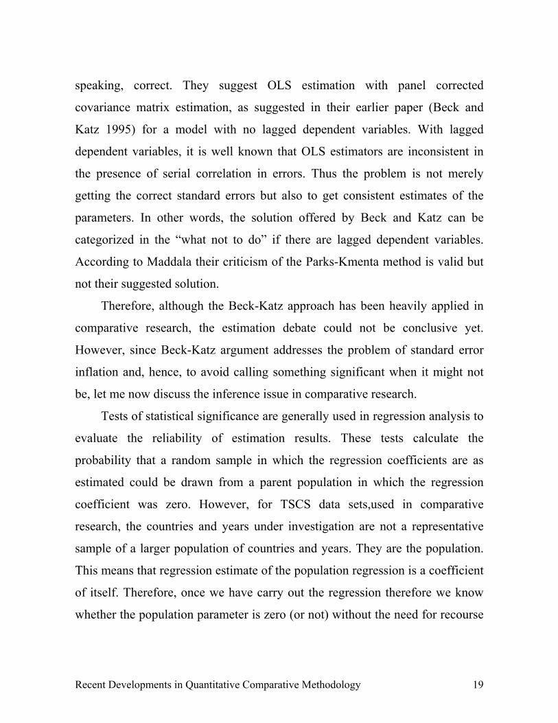
speaking, correct. They suggest OLS estimation with panel corrected

covariance matrix estimation, as suggested in their earlier paper (Beck and

Katz 1995) for a model with no lagged dependent variables. With lagged

dependent variables, it is well known that OLS estimators are inconsistent in

the presence of serial correlation in errors. Thus the problem is not merely

getting the correct standard errors but also to get consistent estimates of the

parameters. In other words, the solution offered by Beck and Katz can be

categorized in the “what not to do” if there are lagged dependent variables.

According to Maddala their criticism of the Parks-Kmenta method is valid but

not their suggested solution.

Therefore, although the Beck-Katz approach has been heavily applied in

comparative research, the estimation debate could not be conclusive yet.

However, since Beck-Katz argument addresses the problem of standard error

inflation and, hence, to avoid calling something significant when it might not

be, let me now discuss the inference issue in comparative research.

Tests of statistical significance are generally used in regression analysis to

evaluate the reliability of estimation results. These tests calculate the

probability that a random sample in which the regression coefficients are as

estimated could be drawn from a parent population in which the regression

coefficient was zero. However, for TSCS data sets,used in comparative

research, the countries and years under investigation are not a representative

sample of a larger population of countries and years. They are the population.

This means that regression estimate of the population regression is a coefficient

of itself. Therefore, once we have carry out the regression therefore we know

whether the population parameter is zero (or not) without the need for recourse


to probability theory (Comptson 1997, 741-2). Nevertheless, as Western and

Jackman (1994, 412-3) suggest, we can adopt a Bayesian approach of statistical

inference rather than the conventional statistical inference to address this

problem. In fact, the comparative researchers’ discomfort with frequentistic

inference is well founded because is not applicable to a no stochastic setting. It

is simply irrelevant for this problem to think of observations as drawn from a

random process when further realizations are impossible in practice, and lack

meaning even as abstract propositions. In contrast, the Bayesian model of the

statistical inference is a valid solution to this problem of the comparative

research. This is because the probability is conceived subjectively as

characterizing a researcher’s uncertainty about the parameters of statistical

model rather than a fact characterizing an object n the external world.

Consequently, for the Bayesian approach it is not relevant that data are not

generated by a repeatable mechanism such as coin flip.


3. Time and Space Effects

As we argued above, error complications can be also caused by model

misspecifications. If we assume that the level of the dependent variable is

homogeneous across time periods and units, we risk that error contains both

temporal and cross-section components reflecting, respectively, time effects

and cross-section effects. In particular, if different time periods and cross-

section are consistently higher or lower on the dependent variable, the common

intercept 1β estimated in OLS regression will be a average of all time period

and units that may not be representative for any one of the single groups of

observations.

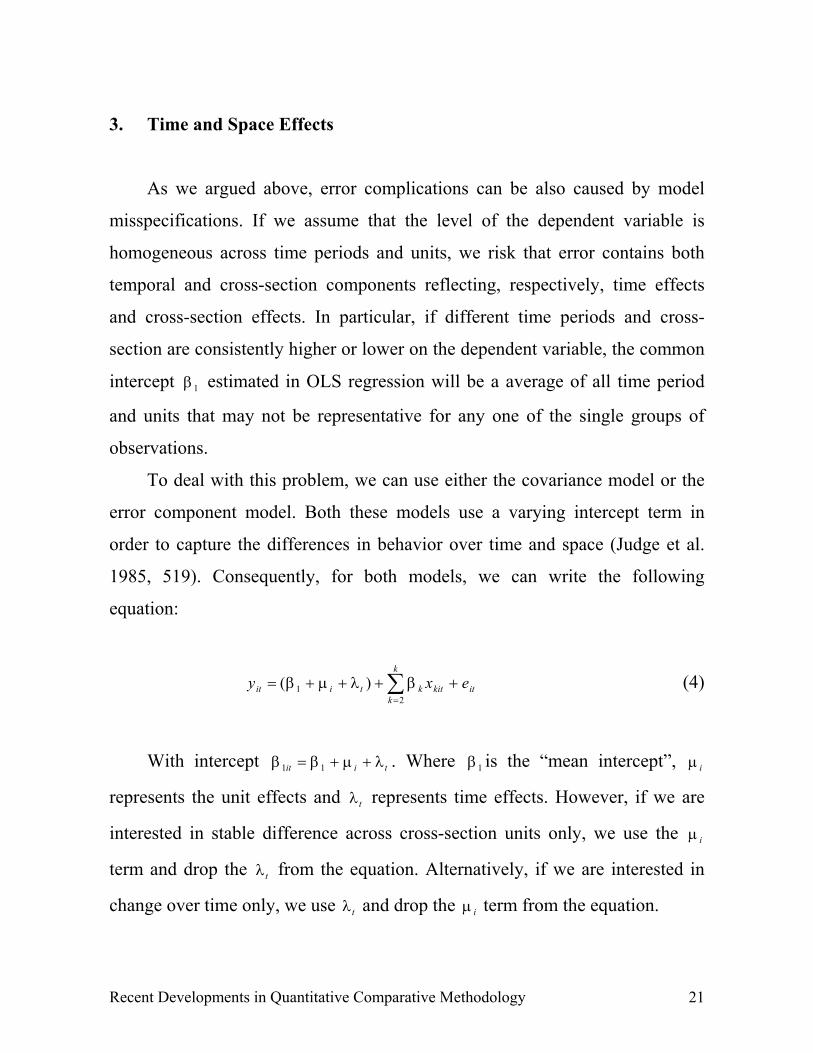
To deal with this problem, we can use either the covariance model or the

error component model. Both these models use a varying intercept term in

order to capture the differences in behavior over time and space (Judge et al.

1985, 519). Consequently, for both models, we can write the following

equation:

itkit

k

kktiit exy ++++= ∑

=21 )( βλµβ (4)

With intercept tiit λµββ ++= 11 . Where 1β is the “mean intercept”, iµ

represents the unit effects and tλ represents time effects. However, if we are

interested in stable difference across cross-section units only, we use the iµ

term and drop the tλ from the equation. Alternatively, if we are interested in

change over time only, we use tλ and drop the iµ term from the equation.


If the term iµ and tλ are fixed, the equation 4 is a covariance model (or a

dummy variable model). Conversely, when they are random, it is an error

component model. In other words, in the case of covariance model, the specific

characteristic of a cross-section units and of a time period are parameters; but,

using error component model the specific characteristic of a cross-section units

and of a time period are normally distributed random variables. Thus, in the

statistical literature, the error component model is kwon as a random effect

model, and the covariance model is referred to as a fixed effect model.

The reasoning underlying the covariance model is that in specifying the

regression model we have failed to include relevant explanatory variables that

do not change over time and/or others that do not change across cross-section

units, and hence the inclusion of dummy variables is a cover-up of our

ignorance (Kmenta 1986, 633). Conversely, the reasoning underlying the error

component model is that the relevant explanatory variables that we have

omitted random variables and, thus, iµ and/or tλ are drawn from a normal

distribution.

Regarding the covariance model as one with a varying intercept appears

reasonable because we address the unit and/or the period effects through the ad

hoc addition of dummy variables for cross-section units and/or time periods.

On the other hand, regarding error component model as one with a varying

intercept could appear arbitrary (Judge et al 1985, 522). In fact, it could also be

viewed as one where all coefficients are constant and the regression

disturbances are composed by three independent models (one component

associated with the time, one component associated with the space and the third

associated with both dimensions) (Kmenta 1986, 633). Consequently, for the


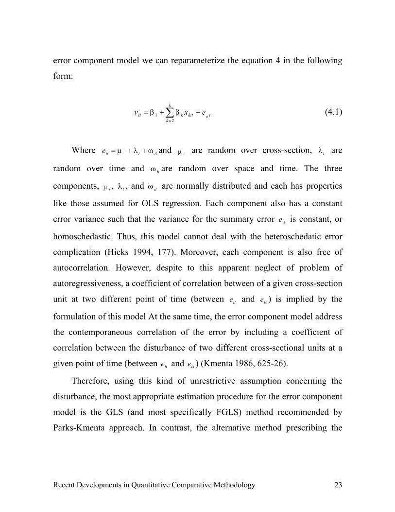
error component model we can reparameterize the equation 4 in the following

form:

tkit

k

kkit it

exy ++= ∑=2

1 ββ (4.1)

Where ittite ωλµ ++= and iµ are random over cross-section, tλ are

random over time and itω are random over space and time. The three

components, iµ , tλ , and itω are normally distributed and each has properties

like those assumed for OLS regression. Each component also has a constant

error variance such that the variance for the summary error ite is constant, or

homoschedastic. Thus, this model cannot deal with the heteroschedatic error

complication (Hicks 1994, 177). Moreover, each component is also free of

autocorrelation. However, despite to this apparent neglect of problem of

autoregressiveness, a coefficient of correlation between of a given cross-section

unit at two different point of time (between ite and ise ) is implied by the

formulation of this model At the same time, the error component model address

the contemporaneous correlation of the error by including a coefficient of

correlation between the disturbance of two different cross-sectional units at a

given point of time (between ite and ise ) (Kmenta 1986, 625-26).

Therefore, using this kind of unrestrictive assumption concerning the

disturbance, the most appropriate estimation procedure for the error component

model is the GLS (and most specifically FGLS) method recommended by

Parks-Kmenta approach. In contrast, the alternative method prescribing the


OLS with PCSEs is not especially appropriate for the error component model.

In fact, given that the error component model is heavily used in cross-sectional

dominant data set, Beck and Katz (1995, 645) do not consider this model. Their

proposal is limited to temporally dominant models.

Alternatively, for the covariance model, we can use either Beck-Katz

approach or Parks-Kmenta method. In this case the disturbance ite is supposed

to satisfy the assumption of the classical linear regression model. Moreover, as

Beck and Katz (1995, 645) note, this model presents no special problems,

especially when it is utilized in a temporally dominant model and it is allowed

intercepts to vary by unit only. This is because the number of unit-specific

dummy variables required is not large and, thus, the fixed effects do not use an

absurd number of degree of freedom.

However, we could allow ite to be autoregressive and heteroschedastic,

and then use the GLS (FGLS) estimation procedure for a covariance model

(Kmenta 1986, 630). In other words, the Parks-Kmenta method can be made to

address the unit and period effects through the ad hoc addition of dummy

variables for cross-section units, time periods, or both (Hicks 1994, 175).

Finally, let me briefly discuss the problem of the choice between these

models. Since assuming unit and/or time period effects to be fixed or random is

not obvious, the estimation procedure could not be chosen accordingly (Judge

et al.1985, 527). For example, consider a research where the dependent

variable, in additional to explanatory variables, is affected by a variable which

varies across units yet remains constant over time (as usually happens in

political economy research). Here, the inference concerning coefficients of

relevant explanatory variables could be unconditional with the respect to other


variables, or it could be conditional on the other variables. The advantage of

using the error component model is that we save a number of degree of

freedom and, then, obtain more efficient estimates of the regression parameters.

The disadvantage of using the error component model is that if the cross-

section characteristic is correlated with included explanatory variables, the

estimated regression coefficients are biased and inconsistent. The advantage of

the covariance model is that it protects us against a specification error caused

by such a correlation, but its disadvantage is a loss of efficiency due to the

increased number of parameters to be estimated. Therefore, the crucial

consideration is the possibility of a correlation between cross-sectional and/or

time period characteristics and included explanatory variables (Kmenta 1986,

634).

If there is doubt about the correlation between the cross-sectional characteristic

and the included explanatory variables, we may carry out a test of the null

hypothesis that not such correlation exists against the alternative hypothesis

that there is a correlation. For this purpose we can use the Hausman’s test.

Under the null hypothesis that 0)( =Ε iitx µ the GLS estimator of β of the

random effect model should not be very different from the least squares

estimator of β of the fixed effects model. Provided no other classical

assumption is violated, a statistically significant difference between these two

estimators indicates that )( iitx µΕ is different from zero (Kmenta 1986, 635).

This test is formally a test of equality of the coefficients estimated by the fixed

and the random effect estimator. If the coefficients differ significantly, either


the model is misspecified or the assumption that the random effect iµ are

correlated with the regressor itx is incorrect.

Nevertheless, since for several political economy models the fixed effects

cause serious econometric problems, the issue created becomes fixed effects vs.

no fixed effects, and not fixed effects vs. random effects. This is so because

these cases have many independent variables that change slowly over time, and

then the fixed effects are highly collinear with some of them. Consequently, in

many political economy researches, the analysts tend to not control for country

fixed effects (Beck 2000, 5). Nevertheless, Garrett and Mitchell (1999, 19)

consider this a mistake. This is because if a regressor varies only little over

time, but greatly across countries, and if the inclusion of country dummy has a

substantial effect on the direction, magnitude, or statistical significance of the

variable, the appropriate response is not to exclude the country dummies.

Rather, the analyst should conclude that the relevant variable is part the

underlying historical fabric of a country that affects the dependent variable and

that is not captured by any of the time and country-varying regressors. When

these fixed effects are taken into account, the apparent effect of year-to-year

fluctuations in the variable could well be very different than when country

dummies are not included.


4. Pooling Dilemma and Causal Heterogeneity

These models do not address the problem 5. They do not consider that the

error tends to be nonrandom across spatial and/or temporal units because

parameters (like the underlying processes that they reflect) are heterogeneous

across subsets of units. In fact, for the fixed effect model, the random effect

model and the simpler pooled model, the slope coefficients are assumed to be

equal over time and space. The homogeneity of slope coefficients is often an

unreasonable assumption (Maddala et al. 1997, 90).

The solution frequently suggested is to apply a preliminary test of

significance to test the equality of the coefficients and decide not to pool if this

hypothesis is rejected and to pool if this hypothesis is not rejected.

Consequently, the question becomes: to pool or not to pool? The question is

whether to estimate the models separately for different cross-section units or

for different time series, or to estimate the model by pooling the entire data set

and, thus, by estimating a model with coefficients that are constant across units

and time periods (Maddala 1991, 302).

Kittel’s proposal concerns these two extreme cases of complete

homogeneity and complete heterogeneity. He (1999, 232-43) argues that the

constant coefficient model in TSCS analysis (without any inclusion of fixed or

random effects) represents the combined average partial effect for both time

and space. It does not yield information about the relative contribution of two

dimensions to its value. In other words, without additional analysis the question

of the whether cross-country differences or cross-specific developments

account for the variation goes unanswered. Consequently, to inspect the


development of the relation over time, we estimate repeated cross-section

regression analysis. In particular, by estimating yearly cross-sectional models,

we can evaluate whether the relationship between the dependent variable and

independent variables changes over the period investigated or whether it

remains constant as the constant coefficient model prescribes. A second method

of validating pooled coefficients compares the time series of the countries

analyzed. Since in the comparative political economy research several

explanatory variables tend to vary across countries, but are constant or change

within many countries, we cannot assess the relationship of the time series

dimensions. However, this indicates as a further restriction to the sensitive use

of the constant coefficient approach to the pooling. Being based on mostly

constant data in the time series dimension, the pooled coefficients of these

variables rely almost completely on the cross-section dimension.

Therefore, according to Kittel (1999, 232-3), these problems do not mean

that pooling is not worth the effort. They simply point to the proviso that the

data set should be analyzed with care and that reporting pooling coefficients in

the pooling constant coefficients model without further evaluation of the

relative contributions of the space and time dimensions to the coefficients can

lead to unwarranted conclusions.

However, between these two extreme cases of the complete homogeneity

of the constant coefficient model and of the complete heterogeneity of the

separate estimation of cross-section or time series coefficients, there are more

appropriate intermediate solutions. The problem with these two estimation

methods of either pooling the data or obtaining separate estimates for each

cross-section or time series is that both are based on extreme assumptions. The


parameters are assumed to be all the same or all different in the each cross-

section and/or time series. The truth probably lies somewhere in between.. The

parameters are not exactly the same, but there is some similarity between them

(Maddala et al. 1997, 91). One way of allowing for the similarity is to assume

that the parameters all vary over time or/and units. However, in this paper I will

concentrate only on the cross-section heterogeneity. This is because, although

they are not significantly applied in the comparative research yet, they

represent critical methodological issues regarding the pooled analysis. From a

substantive perspective, a key idea of comparative research is that causal

process varies across countries. The fundamental problem in the comparative

research contextual explanation where the differences in the causal processes

within countries are related to characteristics that varies across countries. This

contextual idea is expectably relevant to the comparative political economy. In

this area cross-national variation in economic relationships originated with

enduring institutional differences (Western 1998, 1255). Therefore, with causal

heterogeneity depending on cross-national variation in the institutions, model

with slope coefficients that vary over cross-sectional units provide a closer fit

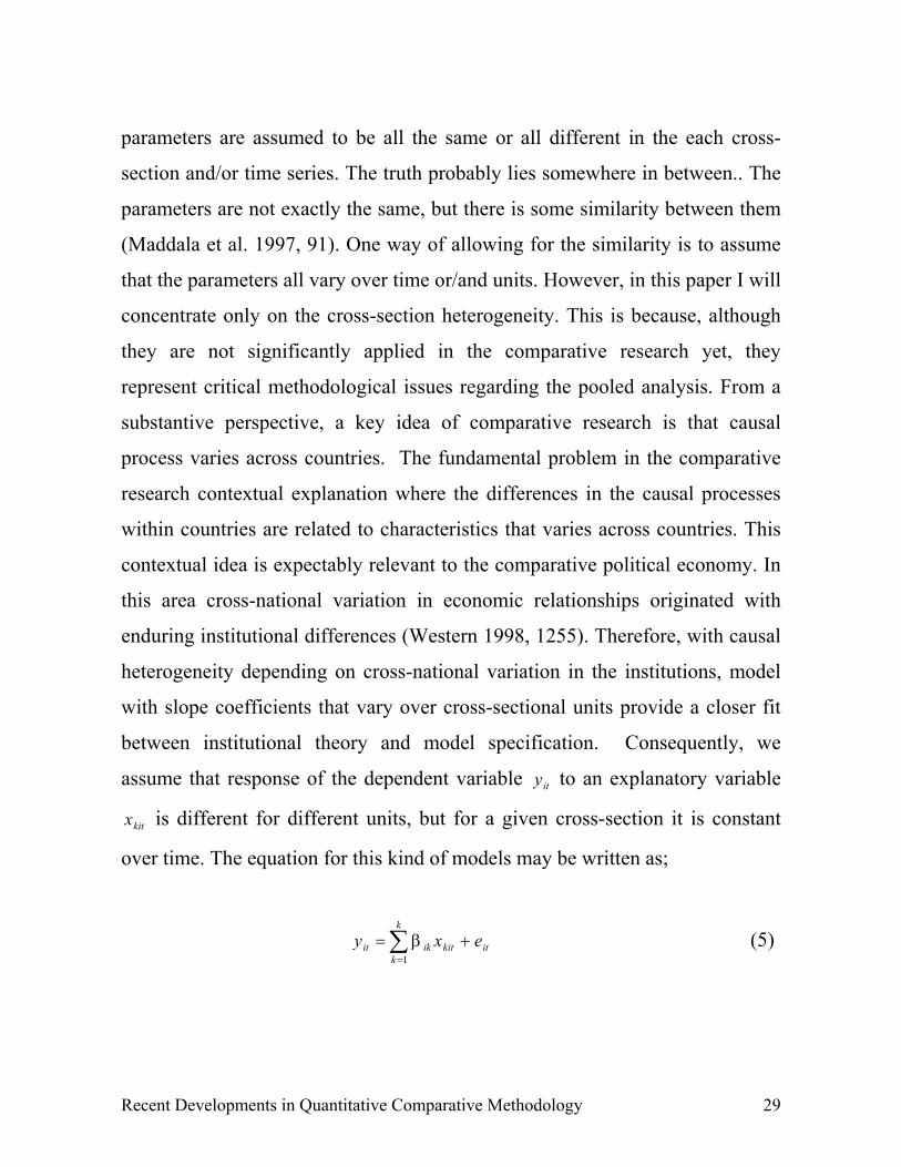
between institutional theory and model specification. Consequently, we

assume that response of the dependent variable ity to an explanatory variable

kitx is different for different units, but for a given cross-section it is constant

over time. The equation for this kind of models may be written as;

itkit

k

kikit exy +=∑

=1β (5)


itkit

k

kki ex ++=∑

=

)(1

αβ

In contrast to previous equations I no longer treat the constant term

differently from the other explanatory variables. ).....( 1 kβββ = can be viewed as

the common-mean coefficient vector and ).....( 1 kiii ααα = as the individual

deviation from the common mean. When kiβ are treated as fixed and different

constants, equation 5 can be viewed as the seemingly unrelated regression

model. Conversely, when kiβ are treated as random parameters, equation 5 is

equivalent to the random coefficient model (Judge et al. 1985, 538-9; Hsiao

1986, 130-1).

The seemingly unrelated regression model treats each cross-section and

the time series within that cross-section as a separate equation that is unrelated

to any other cross-section (and time series within the cross-section) in the

pooled data set. Most specifically, this model is interpretable as a series of a

nation specific regression analysis that utilizes contemporaneous cross-equation

error correlations among the error of a system of equation to improve the

efficiency of the equation’s estimates (Sayrs 1989, 39; Hicks 1994, 181).

The random coefficient model is due to Swamy (1970). This model

assumes that each iβ are drawn from a common normal distribution In other

words, ii αββ += are treated as random, with a common mean. The model set

up is:

);(~ ^Ii ββ (5.1)


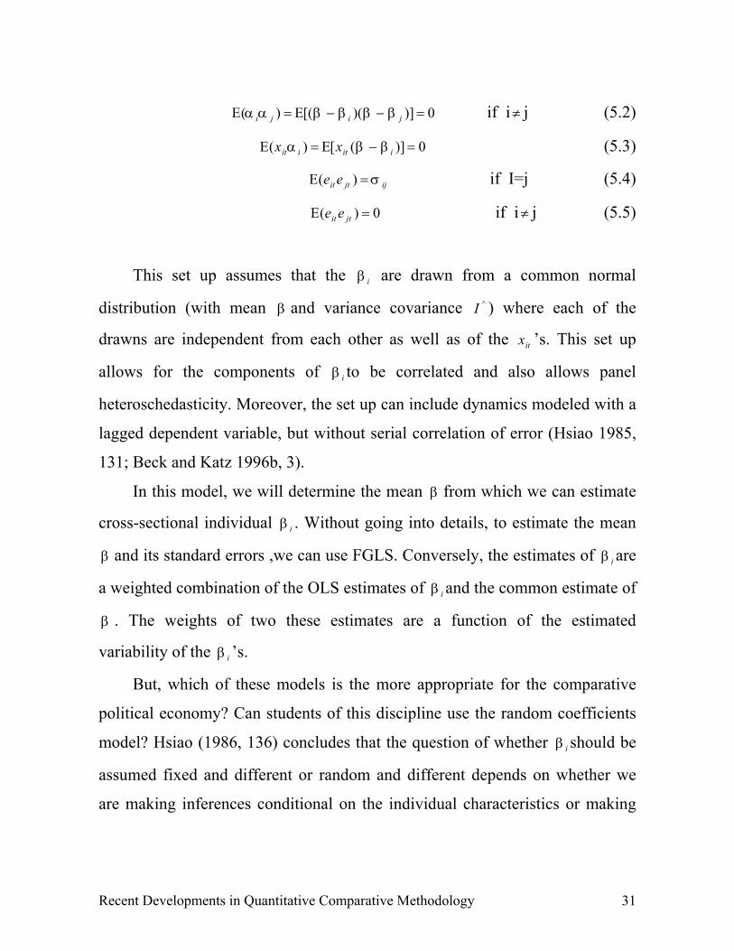
0)])([()( =−−Ε=Ε jiji ββββαα if i≠ j (5.2)

0)]([)( =−Ε=Ε iitiit xx ββα (5.3)

ijjtit ee σ=Ε )( if I=j (5.4)

0)( =Ε jtit ee if i≠ j (5.5)

This set up assumes that the iβ are drawn from a common normal

distribution (with mean β and variance covariance ^I ) where each of the

drawns are independent from each other as well as of the itx ’s. This set up

allows for the components of iβ to be correlated and also allows panel

heteroschedasticity. Moreover, the set up can include dynamics modeled with a

lagged dependent variable, but without serial correlation of error (Hsiao 1985,

131; Beck and Katz 1996b, 3).

In this model, we will determine the mean β from which we can estimate

cross-sectional individual iβ . Without going into details, to estimate the mean

β and its standard errors ,we can use FGLS. Conversely, the estimates of iβ are

a weighted combination of the OLS estimates of iβ and the common estimate of

β . The weights of two these estimates are a function of the estimated

variability of the iβ ’s.

But, which of these models is the more appropriate for the comparative

political economy? Can students of this discipline use the random coefficients

model? Hsiao (1986, 136) concludes that the question of whether iβ should be

assumed fixed and different or random and different depends on whether we

are making inferences conditional on the individual characteristics or making


unconditional inferences on the population characteristics. In the former cases,

fixed-coefficients model should be used. In the latter cases, the random

coefficients model should be used.

Such a conclusion indicates that the random coefficients model is

appropriate for panel studies in survey research rather than for comparative

TSCS analysis. This is because in the panel data the observed “people” are of

no interest per se, with all of inferences of interest being to the underlying

population that was sampled. TSCS data show the opposite situation. Here, all

inferences of interest are conditional on the observed units (Beck 2000, 3)

However, one way to avoid this problem is to use Bayesian approach. As

Beck and Katz (1996, 5) suggest, the advantage of Bayesian linear hierarchical

model is that the randomness resides in the parameters, and not the units.

Hence, the distinction between fixed and sampled units is no longer relevant.

This approach yields identical results to the random coefficients model. Here,

we have a prior on the variability of the iβ ’s, which looks like equation 5.1.

This assumes that iβ are “exchangeable”, since a priori we cannot distinguish

between the units other than through the covariates. The Bayesian approach lets

the data choose the prior using the estimated structure of ^I as the prior of

parameter variability. However, from the Bayesian perspective letting the data

choose the prior appears a bit odd. Bayesians have prior beliefs about the

diversity of iβ . Thus, these priors can be combined with the observed data (via

likelihood function) to produce a new, posterior, set of beliefs about the iβ .

The prior which is represented by ^I , is based on the analyst’s belief about the


world rather than a parameter to be estimated. The prior ^I than can be

combined with the OLS estimates of iβ .

However, the Bayesian hierarchical model can be made more useful for

comparative research by allowing the iβ to be a function of the other unit

variables, which allow modeling differential effects as a function of different

institutions. In fact, as Western (1998, 1241) notes, in the Beck and Katz’s

(1996b) model institutional effect and the issue of contextual explanation are

omitted. Consequently, one can allow the iβ to be function of other unit

variable, iz , which allows for modeling effects as a function of differing

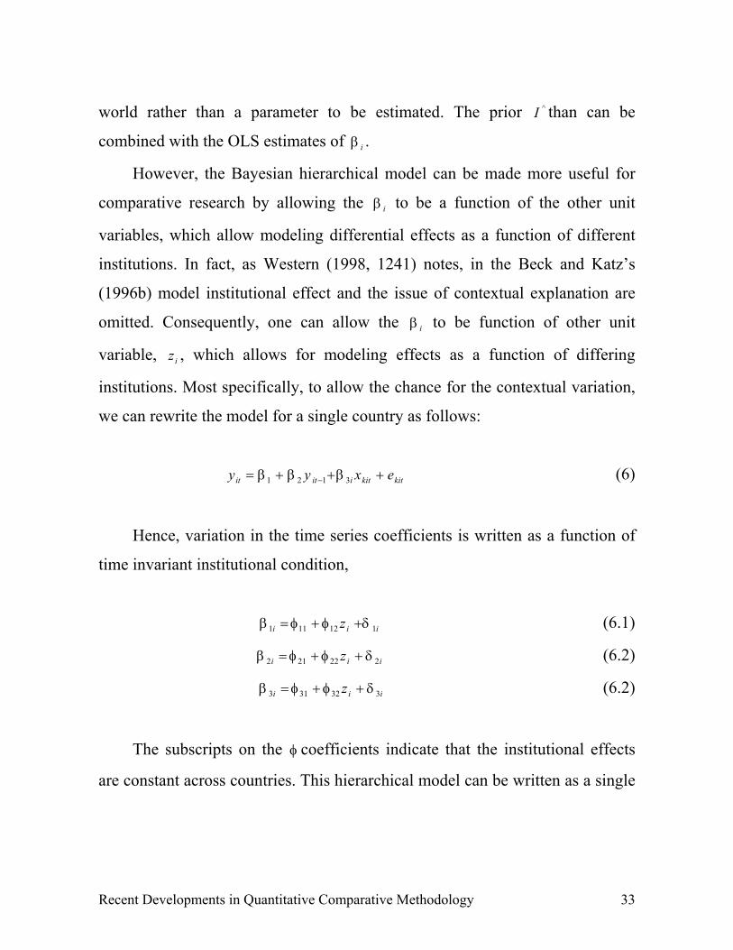
institutions. Most specifically, to allow the chance for the contextual variation,

we can rewrite the model for a single country as follows:

kitkitiitit exyy +++= − 3121 βββ (6)

Hence, variation in the time series coefficients is written as a function of

time invariant institutional condition,

iii z 112111 δφφβ ++= (6.1)

iii z 222212 δφφβ ++= (6.2)

iii z 332313 δφφβ ++= (6.2)

The subscripts on the φ coefficients indicate that the institutional effects

are constant across countries. This hierarchical model can be written as a single


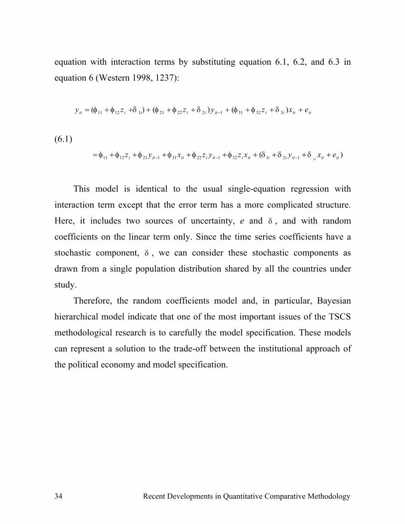
equation with interaction terms by substituting equation 6.1, 6.2, and 6.3 in

equation 6 (Western 1998, 1237):

ititiiitiiiiit exzyzzy +++++++++= − )()()( 3323112222111211 δφφδφφδφφ

(6.1)

)(312132122311211211 itititiiitiitiititi exyxzyzxyz

i+++++++++= −−− δδδφφφφφφ

This model is identical to the usual single-equation regression with

interaction term except that the error term has a more complicated structure.

Here, it includes two sources of uncertainty, e and δ , and with random

coefficients on the linear term only. Since the time series coefficients have a

stochastic component, δ , we can consider these stochastic components as

drawn from a single population distribution shared by all the countries under

study.

Therefore, the random coefficients model and, in particular, Bayesian

hierarchical model indicate that one of the most important issues of the TSCS

methodological research is to carefully the model specification. These models

can represent a solution to the trade-off between the institutional approach of

the political economy and model specification.


5. Pooled TSCS analysis in STATA software

Finally, this section presents some implementations and commands in

STATA software to analyze TSCS data. Several econometric packages for

pooled models are now widely available (SAS and SHAZAM). However, I will

consider STATA only, assuming that the reader is familiar with the basics of

this statistical software.

The “xt” series of STATA commands provide tools for analyzing cross-

sectional time series data sets. Cross-sectional time series (longitudinal) data

sets are of form itx , where itx is a vector of observations for unit i and time t.

The particular commands as such “xtreg”, “xtgls” and “xtpcse” allow us to

estimate the majority of pooled models discussed in this paper. Since TSCS

data sets are characterized by both unit i and time t dimensions, corresponding

STATA options are usually required to estimate pooled models using these

commands. The option “i( )” sets the name of the variable corresponding to the

unit. The option “t( )” sets the name of the variable corresponding to the time

index t (STATA 1999, 317). Given that in the comparative analysis these

variables are often represented by “country” and “year”, in the next examples I

will use these variable names. Moreover, for expository purpose, let me

suppose that we have data of the following form: y (dependent variable), and

x1, x2, x3 (respectively, 1st predictor, 2nd predictor and 3rd predictor).

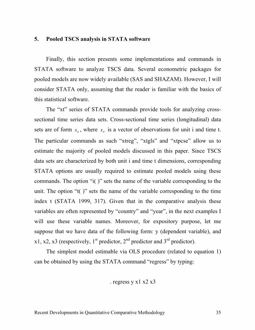
The simplest model estimable via OLS procedure (related to equation 1)

can be obtained by using the STATA command “regress” by typing:

. regress y x1 x2 x3


Hover, as noted, TSCS designs often violate the standard OLS

assumptions, first we need to consider STATA implementations concerning

Parks-Kmenta method and Beck-Katz approach. Regarding the Parks-Kmenta

approach, the “xtgls” command estimates models using FGLS procedure. This

command allows estimation in presence of AR(1) autocorrelation within units,

cross-sectional correlation and/or heteroschedasticity across units. In other

words, the model related to the equation 2 can be estimated by “xtgls” STATA

command and the assumptions concerning the panel heteroschedasticity,

contemporaneous correlation and serial correlation can be obtained by

specifying particular options (STATA 1999, 360-69). The heteroschedastic

models obtained by specifying by:

. xtgls y x1 x2 x3, i(country) panels(heteroschedastic)

However, we may wish to assume that the error terms are correlated in

additional to having different variances. Hence, we must specify:

. xtgls y x1 x2 x3, i(country) t(year) panels(correlated)

Finally, “xtgls” allows different options so that you may assume serial

correlation within units. If we assume a serial correlation where the correlation

parameter is common for all units, we must specify the following command:

. xtgls y x1 x2 x3, i(country) t(year) corr(ar1)


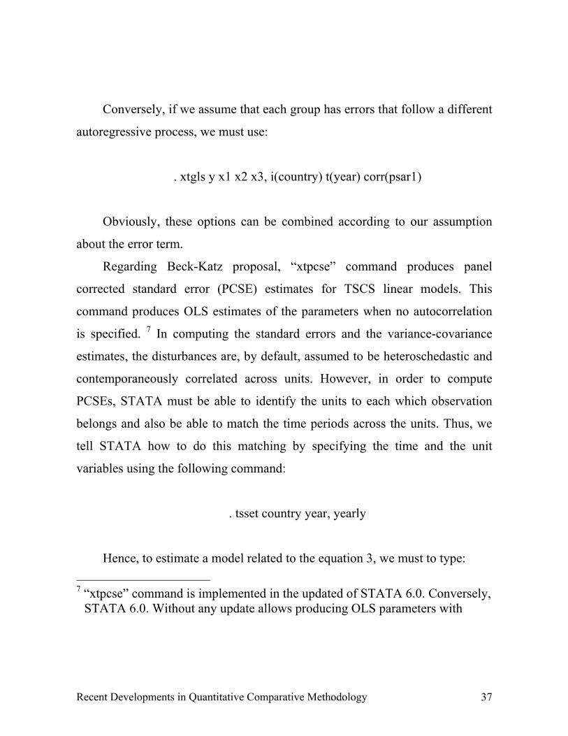
Conversely, if we assume that each group has errors that follow a different

autoregressive process, we must use:

. xtgls y x1 x2 x3, i(country) t(year) corr(psar1)

Obviously, these options can be combined according to our assumption

about the error term.

Regarding Beck-Katz proposal, “xtpcse” command produces panel

corrected standard error (PCSE) estimates for TSCS linear models. This

command produces OLS estimates of the parameters when no autocorrelation

is specified. 7 In computing the standard errors and the variance-covariance

estimates, the disturbances are, by default, assumed to be heteroschedastic and

contemporaneously correlated across units. However, in order to compute

PCSEs, STATA must be able to identify the units to each which observation

belongs and also be able to match the time periods across the units. Thus, we

tell STATA how to do this matching by specifying the time and the unit

variables using the following command:

. tsset country year, yearly

Hence, to estimate a model related to the equation 3, we must to type: 7 “xtpcse” command is implemented in the updated of STATA 6.0. Conversely,

STATA 6.0. Without any update allows producing OLS parameters with


. xtpcse y ly x1 x2 x3

Where ly stands for a lagged dependent variable of one year. It can be

obtained by typing:

. generate ly = y[_n-1]

Let me now consider fixed and random effect models. For both these

models we can refer to the equation 4 when includes the unit effect term and

drops the time effect term. In fact, STATA considers the case in which fixed

and random effect model include the unit effects only. The command to

estimate this models is “xtreg” (STATA 1999, 420-40). In particular, to obtain

an OLS fixed effect model, we must to type:

. xtreg y x1 x2 x3, fe

Conversely, to obtain a GLS random effect model, we must type:

. xtreg y x1 x2 x3, re

After “xtreg, re” estimation we can obtain the Hausman test by typing:

. xthaus

PCSES by specifying “xtgls” with the “ols” or “pcse” option (STATA 1999,364).


However, the dummy variables are not included in the outputs

corresponding to these STATA commands. But, since fixed effect regression is

supposed to produce the same coefficient estimates as standard error as

ordinary regression when dummy variables are included for each units, to

obtain an output including dummy variables we must type:

. xi: regress y x1 x2 x3 i.country

Where “xi” command allows us to create dummy variables. Consequently,

by using this command with either “xtgls” or “xtpcse” respectively Parks-

Kmenta method or Beck-Katz approach can be made to address unit effects.

Let me now consider the models with slope coefficients that vary across

units, represented by equation 5. The STATA command to estimate a

seemingly unrelated regression model is “sureg”. However, in order to estimate

a simultaneous equation model using “sureg”, we should first reshape our data

(STATA 1999, 415). In other words, we need to convert our data from “long to

“wide” form by typing:

. reshape y x1 x2 x3, i(year) j(country)

Hence, we can estimate a seemingly unrelated regression model by typing:

. sureg (y1 x11 x21 x31) (y2 x12 x22 x32) (y3 x13 x23 x33)


Where the numbers 1, 2, 3 associated to the variables y x1 x2 x3 represent

the different countries of an example with three cases only.

Conversely, to estimate a random coefficient model, we do not need to

reshape our cross-sectional time series data set. To obtain such a model it is

enough typing the following command:

.xtrchh y x1 x2 x3, i(country) t(year)

STATA uses FGLS procedure to estimate random coefficients models, as

suggested by Swamy (1971), assuming that all coefficients are drawn from a

common multivariate normal distribution.8 The requirement of the random

coefficients model that that all variables) with random coefficients) vary within

units, may cause difficulty for comparative politics applications. where it is

frequently the case that some important variables are time invariant national

characteristics (Beck and Katz 1996b, 9). Nevertheless, STATA does not allow

assuming that the coefficients of some variables are fixed.9

Finally, regarding hierarchical models, software is now available (Western

1998, 1244). An extensive review of five packages for hierarchical modeling is

reported by Kreft et al. ( 1994). In additional to specialized software, routine

can also be found in the general statistical software SAS and S-PLUS (see

Pinheiro and Douglas 2000).

8 Such a procedure can cause some problems to estimate the variance matrix of

the error. For full details see Beck (2000, 19-20).9 Conversely, LIMPDEP 7.0. allows the investigator to specify whether

variables have fixed or random coefficients (see Greene 1995).


Bibliography:

Alesina A., Grilli V. and Milesi-Ferretti G. M., 1994, The Political Economy of Capital Controls, in L. Leiderman and A. Razin,(edited by), Capital Mobility, Cambridge, Cambridge University Press.

Alvarez M., Garrett G., and Lange P., 1991, Government Partnership, Labour Organization and MacroeconomicPerformance: 1967-1984, in American Political Journal Review, 85, pp. 539-556.

Beck N., 2000,Issues in the Analysis of Time-Series Cross-Section Data in the Year 2000,University of California, Manuscript.

Beck N. and. Katz J.N, 1995, What To Do (and Not To Do) with Time-Series Cross-Section Data, inAmerican Political Journal Review, 89, pp. 634-647.

Beck, N. and Katz J.N, 1996, Nuisance vs. Substance: Specifying and Estimating Time-Series-Cross-SectionModels, Political Analysis, 6, 1-36.

Beck, N. and Katz J.N., 1996b, Lumpers and Splitters United: The Random Coefficients Model, Presented atthe annual meeting of the Methodology Political Group, Ann Arbor, Michigan.

Beck, N. and Katz J.N., 1998, Taking Time Seriously: Time-Series-Cross-Section Analysis with a BinaryDependent Variable, in American Journal of Political Sciences, 42(4), pp.1260-1288.

Beck, N, Katz J.N., Alvarez M., Garrett G., and Lange P., 1993, Government Partisanship, Labor Organization, and MacroeconomicPerformance: A Corrigendum, American Political Journal Review, 67(4). pp.945-948


Compston H., 1997, Union Power, Policy-Making and Unemployment in Western Europe:1972-1993, in Comparative Political Studies, 30(6), pp. 732-751

Garrett, G., 1998, Partisan Politics in the Global Economy, Cambridge, Cambridge UniversityPress.

Garrett, G. and Mitchell D., 1999, Globalization and the Welfare State, Yale University, Manuscript.

Hicks A., 1991, Union, Social Democracy, Welfare and Growth, Research in PoliticalSociology, 5, pp. 209-234

Hicks A., 1994, Introduction to Pooling, in T. Janoski and A. Hicks (edited by), TheComparative Political Economy of the Welfare State, Cambridge UniversityPress

Hsiao C., 1986,Analysis of Panel Data, Cambridge University Press

Huber E., Ragin C., and Stephens J.D., 1993, Social Democracy, Christian Democracy, Constitutional Structure, and theWelfare State, American Journal of Sociology, 99(3) pp. 711-749

Judge G.G., Griffiths W.E., Hill R.C., Lutkepohl H. and Lee T-C., 1985, The Theory and Practice of Econometrics, New York, Wiley, 2nd Ed

Kittel B., 1999,Sense and Sensitivity in Pooled Analysis in Political Data, in European Journalof Political Research, 35(2), pp. 225-253

Kmenta, J., 1986,


Elements of Econometrics. New York: Macmillan; London: Collier Macmillan,2nd Ed.

Maddala, G.S., 1994, To Pool or Not to Pool: That is the Question, in Maddala G.S. ,(edited by),Econometric Method and Applications, Edward Elgart

Maddala, G.S., 1997, Recent Developments in Dynamics Econometric Modeling: A PersonalViewpoint, Ohio State University, Manuscript.

Maddala, G.S., H. Li, R.P. Trost and F. Joutz (1997), 'Estimation of Short-Run and Long-Run Elasticities of Energy Demand FromPanel Data Using Shrinkage Estimators, Journal of Business Economics andStatistics, 15, pp. 90-100

Oatley T., 1993, How Constraining is Capital Mobility? The Partisan Hypothesis in an OpenEconomy, in American Journal of Political Sciences, 43(4) pp. 1003-1027

Pampel F.C. and Williamson G.B., 1989, Age, Class, Politics and the Welfare State, Cambridge, Cambridge UniversityPress

Parks R.W., 1966, Efficient Estimation of a System of Regression Equation When Disturbance areBoth Serially and Contemporaneously Correlated, in Journal of the AmericanStatistical Association, 62, 500-509

Pennings P., Keman H. and Kleinnijenhuis: J., 1999, Doing Research in Political Science: An Introduction to Comparative Methodsand Statistics, Sage,

Quinn, D. P. and Inclan, C., 1997, The Origins of Financial Openness, in American Journal of Political Sciences,41(3), pp. 771-813


Sayrs, L.W., 1989, Pooled Time Series Analysis, Sage Publications

Schmidt M.G., 1997, Determinants of Social Expenditure in Liberal Democracies, in Acta Politica,32(2) pp. 153-173

Stimson, J.A., 1985, Regression in Space and Time: A Statistical Essay, in American Journal ofPolitical Sciences, 29(4) pp. 914-947

Swamy P.A.P.V. 1970, Efficient Inference in a Random Coefficients Regression Model, Econometrica,32, pp. 313-323

Swank D.H., 1992, Structural Power and Capital Investment in the Capitalists Democracies, inAmerican Political Journal Review, 86, pp. 38-54

Western, B., 1998, Causal Heterogeneity in Comparative Research: A Bayesian HierarchicalModeling Approach, in American Journal of Political Sciences, 42(4), pp.1233-1259.

Western B. and Jackman S., 1994, Bayesian Inference for Comparative Research, American Political JournalReview, 88(2), pp. 412-423

pooled time series

Documents